.

1 Mathematical ModelsA Catalog of Essential Functions

11.2.2

22

Mathematical Models: A Catalog of Essential Functions

A mathematical model is a mathematical description (often by means of a function or an equation) of a real-world phenomenon such as the size of a population, the demand for a product, the speed of a falling object, the concentration of a product in a chemical reaction, the life expectancy of a person at birth, or the cost of emission reductions.

The purpose of the model is to understand the phenomenon and perhaps to make predictions about future behavior.

33

Mathematical Models: A Catalog of Essential Functions

Figure 1 illustrates the process of mathematical modeling.

Figure 1

The modeling process

44

Mathematical Models: A Catalog of Essential Functions

A mathematical model is never a completely accurate representation of a physical situation—it is an idealization. A good model simplifies reality enough to permit mathematical calculations but is accurate enough to provide valuable conclusions.

It is important to realize the limitations of the model. In the end, Mother Nature has the final say.

There are many different types of functions that can be used to model relationships observed in the real world. In what follows, we discuss the behavior and graphs of these functions and give examples of situations appropriately modeled by such functions.

55

Linear Models

66

Linear Models

When we say that y is a linear function of x, we mean that the graph of the function is a line, so we can use the slope-intercept form of the equation of a line to write a formula for the function as

y = f (x) = mx + b

where m is the slope of the line and b is the y-intercept.

77

Linear Models

A characteristic feature of linear functions is that they grow at a constant rate.

For instance, Figure 2 shows a graph of the linear function f (x) = 3x – 2 and a table of sample values.

Figure 2

88

Linear Models

Notice that whenever x increases by 0.1, the value of f (x) increases by 0.3.

So f (x) increases three times as fast as x. Thus the slope of the graph y = 3x – 2, namely 3, can be interpreted as the rate of change of y with respect to x.

99

Example 1

(a) As dry air moves upward, it expands and cools. If the ground temperature is 20C and the temperature at a height of 1 km is 10C, express the temperature T (in °C) as a function of the height h (in kilometers), assuming that a linear model is appropriate.

(b) Draw the graph of the function in part (a). What does the slope represent?

(c) What is the temperature at a height of 2.5 km?

1010

Example 1(a) – Solution

Because we are assuming that T is a linear function of h, we can write

T = mh + b

We are given that T = 20 when h = 0, so

20 = m • 0 + b = b

In other words, the y-intercept is b = 20.

We are also given that T = 10 when h = 1, so

10 = m • 1 + 20

The slope of the line is therefore m = 10 – 20 = –10 and the required linear function is

T = –10h + 20

1111

Example 1(b) – Solution

The graph is sketched in Figure 3.

The slope is m = –10C/km, and this represents the rate of change of temperature with respect to height.

Figure 3

cont’d

1212

Example 1(c) – Solution

At a height of h = 2.5 km, the temperature is

T = –10(2.5) + 20 = –5C

cont’d

1313

Linear Models

If there is no physical law or principle to help us formulate a model, we construct an empirical model, which is based entirely on collected data. We seek a curve that “fits” the data in the sense that it captures the basic trend of the data points.

1414

Polynomials

1515

Polynomials

A function P is called a polynomial if

P (x) = anxn + an–1xn–1 + . . . + a2x2 + a1x + a0

where n is a nonnegative integer and the numbers a0, a1, a2, . . ., an are constants called the coefficients of the polynomial.

The domain of any polynomial is If the leading coefficient an 0, then the degree of the polynomial is n. For example, the function

is a polynomial of degree 6.

1616

Polynomials

A polynomial of degree 1 is of the form P (x) = mx + b and so it is a linear function.

A polynomial of degree 2 is of the form P (x) = ax2 + bx + c and is called a quadratic function.

1717

Polynomials

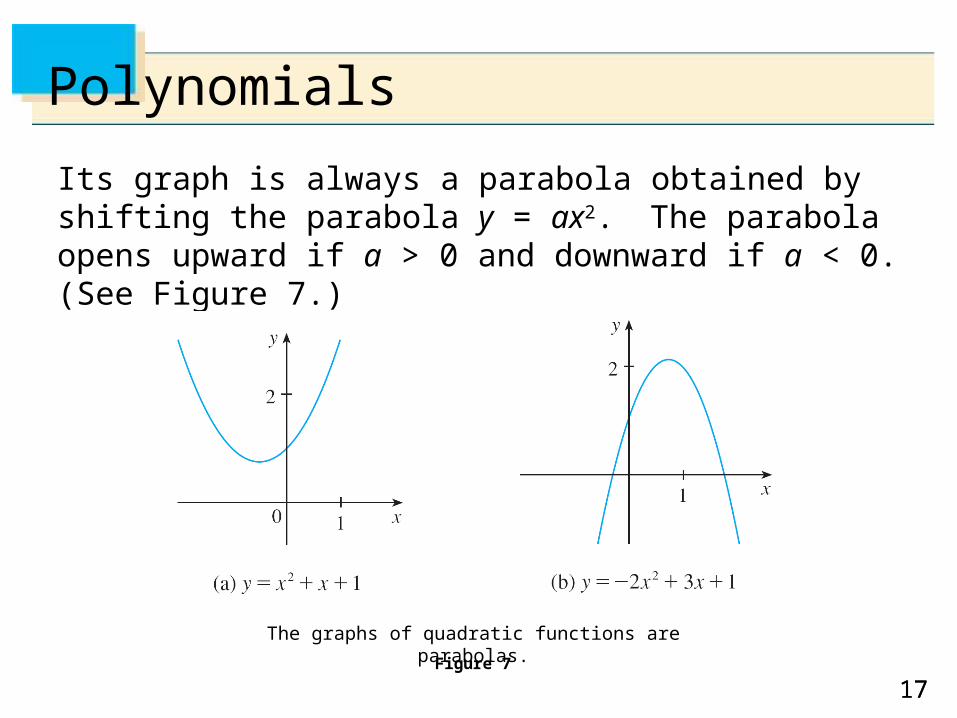
Its graph is always a parabola obtained by shifting the parabola y = ax2. The parabola opens upward if a > 0 and downward if a < 0. (See Figure 7.)

Figure 7

The graphs of quadratic functions are parabolas.

1818

Polynomials

A polynomial of degree 3 is of the form

P (x) = ax3 + bx2 + cx + d a 0

and is called a cubic function. Figure 8 shows the graph of a cubic function in part (a) and graphs of polynomials of degrees 4 and 5 in parts (b) and (c).

Figure 8

1919

Power Functions

2020

Power Functions

A function of the form f(x) = xa, where a is a constant, is called a power function. We consider several cases.

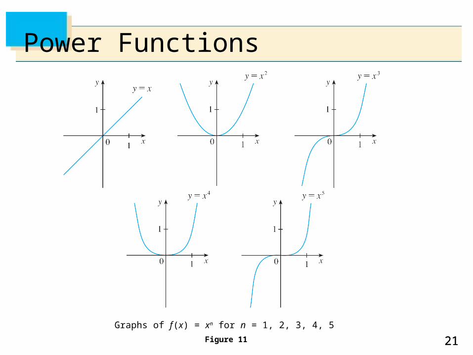
(i) a = n, where n is a positive integerThe graphs of f(x) = xn for n = 1, 2, 3, 4, and 5 are shown in Figure 11. (These are polynomials with only one term.)

We already know the shape of the graphs of y = x (a line through the origin with slope 1) and y = x2 (a parabola).

2121

Power Functions

Graphs of f (x) = xn for n = 1, 2, 3, 4, 5

Figure 11

2222

Power Functions

The general shape of the graph of f (x) = xn depends on whether n is even or odd.

If n is even, then f (x) = xn is an even function and its graph is similar to the parabola y = x2.

If n is odd, then f (x) = xn is an odd function and its graph is similar to that of y = x3.

2323

Power Functions

Notice from Figure 12, however, that as n increases, the graph of y = xn becomes flatter near 0 and steeper when | x | 1. (If x is small, then x2 is smaller, x3 is even smaller,x4 is smaller still, and so on.)

Families of power functions

Figure 12

2424

Power Functions

(ii) a = 1/n, where n is a positive integer

The function is a root function. For n = 2 it is the square root function whose domain is [0, ) and whose graph is the upper half of theparabola x = y2. [See Figure 13(a).]

Figure 13(a)

Graph of root function

2525

Power Functions

For other even values of n, the graph of is similar to that of

For n = 3 we have the cube root function whose domain is (recall that every real number has a cube root) and whose graph is shown in Figure 13(b). The graph of for n odd (n > 3) is similar to that of

Graph of root function

Figure 13(b)

2626

Power Functions

(iii) a = –1The graph of the reciprocal function f (x) = x

–1 = 1/x is shown in Figure 14. Its graph has the equation y = 1/x, or xy = 1, and is a hyperbola with the coordinate axes as itsasymptotes.

The reciprocal function

Figure 14

2727

Power Functions

This function arises in physics and chemistry in connection with Boyle’s Law, which says that, when the temperature is constant, the volume V of a gas is inversely proportional to the pressure P:

where C is a constant.

Thus the graph of V as a function of P (see Figure 15) has the same general shape as the right half of Figure 14.

Figure 15

Volume as a function of pressureat constant temperature