© 2012 daniel a. koch - university of...
TRANSCRIPT

1
COMPARISON OF REINFORCED CONCRETE BEAMS AND COR-TUF BEAMS UNDER IMPACT LOADING
By
DANIEL A. KOCH
A THESIS PRESENTED TO THE GRADUATE SCHOOL OF THE UNIVERSITY OF FLORIDA IN PARTIAL FULFILLMENT
OF THE REQUIREMENTS FOR THE DEGREE OF MASTER OF ENGINEERING
UNIVERSITY OF FLORIDA
2012

2
© 2012 DANIEL A. KOCH

3
To my loving and supportive family and my always supportive girlfriend

4
ACKNOWLEDGMENTS
First and foremost, I want to thank my thesis advisor, Dr. Theodor Krauthammer,
for all of his invaluable assistance and guidance. I would also like to thank my thesis
committee member, Dr. Serdar Astarlioglu for all of his help with the Dynamic Structural
Analysis Suite (DSAS) software and writing critiques. Additionally, I want to thank Dr.
Long Hoang Bui for his assistance with the finite element software and material models.
Furthermore, I would like to acknowledge the sponsors of my work, the Defense Threat
Reduction Agency (DTRA) as well as the Engineering Research Development Center
(ERDC) for their patience and work to create the test beams for this research. Finally, I
would like to acknowledge the support and help of all of my family, friends, peers at the
Center for Infrastructure Protection and Physical Security (CIPPS) and my girlfriend, I
could not have made it through this lengthy process without you.

5
TABLE OF CONTENTS page
ACKNOWLEDGMENTS .................................................................................................. 4
LIST OF TABLES ............................................................................................................ 8
LIST OF FIGURES ........................................................................................................ 10
LIST OF ABBREVIATIONS ........................................................................................... 15
ABSTRACT ................................................................................................................... 18
CHAPTER
1 PROBLEM STATEMENT ........................................................................................ 20
1.1 Introduction ....................................................................................................... 20
1.2 Objective and Scope ......................................................................................... 23 1.3 Research Significance ...................................................................................... 23
2 BACKGROUND AND LITERATURE REVIEW ....................................................... 25
2.1 Introduction ....................................................................................................... 25
2.2 Material Background ......................................................................................... 26
2.3 Mix Properties ................................................................................................... 27 2.3.1 Silica Fume .............................................................................................. 27
2.3.2 Superplasticizer ....................................................................................... 28 2.3.3 Fibers ...................................................................................................... 29 2.3.4 Cor-Tuf Material Description .................................................................... 31
2.3.5 Specimen Preparation and Curing .......................................................... 32 2.3.6 Processing, Curing and Preparation of Cor-Tuf ....................................... 33
2.4 Static Strength .................................................................................................. 34 2.4.1 Cor-Tuf Compressive Strength ................................................................ 35 2.4.2 Cor-Tuf Tensile Strength ......................................................................... 37
2.5 Dynamic Testing ............................................................................................... 38
2.5.1 Strain Rate Effects in Ultra High Performance Fiber Reinforced Concrete (UHPFRC) ..................................................................................... 38
2.5.2 Split Hopkinson Pressure Bar .................................................................. 40
2.5.3 Blast Testing ............................................................................................ 41 2.5.4 Static and Impact Testing of Reinforced Concrete .................................. 42
2.5.4.1 Static testing of reinforced concrete ............................................... 42 2.5.4.2 Impact testing of reinforced concrete ............................................. 42
2.5.5 Impact Testing of UHPFRC ..................................................................... 44
2.6 Numerical Simulations ...................................................................................... 47 2.6.1 Finite Element Analysis ........................................................................... 47
2.6.2 Abaqus Finite Element Analysis Software ............................................... 48

6
2.6.3 Dynamic Structural Analysis Suite ........................................................... 49
3 EXPERIMENTAL INVESTIGATION ....................................................................... 83
3.1 Introduction ....................................................................................................... 83
3.2 Test Specimens ................................................................................................ 83 3.2.1 Cylinders For Static Tests ....................................................................... 83 3.2.2 Cylinders For Dynamic Tests .................................................................. 84 3.2.3 Beams For Static and Impact Testing ...................................................... 84
3.3 Testing Equipment and Setup ........................................................................... 85
3.3.1 Static Testing Equipment For Cylinders .................................................. 85 3.3.2 Static Testing Equipment For Beams ...................................................... 85 3.3.3 Dynamic Testing Equipment For Cylinders ............................................. 86
3.3.4 Dynamic Testing Equipment For Beams ................................................. 87 3.4 Instrumentation ................................................................................................. 87
4 MODEL VALIDATION ............................................................................................. 98
4.1 Introduction ....................................................................................................... 98 4.2 Material Models ................................................................................................ 98
4.2.1 Modified Hognestad Parabola ................................................................. 99 4.2.2 Hsu Tension Model ................................................................................ 101 4.2.3 Park and Paulay Steel Model ................................................................ 102
4.3 Abaqus Parameters ........................................................................................ 104 4.3.1 Concrete Damage Plasticity Model........................................................ 104
4.3.2 Elements ............................................................................................... 108 4.3.2.1 Element dimensions ..................................................................... 110
4.3.2.2 Hourglass controls ....................................................................... 110 4.3.2.3 Distortion control .......................................................................... 111
4.3.3 Model Formulation ................................................................................. 112
4.3.3.1 Wire parts and embedment .......................................................... 112 4.3.3.2 Boundary conditions for supports ................................................. 113
4.3.3.3 Additional constraints ................................................................... 114 4.4 Beam 1-f Model Validation Results ................................................................. 115 4.5 Beam 1-h Model Validation Results ................................................................ 116
5 NUMERICAL PREDICTIONS AND PRELIMINARY TEST RESULTS .................. 129
5.1 Introduction ..................................................................................................... 129 5.2 Cor-Tuf Material Model ................................................................................... 129 5.3 Static Test Predictions and Test Results ........................................................ 129
5.3.1 B1F ........................................................................................................ 129 5.3.2 B2A ........................................................................................................ 130 5.3.3 B3F ........................................................................................................ 131 5.3.4 B4F ........................................................................................................ 131 5.3.5 B5F ........................................................................................................ 132 5.3.6 B6F ........................................................................................................ 133

7
5.4 Dynamic Beam Predictions ............................................................................. 134 5.4.1 Cylinder and Contact Properties ............................................................ 134 5.4.2 Gravity ................................................................................................... 135
5.4.3 Hammer Mass and Height ..................................................................... 135 5.4.4 Predictions ............................................................................................. 136
6 CONCLUSIONS and recommendations ............................................................... 157
6.1 Model Validation ............................................................................................. 157 6.2 Static Test Predictions .................................................................................... 157
6.2.1 B1F ........................................................................................................ 157 6.2.2 B2A ........................................................................................................ 158 6.2.3 B3F ........................................................................................................ 158
6.2.4 B4F ........................................................................................................ 159 6.2.5 B5F ........................................................................................................ 159 6.2.6 B6F ........................................................................................................ 159
6.3 Dynamic Test Predictions ............................................................................... 160 6.4 Recommendations .......................................................................................... 160
LIST OF REFERENCES ............................................................................................. 162
BIOGRAPHICAL SKETCH .......................................................................................... 166

8
LIST OF TABLES
Table page
2-1 Composition of CEMTECmultiscale .................................................................... 51
2-2 Composition of compact reinforced concrete (CRC) .......................................... 52
2-3 Compressive strength (MPa) values with varying percentages of silica fume .... 53
2-4 Shrinkage for concrete with varying percentages of silica fume ......................... 53
2-5 Peak load and fracture energy for cellulose fiber split cylinder tests .................. 53
2-6 Mix proportions for Cor-Tuf concrete .................................................................. 54
2-7 Physical and composition properties of Cor-Tuf2 ............................................... 55
2-8 Unconfined compressive strength for Cor-Tuf cylinders ..................................... 56
2-9 Mechanical properties of ultra-high performance cement based composite (UHPCC) ............................................................................................................ 56
2-10 Slab reinforcement and charge description ........................................................ 57
2-11 Deflections for slabs subject to blast .................................................................. 57
2-12 Properties of steel in Feldman and Siess beams................................................ 58
2-13 Concrete properties for Feldman and Siess beams ............................................ 59
2-14 Results for the Habel and Gauvreau drop hammer tests .................................... 60
2-15 Reactive powder concrete (RPC) mix proportions .............................................. 60
3-1 6” x 12” cylinder quantities and material properties for static testing .................. 89
3-2 4” x 8” cylinder quantities and material properties for static testing .................... 89
3-3 4” x 8” cylinder quantities and material properties for impact testing .................. 89
3-4 6” x 12” cylinder quantities and material properties for impact testing ................ 89
3-5 Beam quantities and materials for static and impact testing ............................... 89
3-6 Static and impact testing matrix per material ...................................................... 90
3-7 Center for Infrastructure Protection and Physical Security (CIPPS) Drop Hammer Specifications ....................................................................................... 90

9
4-1 Abaqus default concrete damage plasticity parameters ................................... 118
4-2 Dynamic increase factors for Dynamic Structural Analysis Suite (DSAS) runs based on strain rate .......................................................................................... 118
5-1 Summary of Test Results and Numerical Predictions for static beams ............ 137

10
LIST OF FIGURES
Figure page
2-1 Early age shrinkage in concrete with varying levels of superplasticizer ............. 61
2-2 Compressive strength curve with the addition of fibers ...................................... 61
2-3 Tensile strength curve with the addition of fibers ................................................ 62
2-4 Impact performance of normal-strength polymer macro-FRC (PFRC) ............... 62
2-5 Impact performance of normal-strength steel FRC (SFRC) ................................ 63
2-6 Fiber protrusion from cracked beam ................................................................... 63
2-7 Dramix ZP305 Fiber ........................................................................................... 64
2-8 Bending tensile stress versus deflection for heat treated and water cured concrete .............................................................................................................. 64
2-9 Typical ultra-high performance fiber reinforced concrete (UHPFRC) strength characteristics ..................................................................................................... 65
2-10 (a) Three-point bending test setup; (b) Four-point bending test setup ................ 65
2-11 Three-point bending results ................................................................................ 66
2-12 Four-point bending results .................................................................................. 66
2-13 UHPFRC moment-curvature relationship ........................................................... 67
2-14 Triaxial pressure vessel ...................................................................................... 67
2-15 Stress-strain for unconfined compression (UC) test of Cor-Tuf1 ........................ 68
2-16 Stress-strain for UC test of Cor-Tuf2 .................................................................. 68
2-17 Triaxial compression (TXC) test results with confining pressures of 10MPa to 300 MPa (Cor-Tuf1) ............................................................................................ 69
2-18 TXC test results with confining pressures of 10MPa to 300 MPa (Cor-Tuf2) ...... 69
2-19 Stress path from direct pull tests for Cor-Tuf1 .................................................... 70
2-20 Stress path from direct pull tests for Cor-Tuf2 .................................................... 70
2-21 Block-bar device diagram ................................................................................... 71

11
2-22 Modulus of Rupture-stress rate diagram ............................................................ 71
2-23 Uniaxial tensile stress vs. stress rate .................................................................. 72
2-24 Dynamic increase factor (DIF) vs. strain rate...................................................... 72
2-25 Stress-strain diagrams for split-hopkinson pressure bar (SHPB) tests with varying fiber percentages ................................................................................... 73
2-26 SHPB specimens post-test ................................................................................. 73
2-27 Reinforcement geometry for blast slabs ............................................................. 74
2-28 Cracking in NRC-3 slab (top); Cracking in UHPFC slab (bottom) ....................... 74
2-29 Feldman and Siess reinforced concrete beam design, front view....................... 75
2-30 Feldman and Siess beam 1-f and 1-h, section view ........................................... 75
2-31 Load vs. Midspan Displacement for Feldman and Siess static tests. ................. 76
2-32 Load time-history for Feldman and Siess Beam 1-f ............................................ 77
2-33 Load-beam system for single degree of freedom (SDOF) calculations .............. 77
2-34 Displacement vs. time for impact of Beam 1H .................................................... 78
2-35 Habel and Gauvreau drop hammer setup .......................................................... 79
2-36 Two mass-spring model ..................................................................................... 79
2-37 (a) Drop weight force vs. time; (b) Deflection vs. time ........................................ 80
2-38 Fujikake et al. reactive powder concrete (RPC) beam cross section .................. 80
2-39 Fujkake et al. drop hammer test setup ............................................................... 81
2-40 (a) Fujikake et al. drop hammer test from 0.8 m; (b) Drop from 1.2 m ................ 81
2-41 Flow process for a physical problem solved with finite element analysis ............ 82
3-1 Beam dimensions and details for series B1, B3 and B4 (Table 3-5) ................... 91
3-2 Beam dimensions and details for series B2 and B6 (Table 3-5) ......................... 92
3-3 Beam dimensions and details for series B5 (Table 3-5) ..................................... 93
3-4 Gilson MC-250CS Compression Testing Machine ............................................. 94
3-5 Enerpac RC-5013 hydraulic jack for static testing .............................................. 94

12
3-6 Center for Infrastructure Protection Physical Security (CIPPS) Drop Hammer ... 95
3-7 CIPPS Data Acquisition System ......................................................................... 96
3-8 Supports for beam testing .................................................................................. 97
4-1 Concrete compressive stress-strain curves for different compressive strengths ........................................................................................................... 119
4-2 Modified Hognestad stress-strain curve for concrete in compression ............... 119
4-3 Modified Hognestad curve for Abaqus, cf ' = 6150 psi ..................................... 120
4-4 Tensile strength curve of reinforce concrete ..................................................... 120
4-5 Modified Hsu tensile curve for Abaqus ............................................................. 121
4-6 Strain hardening material model for steel reinforcement .................................. 121
4-7 Uniaxial stress-strain curve for compression in concrete damage plasticity model ................................................................................................................ 122
4-8 Tension stress-strain curve in concrete damage plasticity model ..................... 122
4-9 First order linear 8 node brick element ............................................................. 123
4-10 Example of support conditions for Feldman and Sesis beam 1-h ..................... 123
4-11 Top node constraint for applying load to Feldman and Siess beams ............... 124
4-12 Beam 1-f Numerical vs. Experimental Results .................................................. 124
4-13 Plot of the plastic strains in deformed Beam 1f ................................................. 125
4-14 Digitized vs. approximated load curves for beam 1-h ....................................... 126
4-15 Beam 1-h DSAS parametric analysis with DIF ................................................. 126
4-16 Parametric study of varying strain rates for beam 1-h in Abaqus ..................... 127
4-17 Numerical vs. experimental results for beam 1-h .............................................. 127
4-18 Beam 1-h Abaqus deformed plot with plastic strain .......................................... 128
5-1 Material properties for Abaqus runs .................................................................. 138
5-2 Pre-test picture of B1F resting on the supports ................................................ 138
5-3 Mid-test picture of B1F loaded to 27 kips ......................................................... 139

13
5-4 B1F at failure, a typical compression rebar failure ............................................ 139
5-5 Predicted vs. Experimental Results for B1F NSC Static Test ........................... 140
5-6 B2A pre-test...................................................................................................... 140
5-7 B2A with 10 kips of load ................................................................................... 141
5-8 B2A at failure, due to shear .............................................................................. 141
5-9 B2A Predictions vs. Experimental Results ........................................................ 142
5-10 B3F pre-test ...................................................................................................... 142
5-11 B3F loaded to 35 kips ....................................................................................... 143
5-12 B3F crack at 40 kips ......................................................................................... 143
5-13 B3F at failure, tension rebar failure ................................................................... 144
5-14 B3F Predictions vs. Experimental Results ........................................................ 144
5-15 B4F pre-test ...................................................................................................... 145
5-16 B4F at 37 kips ................................................................................................... 145
5-17 B4F loaded to 40 kips ....................................................................................... 146
5-18 B4F loaded to failure, buckling of compression rebar ....................................... 146
5-19 B4F Predictions vs. Experimental Results ........................................................ 147
5-20 B5F Pre-Test .................................................................................................... 147
5-21 B5F loaded to 20 kips ....................................................................................... 148
5-22 B5F tension failure ............................................................................................ 148
5-23 B5F tension crack at failure .............................................................................. 149
5-24 B5F Predictions vs. Experimental Results ........................................................ 149
5-25 B6F Pre-Test .................................................................................................... 150
5-26 B6F loaded to 45 kips ....................................................................................... 150
5-27 B6F loaded to 47 kips ....................................................................................... 151
5-28 B6F failure, full tension failure .......................................................................... 151

14
5-29 B6F Predictions vs. Experimental Results ........................................................ 152
5-30 Dynamic beam representation in Abaqus ......................................................... 152
5-31 B1 Numerical impact midspan displacement vs. time results ........................... 153
5-32 B2 Numerical impact midspan displacement vs. time results ........................... 153
5-33 B3 Numerical impact midspan displacement vs. time results ........................... 154
5-34 B4 Numerical impact midspan displacement vs. time results ........................... 154
5-35 B5 Numerical impact midspan displacement vs. time results ........................... 155
5-36 B6 Numerical impact midspan displacement vs. time results ........................... 155
5-37 Load vs. time for hammer impact from 10 ft with 600 lbs ................................. 156

15
LIST OF ABBREVIATIONS
dε/dt Strain rate
cE Elastic modulus, defined by ACI 318 (2011)
cdE Descending elastic modulus ACI 318 (2011)
0E Elastic Young’s modulus
sE Modulus of elasticity for the steel
cf Concrete compressive stress
cf Maximum concrete compressive stress
cf ' Uniaxial concrete compressive strength under standard test
cylinder
crf Cracking stress of plain concrete in psi
sf Compressive stress at a point on the curve
uf Ultimate stress
yf
Yield strength of the steel
L Length of the beam
m Variable of the equation
Me Mass concentrated at midspan, equal to 0.971 lb-sec2 per inch for the beams
mp Concentrated plate mass
m Mass per unit length of the specimen
n Distance from the end of the beam to a point of interest
P Load applied to a beam
pl Weight of the beam

16
Qy Yield resistance of SDOF system
r Variable of the equation
)( PP uR quivalent static force-deflection response of plates
)( PDWD uuR
Force-displacement relationship of plywood
T Period of natural vibration for a beam
cw Density of the concrete in lb/ft3
Δc Displacement at the center of the beam
Δn Displacement at a specific distance n from the end of the beam
Δy Yield deflection of the SDOF system
n Velocity at a point n distance from the end of a beam
c Velocity at the center of the beam
c Total compressive concrete strain
cr Cracking strain
0 Concrete strain at maximum compressive stress
el
oc Elastic compressive strain
s Strain at a point on the curve
sh Strain when strain hardening begins
su Ultimate strain
t Total strain
el
ot Elastic strain
DWu Displacement of the drop weight

17
Pu Displacement of the plate
c Concrete compressive stress
t Concrete tensile stress
to Tensile failure/cracking stress

18
Abstract of Thesis Presented to the Graduate School of the University of Florida in Partial Fulfillment of the
Requirements for the Degree of Master of Engineering
COMPARISON OF REINFORCED CONCRETE BEAMS AND COR-TUF BEAMS UNDER IMPACT LOADING
1 By
Daniel A. Koch
August 2012
Chair: Theodore Krauthammer Major: Civil Engineering
Concrete is one of the most widely utilized building materials because of its cost
and wide range of applicability. However, as the scale of structures created with
concrete has increased dramatically, the need for advanced materials has as well. Ultra
high performance concrete (UHPC) is a reactive powder concrete that is denser,
stronger and more durable than normal strength concrete (NSC). UHPC is
characterized by its use of admixtures, superplasticizers and fibers which help to
decrease water content and porosity while increasing durability and ductility. UHPC has
superb material characteristics with compressive strengths generally exceeding 150
MPa and tensile strengths reaching up to 20 MPa. Consequently, UHPC has been
shown to be far more resilient to dynamic loading than normal strength concrete.
A variety of UHPC mixes have been developed by the commercial and private
sectors to fit specific needs. Researchers at the U.S. Army Engineer Research and
Development Center (ERDC) developed a UHPC mix entitled Cor-Tuf in two variations,
with and without fibers. These mixes have compressive strengths between 190-240
MPa and tensile strengths approaching 8 MPa. As is the case for each new mix

19
variation, a period of testing and characterization is required to fully understand its
properties. The purpose of the research presented in this paper was to explore the
dynamic characterization of these Cor-Tuf mixes on the behavior of beams under
localized impact. This was accomplished through impact tests performed on cylinders
and beams constructed of Cor-Tuf, and comparing the results with identical NSC
counterparts. This study was the first to dynamically test full scale UHPC beams and
also focuses on the effects of strain rate on Cor-Tuf.

20
1 CHAPTER 1 PROBLEM STATEMENT
1.1 Introduction
The evolution of building materials is an ongoing process that began with using
mud and straw for building huts. Over time the use of a variety of materials such as
wood, stone, brick and normal strength concrete (NSC) helped progress human’s
structural needs. However, a void existed for some time where larger scale structures
were desired. The patent for reinforced concrete (RFC) in 1854 finally helped fill this
void, and with it began an explosion in the use of concrete and the scale of structures
for which it was used (Tang 2004). Today concrete, and especially reinforced concrete,
has become the most utilized building material in the world because of its wide
availability, low cost and the limited amount of knowledge necessary for use.
Nevertheless, while reinforced concrete helped progress the landscape of modern
structures, the nature of the world is to exceed what has already been accomplished;
high strength concretes were the next step in the evolution of structural materials.
Beginning in the 1960’s and 70’s, researchers began looking into reducing the
water to cement ratio of concrete to increase strength (Yudenfreud et al. 1972). Their
success at reducing the ratio below 0.3 led to the production of high strength concretes
(HSC) with compressive strengths between 50 MPa (7.3 ksi) and 120 MPa (17.4 ksi),
an improvement over the standard 34.5 MPa (5 ksi) NSC. However, not yet satisfied
with the results achieved so far, ultra-high performance concretes (UHPC’s) were
created, in part forwarded by researchers like Bache (Bache 1987). UHPC is
characterized as having compressive strengths exceeding 150 MPa (21.8 ksi) (and
capable of reaching 800 MPa (116 ksi)), increased durability, decreased porosity, and

21
utilizes fibers to improve ductility and strength (Association Française de Génie Civil.
(AFGC) 2002). The superior properties of high performance concretes have begun to be
incorporated into new structures. An example of this can be seen in the Burj Khalifa
located in Dubai, UAE that utilizes a high strength concrete with a compressive strength
of 80 MPa (11.6 ksi). Large structures, especially tall buildings, could be attractive
targets (e.g. terrorism, etc.) and it is essential to assess the contribution of stronger
materials to their survivability.
Ultra High Performance Concrete (UHPC) has emerged as the clear choice to fit
the evolving needs of the engineering community. In addition to UHPC’s increased
compressive strength, it also has been shown to have increased dynamic properties,
especially impact resistance (Bindiganavile et al. 2002; Habel and Gauvreau 2008). The
drawback to the composition of UHPC mixes are their inherent brittleness. This problem
has been addressed through the use of fiber reinforcement, generally either steel or
some form of polymer fiber. Testing with fibers has shown vast improvements in the
ductility and flexural strength of the UHPC mix when fibers are included (Habel and
Gauvreau 2008; Millard et al. 2010). These mixes are referred to as Ultra High
Performance Fiber Reinforced Concrete (UHPFRC); however, since all UHPC materials
are brittle and thus require fiber reinforcement, UHPC usually refers to concretes with
fiber reinforcement.
Protective design in structural engineering has become more prevalent over the
last few decades. As incidences of terrorism, military action, and even accidents have
increased, so has the need for more versatile structures capable of withstanding these
threats. While the motives may vary for these incidences, the consequences generally

22
remain the same. Between the years of 1993 to 1997, there were more than 8,000
bombings in the US alone, accounting for 101 deaths and 513 injuries with property
damage approaching US $1 Billion (Theodor Krauthammer 2008). While the focus of
protective design has been focused on military applications, the attacks on the World
Trade Center and Pentagon in 2001 have led to a broader investigation into protective
design for civilian structures as well.
The face of the threats facing civilians and structures has drastically changed
since WWII. The additional increase in explosive power deliverable by military and even
homemade devices complicates the jobs of those analyzing new and existing structures
for threats. The need for structures that are capable of withstanding blast and impact
both in the United States and abroad is an important realization in the engineering
community (Theodor Krauthammer 2008).
Researchers at the US Army Engineer Research and Development Center
(ERDC) developed a UHPC (and UHPFRC) mix known as Cor-Tuf. Cor-Tuf has shown
similar strength parameters to other UHPC mixes (Williams et al. 2009). The
developments at ERDC included 23 mechanical property tests to begin characterizing
Cor-Tuf; however, many tests still remain before Cor-Tuf can be properly utilized. While
there has been much work performed thus far with UHPFRC and impact testing, each
mix design requires its own set of tests as they affect the characteristics of the
specimens created from them. The impact performance of Cor-Tuf and structural
elements made with Cor-Tuf are of great interest as its mechanical properties have
shown its outstanding strength capabilities and show promise for its use in protective
design.

23
1.2 Objective and Scope
The objective of this research is to begin characterizing the dynamics properties of
the Cor-Tuf cylinder and beam specimens through impact testing. The process of
characterizing the impact capabilities will require modeling, impact testing, and thorough
analysis of the test data that is acquired. Additionally, it will be desirable to begin
implementing this data into modeling scenarios for later design purposes. To
accomplish these goals, the following steps will be taken:
1. Conduct a literature review of related work.
2. Numerical simulations performed with single degree of freedom and multi-degree of freedom analysis software.
3. Impact testing of NSC concrete and Cor-Tuf cylinders as well as reinforced concrete and Cor-Tuf beams using an instrumented drop hammer.
4. Analysis and comparison of the accumulated data to develop the Cor-Tuf constitutive models.
5. Incorporate these models into dynamic structural analysis suite (DSAS).
Due to the large scope of this work, the first two steps will be the focus of the work
shown here. In addition, the preliminary results of the static tests that were completed
during the writing of this research will be included as well. Future reports will discuss the
testing and post-processing of the data from the dynamic testing.
1.3 Research Significance
Before Cor-Tuf can be properly utilized, especially for protective design purposes,
the dynamic characteristics of the Cor-Tuf mixes must be investigated. Impact
resistance of Cor-Tuf beams is only the first of many dynamic tests that will be
performed with Cor-Tuf, but it is one of the most important. The goal of this research is
to discover the peak dynamic flexural strength of Cor-Tuf beams. This research will be

24
an essential stepping stone as well as the future tests including penetration, Split-Bar
Hopkinson and blast. Additionally, a comprehensive parametric study of varying drop
heights will be necessary if the strain-rate effects in Cor-Tuf are to be understood. Once
it has been fully characterized, Cor-Tuf can be effectively utilized both for protection and
general construction with confidence.

25
2 CHAPTER 2 BACKGROUND AND LITERATURE REVIEW
2.1 Introduction
UHPFRC is a reactive powder concrete (RPC) that is denser, stronger, and more
durable than normal strength concrete (NSC) and its predecessor high performance
concrete (HPC). UHPFRC is a cementitious material with superb material
characteristics with compressive strengths generally exceeding 150 MPa (21.8 ksi) and
tensile strengths between 15 and 20 MPa (2.2 and 2.9 ksi) (Association Française de
Génie Civil. (AFGC) 2002). Additionally, UHPFRC has shown great resiliency in
dynamic loading scenarios as will be seen later on.
UHPFRC is a recent advance in the concrete industry that belongs to the
Advanced Cementitious Materials (ACM) category. It is characterized by having a low
permeability, higher compressive and tensile strengths, increased impact resistance,
high ductility, and increased durability when compared to normal concrete (BA Graybeal
2006; Habel 2004). As explained by Semioli (2001), high performance concretes are
those that require nonconventional constituents, mixing, placing, and curing practices.
These mixes are generally designed for special applications and environments and they
generally meet most, if not all, of the following requirements: ease of placement,
compaction without segregation, early-age strength, long term strength, low
permeability, high density, toughness, and long life in severe conditions. It is for these
reasons that research into UHPFRC is of great interest when pertaining to nuclear
containment, infrastructure, high rise structures, and protective design. Many proprietary
concrete mixes exist, currently there are several that are being commercially developed:
Ductal® developed jointly by Lafarge, Bouygues and Rhodia; DENSIT® produced by ITW

26
(Illinois Tool Works Inc.); and CERACEM® (formerly BSI – Béton Spécial Industriel)
developed by Eiffage. Other UHPFRC mixes exist such as CEMTEC multiscale ®, Cor-
Tuf and compact reinforced concrete (CRC), however these are currently not
commercially available.
This chapter will provide a thorough background on UHPFRC and its constituents,
with a focus on the properties of Cor-Tuf. Additionally, dynamic testing of existing
UHPFRC mixes will be presented. Lastly, the experimental tests on which the current
testing is based along with the numerical processes that will be utilized for validation
and prediction will be presented as well.
2.2 Material Background
The search for a higher performance concrete began long ago, in the 1970’s with
the work of Brunauer, Odler and Yudenfreud to find high strength pastes that utilize low
water to cement ratios below 0.3 (Yudenfreud et al. 1972). Their studies lead to the
discovery of concretes with compressive strengths up to 200 MPa. These strength
values were further enhanced by Roy in 1972 with the use of hot pressing techniques,
which is similar to heat treatment (see Specimen Preparation and Curing), except it also
utilizes pressure, to create cement past with compressive strengths approaching 680
MPa.
In the 1980’s with the development of superplasticizers and pozzolanic
admixtures, new concrete mixes began to emerge with more compact matrices than
those found in normal. While these mixes showed improved characteristics, they still
had issues with permeability and creep. Bache (1987) developed a way to interact the
superplasticizers and silica fume to decrease porosity and increase strength. The final
step taken to enhance this new material was to reduce the brittleness, thereby

27
increasing its ductility and flexural response. This was accomplished through the
addition of steel, polymer, or organic fibers. Since the late 1990’s, the focus of UHPFRC
research has been on fully characterizing its mechanical properties and searching for
methods to reduce its production costs (Rong et al. 2010).
2.3 Mix Properties
As mentioned previously, UHPFRC generally consists of cement, sand, silica
fume, superplasticizer, water, and fibers. The key to a high performance concrete has
shown to be the uniformity of the constituents and its homogeneity. The dense packing
of the aggregates accounts for the concrete’s increased strength and low porosity.
Typically, UHPFRC mixes have a water to cement ratio lower than 0.3 and contain at
least 20% silica fume. Fine quartz sand with a 600 μm or smaller diameter has
produced some of the best results; however, the use of natural sands has also
produced decent results with a greatly reduced cost (Rong et al. 2010). Compositions of
two different UHPFRC mixes are provides below. In Table 2-1 is the composition for
CEMTECmultiscale and in Table 2-2 is the composition of CRC. The material properties of
Cor-Tuf can be found in Table 2-6.
2.3.1 Silica Fume
Silica fume is one of the key ingredients of UHPFRC. It optimizes the particle
packing density and increases strength through its reaction with calcium hydroxide
(Habel et al. 2006; Millard et al. 2010). Silica fume helps the porosity of the UHPFRC by
filling the voids between the cement grains. While the optimum silica fume content
appears to be around 25% (Habel 2004), the prohibitive cost of silica fume leads most
manufacturers to stay below 15%. Mazloom et al. (2004) carried out experiments testing
the effects of varied percentages of silica fume. Their testing showed that the

28
compressive strength of concrete with 15% silica fume was 21% higher than that of the
control concrete at 28 days, as can be seen in Table 2-3 (the percentage of silica fume
used is the number to the left of SF in Table 2-3). The concretes containing silica fume
also showed lower susceptibility to swell and shrinkage. The total shrinkage values can
be seen in Table 2-4. Silica fume also has the added advantage of protecting against
chlorides.
2.3.2 Superplasticizer
Superplasticizers play several important roles in ultra-high performance concretes.
They attach themselves to aggregate surfaces and improve fluidity by reducing the
aggregate interaction (interaction of charges on their surfaces) (Association Française
de Génie Civil. (AFGC) 2002). This increased fluidity also helps in early age shrinkage
as the constituents can easily slip by each other and self-compact; evidence of this
phenomenon can be seen in Figure 2-1. This is one of the main reasons why UHPC
mixes are generally referred to as self-compacting as they do not require any external
forces.
The small reactive particles (diameter < 0.5 μm) that make up the
superplasticizers help fill in the tiny voids between the larger particles of cement, silica
fume, and sand. The addition of superplasticizers also reduces the necessary amount of
water needed to unite the particles in the concrete matrix (Morin et al. 2001). A typical
value for superplasticizer is 1.4% weight of cement; however, the content can range
between 0 and 2% depending on the mix design (Association Française de Génie Civil.
(AFGC) 2002).

29
2.3.3 Fibers
Concrete is generally considered a very brittle material with poor tensile strength
when compared to materials like steel. Reinforced concrete was developed to improve
the tensile capabilities of concrete and is now one of the most popular building materials
in the world with its use of steel rebars to increase flexural performance. High
performance concretes are even more susceptible to brittleness due to their stronger
material matrix. Fiber reinforced concrete (FRC) and even UHPC mixes emerged in the
1980’s, as is the case with CRC (Bache 1987).
Fibers improve concrete ductility by bridging the microcracks that form as a
concrete specimen begins experiencing stresses exceeding the internal tensile capacity
of the matrix. The fibers, that generally have hooked, flattened, or crimped ends to
ensure they are properly anchored; in the case of steel fibers, they add the tensile
strength that is not inherent in the concrete alone. Figure 2-2 and Figure 2-3 from
Fehling et al. (2004) illustrate the benefits afforded by adding fibers to concrete. The
slope and area of the descending portion of the curve are influenced by fiber
percentage, geometry, length, stiffness and orientation.
While steel fibers are the most predominant among both industrial and
experimental high performance concretes, other options such as polymer or organic
fibers are available. Polymer fibers are still an attractive option due to their low cost of
production, especially with varying properties depending on their application. An
additional benefit of polymer fibers is their resistance to corrosive chemicals.
Bindiganavile and Banthia (2002) compared the impact characteristics of beams that
utilized polypropylene or steel fibers. Their testing showed that while the steel fibers
showed better performance in quasi-static situations and low stress rate conditions, the

30
polypropylene outperformed in high stress rate dynamic situations. Figure 2-4 shows
the results from each drop height for the polypropylene reinforced concrete (PFRC) and
Figure 2-5 shows the results for the steel fiber reinforced concrete (SFRC).
Experimentation with organic fibers has been much more limited than with polymer
and steel fibers. Peters (Peters 2009) performed a series of experiments using cellulose
fibers (derived from wood) added to the Cor-Tuf mix. The advantages of cellulose fibers
are that they have a high elastic modulus (60 GPa), they are hydrophilic, and their small
diameter helps them create a tightly packed matrix. The downside of using an organic
material such as cellulose fibers is the potential for deterioration. The primary risk to the
fibers is the permeability of the concrete leading to chemicals contacting the fibers and
causing deterioration. Therefore, UHPC is a good material in which to test these types
of environmentally sensitive fibers due to its low permeability.
Table 2-5 shows the peak load and fracture energy (averaged) for 8mm split
cylinder tests. The data clearly shows almost a two fold increase in fracture energy for
the 3% micro fiber over the baseline sample. While organic fibers offer a reduced
production cost, their performance does not yet match that of polymer and steel fiber
reinforced concretes.
Fibers are subject to two types of failure: pullout or fracture. While fracture is a
possibility in severe loading conditions, pullout is generally the primary mode of fiber
failure (Bindiganavile and Banthia 2001a).This is due to the fact that the fiber to cement
bond and fiber to cement friction force combined are still weaker than the fiber itself.
Evidence that pullout is the failure mode of fibers is clear in Figure 2-6, (Kang et al.
2010). Logically, if the fibers were fracturing, the location of the crack would be cleaner

31
with fewer fibers protruding from it. The work performed by Bindiganavile and Banthia
(2001a; b) reaffirmed that polymer fibers, with the correct geometries, can outperform
steel fibers at higher strain rates.
The area of greatest contention regarding fiber reinforcement is fiber orientation,
which is difficult to control and hard to predict. While fibers tend to orientate in the
direction of flow (Association Française de Génie Civil. (AFGC) 2002), factors like
gravity, proximity to the formwork, and contact with any aggregate during the pouring of
the mix will have varying effects. The importance of performing multiple strength tests
and ensuring quality control of the production of UHPFRC cannot be stressed enough.
While careful production techniques can ensure a degree of uniformity among the
specimens created, there will still be variance in the fiber orientation and thus the
characteristics of each specimen. The need for effective characterization through
thorough testing and factors of safety are the only way to ensure that the fiber
orientation is accounted for, as is true for the other constituents in the concrete.
2.3.4 Cor-Tuf Material Description
UHPC and UHPFRC concretes are not cost effective due to the sensitive nature of
the mixture proportions necessary and the subsequent necessity for materials with
impeccable quality control. Cor-Tuf was designed to utilize more local materials than
other specialized concretes in an effort to reduce production costs. Cor-Tuf is a UHPC
mix designed by GSL, ERDC with compressive strengths ranging from 190 MPa up to
244 MPa (27.6 ksi to 35.4 ksi) (Williams et al. 2009). It is a reactive powder concrete
(RPC) with fine aggregates and pozzolanic powders and no coarse aggregates. The
maximum particle size of Cor-Tuf, 0.6 mm (0.024 inches), belongs to the foundry grade
Ottawa silica sand. Cor-Tuf has a water to cement ratio of 0.21 achieved by using a

32
polycarboxylate superplasticizer to decrease the need for water and to improve
workability. The full mix proportions can be found in Table 2-6 including product
descriptions for each constituent.
Cor-Tuf exists in two forms as mixes with and without fibers named Cor-Tuf1 and
Cor-Tuf2, respectively. Cor-Tuf1 contains 3.6% steel fibers by volume. The Dramix®
ZP305 fibers produced by the Bekaert Corporation measure 30 mm (1.18 in) in length
with a diameter of 0.55 mm (0.022 in) and are hooked at each end, as can be seen in
Figure 2-7. The tensile strength of these steel fibers, reported by the manufacturer, is
1,100 MPa (159.5 ksi). The fibers come bonded together with a water-soluble adhesive
for easy dispersion when added to the Cor-Tuf mix.
2.3.5 Specimen Preparation and Curing
Concrete curing is the period of time in which concrete strengthens. Many
methods exist to aid this process including water curing, heat treatment, and pressure
treatment. Heat treatment and water curing have become the most popular among
UHPFRC methods and heat treatment is the method recommended by the Association
Française de Génie Civil (AFGC) (2002). Heat treatment is the process of using heat in
conjunction with either high humidity or water submersion to speed up the hydration
process. Hydration comprises the chemical processes during which concrete
strengthens as the cement and aggregates bond together. Heat treatment has three
main effects (Association Française de Génie Civil. (AFGC) 2002): faster strengthening
of concrete, delayed shrinkage, creep effects are reduced, and overall durability is
improved. When curing Ductal® the specimens are put inside of a steam box for 24
hours at 90 °C; the steam ensures that the relative humidity (RH) does not drop below a
critical level.

33
Rossi et al ( 2005) carried out tests on the CEMTECmultiscale composite that
included a comparison of specimens cured by water curing and heat treatment. The
water cure simply required the placing of specimens inside of room temperature water
(usually in the range of 20 to 25 °C). In this case, the specimens were kept in the water
until they were tested. The heat treatment took place for four days in a drying oven at 90
°C, two days after being removed from their mold. The two days also applies to the
water cure as this time is necessary to ensure that the concrete has set into its form.
Figure 2-8 illustrates the improvement in strength for heat treated specimens.
2.3.6 Processing, Curing and Preparation of Cor-Tuf
Williams et al (2009) have a strictly controlled regime for the production of Cor-Tuf.
A high-shear batch plant with a 1 m3 capacity was used at 60% capacity to mix the
concrete. The dry portions of the mix are measured, loaded into the mixer, and blended
for five minutes. The water and superplasticizer, which are measured and combined
beforehand, are then added to the mixer and mixed for approximately 15 minutes.
Mixing time was based on the goal of achieving a flowing paste and varied slightly. In
the case of Cor-Tuf1, the fibers were added to the mixer with an additional 10 minutes
of mixing time. Cor-Tuf2 was also mixed for an extra ten minutes, at this point, to ensure
that both concretes endured the same amount of mix time. A variety of specimens
geometries were cast from Cor-Tuf1 and Cor-Tuf2. Their dimensions and unconfined
compressive strengths are shown in Table 2-8.
The curing regime for Cor-Tuf was also strictly controlled. After the concrete was
poured into the molds, the specimens spent 24 hours in a 22 ºC and 100% humidity
controlled environment. Subsequently, the specimens were removed from their molds
and remained in the open air till the 7-day age. At this point, the specimens were then

34
inserted in a water bath for four days and kept at a constant 85 ºC. The final step after
the bath was to dry them in an oven for two days again maintained at 85 ºC. The
specimens were then removed at a cumulative age of 13 days ready to begin testing.
2.4 Static Strength
As stated previously, UHPFRC has impressive mechanical properties that can
exceed those of structural steel. Quasi-static stress-strain curves for compression and
tension of typical UHPFRC can be found in Figure 2-9, included in these diagrams are
typical results for NC concrete (denoted as NSC).
Habel and Gauvreau (2008) performed three and four-point bending tests on
UHPFRC plates. The plates utilized for these tests, and the dynamic tests to be
discussed later, measured 600 mm (23.6 in) long, 145 mm (5.7 in.) wide and 50 mm
(2.0 in.) thick. The concrete chosen for these tests was the CEMTECmultiscale
developed by Rossi et al., for the composition see Table 2-1. No special heat or
pressure treatments were utilized, only moist curing at 23 ºC. The concrete cylinders
from this mix had an average strength of 132 MPa (19.1 ksi) at 90 days, the age of the
youngest plates tested.
Expected and actual results for the three and four-point bending tests can be seen
in Figure 2-11 and Figure 2-12. A finite element model was run for the two types of tests
that modeled the crack localization as hinges, the resultant curves are shown in these
figures as well. The expected results calculations were based on the moment-curvature
relationships derived in Figure 2-13. The actual results for both sets of tests had a high
variance; in the case of the three-point bending test it approached 25%. These high
values are believed to be a result of poorer mixing techniques used and the subsequent
unpredictability in the fiber matrix.

35
The mechanical properties of Cor-Tuf are notable when compared to other
UPFRC mixes. Prior to performing the mechanical testing, Williams et al. performed
ultrasonic pulse-velocity measurements on each test specimen. The test works by
propagating P-waves (compression) and S-waves (shear) through one end of the
specimens and measuring their velocity at the opposite end. Additionally, composition
property tests were performed to ascertain values for wet density, posttest water
content, dry density porosity, and other compositional properties. These values for Cor-
Tuf2 along with the pulse-velocity measurements are listed in Table 2-7. The collection
of this data is significant as it allows for correlations to be developed between the
physical and mechanical properties of Cor-Tuf. The correlations could then allow for
further refining of the mix design and curing techniques if enhancement were desired.
2.4.1 Cor-Tuf Compressive Strength
Several tests were performed to ascertain the compressive strength of Cor-Tuf.
The first of the tests to be performed were unconfined compressive tests on cylinders
that were cored from large tub specimens. The use of a “tub” specimen promotes
composition conformity among the specimens that are cored since all of the samples
come from the same location. The cores were tested based on the American Society of
Testing and Materials (ASTM) C 39 (Williams et al. 2009); the results of which can be
seen in Table 2-8. The unconfined tests were performed using a manually controlled
axial loader with a peak load of 750,000 lb. In addition to testing the standard Cor-Tuf1
and Cor-Tuf2 mixes, cylinders were tested from the Cor-Tuf1 batch that did not contain
fibers. Testing of these cylinders allowed for ample comparison between Cor-Tuf with
and without fibers as the composition of Cor-Tuf1 varies slightly from Cor-Tuf2 due to
the inclusion of fibers.

36
Cor-Tuf specimens were also tested to determine their triaxial compressive
strength. A 600 MPa capacity pressure vessel was utilized to carry out the triaxial tests;
a diagram is shown in Figure 2-14. As shown in this figure, the load was supplied by an
8.9 MN loader that delivered its load through the loading piston. The load, pressure, and
axial displacement of the loader were all controlled by the data acquisition system. This
allowed the user to control these values to achieve the desired stress and strain.
Measurements were taken from a pressure transducer immersed in the confining liquid,
lateral deformeters to measure the radial deflection, load cells to measure the applied
load, and linear variable differential transformers (LVDTs) to measure the displacement
of the specimens. To ensure the specimens were not deteriorated by the confining fluid,
all triaxial compression test specimens were coated in two layers of a latex membrane
and an Aqua seal membrane. The confining-pressure fluid use was a mixture of
kerosene and hydraulic fluid. Additionally, the specimens were placed between
hardened steel top and base cape (Williams et al. 2009).
Unconfined compression tests and triaxial compression tests with confining
pressure were performed with and without shear. The shear phase of the triaxial tests is
created by increasing the axial load after reaching a constant confining pressure. Figure
2-15 depicts the stress-strain responses of two Cor-Tuf1 specimens during an
unconfined compression test. The slope of the stress-strain diagram of the test is the
Young’s modulus, E. The unconfined compression results for Cor-Tuf2 are shown in
Figure 2-16. Triaxial compression tests were performed for the specimens with the
addition of confining pressures starting at 10 MPa up to 300 MPa. Figure 2-17 contains

37
the results for all of these tests for Cor-Tuf1. The results of similar tests for Cor-Tuf2 are
shown in
Figure 2-18. From the unconfined compression test, the average unconfined
compression of Cor-Tuf1 and Cor-Tuf2 were determined as 237 MPa and 210 MPa,
respectively. Additionally, from the triaxial compression tests with a confining pressure
of 300 MPa the mean normal stress of Cor-Tuf1 and Cor-Tuf 2 were 536 MPa and 525
MPa, respectively. However, the specimens had not yet reached full saturation or void
closure and likely could have endured higher stresses. These stress-strain plots
illustrate the brittle (below 200 MPa) and ductile (above 200 MPa) nature of Cor-Tuf.
The results from the remainder of the triaxial compression tests and the hydrostatic
compression tests are located in Williams et al. (2009).
2.4.2 Cor-Tuf Tensile Strength
The tensile strength of the Cor-Tuf specimens was determined through direct pull
(DP) tests which were conducted by attaching end caps to the specimens using epoxy.
The end caps were attached to the direct pull apparatus that pulled vertically on the
caps during testing. Figure 2-19 and Figure 2-20 show the results of the direct pull test
for Cor-Tuf1 and Cor-Tuf2, correspondingly. The values of principal stress difference at
failure were -5.58 MPa and -8.88 MPa for Cor-Tuf1 and Cor-Tuf2, respectively. These
values of tensile strength represent 2.4% and 4.2% of their respective compressive
strengths. Normally tensile strengths are between 10% and 15% of the compressive
strength of concrete (American Concrete Institute 2011). A strange phenomenon here is
that Cor-Tuf1 with fiber reinforcement has a lower tensile strength that Cor-Tuf2. There
are many possible explanations for this; it is possible the fibers were oriented

38
perpendicular to the direction of the force. However, it is believed that the flexural
strength of Cor-Tuf1 will outperform that of Cor-Tuf2.
2.5 Dynamic Testing
The focus of this section will be the dynamic testing of UHPFRC and other related
dynamic testing to the work that will be done. UHPFRC has excellent dynamic
characteristics that have been tested in a variety of different experiments. In the
sections that follow, a summary of each type of dynamic experiments that have been
performed on UHPFRC will be provided.
2.5.1 Strain Rate Effects in Ultra High Performance Fiber Reinforced Concrete (UHPFRC)
An increase in strain rate due to the load being applied has been shown to create
a corresponding increase in the apparent strength of the concrete being tested, which
appears to hold true for UHPFRC as well. AFGC (2002) suggests that for ultra-high
performance concrete experiencing 10-3 and 1 s-1 strain rates the increase in
compressive and tensile strength is 1.5 and 2 times greater than its normal strength,
respectively. The recent worked by Parant et al. (2007) clearly illustrates the rate
sensitive nature of UHPFRC.
Parant et al. (2007) studied strain rate effects on multi-scale fiber-reinforced
cement-based composite (MSFRCC) using four-point bending tests and a block bar
device on thin slabs. MSFRCC belongs to the UHPFRC class of concrete and contains
11% fiber by volume. The maximum fiber length used was 20 mm (0.79 in.). MSFRCC
has a compressive strength of 220 MPa after 4 days of heat treatment at 90 ºC, and it
also has a modulus of rupture under four-point bending of 46 MPa. The slap specimens
tested measured 600 mm (23.62 in.) in length, 200 mm (7.87 in.) in width and 40 mm

39
(1.57 in.) thickness. These slab dimensions favored an orthotropic fiber orientation due
to the thickness of the slab and length of the fibers.
A diagram of the block-bar device setup is provided in Figure 2-21, no diagram
was provided for the four point bending test. The four point pending tests were quasi-
static with loading rates of: 3.3x10⁻³ mm/s, 3.3x10⁻¹ mm/s, and 3.3 mm/s. The impact
tests carried out in the block-bar device had stress rates of: 1.25x10⁻⁴ GPa/s, 1.25x10⁻²
GPa/s, and 1.25 GPa/s. The device uses a compressed-air gun to propel masses of up
to 300 kg (661.39 lb) to velocities of up to 70 km/h (43.4 mph). For the experiment
performed here, a 50 kg (110.23 lb) impactor was utilized. The increases of strength
with increased strain rate are evident in Figure 2-22. The increase for MSFRCC
represents an increase of 1.5 MPa/log10unit (1.5 psi/log10 unit). However, it is noted that
this rate is much higher than that seen in other UHPC mixes. Also for the purposes of
comparison, Figure 2-23 contains a comparison of the results of UHP matrix (without
fibers) to MSFRCC (with fibers) strengths versus stress rate.
Ngo et al. (2007), in addition to testing blast effects on ultra-high strength concrete
(UHSC) panels, also tested strain rate effects in RPC cylinders measuring 50 mm (1.97
in) diameter cylinders. The RPC concrete cylinders had a compressive strength of 160
MPa and were tested at strain rates between 3x10⁻⁵ s-1 (quasi-static) up to 267.4 s-1
(dynamic). Testing showed that RPC is less strain-rate sensitive than NSC as can be
seen in Figure 2-24. The dynamic increase factor (DIF) is the ratio of dynamic maximum
stress to static maximum stress for a concrete specimen. Ngo et al. developed the
following equations to calculate the DIF based on the strain-rate applied to specimens
as well as predict the dynamic maximum stress based on the expected strain rate:

40
(
)
for (2-1)
( ) for (2- 2)
2.5.2 Split Hopkinson Pressure Bar
Rong et al. (2010) studied the effects of Split Hopkinson pressure bar (SPHB)
tests on ultra-high performance cement based composite (UHPCC). The strength
characteristics at 60 days for UHPCC appear in Table 2-9, the subscript of V represents
the percent volume of fibers in the mix. SPHB tests consist of an incident and a
transmitter pressure bar with the short specimen residing between them. When the
striker contacts the specimen, three waves are generated: an incident compressive
pulse, a reflected tensile pulse, and a transmitted compression wave. Based on one-
dimensional stress-wave theory, Rong et al. provides the equations for stress, strain
rate, and strain for the specimens:
( )
(2.3)
( )
(2.4)
∫
(2.5)
Figure 2-25 shows the results of the SHPB tests for each percentage of fiber (0%,
3% and 4%). These tests once again illustrate the strain-rate effect on UHPFRC;
increasing strain rates yield higher stresses. Additionally, the strength and toughness

41
increased with fiber percentage, while the strain decreased. Toughness represents the
area beneath the stress-strain curves. These results demonstrate the advantages
produced by utilizing fiber reinforcement. Figure 2-26 shows the state of the samples
post-test. The specimen with no fibers appears to have sustained brittle failure.
2.5.3 Blast Testing
A series of blast tests were performed by Wu et al. (2009) on NSC and UHPFRC
slabs. Four of the slabs were reinforced normal concrete (RC) with a compressive
strength of 39.5 MPa; these slabs were reinforced in both tension and compression and
used as the control for the testing. Additionally, two UHPFRC slabs were created for
blast testing. The UHPFC slab contained fiber reinforcement, but no rebar; while the
RUHPFC contains fibers and the same reinforcement pattern as the RC slabs. The
UHPFRC used for these two slabs had an average compressive strength of 151.6 MPa.
All of the slabs that were tested measured 2000 mm (78.74 in.) long, 1000 mm (39.37
in.) wide and 100 mm (3.94 in.) thick, however the effective span of the slabs mounted
in the support system was 1800 mm (70.87 in.). A diagram of the reinforcement
geometry of the RC and RUHPFC slabs are shown in Figure 2-27. The details for each
slab including the type of charge used as well as scaled distance are found in Table
2-10.
Deflection results for all of the specimens are shown below in Table 2-11. While
the NRC slabs performed adequately, the utility of UHPFRC became clear through
these tests. For instance, the scaled distance for NRC-3 was almost twice that of the
UHPFC slab; however, they sustained almost identical deflections. A comparison of the
cracking in both slabs is shown in Figure 2-28. The RUHPFC experienced complete
flexural failure as well as a deflection of over 100 mm (3.94 in.). However, considering

42
that this slab was subjected to a charged weight more than twice that of the other slabs
in addition to a closer standoff distance, its performance was impressive.
2.5.4 Static and Impact Testing of Reinforced Concrete
2.5.4.1 Static testing of reinforced concrete
In addition to the impact tests that were performed, and are discussed below,
Feldman and Siess performed static tests on beams with the same design as those
used for the impact tests shown in
Figure 2-29 and Figure 2-30. The tests utilized the same simply supported system
as the impact tests with a 106 inch clear span. Material properties for the concrete and
reinforcement in the beam are provided in Table 2-12 and Table 2-13. The results of the
static experiment can be seen in Figure 2-31 and Figure 2-32. The beam reached a
peak load of approximately 30 kips and a maximum midspan deflection of 9 inches.
2.5.4.2 Impact testing of reinforced concrete
Feldman and Siess (1956, 1958) performed some of the first impact tests using
advanced instrumentation (at the time). Their approach utilized a pneumatic loading
system to dynamically load reinforced concrete beams they designed that are described
in detail below. The velocity and force of the loading system were controlled by the type
of gas, volume of gas, and height of travel necessary. The loader was supplied gas
from a bottle and regulated by a manifold. The loading could produce 60 kips in either
tension or compression within 10 milliseconds.
In addition to the existing instrumentation such as strain and deflection gauges,
they also designed their own load cells to measure the reactions of the supports;
moreover, the supports themselves were instrumented with strain gauges. These
supports were fully anchored to the floor to prohibit movement. The entire system of

43
gauges and the loader were all controlled by a sequence control unit capable of
sampling at 1 kilosample/sec.
The purpose of the Feldman and Siess experiments were to test the impact
capabilities of reinforced concrete beams. The design of these beams can be seen in
Figure 2-29 and Figure 2-30 where L, the clear span, is 106 inches. The
reinforcement was outfitted with strain gauges. In order to accomplish this, gages were
attached to the steel before pouring the concrete and ensure they were water tight. The
gauges were fitted at one-sixth intervals of the clear span (106 in). Furthermore,
deflection gages were placed at the same locations to create an accurate picture of the
deflection along the beams. Additionally, a 500 g accelerometer was placed at the
center of each beam to back up the results of the rest of the instrumentation, and vice
versa. Details of the reinforcing regiment utilized appear in Table 2-12 and Table 2-13
provides the details of the concrete mixture used for the beams including the strength
characteristics.
At the time of these experiments, computers were only just coming into existence.
Their capabilities were limited and only allowed for the simplest of work in modern
terms. Feldman and Siess utilized an ILLIAC computer to analyze the beams as a
single degree of freedom (SDOF) system. The following equation was utilized to
calculate the natural period of vibration of the beam:
√
(2- 6)

44
A representation of the load-beam system appears in Figure 2-33. The following
equations were used to calculate the displacement at n and the velocity at n,
respectively:
(2- 7)
(2-8)
The SDOF solution calculated by the ILLIAC computing system relied on these
equations, equations to calculate the kinetic energy of the beam and Newmark-β
method (Feldman and Siess 1956). Furthermore, Newmark-β method is used to
calculate displacements and velocities and specify time steps that allow for a detailed
picture of the beam behavior. The results of the experiment can be seen in Figure 2-34
where the beam, after being subjected to approximately 35 kips for 50 milliseconds,
experienced a maximum midspan deflection of 8.5 inches. The applied load will be
presented and discussed further in the chapter on model validation.
2.5.5 Impact Testing of UHPFRC
Drop hammer testing offers in depth looks at the dynamic capabilities of
specimens without the necessary facilities and equipment needed for blast loading
conditions. For this reason, it has become popular for testing of concrete specimens,
especially UHPFRC. Drop hammer testing is also flexible and allows for a variety of
testing situations that vary in loading, loading rate, number of impacts, and type of
specimen. The drop hammers used in the following research papers were all fully

45
instrumented including photo eye sensors, linear variable differential transformers
(LVDT’s), accelerometers, potentiometers, and strain gauges.
Habel and Gauvreau (2008) performed drop hammer tests on a series of plates
with varying loads and a fixed drop height. The CEMTECmultiscale (Rossi et al. 2005)
plates tested measured 600 mm (23.6 in) long, 145 mm (5.7 in.) wide and 50 mm (2.0
in.) thick and had a 90 day strength of 132 MPa (19.1 ksi). A diagram and photo of the
test setup are shown in Figure 2-35. For these tests, weights of 10.2 and 20.6 kg (22.5
and 45.4 lbs) were used from a constant drop height of 1050 mm (41.3 in.). From this
height, the high-speed camera measured the velocity of the hammer as 4.2 m/s (13.8
ft/s) for the 10.3 kg weight and 4.3 m/s (14.1 ft/s) for the 20.6 kg weight. A small section
of plywood was placed where the striker was meant to hit the plates to reduce vibration.
The mass-spring model depicted in Figure 2-36 was used to predict the
performance of the plates during impact loading. A shape function (Φ) was determined
for the UHPFRC plate and it was approximated as a concentrated mass (mp), and this
shape function was based on the deflected shape of the specimen. The following
equation was used to calculate the concentrated mass of the plate:
∫
( ) (2. 9)
The springs, RP and RD, represented in Figure 2-36 are nonlinear. The equations
below are the mathematical formulation of the model, including inertial effects:
(
) ( ) (2. 10)
( ) ( )
(2. 11)

46
Table 2-14 contains the results for the drop hammer tests with the weight variation
and the number of drops indicates the number required for complete fracture of the
specimen. The variation of results seen here, as in the quasi-static tests previously
mentioned, is attributed to the disparity in fiber distribution. The table indicates a
maximum strain rate of 2 s-1, which is equivalent to the impact of a vehicle. These tests
had a maximum deflection of -4.1 and -5.7 mm (-0.16 in. and -0.22 in.), respectively.
Figure 2-37 shows the graphical results for maximum drop weight and maximum
deflection of the plates which can be compared to the results in Figure 2-11. By
comparing the peak forces, a 50% increase can be seen for the plates.
Fujikake et al. (2006) performed drop hammer tests on reactive power concrete
(RPC) I-beams, a cross sectional view is shown in Figure 2-38. The composition of the
RPC utilized for these beams can be seen in Table 2-15. The RPC specimens were
cured for two days at 90 ºC and had a compressive strength of 215 MPa (31.2 ksi). The
three longitudinal bars in the beams are 13 mm (0.5 in) in diameter with an effective
depth of 170 mm (6.7 in.), equating to a reinforcement ratio of 2.6%. The drop hammer
test setup shown in Figure 2-39 utilized a 400 kg mass dropped from heights of 0.8, 1.0,
1.2, 1.4 and 1.6 meters to impact the RPC beams. The RPC beams were 1700 mm
(5.6 ft) long with a clear span of 1200 mm (3.9 ft).
The results of two drop test heights, 0.8 m and 1.2 m, are shown in Figure 2-40.
The loading for each height varied slightly; however, the deflection increased steadily
with greater drop heights. The residual load curve for these beams was created by
statically loading each beam after performing the impact test. This type of test is rare
and is good information for designers to know. When designing for blast loads, this

47
information can be utilized to plan for blast events and the necessary residual strength
to ensure the integrity of the structure.
2.6 Numerical Simulations
2.6.1 Finite Element Analysis
Finite Element Analysis (FEA), also known as the Finite Element Method (FEM) is
a numerical method for solving field problems (Cook et al. 2002). Field problems, as
defined by Cook, are utilized to determine the spatial distribution of one or more
dependent variables that can be such things as temperatures, stresses or
displacements in the object being modeled. Due to this wide applicability, FEA is utilized
in all aspects of engineering.
Field problems are described mathematically by differential equations or integrals.
In order to solve these problems, the spatial distribution must be determined for the
dependent variables. The variables are separated into two classes: primary variables
such as displacement or temperatures and secondary variables such as forces or
stresses that are derived from primary variables. The flow process shown in Figure 2-41
from (Bathe 1995) details the methodology for solving FEA problems.
In order to solve an FEA problem, it is vital to properly define the physical
phenomena and behavior of the problem. The mathematical model created from these
definitions is idealized for a simple solution and is therefore based on any assumptions
from the definition. Finite element models are approximations and require comparison to
experimental results in order to be properly validated. Proper validation of the models
will allow for confidence in the solution created; consequently, for each new finite
element solution, validation will need to be performed.

48
The process behind the finite element method involves estimating the solution of a
complex problem by replacing it with a simpler model. The problem is divided into a
mesh of finite sized elements. The variation of displacement in each element is
determined by simple polynomial shape functions and nodal displacements. The
secondary variables are calculated then from these nodal displacements. These
equations of equilibrium are placed into matrix form for easy solution by computer
codes. With the boundary conditions accounted for, the nodal displacements can be
solved for by solving the stiffness matrix. The stress, strains and other values are then
determined from these values. This simplification of complex problems allows for the
finite element code to solve a wide variety of physical problems.
2.6.2 Abaqus Finite Element Analysis Software
The FEA code utilized for the research performed here is the Abaqus v6.11
(Simulia 2011). Abaqus is available in three products: Abaqus/Standard,
Abaqus/Explicit and Abaqus/CFD. Abaqus/Standard and Abaqus/Explicit are the two
products used mainly for structural modeling. Abaqus has the ability to model both
linear and non-linear problems. Additionally, Abaqus has comprehensive library of
material models and element properties to choose from. The software also allows for
modeling of a wide variety of other scenarios including heat transfer, acoustic, soil
mechanics and many other problems.
Abaqus/Standard can be used for both static and dynamic solutions. The solutions
are implicit: for a static problem the product solves a series of equation at each
“increment”, for a dynamic problem it solves equations of motion at each time step.
From this, the global stiffness matrix is formed and the solutions are derived from the
inversion of the stiffness matrix. Abaqus/Explicit uses explicit integration where the

49
equations of motion are satisfied at ti, the current time step, and extrapolated to
determine the solution of ti+1, the next time step. The time step increments need to be
small due to the extrapolation results in order to ensure accuracy of the solutions.
Abaqus/Explicit is therefore appropriate for modeling fast and transient dynamic events
such as blast, impact and contact problems.
The implicit integration analysis utilized by Abaqus/Standard requires the full
stiffness matrix to be inverted in order to obtain a solution. This is computationally
expensive since equilibrium must be satisfied at each time step. On the other hand,
explicit integration analysis does not require matrix inversion to solve the problem.
Despite the small time step required to guarantee accurate results, the explicit
integration analysis is normally computationally cheaper than implicit. Additionally,
explicit analysis is more suitable to non-linear analysis since the small time step allows
for the capture of the transition between linear and non-linear behavior.
Zineddin (2002) utilized the Abaqus/Explicit code to model the behavior of slabs
under impact. The results gathered from this experiment compared favorably to the
simulations performed in Abaqus/Explicit.
2.6.3 Dynamic Structural Analysis Suite
Dynamic Structural Analysis Suite (DSAS) is a software package that has been
under continuous development by Krauthammer since the late 1970s for analyzing a
variety of structural members in both static and dynamic cases (Astarlioglu and Theodor
Krauthammer 2009). The software is based on SDOF methods and allows for a quick
analysis of a scenario, with runs generally not exceeding five seconds. The software
allows for the analysis of beams, columns, slabs and even user defined shapes that
utilize steel or concrete as well as longitudinal and shear reinforcement. The program

50
has also been designed to incorporate options for UHPC based on the results from
testing of Ductal. Furthermore, the software allows for the addition of DIFs as well as
damping, variation in support conditions, inclusion of diagonal shear and a variety of
other features. The software cannot provide the in depth analysis data of an FEA
simulation; however, for fast analyses DSAS provides accurate results with low
computational cost, especially for highly dynamic cases. DSAS will be utilized not only
for model validation, but also for predictions of the experimental work to be performed.
DSAS calculates individual dynamic increase factors (DIF) for concrete in
compression, concrete in tension and the reinforcement. The methodologies for
calculating the DIFs for the concrete in compression, tension and the reinforcement
were derived from CEB-FIB 1990 (1993), Ross et al. (1989) and Soroushian and
Obaseki (1986), respectively. DSAS calculates the DIFs based on either specified strain
rates or can estimate the strain rates based on the loading rate.

51
Table 2-1. Composition of CEMTECmultiscale (Rossi, P., Arca, A., Parant, E., and Fakhri, P. (2005). “Bending and compressive behaviours of a new cement composite.” Cement and Concrete Research, 35(1), 27-33.)
Formulation of CEMTECmultiscale (kg/m3)
Cement 1050.1 Silica Fume 268.1 Sand 514.3 Water 180.3 Superplasticizer 44 Steel Fibers 858 Water/cement = 0.201 Water/binder = 0.16 Air entrained = 20 1

52
Table 2-2. Composition of compact reinforced concrete (CRC) (Bindiganavile, V., Banthia, N., and Aarup, B. (2002).
“Impact Response of Ultra-High-Strength Fiber-Reinforced Cement Composite.” ACI Materials Journal, (99-M55), 543-548.)
Ingredient, kg/m3
Composite Cement Water Silica Fume
High-range water-
reducing admixture
Quartz sand Concrete
Sand
9.5 mm coarse
aggregate
Fiber Vf Size
range, mm Quantity
CRC 750 150 179 21
0.00 to 0.25
189
---- ---- 457 0.25 to 1 383
1 to 4 613

53
Table 2-3. Compressive strength (MPa) values with varying percentages of silica fume
(Mazloom, M., Ramezanianpour, a. a., and Brooks, J. J. (2004). “Effect of silica fume on mechanical properties of high-strength concrete.” Cement and Concrete Composites, 26(4), 347-357.)
Concrete mixes
Age (days)
7 14 28 42 90 365 400
OPC 46 52 58 62 64 73 74
SF6 50.5 58 65 69 71 73 73
SF10 52 61 67.5 71 74 74 73
SF15 53 63 70 73 76 75 76
Table 2-4. Shrinkage for concrete with varying percentages of silica fume (Mazloom, M.,
Ramezanianpour, a. a., and Brooks, J. J. (2004). “Effect of silica fume on mechanical properties of high-strength concrete.” Cement and Concrete Composites, 26(4), 347-357.)
Kind of shrinkage Concrete mixes
OPC SF6 SF10 SF15
Total 532 528 523 512
Autogenous 198 231 264 297
Drying 334 297 259 215
Table 2-5. Peak load and fracture energy for cellulose fiber split cylinder tests (Peters, S. J. (2009). “Fracture toughness investigations of micro and nano cellulose fiber reinforced ultra high performance concrete.” The University of Maine.)
No. of Specimens
Peak Load (N)
COV Fracture
Energy (mJ) COV
Baseline 34 2050 0.26 90 0.22
1% Micro Fiber
36 1800 0.24 100 0.27
1% Nano Fiber
32 1800 0.19 100 0.4
3% Micro Fiber
40 2100 0.24 170 0.28
3% Nano Fiber
30 1950 0.43 57 0.5
Hybrid 30 2400 0.32 80 0.34

54
Table 2-6. Mix proportions for Cor-Tuf concrete (Williams, E. M., Graham, S. S., Reed, P. A., and Rushing, T. S. (2009). Concrete With and Without Steel Fibers Geotechnical and Structures Laboratory Concrete With and Without Steel Fibers. Vicksburg, MS.)
Material Product Proportion by Weight
Cement Lafarge, Class H, Joppa, MO 1.00
Sand US Silica, F55, Ottawa, IL 0.967
Silica flour US Silica, Sil-co-Sil 75, Berkeley Springs, WV 0.277
Silica fume Elkem, ES 900 W 0.389
Superplasticizer W.R. Grace, ADVA 170 0.0171
Water (tap) Vicksburg, MS Municipal Water 0.208
Steel Fibers1 Bekaert, Dramix ® ZP305 0.31 1 Steel fibers used in Cor-Tuf1 material only
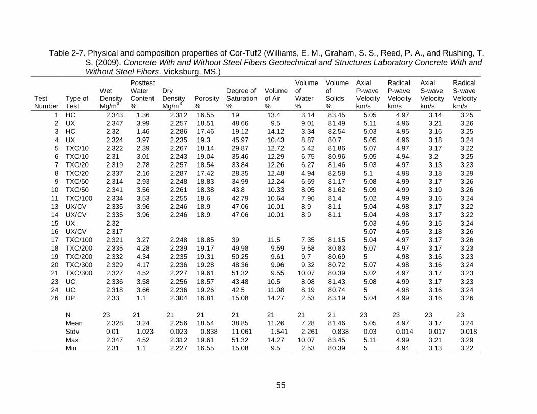
55
Table 2-7. Physical and composition properties of Cor-Tuf2 (Williams, E. M., Graham, S. S., Reed, P. A., and Rushing, T. S. (2009). Concrete With and Without Steel Fibers Geotechnical and Structures Laboratory Concrete With and Without Steel Fibers. Vicksburg, MS.)
Test Number
Type of Test
Wet Density Mg/m
3
Posttest Water Content %
Dry Density Mg/m
3
Porosity %
Degree of Saturation %
Volume of Air %
Volume of Water %
Volume of Solids %
Axial P-wave Velocity km/s
Radical P-wave Velocity km/s
Axial S-wave Velocity km/s
Radical S-wave Velocity km/s
1 HC 2.343 1.36 2.312 16.55 19 13.4 3.14 83.45 5.05 4.97 3.14 3.25
2 UX 2.347 3.99 2.257 18.51 48.66 9.5 9.01 81.49 5.11 4.96 3.21 3.26
3 HC 2.32 1.46 2.286 17.46 19.12 14.12 3.34 82.54 5.03 4.95 3.16 3.25
4 UX 2.324 3.97 2.235 19.3 45.97 10.43 8.87 80.7 5.05 4.96 3.18 3.24
5 TXC/10 2.322 2.39 2.267 18.14 29.87 12.72 5.42 81.86 5.07 4.97 3.17 3.22
6 TXC/10 2.31 3.01 2.243 19.04 35.46 12.29 6.75 80.96 5.05 4.94 3.2 3.25
7 TXC/20 2.319 2.78 2.257 18.54 33.84 12.26 6.27 81.46 5.03 4.97 3.13 3.23
8 TXC/20 2.337 2.16 2.287 17.42 28.35 12.48 4.94 82.58 5.1 4.98 3.18 3.29
9 TXC/50 2.314 2.93 2.248 18.83 34.99 12.24 6.59 81.17 5.08 4.99 3.17 3.26
10 TXC/50 2.341 3.56 2.261 18.38 43.8 10.33 8.05 81.62 5.09 4.99 3.19 3.26
11 TXC/100 2.334 3.53 2.255 18.6 42.79 10.64 7.96 81.4 5.02 4.99 3.16 3.24
13 UX/CV 2.335 3.96 2.246 18.9 47.06 10.01 8.9 81.1 5.04 4.98 3.17 3.22
14 UX/CV 2.335 3.96 2.246 18.9 47.06 10.01 8.9 81.1 5.04 4.98 3.17 3.22
15 UX 2.32
5.03 4.96 3.15 3.24
16 UX/CV 2.317
5.07 4.95 3.18 3.26
17 TXC/100 2.321 3.27 2.248 18.85 39 11.5 7.35 81.15 5.04 4.97 3.17 3.26
18 TXC/200 2.335 4.28 2.239 19.17 49.98 9.59 9.58 80.83 5.07 4.97 3.17 3.23
19 TXC/200 2.332 4.34 2.235 19.31 50.25 9.61 9.7 80.69 5 4.98 3.16 3.23
20 TXC/300 2.329 4.17 2.236 19.28 48.36 9.96 9.32 80.72 5.07 4.98 3.16 3.24
21 TXC/300 2.327 4.52 2.227 19.61 51.32 9.55 10.07 80.39 5.02 4.97 3.17 3.23
23 UC 2.336 3.58 2.256 18.57 43.48 10.5 8.08 81.43 5.08 4.99 3.17 3.23
24 UC 2.318 3.66 2.236 19.26 42.5 11.08 8.19 80.74 5 4.98 3.16 3.24
26 DP 2.33 1.1 2.304 16.81 15.08 14.27 2.53 83.19 5.04 4.99 3.16 3.26
N 23 21 21 21 21 21 21 21 23 23 23 23
Mean 2.328 3.24 2.256 18.54 38.85 11.26 7.28 81.46 5.05 4.97 3.17 3.24
Stdv 0.01 1.023 0.023 0.838 11.061 1.541 2.261 0.838 0.03 0.014 0.017 0.018
Max 2.347 4.52 2.312 19.61 51.32 14.27 10.07 83.45 5.11 4.99 3.21 3.29
Min 2.31 1.1 2.227 16.55 15.08 9.5 2.53 80.39 5 4.94 3.13 3.22

56
Table 2-8. Unconfined compressive strength for Cor-Tuf cylinders (Williams, E. M., Graham, S. S., Reed, P. A., and Rushing, T. S. (2009). Concrete With and Without Steel Fibers Geotechnical and Structures Laboratory Concrete With and Without Steel Fibers. Vicksburg, MS.)
Cor-Tuf1 UC Strength, Mpa Cor-Tuf 2 UC Strength, Mpa
75-by 150-mm Cylinder
100-by 200-mm Cylinder
75-by 150-mm Cylinder Without
Steel Fibers 75-by 100-mm Cylinder
237 216 216 228
231 219 208 225
243 226 206 209
233 228 190
238 229 225
244 209
Table 2-9. Mechanical properties of ultra-high performance cement based composite (UHPCC) (Rong, Z., Sun, W., and Zhang, Y. (2010). “Dynamic compression behavior of ultra-high performance cement based composites.” International Journal of Impact Engineering, Elsevier Ltd, 37(5), 515-520.)
Number Compressive
strength (MPa)
Peak value of strain (x
10-3)
Elastic modulus (GPa)
Toughness index
ηc5 ηc10 ηc30
UHPCC(V0) 143 2.817 54.7 2.43 2.43 2.43
UHPCC(V3) 186 3.857 57.3 3.59 5.08 5.57
UHPCC(V4) 204 4.165 57.9 4.57 6.32 7.39

57
Table 2-10. Slab reinforcement and charge description (Wu, C., Oehlers, D. J., Rebentrost, M., Leach, J., and Whittaker, a. S. (2009). “Blast testing of ultra-high performance fibre and FRP-retrofitted concrete slabs.” Engineering Structures, Elsevier Ltd, 31(9), 2060-2069.)
Blast Slab name
Description Rebar
ratio (%) Standoff
distance (m)
Scaled distance (m/kg1/3)
Explosive mass (g)
NRC-1 1A RC 1.34 3 3 1007 NRC-2 1A RC 1.34 3 1.5 8139 NRC-3 1B RC 1.34 1.4 0.93 3440 NRC-4 1A RC 1.34 1.5 0.75 8213 RET-1a 3A RCCCFRP 1.34 1.5 1.5 1044 RET-2a 3B RCCCFRP 1.34 0.92 0.54 5083 UHPFC D1B UHPFC — 0.75 0.5 3433 RUHPFC D3A RUHPFC 1.34 1 0.37 20101
Table 2-11. Deflections for slabs subject to blast (Wu, C., Oehlers, D. J., Rebentrost, M., Leach, J., and Whittaker, a. S. (2009). “Blast testing of ultra-high performance fibre and FRP-retrofitted concrete slabs.” Engineering Structures, Elsevier Ltd, 31(9), 2060-2069.)
Blast Charge weight
(kg)
Standoff distance from
PT1 (m)
Scaled distance (m/kg1/3)
Max. Deflection
(mm)
Permanent deflection
(mm)
NRC-1 1 3 3 1.5 0
NRC-2 8 3 1.5 10.5 —a
NRC-3 3.4 1.4 0.93 13.9 —a
NRC-4 8 1.5 0.75 38.9 —a
RET-1 1 1.5 1.5 3.3 0
RET-2 5 0.92 0.54 50.6 7.6
UHPFC 3.4 0.75 0.5 13.2 4.1
RUHPFC 20 1 0.37 >100 —b a LVDT debonded from the concrete and the permanent deflection was not recorded.
b LVDT was destroyed by the test.

58
Table 2-12. Properties of steel in Feldman and Siess beams (Feldman, A., and Siess, C. P. (1958). Investigation of Resistance and Behavior of Reinforced Concrete Members Subjected to Dynamic Loading - Part II. Urbana, Illinois.)

59
Table 2-13. Concrete properties for Feldman and Siess beams (Feldman, A., and Siess, C. P. (1958). Investigation of Resistance and Behavior of Reinforced Concrete Members Subjected to Dynamic Loading - Part II. Urbana, Illinois.)

60
Table 2-14. Results for the Habel and Gauvreau drop hammer tests (Habel, K., and Gauvreau, P. (2008). “Response of ultra-high performance fiber reinforced concrete (UHPFRC) to impact and static loading.” Cement and Concrete Composites, Elsevier Ltd, 30(10), 938-946.)
Specimen name (-)
Drop weight
(kg)
Number of drops (-)
First Drop
Max. f1 (mm)
Max. FDW (kN)
Max. FSU (kN)
Max. dε/dt (s-1)
10kg_1 10.3 4 -4.1 23 24.5 2.5 10kg_2 10.3 5 -4.2 23.4 25.3 2.6 10kg_3 10.3 5 -4.6 22.8 26.4 3 10kg_4 10.3 3 -5.1 23.5 18.5 2.4 10kg_5 10.3 3 -5.1 21.6 16.7 2.8 10kg_6 10.3 3 -5.2 21.5 14.8 1.9 10kg_7 10.3 3 -5.7 23.3 20.9 2.7 20kg_1 20.6 2 -6.5 26.3 30.7 2.3 20kg_2 20.6 2 -12.2 23.4 19.7 3.1
20kg_3 20.6 1 —a 23 14.3 3.5
20kg_4 20.6 1 —a 23.8 13.3 3.4
20kg_5 20.6 1 —a 23.8 17.1 3.3
20kg_6 20.6 1 —a 22.8 16.5 2.9 a Not applicable due to complete failure of the specimen at first drop
Table 2-15. Reactive powder concrete (RPC) mix proportions (Fujikake, K., Senga, T.,
Ueda, N., Ohno, T., and Katagiri, M. (2006). “Study on Impact Response of Reactive Powder Concrete Beam and Its Analytical Model.” Journal of Advanced Concrete Technology, 4(1), 99-108.)

61
Figure 2-1. Early age shrinkage in concrete with varying levels of superplasticizer
(Morin, V., Cohen Tenoudji, F., Feylessoufi, a., and Richard, P. (2001). “Superplasticizer effects on setting and structuration mechanisms of ultrahigh-performance concrete.” Cement and Concrete Research, 31(1), 63-71.)
Figure 2-2. Compressive strength curve with the addition of fibers (Fehling, E., Bunje, K., and Leutbecher, T. (2004). “Design relevant properties of hardened Ultra High Performance Concrete.” International Symposium on Ultra High Performance Concrete, Kassel, Germany, 327-338.)

62
Figure 2-3. Tensile strength curve with the addition of fibers (Fehling, E., Bunje, K., and
Leutbecher, T. (2004). “Design relevant properties of hardened Ultra High Performance Concrete.” International Symposium on Ultra High Performance Concrete, Kassel, Germany, 327-338.)
Figure 2-4. Impact performance of normal-strength polymer macro-FRC (PFRC)
(Bindiganavile, V., Banthia, N., and Aarup, B. (2002). “Impact Response of Ultra-High-Strength Fiber-Reinforced Cement Composite.” ACI Materials Journal, (99-M55), 543-548.)

63
Figure 2-5. Impact performance of normal-strength steel FRC (SFRC) (Bindiganavile,
V., Banthia, N., and Aarup, B. (2002). “Impact Response of Ultra-High-Strength Fiber-Reinforced Cement Composite.” ACI Materials Journal, (99-M55), 543-548.)
Figure 2-6. Fiber protrusion from cracked beam (Kang, S., Lee, Y., Park, Y., and Kim, J.
(2010). “Tensile fracture properties of an Ultra High Performance Fiber Reinforced Concrete (UHPFRC) with steel fiber.” Composite Structures, Elsevier Ltd, 92(1), 61-71.)

64
Figure 2-7. Dramix ZP305 Fiber (Williams, E. M., Graham, S. S., Reed, P. A., and
Rushing, T. S. (2009). Concrete With and Without Steel Fibers Geotechnical and Structures Laboratory Concrete With and Without Steel Fibers. Vicksburg, MS.)
Figure 2-8. Bending tensile stress versus deflection for heat treated and water cured
concrete (Rossi, P., Arca, A., Parant, E., and Fakhri, P. (2005). “Bending and compressive behaviours of a new cement composite.” Cement and Concrete Research, 35(1), 27-33.)

65
Figure 2-9. Typical ultra-high performance fiber reinforced concrete (UHPFRC) strength
characteristics (Wu, C., Oehlers, D. J., Rebentrost, M., Leach, J., and Whittaker, a. S. (2009). “Blast testing of ultra-high performance fibre and FRP-retrofitted concrete slabs.” Engineering Structures, Elsevier Ltd, 31(9), 2060-2069.)
Figure 2-10. (a) Three-point bending test setup; (b) Four-point bending test setup
(Habel, K., and Gauvreau, P. (2008). “Response of ultra-high performance fiber reinforced concrete (UHPFRC) to impact and static loading.” Cement and Concrete Composites, Elsevier Ltd, 30(10), 938-946.)

66
Figure 2-11. Three-point bending results (Habel, K., and Gauvreau, P. (2008). “Response of ultra-high performance fiber reinforced concrete (UHPFRC) to impact and static loading.” Cement and Concrete Composites, Elsevier Ltd, 30(10), 938-946.)
Figure 2-12. Four-point bending results (Habel, K., and Gauvreau, P. (2008). “Response of ultra-high performance fiber reinforced concrete (UHPFRC) to impact and static loading.” Cement and Concrete Composites, Elsevier Ltd, 30(10), 938-946.)

67
Figure 2-13. UHPFRC moment-curvature relationship (Habel, K., and Gauvreau, P.
(2008). “Response of ultra-high performance fiber reinforced concrete (UHPFRC) to impact and static loading.” Cement and Concrete Composites, Elsevier Ltd, 30(10), 938-946.)
Figure 2-14. Triaxial pressure vessel (Williams, E. M., Graham, S. S., Reed, P. A., and
Rushing, T. S. (2009). Concrete With and Without Steel Fibers Geotechnical and Structures Laboratory Concrete With and Without Steel Fibers. Vicksburg, MS.)

68
Figure 2-15. Stress-strain for unconfined compression (UC) test of Cor-Tuf1 (Williams,
E. M., Graham, S. S., Reed, P. A., and Rushing, T. S. (2009). Concrete With and Without Steel Fibers Geotechnical and Structures Laboratory Concrete With and Without Steel Fibers. Vicksburg, MS.)
Figure 2-16. Stress-strain for UC test of Cor-Tuf2 (Williams, E. M., Graham, S. S.,
Reed, P. A., and Rushing, T. S. (2009). Concrete With and Without Steel Fibers Geotechnical and Structures Laboratory Concrete With and Without Steel Fibers. Vicksburg, MS.)

69
Figure 2-17. Triaxial compression (TXC) test results with confining pressures of 10MPa
to 300 MPa (Cor-Tuf1) (Williams, E. M., Graham, S. S., Reed, P. A., and Rushing, T. S. (2009). Concrete With and Without Steel Fibers Geotechnical and Structures Laboratory Concrete With and Without Steel Fibers. Vicksburg, MS.)
Figure 2-18. TXC test results with confining pressures of 10MPa to 300 MPa (Cor-Tuf2) (Williams, E. M., Graham, S. S., Reed, P. A., and Rushing, T. S. (2009). Concrete With and Without Steel Fibers Geotechnical and Structures Laboratory Concrete With and Without Steel Fibers. Vicksburg, MS.)

70
Figure 2-19. Stress path from direct pull tests for Cor-Tuf1 (Williams, E. M., Graham, S.
S., Reed, P. A., and Rushing, T. S. (2009). Concrete With and Without Steel Fibers Geotechnical and Structures Laboratory Concrete With and Without Steel Fibers. Vicksburg, MS.)
Figure 2-20. Stress path from direct pull tests for Cor-Tuf2 (Williams, E. M., Graham, S.
S., Reed, P. A., and Rushing, T. S. (2009). Concrete With and Without Steel Fibers Geotechnical and Structures Laboratory Concrete With and Without Steel Fibers. Vicksburg, MS.)

71
Figure 2-21. Block-bar device diagram (Parant, E., Rossi, P., Jacquelin, E., and Boulay,
C. (2007). “Strain Rate Effect on Bending Behavior of New Ultra-High- Performance Cement-Based Composite.” ACI Materials Journal, (104-M50), 458-463.)
Figure 2-22. Modulus of Rupture-stress rate diagram (Parant, E., Rossi, P., Jacquelin,
E., and Boulay, C. (2007). “Strain Rate Effect on Bending Behavior of New Ultra-High- Performance Cement-Based Composite.” ACI Materials Journal, (104-M50), 458-463.)

72
Figure 2-23. Uniaxial tensile stress vs. stress rate (Parant, E., Rossi, P., Jacquelin, E.,
and Boulay, C. (2007). “Strain Rate Effect on Bending Behavior of New Ultra-High- Performance Cement-Based Composite.” ACI Materials Journal, (104-M50), 458-463.)
Figure 2-24. Dynamic increase factor (DIF) vs. strain rate (Ngo, T., Mendis, P., and
Krauthammer, Ted. (2007). “Behavior of Ultrahigh-Strength Prestressed Concrete Panels Subjected to Blast Loading.” Journal of Structural Engineering, ASCE, (November), 1582-1590.)

73
Figure 2-25. Stress-strain diagrams for split-hopkinson pressure bar (SHPB) tests with
varying fiber percentages (Rong, Z., Sun, W., and Zhang, Y. (2010). “Dynamic compression behavior of ultra-high performance cement based composites.” International Journal of Impact Engineering, Elsevier Ltd, 37(5), 515-520.)
Figure 2-26. SHPB specimens post-test (Rong, Z., Sun, W., and Zhang, Y. (2010).
“Dynamic compression behavior of ultra-high performance cement based composites.” International Journal of Impact Engineering, Elsevier Ltd, 37(5), 515-520.)
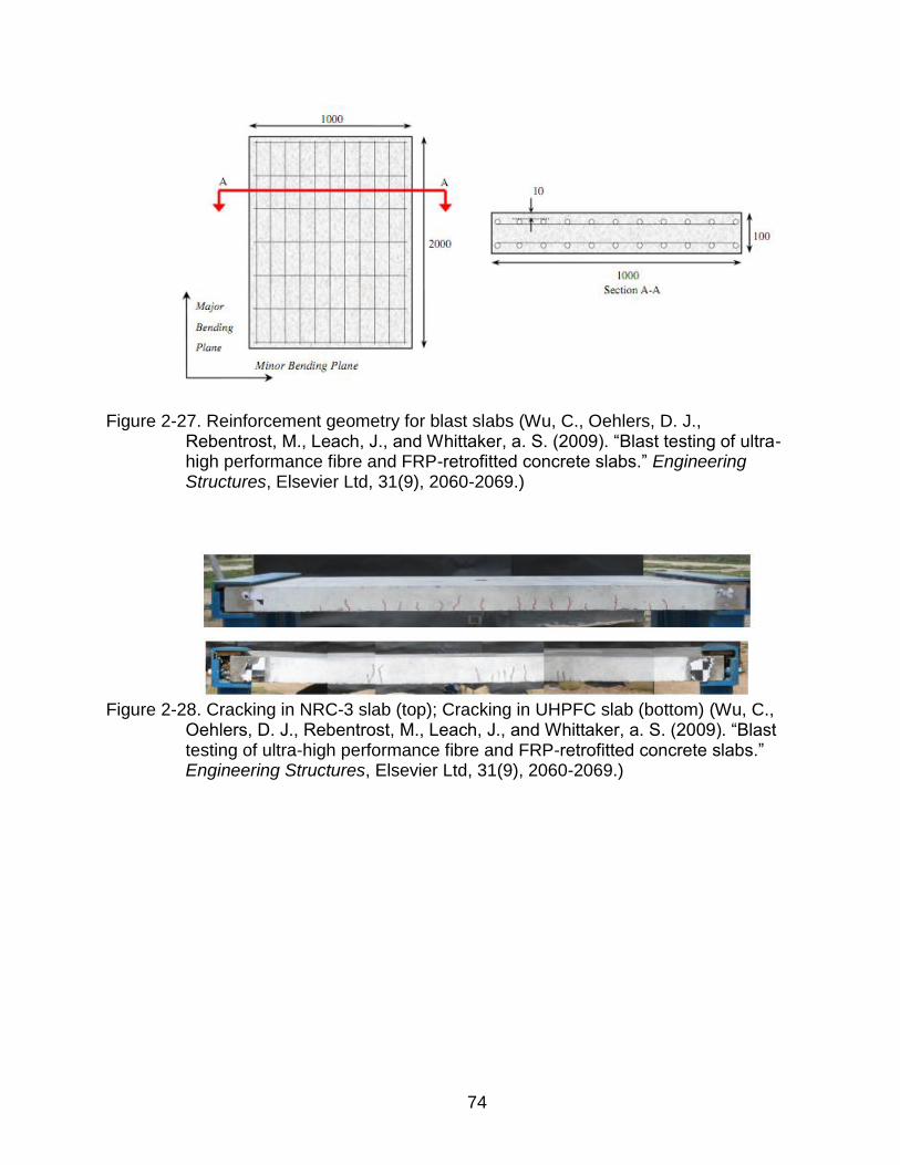
74
Figure 2-27. Reinforcement geometry for blast slabs (Wu, C., Oehlers, D. J., Rebentrost, M., Leach, J., and Whittaker, a. S. (2009). “Blast testing of ultra-high performance fibre and FRP-retrofitted concrete slabs.” Engineering Structures, Elsevier Ltd, 31(9), 2060-2069.)
Figure 2-28. Cracking in NRC-3 slab (top); Cracking in UHPFC slab (bottom) (Wu, C.,
Oehlers, D. J., Rebentrost, M., Leach, J., and Whittaker, a. S. (2009). “Blast testing of ultra-high performance fibre and FRP-retrofitted concrete slabs.” Engineering Structures, Elsevier Ltd, 31(9), 2060-2069.)

75
Figure 2-29. Feldman and Siess reinforced concrete beam design, front view (Feldman, A., and Siess, C. P. (1956). Investigation of Resistance and Behavior of Reinforced Concrete Members Subjected to Dynamic Loading - Part I. Urbana, Illinois.)
Figure 2-30. Feldman and Siess beam 1-f and 1-h, section view (Adapted from Feldman, A., and Siess, C. P. (1956). Investigation of Resistance and Behavior of Reinforced Concrete Members Subjected to Dynamic Loading - Part I. Urbana, Illinois.)

76
Figure 2-31. Load vs. Midspan Displacement for Feldman and Siess static tests (Feldman, A., and Siess, C. P. (1958). Investigation of Resistance and Behavior of Reinforced Concrete Members Subjected to Dynamic Loading - Part II. Urbana, Illinois.)

77
Figure 2-32. Load time-history for Feldman and Siess Beam 1-f (Feldman, A., and Siess, C. P. (1958). Investigation of Resistance and Behavior of Reinforced Concrete Members Subjected to Dynamic Loading - Part II. Urbana, Illinois.)
Figure 2-33. Load-beam system for single degree of freedom (SDOF) calculations
(Feldman, A., and Siess, C. P. (1956). Investigation of Resistance and Behavior of Reinforced Concrete Members Subjected to Dynamic Loading - Part I. Urbana, Illinois.)

78
Figure 2-34. Displacement vs. time for impact of Beam 1H (Feldman, A., and Siess, C.
P. (1958). Investigation of Resistance and Behavior of Reinforced Concrete Members Subjected to Dynamic Loading - Part II. Urbana, Illinois.)

79
Figure 2-35. Habel and Gauvreau drop hammer setup (Habel, K., and Gauvreau, P.
(2008). “Response of ultra-high performance fiber reinforced concrete (UHPFRC) to impact and static loading.” Cement and Concrete Composites, Elsevier Ltd, 30(10), 938-946.)
Figure 2-36. Two mass-spring model (Habel, K., and Gauvreau, P. (2008). “Response
of ultra-high performance fiber reinforced concrete (UHPFRC) to impact and static loading.” Cement and Concrete Composites, Elsevier Ltd, 30(10), 938-946.)

80
Figure 2-37. (a) Drop weight force vs. time; (b) Deflection vs. time (Habel, K., and
Gauvreau, P. (2008). “Response of ultra-high performance fiber reinforced concrete (UHPFRC) to impact and static loading.” Cement and Concrete Composites, Elsevier Ltd, 30(10), 938-946.)
Figure 2-38. Fujikake et al. reactive powder concrete (RPC) beam cross section (Fujikake, K., Senga, T., Ueda, N., Ohno, T., and Katagiri, M. (2006). “Study on Impact Response of Reactive Powder Concrete Beam and Its Analytical Model.” Journal of Advanced Concrete Technology, 4(1), 99-108.)

81
Figure 2-39. Fujkake et al. drop hammer test setup (Fujikake, K., Senga, T., Ueda, N., Ohno, T., and Katagiri, M. (2006). “Study on Impact Response of Reactive Powder Concrete Beam and Its Analytical Model.” Journal of Advanced Concrete Technology, 4(1), 99-108.)
Figure 2-40. (a) Fujikake et al. drop hammer test from 0.8 m; (b) Drop from 1.2 m (Fujikake, K., Senga, T., Ueda, N., Ohno, T., and Katagiri, M. (2006). “Study on Impact Response of Reactive Powder Concrete Beam and Its Analytical Model.” Journal of Advanced Concrete Technology, 4(1), 99-108.)

82
Figure 2-41. Flow process for a physical problem solved with finite element analysis (Bathe, K. (1995). Finite Element Procedures. Prentice-Hall, Upper Saddle River, New Jersey.)

83
3 CHAPTER 3 EXPERIMENTAL INVESTIGATION
3.1 Introduction
The majority of the experimental portion of this project will take place after the
completion of this paper; however, the magnitude of the experiments will be based on
the predictions made during the numerical analysis discussed later on. The static beam
test results, which have been obtained for all 6 beam series, will be presented in
conjunction with the simulated results along with discussion. The following is a
description of the specimens and equipment that will be utilized to statically and
dynamically characterize the properties of Cor-Tuf. All of the NSC and Cor-Tuf beam
and cylinder specimens were mixed, poured and cast from the same mix batches to
ensure uniformity during testing. The data gathered from these experiments will be
utilized to calibrate the prediction models and create accurate material models.
3.2 Test Specimens
3.2.1 Cylinders For Static Tests
The Geotechnical and Structures Laboratory, ERDC, US Army, was responsible
for specimen preparation and static testing of all 6 in diameter by 12 in height
specimens. ERDC retained 9 of these cylinders to statically test as none of the
equipment at the University of Florida can generate enough force to test the UHPC
cylinders. These cylinders are indicated in Table 3-1. The Center for Infrastructure
Protection and Physical Security at the University of Florida (CIPPS) will test the 4 in
diameter by 8 in height (4x8) specimens locally to accelerate the testing process. For
static testing purposes a total of 9 - 4x8 cylinders will be produced by ERDC and tested.
The specimen quantities and materials for static tests are summarized in Table 3-2.

84
3.2.2 Cylinders For Dynamic Tests
The cylinders for dynamic testing, also prepared by ERDC, will be tested at
CIPPS. ERDC will cast, in addition to the static cylinders already mentioned, 9 – 4 in
diameter by 8 in tall cylinders for impact testing as shown in Table 3-3. Additionally, 99
cylinders will be cast in addition to the static cylinders in the 6 in diameter by 12 in
height size, see Table 3-4. The variation in sizes will allow for a first impression of any
size effects in Cor-Tuf.
3.2.3 Beams For Static and Impact Testing
In addition to cylinder testing, a series of beams constructed of NSC as well as
both variations of Cor-Tuf will be tested both statically and dynamically at CIPPS. The
Geotechnical and Structures Laboratory at ERDC will also cast the beams. The beams
will be cast from the same concrete batches as the cylinders and subjected to the same
curing process. This will ensure that the cylinders can provide specific characteristic
curves to the material used in the beams.
Typical beam dimensions, reinforcement details, and cross sections are shown in
Figure 3-1 and described in Table 3-5 and Table 3-6. All reinforcement except the B5
series shall be Grade 60. The B5 series will be made of Cor-Tuf1 without reinforcing
bars. The B2 and B6 series will only contain longitudinal reinforcement, no shear
reinforcement (stirrups). This specimen design was created after the discovery of the
findings in Graybeal (2005) which showed that UHPC with fibers reinforcement may not
require shear reinforcement. In each specimen, a 1 in thick steel plates shall be placed
at support points and ½ in thick steel plate at load point. The plates should help avoid
any issues of localized crushing. Strain gages will be placed along both of the tension
(bottom) reinforcement bars at 18 in spacing (3 per reinforcing bar) for each beam

85
specimen before the casting of concrete, and the strain gage calibration data will be
provided to CIPPS including the conversion to strain and the initial bias. The six strain
gages will be placed at each of the quarter-spans (two per end per bar) as well as at the
midspan (two) of the bottom rebar.
3.3 Testing Equipment and Setup
3.3.1 Static Testing Equipment For Cylinders
The first set of static tests were performed on cylinders measuring 4” x 8” and will
be performed locally at the University of Florida in Weil Hall using a Gilson MC-250CS
compression testing unit, shown in Figure 3-4. The capacity of this machine is 350 klbf
however it does not have any output for the load applied and therefore will not be used
for the 4” x 8” Cor-Tuf cylinders. Additionally, the 6” x 12” cylinders require over 700 kips
of force and will need to be tested at FDOT. The first tests conducted with the 4” x 8”
cylinders were not from the beam concrete batches and were merely for calibration
purposes. The cylinders were not outfitted with strain gages, subsequent tests will
contain significant amounts of data and will measure the post-peak behavior of all three
materials for use in accurate modeling of the cylinders and beams.
The 4” x 8” and 6” x 12” cylinder tests will be conducted on 3 cylinders of each
material at FDOT. If possible, the tests will be carried out with the same strain gage
pattern. The tests will help calibrate the models as well as create a control group for the
dynamic tests. The dynamic tests will attempt to use the same strain gage patterns as
well.
3.3.2 Static Testing Equipment For Beams
Static testing of beams will be accomplished with the use of an Enerpac RC-5013
hydraulic jack controlled by an Enerpac P-462 hand pump with an oil pressure gauge.

86
The load will be slowly applied to the beam in 1-2 kip increments to ensure that the
failure can be properly captured. In between each increment, loading will be paused and
the beam will checked for cracking and any other irregularities. The data acquisition
(DAQ) for this portion of the testing will be recorded using a National Instruments USB-
6218 capable of recording 32 analog channels of 16 bits at 250 kS/s
(kilosamples/second). A special program was created to run the NI DAQ that allowed for
sampling of each signal at 100-1000 Hz during loading, and then at a rate of 0.5 Hz
while hand measurements were being taken.
3.3.3 Dynamic Testing Equipment For Cylinders
Dynamic testing of cylinders will be carried out using the CIPPS drop hammer
shown in Figure 3-6. Table 3-7 describes the specific measurements and capabilities of
the drop hammer. The hammer can release its maximum weight of approximately 600
lbs, when outfitted with a load cell and striker plate, from a height of over 16 feet. Drops
from this height, depending on the response of the specimen, can create forces
exceeding 1000 kips, although for no longer than 0.5-2 milliseconds. However, despite
this great force, the possibility exists that it may not be capable of failing all of the test
specimens, especially the cylinders. For this reason, extra load plates have been
manufactured to create a higher impact load. This will be discussed further in the
chapter on numerical predictions. An important aspect to note about the hammer is its
braking system. The brakes are designed to deploy after the load cell reaches a certain
load. The brakes will fire and as the load cart is rebounding off of the beam or cylinder,
stop it from contacting the specimen a second time. In this way, any specimen that has
been subjected to an impact load can be tested further if it has not failed.

87
3.3.4 Dynamic Testing Equipment For Beams
The beams will be tested in much the same manner as the cylinder using the
impact drop hammer. The beams will be supported on each end with a stand that is
attached to the strong floor of the laboratory. Each stand is constructed with a roller to
allow for simply supported conditions as well as a load cell mounted below the roller to
capture the reactions from the tests. An example of the supports can be seen in
3.4 Instrumentation
The data from testing of the cylinders and beams will be both thorough and
complex. The data acquisition system utilized for the static and dynamic testing of
beams, and the dynamic testing of cylinders is shown in Figure 3-7. The system
consists of a High Techniques HT600 to capture the voltages of all incoming signals; an
OASIS 2000 signal conditioner to condition raw voltage and supply voltage to strain
gauges and load cells; and a rack computer to save all of the incoming data as well as
monitor the tests in progress. The HT600 contains 64 channels that read from BNC
cables. Each channel is read independently in order for the data to be read
continuously. The channels can each hold up to 8 million points that can be read up to a
frequency of 2 million points per second. The OASIS 2000 is setup with 10 boards
capable of regulating the voltage to load cells and strain gages. Additionally, it is set up
with 2 boards that are capable of supplying current to accelerometers and other sensors
that require it. The OASIS 2002 is capable of outputting 5,10 and 15 V at gains of 1-
1000.
The instrumentation that will be monitored by the data acquisition systems
includes all of the following: strain gages of varying sizes on both concrete and steel
inside of the beams, accelerometers, displacement gauges, velocity sensors and load

88
cells ranging from 50 kips to 2000 kips. The data from these inputs can be sampled at
frequencies of up to 2 MHz which will be vital for dynamic tests that will not exceed 5
ms. The tests will also be captured by both normal and high speed video. The high
speed cameras utilized will be a Memrecam fx K3 high speed camera as well as a
Phantom v5.2. The Memrecam is capable of capturing footage at 10,000 fps at a
resolution of 1280 x 96. The Phantom camera is capable of capturing video at 148,000
fps at a resolution of 96 x 8 (although at this resolution the captured footage will likely
not be useful).

89
Table 3-1. 6” x 12” cylinder quantities and material properties for static testing
Series Quantity Size Material
1S-6x12 3 6”x12” NSC (f’c = 3500 psi) 2S-6x12 3 6”x12” Cor-Tuf with fibers (Cor-Tuf1) 3S-6x12 3 6”x12” Cor-Tuf without fibers (Cor-Tuf2)
Table 3-2. 4” x 8” cylinder quantities and material properties for static testing
Series Quantity Size Material
1S-4x8 3 4”x8” NSC (f’c = 3500 psi) 2S-4x8 3 4”x8” Cor-Tuf with fibers (Cor-Tuf1) 3S-4x8 3 4”x8” Cor-Tuf without fibers (Cor-Tuf2)
Table 3-3. 4” x 8” cylinder quantities and material properties for impact testing
Series Quantity Material
1D-4x8* 3 NSC (f’c = 3500 psi) 2D-4x8* 3 Cor-Tuf with fibers (Cor-Tuf1) 3D-4x8* 3 Cor-Tuf without fibers (Cor-Tuf2)
*Use the same concrete, as for the cylinders in Table 3-1 and Table 3-2
Table 3-4. 6” x 12” cylinder quantities and material properties for impact testing
Series Quantity Material
1D-6x12* 33 NSC (f’c = 3500 psi) 2D-6x12* 33 Cor-Tuf with fibers (Cor-Tuf1) 3D-6x12* 33 Cor-Tuf without fibers (Cor-Tuf2)
*Use the same concrete, as for the cylinders in Table 3-1 and Table 3-2
Table 3-5. Beam quantities and materials for static and impact testing
Series Quantity Materials
Details Concrete
Longitudinal Reinforcement
Shear Reinforcement
B1 6 NSC (f’c = 3500 psi) Top 2-#6
Bottom 2#7 #3 @ 5”
Fig.1
B2 2 NSC (f’c = 3500 psi) Top 2-#6
Bottom 2#7 No shear
Reinforcement Fig. 2
B3 6 Cor-Tuf with fibers (Cor-Tuf1)
Top 2-#6 Bottom 2#7
#3 @ 5” Fig. 1
B4 6
Cor-Tuf without fibers (Cor-Tuf2)
Top 2-#6 Bottom 2#7
#3 @ 5” Fig. 1
B5 6 Cor-Tuf with fibers (Cor-Tuf1)
No longitudinal reinforcement
No shear Reinforcement
Fig. 3
B6 6 Cor-Tuf with fibers (Cor-Tuf1)
Top 2-#6 Bottom 2#7
No shear Reinforcement
Fig. 2

90
Table 3-6. Static and impact testing matrix per material
Test Quantity Description
Static 1 Static displacement controlled test for obtaining the resistance function.
Impact 1 Multiple drops with increasing drop heights in on the same specimen till failure.
Impact 3 Single drop height high enough to cause failure in the specimen. (Not carried out for B2)
*With the exception of series B2, all series will have one extra beam as a precaution.
Table 3-7. Center for Infrastructure Protection and Physical Security (CIPPS) Drop Hammer Specifications
Drop Hammer Specifications
Rail Cart Weight 129.46 lbs
Adapter Plates Total 365.00 lbs
Striker Weight Varying
Drop Tower Height 195.84 in
Minimum Drop Height 12 in

91
Section A-A Section B-B Section C-C
Figure 3-1. Beam dimensions and details for series B1, B3 and B4 (Table 3-5)

92
Section A-A Section B-B Section C-C
Figure 3-2. Beam dimensions and details for series B2 and B6 (Table 3-5)

93
Section A-A Section B-B Section C-C
Figure 3-3. Beam dimensions and details for series B5 (Table 3-5)

94
Figure 3-4. Gilson MC-250CS Compression Testing Machine
Figure 3-5. Enerpac RC-5013 hydraulic jack for static testing

95
Figure 3-6. Center for Infrastructure Protection Physical Security (CIPPS) Drop Hammer

96
Figure 3-7. CIPPS Data Acquisition System

97
Figure 3-8. Supports for beam testing

98
4 CHAPTER 4 MODEL VALIDATION
4.1 Introduction
The Feldman and Siess impact experiments (Feldman and Siess 1956, 1958)
were utilized as the validation cases for the numerical modeling performed in this
project. The beam design created by Feldman and Siess, and replicated for these
experiments, is well suited due to both the size of the beams as well as the
reinforcement detail utilized. While modifications in the type of steel, and strength of the
concrete and steel were made for the final beams to be tested, the overall design and
shape remained the same. In addition the beams having the desired properties for
testing, the documentation of the experimental work also allowed for accurate model
validation.
This chapter contains the model validation work that was completed and utilized to
create the predictions for the CIPPS beam specimens that will be tested. The following
items will be covered in this chapter: material models, inputs for Abaqus parameters,
modeling details and the results of the models compared to experimental results. While
the models did not fully capture the results of the Feldman and Siess experiments, the
overall behavior of each experiment was properly presented in the models.
4.2 Material Models
A variety of material models exists for both concrete and steel depending on both
the types of concrete and steel and the interaction between the two. For the purposes of
the numerical solutions shown here, the modified Hognestad parabola (MacGregor and
Wight 2005) concrete model was utilized for concrete in compression. The Hognestad
parabola utilizes the compressive strength from cylinder tests as well as common

99
parameters for normal strength concrete to create a characteristic material curve.
Modifications were made to the curve to accommodate the methodologies of Abaqus.
The tension portion of the concrete model was based on the Hsu model (Hsu 1993) for
concrete in tension. This model was chosen as it closely follows the ACI
recommendations (American Concrete Institute 2011). The steel model was based on
the Park and Paulay model described in Park and Paulay (1975). These models have
been tested and utilized in a variety of theses, the most recent being that of Koh (2011),
the material models work well for both static and dynamic scenarios.
4.2.1 Modified Hognestad Parabola
The modified Hognestad parabola utilizes the compression results from a uniaxial
compression test of plain concrete cylinders (6 inch diameter by 12 inch height) to
create material curves. Hognestad created generalized material curves (MacGregor and
Wight 2005) for varying compressive strengths shown in Figure 4-1. The modified
Hognestad stress-strain curve, shown in Figure 4-2, is designed for use with concrete
mixes that do not exceed 6000 psi. In the case of Feldman and Siess the mixes
reached up to 6600 psi but this was deemed within range of the curves predictions. The
curve begins with a second degree parabola that peaks at fc” followed by a linear
descent until a strain of 0.0038.
Parabola:
2
00
" 2
cc
cc ff For 0 c (4-1)
Linear descent:

100
0" ccdcc Eff For 0038.00 thanlessandc (4-2)
With:
cc ff '"9.0
(4-3)
c
c
E
f"
0
8.1
(4-4)
ccc fwE '335.1
For 33 /160/90 ftlbwftlb c (4-5)
cc fE '57000
for normal weighted concrete with cf ' in psi (4-6)
ksiorf
E ccd 500
0038.0
"15.0
0
(4-7)
Where:
cf is the concrete compressive stress.
cf is the maximum concrete compressive stress.
cf ' is the uniaxial concrete compressive strength under standard test cylinder.
c is the concrete strain.
0 is the concrete strain at maximum compressive stress.
cE is the elastic modulus, defined by ACI 318 (2011).
cdE is the descending elastic modulus ACI 318 (2011).
cw is the density of the concrete in lb/ft3.
These equations were utilized to create the compressive curve for concrete that
was inputted into Abaqus’s concrete damage plasticity model, discussed below. A small
modification was necessary in order to meet the requirement of Abaqus. In Abaqus, for
a material to fail, the final strain point must bring the stress below 5% of the maximum

101
stress; otherwise it assumes that the final stress-strain point continues at the same
stress infinitely. For example, from Figure 4-2, the stress would remain at 0.85
cf until
the model completed its run. One of the concrete curves utilized in Abaqus is the one
shown in Figure 4-3, as can be seen the stress drops to 1% of the peak stress allowing
for a failure of the material, but not to zero as this can cause issues in the matrix
calculations resulting in abnormal model failures.
4.2.2 Hsu Tension Model
ACI 318 (2011) Section 8.6.1 recommends that the average splitting tensile
strength be cct ff '7.6 for normal strength concrete, where cf ' is in psi. In Section
9.5.2.3 the modulus of rupture is defined as cr ff '5.7 where cf ' is again in psi.
Clearly, the tensile strength will be far lower than the compressive strength. Despite a
loss in strength following the cracking of the concrete, the tensile strength does not drop
to zero as can be seen in Figure 4-4. While a variety of material models exist, the Hsu
(1993) tension model has provided accurate results in Abaqus models Koh (2011). Hsu
described the tensile stress-strain curve of concrete as seen below:
Ascent:
ccc Ef For crc (4-8)
cc fE '47000
(4-9)
Descent:
002.01 crc
cr
c
ff
(4-10)

102
ccr ff '75.3
(4-11)
Where, as before, cf ' is the uniaxial concrete cylinder compressive strength in psi.
crf is the cracking stress of plain concrete in psi.
cr is the cracking strain.
For similar reasons to that of the compressive strength curves, the tensile curve
that were utilized for input in Abaqus needed to be modified slightly to create a failure
point. In order to accomplish this, the tensile strength was brought to a final stress that
was 5% of the peak tensile strength. The existing curve was extended linearly after
flattening out to a strain of 0.1 to coincide with the failure of the steel reinforcement. An
example of a tensile curve, which is based on a concrete with a compressive strength of
6150 psi, can be seen in Figure 4-5. Although it is not visible, the tensile strength rises
suddenly and then begins decreasing in the curve shown.
4.2.3 Park and Paulay Steel Model
In their book on reinforced concrete, Park and Paulay (1975) present a steel
model based on the principles of strain-hardening. The model consists of an elastic
region, a yield plateau region and a strain hardening region as can be seen in Figure
4-6. The following are the equations utilized to create the characteristic curve:
Region AB:
sss Ef For )( ys (4-12)
Region BC:
ys ff For )( shsy (4-13)
Region CD:

103
])130(2
)60)((
2)(60
2)([
2
r
m
mff
shs
shs
shs
ys
For )( shsy (4-14)
Where:
2
2
15
160)130)((
r
rrf
f
my
u
(4-15)
shsur (4-16)
And:
su is the ultimate strain.
uf is the ultimate stress.
m and r are variables of the equation.
yf is the yield strength of the steel.
sf is the compressive stress at a point on the curve.
sE is the modulus of elasticity for the steel.
sh is the strain when strain hardening begins.
s is the stain at a point on the curve.
As was the case with the other material models, the final stress value was brought
below 10%, in this case 1%, of the peak stress value. The reduction to 1% was chosen
after model validations still showed residual strength with higher values that did not exist
in the experimental results.

104
4.3 Abaqus Parameters
The Abaqus software provides the user with an abundance of options to choose
from for modeling a variety of scenarios. For this reason, the modeling choices that the
user makes must be concise in order to properly capture the behavior of the problem
that needs to be solved. The following section will present some of the choices made for
the model validation and experimental investigation, and why they were chosen.
Additionally, specific modeling intricacies will be discussed that enabled faster modeling
of the specimens and ensured accuracy despite not utilizing all of the physical attributes
of the test, i.e. support conditions.
4.3.1 Concrete Damage Plasticity Model
While three material models exist that are specifically designed to model concrete
in Abaqus, the work presented will utilized the concrete damage plasticity (CDP) model.
Koh (2011) utilized this material model to accurately predict the results of connections
under progressive collapse. The CDP material model is a plasticity-based model
available in Abaqus/Standard and Abaqus/Explicit and can model concrete under
monotonic, cyclic and/or dynamic loading.
The CDP model was selected because of its versatility and ability to run in
Abaqus/Explicit, allowing for the modeling of highly dynamic experiments. The model
uses concepts of isotropic damage elasticity in conjunction with isotropic tensile and
compressive plasticity to represent the inelastic behavior of concrete. The model can
also be defined for sensitivity to the strain rate, including the ability to increase peak
strength at higher strain rates. The model allows for different yield strength in tension
and compression as well as different degradation of the elastic stiffness in tension and
compression.

105
Thus, the model allows for two material curves, the compression curve shown in
Figure 4-7; and the tension curve, shown in Figure 4-8. The compression curve consists
of a linear-elastic (undamaged) section that continues until reaching the stress co ; this
section has a slope of oE , the elastic Young’s modulus. The following section is a curve
that constitutes the start of the plastic region which reaches a peak at the ultimate
stress, cu , after which the stress decreases along the same path. The curve follows a
similar path to that of the modified Hognestad parabola which aids in the input of the
material properties. The tension curve for the CDP model begins in a similar fashion,
with a slope of oE rising until it reaches the tensile failure stress, to . Following this
section, the stress reduces as tension stiffening rules the post-peak behavior. Tension
stiffening accounts for the interaction between concrete and steel by representing the
behavior of both through average strain and average stress throughout the cracked
region. In order for the CDP model to function properly, the tension stiffening region
must be properly defined. Abaqus recommends a linear degradation from the peak
stress until reaching zero at the ultimate strain, however, the method described in
section Hsu Tension Model will be utilized to better approximate the tension stiffening
effect.
An important feature of the CDP model is the damage parameters for both the
concrete and tension portions of the concrete model. The damage is designed to define
the behavior of the material after being loaded and unloaded (cyclic loading). Loading
beyond the elastic range in either compression or tension will lead to a decrease in
strength and stiffness that must be accounted for. The following two damage
parameters, cd and td , define the damage for compression and tension respectively.

106
The values for these damage parameters range from zero, no damage, up to one,
complete damage and loss of all strength.
The stress-strain relationship for the compression curve after reaching peak stress
can be defined in terms of stress and the inelastic (crushing) strain, in
c . The inelastic
strain is calculated as follows:
el
occ
in
c (4-17)
0E
cel
oc
(4-18)
Where:
el
oc is the elastic compressive strain.
c is the total compressive strain.
c is the concrete compressive stress.
0E is the elastic Young’s modulus.
Abaqus takes the inelastic strain values and converts them to plastic strain values,
pl
c . Equation (4-19) shows how the plastic strain values are calculated, these values
must always be positive.
o
c
c
cin
c
pl
cEd
d
1
(4-19)
For the tension behavior, the failure is characterized by the post failure stress and
cracking strain, ck
t
~
. The cracking strain is defined by using the equations below:
el
ott
ck
t ~
(4-20)

107
0E
tel
ot
(4-21)
100
tot
(4-22)
Where:
t is the total strain.
el
ot is elastic strain.
to is the tensile failure/cracking stress.
t is the concrete tensile stress, defined by in Equation (4-22) from Abaqus as the
lower limit of post failure stress, this is to reduce potential numerical problems.
As in the compression curve, the cracking strain values are converted into plastic
strain values, pl
t , using the equation below.
o
t
t
tckt
pl
tEd
d
1
~
(4-23)
In order to calculate the damage parameters for a specific concrete, cyclic loading
tests must be performed on concrete samples, such as concrete cylinders. The tests
performed by Feldman and Siess (1958) did not include cyclic loading tests of the
batches of concrete utilized to create the experimental beams. While it is possible to
utilize the peak compressive stress and some of the mix properties to find a comparable
mix that has been cyclically loaded, it was deemed impractical as even minor changes
in the material properties could adversely affect the damage results. Without having
been present for the Feldman and Siess experiments, the specific mixing and curing
practices can never be known. Therefore, a linear damage model was created for both

108
compression and tension. The compression damage begins at the yield point and
continues to 0.004 total strain reaching a damage value of 0.6. Any value higher than
this yielded a negative plastic strain. Similarly, the tension damage begins at the
cracking strain with a value of 0 and ends at a value of 0.95 damage at 0.1 total strain.
In addition to the compression and tension characteristic curves and their
respective damage parameters, the CDP model also contains a set of parameters to
further control the properties of the material model. These parameters include: the
dilation angle ( ), the flow potential eccentricity ( ), the compressive stresses ratio (
cobo ff / ), the stress invariant ratio ( K ) and the viscosity parameter ( ). As explained in
the previous section, little is known about the concrete utilized by Feldman and Siess
beyond its basic properties. Several parametric studies were performed in conjunction
with the work below to study the effects of these parameters. In addition to showing little
change in the results, without having experimental data to back up the changing of a
parameter, the justification for making modifications was lacking. Therefore, the default
values for these parameters remained unchanged during the modeling process. These
default parameters provided by Abaqus can be seen in Table 4-1.
4.3.2 Elements
A variety of options exist when creating the mesh elements in Abaqus, one of the
most important choices in Abaqus consists of choosing either first or second order
elements. First order elements have nodes only at the corners and use linear
interpolation to calculate the necessary field variables such as displacements and
temperatures. Second order elements have a node in the middle, within the element,
and use quadratic interpolation rather than linear. For most cases, Abaqus recommends

109
the use of second order isoparametric (quadrilateral and hexahedral elements capable
of modeling non-rectangular shapes (Cook et al. 2002)) in conjunction with reduced
integration provide the most efficient elements in problems with a smooth solution.
However, for this analysis, first order element and reduced integration were utilized as
they are ideal for large strain gradients and plasticity analysis with large strains.
As a result, the C3D8R, an 8 node linear brick element, was utilized with reduced
integration in modeling the concrete; a drawing of the C3D8R element can be seen in
Figure 4-9. This drawing shows that each face of the element has four integration
points. The use of reduced integration elements can help avoid shear and volumetric
locking (numerical formulations in fully integrated elements can lead to non-existent
shear strain values) that can create stiffness that is not based on the physical or
material properties of the model. Additionally, Cook et al. (2002) explained that the use
of reduced integration can not only reduce computational time, it may also improve the
results of FEA models as reduced integration elements eliminate over-stiffness caused
by full integration.
While first order elements such as C3D8R do not suffer from issues of shear and
volumetric locking, they do suffer from hourglass effect (or spurious modes). Hourglass
effects are problems that occur in first-order, reduced-integration elements where the
elements will distort in a manner that will cause the strain values at the integration
points to be zero, which then leads to uncontrolled distortions in the mesh (Simulia
2011). In order to combat this issue, Abaqus has built in hourglass controls.
Also worth of mention is the type of element utilized for modeling both longitudinal
and shear reinforcement. These elements were modeled as B31 2-node linear beams.

110
Abaqus/Explicit only allows the use of B31 elements for wire parts. All of these elements
were based on wire frame parts, which will be discussed later on in the section below,
Model Formulation.
4.3.2.1 Element dimensions
The mesh for the beam and reinforcement was seeded and meshed such that all
elements were one inch in length, meaning that for the C3D8R the elements were one
inch cubes. These element dimensions were chosen after parametric studies with these
elements, and also half inch elements, were performed. The half inch elements yielded
approximately the same results; however, the computational time increased
substantially. Larger element dimensions were not viable as a square mesh was desired
and the spacing between the reinforcement would not allow for a larger mesh without
the reinforcement embedding inside of elements rather than on the nodes of the
concrete elements.
4.3.2.2 Hourglass controls
Due to the aforementioned issues created by hourglass effects, Abaqus included
in the element formulation the choice of implementing five hourglass controls to
enhance the default behavior of the elements. While each has its own purpose, only two
of the hourglass controls were deemed useful, following parametric studies of static and
dynamic cases, for the work conducted here: the enhanced and stiffness hourglass
controls. The enhanced hourglass control can give more accurate displacement results
for coarse meshes that use linear-elastic materials when compared to other hourglass
controls, and also provide higher resistance to hourglass effects for nonlinear materials.
The issue with this higher resistance is that the enhanced hourglass control can create
overly stiff behavior in plastic models experiencing bending; thus, care must be taken

111
when applying it. The stiffness hourglass control for first order, reduced integration
elements changes the dependence of stiffness from the bulk modulus to the shear
modulus. Additionally, a scale factor can be applied to these stiffness factors to
manipulate the hourglass stiffness.
When utilizing any of the hourglass controls, precautions needed to be taken. The
first, and easiest, method of checking the validity of using an hourglass control was to
check the displaced shape of the beams in the output file. If any abnormalities were
apparent, a different hourglass control was chosen or modifications were made to the
model, as necessary. The second method of verifying the hourglass controls was to
output the artificial energy and compare it to either the internal energy or external work
(depending on the case that was being analyzed). If the internal energy did not exceed
10% of these values, the hourglass control was deemed to be valid. When the value of
internal energy exceeds 10% it indicates that the hourglass controls are
overcompensating for errors (dissipating excess energy) in a model and should
therefore be modified or replaced. The internal energy was always checked following a
simulation; however, visual confirmation of an error, when visible, was a more efficient
method of discovering any issues.
4.3.2.3 Distortion control
While the use of any added features in the element formulation was generally
avoided in order avoid creating behavior that was not present in the physical specimen,
due to the nature of reduced integration, certain features were enabled to improve the
numerical results. The results of these models were always checked through parametric
studies as well as evaluations of the energy and other outputs of the simulations. The
distortion control option in the element formulations is designed to avoid excessive

112
inversion or distortion of solid elements. While this can be useful in cases where the
elements distort excessively, the distortion control dissipates a certain amount of energy
depending on the level of distortion as well as the level of distortion control set. As was
the case with the hourglass controls, the energy dissipated by the distortion control was
plotted and compared to the total energy. If any anomalies were noticed the level of
distortion control, or its implementation, were modified. While the distortion control was
rarely used, primarily in parametric studies that will not be used as validation cases; due
to some of its benefits, it deserved mention.
4.3.3 Model Formulation
The physical attributes of a test specimen do not always easily translate into the
numerical form; therefore, this section will discuss the methodology use to translate
certain physical features to aid in the numerical simulation. Some of these changes
included modeling the reinforcement as wires, the supports as single points and
applications of the load through constraints.
4.3.3.1 Wire parts and embedment
The complexity of the Finite Element models would have increased exponentially if
the reinforcement had been modeled as a solid part. First, the location of each section
of reinforcement would need to be removed from the concrete material in order to
properly account for conservation of volume. Second, a special set of constraints would
have been necessary in order to keep the reinforcement in place. Third, the number of
elements in each section of reinforcement would have increased as well. Finally, the
interaction between concrete and steel would need to be properly defined to ensure the
correct behavior as bending occurred.

113
However, wire elements have been shown to work accurately in reinforced
concrete FE analyses of full scale structures. Typically, the rebar is only modeled for
small-scale investigations, such as penetration performance. They greatly reduces the
computational costs, do not create large issues with the conservation of volume and do
not require any input on the interaction of concrete and steel. Instead, the beam is
meshed in such a manner that the nodes of the beam and the nodes of the
reinforcement were located in the same position. The embedment constraint (Simulia
2011) was then applied to the reinforcement and the beam. The embedment constraint
ties the nodes of the reinforcement to the nodes of the concrete so that they must move
in unison. While in the physical specimen this would not be 100% accurate, the
movement of the reinforcement during testing is so slight that this was deemed a
suitable approximation.
4.3.3.2 Boundary conditions for supports
Modeling the support conditions to the physical specifications of the test proved to
be impractical. In addition to the added computational time of meshing the supports, the
rotational degrees of freedom provided by the supports were difficult to replicate. While
a model of a mere cylinder could be utilized to model the supports, when the load is
removed from the beam its natural reaction is to rebound and therefore lift off of the
supports. The actual test specimen had rollers for supports with the beams being
attached to the support and permitted to rotate about the roller.
Instead of using rollers, the supports were approximated using a single reference
point tied to a collection of nodes, with the boundary conditions applied to the reference
node, as shown in Figure 4-10. The boundary condition applied to the reference point,
labeled “Left Support” in the image, constrains the displacement in the y-plane (down),

114
and leaves the x and z planes as well as the rotations to move as necessary. The
reference point is then tied to the series of nodes highlighted in red. When one row of
nodes was chosen as the support, nodal deformations occurred; therefore, three rows
of nodes were chosen to stabilize the reaction at the supports. This solution had little to
no effect on either the displacement or reaction results and solved the issue of
excessive nodal deformations. Additionally, these results were compared to a similar
model with the actual support conditions, both performed similarly (before the beam
rises off of the supports in the “roller” model). These support conditions were also
replicated in the predictions model as the beams will be tested with a similar roller
support system.
4.3.3.3 Additional constraints
In addition to the constraints mentioned above, another constraint was utilized to
apply the load to the beam. In a comparable method to the support conditions
mentioned above, a reference point was placed in the center of the stub (top of the
beam) and the nodes on top of the stub were chosen as the constrained nodes, as
shown in Figure 4-11. The load was then applied to the reference point which divided
the load evenly among all of the constrained nodes. This method provided two
advantages: the load did not need to be converted to a pressure and the constraint
helped stabilize the load points. The load definition provided in Feldman and Siess
(1958) is in terms of force rather than pressure. Therefore, if different loading histories
were to be applied to the beam they would need to be converted to pressure applied to
the top of the stub. Furthermore, the constraint on the stub aids in stabilizing the stub so
that it does not experience excessive element distortion. While some crushing may
occur in the stub, the model can fail prematurely if the element distortion rate is

115
extreme, which did not occur in the physical testing. Therefore, the constraints help to
limit the distortion of the stub which has no effect on the reactions and displacements of
the entire model.
4.4 Beam 1-f Model Validation Results
Beam 1-f, as mentioned previously, was designed identically to the specifications
of Beam 1-h and tested statically. To ensure parity between the Beam 1-h and Beam 1-f
validation models, all Finite Element simulations were performed in the Abaqus/Explicit
software. In order to accomplish this without incurring excessive computational efforts,
the static cases were completed in shorter duration than the actual tests, ranging
between 5 and 30 seconds. These times were considerably shorter than the actual
static tests, which caused some fluctuation in the results. Parametric studies were
performed with increasing time that show that the results of the shorter durations could
be averaged to approximate the longer duration run results without losing accuracy.
The values for concrete compressive strength were taken from an average of the
values provided in Table 2-13 and inserted into the modified Hognestad curve to create
the material properties for Abaqus and DSAS. Additionally, as there were no values
provided for the Beam 1-f steel reinforcement, the values were taken from Beam 1-h,
see Table 2-12.
. The values for all of the steel reinforcement are fairly similar; therefore, this was
deemed an appropriate substitution. The Abaqus model utilizes the reduced integration,
8 node linear brick (C3D8R) elements discussed previously with the enhanced
hourglass control. Additionally, the loading is displacement controlled such that the load
was increased from 0 to 5 seconds from 0 to 8 inches, linearly.

116
The results of the DSAS and Abaqus computations are shown in Figure 4-12. The
numerical simulations closely emulate the physical response observed during the
experiment. The plastic region of the results deviates slightly from the experimental
results, likely due to deficiencies in the plastic region of the reinforcement material
models. Additionally, Figure 4-13 shows that the beam failed in compression with strain
concentrations forming to the right and left of the stub in the compression zone. The
experimental beam failed in a similar manner with the compression steel buckling as
failure was reached.
4.5 Beam 1-h Model Validation Results
The numerical simulations of beam 1-h were complex and required extensive
parametric study; which included changes in hourglass controls, material properties,
dynamic increase factors and element properties. The results that will be shown below
are the final models chosen based on comparisons with the experimental results and
observations, as well as their parity with the methodology utilized for beam1-f. The
loading function utilized for modeling was taken from an approximation of the digitized
load curve, shown in Figure 4-14. The digitized load curve contains fluctuations that
created unpredictable results in the numerical simulations; the approximated load
function reaches the same peak load while also maintaining the same calculated
impulse to ensure parity between the model and experimental results.
After performing some of the first numerical simulations with DSAS and then
ABAQUS, it became evident that strain rate effects were a factor in the results of the
Feldman and Seiss impact tests. The dynamic increase factors feature in DSAS was
utilized to generate DIF values based on varying strain rates for the concrete in both
compression and tension, as well as for the reinforcement. The results of a parametric

117
study utilizing DSAS to apply a variety of strain rates is shown in Figure 4-15. The
model fails without including any dynamic increase factors; the use of a strain rate of 10
yielded the closest results to the experiment. Additionally, the auto strain rate value is
included in the plot; it utilizes a calculated strain rate from the time history of a first run
without DIF and then re-runs the model with the DIF corresponding to the calculated
strain rate. The DIF values from all of these runs are detailed in Table 4-2, also listed
are strain rate values utilized specifically for the Abaqus computations.
The results of the parametric study for varying strain rates in Abaqus for beam 1-h
is shown in Figure 4-16. The results differed from those of DSAS; beam 1-h in Abaqus
matched the experimental results at a strain rate of 0.1, rather than 10. As mentioned
previously, the values of the DIF for each strain rate are detailed in Table 4-2. A
comparison of the best cases of Abaqus and DSAS, mentioned above, versus the
experimental results are shown in Figure 4-17. Finally, a plot of the deformed shape of
beam 1-h with DIF for a strain rate of 0.1, with plastic strains visualized, can be seen in
Figure 4-18.

118
Table 4-1. Abaqus default concrete damage plasticity parameters (Simulia. (2011). “Abaqus FEA.” Prentice-Hall, Vélizy-Villacoublay, France.)
Dilation Angle Eccentricity fb0/fc0 K Viscosity Parameter
28 0.1 1.16 0.666 0
Table 4-2. Dynamic increase factors for Dynamic Structural Analysis Suite (DSAS) runs based on strain rate
Dynamic Increase Factors
Strain Rate Concrete Compression Concrete Tension Rebar Reinforcement
0 (none) 0 0 0
0.1 1.213 1.991 1.150
1 1.281 2.586 1.200
3.306 (Auto) 1.318 3.013 1.226
5 1.331 3.186 1.235
10 1.353 3.508 1.250
20 1.375 3.879 1.265

119
Figure 4-1. Concrete compressive stress-strain curves for different compressive strengths (MacGregor, J. G., and Wight, J. K. (2005). Reinforced Concrete: Mechanics and Design. Prentice-Hall.)
Figure 4-2. Modified Hognestad stress-strain curve for concrete in compression (MacGregor, J. G., and Wight, J. K. (2005). Reinforced Concrete: Mechanics and Design. Prentice-Hall.)

120
Figure 4-3. Modified Hognestad curve for Abaqus, cf ' = 6150 psi
Figure 4-4. Tensile strength curve of reinforce concrete (Hsu, T. T. (1993). Unified Theory of Reinforced Concrete. CRC Press.)
Strain (in/in)
Str
ess
(p
si)
0 0.0005 0.001 0.0015 0.002 0.0025 0.003 0.0035 0.0040
500
1000
1500
2000
2500
3000
3500
4000
4500
5000
5500
6000

121
Figure 4-5. Modified Hsu tensile curve for Abaqus
Figure 4-6. Strain hardening material model for steel reinforcement (Krauthammer, Theodor, and Shahriar, S. (1988). A Computational Method for Evaludating Modular Prefabricated Structural Element for Rapid Construction of Facilities, Barriers, and Revetments to Resist Modern Conventional Weapons Effects. Minneapolis, MN.)
Strain (in/in)
Str
ess (
psi)
0 0.01 0.02 0.03 0.04 0.05 0.06 0.07 0.08 0.09 0.10
50
100
150
200
250
300
350
400
450
500
550
600

122
Figure 4-7. Uniaxial stress-strain curve for compression in concrete damage plasticity model (Simulia. (2011). “Abaqus FEA.” Prentice-Hall, Vélizy-Villacoublay, France.)
Figure 4-8. Tension stress-strain curve in concrete damage plasticity model (Simulia. (2011). “Abaqus FEA.” Prentice-Hall, Vélizy-Villacoublay, France.)

123
Figure 4-9. First order linear 8 node brick element (Simulia. (2011). “Abaqus FEA.” Prentice-Hall, Vélizy-Villacoublay, France.)
Figure 4-10. Example of support conditions for Feldman and Sesis beam 1-h

124
Figure 4-11. Top node constraint for applying load to Feldman and Siess beams
Figure 4-12. Beam 1-f Numerical vs. Experimental Results

125
Figure 4-13. Plot of the plastic strains in deformed Beam 1f

126
Figure 4-14. Digitized vs. approximated load curves for beam 1-h
Figure 4-15. Beam 1-h DSAS parametric analysis with DIF
Time (sec)
Lo
ad
(kip
s)
0 0.005 0.01 0.015 0.02 0.025 0.03 0.035 0.04 0.045 0.05 0.055 0.06 0.065 0.070
2.5
5
7.5
10
12.5
15
17.5
20
22.5
25
27.5
30
32.5
35
37.5

127
Figure 4-16. Parametric study of varying strain rates for beam 1-h in Abaqus
Figure 4-17. Numerical vs. experimental results for beam 1-h
Time (s)
Mid
sp
an
Dis
pla
cem
en
t (i
n)
0 0.008 0.016 0.024 0.032 0.04 0.048 0.056 0.064 0.0720
1
2
3
4
5
6
7
8
9
10
ABAQUSDSASExperiment

128
Figure 4-18. Beam 1-h Abaqus deformed plot with plastic strain

129
5 CHAPTER 5 NUMERICAL PREDICTIONS AND PRELIMINARY TEST RESULTS
5.1 Introduction
The following are the numerical predictions for the CIPPS beams subjected to
static and dynamic loading, as well as preliminary tests results from the static testing of
all six beam series. The numerical predictions are based on the available data for
material properties provided by ERDC for NSC and Cor-Tuf. Parametric studies were
performed for the dynamic cases with varying drop heights and masses. The predictions
that will be shown are final cases that were chosen based on the criteria of failing and/or
nearing the limits of the impact hammer the beams.
5.2 Cor-Tuf Material Model
The material properties for Cor-Tuf provided by ERDC lack the plastic behavior of
the material. In order to create prediction models, approximations were made based on
the material curves of Ductal which has similar linear-elastic properties to Cor-Tuf
(Gowripalan and Gilbert 2000). The actual properties utilized in the model are shown in
Figure 5-1. The difference between Cor-Tuf 1 and Cor-Tuf 2 occurs in the tensile region.
The tensile strength of Cor-Tuf 2 decreases rapidly after reaching 2400 psi, whereas
Cor-Tuf 1 experiences a form of tension stiffening as the fibers bridge the cracks at
2400 psi enabling it to reach a peak of 3600 psi.
5.3 Static Test Predictions and Test Results
5.3.1 B1F
B1F was a normal strength concrete beam with full reinforcement that was tested
statically. A pre-test photo of the beam can be seen in Figure 5-2. A photo of the beam
during loading can be seen in Figure 5-3, the beam is beginning to show typical

130
cracking patterns seen in flexural static tests. B1F failed due to buckling of the
compression rebar which can be seen in Figure 5-4. The beam reached a peak load of
approximately 37 kips and failed at about 5.5 inches. After the failure of the
compression rebar the beam continued to carry a significant amount of load (above 30
kips).
Both ABAQUS and DSAS provided reasonable predictions of the performance of
the beam, as shown in Figure 5-5. The ABAQUS results did not seem to acquire the
same plastic load as the experiment. These differences will be discussed further in the
conclusions. DSAS predicted the beam would carry load to a greater deflection than
occurred in the actual experiment.
5.3.2 B2A
The B2A series was created as a comparison series for the B6F series. The B2A
series was cast out of normal strength concrete while the B6F series was cast out of
Cor-Tuf1 (Cor-Tuf with fibers). Neither of these beam series contain shear
reinforcement with the purpose of evaluating the shear capabilities of Cor-Tuf1 and B2A
being the control series for the B6F beams. This will be discussed further in the B6F
static testing section later on.
The B2A series, as was expected, failed due to the formation of a shear crack on
the south side of the beam, as can be seen in Figure 5-8. During testing, the beam
behaved similarly to a normally reinforced beam, such as B1F, sustaining similar
flexural cracks. At approximately 0.4 inches and with a peak load of 17 kips the beam
failed suddenly in shear. Both ABAQUS and DSAS over predicted the peak load before
failure of the beam, shown in Figure 5-9. Abaqus over predicted the displacement of the

131
beam as well; however, the scale of these deflections are so small that such a
difference is negligible.
5.3.3 B3F
B3F is a Cor-Tuf1 beam series with full shear and longitudinal reinforcement as
specified in Table 3-5. The B3F series outperformed the B1F NSC series with a peak
load of 48 kips and a maximum displacement of 4 inches. While these results are
impressive, they were not as high as those predicted by DSAS and ABAQUS. The
failure was due to the yielding of the tension rebar at the bottom of the beam. While a
certain amount of compression cracks had occurred, the beam was far from failing in
compression. The fibers aided to a certain extent to reduce cracking; however, as the
crack width neared the length of the fibers, pullout was inevitable. Fibers spanning the
crack and pullout of the fibers are apparent in Figure 5-12. The fibers due provide a
necessary ductility which became apparent after testing the Cor-Tuf 2 beam (B4F)
without any fibers, discussed below.
The DSAS and ABAQUS predictions for the B3F series under static loading show
a steady rise up to 65 kips and then a decrease to 40 kips for several inches, shown
below in Figure 5-14. The behavior of the experimental beam was more similar to that of
NSC where the material yields, becomes plastic and keeps deflecting at roughly the
same load. DSAS predicts that the beam will carry load much longer than the
experimental beam could whereas the Abaqus model failed earlier than the
experimental.
5.3.4 B4F
The B4F beams are fully reinforced with longitudinal and shear reinforcement in
the same manner as B1F and B3F, see Table 3-5. However, B4F is cast from Cor-Tuf 2

132
which is the same UHPC material as Cor-Tuf 1 without any fibers reinforcement. The
beam was predicted to perform better than the normal strength concrete beam (B1F)
but not to outperform the Cor-Tuf1 beam (B3F). The beam suffered a compression
rebar failure after reaching a peak load of 43.5 kips although it continued to carry load
afterward and reached a final deflection of over 8 inches. There were several interesting
observations taken from this experiment. The first observation is that Cor-Tuf 2 is highly
brittle when compared to Cor-Tuf1 or even normal strength concrete, no doubt due to
the lack of fibers for ductility. The beam showed obvious cracks because of this before
any load was even applied to the beam. In addition, this resulted in a few pieces of the
beam spalling off during testing; one quarter sized piece shot over 30 feet from the
beam. The second observation was that despite the fact that the compression rebar had
buckled, the beam continued to carry near its peak load for another 6 inches of
deflection where the beam finally began to yield. The compression near the stub was so
great that when the beam was removed later from the supports, the stub simply fell off.
The predictions for B4F were fairly accurate to the experimental results, as can be
seen in Figure 5-19. The DSAS continues to carry load after the failure of the
experimental beam while the Abaqus prediction failed slightly prematurely.
5.3.5 B5F
B5F was a beam composed of Cor-Tuf 1 (with fibers) with no longitudinal or shear
reinforcing rebar. It was tested statically to investigate the capacity of large scale UHPC
members with no structural reinforcement. A pretest photo of the beam can be seen in
Figure 5-20. The two slings were placed around to beam so that in the event of
complete failure of the beam it would not collapse suddenly onto the ground and cause
unintended damage. A photo of the beam loaded to 20 kips before total failure can be

133
seen in Figure 5-21. At this load the beam was observed to continue deflection, with
cracking and popping noises indicating loss of strength due to fiber pullout. The
observed failure mode was tensile failure approximately 4” offset from the edge of the
loading stub. Evidence of this failure can be observed in Figure 5-22 and Figure 5-23.
Additionally, although the beam lost all load capacity, it did not snap completely apart
due to continuity requirements for hinge formation. The beam had a peak load of 22.8
kips and a peak deflection of 0.56 inches. Gross yielding of the beam occurred at a
deflection of 0.31”, and the beam continued to deflect until failure of the section. The
residual load capacity of the beam was 2.2 kips.
Figure 5-24 compares the resistance curves of B5F between the experimental
data and the ABAQUS and DSAS predictions. Both computer codes over-estimate the
capacity of the structure by a significant amount, nearly double. ABAQUS predicted a
peak load of 35.96 kips, while the peak load predicted by DSAS was 39.3 kips.
5.3.6 B6F
B6F was a test of Cor-Tuf 1 without any stirrups for shear reinforcement. This test
was conducted due to a previous report by the Federal Highway Administration (FHWA)
that tested Ductal UHPC beams without shear reinforcement (FHWA 2006). A pretest
photo of B6F is shown in Figure 5-25. During testing, the beam was loaded slowly, and
the primary damage mode observed was of flexural cracking. An example of these
cracks can be seen in Figure 5-26 which shows the beam at a load of 45 kips. Upon
further loading, the flexural cracks were observed to open while a diagonal shear crack
began to form approximately 8” from the edge of the loading stub. Figure 5-27
demonstrates these cracks at a load of 47 kip. The peak load observed was at 49.5 kips
with a resultant deflection of 1.5 inches. The observed failure mode was a combination

134
of flexural and diagonal shear. The beam yielded after 47 kips, and deflected
continuously until rupture of the tensile rebar, which resulted in complete collapse of the
beam. The deflection of the beam immediately prior to collapse was 4.6 inches. A photo
of the beam after complete collapse is shown in Figure 5-28.
A comparison of the resistance curves generated by the numerical simulations and
the experimental results is shown in Figure 5-29. The difference in the results is similar
to B5F, in that both ABAQUS and DSAS predict higher strengths than what was
observed. ABAQUS predicted a peak load of 64.8 kips at 0.4 inches while DSAS
predicted a peak load of 65.7 kips at 0.44 inches. DSAS was unable to predict total
failure of the beam, and predicted that the beam would have a continuous residual
capacity of approximately 37 kips. The ABAQUS simulation, however, was able to
predict the total failure of the beam, however at a much earlier displacement than what
was observed (3.5 inches compared to 4.6 inches in the experiment).
5.4 Dynamic Beam Predictions
5.4.1 Cylinder and Contact Properties
The dynamic beam predictions are based on numerical simulations carried out in
Abaqus/Explicit by modeling the physical attributes of the proposed experiments. The
impact hammer, shown in Figure 3-6, is modeled as a simple cylinder in Abaqus, seen
in Figure 5-30. The cylinder is assigned a mass equal to the desired weight of the rail
cart for testing as well as an initial velocity calculated from the proposed drop height.
The initial velocity is applied to the cylinder through the “predefined fields” option in
Abaqus (Simulia 2011). Additionally, the degrees of freedom of the cylinder are
constrained such that it can only move in the y-direction so that it cannot deflect off of
the beam. The top of the beam (stub) as well as the entire hammer are given “hard”

135
contact properties (Simulia 2011) to approximate the contact behavior that will be
experienced in the physical experiments. Furthermore, the nodes on the top of the
beam remain constrained, as mentioned in the section about additional constraints, in
order to mimic the behavior of the stub with a plate attached to it.
5.4.2 Gravity
An issue with modeling a cylinder impact in Abaqus/Explicit is the application of
gravity. In order to create the proper magnitude in the response as well as proper
behavior of the falling cylinder, gravity must be applied. However, applying gravity
instantaneously can cause numerical errors. In the end, this method was chosen after
several test cases were performed by applying gravity only to a beam without any
loading and watching the fluctuations in deflection. These fluctuations were minor
enough that applying gravity instantaneously for cases with such dynamic loading was
considered acceptable.
5.4.3 Hammer Mass and Height
The heights and masses of the hammer (cylinder in Abaqus) for prediction cases
were chosen after an exhaustive series of parametric studies. The original matrix of
runs included heights of 5, 7.5 and 10 ft with masses of 300, 450 and 600 lbs. It was
determined that for all of the beams, with the exception of B5, only the extreme load
case of 10 ft and 600 lbs would be effective at creating a failure. Additional cases were
created to model the maximum height of 15 ft with a mass of 600 lbs. Furthermore, a
fictional cases of 15 ft and 800 lbs was created based on the notion of modification of
the hammer to carry additional load beyond its original capacity. These final three cases
will be reported on for all of beams.

136
5.4.4 Predictions
The predictions provided by Abaqus and DSAS can be seen in Figure 5-31
through Figure 5-36. The ABAQUS results show that both mixes of Cor-Tuf should
outperform normal strength concrete. Additionally, the increased tensile capacity of Cor-
Tuf1 should help it surpass Cor-Tuf2 in impact scenarios. The NSC beam without shear
reinforcement should fail early when compared to the same beam with full
reinforcement. Interestingly, and similar to the static results and predictions, the Cor-
Tuf1 beam, B6, without shear reinforcement should perform similarly to B3, with shear
reinforcement. B5, Cor-Tuf1 without any reinforcement, is expected to fail
catastrophically, and will likely require a reduced load in order to get a proper load vs.
displacement curve. However, the static tests showed that the Cor-Tuf material curves
will need calibration, and therefore these predictions will change.
The DSAS results do not match up very well with the Abaqus results. In order to
create the DSAS results, the load vs. time histories shown in Figure 5-37, taken from
the contact forces of the cylinder on the top of the beam, from each Abaqus run impact
are inputted into DSAS. These are a sample of the impact loads from a height of 10 ft
with a mass of 600 lbs on each beam; the figure clearly shows that the behavior of each
beam affects the load experienced in both magnitude and duration. The results under
predict the expected displacement of the beams subjected to such severe loading.

137
Table 5-1. Summary of Test Results and Numerical Predictions for static beams
Series Model Load (kips)
% Difference Deflection (in) % Difference Final Deflection (in) %Difference
B1F
Experimental 38.3 - 5.909 - 5.614 -
ABAQUS 34.4 10.1% 5.398 8.6% 6.500 15.8%
DSAS 37.2 2.8% 3.252 45.0% 6.500 15.8%
B2A
Experimental 17.0 - 0.406 - 0.219 -
ABAQUS 24.5 44.3% 0.481 18.3% 0.550 151.4%
DSAS 19.7 15.7% 0.288 29.2% 0.364 66.3%
B3F
Experimental 47.6 - 1.339 - 4.097 -
ABAQUS 65.3 37.2% 0.406 69.7% 2.500 39.0%
DSAS 65.7 38.1% 0.445 66.8% 8.118 98.1%
B4F
Experimental 43.5 - 7.060 - 8.300 -
ABAQUS 42.8 1.5% 5.815 17.6% 7.600 8.4%
DSAS 48.2 10.9% 4.220 40.2% 9.000 8.4%
B5F
Experimental 22.8 - 0.313 - 0.560 -
ABAQUS 36.0 57.7% 0.279 10.6% 0.439 21.6%
DSAS 39.3 72.4% 0.337 7.9% 0.792 41.5%
B6F
Experimental 52.0 - 1.500 - 4.625 -
ABAQUS 64.8 24.5% 0.405 73.0% 4.999 8.1%
DSAS 65.7 26.4% 0.445 70.3% 4.970 7.5%

138
Figure 5-1. Material properties for Abaqus runs
Figure 5-2. Pre-test picture of B1F resting on the supports
Strain
Str
ess (
psi)
-0.0125 -0.01 -0.0075 -0.005 -0.0025 0 0.0025 0.005 0.0075 0.01 0.0125-5000
0
5000
10000
15000
20000
25000
30000
CorTuf1CorTuf2NSC

139
Figure 5-3. Mid-test picture of B1F loaded to 27 kips
Figure 5-4. B1F at failure, a typical compression rebar failure

140
Figure 5-5. Predicted vs. Experimental Results for B1F NSC Static Test
Figure 5-6. B2A pre-test
Midspan Displacement (in)
Lo
ad
(kip
s)
0 0.5 1 1.5 2 2.5 3 3.5 4 4.5 5 5.5 6 6.50
4
8
12
16
20
24
28
32
36
40
DSAS PredictionExperimentABAQUS Prediction

141
Figure 5-7. B2A with 10 kips of load
Figure 5-8. B2A at failure, due to shear

142
Figure 5-9. B2A Predictions vs. Experimental Results
Figure 5-10. B3F pre-test
Displacement (in)
Lo
ad
(kip
s)
0 0.05 0.1 0.15 0.2 0.25 0.3 0.35 0.4 0.45 0.5 0.550
2.5
5
7.5
10
12.5
15
17.5
20
22.5
25
ExperimentDSAS PredictionAbaqus Prediction

143
Figure 5-11. B3F loaded to 35 kips
Figure 5-12. B3F crack at 40 kips

144
Figure 5-13. B3F at failure, tension rebar failure
Figure 5-14. B3F Predictions vs. Experimental Results
Displacement (in)
Lo
ad
(k
ips
)
0 0.25 0.5 0.75 1 1.25 1.5 1.75 2 2.25 2.5 2.75 3 3.25 3.5 3.75 4 4.25 4.50
8
16
24
32
40
48
56
64
72
80
DSAS PredictionAbaqus PredictionExperiment

145
Figure 5-15. B4F pre-test
Figure 5-16. B4F at 37 kips

146
Figure 5-17. B4F loaded to 40 kips
Figure 5-18. B4F loaded to failure, buckling of compression rebar

147
Figure 5-19. B4F Predictions vs. Experimental Results
Figure 5-20. B5F Pre-Test
Midspan Displacement (in)
Lo
ad
(k
ips
)
0 0.5 1 1.5 2 2.5 3 3.5 4 4.5 5 5.5 6 6.5 7 7.5 8 8.5 90
5
10
15
20
25
30
35
40
45
50
ExperimentDSAS PredictionAbaqus Prediction

148
Figure 5-21. B5F loaded to 20 kips
Figure 5-22. B5F tension failure

149
Figure 5-23. B5F tension crack at failure
Figure 5-24. B5F Predictions vs. Experimental Results
Midspan Displacement (in)
Lo
ad
(k
ips
)
0 0.5 1 1.5 2 2.5 3 3.5 4 4.5 5 5.5 6 6.5 7 7.5 8 8.5 90
5
10
15
20
25
30
35
40
45
50
ExperimentDSAS PredictionAbaqus Prediction

150
Figure 5-25. B6F Pre-Test
Figure 5-26. B6F loaded to 45 kips

151
Figure 5-27. B6F loaded to 47 kips
Figure 5-28. B6F failure, full tension failure

152
Figure 5-29. B6F Predictions vs. Experimental Results
Figure 5-30. Dynamic beam representation in Abaqus
Midspan Displacement (in)
Lo
ad
(kip
s)
0 0.5 1 1.5 2 2.5 3 3.5 4 4.5 50
8
16
24
32
40
48
56
64
72
80
ExperimentDSAS PredictionAbaqus Prediction

153
Figure 5-31. B1 Numerical impact midspan displacement vs. time results
Figure 5-32. B2 Numerical impact midspan displacement vs. time results
Time (sec)
Mid
sp
an
Dis
pla
cem
en
t (i
n)
0 0.004 0.008 0.012 0.016 0.02 0.024 0.028 0.032 0.036 0.040
0.5
1
1.5
2
2.5
3
3.5
4
4.5
Abaqus: Height: 10ft, Mass: 600lbAbaqus: Height: 15ft, Mass: 600lbAbaqus: Height: 15ft, Mass: 800lbDSAS: Height: 10ft, Mass: 600lbDSAS: Height: 15ft, Mass: 600lbDSAS: Height: 15ft, Mass: 800lb
Time (sec)
Mid
sp
an
Dis
pla
cem
en
t (i
n)
0 0.01 0.02 0.03 0.04 0.05 0.06 0.070
1
2
3
4
5
6
7
8Abaqus: Height: 10ft, Mass: 600lbAbaqus: Height: 15ft, Mass: 600lbAbaqus: Height: 15ft, Mass: 800lbDSAS: Height: 10ft, Mass: 600lbDSAS: Height: 15ft, Mass: 600lbDSAS: Height: 15ft, Mass: 800lb

154
Figure 5-33. B3 Numerical impact midspan displacement vs. time results
Figure 5-34. B4 Numerical impact midspan displacement vs. time results
Time (sec)
Mid
sp
an
Dis
pla
cem
en
t (i
n)
0 0.004 0.008 0.012 0.016 0.02 0.024 0.028 0.032 0.036 0.040
0.25
0.5
0.75
1
1.25
1.5
1.75
2
2.25
2.5
2.75
3
3.25
3.5
3.75
Abaqus: Height: 10ft, Mass: 600lbAbaqus: Height: 15ft, Mass: 600lbAbaqus: Height: 15ft, Mass: 800lbDSAS: Height: 10ft, Mass: 600lbDSAS: Height: 15ft, Mass: 600lbDSAS: Height: 15ft, Mass: 800lb
Time (sec)
Mid
sp
an
Dis
pla
cem
en
t (i
n)
0 0.004 0.008 0.012 0.016 0.02 0.024 0.028 0.032 0.036 0.040
0.5
1
1.5
2
2.5
3
3.5
4
4.5
5
5.5
Abaqus: Height: 10ft, Mass: 600lbAbaqus: Height: 15ft, Mass: 600lbAbaqus: Height: 15ft, Mass: 800lbDSAS: Height: 10ft, Mass: 600lbDSAS: Height: 15ft, Mass: 600lbDSAS: Height: 15ft, Mass: 800lb

155
Figure 5-35. B5 Numerical impact midspan displacement vs. time results
Figure 5-36. B6 Numerical impact midspan displacement vs. time results
Time (sec)
Mid
sp
an
Dis
pla
cem
en
t (i
n)
0 0.001 0.002 0.003 0.004 0.005 0.006 0.007 0.008 0.009 0.010
0.25
0.5
0.75
1
1.25
1.5
1.75
2
2.25
2.5
Abaqus: Height: 10ft, Mass: 600lbDSAS: Height: 10ft, Mass: 600lb
Time (sec)
Mid
sp
an
Dis
pla
cem
en
t (i
n)
0 0.003 0.006 0.009 0.012 0.015 0.018 0.021 0.024 0.027 0.030
0.4
0.8
1.2
1.6
2
2.4
2.8
3.2
Failure
Failure
Failure
Abaqus: Height: 10ft, Mass: 600lbAbaqus: Height: 15ft, Mass: 600lbAbaqus: Height: 15ft, Mass: 800lbDSAS: Height: 10ft, Mass: 600lbDSAS: Height: 15ft, Mass: 600lbDSAS: Height: 15ft, Mass: 800lb

156
Figure 5-37. Load vs. time for hammer impact from 10 ft with 600 lbs
Time (sec)
Lo
ad
(k
ips
)
0 0.0006 0.0012 0.0018 0.0024 0.003 0.0036 0.0042 0.0048 0.0054 0.0060
100
200
300
400
500
600
700
800
900
1000
1100
1200
B1B2B3B4B5B6

157
6 CHAPTER 6 CONCLUSIONS AND RECOMMENDATIONS
The work accomplished here is a start of the process that to properly characterize
the full properties of Cor-Tuf as well as properly simulating impact experiments. The
creation of validation models will allow for faster creation of trustworthy models in the
future for reinforced concrete, and with the experiments to be performed, Cor-Tuf as
well. The following are some conclusions that can be drawn from the work, followed by
some recommendations of necessary future endeavors.
6.1 Model Validation
The model validation did a reasonable job of approximating the results of the
Feldman and Siess experimental results. The Abaqus model did not require the higher
dynamic increase factors that the DSAS models did. The DSAS models do not account
for inertia in the same way that a finite element model does; therefore, the inherent
inertia adds stiffness in the Abaqus models and likely accounted for the dynamic
increase factors necessary in DSAS. Additionally, the static models of beam 1-f in
Abaqus would improve significantly if they were run in Abaqus/Standard rather than
Explicit.
6.2 Static Test Predictions
6.2.1 B1F
The reinforced concrete models for the static beam tests performed at CIPPS are
fairly accurate for the B1 series. As with the validation models, the static cases would
improve greatly when run in the Abaqus/Standard software package. DSAS provides
reasonable predictions of the static results; however, the failure of the predictions
occurs later than the experiment. This is likely due to the steel model being utilized that

158
will need some calibration once some coupon tests can be performed on the
reinforcement being used for the tests.
6.2.2 B2A
In the case of ABAQUS, the concrete damage plasticity model utilized for the
concrete material is not specifically designed for shear analyses. Therefore, the Abaqus
model predicts higher stiffness from the beam than the actual test. The DSAS case over
prediction could have occurred due to differences in the reported material properties
utilized for the analysis and the actual material properties for the concrete and steel in
the beam (this could also be taking place in the ABAQUS model as well). Additionally, it
should be noted that these differences are more apparent due to the scale of the figure
as most of the other cases had longer displacements.
6.2.3 B3F
The material model utilized for the numerical models was created based on the
Ductal model that is linear-elastic, and then plastic. However, the full material curve for
Cor-Tuf is as of yet unknown (although cylinder tests in near future should help with this
issue) and therefore an approximation with Ductal was utilized due to their similar
properties. It is assumed that once a proper characteristic curve for Cor-Tuf is created
that the results of these models should be much closer to the experimental results. Also
worth of noting is that in the ABAQUS model the concrete damage plasticity (CDP)
model is utilized. This model was created and calibrated for normal strength concretes
and is not designed for UHPC materials. However, since a proper UHPC model is still in
the process of being created and finalized, the CDP model currently provides the best
option for modeling UHPC. Additionally, the ABAQUS prediction drops below 0 for the
load toward the end of the run. As explained in the B1F static test section, the

159
simulation is run over a shorter period of time than the actual test time which can cause
fluctuations in the formulation of the load. The DSAS model utilized a similar model and
remained relatively close to the Abaqus results.
6.2.4 B4F
The Abaqus and DSAS models for B4F both reasonably predicted the results of
the static test. It is possible that this is a key to understanding the material model; the
main difference between the Cor-Tuf 1 and Cor-Tuf2 models is the tension strength
assigned to them and could therefore hint at a necessary change for the Cor-Tuf1
tension curve. However, it could also be a coincidence and will therefore need to be
investigated further and is also why cylinder testing beyond peak strength will be vital to
the continuing research.
6.2.5 B5F
Both Abaqus and DSAS predicted higher peak strengths for B5F but were much
more accurate in their predictions for both yield deflection and final deflection for B5F.
These results indicate that while the codes are accurate in their predictions of
displacement, they are not accurate in predicting the flexural strength of the UHPC
alone. As mentioned previously, these results will likely gain accuracy as the material
model is refined. The B5F results could also be useful for understanding the tensile
capacity of Cor-Tuf 1 as there is no influence from reinforcement.
6.2.6 B6F
The material model over predicted the peak load in Abaqus and DSAS. The
Abaqus model collapsed before reaching 4 inches of deflection. While this was not
entirely accurate, it showed that the Abaqus models are capable of simulating complete
failure of the beam which will be useful later on.

160
6.3 Dynamic Test Predictions
Since the dynamic testing has not begun yet, the only conclusions that can be
drawn are on the expected behavior of the beams and the comparison between Abaqus
and DSAS results. The Abaqus models have already shown, as in the case of B2F, that
the CDP model is not designed for cases of shear. Therefore, all of the Abaqus models
must be considered with caution as loading of this magnitude likely cause shear failure
in some of the specimen. Additionally, as was the case with B5C (impact of Cor-Tuf1
without reinforcement) the model itself does not fail; the beam remains plastic and
deforms indefinitely.
The DSAS models, while using the load vs. time from Abaqus, appear to under
predict the displacement of the beams when compared with Abaqus. These results also
seem low when considering the magnitude of the load being applied, even if only for
incredibly short durations. The loading curve provided for DSAS are highly incremented;
however, they still require interpolation between any points provided. This could be
creating a difference in the impulse that DSAS calculates and could affect the results.
Another possibility is that DSAS ignores the stub which affects the plastic hinge length.
This increased hinge length could be affecting the results of the DSAS runs.
6.4 Recommendations
The most important recommendation is proper material characteristic curves for
Cor-Tuf1 and 2 in compression and tension. These curves must include the nonlinear
portions of the curve all the way through crushing of the concrete and full cracking. The
Abaqus and DSAS models need improved for UHPC materials. In the case of Abaqus,
the AFC model may be required to properly model Cor-Tuf. Additionally, both Abaqus

161
and DSAS models need to be improved for shear modeling, especially Abaqus. In the
case of Abaqus, a new material model might be necessary.
Additionally, the static beams showed that the Cor-Tuf beams are under
reinforced. The B3F and B6F beams both failed in tension, and based on the results,
had much more compression strength available. The tension reinforcement in these
beams must be increased in order to utilize the full strength of Cor-Tuf and understand
its true capabilities. As stated previously, these tests need to be backed up by other
forms of other testing such as Split-Hopkinson Bar, slab testing and more impact testing
with different beam designs.

162
LIST OF REFERENCES
American Concrete Institute. (2011). 318-11: Building Code Requirements for Structural Concrete and Commentary. ACI Committee 318, Detroit, MI.
Association Française de Génie Civil. (AFGC). (2002). “Bétons fibrés à Ultra-hautes Performances (BFUP)- Recommandations provisoires (Ultra High Performance Fibre-Reinforced Concretes - Interim Recommendations).” France 98.
Astarlioglu, S., and Krauthammer, Theodor. (2009). “Dynamic Structural Analysis Suite (DSAS).” University of Florida, Gainesville, FL.
Bache, H. H. (1987). “Introduction to Compact Reinforced Composite.” Nordic Concrete Research, (6), 19-33.
Bathe, K. (1995). Finite Element Procedures. Prentice-Hall, Upper Saddle River, New Jersey.
Bindiganavile, V., and Banthia, N. (2001a). “Polymer and Steel Fiber-Reinforced Cementitious Composites under Impact Loading — Part 1 : Bond-Slip Response.” ACI Materials Journal, (98-M2), 10-16.
Bindiganavile, V., and Banthia, N. (2001b). “Polymer and Steel Fiber-Reinforced Cementitious Composites under Impact Loading — Part 2 : Flexural Toughness.” ACI Materials Journal, (98-M3), 17-24.
Bindiganavile, V., Banthia, N., and Aarup, B. (2002). “Impact Response of Ultra-High-Strength Fiber-Reinforced Cement Composite.” ACI Materials Journal, (99-M55), 543-548.
Comite Euro-International Du Beton. (1993). CEB-FIP Model Code 1990. Thomas Telford Services Ltd., Lausanne, Switzerland.
Cook, R., Malkus, D., Plesha, M., and Witt, R. (2002). Concepts and Applications of Finite Element Analysis. John Wiley and Sons, Inc., Hoboken, NJ.
FHWA. (2006). Structural Behavior of Ultra-High Performance Concrete Prestressed I-Girders. McLean, VA.
Fehling, E., Bunje, K., and Leutbecher, T. (2004). “Design relevant properties of hardened Ultra High Performance Concrete.” International Symposium on Ultra High Performance Concrete, Kassel, Germany, 327-338.
Feldman, A., and Siess, C. P. (1956). Investigation of Resistance and Behavior of Reinforced Concrete Members Subjected to Dynamic Loading - Part I. Urbana, Illinois.

163
Feldman, A., and Siess, C. P. (1958). Investigation of Resistance and Behavior of Reinforced Concrete Members Subjected to Dynamic Loading - Part II. Urbana, Illinois.
Fujikake, K., Senga, T., Ueda, N., Ohno, T., and Katagiri, M. (2006). “Study on Impact Response of Reactive Powder Concrete Beam and Its Analytical Model.” Journal of Advanced Concrete Technology, 4(1), 99-108.
Gowripalan, N., and Gilbert, I. R. (2000). Design Guidelines for Ductal Prestressed Concrete Beams. New South Wales.
Graybeal, B. (2005). “Characterization of the Behavior of Ultra-High Performance Concrete.” University of Maryland, College Park.
Graybeal, BA. (2006). Material Property Characterization of Ultra-High Performance Concrete. McLean, VA.
Habel, K. (2004). “ULTRA-HIGH PERFORMANCE FIBRE REINFORCED CONCRETES ( UHPFRC ) AND REINFORCED CONCRETE.” ECOLE POLYTECHNIQUE FEDERALE DE LAUSANNE.
Habel, K., and Gauvreau, P. (2008). “Response of ultra-high performance fiber reinforced concrete (UHPFRC) to impact and static loading.” Cement and Concrete Composites, Elsevier Ltd, 30(10), 938-946.
Habel, K., Viviani, M., Denarié, E., and Brühwiler, E. (2006). “Development of the mechanical properties of an Ultra-High Performance Fiber Reinforced Concrete (UHPFRC).” Cement and Concrete Research, 36(7), 1362-1370.
Hsu, T. T. (1993). Unified Theory of Reinforced Concrete. CRC Press.
Kang, S., Lee, Y., Park, Y., and Kim, J. (2010). “Tensile fracture properties of an Ultra High Performance Fiber Reinforced Concrete (UHPFRC) with steel fiber.” Composite Structures, Elsevier Ltd, 92(1), 61-71.
Koh, Y. (2011). “Characterizing a Reinforced Concrete Beam-Column-Slab Subassemblage Connection for Progressive Collapse Assessment.” University of Florida.
Krauthammer, Theodor. (2008). Modern Protective Structures. CRC Press, Boca Raton, FL.
Krauthammer, Theodor, and Shahriar, S. (1988). A Computational Method for Evaludating Modular Prefabricated Structural Element for Rapid Construction of Facilities, Barriers, and Revetments to Resist Modern Conventional Weapons Effects. Minneapolis, MN.

164
MacGregor, J. G., and Wight, J. K. (2005). Reinforced Concrete: Mechanics and Design. Prentice-Hall.
Mazloom, M., Ramezanianpour, a. a., and Brooks, J. J. (2004). “Effect of silica fume on mechanical properties of high-strength concrete.” Cement and Concrete Composites, 26(4), 347-357.
Millard, S. G., Molyneaux, T. C. K., Barnett, S. J., and Gao, X. (2010). “Dynamic enhancement of blast-resistant ultra high performance fibre-reinforced concrete under flexural and shear loading.” International Journal of Impact Engineering, Elsevier Ltd, 37(4), 405-413.
Morin, V., Cohen Tenoudji, F., Feylessoufi, a., and Richard, P. (2001). “Superplasticizer effects on setting and structuration mechanisms of ultrahigh-performance concrete.” Cement and Concrete Research, 31(1), 63-71.
Ngo, T., Mendis, P., and Krauthammer, Ted. (2007). “Behavior of Ultrahigh-Strength Prestressed Concrete Panels Subjected to Blast Loading.” Journal of Structural Engineering, ASCE, (November), 1582-1590.
Parant, E., Rossi, P., Jacquelin, E., and Boulay, C. (2007). “Strain Rate Effect on Bending Behavior of New Ultra-High- Performance Cement-Based Composite.” ACI Materials Journal, (104-M50), 458-463.
Park, R., and Paulay, T. (1975). Reinforced Concrete Structures. John Wiley and Sons, Inc., New York, 195-269.
Peters, S. J. (2009). “Fracture toughness investigations of micro and nano cellulose fiber reinforced ultra high performance concrete.” The University of Maine.
Rong, Z., Sun, W., and Zhang, Y. (2010). “Dynamic compression behavior of ultra-high performance cement based composites.” International Journal of Impact Engineering, Elsevier Ltd, 37(5), 515-520.
Ross, C. A., Kuennen, S. T., and Strickland, W. S. (1989). “High Strain Rate Effects on Tensile Strength of Concrete.” Proceedings of 4th International Symposium on the Interaction of Non-Nuclear Munitions with Structures, University of Florida Graduate Engineering Center, Eglin AFB, FL.
Rossi, P., Arca, A., Parant, E., and Fakhri, P. (2005). “Bending and compressive behaviours of a new cement composite.” Cement and Concrete Research, 35(1), 27-33.
Semioli, W. J. (2001). “The New Concrete Technology.” Concrete International, (November), 75-79.

165
Simulia. (2011). “Abaqus FEA.” Prentice-Hall, Vélizy-Villacoublay, France.
Soroushian, P., and Obaseki, K. (1986). “Strain Rated-Dependent Interaction Diagrams for Reinforced Concrete Section.” American Concrete Institute Journal, 8(63).
Tang, M. (2004). “High Performance Concrete - Past, Present and Future.” International Symposium on Ultra High Performance Concrete, Kassel, Germany, 3-9.
Williams, E. M., Graham, S. S., Reed, P. A., and Rushing, T. S. (2009). Concrete With and Without Steel Fibers Geotechnical and Structures Laboratory Concrete With and Without Steel Fibers. Vicksburg, MS.
Wu, C., Oehlers, D. J., Rebentrost, M., Leach, J., and Whittaker, a. S. (2009). “Blast testing of ultra-high performance fibre and FRP-retrofitted concrete slabs.” Engineering Structures, Elsevier Ltd, 31(9), 2060-2069.
Yudenfreud, M., Odler, I., and Brunauer, S. (1972). “Hardened Portland Cement Pastes of Low Porosity.” Cement and Concrete Research, 2(3), 313-330.
Zineddin, M. (2002). “Behavior of Structural Concrete Slabs Under Localized Impact.” The Pennsylvania State University.

166
BIOGRAPHICAL SKETCH
Daniel Koch was born in 1985 in Vero Beach, Florida. After attending Vero Beach
High School, he moved to Vermont and pursued his Bachelor of Science in civil
engineering from the University of Vermont. Upon graduating in 2007, he spent a year
working, studying and traveling in Israel, Europe and Asia.
He began graduate school at the University of Florida in 2008 as a non-thesis
structural engineering student. In 2010, he began working on this thesis after receiving
sponsorship from the Center for Infrastructure Protection and Physical Security (CIPPS)
through the Defense Threat Reduction Agency. He received his M.E. from the University of
Florida in the summer of 2012, with a certificate in Security Engineering from CIPPS.