© 2013 dan su all rights reserved
TRANSCRIPT

© 2013
DAN SU
ALL RIGHTS RESERVED
ii
RELIABILITY-BASED SERVICEABILITY LIMIT STATES FOR
CONCRETE GIRDER BRIDGES
by
Dan Su
A Dissertation submitted to the
Graduate School-New Brunswick
Rutgers, The State University of New Jersey
In partial fulfillment of the requirements
For the degree of
Doctor of Philosophy
Graduate Program in Civil and Environmental Engineering
Written under the direction of
Dr. Hani H. Nassif, Ph.D.
And approved by
____________________________________
____________________________________
____________________________________
____________________________________
New Brunswick, New Jersey
OCTOBER, 2013

ii
ABSTRACT OF THE DISSERTATION
Reliability-Based Serviceability Limit States For Concrete Girder Bridges
by DAN SU
Dissertation Director:
Dr. Hani H. Nassif, Ph.D.
Although ultimate limit state, such as flexural capacity, shear, or stability, governs
the overall safety of the structure, the accumulated damage due to cracking, excessive
deflections, and vibrations also would lead to limitation of structural performance,
abbreviation of service life, as well as extensive maintenance cost. Regarding the bridge
structure, current AASHTO LRFD Bridge Design Specification (LRFD) was developed
based on structural reliability approach and provided a uniform reliability at strength limit
state. However, only strength limit states were considered and calibrated during the
development and calibration of LRFD. Unlike strength limit state, exceedance of
serviceability limit state in bridge structures might not result in catastrophic
consequences directly. However, Serviceability limit states related to stress, deformation,
and cracks under regular service conditions are essential to the performance, human
experience, and durability of structure. To ensure consistent and rational reliability level

iii
to be achieved for all limit states, rational serviceability limit states need to be developed
and investigated for bridge structures.
In this study, various serviceability limit states were developed and investigated,
including Service I limit state for crack control of reinforced concrete decks and Service
III limit state for tension in prestressed concrete superstructures. The resistances of
various serviceability limit states were derived and the statistical models were developed
based on statistics of various random variables and using different methods including
Monte Carlo simulation method. The live load model was developed based on national as
well as local Weigh-in-Motion (WIM) data using various extrapolation techniques.
Based on current practice, consequence of failure, and experience from previous research,
target reliability indices were proposed for each serviceability limit state. Moreover, the
reliability analysis was performed for various serviceability limit states and new design
criteria were proposed to achieve the target reliability levels consistently for various
design scenarios. In addition, the deterioration of structural resistance was investigated
and the reliability level of various serviceability limit states with and without
consideration of deterioration was compared.

iv
DEDICATION
To My Parents, I love you.

v
ACKNOWLEDGEMENTS
I would like to start by acknowledging my advisor, Dr. Hani Nassif, for his
continuous support throughout my academic career in Rutgers University. This work
would not have been possible without his guidance, continual support, and wisdom in this
area. It is a blessing to have him as my advisor.
It has been an honor and a privilege to have Dr. Kaan Ozbay, Dr. Husam Najm
and Dr. David Coit serve on my committee. Their encouragement and continual support
goes beyond the completion of this dissertation.
A special acknowledgement is made to National Cooperative Highway Research
Program (NCHRP) for providing the financial support of this study. I also would like to
thank the invaluable guidance and inspiration from other members of NCHRP 12-83
team, Dr. John Kulicki, Dr. Wagdy Wassef, Dr. Andrzej Nowak, and Dr. Dennis Mertz.
My appreciation is extended to the departmental staff: Gina Cullari and Linda
Szary. I also would like to extend my appreciation to Judy Pellicane and Ufuk Ates for
their help and assistance at early year of my study in Rutgers University. Special thanks
to Gonca Unal for her tremendous contribution to develop hundreds of bridges as well as
encouragement and friendship. Special thanks also go to my friends and colleagues for
their help in this study and many other projects: Peng Lou, Dr. Ye Xia, Dr. Yingjie
Wang, Dr. Suhail Albhasi, Dr. Chaekuk Na, Etkin Kara, Tim Walkowich, Opeoluwa
Adediji, Zeeshan Ghanchi, Malek Shadidi, Miguel Beltran, and Khalid Machich.

vi
I also would like to thank my friends Hougui Zhang, Jingming Zhang, Xiao
Zhang, Xiaodao Ye, Yipeng Zhao, Qingnan Sun, Jianchang Li, Lihe Sun, Weizhi Shi,
Hong Lin, and Yixing Qi, you made my journey in Rutgers University full of sunshine.
Deep appreciation and gratitude is expressed to my family for their support and
encouragement during my academic pursuits.
Finally, I would like to thank my wife, Wei Li, and my sons, Christopher and
Jonathan, for their love, support, and patience without which none of this would be
possible.
vii
TABLE OF CONTENTS
ABSTRACT OF THE DISSERTATION ........................................................................... ii DEDICATION ................................................................................................................... iv ACKNOWLEDGEMENTS ................................................................................................ v LIST OF FIGURES ........................................................................................................... xi LIST OF TABLES ........................................................................................................ xxvii
1 INTRODUCTION ...................................................................................................... 1 1.1 Motivation ........................................................................................................... 3 1.2 Research Significance ......................................................................................... 5
1.3 Objectives and Scope .......................................................................................... 6 1.4 Organization of the Thesis .................................................................................. 7
2 LITERATURE REVIEW ........................................................................................... 9
2.1 Bridge Design Specifications .............................................................................. 9 2.1.1 Allowable Stress Design (ASD) ................................................................... 10
2.1.2 Load and Resistance Factor Design (LRFD) ................................................ 10 2.1.3 Eurocode ....................................................................................................... 11 2.1.4 Canadian Code .............................................................................................. 13
2.1.5 ISO 2394 Document (General Principles on Reliability for Structures) ...... 13 2.2 Serviceability Limit States ................................................................................ 15 2.3 Structural Reliability Analysis .......................................................................... 16
2.4 Target Reliability Index .................................................................................... 18
2.5 Random Variables ............................................................................................. 19 2.6 Crack Control Reinforcement ........................................................................... 21
2.6.1 Bottom Face of Concrete Member ................................................................ 21
2.6.2 Side Face of Concrete Member..................................................................... 28 2.6.3 Summary ....................................................................................................... 35
2.7 Control of Cracks in Current AASHTO LRFD Specifications Provisions ....... 35 2.8 Concrete Tension Stresses ................................................................................ 39
2.8.1 Historical Development of Tensile Strength Limit Provisions ..................... 39
2.8.2 Research Related to the Tensile Stress Limits .............................................. 42 2.8.3 Summary ....................................................................................................... 49
2.9 Deflection of Concrete Members ...................................................................... 50 3 MODELS FOR STRUCTURAL RESISTANCE AND DEAD LOAD ................... 61
3.1 Service I Limit State (Traditional) .................................................................... 62 3.1.1 Derivation of Resistance Prediction Equation .............................................. 62 3.1.2 Comparison of Predication Equation for Maximum Crack Width of
Reinforced Concrete Members ................................................................................. 63 3.1.3 Statistical Model for Structural Resistance ................................................... 67
3.2 Service I Limit State (Empirical) ...................................................................... 70 3.2.1 Investigation of Arching Action of Concrete Deck ...................................... 71 3.2.2 Derivation of Resistance Prediction Equation .............................................. 78 3.2.3 Statistical Model for Structural Resistance ................................................... 79
3.3 Service III Limit State ....................................................................................... 79
viii
3.3.1 Derivation of Resistance Prediction Equation .............................................. 80 3.3.2 Comparison of Predication Equation for Maximum Crack Width at bottom
fiber of Prestressed Concrete Girders ....................................................................... 89
3.3.3 Statistical Model for Structural Resistance ................................................. 101 3.4 Deflection Limit State ..................................................................................... 102
3.4.1 Derivation of Resistance Prediction Equation ............................................ 102 3.4.2 Statistical Model for Structural Resistance ................................................. 103
4 MODELS FOR LIVE LOAD ................................................................................. 105
4.1 Analysis of Live Load Data ............................................................................ 107 4.1.1 WIM Data Processing ................................................................................. 107
4.1.2 Statistics of WIM data ................................................................................ 110 4.1.3 Multiple Presence Probabilities .................................................................. 115
4.2 Prediction of Long Term Live Load Effects ................................................... 120 4.2.1 Rate of Increase in Vehicle Weight ............................................................ 121
4.2.2 Probabilistic Based Extrapolation Methods ................................................ 122 4.2.3 Long Term Load Effects from Various Sites .............................................. 124
4.2.3.1 Site-Specific Bias Factors for Various WIM Sites ............................. 125 4.2.3.2 Comparison between Different WIM Sites ......................................... 130 4.2.3.3 Effects of Extrapolation Methods ....................................................... 139
4.2.3.3.1 NY Site 0580 ................................................................................. 140 4.2.3.3.2 NY Site 2680 ................................................................................. 141
4.2.3.3.3 NY Site 8382 ................................................................................. 142
4.2.3.3.4 NY Site 9631 ................................................................................. 143
4.3 Proposed Live Load Models ........................................................................... 144 4.3.1 Proposed Live Load Model for Service I Limit State ................................. 144
4.3.2 Proposed Live Load Model for Regular Truck Load for Service III Limit
State 148 4.3.3 Proposed Live Load Model for Permit Vehicle Load for Service III Limit
State 151 5 DETERIORATION MODEL OF BRIDGE ELEMENTS ..................................... 155
5.1 Deterioration Model for Prestressed Concrete Girders for Service III Limit
State 156
5.2 Deterioration Model for Reinforced Concrete Decks at Service I Limit State 162
6 STRUCTURAL RELIABILTY ANALYSIS ......................................................... 164
6.1 Reinforced Concrete Decks Designed using Traditional Method (Service I
Limit State) ................................................................................................................. 166 6.1.1 Reinforced Concrete Deck Database .......................................................... 166 6.1.2 Limit State Function for Reinforced Concrete Decks Designed using
Traditional Method ................................................................................................. 167
6.1.3 Target Reliability Index for Service I Limit State (Traditional Deck) ....... 170 6.1.4 Reliability analysis results for Service I Limit State .................................. 172
6.1.4.1 Class 1 Exposure Condition (Maximum Crack Width of 0.017 in) ... 172 6.1.4.2 Class 2 Exposure Condition (Maximum Crack Width of 0.01275 in) 176

ix
6.1.5 Effects of Structural Deterioration on Reliability of Service I Limit State
(Traditional Deck) ................................................................................................... 182 6.2 Reinforced Concrete Decks Designed using Empirical Method (Service I Limit
State) 184 6.2.1 Reinforced Concrete Deck Database .......................................................... 184 6.2.2 Limit State Function for Reinforced Concrete Decks Designed using
Empirical Method ................................................................................................... 185 6.2.3 Target Reliability Index for Service I Limit State (Empirical Deck) ......... 186
6.2.4 Reliability analysis results for Service I Limit State .................................. 186 6.2.4.1 Class 1 Exposure Condition (Maximum Crack Width of 0.017 in) ... 186
6.2.4.2 Class 2 Exposure Condition (Maximum Crack Width of 0.01275 in) 191 6.2.5 Effects of Structural Deterioration on Reliability of Service I Limit State
(Empirical Deck) ..................................................................................................... 196 6.3 Prestressed Concrete Girders (Service III Limit State) ................................... 197
6.3.1 Prestressed Concrete Girder Database ........................................................ 198 6.3.2 Limit State Function for Service III Limit State ......................................... 199
6.3.3 Target Reliability Index for Service III Limit State .................................... 200 6.3.4 Reliability analysis results for Service III Limit State ................................ 207
6.3.4.1 Maximum Allowable Tensile Stress Limit of 0.0948t cf f .......... 207
6.3.4.2 Maximum Allowable Tensile Stress Limit of 0.19t cf f .............. 213
6.3.4.3 Maximum Allowable Tensile Stress Limit of 0.253t cf f ............ 217
6.3.5 Effects of Structural Deterioration on Reliability of Service III Limit State
223
6.4 Prestressed Concrete Girders (Deflection Limit State) ................................... 224 6.4.1 Prestressed Concrete Girder Database ........................................................ 224 6.4.2 Limit State Function for Deflection Limit State ......................................... 225
6.4.3 Target Reliability Index for Deflection Limit State .................................... 225 6.4.4 Reliability analysis results for Deflection Limit State ................................ 227
6.4.4.1 Uncracked Section .............................................................................. 227 6.4.4.2 Cracked Section .................................................................................. 229
7 SUMMARY AND CONCLUSIONS ..................................................................... 232 7.1 SUMMARY .................................................................................................... 232
7.2 PROPOSED REVISION IN AASHTO LRFD SPECIFICATION ................ 233 7.2.1 Service I Limit State ................................................................................... 233 7.2.2 Service III Limit State ................................................................................. 233
7.3 CONCLUSIONS............................................................................................. 234 REFERENCES ............................................................................................................... 237 APPENDIX A. BRIDGE DATABASES ................................................................. 245
A.1 I Girder Bridges ................................................................................................... 246 A.2 Adjacent Box Girder Bridges ............................................................................... 270
A.3 Spread Box Girder Bridges .................................................................................. 278 A.4 PCI ASBI Box Girder Bridge .............................................................................. 290 A.5 Existing Bridges from NCHRP 12-78 ................................................................. 292

x
APPENDIX B. RELIABILITY ANALYSIS RESULTS......................................... 295 B.1 I Girder Bridges .................................................................................................... 295 B.2 Adjacent Box Girder Bridges ............................................................................... 343
B.3 Spread Box Girder Bridges .................................................................................. 355 B.3 ASBI Box Girder Bridges .................................................................................... 367

xi
LIST OF FIGURES
Figure 1.1 Reliability Indices for Bridges Designed According to (a) LFD and (b) LRFD
(Kulicki (2006)) .......................................................................................................... 4 Figure 1.2 Excessive Cracks at the Bottom of Reinforced Concrete Structure .................. 5 Figure 2.1 irreversible (a) and reversible (b) limit states (Gulvanessian and Holicky,
1996) ......................................................................................................................... 16
Figure 2.2 PDF of Load and Resistance ........................................................................... 17 Figure 2.3 Illustration of Probability of Failure ................................................................ 17
Figure 2.4 Flexural tensile strength vs. compressive strength (Raphael, 1984) ............... 45 Figure 2.5 Static Deflection vs. First Flexural Frequency (Ministry, 1991; CSA
International, 2000) ................................................................................................... 57 Figure 2.6 Static Deflection vs. First Mode Flexural Frequency (AUSTROADS, 1992;
AUSTRALIAN, 1996) .............................................................................................. 57 Figure 2.7 Human Response to Particle Velocity (Oriard, 1972) ..................................... 58
Figure 2.8 Criterion for Human Response to Acceleration (Ministry, 1995) ................... 59 Figure 3.1 Comparison of the measured and predicted maximum crack width using
equation developed by Clark (1956). ........................................................................ 65
Figure 3.2 Comparison between the measured and predicted maximum crack width using
equation developed by Karr and Mattock (1963). .................................................... 65
Figure 3.3 Comparison of the measured and predicted maximum crack widths using
equation developed by Gergeley and Lutz (1968). ................................................... 66
Figure 3.4 Comparison between the measured and predicted maximum crack width using
equation developed by Frosch (1999). ...................................................................... 66 Figure 3.5 Compressive Membrane Action in Cross Section of Reinforced Concrete
Beam-and-Slab Bridge Deck (Hon et al., 2005) ....................................................... 70 Figure 3.6 Correlation of Predictions with test results (Rankin and Long, 1997) ............ 75
Figure 3.7 Comparison between peak loads for flexural failure tests (Hon et al., 2005) . 77 Figure 3.8 Stress Distribution Diagrams for a Typical Prestressed Concrete Bridge
Girder at Various Stages of Loading ........................................................................ 81
Figure 3.9 Strain distribution at service laods. ................................................................. 86
Figure 3.10 Cross section and loading arrangement of testing beams (Bennett and
Veerasubramanian, 1972) ......................................................................................... 92 Figure 3.11 Comparison of the measured and predicted maximum crack widths using
equations developed by Nawy and Huang (1977) and Nawy and Potyondy (1971). 99 Figure 3.12 Comparison of the measured and predicted maximum crack widths using
equations developed by Nawy and Huang (1977) and Bennett and
Veerasubramanian (1972). ........................................................................................ 99 Figure 3.13 Comparison between the measured and predicted maximum crack widths
using equations developed by Nawy and Huang (1977) and CEB-FIP (1970). ..... 100
Figure 3.14 Comparison between the measured and predicted maximum crack widths
using equations developed by Nawy and Huang (1977) and Rao and Dilger (1992).
................................................................................................................................. 100

xii
Figure 4.1 HL-93 Design Live Load Model (Nowak 1999) ........................................... 105 Figure 4.2 NJDOT Design Permit Vehicle (NJDOT, 2010) .......................................... 106 Figure 4.3 Histogram of Site 0199-South Bound ........................................................... 110
Figure 4.4 Histogram of Site 0199-North Bound ........................................................... 110 Figure 4.5 Histogram of Site 0580-East Bound .............................................................. 111 Figure 4.6 Histogram of Site 0580-West Bound ............................................................ 111 Figure 4.7 Histogram of Site 2680 .................................................................................. 112 Figure 4.8 Histogram of Site 8280 .................................................................................. 112
Figure 4.9 Histogram of Site 8382 .................................................................................. 113 Figure 4.10 Histogram of Site 9121 ................................................................................ 113
Figure 4.11 Histogram of Site 9631 ................................................................................ 114 Figure 4.12 Histogram of Florida Site 9919 ................................................................... 114 Figure 4.13 Histogram of Florida Site 9927 ................................................................... 115 Figure 4.14 Multiple Presence Categories ..................................................................... 116
Figure 4.15 Time variation of total weight statistics for site 195, 1993-2009, (without
filtering permits) ..................................................................................................... 121
Figure 4.16 Time variation of total weight statistics for site 195, 1993-2009, (with
filtering permits) ..................................................................................................... 122 Figure 4.17 Typical Extrapolation of 75-Year Moment Ratio using Various Approaches
................................................................................................................................. 124 Figure 4.18 Comparison of Moment Ratio for Various WIM Sites (1 day period)....... 130
Figure 4.19 Comparison of Difference for Various WIM Sites (1 day period) ............. 131
Figure 4.20 Comparison of Moment Ratio for Various WIM Sites (2 weeks period) .. 131
Figure 4.21 Comparison of Difference for Various WIM Sites (2 weeks period) ........ 132 Figure 4.22 Comparison of Moment Ratio for Various WIM Sites (1 month period) .. 132
Figure 4.23 Comparison of Difference for Various WIM Sites (1 month period) ........ 133 Figure 4.24 Comparison of Moment Ratio for Various WIM Sites (2 months period). 133 Figure 4.25 Comparison of Difference for Various WIM Sites (2 months period) ....... 134
Figure 4.26 Comparison of Moment Ratio for Various WIM Sites (6 months period). 134 Figure 4.27 Comparison of Difference for Various WIM Sites (6 months period) ....... 135
Figure 4.28 Comparison of Moment Ratio for Various WIM Sites (1 year period) ..... 135 Figure 4.29 Comparison of Difference for Various WIM Sites (1 year period) ............ 136
Figure 4.30 Comparison of Moment Ratio for Various WIM Sites (5 years period) .... 136
Figure 4.31 Comparison of Difference for Various WIM Sites (5 years period) .......... 137
Figure 4.32 Comparison of Moment Ratio for Various WIM Sites (50 years period) .. 137 Figure 4.33 Comparison of Difference for Various WIM Sites (50 years period) ........ 138 Figure 4.34 Comparison of Moment Ratio for Various WIM Sites (75 years period) .. 138 Figure 4.35 Comparison of Difference for Various WIM Sites (75 years period) ........ 139 Figure 4.36 Extrapolation of Long Term Load Effects for Site 0580 ............................ 140
Figure 4.37 Extrapolation of Long Term Load Effects for Site 2680 ............................ 141 Figure 4.38 Extrapolation of Long Term Load Effects for Site 8382 ............................ 142 Figure 4.39 Extrapolation of Long Term Load Effects for Site 9631 ............................ 143 Figure 4.40 Extrapolation Levels for Different Return Periods (Nowak, 1999) ........... 146 Figure 4.41 Ratio of GVW and Permitted GVW for Permit Vehicles .......................... 152

xiii
Figure 5.1 Variation of ultimate tensile strength for selected degrees of uniform
corrosion of a 6 mm diameter steel bar, from Almusallam (2001) ......................... 161 Figure 6.1 Reliability Indices of Various Bridge Decks Designed Using 1.0 Live Load
Factor over 1 Year Returning Period (ADTT=1000), Positive Moment Region. .. 173 Figure 6.2 Reliability Indices of Various Bridge Decks Designed Using 1.0 Live Load
Factor over 1 Year Returning Period (ADTT=1000), Negative Moment Region. . 173 Figure 6.3 Reliability Indices of Various Bridge Decks Designed Using 1.0 Live Load
Factor over 1 Year Returning Period (ADTT=2500), Positive Moment Region. .. 174
Figure 6.4 Reliability Indices of Various Bridge Decks Designed Using 1.0 Live Load
Factor over 1 Year Returning Period (ADTT=2500), Negative Moment Region. . 174
Figure 6.5 Reliability Indices of Various Bridge Decks Designed Using 1.0 Live Load
Factor over 1 Year Returning Period (ADTT=5000), Positive Moment Region. .. 175 Figure 6.6 Reliability Indices of Various Bridge Decks Designed Using 1.0 Live Load
Factor over 1 Year Returning Period (ADTT=5000), Negative Moment Region. . 175
Figure 6.7 Reliability Indices of Various Bridge Decks Designed Using 1.0 Live Load
Factor over 1 Year Returning Period (ADTT=10000), Positive Moment Region. 176
Figure 6.8 Reliability Indices of Various Bridge Decks Designed Using 1.0 Live Load
Factor over 1 Year Returning Period (ADTT=10000), Negative Moment Region. 176 Figure 6.9 Reliability Indices of Various Bridge Decks Designed Using 1.0 Live Load
Factor over 1 Year Returning Period (ADTT=1000), Positive Moment Region ... 177 Figure 6.10 Reliability Indices of Various Bridge Decks Designed Using 1.0 Live Load
Factor over 1 Year Returning Period (ADTT=1000), Negative Moment Region .. 177
Figure 6.11 Reliability Indices of Various Bridge Decks Designed Using 1.0 Live Load
Factor over 1 Year Returning Period (ADTT=2500), Positive Moment Region. .. 178 Figure 6.12 Reliability Indices of Various Bridge Decks Designed Using 1.0 Live Load
Factor over 1 Year Returning Period (ADTT=2500), Negative Moment Region. . 178 Figure 6.13 Reliability Indices of Various Bridge Decks Designed Using 1.0 Live Load
Factor over 1 Year Returning Period (ADTT=5000), Positive Moment Region. .. 179
Figure 6.14 Reliability Indices of Various Bridge Decks Designed Using 1.0 Live Load
Factor over 1 Year Returning Period (ADTT=5000), Negative Moment Region. . 179
Figure 6.15 Reliability Indices of Various Bridge Decks Designed Using 1.2 Live Load
Factor over 1 Year Return Period (ADTT=5000), Class II Exposure Condition,
Positive Moment Region......................................................................................... 180
Figure 6.16 Reliability Indices of Various Bridge Decks Designed Using 1.2 Live Load
Factor over 1 Year Return Period (ADTT=5000), Class II Exposure Condition,
Negative Moment Region. ...................................................................................... 180 Figure 6.17 Reliability Indices of Various Bridge Decks Designed Using 1.0 Live Load
Factor over 1 Year Returning Period (ADTT=10000), Positive Moment Region. 181 Figure 6.18 Reliability Indices of Various Bridge Decks Designed Using 1.0 Live Load
Factor over 1 Year Returning Period (ADTT=10000), Negative Moment Region. 181 Figure 6.19 reliability index for reinforced concrete deck designed by traditional method
(with and w/o deterioration) .................................................................................... 183 Figure 6.20 Reliability Indices of Various Bridge Decks Designed Using 1.0 Live Load
Factor over 1 Year Returning Period (ADTT=1000), Positive Moment Region. .. 187
xiv
Figure 6.21 Reliability Indices of Various Bridge Decks Designed Using 1.0 Live Load
Factor over 1 Year Returning Period (ADTT=1000), Negative Moment Region. . 187 Figure 6.22 Reliability Indices of Various Bridge Decks Designed Using 1.0 Live Load
Factor over 1 Year Returning Period (ADTT=2500), Positive Moment Region. .. 188 Figure 6.23 Reliability Indices of Various Bridge Decks Designed Using 1.0 Live Load
Factor over 1 Year Returning Period (ADTT=2500), Negative Moment Region. . 188 Figure 6.24 Reliability Indices of Various Bridge Decks Designed Using 1.0 Live Load
Factor over 1 Year Returning Period (ADTT=5000), Positive Moment Region. .. 189
Figure 6.25 Reliability Indices of Various Bridge Decks Designed Using 1.0 Live Load
Factor over 1 Year Returning Period (ADTT=5000), Negative Moment Region. . 189
Figure 6.26 Reliability Indices of Various Bridge Decks Designed Using 1.0 Live Load
Factor over 1 Year Returning Period (ADTT=10000), Positive Moment Region. 190 Figure 6.27 Reliability Indices of Various Bridge Decks Designed Using 1.0 Live Load
Factor over 1 Year Returning Period (ADTT=10000), Negative Moment Region. 190
Figure 6.28 Reliability Indices of Various Bridge Decks Designed Using 1.0 Live Load
Factor over 1 Year Returning Period (ADTT=1000), Positive Moment Region ... 191
Figure 6.29 Reliability Indices of Various Bridge Decks Designed Using 1.0 Live Load
Factor over 1 Year Returning Period (ADTT=1000), Negative Moment Region .. 191 Figure 6.30 Reliability Indices of Various Bridge Decks Designed Using 1.0 Live Load
Factor over 1 Year Returning Period (ADTT=2500), Positive Moment Region. .. 192 Figure 6.31 Reliability Indices of Various Bridge Decks Designed Using 1.0 Live Load
Factor over 1 Year Returning Period (ADTT=2500), Negative Moment Region. . 192
Figure 6.32 Reliability Indices of Various Bridge Decks Designed Using 1.0 Live Load
Factor over 1 Year Returning Period (ADTT=5000), Positive Moment Region. .. 193 Figure 6.33 Reliability Indices of Various Bridge Decks Designed Using 1.0 Live Load
Factor over 1 Year Returning Period (ADTT=5000), Negative Moment Region. . 193 Figure 6.34 Reliability Indices of Various Bridge Decks Designed Using 1.0 Live Load
Factor over 1 Year Returning Period (ADTT=10000), Positive Moment Region. 194
Figure 6.35 Reliability Indices of Various Bridge Decks Designed Using 1.0 Live Load
Factor over 1 Year Returning Period (ADTT=10000), Negative Moment Region. 194
Figure 6.36 reliability index for reinforced concrete deck designed by empirical method
(with and w/o deterioration) .................................................................................... 197
Figure 6.37 Composition of Simulated Bridge Database .............................................. 199
Figure 6.38 Reliability indices for bridges at decompression limit state (ADTT=5000),
γLL=0.8, ( 0.0948t cf f ). ..................................................................................... 210
Figure 6.39 Reliability indices for bridges at maximum allowable tensile stress limit state
(ADTT=5000), γLL=0.8, ( 0.0948t cf f ). ............................................................ 210
Figure 6.40 Reliability Indices for bridges at maximum allowable crack width limit state
(ADTT=5000), γLL=0.8, ( 0.0948t cf f ). ............................................................ 211
Figure 6.41 Reliability indices for bridges at decompression limit state (ADTT=5000),
γLL=1.0 ( 0.0948t cf f ). ...................................................................................... 211
xv
Figure 6.42 Reliability indices for bridges at maximum allowable tensile stress limit state
(ADTT=5000), γLL=1.0 ( 0.0948t cf f ). ............................................................. 213
Figure 6.43 Reliability indices for bridges at maximum allowable crack width limit state
(ADTT=1000), γLL=1.0 ( 0.0948t cf f ). ............................................................. 213
Figure 6.44 Reliability indices for bridges at decompression limit state (ADTT=5000),
γLL=0.8 ( 0.19t cf f ). .......................................................................................... 215
Figure 6.45 Reliability indices for bridges at maximum allowable tensile stress limit state
(ADTT=5000), γLL=0.8 ( 0.19t cf f ). ................................................................ 215
Figure 6.46 Reliability indices for bridges at maximum allowable crack width limit state
(ADTT=5000), γLL=0.8 ( 0.19t cf f ). ................................................................ 216
Figure 6.47 Reliability indices for bridges at decompression limit state (ADTT=5000),
γLL=1.0 ( 0.19t cf f ). .......................................................................................... 216
Figure 6.48 Reliability indices for bridges at maximum tensile stress limit state
(ADTT=5000), γLL=1.0 ( 0.19t cf f ). ................................................................ 217
Figure 6.49 Reliability indices for bridges at maximum crack width limit state
(ADTT=5000), γLL=1.0 ( 0.19t cf f ). ................................................................ 217
Figure 6.50 Reliability indices for bridges at decompression limit state (ADTT=5000),
γLL=0.8 ( 0.25t cf f ). .......................................................................................... 218
Figure 6.51 Reliability indices for bridges at maximum allowable tensile stress limit state
(ADTT=5000), γLL=0.8 ( 0.25t cf f ). ................................................................ 219
Figure 6.52 Reliability indices for bridges at maximum allowable crack width limit state
(ADTT=5000), γLL=0.8 ( 0.25t cf f ). ................................................................ 219
Figure 6.53 Reliability indices for bridges at decompression limit state (ADTT=5000),
γLL=1.0 ( 0.25t cf f ). .......................................................................................... 220
Figure 6.54 Reliability indices for bridges at maximum tensile stress limit state
(ADTT=5000), γLL=1.0 ( 0.25t cf f ). ................................................................ 220
Figure 6.55 Reliability indices for bridges at maximum crack width limit state
(ADTT=5000), γLL=1.0 ( 0.25t cf f ). ................................................................ 221
Figure 6.56 reliability index for prestressed concrete girder (Bridge A) at decompression
level (with and w/o deterioration) ........................................................................... 223 Figure 6.57 reliability index for prestressed concrete girder (Bridge B) at decompression
level (with and w/o deterioration) ........................................................................... 224
Figure 6.58 Reliability indices for Uncracked Section at Deflection Limit State
(ADTT=1000), γLL=0.8, ( 0.19t cf f ). ................................................................ 227

xvi
Figure 6.59 Reliability indices for Uncracked Section at Deflection Limit State
(ADTT=2500), γLL=0.8, ( 0.19t cf f ). ................................................................ 228
Figure 6.60 Reliability Indices for Uncracked Section at Deflection Limit State
(ADTT=5000), γLL=0.8, ( 0.19t cf f ). ................................................................ 228
Figure 6.61 Reliability Indices for Uncracked Section at Deflection Limit State
(ADTT=10,000), γLL=0.8, ( 0.19t cf f ). ............................................................. 229
Figure 6.62 Reliability Indices for Cracked Section at Deflection Limit State
(ADTT=1000), γLL=0.8, ( 0.19t cf f ). ................................................................ 230
Figure 6.63 Reliability Indices for Cracked Section at Deflection Limit State
(ADTT=2500), γLL=0.8, ( 0.19t cf f ). ................................................................ 230
Figure 6.64 Reliability Indices for Cracked Section at Deflection Limit State
(ADTT=5000), γLL=0.8, ( 0.19t cf f ). ................................................................ 231
Figure 6.65 Reliability Indices for Cracked Section at Deflection Limit State
(ADTT=10,000), γLL=0.8, ( 0.19t cf f ). ............................................................. 231
Figure B.1 Reliability Indices for AASHTO I Girder Bridges at Decompression Limit
State (ADTT=1000), γLL=0.8 ( 0.0948t cf f ) .................................................. 295
Figure B.2 Reliability Indices for AASHTO I Girder Bridges at Maximum Allowable
Tensile Stress Limit State (ADTT=1000), γLL=0.8 ( 0.0948t cf f ) ................. 296
Figure B.3 Reliability Indices for AASHTO I Girder Bridges at Maximum Allowable
Crack Width Limit State (ADTT=1000), γLL=0.8 ( 0.0948t cf f ) ................... 296
Figure B.4 Reliability Indices for AASHTO I Girder Bridges at Decompression Limit
State (ADTT=1000), γLL=1.0 ( 0.0948t cf f ) .................................................. 297
Figure B.5 Reliability Indices for AASHTO I Girder Bridges at Maximum Tensile Stress
Limit State (ADTT=1000), γLL=1.0 ( 0.0948t cf f ) ........................................ 297
Figure B.6 Reliability Indices for AASHTO I Girder Bridges at Maximum Crack Width
Limit State (ADTT=1000), γLL=1.0 ( 0.0948t cf f ) ........................................ 298
Figure B.7 Reliability Indices for AASHTO I Girder Bridges at Decompression Limit
State (ADTT=1000), γLL=0.8 ( 0.158t cf f ) .................................................... 298
Figure B.8 Reliability Indices for AASHTO I Girder Bridges at Maximum Allowable
Tensile Stress Limit State (ADTT=1000), γLL=0.8 ( 0.158t cf f ) ................... 299
Figure B.9 Reliability Indices for AASHTO I Girder Bridges at Maximum Allowable
Crack Width Limit State (ADTT=1000), γLL=0.8 ( 0.158t cf f ) ..................... 299
Figure B.10 Reliability Indices for AASHTO I Girder Bridges at Decompression Limit
State (ADTT=1000) , γLL=1.0 ( 0.158t cf f ) ................................................... 300
xvii
Figure B.11 Reliability Indices for AASHTO I Girder Bridges at Maximum Tensile
Stress Limit State (ADTT=1000), γLL=1.0 ( 0.158t cf f ) ................................ 300
Figure B.12 Reliability Indices for AASHTO I Girder Bridges at Maximum Crack Width
Limit State (ADTT=1000), γLL=1.0 ( 0.158t cf f ) .......................................... 301
Figure B.13 Reliability Indices for AASHTO I Girder Bridges at Decompression Limit
State (ADTT=1000), γLL=0.8 ( 0.19t cf f ) ...................................................... 301
Figure B.14 Reliability Indices for AASHTO I Girder Bridges at Maximum Allowable
Tensile Stress Limit State (ADTT=1000), γLL=0.8 ( 0.19t cf f ) ..................... 302
Figure B.15 Reliability Indices for AASHTO I Girder Bridges at Maximum Allowable
Crack Width Limit State (ADTT=1000), γLL=0.8 ( 0.19t cf f ) ....................... 302
Figure B.16 Reliability Indices for AASHTO I Girder Bridges at Decompression Limit
State (ADTT=1000) , γLL=1.0 ( 0.19t cf f ) ..................................................... 303
Figure B.17 Reliability Indices for AASHTO I Girder Bridges at Maximum Tensile
Stress Limit State (ADTT=1000), γLL=1.0 ( 0.19t cf f ) .................................. 303
Figure B.18 Reliability Indices for AASHTO I Girder Bridges at Maximum Crack Width
Limit State (ADTT=1000), γLL=1.0 ( 0.19t cf f ) ............................................ 304
Figure B.19 Reliability Indices for AASHTO I Girder Bridges at Decompression Limit
State (ADTT=1000), γLL=0.8 ( 0.253t cf f ) .................................................... 304
Figure B.20 Reliability Indices for AASHTO I Girder Bridges at Maximum Allowable
Tensile Stress Limit State (ADTT=1000), γLL=0.8 ( 0.253t cf f ) ................... 305
Figure B.21 Reliability Indices for AASHTO I Girder Bridges at Maximum Allowable
Crack Width Limit State (ADTT=1000), γLL=0.8 ( 0.253t cf f ) ..................... 305
Figure B.22 Reliability Indices for AASHTO I Girder Bridges at Decompression Limit
State (ADTT=1000), γLL=1.0 ( 0.253t cf f ) .................................................... 306
Figure B.23 Reliability Indices for AASHTO I Girder Bridges at Maximum Allowable
Tensile Stress Limit State (ADTT=1000), γLL=1.0 ( 0.253t cf f ) ................... 306
Figure B.24 Reliability Indices for AASHTO I Girder Bridges at Maximum Allowable
Crack Width Limit State (ADTT=1000), γLL=1.0 ( 0.253t cf f ) ..................... 307
Figure B.25 Reliability Indices for AASHTO I Girder Bridges at Decompression Limit
State (ADTT=2500), γLL=0.8 ( 0.0948t cf f ) .................................................. 307
Figure B.26 Reliability Indices for AASHTO I Girder Bridges at Maximum Allowable
Tensile Stress Limit State (ADTT=2500), γLL=0.8 ( 0.0948t cf f ) ................. 308
Figure B.27 Reliability Indices for AASHTO I Girder Bridges at Maximum Allowable
Crack Width Limit State (ADTT=2500), γLL=0.8 ( 0.0948t cf f ) ................... 308
xviii
Figure B.28 Reliability Indices for AASHTO I Girder Bridges at Decompression Limit
State (ADTT=2500), γLL=1.0 ( 0.0948t cf f ) .................................................. 309
Figure B.29 Reliability Indices for AASHTO I Girder Bridges at Maximum Tensile
Stress Limit State (ADTT=2500), γLL=1.0 ( 0.0948t cf f ) .............................. 309
Figure B.30 Reliability Indices for AASHTO I Girder Bridges at Maximum Crack Width
Limit State (ADTT=2500), γLL=1.0 ( 0.0948t cf f ) ........................................ 310
Figure B.31 Reliability Indices for AASHTO I Girder Bridges at Decompression Limit
State (ADTT=2500), γLL=0.8 ( 0.158t cf f ) .................................................... 310
Figure B.32 Reliability Indices for AASHTO I Girder Bridges at Maximum Allowable
Tensile Stress Limit State (ADTT=2500), γLL=0.8 ( 0.158t cf f ) ................... 311
Figure B.33 Reliability Indices for AASHTO I Girder Bridges at Maximum Allowable
Crack Width Limit State (ADTT=2500), γLL=0.8 ( 0.158t cf f ) ..................... 311
Figure B.34 Reliability Indices for AASHTO I Girder Bridges at Decompression Limit
State (ADTT=2500) , γLL=1.0 ( 0.158t cf f ) ................................................... 312
Figure B.35 Reliability Indices for AASHTO I Girder Bridges at Maximum Tensile
Stress Limit State (ADTT=2500), γLL=1.0 ( 0.158t cf f ) ................................ 312
Figure B.36 Reliability Indices for AASHTO I Girder Bridges at Maximum Crack Width
Limit State (ADTT=2500), γLL=1.0 ( 0.158t cf f ) .......................................... 313
Figure B.37 Reliability Indices for AASHTO I Girder Bridges at Decompression Limit
State (ADTT=2500), γLL=0.8 ( 0.19t cf f ) ...................................................... 313
Figure B.38 Reliability Indices for AASHTO I Girder Bridges at Maximum Allowable
Tensile Stress Limit State (ADTT=2500), γLL=0.8 ( 0.19t cf f ) ..................... 314
Figure B.39 Reliability Indices for AASHTO I Girder Bridges at Maximum Allowable
Crack Width Limit State (ADTT=2500), γLL=0.8 ( 0.19t cf f ) ....................... 314
Figure B.40 Reliability Indices for AASHTO I Girder Bridges at Decompression Limit
State (ADTT=2500) , γLL=1.0 ( 0.19t cf f ) ..................................................... 315
Figure B.41 Reliability Indices for AASHTO I Girder Bridges at Maximum Tensile
Stress Limit State (ADTT=2500), γLL=1.0 ( 0.19t cf f ) .................................. 315
Figure B.42 Reliability Indices for AASHTO I Girder Bridges at Maximum Crack Width
Limit State (ADTT=2500), γLL=1.0 ( 0.19t cf f ) ............................................ 316
Figure B.43 Reliability Indices for AASHTO I Girder Bridges at Decompression Limit
State (ADTT=2500), γLL=0.8 ( 0.253t cf f ) .................................................... 316
Figure B.44 Reliability Indices for AASHTO I Girder Bridges at Maximum Allowable
Tensile Stress Limit State (ADTT=2500), γLL=0.8 ( 0.253t cf f ) ................... 317

xix
Figure B.45 Reliability Indices for AASHTO I Girder Bridges at Maximum Allowable
Crack Width Limit State (ADTT=2500), γLL=0.8 ( 0.253t cf f ) ..................... 317
Figure B.46 Reliability Indices for AASHTO I Girder Bridges at Decompression Limit
State (ADTT=2500) , γLL=1.0 ( 0.253t cf f ) ................................................... 318
Figure B.47 Reliability Indices for AASHTO I Girder Bridges at Maximum Tensile
Stress Limit State (ADTT=2500), γLL=1.0 ( 0.253t cf f ) ................................ 318
Figure B.48 Reliability Indices for AASHTO I Girder Bridges at Maximum Crack Width
Limit State (ADTT=2500), γLL=1.0 ( 0.253t cf f ) .......................................... 319
Figure B.49 Reliability Indices for AASHTO I Girder Bridges at Decompression Limit
State (ADTT=5000), γLL=0.8 ( 0.0948t cf f ) .................................................. 319
Figure B.50 Reliability Indices for AASHTO I Girder Bridges at Maximum Allowable
Tensile Stress Limit State (ADTT=5000), γLL=0.8 ( 0.0948t cf f ) ................. 320
Figure B.51 Reliability Indices for AASHTO I Girder Bridges at Maximum Allowable
Crack Width Limit State (ADTT=5000), γLL=0.8 ( 0.0948t cf f ) ................... 320
Figure B.52 Reliability Indices for AASHTO I Girder Bridges at Decompression Limit
State (ADTT=5000), γLL=1.0 ( 0.0948t cf f ) .................................................. 321
Figure B.53 Reliability Indices for AASHTO I Girder Bridges at Maximum Tensile
Stress Limit State (ADTT=5000), γLL=1.0 ( 0.0948t cf f ) .............................. 321
Figure B.54 Reliability Indices for AASHTO I Girder Bridges at Maximum Crack Width
Limit State (ADTT=5000), γLL=1.0 ( 0.0948t cf f ) ........................................ 322
Figure B.55 Reliability Indices for AASHTO I Girder Bridges at Decompression Limit
State (ADTT=5000), γLL=0.8 ( 0.158t cf f ) .................................................... 322
Figure B.56 Reliability Indices for AASHTO I Girder Bridges at Maximum Allowable
Tensile Stress Limit State (ADTT=5000), γLL=0.8 ( 0.158t cf f ) ................... 323
Figure B.57 Reliability Indices for AASHTO I Girder Bridges at Maximum Allowable
Crack Width Limit State (ADTT=5000), γLL=0.8 ( 0.158t cf f ) ..................... 323
Figure B.58 Reliability Indices for AASHTO I Girder Bridges at Decompression Limit
State (ADTT=5000), γLL=1.0 ( 0.158t cf f ) .................................................... 324
Figure B.59 Reliability Indices for AASHTO I Girder Bridges at Maximum Tensile
Stress Limit State (ADTT=5000), γLL=1.0 ( 0.158t cf f ) ................................ 324
Figure B.60 Reliability Indices for AASHTO I Girder Bridges at Maximum Crack Width
Limit State (ADTT=5000), γLL=1.0 ( 0.158t cf f ) .......................................... 325
Figure B.61 Reliability Indices for AASHTO I Girder Bridges at Decompression Limit
State (ADTT=5000), γLL=0.8 ( 0.19t cf f ) ...................................................... 325

xx
Figure B.62 Reliability Indices for AASHTO I Girder Bridges at Maximum Allowable
Tensile Stress Limit State (ADTT=5000), γLL=0.8 ( 0.19t cf f ) ..................... 326
Figure B.63 Reliability Indices for AASHTO I Girder Bridges at Maximum Allowable
Crack Width Limit State (ADTT=5000), γLL=0.8 ( 0.19t cf f ) ....................... 326
Figure B.64 Reliability Indices for AASHTO I Girder Bridges at Decompression Limit
State (ADTT=5000), γLL=1.0 ( 0.19t cf f ) ...................................................... 327
Figure B.65 Reliability Indices for AASHTO I Girder Bridges at Maximum Tensile
Stress Limit State (ADTT=5000), γLL=1.0 ( 0.19t cf f ) .................................. 327
Figure B.66 Reliability Indices for AASHTO I Girder Bridges at Maximum Crack Width
Limit State (ADTT=5000), γLL=1.0 ( 0.19t cf f ) ............................................ 328
Figure B.67 Reliability Indices for AASHTO I Girder Bridges at Decompression Limit
State (ADTT=5000), γLL=0.8 ( 0.253t cf f ) .................................................... 328
Figure B.68 Reliability Indices for AASHTO I Girder Bridges at Maximum Allowable
Tensile Stress Limit State (ADTT=5000), γLL=0.8 ( 0.253t cf f ) ................... 329
Figure B.69 Reliability Indices for AASHTO I Girder Bridges at Maximum Allowable
Crack Width Limit State (ADTT=5000), γLL=0.8 ( 0.253t cf f ) ..................... 329
Figure B.70 Reliability Indices for AASHTO I Girder Bridges at Decompression Limit
State (ADTT=5000), γLL=1.0 ( 0.253t cf f ) .................................................... 330
Figure B.71 Reliability Indices for AASHTO I Girder Bridges at Maximum Tensile
Stress Limit State (ADTT=5000), γLL=1.0 ( 0.253t cf f ) ................................ 330
Figure B.72 Reliability Indices for AASHTO I Girder Bridges at Maximum Crack Width
Limit State (ADTT=5000), γLL=1.0 ( 0.253t cf f ) .......................................... 331
Figure B.73 Reliability Indices for AASHTO I Girder Bridges at Decompression Limit
State (ADTT=10000), γLL=0.8 ( 0.0948t cf f ) ................................................ 331
Figure B.74 Reliability Indices for AASHTO I Girder Bridges at Maximum Allowable
Tensile Stress Limit State (ADTT=10000), γLL=0.8 ( 0.0948t cf f ) ............... 332
Figure B.75 Reliability Indices for AASHTO I Girder Bridges at Maximum Allowable
Crack Width Limit State (ADTT=10000), γLL=0.8 ( 0.0948t cf f ) ................. 332
Figure B.76 Reliability Indices for AASHTO I Girder Bridges at Decompression Limit
State (ADTT=10000), γLL=1.0 ( 0.0948t cf f ) ................................................ 333
Figure B.77 Reliability Indices for AASHTO I Girder Bridges at Maximum Tensile
Stress Limit State (ADTT=10000), γLL=1.0 ( 0.0948t cf f ) ............................ 333
Figure B.78 Reliability Indices for AASHTO I Girder Bridges at Maximum Crack Width
Limit State (ADTT=10000), γLL=1.0 ( 0.0948t cf f ) ...................................... 334

xxi
Figure B.79 Reliability Indices for AASHTO I Girder Bridges at Decompression Limit
State (ADTT=10000), γLL=0.8 ( 0.158t cf f ) .................................................. 334
Figure B.80 Reliability Indices for AASHTO I Girder Bridges at Maximum Allowable
Tensile Stress Limit State (ADTT=10000), γLL=0.8 ( 0.158t cf f ) ................. 335
Figure B.81 Reliability Indices for AASHTO I Girder Bridges at Maximum Allowable
Crack Width Limit State (ADTT=10000), γLL=0.8 ( 0.158t cf f ) ................... 335
Figure B.82 Reliability Indices for AASHTO I Girder Bridges at Decompression Limit
State (ADTT=10000), γLL=1.0 ( 0.158t cf f ) .................................................. 336
Figure B.83 Reliability Indices for AASHTO I Girder Bridges at Maximum Tensile
Stress Limit State (ADTT=10000), γLL=1.0 ( 0.158t cf f ) .............................. 336
Figure B.84 Reliability Indices for AASHTO I Girder Bridges at Maximum Crack Width
Limit State (ADTT=10000), γLL=1.0 ( 0.158t cf f ) ........................................ 337
Figure B.85 Reliability Indices for AASHTO I Girder Bridges at Decompression Limit
State (ADTT=10000), γLL=0.8 ( 0.19t cf f ) .................................................... 337
Figure B.86 Reliability Indices for AASHTO I Girder Bridges at Maximum Allowable
Tensile Stress Limit State (ADTT=10000), γLL=0.8 ( 0.19t cf f ) ................... 338
Figure B.87 Reliability Indices for AASHTO I Girder Bridges at Maximum Allowable
Crack Width Limit State (ADTT=10000), γLL=0.8 ( 0.19t cf f ) ..................... 338
Figure B.88 Reliability Indices for AASHTO I Girder Bridges at Decompression Limit
State (ADTT=10000), γLL=1.0 ( 0.19t cf f ) .................................................... 339
Figure B.89 Reliability Indices for AASHTO I Girder Bridges at Maximum Tensile
Stress Limit State (ADTT=10000), γLL=1.0 ( 0.19t cf f ) ................................ 339
Figure B.90 Reliability Indices for AASHTO I Girder Bridges at Maximum Crack Width
Limit State (ADTT=10000), γLL=1.0 ( 0.19t cf f ) .......................................... 340
Figure B.91 Reliability Indices for AASHTO I Girder Bridges at Decompression Limit
State (ADTT=10000), γLL=0.8 ( 0.253t cf f ) .................................................. 340
Figure B.92 Reliability Indices for AASHTO I Girder Bridges at Maximum Allowable
Tensile Stress Limit State (ADTT=10000), γLL=0.8 ( 0.253t cf f ) ................. 341
Figure B.93 Reliability Indices for AASHTO I Girder Bridges at Maximum Allowable
Crack Width Limit State (ADTT=10000), γLL=0.8 ( 0.253t cf f ) ................... 341
Figure B.94 Reliability Indices for AASHTO I Girder Bridges at Decompression Limit
State (ADTT=10000), γLL=1.0 ( 0.253t cf f ) .................................................. 342
Figure B.95 Reliability Indices for AASHTO I Girder Bridges at Maximum Tensile
Stress Limit State (ADTT=10000), γLL=1.0 ( 0.253t cf f ) .............................. 342
xxii
Figure B.96 Reliability Indices for AASHTO I Girder Bridges at Maximum Crack Width
Limit State (ADTT=10000), γLL=1.0 ( 0.253t cf f ) ........................................ 343
Figure B.97 Reliability Indices for AASHTO Adjacent Box Girder Bridges at
Decompression Limit State (ADTT=5000), γLL=0.8 ( 0.0948t cf f ) ............... 343
Figure B.98 Reliability Indices for AASHTO Adjacent Box Girder Bridges at Maximum
Allowable Tensile Stress Limit State (ADTT=5000), γLL=0.8 ( 0.0948t cf f ) 344
Figure B.99 Reliability Indices for AASHTO Adjacent Box Girder Bridges at Maximum
Allowable Crack Width Limit State (ADTT=5000), γLL=0.8 ( 0.0948t cf f ) . 344
Figure B.100 Reliability Indices for AASHTO Adjacent Box Girder Bridges at
Decompression Limit State (ADTT=5000), γLL=1.0 ( 0.0948t cf f ) ............... 345
Figure B.101 Reliability Indices for AASHTO Adjacent Box Girder Bridges at Maximum
Tensile Stress Limit State (ADTT=5000), γLL=1.0 ( 0.0948t cf f ) ................. 345
Figure B.102 Reliability Indices for AASHTO Adjacent Box Girder Bridges at Maximum
Crack Width Limit State (ADTT=5000), γLL=1.0 ( 0.0948t cf f ) ................... 346
Figure B.103 Reliability Indices for AASHTO Adjacent Box Girder Bridges at
Decompression Limit State (ADTT=5000), γLL=0.8 ( 0.158t cf f ) ................ 346
Figure B.104 Reliability Indices for AASHTO Adjacent Box Girder Bridges at Maximum
Allowable Tensile Stress Limit State (ADTT=5000), γLL=0.8 ( 0.158t cf f ) . 347
Figure B.105 Reliability Indices for AASHTO Adjacent Box Girder Bridges at Maximum
Allowable Crack Width Limit State (ADTT=5000), γLL=0.8 ( 0.158t cf f ) ... 347
Figure B.106 Reliability Indices for AASHTO Adjacent Box Girder Bridges at
Decompression Limit State (ADTT=5000), γLL=1.0 ( 0.158t cf f ) ................ 348
Figure B.107 Reliability Indices for AASHTO Adjacent Box Girder Bridges at Maximum
Tensile Stress Limit State (ADTT=5000), γLL=1.0 ( 0.158t cf f ) ................... 348
Figure B.108 Reliability Indices for AASHTO Adjacent Box Girder Bridges at Maximum
Crack Width Limit State (ADTT=5000), γLL=1.0 ( 0.158t cf f ) ..................... 349
Figure B.109 Reliability Indices for AASHTO Adjacent Box Girder Bridges at
Decompression Limit State (ADTT=5000), γLL=0.8 ( 0.19t cf f ) ................... 349
Figure B.110 Reliability Indices for AASHTO Adjacent Box Girder Bridges at Maximum
Allowable Tensile Stress Limit State (ADTT=5000), γLL=0.8 ( 0.19t cf f ) ... 350
Figure B.111 Reliability Indices for AASHTO Adjacent Box Girder Bridges at Maximum
Allowable Crack Width Limit State (ADTT=5000), γLL=0.8 ( 0.19t cf f ) ..... 350
Figure B.112 Reliability Indices for AASHTO Adjacent Box Girder Bridges at
Decompression Limit State (ADTT=5000), γLL=1.0 ( 0.19t cf f ) ................... 351
xxiii
Figure B.113 Reliability Indices for AASHTO Adjacent Box Girder Bridges at Maximum
Tensile Stress Limit State (ADTT=5000), γLL=1.0 ( 0.19t cf f ) ..................... 351
Figure B.114 Reliability Indices for AASHTO Adjacent Box Girder Bridges at Maximum
Crack Width Limit State (ADTT=5000), γLL=1.0 ( 0.19t cf f ) ....................... 352
Figure B.115 Reliability Indices for AASHTO Adjacent Box Girder Bridges at
Decompression Limit State (ADTT=5000), γLL=0.8 ( 0.253t cf f ) ................ 352
Figure B.116 Reliability Indices for AASHTO Adjacent Box Girder Bridges at Maximum
Allowable Tensile Stress Limit State (ADTT=5000), γLL=0.8 ( 0.253t cf f ) . 353
Figure B.117 Reliability Indices for AASHTO Adjacent Box Girder Bridges at Maximum
Allowable Crack Width Limit State (ADTT=5000), γLL=0.8 ( 0.253t cf f ) ... 353
Figure B.118 Reliability Indices for AASHTO Adjacent Box Girder Bridges at
Decompression Limit State (ADTT=5000), γLL=1.0 ( 0.253t cf f ) ................ 354
Figure B.119 Reliability Indices for AASHTO Adjacent Box Girder Bridges at Maximum
Allowable Tensile Stress Limit State (ADTT=5000), γLL=1.0 ( 0.253t cf f ) . 354
Figure B.120 Reliability Indices for AASHTO Adjacent Box Girder Bridges at Maximum
Allowable Crack Width Limit State (ADTT=5000), γLL=1.0 ( 0.253t cf f ) ... 355
Figure B.121 Reliability Indices for AASHTO Spread Box Girder Bridges at
Decompression Limit State (ADTT=5000), γLL=0.8 ( 0.0948t cf f ) ............... 355
Figure B.122 Reliability Indices for AASHTO Spread Box Girder Bridges at Maximum
Allowable Tensile Stress Limit State (ADTT=5000), γLL=0.8 ( 0.0948t cf f ) 356
Figure B.123 Reliability Indices for AASHTO Spread Box Girder Bridges at Maximum
Allowable Crack Width Limit State (ADTT=5000), γLL=0.8 ( 0.0948t cf f ) . 356
Figure B.124 Reliability Indices for AASHTO Spread Box Girder Bridges at
Decompression Limit State (ADTT=5000), γLL=1.0 ( 0.0948t cf f ) ............... 357
Figure B.125 Reliability Indices for AASHTO Spread Box Girder Bridges at Maximum
Tensile Stress Limit State (ADTT=5000), γLL=1.0 ( 0.0948t cf f ) ................. 357
Figure B.126 Reliability Indices for AASHTO Spread Box Girder Bridges at Maximum
Crack Width Limit State (ADTT=5000), γLL=1.0 ( 0.0948t cf f ) ................... 358
Figure B.127 Reliability Indices for AASHTO Spread Box Girder Bridges at
Decompression Limit State (ADTT=5000), γLL=0.8 ( 0.158t cf f ) ................ 358
Figure B.128 Reliability Indices for AASHTO Spread Box Girder Bridges at Maximum
Allowable Tensile Stress Limit State (ADTT=5000), γLL=0.8 ( 0.158t cf f ) . 359
Figure B.129 Reliability Indices for AASHTO Spread Box Girder Bridges at Maximum
Allowable Crack Width Limit State (ADTT=5000), γLL=0.8 ( 0.158t cf f ) ... 359
xxiv
Figure B.130 Reliability Indices for AASHTO Spread Box Girder Bridges at
Decompression Limit State (ADTT=5000), γLL=1.0 ( 0.158t cf f ) ................ 360
Figure B.131 Reliability Indices for AASHTO Spread Box Girder Bridges at Maximum
Tensile Stress Limit State (ADTT=5000), γLL=1.0 ( 0.158t cf f ) ................... 360
Figure B.132 Reliability Indices for AASHTO Spread Box Girder Bridges at Maximum
Crack Width Limit State (ADTT=5000), γLL=1.0 ( 0.158t cf f ) ..................... 361
Figure B.133 Reliability Indices for AASHTO Spread Box Girder Bridges at
Decompression Limit State (ADTT=5000), γLL=0.8 ( 0.19t cf f ) ................... 361
Figure B.134 Reliability Indices for AASHTO Spread Box Girder Bridges at Maximum
Allowable Tensile Stress Limit State (ADTT=5000), γLL=0.8 ( 0.19t cf f ) ... 362
Figure B.135 Reliability Indices for AASHTO Spread Box Girder Bridges at Maximum
Allowable Crack Width Limit State (ADTT=5000), γLL=0.8 ( 0.19t cf f ) ..... 362
Figure B.136 Reliability Indices for AASHTO Spread Box Girder Bridges at
Decompression Limit State (ADTT=5000) γLL=1.0 ( 0.19t cf f ) ................... 363
Figure B.137 Reliability Indices for AASHTO Spread Box Girder Bridges at Maximum
Tensile Stress Limit State (ADTT=5000), γLL=1.0 ( 0.19t cf f ) ..................... 363
Figure B.138 Reliability Indices for AASHTO Spread Box Girder Bridges at Maximum
Crack Width Limit State (ADTT=5000), γLL=1.0 ( 0.19t cf f ) ....................... 364
Figure B.139 Reliability Indices for AASHTO Spread Box Girder Bridges at
Decompression Limit State (ADTT=5000), γLL=0.8 ( 0.253t cf f ) ................ 364
Figure B.140 Reliability Indices for AASHTO Spread Box Girder Bridges at Maximum
Allowable Tensile Stress Limit State (ADTT=5000), γLL=0.8 ( 0.253t cf f ) . 365
Figure B.141 Reliability Indices for AASHTO Spread Box Girder Bridges at Maximum
Allowable Crack Width Limit State (ADTT=5000), γLL=0.8 ( 0.253t cf f ) ... 365
Figure B.142 Reliability Indices for AASHTO Spread Box Girder Bridges at
Decompression Limit State (ADTT=5000), γLL=1.0 ( 0.253t cf f ) ................ 366
Figure B.143 Reliability Indices for AASHTO Spread Box Girder Bridges at Maximum
Allowable Tensile Stress Limit State (ADTT=5000), γLL=1.0 ( 0.253t cf f ) . 366
Figure B.144 Reliability Indices for AASHTO Spread Box Girder Bridges at Maximum
Allowable Crack Width Limit State (ADTT=5000), γLL=1.0 ( 0.253t cf f ) ... 367
Figure B.145 Reliability Indices for ASBI Box Girder Bridges at Decompression Limit
State (ADTT=5000), γLL=0.8 ( 0.0948t cf f ) .................................................. 367
Figure B.146 Reliability Indices for ASBI Box Girder Bridges at Maximum Allowable
Tensile Stress Limit State (ADTT=5000), γLL=0.8 ( 0.0948t cf f ) ................. 368
xxv
Figure B.147 Reliability Indices for ASBI Box Girder Bridges at Maximum Allowable
Crack Width Limit State (ADTT=5000), γLL=0.8 ( 0.0948t cf f ) ................... 368
Figure B.148 Reliability Indices for ASBI Box Girder Bridges at Decompression Limit
State (ADTT=5000), γLL=1.0 ( 0.0948t cf f ) .................................................. 369
Figure B.149 Reliability Indices for ASBI Box Girder Bridges at Maximum Tensile
Stress Limit State (ADTT=5000), γLL=1.0 ( 0.0948t cf f ) .............................. 369
Figure B.150 Reliability Indices for ASBI Box Girder Bridges at Maximum Crack Width
Limit State (ADTT=5000), γLL=1.0 ( 0.0948t cf f ) ........................................ 370
Figure B.151 Reliability Indices for ASBI Box Girder Bridges at Decompression Limit
State (ADTT=5000), γLL=0.8 ( 0.158t cf f ) .................................................... 370
Figure B.152 Reliability Indices for ASBI Box Girder Bridges at Maximum Allowable
Tensile Stress Limit State (ADTT=5000), γLL=0.8 ( 0.158t cf f ) ................... 371
Figure B.153 Reliability Indices for ASBI Box Girder Bridges at Maximum Allowable
Crack Width Limit State (ADTT=5000), γLL=0.8 ( 0.158t cf f ) ..................... 371
Figure B.154 Reliability Indices for ASBI Box Girder Bridges at Decompression Limit
State (ADTT=5000), γLL=1.0 ( 0.158t cf f ) .................................................... 372
Figure B.155 Reliability Indices for ASBI Box Girder Bridges at Maximum Tensile
Stress Limit State (ADTT=5000), γLL=1.0 ( 0.158t cf f ) ................................ 372
Figure B.156 Reliability Indices for ASBI Box Girder Bridges at Maximum Crack Width
Limit State (ADTT=5000), γLL=1.0 ( 0.158t cf f ) .......................................... 373
Figure B.157 Reliability Indices for ASBI Box Girder Bridges at Decompression Limit
State (ADTT=5000), γLL=0.8 ( 0.19t cf f ) ...................................................... 373
Figure B.158 Reliability Indices for ASBI Box Girder Bridges at Maximum Allowable
Tensile Stress Limit State (ADTT=5000), γLL=0.8 ( 0.19t cf f ) ..................... 374
Figure B.159 Reliability Indices for ASBI Box Girder Bridges at Maximum Allowable
Crack Width Limit State (ADTT=5000), γLL=0.8 ( 0.19t cf f ) ....................... 374
Figure B.160 Reliability Indices for ASBI Box Girder Bridges at Decompression Limit
State (ADTT=5000), γLL=1.0 ( 0.19t cf f ) ...................................................... 375
Figure B.161 Reliability Indices for ASBI Box Girder Bridges at Maximum Tensile
Stress Limit State (ADTT=5000), γLL=1.0 ( 0.19t cf f ) .................................. 375
Figure B.162 Reliability Indices for ASBI Box Girder Bridges at Maximum Crack Width
Limit State (ADTT=5000), γLL=1.0 ( 0.19t cf f ) ............................................ 376
Figure B.163 Reliability Indices for ASBI Box Girder Bridges at Decompression Limit
State (ADTT=5000), γLL=0.8 ( 0.253t cf f ) .................................................... 376
xxvi
Figure B.164 Reliability Indices for ASBI Box Girder Bridges at Maximum Allowable
Tensile Stress Limit State (ADTT=5000), γLL=0.8 ( 0.253t cf f ) ................... 377
Figure B.165 Reliability Indices for ASBI Box Girder Bridges at Maximum Allowable
Crack Width Limit State (ADTT=5000), γLL=0.8 ( 0.253t cf f ) ..................... 377
Figure B.166 Reliability Indices for ASBI Box Girder Bridges at Decompression Limit
State (ADTT=5000), γLL=1.0 ( 0.253t cf f ) .................................................... 378
Figure B.167 Reliability Indices for ASBI Box Girder Bridges at Maximum Allowable
Tensile Stress Limit State (ADTT=5000), γLL=1.0 ( 0.253t cf f ) ................... 378
Figure B.168 Reliability Indices for ASBI Box Girder Bridges at Maximum Allowable
Crack Width Limit State (ADTT=5000), γLL=1.0 ( 0.253t cf f ) ..................... 379
xxvii
LIST OF TABLES
Table 2.1 Design Working Lives (adapted from Table (2.1) – EN1990) ......................... 12 Table 2.2 Eurocode Consequence Classes (adapted from Table (B1) – EN1990) ........... 12 Table 2.3. Design life for different types of structures (Adapted from Table 1 of ISO
2394-1998) ................................................................................................................ 14
Table 2.4. Target β –values (Adapted from Table E-.2 of ISO 2394-1998) ..................... 14 Table 2.5. Relationship between β and Pf (Adapted from Table E.1 of ISO 2394-1998) 15
Table 2.6 Irreversible Service Limit States Reliability Indices (Adapted from Table (C2)-
EN1990) .................................................................................................................... 19 Table 2.7 Target Reliability Indices (Adapted from Table E-2 of ISO 2394-1998) ......... 19 Table 2.8 Summary of typical statistical information for various variables from previous
research ..................................................................................................................... 20 Table 2.9- Tensile Stress Limits in Prestressed Concrete at Service Limit State After
Losses, Fully Prestressed Components (AASHTO 2008 Table 5.9.4.2.2-1) ............ 41 Table 2.10 Summary of 28-day bias factors (Hueste et. al, 2004).................................... 46 Table 2.11 AASHTO LRFD Table 2.5.2.6.3-1 Traditional Minimum Depths for Constant
Depth Superstructures (AASHTO LRFD (2008)). ................................................... 53 Table 2.12 Evolution of Deformation Requirements in Bridge Design ........................... 56
Table 2.13 Peak Acceleration for Human Response to Harmonic Vertical Vibration
(Wright and Walker, 1971) ....................................................................................... 56
Table 3.1 Equations of Maximum Crack Width .............................................................. 64 Table 3.2 Summary of Statistical Information for Random Variables for Service I Limit
State........................................................................................................................... 69
Table 3.3 Geometrical Properties of the Prestressed Beams (Nawy and Potyondy,1971) 90 Table 3.4 Observed vs. theoretical max. crack width at tensile face of beam (Nawy and
Huang, 1977)............................................................................................................. 94 Table 3.5 Random variables and the value their statistical parameters .......................... 101 Table 4.1 Mean Maximum Moments for Simple Spans Divided by Corresponding HL-93
Moments (Nowak 1999) ......................................................................................... 107
Table 4.2 Percentage of Filtered Data for Various WIM Sites ....................................... 109 Table 4.3 Summary of Multiple Presence Statistics (Newark Bay Bridge WIM Site)... 117 Table 4.4 Summary of Multiple Presence Statistics (NY WIM Site 2680) .................... 117
Table 4.5 Summary of Multiple Presence Statistics (NY WIM Site 0199-I95) ............. 117 Table 4.6 Summary of Multiple Presence Statistics (NY WIM Site 0199-Bronx) ........ 118 Table 4.7 Summary of Multiple Presence Statistics (NY WIM Site 0580-EB) ............. 118 Table 4.8 Summary of Multiple Presence Statistics (NY WIM Site 0580-WB) ............ 118 Table 4.9 Summary of Multiple Presence Statistics (NY WIM Site 8280) .................... 119
Table 4.10 Summary of Multiple Presence Statistics (NY WIM Site 8382) .................. 119 Table 4.11 Summary of Multiple Presence Statistics (NY WIM Site 9291) .................. 119 Table 4.12 Summary of Multiple Presence Statistics (NY WIM Site 9631) .................. 120
xxviii
Table 4.13 Mean Maximum Moments for Simple Spans Divided by Corresponding HL-
93 Moment for site NY0199-NB ............................................................................ 125 Table 4.14 Mean Maximum Moments for Simple Spans Divided by Corresponding HL-
93 Moment for Site NY0199-SB ............................................................................ 126 Table 4.15 Mean Maximum Moments for Simple Spans Divided by Corresponding HL-
93 Moment for Site NY0580 .................................................................................. 126 Table 4.16 Mean Maximum Moments for Simple Spans Divided by Corresponding HL-
93 Moment for Site NY2680 .................................................................................. 127
Table 4.17 Mean Maximum Moments for Simple Spans Divided by Corresponding HL-
93 Moment for Site NY8280 .................................................................................. 127
Table 4.18 Mean Maximum Moments for Simple Spans Divided by Corresponding HL-
93 Moment for Site NY8382 .................................................................................. 128 Table 4.19 Mean Maximum Moments for Simple Spans Divided by Corresponding HL-
93 Moment for Site NY9121 .................................................................................. 128
Table 4.20 Mean Maximum Moments for Simple Spans Divided by Corresponding HL-
93 Moment for Site NY9631 .................................................................................. 129
Table 4.21 Mean Maximum Moments for Simple Spans Divided by Corresponding HL-
93 Moment Based on NJ data ................................................................................. 129 Table 4.22 Extrapolation Summary for Site 0580 with respect to HL-93 Moment ....... 140
Table 4.23 Extrapolation Summary for Site 2680 with respect to HL-93 Moment ....... 141 Table 4.24 Extrapolation Summary for Site 8382 with respect to HL-93 Moment ....... 142
Table 4.25 Extrapolation Summary for Site 9631 with respect to HL-93 Moment ....... 143
Table 4.26 Time Period and Corresponding Inverse Normal Coordinate (ADTT= 5,000)
................................................................................................................................. 145 Table 4.27 Statistics for Various ADTTs at Various Return Periods ............................. 147
Table 4.28 Live Load Bias Factors for Various ADTTs (Service I) .............................. 147 Table 4.29 Coefficient of Variation (COV) for Various ADTTs (Service I) ................. 147 Table 4.30 Live Load Bias Factors for Various Span Lengths (ADTT=1000) .............. 148
Table 4.31 Coefficient of Variation (COV) for Various Span Lengths (ADTT=1000) . 148 Table 4.32 Live Load Bias Factors for Various Span Lengths (ADTT=2500) .............. 149
Table 4.33 Coefficient of Variation (COV) for Various Span Lengths (ADTT=2500) . 149 Table 4.34 Live Load Bias Factors for Various Span Lengths (ADTT=5000) .............. 149
Table 4.35 Coefficient of Variation (COV) for Various Span Lengths (ADTT=5000) . 150
Table 4.36 Live Load Bias Factors for Various Span Lengths (ADTT=10000) ............ 150
Table 4.37 Coefficient of Variation (COV) for Various Span Lengths (ADTT=10000) 150 Table 4.38 Live Load Bias Factors for Various Span Lengths (ADTT=1000) .............. 151 Table 4.39 Live Load Bias Factors for Various Span Lengths (ADTT=2500) .............. 152 Table 4.40 Live Load Bias Factors for Various Span Lengths (ADTT=5000) .............. 153 Table 4.41 Live Load Bias Factors for Various Span Lengths (ADTT=10000) ............ 153
Table 42. Summary of Crack Width information for Various Span Lengths ................. 154 Table 6.1 Information of 15 Bridge Decks that Designed using AASHTO Traditional
Deck Design Method .............................................................................................. 167 Table 6.2 Summary of Reliability Indices for Concrete Decks Designed according to
AASHTO LRFD Design Specification 2012 .......................................................... 170
xxix
Table 6.3 Reliability Indices of Existing Bridges based on 1-year return period ........... 172 Table 6.4 Summary of Reliability Indices for Concrete Decks Designed with Different
Live Load Factors ................................................................................................... 182
Table 6.5 Information of 15 Bridge Decks that Designed using AASHTO Empirical Deck
Design Method ........................................................................................................ 185 Table 6.6 Summary of Reliability Indices for Concrete Decks Designed using Empirical
Design Method ........................................................................................................ 195 Table 6.7 Summary of Reliability Indices for Concrete Decks Designed using Modified
Empirical Design Method ....................................................................................... 196 Table 6.8 Summary of Matrix of Designed Parameters ................................................. 198
Table 6.9 Summary of Reliability Indices for Existing Bridges with One Lane Loaded
and Return Period of 1 Year ................................................................................... 201 Table 6.10 Summary of the Reliability Indices of Bridges Designed Using AASHTO
Girders with ADTT 5000 and 0.0948t cf f ....................................................... 204
Table 6.11 Summary of the Reliability Indices of Bridges Designed Using AASHTO
Girders with ADTT 5000 and 0.19t cf f ............................................................ 205
Table 6.12 Reliability Indices for Existing and Simulated Bridges (Return Period of 1
Year and ADTT 5000) ............................................................................................ 207
Table 6.13 Summary Information of Bridges Designed with γLL=0.8, ( 0.0948t cf f )
................................................................................................................................. 209
Table 6.14 Summary Information of Bridges Designed with γLL=1.0, ( 0.0948t cf f )
................................................................................................................................. 212
Table 6.15 Summary of Reliability Indices for Simulated Bridges Designed for
0.0948t cf f ....................................................................................................... 221
Table 6.16 Summary of Reliability Indices for Simulated Bridges Designed for
0.158t cf f ......................................................................................................... 222
Table 6.17 Summary of Reliability Indices for Simulated Bridges Designed for
0.19t cf f ............................................................................................................ 222
Table 6.18 Summary of Reliability Indices for Simulated Bridges Designed for
0.253t cf f ......................................................................................................... 222
Table 6.19 Summary of Reliability Indices for Existing Bridges with One Lane Loaded
and Return Period of 1 Year at Deflection Limit State ........................................... 226 Table 6.20 Reliability Indices for Existing and Simulated Bridges at Deflection Limit
State (Return Period of 1 Year and ADTT 5000) ................................................... 226 Table A.1- Design Outcomes of I Girder Bridges Designed with Compressive Strength of
6ksi, Live Load Factor of 0.8 and Tensile Stress Limit of . ............. 246 Table A.2- Design Outcomes of I Girder Bridges Designed with Compressive Strength of
6ksi, Live Load Factor of 0.8 and Tensile Stress Limit of 0.158 . ................. 247
Table A.3- Design Outcomes of I Girder Bridges Designed with Compressive Strength of
6ksi, Live Load Factor of 0.8 and Tensile Stress Limit of . ................. 248
xxx
Table A.4- Design Outcomes of I Girder Bridges Designed with Compressive Strength of
6ksi, Live Load Factor of 0.8 and Tensile Stress Limit of . ............... 249
Table A.5- Design Outcomes of I Girder Bridges Designed with Compressive Strength of
6ksi, Live Load Factor of 1.0 and Tensile Stress Limit of 0.0948 . .............. 250 Table A.6- Design Outcomes of I Girder Bridges Designed with Compressive Strength of
6ksi, Live Load Factor of 1.0 and Tensile Stress Limit of 0.158 . ................ 251
Table A.7- Design Outcomes of I Girder Bridges Designed with Compressive Strength of
6ksi, Live Load Factor of 1.0 and Tensile Stress Limit of 0.19 . .................. 252 Table A.8- Design Outcomes of I Girder Bridges Designed with Compressive Strength of
6ksi, Live Load Factor of 1.0 and Tensile Stress Limit of 0.253 . ................ 253
Table A.9- Design Outcomes of I Girder Bridges Designed with Compressive Strength of
8ksi, Live Load Factor of 0.8 and Tensile Stress Limit of 0.0948 . .............. 254 Table A.10- Design Outcomes of I Girder Bridges Designed with Compressive Strength
of 8ksi, Live Load Factor of 0.8 and Tensile Stress Limit of 0.158 . ........... 255 Table A.11- Design Outcomes of I Girder Bridges Designed with Compressive Strength
of 8ksi, Live Load Factor of 0.8 and Tensile Stress Limit of 0.19 . ............. 256
Table A.12- Design Outcomes of I Girder Bridges Designed with Compressive Strength
of 8ksi, Live Load Factor of 0.8 and Tensile Stress Limit of 0.253 . ........... 257 Table A.13- Design Outcomes of I Girder Bridges Designed with Compressive Strength
of 8ksi, Live Load Factor of 1.0 and Tensile Stress Limit of 0.0948 . ......... 258
Table A.14- Design Outcomes of I Girder Bridges Designed with Compressive Strength
of 8ksi, Live Load Factor of 1.0 and Tensile Stress Limit of 0.158 . ........... 259
Table A.15- Design Outcomes of I Girder Bridges Designed with Compressive Strength
of 8ksi, Live Load Factor of 1.0 and Tensile Stress Limit of 0.19 . ............. 260
Table A.16- Design Outcomes of I Girder Bridges Designed with Compressive Strength
of 8ksi, Live Load Factor of 1.0 and Tensile Stress Limit of 0.253 . ........... 261 Table A.17- Design Outcomes of I Girder Bridges Designed with Compressive Strength
of 10 ksi, Live Load Factor of 0.8 and Tensile Stress Limit of 0.0948 . ...... 262 Table A.18- Design Outcomes of I Girder Bridges Designed with Compressive Strength
of 10 ksi, Live Load Factor of 0.8 and Tensile Stress Limit of 0.158 . ........ 263 Table A.19- Design Outcomes of I Girder Bridges Designed with Compressive Strength
of 10 ksi, Live Load Factor of 0.8 and Tensile Stress Limit of 0.19 . .......... 264 Table A.20- Design Outcomes of I Girder Bridges Designed with Compressive Strength
of 10 ksi, Live Load Factor of 0.8 and Tensile Stress Limit of 0.253 . ........ 265 Table A.21- Design Outcomes of I Girder Bridges Designed with Compressive Strength
of 10 ksi, Live Load Factor of 1.0 and Tensile Stress Limit of 0.0948 . ...... 266 Table A.22- Design Outcomes of I Girder Bridges Designed with Compressive Strength
of 10 ksi, Live Load Factor of 1.0 and Tensile Stress Limit of 0.158 . ........ 267
Table A.23- Design Outcomes of I Girder Bridges Designed with Compressive Strength
of 10 ksi, Live Load Factor of 1.0 and Tensile Stress Limit of 0.19 . .......... 268 Table A.24- Design Outcomes of I Girder Bridges Designed with Compressive Strength
of 10 ksi, Live Load Factor of 1.0 and Tensile Stress Limit of 0.253 . ........ 269

xxxi
Table A.25- Design Outcomes of Adjacent Box Girder Bridges Designed with
Compressive Strength of 6 ksi, Live Load Factor of 0.8 and Tensile Stress Limit of
0.0948 . ........................................................................................................... 270 Table A.26- Design Outcomes of Adjacent Box Girder Bridges Designed with
Compressive Strength of 6 ksi, Live Load Factor of 0.8 and Tensile Stress Limit of
0.158 . ............................................................................................................. 270
Table A.27- Design Outcomes of Adjacent Box Girder Bridges Designed with
Compressive Strength of 6 ksi, Live Load Factor of 0.8 and Tensile Stress Limit of
0.19 . ............................................................................................................... 271 Table A.28- Design Outcomes of Adjacent Box Girder Bridges Designed with
Compressive Strength of 6 ksi, Live Load Factor of 0.8 and Tensile Stress Limit of
0.253 . ............................................................................................................. 271 Table A.29- Design Outcomes of Adjacent Box Girder Bridges Designed with
Compressive Strength of 6 ksi, Live Load Factor of 1.0 and Tensile Stress Limit of
0.0948 . ........................................................................................................... 272 Table A.30- Design Outcomes of Adjacent Box Girder Bridges Designed with
Compressive Strength of 6 ksi, Live Load Factor of 1.0 and Tensile Stress Limit of
0.158 . ............................................................................................................. 272
Table A.31- Design Outcomes of Adjacent Box Girder Bridges Designed with
Compressive Strength of 6 ksi, Live Load Factor of 1.0 and Tensile Stress Limit of
0.19 . ............................................................................................................... 273
Table A.32- Design Outcomes of Adjacent Box Girder Bridges Designed with
Compressive Strength of 6 ksi, Live Load Factor of 1.0 and Tensile Stress Limit of
0.253 . ............................................................................................................. 273 Table A.33- Design Outcomes of Adjacent Box Girder Bridges Designed with
Compressive Strength of 8 ksi, Live Load Factor of 0.8 and Tensile Stress Limit of
0.0948 . ........................................................................................................... 274 Table A.34- Design Outcomes of Adjacent Box Girder Bridges Designed with
Compressive Strength of 8 ksi, Live Load Factor of 0.8 and Tensile Stress Limit of
0.158 . ............................................................................................................. 274 Table A.35- Design Outcomes of Adjacent Box Girder Bridges Designed with
Compressive Strength of 8 ksi, Live Load Factor of 0.8 and Tensile Stress Limit of
0.19 . ............................................................................................................... 275 Table A.36- Design Outcomes of Adjacent Box Girder Bridges Designed with
Compressive Strength of 8 ksi, Live Load Factor of 0.8 and Tensile Stress Limit of
0.253 . ............................................................................................................. 275 Table A.37- Design Outcomes of Adjacent Box Girder Bridges Designed with
Compressive Strength of 8 ksi, Live Load Factor of 1.0 and Tensile Stress Limit of
0.0948 . ........................................................................................................... 276 Table A.38- Design Outcomes of Adjacent Box Girder Bridges Designed with
Compressive Strength of 8 ksi, Live Load Factor of 1.0 and Tensile Stress Limit of
0.158 . ............................................................................................................. 276
xxxii
Table A.39- Design Outcomes of Adjacent Box Girder Bridges Designed with
Compressive Strength of 8 ksi, Live Load Factor of 1.0 and Tensile Stress Limit of
0.19 . ............................................................................................................... 277 Table A.40- Design Outcomes of Adjacent Box Girder Bridges Designed with
Compressive Strength of 8 ksi, Live Load Factor of 1.0 and Tensile Stress Limit of
0.253 . ............................................................................................................. 277
Table A.41- Design Outcomes of Spread Box Girder Bridges Designed with Compressive
Strength of 6ksi, Live Load Factor of 0.8 and Tensile Stress Limit of 0.0948 .
................................................................................................................................. 278 Table A.42- Design Outcomes of Spread Box Girder Bridges Designed with Compressive
Strength of 6ksi, Live Load Factor of 0.8 and Tensile Stress Limit of 0.158 .
................................................................................................................................. 278 Table A.43- Design Outcomes of Spread Box Girder Bridges Designed with Compressive
Strength of 6ksi, Live Load Factor of 0.8 and Tensile Stress Limit of 0.19 . 279 Table A.44- Design Outcomes of Spread Box Girder Bridges Designed with Compressive
Strength of 6ksi, Live Load Factor of 0.8 and Tensile Stress Limit of 0.253 .
................................................................................................................................. 279 Table A.45- Design Outcomes of Spread Box Girder Bridges Designed with Compressive
Strength of 6ksi, Live Load Factor of 1.0 and Tensile Stress Limit of 0.0948 .
................................................................................................................................. 280
Table A.46- Design Outcomes of Spread Box Girder Bridges Designed with Compressive
Strength of 6ksi, Live Load Factor of 1.0 and Tensile Stress Limit of 0.158 .
................................................................................................................................. 280
Table A.47- Design Outcomes of Spread Box Girder Bridges Designed with Compressive
Strength of 6ksi, Live Load Factor of 1.0 and Tensile Stress Limit of 0.19 . 281
Table A.48- Design Outcomes of Spread Box Girder Bridges Designed with Compressive
Strength of 6ksi, Live Load Factor of 1.0 and Tensile Stress Limit of 0.253 .
................................................................................................................................. 281 Table A.49- Design Outcomes of Spread Box Girder Bridges Designed with Compressive
Strength of 8ksi, Live Load Factor of 0.8 and Tensile Stress Limit of 0.0948 .
................................................................................................................................. 282 Table A.50- Design Outcomes of Spread Box Girder Bridges Designed with Compressive
Strength of 8ksi, Live Load Factor of 0.8 and Tensile Stress Limit of 0.158 .
................................................................................................................................. 282 Table A.51- Design Outcomes of Spread Box Girder Bridges Designed with Compressive
Strength of 8ksi, Live Load Factor of 0.8 and Tensile Stress Limit of 0.19 . 283 Table A.52- Design Outcomes of Spread Box Girder Bridges Designed with Compressive
Strength of 8ksi, Live Load Factor of 0.8 and Tensile Stress Limit of 0.253 .
................................................................................................................................. 283 Table A.53- Design Outcomes of Spread Box Girder Bridges Designed with Compressive
Strength of 8ksi, Live Load Factor of 1.0 and Tensile Stress Limit of 0.0948 .
................................................................................................................................. 284

xxxiii
Table A.54- Design Outcomes of Spread Box Girder Bridges Designed with Compressive
Strength of 8ksi, Live Load Factor of 1.0 and Tensile Stress Limit of 0.158 .
................................................................................................................................. 284 Table A.55- Design Outcomes of Spread Box Girder Bridges Designed with Compressive
Strength of 8ksi, Live Load Factor of 1.0 and Tensile Stress Limit of 0.19 . 285 Table A.56- Design Outcomes of Spread Box Girder Bridges Designed with Compressive
Strength of 8ksi, Live Load Factor of 1.0 and Tensile Stress Limit of 0.253 .
................................................................................................................................. 285 Table A.57- Design Outcomes of Spread Box Girder Bridges Designed with Compressive
Strength of 10ksi, Live Load Factor of 0.8 and Tensile Stress Limit of 0.0948 .
................................................................................................................................. 286 Table A.58- Design Outcomes of Spread Box Girder Bridges Designed with Compressive
Strength of 10ksi, Live Load Factor of 0.8 and Tensile Stress Limit of 0.158 .
................................................................................................................................. 286 Table A.59- Design Outcomes of Spread Box Girder Bridges Designed with Compressive
Strength of 10ksi, Live Load Factor of 0.8 and Tensile Stress Limit of 0.19 .
................................................................................................................................. 287 Table A.60- Design Outcomes of Spread Box Girder Bridges Designed with Compressive
Strength of 10ksi, Live Load Factor of 0.8 and Tensile Stress Limit of 0.253 .
................................................................................................................................. 287
Table A.61- Design Outcomes of Spread Box Girder Bridges Designed with Compressive
Strength of 10ksi, Live Load Factor of 1.0 and Tensile Stress Limit of 0.0948 .
................................................................................................................................. 288
Table A.62- Design Outcomes of Spread Box Girder Bridges Designed with Compressive
Strength of 10ksi, Live Load Factor of 1.0 and Tensile Stress Limit of 0.158 .
................................................................................................................................. 288 Table A.63- Design Outcomes of Spread Box Girder Bridges Designed with Compressive
Strength of 10ksi, Live Load Factor of 1.0 and Tensile Stress Limit of 0.19 .
................................................................................................................................. 289 Table A.64- Design Outcomes of Spread Box Girder Bridges Designed with Compressive
Strength of 10ksi, Live Load Factor of 1.0 and Tensile Stress Limit of 0.253 .
................................................................................................................................. 289
Table A.65- Design Outcomes of Spread Box Girder Bridges Designed with Compressive
Strength of 8ksi, Live Load Factor of 0.8 and Tensile Stress Limit of 0.0948 .
................................................................................................................................. 290 Table A.66- Design Outcomes of Spread Box Girder Bridges Designed with Compressive
Strength of 8ksi, Live Load Factor of 0.8 and Tensile Stress Limit of 0.158 .
................................................................................................................................. 290 Table A.67- Design Outcomes of Spread Box Girder Bridges Designed with Compressive
Strength of 8ksi, Live Load Factor of 0.8 and Tensile Stress Limit of 0.19 . 290 Table A.68- Design Outcomes of Spread Box Girder Bridges Designed with Compressive
Strength of 8ksi, Live Load Factor of 0.8 and Tensile Stress Limit of 0.253 .
................................................................................................................................. 291

xxxiv
Table A.69- Summary of NCHRP 12-78 I-Girder Bridge .............................................. 292 Table A.70- Summary of NCHRP 12-78 Spread Box Girder Bridge ............................. 293 Table A.71- Summary of NCHRP 12-78 Adjacent Box Girder Bridge ......................... 294

1
1 INTRODUCTION
CHAPTER 1
INTRODUCTION
Although ultimate limit state, such as flexural capacity, shear, or stability, governs
the overall safety of the structure, the accumulated damage due to cracking, excessive
deflections, and vibrations also would lead to limitation of structural performance,
abbreviation of service life, as well as extensive maintenance cost. Regarding the bridge
structure, current AASHTO LRFD Bridge Design Specification (LRFD) was developed
based on structural reliability approach and provided a uniform reliability at strength limit
state. However, only strength limit states were considered and calibrated during the
development and calibration of LRFD. Unlike strength limit state, exceedance of
serviceability limit state in bridge structure might not result in catastrophic consequences
directly. However, Serviceability limit states related to stress, deformation, and crack
under regular service conditions are essential to the performance, human experience, and
durability of structure. To ensure consistent and rational reliability level to be achieved
for all limit states, rational serviceability limit states need to be developed and
investigated for bridge structures.
In this study, various serviceability limit states were developed and investigated,
including Service I limit state for crack control of reinforced concrete decks and Service
III limit state for tension in prestressed concrete superstructures. The resistances of
various serviceability limit states were derived and the statistical models were developed

2
based on statistics of various random variables and using different methods including
Monte Carlo simulation method. The live load model was developed based on national as
well as local Weigh-in-Motion (WIM) data using various extrapolation techniques.
Based on current practice, consequence of failure, and experience from previous research,
target reliability indices were proposed for each serviceability limit states. Moreover, The
reliability analysis were performed for various serviceability limit states and new design
criteria were proposed to achieve the target reliability levels consistently for various
design scenarios. In addition, the deterioration of structural resistance was investigated
and the reliability levels of various serviceability limit states with and without
consideration of deterioration were compared.

3
1.1 Motivation
Although we anticipate certain desired strengths when we produce concrete or
steel rebars, we observe large fluctuations when we test for the strength of the materials.
This is one example of inherent uncertainty in structural design. Despite what we often
think and use during the design, the parameters of the loading and resistance capacity of
structural members are random variables rather than deterministic quantities (e.g.
dimensions of the members, material properties, live load etc.). Consequently, no
absolute safety (probability of failure of zero) can be achieved. However, the structures
must be designed with acceptable probability of failure to assure the structure can
function properly at a desired safety level (Nowak and Collins, 2000). Please note that the
term “failure” here does not necessarily mean the collapse of the structure but is used to
describe the violation of certain design criteria.
Before the application of AASHTO LRFD Bridge Design Specifications, the
girder bridges were designed according to Allowable Stress Design method (ASD)
(1930s-1970s) and Load Factor Design method (LFD) (1970s-1999). Both ASD and LFD
method were developed based on engineering judgment rather than a rational state-of-
the-art analysis. These design methodologies result in large fluctuations of safety level
(Figure 1.1 (a)). Therefore, in order to consider the variability of applied loads and
material properties and ensure a uniform level of safety, new LRFD Bridge Design
Specifications, which stands for Load and Resistance Factor Bridge Design
Specifications, have been developed and calibrated from actual bridge statistics for
strength limit states. As shown in Figure 1.1 (b), a more uniform reliability level around

4
3.5 was achieved after the calibration. Eq. (1) presents a general form of a design
equation in AASHTO LRFD Bridge Design Specifications.
i iQ R Eq. 1.1
Where,
i = load factor,
iQ =load effect,
= strength reduction factor,
R = resistance.
(a) LFD (b) LRFD
Figure 1.1 Reliability Indices for Bridges Designed According to (a) LFD and (b) LRFD
(Kulicki (2006))
However, the LRFD specifications have only been calibrated for strength limit
states. To ensure that consistent and rational reliability level is achieved for all limit
states, the reliability-based serviceability limit states need to be developed and calibrated.
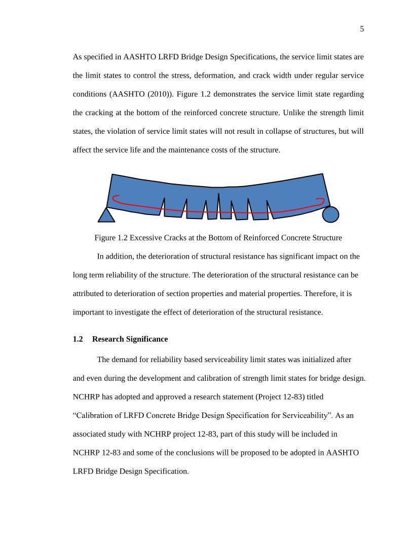
5
As specified in AASHTO LRFD Bridge Design Specifications, the service limit states are
the limit states to control the stress, deformation, and crack width under regular service
conditions (AASHTO (2010)). Figure 1.2 demonstrates the service limit state regarding
the cracking at the bottom of the reinforced concrete structure. Unlike the strength limit
states, the violation of service limit states will not result in collapse of structures, but will
affect the service life and the maintenance costs of the structure.
Figure 1.2 Excessive Cracks at the Bottom of Reinforced Concrete Structure
In addition, the deterioration of structural resistance has significant impact on the
long term reliability of the structure. The deterioration of the structural resistance can be
attributed to deterioration of section properties and material properties. Therefore, it is
important to investigate the effect of deterioration of the structural resistance.
1.2 Research Significance
The demand for reliability based serviceability limit states was initialized after
and even during the development and calibration of strength limit states for bridge design.
NCHRP has adopted and approved a research statement (Project 12-83) titled
“Calibration of LRFD Concrete Bridge Design Specification for Serviceability”. As an
associated study with NCHRP project 12-83, part of this study will be included in
NCHRP 12-83 and some of the conclusions will be proposed to be adopted in AASHTO
LRFD Bridge Design Specification.
6
Although exceedance of serviceability limits state in bridge structures might not
result in catastrophic consequences directly, frequent violation of serviceability limit
states would cause accumulated damages over period of time, which would induce
significant influences or reduction of structural performance, human experience,
durability of structure, and would also increase the cost of maintenance. Reliability based
serviceability limit states would provide a rational approach to evaluate the performance
of the structure at serviceability limit state. Furthermore, Calibration of serviceability
limit state would enable the design for various scenarios to achieve a target reliability
level consistently. In addition, deterioration of structural resistance is also an important
factor that would affect the performance of the structure at long term. Therefore,
incorporating the deterioration of structural resistance into structural reliability analysis
would provide a more insightful understanding of structural reliability long term.
1.3 Objectives and Scope
The primary objective of this research is to develop and calibrate various
serviceability limit states for concrete girder bridges using a reliability-based approach.
Based on the research, new design criteria or parameters such as new live load and
resistance factors or design provisions are proposed for various serviceability limit states.
In this research, databases for prestressed concrete girder bridges and reinforced
concrete decks were assembled. The comprehensive live load study was performed using
the WIM data collected over different states, and statistical parameters of live load effect
were summarized for regular truck load as well as permit vehicle load. The
characterization of truck load at long term was investigated based on 10 years of WIM
7
data collected in New Jersey. Also, the resistance of structure was derived for various
limit states and the statistical model was developed based on statistical information of
various random variables. Based on developed load and resistance models, the structural
reliability analysis was performed. Various design parameters such as live load and
resistance factors and various design provisions were modified until a consistent, rational
safety level was achieved for each serviceability limit state. Furthermore, the
deterioration models for structural resistances were developed for various serviceability
limit states. The reliability analysis was performed incorporating deterioration model and
the analysis results were compared with the ones without considering the deterioration of
the structure.
1.4 Organization of the Thesis
The thesis contains seven chapters. This chapter serves as an introduction of the
thesis outlining the problem statement and statement of objectives.
Chapter two presents a comprehensive literature review of various issues and
available research experiences in various related topics, including a brief introduction on
past and current design code methodologies and calibration procedures, serviceability
limit states in various design codes, techniques for structural reliability analysis, target
reliability index, statistics for various random variables, crack control reinforcement and
provisions regarding control of crack in AASHTO Specification, and concrete tension
stresses.
Chapter three provides the derivation of structural resistance for various
serviceability limit states and also provides the development of statistical models for
8
resistance and dead load. The resistance models developed in this chapter will be applied
in structural analysis in Chapter six.
Chapter four describes development of live load models for reliability analysis.
The techniques utilized for analyzing and processing WIM data were described. The live
load effects from various data sources were summarized and discussed. The
characterization of truck load at long term was investigated based on 10 years of WIM
data collected in New Jersey. Finally, the live load models were developed for both
regular truck load and permit vehicle load.
Chapter five presents the deterioration models for different bridge elements. The
deterioration of structural section properties as well as material properties was discussed.
The deterioration model for different bridge elements were developed for various
serviceability limit states.
Chapter six presents the results from structural reliability analysis and calibration
of various serviceability limit states. Based on reliability analysis and calibration results,
new design parameters or design provisions were proposed to be included in AASHTO
LRFD Design Specification. Furthermore, the reliability analysis results that were
incorporated with a deterioration model were discussed and compared with the results not
considering a deterioration model of the structural resistance.
Chapter seven contains the summary and conclusions of this thesis.
9
2 LITERATURE REVIEW
CHAPTER 2
LITERATURE REVIEW
2.1 Bridge Design Specifications
Over the decades, bridge engineers strived to improve the design of bridges by
updating the design specifications followed over different states. Load and Resistance
Factor Designed (LRFD) was introduced by AASHTO in 1994 (AASHTO 1994) to
replace the allowable stress method (ASD) and load factor design (LFD) given in the
AASHTO 1992 code (AASHTO 1992). As a product of code calibration performed
during NCHRP Project 12-33, the AASHTO LRFD Design Specification was developed
based on a rational reliability based approach. It is approved that more uniform
reliability level could be achieved by designing using AASHTO LRFD Design
Specification. In contrast, the previous AASHTO 1992 code has been continuously
updated during its more than fifty years of service and was proven to result in
inconsistencies in safety levels for different spans and bridge materials (Nowak 1995).
The present code methodology utilizes reliability theory to achieve uniform safety levels
for different materials and span lengths and considers statistical variability of various
parameters for both loads and resistance.

10
2.1.1 Allowable Stress Design (ASD)
The Allowable Stress Design (ASD) specification which was used before the
adoption of the AASHTO LRFD Specification was based on basic principles that the
resistance should be greater than the loads applied. The design requirements were
designated in a terms of a fraction of yield strength of the material, which was named as
allowable stress. However, although ASD design specification is efficient in many earlier
designs such as truss and arch structures, it was found that ASD is not appropriate in
many design scenarios such as dealing residual stresses for thin walled sections. Thus,
adjustments were added to ASD to compensate the residual stresses.
Furthermore, since ASD was based on yield stress of materials rather than stress
interactions, it does not consider different load combinations for different scenarios. Also
since ASD was developed based on steel material, it might not be appropriate for other
materials especially non-linear materials such as concrete in which properties vary with
the load and the time.
As practitioners realized the inherit complexity of material and applied loads,
along with the development of the reliability based approach, a new, reliability based
bridge design specification was required.
2.1.2 Load and Resistance Factor Design (LRFD)
A new, reliability based design specification, Load and Resistance Factor Design,
LRFD was adopted by AASHTO in 1994. In comparison with previous specification, the
LRFD approach incorporated the variability of loads into the design and provides similar
reliability levels for different designs. The LRFD design specification was developed

11
based on reliability analysis considering the uncertainties of loads and resistances. In the
reliability analysis, the structural performance was measured by probability of failure or
reliability index. Various materials, section types and span lengths were considered
during the development of LRFD. Eq. 2.1 shows a basic form of the LRFD design
equation (Nowak, 1995). In this equation, the resistance factor, φ, with a value less than
or equal to 1.0 is applied to the resistance, Q. on the other hand, the load factor, γ, is
applied to each load component. Both resistance factors and load factors were selected
and calibrated through reliability analysis in order to achieve uniform reliability level for
different designs.
n i iR Q Eq. 2.1
Where,
φ = resistance factor,
Rn = nominal (design) resistance,
γi = load factor for given load type, and
Qi = nominal (design) load component.
2.1.3 Eurocode
Eurocode is a set of specifications developed by European Committee for
Standardization for structural design of construction works in European Union. There are
ten sections which have been developed and published as of 2002 as listed below:
EN 1990 Eurocode 0: Basis of Structural Design
EN 1991 Eurocode 1: Actions on structures
EN 1992 Eurocode 2: Design of concrete structures

12
EN 1993 Eurocode 3: Design of steel structures
EN 1994 Eurocode 4: Design of composite steel and concrete structures
EN 1995 Eurocode 5: Design of timber structures
EN 1996 Eurocode 6: Design of masonry structures
EN 1997 Eurocode 7: Geotechnical design
EN 1998 Eurocode 8: Design of structures for earthquake resistance
EN 1999 Eurocode 9: Design of aluminum structures
The concept of design working life is adopted in the Eurocode. The design
working life is the period of time that a structure can be used for its intended design
purpose without major repair but with anticipated maintenance. The design working life
of various categories is summarized in Table 2.1.
Table 2.1 Design Working Lives (adapted from Table (2.1) – EN1990)
design working
life category
design working life
(years) examples
1 10 temporary structures
2 10 to 25 replaceable structural parts, e.g. gantry
girders, bearings
3 15 to 30 agricultural and similar structures
4 50 building structures and other common
structures
5 100 monumental building structures, bridges
and other civil engineering structures
Eurocode also considers three different levels of reliability, RC1, RC2, RC3 that
relate to strength and service limit states. These levels of reliability correspond to three
different levels of consequences classes, CC1, CC2 and CC3, as defined in Table 2.2.
Table 2.2 Eurocode Consequence Classes (adapted from Table (B1) – EN1990)

13
consequence
class
description related to consequences
reliability
class
CC1 low consequence for loss of human life; economic, social or
environmental consequences small or negligible
RC1
CC2 moderate consequence for loss of human life; economic,
social or environmental consequences considerable
RC2
CC3 serious consequences for loss of human life, or for
economic, social or environmental concerns
RC3
2.1.4 Canadian Code
Both ultimate limit states (ULS) and serviceability limit states (SLS) were
included in Canadian Highway Bridge Design Code (CHBDC), and earlier Ontario
Highway Bridge Design Code (OHBDC). The calibration of ULS in Canadian Code
followed a similar procedure as calibration of the strength limit states in the AASHTO
LRFD Bridge Design Specifications. Thus, the outcomes of calibration such as load and
resistance factors are also similar to ones that are used in AASHTO LRFD Bridge Design
Specification. Also similar to AASHTO LRFD Specification, the serviceability limit
states have not been calibrated using a reliability based approach.
2.1.5 ISO 2394 Document (General Principles on Reliability for Structures)
The International Organization for Standardization (ISO) has published a
document “ISO 2394 Document (General Principles on Reliability for Structures)” which
provides general principles for reliability evaluation and the verification for structures.
The general principles presented in this document are applicable to various types
of structures such as buildings, bridges, industrial structures, etc. In addition, the general
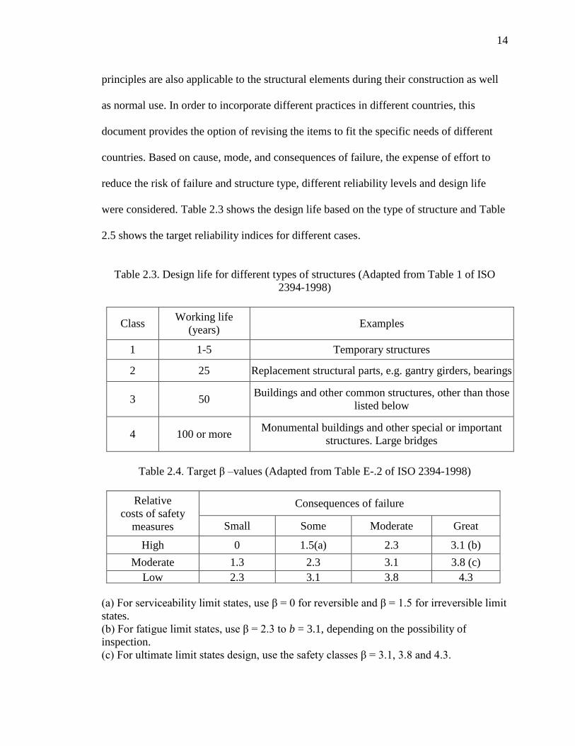
14
principles are also applicable to the structural elements during their construction as well
as normal use. In order to incorporate different practices in different countries, this
document provides the option of revising the items to fit the specific needs of different
countries. Based on cause, mode, and consequences of failure, the expense of effort to
reduce the risk of failure and structure type, different reliability levels and design life
were considered. Table 2.3 shows the design life based on the type of structure and Table
2.5 shows the target reliability indices for different cases.
Table 2.3. Design life for different types of structures (Adapted from Table 1 of ISO
2394-1998)
Class Working life
(years) Examples
1 1-5 Temporary structures
2 25 Replacement structural parts, e.g. gantry girders, bearings
3 50 Buildings and other common structures, other than those
listed below
4 100 or more Monumental buildings and other special or important
structures. Large bridges
Table 2.4. Target β –values (Adapted from Table E-.2 of ISO 2394-1998)
Relative
costs of safety
measures
Consequences of failure
Small Some Moderate Great
High 0 1.5(a) 2.3 3.1 (b)
Moderate 1.3 2.3 3.1 3.8 (c)
Low 2.3 3.1 3.8 4.3
(a) For serviceability limit states, use β = 0 for reversible and β = 1.5 for irreversible limit
states.
(b) For fatigue limit states, use β = 2.3 to b = 3.1, depending on the possibility of
inspection.
(c) For ultimate limit states design, use the safety classes β = 3.1, 3.8 and 4.3.

15
In addition, the table that shows the relationship between reliability index (β) and
probability of failure (Pf) as shown in Table 2.5 was included in the document.
Table 2.5. Relationship between β and Pf (Adapted from Table E.1 of ISO 2394-1998)
Pf 10-1 10-2 10-3 10-4 10-5 10-6 10-7
β 1.3 2.3 3.1 3.7 4.2 4.7 5.2
2.2 Serviceability Limit States
The limit state can be defined as a boundary between desired and undesired
performance (Nowak, 2000). If the limit state has been satisfied, the structure is safe. On
the other hand, if the limit state has been exceeded, the structure is “failed”. Considering
the corresponding consequences of the “failure”, the limit states can be categorized as
ultimate or strength limit state and serviceability limit state. The violation of ultimate
limit state causes the collapse of the structural member. Unlike the strength limit states,
the violation of service limit will affect the service life and the maintenance costs of the
structure.
In AASHTO LRFD Bridge Design Specifications, the service limit states refer to
the limit states that control the stress, deformation, and crack width under regular service
conditions (AASHTO (2010)). Similar to AASHTO, the cracking, deformation, stress,
and vibration serviceability limit states are considered in the Canadian Highway Bridge
Design Code (CAN/CSA-S6-06).
In European code, EN1990, and ISO 2394-1998, the serviceability limit state is
classified into two categories, irreversible and reversible serviceability limit states. In the

16
“designers’ handbook to Eurocode 1: basis of design” by Gulvanessian and Holicky,
1996. They defined reversible and irreversible service limit states as following:
a) Irreversible serviceability limit states (Figure 2.1-a), i.e. limit states that remain
permanently exceeded even when the actions that caused the infringement are
removed (e.g. a permanent local damage, permanent unacceptable deformations)
b) Reversible serviceability limit states (Figure 2.1-b), i.e. limit states that will not be
exceeded when the actions that caused the infringement are removed (e.g. cracks
of prestressed components, temporary deflections, excessive vibration).
Figure 2.1 irreversible (a) and reversible (b) limit states (Gulvanessian and Holicky, 1996)
2.3 Structural Reliability Analysis
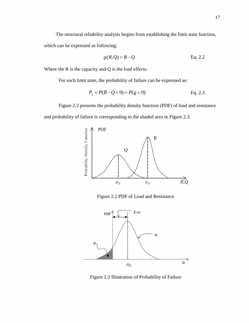
17
The structural reliability analysis begins from establishing the limit state function,
which can be expressed as following:
( , )g R Q R Q Eq. 2.2
Where the R is the capacity and Q is the load effects.
For each limit state, the probability of failure can be expressed as:
( 0) ( 0)fP P R Q P g Eq. 2.3
Figure 2.2 presents the probability density function (PDF) of load and resistance
and probability of failure is corresponding to the shaded area in Figure 2.3.
Figure 2.2 PDF of Load and Resistance
Figure 2.3 Illustration of Probability of Failure
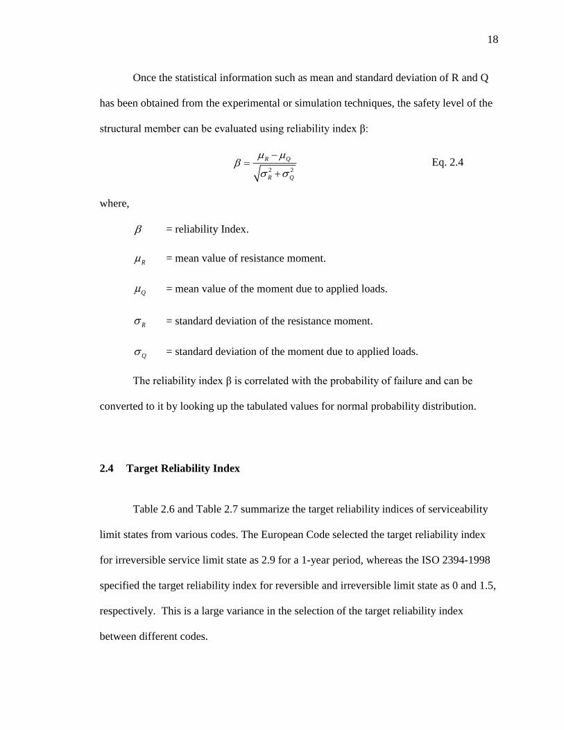
18
Once the statistical information such as mean and standard deviation of R and Q
has been obtained from the experimental or simulation techniques, the safety level of the
structural member can be evaluated using reliability index β:
2 2
R Q
R Q
Eq. 2.4
where,
= reliability Index.
R = mean value of resistance moment.
Q = mean value of the moment due to applied loads.
R = standard deviation of the resistance moment.
Q = standard deviation of the moment due to applied loads.
The reliability index β is correlated with the probability of failure and can be
converted to it by looking up the tabulated values for normal probability distribution.
2.4 Target Reliability Index
Table 2.6 and Table 2.7 summarize the target reliability indices of serviceability
limit states from various codes. The European Code selected the target reliability index
for irreversible service limit state as 2.9 for a 1-year period, whereas the ISO 2394-1998
specified the target reliability index for reversible and irreversible limit state as 0 and 1.5,
respectively. This is a large variance in the selection of the target reliability index
between different codes.

19
In this study, the preliminary target reliability indices were selected based on the
current practice and previous experiences from other Codes (European Code and ISO
2394 Document).
Table 2.6 Irreversible Service Limit States Reliability Indices (Adapted from Table (C2)-
EN1990)
Reliability Class Reference Period (years)
1 50
RC2 2.9 1.5
Table 2.7 Target Reliability Indices (Adapted from Table E-2 of ISO 2394-1998)
Relative Costs of
Safety Measures
Consequences of Failure
Small Some Moderate Great
High 0 1.5(a) 2.3 3.1 (b)
Moderate 1.3 2.3 3.1 3.8 (c)
Low 2.3 3.1 3.8 4.3
(a) For serviceability limit states, use β = 0 for reversible and β = 1.5 for irreversible limit
states.
(b) For fatigue limit states, use β = 2.3 to b = 3.1, depending on the possibility of
inspection.
(c) For ultimate limit states design, use the safety classes β = 3.1, 3.8 and 4.3.
2.5 Random Variables
In order to perform the reliability analysis for the serviceability limit states, the
probabilistic distribution and statistical parameters (μ and σ) of various random variables
needed to be collected or estimated. Table 2.8 shows a summary of the information based
on previous research studies by Siriaksorn and Naaman (1980) and Nowak (2008).

20
Table 2.8 Summary of typical statistical information for various variables from previous
research
Variables Distribution Mean, m COV., Ω Remarks
b , 1b , wb normal nb 0
h , 1fh , 2fh normal nh 1/6.4
pd , sd , 1e normal pnd , snd , 1ne 0.04-0.68/ nh
l , a normal nl , na 11/(32 )
cEC normal 33.6 0.1217 nominal=33
1.5
cc E c cE C f
rfC normal 9.374 0.0938
nominal=7.5 rf = rf
C
cf
cf lognormal 1.11 cnf 0.11
c normal cn = 150 0.03
cifC normal 0.6445 0.073 nominal=0.8 & cif = cif cC f
yf lognormal 1.13 ynf 0.03
sA normal 0.9 sA 0.015
sE normal snE 0.024
psA normal 1.01176 psnA 0.0125 psnA =0.153 2in
puf lognormal 1.03 punf 0.015 punf =270 ksi
pyf lognormal 1.027 pynf 0.022 pynf =240 ksi
psE normal 1.011 psnE 0.01 psnE =29000 ksi
sifC normal sinfC 0.08
sinfC =0.7
sif =sinf puC f
sefC normal senfC 0.08
senfC =0.83
sef =sef siC f
0 normal 0n 0.03

21
2.6 Crack Control Reinforcement
This section is a review of previous research studies, which focused on crack
control as well as predicting crack width in concrete members. Significant research has
been conducted to control cracks in concrete members resulting in the development of
numerous equations to predict the crack width at the bottom tension surface and the side
faces at the level of reinforcement. Equations available to predict crack width were
developed for concrete members with cover less than 2.5 in., but are not applicable for
beams with larger concrete covers. Various equations have been adopted by different
codes. However, for calibration purposes, there is a need to evaluate these equations with
regard to accuracy and applicability. The results from various equations will be
compared and validated using data collected from available literature.
2.6.1 Bottom Face of Concrete Member
One of the early studies by Clark (1956) included testing 58 specimens and
collecting over 105 crack width readings. Clark concluded that the average crack width
is closely related to the following parameters: 1) the diameter of the reinforcing bar, 2)
reinforcing bar area, 3) area of the beam section, and 4) the distance from the bottom
reinforcement to the beam bottom surface. Moreover, Clark stated that the average width
was also proportional to the stresses in the reinforcing bars beyond the cracking stress.
He suggested that the width of the cracks can be reduced by using a large number of
small diameter bars and by increasing the ratio of the steel reinforcement. Based on these
results, Equation 4 was developed to predict the average crack width of the concrete
beams. The maximum crack width was estimated by multiplying the average crack width
by 1.64 (Clark 1956).

22
1 2
1ave s
Dw C f C n
p p
Eq. 2.5
where,
avew = average width of cracks, in.
1C , 2C
= coefficients that depend on distribution of bond stress, bond
strength, and tensile strength of concrete, for Clark’s study;
8
1 2.27 10 /C h d d , 2 56.6C .
D = diameter of reinforcing bar, in.
p = /s eA A = cross-sectional area of reinforcement / cross-sectional area
of concrete.
eA = bd, in.²
sf = computed stress in reinforcement, psi.
n = ratio of modulus of elasticity of steel to concrete (assumed to be 8 in
Clark’s study)
h = overall depth of beam/slab, in.
d = distance from compressive face of beam/slab to centroid of
longitudinal tensile reinforcement.
Kaar and Mattock (1963) also developed a well-known crack width equation for
bottom face cracking:
40.115b sw f A Eq. 2.6
where,
bw
= maximum crack width, 0.001 in.

23
= ratio of distances to neutral axis from extreme tension fiber and from
centroid of reinforcement.
sf = steel stress calculated by elastic crack section theory, ksi.
cd
= bottom cover measured from center of lowest bar, in.
A = average effective concrete area around reinforcing bar, having same
centroid as reinforcement, in.²
Broms (1965) conducted tests on 37 tension and 10 flexural members to analyze
crack width and crack spacing. Broms observed that the crack spacing decreased rapidly
with increasing load and that a number of primary tensile cracks formed on the surface of
flexural and tension members. Secondary tensile cracks were confined to the
surrounding area of reinforcement. The study concluded that the absolute minimum
visible crack spacing is the same along the distance from the surface to the center of the
reinforcing bar located nearest to the surface of the member. Thus, the theoretical
minimum crack spacing is equal to the thickness of the concrete cover (Broms, 1965).
Gergely and Lutz (1968) developed an equation to predict the crack width based
on a detailed statistical assessment of experimental data available in the literature at the
time. Gergely and Lutz identified various parameters, such as reinforcing bar locations,
stresses in the reinforcement, concrete cover depth, and spacing of the reinforcement as
the controlling factors affecting the crack width. The Gergely and Lutz (1968) equation
is presented as follows:
30.076b s cw f Ad Eq. 2.7
where,

24
bw
= maximum crack width, 0.001 in.
= ratio of distances to neutral axis from extreme tension fiber and from
centroid of reinforcement.
sf = steel stress calculated by elastic crack section theory, ksi.
cd
= bottom cover measured from center of lowest bar, in.
A = average effective concrete area around reinforcing bar, having same
centroid as reinforcement, in.²
The maximum concrete cover tested in this study was 3.31 inches. However, only
three test specimens with cover greater than 2.5 in. were tested in the study.
In the study by Frosch (1999), the crack widths were determined from an equation
developed based on a physical model. Results were compared with the test data used in
Kaar and Mattock (1963) and Gergely and Lutz (1968). The crack width model
developed in this study showed that the crack spacing and width are functions of the
distance between the reinforcing steel. Crack control can be achieved by limiting the
spacing of these reinforcing bars. Based on the research findings, Frosch suggested that
limiting the maximum bar spacing would prevent large cracks in the concrete beams.
Based on the physical model, the equation to calculate the maximum crack width for
uncoated reinforcement was developed as shown below (Frosch 1999):
2
22
2
sc c
s
f sw d
E
Eq. 2.8
where,
s = maximum permissible bar spacing, in.

25
cw
= limiting crack width, in. (0.016 in, based on ACI 318-95).
sE
= elastic modulus of steel reinforcement (can be taken as 29000 ksi.)
= 1.0 + 0.08 cd
cd
= bottom cover measured from center of lowest bar, in.
sf = stress in steel reinforcement.
Frosch (1999) suggested that for epoxy-coated reinforcement, the above equation
should be multiplied by a factor of 2. The equation above is rearranged to solve for the
allowable bar spacing:
2
222
c sc
s
w Es d
f
Eq. 2.9
Based on the physical model, the following design recommendation was presented that
addressed the use of both the uncoated and coated reinforcement. The equation to
calculate the maximum spacing of reinforcement was given as follows (Frosch 1999) :
12 2 123
cs s
s
ds
Eq. 2.10
where,
cd = thickness of concrete cover measured from extreme tension fiber to center of
bar or wire located closest thereto, in.
s = maximum spacing of reinforcement, in.
36s c
sf

26
s = reinforcement factor
c = reinforcement coating factor: 1.0 for uncoated reinforcement; 0.5 for epoxy-
coated reinforcement, unless test data can justify a higher value.
sf = calculated stress in reinforcement at service load, ksi. It shall be computed as
the moment divided by the product of steel area and internal moment arm. It shall
be permitted to take sf as 60 percent of the specified yield strength yf .
Frosch (2001) summarized the physical model for cracking and illustrated the
development and limitations of the proposed design method. Based on the physical
model, he recommended formulas for calculating the maximum crack width for uncoated
and epoxy-coated reinforcement, as well as the design recommendation for their use
similar to those presented in Frosch (1999).
Epoxy-coated reinforcement is widely used to increase the durability of
structures. The epoxy-coated reinforcement has been shown to lessen bond strength that
can decrease crack spacing and bigger crack widths compared to uncoated reinforcement
(Blackmand and Frosch 2005). Blackman and Frosch investigated crack width of
concrete beams with epoxy-coated reinforcement. The primary variables used in the
study include epoxy coating thickness and reinforcing bar spacing. Blackman and Frosch
designed ten slab specimens in order to examine the effect of epoxy coating on cracks. It
was concluded that the epoxy coating thickness does not affect the concrete crack
significantly. Frosch (1999), Frosch (2001), Frosch (2002), and Blackman and Frosch
(2005) presented an equation to compare the average-measured crack spacing for the
uncoated and epoxy coated bars with the calculated values:

27
*
c sS d Eq. 2.11
where,
cS = crack spacing
*d = controlling cover distance
s = crack spacing factor: 1.0 for minimum crack spacing; 1.5 for average crack
spacing; 2.0 for maximum crack spacing
Choi and Oh (2009) studied the crack width for transversely post-tensioned
concrete deck slabs in box girder bridges. They tested four full-scale concrete box girder
segments and then derived the maximum crack width equation from the testing data:
,6
max 03 10 0.75t eff
s s
st pt
A h xw f f
A A d x
Eq. 2.12
1
=ap s
as p
n
n
Eq. 2.13
where,
maxw = predicted maximum crack width in mm
stA = total area of reinforcing bars
ptA = total area of prestressing tendons
x = depth of neutral axis in mm
h = height of cross section
d = effective depth in mm

28
sf = increment of reinforcing bar stress after decompression
0f = steel stress at the initial occurrence of crack
s = diameter of reinforcing bar in mm
p = diameter of prestressing tendons
ap
as
= 0.465 for grouted post-tensioned tendons
Cracking of structures is rather common and is not always damaging to the
structure. However, when considering a bridge deck, moderately sized cracking can be
detrimental to the longevity of the structure due to the exposure to harsh environments.
Recently, thicker concrete covers, coupled with the use of high-performance concrete, are
becoming increasingly popular because of their durability. This often results in
unrealistic bar spacing and prevents the use of contemporary crack control practices that
are based on statistical studies. Therefore, it is desirable to develop methods to predict
average and maximum crack widths of reinforced concrete members with thicker
concrete covers at various locations.
2.6.2 Side Face of Concrete Member
In general, large cracks are expected only at the extreme tensile face of the beam.
However, Beeby (1979) conducted studies that showed the largest crack widths occurring
in the web along the beam side face with the maximum widths occurring at about mid-
height.
Frantz and Breen (1980a) observed very wide cracks near mid-depth on the side
faces of several 8-ft deep inverted T beams. Although the crack width at the flexural

29
reinforcement level was acceptable, the maximum crack width on the side face were up
to three times as wide as the crack width at the flexural reinforcement level. The authors
tested 44 laboratory size specimens to investigate the factors affects side face cracking:
skin reinforcement cover, web width, area and distribution of skin reinforcement, and
depth of beam. They concluded the following based on the testing results:
1. Since the skin reinforcement is only effective in a narrow strip of concrete along
each side face, the web width has no significant effect on the web crack width.
2. The skin reinforcement cover did not affect the web crack width. However, the
effectiveness of the skin reinforcement in controlling the web crack widths
decreased as the skin reinforcement cover increased.
3. The skin reinforcement should be located within 5/8 of the tension zone closest to
the main reinforcement.
4. The effectiveness of skin reinforcement can be related to the skin reinforcement
ratio, which is the area of skin reinforcement divided by the area of concrete strips
along the side faces affected by the reinforcement.
5. The side face crack width increased as the beam tension depth increased.
Frantz and Breen (1980b) proposed the following design recommendations of
skin reinforcement for large reinforced concrete beams:
1. For more than 36 in. deep concrete member, the longitudinal skin reinforcement
shall be distributed uniformly over ½ of the depth nearest the main reinforcement
along the side faces.
30
2. The skin reinforcement ratio Q, which is the ratio of total area of skin
reinforcement to the total area of strips along each side face, should be designed
according to the following provisions:
a. If 36 . 100 .in d in , 0.00024 30Q d
b. If 100 .d in , 0.011 0.00058Q d
3. The maximum spacing of skin reinforcement shall be limited to smaller of d/10 or
12 in.
Adebar and Leeuwen (1999) conducted an experimental study to investigate the
appropriate amount of distribution of the skin reinforcement in controlling flexural and
diagonal cracking. The authors tested 21 large concrete beams having web depth equal to
47 inch. The area of skin reinforcement was varied from 50 to 300 percent of the ACI
Code and AASHTO Specification requirements. Based on the testing results, they
reached the following conclusions:
1. The web crack width decreased as the amount of well-distributed skin
reinforcement increased.
2. The application of welded wire fabric reduced the crack width due to the smaller
diameter and more closely spacing.
3. The maximum diagonal crack width in the webs of large beams depends on the
following parameters:
a. The magnitude of shear stress
b. The longitudinal strain of the longitudinal reinforcement on the flexural
tension side
c. The amount and arrangement of transverse reinforcement
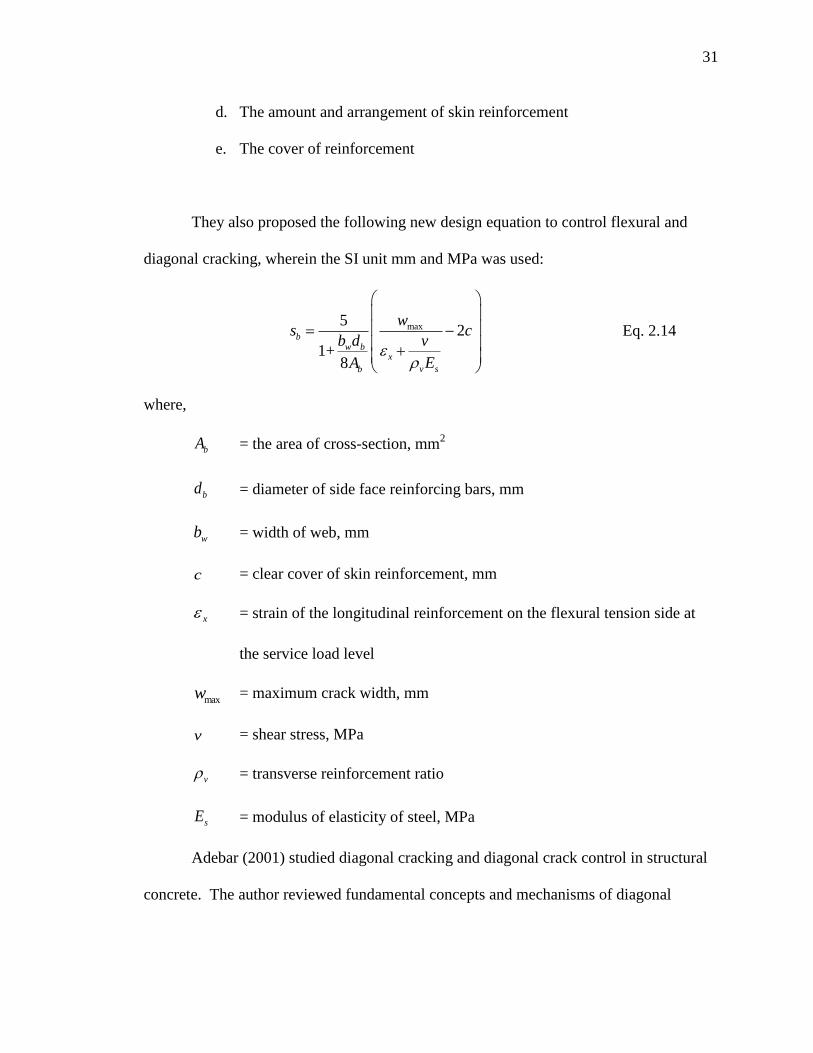
31
d. The amount and arrangement of skin reinforcement
e. The cover of reinforcement
They also proposed the following new design equation to control flexural and
diagonal cracking, wherein the SI unit mm and MPa was used:
max52
1+8
bw b
x
v sb
ws c
b d v
EA
Eq. 2.14
where,
bA = the area of cross-section, mm2
bd = diameter of side face reinforcing bars, mm
wb = width of web, mm
c = clear cover of skin reinforcement, mm
x = strain of the longitudinal reinforcement on the flexural tension side at
the service load level
maxw = maximum crack width, mm
v = shear stress, MPa
v = transverse reinforcement ratio
sE = modulus of elasticity of steel, MPa
Adebar (2001) studied diagonal cracking and diagonal crack control in structural
concrete. The author reviewed fundamental concepts and mechanisms of diagonal

32
cracking. Additionally, the author proposed the same equation as Eq. (3.2-10) for
diagonal cracking control.
Frosch (2002) conducted research on the modeling and control of cracking in side
face of the concrete beams. The study showed that the maximum skin reinforcement
spacing is a function of the concrete cover from the skin reinforcement. It was also
shown that a maximum bar spacing of 12 in. provides reasonable crack control up to 3 in.
of concrete cover. The crack model developed by Frosch allows for the calculation of the
crack width at any point along the cross section. A profile of the crack width through the
depth of the section is more easily created, allowing for information regarding optimum
locations for placing skin reinforcement for the purpose of controlling side face cracks.
Frosch (2002) showed that the crack spacing and crack width along the side face are
functions of the distance from the reinforcement, so the crack can be controlled by adding
skin reinforcement and limiting the reinforcement spacing. Since the maximum crack
width was observed at halfway between the reinforcement and neutral axis, the following
equation can be used to solve for the crack width at / 2x d c :
2
2 1
2c s sw d d c
Eq. 2.15
where,
s = reinforcing strain = /s sf E
sd = skin reinforcement cover, in.
d = effective depth, in.
c = depth of neutral axis, in.

33
The study of the physical model showed that sections with effective depth of 36
in. and covers up to 3 in. can be designed without skin reinforcement. For thicker covers,
the maximum effective depth not requiring skin reinforcement should be decreased.
Moreover, there is a reduction in the maximum effective depth for covers thicker than 3
in. for Grade 60 reinforcement resulting in a maximum depth, d = 36 inches.
In order to prevent excessive cracks throughout the depth of the section, maximum
spacing of the reinforcement should be determined. According to Frosch (2002), the
placement of the first bar is the most critical for the spacing of the skin reinforcement.
The maximum crack width was calculated halfway between the primary reinforcement
and the first skin reinforcement at a distance /2x s , yielding the following equation:
2
222
ss s
s
f sw d
E
Eq. 2.16
For sections where skin reinforcement exists, it is necessary to determine the location in
the section where the reinforcement can be discontinued. Since crack widths are
controlled by skin reinforcement below its end point, it is required to calculate the
maximum distance sna where the skin reinforcement can be eliminated. The maximum
crack width will occur approximately halfway between the neutral axis and the location
of the first layer of skin reinforcement at a distance / 2nax s from the neutral axis. The
maximum crack width can be calculated with the following equation based on the
physical model developed by Frosch (2002):
2
2
2
s nas na s
sw s d
d c
Eq. 2.17

34
where,
nas = maximum distance where the skin reinforcement can be eliminated.
Frosch recommended that the design formula should be based on a physical model to
address the control of cracking in reinforced concrete structures and to unify the design
criteria for controlling cracking in side and bottom faces. Frosch (2002) recommended
the maximum spacing of flexural tension reinforcement as follows:
12 2 123
cs s
s
ds
Eq. 2.18
where,
36s
sf
= thickness of concrete cover, in., for bottom-face reinforcement,
measured from extreme tension fiber to center of bar, and for skin
reinforcement, measured from side face to center of bar
S = maximum spacing of reinforcement, in.
s = reinforcement factor
sf = Calculated stress in reinforcement at service load, ksi. It shall be
computed as the moment divided by the product of steel area and
internal moment arm. It shall be permitted to take sf as 60 percent of
the specified yield strength yf

35
Skin reinforcement shall be required along both side faces of a member for a
distance d/2 from the nearest flexural tension reinforcement if the effective depth exceeds
the depth calculated by equation shown below:
42 2 36s c sd d Eq. 2.19
2.6.3 Summary
Section 3.2 presented a review of previous research work related to crack control
of the bottom face and side face of concrete members. Researchers attempted to develop
more accurate equations to predict the maximum crack width, and then control the crack
width by distributing the reinforcement in an appropriate way.
Furthermore, various crack width prediction equations were validated with test
data collected from literature. Frosch (1999) equation will be checked further since it
provided good correlation with test data, and is considered the basis of the AASHTO
LRFD (2008) provisions. Moreover, Response 2000 computer program and Frosch
(1999) were validated and calibrated using the test data from previous studies. The
results indicated that the calibrated Response 2000 provided good correlation with test
data. Therefore, the research team will validate the calibrated Response 2000 further
with data from various beam sections including deep members.
2.7 Control of Cracks in Current AASHTO LRFD Specifications Provisions
Section 2.6 presented a summary of the research on the maximum crack width
and crack control. This section provides a review of code provisions related to the
distribution of crack control reinforcement.
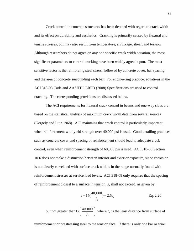
36
Crack control in concrete structures has been debated with regard to crack width
and its effect on durability and aesthetics. Cracking is primarily caused by flexural and
tensile stresses, but may also result from temperature, shrinkage, shear, and torsion.
Although researchers do not agree on any one specific crack width equation, the most
significant parameters to control cracking have been widely agreed upon. The most
sensitive factor is the reinforcing steel stress, followed by concrete cover, bar spacing,
and the area of concrete surrounding each bar. For engineering practice, equations in the
ACI 318-08 Code and AASHTO LRFD (2008) Specifications are used to control
cracking. The corresponding provisions are discussed below.
The ACI requirements for flexural crack control in beams and one-way slabs are
based on the statistical analysis of maximum crack width data from several sources
(Gergely and Lutz 1968). ACI maintains that crack control is particularly important
when reinforcement with yield strength over 40,000 psi is used. Good detailing practices
such as concrete cover and spacing of reinforcement should lead to adequate crack
control, even when reinforcement strength of 60,000 psi is used. ACI 318-08 Section
10.6 does not make a distinction between interior and exterior exposure, since corrosion
is not clearly correlated with surface crack widths in the range normally found with
reinforcement stresses at service load levels. ACI 318-08 only requires that the spacing
of reinforcement closest to a surface in tension, s, shall not exceed, as given by:
40,000
15( ) 2.5 c
s
s cf
Eq. 2.20
but not greater than40,000
12sf
, where cc is the least distance from surface of
reinforcement or prestressing steel to the tension face. If there is only one bar or wire
37
nearest to the extreme tension face s used in Eq. (3.3-1) becomes the width of the extreme
tension face. These provisions are not sufficient for structures subject to very aggressive
exposure or designed to be watertight. Special investigation is required for structures
subject to very aggressive exposure or designed to be watertight. ACI 318-08
recommends the use of several bars at moderate spacing rather than fewer bars at larger
spacing to control cracking. These provisions were updated recently to reflect the higher
service stresses that occur in flexural reinforcement with the use of the load combinations
introduced in ACI 318-02. The maximum bar spacing is specified to directly control
cracking. Similar recommendations have been stated for deep beams with the
requirement of skin reinforcement.
AASHTO LRFD (2008) also provides provisions for reinforcement spacing to
control flexural cracking. Similar to the equation adopted in ACI, AASHTO emphasizes
the importance of reinforcement detailing and the notion that smaller bars at moderate
spacing are more effective than larger bars of equivalent area. AASHTO also agrees with
ACI 318-08 on most of the important parameters affecting crack width and specifies a
formula for distribution of reinforcement to control cracking. The equation in AASHTO
LRFD (2008) is based on the physical crack model of Frosch (2001) rather than on the
statistically-based model used in previous editions. The equation limits bar spacing
rather than crack width as follows:
700
2ec
s ss
s df
Eq. 2.21
where,

38
s = 10.7( )
c
c
d
h d
(geometric relationship between crack width at tension
face versus crack width at reinforcement level)
e = exposure factor = 1.00 for Class I exposure, 0.75 for Class II exposure
cd
= thickness of concrete cover measured from extreme tension fiber to
center of the flexural reinforcement located closest thereto (in.)
ssf
= tensile stress in steel reinforcement at the service limit state (ksi)
h = overall thickness of depth of the component (in.)
Unlike ACI, AASHTO specifies exposure conditions to meet the needs of the
authority having jurisdiction. Class I exposure condition is based on a crack width of
0.017 in. and applies when cracks can be tolerated due to reduced concerns of appearance
and/or corrosion. This exposure class can be thought of as an upper bound in regards to
crack width for appearance and corrosion. Class II exposure condition applies to
transverse design of segmental concrete box girders for any loads applied prior to
attaining full nominal concrete strength. This is used when there is an increased concern
of appearance and/or corrosion such as in substructures exposed to water and decks.
AASHTO LRFD also specifies requirements for skin reinforcement based on ACI 318-
02. The AASHTO Equation (or Eq. 20 shown above) also applies to both reinforced and
prestressed concrete with specifications on the steel stresses used. In general, if
AASHTO Class II exposure condition is used, all AASHTO spacings were less than
those derived by the ACI equation. However, if Class I exposure condition is used, ACI
spacing becomes more conservative.

39
2.8 Concrete Tension Stresses
The overall objective of this literature review is to look into the origins of the
allowable tensile stress limits in the current design provisions. The review traces back to
the original and the subsequent changes and the research of the tensile strength limit
conducted by various researchers.
This literature review is organized in three sections. The first section is the
historical development of tensile strength limit provisions in the design specifications.
The second section discusses the previous research of tensile strength limit, while the last
section presents the summary of the previous research especially concerning the variation
of the tensile stress limit.
2.8.1 Historical Development of Tensile Strength Limit Provisions
The early discussion of cracking control is diverse. At the First United States
Conference on Prestressed Concrete in 1951, some experts believed the completely
crackless concrete member is only better for a specific purpose, but other experts thought
the cracking of prestressed concrete beam is of the same importance as the yielding. In
1958, the “Tentative Recommendations for Prestressed Concrete” proposed by ACI-
ASCE Committee 323 (ACI-ASCE 323) suggested that the prestressed concrete stresses
before losses due to creep and shrinkage should adhere to the following limits ( please
note the unit in the following provisions is psi for the allowable tensile stress):
1. 3 cif for members without non-prestressed reinforcement;
2. 6 cif for members with non-prestressed reinforcement provided to resist the
tensile force in concrete; computed on the basis of an uncracked section.

40
The Building Code Requirements for Reinforced Concrete (ACI 318-63) included
the recommendation for the tensile stress limits as proposed by joint committee ACI-
ASCE 323, with some modifications, as follows:
1. 3 cif for members without auxiliary reinforcement in the tension zone;
2. When the calculated tension stress exceeds 3 cif , reinforcement shall be
provided to resist the total tension force in the concrete computed on the
assumption of uncracked section.
The Building Code Requirements for Reinforced Concrete (ACI 318-77)
modified the allowable tensile stress limit as follows:
1. 6 cif for the extreme fiber stress in tension at ends of simply supported
members;
2. 3 cif for the extreme fiber stress in tension at other locations.
ACI 318-08, Section 18.4.1 specifies the allowable tensile in concrete
immediately after prestress transfer (before time-dependent prestress losses) as follows:
1. Where computed concrete tensile strength, tf , exceeds 6 cif at ends of simply
supported members, or 3 cif at other locations, additional bonded reinforcement
shall be provided in the tensile zone to resist the total tensile force in concrete
computed with the assumption of an uncracked section.

41
Table 2.9- Tensile Stress Limits in Prestressed Concrete at Service Limit State After
Losses, Fully Prestressed Components (AASHTO 2008 Table 5.9.4.2.2-1)
Bridge
Type Location Stress Limit
Other Than
Segmentally
Constructed
Bridges
Tension in the precompressed Tensile Zone Bridges,
Assuming Uncracked Sections
For components with bonded prestressing tendons
or reinforcement that are subjected to not worse
than moderate corrosion condition.
For components with bonded prestressing tendons
or reinforcement that are subjected to severe
corrosive conditions
For components with unbounded prestressing
tendons
0.19 ( )cf ksi
0.0948 ( )cf ksi
No tension
Segmentally
Constructed
Bridges
Longitudinal Stresses Through Joints in the
Precompressed Tensile Zone
Joints with minimum bonded auxiliary
reinforcement through the joints sufficient to
carry the calculated longitudinal tensile force at a
stress of 0.5 fy; internal tendons or external
tendons
Joints without the minimum bonded auxiliary
reinforcement through joints
0.0948 ( )cf ksi
No tension
Transverse Stress Through Joints
Tension in the transverse direction in precompressed
tensile zone
0.0948 ( )cf ksi
Principal Tensile Stress at Neutral Axis in Web
All types of segmental concrete bridges with internal
and/or external tendons, unless the Owner imposes
other criteria for critical structures.
0.110 ( )cf ksi
The AASHTO Standard Specifications for Highway Bridges (AASHTO 1992)
specified the allowable tensile stresses, before losses due to creep and shrinkage, as
follows:
1. 200 psi or 3 cif for members in tension areas with no bonded reinforcement;
42
2. Where the calculated tensile exceeds this value, reinforcement shall be provided
to resist the total tension force in the concrete computed on the assumption of
uncracked section. The maximum tensile stress shall not exceed 7.5 cif .
Table 2.9 shows the tensile stress limits and provisions by the AASHTO LRFD
(2008) Specification. It is noted that the only change from the AASHTO LRFD (2004)
Specifications is the principal tensile stress at Neutral Axis in Web.
2.8.2 Research Related to the Tensile Stress Limits
The majority of the research performed on tensile strength of concrete attempted
to develop more precise prediction equations for the tensile strength. However, with the
introduction of HPC and other pozzolanic material such as silica fume, fly ash, and slag,
and based on their limited test results, few researchers aimed to revise the allowable
tensile stress limits. Literature was reviewed to include the background work in this area
that would either support such revisions or retain the current limits in the AASHTO
LRFD (2008) provisions during the code calibration process.
McNeely and Lash (1963) performed tests on 35 cylinders to evaluate the
compressive and tensile strengths and to evaluate the effect of pre-compression, loading
rate, and cold temperature on the modulus of rupture. The results indicated that pre-
compression had no significant effect on the tensile strength, and that the tensile strength
is greater at zero oF than at room temperature. Based on their test data, they also
concluded that the average tensile strength was 455 psi with a standard deviation of 30
psi.

43
Carrasquillo et al. (1981) performed uniaxial compressive tests on 4 × 8 in. and 6
× 12 in. concrete cylinders and modulus of rupture tests on 4 × 4 × 14 in. beams. They
used Type I Portland cement with water-cement ratio between 0.32 and 0.70. The
uniaxial compressive testing results ranged from 3000 to 11,000 psi. Based on their test
results, they recommended 11.7 cf psi for the modulus of rupture and 6.8 cf psi for
the splitting tensile strength. They also reported that drying has more effect on the high
strength concrete than normal strength concrete.
Carino and Lew (1982) derived an expression for the tensile splitting strength as a
function of the compressive strength of normal weight concrete. They analyzed data
from the published literature as well as the data acquired from the National Bureau of
Standards (NBS) to formulate a more appropriate equation. They compared various
forms of equations based on regression analysis of the NBS data, and concluded that an
equation with a power function provides the best correlation with experimental data as
follows:
0.730.80( )ct cf f , psi
Eq. 2.22
Raphael (1984) studied the relationship between the tensile and the compressive
strength based on 12,000 tests compiled from Gonnerman and Shuman (1928), Walker
and Bloem (1960), Grieb and Werner (1962), and Houk (1965). Figure 2.4 illustrates the
compiled data with best-fit equations. They suggested that the modulus of rupture can be
predicted using 2' 32.3 cf (in psi) and is more suitable for concrete compressive strengths
of up to 9,000 psi (Figure 2.4).
44
Oluokun et. al (1991) carried out tests on specimens from different mixes to
establish a relationship between splitting tensile and compressive strengths at early ages.
The tests were performed at the ages of 6 and 12 hr and 1, 2, 3, 7, and 28 days. They
performed regression analysis and validated the results with the testing data from several
different references. They proposed two equations for 1000cf psi and 1000cf psi ,
respectively.
0.790.584( )ct cf f , psi, for 1000cf psi Eq. 2.23
0.60.928( )ct cf f , psi, for 1000cf psi Eq. 2.24
Huo and Tadros (2000) studied the allowable tensile stress of high performance
concrete (HPC) bridge beams. The authors recommended that, if high performance
concrete is used in bridge beams, the allowable tensile stress should be increased from
7.5 cf to 10 cf , in psi, (0.62 cf to 0.83 cf MPa) at release and from 6.0 cf to 7.9
cf , in psi, (0.50 cf to 0.66 cf (in MPa)) at service. The actual test results of the
Texas HPC mixes showed that the new allowable stress limits were adequate and
reasonable.
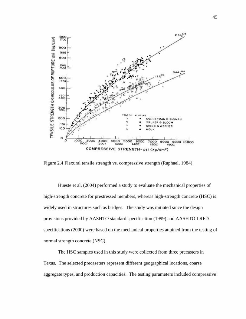
45
Figure 2.4 Flexural tensile strength vs. compressive strength (Raphael, 1984)
Hueste et al. (2004) performed a study to evaluate the mechanical properties of
high-strength concrete for prestressed members, whereas high-strength concrete (HSC) is
widely used in structures such as bridges. The study was initiated since the design
provisions provided by AASHTO standard specification (1999) and AASHTO LRFD
specifications (2000) were based on the mechanical properties attained from the testing of
normal strength concrete (NSC).
The HSC samples used in this study were collected from three precasters in
Texas. The selected precaseters represent different geographical locations, coarse
aggregate types, and production capacities. The testing parameters included compressive
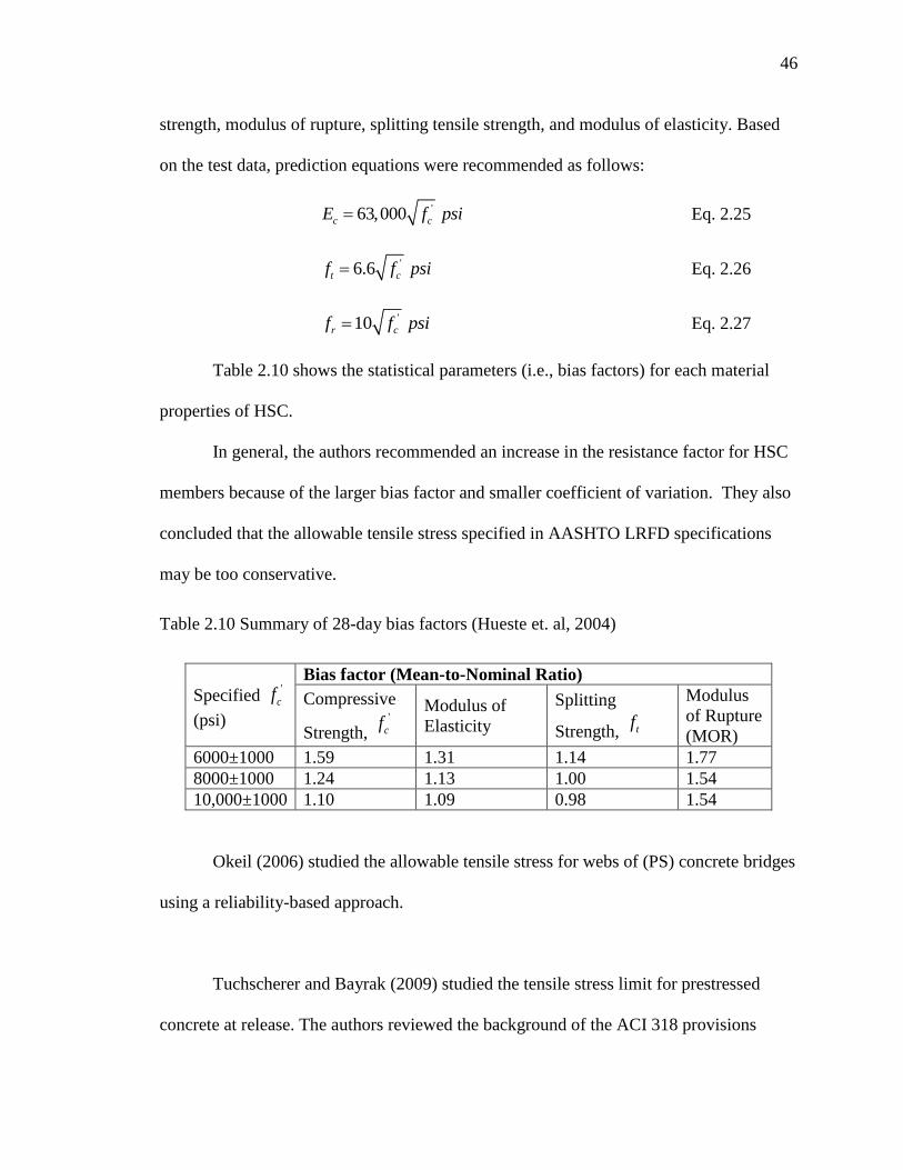
46
strength, modulus of rupture, splitting tensile strength, and modulus of elasticity. Based
on the test data, prediction equations were recommended as follows:
'63,000c cE f psi Eq. 2.25
'6.6t cf f psi Eq. 2.26
'10r cf f psi Eq. 2.27
Table 2.10 shows the statistical parameters (i.e., bias factors) for each material
properties of HSC.
In general, the authors recommended an increase in the resistance factor for HSC
members because of the larger bias factor and smaller coefficient of variation. They also
concluded that the allowable tensile stress specified in AASHTO LRFD specifications
may be too conservative.
Table 2.10 Summary of 28-day bias factors (Hueste et. al, 2004)
Specified '
cf
(psi)
Bias factor (Mean-to-Nominal Ratio)
Compressive
Strength, '
cf Modulus of
Elasticity
Splitting
Strength, tf
Modulus
of Rupture
(MOR)
6000±1000 1.59 1.31 1.14 1.77
8000±1000 1.24 1.13 1.00 1.54
10,000±1000 1.10 1.09 0.98 1.54
Okeil (2006) studied the allowable tensile stress for webs of (PS) concrete bridges
using a reliability-based approach.
Tuchscherer and Bayrak (2009) studied the tensile stress limit for prestressed
concrete at release. The authors reviewed the background of the ACI 318 provisions

47
about the allowable tensile stress limit for prestressed concrete. The allowable tensile
stress for prestressed concrete was 3 cf , in psi, until 1977. After 1977, the ACI Code
changed the limit to 6 cf , in psi. For the tensile stress at the ends of simply supported
members, the author questioned this change of the allowable tensile stress and performed
the experimental work for seven 54 in. deep bridge beam. The results suggest that for
some deep girders, the current ACI provisions about the allowable tensile stress limit is
not adequate to prevent cracking at prestress release, so the author recommended the
allowable tensile stress should be changed from 6 cf psi to 4 cf
, in psi.
Various authors studied the effects of various types of aggregates and other
materials on the tensile strength of concrete. Lam et al. (1998) studied the effect of fly
ash and silica fume on the compressive and tensile strength of concrete. They have tested
24 mixes with various water-cementitious material ratios, and various percentages of fly
ash and Silica fume. Results show that the splitting tensile strength increased 13% when
adding 5% silica fume.
Haque and Kayali (1998) studied the properties of high-strength concrete using
fine fly ash. They concluded that the indirect tensile strength was about 5 and 6% of their
respective compressive strength.
Zain et. al (2002) attempted to find a new expression for the tensile strength of
HPC arguing that the current ACI prediction equation is too simple to cover HPC at
different ages. Their new equation was related to the compressive strength of concrete,
W/B ratio, and concrete age. The equation was based on experimental data and linear
regression technique, as follows:

48
0.10 7.11
cct
c
ff
f
, MPa Eq. 2.28
Similar analysis was performed with regard to the relationship between the tensile
strength and the W/B ratio and concrete age, as shown in Eq. (3.7.2-8) and (3.7.2-9),
respectively.
0.070.54 ( / )ct cf f W B ,MPa Eq. 2.29
0.04
, ,
28
0.59 ( )ct t c t
tf f
t , MPa Eq. 2.30
where ,ct tf = the splitting tensile strength (MPa), at age t = in days, ,c tf = the
compressive strength (in MPA) at age t = days, and t is age of concrete in days.
Choi and Yuan (2005) studied the relationship between the splitting tensile
strength and compressive strength of Glass Fiber Reinforced Concrete (GFRC) and
Polypropylene Fiber Reinforced Concrete (PFRC) using experimental data. They
performed 5 mixes: 1) no fiber, 2) 1.0%, 3) 1.5% of glass fiber, 4) 1.0%, and 5) 1.5% of
polypropylene fiber. They have developed equations similar to the format used in the
ACI-318-08 Code in the SI system of units:
0.60ct cf f , For GFRC, MPa Eq. 2.31
0.55ct cf f , For PFRC, MPa Eq. 2.32
Bhanja and Sengupta (2005) studied the influence of silica fume on the tensile
strength by testing 30 mixes. The mixes have different W/B ratio and percentage of
Silica Fume. The compressive strength of concrete was measured, however, the splitting
tensile strength was estimated from the compressive strength by using empirical
correlation equations. They used regression analysis to obtain the relationship between
49
the 28-day splitting tensile strength and compressive strength, as shown in Equation
below
0.7170.284 ( )ct cf f , MPa Eq. 2.33
The authors also obtained the relationship between the 28-day flexural tensile
strength and compressive strength as shown in Equation below:
0.810.275 ( )ctf cf f , MPa Eq. 2.34
2.8.3 Summary
Most researchers attempted to develop more precise prediction equations for the
allowable tensile stress using the relationship between the tensile stress and compressive
strength. However, few researchers attempted to find the variation of allowable tensile
stress because of the application of new types of concrete such as High-Performance
concrete (HPC) and High-Strength Concrete (HSC). For example, as stated earlier, Huo
and Tadros (2000) studied the allowable tensile stress of HPC bridge girders and
advocated an increase in the allowable tensile stress from 7.5 cf to 10 cf psi (0.62
cf (to 0.83 cf MPa) at release and from 6.0 cf to 7.9 cf psi (0.50 cf to 0.66 cf
MPa) at service. In support of their recommendation, the authors show that the actual
test results from the Texas HPC mixes showed that the proposed new allowable stress
limits were adequate and reasonable. On the other hand, Tuchscherer and Bayrak (2009)
found out that the ACI allowable tensile stress limit of 6 cf psi at the end of prestressed
concrete beam is not adequate to prevent cracking and recommended that the allowable
50
tensile stress should be changed from 6 cf to 4 cf , in psi. This confirms the limit set
by AASHTO LRFD (2008) provisions at 3 cf , in psi.
2.9 Deflection of Concrete Members
The American Association of State Highway Transportation Officials (AASHTO)
Load and Resistance Factor Design (LRFD) Bridge Specification (2008) establishes the
use of a deflection design as optional criteria. Certain State Highway Agencies specify
their own deflection limits as a mandatory requirement. The deflection criteria in
AASHTO LRFD (2008) are shown as follows:
1. For the bridge designed for general vehicular load, the deflection
limitation is L/800;
2. For the bridge designed for vehicular and/or pedestrian loads, the
deflection limitation is L/1000;
3. For the bridge designed for vehicular load on cantilever arms, the
deflection limitation is L/300;
4. For the bridge designed for vehicular and/or pedestrian loads on
cantilever arms, the deflection limitation is L/375.
It is perceived that these deflection limits are usually based on a rather arbitrary
and sometimes conservative approach in designing bridges (Demitz et. al, 2003). This
raises questions on the rationality of these deflection limits in that pursuing a
conservative design approach does not take advantage of today’s bridge construction
technologies. In principle, the deflection limits were established to eliminate damage to
51
any structural and non-structural components due to excessive deformations as well as to
avoid loss of aesthetic appearance and interruption of its functionality. For highway
bridges, vehicle rideability and human responses to bridge vibration under normal traffic
conditions play an important role in determining the deflection limits. Moreover, if it is
believed that deflection limits should be specified as a design parameter, there is a need
for a rational approach to establish a limit state design philosophy that all designers can
justifiably use. If the deformation (deflection) requirements in AASHTO LRFD Bridge
Design Specifications, Subsection 2.5.2.6 become the controlling design issue, the most
economical bridge designs, based on ultimate strength criteria, cannot be achieved. Table
2.5.2.6.3-1 Traditional Minimum Depths for Constant Depth Superstructures in
AASHTO LRFD Bridge Design Specifications (2008) (shown in Table 2.11) will need to
be modified to reflect current bridge design use of high strength concrete (HSC). This
will enhance the use of HSC and address the bridge component property aspect. This
will offset the use of a deflection limitation; such as, L/800.
It is generally agreed that the deformation requirements (i.e. deflection limits and
corresponding span-to-depth ratio limits) were established to (a) prevent structural
damage due to excessive deflections, and (b) control of bridge vibrations to offset human
perceptions. The research team will provide a calibration procedure for deflection limit
state based on the currently specified AASHTO’s deflection limit at L/800. The
procedure will establish the calibrated live load factors for the Service I limit State.
However, it should be emphasized herein that the specifying deflection limits may
provide enough stiffness of bridge superstructure, but dynamic characteristics of a bridge
are determined by both mass and stiffness distributions of a bridge system. It is the

52
“resonances” due to the close frequencies of the bridge and truck loading system that
generate undesirable bridge vibration. For example, if the truck frequency is normally
between 2 and 5 Hz and if the bridge has a natural frequency around 2 Hz, there can be
excessive deflection and vibrations. In other words, the deflection limits by themselves
cannot provide an effective control of bridge vibration under normal traffic conditions.
A preliminary literature search indicated that the origin of the deformation
requirements in bridge designs may be traced back to 1871 with a set of specifications
established by the Phoenix Bridge Company (PBC). The ASCE report on deflection
limits of bridges (ASCE, 1958) has been widely cited for the evolution of these
requirements, (summarized in Table 2.12 below). The following conclusions may be
drawn from the ASCE report:
1. The deflection limits were established before the span-to-depth
ratio limits; that is, the span-to-depth ratio limits were used as indirect measures
of the deflection limits.
2. Both deflection and span-to-depth ratio limits were empirically
derived, mainly for the early bridge structures, such as wood plank decks, pony
trusses, simple rolled beams, and pin-connected through-trusses (Wu, 2003).
3. The specified span-to-depth ratio limits for highway bridges (by
AASHO) followed what was established for railroad bridges (by AREA).
4. The deflection limit of L/800 was established in the 1930’s,
primarily for the vibration control of steel highway bridges.
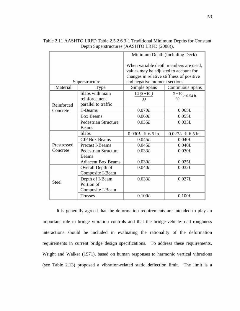
53
Table 2.11 AASHTO LRFD Table 2.5.2.6.3-1 Traditional Minimum Depths for Constant
Depth Superstructures (AASHTO LRFD (2008)).
Superstructure
Minimum Depth (Including Deck)
When variable depth members are used,
values may be adjusted to account for
changes in relative stiffness of positive
and negative moment sections
Material Type Simple Spans Continuous Spans
Reinforced
Concrete
Slabs with main
reinforcement
parallel to traffic
1.2 10
30
(S + )
100.54 ft.
30
S +
T-Beams 0.070L 0.065L
Box Beams 0.060L 0.055L
Pedestrian Structure
Beams
0.035L
0.033L
Prestressed
Concrete
Slabs 0.030L ≥ 6.5 in. 0.027L ≥ 6.5 in.
CIP Box Beams 0.045L 0.040L
Precast I-Beams 0.045L 0.040L
Pedestrian Structure
Beams
0.033L 0.030L
Adjacent Box Beams 0.030L 0.025L
Steel
Overall Depth of
Composite I-Beam
0.040L 0.032L
Depth of I-Beam
Portion of
Composite I-Beam
0.033L 0.027L
Trusses 0.100L 0.100L
It is generally agreed that the deformation requirements are intended to play an
important role in bridge vibration controls and that the bridge-vehicle-road roughness
interactions should be included in evaluating the rationality of the deformation
requirements in current bridge design specifications. To address these requirements,
Wright and Walker (1971), based on human responses to harmonic vertical vibrations
(see Table 2.13) proposed a vibration-related static deflection limit. The limit is a

54
computed transient peak acceleration of a bridge,
, it should not exceed 100
in /sec2,
where the static deflection, δs, is linked to
in such a way as:
s 0.05 L
(speed 0.3 fs L) fs Eq. 2.35
where,
L = span length; speed = vehicle speed; and
f s = natural frequency of a
simple span bridge, which may be estimated as:
fs
2L2
EbIb
m Eq. 2.36
where,
EbIb = flexural rigidity of a girder section;
m = unit mass of a girder
section. It should be noted that
s needs to be calculated for a live load with a girder
distribution factor of 0.7.
Nowak and Grouni (1988) also stated that the deflection and vibration criteria
should be derived by considering human reactions rather than structural performance. In
addition, similar efforts that relate static deflection limits to the natural frequency of a
bridge are shown in Canadian and Australian bridge design specifications (Ministry,
1991; CSA International, 2000; AUSTROADS, 1992, AUSTRALIAN, 1996). Figure 2.5
shows the relationship between the first flexural frequency (in Hz) and static deflections
limits (in mm) at the edge of a bridge from the Ontario Highway Bridge Design Code
(OHBDC). This was developed from extensive field data collection and analytical
models (Wright and Green, 1964). Figure 2.6 shows a similar relationship that is adopted
in the Australian Bridge Design Codes. It is worthy of pointing out that the static
deflection limits are usually absent in European bridge design specifications, and the

55
New Zealand Bridge Manual in 1994 limits the maximum vertical velocity to 2.2
in /sec
instead of using the maximum acceleration. Figure 2.7 shows the human perception to
particle velocities due to vibration (Oriard, 1972).
Debates on the necessity of deformation requirements in current bridge design
specifications focus on two aspects: (1) whether excessive deflections cause structural
damage; and (2) whether deflection limits provide effective controls of bridge vibrations
under normal traffic. Based on the limited survey in the ASCE report (1958), no
evidence of serious structural damage due to excessive vertical deflections was revealed.
However, unfavorable psychological reactions to bridge vibrations caused more concerns
on the subject of perceived bridge safety. Burke (2001) argued that if deflection limits
were not mandated, the effective service life of reinforced concrete deck slabs could
become considerably less than their normal replacement interval of 30 years. Moreover,
the report on NCHRP project 20-7 (Roeder et al., 2002) revealed that steel bridges clearly
suffered severe structural damage due to excessive deformation, but provided little
support for the idea that deflection limits should be used as a method of controlling these
structural damages. In addition, deflection limits were not considered as the “good”
method of controlling bridge vibrations (Azizinamini et al, 2004).

56
Table 2.12 Evolution of Deformation Requirements in Bridge Design
Year Agency Deflection
Limits
Span-to-Depth Ratio
Limits
1871 PBC 1/1,200 of span length
(at train speed: 30 mph)
1905 AREA 10 for trusses
10 for plate girders
12 for rolled beams and
channels
1907 AREA 10 for trusses
12 for plate girders
12 for rolled beams
1913 Bureau of
Public Roads
10 for trusses
12 for plate girders
20 for rolled beams
1919 AREA 10 for trusses
12 for plate girders
15 for rolled beams
1924 AASHO 10 for trusses
12 for plate girders
20 for rolled beams
1931 AASHO 10 for trusses
15 for plate girders
20 for rolled beams
1935 AASHO 10 for trusses
25 for plate girders
25 for rolled beams
1936 Bureau of
Public Roads
1/800 of span length
(for vibration controls)
1938 AASHO 1/800 of span length
1960 AASHTO 1/1000 of span length
(for pedestrian bridges)
Table 2.13 Peak Acceleration for Human Response to Harmonic Vertical Vibration
(Wright and Walker, 1971)
Human Response Transient Peak
Acceleration, in./sec2
Sustained Peak
Acceleration, in./sec2
Imperceptible 5 0.5
Perceptible to Some
Perceptible to Most
Perceptible
10
20
50
1
2
5
Unpleasant to Few
Unpleasant to Some
Unpleasant to Most
100
200
500
10
20
50
Intolerable to Some
Intolerable to Most
1000
2000
100
200
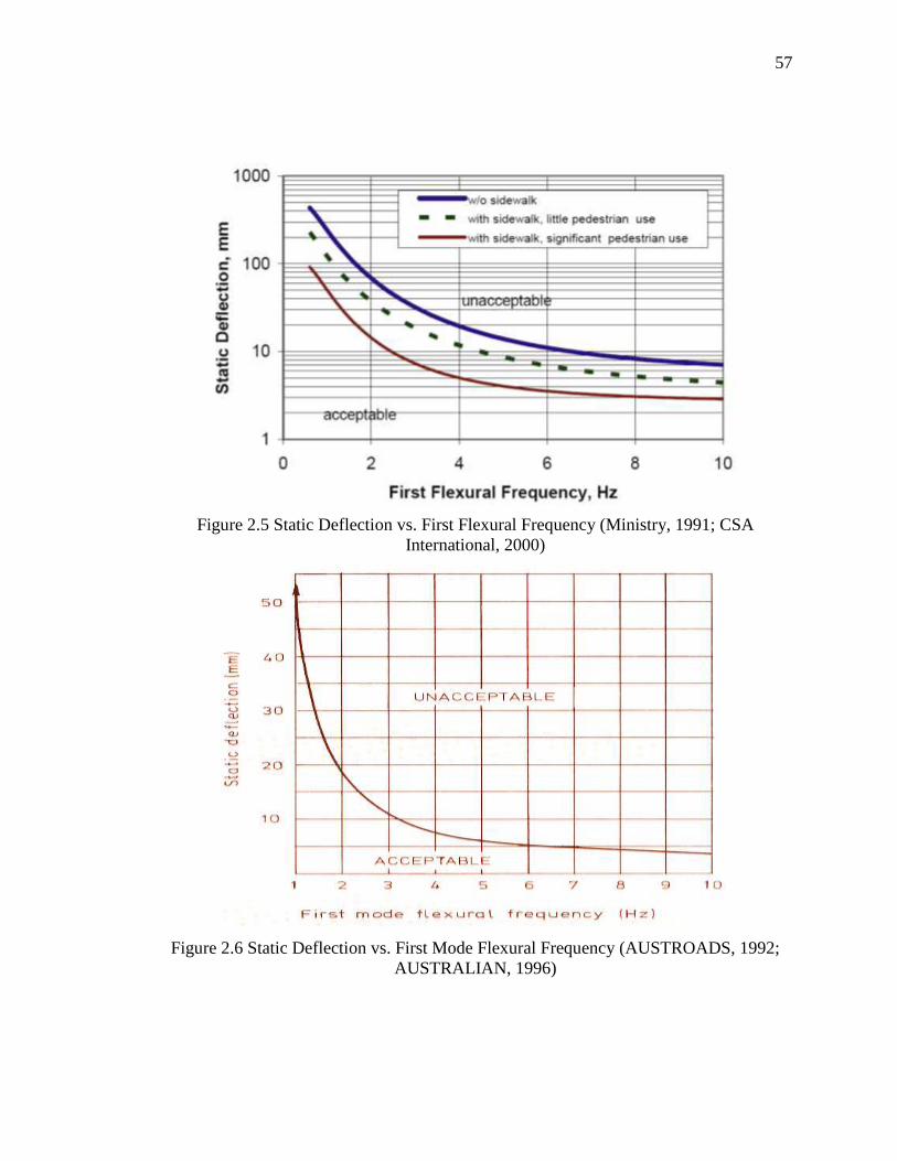
57
Figure 2.5 Static Deflection vs. First Flexural Frequency (Ministry, 1991; CSA
International, 2000)
Figure 2.6 Static Deflection vs. First Mode Flexural Frequency (AUSTROADS, 1992;
AUSTRALIAN, 1996)

58
Figure 2.7 Human Response to Particle Velocity (Oriard, 1972)
Debates on the necessity of deformation requirements in current bridge design
specifications focuses on two aspects: (1) whether excessive deflections cause structural
damage, and (2) whether the deflection limits provide effective controls of bridge
vibrations under normal traffic. Based on the limited survey in the ASCE report (1958),
no evidence of serious structural damage due to excessive vertical deflections was
revealed. However, unfavorable psychological reactions to bridge vibrations caused
more concerns on the subject of perceived bridge safety.
A comprehensive research was conducted by Wright and Walker (1971) to study
the factors regarding human perceptions and responses to bridge vibrations. The study
concluded that peak accelerations were preferable to peak velocities when evaluating
human perceptions to bridge vibrations that typically ranged from 1 to 10 Hz. Thus, a
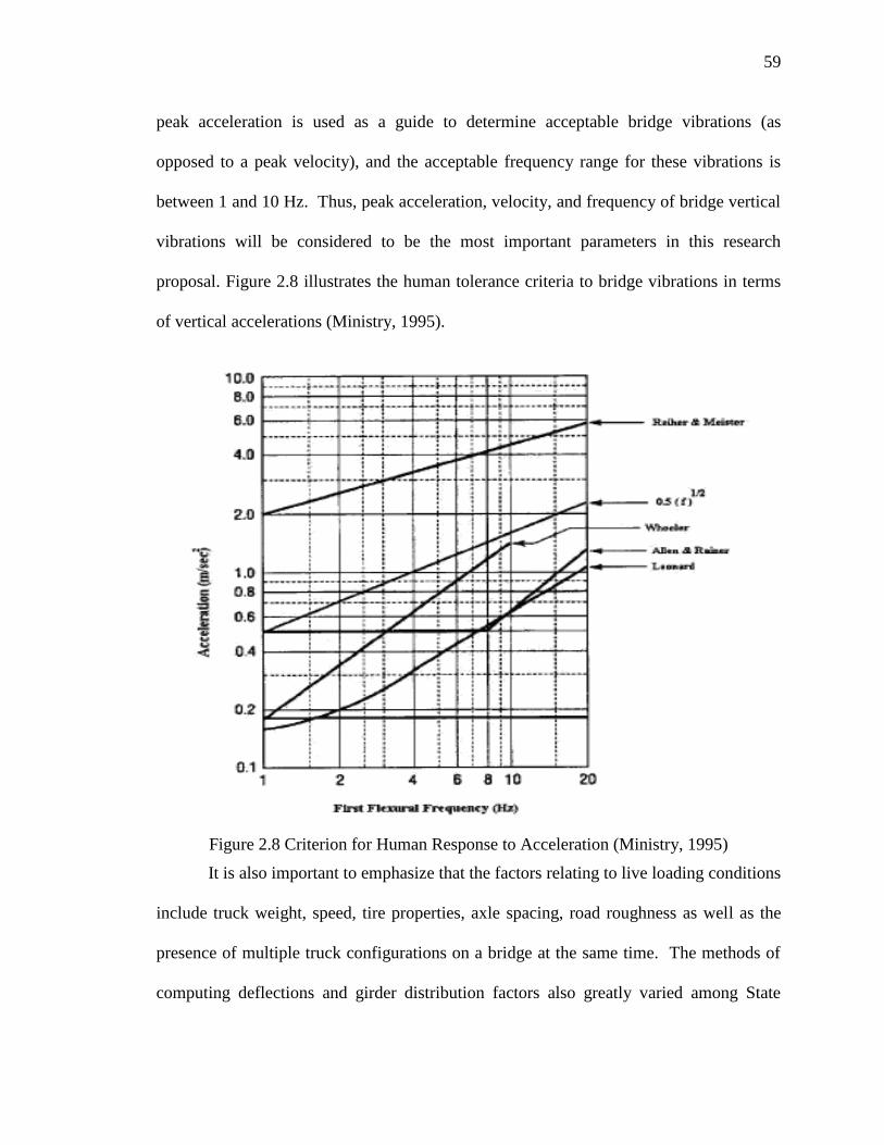
59
peak acceleration is used as a guide to determine acceptable bridge vibrations (as
opposed to a peak velocity), and the acceptable frequency range for these vibrations is
between 1 and 10 Hz. Thus, peak acceleration, velocity, and frequency of bridge vertical
vibrations will be considered to be the most important parameters in this research
proposal. Figure 2.8 illustrates the human tolerance criteria to bridge vibrations in terms
of vertical accelerations (Ministry, 1995).
Figure 2.8 Criterion for Human Response to Acceleration (Ministry, 1995)
It is also important to emphasize that the factors relating to live loading conditions
include truck weight, speed, tire properties, axle spacing, road roughness as well as the
presence of multiple truck configurations on a bridge at the same time. The methods of
computing deflections and girder distribution factors also greatly varied among State

60
Departments of Transportation (DOTs). For example, Wisconsin has a relatively low
legal load limit, 80 kips (356 kN), wherein it enforces the most strict deflection limit,
L 1600. The State of Michigan uses the standard
L 800 limit with the highest legal loads
in the United States, 164 kips (730 kN). In addition, impact and load factors were
applied in some States and not in others. These variations coupled with variable state
legal load limits resulted in an unknown, non-uniform level of safety for live-load
deflection serviceability criteria. Therefore, addressing live loading condition factors to
control deflection varies and becomes subjective.
In summary, it is clear that deformation requirements are necessary for both
prevention of structural damage and control of bridge vibrations. Furthermore, it is
believed that deformation requirements for bridge vibration control will be more
restrictive than those for prevention of structural damage. Therefore, there is a need to
focus future efforts of research on the establishment of the relationships between the
deformation requirements of deflection limits and corresponding span-to-depth ratio
limits and bridge vibration control.
61
3 MODELS FOR STRUCTURAL RESISTANCE AND
DEAD LOAD
CHAPTER 3
MODELS FOR STRUCTURAL RESISTANCE AND DEAD
LOAD
Due to the fact that the section properties of structures, material properties and even
construction procedures are subject to a great extent of uncertainty, a well-established
statistical model for structural resistance and dead load is critical for structural analysis.
Two steps should be taken for development of successful statistical models for structural
resistance. The first step is deriving a precise equation or numerical model that could
provide accurate estimation of structural resistance for various serviceability limit states.
Since each serviceability limit state represents different design criteria or “failure mode”,
the prediction equation or numerical model might be varied for each serviceability limit
state or performance levels, even for the same structure. Second step is to appropriately
extract the statistical information of structural resistance. This step involves selection of
appropriate reliability analysis techniques and estimation of statistical information for
each random variable involved. Utilizing appropriate reliability analysis technique, the
statistical model of resistance would be developed and can be used to predict the
reliability level of the structure.
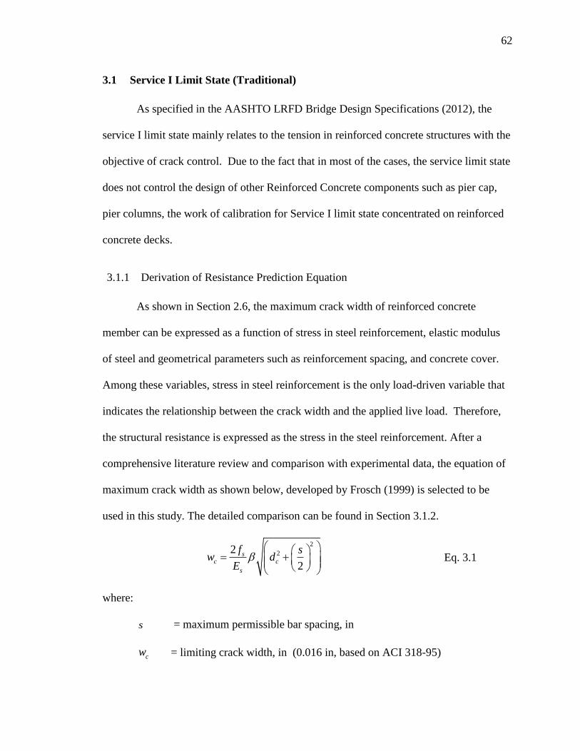
62
3.1 Service I Limit State (Traditional)
As specified in the AASHTO LRFD Bridge Design Specifications (2012), the
service I limit state mainly relates to the tension in reinforced concrete structures with the
objective of crack control. Due to the fact that in most of the cases, the service limit state
does not control the design of other Reinforced Concrete components such as pier cap,
pier columns, the work of calibration for Service I limit state concentrated on reinforced
concrete decks.
3.1.1 Derivation of Resistance Prediction Equation
As shown in Section 2.6, the maximum crack width of reinforced concrete
member can be expressed as a function of stress in steel reinforcement, elastic modulus
of steel and geometrical parameters such as reinforcement spacing, and concrete cover.
Among these variables, stress in steel reinforcement is the only load-driven variable that
indicates the relationship between the crack width and the applied live load. Therefore,
the structural resistance is expressed as the stress in the steel reinforcement. After a
comprehensive literature review and comparison with experimental data, the equation of
maximum crack width as shown below, developed by Frosch (1999) is selected to be
used in this study. The detailed comparison can be found in Section 3.1.2.
2
22
2
sc c
s
f sw d
E
Eq. 3.1
where:
s = maximum permissible bar spacing, in
cw
= limiting crack width, in (0.016 in, based on ACI 318-95)

63
sE
= Modulus of Elasticity of Steel, ksi
sf = Stress in Steel Reinforcement
= 1.0 + 0.08 cd
cd
= bottom cover measured from center of lowest bar, in
Rearranging terms in Eq. 3.1 to solve for sf as the resistance yields the following:
2
222
c ss
c
w Ef
sd
Eq. 3.2
The variables Es, β, and dc are random variables with statistical parameters. The
values wc and s are deterministic parameters based on ACI318-08 regulations of 0.016in
for wc and max 12(40000 / )sS f .
3.1.2 Comparison of Predication Equation for Maximum Crack Width of Reinforced
Concrete Members
As indicated in Section 3.1.1, an appropriate crack width prediction equation is important
for the accuracy of structural resistance. In this section, extensive literature review of the
research done on crack control from the 1950s to present is undertaken. The purpose of
the literature review is to understand the prior work (including code provisions) and
assess the influence of various parameters on crack control. It has been found that the
most contributing parameters are the steel stress, thickness of the concrete cover, and the
cross sectional area of concrete surrounding each bar. Moreover, the crack width on the
tension face is affected by the strain gradient from the level of steel to the tension face,
and that the bar diameter is not a major variable. Various code provisions and crack
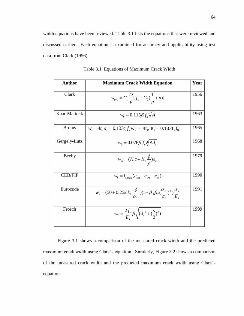
64
width equations have been reviewed. Table 3.1 lists the equations that were reviewed and
discussed earlier. Each equation is examined for accuracy and applicability using test
data from Clark (1956).
Table 3.1 Equations of Maximum Crack Width
Author Maximum Crack Width Equation Year
Clark 1 2
1[ ( )]ave s
Dw C f C n
p p
1956
Kaar-Mattock 40.115b sw f A 1963
Broms 4 0.133s e s e sw t t f 1965
Gergely-Lutz 30.076b s cw f Ad 1968
Beeby 1 2( )m mw K c K
1979
CEB/FIP ,max ( )k s sm cm csw l 1990
Eurocode 2
1 2 1 2(50 0.25 )(1 ( ) )sr sk
e f s s
w k kE
1991
Frosch 2 22
( ( ) )2
sc
s
f swc d
E
1999
Figure 3.1 shows a comparison of the measured crack width and the predicted
maximum crack width using Clark’s equation. Similarly, Figure 3.2 shows a comparison
of the measured crack width and the predicted maximum crack width using Clark’s
equation.

65
Figure 3.1 Comparison of the measured and predicted maximum crack width using
equation developed by Clark (1956).
Figure 3.2 Comparison between the measured and predicted maximum crack width using
equation developed by Karr and Mattock (1963).
0
0.005
0.01
0.015
0.02
0.025
0.03
0 0.005 0.01 0.015 0.02 0.025 0.03
Clark (fs=30 ksi)
Perfect Correlation
Clark (fs=45 ksi)
Pre
dic
ted
Max
imu
m C
rack
Wid
th (
in.)
Measured Maximum Crack Width (in.)
0
0.005
0.01
0.015
0.02
0.025
0.03
0 0.005 0.01 0.015 0.02 0.025 0.03
Karr and Mattock (fs=30ksi)
Perfect Correlation
Karr and Mattock (fs=45ksi)
Pre
dic
ted
Max
imu
m C
rack
Wid
th (
in.)
Measured Maximum Crack Width (in.)
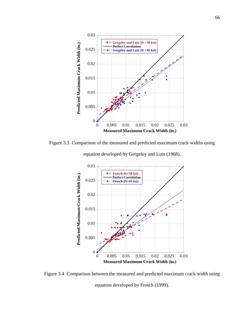
66
Figure 3.3 Comparison of the measured and predicted maximum crack widths using
equation developed by Gergeley and Lutz (1968).
Figure 3.4 Comparison between the measured and predicted maximum crack width using
equation developed by Frosch (1999).
0
0.005
0.01
0.015
0.02
0.025
0.03
0 0.005 0.01 0.015 0.02 0.025 0.03
Gergeley and Lutz (fs =30 ksi)
Perfect Correlation
Gergeley and Lutz (fs =45 ksi)
Pre
dic
ted
Max
imu
m C
rack
Wid
th (
in.)
Measured Maximum Crack Width (in.)
0
0.005
0.01
0.015
0.02
0.025
0.03
0 0.005 0.01 0.015 0.02 0.025 0.03
Frosch (fs=30 ksi)
Perfect Correlation
Frosch (fs=45 ksi)
Pre
dic
ted
Max
imu
m C
rack
Wid
th (
in.)
Measured Maximum Crack Width (in.)
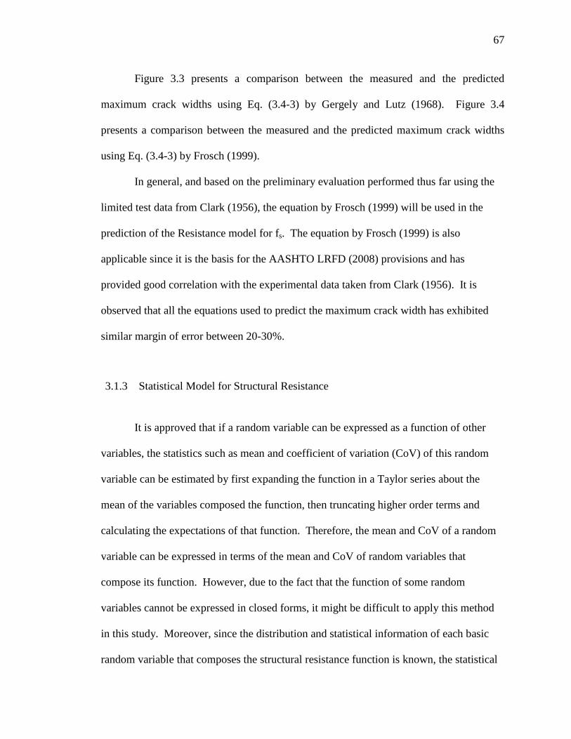
67
Figure 3.3 presents a comparison between the measured and the predicted
maximum crack widths using Eq. (3.4-3) by Gergely and Lutz (1968). Figure 3.4
presents a comparison between the measured and the predicted maximum crack widths
using Eq. (3.4-3) by Frosch (1999).
In general, and based on the preliminary evaluation performed thus far using the
limited test data from Clark (1956), the equation by Frosch (1999) will be used in the
prediction of the Resistance model for fs. The equation by Frosch (1999) is also
applicable since it is the basis for the AASHTO LRFD (2008) provisions and has
provided good correlation with the experimental data taken from Clark (1956). It is
observed that all the equations used to predict the maximum crack width has exhibited
similar margin of error between 20-30%.
3.1.3 Statistical Model for Structural Resistance
It is approved that if a random variable can be expressed as a function of other
variables, the statistics such as mean and coefficient of variation (CoV) of this random
variable can be estimated by first expanding the function in a Taylor series about the
mean of the variables composed the function, then truncating higher order terms and
calculating the expectations of that function. Therefore, the mean and CoV of a random
variable can be expressed in terms of the mean and CoV of random variables that
compose its function. However, due to the fact that the function of some random
variables cannot be expressed in closed forms, it might be difficult to apply this method
in this study. Moreover, since the distribution and statistical information of each basic
random variable that composes the structural resistance function is known, the statistical

68
model of structural resistance can be developed using Monte Carlo Simulation by
following the procedures below:
(1) A set of random numbers that have the value of either 0 or 1 is generated to
represent the probability of occurrence of the basic variables used in the
resistance prediction functions. It is important to note that the distributions of
all basic variables should be known.
(2) The corresponding random values of each basic variable can be obtained by
assigning the values generated in step 1 to its cumulative probability
distribution. Note that all random variables were generated independently in
accordance with their distribution.
(3) Based on the resistance prediction equation developed in Section 3.1.1,
calculate the structural resistance using the set of random values that
generated in step 2 for each random variable.
(4) Repeat step 1 to 3 to simulate a large sample database for the structural
resistance. The statistical information such as mean and CoV can be estimated
hereafter as the mean and CoV of the sample database.
It is important to point out that although the statistical model extracted from Monte-
Carlo simulation was based on the distribution and statistical information of each random
variable by its best estimation, due to the inherent randomness in each individual basic
variables, certain prediction error is expected and should be taken into account as part of
variability of structural resistance. Thus, the total CoV of structural resistance can be
estimated using the equation below:

69
Eq. 3.3
Where:
= total coefficient of variation of structural resistance
= value of coefficient of variation of structural resistance obtained from
Monte Carlo Simulation
= prediction error.
In this study, the prediction error of 0.1 is estimated from previous study
performed by Siriaksorn and Naaman (1980) regarding the crack control of reinforced
concrete members.
Table 3.2 Summary of Statistical Information for Random Variables for Service I Limit
State
Variable Distribution Mean CoV
As normal 0.9 A
sn 0.015
b normal bn 0.04
CEc
normal 33.6 0.1217
d normal dn
0.06
dc normal d
cn 0.06
Es normal E
sn 0.024
¢fc
lognormal
cE = CEc
1.5 '
c cf
(psi) 3000: 1.31
cnf
3500:1.27 cnf
4000: 1.24 cnf
4500: 1.21 cnf
5000: 1.19 cnf
3000: 0.17
3500: 0.16
4000: 0.15
4500:0.14
5000:0.135
fy lognormal 1.13 f
yn 0.03
h normal hn 1/ 6.4
gc normal 150 pcf 0.03
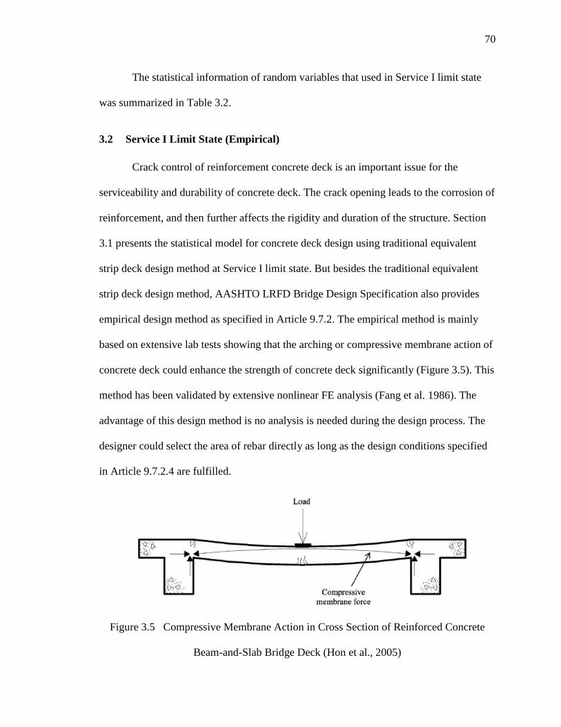
70
The statistical information of random variables that used in Service I limit state
was summarized in Table 3.2.
3.2 Service I Limit State (Empirical)
Crack control of reinforcement concrete deck is an important issue for the
serviceability and durability of concrete deck. The crack opening leads to the corrosion of
reinforcement, and then further affects the rigidity and duration of the structure. Section
3.1 presents the statistical model for concrete deck design using traditional equivalent
strip deck design method at Service I limit state. But besides the traditional equivalent
strip deck design method, AASHTO LRFD Bridge Design Specification also provides
empirical design method as specified in Article 9.7.2. The empirical method is mainly
based on extensive lab tests showing that the arching or compressive membrane action of
concrete deck could enhance the strength of concrete deck significantly (Figure 3.5). This
method has been validated by extensive nonlinear FE analysis (Fang et al. 1986). The
advantage of this design method is no analysis is needed during the design process. The
designer could select the area of rebar directly as long as the design conditions specified
in Article 9.7.2.4 are fulfilled.
Figure 3.5 Compressive Membrane Action in Cross Section of Reinforced Concrete
Beam-and-Slab Bridge Deck (Hon et al., 2005)
71
Unlike the reinforced concrete deck designed using traditional method, the moment
resistance of reinforced concrete deck designed using empirical method contains two
components: (1) resistance due to tension of the concrete and reinforcement at the bottom
fiber of the concrete deck at positive moment region, and (2) resistance due to arching
action at the positive moment region. It is noteworthy that the arching action only
contributes to the resistance at positive moment area. In this section, sub-section 3.2.1
presents the comprehensive investigation of arching action mechanism has been
conducted by the author. Sub-section 3.2.1 presents the resistance predication equation at
both positive moment and negative moment region for concrete deck designed using
empirical method. Sub-section 3.2.3 presents the statistical model of structural resistance
for concrete deck designed using empirical method at Service I limit state.
3.2.1 Investigation of Arching Action of Concrete Deck
An early study regarding the ultimate strength and arching action effect of
concrete was conducted by Park (1964). The author proposed a method to analyze the
ultimate strength of rectangular concrete slabs based on plastic theory.
Tsui et al. (1986) studied the load capacity of the Ontario-type bridge deck on
steel girders. A full-size composite bridge, in which half of it had a cast-in-place deck
and another half had precast, prestressed panels, were tested with a series of static loads,
5 million cycles of fatigue loading, and concentrated load. Besides the experimental
study, the finite element model was developed and the results were compared with the
experimental results. The experimental results revealed that the precast, prestressed panel
deck was stronger and provided better crack-resistant than the cast-in-place deck.
72
Guice and Rhomberg (1988) tested 16 one-way reinforced concrete slab strips to
investigate the effects of the restraints. The author concluded that adequate lateral
stiffness is required to develop both compressive and tensile membrane enhancements.
The author also concluded that the small rotational freedoms do not significantly affect
the compressive membrane capacity, but enhance the tensile membrane capacity.
Fang et al. (1990a, 1990
b, 1990
c, 1994) conducted a series of study regarding the
load capacity and fatigue behavior of Ontario-type reinforced concrete bridge decks. A
full-scale Ontario-type bridge deck reinforced with about 60% of the reinforcement
required by AASHTO Code was tested under service and overload conditions. The
experimental results showed that the membrane action did not noticeably affect the
performance of the deck prior to deck cracking but the flexural capacity of the deck was
increased significantly due to the arching action of the bridge deck. The authors also
concluded that both the ACI and AASHTO punching shear formulas were very
conservative.
Rankin and Long (1997) performed a series of study regarding the compressive
membrane action and strength enhancement of concrete slabs. They summarized the
mechanism of arching action and proposed a method to calculate the strength
enhancement. The steps for calculating the arching moment are summarized as follows:
(1) Horizontal translational restraint stiffness of concrete deck, K:
The horizontal translational restraint stiffness is an essential parameter to estimate
the flexural capacity enhancement due to arching action. Rankin and Long (2003)
proposed the following equation to compute the translational restraint stiffness of
concrete deck:

73
b
e
EAK
L Eq. 3.4
Where,
E = The modulus of elasticity of the edge beams,
bA = The equivalent area of the lateral stiffness,
eL = half span of elastically-restrained strip, / 2eL L .
(2) Depth available for arching, d1:
'
1
( )0.85
2
sy
c
c
f dD p p
fd
Eq. 3.5
Where,
D = The overall depth of the deck,
syf = The yield strength of reinforcement,
p = The positive reinforcement ratio,
cp = The negative reinforcement ratio,
d = The effective depth of the deck,
'
cf = Compressive strength of the concrete,
(3) Equivalent length of rigidly restrained arch, rL :
1/3
1cr e
e
E AL L
KL
Eq. 3.6
Where,
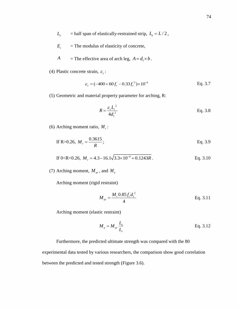
74
eL = half span of elastically-restrained strip, / 2eL L ,
cE = The modulus of elasticity of concrete,
A = The effective area of arch leg, 1A d b .
(4) Plastic concrete strain, c :
' '2 6( 400 60 0.33 ) 10c c cf f Eq. 3.7
(5) Geometric and material property parameter for arching, R:
2
2
14
c rLR
d
Eq. 3.8
(6) Arching moment ratio, rM :
If R>0.26, 0.3615
rMR
; Eq. 3.9
If 0<R<0.26, 44.3 16.1 3.3 10 0.1243rM R . Eq. 3.10
(7) Arching moment, arM , and aM
Arching moment (rigid restraint)
' 2
10.85
4
r car
M f dM Eq. 3.11
Arching moment (elastic restraint)
ea ar
r
LM M
L Eq. 3.12
Furthermore, the predicted ultimate strength was compared with the 80
experimental data tested by various researchers, the comparison show good correlation
between the predicted and tested strength (Figure 3.6).

75
Figure 3.6 Correlation of Predictions with test results (Rankin and Long, 1997)
Bailey (2000) performed a study on the membrane action of unrestrained lightly
reinforced concrete slabs at large displacement. The author conducted six compartment
tests on a full-scale, eight story, steel frame building. The fire resistance and flexural
behavior were investigated through the tests. The author decided to ignore any horizontal
restraint to simplify the analysis. Based on the experimental results and analytical study,
the author proposed a new theoretical approach to predict the load capacity of the slab at
large displacement. Furthermore, the author compared the predicted results with
published test data. The comparison indicates the prediction has excellent correlation
with the test data.
Peel-Cross et al. (2000) conducted an experimental study of the ultimate load
capacity of composite slabs. The experimental results demonstrated the compressive
membrane effects significantly increase the load capacity of interior floor panels but with
less contribution to the edge panels.

76
Taylor et al. (2001) tested 15 reinforced concrete slab strips constructed with
high-strength concrete. The testing results indicated that the degree of external lateral
restraint and the concrete compressive strength have significant effects on the strength of
laterally restrained slabs.
Graddy et al. (2002) conducted a study regarding the punching-shear behavior of
bridge decks under fatigue loading. Static and pulsating fatigue tests were performed on
full-scale, cast-in-place and precast, prestressed panel specimens. The experimental data
were compared with analytical predictions. The finite element models were also
developed and the prediction was also compared with the experimental data. The authors
concluded that the punching shear capacity predicted by AASHTO and ACI equation was
conservative compared to the experimental data and arching action results in insignificant
increase in flexural capacity of simply supported slabs.
Salim and Sebastian (2003) conducted an experimental study of the ultimate
punching load capacity of reinforced concrete slabs. Four reinforced concrete slabs were
tested in this study. Moreover, the authors proposed a theoretical method to predict the
punching shear failure loads using plasticity theory. The predictions provided good
agreement with the experimental data from the literature.
Hon et al. (2005) performed 8 punching shear failure tests and 15 flexural failure
tests. They also adopted the method proposed by Rankin and Long (1997) in their study
to predict the load capacity of the concrete slabs. The comparison between the
experimental data and prediction shows both Rankin and Long (1997) and FE analysis
shows good prediction (Figure 3.7).

77
Figure 3.7 Comparison between peak loads for flexural failure tests (Hon et al.,
2005)
Taylor et al. (2007) evaluated the serviceability of bridge deck slabs with arching
action. The measured crack widths, deflections and the load capacity collected from the
tests on a full scale bridge deck were compared with the current code requirements. The
comparison indicates the UK code overestimated the crack widths in various loading
level and ignored the beneficial effects of arching action. The comparison also shows
both the ACI and BS codes give similar and conservative prediction for the strength of
concrete slabs.
Bailey et al. (2008) tested 14 horizontally unrestrained concrete slabs with large
vertical deflection. A simple approach was developed based on rigid-plastic behavior.
The proposed approach provided good prediction of load-displacement response
compared with the experimental results. Additionally, a finite element model (FEM) was
developed and compared with the experimental data. The comparison indicated the FEM
can be used to predict the load capacity of horizontally unrestrained concrete slabs.

78
Meadway (2008) conducted a comprehensive study to evaluate the current deck
design practice. The author performed the laboratory test on four full scale models. A
finite element model was developed and validated with the experimental data. A
parametric study was performed using the validated finite element model. The author
concluded that the strength of the concrete deck decrease by approximately 50 kips when
the span length increased from 6 ft to 12 ft.
Schmeckpeper et al. (2010) investigated the effect of bridge deck design
methodology on crack control. The authors reviewed the literature regarding the effect of
bridge deck design methodology on deck cracking. They also surveyed all the states
agencies regarding the bridge deck design methods. They believe the cracking problem
can be better controlled by reducing the spacing and increasing the rebar size but further
research needs to be conducted prior to providing detailed recommendations.
3.2.2 Derivation of Resistance Prediction Equation
Similar to the resistance prediction equation for concrete deck designed using
traditional design method, the resistance due to the tension of reinforcement can be
expressed as Eq. 3.2. At positive moment region, the resistance due to arching action can
be expressed as:
2 2' 2
1
3 3 2 0.85
(4 9 ) 4
s s c s s s s cr c
s
s s c s
A E E bd A E A E E bd M f df
d A E E bd A
Eq. 3.13
Therefore, total resistance at the positive moment region can be calculated using
the equation below:
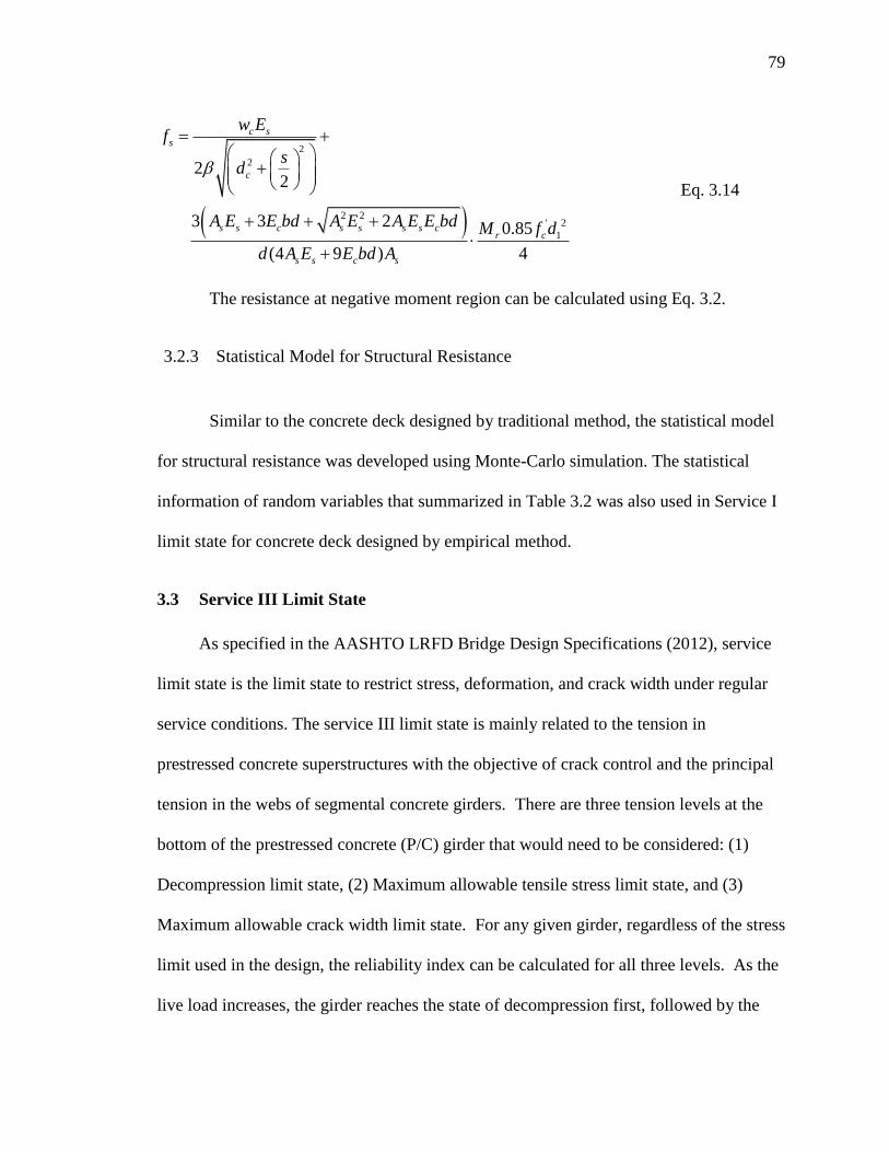
79
2
2
2 2' 2
1
22
3 3 2 0.85
(4 9 ) 4
c ss
c
s s c s s s s cr c
s s c s
w Ef
sd
A E E bd A E A E E bd M f d
d A E E bd A
Eq. 3.14
The resistance at negative moment region can be calculated using Eq. 3.2.
3.2.3 Statistical Model for Structural Resistance
Similar to the concrete deck designed by traditional method, the statistical model
for structural resistance was developed using Monte-Carlo simulation. The statistical
information of random variables that summarized in Table 3.2 was also used in Service I
limit state for concrete deck designed by empirical method.
3.3 Service III Limit State
As specified in the AASHTO LRFD Bridge Design Specifications (2012), service
limit state is the limit state to restrict stress, deformation, and crack width under regular
service conditions. The service III limit state is mainly related to the tension in
prestressed concrete superstructures with the objective of crack control and the principal
tension in the webs of segmental concrete girders. There are three tension levels at the
bottom of the prestressed concrete (P/C) girder that would need to be considered: (1)
Decompression limit state, (2) Maximum allowable tensile stress limit state, and (3)
Maximum allowable crack width limit state. For any given girder, regardless of the stress
limit used in the design, the reliability index can be calculated for all three levels. As the
live load increases, the girder reaches the state of decompression first, followed by the

80
tensile stress increasing until it reaches the prescribed cracking limit causing the concrete
to crack. After cracking, the width of the crack increases until it reaches the prescribed
crack width limit.
Similar to crack control of Service I limit state, the tension level at the bottom of
concrete girder can be expressed by the tension in prestressing strands. Thus, the stresses
in the prestressing strands were used as the resistances for Service III limit state for
prestressed concrete girder in this study. In this section, sub-section 3.3.1 presents the
derivation of the resistance prediction equation at three tension levels. Since the accuracy
of the crack width prediction equation directly affects the accuracy of resistance
estimation after the crack occurs at the bottom of prestressed concrete girder, sub-section
3.3.2 presents the comprehensive investigation and comparison of maximum crack width
prediction equation at the bottom of prestressed concrete girder. Finally, Sub-section
3.2.3 presents the statistical model of structural resistance for prestressed concrete girders
at Service III limit state.
3.3.1 Derivation of Resistance Prediction Equation
The derivation of the resistance prediction equation for a prestressed concrete
girder subjected to flexural loading is shown in this section. Figure 3.8 shows the stress
distribution diagram for a typical prestressed concrete bridge girder at various stages of
loading.

81
Ten
sio
nC
om
pre
ssio
nC
om
pre
ssio
nC
om
pre
ssio
n
Co
mpre
ssio
nC
om
pre
ssio
nT
ensi
on
(a)
Init
ial
Sta
te(b
) D
ead
Load
Sta
te
Co
mpre
ssio
n
(c)
Dec
om
pre
ssio
n
@ B
ott
om
of
Gir
der
(d)
Dec
om
pre
ssio
n
@ L
evel
of
Pre
stre
ssin
g(e
) S
erv
ice
Lo
ad S
tate
b
hf2
hf1hf
b0
bw
b1
hd
sd
p
c
Fig
ure
3.8
S
tres
s D
istr
ibuti
on D
iagra
ms
for
a T
ypic
al P
rest
ress
ed C
oncr
ete
Bri
dge
Gir
der
at
Var
ious
Sta
ges
of
Lo
adin
g

82
Using force equilibrium:
0 02 ( )( )
2
f
ctps ps s s f ct
c h
fA f A f b c b b c h f
c
1
12 ( )( )
f f
w f f ct
c h h
b b c h h fc
2 2 2
0 0 1( ) ( ) ( ) ( )2
ctf f f w
fb c c h b b c h h b b
c Eq. 3.15
where,
sA = area of non-prestressing steel
psA = area of prestressing steel in tension zone
b = prestressed beam top flange width
0b = effective deck width transformed to the beam material
wb = web thickness
c = depth of neutral axis from the from extreme compression fiber
ctf = calculated stress in concrete at the top fiber.
psf = calculated stress in prestressing steel.
sf = calculated stress in non-prestressing steel.
fh = deck thickness
1fh = top flange thickness
The stress in the prestressing steel can be calculated as follows:
( ) ( )ps p
ps ps ps ps se ce ct
c
E d cf E E f
E c
Eq. 3.16
By rearranging Eq. 3.16, the stress in the concrete at the top fiber can be
calculated as follows:

83
( )
( )
ps ps se ce c
ct
ps p
f E E cf
E d c
Eq. 3.17
From strain compatibility,
( )s ss s s ct
c
E d cf E f
E c
Eq. 3.18
where,
c = depth of neutral axis from the from extreme compression fiber
pd
= the distance from extreme compression fiber to centroid of
prestressing steel.
sd
= the distance from extreme compression fiber to centroid of non-
prestressing steel.
cE = modulus of elasticity of concrete
psE = modulus of elasticity of prestressing steel
sE = modulus of elasticity of non-prestressing steel
ctf = stress in the concrete at the top of the beam after losses at service
load
ce = strain in concrete at the level of prestressing steel after losses at
dead load state
ps = strain in prestressing steel after losses at service load
s = strain in non-prestressing steel after losses at service load
se = strain in prestressing steel after losses at dead load state
Substitute Eq. 3.17 and Eq. 3.18 into Eq. 3.15:

84
( )
2 ( )
ps ps se ce c
ps ps
ps p
f E EA f
E d c
2 2 2
0 0 1
2 ( )( ) ( ) ( ) ( ) s s s
f f f w
c
A E d cb c c h b b c h h b b
E
Eq. 3.19
Eq. 3.19 can be simplified and rewritten as a quadratic equation with unknown c,
neutral axis depth, as follows:
2
0 1 1
2
( )
ps ps ps s sf f w f w f
w cps ps se ce c
A f E A Ec b h bh b h b h c
b Ef E E
2 2
0 1
2 1 1( ) ( )( ) 0
2 2( )
ps ps ps s s sf w f f
w cps ps se ce c
A f E A E db b h b b h h
b Ef E E
Eq. 3.20
The moment resistance can be expressed as follows:
2
02
0
( ) ( ) 21( )
6 2 3
f f
n ps ps p s s s ct ct
c h b b c hM A f d A f d f b c f
c
2
1 1( ) ( ) 2 2( )
2 3
f f w f f
ct
c h h b b c h hf
c
Eq. 3.21
where,
nM = nominal moment resistance.
sf is calculated using equation Eq. 3.18, and
ctf is calculated using equation Eq.
3.17.
The depth of neutral axis from the compression face, c, can be computed using
Eq. 3.20.
Also, assuming linear elastic relationship in the behavior of the prestressing steel:

85
sese
ps
f
E
Eq. 3.22
Then,
2
0 01( )
ps se Dce
c c c
A f e M e
E A I E I
Eq. 3.23
where,
cA = area of concrete at the cross-section considered.
0e = eccentricity of the prestressing force with respect to the centroid of the
section at mid span.
cE = modulus of elasticity of concrete.
psE = modulus of elasticity of prestressing steel.
sef = effective stress in prestressing steel after losses.
I = moment of inertia.
DM = dead load moment.
If we consider uncracked section behavior under service loads, and plane section
remains plane, then the linear strain distribution diagram is as follows:
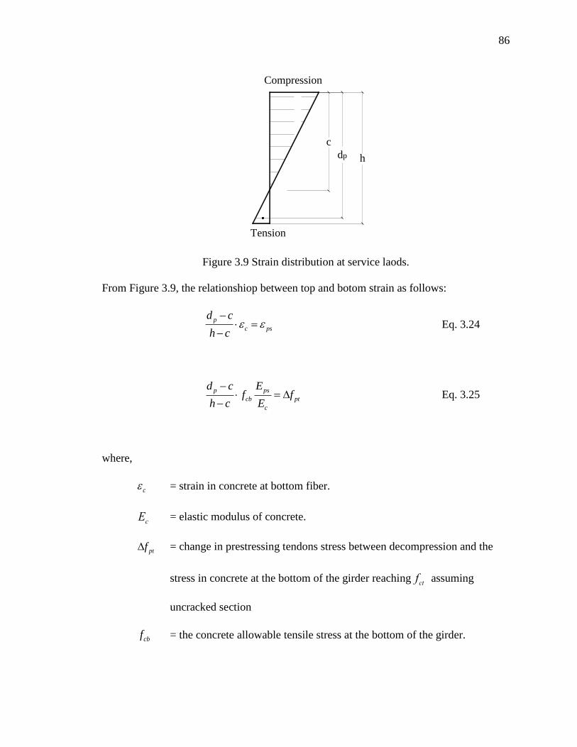
86
Figure 3.9 Strain distribution at service laods.
From Figure 3.9, the relationshiop between top and botom strain as follows:
p
c ps
d c
h c
Eq. 3.24
p ps
cb pt
c
d c Ef f
h c E
Eq. 3.25
where,
c = strain in concrete at bottom fiber.
cE = elastic modulus of concrete.
ptf = change in prestressing tendons stress between decompression and the
stress in concrete at the bottom of the girder reachingctf assuming
uncracked section
cbf = the concrete allowable tensile stress at the bottom of the girder.
Compression
Tension
dp h
c

87
According to the current AASHTO LRFD (2012) Specifications, =0.19cb cf f or
=0.0948cb cf f , which is depends on the exposure conditions.
Then psf for maximum tensile stress limit level (uncracked section) should be as
follows:
t ( )Decps p ps Mf f f
Eq. 3.26
For the section at the maximum crack width limit level (cracked section), the psf
can be calculated by the following equation:
( )Decps ps ps Mf f f Eq. 3.27
where
( )Decps Mf = the stress in prestressing steel at decompression
psf = the increase in the prestressing steel stress beyond the decompression
state for cracked members.
DecM
= the decompression moment.
tpf will vary according to the maximum allowable tensile stress at the bottom of
the concrete girder.
Moreover, psf at decompression level, which expressed as ( )Decps Mf can be calculated
using the following equation:
( ) 2
0
[ ]
1[1 ( )]
Dec
ps Dec D
ps M seps ps
c
c c
E M Mf f
A E eIE
E A I
Eq. 3.28

88
The decompression moment at level of prestressing strands, DecpM , can be
calculated using the following equation:
0
2
0
00
2 2
0 0
[ ]1
[ ( )]
1 1[ ] [1 ( )]
D ps
seps ps
c
c cDecp
ps
ps ps
ps c
c c c
M e Ef
A E eI IE
E A IM
e Ee
A Ee eI A IE
A I E A I
Eq. 3.29
The decompression moment at bottom fiber of concrete girder, DecbM , can be
calculated using the following equation:
0
2
0
0
20 0
[ ]1
[ ( )]
1 1[ ] [1 ( )]
D ps
seps ps
c
c cDecb
psb
b ps psps c
c c c
M e Ef
A E eI IE
E A IM
e Ey
e y A E eI A IE
A I E A I
Eq. 3.30
where,
cA = area of concrete at the cross-section considered.
psA = the area of prestressing steel in tension zone.
0e = eccentricity of the prestressing force with respect to the centroid of the
section at mid-span.
by = Distance from centroidal axis to extreme bottom fiber
cE = modulus of elasticity of concrete.
psE = modulus of elasticity of prestressing steel.

89
sef = effective stress in prestressing steel after losses.
I = moment of inertia.
DM = dead load moment.
DecbM = decompression moment at the bottom of the girder.
DecpM = decompression moment at the level of the prestressing strands.
3.3.2 Comparison of Predication Equation for Maximum Crack Width at bottom fiber
of Prestressed Concrete Girders
This section presents a review and a comparison of various prediction equations
for the maximum crack width in prestressed concrete members. Test data from various
sources were used in the comparisons. The equations below are listed in chronological
order:
The 1970 CEB-FIP recommended adopting the following equation to predict the
maximum crack width in partially prestressed beams:
6
max ( 4000) 10sw f
Eq. 3.31
For static loads, the equation is:
6
max 10sw f
Eq. 3.32
Please note that the sf in the CEB-FIP equation is in N/cm2.
Nawy and Potyondy (1971) conducted a research program to study the flexural
cracking behavior of pretensioned I and T beams. Table 3.3 shows the geometric and
mechanical properties of the prestressed beam specimens. sA represents the area of
tension reinforcement comprising both prestressing and normal steel reinforcement and

90
'
sA represents the area of compression steel reinforcement. f’c is the concrete cylinder
compressive strength and f’t is the concrete tensile splitting strength.
Table 3.3 Geometrical Properties of the Prestressed Beams (Nawy and Potyondy,1971)
Beam Section Width
b, in.
Depth*
d, in. sA
sq in.
sA
bd
Percent
'
sA
sq
in.
'' sA
bd
Percent
f’c
psi
f’t psi
Slump
in.
B1 T 8 8.75 0.271 0.389 - - 4865 400 3
B2 I 6 8.90 0.271 0.518 - - 4865 400 3
B3 T 8 8.75 0.271 .0389 - - 4330 430 4
B4 I 6 8.90 0.271 0.518 - - 4290 430 4
B5 I 6 8.90 0.271 0.518 - - 4340 430 4
B6 T 8 8.75 0.271 0.389 - - 4375 430 4
B7 T 8 8.75 0.271 0.389 - - 4290 390 6
B8 I 6 8.90 0.271 0.518 - - 4260 390 6
B9 I 6 8.90 0.271 0.518 - - 4190 390 6
B10 T 8 8.75 0.271 0.389 - - 4280 390 6
B11 T 8 8.75 0.271 0.389 - - 4150 370 8
B12 I 6 8.90 0.271 0.518 - - 3920 370 8
B13 I 6 8.90 0.281 0.518 - - 3890 370 8
B14 T 8 8.75 0.271 0.389 - - 4110 370 8
B15 T 8 8.75 0.271 0.389 0.93 1.332 3490 340 5 1/2
B16 I 6 8.90 0.271 0.518 0.33 0.631 3400 340 5 1/2
B17 I 6 8.90 0.271 0.518 0.93 1.776 3390 340 5 1/2
B18 T 8 8.75 0.271 0.389 0.33 0.473 3510 340 5 1/2
B19*
* I 6 8.90 0.235 0.448 - - 3610 385 6
B20*
* I 6 8.90 0.235 0.448 - - 3495 385 6
B21*
* I 6 8.90 0.235 0.448 - - 3430 355 6 1/2
B22*
* I 6 8.90 0.235 0.448 - - 3280 355 6 1/2
B23 I 6 8.90 0.271 0.518 - - 4060 380 5
B24 I 6 8.90 0.271 0.518 - - 4095 380 5
B25 I 6 8.90 0.271 0.518 - - 3950 380 5
B26 I 6 8.90 0.271 0.518 - - 4000 380 5
* Total depth h in each beam = 12 in.
+ As includes two 3/16 in. diameter normal high strength steel wire (fy = 96,000 psi)
cage bars in addition to prestressing tendons.
** Beams B19-B22 were continuous beams and were not included in the cracking
analysis
91
Based on a regression analysis of the test data, the authors proposed the following
prediction equation:
1/4
6 3
max 11.13 10 tc s
s
Aw a f
A
Eq. 3.33
where,
1sf = 3.75s df f , ksi
ca = stabilized crack spacing, in.
tA = area of concrete in tension, in
2.
sA = total area of reinforcement, in
2.
E = 27.5×10³ ksi was used.
sf = stress in prestressing steel after cracking, ksi.
df = stress in the prestressing steel when the modulus of rupture of concrete at the
extreme tensile fibers is reached, ksi.
After further simplification of Eq. 3.31, Nawy and Potyondy (1971)
recommended the following expression:
max 1.44 8.3sw f ( )
Eq. 3.34
Please note the unit for sf in Eq. 3.31 is in ksi and the unit for crack width is in
inches.
Bennett and Veerasubramanian (1972) investigated the behavior of non-
rectangular beams with limited prestress after flexural cracking. They tested 34
prestressed concrete beams with the cross-section and loading arrangement shown in
Figure 3.10.
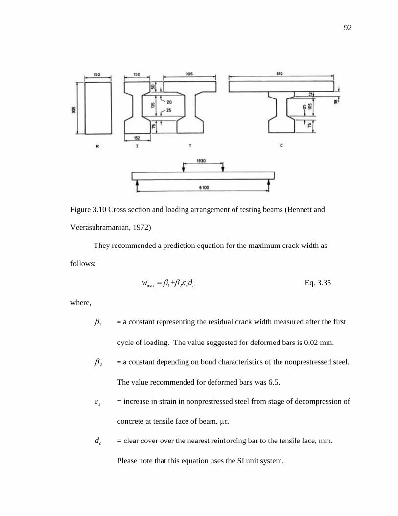
92
Figure 3.10 Cross section and loading arrangement of testing beams (Bennett and
Veerasubramanian, 1972)
They recommended a prediction equation for the maximum crack width as
follows:
max 1 2+ s cw d
Eq. 3.35
where,
1 = a constant representing the residual crack width measured after the first
cycle of loading. The value suggested for deformed bars is 0.02 mm.
2 = a constant depending on bond characteristics of the nonprestressed steel.
The value recommended for deformed bars was 6.5.
s = increase in strain in nonprestressed steel from stage of decompression of
concrete at tensile face of beam, µε.
cd = clear cover over the nearest reinforcing bar to the tensile face, mm.
Please note that this equation uses the SI unit system.
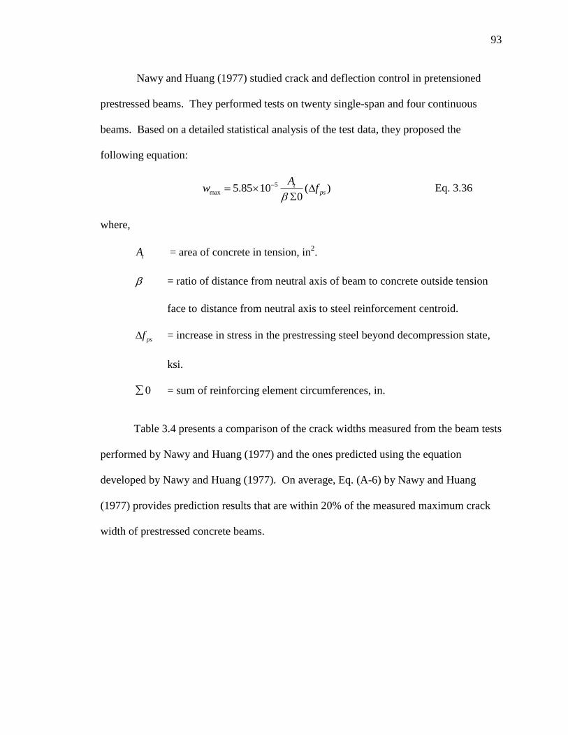
93
Nawy and Huang (1977) studied crack and deflection control in pretensioned
prestressed beams. They performed tests on twenty single-span and four continuous
beams. Based on a detailed statistical analysis of the test data, they proposed the
following equation:
5
max 5.85 10 ( )0
tps
Aw f
Eq. 3.36
where,
tA = area of concrete in tension, in2.
= ratio of distance from neutral axis of beam to concrete outside tension
face to distance from neutral axis to steel reinforcement centroid.
psf = increase in stress in the prestressing steel beyond decompression state,
ksi.
0 = sum of reinforcing element circumferences, in.
Table 3.4 presents a comparison of the crack widths measured from the beam tests
performed by Nawy and Huang (1977) and the ones predicted using the equation
developed by Nawy and Huang (1977). On average, Eq. (A-6) by Nawy and Huang
(1977) provides prediction results that are within 20% of the measured maximum crack
width of prestressed concrete beams.

94
Table 3.4 Observed vs. theoretical max. crack width at tensile face of beam (Nawy and
Huang, 1977)
Net steel stress
30 ksi 40 ksi 60 ksi 80 ksi
wobs. wtheory Error
% wobs. wtheory
Error
% wobs. wtheory
Error
% wobs. wtheory
Error
%
0.0111 0.0131 -15.3 0.0151 0.0175 -13.7 0.0261 0.0262 -0.4 0.04 0.0349 14.6
0.0127 0.0118 7.6 0.0204 0.0157 29.9 0.0275 0.0236 16.5 0.0409 0.0313 30.7
0.0131 0.0128 2.3 0.0166 0.0172 -3.5 0.0304 0.0256 18.8 0.0382 0.0344 11.0
0.0097 0.013 -25.4 0.0158 0.0174 -9.2 0.0226 0.0259 -12.7 0.0304 0.0347 -12.4
0.0091 0.0147 -38.1 0.0117 0.0197 -40.6 0.0205 0.0294 -30.3 0.032 0.0393 -18.6
0.0124 0.0148 -16.2 0.0181 0.0199 -9.0 0.0213 0.0297 -28.3 0.0364 0.0397 -8.3
0.0052 0.0051 2.0 0.0068 0.0069 -1.4 0.0117 0.0103 13.6 0.0188 0.0137 37.2
0.0049 0.0051 -3.9 0.0061 0.0069 -11.6 0.0111 0.0103 7.8 0.0146 0.0137 6.6
0.0051 0.0045 13.3 0.0064 0.0061 4.9 0.0107 0.009 18.9 0.0165 0.0121 36.4
0.0058 0.0045 28.9 0.0082 0.0061 34.4 0.0134 0.009 48.9 0.0185 0.0121 52.9
0.0054 0.0059 -8.5 0.0069 0.0079 -12.7 0.0112 0.0119 -5.9 0.0172 0.0158 8.9
0.0048 0.0059 -18.6 0.0076 0.0079 -3.8 0.0134 0.0119 12.6 0.0192 0.0158 21.5
0.0043 0.0046 -6.5 0.0058 0.0062 -6.5 0.0105 0.0092 14.1 0.0138 0.0123 12.2
0.0052 0.0046 13.0 0.0059 0.0062 -4.8 0.0103 0.0092 12.0 0.0145 0.0123 17.9
0.0039 0.0057 -31.6 0.0061 0.0076 -19.7 0.0115 0.0114 0.9 0.0181 0.0153 18.3
0.0038 0.0057 -33.3 0.0057 0.0076 -25.0 0.0093 0.0114 -18.4 0.016 0.0153 4.6
0.0039 0.0056 -30.4 0.006 0.0074 -18.9 0.0098 0.0112 -12.5 0.0159 0.0148 7.4
0.003 0.0056 -46.4 0.0045 0.0074 -39.2 0.0086 0.0112 -23.2 0.0147 0.0148 -0.7
0.0057 0.0061 -6.6 0.0085 0.0081 4.9 0.0129 0.0121 6.6 0.0202 0.0163 23.9
0.0034 0.0045 -24.4 0.0045 0.0059 -23.7 0.0089 0.0089 0.0 0.0139 0.0119 16.8
Average 18.6 Average 15.9 Average 15.1 Average 18.0
Rao and Dilger (1992) developed a detailed crack control procedure for
prestressed concrete members. The authors studied the prediction equation of maximum
crack width developed by various previous researchers and proposed a new equation
expressed as follows:
0.5
max 1 /s c t sw k f d A A Eq. 3.37

95
where,
1k = the bond coefficient defined for each combination of prestressed and
nonprestressed reinforcement.
sf = stress in steel after decompression, MPa.
cd = concrete cover measured from surface to the center of nearest
reinforcement bar, mm.
tA = area of concrete in tension, mm2.
sA = total area of reinforcement, mm2.
Eurocode 2 (2004) provides the following provisions to calculate the crack widths:
,maxk r sm cmw s
Eq. 3.38
where,
,maxrs = the maximum crack spacing;
kw = the crack width;
sm = the mean strain in the reinforcement under the relevant combination of
loads, including the effect of imposed deformations and taking into
account the effects of tension stiffening. Only the additional tensile strain
beyond the state of zero strain of the concrete at the same level is
considered;
cm = the mean strain in the concrete between cracks.

96
In the above expression for Eq. 3.38 the crack sm cm can be calculated from the
following expression:
,
,
,
1
0.6
ct eff
s t e p eff
p eff ssm cm
s s
fk
E E
Eq. 3.39
where,
pA = the area of pre or post-tensioned tendons within ,c eff
A ;
,c effA = the effective area of concrete in tension surrounding the reinforcement
or pre-stressing tendons of depth, ,c efh , where
,c efh is the lesser of
2.5( )h d , ( ) / 3h x or / 2h , where h is the height of the beam, d is the
effective depth of a cross section, and x is the neural axis depth;
tk = a factor dependent on the duration of the load;
e = the ratio /s cmE E , where cmE is the Secant modulus of elasticity of
concrete and sE is the Design value of modulus of elasticity of
reinforcing steel;
,p eff 2
1 ,/s p c effA A A ;
s = the stress in the tension reinforcement assuming a cracked section. For
pretensioned members, ss may be replaced by
psD the stress variation in
prestressing tendons from the state of zero strain of the concrete at the
same level;

97
1 = the adjusted ratio of bond strength taking into account the different
diameters of pre-stressing and reinforcing steel, which would calculated as
s
p
, where is the ratio of bond strength of prestressing and
reinforcing steel, s is the largest bar diameter of reinforcing steel, and p
is equivalent diameter of tendon;
,max 3 1 2 4 ,/r p effs k c k k k Eq. 3.40
where,
= the bar diameter;
c = the cover to the longitudinal reinforcement;
1k = a coefficient that takes account of the bond properties of the bonded
reinforcement;
2k = a coefficient that takes account of the distribution of strain;
3k = a coefficient can be found in National Annex according to different
country, the recommended value is 3.4;
4k = a coefficient can be found in National Annex according to different
country, the recommended value is 0.425.
Figure 3.11 through Figure 3.14 present a comparison of the equation developed
by Nawy and Huang (1977) and four other prediction equations. The equations used in
Eurocode were not compared with the testing data since there is insufficient information
to apply this equation. Figure 3.11 indicates that the equation developed by Nawy and
Potyondy (1971) did not provide good prediction results compared to the measured data
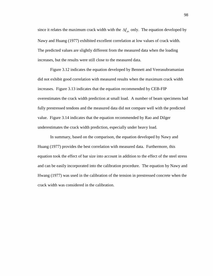
98
since it relates the maximum crack width with the psf only. The equation developed by
Nawy and Huang (1977) exhibited excellent correlation at low values of crack width.
The predicted values are slightly different from the measured data when the loading
increases, but the results were still close to the measured data.
Figure 3.12 indicates the equation developed by Bennett and Veerasubramanian
did not exhibit good correlation with measured results when the maximum crack width
increases. Figure 3.13 indicates that the equation recommended by CEB-FIP
overestimates the crack width prediction at small load. A number of beam specimens had
fully prestressed tendons and the measured data did not compare well with the predicted
value. Figure 3.14 indicates that the equation recommended by Rao and Dilger
underestimates the crack width prediction, especially under heavy load.
In summary, based on the comparison, the equation developed by Nawy and
Huang (1977) provides the best correlation with measured data. Furthermore, this
equation took the effect of bar size into account in addition to the effect of the steel stress
and can be easily incorporated into the calibration procedure. The equation by Nawy and
Hwang (1977) was used in the calibration of the tension in prestressed concrete when the
crack width was considered in the calibration.

99
Figure 3.11 Comparison of the measured and predicted maximum crack widths using
equations developed by Nawy and Huang (1977) and Nawy and Potyondy (1971).
Figure 3.12 Comparison of the measured and predicted maximum crack widths using
equations developed by Nawy and Huang (1977) and Bennett and Veerasubramanian
(1972).
0
0.01
0.02
0.03
0.04
0.05
0 0.01 0.02 0.03 0.04 0.05
Nawy and HuangNawy and PotyondyPerfect Correlation
Pre
dic
ted
Maxim
um
Cra
ck W
idth
(in
.)
Measured Maximum Crack Width (in.)
0
0.01
0.02
0.03
0.04
0.05
0 0.01 0.02 0.03 0.04 0.05
Nawy and HuangBennett and
VeerasubramanianPerfect Correlation
Pre
dic
ted
Maxim
um
Cra
ck W
idth
(in
.)
Measured Maximum Crack Width (in.)
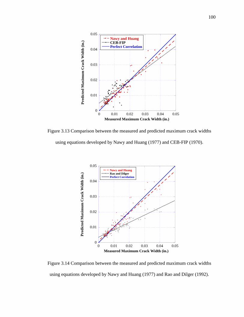
100
Figure 3.13 Comparison between the measured and predicted maximum crack widths
using equations developed by Nawy and Huang (1977) and CEB-FIP (1970).
Figure 3.14 Comparison between the measured and predicted maximum crack widths
using equations developed by Nawy and Huang (1977) and Rao and Dilger (1992).
0
0.01
0.02
0.03
0.04
0.05
0 0.01 0.02 0.03 0.04 0.05
Nawy and HuangCEB-FIPPerfect Correlation
Pre
dic
ted
Maxim
um
Cra
ck W
idth
(in
.)
Measured Maximum Crack Width (in.)
0
0.01
0.02
0.03
0.04
0.05
0 0.01 0.02 0.03 0.04 0.05
Nawy and Huang
Rao and Dilger
Perfect Correlation
Pre
dic
ted
Maxim
um
Cra
ck W
idth
(in
.)
Measured Maximum Crack Width (in.)
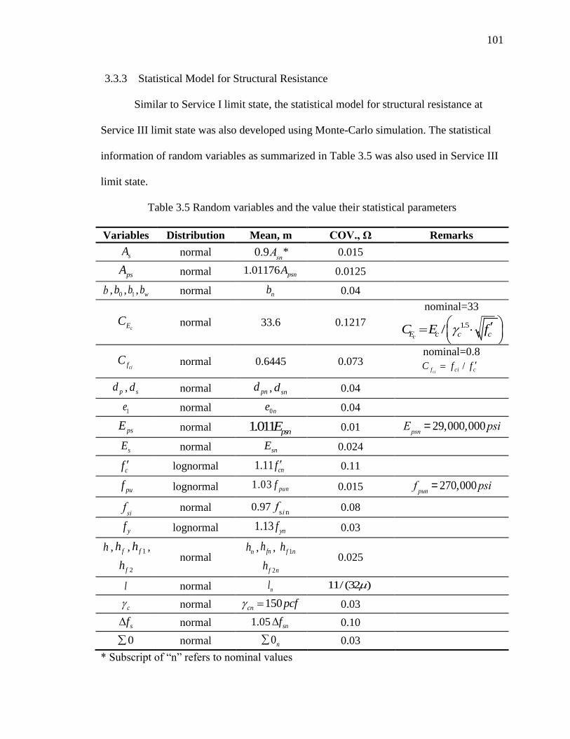
101
3.3.3 Statistical Model for Structural Resistance
Similar to Service I limit state, the statistical model for structural resistance at
Service III limit state was also developed using Monte-Carlo simulation. The statistical
information of random variables as summarized in Table 3.5 was also used in Service III
limit state.
Table 3.5 Random variables and the value their statistical parameters
Variables Distribution Mean, m COV., Ω Remarks
sA
normal 0.9Asn
* 0.015
psA
normal 1.01176 psnA 0.0125
b , 0b , 1b , wb normal nb 0.04
cEC
normal 33.6 0.1217
nominal=33
1.5/cE c c cC E f
cifC
normal 0.6445 0.073 nominal=0.8
/cif ci cC f f
pd , sd normal pnd , snd 0.04
1e normal 0ne 0.04
psE
normal 1.011 psnE 0.01 Epsn
= 29,000,000psi
sE normal snE
0.024
cf lognormal 1.11 cnf 0.11
puf
lognormal 1.03 punf 0.015 fpun
= 270,000psi
fsi
normal 0.97 fsi n
0.08
yf lognormal 1.13 ynf
0.03
h , fh , 1fh ,
2fh normal
nh , fnh , 1f nh
2f nh 0.025
l normal nl 11/(32 )
c normal 150cn pcf 0.03
sf normal 1.05 snf 0.10
0 normal 0n
0.03
* Subscript of “n” refers to nominal values
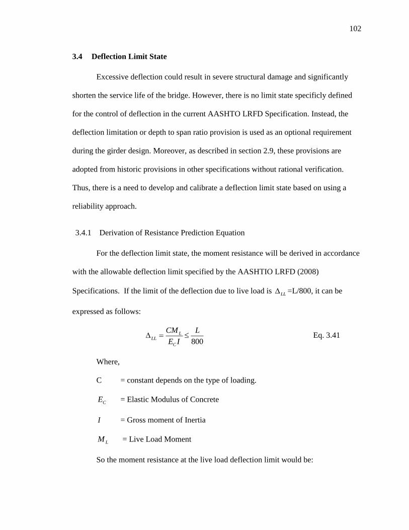
102
3.4 Deflection Limit State
Excessive deflection could result in severe structural damage and significantly
shorten the service life of the bridge. However, there is no limit state specificly defined
for the control of deflection in the current AASHTO LRFD Specification. Instead, the
deflection limitation or depth to span ratio provision is used as an optional requirement
during the girder design. Moreover, as described in section 2.9, these provisions are
adopted from historic provisions in other specifications without rational verification.
Thus, there is a need to develop and calibrate a deflection limit state based on using a
reliability approach.
3.4.1 Derivation of Resistance Prediction Equation
For the deflection limit state, the moment resistance will be derived in accordance
with the allowable deflection limit specified by the AASHTIO LRFD (2008)
Specifications. If the limit of the deflection due to live load is LL =L/800, it can be
expressed as follows:
800
LLL
C
CM L
E I Eq. 3.41
Where,
C = constant depends on the type of loading.
CE = Elastic Modulus of Concrete
I = Gross moment of Inertia
LM = Live Load Moment
So the moment resistance at the live load deflection limit would be:

103
.800
CL
E ILM
C Eq. 3.42
The total resistance moment at the limit state is given by,
.800
CALL D L D
E ILM M M M
C Eq. 3.43
Eq. 3.43 is applicable if the total resistance moment is less than the cracking
moment, crM . If the total resistance moment is larger than crM , Eq. 3.43 will need to be
re-adjusted to account for the cracked section behavior. The bilinear model for the
moment of inertia can be used and the resistance moment will be as follows:
. ( )[1 ]800
c e eALL D L cr D D
g
E I ILM M M M M M
C I Eq. 3.44
Where, eI is the effective moment of inertia that can be expressed in terms of the
cracking moment, total moment, and cracking moment of Inertia, crI . The cracking
moment of inertia, crI , is computed in terms of the depth of the neutral axis. The depth
of the neutral axis can be determined from equilibrium equations and strain compatibility.
Solving all equation simultaneously, the total resistance moment of the limit state of
immediate deflection will be formulated.
3.4.2 Statistical Model for Structural Resistance

104
Similar to the Service III limit state, the statistical model for structural resistance
was developed using Monte-Carlo simulation. The statistical information of random
variables that summarized in Table 3.5 will be also used in Deflection limit state.

105
4 MODELS FOR LIVE LOAD
CHAPTER 4
MODELS FOR LIVE LOAD
Live load models and their statistical characteristics are essential parts of any
structural reliability analysis. The prediction of the maximum load effect for various
durations is one of the most important steps in developing and calibrating the
serviceability limit states. During the calibration of strength limit states for AASHTO
LRFD Bridge Design Specifications. A new live load model, HL-93 developed based on
the Ontario truck survey data was adopted by AASHTO (Figure 4.1) (Nowak, 1999). In
addition to HL-93 live load model, AASHTO also specified that owner-specified special
design vehicles can be used in load combination for Strength II limit state, Figure 4.2
shows the permit vehicle specified in NJDOT Bridge Design Manual.
Figure 4.1 HL-93 Design Live Load Model (Nowak 1999)
8 kips 32 kips 32 kips
14 ft 14 ft ~ 30 ft
0.64 k/ft25 kips
or
25 kips
4 ft

106
Figure 4.2 NJDOT Design Permit Vehicle (NJDOT, 2010)
The load effect in terms of moment and shear can be determined by running each
truck over an influence line on various span lengths. The bias factor was calculated as a
ratio between the load effect due to each truck and the effect due to design live load
model. This factor was calculated for each Ontario truck and plotted on normal
probability paper (NPP). Then the bias factors were extrapolated to various time periods
at different span lengths. Table 4.1 presents the bias factors in terms of simple span
moments calculated by Nowak during the LRFD calibration.
In this section, WIM data collected from various states will be processed using
specially developed quality control and filtering routines to identify weighing errors,
unusual truck configurations, and permit loads. Various refined prediction techniques
will be used to extrapolate the load effects to various time periods. Moreover, live load
models are proposed for various limit states.

107
Table 4.1 Mean Maximum Moments for Simple Spans Divided by Corresponding HL-93
Moments (Nowak 1999)
Span
(ft)
M (HL-93)
(k-ft)
Duration
1
day
2
weeks
1
month
2
months
6
months
1
year
5
years
50
years
75
years
10 88 0.88 1.02 1.07 1.12 1.18 1.25 1.33 1.5 1.5
20 232 0.9 0.98 1.02 1.06 1.1 1.14 1.21 1.3 1.3
30 397 0.95 1.04 1.08 1.12 1.15 1.19 1.26 1.35 1.35
40 578 1.02 1.11 1.14 1.17 1.21 1.23 1.28 1.35 1.35
50 826 1 1.08 1.12 1.15 1.18 1.22 1.25 1.33 1.33
60 1093 1.02 1.09 1.12 1.15 1.18 1.21 1.24 1.32 1.32
70 1376 1.02 1.08 1.12 1.15 1.18 1.21 1.25 1.31 1.31
80 1675 1.02 1.08 1.11 1.14 1.17 1.21 1.25 1.32 1.32
90 1990 1.02 1.08 1.11 1.14 1.16 1.2 1.24 1.31 1.31
100 2322 1.02 1.08 1.1 1.13 1.16 1.2 1.24 1.31 1.31
110 2670 1.02 1.07 1.1 1.12 1.15 1.19 1.24 1.31 1.31
120 3033 1.01 1.07 1.09 1.12 1.15 1.18 1.22 1.29 1.29
130 3413 1 1.06 1.09 1.11 1.13 1.16 1.2 1.27 1.27
140 3809 0.98 1.03 1.06 1.08 1.1 1.13 1.17 1.24 1.24
150 4220 0.98 1.03 1.06 1.07 1.09 1.12 1.16 1.23 1.23
160 4648 0.98 1.03 1.07 1.09 1.1 1.13 1.17 1.24 1.24
170 5092 0.99 1.03 1.07 1.09 1.11 1.13 1.18 1.24 1.24
180 5552 0.98 1.03 1.06 1.08 1.11 1.13 1.17 1.24 1.24
190 6028 0.97 1.02 1.06 1.08 1.1 1.13 1.17 1.24 1.24
200 6520 0.96 1.02 1.05 1.08 1.09 1.12 1.16 1.23 1.23
4.1 Analysis of Live Load Data
4.1.1 WIM Data Processing
Truck data from each WIM site was processed using the filtering criteria are listed
below and Table 4.2 presents the number and percentage of trucks filtered by various
filters. It is observed that the filter criteria 1 (minimum gross vehicle weight (GVW) of
at least 15 kips) filters the most number of vehicles, ranging from 2.2% to 13.0%. This
criterion removes any inconsequential truck records, passenger vehicles misclassified as

108
trucks, and sensor errors in measuring light axles. For the qualified trucks, the
percentage range from 81.8% to 91.5%.
Filter Description
1. Gross Wt < 15k
2. Omit Class = 15
3. Tandems > 60k
4. Num of Axles=9 & Gross Wt>150k
5. Class = 9 & Wt1 > 15k
6. Class 8, if S3>5ft and GVW<20k
7. Num of Axles=10 & Gross Wt>200k
8. Any single axle over 40k
9. No axle spaces less than 2.5ft
10. 3 or more tandems = Permit
11. Permitted Cranes
12. Permitted Cranes with First Spacing<8.5ft, L<50ft, W>100k
13. Find and Reassign Fake CL13, split to CL9 + CL2
14. Find if L>50ft and GVW<20k, possible cars lumped together
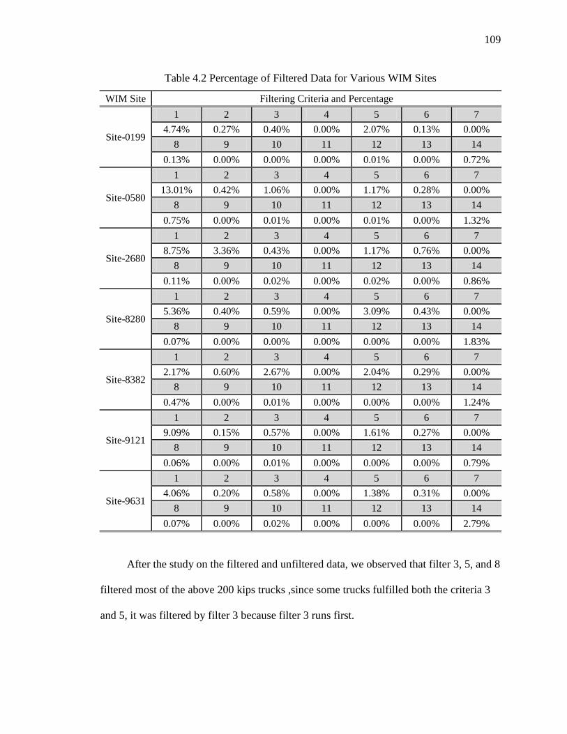
109
Table 4.2 Percentage of Filtered Data for Various WIM Sites
WIM Site Filtering Criteria and Percentage
Site-0199
1 2 3 4 5 6 7
4.74% 0.27% 0.40% 0.00% 2.07% 0.13% 0.00%
8 9 10 11 12 13 14
0.13% 0.00% 0.00% 0.00% 0.01% 0.00% 0.72%
Site-0580
1 2 3 4 5 6 7
13.01% 0.42% 1.06% 0.00% 1.17% 0.28% 0.00%
8 9 10 11 12 13 14
0.75% 0.00% 0.01% 0.00% 0.01% 0.00% 1.32%
Site-2680
1 2 3 4 5 6 7
8.75% 3.36% 0.43% 0.00% 1.17% 0.76% 0.00%
8 9 10 11 12 13 14
0.11% 0.00% 0.02% 0.00% 0.02% 0.00% 0.86%
Site-8280
1 2 3 4 5 6 7
5.36% 0.40% 0.59% 0.00% 3.09% 0.43% 0.00%
8 9 10 11 12 13 14
0.07% 0.00% 0.00% 0.00% 0.00% 0.00% 1.83%
Site-8382
1 2 3 4 5 6 7
2.17% 0.60% 2.67% 0.00% 2.04% 0.29% 0.00%
8 9 10 11 12 13 14
0.47% 0.00% 0.01% 0.00% 0.00% 0.00% 1.24%
Site-9121
1 2 3 4 5 6 7
9.09% 0.15% 0.57% 0.00% 1.61% 0.27% 0.00%
8 9 10 11 12 13 14
0.06% 0.00% 0.01% 0.00% 0.00% 0.00% 0.79%
Site-9631
1 2 3 4 5 6 7
4.06% 0.20% 0.58% 0.00% 1.38% 0.31% 0.00%
8 9 10 11 12 13 14
0.07% 0.00% 0.02% 0.00% 0.00% 0.00% 2.79%
After the study on the filtered and unfiltered data, we observed that filter 3, 5, and 8
filtered most of the above 200 kips trucks ,since some trucks fulfilled both the criteria 3
and 5, it was filtered by filter 3 because filter 3 runs first.

110
4.1.2 Statistics of WIM data
The following GVW study is based on the New York and Florida WIM data
which was processed by the processing program shown in section 4.1.1. Figure 4.3
through Figure 4.11 present the histogram and statistics results of all the NY sites. Figure
4.12 and Figure 4.13 show the histogram and statistics of Florida sites.
Figure 4.3 Histogram of Site 0199-South Bound
Figure 4.4 Histogram of Site 0199-North Bound
0%
5%
10%
15%
20%
25%
30%
19.20%
26.55%
16.01%
9.23%
6.98% 6.53%
4.41%
2.21%
0.94%0.41% 0.14% 0.04% 0.01% 0.00% 0.00% 0.00% 0.00% 0.00% 0.00% 0.00% 0.00%
Percen
tage (%
)
GVW (kips)
Site 0199-South Bound
Total Weight Histogram
N=585084
Class Count AVGWt StDev MaxWt
1 0 0 0 0
2 2554 0 0 0
3 0 0 0 0
4 8491 40 13.81 104.3
5 89670 24.33 9.34 130.8
6 45949 36.2 16.69 112.9
7 28250 51.33 23.39 143
8 54089 40.29 13.64 148.8
9 326149 50.14 20.32 147.9
10 10705 72.46 27.64 168.1
11 17707 51.98 17.77 164.8
12 4074 57.76 20.77 179.3
13 0 0 0 0
14 0 0 0 0
15 0 0 0 0
Site 0199-South Bound
0%
2%
4%
6%
8%
10%
12%
14%
16%
18%
13.19%
17.08%
16.21%
11.54%10.91%
14.49%
6.33%
1.41%0.51%
0.23%0.10%0.03%0.01%0.00%0.00% 0.00%0.00% 0.00%0.00%0.00%0.00%
Percen
tag
e (%
)
GVW (kips)
Site 0199-North Bound
Total Weight Histogram
N=1801752
Class Count AVGWt StDev MaxWt
1 0 0 0 0
2 4468 0 0 0
3 0 0 0 0
4 30140 39.39 10.78 94.4
5 318693 22.63 6.35 126.7
6 122431 35.07 12.42 115.3
7 17361 71.13 19.57 144.2
8 172500 40.92 10.37 130.6
9 1092059 60.15 17.71 144
10 11140 90.16 30.35 161.7
11 28856 58.05 11.79 158.8
12 8572 62.64 14.91 169.7
13 0 0 0 0
14 0 0 0 0
15 0 0 0 0
Site 0199-North Bound

111
Figure 4.5 Histogram of Site 0580-East Bound
Figure 4.6 Histogram of Site 0580-West Bound
0%
5%
10%
15%
20%
25%
21.63%
20.49%
14.25%
7.44%
5.17% 5.48%
3.82%
1.98% 1.91% 1.92%1.28%
0.56% 0.16% 0.03% 0.00% 0.00% 0.00% 0.00% 0.00% 0.00% 0.00%
Percen
tage (%
)
GVW (kips)
Site 0580-East Bound
Total Weight Histogram
N=1337827
Class Count AVGWt StDev MaxWt
1 0 0 0 0
2 8054 0 0 0
3 0 0 0 0
4 75362 38.82 10.79 103
5 442108 23.5 7.2 137
6 157319 39.92 15.3 117.9
7 12443 63.71 22.38 148.9
8 107146 39.3 11.81 149.8
9 429203 56.1 20.08 141.5
10 100109 104.36 24.99 171.6
11 9927 53.63 14.05 155.1
12 4210 64.32 15.66 190.3
13 0 0 0 0
14 0 0 0 0
15 0 0 0 0
Site 0580-East Bound
0%
5%
10%
15%
20%
25%
22.25%
23.56%
15.44%
7.40%
4.08%3.40%
2.71%
1.36% 1.15%1.57% 1.35%
0.55%0.13% 0.03% 0.00% 0.00% 0.00% 0.00% 0.00% 0.00% 0.00%
Percen
tage (%
)
GVW (kips)
Site 0580-West Bound
Total Weight Histogram
N=1100501
Class Count AVGWt StDev MaxWt
1 0 0 0 0
2 8924 0 0 0
3 0 0 0 0
4 64307 38.66 10.48 105.8
5 399522 24.08 8.34 133.1
6 130282 41.44 16.46 117.9
7 13124 66.06 23.79 152.2
8 95222 40.82 13.74 145.1
9 324006 51.01 18.94 146.6
10 60087 107.04 27.2 213.4
11 8821 53.64 18.78 169.9
12 5130 51.29 20.76 177.8
13 0 0 0 0
14 0 0 0 0
15 0 0 0 0
Site 0580-West Bound

112
Figure 4.7 Histogram of Site 2680
Figure 4.8 Histogram of Site 8280
0%
5%
10%
15%
20%
25%
20.68%21.22%
13.16%
6.94%6.09%
6.72%
5.28%
3.16%
2.07%1.15%
0.56% 0.21% 0.07% 0.03% 0.01% 0.00% 0.00% 0.00% 0.00% 0.00% 0.00%
Percen
tag
e (%
)
GVW (kips)
Site 2680
Total Weight Histogram
N=122109
Class Count AVGWt StDev MaxWt
1 0 0 0 0
2 2200 0 0 0
3 0 0 0 0
4 721 34.75 11.02 71.9
5 28651 22.81 6.47 91.5
6 16716 36.13 14.51 113.6
7 7300 65.2 23.65 143.2
8 7553 37.18 11.63 125.9
9 47924 56.35 21.61 134.2
10 8798 78.98 33.82 174
11 2513 25.78 12.5 109.9
12 1933 31.03 19.06 153.6
13 0 0 0 0
14 0 0 0 0
15 0 0 0 0
Site 2680
0%
5%
10%
15%
20%
25%
9.85%
22.09%
17.37%
13.18% 13.07%13.31%
4.82%
1.12%0.55% 0.40% 0.26% 0.11% 0.03% 0.01% 0.00% 0.00% 0.00% 0.00% 0.00% 0.00% 0.00%
Percen
tag
e (%
)
GVW (kips)
Site 8280
Total Weight Histogram
N=1639135
Class Count AVGWt StDev MaxWt
1 0 0 0 0
2 16020 0 0 0
3 0 0 0 0
4 28408 29.21 11.34 101
5 85989 21.78 6.43 108.9
6 49021 30.64 12.56 116.8
7 8225 50.23 24.92 146.4
8 106679 36.68 11.33 152.8
9 1199676 54.42 17.79 142.3
10 30917 90.18 30.45 186.3
11 101404 54 15.62 169.3
12 28816 59.45 17.38 211.6
13 0 0 0 0
14 0 0 0 0
15 0 0 0 0
Site 8280
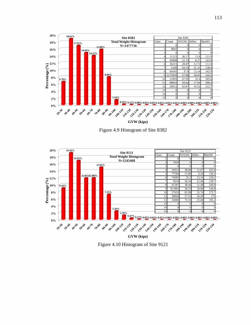
113
Figure 4.9 Histogram of Site 8382
Figure 4.10 Histogram of Site 9121
0%
2%
4%
6%
8%
10%
12%
14%
16%
18%
20%
6.70%
18.91%
17.01%
14.94%
14.11%
15.88%
8.04%
1.54%
0.26% 0.12% 0.08% 0.05% 0.03% 0.02% 0.01% 0.01% 0.00% 0.00% 0.00% 0.00% 0.00%
Percen
tag
e (%
)
GVW (kips)
Site 8382
Total Weight Histogram
N=1477736
Class Count AVGWt StDev MaxWt
1 0 0 0 0
2 9602 0 0 0
3 0 0 0 0
4 11115 36.17 11.8 111.9
5 45898 22.74 8.37 143.8
6 36215 28.87 12.72 111.9
7 5189 44.19 21.31 138.9
8 64545 37.9 13.14 142.9
9 1173959 57.08 18.05 144.5
10 12993 67.95 25.4 185.8
11 98810 59.64 17.04 188.4
12 29012 62.87 19.52 212.7
13 0 0 0 0
14 0 0 0 0
15 0 0 0 0
Site 8382
0%
2%
4%
6%
8%
10%
12%
14%
16%
18%
20%
9.10%
19.16%
16.93%
11.95%12.00%
15.02%
7.25%
2.50%
1.29%0.47%
0.13% 0.05% 0.02% 0.01% 0.00% 0.00% 0.00% 0.00% 0.00% 0.00% 0.00%
Percen
tage (%
)
GVW (kips)
Site 9121
Total Weight Histogram
N=1245468
Class Count AVGWt StDev MaxWt
1 0 0 0 0
2 7610 0 0 0
3 0 0 0 0
4 34313 38.06 11.07 101.6
5 77584 21.86 6.24 136.3
6 74391 31.2 12.14 119.1
7 8254 56.34 21.46 139.7
8 67287 38.46 11.48 140.9
9 911881 58.53 18.84 144.8
10 27633 82.99 25.76 175.7
11 28056 57.53 16.29 175
12 16069 73.33 25.48 191.2
13 0 0 0 0
14 0 0 0 0
15 0 0 0 0
Site 9121

114
Figure 4.11 Histogram of Site 9631
Figure 4.12 Histogram of Florida Site 9919
0%
5%
10%
15%
20%
25%
30%
11.77%
29.78%
14.71%
7.40%6.71% 6.93%
5.50% 5.33%
4.02%
1.80%0.58% 0.13% 0.03% 0.01% 0.00% 0.00% 0.00% 0.00% 0.00% 0.00% 0.00%
Percen
tage (%
)
GVW (kips)
Site 9631
Total Weight Histogram
N=246494Class Count AVGWt StDev MaxWt
1 0 0 0 0
2 1708 0 0 0
3 0 0 0 0
4 10832 36.91 11.43 109.9
5 20362 21.92 6.6 110.9
6 10122 33.28 13.5 108
7 1506 57.46 22.28 140.3
8 14404 37.5 9.64 132.9
9 172664 55.3 24.36 146.9
10 11745 88.93 26.52 176.2
11 3402 51.06 15.57 171.2
12 1457 89.55 26.05 160.9
13 0 0 0 0
14 0 0 0 0
15 0 0 0 0
Site 9631
0.00%
5.00%
10.00%
15.00%
20.00%
25.00%
6.33%
15.57%
23.85%
17.65% 17.96%
14.52%
3.79%
0.31%0.02%0.01%0.00%0.00%0.00%0.00%0.00%0.00%0.00%0.00%0.00%
Percen
tag
e (
%)
GVW (kips)
Florida Site 9919
Total Weight Histogram
Count Class AVGWt StDev MaxWt
0 1 0 0 0
0 2 0 0 0
0 3 0 0 0
13954 4 30.62 8 58.55
69914 5 19.31 3.37 62.56
36037 6 26.54 8.54 72.78
6387 7 53.94 8.15 81.59
52377 8 31.53 7.85 81.17
844762 9 47.25 14.21 103.28
7519 10 53.5 17.44 114.56
30728 11 49.68 10.11 84.79
9977 12 47.58 10.84 87.73
0 13 0 0 0
0 14 0 0 0
0 15 0 0 0
Florida Site 9919

115
Figure 4.13 Histogram of Florida Site 9927
4.1.3 Multiple Presence Probabilities
Multiple presence statistics are needed to estimate the maximum moment caused
by the presence of more than one truck on the bridge. Trucks may simultaneously occur
on a bridge in many different arrangements. In general, four truck loading patterns are
considered (see Figure 4.14):
(a) Single event; only one truck travels on the bridge span without any other trucks
following or on other lanes.
(b) Following or in-lane; two trucks following each other with a varying headway
distance measured from rear axle of one truck to front axle of the following truck
(c) Side-by-side in tandem; two trucks in adjacent lanes and overlapping by at least
one-half the body length of the leading truck
(d) Side-by-side but staggered; two trucks in adjacent lanes and overlapping by less
than at least one-half the body length of the leading truck
0.00%
5.00%
10.00%
15.00%
20.00%
25.00%
30.00%
18.03%
19.90%
28.65%
10.35%
5.56%6.34%
9.28%
1.85%
0.05%0.00%0.00%0.00%0.00%0.00%0.00%0.00%0.00%0.00%0.00%
Percen
tag
e (
%)
GVW (kips)
Florida Site 9927
Total Weight Histogram
Count Class AVGWt StDev MaxWt
0 1 0 0 0
10076 2 0 0 0
0 3 0 0 0
3254 4 33.19 9.73 64.21
21422 5 19.87 4.1 98.33
33583 6 24.24 8.95 98.89
3429 7 47.76 16.97 86.2
22693 8 35.91 12.03 91.88
136577 9 44.77 18.97 99.43
1604 10 55.17 21.76 99.14
1212 11 52.07 14.75 81.31
168 12 52.22 13.65 76.5
0 13 0 0 0
0 14 0 0 0
0 15 0 0 0
Florida Site 9927

116
Figure 4.14 Multiple Presence Categories
Truck loading, including weight and loading patterns, is generally site-specific.
Multiple presence statistics depend on factors such as truck volume, bridge span length,
local industry, law enforcement, and traffic flow control. This has also been recognized
by the AASHTO LRFD Specifications, which, despite having a calibrated live load
model, highlights consideration to site-specific modifications to design live loads for
cases in which the legal load is significantly greater than typical, there is an unusually
high percentage of truck traffic, or there is truck pooling. Therefore, it is important to
account for the uncertainty due to site variation in statistical modeling. Table 4.3 through
Table 4.12 summarized the multiple presence statistics extracted from WIM data from
various WIM sites. It shows that the percentage of following, side by side, and staggered
events increased when the span length increased.

117
Table 4.3 Summary of Multiple Presence Statistics (Newark Bay Bridge WIM Site)
Span Following Side by Side Staggered Single Other
40 0.01% 0.09% 0.00% 99.63% 0.27%
60 0.01% 0.43% 0.00% 99.29% 0.27%
80 0.01% 1.24% 0.03% 98.44% 0.28%
100 0.02% 2.42% 0.21% 97.06% 0.30%
120 0.04% 3.30% 1.02% 95.30% 0.34%
140 0.12% 3.70% 2.49% 93.27% 0.42%
160 0.43% 3.80% 4.28% 90.93% 0.56%
180 1.24% 3.77% 6.11% 88.04% 0.84%
200 2.75% 3.68% 7.70% 84.55% 1.33%
Table 4.4 Summary of Multiple Presence Statistics (NY WIM Site 2680)
Span Following Side by Side Staggered Single Other
40 0.39% 0.06% 0.01% 95.44% 4.10%
60 0.39% 0.09% 0.03% 95.32% 4.17%
80 0.39% 0.16% 0.07% 95.11% 4.27%
100 0.41% 0.19% 0.14% 94.91% 4.35%
120 0.44% 0.19% 0.21% 94.72% 4.44%
140 0.51% 0.19% 0.28% 94.49% 4.53%
160 0.60% 0.19% 0.35% 94.21% 4.65%
180 0.73% 0.19% 0.43% 93.90% 4.75%
200 0.88% 0.18% 0.48% 93.60% 4.86%
Table 4.5 Summary of Multiple Presence Statistics (NY WIM Site 0199-I95)
Span Following Side by Side Staggered Single Other
40 0.01% 0.12% 0.00% 99.63% 0.24%
60 0.01% 0.47% 0.00% 99.25% 0.27%
80 0.01% 1.21% 0.03% 98.41% 0.34%
100 0.01% 2.21% 0.27% 97.07% 0.44%
120 0.03% 2.86% 1.21% 95.36% 0.54%
140 0.14% 3.06% 2.65% 93.44% 0.71%
160 0.49% 3.04% 4.29% 91.30% 0.88%
180 1.54% 2.99% 5.92% 88.43% 1.12%
200 3.63% 2.90% 7.39% 84.55% 1.53%
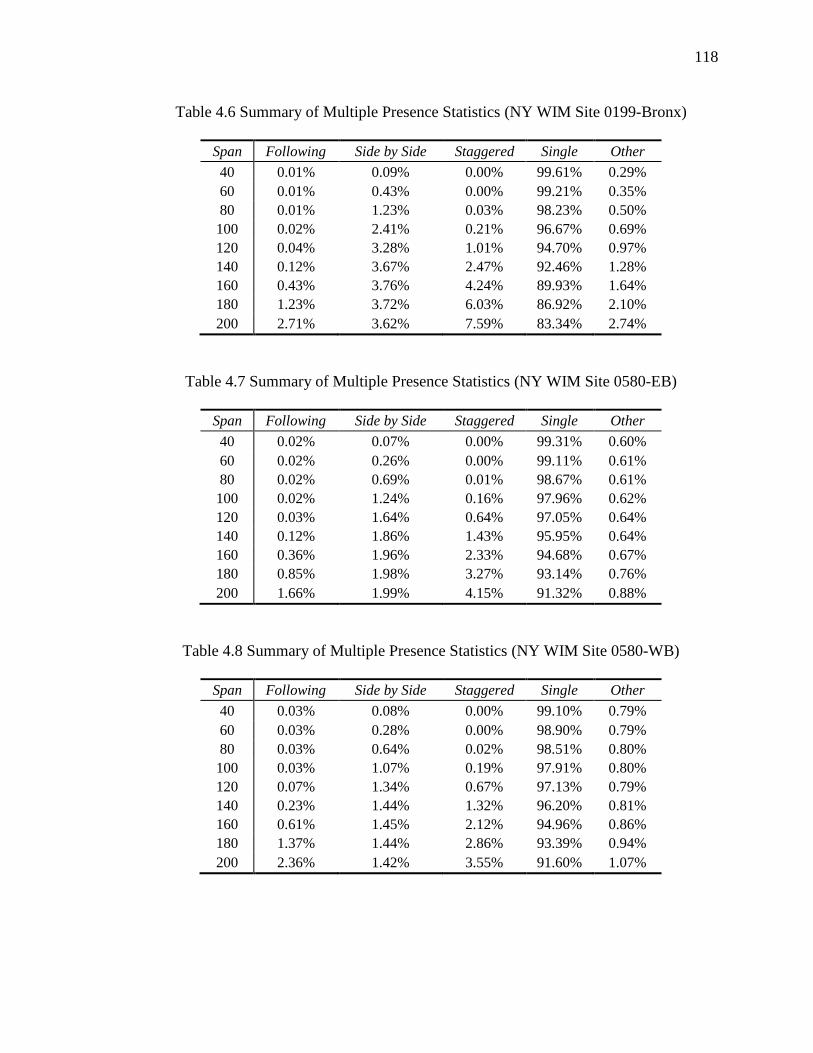
118
Table 4.6 Summary of Multiple Presence Statistics (NY WIM Site 0199-Bronx)
Span Following Side by Side Staggered Single Other
40 0.01% 0.09% 0.00% 99.61% 0.29%
60 0.01% 0.43% 0.00% 99.21% 0.35%
80 0.01% 1.23% 0.03% 98.23% 0.50%
100 0.02% 2.41% 0.21% 96.67% 0.69%
120 0.04% 3.28% 1.01% 94.70% 0.97%
140 0.12% 3.67% 2.47% 92.46% 1.28%
160 0.43% 3.76% 4.24% 89.93% 1.64%
180 1.23% 3.72% 6.03% 86.92% 2.10%
200 2.71% 3.62% 7.59% 83.34% 2.74%
Table 4.7 Summary of Multiple Presence Statistics (NY WIM Site 0580-EB)
Span Following Side by Side Staggered Single Other
40 0.02% 0.07% 0.00% 99.31% 0.60%
60 0.02% 0.26% 0.00% 99.11% 0.61%
80 0.02% 0.69% 0.01% 98.67% 0.61%
100 0.02% 1.24% 0.16% 97.96% 0.62%
120 0.03% 1.64% 0.64% 97.05% 0.64%
140 0.12% 1.86% 1.43% 95.95% 0.64%
160 0.36% 1.96% 2.33% 94.68% 0.67%
180 0.85% 1.98% 3.27% 93.14% 0.76%
200 1.66% 1.99% 4.15% 91.32% 0.88%
Table 4.8 Summary of Multiple Presence Statistics (NY WIM Site 0580-WB)
Span Following Side by Side Staggered Single Other
40 0.03% 0.08% 0.00% 99.10% 0.79%
60 0.03% 0.28% 0.00% 98.90% 0.79%
80 0.03% 0.64% 0.02% 98.51% 0.80%
100 0.03% 1.07% 0.19% 97.91% 0.80%
120 0.07% 1.34% 0.67% 97.13% 0.79%
140 0.23% 1.44% 1.32% 96.20% 0.81%
160 0.61% 1.45% 2.12% 94.96% 0.86%
180 1.37% 1.44% 2.86% 93.39% 0.94%
200 2.36% 1.42% 3.55% 91.60% 1.07%
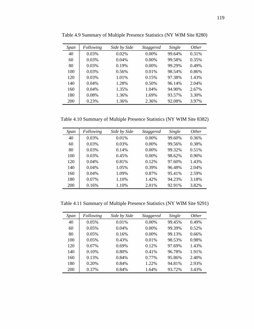
119
Table 4.9 Summary of Multiple Presence Statistics (NY WIM Site 8280)
Span Following Side by Side Staggered Single Other
40 0.03% 0.02% 0.00% 99.64% 0.31%
60 0.03% 0.04% 0.00% 99.58% 0.35%
80 0.03% 0.19% 0.00% 99.29% 0.49%
100 0.03% 0.56% 0.01% 98.54% 0.86%
120 0.03% 1.01% 0.15% 97.38% 1.43%
140 0.04% 1.28% 0.50% 96.14% 2.04%
160 0.04% 1.35% 1.04% 94.90% 2.67%
180 0.08% 1.36% 1.69% 93.57% 3.30%
200 0.23% 1.36% 2.36% 92.08% 3.97%
Table 4.10 Summary of Multiple Presence Statistics (NY WIM Site 8382)
Span Following Side by Side Staggered Single Other
40 0.03% 0.01% 0.00% 99.60% 0.36%
60 0.03% 0.03% 0.00% 99.56% 0.38%
80 0.03% 0.14% 0.00% 99.32% 0.51%
100 0.03% 0.45% 0.00% 98.62% 0.90%
120 0.04% 0.81% 0.12% 97.60% 1.43%
140 0.04% 1.05% 0.39% 96.48% 2.04%
160 0.04% 1.09% 0.87% 95.41% 2.59%
180 0.07% 1.10% 1.42% 94.23% 3.18%
200 0.16% 1.10% 2.01% 92.91% 3.82%
Table 4.11 Summary of Multiple Presence Statistics (NY WIM Site 9291)
Span Following Side by Side Staggered Single Other
40 0.05% 0.01% 0.00% 99.45% 0.49%
60 0.05% 0.04% 0.00% 99.39% 0.52%
80 0.05% 0.16% 0.00% 99.13% 0.66%
100 0.05% 0.43% 0.01% 98.53% 0.98%
120 0.07% 0.69% 0.12% 97.69% 1.43%
140 0.10% 0.80% 0.41% 96.78% 1.91%
160 0.13% 0.84% 0.77% 95.86% 2.40%
180 0.20% 0.84% 1.22% 94.81% 2.93%
200 0.37% 0.84% 1.64% 93.72% 3.43%

120
Table 4.12 Summary of Multiple Presence Statistics (NY WIM Site 9631)
Span Following Side by Side Staggered Single Other
40 0.21% 0.02% 0.00% 97.90% 1.87%
60 0.21% 0.03% 0.00% 97.89% 1.87%
80 0.21% 0.08% 0.00% 97.80% 1.91%
100 0.21% 0.17% 0.00% 97.61% 2.01%
120 0.21% 0.23% 0.02% 97.40% 2.14%
140 0.21% 0.25% 0.08% 97.18% 2.28%
160 0.21% 0.26% 0.17% 96.96% 2.40%
180 0.23% 0.26% 0.25% 96.70% 2.56%
200 0.28% 0.26% 0.34% 96.40% 2.72%
4.2 Prediction of Long Term Live Load Effects
The prediction of the long term load effect is one of the most important steps in
performing structural analysis. During the AASHTO LRFD calibration process, a 1975
truck weight survey from Ontario, Canada, performed by the Ontario Ministry of
Transportation, was used (Agarwal and Wolkowicz, 1976). The survey included about
10,000 trucks that were randomly selected and stopped if they appeared to be heavy. If
the weight of the truck was heavy in comparison to the average weight in its category, the
truck record was retained; otherwise, the truck record was dismissed and not included in
the dataset. Assuming this dataset to represent the upper 20% of 2 weeks of normal truck
traffic in the United States (this corresponds to ADTT = 5000). In the original LRFD
code calibration by Nowak (1994), extrapolation was done by simple linear extension of
the upper tail to desired future level. In this section, various methods of predicting long
term load effects were discussed including methods based on rate of increase in vehicle
weight and probabilitic based extrapolation methods. The long term load effects from
various sites predicted using various methods were also discussed in this section.
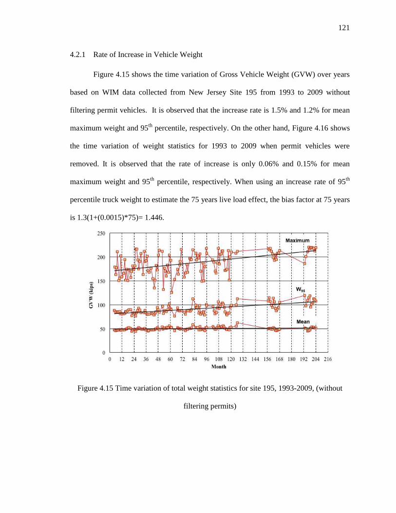
121
4.2.1 Rate of Increase in Vehicle Weight
Figure 4.15 shows the time variation of Gross Vehicle Weight (GVW) over years
based on WIM data collected from New Jersey Site 195 from 1993 to 2009 without
filtering permit vehicles. It is observed that the increase rate is 1.5% and 1.2% for mean
maximum weight and 95th
percentile, respectively. On the other hand, Figure 4.16 shows
the time variation of weight statistics for 1993 to 2009 when permit vehicles were
removed. It is observed that the rate of increase is only 0.06% and 0.15% for mean
maximum weight and 95th
percentile, respectively. When using an increase rate of 95th
percentile truck weight to estimate the 75 years live load effect, the bias factor at 75 years
is 1.3(1+(0.0015)*75)= 1.446.
Figure 4.15 Time variation of total weight statistics for site 195, 1993-2009, (without
filtering permits)
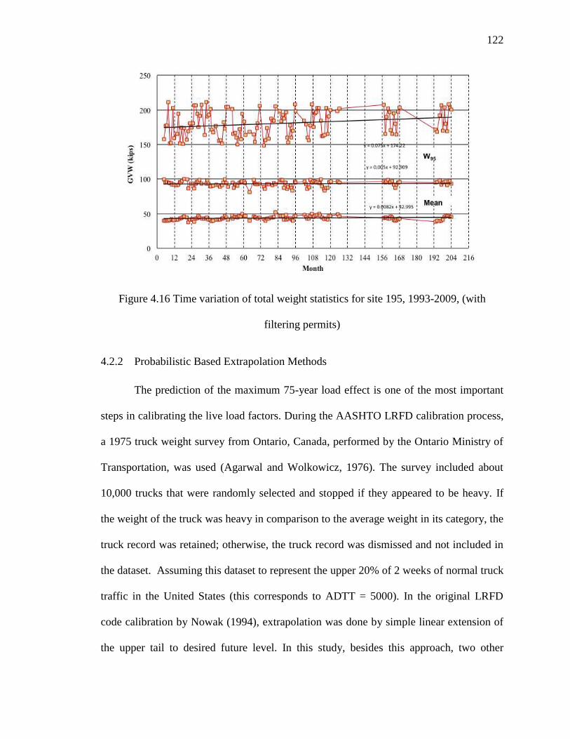
122
Figure 4.16 Time variation of total weight statistics for site 195, 1993-2009, (with
filtering permits)
4.2.2 Probabilistic Based Extrapolation Methods
The prediction of the maximum 75-year load effect is one of the most important
steps in calibrating the live load factors. During the AASHTO LRFD calibration process,
a 1975 truck weight survey from Ontario, Canada, performed by the Ontario Ministry of
Transportation, was used (Agarwal and Wolkowicz, 1976). The survey included about
10,000 trucks that were randomly selected and stopped if they appeared to be heavy. If
the weight of the truck was heavy in comparison to the average weight in its category, the
truck record was retained; otherwise, the truck record was dismissed and not included in
the dataset. Assuming this dataset to represent the upper 20% of 2 weeks of normal truck
traffic in the United States (this corresponds to ADTT = 5000). In the original LRFD
code calibration by Nowak (1994), extrapolation was done by simple linear extension of
the upper tail to desired future level. In this study, besides this approach, two other

123
approaches were also used in this study. Each approach is briefly discussed in the
following section.
a. Linear extension approach, the following steps were followed: (1) Calculate the
moment ratio due to every truck from WIM data using the computer program
developed by the authors; (2) Plot the calculation ratios on the Normal Probability
Paper; (3) Extend the upper tail (20% of the total number of trucks by weight) as a
straight-line to the desired future level. The x-coordinate of the intersection
between the extension line and the 75-year level line is the bias factor
representing the maximum 75-year load effects.
b. Re-plotting the upper tail using normal approximation with mean and standard
deviation of upper tail data, the following steps were used: (1) Calculate the
moment ratio due to every truck from WIM data using the computer program
developed by the authors; (2) Re-plot the upper tail points on the Normal
Probability paper with the best-fit normal distribution; (3) Extrapolate the
resulting normal distribution to the desired future level. The x-coordinate of the
intersection between the extension line and 75-year level is the bias factor
representing the maximum 75-year load effects.
c. Re-plotting the upper tail using best-fit straight line in data points, the following
steps were followed: (1) Calculate the moment ratio due to every truck from WIM
data using the computer program developed by the authors; (2) Re-plot the upper
tail points on the Normal Probability paper; (3) extrapolate the upper tail points as
a best-fit straight line to the desired future level. The x-coordinate of the
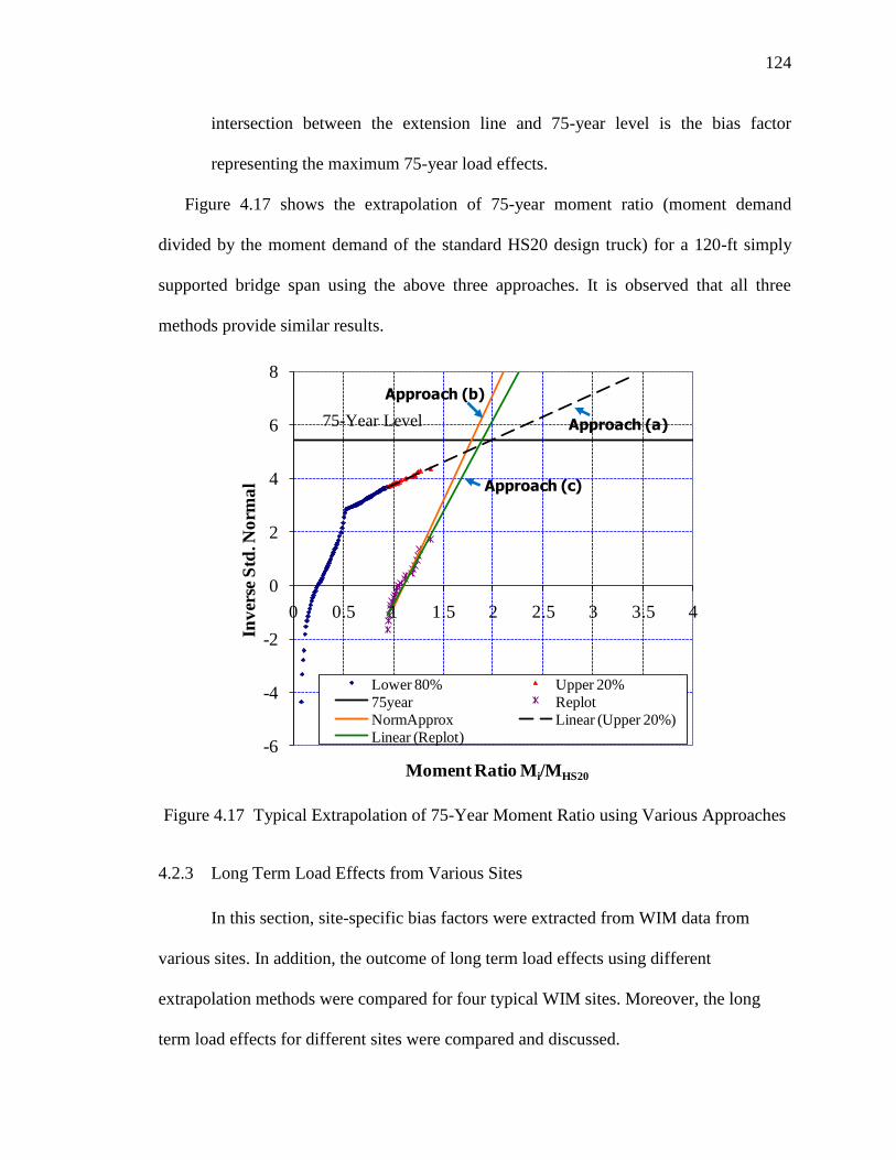
124
intersection between the extension line and 75-year level is the bias factor
representing the maximum 75-year load effects.
Figure 4.17 shows the extrapolation of 75-year moment ratio (moment demand
divided by the moment demand of the standard HS20 design truck) for a 120-ft simply
supported bridge span using the above three approaches. It is observed that all three
methods provide similar results.
Figure 4.17 Typical Extrapolation of 75-Year Moment Ratio using Various Approaches
4.2.3 Long Term Load Effects from Various Sites
In this section, site-specific bias factors were extracted from WIM data from
various sites. In addition, the outcome of long term load effects using different
extrapolation methods were compared for four typical WIM sites. Moreover, the long
term load effects for different sites were compared and discussed.
-6
-4
-2
0
2
4
6
8
0 0.5 1 1.5 2 2.5 3 3.5 4
Inv
erse
Std
. No
rma
l
Moment Ratio Mi/MHS20
Lower 80% Upper 20%
75year Replot
NormApprox Linear (Upper 20%)
Linear (Replot)
75-Year Level Approach (a)
Approach (c)
Approach (b)

125
4.2.3.1 Site-Specific Bias Factors for Various WIM Sites
Table 4.13 through Table 4.20 present the bias factors for eight New York WIM
sites that obtained using up 20% extrapolation. In addition, Table 4.21 presents the bias
factors for New Jersey WIM site that also obtained using up 20% extrapolation. The NJ
data was collected by Rutgers team at the Newark Bay Bridge site on NJ Turnpike. The
Newark Bay Bridge connects the Newark and Bayonne with truck traffic between
Newark and New York City. Since the NJ and NY are two neighboring states, the
comparison of long term live load effect between NJ and NY could help to better
understand the live load in this region and exam the consistency of the data. All the
moment ratios in this section are shown in terms of HL-93 loading.
Table 4.13 Mean Maximum Moments for Simple Spans Divided by Corresponding HL-
93 Moment for site NY0199-NB
Span
(ft) 1 day
2
weeks
1
month
2
months
6
months
1
year
5
years
50
years
75
years
20 1.343 1.525 1.572 1.615 1.679 1.719 1.807 1.925 1.944
40 1.334 1.511 1.558 1.599 1.662 1.701 1.787 1.902 1.921
60 1.236 1.379 1.417 1.451 1.501 1.533 1.602 1.694 1.710
80 1.187 1.312 1.344 1.374 1.417 1.445 1.505 1.585 1.599
100 1.143 1.260 1.291 1.319 1.361 1.386 1.443 1.519 1.532
120 1.097 1.209 1.238 1.264 1.304 1.329 1.382 1.454 1.467
140 1.054 1.160 1.188 1.212 1.250 1.273 1.324 1.392 1.404
160 1.011 1.112 1.139 1.163 1.199 1.221 1.270 1.336 1.348
180 0.969 1.067 1.093 1.116 1.151 1.172 1.219 1.283 1.294
200 0.931 1.024 1.050 1.071 1.104 1.125 1.170 1.230 1.240
220 0.894 0.986 1.011 1.033 1.065 1.086 1.131 1.191 1.201
240 0.862 0.949 0.973 0.993 1.025 1.044 1.087 1.143 1.153
260 0.830 0.915 0.938 0.958 0.989 1.007 1.048 1.103 1.113
280 0.801 0.883 0.905 0.924 0.954 0.972 1.012 1.066 1.075
300 0.774 0.854 0.875 0.893 0.922 0.940 0.978 1.029 1.038

126
Table 4.14 Mean Maximum Moments for Simple Spans Divided by Corresponding HL-
93 Moment for Site NY0199-SB
Span
(ft) 1 day
2
weeks
1
month
2
months
6
months
1
year
5
years
50
years
75
years
20 1.470 1.672 1.726 1.772 1.844 1.888 1.984 2.113 2.135
40 1.464 1.653 1.703 1.746 1.812 1.854 1.944 2.065 2.086
60 1.314 1.469 1.510 1.546 1.600 1.634 1.709 1.808 1.825
80 1.225 1.368 1.406 1.439 1.490 1.521 1.590 1.682 1.697
100 1.156 1.292 1.328 1.359 1.407 1.437 1.502 1.589 1.604
120 1.099 1.227 1.261 1.291 1.336 1.364 1.425 1.507 1.521
140 1.048 1.172 1.204 1.233 1.276 1.303 1.362 1.441 1.454
160 1.002 1.121 1.152 1.180 1.223 1.249 1.306 1.383 1.395
180 0.958 1.075 1.106 1.133 1.175 1.200 1.256 1.331 1.344
200 0.919 1.033 1.063 1.089 1.129 1.154 1.209 1.281 1.294
220 0.881 0.995 1.025 1.051 1.091 1.116 1.170 1.243 1.255
240 0.848 0.958 0.988 1.014 1.052 1.077 1.129 1.200 1.212
260 0.816 0.922 0.950 0.974 1.011 1.034 1.084 1.152 1.163
280 0.787 0.892 0.919 0.943 0.980 1.002 1.052 1.119 1.131
300 0.759 0.860 0.887 0.910 0.946 0.967 1.016 1.081 1.091
Table 4.15 Mean Maximum Moments for Simple Spans Divided by Corresponding HL-
93 Moment for Site NY0580
Span
(ft) 1 day
2
weeks
1
month
2
months
6
months
1
year
5
years
50
years
75
years
20 1.419 1.629 1.684 1.733 1.807 1.853 1.955 2.091 2.113
40 1.466 1.682 1.739 1.789 1.865 1.913 2.017 2.156 2.180
60 1.381 1.502 1.534 1.562 1.605 1.631 1.690 1.768 1.781
80 1.324 1.420 1.446 1.468 1.502 1.524 1.570 1.632 1.643
100 1.272 1.360 1.384 1.404 1.435 1.454 1.497 1.554 1.564
120 1.221 1.304 1.325 1.345 1.374 1.392 1.432 1.485 1.495
140 1.170 1.249 1.269 1.287 1.316 1.333 1.371 1.422 1.430
160 1.121 1.196 1.217 1.235 1.261 1.278 1.315 1.364 1.372
180 1.075 1.148 1.167 1.184 1.210 1.226 1.261 1.308 1.316
200 1.031 1.102 1.121 1.137 1.162 1.178 1.212 1.258 1.265
220 0.990 1.058 1.076 1.092 1.116 1.131 1.163 1.207 1.215
240 0.952 1.017 1.035 1.050 1.073 1.087 1.119 1.161 1.168
260 0.917 0.981 0.997 1.012 1.035 1.049 1.080 1.121 1.128
280 0.883 0.945 0.961 0.975 0.997 1.010 1.040 1.079 1.086
300 0.853 0.912 0.927 0.941 0.962 0.975 1.003 1.041 1.048
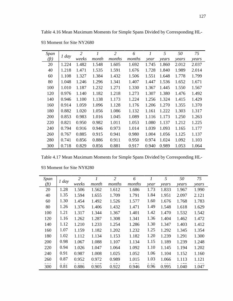
127
Table 4.16 Mean Maximum Moments for Simple Spans Divided by Corresponding HL-
93 Moment for Site NY2680
Span
(ft) 1 day
2
weeks
1
month
2
months
6
months
1
year
5
years
50
years
75
years
20 1.224 1.482 1.548 1.605 1.692 1.745 1.860 2.012 2.037
40 1.218 1.471 1.535 1.591 1.676 1.728 1.840 1.989 2.014
60 1.108 1.327 1.384 1.432 1.506 1.551 1.648 1.778 1.799
80 1.048 1.246 1.296 1.341 1.407 1.447 1.536 1.652 1.671
100 1.010 1.187 1.232 1.271 1.330 1.367 1.445 1.550 1.567
120 0.976 1.140 1.182 1.218 1.273 1.307 1.380 1.476 1.492
140 0.946 1.100 1.138 1.173 1.224 1.256 1.324 1.415 1.429
160 0.914 1.059 1.096 1.128 1.176 1.206 1.270 1.355 1.370
180 0.882 1.020 1.056 1.086 1.132 1.161 1.222 1.303 1.317
200 0.853 0.983 1.016 1.045 1.089 1.116 1.173 1.250 1.263
220 0.821 0.950 0.982 1.011 1.053 1.080 1.137 1.212 1.225
240 0.794 0.916 0.946 0.973 1.014 1.039 1.093 1.165 1.177
260 0.767 0.885 0.915 0.941 0.980 1.004 1.056 1.125 1.137
280 0.741 0.856 0.886 0.911 0.950 0.974 1.024 1.092 1.103
300 0.718 0.829 0.856 0.881 0.917 0.940 0.989 1.053 1.064
Table 4.17 Mean Maximum Moments for Simple Spans Divided by Corresponding HL-
93 Moment for Site NY8280
Span
(ft) 1 day
2
weeks
1
month
2
months
6
months
1
year
5
years
50
years
75
years
20 1.28
9 1.506 1.562 1.612 1.686 1.73
3 1.833 1.967 1.990
40 1.35
7 1.594 1.655 1.709 1.791 1.84
1 1.951 2.097 2.121
60 1.30
6 1.454 1.492 1.526 1.577 1.60
8 1.676 1.768 1.783
80 1.26
3 1.376 1.406 1.432 1.471 1.49
5 1.548 1.618 1.629
100 1.21
7 1.317 1.344 1.367 1.401 1.42
3 1.470 1.532 1.542
120 1.16
8 1.262 1.287 1.308 1.341 1.36
1 1.404 1.462 1.472
140 1.12
0 1.210 1.233 1.254 1.286 1.30
5 1.347 1.403 1.412
160 1.07
2 1.159 1.182 1.202 1.232 1.25
1 1.292 1.345 1.354
180 1.02
8 1.112 1.134 1.153 1.182 1.20
0 1.239 1.291 1.300
200 0.98
7 1.067 1.088 1.107 1.134 1.15
1 1.189 1.239 1.248
220 0.94
7 1.026 1.047 1.064 1.092 1.10
9 1.145 1.194 1.202
240 0.91
0 0.987 1.008 1.025 1.052 1.06
8 1.104 1.152 1.160
260 0.87
6 0.952 0.972 0.989 1.015 1.03
1 1.066 1.113 1.121
280 0.84
4
0.918 0.937 0.954 0.979 0.99
5
1.030 1.075 1.083 300 0.81
5 0.886 0.905 0.922 0.946 0.96
2 0.995 1.040 1.047

128
Table 4.18 Mean Maximum Moments for Simple Spans Divided by Corresponding HL-
93 Moment for Site NY8382
Span
(ft) 1 day
2
weeks
1
month
2
months
6
months
1
year
5
years
50
years
75
years
20 1.026 1.377 1.470 1.551 1.676 1.753 1.921 2.146 2.176
40 0.890 1.366 1.491 1.601 1.769 1.873 2.100 2.404 2.408
60 0.792 1.238 1.356 1.460 1.617 1.715 1.928 2.214 2.198
80 1.024 1.227 1.282 1.329 1.401 1.446 1.543 1.674 1.686
100 1.101 1.235 1.271 1.302 1.349 1.378 1.443 1.529 1.543
120 1.099 1.254 1.294 1.330 1.385 1.419 1.493 1.592 1.577
140 1.064 1.249 1.298 1.340 1.405 1.446 1.534 1.652 1.594
160 1.065 1.223 1.264 1.300 1.355 1.390 1.465 1.565 1.564
180 1.034 1.196 1.238 1.275 1.332 1.367 1.444 1.547 1.540
200 1.006 1.161 1.202 1.238 1.292 1.327 1.400 1.500 1.497
220 0.973 1.128 1.169 1.205 1.260 1.294 1.369 1.468 1.461
240 0.945 1.095 1.135 1.169 1.221 1.254 1.326 1.421 1.413
260 0.915 1.062 1.101 1.135 1.186 1.219 1.288 1.382 1.374
280 0.890 1.028 1.064 1.096 1.145 1.175 1.241 1.329 1.325
300 0.861 0.999 1.035 1.067 1.116 1.146 1.212 1.300 1.292
Table 4.19 Mean Maximum Moments for Simple Spans Divided by Corresponding HL-
93 Moment for Site NY9121
Span
(ft) 1 day
2
weeks
1
month
2
months
6
months
1
year
5
years
50
years
75
years
20 1.076 1.393 1.476 1.549 1.661 1.730 1.880 2.082 2.116
40 1.045 1.366 1.451 1.524 1.637 1.707 1.860 2.064 2.098
60 0.971 1.248 1.322 1.386 1.483 1.544 1.676 1.852 1.882
80 0.963 1.184 1.241 1.292 1.370 1.418 1.522 1.662 1.686
100 0.982 1.144 1.187 1.224 1.281 1.317 1.394 1.497 1.515
120 0.974 1.117 1.155 1.187 1.238 1.269 1.337 1.428 1.443
140 0.951 1.091 1.127 1.160 1.209 1.240 1.306 1.395 1.410
160 0.924 1.064 1.100 1.132 1.181 1.211 1.277 1.366 1.381
180 0.896 1.034 1.070 1.102 1.150 1.180 1.245 1.332 1.347
200 0.869 1.005 1.041 1.072 1.120 1.150 1.214 1.300 1.315
220 0.843 0.975 1.010 1.040 1.087 1.116 1.179 1.262 1.277
240 0.818 0.946 0.980 1.010 1.056 1.083 1.144 1.227 1.240
260 0.795 0.918 0.950 0.979 1.023 1.050 1.108 1.187 1.200
280 0.770 0.891 0.922 0.950 0.993 1.019 1.077 1.154 1.167
300 0.751 0.864 0.893 0.920 0.959 0.984 1.038 1.110 1.121
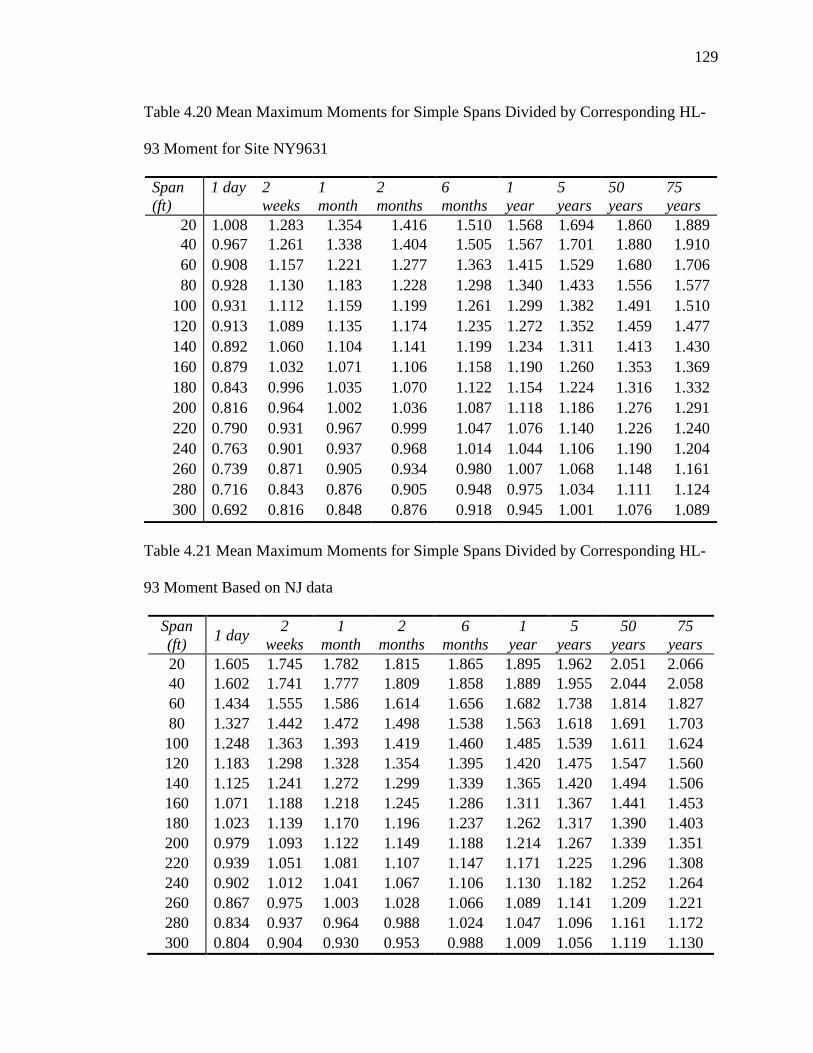
129
Table 4.20 Mean Maximum Moments for Simple Spans Divided by Corresponding HL-
93 Moment for Site NY9631
Span
(ft)
1 day 2
weeks
1
month
2
months
6
months
1
year
5
years
50
years
75
years
20 1.008 1.283 1.354 1.416 1.510 1.568 1.694 1.860 1.889
40 0.967 1.261 1.338 1.404 1.505 1.567 1.701 1.880 1.910
60 0.908 1.157 1.221 1.277 1.363 1.415 1.529 1.680 1.706
80 0.928 1.130 1.183 1.228 1.298 1.340 1.433 1.556 1.577
100 0.931 1.112 1.159 1.199 1.261 1.299 1.382 1.491 1.510
120 0.913 1.089 1.135 1.174 1.235 1.272 1.352 1.459 1.477
140 0.892 1.060 1.104 1.141 1.199 1.234 1.311 1.413 1.430
160 0.879 1.032 1.071 1.106 1.158 1.190 1.260 1.353 1.369
180 0.843 0.996 1.035 1.070 1.122 1.154 1.224 1.316 1.332
200 0.816 0.964 1.002 1.036 1.087 1.118 1.186 1.276 1.291
220 0.790 0.931 0.967 0.999 1.047 1.076 1.140 1.226 1.240
240 0.763 0.901 0.937 0.968 1.014 1.044 1.106 1.190 1.204
260 0.739 0.871 0.905 0.934 0.980 1.007 1.068 1.148 1.161
280 0.716 0.843 0.876 0.905 0.948 0.975 1.034 1.111 1.124
300 0.692 0.816 0.848 0.876 0.918 0.945 1.001 1.076 1.089
Table 4.21 Mean Maximum Moments for Simple Spans Divided by Corresponding HL-
93 Moment Based on NJ data
Span
(ft) 1 day
2
weeks
1
month
2
months
6
months
1
year
5
years
50
years
75
years
20 1.605 1.745 1.782 1.815 1.865 1.895 1.962 2.051 2.066
40 1.602 1.741 1.777 1.809 1.858 1.889 1.955 2.044 2.058
60 1.434 1.555 1.586 1.614 1.656 1.682 1.738 1.814 1.827
80 1.327 1.442 1.472 1.498 1.538 1.563 1.618 1.691 1.703
100 1.248 1.363 1.393 1.419 1.460 1.485 1.539 1.611 1.624
120 1.183 1.298 1.328 1.354 1.395 1.420 1.475 1.547 1.560
140 1.125 1.241 1.272 1.299 1.339 1.365 1.420 1.494 1.506
160 1.071 1.188 1.218 1.245 1.286 1.311 1.367 1.441 1.453
180 1.023 1.139 1.170 1.196 1.237 1.262 1.317 1.390 1.403
200 0.979 1.093 1.122 1.149 1.188 1.214 1.267 1.339 1.351
220 0.939 1.051 1.081 1.107 1.147 1.171 1.225 1.296 1.308
240 0.902 1.012 1.041 1.067 1.106 1.130 1.182 1.252 1.264
260 0.867 0.975 1.003 1.028 1.066 1.089 1.141 1.209 1.221
280 0.834 0.937 0.964 0.988 1.024 1.047 1.096 1.161 1.172
300 0.804 0.904 0.930 0.953 0.988 1.009 1.056 1.119 1.130

130
4.2.3.2 Comparison between Different WIM Sites
Figure 4.18 through Figure 4.35 show the comparison of load effects between
various WIM sites at various return periods. It is observed that except site 8332, there is
no significant difference between the long term load effects calculated from NJ data and
NY data. The average difference ranges from 3.1% to 7.9%, 1.1% to 4.4%, and 1.3% to
4.5%, respectively, for upper 20% extension, re-plot extrapolation, and normal
approximation method. It is also observed that the difference of the long term
predication between NY site 8382 and other WIM sites is larger with an average
difference of 8.7%, 11.3%, and 10.9% respectively for upper 20% extension; re-plot
extrapolation, and normal approximation method. This phenomenon can be caused by
large number of heavy vehicle that collected from NY 8382 site. There are 649 trucks
above 150 kips while site 9021 only has 219 trucks above 150 kips.
Figure 4.18 Comparison of Moment Ratio for Various WIM Sites (1 day period)
0.6
0.8
1
1.2
1.4
1.6
1.8
0 50 100 150 200 250 300 350
1 Day NY 0199-NB
NY 0199-SB
NY 0580
NY 2680
NY 8280
NY 8382
NY 9121
NY 9631
NJ data
Mea
n M
om
ent
/ HL
93
Span (ft)
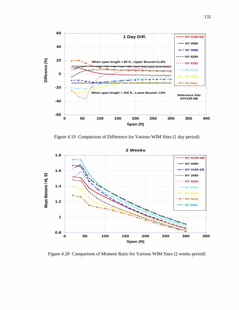
131
Figure 4.19 Comparison of Difference for Various WIM Sites (1 day period)
Figure 4.20 Comparison of Moment Ratio for Various WIM Sites (2 weeks period)
-60
-40
-20
0
20
40
60
0 50 100 150 200 250 300 350 400
1 Day Diff. NY 0199-SB
NY 0580
NY 2680
NY 8280
NY 8382
NY 9121
NY 9631
NJ data
Dif
fere
nc
e (
%)
Span (ft)
When span length > 80 ft., Upper Bound=11.8%
When span length > 160 ft., Lower Bound=-13%Reference Site:
NY0199-NB
0.8
1
1.2
1.4
1.6
1.8
0 50 100 150 200 250 300 350
2 Weeks
NY 0199-NB
NY 0580
NY 0199-SB
NY 2680
NY 8280
NY 8382
NY 9121
NY 9631
NJ data
Mea
n M
omen
t / H
L 9
3
Span (ft)

132
Figure 4.21 Comparison of Difference for Various WIM Sites (2 weeks period)
Figure 4.22 Comparison of Moment Ratio for Various WIM Sites (1 month period)
-60
-40
-20
0
20
40
60
0 50 100 150 200 250 300 350 400
2 Weeks Diff. NY 0199-SB
NY 0580
NY 2680
NY 8280
NY 8382
NY 9121
NY 9631
NJ data
Dif
fere
nc
e (
%)
Span (ft)
When span length > 100 ft., Upper Bound=7.9%
When span length > 140 ft., Lower Bound=-7.1%
Reference Site:
NY0199-NB
0.8
1
1.2
1.4
1.6
1.8
0 50 100 150 200 250 300 350
1 Month
NY 0199-NB
NY 0580
NY 0199-SB
NY 2680
NY 8280
NY 8382
NY 9121
NY 9631
NJ data
Mea
n M
omen
t / H
L 9
3
Span (ft)
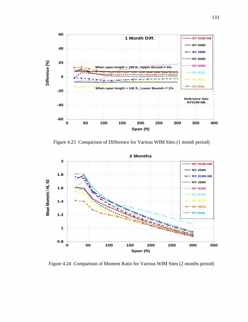
133
Figure 4.23 Comparison of Difference for Various WIM Sites (1 month period)
Figure 4.24 Comparison of Moment Ratio for Various WIM Sites (2 months period)
-60
-40
-20
0
20
40
60
0 50 100 150 200 250 300 350 400
1 Month Diff. NY 0199-SB
NY 0580
NY 2680
NY 8280
NY 8382
NY 9121
NY 9631
NJ data
Dif
fere
nc
e (
%)
Span (ft)
When span length > 100 ft., Upper Bound=7.9%
When span length > 140 ft., Lower Bound=-7.1%
Reference Site:
NY0199-NB
0.8
1
1.2
1.4
1.6
1.8
2
0 50 100 150 200 250 300 350
2 Months
NY 0199-NB
NY 0580
NY 0199-SB
NY 2680
NY 8280
NY 8382
NY 9121
NY 9631
NJ data
Mea
n M
omen
t / H
L 9
3
Span (ft)
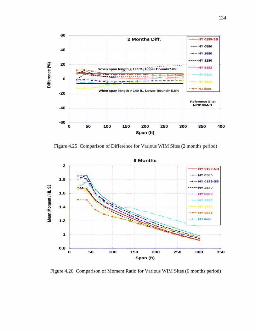
134
Figure 4.25 Comparison of Difference for Various WIM Sites (2 months period)
Figure 4.26 Comparison of Moment Ratio for Various WIM Sites (6 months period)
-60
-40
-20
0
20
40
60
0 50 100 150 200 250 300 350 400
2 Months Diff. NY 0199-SB
NY 0580
NY 2680
NY 8280
NY 8382
NY 9121
NY 9631
NJ data
Dif
fere
nc
e (
%)
Span (ft)
When span length > 100 ft., Upper Bound=7.6%
When span length > 140 ft., Lower Bound=-5.8%
Reference Site:
NY0199-NB
0.8
1
1.2
1.4
1.6
1.8
2
0 50 100 150 200 250 300 350
6 Months
NY 0199-NB
NY 0580
NY 0199-SB
NY 2680
NY 8280
NY 8382
NY 9121
NY 9631
NJ dataMea
n M
omen
t / H
L 9
3
Span (ft)

135
Figure 4.27 Comparison of Difference for Various WIM Sites (6 months period)
Figure 4.28 Comparison of Moment Ratio for Various WIM Sites (1 year period)
-60
-40
-20
0
20
40
60
0 50 100 150 200 250 300 350 400
6 Months Diff. NY 0199-SB
NY 0580
NY 2680
NY 8280
NY 8382
NY 9121
NY 9631
NJ data
Dif
fere
nc
e (
%)
Span (ft)
When span length > 60 ft., Upper Bound=8.5%
When span length > 140 ft., Lower Bound=-4.1%
Reference Site:
NY0199-NB
0.8
1
1.2
1.4
1.6
1.8
2
2.2
2.4
0 50 100 150 200 250 300 350
1 Year
NY 0199-NB
NY 0580
NY 0199-SB
NY 2680
NY 8280
NY 8382
NY 9121
NY 9631
NJ data
Mea
n M
omen
t / H
L 9
3
Span (ft)

136
Figure 4.29 Comparison of Difference for Various WIM Sites (1 year period)
Figure 4.30 Comparison of Moment Ratio for Various WIM Sites (5 years period)
-60
-40
-20
0
20
40
60
0 50 100 150 200 250 300 350 400
1 Year Diff. NY 0199-SB
NY 0580
NY 2680
NY 8280
NY 8382
NY 9121
NY 9631
NJ data
Dif
fere
nc
e (
%)
Span (ft)
When span length > 60 ft., Upper Bound=8.3%
When span length > 140 ft., Lower Bound=-3.1%
Reference Site:
NY0199-NB
0.8
1
1.2
1.4
1.6
1.8
2
2.2
2.4
0 50 100 150 200 250 300 350
5 Year
NY 0199-NB
NY 0580
NY 0199-SB
NY 2680
NY 8280
NY 8382
NY 9121
NY 9631
NJ data
Mea
n M
omen
t / H
L 9
3
Span (ft)
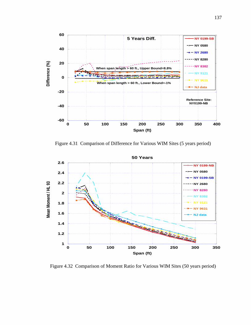
137
Figure 4.31 Comparison of Difference for Various WIM Sites (5 years period)
Figure 4.32 Comparison of Moment Ratio for Various WIM Sites (50 years period)
-60
-40
-20
0
20
40
60
0 50 100 150 200 250 300 350 400
5 Years Diff. NY 0199-SB
NY 0580
NY 2680
NY 8280
NY 8382
NY 9121
NY 9631
NJ data
Dif
fere
nc
e (
%)
Span (ft)
When span length > 60 ft., Upper Bound=8.8%
When span length > 60 ft., Lower Bound=-1%
Reference Site:
NY0199-NB
1
1.2
1.4
1.6
1.8
2
2.2
2.4
2.6
0 50 100 150 200 250 300 350
50 Years
NY 0199-NB
NY 0580
NY 0199-SB
NY 2680
NY 8280
NY 8382
NY 9121
NY 9631
NJ data
Mea
n M
omen
t / H
L 9
3
Span (ft)
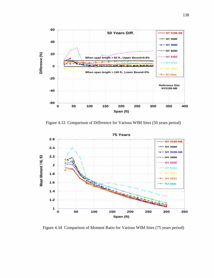
138
Figure 4.33 Comparison of Difference for Various WIM Sites (50 years period)
Figure 4.34 Comparison of Moment Ratio for Various WIM Sites (75 years period)
-60
-40
-20
0
20
40
60
0 50 100 150 200 250 300 350 400
50 Years Diff. NY 0199-SB
NY 0580
NY 2680
NY 8280
NY 8382
NY 9121
NY 9631
NJ data
Dif
fere
nc
e (
%)
Span (ft)
When span length > 60 ft., Upper Bound=9.6%
When span length > 140 ft., Lower Bound=0%
Reference Site:
NY0199-NB
1
1.2
1.4
1.6
1.8
2
2.2
2.4
2.6
0 50 100 150 200 250 300 350
75 Years
NY 0199-NB
NY 0580
NY 0199-SB
NY 2680
NY 8280
NY 8382
NY 9121
NY 9631
NJ data
Mea
n M
omen
t / H
L 9
3
Span (ft)

139
Figure 4.35 Comparison of Difference for Various WIM Sites (75 years period)
4.2.3.3 Effects of Extrapolation Methods
In section 4.2.2, various probabilistic extrapolation methods were discussed. In
order to compare the outcome of each extrapolation methods, the bias factors that were
calculated using different extrapolation methods including manual linear extension, up
20% extrapolation, re-plot of 20% extrapolation and normal approximation prediction
were present for four typical New York WIM sites. Considerable difference is observed
between manual linear extension and other methods.
-60
-40
-20
0
20
40
60
0 50 100 150 200 250 300 350 400
75 Years Diff. NY 0199-SB
NY 0580
NY 2680
NY 8280
NY 8382
NY 9121
NY 9631
NJ data
Dif
fere
nc
e (
%)
Span (ft)
When span length > 60 ft., Upper Bound=9.7%
When span length > 140 ft., Lower Bound=0.1%
Reference Site:
NY0199-NB
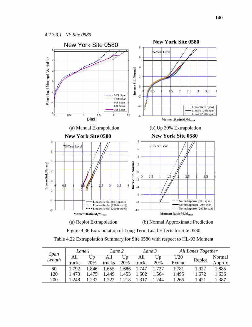
140
4.2.3.3.1 NY Site 0580
(a) Manual Extrapolation (b) Up 20% Extrapolation
(a) Replot Extrapolation (b) Normal Approximate Prediction
Figure 4.36 Extrapolation of Long Term Load Effects for Site 0580
Table 4.22 Extrapolation Summary for Site 0580 with respect to HL-93 Moment
Span
Length
Lane 1 Lane 2 Lane 3 All Lanes Together
All
trucks
Up
20%
All
trucks
Up
20%
All
trucks
Up
20%
U20
Extend Replot
Normal
Approx
60 1.792 1.846 1.655 1.686 1.747 1.727 1.781 1.927 1.885 120 1.473 1.475 1.449 1.453 1.602 1.564 1.495 1.672 1.636
200 1.248 1.232 1.222 1.218 1.317 1.244 1.265 1.421 1.387
0 0.5 1 1.5 2 2.5-6
-4
-2
0
2
4
6
Bias
Sta
ndard
Norm
al V
ariable
New York Site 0580
200ft Span
120ft Span
90ft Span
60ft Span
30ft Span
-6
-4
-2
0
2
4
6
8
0 0.5 1 1.5 2 2.5 3 3.5 4
Inv
erse
Std
. No
rma
l
Moment Ratio Mi/MHS20
Linear (60ft Span)
Linear (120ft Span)
Linear (200ft Span)
75-Year Level
New York Site 0580
-6
-4
-2
0
2
4
6
8
0 0.5 1 1.5 2 2.5 3 3.5 4
Inv
erse
Std
. No
rma
l
Moment Ratio Mi/MHS20
Linear (Replot (60 ft span))
Linear (Replot (120 ft span))
Linear (Replot (200 ft span))
75-Year Level
New York Site 0580
-10
-8
-6
-4
-2
0
2
4
6
8
0 0.5 1 1.5 2 2.5 3 3.5 4
Inv
erse
Std
. No
rma
l
Moment Ratio Mi/MHS20
NormalApprox (60 ft span)
NormalApprox(120 ft span)
NormalApprox (200 ft span)
75-Year Level
New York Site 0580
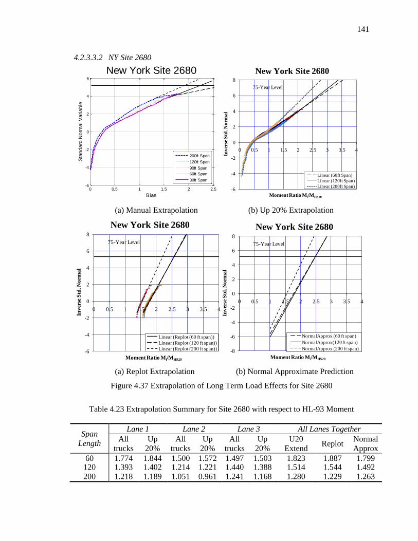
141
4.2.3.3.2 NY Site 2680
(a) Manual Extrapolation (b) Up 20% Extrapolation
(a) Replot Extrapolation (b) Normal Approximate Prediction
Figure 4.37 Extrapolation of Long Term Load Effects for Site 2680
Table 4.23 Extrapolation Summary for Site 2680 with respect to HL-93 Moment
Span
Length
Lane 1 Lane 2 Lane 3 All Lanes Together
All
trucks
Up
20%
All
trucks
Up
20%
All
trucks
Up
20%
U20
Extend Replot
Normal
Approx
60 1.774 1.844 1.500 1.572 1.497 1.503 1.823 1.887 1.799 120 1.393 1.402 1.214 1.221 1.440 1.388 1.514 1.544 1.492
200 1.218 1.189 1.051 0.961 1.241 1.168 1.280 1.229 1.263
0 0.5 1 1.5 2 2.5-6
-4
-2
0
2
4
6
Bias
Sta
nd
ard
No
rma
l V
ari
ab
le
New York Site 2680
200ft Span
120ft Span
90ft Span
60ft Span
30ft Span
-6
-4
-2
0
2
4
6
8
0 0.5 1 1.5 2 2.5 3 3.5 4
Inv
erse
Std
. No
rma
l
Moment Ratio Mi/MHS20
Linear (60ft Span)
Linear (120ft Span)
Linear (200ft Span)
75-Year Level
New York Site 2680
-6
-4
-2
0
2
4
6
8
0 0.5 1 1.5 2 2.5 3 3.5 4
Inv
erse
Std
. No
rma
l
Moment Ratio Mi/MHS20
Linear (Replot (60 ft span))
Linear (Replot (120 ft span))
Linear (Replot (200 ft span))
75-Year Level
New York Site 2680
-8
-6
-4
-2
0
2
4
6
8
0 0.5 1 1.5 2 2.5 3 3.5 4
Inv
erse
Std
. No
rma
l
Moment Ratio Mi/MHS20
NormalApprox (60 ft span)
NormalApprox(120 ft span)
NormalApprox (200 ft span)
75-Year Level
New York Site 2680
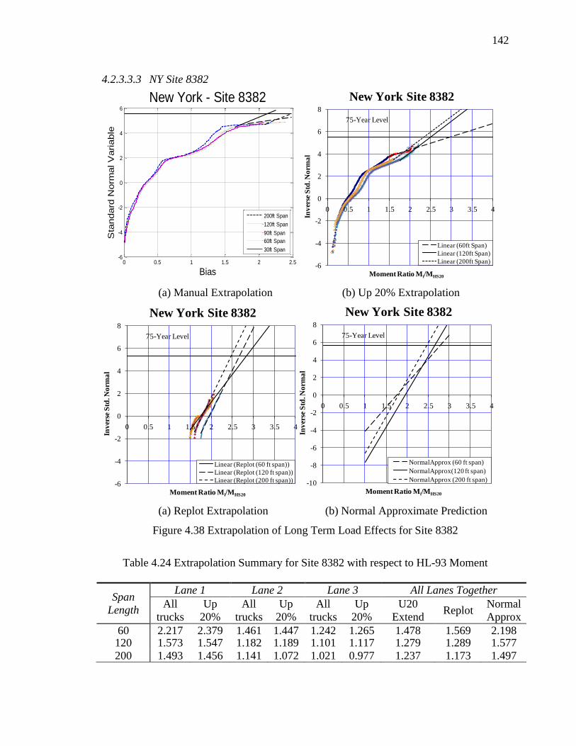
142
4.2.3.3.3 NY Site 8382
(a) Manual Extrapolation (b) Up 20% Extrapolation
(a) Replot Extrapolation (b) Normal Approximate Prediction
Figure 4.38 Extrapolation of Long Term Load Effects for Site 8382
Table 4.24 Extrapolation Summary for Site 8382 with respect to HL-93 Moment
Span
Length
Lane 1 Lane 2 Lane 3 All Lanes Together
All
trucks
Up
20%
All
trucks
Up
20%
All
trucks
Up
20%
U20
Extend Replot
Normal
Approx
60 2.217 2.379 1.461 1.447 1.242 1.265 1.478 1.569 2.198 120 1.573 1.547 1.182 1.189 1.101 1.117 1.279 1.289 1.577
200 1.493 1.456 1.141 1.072 1.021 0.977 1.237 1.173 1.497
0 0.5 1 1.5 2 2.5-6
-4
-2
0
2
4
6
Bias
Sta
ndard
Norm
al V
ariable
New York - Site 8382
200ft Span
120ft Span
90ft Span
60ft Span
30ft Span
-6
-4
-2
0
2
4
6
8
0 0.5 1 1.5 2 2.5 3 3.5 4
Inv
erse
Std
. No
rma
l
Moment Ratio Mi/MHS20
Linear (60ft Span)
Linear (120ft Span)
Linear (200ft Span)
75-Year Level
New York Site 8382
-6
-4
-2
0
2
4
6
8
0 0.5 1 1.5 2 2.5 3 3.5 4
Inv
erse
Std
. No
rma
l
Moment Ratio Mi/MHS20
Linear (Replot (60 ft span))
Linear (Replot (120 ft span))
Linear (Replot (200 ft span))
75-Year Level
New York Site 8382
-10
-8
-6
-4
-2
0
2
4
6
8
0 0.5 1 1.5 2 2.5 3 3.5 4
Inv
erse
Std
. No
rma
l
Moment Ratio Mi/MHS20
NormalApprox (60 ft span)
NormalApprox(120 ft span)
NormalApprox (200 ft span)
75-Year Level
New York Site 8382
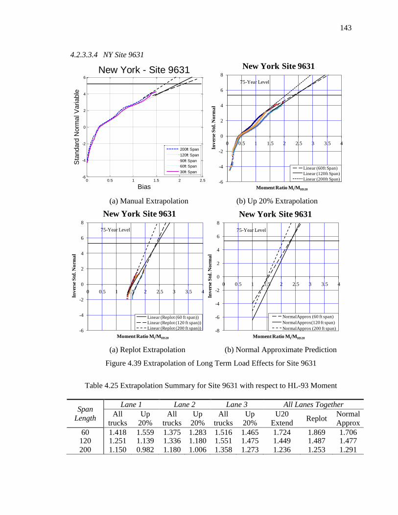
143
4.2.3.3.4 NY Site 9631
(a) Manual Extrapolation (b) Up 20% Extrapolation
(a) Replot Extrapolation (b) Normal Approximate Prediction
Figure 4.39 Extrapolation of Long Term Load Effects for Site 9631
Table 4.25 Extrapolation Summary for Site 9631 with respect to HL-93 Moment
Span
Length
Lane 1 Lane 2 Lane 3 All Lanes Together
All
trucks
Up
20%
All
trucks
Up
20%
All
trucks
Up
20%
U20
Extend Replot
Normal
Approx
60 1.418 1.559 1.375 1.283 1.516 1.465 1.724 1.869 1.706 120 1.251 1.139 1.336 1.180 1.551 1.475 1.449 1.487 1.477
200 1.150 0.982 1.180 1.006 1.358 1.273 1.236 1.253 1.291
0 0.5 1 1.5 2 2.5-6
-4
-2
0
2
4
6
Bias
Sta
ndard
Norm
al V
ariable
New York - Site 9631
200ft Span
120ft Span
90ft Span
60ft Span
30ft Span
-6
-4
-2
0
2
4
6
8
0 0.5 1 1.5 2 2.5 3 3.5 4
Inv
erse
Std
. No
rma
l
Moment Ratio Mi/MHS20
Linear (60ft Span)
Linear (120ft Span)
Linear (200ft Span)
75-Year Level
New York Site 9631
-6
-4
-2
0
2
4
6
8
0 0.5 1 1.5 2 2.5 3 3.5 4
Inv
erse
Std
. No
rma
l
Moment Ratio Mi/MHS20
Linear (Replot (60 ft span))
Linear (Replot (120 ft span))
Linear (Replot (200 ft span))
75-Year Level
New York Site 9631
-8
-6
-4
-2
0
2
4
6
8
0 0.5 1 1.5 2 2.5 3 3.5 4
Inv
erse
Std
. No
rma
l
Moment Ratio Mi/MHS20
NormalApprox (60 ft span)
NormalApprox(120 ft span)
NormalApprox (200 ft span)
75-Year Level
New York Site 9631

144
4.3 Proposed Live Load Models
Although WIM data from many states have been investigated and their site
specific live load effects were studied, the live load models that proposed to be used in
this study were developed based on NCHRP and FWHA Weigh-in-Motion (WIM)
database which contains 32 different WIM sites. For each site, approximately 1 year (12
months) of data was collected and the data was processed using a filtering program to
remove the errors and permit vehicles.
A live load model for reliability analysis is defined with two parameters using HL-93
vehicle model as a reference. These two parameters are the bias factor and the coefficient of
variation. The bias factor is a mean to nominal ratio between the mean maximum load effect (i.e.
moment and shear) from WIM data and load effect from HL-93 Load. Moreover, due to the
fact that the traffic volumes are different for different states and locations, the load
models were developed for various traffic volume levels (i.e. Average Daily Truck
Traffic (ADTT) of 1000, 2500, 5000, 10000). The following sections presents the live
load models used in this study for various ADTT levels and various serviceability limit
states.
4.3.1 Proposed Live Load Model for Service I Limit State
Since the reinforced concrete deck was designed for axle load, the axle load data
including steering axle collected from 32 different WIM sites was processed using a
quality control filtering routine. The cumulative distribution functions (CDF) of
processed axle load data was plotted on a normal probability paper. The vertical
coordinate of maximum axle weight, maxz , is calculated using the equation below:
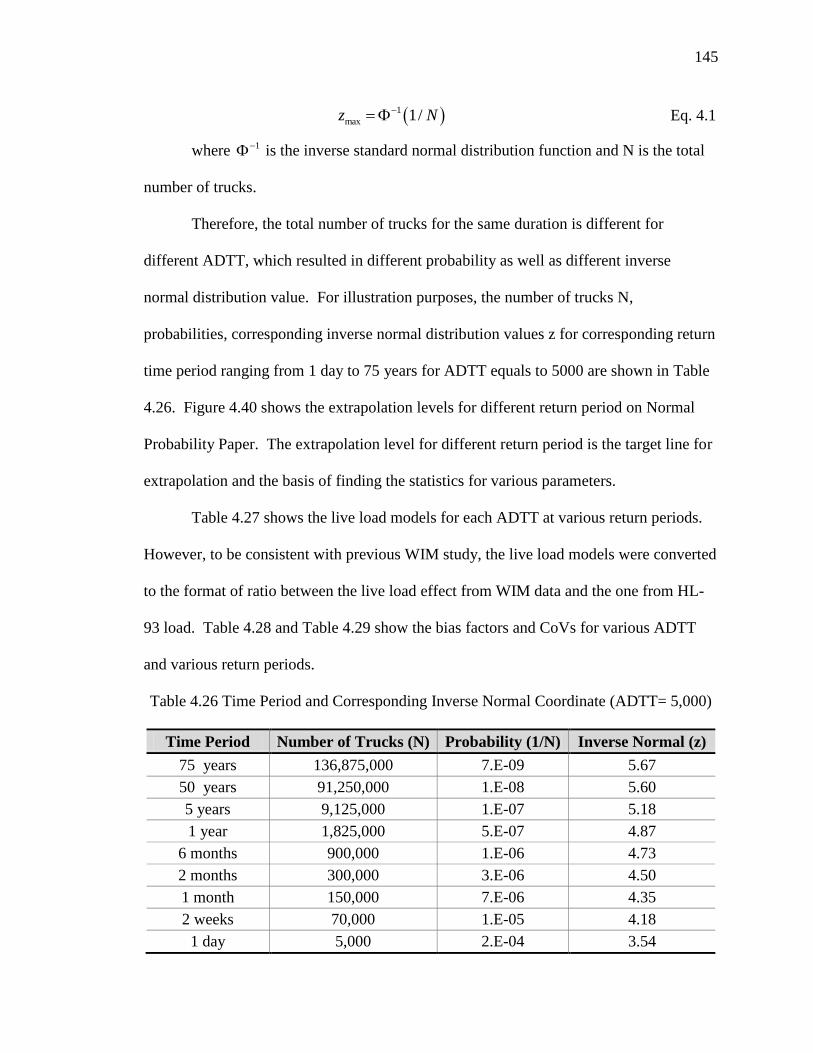
145
1
max 1/z N Eq. 4.1
where 1 is the inverse standard normal distribution function and N is the total
number of trucks.
Therefore, the total number of trucks for the same duration is different for
different ADTT, which resulted in different probability as well as different inverse
normal distribution value. For illustration purposes, the number of trucks N,
probabilities, corresponding inverse normal distribution values z for corresponding return
time period ranging from 1 day to 75 years for ADTT equals to 5000 are shown in Table
4.26. Figure 4.40 shows the extrapolation levels for different return period on Normal
Probability Paper. The extrapolation level for different return period is the target line for
extrapolation and the basis of finding the statistics for various parameters.
Table 4.27 shows the live load models for each ADTT at various return periods.
However, to be consistent with previous WIM study, the live load models were converted
to the format of ratio between the live load effect from WIM data and the one from HL-
93 load. Table 4.28 and Table 4.29 show the bias factors and CoVs for various ADTT
and various return periods.
Table 4.26 Time Period and Corresponding Inverse Normal Coordinate (ADTT= 5,000)
Time Period Number of Trucks (N) Probability (1/N) Inverse Normal (z)
75 years 136,875,000 7.E-09 5.67
50 years 91,250,000 1.E-08 5.60
5 years 9,125,000 1.E-07 5.18
1 year 1,825,000 5.E-07 4.87
6 months 900,000 1.E-06 4.73
2 months 300,000 3.E-06 4.50
1 month 150,000 7.E-06 4.35
2 weeks 70,000 1.E-05 4.18
1 day 5,000 2.E-04 3.54
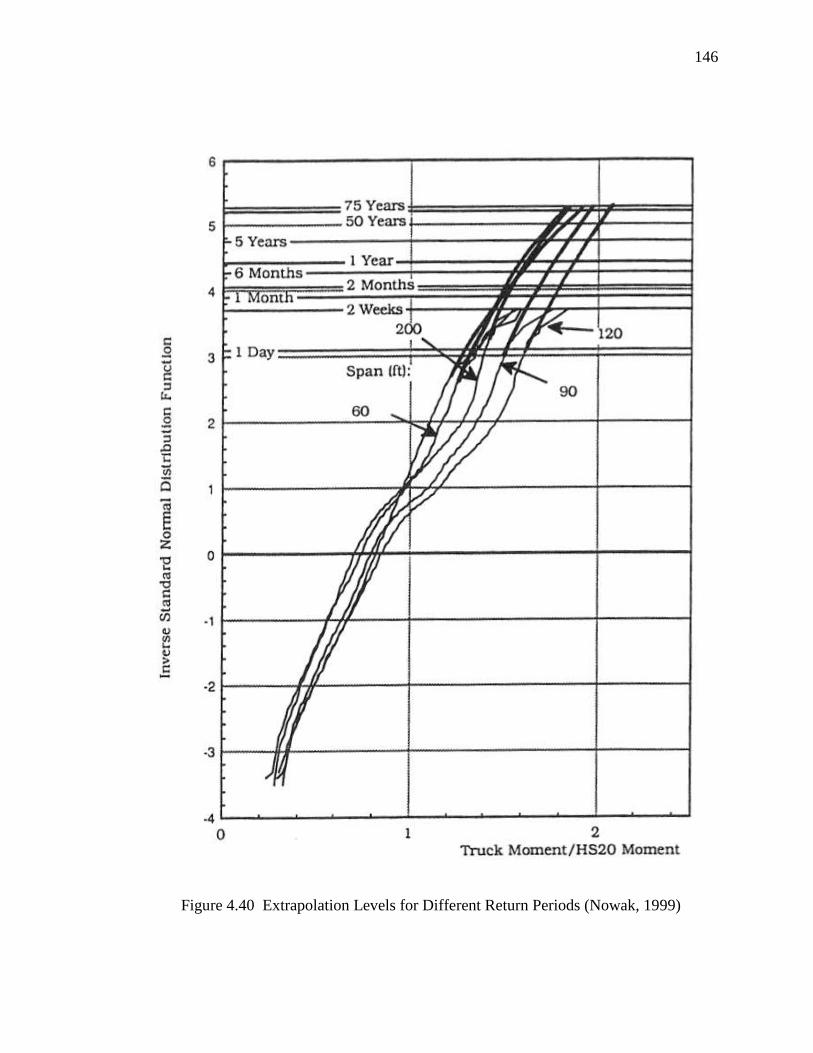
146
Figure 4.40 Extrapolation Levels for Different Return Periods (Nowak, 1999)
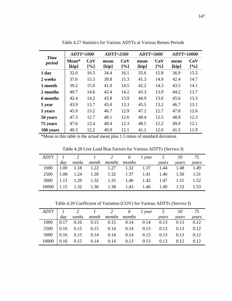
147
Table 4.27 Statistics for Various ADTTs at Various Return Periods
Time
period
ADTT=1000 ADTT=2500 ADTT=5000 ADTT=10000
Mean*
[kip]
CoV
[%]
mean
[kip]
CoV
[%]
mean
[kip]
CoV
[%]
mean
[kip]
CoV
[%]
1 day 32.0 16.5 34.4 16.1 35.6 15.8 36.9 15.5
2 weeks 37.6 15.5 39.8 15.3 41.3 14.9 42.4 14.7
1 month 39.2 15.0 41.0 14.5 42.2 14.3 43.5 14.1
2 months 40.7 14.6 42.4 14.2 43.3 13.9 44.2 13.7
6 months 42.4 14.2 43.8 13.9 44.9 13.6 45.6 13.3
1 year 43.9 13.7 45.0 13.3 45.5 13.2 46.7 13.1
5 years 45.9 13.2 46.7 12.9 47.2 12.7 47.8 12.6
50 years 47.3 12.7 48.1 12.6 48.4 12.5 48.8 12.3
75 years 47.6 12.4 48.4 12.3 48.5 12.2 49.0 12.1
100 years 40.3 12.2 40.9 12.1 41.1 12.0 41.5 11.9
*Mean in this table is the actual mean plus 1.5 times of standard deviation.
Table 4.28 Live Load Bias Factors for Various ADTTs (Service I)
ADTT 1
day
2
weeks
1
month
2
months
6
months
1 year 5
years
50
years
75
years
1000 1.00 1.18 1.22 1.27 1.32 1.37 1.44 1.48 1.49
2500 1.08 1.24 1.28 1.32 1.37 1.41 1.46 1.50 1.51
5000 1.11 1.29 1.32 1.35 1.40 1.42 1.47 1.51 1.52
10000 1.15 1.32 1.36 1.38 1.43 1.46 1.49 1.53 1.53
Table 4.29 Coefficient of Variation (COV) for Various ADTTs (Service I)
ADTT 1
day
2
weeks
1
month
2
months
6
months
1 year 5
years
50
years
75
years
1000 0.17 0.16 0.15 0.15 0.14 0.14 0.13 0.13 0.12
2500 0.16 0.15 0.15 0.14 0.14 0.13 0.13 0.13 0.12
5000 0.16 0.15 0.14 0.14 0.14 0.13 0.13 0.13 0.12
10000 0.16 0.15 0.14 0.14 0.13 0.13 0.13 0.12 0.12

148
4.3.2 Proposed Live Load Model for Regular Truck Load for Service III Limit State
Similar to the live load model shown in Section 4.3.1 for Service I limit state, the
same procedure was followed to develop the live load model for regular truck load for
Service III limit state except the moment due to whole truck was considered instead of
load effect due to axle load. The live load statistical information was derived from
NCHRP and FWHA Weigh-in-Motion (WIM) database. The live load bias factors and
coefficient of variation for various average daily truck traffic (ADTT) (1000, 2500, 5000,
and 10000) are summarized in Table 4.38 through Table 4.41. Based on NCHRP 368
Report, The mean and standard deviation of dynamic load factor was taken as 0.09 and
0.05, respectively.
Table 4.30 Live Load Bias Factors for Various Span Lengths (ADTT=1000)
Span
(ft)
1 day 2
weeks
1
month
2
months
6
months
1 year 5
years
50
years
75
years
30 ft 0.99 1.14 1.18 1.23 1.27 1.33 1.37 1.38 1.4
60 ft 0.89 1.13 1.19 1.26 1.31 1.34 1.37 1.42 1.42
90 ft 0.9 1.13 1.19 1.26 1.3 1.32 1.36 1.41 1.42
120 ft 0.89 1.14 1.19 1.23 1.27 1.31 1.35 1.41 1.41
200 ft 0.81 1.06 1.11 1.16 1.22 1.25 1.3 1.35 1.36
300 ft 0.71 0.97 1.01 1.07 1.15 1.18 1.24 1.28 1.29
Table 4.31 Coefficient of Variation (COV) for Various Span Lengths (ADTT=1000)
Span
(ft)
1 day 2
weeks
1
month
2
months
6
months
1 year 5
years
50
years
75
years
30 ft 0.28 0.21 0.16 0.16 0.14 0.16 0.15 0.07 0.07
60 ft 0.2 0.16 0.16 0.18 0.16 0.16 0.13 0.12 0.11
90 ft 0.17 0.18 0.17 0.17 0.12 0.1 0.08 0.08 0.07
120 ft 0.17 0.16 0.16 0.13 0.11 0.1 0.1 0.11 0.1
200 ft 0.19 0.16 0.14 0.14 0.15 0.16 0.15 0.14 0.13
300 ft 0.19 0.16 0.14 0.14 0.15 0.16 0.15 0.14 0.13
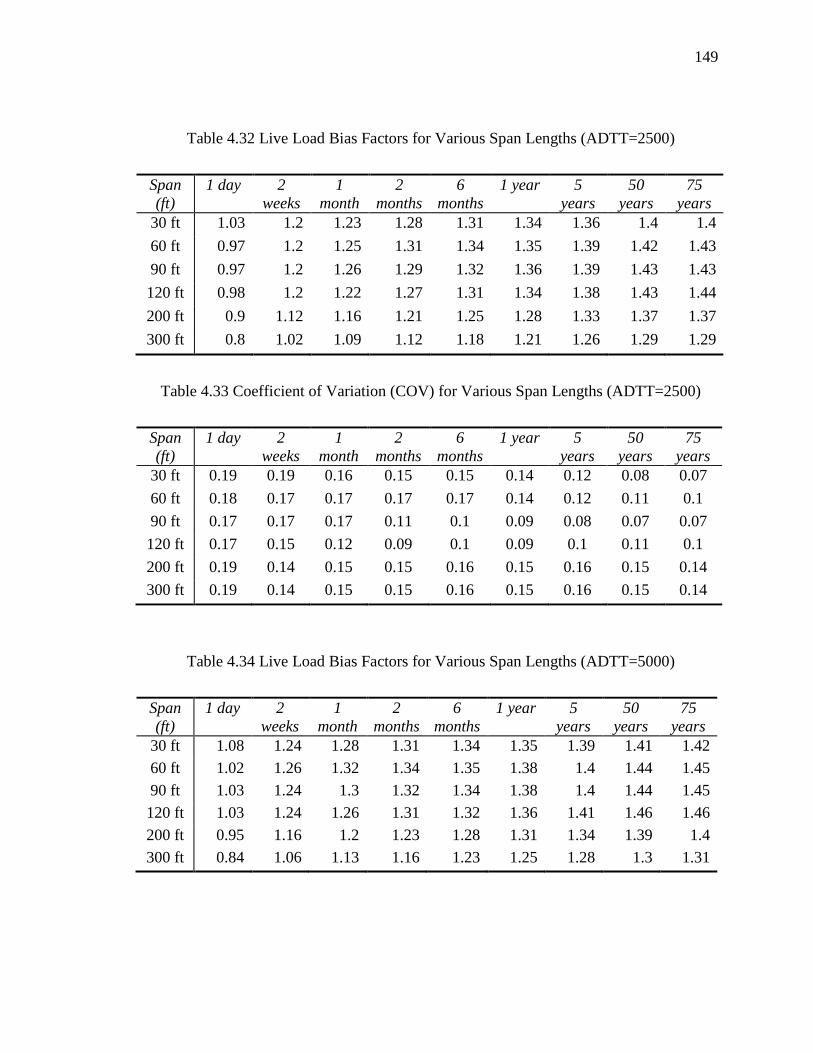
149
Table 4.32 Live Load Bias Factors for Various Span Lengths (ADTT=2500)
Span
(ft)
1 day 2
weeks
1
month
2
months
6
months
1 year 5
years
50
years
75
years
30 ft 1.03 1.2 1.23 1.28 1.31 1.34 1.36 1.4 1.4
60 ft 0.97 1.2 1.25 1.31 1.34 1.35 1.39 1.42 1.43
90 ft 0.97 1.2 1.26 1.29 1.32 1.36 1.39 1.43 1.43
120 ft 0.98 1.2 1.22 1.27 1.31 1.34 1.38 1.43 1.44
200 ft 0.9 1.12 1.16 1.21 1.25 1.28 1.33 1.37 1.37
300 ft 0.8 1.02 1.09 1.12 1.18 1.21 1.26 1.29 1.29
Table 4.33 Coefficient of Variation (COV) for Various Span Lengths (ADTT=2500)
Span
(ft)
1 day 2
weeks
1
month
2
months
6
months
1 year 5
years
50
years
75
years
30 ft 0.19 0.19 0.16 0.15 0.15 0.14 0.12 0.08 0.07
60 ft 0.18 0.17 0.17 0.17 0.17 0.14 0.12 0.11 0.1
90 ft 0.17 0.17 0.17 0.11 0.1 0.09 0.08 0.07 0.07
120 ft 0.17 0.15 0.12 0.09 0.1 0.09 0.1 0.11 0.1
200 ft 0.19 0.14 0.15 0.15 0.16 0.15 0.16 0.15 0.14
300 ft 0.19 0.14 0.15 0.15 0.16 0.15 0.16 0.15 0.14
Table 4.34 Live Load Bias Factors for Various Span Lengths (ADTT=5000)
Span
(ft)
1 day 2
weeks
1
month
2
months
6
months
1 year 5
years
50
years
75
years
30 ft 1.08 1.24 1.28 1.31 1.34 1.35 1.39 1.41 1.42
60 ft 1.02 1.26 1.32 1.34 1.35 1.38 1.4 1.44 1.45
90 ft 1.03 1.24 1.3 1.32 1.34 1.38 1.4 1.44 1.45
120 ft 1.03 1.24 1.26 1.31 1.32 1.36 1.41 1.46 1.46
200 ft 0.95 1.16 1.2 1.23 1.28 1.31 1.34 1.39 1.4
300 ft 0.84 1.06 1.13 1.16 1.23 1.25 1.28 1.3 1.31

150
Table 4.35 Coefficient of Variation (COV) for Various Span Lengths (ADTT=5000)
Span
(ft)
1 day 2
weeks
1
month
2
months
6
months
1 year 5
years
50
years
75
years
30 ft 0.18 0.17 0.15 0.15 0.14 0.12 0.13 0.11 0.11
60 ft 0.17 0.17 0.18 0.17 0.14 0.14 0.12 0.1 0.1
90 ft 0.17 0.16 0.11 0.1 0.08 0.09 0.08 0.09 0.08
120 ft 0.17 0.13 0.09 0.1 0.09 0.09 0.11 0.12 0.11
200 ft 0.17 0.14 0.14 0.14 0.15 0.15 0.15 0.15 0.15
300 ft 0.17 0.14 0.14 0.14 0.15 0.15 0.15 0.15 0.15
Table 4.36 Live Load Bias Factors for Various Span Lengths (ADTT=10000)
Span
(ft)
1 day 2
weeks
1
month
2
months
6
months
1 year 5
years
50
years
75
years
30 ft 1.17 1.29 1.32 1.35 1.35 1.37 1.39 1.4 1.41
60 ft 1.09 1.31 1.34 1.35 1.37 1.39 1.41 1.45 1.46
90 ft 1.11 1.29 1.32 1.35 1.37 1.39 1.42 1.45 1.47
120 ft 1.13 1.27 1.29 1.32 1.34 1.38 1.42 1.46 1.47
200 ft 1.02 1.22 1.25 1.28 1.3 1.32 1.37 1.4 1.4
300 ft 0.91 1.16 1.2 1.23 1.25 1.27 1.3 1.31 1.32
Table 4.37 Coefficient of Variation (COV) for Various Span Lengths (ADTT=10000)
Span
(ft)
1 day 2
weeks
1
month
2
months
6
months
1 year 5
years
50
years
75
years
30 ft 0.22 0.18 0.16 0.16 0.13 0.11 0.08 0.06 0.06
60 ft 0.16 0.17 0.16 0.14 0.13 0.13 0.11 0.11 0.1
90 ft 0.18 0.11 0.1 0.09 0.09 0.08 0.08 0.08 0.08
120 ft 0.2 0.09 0.09 0.09 0.08 0.1 0.11 0.11 0.11
200 ft 0.17 0.16 0.16 0.15 0.15 0.15 0.15 0.15 0.14
300 ft 0.17 0.16 0.16 0.15 0.15 0.15 0.15 0.15 0.14
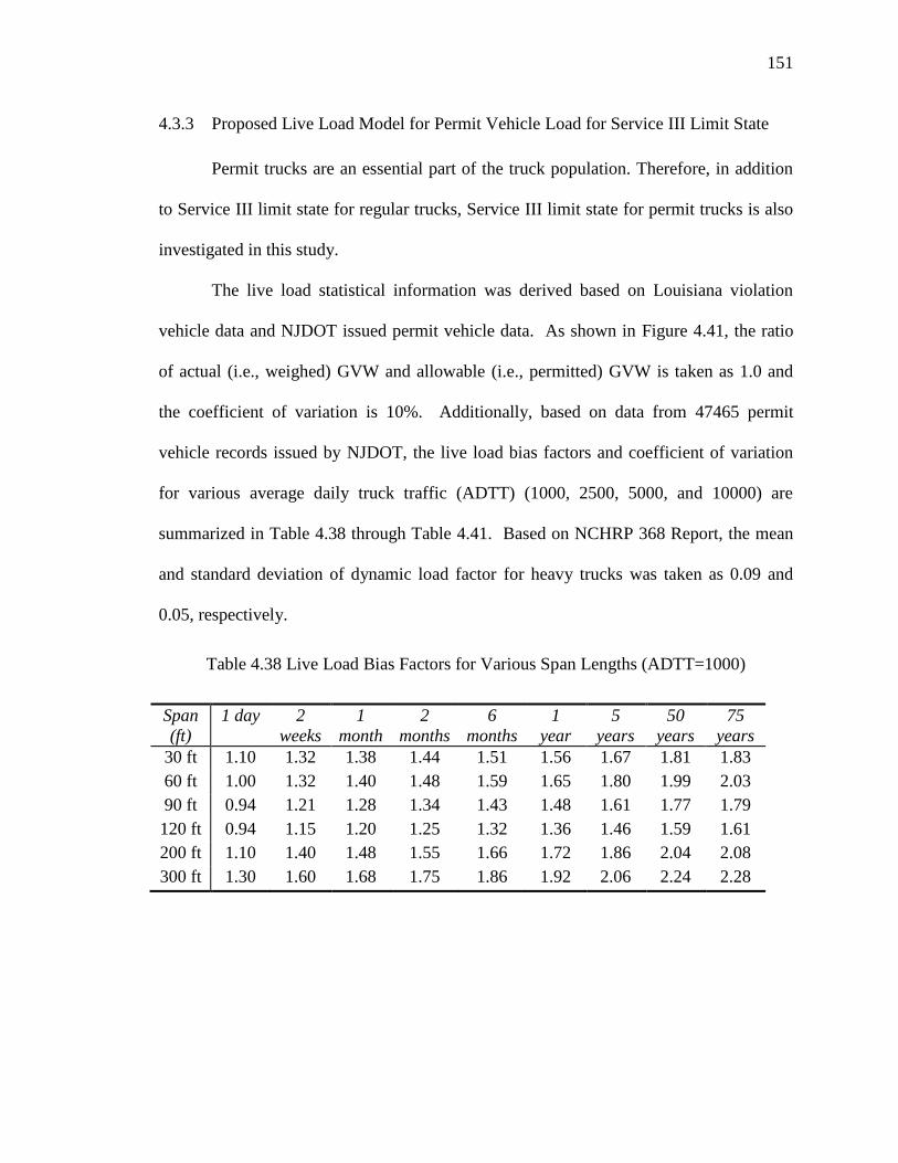
151
4.3.3 Proposed Live Load Model for Permit Vehicle Load for Service III Limit State
Permit trucks are an essential part of the truck population. Therefore, in addition
to Service III limit state for regular trucks, Service III limit state for permit trucks is also
investigated in this study.
The live load statistical information was derived based on Louisiana violation
vehicle data and NJDOT issued permit vehicle data. As shown in Figure 4.41, the ratio
of actual (i.e., weighed) GVW and allowable (i.e., permitted) GVW is taken as 1.0 and
the coefficient of variation is 10%. Additionally, based on data from 47465 permit
vehicle records issued by NJDOT, the live load bias factors and coefficient of variation
for various average daily truck traffic (ADTT) (1000, 2500, 5000, and 10000) are
summarized in Table 4.38 through Table 4.41. Based on NCHRP 368 Report, the mean
and standard deviation of dynamic load factor for heavy trucks was taken as 0.09 and
0.05, respectively.
Table 4.38 Live Load Bias Factors for Various Span Lengths (ADTT=1000)
Span
(ft)
1 day 2
weeks
1
month
2
months
6
months
1
year
5
years
50
years
75
years
30 ft 1.10 1.32 1.38 1.44 1.51 1.56 1.67 1.81 1.83
60 ft 1.00 1.32 1.40 1.48 1.59 1.65 1.80 1.99 2.03
90 ft 0.94 1.21 1.28 1.34 1.43 1.48 1.61 1.77 1.79
120 ft 0.94 1.15 1.20 1.25 1.32 1.36 1.46 1.59 1.61
200 ft 1.10 1.40 1.48 1.55 1.66 1.72 1.86 2.04 2.08
300 ft 1.30 1.60 1.68 1.75 1.86 1.92 2.06 2.24 2.28
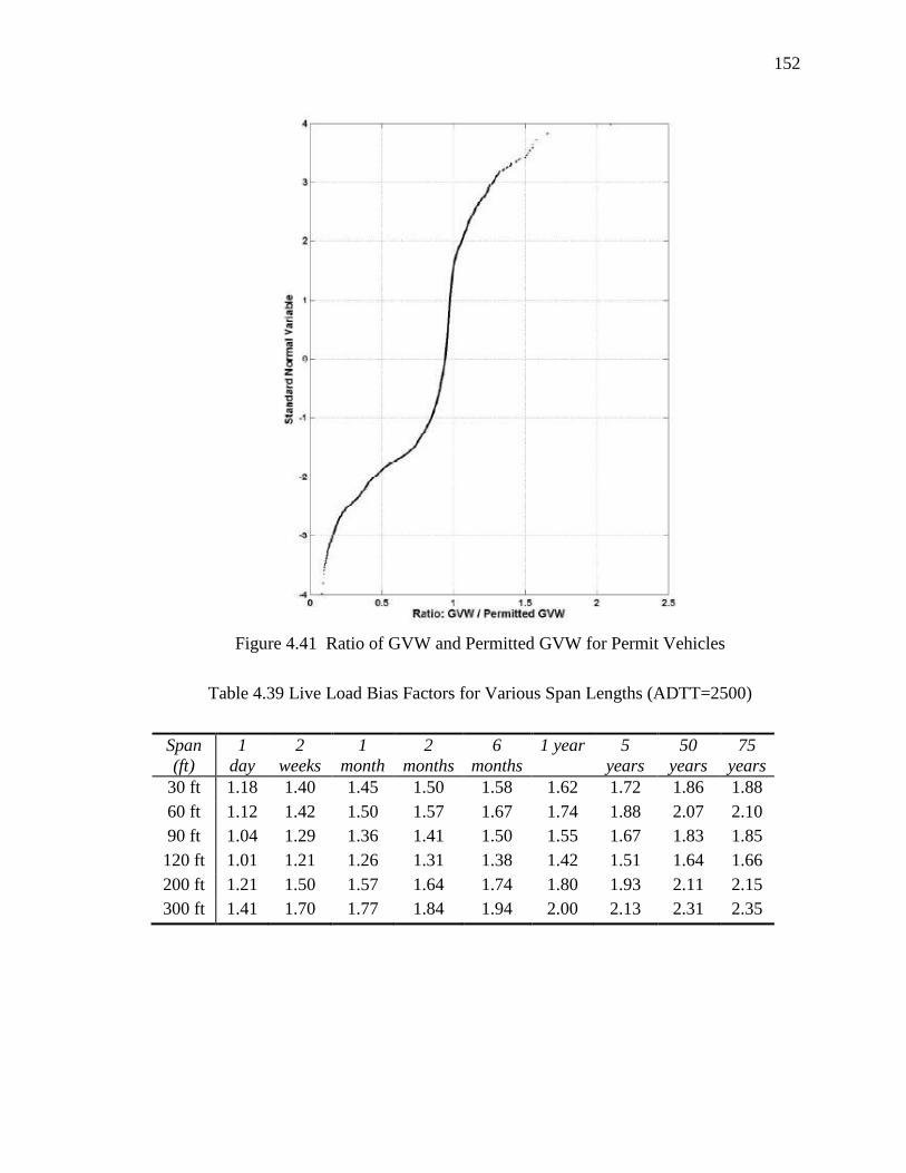
152
Figure 4.41 Ratio of GVW and Permitted GVW for Permit Vehicles
Table 4.39 Live Load Bias Factors for Various Span Lengths (ADTT=2500)
Span
(ft)
1
day
2
weeks
1
month
2
months
6
months
1 year 5
years
50
years
75
years
30 ft 1.18 1.40 1.45 1.50 1.58 1.62 1.72 1.86 1.88
60 ft 1.12 1.42 1.50 1.57 1.67 1.74 1.88 2.07 2.10
90 ft 1.04 1.29 1.36 1.41 1.50 1.55 1.67 1.83 1.85
120 ft 1.01 1.21 1.26 1.31 1.38 1.42 1.51 1.64 1.66
200 ft 1.21 1.50 1.57 1.64 1.74 1.80 1.93 2.11 2.15
300 ft 1.41 1.70 1.77 1.84 1.94 2.00 2.13 2.31 2.35
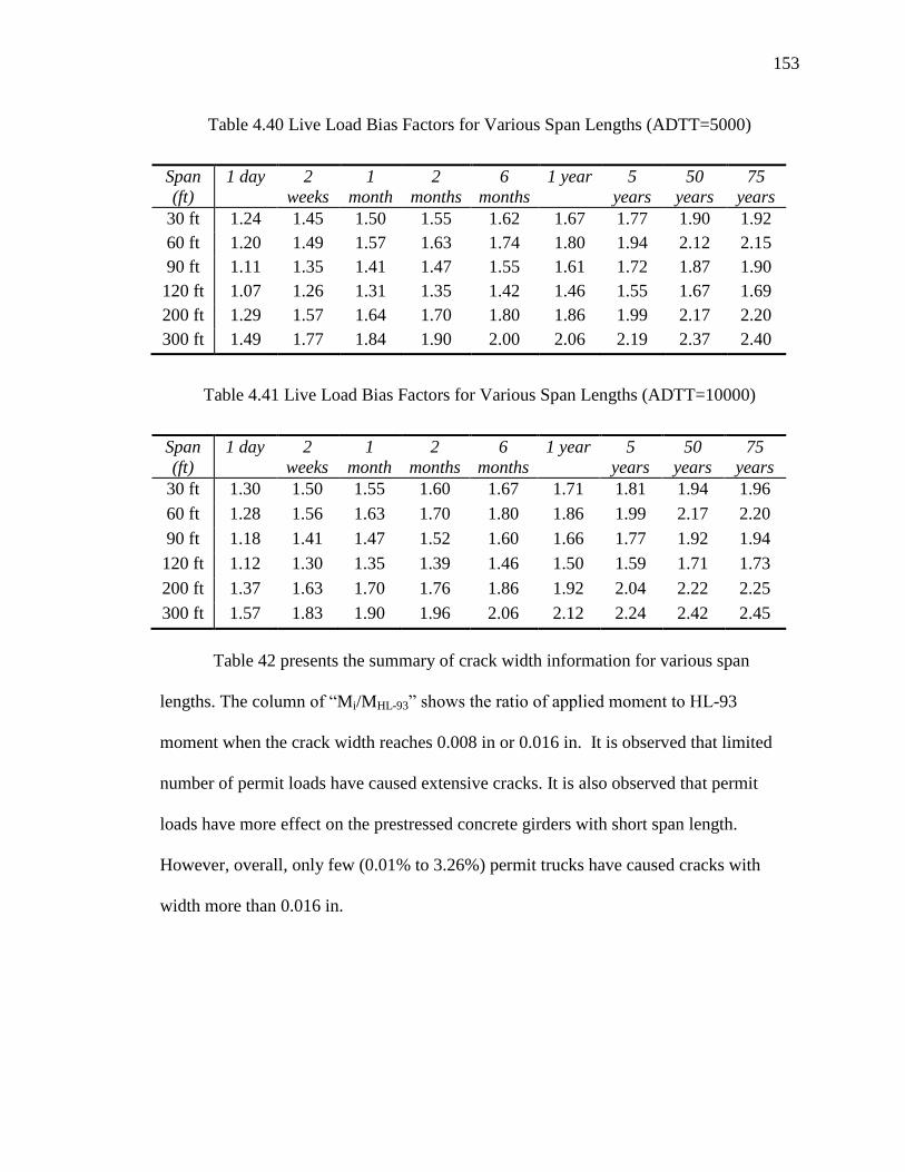
153
Table 4.40 Live Load Bias Factors for Various Span Lengths (ADTT=5000)
Span
(ft)
1 day 2
weeks
1
month
2
months
6
months
1 year 5
years
50
years
75
years
30 ft 1.24 1.45 1.50 1.55 1.62 1.67 1.77 1.90 1.92
60 ft 1.20 1.49 1.57 1.63 1.74 1.80 1.94 2.12 2.15
90 ft 1.11 1.35 1.41 1.47 1.55 1.61 1.72 1.87 1.90
120 ft 1.07 1.26 1.31 1.35 1.42 1.46 1.55 1.67 1.69
200 ft 1.29 1.57 1.64 1.70 1.80 1.86 1.99 2.17 2.20
300 ft 1.49 1.77 1.84 1.90 2.00 2.06 2.19 2.37 2.40
Table 4.41 Live Load Bias Factors for Various Span Lengths (ADTT=10000)
Span
(ft)
1 day 2
weeks
1
month
2
months
6
months
1 year 5
years
50
years
75
years
30 ft 1.30 1.50 1.55 1.60 1.67 1.71 1.81 1.94 1.96
60 ft 1.28 1.56 1.63 1.70 1.80 1.86 1.99 2.17 2.20
90 ft 1.18 1.41 1.47 1.52 1.60 1.66 1.77 1.92 1.94
120 ft 1.12 1.30 1.35 1.39 1.46 1.50 1.59 1.71 1.73
200 ft 1.37 1.63 1.70 1.76 1.86 1.92 2.04 2.22 2.25
300 ft 1.57 1.83 1.90 1.96 2.06 2.12 2.24 2.42 2.45
Table 42 presents the summary of crack width information for various span
lengths. The column of “Mi/MHL-93” shows the ratio of applied moment to HL-93
moment when the crack width reaches 0.008 in or 0.016 in. It is observed that limited
number of permit loads have caused extensive cracks. It is also observed that permit
loads have more effect on the prestressed concrete girders with short span length.
However, overall, only few (0.01% to 3.26%) permit trucks have caused cracks with
width more than 0.016 in.
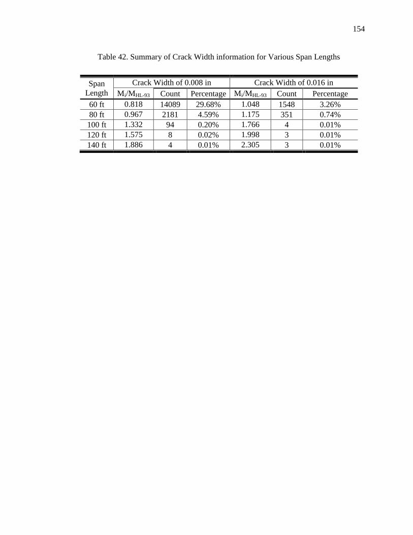
154
Table 42. Summary of Crack Width information for Various Span Lengths
Span
Length
Crack Width of 0.008 in Crack Width of 0.016 in
Mi/MHL-93 Count Percentage Mi/MHL-93 Count Percentage
60 ft 0.818 14089 29.68% 1.048 1548 3.26%
80 ft 0.967 2181 4.59% 1.175 351 0.74%
100 ft 1.332 94 0.20% 1.766 4 0.01%
120 ft 1.575 8 0.02% 1.998 3 0.01%
140 ft 1.886 4 0.01% 2.305 3 0.01%

155
5 DETERIORATION MODEL OF BRIDGE ELEMENTS
CHAPTER 5
DETERIORATION MODEL OF BRIDGE ELEMENTS
As more and more infrastructures are approaching the limit of their service life,
the deterioration of structure gains more attention from the owner, user, as well as
designers and engineers. However, current design specifications do not integrate the
deterioration of structure into design process. During the calibration of AASHTO LRFD
Design Specification for ultimate limit state, the long term effect of live load was
considered by extrapolating to different return periods including 75 years. However, the
deterioration of the resistance capacity was not included. Thus, it is needed to evaluate
the structural deterioration on reliability of structures.
There are two most common causes of deterioration of concrete structures:
Freezing-Thaw and corrosion of steel caused by chloride penetration. The deterioration
of structure can be divided into two categories: deterioration of section and deterioration
of strength. In this study, the time dependent properties of section and strength were
investigated and discussed. Hereafter the deterioration models for structural resistance
were developed for reinforced concrete decks at Service I limit state and prestressed
concrete girders at Service III limit state. These deterioration models will be used in the
reliability analysis in Chapter 6.

156
5.1 Deterioration Model for Prestressed Concrete Girders for Service III Limit
State
Although overall prestressed concrete girder bridges have demonstrated good
performance in adverse exposure conditions, due to extensive chlorides and moisture,
tendon failures were found in several post-tensioned concrete girder bridges, such as
Niles Channel, Mid-bay, and Bob Graham Sunshine Skyway bridges in Florida (FDOT,
1999, 2001a, and 2001
b) and Varina-Enon Bridge in Virginia (Hansen 2007). Therefore,
an appropriate deterioration model could help to better understand the effect of
deterioration of reliability and serviceability of structure.
The deterioration of prestressed concrete girders contains three major
components: time-variant of concrete strength, losses of concrete section, and strength
losses in prestressing strands. Since the losses of concrete section has not been fully
studied and minor loss of concrete section has no significant effect on the resistance of
the structure, only time-variant property of concrete strength and strength losses in
prestressing strands were considered in this study.
Due to the shrinkage and creep effects over time, the strength of concrete varies.
The prediction equation developed by ACI Committee 209 is adopted in this study:
28( ') ( ')c t c
tf f
a t
Eq. 5.1
where,
a = Empirical constant depends on the cement type and curing method
= Empirical constant depends on the cement type and curing method
t = Age of concrete in days

157
28( ')cf = 28-day compressive strength of concrete
( ')c tf = Compressive strength of concrete at age of t.
The ultimate tensile strength of prestressing tendons for post-tensioned concrete
girder at long term is predicted using the equation developed by Pillai, et. al (2010) as
shown below:
1 3 4 %( ) ln( )pu t pu tWD tWDsCl
f f h h h
Eq. 5.2
where,
i = Model parameters, 1 =0.9463, 2 =1.0333, 3 =0.3567, and 4 =0.0285.
puf = Ultimate strength of prestressing tendon
( )pu tf = Ultimate strength of prestressing tendon in t years
tWDh = 12( )
Wet timeina yearTotal years
months
%sClh =
%Cl inthe water insidethetendon
Saturated Chloride Solution
= Standard deviation of model error, 0.0350
= Standard normal Variable~Normal (0,1)
The long term losses of prestressing strength ( pSDf + pCDf + pR2f - pSSf ) after
deck placement are predicted using the provisions in AASHTO LRFD Bridge Design
Specification 2012, as shown below:
Due to Shrinkage of Girder Concrete
dfpbdfpSD KEf Eq. 5.3

158
for which:
)0.7(1I
eA1
A
A
E
E1
1K
bif
c
2
pcc
c
ps
ci
p
df
Eq. 5.4
where:
pSDf = prestress loss due to shrinkage of girder concrete between time of deck
placement and final time
bdf = shrinkage strain of girder between time of deck placement and final time
Kdf = transformed section coefficient that accounts for time-dependent
interaction between concrete and bonded steel in the section being
considered for time period between deck placement and final time
epc = eccentricity of strands with respect to centroid of composite section
Ac = area of composite section calculated using the gross concrete section
properties of the girder and the deck and the deck-to-girder modular ratio
Ic = moment of inertia of composite section calculated using the gross
concrete section properties of the girder and the deck and the deck-to-
girder modular ratio at service
Due to Creep of Girder Concrete:
0.0KfE
E)K(f
E
Ef dfbdfcd
c
p
dfbidbifcgp
ci
p
pCD Eq. 5.5
where:
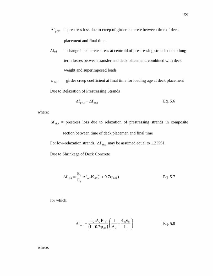
159
pCDf = prestress loss due to creep of girder concrete between time of deck
placement and final time
fcd = change in concrete stress at centroid of prestressing strands due to long-
term losses between transfer and deck placement, combined with deck
weight and superimposed loads
bdf = girder creep coefficient at final time for loading age at deck placement
Due to Relaxation of Prestressing Strands
pR2pR3 ff Eq. 5.6
where:
3pRf = prestress loss due to relaxation of prestressing strands in composite
section between time of deck placemen and final time
For low-relaxation strands, 2pRf may be assumed equal to 1.2 KSI
Due to Shrinkage of Deck Concrete
)0.7(1KfE
Ef bdfdfcdf
c
p
pSS Eq. 5.7
for which:
df
cddddfcdf
0.71
EAf
c
dpc
c I
ee
A
1 Eq. 5.8
where:
160
pSSf = prestress loss due to shrinkage of deck composite section
cdff = change in concrete stress at centroid of prestressing strands due to
shrinkage of deck concrete
ddf = shrinkage strain of deck concrete between placement and final time
Ad = area of deck concrete
Ecd = modulus of elasticity of deck concrete
ed = eccentricity of deck with respect to the transformed composite section,
taken negative in common construction
df = creep coefficient of deck concrete at final time due to loading
introduced shortly after deck placement.(i.e. overlays, barriers, etc.)
Therefore, the effective stress of prestressing tendon, ( )se tf , can be calculated
using the following equation:
( ) ( ) ( )se t si si st si ltf f f f Eq. 5.9
where,
sif = initial prestressing stress
( )si stf = short term prestressing losses
( )si ltf = long term prestressing losses, ( )si ltf = pSDf + pCDf + pR2f - pSSf
The researchers have found that the corrosion of steel would affect the area of
steel but not the local ultimate strength of steel (Hanjari (2010), Darmawan and Stewart
(2007), and Almusallam (2001)). As shown in Figure 5.1, the degree of corrosion has
little effect on ultimate strength of bar.
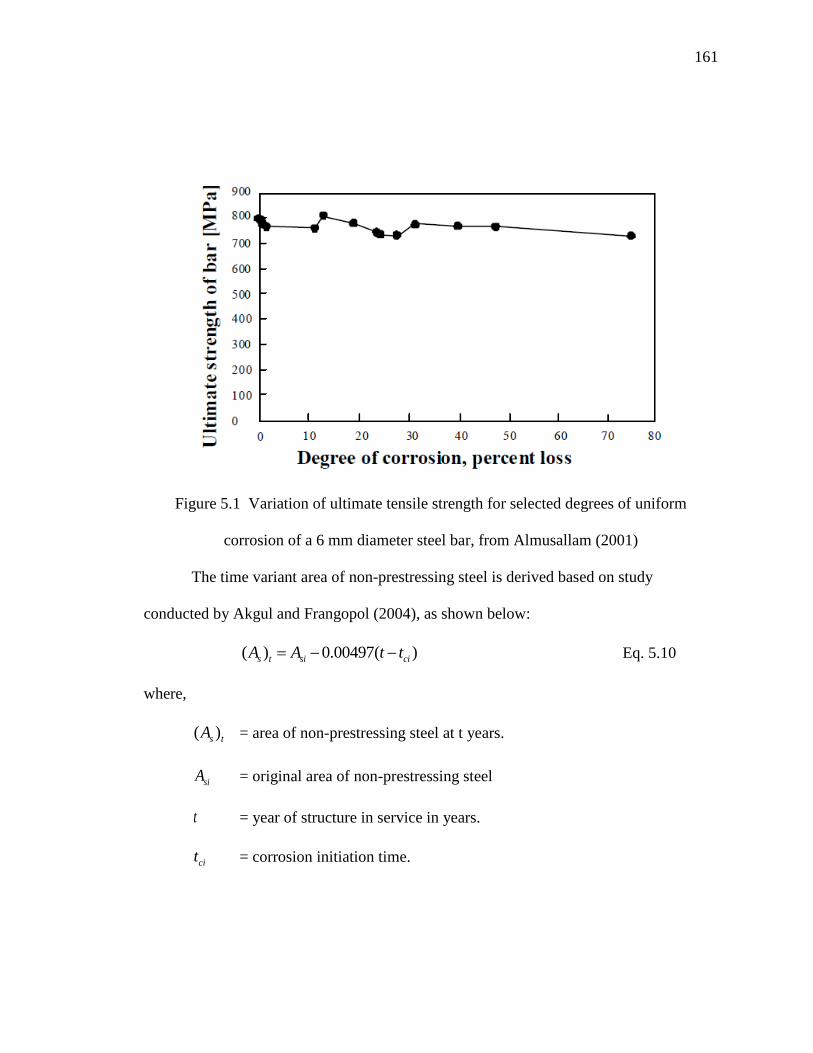
161
Figure 5.1 Variation of ultimate tensile strength for selected degrees of uniform
corrosion of a 6 mm diameter steel bar, from Almusallam (2001)
The time variant area of non-prestressing steel is derived based on study
conducted by Akgul and Frangopol (2004), as shown below:
( ) 0.00497( )s t si ciA A t t Eq. 5.10
where,
( )s tA = area of non-prestressing steel at t years.
siA = original area of non-prestressing steel
t = year of structure in service in years.
cit = corrosion initiation time.
162
Therefore, applying all the time variant parameters, the deterioration model of
resistance for prestressed concrete girders at Service III limit state can be expressed as
formula below:
2
02
1 2 0
( ) ( ) 21(( ) ( ) ) ( ) ( )
6 2 3
f f
n ps pu t ps t ps p s t s s ct ct
c h b b c hM A f f f d A f d f b c f
c
2
1 1( ) ( ) 2 2( )
2 3
f f w f f
ct
c h h b b c h hf
c
Eq. 5.11
where,
( )s tA = area of non-prestressing steel at t years.
1( )ps tf = prestress losses at t years after prestressing.
2psf = change of stress in prestressing tendons after applying live load.
5.2 Deterioration Model for Reinforced Concrete Decks at Service I Limit State
Similar to deterioration model for prestressed concrete girders at Service III limit
state, utilizing the time variant parameters listed in section 5.1, the deterioration model
for resistance of reinforced concrete decks designed using empirical design method at
Service I limit state can be expressed as:
2
2
2 2 ' 2
1
22
3 ( ) 3 ( ) 2( ) 0.85
(4( ) 9 )( ) 4
c ss
c
s t s c s t s s t s c r c t
s t s c s t
w Ef
sd
A E E bd A E A E E bd M f d
d A E E bd A
Eq. 5.12

163
Although the resistance model for reinforced concrete decks designed using
traditional design method does not involve any time variant parameters, the time variant
parameters are included in the limit state function when calculating the stress due to the
live load. Therefore, the deterioration of the concrete and steel will still be considered in
the reliability analysis presented in section 6.1.5.
164
6 STRUCTURAL RELIABILTY ANALYSIS
CHAPTER 6
STRUCTURAL RELIABILITY ANALYSIS
Structural reliability analysis method is a rational, probability based approach to
identify the safety or probability of failure of a structure at various limit states. The term
limit state is used to define the boundary between “success” and “failure” for various
aspects of structural performance. The limit state is usually expressed as a function
with random variables . Mathematically, if is greater than 0,
the structure is safe. If is less than 0, the structure is failed for this limit state. The
limit state can be used to represent various performance criteria in structural engineering.
These performance criteria or limit state can be categorized into three main categories:
ultimate, serviceability, and fatigue. Ultimate limit states are the limit states that
represent the ultimate capacity of the structure in terms of flexure, shear, torsion, or
buckling. The failure of ultimate limit state such as exceeding of the moment carrying
capacity of the structure, crashing of concrete in compression, or buckling of the web is
fatal to the structure and will result in unrecovered damage if the limit state is violated. In
contrast, serviceability limit states are the limit states covers various aspects of
serviceability of structure such as cracking, deflection, vibration, etc. Failure of
serviceability limit states might not result in catastrophic consequences directly.
However, Serviceability limit states related to stress, deformation, and crack under
regular service conditions are essential to the performance, human experience, and
165
durability of structure. Finally, fatigue limit states are the limit states that related to the
deterioration and damage of the structure under repeated loading. Failure of fatigue limit
states can be occurrence of fatigue cracks, high stresses in secondary members, and
damage to welded connections. The term “failure” is an expression of exceedance of limit
state and the consequence of failure varies depending on the limit state.
Due to the nature of the limit state which always composes two basic variables,
resistance and load, the limit state function is expressed as:
Eq. 6.1
where R represents the resistance of the structure and Q represents the load effect
that relates to the specific limit state. The limit state boundary is defined as a scenario
whereby the resistance is numerically equal to the load effects, and is expressed by g = 0.
When the resistance exceeds the load effect, R>Q, the structure is safe, otherwise the
limit state is violated.
In previous sections, the resistance models and live load models were developed
for various serviceability limit states. Moreover, the deterioration models were also
developed for structural resistance in Chapter 5. In this Chapter, the limit state will be
formulated and the structural reliability analysis procedure will be assembled for each
serviceability limit state. Applying the resistance models, load models, and deterioration
models developed in previous Chapters, structural reliability analysis will be performed
and target reliability indices will be proposed hereafter for each serviceability limit state.
Then various design provisions will be modified to improve the level and uniformity of
reliability for each limit state. In addition, the effect of structural deterioration on
reliability of structure will be evaluated.
166
6.1 Reinforced Concrete Decks Designed using Traditional Method (Service I
Limit State)
In this section, utilizing the resistance model and load model developed in previous
Chapters, the structural analysis will be performed for reinforced concrete decks designed
using traditional method for Service I limit state. Section 6.1.1 shows the representative
data base used in this study. Section 6.1.2 shows the assembled limit state function.
Section 6.1.3 shows the reliably index of current practice and proposed target reliability
index for this limit state. Section 6.1.4 shows reliability analysis results of various
scenarios by changing design provisions. Finally, section 6.1.5 presents the effect of
structural deterioration on reliability of reinforced concrete deck at Service I limit state.
6.1.1 Reinforced Concrete Deck Database
A set of reinforced concrete decks was designed using traditional equivalent strip
method based on AASHTO LRFD Bridge Design Specification. These designed bridge
decks covered various girder spacing and deck thickness. Table 6.1 presents the
summary information of 15 designed bridge decks. This set of bridge decks will be used
as a representative database in this study.
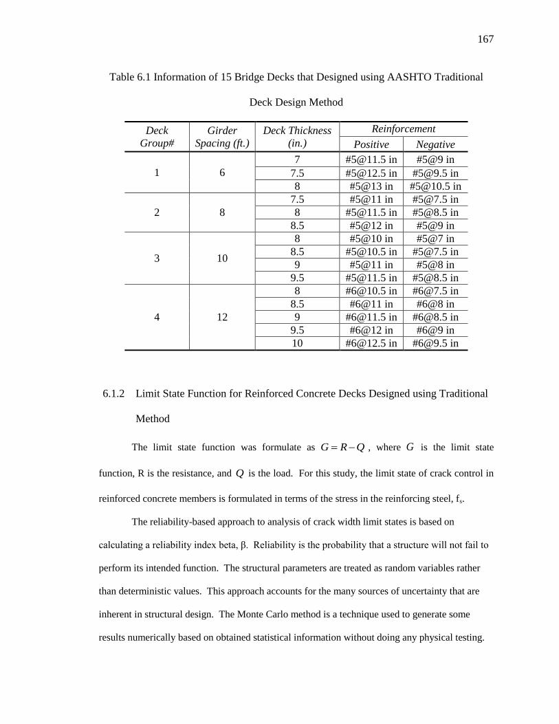
167
Table 6.1 Information of 15 Bridge Decks that Designed using AASHTO Traditional
Deck Design Method
Deck
Group#
Girder
Spacing (ft.)
Deck Thickness
(in.)
Reinforcement
Pos. Neg. Positive Negative
1 6
7 #[email protected] in #5@9 in
7.5 #[email protected] in #[email protected] in
8 #5@13 in #[email protected] in
2 8
7.5 #5@11 in #[email protected] in
8 #[email protected] in #[email protected] in
8.5 #5@12 in #5@9 in
3 10
8 #5@10 in #5@7 in
8.5 #[email protected] in #[email protected] in
9 #5@11 in #5@8 in
9.5 #[email protected] in #[email protected] in
4 12
8 #[email protected] in #[email protected] in
8.5 #6@11 in #6@8 in
9 #[email protected] in #[email protected] in
9.5 #6@12 in #6@9 in
10 #[email protected] in #[email protected] in
6.1.2 Limit State Function for Reinforced Concrete Decks Designed using Traditional
Method
The limit state function was formulate as G R Q , where G is the limit state
function, R is the resistance, and Q is the load. For this study, the limit state of crack control in
reinforced concrete members is formulated in terms of the stress in the reinforcing steel, fs.
The reliability-based approach to analysis of crack width limit states is based on
calculating a reliability index beta, β. Reliability is the probability that a structure will not fail to
perform its intended function. The structural parameters are treated as random variables rather
than deterministic values. This approach accounts for the many sources of uncertainty that are
inherent in structural design. The Monte Carlo method is a technique used to generate some
results numerically based on obtained statistical information without doing any physical testing.

168
The reliability index, β, is based on the mean and standard deviation of a limit state function, G,
which is defined as G = R-Q. The Monte Carlo method, β = μG/σG where μG = mean of the
function G and σG = standard deviation of the function G.
To approach crack width limit states using the reliability approach, the function G will be
written in terms of the steel reinforcement stress, fs, since research has shown this to be the most
important parameter influencing crack widths. Moreover, the steel stress can be obtained directly
from the applied load using equilibrium equation and strain compatibility. Thus, the limit state
function would appear as such:
(resistance) (load)s sG f f Eq. 6.2
The resistance R was derived as shown in section 3.1. The load, Q, in the reliability
approach was derived based on principles of reinforced concrete analysis. Force and moment
equilibrium were used to solve for two unknowns: 1) steel stress, fs, and 2) depth of the neutral
axis, Cna. The maximum moment is calculated based on HL-93 loading and the moment
resistance is / 3s s naA f d C where sA is the area of steel reinforcement and fy is the yield
stress of the steel.
From force equilibrium and assuming linear concrete stress distribution, the compression
force for a beam with rectangular section having a width b and depth d, is calculated as
follows:
2 2
c na c c nac
f C b E C bC
Eq. 6.3
Moreover, assuming linear elastic behavior, the tension force carried by the steel
reinforcement can be calculated as follows:
s s s s sT A f A E Eq. 6.4

169
Using the force and moment equilibrium equations to solve for fs the following equation is
obtained:
2 2
max3 3 2
(4 9 )
s s c s s s s c
s
s s c s
A E E bd A E A E E bd Mf
d A E E bd A
Eq. 6.5
where:
sA = area of steel reinforcement, in2
sE = elastic modulus of steel, psi
cE = elastic modulus of concrete, psi
b = width of concrete section, in
d = effective depth of concrete section, in
P = applied load, lbs
L = span length, in
maxM = The maximum live load moment due to HL-93 Loading.
Thus, the limit state function, G R Q , can be written as follows:
2 2
max
2
2
3 3 2
(4 9 )2
2
s s c s s s s cc s
s s c s
c
A E E bd A E A E E bd Mw EG
d A E E bd Asd
Eq. 6.6
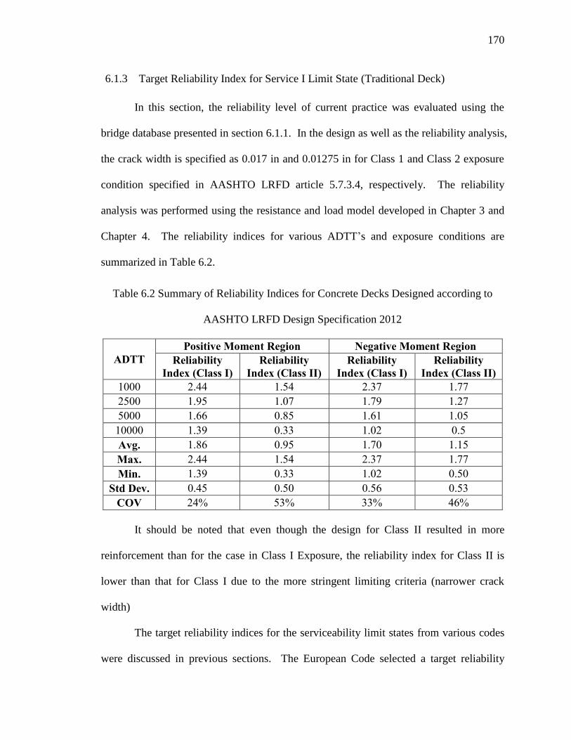
170
6.1.3 Target Reliability Index for Service I Limit State (Traditional Deck)
In this section, the reliability level of current practice was evaluated using the
bridge database presented in section 6.1.1. In the design as well as the reliability analysis,
the crack width is specified as 0.017 in and 0.01275 in for Class 1 and Class 2 exposure
condition specified in AASHTO LRFD article 5.7.3.4, respectively. The reliability
analysis was performed using the resistance and load model developed in Chapter 3 and
Chapter 4. The reliability indices for various ADTT’s and exposure conditions are
summarized in Table 6.2.
Table 6.2 Summary of Reliability Indices for Concrete Decks Designed according to
AASHTO LRFD Design Specification 2012
ADTT
Positive Moment Region Negative Moment Region
Reliability
Index (Class I)
Reliability
Index (Class II)
Reliability
Index (Class I)
Reliability
Index (Class II)
1000 2.44 1.54 2.37 1.77
2500 1.95 1.07 1.79 1.27
5000 1.66 0.85 1.61 1.05
10000 1.39 0.33 1.02 0.5
Avg. 1.86 0.95 1.70 1.15
Max. 2.44 1.54 2.37 1.77
Min. 1.39 0.33 1.02 0.50
Std Dev. 0.45 0.50 0.56 0.53
COV 24% 53% 33% 46%
It should be noted that even though the design for Class II resulted in more
reinforcement than for the case in Class I Exposure, the reliability index for Class II is
lower than that for Class I due to the more stringent limiting criteria (narrower crack
width)
The target reliability indices for the serviceability limit states from various codes
were discussed in previous sections. The European Code selected a target reliability
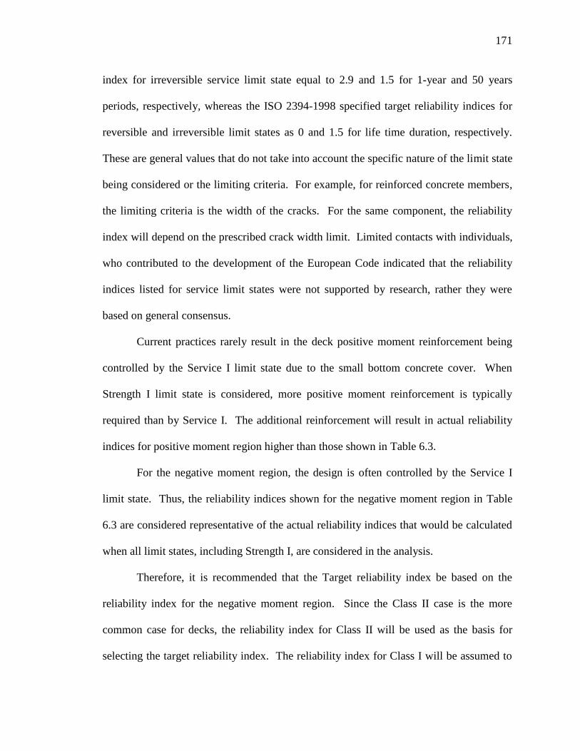
171
index for irreversible service limit state equal to 2.9 and 1.5 for 1-year and 50 years
periods, respectively, whereas the ISO 2394-1998 specified target reliability indices for
reversible and irreversible limit states as 0 and 1.5 for life time duration, respectively.
These are general values that do not take into account the specific nature of the limit state
being considered or the limiting criteria. For example, for reinforced concrete members,
the limiting criteria is the width of the cracks. For the same component, the reliability
index will depend on the prescribed crack width limit. Limited contacts with individuals,
who contributed to the development of the European Code indicated that the reliability
indices listed for service limit states were not supported by research, rather they were
based on general consensus.
Current practices rarely result in the deck positive moment reinforcement being
controlled by the Service I limit state due to the small bottom concrete cover. When
Strength I limit state is considered, more positive moment reinforcement is typically
required than by Service I. The additional reinforcement will result in actual reliability
indices for positive moment region higher than those shown in Table 6.3.
For the negative moment region, the design is often controlled by the Service I
limit state. Thus, the reliability indices shown for the negative moment region in Table
6.3 are considered representative of the actual reliability indices that would be calculated
when all limit states, including Strength I, are considered in the analysis.
Therefore, it is recommended that the Target reliability index be based on the
reliability index for the negative moment region. Since the Class II case is the more
common case for decks, the reliability index for Class II will be used as the basis for
selecting the target reliability index. The reliability index for Class I will be assumed to

172
represent relaxation of the base requirements. Table 6.3 shows the inherent and proposed
target reliability indices for the negative moment region of decks designed for the current
AASHTO LRFD Specifications.
Table 6.3 Reliability Indices of Existing Bridges based on 1-year return period
ADTT
Reliability Index
Current Practice
(Class I, Negative)
Current Practice
(Class II, Negative)
Target β (Class I,
Negative)
Target β (Class II,
Negative)
1000 2.37 1.77
1.6
1.0
2500 1.79 1.27
5000 1.61 1.05
10,000 1.02 0.50
6.1.4 Reliability analysis results for Service I Limit State
6.1.4.1 Class 1 Exposure Condition (Maximum Crack Width of 0.017 in)
Figure 6.1 and Figure 6.2 present the reliability indices for various bridge decks designed
using a live load factor of 1.0 over one year period, which reflected the reliability level of
current design. It can be observed that the average reliability index is around 2.44 and
2.37 for positive and negative moment regions, respectively.
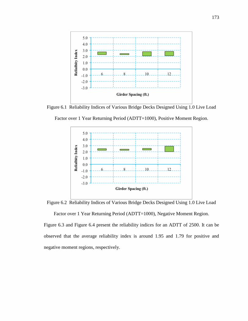
173
Figure 6.1 Reliability Indices of Various Bridge Decks Designed Using 1.0 Live Load
Factor over 1 Year Returning Period (ADTT=1000), Positive Moment Region.
Figure 6.2 Reliability Indices of Various Bridge Decks Designed Using 1.0 Live Load
Factor over 1 Year Returning Period (ADTT=1000), Negative Moment Region.
Figure 6.3 and Figure 6.4 present the reliability indices for an ADTT of 2500. It can be
observed that the average reliability index is around 1.95 and 1.79 for positive and
negative moment regions, respectively.
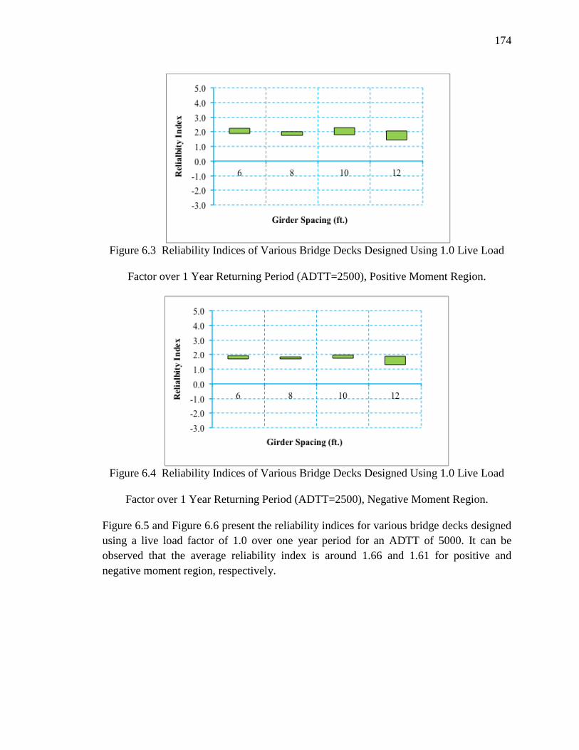
174
Figure 6.3 Reliability Indices of Various Bridge Decks Designed Using 1.0 Live Load
Factor over 1 Year Returning Period (ADTT=2500), Positive Moment Region.
Figure 6.4 Reliability Indices of Various Bridge Decks Designed Using 1.0 Live Load
Factor over 1 Year Returning Period (ADTT=2500), Negative Moment Region.
Figure 6.5 and Figure 6.6 present the reliability indices for various bridge decks designed
using a live load factor of 1.0 over one year period for an ADTT of 5000. It can be
observed that the average reliability index is around 1.66 and 1.61 for positive and
negative moment region, respectively.
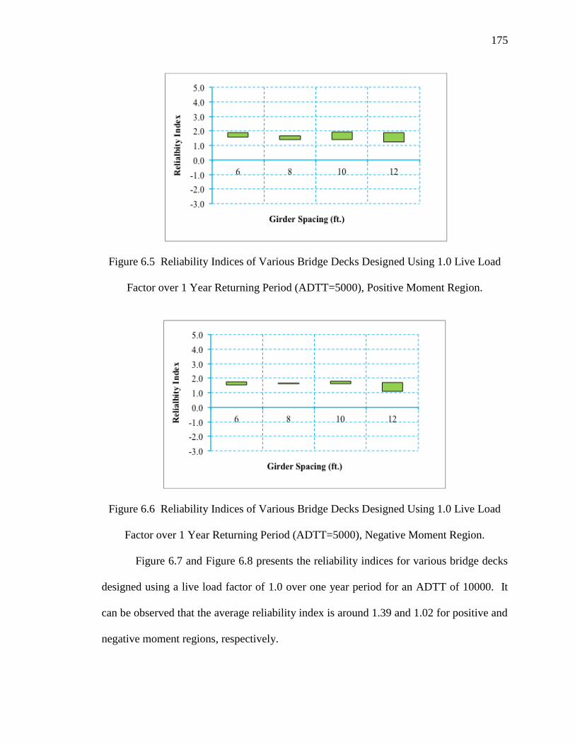
175
Figure 6.5 Reliability Indices of Various Bridge Decks Designed Using 1.0 Live Load
Factor over 1 Year Returning Period (ADTT=5000), Positive Moment Region.
Figure 6.6 Reliability Indices of Various Bridge Decks Designed Using 1.0 Live Load
Factor over 1 Year Returning Period (ADTT=5000), Negative Moment Region.
Figure 6.7 and Figure 6.8 presents the reliability indices for various bridge decks
designed using a live load factor of 1.0 over one year period for an ADTT of 10000. It
can be observed that the average reliability index is around 1.39 and 1.02 for positive and
negative moment regions, respectively.
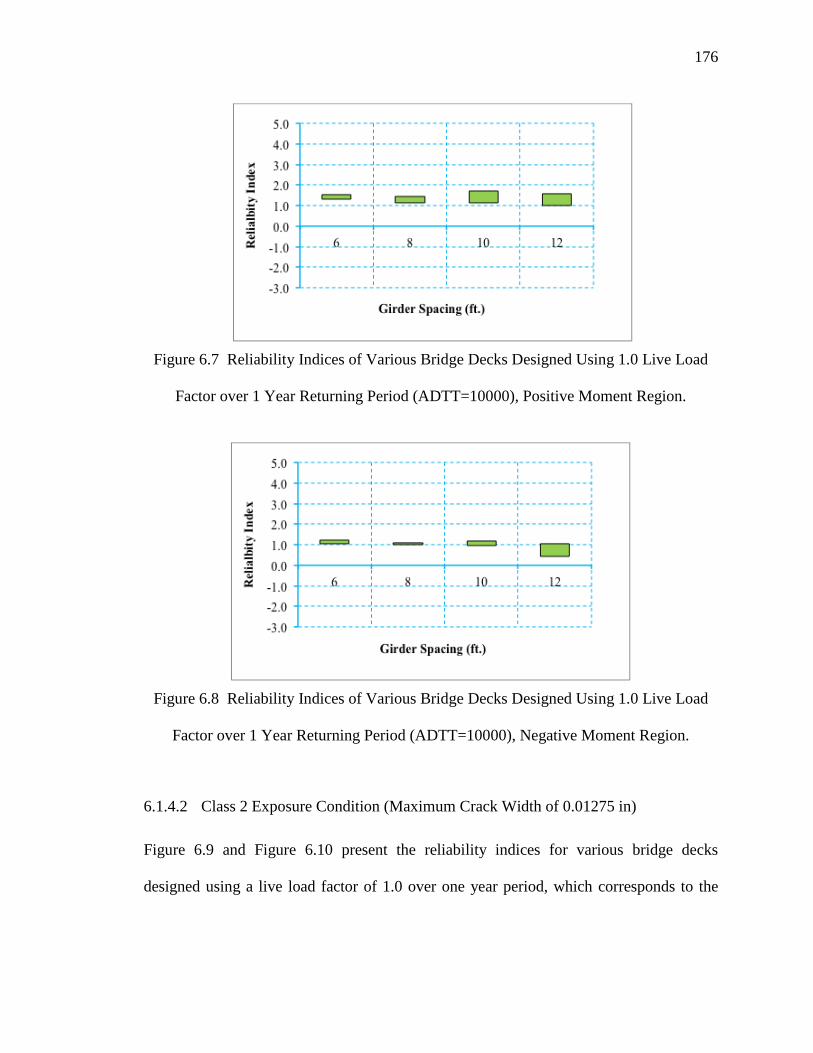
176
Figure 6.7 Reliability Indices of Various Bridge Decks Designed Using 1.0 Live Load
Factor over 1 Year Returning Period (ADTT=10000), Positive Moment Region.
Figure 6.8 Reliability Indices of Various Bridge Decks Designed Using 1.0 Live Load
Factor over 1 Year Returning Period (ADTT=10000), Negative Moment Region.
6.1.4.2 Class 2 Exposure Condition (Maximum Crack Width of 0.01275 in)
Figure 6.9 and Figure 6.10 present the reliability indices for various bridge decks
designed using a live load factor of 1.0 over one year period, which corresponds to the
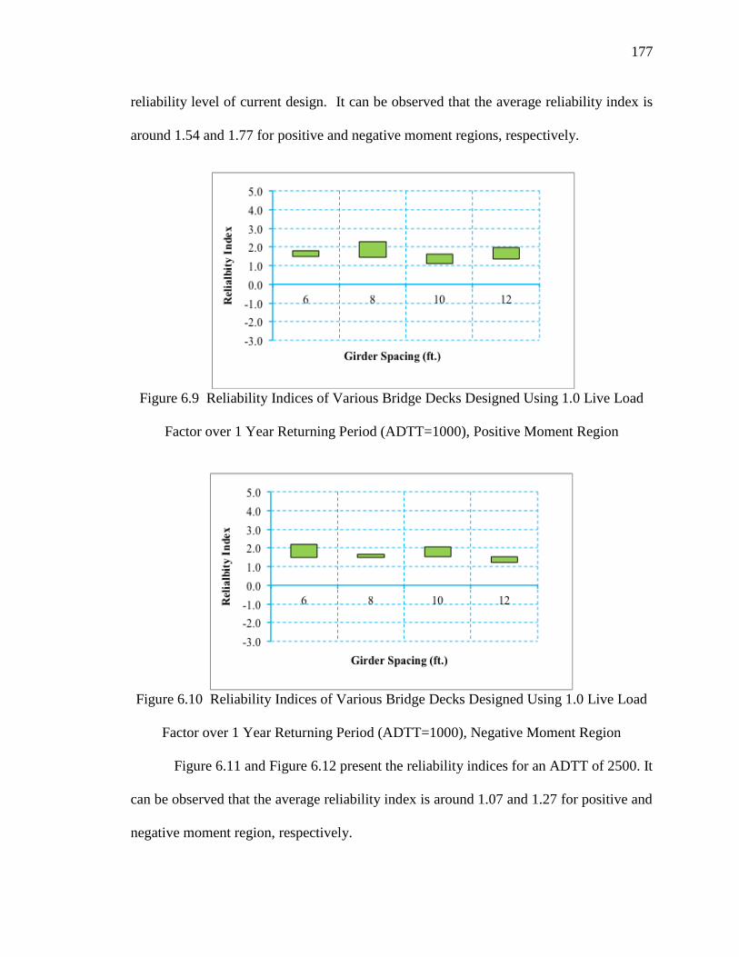
177
reliability level of current design. It can be observed that the average reliability index is
around 1.54 and 1.77 for positive and negative moment regions, respectively.
Figure 6.9 Reliability Indices of Various Bridge Decks Designed Using 1.0 Live Load
Factor over 1 Year Returning Period (ADTT=1000), Positive Moment Region
Figure 6.10 Reliability Indices of Various Bridge Decks Designed Using 1.0 Live Load
Factor over 1 Year Returning Period (ADTT=1000), Negative Moment Region
Figure 6.11 and Figure 6.12 present the reliability indices for an ADTT of 2500. It
can be observed that the average reliability index is around 1.07 and 1.27 for positive and
negative moment region, respectively.

178
Figure 6.11 Reliability Indices of Various Bridge Decks Designed Using 1.0 Live Load
Factor over 1 Year Returning Period (ADTT=2500), Positive Moment Region.
Figure 6.12 Reliability Indices of Various Bridge Decks Designed Using 1.0 Live Load
Factor over 1 Year Returning Period (ADTT=2500), Negative Moment Region.
Figure 6.13 and Figure 6.14 present the reliability indices for various bridge decks
designed using a live load factor of 1.0 over one year period for an ADTT of 5000. It can
be observed that the average reliability index is around 0.85 and 1.05 for positive and
negative moment region, respectively.

179
Figure 6.13 Reliability Indices of Various Bridge Decks Designed Using 1.0 Live Load
Factor over 1 Year Returning Period (ADTT=5000), Positive Moment Region.
Figure 6.14 Reliability Indices of Various Bridge Decks Designed Using 1.0 Live Load
Factor over 1 Year Returning Period (ADTT=5000), Negative Moment Region.
Figure 6.15 and Figure 6.16 present the reliability indices of various bridge decks
designed using a 1.2 live load factor over one year period. It can be observed that the
average reliability index is 1.61 and 2.2 for positive and negative moment regions for 1-
year duration, respectively, which are higher than the target reliability index.
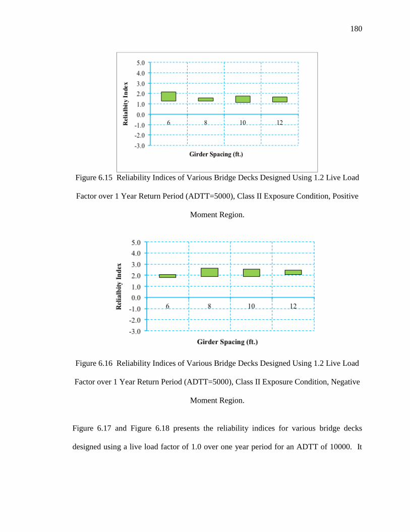
180
Figure 6.15 Reliability Indices of Various Bridge Decks Designed Using 1.2 Live Load
Factor over 1 Year Return Period (ADTT=5000), Class II Exposure Condition, Positive
Moment Region.
Figure 6.16 Reliability Indices of Various Bridge Decks Designed Using 1.2 Live Load
Factor over 1 Year Return Period (ADTT=5000), Class II Exposure Condition, Negative
Moment Region.
Figure 6.17 and Figure 6.18 presents the reliability indices for various bridge decks
designed using a live load factor of 1.0 over one year period for an ADTT of 10000. It
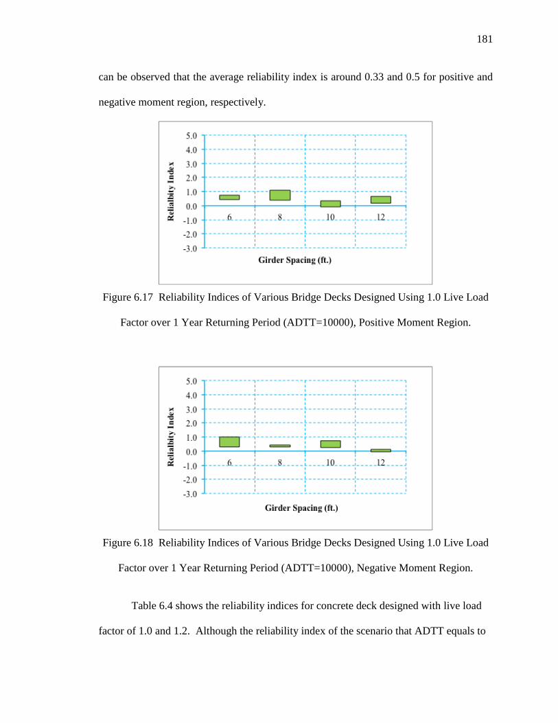
181
can be observed that the average reliability index is around 0.33 and 0.5 for positive and
negative moment region, respectively.
Figure 6.17 Reliability Indices of Various Bridge Decks Designed Using 1.0 Live Load
Factor over 1 Year Returning Period (ADTT=10000), Positive Moment Region.
Figure 6.18 Reliability Indices of Various Bridge Decks Designed Using 1.0 Live Load
Factor over 1 Year Returning Period (ADTT=10000), Negative Moment Region.
Table 6.4 shows the reliability indices for concrete deck designed with live load
factor of 1.0 and 1.2. Although the reliability index of the scenario that ADTT equals to

182
10000 less than the target reliability indices, no revision in AASHTO Specification is
recommended since the current practices satisfy the requirements of target reliability
index for most of the scenarios (ADTT of 1000, 2500, and 5000). Therefore, live load
factor of 1.0 is still being recommended to be used in AASHTO Specification.
Table 6.4 Summary of Reliability Indices for Concrete Decks Designed with Different
Live Load Factors
ADTT
Positive Moment Region Negative Moment Region
Class I Class II Class I Class II
γLL=1.0 γLL=1.0 γLL=1.2 γLL=1.0 γLL=1.0 γLL=1.2
1000 2.44 1.54 2.24 2.37 1.77 2.56
2500 1.95 1.07 1.81 1.79 1.27 2.21
5000 1.66 0.85 1.6 1.61 1.05 2.2
10000 1.39 0.33 1.11 1.02 0.5 1.49
6.1.5 Effects of Structural Deterioration on Reliability of Service I Limit State
(Traditional Deck)
Although the resistance model for reinforced concrete decks designed using
traditional design method does not involve any time variant parameters, the time variant
parameters are included in the limit state function when calculating the stress due to the
live load. Applying the time variant parameters investigated in Chapter 5, the limit state
function can be expressed as formula below:
2 2
max
2
2
3 3 2
(4 9 )2
2
s s c s s s s ct t t tc s
s s c st t t
c
A E E bd A E A E E bd Mw E
Gd A E E bd As
d
Eq. 6.7
where,

183
( )s tA = area of non-prestressing steel at t years.
c tE = modulus of elasticity of concrete at t years.
In this section, the limit state function shown in Eq. 6.7 that incorporated with
deterioration model for reinforced concrete deck at Service I limit state is applied in
structural analysis and the effects of structural deterioration on reliability of Service I
limit state is evaluated for a concrete deck.
A typical reinforced concrete deck that is designed using traditional design
method specified by AASHTO LRFD Bridge Design Specification with thickness of 8 in,
girder spacing of 6 ft and ADTT equals to 5000 is analyzed with and without
deterioration model applied. As shown in Figure 6.19, it is observed that the deterioration
of structure has significant effect on the reliability of structure, especially for long
duration.
Figure 6.19 reliability index for reinforced concrete deck designed by traditional method
(with and w/o deterioration)
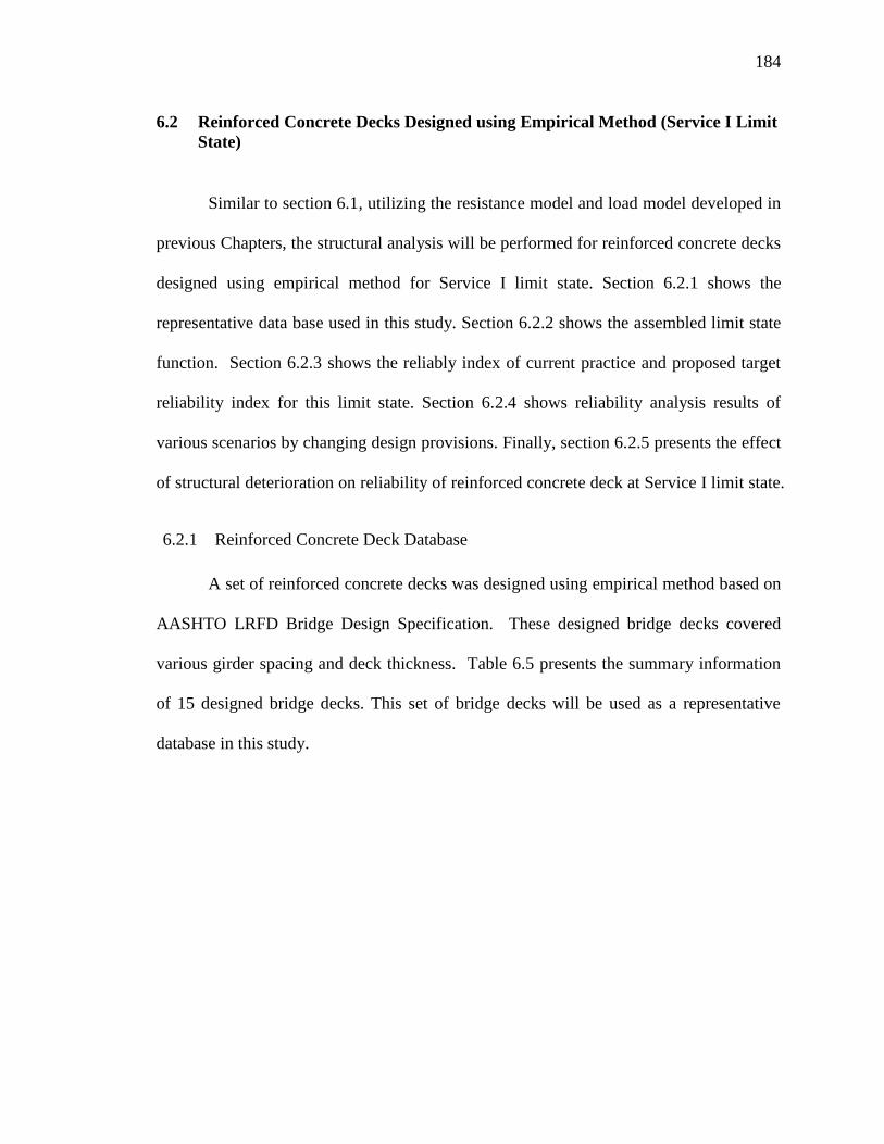
184
6.2 Reinforced Concrete Decks Designed using Empirical Method (Service I Limit
State)
Similar to section 6.1, utilizing the resistance model and load model developed in
previous Chapters, the structural analysis will be performed for reinforced concrete decks
designed using empirical method for Service I limit state. Section 6.2.1 shows the
representative data base used in this study. Section 6.2.2 shows the assembled limit state
function. Section 6.2.3 shows the reliably index of current practice and proposed target
reliability index for this limit state. Section 6.2.4 shows reliability analysis results of
various scenarios by changing design provisions. Finally, section 6.2.5 presents the effect
of structural deterioration on reliability of reinforced concrete deck at Service I limit state.
6.2.1 Reinforced Concrete Deck Database
A set of reinforced concrete decks was designed using empirical method based on
AASHTO LRFD Bridge Design Specification. These designed bridge decks covered
various girder spacing and deck thickness. Table 6.5 presents the summary information
of 15 designed bridge decks. This set of bridge decks will be used as a representative
database in this study.

185
Table 6.5 Information of 15 Bridge Decks that Designed using AASHTO Empirical Deck
Design Method
Deck Group# Girder Spacing (ft.) Deck Thickness (in.)
1 6
7
7.5
8
2 8
7.5
8
8.5
3 10
8
8.5
9
9.5
4 12
8
8.5
9
9.5
10
6.2.2 Limit State Function for Reinforced Concrete Decks Designed using Empirical
Method
The limit state function for reinforced concrete decks designed using Empirical
Method is the same as the one for concrete deck designed using traditional method except
that the resistance is different since arching action is considered for concrete decks
designed using empirical method. Based on the resistance and load model developed
from previous Chapters, the limit state function for reinforced concrete deck designed
using empirical method can be expressed as:

186
2 2' 2
1max
2
2
3 3 2 0.85
(4 9 ) 42
2
s s c s s s s cc s r c
s s c s
c
A E E bd A E A E E bdw E M f dG M
d A E E bd Asd
Eq. 6.8
6.2.3 Target Reliability Index for Service I Limit State (Empirical Deck)
Regardless of the design method that has been used during the design of
reinforced concrete deck, the targeted reliability level should be the same for same
exposure condition. For instance, when a concrete deck was designed in New Jersey, the
same reliability level is expected regardless of design method. Thus, the target reliability
indices proposed in section 6.1.3 are used also for the reliability analysis of concrete deck
designed using empirical design method.
6.2.4 Reliability analysis results for Service I Limit State
6.2.4.1 Class 1 Exposure Condition (Maximum Crack Width of 0.017 in)
Figure 6.20 and Figure 6.21 present the reliability indices for various bridge decks
designed using a live load factor of 1.0 over one year period, which reflected the
reliability level of current design. It can be observed that the average reliability index is
around 1.24 and 0.13 for positive and negative moment regions, respectively.

187
Figure 6.20 Reliability Indices of Various Bridge Decks Designed Using 1.0 Live Load
Factor over 1 Year Returning Period (ADTT=1000), Positive Moment Region.
Figure 6.21 Reliability Indices of Various Bridge Decks Designed Using 1.0 Live Load
Factor over 1 Year Returning Period (ADTT=1000), Negative Moment Region.
Figure 6.22 and Figure 6.23 present the reliability indices for an ADTT of 2500. It
can be observed that the average reliability index is around 0.71 and -0.40 for positive
and negative moment regions, respectively.

188
Figure 6.22 Reliability Indices of Various Bridge Decks Designed Using 1.0 Live Load
Factor over 1 Year Returning Period (ADTT=2500), Positive Moment Region.
Figure 6.23 Reliability Indices of Various Bridge Decks Designed Using 1.0 Live Load
Factor over 1 Year Returning Period (ADTT=2500), Negative Moment Region.
Figure 6.24 and Figure 6.25 present the reliability indices for various bridge decks
designed using a live load factor of 1.0 over one year period for an ADTT of 5000. It can
be observed that the average reliability index is around 0.57 and -0.51 for positive and
negative moment region, respectively.
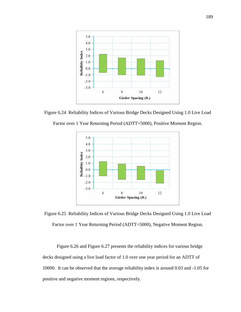
189
Figure 6.24 Reliability Indices of Various Bridge Decks Designed Using 1.0 Live Load
Factor over 1 Year Returning Period (ADTT=5000), Positive Moment Region.
Figure 6.25 Reliability Indices of Various Bridge Decks Designed Using 1.0 Live Load
Factor over 1 Year Returning Period (ADTT=5000), Negative Moment Region.
Figure 6.26 and Figure 6.27 presents the reliability indices for various bridge
decks designed using a live load factor of 1.0 over one year period for an ADTT of
10000. It can be observed that the average reliability index is around 0.03 and -1.05 for
positive and negative moment regions, respectively.
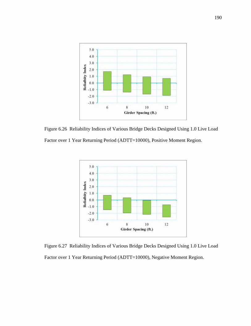
190
Figure 6.26 Reliability Indices of Various Bridge Decks Designed Using 1.0 Live Load
Factor over 1 Year Returning Period (ADTT=10000), Positive Moment Region.
Figure 6.27 Reliability Indices of Various Bridge Decks Designed Using 1.0 Live Load
Factor over 1 Year Returning Period (ADTT=10000), Negative Moment Region.
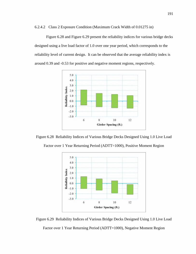
191
6.2.4.2 Class 2 Exposure Condition (Maximum Crack Width of 0.01275 in)
Figure 6.28 and Figure 6.29 present the reliability indices for various bridge decks
designed using a live load factor of 1.0 over one year period, which corresponds to the
reliability level of current design. It can be observed that the average reliability index is
around 0.39 and -0.53 for positive and negative moment regions, respectively.
Figure 6.28 Reliability Indices of Various Bridge Decks Designed Using 1.0 Live Load
Factor over 1 Year Returning Period (ADTT=1000), Positive Moment Region
Figure 6.29 Reliability Indices of Various Bridge Decks Designed Using 1.0 Live Load
Factor over 1 Year Returning Period (ADTT=1000), Negative Moment Region

192
Figure 6.30 and Figure 6.31 present the reliability indices for an ADTT of 2500. It
can be observed that the average reliability index is around -0.17 and -0.98 for positive
and negative moment region, respectively.
Figure 6.30 Reliability Indices of Various Bridge Decks Designed Using 1.0 Live Load
Factor over 1 Year Returning Period (ADTT=2500), Positive Moment Region.
Figure 6.31 Reliability Indices of Various Bridge Decks Designed Using 1.0 Live Load
Factor over 1 Year Returning Period (ADTT=2500), Negative Moment Region.
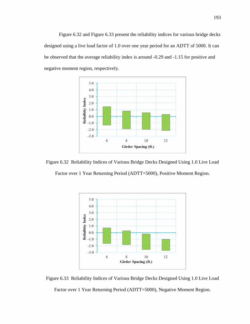
193
Figure 6.32 and Figure 6.33 present the reliability indices for various bridge decks
designed using a live load factor of 1.0 over one year period for an ADTT of 5000. It can
be observed that the average reliability index is around -0.29 and -1.15 for positive and
negative moment region, respectively.
Figure 6.32 Reliability Indices of Various Bridge Decks Designed Using 1.0 Live Load
Factor over 1 Year Returning Period (ADTT=5000), Positive Moment Region.
Figure 6.33 Reliability Indices of Various Bridge Decks Designed Using 1.0 Live Load
Factor over 1 Year Returning Period (ADTT=5000), Negative Moment Region.

194
Figure 6.34 and Figure 6.35 presents the reliability indices for various bridge
decks designed using a live load factor of 1.0 over one year period for an ADTT of
10000. It can be observed that the average reliability index is around -0.78 and -1.66 for
positive and negative moment region, respectively.
Figure 6.34 Reliability Indices of Various Bridge Decks Designed Using 1.0 Live Load
Factor over 1 Year Returning Period (ADTT=10000), Positive Moment Region.
Figure 6.35 Reliability Indices of Various Bridge Decks Designed Using 1.0 Live Load
Factor over 1 Year Returning Period (ADTT=10000), Negative Moment Region.
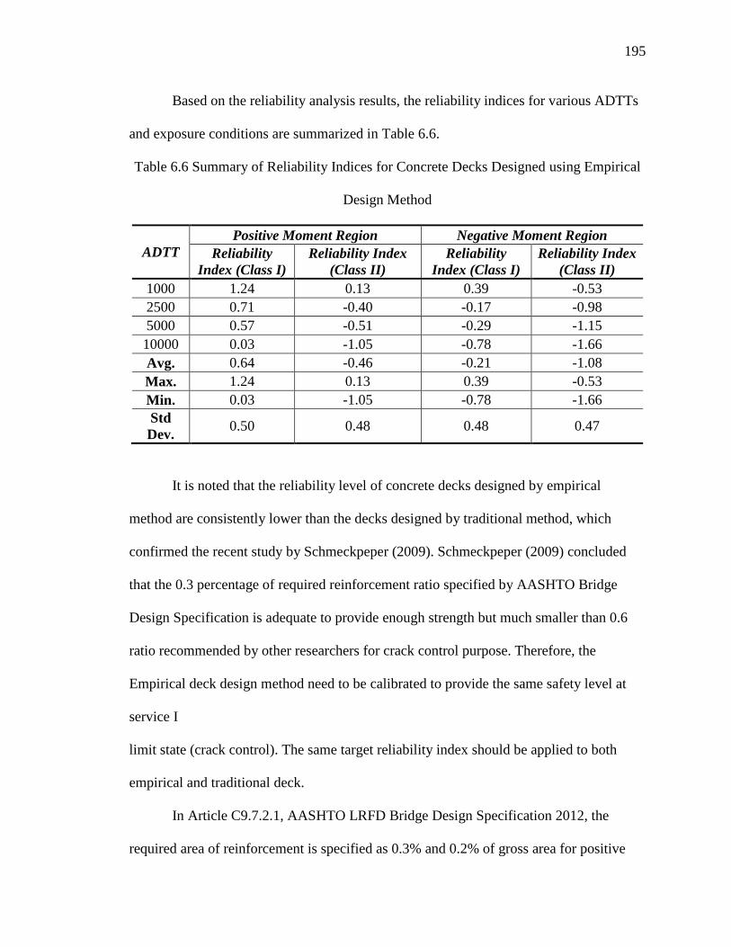
195
Based on the reliability analysis results, the reliability indices for various ADTTs
and exposure conditions are summarized in Table 6.6.
Table 6.6 Summary of Reliability Indices for Concrete Decks Designed using Empirical
Design Method
ADTT
Positive Moment Region Negative Moment Region
Reliability
Index (Class I)
Reliability Index
(Class II)
Reliability
Index (Class I)
Reliability Index
(Class II)
1000 1.24 0.13 0.39 -0.53
2500 0.71 -0.40 -0.17 -0.98
5000 0.57 -0.51 -0.29 -1.15
10000 0.03 -1.05 -0.78 -1.66
Avg. 0.64 -0.46 -0.21 -1.08
Max. 1.24 0.13 0.39 -0.53
Min. 0.03 -1.05 -0.78 -1.66
Std
Dev. 0.50 0.48 0.48 0.47
It is noted that the reliability level of concrete decks designed by empirical
method are consistently lower than the decks designed by traditional method, which
confirmed the recent study by Schmeckpeper (2009). Schmeckpeper (2009) concluded
that the 0.3 percentage of required reinforcement ratio specified by AASHTO Bridge
Design Specification is adequate to provide enough strength but much smaller than 0.6
ratio recommended by other researchers for crack control purpose. Therefore, the
Empirical deck design method need to be calibrated to provide the same safety level at
service I
limit state (crack control). The same target reliability index should be applied to both
empirical and traditional deck.
In Article C9.7.2.1, AASHTO LRFD Bridge Design Specification 2012, the
required area of reinforcement is specified as 0.3% and 0.2% of gross area for positive
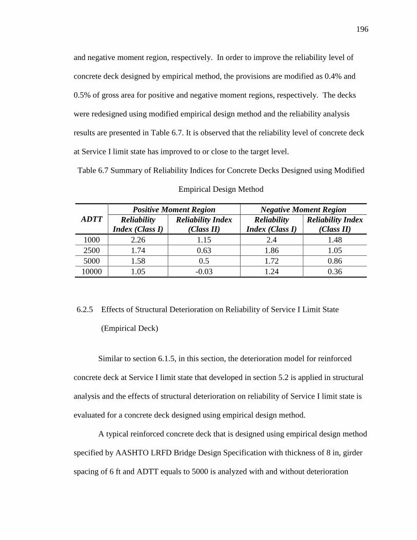
196
and negative moment region, respectively. In order to improve the reliability level of
concrete deck designed by empirical method, the provisions are modified as 0.4% and
0.5% of gross area for positive and negative moment regions, respectively. The decks
were redesigned using modified empirical design method and the reliability analysis
results are presented in Table 6.7. It is observed that the reliability level of concrete deck
at Service I limit state has improved to or close to the target level.
Table 6.7 Summary of Reliability Indices for Concrete Decks Designed using Modified
Empirical Design Method
ADTT
Positive Moment Region Negative Moment Region
Reliability
Index (Class I)
Reliability Index
(Class II)
Reliability
Index (Class I)
Reliability Index
(Class II)
1000 2.26 1.15 2.4 1.48
2500 1.74 0.63 1.86 1.05
5000 1.58 0.5 1.72 0.86
10000 1.05 -0.03 1.24 0.36
6.2.5 Effects of Structural Deterioration on Reliability of Service I Limit State
(Empirical Deck)
Similar to section 6.1.5, in this section, the deterioration model for reinforced
concrete deck at Service I limit state that developed in section 5.2 is applied in structural
analysis and the effects of structural deterioration on reliability of Service I limit state is
evaluated for a concrete deck designed using empirical design method.
A typical reinforced concrete deck that is designed using empirical design method
specified by AASHTO LRFD Bridge Design Specification with thickness of 8 in, girder
spacing of 6 ft and ADTT equals to 5000 is analyzed with and without deterioration
197
model applied. As shown in Figure 6.19, it is observed that the deterioration of structure
has significant effect on the reliability of structure, especially for long duration.
Figure 6.36 reliability index for reinforced concrete deck designed by empirical method
(with and w/o deterioration)
6.3 Prestressed Concrete Girders (Service III Limit State)
In this section, utilizing the resistance model and load model developed in
previous Chapters, the reliability analysis will be performed for prestressed concrete
girders at Service III limit state. Section 6.3.1 shows the representative data base used in
this study. Section 6.3.2 shows the assembled limit state. Section 6.3.3 shows the reliably
index of current practice and proposed target reliability index for this limit state. Section
6.3.4 shows reliability analysis results of various scenarios by changing design provisions.
Finally, section 6.3.5 presents the effect of structural deterioration on reliability of
prestressed concrete girder at Service III limit state.

198
6.3.1 Prestressed Concrete Girder Database
A database of existing prestressed concrete girder bridges was extracted from the
database of bridges used in the NCHRP 12-78 project (Mlynarski, et. al. 2011) which
were all taken from the NBI database. The database used in this study included 30 I- and
bulb-T girder bridges, 31 adjacent box girder bridges and 36 spread box girder bridges.
This database was used to evaluate the reliability level of existing prestressed concrete
bridges. Besides database for existing bridges, a huge bridge database was developed to
include major design parameters. These parameters include concrete strength, tensile
stress limit, girder type, span length, design vehicle type, live load factor for Service III
limit state. Figure 6.37 shows various parameters that varied to generate large amount of
bridges. Table 6.8 shows how many cases that have been considered for each parameter.
There are a total more than 400 bridges included in prestressed concrete girder database.
More detailed information of bridge database can be found in Appendix A.
Table 6.8 Summary of Matrix of Designed Parameters
Design Parameter Number of Cases Remarks
Concrete Strength 3 6 ksi, 8 ksi, 10 ksi
Girder Type 4 AASHTO I, Spread Box,
Adjacent Box, ASBI Box
Tensile Stress Limit 4 √ , √ ,
√ , √ ,
Live Load Factor 2 0.8, 1.0
Span Length 10 30 ft~220 ft
Design Vehicle 2 NJDOT Permit Vehicle, HL-93

199
Figure 6.37 Composition of Simulated Bridge Database
6.3.2 Limit State Function for Service III Limit State
The limit state function of Service III limit state is expressed in terms of mid-span
moment. It is formulated for three performance levels, decompression, maximum tensile
stress limit, maximum crack width limit, as shown below:
Decompression Level: Dec QG M M Eq. 6.9
Maximum Tensile Stress Limit Level: T QG M M Eq. 6.10
Maximum Crack Width Limit Level: Cr QG M M Eq. 6.11
As shown in Chapter 3, the resistance moment can be expressed in a uniform
formula as:
Simulated Bridge
Database
Concrete Strength
Tensile Stress Limit
Live Load Factor
Design Vehicle Model
Span Length
Girder Type
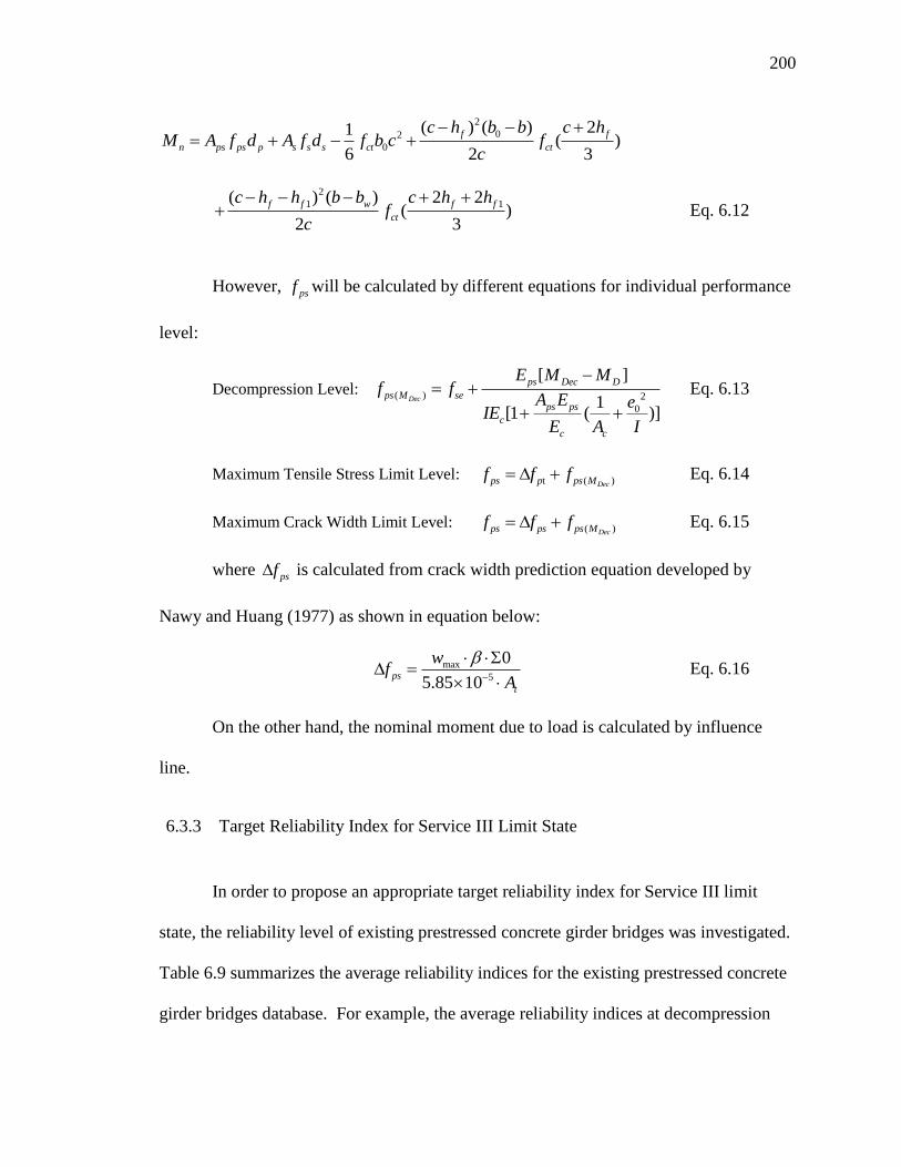
200
2
02
0
( ) ( ) 21( )
6 2 3
f f
n ps ps p s s s ct ct
c h b b c hM A f d A f d f b c f
c
2
1 1( ) ( ) 2 2( )
2 3
f f w f f
ct
c h h b b c h hf
c
Eq. 6.12
However, psf will be calculated by different equations for individual performance
level:
Decompression Level: ( ) 2
0
[ ]
1[1 ( )]
Dec
ps Dec D
ps M seps ps
c
c c
E M Mf f
A E eIE
E A I
Eq. 6.13
Maximum Tensile Stress Limit Level: t ( )Decps p ps Mf f f Eq. 6.14
Maximum Crack Width Limit Level: ( )Decps ps ps Mf f f Eq. 6.15
where psf is calculated from crack width prediction equation developed by
Nawy and Huang (1977) as shown in equation below:
max
5
0
5.85 10ps
t
wf
A
Eq. 6.16
On the other hand, the nominal moment due to load is calculated by influence
line.
6.3.3 Target Reliability Index for Service III Limit State
In order to propose an appropriate target reliability index for Service III limit
state, the reliability level of existing prestressed concrete girder bridges was investigated.
Table 6.9 summarizes the average reliability indices for the existing prestressed concrete
girder bridges database. For example, the average reliability indices at decompression

201
level, maximum allowable tensile stress limit under service loads of 0.19t cf f , and
maximum allowable crack width limit of 0.016 are 0.74, 1.05, and 2.69, respectively, for
an ADTT of 5000 and a return period of one year.
Table 6.9 Summary of Reliability Indices for Existing Bridges with One Lane Loaded
and Return Period of 1 Year
Performance Levels
ADTT
ADTT
=1000
ADTT
=2500
ADTT
=5000
ADTT
=10000
Decompression 0.95 0.85 0.74 0.61
Maximum
Tensile
Stress
Limit
0.0948t cf f
1.15 1.01 0.94 0.82
0.19t cf f
1.24 1.14 1.05 0.95
0.25t cf f
1.40 1.27 1.19 1.07
Maximum
Crack
Width
0.008 in 2.29 2.21 1.99 1.85
0.012 in 2.65 2.60 2.37 2.22
0.016 in 3.06 2.89 2.69 2.56
A database of simulated simple span bridges was designed using AASHTO I-
girder sections for four different cases. The simulated bridges have span of 30, 60, 80,
100 and 140 ft and girder spacing of 6, 8, 10 and 12 ft. This database was analyzed to
determine the effect of the change in the method of estimating prestressing losses (pre-
2004 and current methods) and the design environment (“severe corrosive conditions”
and “normal” or “not worse than moderate corrosion conditions”). The two
environmental conditions are signified by the maximum concrete tensile stress limit (
0.0948t cf f or 0.19t cf f ) used in the design. The four cases of design
considered were:

202
Case 1: AASHTO LRFD with maximum concrete tensile stress of 0.0948t cf f and
pre-2005 prestress loss method
Case 2: AASHTO LRFD with maximum concrete tensile stress of 0.0948t cf f and
current (2012) prestress loss method
Case 3: AASHTO LRFD with maximum concrete tensile stress of 0.19t cf f and pre-
2005 prestress loss method
Case 4: AASHTO LRFD with maximum concrete tensile stress of 0.19t cf f and
current (2012) prestress loss method
Table 6.10 and Table 6.11 show the span length and girder spacing along with the
calculated reliability indices for I-girder bridges designed for maximum concrete tensile
stress 0.0948t cf f (Case 1 and Case 2) and 0.19t cf f (Case 3 and Case 4),
respectively, for ADTT 5000.
In performing the design, the cases using current prestress loss method (Case 2
and Case 4) were designed using the smallest possible AASHTO girder size. To
facilitate the comparisons, Case 1 and Case 3 were then designed using the same
AASHTO section used for the same span and girder spacing for Case 2 and 4,
respectively. In some cases, the section used for Case 2 or Case 4 was too small to be
used for the corresponding Case 1 or Case 3. In such cases no design is shown in Table
6.10 and Table 6.11. For the 140 ft span bridges with 12 ft girder spacing, no AASHTO
I-girder section was sufficient.
203
Bridges designed for Case 1 and Case 3 are also thought to be similar to those
designed using AASHTO Standard specifications for the two environmental conditions.
The reliability indices calculated for Case 1 and Case 3 represent the inherent reliability
of bridges currently on the system as most of them were designed before 2005. Case 2
and Case 4 generally represent the inherent reliability of newer bridges designed using
the 2005 and later versions of AASHTO LRFD for severe and normal environmental
conditions, respectively.
Comparing Case 1 to Case 2 and Case 3 to Case 4 shows the effect of changing
the prestressing loss method.
Using the current prestress loss method resulted in smaller number of strands than
the old loss method. As shown in Table 6.10 and Table 6.11, the lower number of
strands resulted in lower reliability index for bridges designed using the new (current)
prestress loss method.
As shown in Table 6.10 and Table 6.11, regardless of the loss method and/or the
limit state used, the reliability indices for each case varied significantly. This suggested
the need to calibrate the limit state to develop a combination of load and resistance
factors that produce a more uniform reliability index across different spans and girder
spacings.
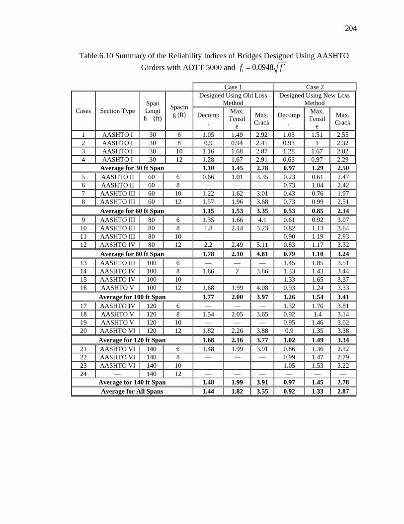
204
Table 6.10 Summary of the Reliability Indices of Bridges Designed Using AASHTO
Girders with ADTT 5000 and 0.0948t cf f
Case 1 Case 2
Cases Section Type
Span
Lengt
h (ft)
Spacin
g (ft)
Designed Using Old Loss
Method
Designed Using New Loss
Method
Decomp
.
Max.
Tensil
e
Max.
Crack
Decomp
.
Max.
Tensil
e
Max.
Crack
1 AASHTO I 30 6 1.05 1.49 2.92 1.03 1.51 2.55
2 AASHTO I 30 8 0.9 0.94 2.41 0.93 1 2.32
3 AASHTO I 30 10 1.16 1.68 2.87 1.28 1.67 2.82
4 AASHTO I 30 12 1.28 1.67 2.91 0.63 0.97 2.29
Average for 30 ft Span 1.10 1.45 2.78 0.97 1.29 2.50
5 AASHTO II 60 6 0.66 1.01 3.35 0.23 0.61 2.47
6 AASHTO II 60 8 — — — 0.73 1.04 2.42
7 AASHTO III 60 10 1.22 1.62 3.01 0.43 0.76 1.97
8 AASHTO III 60 12 1.57 1.96 3.68 0.73 0.99 2.51
Average for 60 ft Span 1.15 1.53 3.35 0.53 0.85 2.34
9 AASHTO III 80 6 1.35 1.66 4.1 0.61 0.92 3.07
10 AASHTO III 80 8 1.8 2.14 5.23 0.82 1.13 3.64
11 AASHTO III 80 10 — — — 0.90 1.19 2.93
12 AASHTO IV 80 12 2.2 2.49 5.11 0.83 1.17 3.32
Average for 80 ft Span 1.78 2.10 4.81 0.79 1.10 3.24
13 AASHTO III 100 6 — — — 1.45 1.85 3.51
14 AASHTO IV 100 8 1.86 2 3.86 1.33 1.43 3.44
15 AASHTO IV 100 10 — — — 1.33 1.65 3.37
16 AASHTO V 100 12 1.68 1.99 4.08 0.93 1.24 3.33
Average for 100 ft Span 1.77 2.00 3.97 1.26 1.54 3.41
17 AASHTO IV 120 6 — — — 1.32 1.76 3.81
18 AASHTO V 120 8 1.54 2.05 3.65 0.92 1.4 3.14
19 AASHTO V 120 10 — — — 0.95 1.46 3.02
20 AASHTO VI 120 12 1.82 2.26 3.88 0.9 1.35 3.38
Average for 120 ft Span 1.68 2.16 3.77 1.02 1.49 3.34
21 AASHTO VI 140 6 1.48 1.99 3.91 0.86 1.36 2.32
22 AASHTO VI 140 8 — — — 0.99 1.47 2.79
23 AASHTO VI 140 10 — — — 1.05 1.53 3.22
24 — 140 12 — — — — — —
Average for 140 ft Span 1.48 1.99 3.91 0.97 1.45 2.78
Average for All Spans 1.44 1.82 3.55 0.92 1.33 2.87

205
Table 6.11 Summary of the Reliability Indices of Bridges Designed Using AASHTO
Girders with ADTT 5000 and 0.19t cf f
Case 3 Case 4
Cases Section Type
Span
Length
(ft)
Spacing
(ft)
Designed Using Old Loss
Method
Designed Using New Loss
Method
Decomp. Max.
Tensile
Max.
Crack Decomp.
Max.
Tensile
Max.
Crack
1 AASHTO I 30 6 1 1.55 2.39 0.97 1.55 2.46
2 AASHTO I 30 8 0.94 0.92 2.35 0.91 1.00 2.16
3 AASHTO I 30 10 1.29 1.66 2.91 1.18 1.66 2.79
4 AASHTO I 30 12 1.3 1.72 3.02 1.26 1.70 2.91
Average for 30 ft Span 1.13 1.46 2.67 1.08 1.48 2.58
5 AASHTO II 60 6 0.74 1.13 3.11 0.18 0.58 2.41
6 AASHTO II 60 8 1.04 1.39 2.82 0.28 0.66 1.91
7 AASHTO III 60 10 0.42 0.79 2.05 0.42 0.78 2.07
8 AASHTO III 60 12 0.66 1.00 2.5 0.68 0.96 2.53
Average for 60 ft Span 0.72 1.08 2.62 0.39 0.75 2.23
9 AASHTO III 80 6 0.56 0.97 3.13 0.13 0.51 2.53
10 AASHTO III 80 8 1.06 1.46 3.43 0.42 0.78 3.2
11 AASHTO III 80 10 1.58 1.84 3.65 0.37 0.65 2.72
12 AASHTO IV 80 12 0.83 1.15 3.72 0.51 0.87 3.11
Average for 80 ft Span 1.01 1.36 3.48 0.36 0.70 2.89
13 AASHTO III 100 6 — — — 0.82 1.23 3.44
14 AASHTO IV 100 8 1.31 1.42 3.6 0.69 0.76 2.76
15 AASHTO IV 100 10 1.8 1.98 3.67 0.75 1.04 3.12
16 AASHTO V 100 12 1.08 1.37 3.43 0.4 0.72 2.55
Average for 100 ft Span 1.40 1.59 3.57 0.67 0.94 2.97
17 AASHTO IV 120 6 1.53 1.98 3.71 0.7 1.28 3.1
18 AASHTO V 120 8 0.9 1.30 3.31 0.46 0.85 2.55
19 AASHTO V 120 10 1.25 1.65 3.35 0.26 0.78 2.68
20 AASHTO VI 120 12 1.19 1.66 3.37 0.47 0.91 2.69
Average for 120 ft Span 1.22 1.65 3.44 0.47 0.96 2.76
21 AASHTO VI 140 6 0.84 1.41 3.23 0.28 0.82 2.41
22 AASHTO VI 140 8 1.22 1.68 3.3 0.53 0.98 3.04
23 AASHTO VI 140 10 — — — 0.62 1.08 2.46
24 — 140 12 — — — — — —
Average for 140 ft Span 1.03 1.55 3.27 0.48 0.96 2.64
Average for All Spans 1.07 1.43 3.15 0.58 0.96 2.68
206
The target reliability indices were selected based on the calculated average values
of the reliability levels of existing bridges and previous practices with some consideration
given to experiences from other Codes (Eurocode and ISO 2394 Document). As
indicated earlier, a return period of 1 year was selected and an ADTT equal to 5000 was
used.
Table 6.12 shows the target reliability indices selected in this study. Notice that
the environmental condition for existing bridges was not known and that the two columns
showing the reliability indices of the simulated bridges is for cases where the old
prestressing loss method was used as these are thought to better represent the bridges
currently on the system.
For example, the reliability index of existing bridges, simulated bridges designed
for severe environments, and simulated bridges designed for normal environments, at the
decompression performance level is around 0.74, 1.44 and 1.07, respectively (See Table
6.9 through Table 6.12). Therefore, a target reliability index of 1.2 and 1.0 was selected
for the decompression performance level for bridges designed for severe environments
and bridges designed for normal environments, respectively. The reliability index of 1.0
means that 15 out of 100 bridges will probably have the bottom of the girder decompress
in any given year.
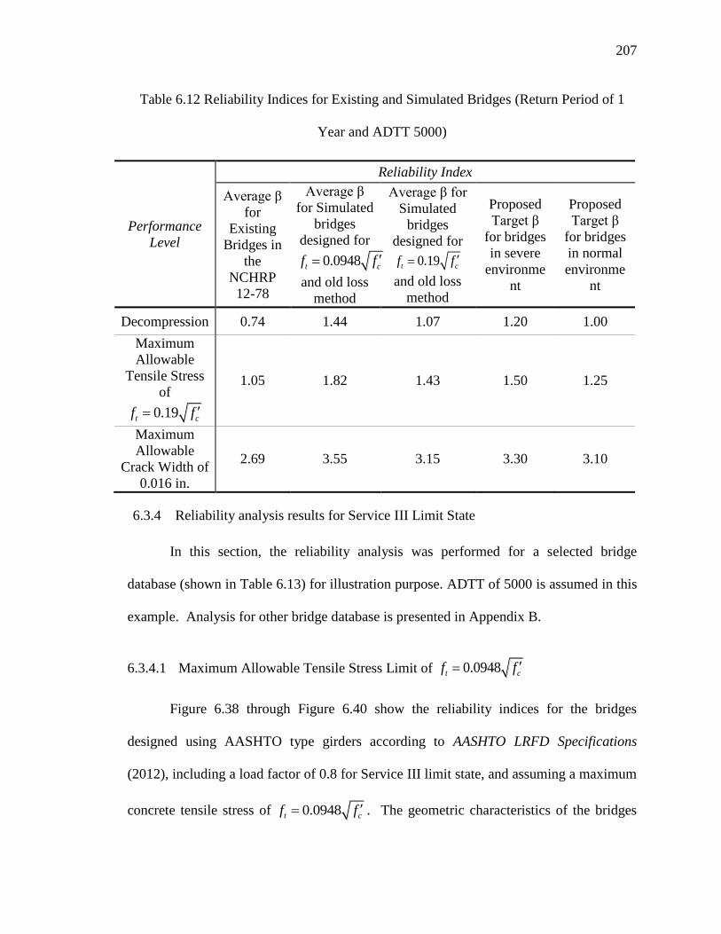
207
Table 6.12 Reliability Indices for Existing and Simulated Bridges (Return Period of 1
Year and ADTT 5000)
6.3.4 Reliability analysis results for Service III Limit State
In this section, the reliability analysis was performed for a selected bridge
database (shown in Table 6.13) for illustration purpose. ADTT of 5000 is assumed in this
example. Analysis for other bridge database is presented in Appendix B.
6.3.4.1 Maximum Allowable Tensile Stress Limit of 0.0948t cf f
Figure 6.38 through Figure 6.40 show the reliability indices for the bridges
designed using AASHTO type girders according to AASHTO LRFD Specifications
(2012), including a load factor of 0.8 for Service III limit state, and assuming a maximum
concrete tensile stress of 0.0948t cf f . The geometric characteristics of the bridges
Performance
Level
Reliability Index
Average β
for
Existing
Bridges in
the
NCHRP
12-78
Average β
for Simulated
bridges
designed for
0.0948t cf f
and old loss
method
Average β for
Simulated
bridges
designed for
0.19t cf f
and old loss
method
Proposed
Target β
for bridges
in severe
environme
nt
Proposed
Target β
for bridges
in normal
environme
nt
Decompression 0.74 1.44 1.07 1.20 1.00
Maximum
Allowable
Tensile Stress
of
0.19t cf f
1.05 1.82 1.43 1.50 1.25
Maximum
Allowable
Crack Width of
0.016 in.
2.69 3.55 3.15 3.30 3.10
208
are shown in Table 6.13. It was observed that the average reliability index for the
decompression limit state, maximum allowable tensile stress limit state, and maximum
allowable crack width limit state is 0.97, 1.31, and 3.06, respectively. Since the reliability
indices are lower than the target reliability indices and that the reliability indices are not
uniform across different spans, modifications to the load factor will be conducted in an
attempt to achieve higher, and more uniform, reliability indices.
As a second step, the bridges have been redesigned using a live load factor of 1.0
and the dead load and resistance factors were kept the same during the re-design. Table
6.14 shows the design geometric characteristics of the redesigned bridges.
Figure 6.41 through Figure 6.43 show the reliability indices for the re-designed
bridges using a live load factor of 1.0. The average reliability index for the
decompression limit state, the maximum allowable tensile stress limit state and the
maximum allowable crack width limit state is 1.33, 1.70, and 3.32, respectively. It was
observed that the reliability level of bridges became more uniform than for the case of
using a live load factor of 0.8, particularly for the decompression and maximum tensile
stress limit states. Therefore, a live load factor of 1.0 was proposed to be used if the
tensile stress is limited to 0.0948t cf f .
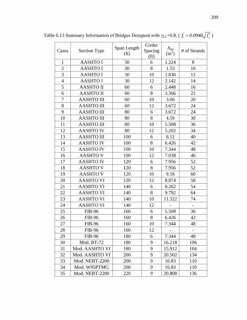
209
Table 6.13 Summary Information of Bridges Designed with γLL=0.8, ( 0.0948t cf f )
Cases Section Type Span Length
(ft)
Girder
Spacing
(ft)
Aps
(in2)
# of Strands
1 AASHTO I 30 6 1.224 8
2 AASHTO I 30 8 1.53 10
3 AASHTO I 30 10 1.836 12
4 AASHTO I 30 12 2.142 14
5 AASHTO II 60 6 2.448 16
6 AASHTO II 60 8 3.366 22
7 AASHTO III 60 10 3.06 20
8 AASHTO III 60 12 3.672 24
9 AASHTO III 80 6 3.672 24
10 AASHTO III 80 8 4.59 30
11 AASHTO III 80 10 5.508 36
12 AASHTO IV 80 12 5.202 34
13 AASHTO III 100 6 6.12 40
14 AASHTO IV 100 8 6.426 42
15 AASHTO IV 100 10 7.344 48
16 AASHTO V 100 12 7.038 46
17 AASHTO IV 120 6 7.956 52
18 AASHTO V 120 8 7.956 52
19 AASHTO V 120 10 9.18 60
20 AASHTO VI 120 12 8.874 58
21 AASHTO VI 140 6 8.262 54
22 AASHTO VI 140 8 9.792 64
23 AASHTO VI 140 10 11.322 74
24 AASHTO VI 140 12 - -
25 FIB-96 160 6 5.508 36
26 FIB-96 160 8 6.426 42
27 FIB-96 160 10 7.344 48
28 FIB-96 160 12 - -
29 FIB-96 180 6 7.344 48
30 Mod. BT-72 180 9 16.218 106
31 Mod. AASHTO VI 180 9 15.912 104
32 Mod. AASHTO VI 200 9 20.502 134
33 Mod. NEBT-2200 200 9 16.83 110
34 Mod. W95PTMG 200 9 16.83 110
35 Mod. NEBT-2200 220 9 20.808 136

210
Figure 6.38 Reliability indices for bridges at decompression limit state (ADTT=5000),
γLL=0.8, ( 0.0948t cf f ).
Figure 6.39 Reliability indices for bridges at maximum allowable tensile stress limit state
(ADTT=5000), γLL=0.8, ( 0.0948t cf f ).

211
Figure 6.40 Reliability Indices for bridges at maximum allowable crack width limit state
(ADTT=5000), γLL=0.8, ( 0.0948t cf f ).
Figure 6.41 Reliability indices for bridges at decompression limit state (ADTT=5000),
γLL=1.0 ( 0.0948t cf f ).
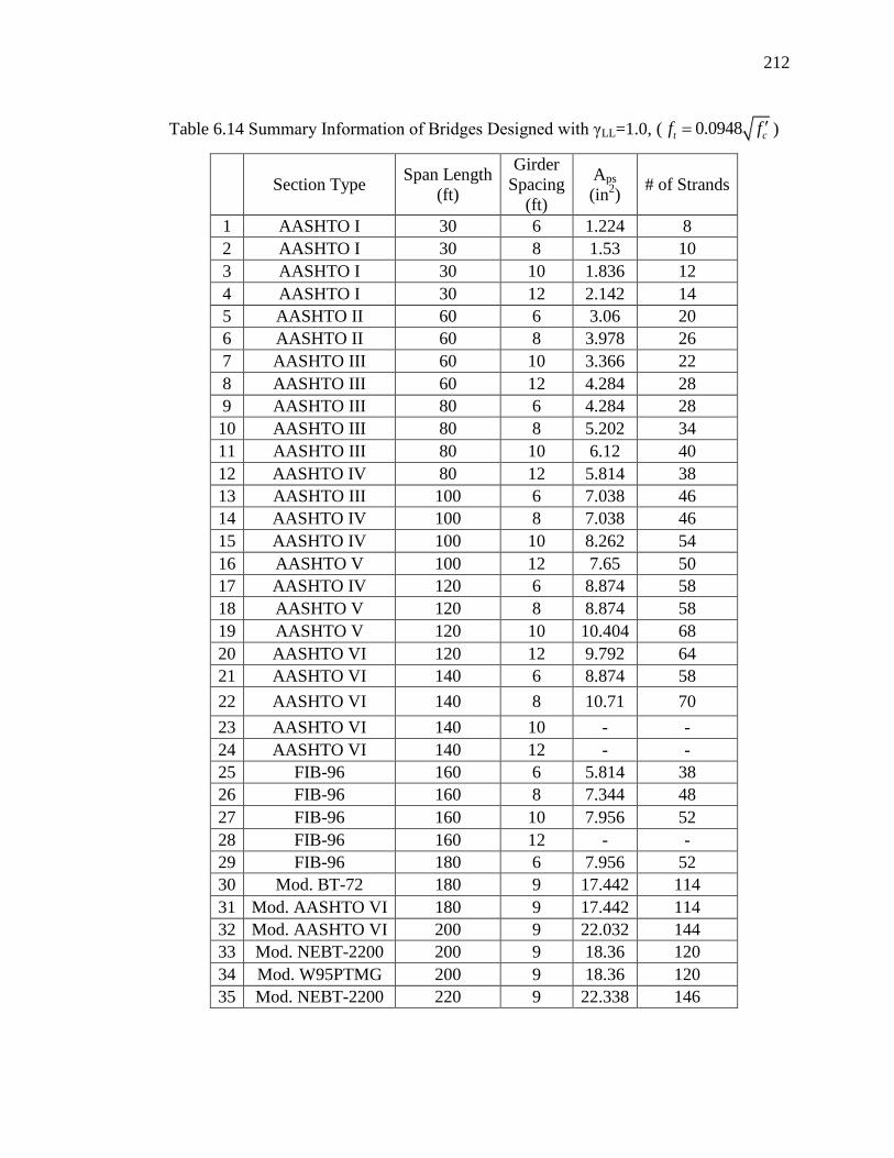
212
Table 6.14 Summary Information of Bridges Designed with γLL=1.0, ( 0.0948t cf f )
Section Type
Span Length
(ft)
Girder
Spacing
(ft)
Aps
(in2)
# of Strands
1 AASHTO I 30 6 1.224 8
2 AASHTO I 30 8 1.53 10
3 AASHTO I 30 10 1.836 12
4 AASHTO I 30 12 2.142 14
5 AASHTO II 60 6 3.06 20
6 AASHTO II 60 8 3.978 26
7 AASHTO III 60 10 3.366 22
8 AASHTO III 60 12 4.284 28
9 AASHTO III 80 6 4.284 28
10 AASHTO III 80 8 5.202 34
11 AASHTO III 80 10 6.12 40
12 AASHTO IV 80 12 5.814 38
13 AASHTO III 100 6 7.038 46
14 AASHTO IV 100 8 7.038 46
15 AASHTO IV 100 10 8.262 54
16 AASHTO V 100 12 7.65 50
17 AASHTO IV 120 6 8.874 58
18 AASHTO V 120 8 8.874 58
19 AASHTO V 120 10 10.404 68
20 AASHTO VI 120 12 9.792 64
21 AASHTO VI 140 6 8.874 58
22 AASHTO VI 140 8 10.71 70
23 AASHTO VI 140 10 - -
24 AASHTO VI 140 12 - -
25 FIB-96 160 6 5.814 38
26 FIB-96 160 8 7.344 48
27 FIB-96 160 10 7.956 52
28 FIB-96 160 12 - -
29 FIB-96 180 6 7.956 52
30 Mod. BT-72 180 9 17.442 114
31 Mod. AASHTO VI 180 9 17.442 114
32 Mod. AASHTO VI 200 9 22.032 144
33 Mod. NEBT-2200 200 9 18.36 120
34 Mod. W95PTMG 200 9 18.36 120
35 Mod. NEBT-2200 220 9 22.338 146

213
Figure 6.42 Reliability indices for bridges at maximum allowable tensile stress limit state
(ADTT=5000), γLL=1.0 ( 0.0948t cf f ).
Figure 6.43 Reliability indices for bridges at maximum allowable crack width limit state
(ADTT=1000), γLL=1.0 ( 0.0948t cf f ).
6.3.4.2 Maximum Allowable Tensile Stress Limit of 0.19t cf f
In this section, the work described under section 6.3.4.1 above was repeated
except that the girders were redesigned assuming maximum concrete tensile stress of
0.19t cf f . The detailed information of design can be found in Appendix A.

214
Figure 6.44 through Figure 6.46 show the reliability indices for the bridges
designed using AASHTO type girders according to AASHTO LRFD Specifications
(2012), including a load factor of 0.8 for Service III limit state, and assuming a maximum
concrete tensile stress of 0.19t cf f . It was observed that the average reliability index
for the decompression limit state, maximum allowable tensile stress limit state, and
maximum allowable crack width limit state is 0.68, 1.1, and 2.82, respectively. As a
second step, the bridges have been redesigned using a live load factor of 1.0 and the dead
load and resistance factors were kept the same during the re-design.
Figure 6.47 through Figure 6.49 show the reliability indices for the re-designed
bridges using a live load factor of 1.0. The average reliability index for the
decompression limit state, the maximum allowable tensile stress limit state and the
maximum allowable crack width limit state is 1.00, 1.41, and 3.14, respectively. It was
observed that the reliability level of bridges became more uniform than for the case of
using a live load factor of 0.8, particularly for the decompression and maximum tensile
stress limit states. Therefore, a live load factor of 1.0 was proposed to be used if the
tensile stress is limited to 0.19t cf f .

215
Figure 6.44 Reliability indices for bridges at decompression limit state (ADTT=5000),
γLL=0.8 ( 0.19t cf f ).
Figure 6.45 Reliability indices for bridges at maximum allowable tensile stress limit state
(ADTT=5000), γLL=0.8 ( 0.19t cf f ).
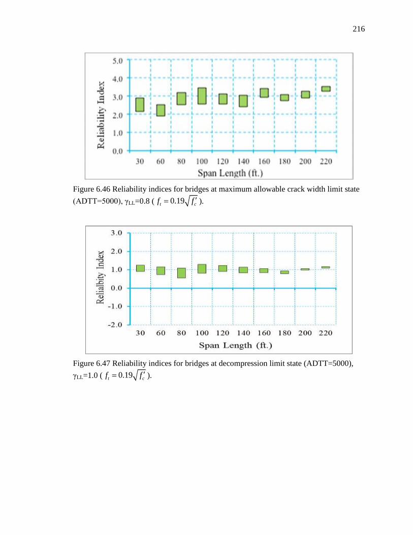
216
Figure 6.46 Reliability indices for bridges at maximum allowable crack width limit state
(ADTT=5000), γLL=0.8 ( 0.19t cf f ).
Figure 6.47 Reliability indices for bridges at decompression limit state (ADTT=5000),
γLL=1.0 ( 0.19t cf f ).

217
Figure 6.48 Reliability indices for bridges at maximum tensile stress limit state
(ADTT=5000), γLL=1.0 ( 0.19t cf f ).
Figure 6.49 Reliability indices for bridges at maximum crack width limit state
(ADTT=5000), γLL=1.0 ( 0.19t cf f ).
6.3.4.3 Maximum Allowable Tensile Stress Limit of 0.253t cf f
In this section, the work described under section 6.3.4.1 above was repeated
except that the girders were redesigned assuming maximum concrete tensile stress of
0.253t cf f . The detailed information of design can be found in Appendix A.

218
Figure 6.50 through Figure 6.52 show the reliability indices for the bridges
designed using AASHTO type girders according to AASHTO LRFD Specifications
(2012), including a load factor of 0.8 for Service III limit state, and assuming a maximum
concrete tensile stress of 0.253t cf f . It was observed that the average reliability
index for the decompression limit state, maximum allowable tensile stress limit state, and
maximum allowable crack width limit state is 0.06, 0.41, and 2.66, respectively. As a
second step, the bridges have been redesigned using a live load factor of 1.0 and the dead
load and resistance factors were kept the same during the re-design.
Figure 6.53 through Figure 6.55 show the reliability indices for the re-designed
bridges using a live load factor of 1.0. The average reliability index for the
decompression limit state, the maximum allowable tensile stress limit state and the
maximum allowable crack width limit state is 0.85, 1.23, and 2.92, respectively.
Figure 6.50 Reliability indices for bridges at decompression limit state (ADTT=5000),
γLL=0.8 ( 0.25t cf f ).

219
Figure 6.51 Reliability indices for bridges at maximum allowable tensile stress limit state
(ADTT=5000), γLL=0.8 ( 0.25t cf f ).
Figure 6.52 Reliability indices for bridges at maximum allowable crack width limit state
(ADTT=5000), γLL=0.8 ( 0.25t cf f ).
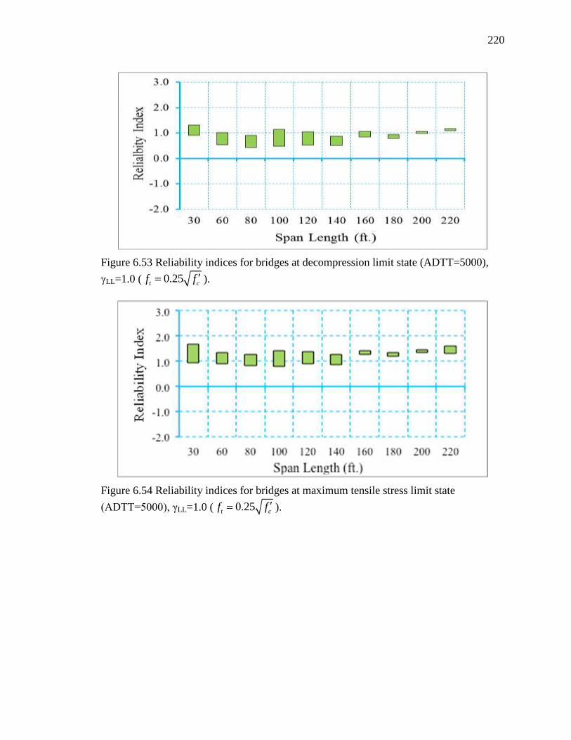
220
Figure 6.53 Reliability indices for bridges at decompression limit state (ADTT=5000),
γLL=1.0 ( 0.25t cf f ).
Figure 6.54 Reliability indices for bridges at maximum tensile stress limit state
(ADTT=5000), γLL=1.0 ( 0.25t cf f ).
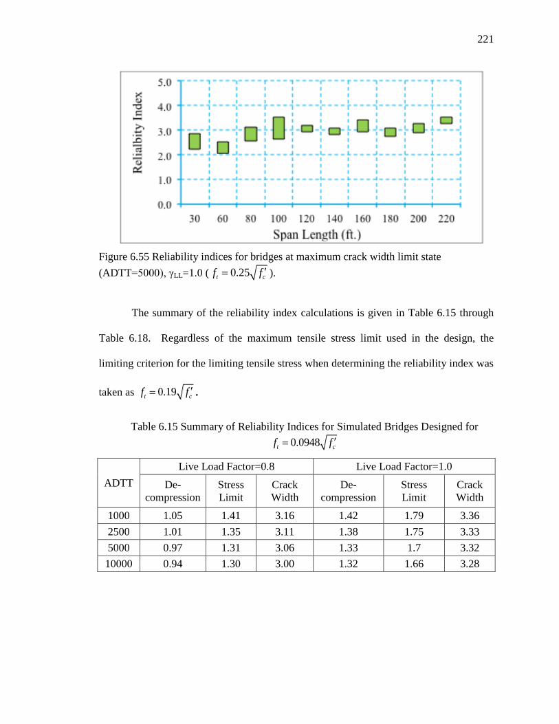
221
Figure 6.55 Reliability indices for bridges at maximum crack width limit state
(ADTT=5000), γLL=1.0 ( 0.25t cf f ).
The summary of the reliability index calculations is given in Table 6.15 through
Table 6.18. Regardless of the maximum tensile stress limit used in the design, the
limiting criterion for the limiting tensile stress when determining the reliability index was
taken as 0.19t cf f .
Table 6.15 Summary of Reliability Indices for Simulated Bridges Designed for
0.0948t cf f
ADTT
Live Load Factor=0.8 Live Load Factor=1.0
De-
compression
Stress
Limit
Crack
Width
De-
compression
Stress
Limit
Crack
Width
1000 1.05 1.41 3.16 1.42 1.79 3.36
2500 1.01 1.35 3.11 1.38 1.75 3.33
5000 0.97 1.31 3.06 1.33 1.7 3.32
10000 0.94 1.30 3.00 1.32 1.66 3.28

222
Table 6.16 Summary of Reliability Indices for Simulated Bridges Designed for
0.158t cf f
ADTT
Live Load Factor=0.8 Live Load Factor=1.0
De-
compression
Stress
Limit
Crack
Width
De-
compression
Stress
Limit
Crack
Width
1000 0.97 1.31 2.99 1.16 1.55 3.32
2500 0.83 1.19 2.96 1.12 1.50 3.29
5000 0.80 1.14 2.91 1.07 1.44 3.26
10000 0.76 1.11 2.85 1.04 1.40 3.22
Table 6.17 Summary of Reliability Indices for Simulated Bridges Designed for
0.19t cf f
ADTT
Live Load Factor=0.8 Live Load Factor=1.0
De-
compression
Stress
Limit
Crack
Width
De-
compression
Stress
Limit
Crack
Width
1000 0.84 1.27 2.92 1.11 1.53 3.25
2500 0.7 1.15 2.87 1.04 1.46 3.17
5000 0.68 1.1 2.82 1.00 1.41 3.14
10000 0.64 1.07 2.78 0.98 1.34 3.11
Table 6.18 Summary of Reliability Indices for Simulated Bridges Designed for
0.253t cf f
ADTT
Live Load Factor=0.8 Live Load Factor=1.0
De-
compression
Stress
Limit
Crack
Width
De-
compression
Stress
Limit
Crack
Width
1000 0.2 0.55 2.83 0.93 1.29 3.03
2500 0.08 0.49 2.77 0.89 1.27 2.95
5000 0.06 0.44 2.72 0.85 1.23 2.92
10000 0.02 0.41 2.66 0.82 1.2 2.88
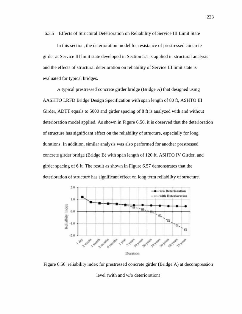
223
6.3.5 Effects of Structural Deterioration on Reliability of Service III Limit State
In this section, the deterioration model for resistance of prestressed concrete
girder at Service III limit state developed in Section 5.1 is applied in structural analysis
and the effects of structural deterioration on reliability of Service III limit state is
evaluated for typical bridges.
A typical prestressed concrete girder bridge (Bridge A) that designed using
AASHTO LRFD Bridge Design Specification with span length of 80 ft, ASHTO III
Girder, ADTT equals to 5000 and girder spacing of 8 ft is analyzed with and without
deterioration model applied. As shown in Figure 6.56, it is observed that the deterioration
of structure has significant effect on the reliability of structure, especially for long
durations. In addition, similar analysis was also performed for another prestressed
concrete girder bridge (Bridge B) with span length of 120 ft, ASHTO IV Girder, and
girder spacing of 6 ft. The result as shown in Figure 6.57 demonstrates that the
deterioration of structure has significant effect on long term reliability of structure.
Figure 6.56 reliability index for prestressed concrete girder (Bridge A) at decompression
level (with and w/o deterioration)
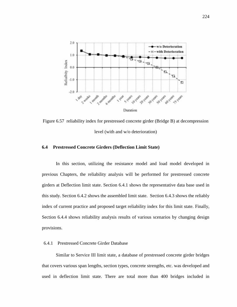
224
Figure 6.57 reliability index for prestressed concrete girder (Bridge B) at decompression
level (with and w/o deterioration)
6.4 Prestressed Concrete Girders (Deflection Limit State)
In this section, utilizing the resistance model and load model developed in
previous Chapters, the reliability analysis will be performed for prestressed concrete
girders at Deflection limit state. Section 6.4.1 shows the representative data base used in
this study. Section 6.4.2 shows the assembled limit state. Section 6.4.3 shows the reliably
index of current practice and proposed target reliability index for this limit state. Finally,
Section 6.4.4 shows reliability analysis results of various scenarios by changing design
provisions.
6.4.1 Prestressed Concrete Girder Database
Similar to Service III limit state, a database of prestressed concrete girder bridges
that covers various span lengths, section types, concrete strengths, etc. was developed and
used in deflection limit state. There are total more than 400 bridges included in

225
prestressed concrete girder database. More detailed information of bridge database can
be found in Appendix A.
6.4.2 Limit State Function for Deflection Limit State
The limit state function of Deflection limit state is expressed in terms of mid-span
moment as shown below:
R LLG M M Eq.
6.17
As shown in Chapter 3, for the uncracked section, the resistance moment can be
expressed in a uniform formula as:
.800
Cn
E ILM
C
Eq. 6.18
For the cracked section, the resistance moment canbe calculated using the
equation below:
. ( )[1 ]800
c e en cr D
g
E I ILM M M
C I
On the other hand, the nominal moment due to load is calculated by influence
line.
6.4.3 Target Reliability Index for Deflection Limit State
In order to propose an appropriate target reliability index for Deflection limit
state, the reliability level of existing prestressed concrete girder bridges was investigated.
Table 6.19 summarizes the average reliability indices for the existing prestressed concrete
girder bridges database. For example, the average reliability indices for uncracked
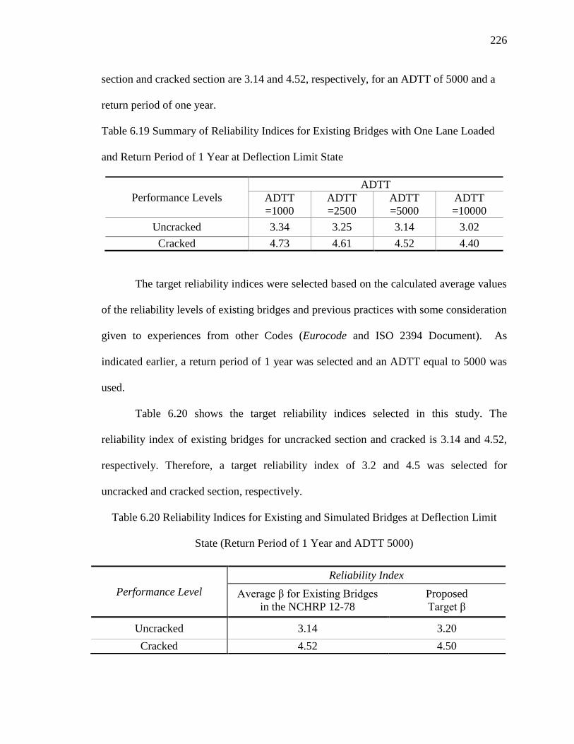
226
section and cracked section are 3.14 and 4.52, respectively, for an ADTT of 5000 and a
return period of one year.
Table 6.19 Summary of Reliability Indices for Existing Bridges with One Lane Loaded
and Return Period of 1 Year at Deflection Limit State
Performance Levels
ADTT
ADTT
=1000
ADTT
=2500
ADTT
=5000
ADTT
=10000
Uncracked 3.34 3.25 3.14 3.02
Cracked 4.73 4.61 4.52 4.40
The target reliability indices were selected based on the calculated average values
of the reliability levels of existing bridges and previous practices with some consideration
given to experiences from other Codes (Eurocode and ISO 2394 Document). As
indicated earlier, a return period of 1 year was selected and an ADTT equal to 5000 was
used.
Table 6.20 shows the target reliability indices selected in this study. The
reliability index of existing bridges for uncracked section and cracked is 3.14 and 4.52,
respectively. Therefore, a target reliability index of 3.2 and 4.5 was selected for
uncracked and cracked section, respectively.
Table 6.20 Reliability Indices for Existing and Simulated Bridges at Deflection Limit
State (Return Period of 1 Year and ADTT 5000)
Performance Level
Reliability Index
Average β for Existing Bridges
in the NCHRP 12-78
Proposed
Target β
Uncracked 3.14 3.20
Cracked 4.52 4.50
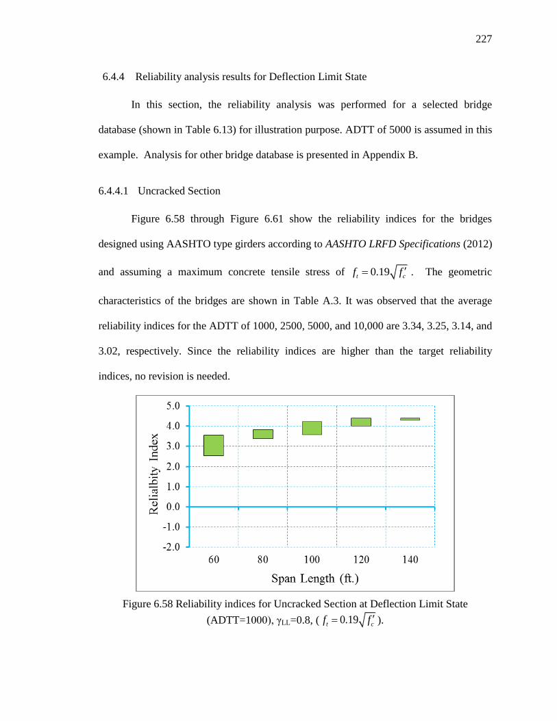
227
6.4.4 Reliability analysis results for Deflection Limit State
In this section, the reliability analysis was performed for a selected bridge
database (shown in Table 6.13) for illustration purpose. ADTT of 5000 is assumed in this
example. Analysis for other bridge database is presented in Appendix B.
6.4.4.1 Uncracked Section
Figure 6.58 through Figure 6.61 show the reliability indices for the bridges
designed using AASHTO type girders according to AASHTO LRFD Specifications (2012)
and assuming a maximum concrete tensile stress of 0.19t cf f . The geometric
characteristics of the bridges are shown in Table A.3. It was observed that the average
reliability indices for the ADTT of 1000, 2500, 5000, and 10,000 are 3.34, 3.25, 3.14, and
3.02, respectively. Since the reliability indices are higher than the target reliability
indices, no revision is needed.
Figure 6.58 Reliability indices for Uncracked Section at Deflection Limit State
(ADTT=1000), γLL=0.8, ( 0.19t cf f ).

228
Figure 6.59 Reliability indices for Uncracked Section at Deflection Limit State
(ADTT=2500), γLL=0.8, ( 0.19t cf f ).
Figure 6.60 Reliability Indices for Uncracked Section at Deflection Limit State
(ADTT=5000), γLL=0.8, ( 0.19t cf f ).
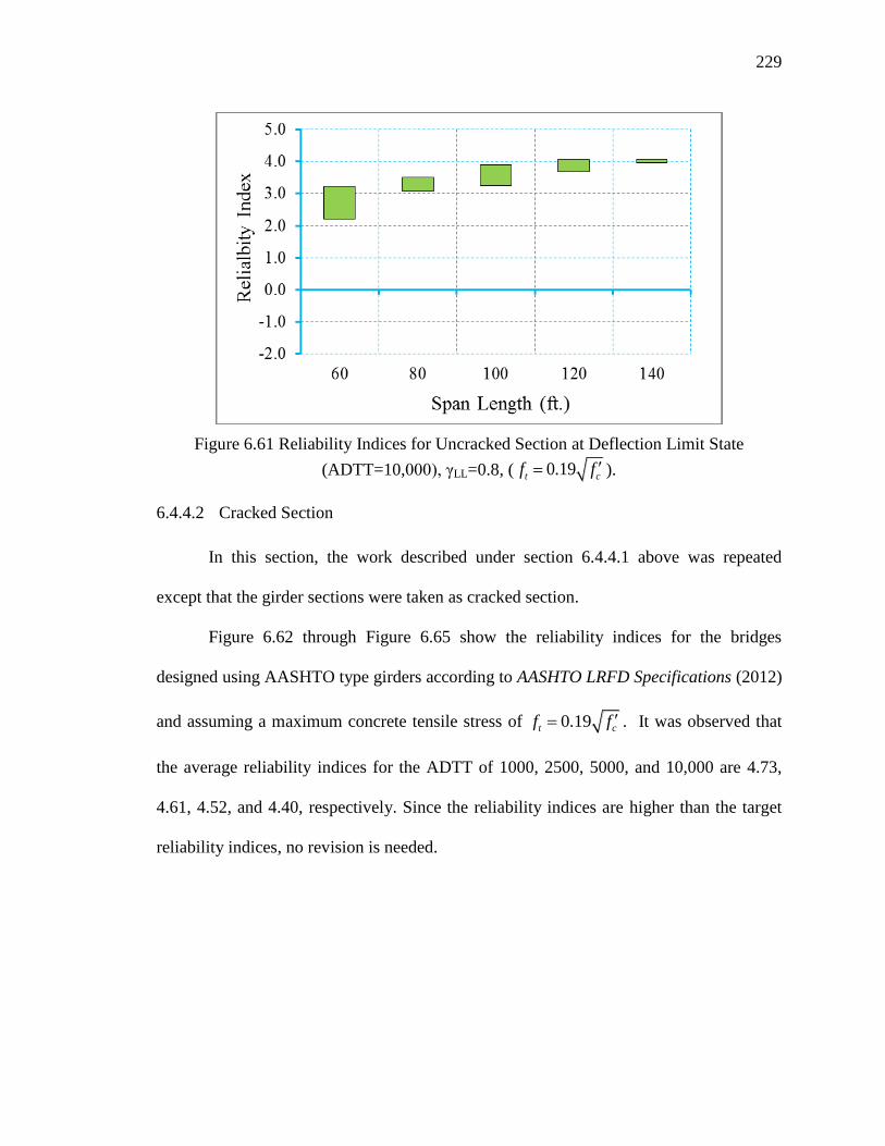
229
Figure 6.61 Reliability Indices for Uncracked Section at Deflection Limit State
(ADTT=10,000), γLL=0.8, ( 0.19t cf f ).
6.4.4.2 Cracked Section
In this section, the work described under section 6.4.4.1 above was repeated
except that the girder sections were taken as cracked section.
Figure 6.62 through Figure 6.65 show the reliability indices for the bridges
designed using AASHTO type girders according to AASHTO LRFD Specifications (2012)
and assuming a maximum concrete tensile stress of 0.19t cf f . It was observed that
the average reliability indices for the ADTT of 1000, 2500, 5000, and 10,000 are 4.73,
4.61, 4.52, and 4.40, respectively. Since the reliability indices are higher than the target
reliability indices, no revision is needed.

230
Figure 6.62 Reliability Indices for Cracked Section at Deflection Limit State
(ADTT=1000), γLL=0.8, ( 0.19t cf f ).
Figure 6.63 Reliability Indices for Cracked Section at Deflection Limit State
(ADTT=2500), γLL=0.8, ( 0.19t cf f ).

231
Figure 6.64 Reliability Indices for Cracked Section at Deflection Limit State
(ADTT=5000), γLL=0.8, ( 0.19t cf f ).
Figure 6.65 Reliability Indices for Cracked Section at Deflection Limit State
(ADTT=10,000), γLL=0.8, ( 0.19t cf f ).
232
7 SUMMARY AND CONCLUSIONS
CHAPTER 7
SUMMARY AND CONCLUSIONS
7.1 SUMMARY
In this study, various serviceability limit states have been developed and
investigated, including Service I limit state which is used for crack control of reinforced
concrete and Service III limit state which is used for tension at the bottom of prestressed
concrete girders. Extensive databases were developed for both Service I and Service III
limit state. The databases included the existing structures as well as simulated structures
with various design parameters been considered. These parameters include material
properties, geometrical parameters, and design exposure conditions. Models for
resistance and load were developed for both Service I and Service III limit state. Based
on the developed resistance and load models, the limit states were formulated and
reliability analysis was performed. Aiming at improving the level and uniformity of
reliability for various serviceability limit state, the design provisions were revised and the
effects of the changes was investigated. New design provisions are proposed to be
included in AASHTO LRFD Design Specification and to be used in future practice.
Furthermore, due to the fact the structural resistance would decrease because of
deterioration of the material strength and structure section, the effect of resistance
deterioration on reliability of structure at serviceability limit state was investigated.

233
7.2 PROPOSED REVISION IN AASHTO LRFD SPECIFICATION
As shown in previous Chapters, inconsistent reliability was observed for some
scenarios if using the provisions in current AASHTO LRFD Bridge Design Specification
(AASHTO, 2012). For instance, the bridge decks designed using the empirical method
based on current AASHTO LRFD Bridge Design Specification demonstrates insufficient
reliability level regarding the crack control limit state. Therefore, aiming at achieving
uniform reliability over different designs, the following revisions are proposed to be
included in AASHTO LRFD Bridge Design Specification.
7.2.1 Service I Limit State
The following revisions are proposed for Service I limit state regarding crack
control of reinforced concrete members.
(1) It is recommended that the ratio of the reinforcement area to section gross area
be increased from 0.3% to 0.4% for bottom layer and 0.2% to 0.5% for top
layer.
(2) No revisions to the live load factor for Service I limit state.
7.2.2 Service III Limit State
The following revisions are proposed for Service III limit state regarding tension
at tensile fibers of prestressed concrete members.
(1) Live load factor of 1.0 for Service III limit state.
234
(2) Maximum concrete tensile stress of 0.0948t cf f and 0.19t cf f for
bridges in severe corrosion conditions and for bridges in no worse than
moderate corrosion conditions, respectively.
(3) Girders to be designed following conventional design methods and assuming
the live loads exist in single lane or multiple lanes, whichever produces higher
load effects. The appropriate multiple presence factor applies.
7.3 CONCLUSIONS
The following conclusions are based on the findings of this work:
(1) The resistance of prestressed concrete girder at Service III limit state
regarding the tension at tensile fibers could be derived using structural
analysis for various performance levels named decompression, maximum
allowable tensile stress limit, and maximum allowable crack width.
(2) The statistical model for structural resistance and dead load can be obtained
using derived prediction equation and Monte-Carlo simulation techniques.
(3) A precise crack width prediction equation is important to provide an accurate
estimation of structural resistance, for Service I limit state, as well as for
Service III limit state at maximum allowable crack width level.
(4) Utilizing appropriate deterioration model, the effects of deterioration on
structural reliability can be evaluated. The deterioration of structure can be
attributed to section losses due to corrosion, strength losses due to long term
effects (shrinkage and creep of concrete).

235
(5) Deterioration of structure has significant effects on structural reliability at
both Service I and Service III limit state, especially for longer durations (e.g.
50 years, 75 years). Therefore, the deterioration of structure should be
considered for structural reliability analysis, especially for evaluation of long
term reliability of structure.
(6) WIM data must be processed to remove erroneous data, light vehicles, and
permit vehicles (if needed) before used for developing live load model.
(7) The live load for permit vehicles can be developed based on issued permit
data and statistics of actual permit vehicles.
(8) No revision is needed to be added to AASHTO LRFD Bridge Design
Specification for reinforced concrete deck designed using traditional design
method.
(9) No revision is needed to be added to AASHTO LRFD Bridge Design
Specification for deflection limit state for prestressed concrete girder.
(10) The reliability level of reinforced concrete deck designed using empirical
deck is lower than target reliability index, for both positive moment and
negative moment region. Therefore, the design provisions in current
AASHTO LRFD Bridge Design Specifications need to be modified.
(11) For a specific girder of known cross-section and specific number and
arrangement of prestressing strands, the reliability index varies based on: (a)
The design maximum concrete tensile stress (currently in the AASHTO LRFD
maximum tensile stress of 0.0948t cf f and 0.19t cf f ), (b) The limit
state function, i.e. decompression, tensile stress of a certain value (assumed to
236
be 0.19t cf f in the work shown above) or a crack width of a certain value
(assumed to be 0.016) and (c)ADTT.
(12) The target reliability index can be achieved uniformly across various span
lengths using the load factor developed following the procedure developed in
this study. The level of uniformity varies with the limiting criteria. The
decompression limit state showed the highest level of uniformity and is
recommended to be used as the basis for the reliability analysis, i.e. the
determination of the load and resistance factors and associated design criteria.
(13) It is recommended that the reliability indices corresponding to ADTT of
5000 be used as the basis for the calibration. The reliability index is not
highly sensitive to changes in the ADTT so there is no need for using different
load factor for ADTT’s up to 10000.
(14) With satisfactory past performance of prestressed beams, the target reliability
index is selected to be similar to the average inherent reliability index of the
bridges on the system. There is no scientific reason to substantiate targeting a
different, higher or lower, reliability index.
(15) The recommended target reliability index for the decompression limit state is
1.0 for bridges designed for no worse than moderate corrosion conditions and
1.2 for bridges designed for severe corrosion conditions. Based on the study
of WIM data, the reliability index is determined assuming live load exists in
single lane and without applying the multiple presence factor. This would
appear on the “load side” of the limit state function.
237
REFERENCES
AASHTO (2004). “LRFD bridge design specifications”, American Society of State
Highway and Transportation Officials (AASHTO), Washington, D.C.
Agarwal, A. C. and Wolkowicz, M. (1976). "Interim Report on 1975 Commercial
Vehicle Survey," Res. and Dev. Div., Ministry of Transportation, Downsview, Ontario,
Canada.
American Society for Testing and Materials, ASTM (1985). “E1049-85, Standard
practices for cycle counting in fatigue analysis.”
American Society for Testing and Materials, ASTM (2002). “E1318-02, Standard
Specification for Highway Weigh-in-Motion (WIM) Systems with User Requirements
and Test Methods.”
Ang, A. H.-S., and Tang, W.H. (1975). Probability Concepts in Engineering Planning
and Design: Volume I. Basic Principles. New York: Wiley.
Ang, A. H.-S., and Tang, W.H. (1984). Probability Concepts in Engineering Planning
and Design: Volume II. Decision, Risk, and Reliability. New York: Wiley.
Atlantic Trailer Company (2004), website: http://www.atlantictrailers.com
Bannantine, J.A., Comer, J.J., and Handrock, J.L. (1990). Fundamentals of Metal Fatigue
Analysis. Prentice Hall, Englewood Cliffs, NJ.
Bakht, B. and Jaeger, L. G. (1985). Bridge Analysis Simplified. McGraw-Hill:New York
Barker, R. M., J. M. Duncan, K.B. Rojiani, P. S. K. Ooi, C. K. Tan, and S. G. Kim
(1991). Manual for the Design of Bridge Foundations, NCHRP Report 343,
Transportation Research Board, Washington, DC, 308 pp.
Barker, R.M. and Puckett, J.A. (1997). Design of highway bridges: based on AASHTO
LRFD Bridge Design Specifications. New York: Wiley.
Brodtkorb, P.A., Johannesson, P., Lindgren, G., Rychlik, I., Ryden, J., and Sjo, E.
(2000). “WAFO – A Matlab toolbox for analysis of random waves and loads.”
Norwegian University of Science and Technology, Lund Institute of Technology.
Chen, Y. (1994). "Modeling Bridges Subjected to Moving Loads," Mathematical
Modeling and Scientific Computing, Vol. 4, pp 567-572.

238
Coles, S. (2001). "An Introduction to Statistical Modeling of Extreme Values".
Springer-Verlag, London.
Dressler, K., Hack, M., Krueger, W. (1997). “Stochastic reconstruction of loading
histories from a rainflow matrix.” Zeit. F. ang. Math. U. Mech. 77(3), pp 217-226.
Dressler, K., Gründer, B., Hack, M., and Köttgen, V.B. (1996). “Extrapolation of
Rainflow Matrices.” SAE Technical Paper 960569.
Downing, S.D. and Socie, D.F. (1982). “Simple rainflow counting algorithms.”
International Journal of Fatigue, 4(1), pp 31-40.
Federal Highway Administration, FHWA (2001). “FHWA Vehicle Types,” USDOT
online: http://www.fhwa.dot.gov/policy/ohpi/vehclass.htm
Federal Highway Administration, FHWA (2006). “Bridge Formula,” USDOT online:
http://www.fhwa.dot.gov/policy/ohpi/vehclass.htm
Fisher, J.W., Mertz, D.R., and Zhong, A. (1983) “Steel bridge members under variable
amplitude long life fatigue loading.” National Cooperative Highway Research Program
Report 267.
Fisher, J.W., Jian, J., Wagner, D.C., and Yen, B.T. (1990). “Distortion-induced fatigue
cracking in steel bridges.” National Cooperative Highway Research Program Report
336.
Fisher, J.W., G.L Kulak, and I.F. Smith (1998) “A Faitgue Primer for Structural
Engineers.” National Steel Bridge Alliance, American Institute of Steel Construction.
Fu, G., Feng, J., Dekelbab, W., Moses, F., Cohen, H., Mertz, D., and Thompson, P.
Effect of Truck Weight on Bridge Network Costs. NCHRP Report 495. Transportation
Research Board. Washington D.C., 2003.
Hahin, C., South, J.M., Mohammadi, J., and Polpeddi, R.K. (1993). “Accurate and Rapid
Determination of Fatigue Damage in Steel Bridges.” Journal of Structural Engineering.
ASCE, 119(1), 150-168.
International Road Dynamics Inc. (1999), “Software User’s Manual: IRD Weigh-In-
Motion Data Collection System,” Version 7.5.0, December.
International Road Dynamics Inc. (2005), “Operator’s Manual-TC/C 540,” Revision C,
Part No. 69004801, January.
Jaeger, L. G. and Bakht, B. (1982). "The Grillage Analogy in Bridge Analysis,"
Canadian Journal of Civil Engineering, Vol. 9, pp. 224-235.
239
Jaeger, L.G. and Bahkt, B. (1989). Bridge Analysis by Microcomputer. McGraw-Hill
Co., New York.
Johannesson, P., Thomas, J-J. (2001). “Extrapolation of rainflow matrices.” Extremes,
4(3), 241-262.
Khosrovaneh, A.K. and Dowling, N.E. (1990). “Fatigue loading history reconstruction
based on the rainflow technique.” International Journal of Fatigue, 12(2), pp 99-106.
Laman, J. and Nowak, A. (1996). “Fatigue-load model for girder bridges.” Journal of
Structural Engineering, ASCE, 122(7), pp726-733.
Liu, M. (1996). "A Three-Dimensional Dynamic Model for Bridge-Road-Vehicle
System," Master's Thesis, Bradley University, Peoria, IL.
Manitowok Crane Group (2006). “Specifications for Grove portable cranes” online:
http://www.manitowokcranegroup.com
MATLAB (2000), The Language of Technical Computing, Version 6.0, Release 12, The
MathWorks, Inc., MA.
Matsuishi, M. and Endo, T. (1968). “Fatigue of metals subjected to varying stress-
fatigue lives under random loading.” Preliminary Proceedings of the Kyushu District
Meeting, pages 37-40. The Japan Society of Mechanical Engineers. In Japanese, March
1968.
Microsoft Terraserver Aerial Photographs (2005), http://terraserver.microsoft.com
Microsoft Virtual Earth (2007). http://live.local.com
Mohammadi, J., Guralnick, S.A., and Polepeddi, R. (1998). “Bridge fatigue life
estimation from field data.” Practice Periodical on Structural Design and Construction,
3(3), 128-133.
Mohammadi, J., and Polepeddi, R. (2000). “Bridge rating with consideration for fatigue
damage from overloads.” Journal of Bridge Engineering, ASCE, 5(3), 259-265.
Moses, F. (2001) “Calibration of Load Factors for LRFR Bridge Evaluation,” NCHRP
Report 454, Transportation Research Board, National Research Council, Washington,
D.C.
Moses, F., Schilling, C.G., and Raju, K.S. (1987) “Fatigue evaluation procedures for
steel bridges.” National Cooperative Highway Research Program Report 299.
Munse, W.H. (1990). “Fatigue, brittle fracture, and lamellar tearing.” Structural
engineering handbook, 3rd
Ed. E.H. Gaylord Jr. and C.N. Gaylord, eds., McGraw-Hill
Inc., N.Y., 4.1-4.24.

240
Nassif, H. H., Gindy, M. and Davis, J. (2005). “Monitoring of Bridge Girder Deflection
Using Laser Doppler Vibrometer,” Journal of Non-Destructive Testing and Evaluation,
38,
Nassif, H. H. and Liu, M. (2004). "Analytical Modeling of Bridge-Road-Vehicle
Dynamic Interaction System," Journal of Vibration and Control, Vol. 10, pp. 215-241.
Nassif, H. H., Liu, M. and Ertekin, O. (2003). "Model Validation for Bridge-Road-
Vehicle Dynamic Interaction System," Journal of Bridge Engineering, Vol. 8, No. 2,
pp.112-120.
New Jersey Department of Transportation, NJDOT (2002), Bridges and Structures
Design Manual, 2002 available online at http://www.state.nj.us/transportation/
New Jersey Department of Transportation, NJDOT (2005), email correspondence with
Research Bureau, Dec 2005.
Nowak, A. S. and Lind, N. C. (1979). “Practical bridge code calibration.” Journal of the
Structural Division, ASCE, 105(12), 2497-2510, Dec.
Nowak, A.S., Nassif, H.N., and DeFrain, L. (1993). “Effect of truck loads on bridges.”
Journal of Transportation Engineering. 119(6), 853-867.
Nowak, A.S., Nassif, N., and Frank, K.H. (1993). “Fatigue Load Spectra for a Steel
Girder Bridge.” Transportation Research Record 1393, pp. 154-161.
Nowak, A.S., Nassif, H., and Frank, K.H. (1993). “Fatigue load spectra for a steel girder
bridge.” Transportation Research Record 1393, Transportation Research Board,
Washington, D.C.
Nowak, A.S. (1995). “Calibration of the LRFD bridge code.” Journal of Structural
Engineering. ASCE, 121(8), 1245-1251
Nowak, A.S. (1999). “Calibration of the LRFD Bridge Design Code.” NCHRP Report
368, Transportation Research Board, National Research Council, Washington, D.C.
Nowak, A. S. and Collins, K. R. (2000). "Reliability of Structures". McGraw Hill
Companies, Inc.
Nowak, A. S. and Hong, Y. K. (1991). “Bridge Live-Load Models," Journal of
Structural Engineering, ASCE, 117(9), pp. 2757-2767.
Phuvoravan, K., W. Chung, J. Liu, and E.D. Sotelino, (2004). “Simplified Live-Load
Distribution Factor Equations for Steel Girder Bridges,” Transportation Research
241
Record: Journal of the Transportation Research Board, No. 1892, National Research
Council, Washington, D.C., pp. 88-97.
Port Authority of New York and New Jersey, PANYNJ (2005). “Freight volumes study
2005” available online: htpp://www.panynj.gov
Schilling, C.G., et al. (1978). “Fatigue of welded steel bridge members under variable-
amplitude loadings.” NCHRP Report 188.
Socie, D. (2001). “Modeling expected service usage from short term loading
measurements.” International Journal of Materials & Product Technology, 16(4/5).
Socie, D.F. and Pompetzki, M.A. (2004). “Modeling variability in service loading
spectra.” Journal of ASTM International, 1(2), Paper ID JAI11561, Feb. 2004.
Southgate, H. (2000). “Quality Assurance of Weigh-in-motion Data” FHWA Contract
No. DTFH61-P-00724. Federal Highway Administration USDOT, Washington D.C.
Thoft-Christensen, P. and Baker, M. J., Structural Reliability Theory and Its
Applications. Springer-Verlag, 1982.
West, R. (1973). "Recommendations on the Use of Grillage Analysis for Slab and
Pseudo-slab Bridge Decks," Cement and Concrete Association and Construction Industry
Research and Information Association, London, UK.
Zokaie, T., T.A. Osterkamp, and R.A. Imbsen (1991). Distribution of Wheel Loads on
Highway Bridges, Final Report Project 12-26/1, National Cooperative Highway Research
Program, Transportation Research Board, National Research Council, Washington, DC.
Park R., (1964) “Ultimate Strength of Rectangular Concrete Slabs under Short-term
Uniform Loading with Edges Restrained against Lateral Movement,” Proceedings of the
Institution of Civil Engineers, Structures and Buildings, V. 28, pp. 125-150.
Fang, I.-K., Worley, J., Klingner, R. E., and Burns, N. H., (1986) “Behavior of Ontario-
Type Bridge Decks on Steel Girders,” Research Report 350-1, Center for Transportation
Research, University of Texas at Austin, Austin, TX.
Tsui, C. K., Burns, N. H., and Klingner, R. E., (1986) “Behavior of Ontario-Type Bridge
Decks on Steel Girders: Negative Moment Region and Load Capacity,” Research Report
350-3, Center for Transportation Research, University of Texas at Austin, Austin, TX.
Guice, L. K. and Rhombery, E. J., (1988) “Membrane Action in Partially Restrained
Slabs,” ACI Structural Journal, Vol. 85, No. 4, p. 365-373.
242
Fang, I.-K., Worley, J., Burns, N. H., and Klingner, R. E., (1990a)“Behavior of Isotropic
R/C Bridge Decks on Steel Girders,” ,” ASCE, Journal of Structural Engineering. Vol.
116, No. 3, pp 659-678.
Fang, I.-K., Tsui, C. K., Burns, N. H., and Klingner, R. E., (1990b)“Fatigue Behavior of
Cast-in-Place and Precast Panel Bridge Decks with Isotropic Reinforcement,” PCI
Journal. May-June, pp 28-39.
Fang, I.-K., Tsui, C. K., Burns, N. H., and Klingner, R. E., (1990c)“Load Capacity of
Isotropically Reinforced, Cast-in-Place and Precast Panel Bridge Decks,” PCI Journal.
July-August, pp 104--113.
Fang, I.-K., Lee, J.-H., and Chen, C.-R., (1994) “Behavior of Partially Restrained Slabs
under Concentrated Load,” ACI Structural Journal. Vol. 91, No. 2, pp 133--139.
Rankin, G. I. B., and Long, A. E., (1997) “Arching Action Strength Enhancement in
Laterally- Restrained Slab Strips,” Proceedings of the Institution of Civil Engineers,
Structures and Buildings, V. 122, pp. 461-467.
Frosch, Robert J., (1999) “Another Look at Cracking and Crack Control in Reinforced
Concrete” ACI Structural Journal, Vol. 96, No. 3, p. 437.
Siriaksorn, A. and Naaman, A. E., Reliability of partially prestressed beams at
serviceability limit states, University of Illinois at Chicago Circle, Dept. of Materials
Engineering. Research Report, June 1980. 126 pp.
Peel-Cross, J., Rankin, G. I. B., Gilbert, S. G., and Long, A. E. (2000) “Compressive
Membrane Action in Composite Floor Slabs in the Cardington LBTF,” Proceedings of
the Institution of Civil Engineers, Structures and Buildings, V. 146, pp. 217-226.
Bailey, C. G., (2001) “Membrane Action of Unrestrained Lightly Reinforced Concrete
Slabs at Large Displacements,” Engineering Structures, V. 23, pp 470-483.
Graddy, J. C., Kim, J., Whitt, J. H., Burns, N. H., and Klingner, R. E. (2002), “Punching-
Shear Behavior of Bridge Decks under Fatigue Loading”, ACI Structural Journal, Vol.
99, pp 257-266.
Salim, W. and Sebastian, W. M. (2003) “Punching Shear Failure in Reinforced Concrete
Slabs with Compressive Membrane Action,” ACI Structural Journal, Vol. 100, pp 39-48.
Taylor, S. E., Rankin, B., and Cleland, D. J. (2003) “Real Strength of High-performance
Concrete Bridge Deck Slabs” Proceedings of the Institution of Civil Engineers. Issue
BE2 pp 81-90.

243
Taylor, S. E., Rankin, B., Cleland, D. J. and Kirkpatrick, J. (2007) “Serviceability of
Bridge Deck Slabs with Arching Action,” ACI Structural Journal, Vol. 104, pp 471-479.
Bailey, C. G., Toh, W. S., and Chan, B. K. (2008) “Simplified and Advanced Analysis of
Membrane Action of Concrete Slabs,” ACI Structural Journal, Vol. 105, pp 30-40.
Nowak, A. S., Szersen, M. M., Szeliga, E. K., Szwed, A., and Podhorecki, P. J. (2008),
“Reliability-Based Calibration for Structural Concrete, Phase 3” Portland Cement
Association and Precast/Prestressed Concrete Institute. PCA R&D Serial No.2849, 110
pp.
Meadway, J. M. (2008) “Evaluation of Current Deck Design Practices,” Master Thesis,
West Virginia University.
Taylor, S.E., Rankin, G. I. B., and Cleland, D. J. (2003), “Real Strength of High-
performance Concrete Bridge Deck Slabs,” Proceedings of the Institution of Civil
Engineers, Bridge Engineering, V. 156, pp. 81-90.
Mufti, A. and Hassan, T. (2005), “Finite Element Analysis and Theoretical Study of
Punching Shear Strength of Concrete Bridge Decks,” Canadian Journal of Civil
Engineering, V32, pp 449-453.
Hon, A., Taplin, G., Al-Mahaidi, R. S. (2005), “Strength of Reinforced Concrete Bridge
Decks under Compressive Membrane Action,” ACI Structural Journal, V102, pp 393-
401.
Schmeckpeper, E. R., Nielsen, R., Shiner, C., and Blandford, M. (2009), "the effect of
bridge deck design methodology on crack control," Research Report N09-08.
FDOT. (1999). “Corrosion evaluation of post-tensioned tendons on the Niles Channel
Bridge”. Florida Department of Transportation (FDOT), Tallahassee, Florida.
FDOT. (2001a). “Mid-Bay bridge post-tensioning evaluation”, final report. Washington
(DC): Corven Engineering, Inc., Florida Department of Transportation (FDOT),
Tallahassee, Florida.
FDOT. (2001b). “Sunshine skyway bridge post-tensioned tendons investigation”. Parsons
Brinckerhoff Quade and Douglas, Inc., Florida Department of Transportation (FDOT),
Tallahassee, Florida.
Hansen B. (2007). “Forensic engineering: tendon failure raises questions about grout in
post-tensioned bridges”. Civil Eng News;November:17-8.

244
Pillai, R. G., Hueste, M. D., Gardoni, P., Trejo, D., & Reinschmidt, K. F. (2010). Time-
variant service reliability of post-tensioned, segmental, concrete bridges exposed to
corrosive environments. Engineering Structures, 32(9), 2596-2605.
ACI Committee 209, (1997). Prediction of creep, shrinkage and temperature effects in
concrete structures, AC1 Manual of concrete practice, Part I, 209R 1-92.
Darmawan, M. S. and Stewart, M. G. (2007). Effect of pitting corrosion on capacity
of prestressing wires. Magazine of Concrete Research, Vol. 59, No. 2, pp. 131–139.
Zandi Hanjari, K. (2010). Structural behaviour of deteriorated concrete structures.
Chalmers University of Technology.
Akgül, F., & Frangopol, D. M. (2004). Time-dependent interaction between load rating
and reliability of deteriorating bridges. Engineering structures, 26(12), 1751-1765.

245
APPENDIX A. BRIDGE DATABASES
APPENDIX A
BRIDGE DATABASES
In order to develop a comprehensive limit state, a broad bridge database that
covers various design criteria and various design conditions is required. Therefore,
bridge databases were developed for various girder types that used in current practice,
includes AASHTO I Girders, AASHTO Adjacent Box Girders, AASHTO Spread Box
Girders, and AASHTO ASBI Large Box Girders. For each girder type, a set of bridges
were designed for span lengths ranging from 30 ft to 160 ft, except for AASHTO ASBI
Large Box Girders, which were designed for span lengths ranging from 100 ft to 200 ft.
Various design criteria such as live load factor, prestress losses calculation method, and
maximum allowable tensile stress were also considered for each girder type.
Furthermore, databases of existing bridges from NCHRP Project 12-78 were also
included in this study for the investigation of reliability level of existing bridges. The
databases for existing bridges contains I girders, spread box girders and adjacent box
girders.
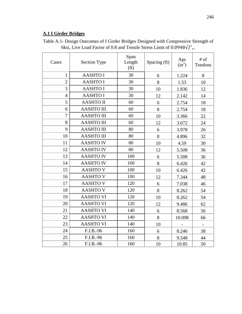
246
A.1 I Girder Bridges
Table A.1- Design Outcomes of I Girder Bridges Designed with Compressive Strength of
6ksi, Live Load Factor of 0.8 and Tensile Stress Limit of .
Cases Section Type
Span
Length
(ft)
Spacing (ft) Aps
(in2)
# of
Tendons
1 AASHTO I 30 6 1.224 8
2 AASHTO I 30 8 1.53 10
3 AASHTO I 30 10 1.836 12
4 AASHTO I 30 12 2.142 14
5 AASHTO II 60 6 2.754 18
6 AASHTO III 60 8 2.754 18
7 AASHTO III 60 10 3.366 22
8 AASHTO III 60 12 3.672 24
9 AASHTO III 80 6 3.978 26
10 AASHTO III 80 8 4.896 32
11 AASHTO IV 80 10 4.59 30
12 AASHTO IV 80 12 5.508 36
13 AASHTO IV 100 6 5.508 36
14 AASHTO IV 100 8 6.426 42
15 AASHTO V 100 10 6.426 42
16 AASHTO V 100 12 7.344 48
17 AASHTO V 120 6 7.038 46
18 AASHTO V 120 8 8.262 54
19 AASHTO VI 120 10 8.262 54
20 AASHTO VI 120 12 9.486 62
21 AASHTO VI 140 6 8.568 56
22 AASHTO VI 140 8 10.098 66
23 AASHTO VI 140 10 - -
24 F.I.B.-96 160 6 8.246 38
25 F.I.B.-96 160 8 9.548 44
26 F.I.B.-96 160 10 10.85 50

247
Table A.2- Design Outcomes of I Girder Bridges Designed with Compressive Strength of
6ksi, Live Load Factor of 0.8 and Tensile Stress Limit of 0.158 .
Cases Section Type
Span
Length
(ft)
Spacing (ft) Aps
(in2)
# of
Tendons
1 AASHTO I 30 6 1.224 8
2 AASHTO I 30 8 1.53 10
3 AASHTO I 30 10 1.53 10
4 AASHTO I 30 12 1.836 12
5 AASHTO II 60 6 2.448 16
6 AASHTO III 60 8 2.448 16
7 AASHTO III 60 10 3.06 20
8 AASHTO III 60 12 3.366 22
9 AASHTO III 80 6 3.672 24
10 AASHTO IV 80 8 3.978 26
11 AASHTO IV 80 10 4.284 28
12 AASHTO IV 80 12 4.896 32
13 AASHTO IV 100 6 5.202 34
14 AASHTO IV 100 8 6.12 40
15 AASHTO V 100 10 5.814 38
16 AASHTO V 100 12 6.732 44
17 AASHTO V 120 6 6.426 42
18 AASHTO V 120 8 7.65 50
19 AASHTO VI 120 10 7.65 50
20 AASHTO VI 120 12 8.874 58
21 AASHTO VI 140 6 7.956 52
22 AASHTO VI 140 8 9.792 64
23 AASHTO VI 140 10 - -
24 F.I.B.-96 160 6 7.378 34
25 F.I.B.-96 160 8 8.68 40
26 F.I.B.-96 160 10 10.416 48

248
Table A.3- Design Outcomes of I Girder Bridges Designed with Compressive Strength of
6ksi, Live Load Factor of 0.8 and Tensile Stress Limit of .
Cases Section Type
Span
Length
(ft)
Spacing (ft) Aps
(in2)
# of
Tendons
1 AASHTO I 30 6 1.224 8
2 AASHTO I 30 8 1.53 10
3 AASHTO I 30 10 1.836 12
4 AASHTO I 30 12 2.142 14
5 AASHTO II 60 6 2.448 16
6 AASHTO III 60 8 2.142 14
7 AASHTO III 60 10 2.754 18
8 AASHTO III 60 12 3.366 22
9 AASHTO III 80 6 3.366 22
10 AASHTO III 80 8 4.59 30
11 AASHTO IV 80 10 4.284 28
12 AASHTO IV 80 12 4.896 32
13 AASHTO IV 100 6 4.896 32
14 AASHTO IV 100 8 6.12 40
15 AASHTO V 100 10 5.814 38
16 AASHTO V 100 12 6.732 44
17 AASHTO V 120 6 6.12 40
18 AASHTO V 120 8 7.65 50
19 AASHTO VI 120 10 7.344 48
20 AASHTO VI 120 12 8.568 56
21 AASHTO VI 140 6 7.65 50
22 AASHTO VI 140 8 9.18 60
23 AASHTO VI 140 10 - -
24 F.I.B.-96 160 6 7.378 34
25 F.I.B.-96 160 8 8.68 40
26 F.I.B.-96 160 10 9.982 46
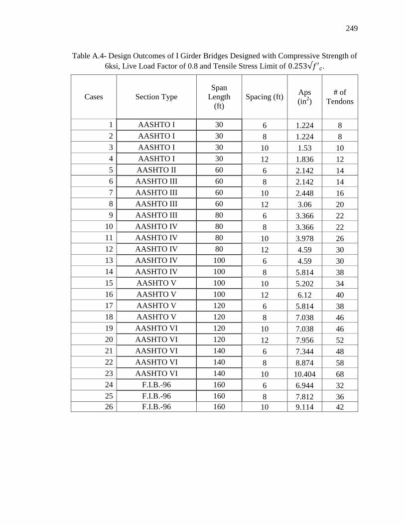
249
Table A.4- Design Outcomes of I Girder Bridges Designed with Compressive Strength of
6ksi, Live Load Factor of 0.8 and Tensile Stress Limit of .
Cases Section Type
Span
Length
(ft)
Spacing (ft) Aps
(in2)
# of
Tendons
1 AASHTO I 30 6 1.224 8
2 AASHTO I 30 8 1.224 8
3 AASHTO I 30 10 1.53 10
4 AASHTO I 30 12 1.836 12
5 AASHTO II 60 6 2.142 14
6 AASHTO III 60 8 2.142 14
7 AASHTO III 60 10 2.448 16
8 AASHTO III 60 12 3.06 20
9 AASHTO III 80 6 3.366 22
10 AASHTO IV 80 8 3.366 22
11 AASHTO IV 80 10 3.978 26
12 AASHTO IV 80 12 4.59 30
13 AASHTO IV 100 6 4.59 30
14 AASHTO IV 100 8 5.814 38
15 AASHTO V 100 10 5.202 34
16 AASHTO V 100 12 6.12 40
17 AASHTO V 120 6 5.814 38
18 AASHTO V 120 8 7.038 46
19 AASHTO VI 120 10 7.038 46
20 AASHTO VI 120 12 7.956 52
21 AASHTO VI 140 6 7.344 48
22 AASHTO VI 140 8 8.874 58
23 AASHTO VI 140 10 10.404 68
24 F.I.B.-96 160 6 6.944 32
25 F.I.B.-96 160 8 7.812 36
26 F.I.B.-96 160 10 9.114 42
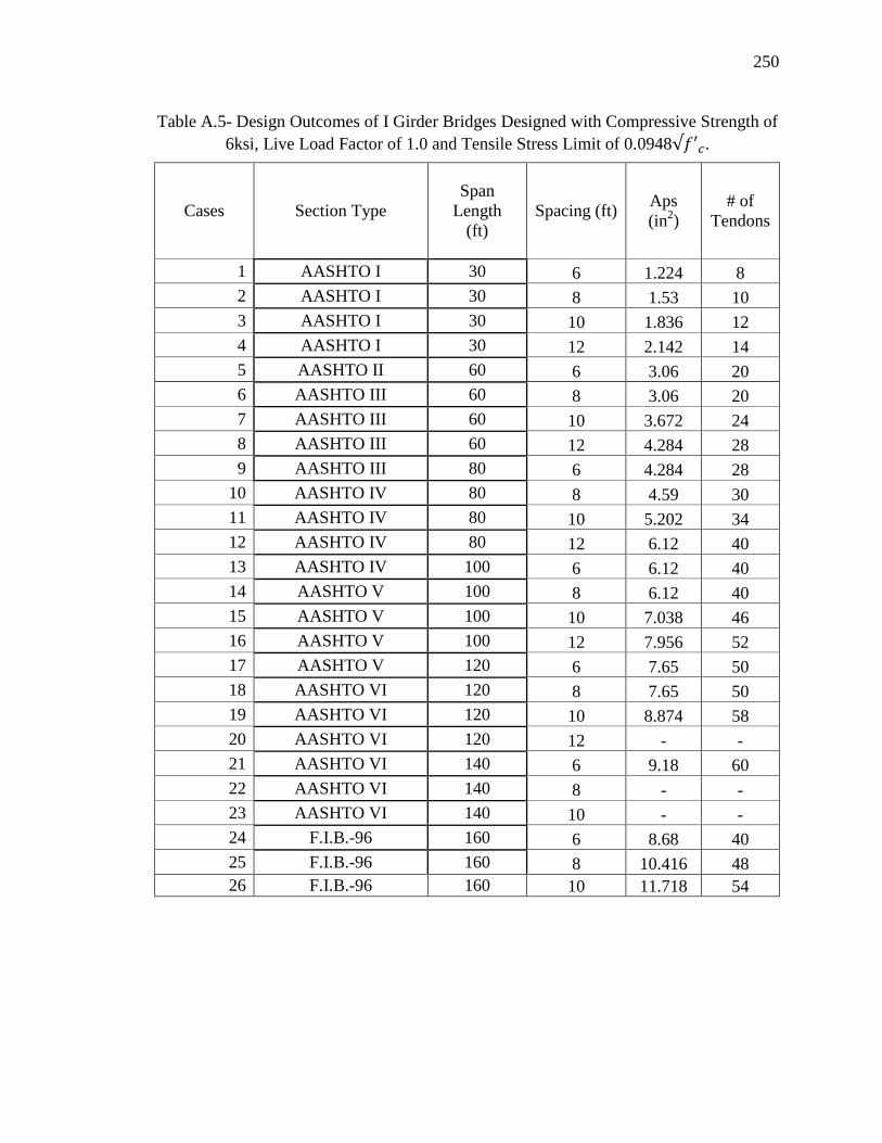
250
Table A.5- Design Outcomes of I Girder Bridges Designed with Compressive Strength of
6ksi, Live Load Factor of 1.0 and Tensile Stress Limit of 0.0948 .
Cases Section Type
Span
Length
(ft)
Spacing (ft) Aps
(in2)
# of
Tendons
1 AASHTO I 30 6 1.224 8
2 AASHTO I 30 8 1.53 10
3 AASHTO I 30 10 1.836 12
4 AASHTO I 30 12 2.142 14
5 AASHTO II 60 6 3.06 20
6 AASHTO III 60 8 3.06 20
7 AASHTO III 60 10 3.672 24
8 AASHTO III 60 12 4.284 28
9 AASHTO III 80 6 4.284 28
10 AASHTO IV 80 8 4.59 30
11 AASHTO IV 80 10 5.202 34
12 AASHTO IV 80 12 6.12 40
13 AASHTO IV 100 6 6.12 40
14 AASHTO V 100 8 6.12 40
15 AASHTO V 100 10 7.038 46
16 AASHTO V 100 12 7.956 52
17 AASHTO V 120 6 7.65 50
18 AASHTO VI 120 8 7.65 50
19 AASHTO VI 120 10 8.874 58
20 AASHTO VI 120 12 - -
21 AASHTO VI 140 6 9.18 60
22 AASHTO VI 140 8 - -
23 AASHTO VI 140 10 - -
24 F.I.B.-96 160 6 8.68 40
25 F.I.B.-96 160 8 10.416 48
26 F.I.B.-96 160 10 11.718 54
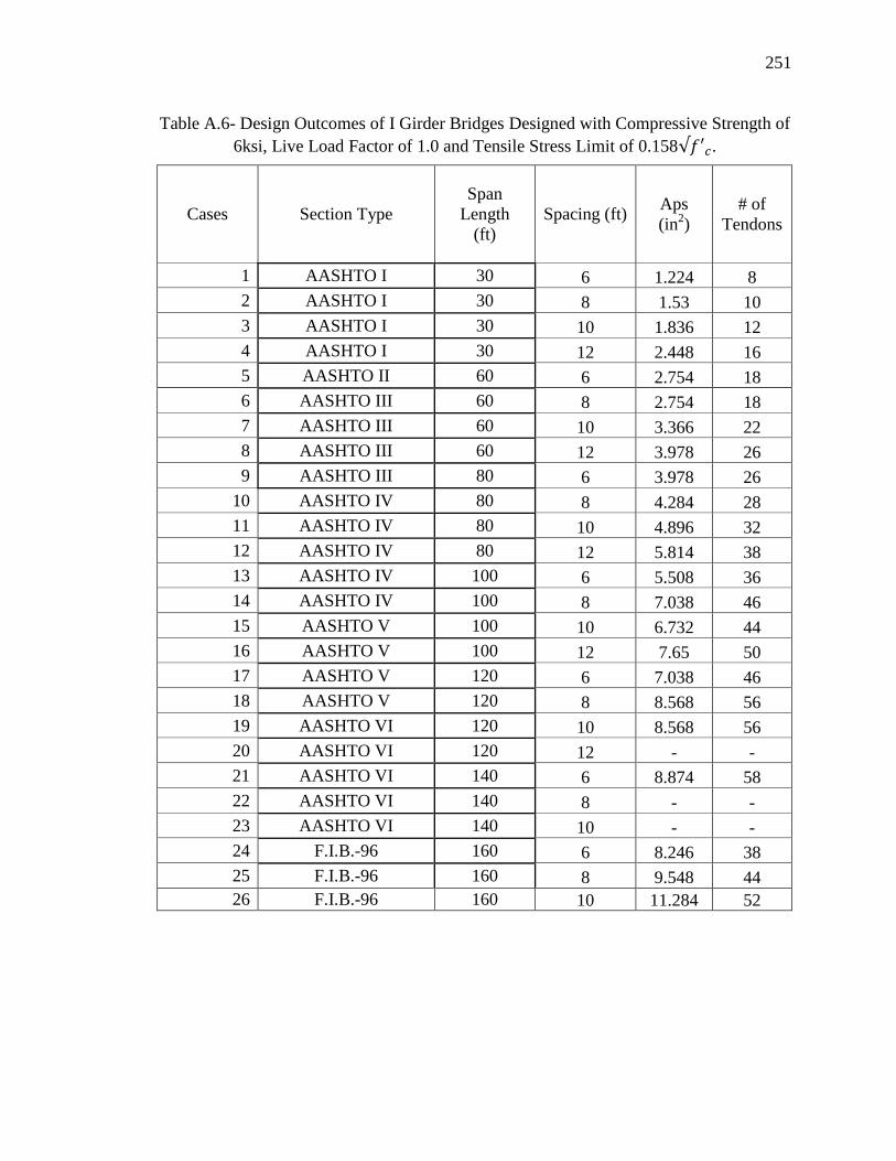
251
Table A.6- Design Outcomes of I Girder Bridges Designed with Compressive Strength of
6ksi, Live Load Factor of 1.0 and Tensile Stress Limit of 0.158 .
Cases Section Type
Span
Length
(ft)
Spacing (ft) Aps
(in2)
# of
Tendons
1 AASHTO I 30 6 1.224 8
2 AASHTO I 30 8 1.53 10
3 AASHTO I 30 10 1.836 12
4 AASHTO I 30 12 2.448 16
5 AASHTO II 60 6 2.754 18
6 AASHTO III 60 8 2.754 18
7 AASHTO III 60 10 3.366 22
8 AASHTO III 60 12 3.978 26
9 AASHTO III 80 6 3.978 26
10 AASHTO IV 80 8 4.284 28
11 AASHTO IV 80 10 4.896 32
12 AASHTO IV 80 12 5.814 38
13 AASHTO IV 100 6 5.508 36
14 AASHTO IV 100 8 7.038 46
15 AASHTO V 100 10 6.732 44
16 AASHTO V 100 12 7.65 50
17 AASHTO V 120 6 7.038 46
18 AASHTO V 120 8 8.568 56
19 AASHTO VI 120 10 8.568 56
20 AASHTO VI 120 12 - -
21 AASHTO VI 140 6 8.874 58
22 AASHTO VI 140 8 - -
23 AASHTO VI 140 10 - -
24 F.I.B.-96 160 6 8.246 38
25 F.I.B.-96 160 8 9.548 44
26 F.I.B.-96 160 10 11.284 52
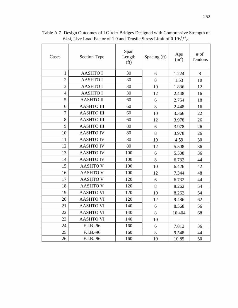
252
Table A.7- Design Outcomes of I Girder Bridges Designed with Compressive Strength of
6ksi, Live Load Factor of 1.0 and Tensile Stress Limit of 0.19 .
Cases Section Type
Span
Length
(ft)
Spacing (ft) Aps
(in2)
# of
Tendons
1 AASHTO I 30 6 1.224 8
2 AASHTO I 30 8 1.53 10
3 AASHTO I 30 10 1.836 12
4 AASHTO I 30 12 2.448 16
5 AASHTO II 60 6 2.754 18
6 AASHTO III 60 8 2.448 16
7 AASHTO III 60 10 3.366 22
8 AASHTO III 60 12 3.978 26
9 AASHTO III 80 6 3.978 26
10 AASHTO IV 80 8 3.978 26
11 AASHTO IV 80 10 4.59 30
12 AASHTO IV 80 12 5.508 36
13 AASHTO IV 100 6 5.508 36
14 AASHTO IV 100 8 6.732 44
15 AASHTO V 100 10 6.426 42
16 AASHTO V 100 12 7.344 48
17 AASHTO V 120 6 6.732 44
18 AASHTO V 120 8 8.262 54
19 AASHTO VI 120 10 8.262 54
20 AASHTO VI 120 12 9.486 62
21 AASHTO VI 140 6 8.568 56
22 AASHTO VI 140 8 10.404 68
23 AASHTO VI 140 10 - -
24 F.I.B.-96 160 6 7.812 36
25 F.I.B.-96 160 8 9.548 44
26 F.I.B.-96 160 10 10.85 50

253
Table A.8- Design Outcomes of I Girder Bridges Designed with Compressive Strength of
6ksi, Live Load Factor of 1.0 and Tensile Stress Limit of 0.253 .
Cases Section Type
Span
Length
(ft)
Spacing (ft) Aps
(in2)
# of
Tendons
1 AASHTO I 30 6 1.224 8
2 AASHTO I 30 8 1.224 8
3 AASHTO I 30 10 1.53 10
4 AASHTO I 30 12 1.836 12
5 AASHTO II 60 6 2.448 16
6 AASHTO III 60 8 2.448 16
7 AASHTO III 60 10 3.06 20
8 AASHTO III 60 12 3.672 24
9 AASHTO III 80 6 3.672 24
10 AASHTO IV 80 8 3.672 24
11 AASHTO IV 80 10 4.284 28
12 AASHTO IV 80 12 5.202 34
13 AASHTO IV 100 6 5.202 34
14 AASHTO IV 100 8 6.426 42
15 AASHTO V 100 10 5.814 38
16 AASHTO V 100 12 7.038 46
17 AASHTO V 120 6 6.426 42
18 AASHTO V 120 8 7.956 52
19 AASHTO VI 120 10 7.65 50
20 AASHTO VI 120 12 8.874 58
21 AASHTO VI 140 6 7.956 52
22 AASHTO VI 140 8 9.792 64
23 AASHTO VI 140 10 - -
24 F.I.B.-96 160 6 7.378 34
25 F.I.B.-96 160 8 8.68 40
26 F.I.B.-96 160 10 10.416 48

254
Table A.9- Design Outcomes of I Girder Bridges Designed with Compressive Strength of
8ksi, Live Load Factor of 0.8 and Tensile Stress Limit of 0.0948 .
Cases Section Type
Span
Length
(ft)
Spacing (ft) Aps
(in2)
# of
Tendons
1 AASHTO I 30 6 1.224 8
2 AASHTO I 30 8 1.53 10
3 AASHTO I 30 10 1.836 12
4 AASHTO I 30 12 1.836 12
5 AASHTO II 60 6 2.448 16
6 AASHTO II 60 8 3.366 22
7 AASHTO III 60 10 3.06 20
8 AASHTO III 60 12 3.672 24
9 AASHTO III 80 6 3.672 24
10 AASHTO III 80 8 4.59 30
11 AASHTO III 80 10 5.508 36
12 AASHTO IV 80 12 5.202 34
13 AASHTO III 100 6 6.12 40
14 AASHTO IV 100 8 6.426 42
15 AASHTO IV 100 10 7.344 48
16 AASHTO V 100 12 7.038 46
17 AASHTO IV 120 6 7.956 52
18 AASHTO V 120 8 7.956 52
19 AASHTO V 120 10 9.18 60
20 AASHTO VI 120 12 8.874 58
21 AASHTO VI 140 6 8.262 54
22 AASHTO VI 140 8 9.792 64
23 AASHTO VI 140 10 11.322 74
24 F.I.B.-96 160 6 7.812 36
25 F.I.B.-96 160 8 9.114 42
26 F.I.B.-96 160 10 10.416 48

255
Table A.10- Design Outcomes of I Girder Bridges Designed with Compressive Strength
of 8ksi, Live Load Factor of 0.8 and Tensile Stress Limit of 0.158 .
Cases Section Type
Span
Length
(ft)
Spacing (ft) Aps
(in2)
# of
Tendons
1 AASHTO I 30 6 1.224 8
2 AASHTO I 30 8 1.53 10
3 AASHTO I 30 10 1.836 12
4 AASHTO I 30 12 2.295 15
5 AASHTO II 60 6 2.448 16
6 AASHTO II 60 8 3.672 24
7 AASHTO III 60 10 3.06 20
8 AASHTO III 60 12 3.672 24
9 AASHTO III 80 6 3.366 22
10 AASHTO III 80 8 4.284 28
11 AASHTO III 80 10 5.202 34
12 AASHTO IV 80 12 4.896 32
13 AASHTO III 100 6 5.814 38
14 AASHTO IV 100 8 5.814 38
15 AASHTO IV 100 10 7.038 46
16 AASHTO V 100 12 6.426 42
17 AASHTO IV 120 6 7.344 48
18 AASHTO V 120 8 7.344 48
19 AASHTO V 120 10 8.568 56
20 AASHTO VI 120 12 8.262 54
21 AASHTO VI 140 6 7.65 50
22 AASHTO VI 140 8 9.18 60
23 AASHTO VI 140 10 10.71 70
24 F.I.B.-96 160 6 7.378 34
25 F.I.B.-96 160 8 8.68 40
26 F.I.B.-96 160 10 9.548 44

256
Table A.11- Design Outcomes of I Girder Bridges Designed with Compressive Strength
of 8ksi, Live Load Factor of 0.8 and Tensile Stress Limit of 0.19 .
Cases Section Type
Span
Length
(ft)
Spacing (ft) Aps
(in2)
# of
Tendons
1 AASHTO I 30 6 1.224 8
2 AASHTO I 30 8 1.53 10
3 AASHTO I 30 10 1.836 12
4 AASHTO I 30 12 2.295 15
5 AASHTO II 60 6 2.448 16
6 AASHTO II 60 8 3.06 20
7 AASHTO III 60 10 3.06 20
8 AASHTO III 60 12 3.672 24
9 AASHTO III 80 6 3.366 22
10 AASHTO III 80 8 4.284 28
11 AASHTO III 80 10 4.896 32
12 AASHTO IV 80 12 4.896 32
13 AASHTO III 100 6 5.814 38
14 AASHTO IV 100 8 5.814 38
15 AASHTO IV 100 10 6.732 44
16 AASHTO V 100 12 6.426 42
17 AASHTO IV 120 6 7.344 48
18 AASHTO V 120 8 7.344 48
19 AASHTO V 120 10 8.262 54
20 AASHTO VI 120 12 8.262 54
21 AASHTO VI 140 6 7.344 48
22 AASHTO VI 140 8 8.874 58
23 AASHTO VI 140 10 10.404 68
24 F.I.B.-96 160 6 6.944 32
25 F.I.B.-96 160 8 8.246 38
26 F.I.B.-96 160 10 9.548 44

257
Table A.12- Design Outcomes of I Girder Bridges Designed with Compressive Strength
of 8ksi, Live Load Factor of 0.8 and Tensile Stress Limit of 0.253 .
Cases Section Type
Span
Length
(ft)
Spacing (ft) Aps
(in2)
# of
Tendons
1 AASHTO I 30 6 1.224 8
2 AASHTO I 30 8 1.53 10
3 AASHTO I 30 10 1.836 12
4 AASHTO I 30 12 2.142 14
5 AASHTO II 60 6 2.142 14
6 AASHTO II 60 8 2.754 18
7 AASHTO III 60 10 2.448 16
8 AASHTO III 60 12 3.06 20
9 AASHTO III 80 6 3.06 20
10 AASHTO III 80 8 3.978 26
11 AASHTO III 80 10 4.59 30
12 AASHTO IV 80 12 4.284 28
13 AASHTO III 100 6 5.202 34
14 AASHTO IV 100 8 5.202 34
15 AASHTO IV 100 10 6.426 42
16 AASHTO V 100 12 5.814 38
17 AASHTO IV 120 6 6.732 44
18 AASHTO V 120 8 6.732 44
19 AASHTO V 120 10 7.956 52
20 AASHTO VI 120 12 7.65 50
21 AASHTO VI 140 6 6.732 44
22 AASHTO VI 140 8 8.262 54
23 AASHTO VI 140 10 9.792 64
24 F.I.B.-96 160 6 6.51 30
25 F.I.B.-96 160 8 7.378 34
26 F.I.B.-96 160 10 8.68 40

258
Table A.13- Design Outcomes of I Girder Bridges Designed with Compressive Strength
of 8ksi, Live Load Factor of 1.0 and Tensile Stress Limit of 0.0948 .
Cases Section Type
Span
Length
(ft)
Spacing (ft) Aps
(in2)
# of
Tendons
1 AASHTO I 30 6 1.224 8
2 AASHTO I 30 8 1.53 10
3 AASHTO I 30 10 1.836 12
4 AASHTO I 30 12 2.295 15
5 AASHTO II 60 6 3.06 20
6 AASHTO II 60 8 3.978 26
7 AASHTO III 60 10 3.366 22
8 AASHTO III 60 12 4.284 28
9 AASHTO III 80 6 4.284 28
10 AASHTO III 80 8 5.202 34
11 AASHTO III 80 10 6.12 40
12 AASHTO IV 80 12 5.814 38
13 AASHTO III 100 6 7.038 46
14 AASHTO IV 100 8 7.038 46
15 AASHTO IV 100 10 8.262 54
16 AASHTO V 100 12 7.65 50
17 AASHTO IV 120 6 8.874 58
18 AASHTO V 120 8 8.874 58
19 AASHTO V 120 10 10.404 68
20 AASHTO VI 120 12 9.792 64
21 AASHTO VI 140 6 8.874 58
22 AASHTO VI 140 8 10.71 70
23 AASHTO VI 140 10 12.852 84
24 F.I.B.-96 160 6 8.246 38
25 F.I.B.-96 160 8 10.199 47
26 F.I.B.-96 160 10 11.284 52

259
Table A.14- Design Outcomes of I Girder Bridges Designed with Compressive Strength
of 8ksi, Live Load Factor of 1.0 and Tensile Stress Limit of 0.158 .
Cases Section Type
Span
Length
(ft)
Spacing (ft) Aps
(in2)
# of
Tendons
1 AASHTO I 30 6 1.224 8
2 AASHTO I 30 8 1.53 10
3 AASHTO I 30 10 1.836 12
4 AASHTO I 30 12 2.295 15
5 AASHTO II 60 6 2.754 18
6 AASHTO II 60 8 3.672 24
7 AASHTO III 60 10 3.06 20
8 AASHTO III 60 12 3.672 24
9 AASHTO III 80 6 3.978 26
10 AASHTO III 80 8 4.896 32
11 AASHTO III 80 10 5.814 38
12 AASHTO IV 80 12 5.508 36
13 AASHTO III 100 6 6.732 44
14 AASHTO IV 100 8 6.426 42
15 AASHTO IV 100 10 7.65 50
16 AASHTO V 100 12 7.344 48
17 AASHTO IV 120 6 8.262 54
18 AASHTO V 120 8 8.262 54
19 AASHTO V 120 10 9.486 62
20 AASHTO VI 120 12 9.18 60
21 AASHTO VI 140 6 8.262 54
22 AASHTO VI 140 8 10.098 66
23 AASHTO VI 140 10 11.628 76
24 F.I.B.-96 160 6 7.812 36
25 F.I.B.-96 160 8 9.114 42
26 F.I.B.-96 160 10 10.416 48

260
Table A.15- Design Outcomes of I Girder Bridges Designed with Compressive Strength
of 8ksi, Live Load Factor of 1.0 and Tensile Stress Limit of 0.19 .
Cases Section Type
Span
Length
(ft)
Spacing (ft) Aps
(in2)
# of
Tendons
1 AASHTO I 30 6 1.224 8
2 AASHTO I 30 8 1.53 10
3 AASHTO I 30 10 1.836 12
4 AASHTO I 30 12 2.295 15
5 AASHTO II 60 6 2.448 16
6 AASHTO II 60 8 3.366 22
7 AASHTO III 60 10 3.06 20
8 AASHTO III 60 12 3.672 24
9 AASHTO III 80 6 3.672 24
10 AASHTO III 80 8 4.59 30
11 AASHTO III 80 10 5.814 38
12 AASHTO IV 80 12 5.202 34
13 AASHTO III 100 6 6.426 42
14 AASHTO IV 100 8 6.426 42
15 AASHTO IV 100 10 7.65 50
16 AASHTO V 100 12 7.038 46
17 AASHTO IV 120 6 7.956 52
18 AASHTO V 120 8 7.956 52
19 AASHTO V 120 10 9.18 60
20 AASHTO VI 120 12 8.874 58
21 AASHTO VI 140 6 7.956 52
22 AASHTO VI 140 8 9.792 64
23 AASHTO VI 140 10 11.322 74
24 F.I.B.-96 160 6 7.378 34
25 F.I.B.-96 160 8 8.68 40
26 F.I.B.-96 160 10 10.416 48

261
Table A.16- Design Outcomes of I Girder Bridges Designed with Compressive Strength
of 8ksi, Live Load Factor of 1.0 and Tensile Stress Limit of 0.253 .
Cases Section Type
Span
Length
(ft)
Spacing (ft) Aps
(in2)
# of
Tendons
1 AASHTO I 30 6 1.224 8
2 AASHTO I 30 8 1.53 10
3 AASHTO I 30 10 1.836 12
4 AASHTO I 30 12 2.295 15
5 AASHTO II 60 6 2.448 16
6 AASHTO II 60 8 3.366 22
7 AASHTO III 60 10 3.06 20
8 AASHTO III 60 12 3.672 24
9 AASHTO III 80 6 3.366 22
10 AASHTO III 80 8 4.284 28
11 AASHTO III 80 10 5.202 34
12 AASHTO IV 80 12 4.896 32
13 AASHTO III 100 6 6.12 40
14 AASHTO IV 100 8 5.814 38
15 AASHTO IV 100 10 7.038 46
16 AASHTO V 100 12 6.426 42
17 AASHTO IV 120 6 7.65 50
18 AASHTO V 120 8 7.344 48
19 AASHTO V 120 10 8.874 58
20 AASHTO VI 120 12 8.568 56
21 AASHTO VI 140 6 7.344 48
22 AASHTO VI 140 8 9.18 60
23 AASHTO VI 140 10 10.71 70
24 F.I.B.-96 160 6 6.944 32
25 F.I.B.-96 160 8 8.246 38
26 F.I.B.-96 160 10 9.548 44

262
Table A.17- Design Outcomes of I Girder Bridges Designed with Compressive Strength
of 10 ksi, Live Load Factor of 0.8 and Tensile Stress Limit of 0.0948 .
Cases Section Type
Span
Length
(ft)
Spacing (ft) Aps
(in2)
# of
Tendons
1 AASHTO I 30 6 1.224 8
2 AASHTO I 30 8 1.53 10
3 AASHTO I 30 10 1.53 10
4 AASHTO I 30 12 1.836 12
5 AASHTO II 60 6 2.448 16
6 AASHTO II 60 8 3.366 22
7 AASHTO III 60 10 3.06 20
8 AASHTO III 60 12 3.672 24
9 AASHTO III 80 6 3.672 24
10 AASHTO III 80 8 4.59 30
11 AASHTO III 80 10 5.202 34
12 AASHTO IV 80 12 5.202 34
13 AASHTO III 100 6 6.12 40
14 AASHTO IV 100 8 6.12 40
15 AASHTO IV 100 10 7.038 46
16 AASHTO V 100 12 6.732 44
17 AASHTO IV 120 6 7.65 50
18 AASHTO V 120 8 7.65 50
19 AASHTO V 120 10 8.874 58
20 AASHTO VI 120 12 8.568 56
21 AASHTO VI 140 6 7.956 52
22 AASHTO VI 140 8 9.486 62
23 AASHTO VI 140 10 11.016 72
24 F.I.B.-96 160 6 7.812 36
25 F.I.B.-96 160 8 8.68 40
26 F.I.B.-96 160 10 9.982 46

263
Table A.18- Design Outcomes of I Girder Bridges Designed with Compressive Strength
of 10 ksi, Live Load Factor of 0.8 and Tensile Stress Limit of 0.158 .
Cases Section Type
Span
Length
(ft)
Spacing (ft) Aps
(in2)
# of
Tendons
1 AASHTO I 30 6 0.918 6
2 AASHTO I 30 8 1.224 8
3 AASHTO I 30 10 1.224 8
4 AASHTO I 30 12 1.53 10
5 AASHTO II 60 6 2.142 14
6 AASHTO II 60 8 3.06 20
7 AASHTO III 60 10 2.754 18
8 AASHTO III 60 12 3.366 22
9 AASHTO III 80 6 3.366 22
10 AASHTO III 80 8 4.284 28
11 AASHTO III 80 10 4.896 32
12 AASHTO IV 80 12 4.59 30
13 AASHTO III 100 6 5.508 36
14 AASHTO IV 100 8 5.814 38
15 AASHTO IV 100 10 6.732 44
16 AASHTO V 100 12 6.426 42
17 AASHTO IV 120 6 7.344 48
18 AASHTO V 120 8 7.038 46
19 AASHTO V 120 10 8.262 54
20 AASHTO VI 120 12 8.262 54
21 AASHTO VI 140 6 7.344 48
22 AASHTO VI 140 8 8.874 58
23 AASHTO VI 140 10 10.098 66
24 F.I.B.-96 160 6 6.944 32
25 F.I.B.-96 160 8 8.246 38
26 F.I.B.-96 160 10 9.548 44

264
Table A.19- Design Outcomes of I Girder Bridges Designed with Compressive Strength
of 10 ksi, Live Load Factor of 0.8 and Tensile Stress Limit of 0.19 .
Cases Section Type
Span
Length
(ft)
Spacing (ft) Aps
(in2)
# of
Tendons
1 AASHTO I 30 6 1.224 8
2 AASHTO I 30 8 1.53 10
3 AASHTO I 30 10 1.836 12
4 AASHTO I 30 12 2.142 14
5 AASHTO II 60 6 2.142 14
6 AASHTO II 60 8 2.754 18
7 AASHTO III 60 10 2.448 16
8 AASHTO III 60 12 3.06 20
9 AASHTO III 80 6 3.366 22
10 AASHTO III 80 8 3.978 26
11 AASHTO III 80 10 4.896 32
12 AASHTO IV 80 12 4.59 30
13 AASHTO III 100 6 5.508 36
14 AASHTO IV 100 8 5.508 36
15 AASHTO IV 100 10 6.426 42
16 AASHTO V 100 12 6.12 40
17 AASHTO IV 120 6 7.038 46
18 AASHTO V 120 8 7.038 46
19 AASHTO V 120 10 7.956 52
20 AASHTO VI 120 12 7.956 52
21 AASHTO VI 140 6 7.038 46
22 AASHTO VI 140 8 8.568 56
23 AASHTO VI 140 10 9.792 64
24 F.I.B.-96 160 6 6.944 32
25 F.I.B.-96 160 8 8.246 38
26 F.I.B.-96 160 10 9.114 42

265
Table A.20- Design Outcomes of I Girder Bridges Designed with Compressive Strength
of 10 ksi, Live Load Factor of 0.8 and Tensile Stress Limit of 0.253 .
Cases Section Type
Span
Length
(ft)
Spacing (ft) Aps
(in2)
# of
Tendons
1 AASHTO I 30 6 0.918 6
2 AASHTO I 30 8 1.224 8
3 AASHTO I 30 10 1.224 8
4 AASHTO I 30 12 1.836 12
5 AASHTO II 60 6 2.142 14
6 AASHTO II 60 8 2.754 18
7 AASHTO III 60 10 2.142 14
8 AASHTO III 60 12 2.754 18
9 AASHTO III 80 6 3.06 20
10 AASHTO III 80 8 3.672 24
11 AASHTO III 80 10 4.59 30
12 AASHTO IV 80 12 3.978 26
13 AASHTO III 100 6 5.202 34
14 AASHTO IV 100 8 5.202 34
15 AASHTO IV 100 10 6.12 40
16 AASHTO V 100 12 5.508 36
17 AASHTO IV 120 6 6.426 42
18 AASHTO V 120 8 6.426 42
19 AASHTO V 120 10 7.65 50
20 AASHTO VI 120 12 7.344 48
21 AASHTO VI 140 6 6.426 42
22 AASHTO VI 140 8 7.956 52
23 AASHTO VI 140 10 9.18 60
24 F.I.B.-96 160 6 6.076 28
25 F.I.B.-96 160 8 7.378 34
26 F.I.B.-96 160 10 8.246 38
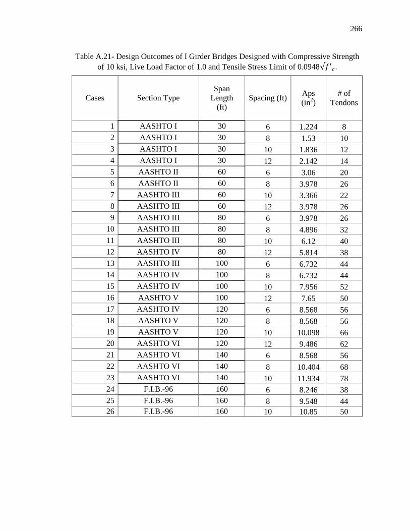
266
Table A.21- Design Outcomes of I Girder Bridges Designed with Compressive Strength
of 10 ksi, Live Load Factor of 1.0 and Tensile Stress Limit of 0.0948 .
Cases Section Type
Span
Length
(ft)
Spacing (ft) Aps
(in2)
# of
Tendons
1 AASHTO I 30 6 1.224 8
2 AASHTO I 30 8 1.53 10
3 AASHTO I 30 10 1.836 12
4 AASHTO I 30 12 2.142 14
5 AASHTO II 60 6 3.06 20
6 AASHTO II 60 8 3.978 26
7 AASHTO III 60 10 3.366 22
8 AASHTO III 60 12 3.978 26
9 AASHTO III 80 6 3.978 26
10 AASHTO III 80 8 4.896 32
11 AASHTO III 80 10 6.12 40
12 AASHTO IV 80 12 5.814 38
13 AASHTO III 100 6 6.732 44
14 AASHTO IV 100 8 6.732 44
15 AASHTO IV 100 10 7.956 52
16 AASHTO V 100 12 7.65 50
17 AASHTO IV 120 6 8.568 56
18 AASHTO V 120 8 8.568 56
19 AASHTO V 120 10 10.098 66
20 AASHTO VI 120 12 9.486 62
21 AASHTO VI 140 6 8.568 56
22 AASHTO VI 140 8 10.404 68
23 AASHTO VI 140 10 11.934 78
24 F.I.B.-96 160 6 8.246 38
25 F.I.B.-96 160 8 9.548 44
26 F.I.B.-96 160 10 10.85 50

267
Table A.22- Design Outcomes of I Girder Bridges Designed with Compressive Strength
of 10 ksi, Live Load Factor of 1.0 and Tensile Stress Limit of 0.158 .
Cases Section Type
Span
Length
(ft)
Spacing (ft) Aps
(in2)
# of
Tendons
1 AASHTO I 30 6 1.224 8
2 AASHTO I 30 8 1.53 10
3 AASHTO I 30 10 1.53 10
4 AASHTO I 30 12 2.142 14
5 AASHTO II 60 6 2.754 18
6 AASHTO II 60 8 3.672 24
7 AASHTO III 60 10 3.06 20
8 AASHTO III 60 12 3.672 24
9 AASHTO III 80 6 3.672 24
10 AASHTO III 80 8 4.59 30
11 AASHTO III 80 10 5.508 36
12 AASHTO IV 80 12 5.202 34
13 AASHTO III 100 6 6.426 42
14 AASHTO IV 100 8 6.426 42
15 AASHTO IV 100 10 7.65 50
16 AASHTO V 100 12 7.038 46
17 AASHTO IV 120 6 7.956 52
18 AASHTO V 120 8 7.956 52
19 AASHTO V 120 10 9.18 60
20 AASHTO VI 120 12 8.874 58
21 AASHTO VI 140 6 7.956 52
22 AASHTO VI 140 8 9.486 62
23 AASHTO VI 140 10 11.322 74
24 F.I.B.-96 160 6 7.812 36
25 F.I.B.-96 160 8 9.114 42
26 F.I.B.-96 160 10 10.416 48

268
Table A.23- Design Outcomes of I Girder Bridges Designed with Compressive Strength
of 10 ksi, Live Load Factor of 1.0 and Tensile Stress Limit of 0.19 .
Cases Section Type
Span
Length
(ft)
Spacing (ft) Aps
(in2)
# of
Tendons
1 AASHTO I 30 6 1.224 8
2 AASHTO I 30 8 1.53 10
3 AASHTO I 30 10 1.53 10
4 AASHTO I 30 12 1.836 12
5 AASHTO II 60 6 2.448 16
6 AASHTO II 60 8 3.366 22
7 AASHTO III 60 10 2.754 18
8 AASHTO III 60 12 3.672 24
9 AASHTO III 80 6 3.672 24
10 AASHTO III 80 8 4.59 30
11 AASHTO III 80 10 5.508 36
12 AASHTO IV 80 12 5.202 34
13 AASHTO III 100 6 6.12 40
14 AASHTO IV 100 8 6.12 40
15 AASHTO IV 100 10 7.344 48
16 AASHTO V 100 12 6.732 44
17 AASHTO IV 120 6 7.65 50
18 AASHTO V 120 8 7.65 50
19 AASHTO V 120 10 8.874 58
20 AASHTO VI 120 12 8.568 56
21 AASHTO VI 140 6 7.65 50
22 AASHTO VI 140 8 9.18 60
23 AASHTO VI 140 10 11.016 72
24 F.I.B.-96 160 6 7.378 34
25 F.I.B.-96 160 8 8.68 40
26 F.I.B.-96 160 10 9.982 46

269
Table A.24- Design Outcomes of I Girder Bridges Designed with Compressive Strength
of 10 ksi, Live Load Factor of 1.0 and Tensile Stress Limit of 0.253 .
Cases Section Type
Span
Length
(ft)
Spacing (ft) Aps
(in2)
# of
Tendons
1 AASHTO I 30 6 1.224 8
2 AASHTO I 30 8 1.53 10
3 AASHTO I 30 10 1.53 10
4 AASHTO I 30 12 1.836 12
5 AASHTO II 60 6 2.448 16
6 AASHTO II 60 8 3.06 20
7 AASHTO III 60 10 2.754 18
8 AASHTO III 60 12 3.366 22
9 AASHTO III 80 6 3.366 22
10 AASHTO III 80 8 4.284 28
11 AASHTO III 80 10 5.202 34
12 AASHTO IV 80 12 4.59 30
13 AASHTO III 100 6 5.814 38
14 AASHTO IV 100 8 5.814 38
15 AASHTO IV 100 10 6.732 44
16 AASHTO V 100 12 6.426 42
17 AASHTO IV 120 6 7.344 48
18 AASHTO V 120 8 7.038 46
19 AASHTO V 120 10 8.262 54
20 AASHTO VI 120 12 8.262 54
21 AASHTO VI 140 6 7.038 46
22 AASHTO VI 140 8 8.874 58
23 AASHTO VI 140 10 10.404 68
24 F.I.B.-96 160 6 6.51 30
25 F.I.B.-96 160 8 8.246 38
26 F.I.B.-96 160 10 9.114 42
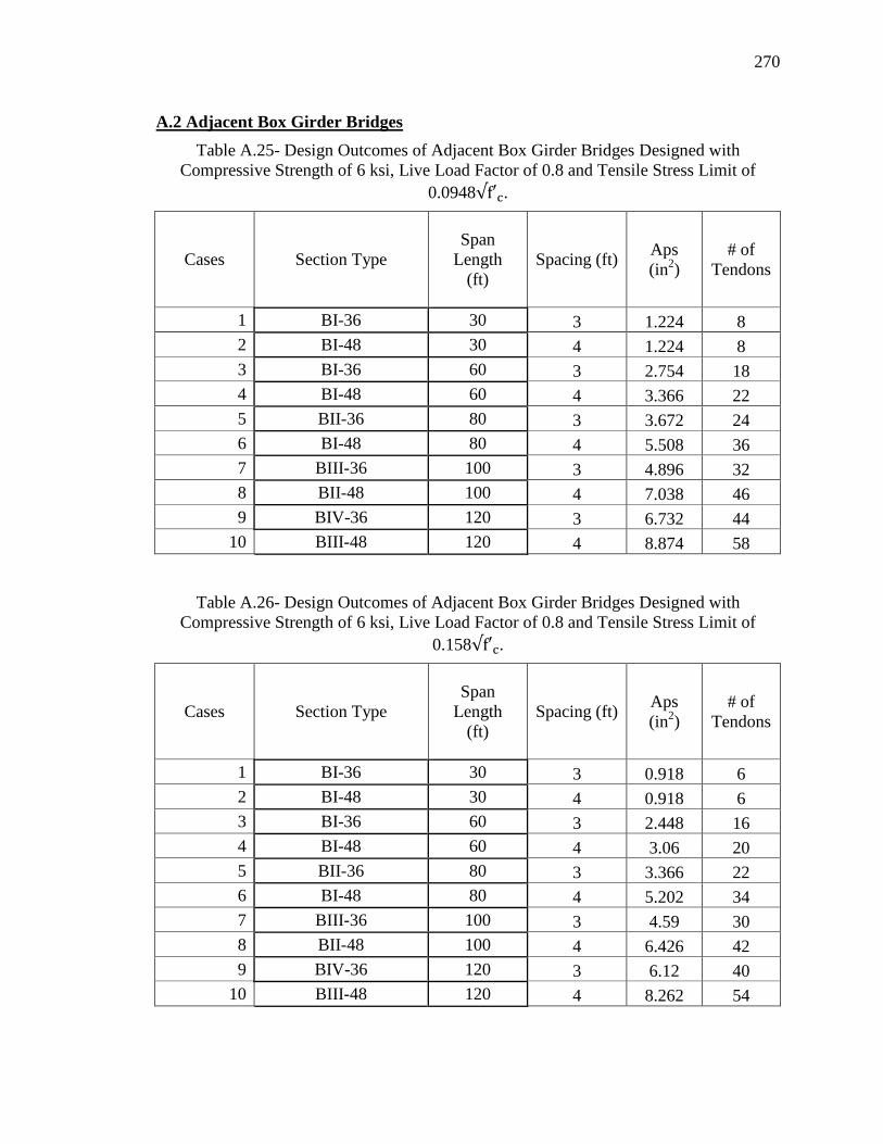
270
A.2 Adjacent Box Girder Bridges
Table A.25- Design Outcomes of Adjacent Box Girder Bridges Designed with
Compressive Strength of 6 ksi, Live Load Factor of 0.8 and Tensile Stress Limit of
0.0948 .
Cases Section Type
Span
Length
(ft)
Spacing (ft) Aps
(in2)
# of
Tendons
1 BI-36 30 3 1.224 8
2 BI-48 30 4 1.224 8
3 BI-36 60 3 2.754 18
4 BI-48 60 4 3.366 22
5 BII-36 80 3 3.672 24
6 BI-48 80 4 5.508 36
7 BIII-36 100 3 4.896 32
8 BII-48 100 4 7.038 46
9 BIV-36 120 3 6.732 44
10 BIII-48 120 4 8.874 58
Table A.26- Design Outcomes of Adjacent Box Girder Bridges Designed with
Compressive Strength of 6 ksi, Live Load Factor of 0.8 and Tensile Stress Limit of
0.158 .
Cases Section Type
Span
Length
(ft)
Spacing (ft) Aps
(in2)
# of
Tendons
1 BI-36 30 3 0.918 6
2 BI-48 30 4 0.918 6
3 BI-36 60 3 2.448 16
4 BI-48 60 4 3.06 20
5 BII-36 80 3 3.366 22
6 BI-48 80 4 5.202 34
7 BIII-36 100 3 4.59 30
8 BII-48 100 4 6.426 42
9 BIV-36 120 3 6.12 40
10 BIII-48 120 4 8.262 54

271
Table A.27- Design Outcomes of Adjacent Box Girder Bridges Designed with
Compressive Strength of 6 ksi, Live Load Factor of 0.8 and Tensile Stress Limit of
0.19 .
Cases Section Type
Span
Length
(ft)
Spacing (ft) Aps
(in2)
# of
Tendons
1 BI-36 30 3 0.918 6
2 BI-48 30 4 0.918 6
3 BI-36 60 3 2.448 16
4 BI-48 60 4 2.754 18
5 BII-36 80 3 3.366 22
6 BI-48 80 4 5.508 36
7 BIII-36 100 3 4.284 28
8 BII-48 100 4 6.426 42
9 BIV-36 120 3 6.12 40
10 BIII-48 120 4 7.956 52
Table A.28- Design Outcomes of Adjacent Box Girder Bridges Designed with
Compressive Strength of 6 ksi, Live Load Factor of 0.8 and Tensile Stress Limit of
0.253 .
Cases Section Type
Span
Length
(ft)
Spacing (ft) Aps
(in2)
# of
Tendons
1 BI-36 30 3 0.612 4
2 BI-48 30 4 0.612 4
3 BI-36 60 3 2.142 14
4 BI-48 60 4 2.754 18
5 BII-36 80 3 3.06 20
6 BI-48 80 4 4.896 32
7 BIII-36 100 3 3.978 26
8 BII-48 100 4 6.12 40
9 BIV-36 120 3 5.814 38
10 BIII-48 120 4 7.344 48
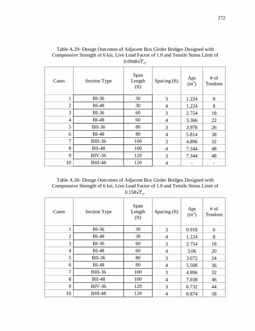
272
Table A.29- Design Outcomes of Adjacent Box Girder Bridges Designed with
Compressive Strength of 6 ksi, Live Load Factor of 1.0 and Tensile Stress Limit of
0.0948 .
Cases Section Type
Span
Length
(ft)
Spacing (ft) Aps
(in2)
# of
Tendons
1 BI-36 30 3 1.224 8
2 BI-48 30 4 1.224 8
3 BI-36 60 3 2.754 18
4 BI-48 60 4 3.366 22
5 BII-36 80 3 3.978 26
6 BI-48 80 4 5.814 38
7 BIII-36 100 3 4.896 32
8 BII-48 100 4 7.344 48
9 BIV-36 120 3 7.344 48
10 BIII-48 120 4 - -
Table A.30- Design Outcomes of Adjacent Box Girder Bridges Designed with
Compressive Strength of 6 ksi, Live Load Factor of 1.0 and Tensile Stress Limit of
0.158 .
Cases Section Type
Span
Length
(ft)
Spacing (ft) Aps
(in2)
# of
Tendons
1 BI-36 30 3 0.918 6
2 BI-48 30 4 1.224 8
3 BI-36 60 3 2.754 18
4 BI-48 60 4 3.06 20
5 BII-36 80 3 3.672 24
6 BI-48 80 4 5.508 36
7 BIII-36 100 3 4.896 32
8 BII-48 100 4 7.038 46
9 BIV-36 120 3 6.732 44
10 BIII-48 120 4 8.874 58

273
Table A.31- Design Outcomes of Adjacent Box Girder Bridges Designed with
Compressive Strength of 6 ksi, Live Load Factor of 1.0 and Tensile Stress Limit of
0.19 .
Cases Section Type
Span
Length
(ft)
Spacing (ft) Aps
(in2)
# of
Tendons
1 BI-36 30 3 0.918 6
2 BI-48 30 4 0.918 6
3 BI-36 60 3 2.448 16
4 BI-48 60 4 3.06 20
5 BII-36 80 3 3.366 22
6 BI-48 80 4 5.508 36
7 BIII-36 100 3 4.59 30
8 BII-48 100 4 6.732 44
9 BIV-36 120 3 6.426 42
10 BIII-48 120 4 8.568 56
Table A.32- Design Outcomes of Adjacent Box Girder Bridges Designed with
Compressive Strength of 6 ksi, Live Load Factor of 1.0 and Tensile Stress Limit of
0.253 .
Cases Section Type
Span
Length
(ft)
Spacing (ft) Aps
(in2)
# of
Tendons
1 BI-36 30 3 0.918 6
2 BI-48 30 4 0.612 4
3 BI-36 60 3 2.448 16
4 BI-48 60 4 2.754 18
5 BII-36 80 3 3.366 22
6 BI-48 80 4 5.202 34
7 BIII-36 100 3 4.284 28
8 BII-48 100 4 6.426 42
9 BIV-36 120 3 6.12 40
10 BIII-48 120 4 7.956 52

274
Table A.33- Design Outcomes of Adjacent Box Girder Bridges Designed with
Compressive Strength of 8 ksi, Live Load Factor of 0.8 and Tensile Stress Limit of
0.0948 .
Cases Section Type
Span
Length
(ft)
Spacing (ft) Aps
(in2)
# of
Tendons
1 BI-36 30 3 1.224 8
2 BI-48 30 4 1.224 8
3 BI-36 60 3 2.754 18
4 BI-48 60 4 3.06 20
5 BII-36 80 3 3.672 24
6 BI-48 80 4 5.202 34
7 BIII-36 100 3 4.59 30
8 BII-48 100 4 6.732 44
9 BIV-36 120 3 6.426 42
10 BIII-48 120 4 8.262 54
Table A.34- Design Outcomes of Adjacent Box Girder Bridges Designed with
Compressive Strength of 8 ksi, Live Load Factor of 0.8 and Tensile Stress Limit of
0.158 .
Cases Section Type
Span
Length
(ft)
Spacing (ft) Aps
(in2)
# of
Tendons
1 BI-36 30 3 0.918 6
2 BI-48 30 4 0.918 6
3 BI-36 60 3 2.448 16
4 BI-48 60 4 2.754 18
5 BII-36 80 3 3.366 22
6 BI-48 80 4 4.896 32
7 BIII-36 100 3 4.284 28
8 BII-48 100 4 6.12 40
9 BIV-36 120 3 5.814 38
10 BIII-48 120 4 7.65 50

275
Table A.35- Design Outcomes of Adjacent Box Girder Bridges Designed with
Compressive Strength of 8 ksi, Live Load Factor of 0.8 and Tensile Stress Limit of
0.19 .
Cases Section Type
Span
Length
(ft)
Spacing (ft) Aps
(in2)
# of
Tendons
1 BI-36 30 3 0.918 6
2 BI-48 30 4 0.918 6
3 BI-36 60 3 2.448 16
4 BI-48 60 4 2.754 18
5 BII-36 80 3 3.06 20
6 BI-48 80 4 4.896 32
7 BIII-36 100 3 4.284 28
8 BII-48 100 4 6.12 40
9 BIV-36 120 3 5.814 38
10 BIII-48 120 4 7.344 48
Table A.36- Design Outcomes of Adjacent Box Girder Bridges Designed with
Compressive Strength of 8 ksi, Live Load Factor of 0.8 and Tensile Stress Limit of
0.253 .
Cases Section Type
Span
Length
(ft)
Spacing (ft) Aps
(in2)
# of
Tendons
1 BI-36 30 3 0.612 4
2 BI-48 30 4 0.612 4
3 BI-36 60 3 2.142 14
4 BI-48 60 4 2.448 16
5 BII-36 80 3 3.06 20
6 BI-48 80 4 4.59 30
7 BIII-36 100 3 3.978 26
8 BII-48 100 4 5.814 38
9 BIV-36 120 3 5.508 36
10 BIII-48 120 4 7.038 46
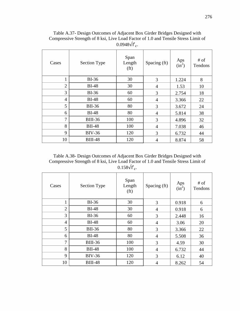
276
Table A.37- Design Outcomes of Adjacent Box Girder Bridges Designed with
Compressive Strength of 8 ksi, Live Load Factor of 1.0 and Tensile Stress Limit of
0.0948 .
Cases Section Type
Span
Length
(ft)
Spacing (ft) Aps
(in2)
# of
Tendons
1 BI-36 30 3 1.224 8
2 BI-48 30 4 1.53 10
3 BI-36 60 3 2.754 18
4 BI-48 60 4 3.366 22
5 BII-36 80 3 3.672 24
6 BI-48 80 4 5.814 38
7 BIII-36 100 3 4.896 32
8 BII-48 100 4 7.038 46
9 BIV-36 120 3 6.732 44
10 BIII-48 120 4 8.874 58
Table A.38- Design Outcomes of Adjacent Box Girder Bridges Designed with
Compressive Strength of 8 ksi, Live Load Factor of 1.0 and Tensile Stress Limit of
0.158 .
Cases Section Type
Span
Length
(ft)
Spacing (ft) Aps
(in2)
# of
Tendons
1 BI-36 30 3 0.918 6
2 BI-48 30 4 0.918 6
3 BI-36 60 3 2.448 16
4 BI-48 60 4 3.06 20
5 BII-36 80 3 3.366 22
6 BI-48 80 4 5.508 36
7 BIII-36 100 3 4.59 30
8 BII-48 100 4 6.732 44
9 BIV-36 120 3 6.12 40
10 BIII-48 120 4 8.262 54

277
Table A.39- Design Outcomes of Adjacent Box Girder Bridges Designed with
Compressive Strength of 8 ksi, Live Load Factor of 1.0 and Tensile Stress Limit of
0.19 .
Cases Section Type
Span
Length
(ft)
Spacing (ft) Aps
(in2)
# of
Tendons
1 BI-36 30 3 0.918 6
2 BI-48 30 4 0.918 6
3 BI-36 60 3 2.448 16
4 BI-48 60 4 3.06 20
5 BII-36 80 3 3.366 22
6 BI-48 80 4 5.202 34
7 BIII-36 100 3 4.284 28
8 BII-48 100 4 6.426 42
9 BIV-36 120 3 6.12 40
10 BIII-48 120 4 7.956 52
Table A.40- Design Outcomes of Adjacent Box Girder Bridges Designed with
Compressive Strength of 8 ksi, Live Load Factor of 1.0 and Tensile Stress Limit of
0.253 .
Cases Section Type
Span
Length
(ft)
Spacing (ft) Aps
(in2)
# of
Tendons
1 BI-36 30 3 0.612 4
2 BI-48 30 4 0.612 4
3 BI-36 60 3 2.142 14
4 BI-48 60 4 2.754 18
5 BII-36 80 3 3.06 20
6 BI-48 80 4 4.896 32
7 BIII-36 100 3 3.978 26
8 BII-48 100 4 6.12 40
9 BIV-36 120 3 5.814 38
10 BIII-48 120 4 7.344 48

278
A.3 Spread Box Girder Bridges
Table A.41- Design Outcomes of Spread Box Girder Bridges Designed with Compressive
Strength of 6ksi, Live Load Factor of 0.8 and Tensile Stress Limit of 0.0948 .
Cases Section Type Span Length (ft) Spacing (ft) Aps (in2) # of Tendons
1 BI-36 30 6 1.53 10
2 BI-36 30 8 1.836 12
3 BI-36 30 10 1.836 12
4 BI-36 30 12 2.142 14
5 BI-36 60 6 4.284 28
6 BI-36 60 8 4.896 32
7 BI-36 60 10 4.59 30
8 BI-48 60 12 5.202 34
9 BI-48 80 6 5.814 38
10 BII-48 80 8 5.814 38
11 BII-48 80 10 6.426 42
12 BIII-48 80 12 7.038 46
13 BIII-48 100 6 7.344 48
14 BIII-48 100 8 - -
15 BIV-48 100 10 - -
Table A.42- Design Outcomes of Spread Box Girder Bridges Designed with Compressive
Strength of 6ksi, Live Load Factor of 0.8 and Tensile Stress Limit of 0.158 .
Cases Section Type Span Length (ft) Spacing (ft) Aps (in2) # of Tendons
1 BI-36 30 6 1.224 8
2 BI-36 30 8 1.53 10
3 BI-36 30 10 1.836 12
4 BI-36 30 12 1.836 12
5 BI-36 60 6 3.978 26
6 BI-36 60 8 4.896 32
7 BI-36 60 10 4.284 28
8 BI-48 60 12 4.896 32
9 BI-48 80 6 5.508 36
10 BII-48 80 8 5.508 36
11 BII-48 80 10 6.12 40
12 BIII-48 80 12 6.426 42
13 BIII-48 100 6 7.038 46
14 BIII-48 100 8 - -
15 BIV-48 100 10 - -

279
Table A.43- Design Outcomes of Spread Box Girder Bridges Designed with Compressive
Strength of 6ksi, Live Load Factor of 0.8 and Tensile Stress Limit of 0.19 .
Cases Section Type Span Length (ft) Spacing (ft) Aps (in2) # of Tendons
1 BI-36 30 6 1.224 8
2 BI-36 30 8 1.53 10
3 BI-36 30 10 1.53 10
4 BI-36 30 12 1.836 12
5 BI-36 60 6 3.672 24
6 BI-36 60 8 4.59 30
7 BI-36 60 10 3.978 26
8 BI-48 60 12 4.59 30
9 BI-48 80 6 5.202 34
10 BII-48 80 8 5.202 34
11 BII-48 80 10 6.12 40
12 BIII-48 80 12 6.426 42
13 BIII-48 100 6 7.038 46
14 BIII-48 100 8 - -
15 BIV-48 100 10 - -
Table A.44- Design Outcomes of Spread Box Girder Bridges Designed with Compressive
Strength of 6ksi, Live Load Factor of 0.8 and Tensile Stress Limit of 0.253 .
Cases Section Type Span Length (ft) Spacing (ft) Aps (in2) # of Tendons
1 BI-36 30 6 1.224 8
2 BI-36 30 8 1.224 8
3 BI-36 30 10 1.53 10
4 BI-36 30 12 1.53 10
5 BI-36 60 6 3.672 24
6 BI-36 60 8 4.284 28
7 BII-36 60 10 3.978 26
8 BII-48 60 12 4.284 28
9 BII-48 80 6 4.896 32
10 BIII-48 80 8 4.896 32
11 BIII-48 80 10 5.814 38
12 BIV-48 80 12 5.814 38
13 BIII-48 100 6 6.426 42
14 BIII-48 100 8 - -
15 BIV-48 100 10 - -
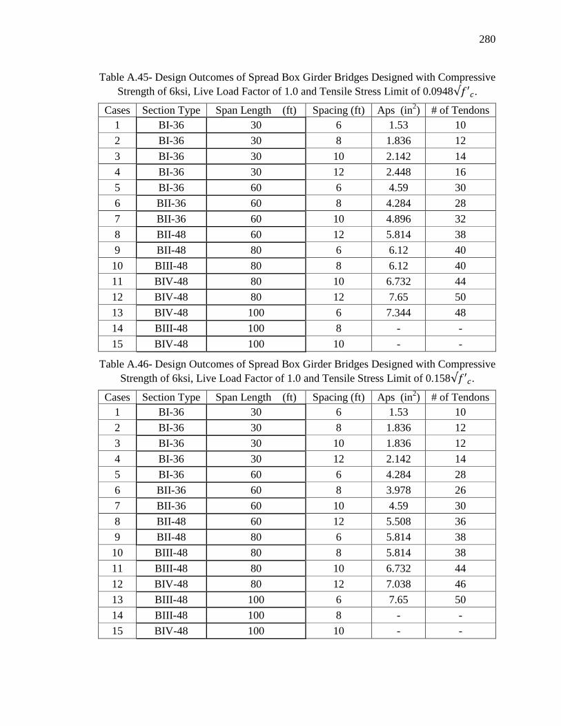
280
Table A.45- Design Outcomes of Spread Box Girder Bridges Designed with Compressive
Strength of 6ksi, Live Load Factor of 1.0 and Tensile Stress Limit of 0.0948 .
Cases Section Type Span Length (ft) Spacing (ft) Aps (in2) # of Tendons
1 BI-36 30 6 1.53 10
2 BI-36 30 8 1.836 12
3 BI-36 30 10 2.142 14
4 BI-36 30 12 2.448 16
5 BI-36 60 6 4.59 30
6 BII-36 60 8 4.284 28
7 BII-36 60 10 4.896 32
8 BII-48 60 12 5.814 38
9 BII-48 80 6 6.12 40
10 BIII-48 80 8 6.12 40
11 BIV-48 80 10 6.732 44
12 BIV-48 80 12 7.65 50
13 BIV-48 100 6 7.344 48
14 BIII-48 100 8 - -
15 BIV-48 100 10 - -
Table A.46- Design Outcomes of Spread Box Girder Bridges Designed with Compressive
Strength of 6ksi, Live Load Factor of 1.0 and Tensile Stress Limit of 0.158 .
Cases Section Type Span Length (ft) Spacing (ft) Aps (in2) # of Tendons
1 BI-36 30 6 1.53 10
2 BI-36 30 8 1.836 12
3 BI-36 30 10 1.836 12
4 BI-36 30 12 2.142 14
5 BI-36 60 6 4.284 28
6 BII-36 60 8 3.978 26
7 BII-36 60 10 4.59 30
8 BII-48 60 12 5.508 36
9 BII-48 80 6 5.814 38
10 BIII-48 80 8 5.814 38
11 BIII-48 80 10 6.732 44
12 BIV-48 80 12 7.038 46
13 BIII-48 100 6 7.65 50
14 BIII-48 100 8 - -
15 BIV-48 100 10 - -
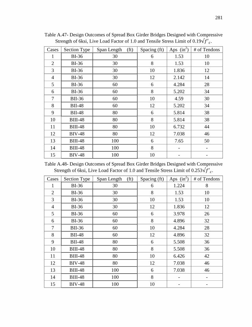
281
Table A.47- Design Outcomes of Spread Box Girder Bridges Designed with Compressive
Strength of 6ksi, Live Load Factor of 1.0 and Tensile Stress Limit of 0.19 .
Cases Section Type Span Length (ft) Spacing (ft) Aps (in2) # of Tendons
1 BI-36 30 6 1.53 10
2 BI-36 30 8 1.53 10
3 BI-36 30 10 1.836 12
4 BI-36 30 12 2.142 14
5 BI-36 60 6 4.284 28
6 BI-36 60 8 5.202 34
7 BII-36 60 10 4.59 30
8 BII-48 60 12 5.202 34
9 BII-48 80 6 5.814 38
10 BIII-48 80 8 5.814 38
11 BIII-48 80 10 6.732 44
12 BIV-48 80 12 7.038 46
13 BIII-48 100 6 7.65 50
14 BIII-48 100 8 - -
15 BIV-48 100 10 - -
Table A.48- Design Outcomes of Spread Box Girder Bridges Designed with Compressive
Strength of 6ksi, Live Load Factor of 1.0 and Tensile Stress Limit of 0.253 .
Cases Section Type Span Length (ft) Spacing (ft) Aps (in2) # of Tendons
1 BI-36 30 6 1.224 8
2 BI-36 30 8 1.53 10
3 BI-36 30 10 1.53 10
4 BI-36 30 12 1.836 12
5 BI-36 60 6 3.978 26
6 BI-36 60 8 4.896 32
7 BII-36 60 10 4.284 28
8 BII-48 60 12 4.896 32
9 BII-48 80 6 5.508 36
10 BIII-48 80 8 5.508 36
11 BIII-48 80 10 6.426 42
12 BIV-48 80 12 7.038 46
13 BIII-48 100 6 7.038 46
14 BIII-48 100 8 - -
15 BIV-48 100 10 - -

282
Table A.49- Design Outcomes of Spread Box Girder Bridges Designed with Compressive
Strength of 8ksi, Live Load Factor of 0.8 and Tensile Stress Limit of 0.0948 .
Cases Section Type Span Length
(ft) Spacing (ft) Aps (in
2) # of Tendons
1 BI-36 30 6 1.53 10
2 BI-36 30 8 1.836 12
3 BI-36 30 10 1.836 12
4 BI-36 30 12 2.142 14
5 BI-36 60 6 3.978 26
6 BI-36 60 8 4.896 32
7 BI-36 60 10 5.508 36
8 BI-48 60 12 6.426 42
9 BI-48 80 6 7.038 46
10 BII-48 80 8 6.732 44
11 BII-48 80 10 7.65 50
12 BIII-48 80 12 7.038 46
13 BIII-48 100 6 7.344 48
14 BIII-48 100 8 9.18 60
15 BIV-48 100 10 10.404 68
Table A.50- Design Outcomes of Spread Box Girder Bridges Designed with Compressive
Strength of 8ksi, Live Load Factor of 0.8 and Tensile Stress Limit of 0.158 .
Cases Section Type Span Length (ft) Spacing (ft) Aps (in2) # of Tendons
1 BI-36 30 6 1.224 8
2 BI-36 30 8 1.53 10
3 BI-36 30 10 1.836 12
4 BI-36 30 12 1.836 12
5 BI-36 60 6 3.672 24
6 BI-36 60 8 4.59 30
7 BI-36 60 10 5.202 34
8 BI-48 60 12 5.814 38
9 BI-48 80 6 6.732 44
10 BII-48 80 8 6.12 40
11 BII-48 80 10 7.344 48
12 BIII-48 80 12 6.732 44
13 BIII-48 100 6 7.038 46
14 BIII-48 100 8 8.262 54
15 BIV-48 100 10 9.18 60

283
Table A.51- Design Outcomes of Spread Box Girder Bridges Designed with Compressive
Strength of 8ksi, Live Load Factor of 0.8 and Tensile Stress Limit of 0.19 .
Cases Section Type Span Length (ft) Spacing (ft) Aps (in2)
# of
Tendons
1 BI-36 30 6 1.224 8
2 BI-36 30 8 1.53 10
3 BI-36 30 10 1.53 10
4 BI-36 30 12 1.836 12
5 BI-36 60 6 3.672 24
6 BI-36 60 8 4.284 28
7 BI-36 60 10 5.202 34
8 BI-48 60 12 5.814 38
9 BI-48 80 6 6.426 42
10 BII-48 80 8 6.12 40
11 BII-48 80 10 7.038 46
12 BIII-48 80 12 6.732 44
13 BIII-48 100 6 6.732 44
14 BIII-48 100 8 7.956 52
15 BIV-48 100 10 8.568 56
Table A.52- Design Outcomes of Spread Box Girder Bridges Designed with Compressive
Strength of 8ksi, Live Load Factor of 0.8 and Tensile Stress Limit of 0.253 .
Cases Section Type Span Length (ft) Spacing (ft) Aps (in2) # of Tendons
1 BI-36 30 6 0.918 6
2 BI-36 30 8 1.224 8
3 BI-36 30 10 1.53 10
4 BI-36 30 12 1.53 10
5 BI-36 60 6 3.366 22
6 BI-36 60 8 4.284 28
7 BI-36 60 10 4.896 32
8 BI-48 60 12 5.508 36
9 BI-48 80 6 6.12 40
10 BII-48 80 8 5.814 38
11 BII-48 80 10 6.732 44
12 BIII-48 80 12 6.12 40
13 BIII-48 100 6 6.426 42
14 BIII-48 100 8 7.65 50
15 BIV-48 100 10 7.956 52
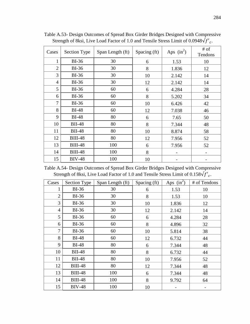
284
Table A.53- Design Outcomes of Spread Box Girder Bridges Designed with Compressive
Strength of 8ksi, Live Load Factor of 1.0 and Tensile Stress Limit of 0.0948 .
Cases Section Type Span Length (ft) Spacing (ft) Aps (in2)
# of
Tendons
1 BI-36 30 6 1.53 10
2 BI-36 30 8 1.836 12
3 BI-36 30 10 2.142 14
4 BI-36 30 12 2.142 14
5 BI-36 60 6 4.284 28
6 BI-36 60 8 5.202 34
7 BI-36 60 10 6.426 42
8 BI-48 60 12 7.038 46
9 BI-48 80 6 7.65 50
10 BII-48 80 8 7.344 48
11 BII-48 80 10 8.874 58
12 BIII-48 80 12 7.956 52
13 BIII-48 100 6 7.956 52
14 BIII-48 100 8 - -
15 BIV-48 100 10 - -
Table A.54- Design Outcomes of Spread Box Girder Bridges Designed with Compressive
Strength of 8ksi, Live Load Factor of 1.0 and Tensile Stress Limit of 0.158 .
Cases Section Type Span Length (ft) Spacing (ft) Aps (in2) # of Tendons
1 BI-36 30 6 1.53 10
2 BI-36 30 8 1.53 10
3 BI-36 30 10 1.836 12
4 BI-36 30 12 2.142 14
5 BI-36 60 6 4.284 28
6 BI-36 60 8 4.896 32
7 BI-36 60 10 5.814 38
8 BI-48 60 12 6.732 44
9 BI-48 80 6 7.344 48
10 BII-48 80 8 6.732 44
11 BII-48 80 10 7.956 52
12 BIII-48 80 12 7.344 48
13 BIII-48 100 6 7.344 48
14 BIII-48 100 8 9.792 64
15 BIV-48 100 10 - -

285
Table A.55- Design Outcomes of Spread Box Girder Bridges Designed with Compressive
Strength of 8ksi, Live Load Factor of 1.0 and Tensile Stress Limit of 0.19 .
Cases Section Type Span Length (ft) Spacing (ft) Aps (in2)
# of
Tendons
1 BI-36 30 6 1.224 8
2 BI-36 30 8 1.53 10
3 BI-36 30 10 1.836 12
4 BI-36 30 12 1.836 12
5 BI-36 60 6 3.978 26
6 BI-36 60 8 4.896 32
7 BI-36 60 10 5.814 38
8 BI-48 60 12 6.426 42
9 BI-48 80 6 7.038 46
10 BII-48 80 8 6.732 44
11 BII-48 80 10 7.956 52
12 BIII-48 80 12 7.344 48
13 BIII-48 100 6 7.038 46
14 BIII-48 100 8 9.18 60
15 BIV-48 100 10 - -
Table A.56- Design Outcomes of Spread Box Girder Bridges Designed with Compressive
Strength of 8ksi, Live Load Factor of 1.0 and Tensile Stress Limit of 0.253 .
Cases Section Type Span Length (ft) Spacing (ft) Aps (in2)
# of
Tendons
1 BI-36 30 6 1.224 8
2 BI-36 30 8 1.224 8
3 BI-36 30 10 1.53 10
4 BI-36 30 12 1.836 12
5 BI-36 60 6 3.672 24
6 BI-36 60 8 4.59 30
7 BI-36 60 10 5.508 36
8 BI-48 60 12 6.12 40
9 BI-48 80 6 6.732 44
10 BII-48 80 8 6.426 42
11 BII-48 80 10 7.344 48
12 BIII-48 80 12 6.732 44
13 BIII-48 100 6 6.732 44
14 BIII-48 100 8 8.568 56
15 BIV-48 100 10 8.874 58

286
Table A.57- Design Outcomes of Spread Box Girder Bridges Designed with Compressive
Strength of 10ksi, Live Load Factor of 0.8 and Tensile Stress Limit of 0.0948 .
Cases Section Type Span Length (ft) Spacing (ft) Aps (in2)
# of
Tendons
1 BI-36 30 6 1.53 10
2 BI-36 30 8 1.53 10
3 BI-36 30 10 1.836 12
4 BI-36 30 12 2.142 14
5 BI-36 60 6 3.978 26
6 BI-36 60 8 4.59 30
7 BI-36 60 10 5.508 36
8 BI-48 60 12 6.12 40
9 BI-48 80 6 6.732 44
10 BII-48 80 8 6.426 42
11 BII-48 80 10 7.344 48
12 BIII-48 80 12 7.038 46
13 BIII-48 100 6 7.038 46
14 BIII-48 100 8 8.568 56
15 BIV-48 100 10 9.486 62
Table A.58- Design Outcomes of Spread Box Girder Bridges Designed with Compressive
Strength of 10ksi, Live Load Factor of 0.8 and Tensile Stress Limit of 0.158 .
Cases Section Type Span Length (ft) Spacing (ft) Aps (in2)
# of
Tendons
1 BI-36 30 6 1.224 8
2 BI-36 30 8 1.53 10
3 BI-36 30 10 1.53 10
4 BI-36 30 12 1.836 12
5 BI-36 60 6 3.672 24
6 BI-36 60 8 4.284 28
7 BI-36 60 10 5.202 34
8 BI-48 60 12 5.814 38
9 BI-48 80 6 6.426 42
10 BII-48 80 8 6.12 40
11 BII-48 80 10 7.038 46
12 BIII-48 80 12 6.426 42
13 BIII-48 100 6 6.732 44
14 BIII-48 100 8 7.956 52
15 BIV-48 100 10 8.568 56

287
Table A.59- Design Outcomes of Spread Box Girder Bridges Designed with Compressive
Strength of 10ksi, Live Load Factor of 0.8 and Tensile Stress Limit of 0.19 .
Cases Section Type Span Length (ft) Spacing (ft) Aps (in2)
# of
Tendons
1 BI-36 30 6 1.224 8
2 BI-36 30 8 1.224 8
3 BI-36 30 10 1.53 10
4 BI-36 30 12 1.836 12
5 BI-36 60 6 3.672 24
6 BI-36 60 8 4.284 28
7 BI-36 60 10 4.896 32
8 BI-48 60 12 5.508 36
9 BI-48 80 6 6.426 42
10 BII-48 80 8 5.814 38
11 BII-48 80 10 6.732 44
12 BIII-48 80 12 6.426 42
13 BIII-48 100 6 6.732 44
14 BIII-48 100 8 7.65 50
15 BIV-48 100 10 8.262 54
Table A.60- Design Outcomes of Spread Box Girder Bridges Designed with Compressive
Strength of 10ksi, Live Load Factor of 0.8 and Tensile Stress Limit of 0.253 .
Cases Section Type Span Length (ft) Spacing (ft) Aps (in2)
# of
Tendons
1 BI-36 30 6 0.918 6
2 BI-36 30 8 1.224 8
3 BI-36 30 10 1.224 8
4 BI-36 30 12 1.53 10
5 BI-36 60 6 3.366 22
6 BI-36 60 8 3.978 26
7 BI-36 60 10 4.59 30
8 BI-48 60 12 5.202 34
9 BI-48 80 6 5.814 38
10 BII-48 80 8 5.508 36
11 BII-48 80 10 6.426 42
12 BIII-48 80 12 5.814 38
13 BIII-48 100 6 6.12 40
14 BIII-48 100 8 7.344 48
15 BIV-48 100 10 7.65 50

288
Table A.61- Design Outcomes of Spread Box Girder Bridges Designed with Compressive
Strength of 10ksi, Live Load Factor of 1.0 and Tensile Stress Limit of 0.0948 .
Cases Section Type Span Length (ft) Spacing (ft) Aps (in2)
# of
Tendons
1 BI-36 30 6 1.53 10
2 BI-36 30 8 1.836 12
3 BI-36 30 10 2.142 14
4 BI-36 30 12 2.142 14
5 BI-36 60 6 4.284 28
6 BI-36 60 8 5.202 34
7 BI-36 60 10 6.12 40
8 BI-48 60 12 6.732 44
9 BI-48 80 6 7.344 48
10 BII-48 80 8 7.038 46
11 BII-48 80 10 8.262 54
12 BIII-48 80 12 7.65 50
13 BIII-48 100 6 7.65 50
14 BIII-48 100 8 - -
15 BIV-48 100 10 - -
Table A.62- Design Outcomes of Spread Box Girder Bridges Designed with Compressive
Strength of 10ksi, Live Load Factor of 1.0 and Tensile Stress Limit of 0.158 .
Cases Section Type Span Length (ft) Spacing (ft) Aps (in2)
# of
Tendons
1 BI-36 30 6 1.53 10
2 BI-36 30 8 1.53 10
3 BI-36 30 10 1.836 12
4 BI-36 30 12 2.142 14
5 BI-36 60 6 3.978 26
6 BI-36 60 8 4.896 32
7 BI-36 60 10 5.814 38
8 BI-48 60 12 6.426 42
9 BI-48 80 6 7.038 46
10 BII-48 80 8 6.732 44
11 BII-48 80 10 7.65 50
12 BIII-48 80 12 7.344 48
13 BIII-48 100 6 7.344 48
14 BIII-48 100 8 8.874 58
15 BIV-48 100 10 10.098 66
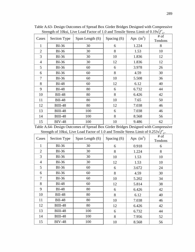
289
Table A.63- Design Outcomes of Spread Box Girder Bridges Designed with Compressive
Strength of 10ksi, Live Load Factor of 1.0 and Tensile Stress Limit of 0.19 .
Cases Section Type Span Length (ft) Spacing (ft) Aps (in2)
# of
Tendons
1 BI-36 30 6 1.224 8
2 BI-36 30 8 1.53 10
3 BI-36 30 10 1.836 12
4 BI-36 30 12 1.836 12
5 BI-36 60 6 3.978 26
6 BI-36 60 8 4.59 30
7 BI-36 60 10 5.508 36
8 BI-48 60 12 6.12 40
9 BI-48 80 6 6.732 44
10 BII-48 80 8 6.426 42
11 BII-48 80 10 7.65 50
12 BIII-48 80 12 7.038 46
13 BIII-48 100 6 7.038 46
14 BIII-48 100 8 8.568 56
15 BIV-48 100 10 9.486 62
Table A.64- Design Outcomes of Spread Box Girder Bridges Designed with Compressive
Strength of 10ksi, Live Load Factor of 1.0 and Tensile Stress Limit of 0.253 .
Cases Section Type Span Length (ft) Spacing (ft) Aps (in2)
# of
Tendons
1 BI-36 30 6 0.918 6
2 BI-36 30 8 1.224 8
3 BI-36 30 10 1.53 10
4 BI-36 30 12 1.53 10
5 BI-36 60 6 3.672 24
6 BI-36 60 8 4.59 30
7 BI-36 60 10 5.202 34
8 BI-48 60 12 5.814 38
9 BI-48 80 6 6.426 42
10 BII-48 80 8 6.12 40
11 BII-48 80 10 7.038 46
12 BIII-48 80 12 6.426 42
13 BIII-48 100 6 6.732 44
14 BIII-48 100 8 7.956 52
15 BIV-48 100 10 8.568 56

290
A.4 PCI ASBI Box Girder Bridge
Table A.65- Design Outcomes of Spread Box Girder Bridges Designed with Compressive
Strength of 8ksi, Live Load Factor of 0.8 and Tensile Stress Limit of 0.0948 .
Cases Section Type Span Length (ft) Aps (in2)
# of
Tendons
1 1800-2 100 7.344 48
2 1800-2 120 10.71 70
3 1800-2 140 14.076 92
4 2100-2 160 21.266 98
5 2400-2 180 22.568 104
6 2400-2 200 27.342 126
Table A.66- Design Outcomes of Spread Box Girder Bridges Designed with Compressive
Strength of 8ksi, Live Load Factor of 0.8 and Tensile Stress Limit of 0.158 .
Cases Section Type Span Length (ft) Aps (in2)
# of
Tendons
1 1800-2 100 5.814 38
2 1800-2 120 9.18 60
3 1800-2 140 12.546 82
4 2100-2 160 19.096 88
5 2400-2 180 20.398 94
6 2400-2 200 25.172 116
Table A.67- Design Outcomes of Spread Box Girder Bridges Designed with Compressive
Strength of 8ksi, Live Load Factor of 0.8 and Tensile Stress Limit of 0.19 .
Cases Section Type Span Length (ft) Aps (in2)
# of
Tendons
1 1800-2 100 5.202 34
2 1800-2 120 8.568 56
3 1800-2 140 11.934 78
4 2100-2 160 17.794 82
5 2400-2 180 19.096 88
6 2400-2 200 24.304 112
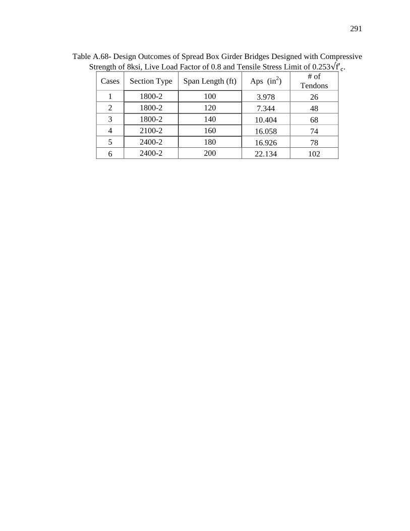
291
Table A.68- Design Outcomes of Spread Box Girder Bridges Designed with Compressive
Strength of 8ksi, Live Load Factor of 0.8 and Tensile Stress Limit of 0.253 .
Cases Section Type Span Length (ft) Aps (in2)
# of
Tendons
1 1800-2 100 3.978 26
2 1800-2 120 7.344 48
3 1800-2 140 10.404 68
4 2100-2 160 16.058 74
5 2400-2 180 16.926 78
6 2400-2 200 22.134 102

292
A.5 Existing Bridges from NCHRP 12-78
Table A.69- Summary of NCHRP 12-78 I-Girder Bridge
Bridge
Name Section Type
Girder
Spacing (ft.)
Span Length
(ft.)
Aps
(in2)
# of
Tendons
82 MN type 63 10.33 82.75 5.20 34
3107 36'' I BEAM 5.77 49.54 1.84 12
4794 BEAM Type 4 9.33 66.67 5.05 33
4827 BEAM Type 2 7.17 50.58 2.75 18
5624 BEAM Type 4 7.25 59.37 3.06 20
5794 BEAM Type 3 5.83 72.00 4.34 20
5840 BEAM Type 6 9.00 85.00 4.59 30
5884 BEAM Type 6 8.17 90.01 5.81 38
8330 BEAM Type 6 8.67 76.38 4.28 28
8783 AASHTO VI 7.75 143.15 9.98 46
8832 36'' I BEAM 10.00 43.26 3.06 20
8885 BT-63 10.58 90.01 5.51 36
8889 BT-63 10.58 90.85 5.51 36
8890 AASHTO VI 8.00 143.50 10.42 48
8891 BEAM Type 6 9.25 47.17 2.14 14
8957 BEAM Type 6 8.67 98.00 5.64 26
9378 Wisconsin
Girder 10.42 101.83 6.12 40
10269 AASHTO III 6.67 78.00 4.28 28
10599 AASHTO II 6.75 62.83 4.28 28
10740 AASHTO III 7.00 78.55 4.90 32
10755 AASHTO II 7.00 52.50 3.67 24
10803 BT-72 6.00 138.25 7.68 46
11030 BT-72 6.38 136.00 7.65 50
11938 BT-63 7.31 116.52 7.68 46
12589 AASHTO IV 8.75 73.21 4.59 30
12596 AASHTO IV 11.15 96.79 10.85 50
12603 AASHTO II 11.48 37.73 3.04 14
12610 AASHTO IV 7.13 108.53 7.96 52
15620 Bulb-Tee 5.35 119.82 10.42 48
18067 AL BT-54
Mod. 5.29 131.02 10.85 50

293
Table A.70- Summary of NCHRP 12-78 Spread Box Girder Bridge
Bridge
Name Section Type
Girder
Spacing (ft.)
Span Length
(ft.)
Aps
(in2)
# of
Tendons
1150 33" x 36" Box 8.50 70.58 5.97 39
3577 27"x36" IDOT 6.70 38.58 2.92 27
3754 33"x36" IDOT 6.36 53.61 3.24 30
8875 27"x48" P/S Box 11.25 38.00 3.52 23
9090 MDOT 33" Box 7.08 66.04 4.34 20
9091 MDOT 33" Box 7.08 66.20 4.34 20
9128 1525 Box 7.49 33.69 0.87 4
9192 21" x 36" Box 9.83 38.67 2.75 18
9217 17" Box 6.21 42.30 3.47 16
9219 MDOT 21" Box 5.25 53.17 3.47 16
9243 33in x 36in Box 6.17 73.33 4.56 21
9248 21 in Box Beam 8.00 37.75 3.91 18
9282 17" x 36" Box 7.83 36.30 2.45 16
9284 17" x 36" Box 6.66 31.56 1.95 9
9286 27" x 36" Box 8.04 50.67 4.34 20
9310 21" x 36" Box 5.97 51.97 4.34 20
9324 27" x 36" Box 10.50 42.33 3.06 20
9328 27" x 36" Box 6.92 57.27 3.98 26
9349 21" x 36" Box 7.00 48.67 3.37 22
9355 39" x 36" Box 7.92 75.20 5.64 26
9356 39" x 36" Box 7.92 75.20 5.64 26
9361 27" x 36" Box 6.00 65.79 4.59 30
9368 33" x 36" Box 7.38 71.25 4.59 30
9369 27" x 36" Box 6.50 51.32 3.04 14
9370 27" x 36" Box 6.42 51.32 3.04 14
9376 27" x 36" Box 7.38 53.35 3.26 15
9380 21" x 36" Box 9.10 32.09 1.84 12
9383 27" x 36" Box 10.58 46.82 3.47 16
9384 21" x 36" Box 6.60 44.13 3.04 14
9394 27x 48 in Box 7.50 66.91 5.20 34
12870 36" x 48" 6.50 77.50 4.59 30
14969 BIV-48 7.88 78.74 7.34 48
16293 1220 x 1220
box 8.86 57.27 5.64 26
16366 Beams B1-B6 6.58 60.38 5.81 38
17240 BII-48 8.00 51.50 3.67 24
17338 BII-48 8.00 49.00 2.75 18
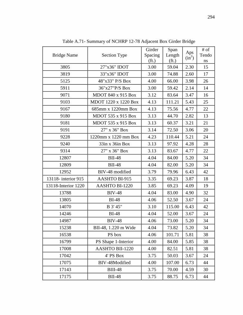
294
Table A.71- Summary of NCHRP 12-78 Adjacent Box Girder Bridge
Bridge Name Section Type
Girder
Spacing
(ft.)
Span
Length
(ft.)
Aps
(in2)
# of
Tendo
ns
3805 27"x36" IDOT 3.00 59.04 2.30 15
3819 33"x36" IDOT 3.00 74.88 2.60 17
5125 48"x33" P/S Box 4.00 66.00 3.98 26
5911 36"x27"P/S Box 3.00 59.42 2.14 14
9071 MDOT 840 x 915 Box 3.12 83.64 3.47 16
9103 MDOT 1220 x 1220 Box 4.13 111.21 5.43 25
9167 685mm x 1220mm Box 4.13 75.56 4.77 22
9180 MDOT 535 x 915 Box 3.13 44.70 2.82 13
9181 MDOT 535 x 915 Box 3.13 60.37 3.21 21
9191 27" x 36" Box 3.14 72.50 3.06 20
9228 1220mm x 1220 mm Box 4.23 110.44 5.21 24
9240 33in x 36in Box 3.13 97.92 4.28 28
9314 27" x 36" Box 3.13 83.67 4.77 22
12807 BII-48 4.04 84.00 5.20 34
12809 BII-48 4.04 82.00 5.20 34
12952 BIV-48 modified 3.79 79.96 6.43 42
13118- interior 915 AASHTO BI-915 3.35 69.23 3.87 18
13118-Interior 1220 AASHTO BI-1220 3.85 69.23 4.09 19
13788 BIV-48 4.04 83.00 4.90 32
13805 BI-48 4.06 52.50 3.67 24
14070 B 3' 45" 3.10 115.00 6.43 42
14246 BI-48 4.04 52.00 3.67 24
14987 BIV-48 4.06 73.00 5.20 34
15238 BII-48, 1.220 m Wide 4.04 73.82 5.20 34
16538 PS box 4.06 101.71 5.81 38
16799 PS Shape 1-Interior 4.00 84.00 5.85 38
17008 AASHTO BII-1220 4.00 82.51 5.81 38
17042 4' PS Box 3.75 50.03 3.67 24
17075 BIV-48Modified 4.00 107.00 6.73 44
17143 BIII-48 3.75 70.00 4.59 30
17175 BII-48 3.75 88.75 6.73 44

295
APPENDIX B. RELIABILITY ANALYSIS RESULTS
APPENDIX B
RELIABILITY ANALYSIS RESULTS
This appendix contains reliability analysis results for prestressed concrete girders
designed using various girder types for various design criteria considering different
traffic volume.
B.1 I Girder Bridges
Figure B.1 Reliability Indices for AASHTO I Girder Bridges at Decompression Limit
State (ADTT=1000), γLL=0.8 ( 0.0948t cf f )

296
Figure B.2 Reliability Indices for AASHTO I Girder Bridges at Maximum Allowable
Tensile Stress Limit State (ADTT=1000), γLL=0.8 ( 0.0948t cf f )
Figure B.3 Reliability Indices for AASHTO I Girder Bridges at Maximum Allowable
Crack Width Limit State (ADTT=1000), γLL=0.8 ( 0.0948t cf f )

297
Figure B.4 Reliability Indices for AASHTO I Girder Bridges at Decompression Limit
State (ADTT=1000), γLL=1.0 ( 0.0948t cf f )
Figure B.5 Reliability Indices for AASHTO I Girder Bridges at Maximum Tensile Stress
Limit State (ADTT=1000), γLL=1.0 ( 0.0948t cf f )
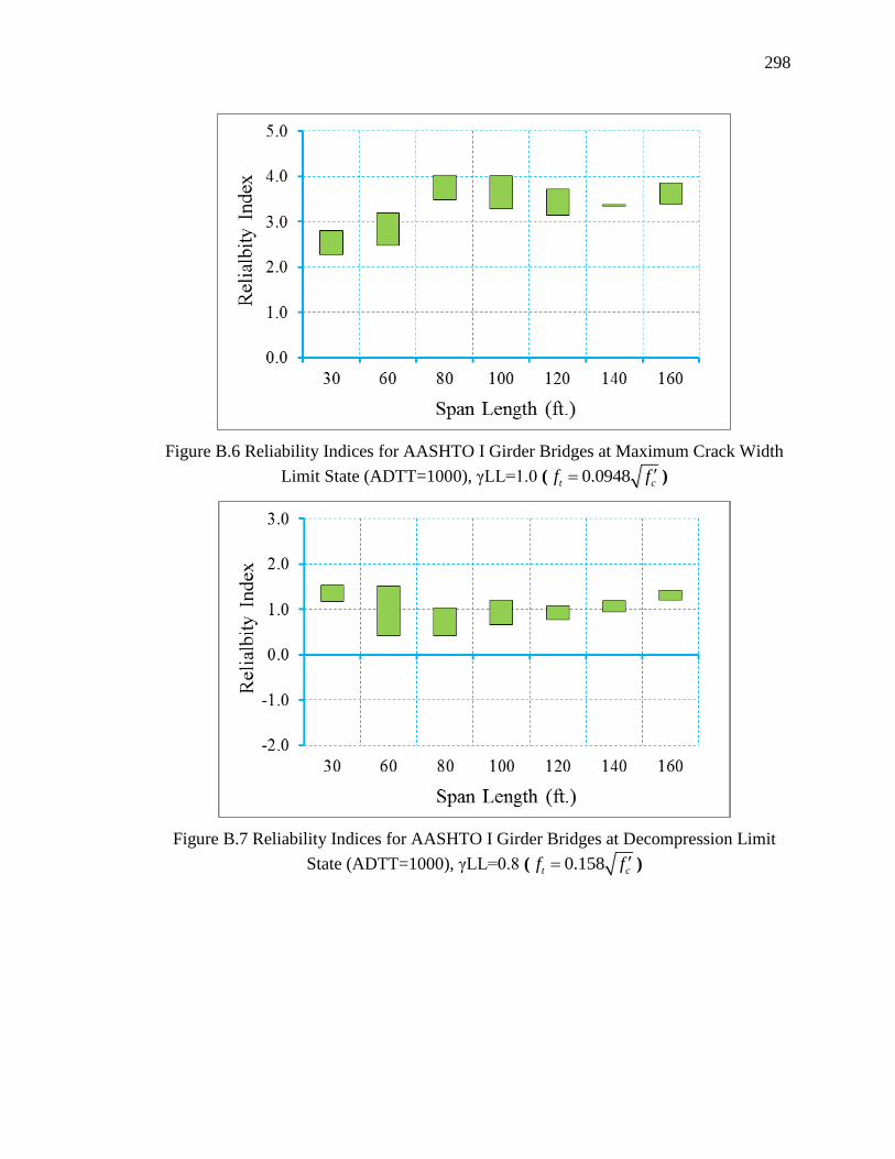
298
Figure B.6 Reliability Indices for AASHTO I Girder Bridges at Maximum Crack Width
Limit State (ADTT=1000), γLL=1.0 ( 0.0948t cf f )
Figure B.7 Reliability Indices for AASHTO I Girder Bridges at Decompression Limit
State (ADTT=1000), γLL=0.8 ( 0.158t cf f )
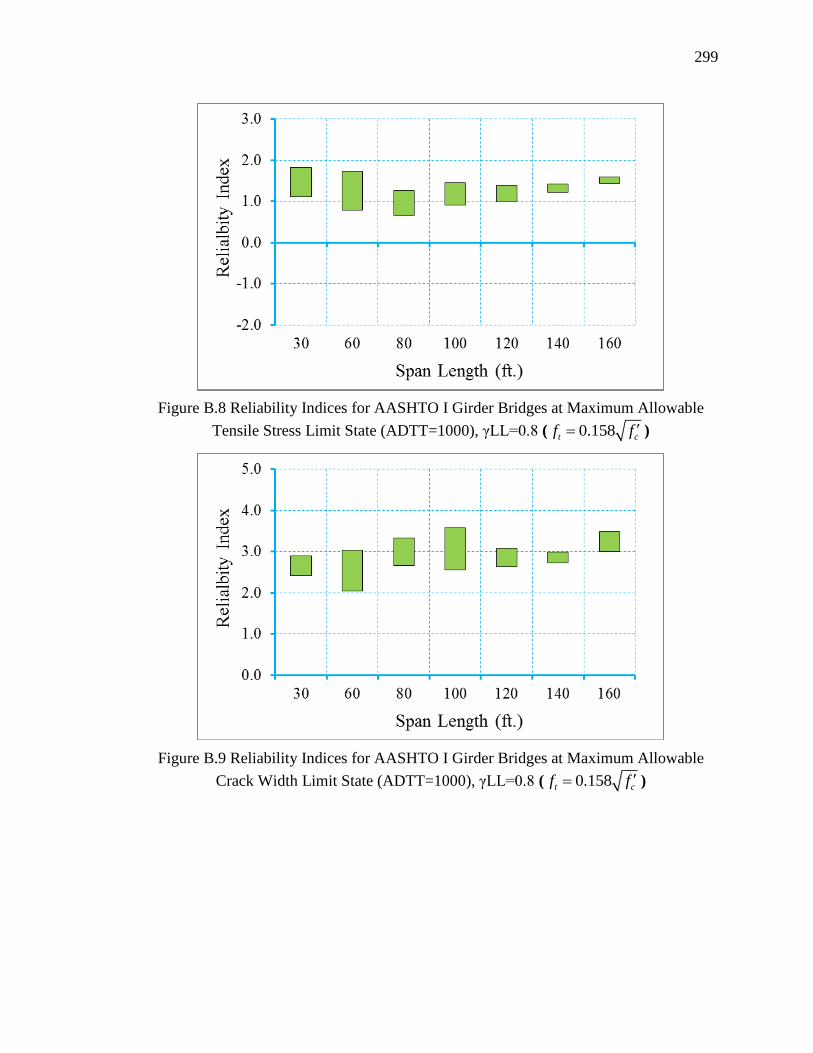
299
Figure B.8 Reliability Indices for AASHTO I Girder Bridges at Maximum Allowable
Tensile Stress Limit State (ADTT=1000), γLL=0.8 ( 0.158t cf f )
Figure B.9 Reliability Indices for AASHTO I Girder Bridges at Maximum Allowable
Crack Width Limit State (ADTT=1000), γLL=0.8 ( 0.158t cf f )
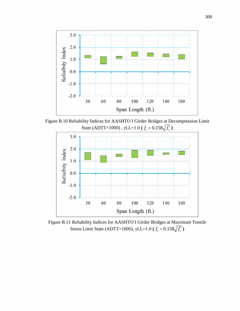
300
Figure B.10 Reliability Indices for AASHTO I Girder Bridges at Decompression Limit
State (ADTT=1000) , γLL=1.0 ( 0.158t cf f )
Figure B.11 Reliability Indices for AASHTO I Girder Bridges at Maximum Tensile
Stress Limit State (ADTT=1000), γLL=1.0 ( 0.158t cf f )

301
Figure B.12 Reliability Indices for AASHTO I Girder Bridges at Maximum Crack Width
Limit State (ADTT=1000), γLL=1.0 ( 0.158t cf f )
Figure B.13 Reliability Indices for AASHTO I Girder Bridges at Decompression Limit
State (ADTT=1000), γLL=0.8 ( 0.19t cf f )

302
Figure B.14 Reliability Indices for AASHTO I Girder Bridges at Maximum Allowable
Tensile Stress Limit State (ADTT=1000), γLL=0.8 ( 0.19t cf f )
Figure B.15 Reliability Indices for AASHTO I Girder Bridges at Maximum Allowable
Crack Width Limit State (ADTT=1000), γLL=0.8 ( 0.19t cf f )
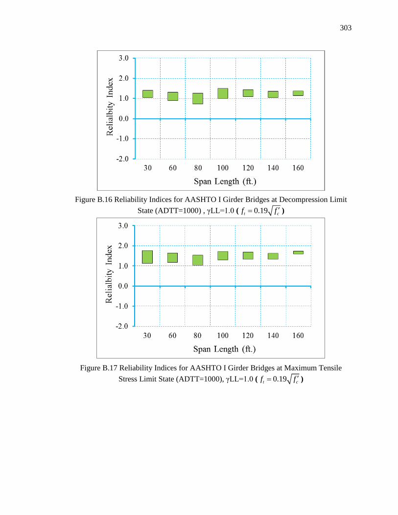
303
Figure B.16 Reliability Indices for AASHTO I Girder Bridges at Decompression Limit
State (ADTT=1000) , γLL=1.0 ( 0.19t cf f )
Figure B.17 Reliability Indices for AASHTO I Girder Bridges at Maximum Tensile
Stress Limit State (ADTT=1000), γLL=1.0 ( 0.19t cf f )

304
Figure B.18 Reliability Indices for AASHTO I Girder Bridges at Maximum Crack Width
Limit State (ADTT=1000), γLL=1.0 ( 0.19t cf f )
Figure B.19 Reliability Indices for AASHTO I Girder Bridges at Decompression Limit
State (ADTT=1000), γLL=0.8 ( 0.253t cf f )

305
Figure B.20 Reliability Indices for AASHTO I Girder Bridges at Maximum Allowable
Tensile Stress Limit State (ADTT=1000), γLL=0.8 ( 0.253t cf f )
Figure B.21 Reliability Indices for AASHTO I Girder Bridges at Maximum Allowable
Crack Width Limit State (ADTT=1000), γLL=0.8 ( 0.253t cf f )

306
Figure B.22 Reliability Indices for AASHTO I Girder Bridges at Decompression Limit
State (ADTT=1000), γLL=1.0 ( 0.253t cf f )
Figure B.23 Reliability Indices for AASHTO I Girder Bridges at Maximum Allowable
Tensile Stress Limit State (ADTT=1000), γLL=1.0 ( 0.253t cf f )
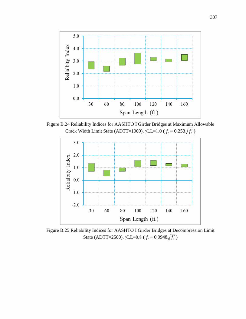
307
Figure B.24 Reliability Indices for AASHTO I Girder Bridges at Maximum Allowable
Crack Width Limit State (ADTT=1000), γLL=1.0 ( 0.253t cf f )
Figure B.25 Reliability Indices for AASHTO I Girder Bridges at Decompression Limit
State (ADTT=2500), γLL=0.8 ( 0.0948t cf f )
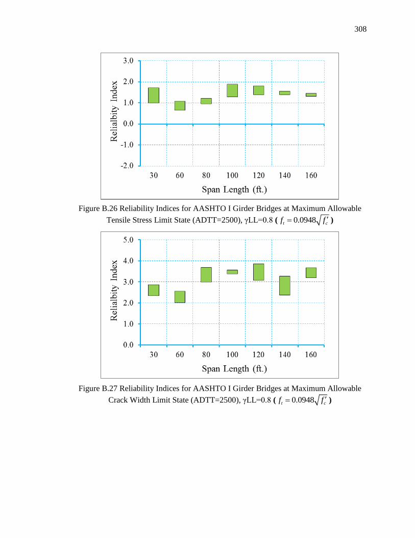
308
Figure B.26 Reliability Indices for AASHTO I Girder Bridges at Maximum Allowable
Tensile Stress Limit State (ADTT=2500), γLL=0.8 ( 0.0948t cf f )
Figure B.27 Reliability Indices for AASHTO I Girder Bridges at Maximum Allowable
Crack Width Limit State (ADTT=2500), γLL=0.8 ( 0.0948t cf f )

309
Figure B.28 Reliability Indices for AASHTO I Girder Bridges at Decompression Limit
State (ADTT=2500), γLL=1.0 ( 0.0948t cf f )
Figure B.29 Reliability Indices for AASHTO I Girder Bridges at Maximum Tensile
Stress Limit State (ADTT=2500), γLL=1.0 ( 0.0948t cf f )
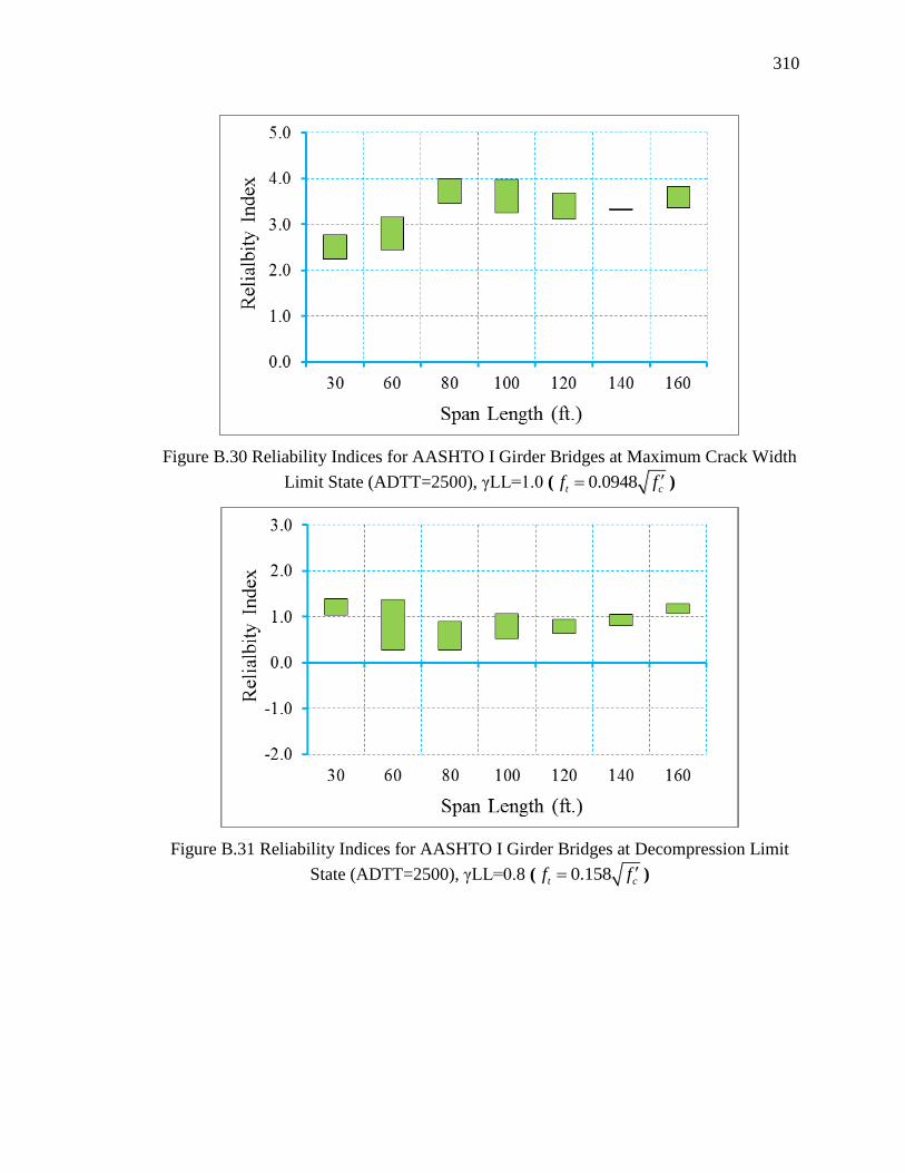
310
Figure B.30 Reliability Indices for AASHTO I Girder Bridges at Maximum Crack Width
Limit State (ADTT=2500), γLL=1.0 ( 0.0948t cf f )
Figure B.31 Reliability Indices for AASHTO I Girder Bridges at Decompression Limit
State (ADTT=2500), γLL=0.8 ( 0.158t cf f )

311
Figure B.32 Reliability Indices for AASHTO I Girder Bridges at Maximum Allowable
Tensile Stress Limit State (ADTT=2500), γLL=0.8 ( 0.158t cf f )
Figure B.33 Reliability Indices for AASHTO I Girder Bridges at Maximum Allowable
Crack Width Limit State (ADTT=2500), γLL=0.8 ( 0.158t cf f )
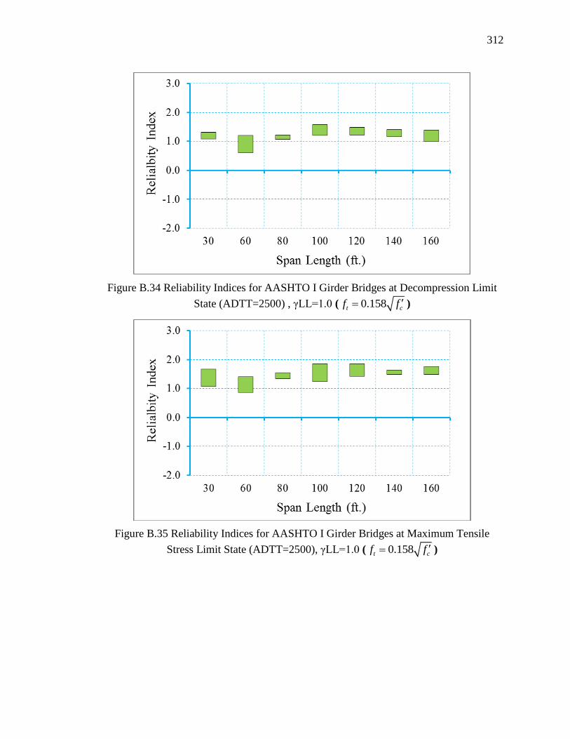
312
Figure B.34 Reliability Indices for AASHTO I Girder Bridges at Decompression Limit
State (ADTT=2500) , γLL=1.0 ( 0.158t cf f )
Figure B.35 Reliability Indices for AASHTO I Girder Bridges at Maximum Tensile
Stress Limit State (ADTT=2500), γLL=1.0 ( 0.158t cf f )
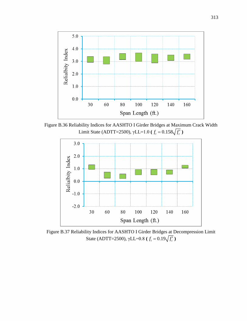
313
Figure B.36 Reliability Indices for AASHTO I Girder Bridges at Maximum Crack Width
Limit State (ADTT=2500), γLL=1.0 ( 0.158t cf f )
Figure B.37 Reliability Indices for AASHTO I Girder Bridges at Decompression Limit
State (ADTT=2500), γLL=0.8 ( 0.19t cf f )
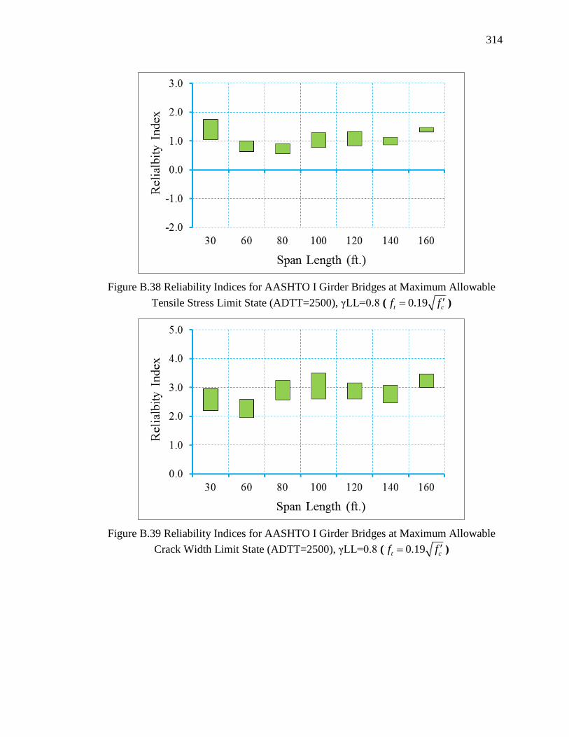
314
Figure B.38 Reliability Indices for AASHTO I Girder Bridges at Maximum Allowable
Tensile Stress Limit State (ADTT=2500), γLL=0.8 ( 0.19t cf f )
Figure B.39 Reliability Indices for AASHTO I Girder Bridges at Maximum Allowable
Crack Width Limit State (ADTT=2500), γLL=0.8 ( 0.19t cf f )
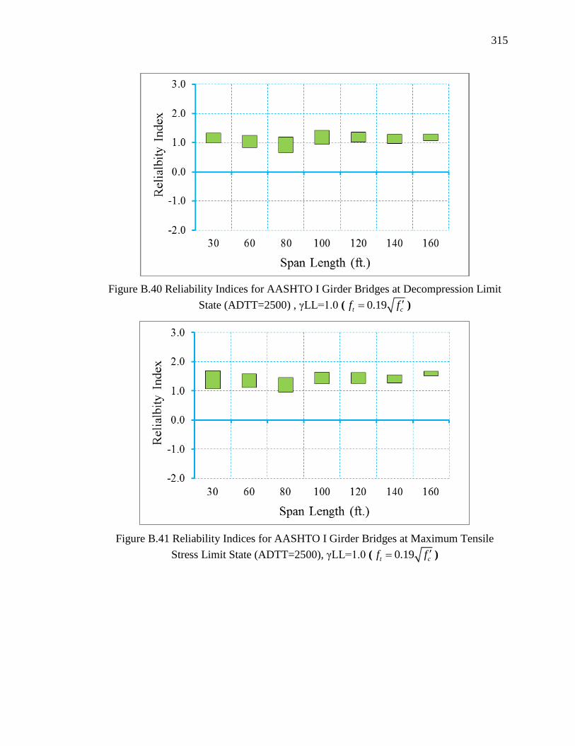
315
Figure B.40 Reliability Indices for AASHTO I Girder Bridges at Decompression Limit
State (ADTT=2500) , γLL=1.0 ( 0.19t cf f )
Figure B.41 Reliability Indices for AASHTO I Girder Bridges at Maximum Tensile
Stress Limit State (ADTT=2500), γLL=1.0 ( 0.19t cf f )

316
Figure B.42 Reliability Indices for AASHTO I Girder Bridges at Maximum Crack Width
Limit State (ADTT=2500), γLL=1.0 ( 0.19t cf f )
Figure B.43 Reliability Indices for AASHTO I Girder Bridges at Decompression Limit
State (ADTT=2500), γLL=0.8 ( 0.253t cf f )
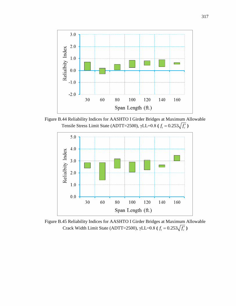
317
Figure B.44 Reliability Indices for AASHTO I Girder Bridges at Maximum Allowable
Tensile Stress Limit State (ADTT=2500), γLL=0.8 ( 0.253t cf f )
Figure B.45 Reliability Indices for AASHTO I Girder Bridges at Maximum Allowable
Crack Width Limit State (ADTT=2500), γLL=0.8 ( 0.253t cf f )

318
Figure B.46 Reliability Indices for AASHTO I Girder Bridges at Decompression Limit
State (ADTT=2500) , γLL=1.0 ( 0.253t cf f )
Figure B.47 Reliability Indices for AASHTO I Girder Bridges at Maximum Tensile
Stress Limit State (ADTT=2500), γLL=1.0 ( 0.253t cf f )
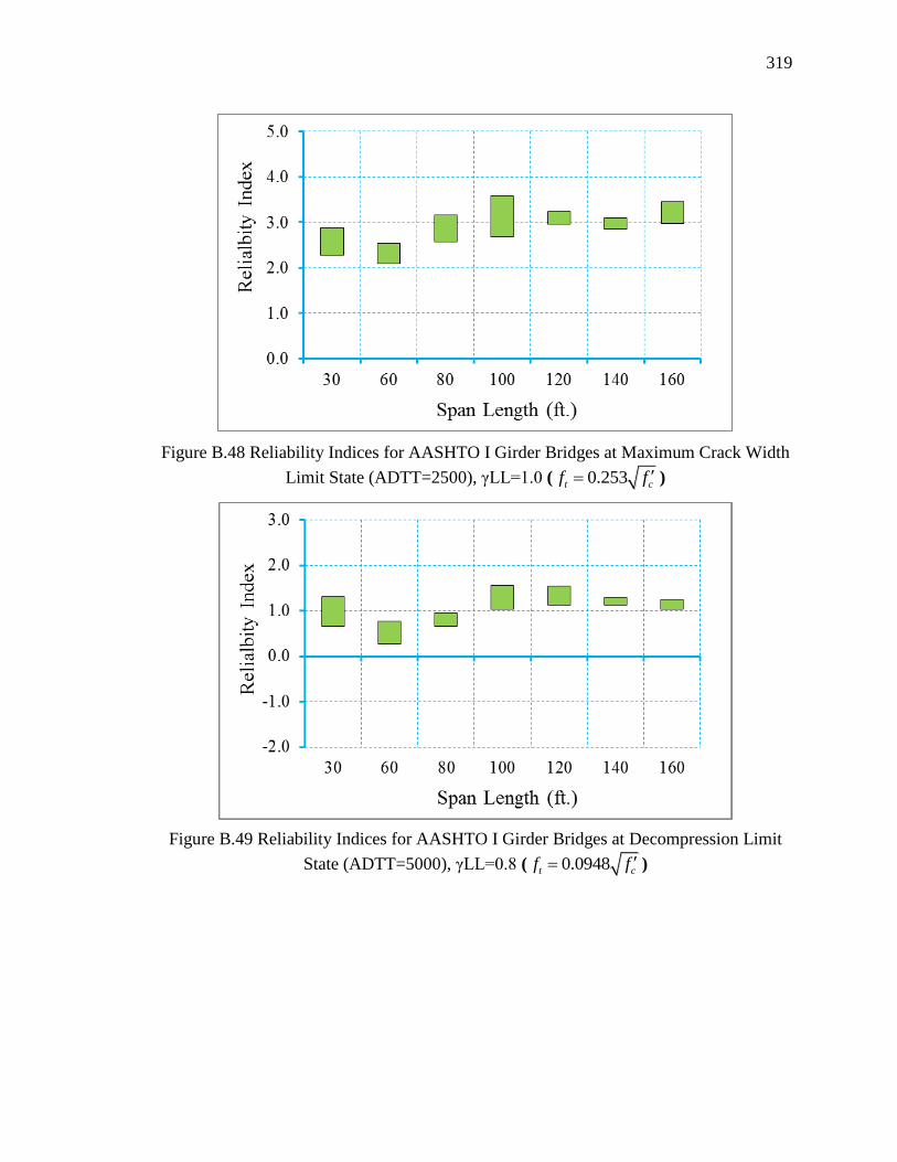
319
Figure B.48 Reliability Indices for AASHTO I Girder Bridges at Maximum Crack Width
Limit State (ADTT=2500), γLL=1.0 ( 0.253t cf f )
Figure B.49 Reliability Indices for AASHTO I Girder Bridges at Decompression Limit
State (ADTT=5000), γLL=0.8 ( 0.0948t cf f )

320
Figure B.50 Reliability Indices for AASHTO I Girder Bridges at Maximum Allowable
Tensile Stress Limit State (ADTT=5000), γLL=0.8 ( 0.0948t cf f )
Figure B.51 Reliability Indices for AASHTO I Girder Bridges at Maximum Allowable
Crack Width Limit State (ADTT=5000), γLL=0.8 ( 0.0948t cf f )

321
Figure B.52 Reliability Indices for AASHTO I Girder Bridges at Decompression Limit
State (ADTT=5000), γLL=1.0 ( 0.0948t cf f )
Figure B.53 Reliability Indices for AASHTO I Girder Bridges at Maximum Tensile
Stress Limit State (ADTT=5000), γLL=1.0 ( 0.0948t cf f )
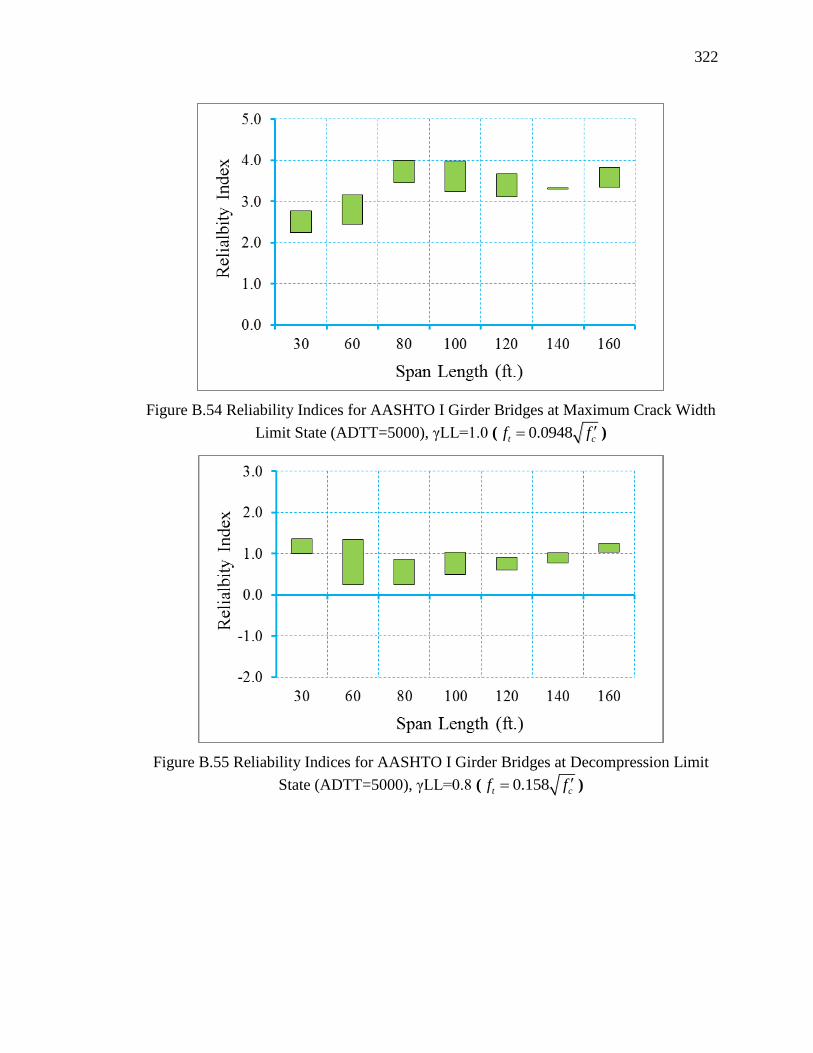
322
Figure B.54 Reliability Indices for AASHTO I Girder Bridges at Maximum Crack Width
Limit State (ADTT=5000), γLL=1.0 ( 0.0948t cf f )
Figure B.55 Reliability Indices for AASHTO I Girder Bridges at Decompression Limit
State (ADTT=5000), γLL=0.8 ( 0.158t cf f )

323
Figure B.56 Reliability Indices for AASHTO I Girder Bridges at Maximum Allowable
Tensile Stress Limit State (ADTT=5000), γLL=0.8 ( 0.158t cf f )
Figure B.57 Reliability Indices for AASHTO I Girder Bridges at Maximum Allowable
Crack Width Limit State (ADTT=5000), γLL=0.8 ( 0.158t cf f )

324
Figure B.58 Reliability Indices for AASHTO I Girder Bridges at Decompression Limit
State (ADTT=5000), γLL=1.0 ( 0.158t cf f )
Figure B.59 Reliability Indices for AASHTO I Girder Bridges at Maximum Tensile
Stress Limit State (ADTT=5000), γLL=1.0 ( 0.158t cf f )

325
Figure B.60 Reliability Indices for AASHTO I Girder Bridges at Maximum Crack Width
Limit State (ADTT=5000), γLL=1.0 ( 0.158t cf f )
Figure B.61 Reliability Indices for AASHTO I Girder Bridges at Decompression Limit
State (ADTT=5000), γLL=0.8 ( 0.19t cf f )
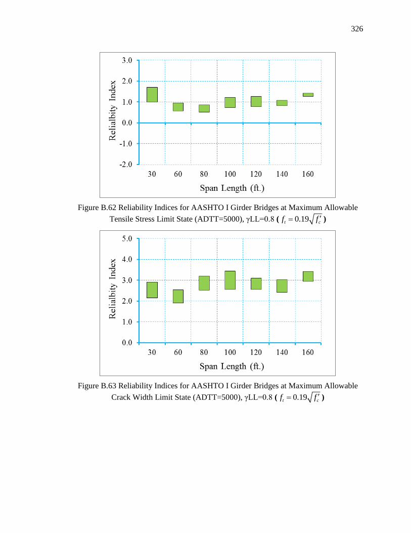
326
Figure B.62 Reliability Indices for AASHTO I Girder Bridges at Maximum Allowable
Tensile Stress Limit State (ADTT=5000), γLL=0.8 ( 0.19t cf f )
Figure B.63 Reliability Indices for AASHTO I Girder Bridges at Maximum Allowable
Crack Width Limit State (ADTT=5000), γLL=0.8 ( 0.19t cf f )
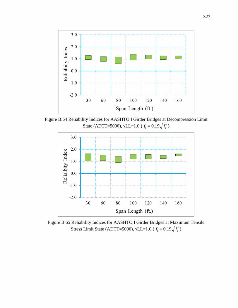
327
Figure B.64 Reliability Indices for AASHTO I Girder Bridges at Decompression Limit
State (ADTT=5000), γLL=1.0 ( 0.19t cf f )
Figure B.65 Reliability Indices for AASHTO I Girder Bridges at Maximum Tensile
Stress Limit State (ADTT=5000), γLL=1.0 ( 0.19t cf f )
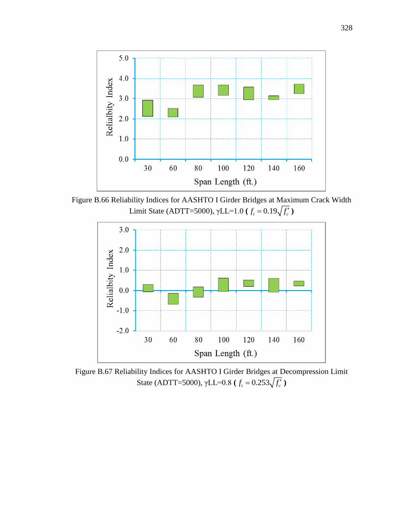
328
Figure B.66 Reliability Indices for AASHTO I Girder Bridges at Maximum Crack Width
Limit State (ADTT=5000), γLL=1.0 ( 0.19t cf f )
Figure B.67 Reliability Indices for AASHTO I Girder Bridges at Decompression Limit
State (ADTT=5000), γLL=0.8 ( 0.253t cf f )

329
Figure B.68 Reliability Indices for AASHTO I Girder Bridges at Maximum Allowable
Tensile Stress Limit State (ADTT=5000), γLL=0.8 ( 0.253t cf f )
Figure B.69 Reliability Indices for AASHTO I Girder Bridges at Maximum Allowable
Crack Width Limit State (ADTT=5000), γLL=0.8 ( 0.253t cf f )

330
Figure B.70 Reliability Indices for AASHTO I Girder Bridges at Decompression Limit
State (ADTT=5000), γLL=1.0 ( 0.253t cf f )
Figure B.71 Reliability Indices for AASHTO I Girder Bridges at Maximum Tensile
Stress Limit State (ADTT=5000), γLL=1.0 ( 0.253t cf f )

331
Figure B.72 Reliability Indices for AASHTO I Girder Bridges at Maximum Crack Width
Limit State (ADTT=5000), γLL=1.0 ( 0.253t cf f )
Figure B.73 Reliability Indices for AASHTO I Girder Bridges at Decompression Limit
State (ADTT=10000), γLL=0.8 ( 0.0948t cf f )
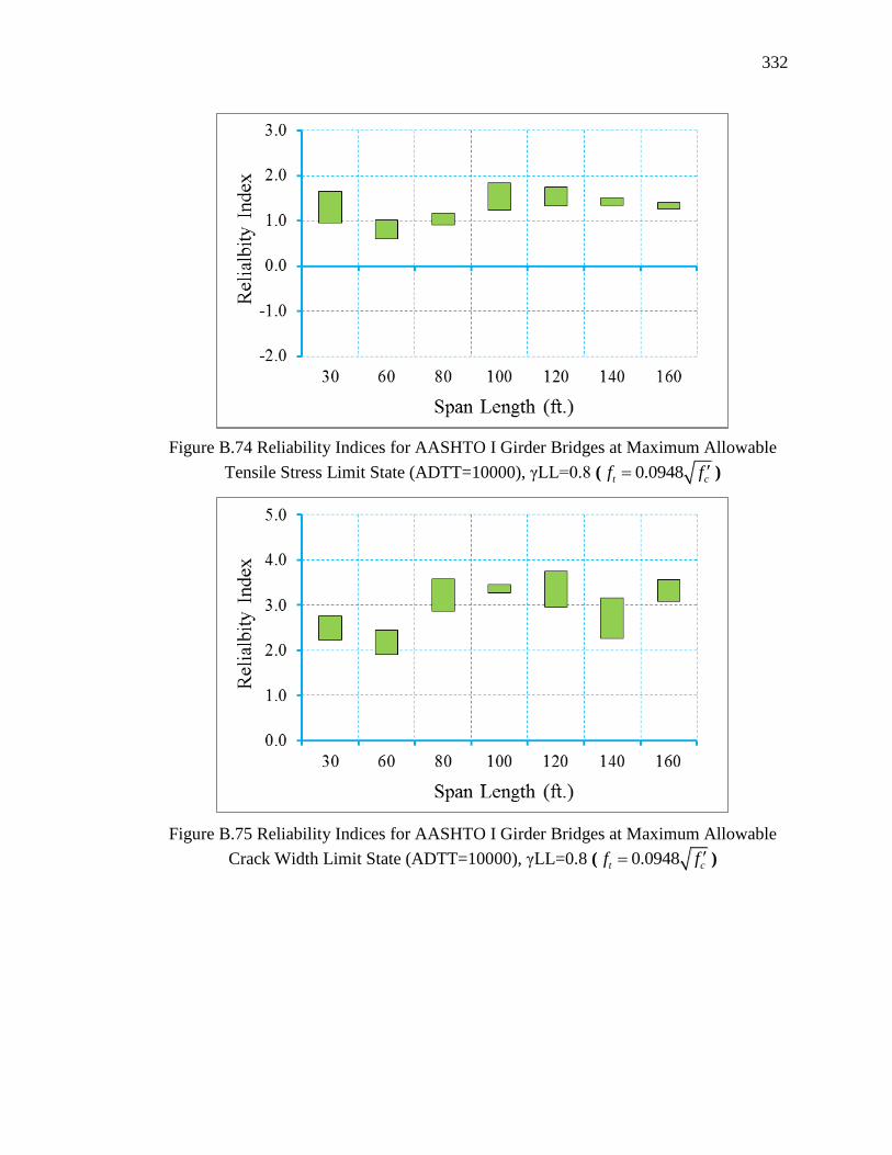
332
Figure B.74 Reliability Indices for AASHTO I Girder Bridges at Maximum Allowable
Tensile Stress Limit State (ADTT=10000), γLL=0.8 ( 0.0948t cf f )
Figure B.75 Reliability Indices for AASHTO I Girder Bridges at Maximum Allowable
Crack Width Limit State (ADTT=10000), γLL=0.8 ( 0.0948t cf f )

333
Figure B.76 Reliability Indices for AASHTO I Girder Bridges at Decompression Limit
State (ADTT=10000), γLL=1.0 ( 0.0948t cf f )
Figure B.77 Reliability Indices for AASHTO I Girder Bridges at Maximum Tensile
Stress Limit State (ADTT=10000), γLL=1.0 ( 0.0948t cf f )

334
Figure B.78 Reliability Indices for AASHTO I Girder Bridges at Maximum Crack Width
Limit State (ADTT=10000), γLL=1.0 ( 0.0948t cf f )
Figure B.79 Reliability Indices for AASHTO I Girder Bridges at Decompression Limit
State (ADTT=10000), γLL=0.8 ( 0.158t cf f )
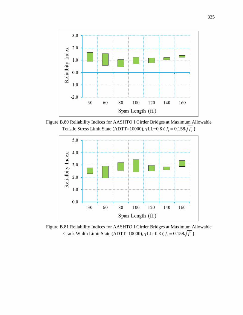
335
Figure B.80 Reliability Indices for AASHTO I Girder Bridges at Maximum Allowable
Tensile Stress Limit State (ADTT=10000), γLL=0.8 ( 0.158t cf f )
Figure B.81 Reliability Indices for AASHTO I Girder Bridges at Maximum Allowable
Crack Width Limit State (ADTT=10000), γLL=0.8 ( 0.158t cf f )
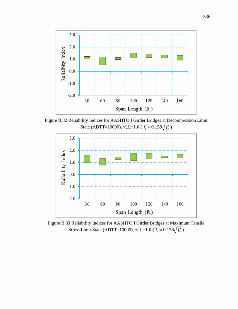
336
Figure B.82 Reliability Indices for AASHTO I Girder Bridges at Decompression Limit
State (ADTT=10000), γLL=1.0 ( 0.158t cf f )
Figure B.83 Reliability Indices for AASHTO I Girder Bridges at Maximum Tensile
Stress Limit State (ADTT=10000), γLL=1.0 ( 0.158t cf f )
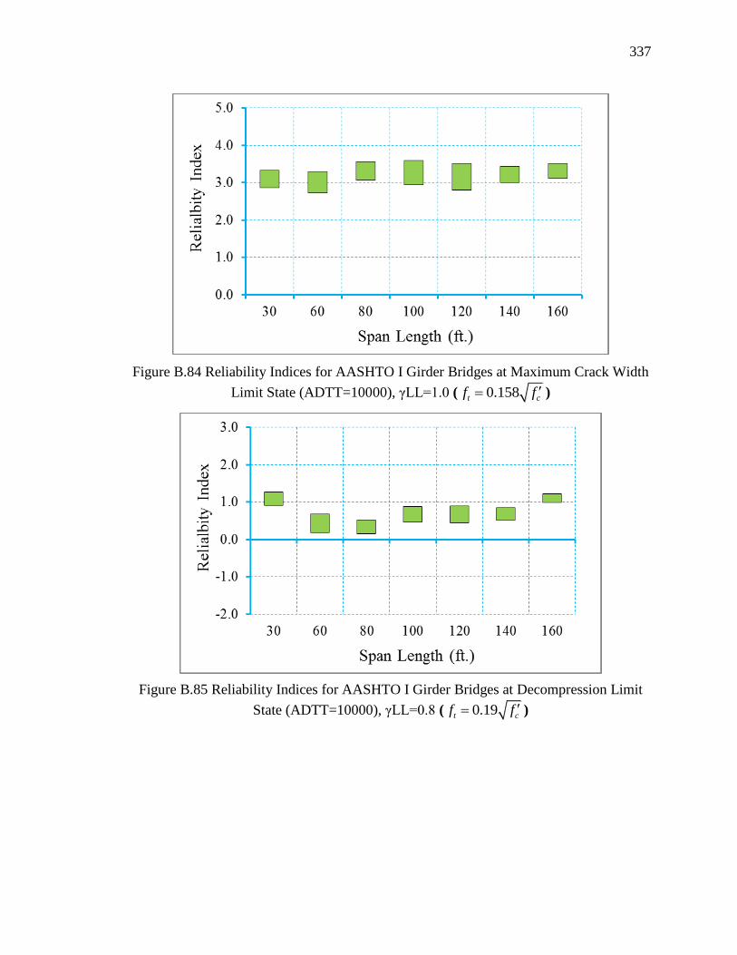
337
Figure B.84 Reliability Indices for AASHTO I Girder Bridges at Maximum Crack Width
Limit State (ADTT=10000), γLL=1.0 ( 0.158t cf f )
Figure B.85 Reliability Indices for AASHTO I Girder Bridges at Decompression Limit
State (ADTT=10000), γLL=0.8 ( 0.19t cf f )
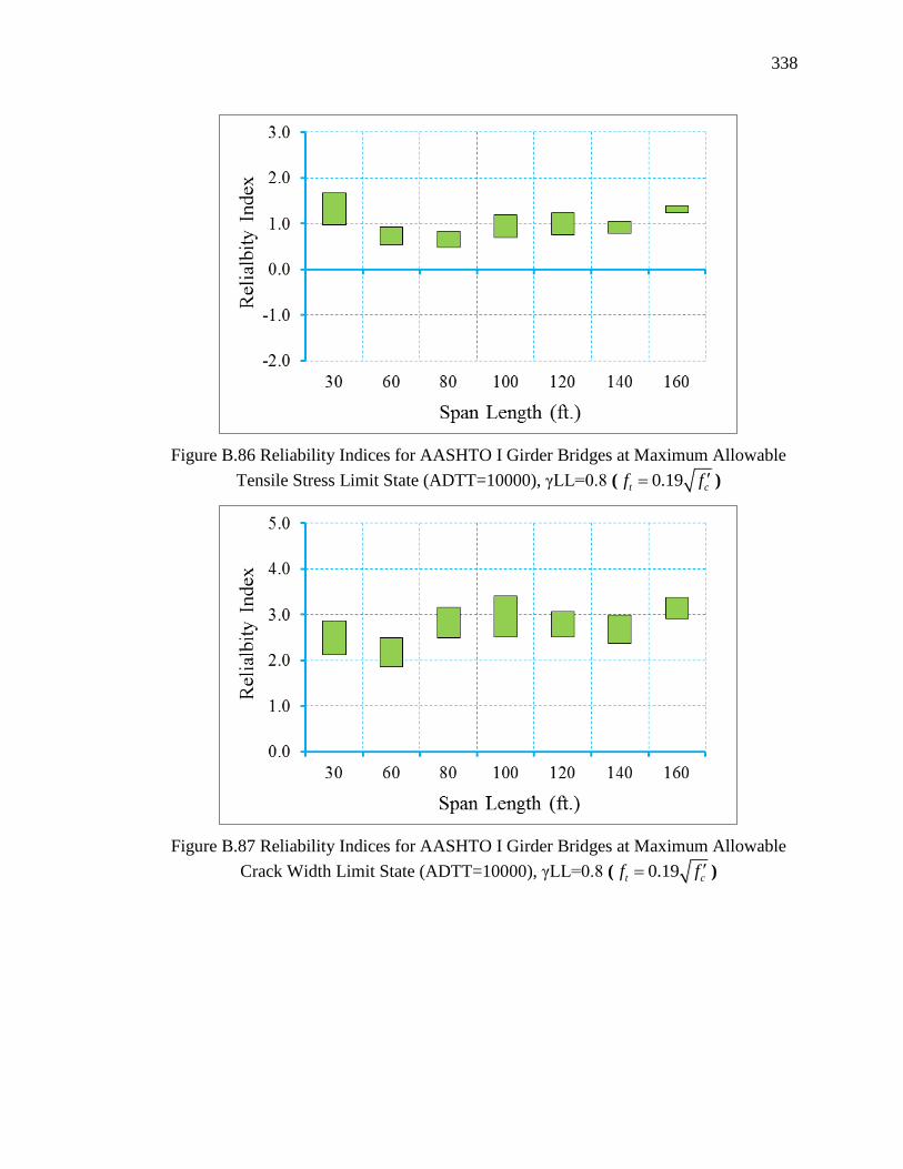
338
Figure B.86 Reliability Indices for AASHTO I Girder Bridges at Maximum Allowable
Tensile Stress Limit State (ADTT=10000), γLL=0.8 ( 0.19t cf f )
Figure B.87 Reliability Indices for AASHTO I Girder Bridges at Maximum Allowable
Crack Width Limit State (ADTT=10000), γLL=0.8 ( 0.19t cf f )
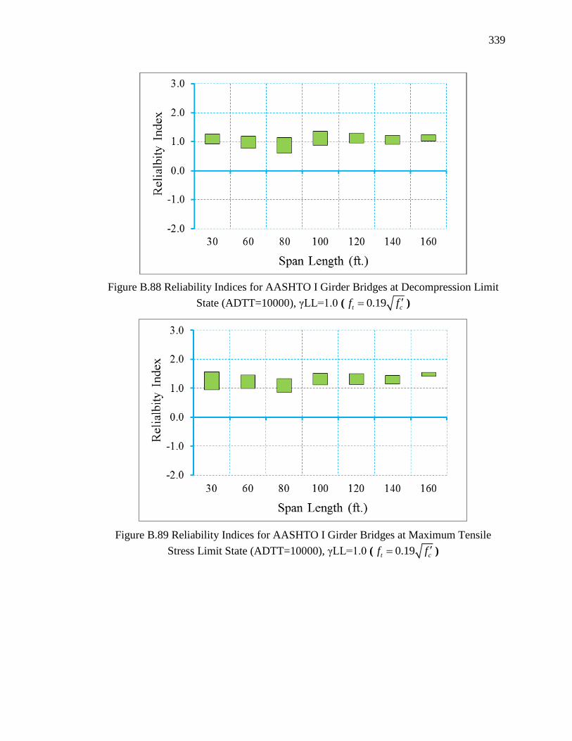
339
Figure B.88 Reliability Indices for AASHTO I Girder Bridges at Decompression Limit
State (ADTT=10000), γLL=1.0 ( 0.19t cf f )
Figure B.89 Reliability Indices for AASHTO I Girder Bridges at Maximum Tensile
Stress Limit State (ADTT=10000), γLL=1.0 ( 0.19t cf f )
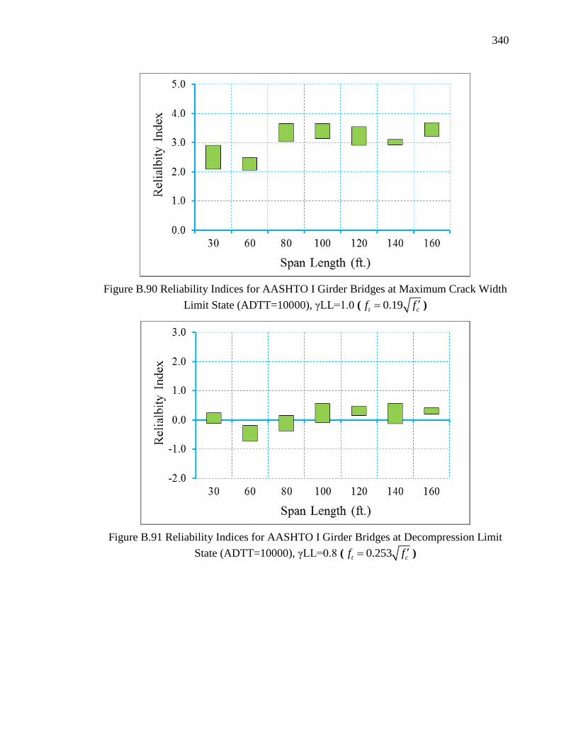
340
Figure B.90 Reliability Indices for AASHTO I Girder Bridges at Maximum Crack Width
Limit State (ADTT=10000), γLL=1.0 ( 0.19t cf f )
Figure B.91 Reliability Indices for AASHTO I Girder Bridges at Decompression Limit
State (ADTT=10000), γLL=0.8 ( 0.253t cf f )
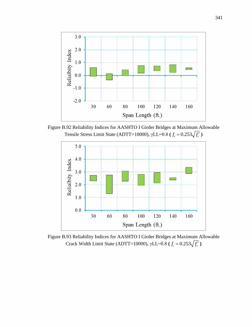
341
Figure B.92 Reliability Indices for AASHTO I Girder Bridges at Maximum Allowable
Tensile Stress Limit State (ADTT=10000), γLL=0.8 ( 0.253t cf f )
Figure B.93 Reliability Indices for AASHTO I Girder Bridges at Maximum Allowable
Crack Width Limit State (ADTT=10000), γLL=0.8 ( 0.253t cf f )
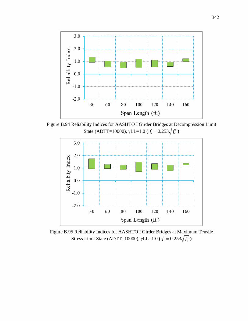
342
Figure B.94 Reliability Indices for AASHTO I Girder Bridges at Decompression Limit
State (ADTT=10000), γLL=1.0 ( 0.253t cf f )
Figure B.95 Reliability Indices for AASHTO I Girder Bridges at Maximum Tensile
Stress Limit State (ADTT=10000), γLL=1.0 ( 0.253t cf f )
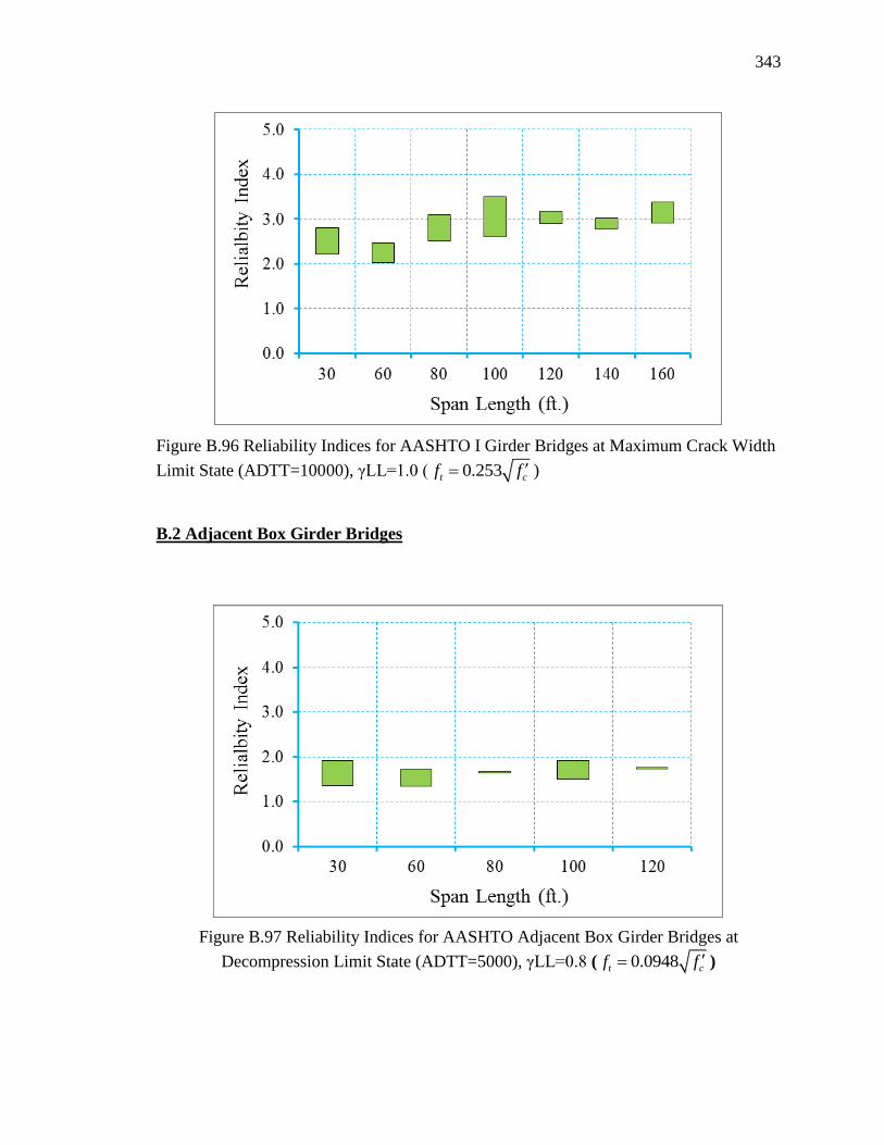
343
Figure B.96 Reliability Indices for AASHTO I Girder Bridges at Maximum Crack Width
Limit State (ADTT=10000), γLL=1.0 ( 0.253t cf f )
B.2 Adjacent Box Girder Bridges
Figure B.97 Reliability Indices for AASHTO Adjacent Box Girder Bridges at
Decompression Limit State (ADTT=5000), γLL=0.8 ( 0.0948t cf f )
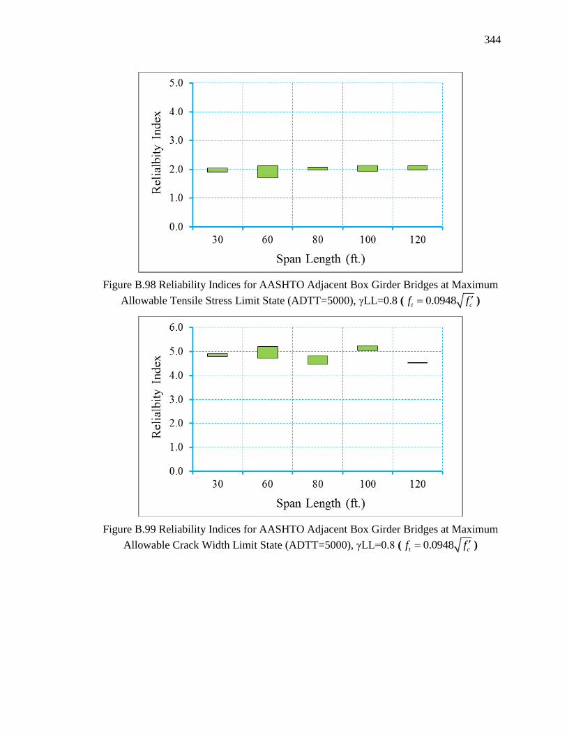
344
Figure B.98 Reliability Indices for AASHTO Adjacent Box Girder Bridges at Maximum
Allowable Tensile Stress Limit State (ADTT=5000), γLL=0.8 ( 0.0948t cf f )
Figure B.99 Reliability Indices for AASHTO Adjacent Box Girder Bridges at Maximum
Allowable Crack Width Limit State (ADTT=5000), γLL=0.8 ( 0.0948t cf f )

345
Figure B.100 Reliability Indices for AASHTO Adjacent Box Girder Bridges at
Decompression Limit State (ADTT=5000), γLL=1.0 ( 0.0948t cf f )
Figure B.101 Reliability Indices for AASHTO Adjacent Box Girder Bridges at Maximum
Tensile Stress Limit State (ADTT=5000), γLL=1.0 ( 0.0948t cf f )

346
Figure B.102 Reliability Indices for AASHTO Adjacent Box Girder Bridges at Maximum
Crack Width Limit State (ADTT=5000), γLL=1.0 ( 0.0948t cf f )
Figure B.103 Reliability Indices for AASHTO Adjacent Box Girder Bridges at
Decompression Limit State (ADTT=5000), γLL=0.8 ( 0.158t cf f )
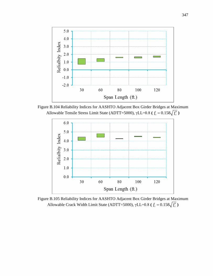
347
Figure B.104 Reliability Indices for AASHTO Adjacent Box Girder Bridges at Maximum
Allowable Tensile Stress Limit State (ADTT=5000), γLL=0.8 ( 0.158t cf f )
Figure B.105 Reliability Indices for AASHTO Adjacent Box Girder Bridges at Maximum
Allowable Crack Width Limit State (ADTT=5000), γLL=0.8 ( 0.158t cf f )
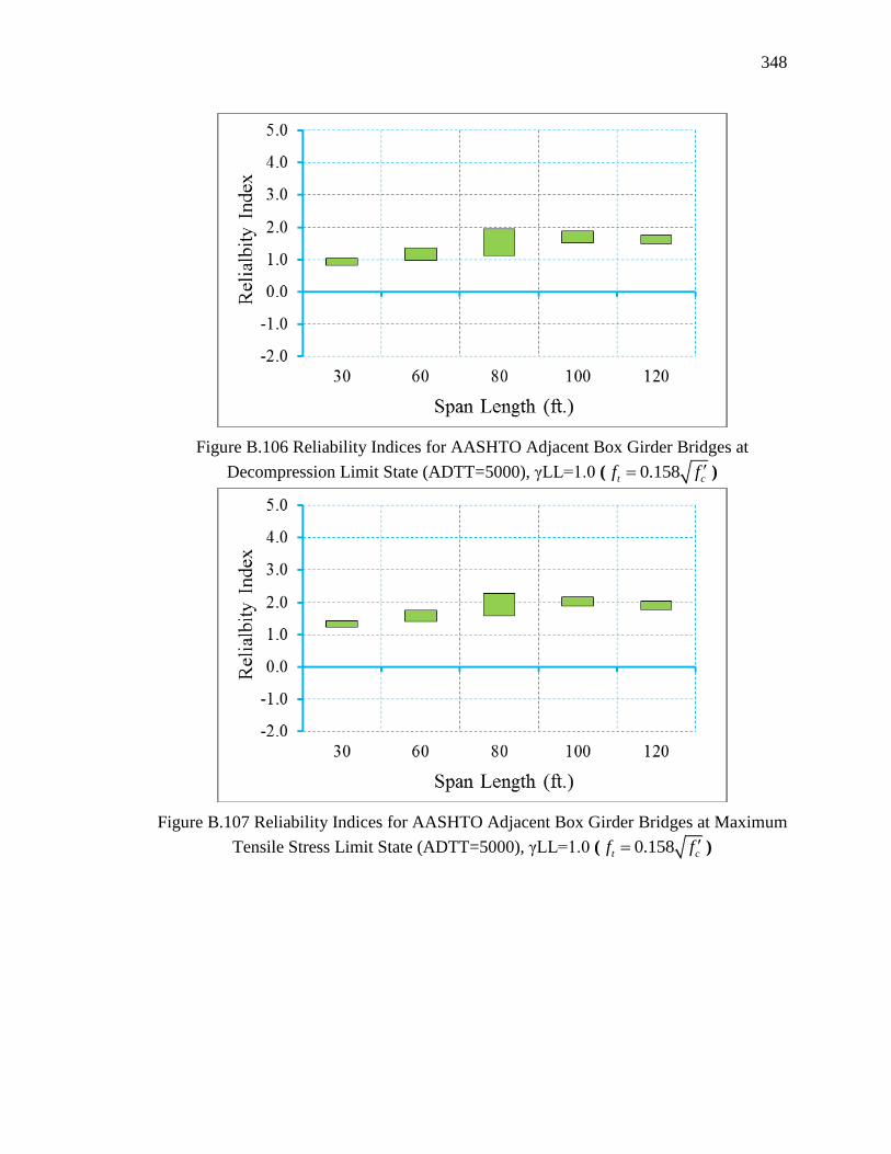
348
Figure B.106 Reliability Indices for AASHTO Adjacent Box Girder Bridges at
Decompression Limit State (ADTT=5000), γLL=1.0 ( 0.158t cf f )
Figure B.107 Reliability Indices for AASHTO Adjacent Box Girder Bridges at Maximum
Tensile Stress Limit State (ADTT=5000), γLL=1.0 ( 0.158t cf f )

349
Figure B.108 Reliability Indices for AASHTO Adjacent Box Girder Bridges at Maximum
Crack Width Limit State (ADTT=5000), γLL=1.0 ( 0.158t cf f )
Figure B.109 Reliability Indices for AASHTO Adjacent Box Girder Bridges at
Decompression Limit State (ADTT=5000), γLL=0.8 ( 0.19t cf f )
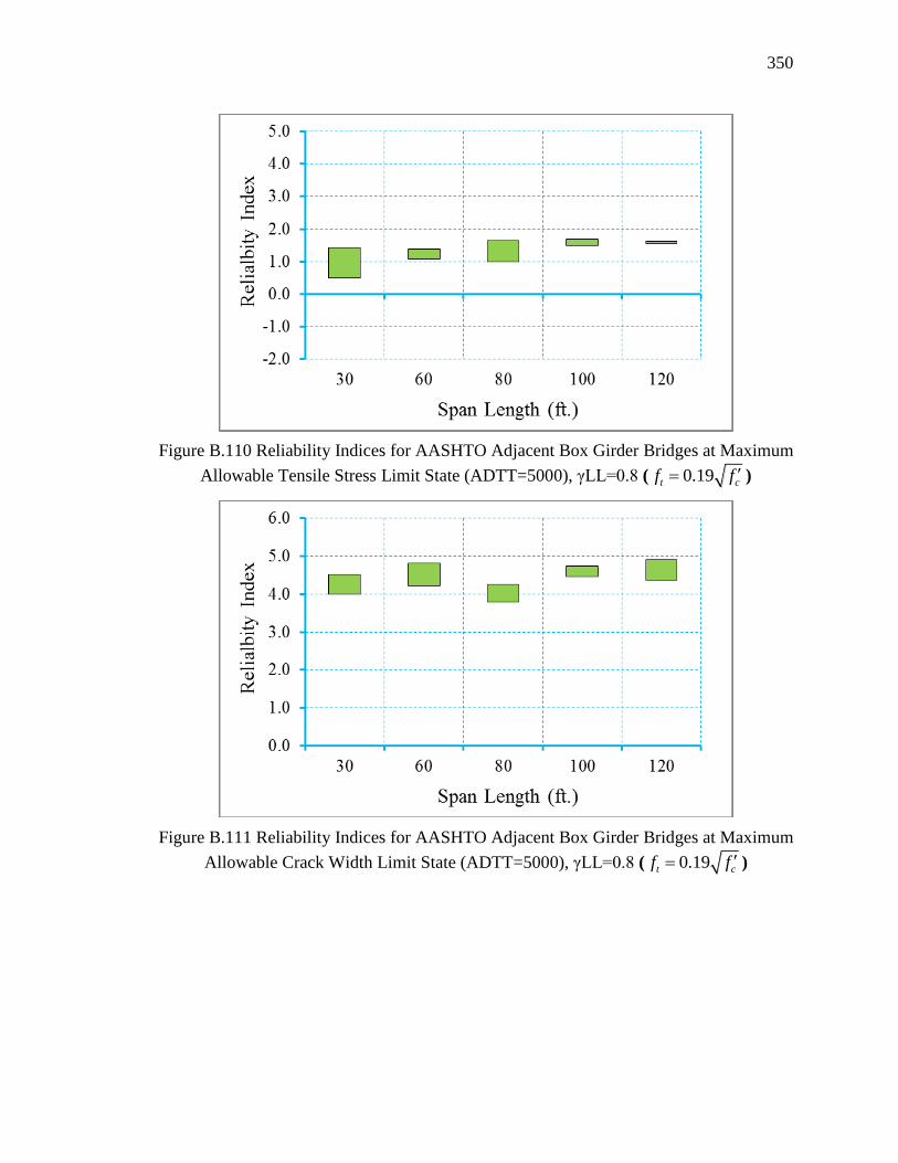
350
Figure B.110 Reliability Indices for AASHTO Adjacent Box Girder Bridges at Maximum
Allowable Tensile Stress Limit State (ADTT=5000), γLL=0.8 ( 0.19t cf f )
Figure B.111 Reliability Indices for AASHTO Adjacent Box Girder Bridges at Maximum
Allowable Crack Width Limit State (ADTT=5000), γLL=0.8 ( 0.19t cf f )
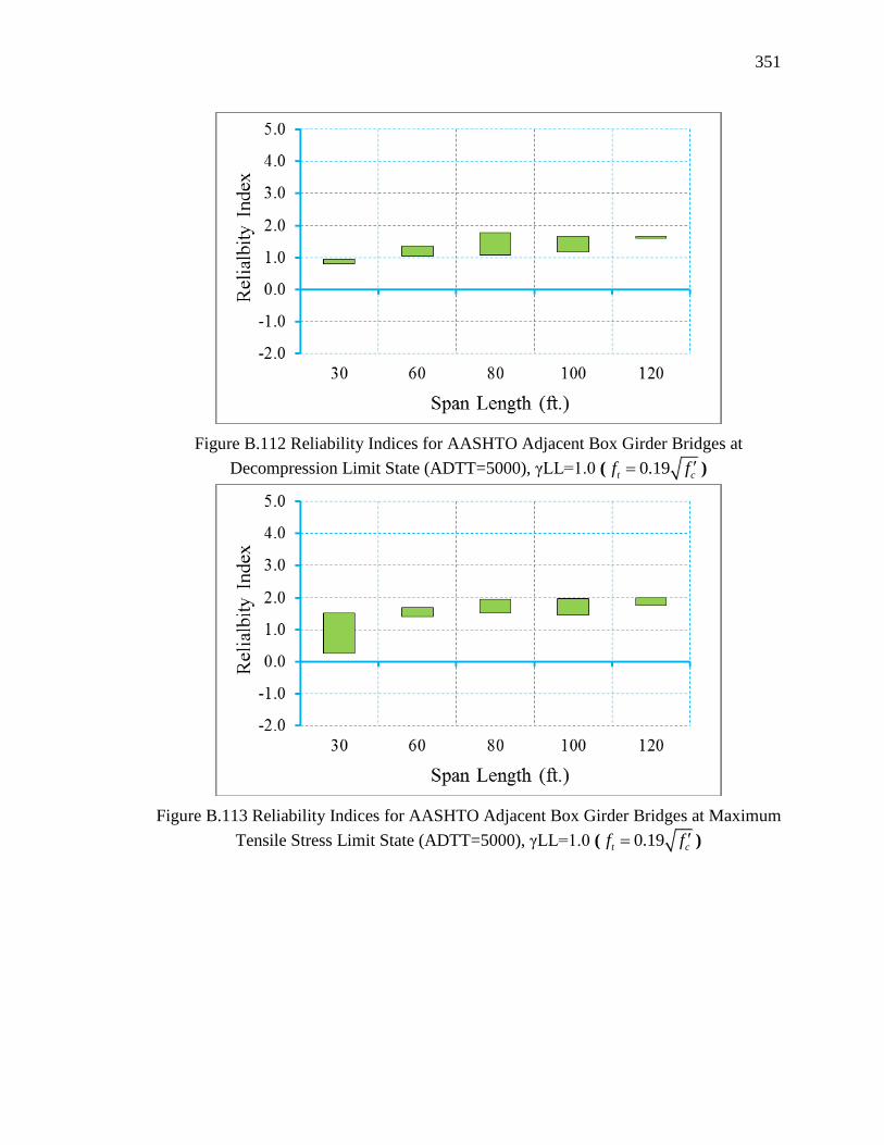
351
Figure B.112 Reliability Indices for AASHTO Adjacent Box Girder Bridges at
Decompression Limit State (ADTT=5000), γLL=1.0 ( 0.19t cf f )
Figure B.113 Reliability Indices for AASHTO Adjacent Box Girder Bridges at Maximum
Tensile Stress Limit State (ADTT=5000), γLL=1.0 ( 0.19t cf f )

352
Figure B.114 Reliability Indices for AASHTO Adjacent Box Girder Bridges at Maximum
Crack Width Limit State (ADTT=5000), γLL=1.0 ( 0.19t cf f )
Figure B.115 Reliability Indices for AASHTO Adjacent Box Girder Bridges at
Decompression Limit State (ADTT=5000), γLL=0.8 ( 0.253t cf f )
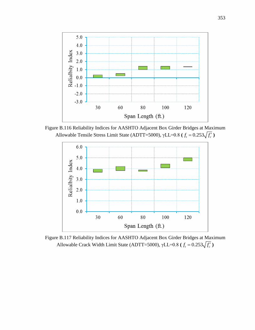
353
Figure B.116 Reliability Indices for AASHTO Adjacent Box Girder Bridges at Maximum
Allowable Tensile Stress Limit State (ADTT=5000), γLL=0.8 ( 0.253t cf f )
Figure B.117 Reliability Indices for AASHTO Adjacent Box Girder Bridges at Maximum
Allowable Crack Width Limit State (ADTT=5000), γLL=0.8 ( 0.253t cf f )
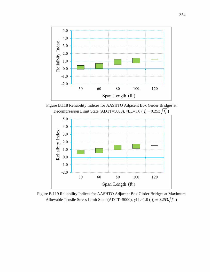
354
Figure B.118 Reliability Indices for AASHTO Adjacent Box Girder Bridges at
Decompression Limit State (ADTT=5000), γLL=1.0 ( 0.253t cf f )
Figure B.119 Reliability Indices for AASHTO Adjacent Box Girder Bridges at Maximum
Allowable Tensile Stress Limit State (ADTT=5000), γLL=1.0 ( 0.253t cf f )
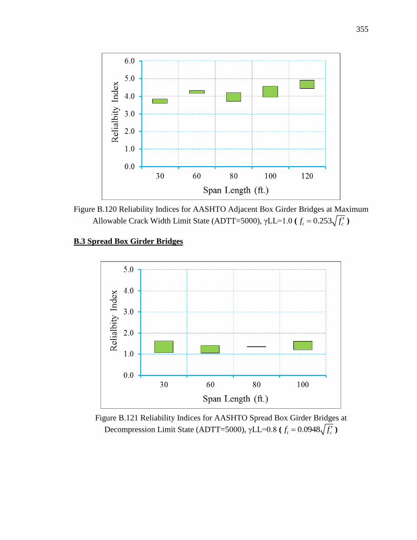
355
Figure B.120 Reliability Indices for AASHTO Adjacent Box Girder Bridges at Maximum
Allowable Crack Width Limit State (ADTT=5000), γLL=1.0 ( 0.253t cf f )
B.3 Spread Box Girder Bridges
Figure B.121 Reliability Indices for AASHTO Spread Box Girder Bridges at
Decompression Limit State (ADTT=5000), γLL=0.8 ( 0.0948t cf f )

356
Figure B.122 Reliability Indices for AASHTO Spread Box Girder Bridges at Maximum
Allowable Tensile Stress Limit State (ADTT=5000), γLL=0.8 ( 0.0948t cf f )
Figure B.123 Reliability Indices for AASHTO Spread Box Girder Bridges at Maximum
Allowable Crack Width Limit State (ADTT=5000), γLL=0.8 ( 0.0948t cf f )

357
Figure B.124 Reliability Indices for AASHTO Spread Box Girder Bridges at
Decompression Limit State (ADTT=5000), γLL=1.0 ( 0.0948t cf f )
Figure B.125 Reliability Indices for AASHTO Spread Box Girder Bridges at Maximum
Tensile Stress Limit State (ADTT=5000), γLL=1.0 ( 0.0948t cf f )

358
Figure B.126 Reliability Indices for AASHTO Spread Box Girder Bridges at Maximum
Crack Width Limit State (ADTT=5000), γLL=1.0 ( 0.0948t cf f )
Figure B.127 Reliability Indices for AASHTO Spread Box Girder Bridges at
Decompression Limit State (ADTT=5000), γLL=0.8 ( 0.158t cf f )
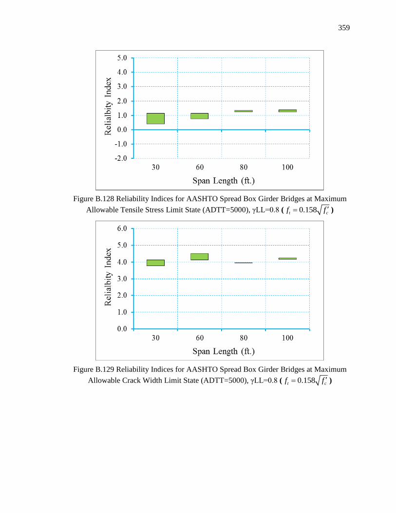
359
Figure B.128 Reliability Indices for AASHTO Spread Box Girder Bridges at Maximum
Allowable Tensile Stress Limit State (ADTT=5000), γLL=0.8 ( 0.158t cf f )
Figure B.129 Reliability Indices for AASHTO Spread Box Girder Bridges at Maximum
Allowable Crack Width Limit State (ADTT=5000), γLL=0.8 ( 0.158t cf f )

360
Figure B.130 Reliability Indices for AASHTO Spread Box Girder Bridges at
Decompression Limit State (ADTT=5000), γLL=1.0 ( 0.158t cf f )
Figure B.131 Reliability Indices for AASHTO Spread Box Girder Bridges at Maximum
Tensile Stress Limit State (ADTT=5000), γLL=1.0 ( 0.158t cf f )
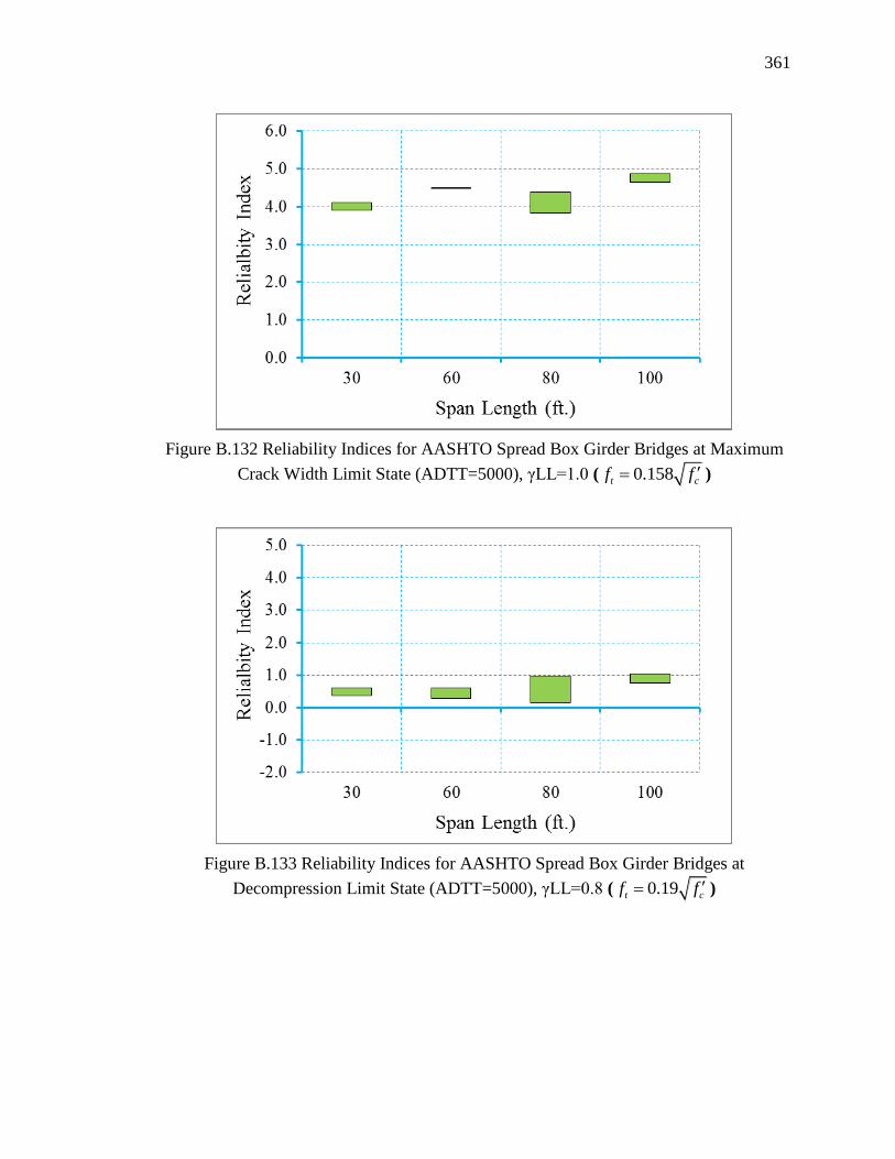
361
Figure B.132 Reliability Indices for AASHTO Spread Box Girder Bridges at Maximum
Crack Width Limit State (ADTT=5000), γLL=1.0 ( 0.158t cf f )
Figure B.133 Reliability Indices for AASHTO Spread Box Girder Bridges at
Decompression Limit State (ADTT=5000), γLL=0.8 ( 0.19t cf f )

362
Figure B.134 Reliability Indices for AASHTO Spread Box Girder Bridges at Maximum
Allowable Tensile Stress Limit State (ADTT=5000), γLL=0.8 ( 0.19t cf f )
Figure B.135 Reliability Indices for AASHTO Spread Box Girder Bridges at Maximum
Allowable Crack Width Limit State (ADTT=5000), γLL=0.8 ( 0.19t cf f )

363
Figure B.136 Reliability Indices for AASHTO Spread Box Girder Bridges at
Decompression Limit State (ADTT=5000) γLL=1.0 ( 0.19t cf f )
Figure B.137 Reliability Indices for AASHTO Spread Box Girder Bridges at Maximum
Tensile Stress Limit State (ADTT=5000), γLL=1.0 ( 0.19t cf f )

364
Figure B.138 Reliability Indices for AASHTO Spread Box Girder Bridges at Maximum
Crack Width Limit State (ADTT=5000), γLL=1.0 ( 0.19t cf f )
Figure B.139 Reliability Indices for AASHTO Spread Box Girder Bridges at
Decompression Limit State (ADTT=5000), γLL=0.8 ( 0.253t cf f )

365
Figure B.140 Reliability Indices for AASHTO Spread Box Girder Bridges at Maximum
Allowable Tensile Stress Limit State (ADTT=5000), γLL=0.8 ( 0.253t cf f )
Figure B.141 Reliability Indices for AASHTO Spread Box Girder Bridges at Maximum
Allowable Crack Width Limit State (ADTT=5000), γLL=0.8 ( 0.253t cf f )

366
Figure B.142 Reliability Indices for AASHTO Spread Box Girder Bridges at
Decompression Limit State (ADTT=5000), γLL=1.0 ( 0.253t cf f )
Figure B.143 Reliability Indices for AASHTO Spread Box Girder Bridges at Maximum
Allowable Tensile Stress Limit State (ADTT=5000), γLL=1.0 ( 0.253t cf f )
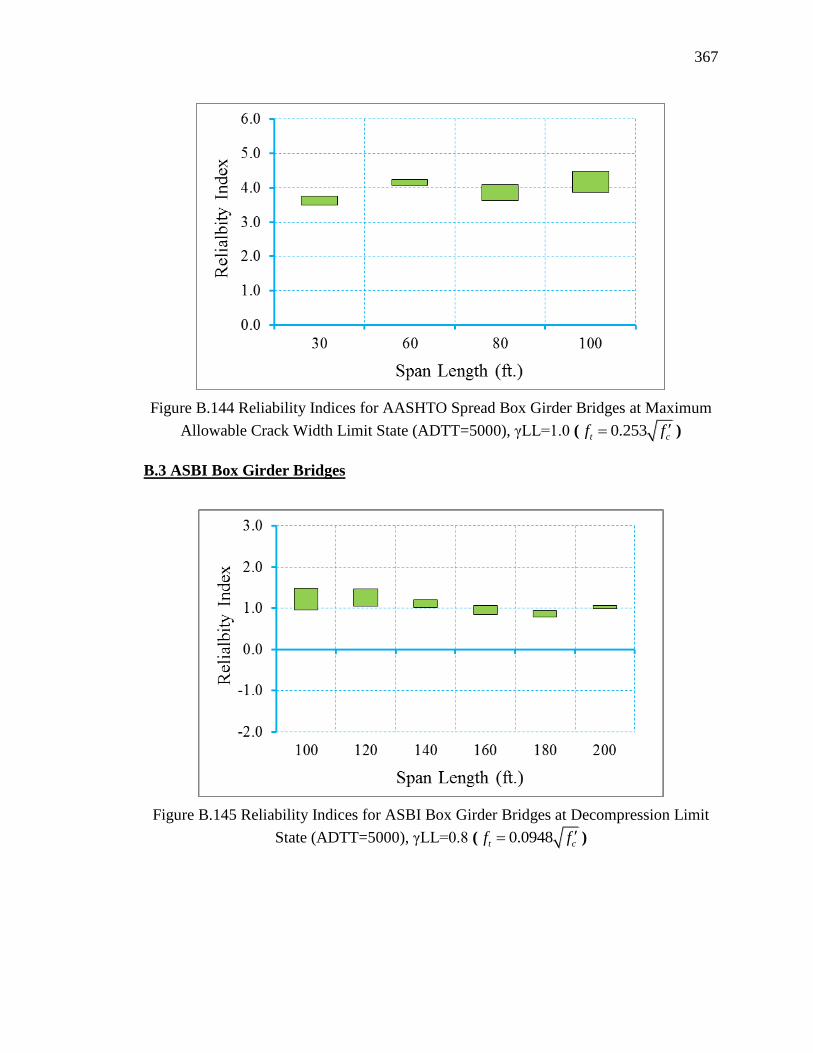
367
Figure B.144 Reliability Indices for AASHTO Spread Box Girder Bridges at Maximum
Allowable Crack Width Limit State (ADTT=5000), γLL=1.0 ( 0.253t cf f )
B.3 ASBI Box Girder Bridges
Figure B.145 Reliability Indices for ASBI Box Girder Bridges at Decompression Limit
State (ADTT=5000), γLL=0.8 ( 0.0948t cf f )
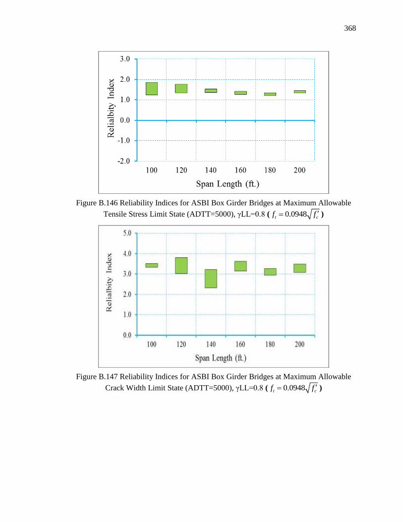
368
Figure B.146 Reliability Indices for ASBI Box Girder Bridges at Maximum Allowable
Tensile Stress Limit State (ADTT=5000), γLL=0.8 ( 0.0948t cf f )
Figure B.147 Reliability Indices for ASBI Box Girder Bridges at Maximum Allowable
Crack Width Limit State (ADTT=5000), γLL=0.8 ( 0.0948t cf f )

369
Figure B.148 Reliability Indices for ASBI Box Girder Bridges at Decompression Limit
State (ADTT=5000), γLL=1.0 ( 0.0948t cf f )
Figure B.149 Reliability Indices for ASBI Box Girder Bridges at Maximum Tensile
Stress Limit State (ADTT=5000), γLL=1.0 ( 0.0948t cf f )
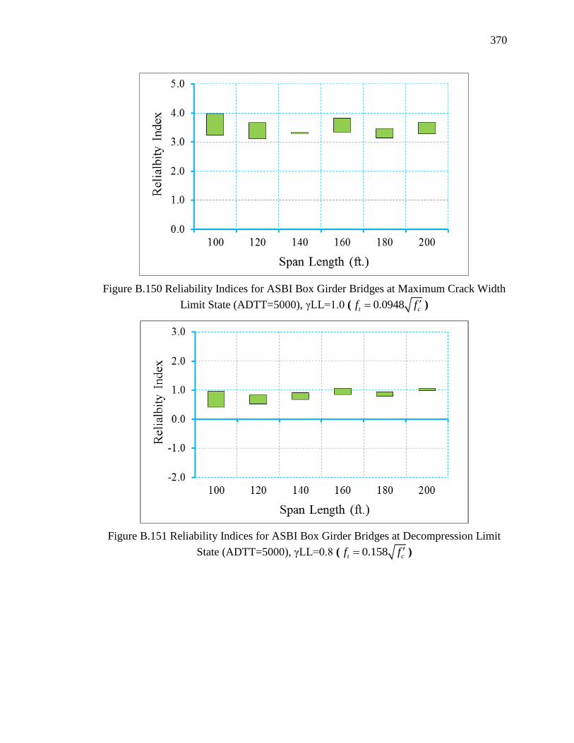
370
Figure B.150 Reliability Indices for ASBI Box Girder Bridges at Maximum Crack Width
Limit State (ADTT=5000), γLL=1.0 ( 0.0948t cf f )
Figure B.151 Reliability Indices for ASBI Box Girder Bridges at Decompression Limit
State (ADTT=5000), γLL=0.8 ( 0.158t cf f )

371
Figure B.152 Reliability Indices for ASBI Box Girder Bridges at Maximum Allowable
Tensile Stress Limit State (ADTT=5000), γLL=0.8 ( 0.158t cf f )
Figure B.153 Reliability Indices for ASBI Box Girder Bridges at Maximum Allowable
Crack Width Limit State (ADTT=5000), γLL=0.8 ( 0.158t cf f )

372
Figure B.154 Reliability Indices for ASBI Box Girder Bridges at Decompression Limit
State (ADTT=5000), γLL=1.0 ( 0.158t cf f )
Figure B.155 Reliability Indices for ASBI Box Girder Bridges at Maximum Tensile
Stress Limit State (ADTT=5000), γLL=1.0 ( 0.158t cf f )

373
Figure B.156 Reliability Indices for ASBI Box Girder Bridges at Maximum Crack Width
Limit State (ADTT=5000), γLL=1.0 ( 0.158t cf f )
Figure B.157 Reliability Indices for ASBI Box Girder Bridges at Decompression Limit
State (ADTT=5000), γLL=0.8 ( 0.19t cf f )
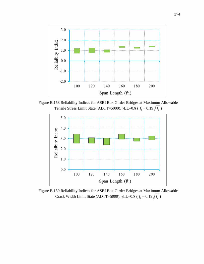
374
Figure B.158 Reliability Indices for ASBI Box Girder Bridges at Maximum Allowable
Tensile Stress Limit State (ADTT=5000), γLL=0.8 ( 0.19t cf f )
Figure B.159 Reliability Indices for ASBI Box Girder Bridges at Maximum Allowable
Crack Width Limit State (ADTT=5000), γLL=0.8 ( 0.19t cf f )
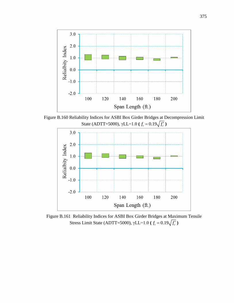
375
Figure B.160 Reliability Indices for ASBI Box Girder Bridges at Decompression Limit
State (ADTT=5000), γLL=1.0 ( 0.19t cf f )
Figure B.161 Reliability Indices for ASBI Box Girder Bridges at Maximum Tensile
Stress Limit State (ADTT=5000), γLL=1.0 ( 0.19t cf f )
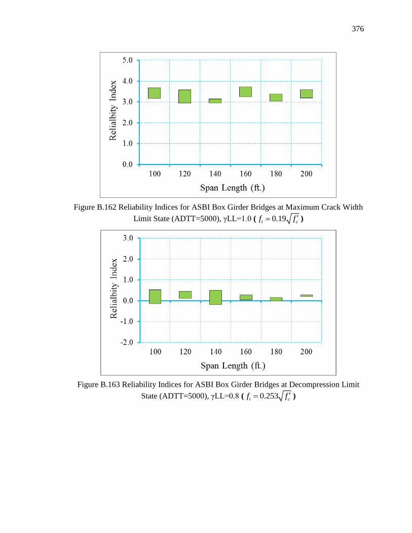
376
Figure B.162 Reliability Indices for ASBI Box Girder Bridges at Maximum Crack Width
Limit State (ADTT=5000), γLL=1.0 ( 0.19t cf f )
Figure B.163 Reliability Indices for ASBI Box Girder Bridges at Decompression Limit
State (ADTT=5000), γLL=0.8 ( 0.253t cf f )
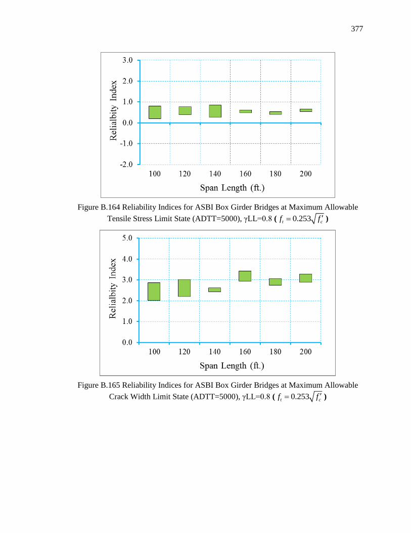
377
Figure B.164 Reliability Indices for ASBI Box Girder Bridges at Maximum Allowable
Tensile Stress Limit State (ADTT=5000), γLL=0.8 ( 0.253t cf f )
Figure B.165 Reliability Indices for ASBI Box Girder Bridges at Maximum Allowable
Crack Width Limit State (ADTT=5000), γLL=0.8 ( 0.253t cf f )

378
Figure B.166 Reliability Indices for ASBI Box Girder Bridges at Decompression Limit
State (ADTT=5000), γLL=1.0 ( 0.253t cf f )
Figure B.167 Reliability Indices for ASBI Box Girder Bridges at Maximum Allowable
Tensile Stress Limit State (ADTT=5000), γLL=1.0 ( 0.253t cf f )
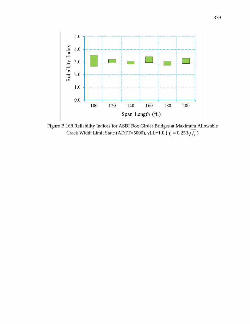
379
Figure B.168 Reliability Indices for ASBI Box Girder Bridges at Maximum Allowable
Crack Width Limit State (ADTT=5000), γLL=1.0 ( 0.253t cf f )