© 2013 rahul agarwal
TRANSCRIPT

© 2013 Rahul Agarwal

MODELING HEAT REJECTION IN HORIZONTAL SMOOTH ROUND TUBES AND
EXPERIMENTAL VALIDATION FOR R1234ze(E), R134a AND R32
BY
RAHUL AGARWAL
THESIS
Submitted in partial fulfillment of the requirements
for the degree of Master of Science in Mechanical Engineering
in the Graduate College of the
University of Illinois at Urbana-Chamapaign, 2013
Urbana, Illinois
Adviser:
Professor Predrag S. Hrnjak

ii
ABSTRACT
Heat transfer in condensers is typically divided into 3 zones: superheated, two-phase and
sub cooled region. These regions, in general, are considered to be independent of each other and
various correlations are available in literature to predict the heat transfer coefficient (HTC) in
these regions separately. These correlations, if plotted as a function of quality for the three
regions, will show discontinuity at qualities of 0 and 1. The aim of the thesis is to bridge the
discontinuity by establishing the interdependency of these regions and propose a unified model
to predict HTC throughout the condensers. Experimental data suggests the HTC near x=1 in de-
superheating region to be significantly higher than predictions due to presence of liquid when the
wall temperature drops below saturation temperature. Similarly, HTC below x=0 has been seen
to decrease linearly before following Gnielinski correlation due to presence of vapor as seen in
sight glass at the end of test section. The newly proposed model takes into account the presence
of liquid in de-superheating and sub-cooled liquid in two-phase zone. The model has been
developed independently and compared to experimental data for R134a, R1234ze(E) and R32 for
mass fluxes of 100-300 kgm-2
s-1
, saturation temperatures of 30 0C - 50
0C and from sub-cooling
of 20 0C to superheat of 50
0C in a horizontal smooth tube with 6.1 mm inner diameter. Cavallini
et al. (2006) and Gnielinski correlations have been used as a baseline correlation to calculate
HTC in two-phase and single phase zone respectively. The model predicts the HTC satisfactorily
within an accuracy of 16 %.
Another objective of the work is to form a baseline for the heat transfer characteristics in
condensation for R1234ze(E) which can be a potential replacement in automotive systems for
R134a on account of low GWP. The properties of R1234ze(E) is fairly well know to be close to
R134a, however, the performance data under similar operating conditions as R134a is not widely
published. To enhance the performance, the use of refrigerant mixture is also a possibility.
Hence, R32 which is known to have higher heat transfer coefficient for its favorable thermo
physical properties is a viable option to be considered as a mixture with R1234ze with a trade-off
in GWP. Experiments conducted for R134a, R1234ze(E) and R32 at various mass fluxes,
saturation temperature and heat fluxes helps in analyzing the effect of various parameters on heat
transfer coefficient. The work in this thesis can be used as reference to study the effect of
mixtures on heat transfer coefficient.

iii
To my parents and my brother

iv
ACKNOWLEDGEMENTS
It gives me immense pleasure to acknowledge the individuals who made this research
possible. I would like to start by expressing my gratitude towards my adviser Professor Predrag
S. Hrnjak for his constant support, guidance and motivation throughout the project. His insights
and flexibility for a new approach helped me evolve as a researcher. I could not have imagined a
better professor or a better person to be my adviser.
I would take this opportunity to thank my colleagues Huize Li, Han Fe, Augusto
Zimmerman, Aravind Ramakrishnan, Bharath Budhiraja, Yang Zou, Shenghan Jin, Neal
Lawrence, Melissa Meyers and Chieko Kondou who always helped my when I got stuck and
made this journey a memorable one. A special mention goes to Rahul Kolekar whose expertise in
experiments was of tremendous help. I would also like to thank all the sponsors of ACRC for
their support and guidance in this project.
I would like to acknowledge the moral support of my friends Dinkar Nandwana, Arpit
Agarwal, Rajavasanth Rajasegar, Subhabrata Banerjee and Ashwin Bhardwaj who encouraged
me in trying times and ensured that I had friends whom I can count upon in the hour of need.
Last but not the least I would like to thank my parents and my brother for their love and
support throughout my life. They have made me what I am today and I owe them everything I
have done and will do in my life.

v
TABLE OF CONTENTS
LIST OF SYMBOLS .................................................................................................................... vii
CHAPTER 1: INTRODUCTION ....................................................................................................1
1.1 Background ..........................................................................................................................1
1.2 Literature Review.................................................................................................................2
1.2.1 Condensation in Superheated Zone ............................................................................2
1.2.2 Condensation in Two Phase Zone...............................................................................3
1.2.3 Condensation in Sub-Cooled zone ..............................................................................5
1.2.4 Condensation of R1234ze(E) ......................................................................................5
1.3 Research Objectives .............................................................................................................6
CHAPTER 2: MODELING OF HEAT TRANSFER IN CONDENSERS .....................................7
2.1 Conventional Approach in Modeling of Heat Rejection ....................................................7
2.1.1 Condensation in Superheated Zone ............................................................................9
2.1.2 Condensation in Two Phase Zone...............................................................................9
2.1.3 Condensation in Sub-Cooled Zone .............................................................................9
2.2 Principle of Heat Rejection in Condensers ........................................................................11
2.3 Heat Transfer Model Proposed ..........................................................................................12
2.3.1 Assumptions ..............................................................................................................13
2.3.2 De-Superheating Zone ..............................................................................................13
2.3.3 Condensing Superheat Zone .....................................................................................14
2.3.4 Two Phase Zone ........................................................................................................15
2.3.5 Sub-Cooled Zone ......................................................................................................17
2.4 Calculation Procedure ........................................................................................................18
CHAPTER 3: EXPERIMENTAL METHOD ...............................................................................19
3.1 Facility for Experiments ....................................................................................................19
3.2 Test Section ........................................................................................................................20
3.3 Experimental Measurement and Uncertainties ..................................................................20
3.4 Range of test conditions .....................................................................................................21

vi
3.5 Data reduction procedure ...................................................................................................22
CHAPTER 4: RESULTS AND DISCUSSION .............................................................................24
4.1 Smooth Transition of HTC across Superheated, Two Phase and Sub-Cooled Zone .........24
4.1.1 Condensation in Superheated Zone ..........................................................................26
4.1.2 Condensation in Two Phase Zone.............................................................................26
4.1.3 Condensation in Sub-Cooled Zone ...........................................................................26
4.2 Effect of Parameters on Heat Transfer Coefficient ............................................................30
4.2.1 Effect of Mass Flux ...................................................................................................30
4.2.2 Effect of Heat Flux....................................................................................................31
4.2.3 Effect of Saturation Temperature..............................................................................31
4.3 Comparison of HTC for Different Refrigerants .................................................................33
4.3.1 Heat Transfer Coefficient .........................................................................................33
4.3.2 Pressure Drop ............................................................................................................33
4.4 Comparison of experimental data to prediction .................................................................35
4.4.1 Comparison to Correlations from Literature.............................................................35
4.4.2 Comparison to the Proposed Model ..........................................................................38
4.5 Summary of Experimental Results ....................................................................................42
CHAPTER 5: SUMMARY, CONCLUSIONS AND RECOMMENDATIONS ..........................44
3.1 Summary and Concluding Remarks ..................................................................................44
3.2 Recommendations for Future Study ..................................................................................46
APPENDIX A: CALIBRATION RESULTS ................................................................................47
APPENDIX B: REPEATABILITY TESTS ..................................................................................54
APPENDIX C: UNCERTAINTY ANALYSIS .............................................................................58
APPENDIX D: EXPERIMENTAL DATA ...................................................................................63
REFERENCES ..............................................................................................................................75

vii
LIST OF SYMBOLS
A Surface area [m2]
Cp Specific heat capacity [Jkg-1
K-1
]
di Inner diameter of test tube [m]
fb Friction factor [-]
g Gravitational acceleration [ms-2
]
G Mass flux [kgm-2
s-1
]
GWP Global Warming Potential [-]
h Specific Enthalpy [Jkg-1
]
∆hlv Latent heat [Jkg-1
]
HMFR Heat Mass Flux Ratio [-]
HTC See α [Wm-2
K-1
]
J Dimensionless gas velocity [-]
Greek Symbols
ρ Density [kgm-3
]
µ Viscosity [Pa.s]
λ Thermal Conductivity [Wm-1
K-1
]
σ Surface Tension [Nm-1
]
δ Film thickness [m]
θ Angle [rad]
ε Void fraction [-]
α Heat Transfer Coefficient [Wm-2
s-1
]
JT Transition gas velocity [-]
ṁ Mass flow rate [kgs-1
]
Nu Nusselt number [-]
P Pressure [Pa]
Pr Prandtl number [-]
Heat transfer rate [W]
q Heat flux [Wm-2
]
Re Reynolds number [-]
T Temperature [0C]
X Vapor quality [-]
X Lockhart-Martinelli parameter [-]
∆Z Cooling length of test tube [m]

viii
Subscripts
Air Evaluated for air
b Evaluated at bulk temperature
cond Conduction heat from test section
f Evaluated at film temperature
G Gas phase
gain Heat gain from ambient
H2O Water
i Inlet
L Liquid
Latent Latent heat
LO Liquid phase with total flow
MC Mixing chamber
O Outlet
Subscripts
PC Pre cooler
R Refrigerant
Sat Evaluated at saturation temperature
SC Sub-cool
Sensible Sensible heat
SH Superheat
Strat Fully stratified flow regime
Total Toal heat transfer
TP Two phase
TS Test Section
Tt Turbulent-turbulent
V Vapor
W Wall

1
CHAPTER 1
INTRODUCTION
1.1 Background
Heat transfer in condensers is usually modeled in the two-phase zone with various
correlations predicting heat transfer coefficient as a function of quality. While there are abundant
correlations to predict heat transfer in two phase zone, heat transfer coefficient (HTC) in single
phase is predicted with fairly high accuracy with Dittus-Boelter and Gneillinski correlations
assuming single phase turbulent conditions. These correlations, if plotted as a function of
enthalpy shows discontinuity between single phase and two phase zones. This discontinuity
arises because the models implicitly assume thermodynamic equilibrium during condensation
which indicates that the first drop of condensate would form when bulk enthalpy of vapor
reaches saturation enthalpy. Experimental studies have been conducted to prove that the heat
transfer coefficient starts deviating from the predictions of single phase correlations when the
wall temperature drops below saturation temperature and approaches the predictions of two-
phase correlations when bulk enthalpy equals saturation enthalpy. The models proposed in
literature also presume the temperature of liquid in two-phase zone to be saturation temperature
due to which the two phase correlations do not asymptotically satisfy the single phase heat
transfer data at qualities equal to 0. It has been shown experimentally that the liquid in two-phase
zone is sub-cooled and there is a smooth transition of HTC from two-phase to single phase zone.
A model has been proposed which takes both these phenomena into account to explain the
transition from single phase to two phase zones and vice-versa.
As per the Kyoto protocol (11 December 1997) industries are striving towards replacing
R134a with new refrigerants with low GWP which can reduce the carbon-dioxide emission in
atmosphere. However, it is not possible to design entirely new systems for the new refrigerants
owing to enormous cost associated with it. Hence, efforts have been made towards finding a
refrigerant which can be used simply as a drop-in replacement for R134a which led to the
discovery of two major refrigerants, R1234yf and R1234ze with properties very close to R134a.
The research work deals with establishing baseline heat transfer performance for R1234ze(E) in
condensers as the data available in literature currently is limited. The heat transfer coefficients of

2
R1234ze(E) are also compared to R134a to see the effect of replacement on the system. In order
to increase the heat transfer coefficient in condensers R1234ze(E) can be mixed with R32 which
has higher heat transfer coefficients because of its favorable thermo-physical properties. Hence, a
baseline data for heat transfer has also been taken for R32 which can be used as a reference when
compared to the mixture of R1234ze(E) and R32.
1.2 Literature Review:
1.2.1 Condensation in Superheated Zone
Heat transfer in condensers is usually modeled in the two-phase zone with various
correlations predicting heat transfer coefficient as a function of quality. These models implicitly
assume thermodynamic equilibrium during condensation which indicates that the first drop of
condensate would form when bulk enthalpy of vapor reaches saturation enthalpy. This
assumption has been proved to be incorrect as the phenomena of condensation in superheated
zone has been known and accepted in literature for many years. The effect, however, has not
been quantified by many. Kondou and Hrnjak (2012) identified the presence of condensation in
superheated region for CO2. They conducted experiments near critical point which magnified the
importance of condensation in superheated zone since the latent heat is very small near critical
pressure where even single phase correlations predict reality a bit better than two phase
correlations for lower reduced pressures. The deviation from superheat was explained using von-
Karman universal temperature profile which determined the magnitude of sub-cooling based on
measured wall temperature. Kondou and Hrnjak (2011b) also conducted experiments with
R410A and termed the region exhibiting condensation in superheated zone (SH) as Condensing
Superheated Zone (CSH). The HTC in CSH zone was shown to be much higher compared to the
prediction by Gnielinski correlation. The Kondo-Hrnjak correlation was then proposed based on
the argument that the heat rejection in CSH zone is a combination of sensible and latent heat.
The correlation was compared to experimental data for CO2 and R410A at mass fluxes of 100-
240 kgm-2
s-1
and reduced pressure of .68-1.0 in horizontal tubes which showed satisfactory
agreement. The criteria for beginning of condensation (Kondou and Hrnjak, 2011a) have been
identified to be the point where wall temperature drops below saturation temperature of the
refrigerant at corresponding operating condition. They determined the start of condensation to be

3
a strong function of heat flux arguing that greater heat flux results in lower wall temperature
which leads to earlier establishment of the criteria for condensation. Lee et al. (1991)
experimentally investigated condensation in superheated R22 vapor and proposed a model
accounting the sensible heat rejected in condensation heat transfer. Akers et al. (1959) developed
an in-tube condensation model with the help of equivalent Reynolds number. They defined an all
liquid flow rate that gave same heat transfer coefficient as an annular condensing flow. Webb
(1998) modified this model by expressing the HTC as a function of two-phase and single phase
HTC with the inclusion of the F-factor which asymptotically approaches 0 to satisfy the
boundary condition at x=1. Balekjian and Katz (1958) investigated film condensation of
superheated vapor on horizontal tubes for water and R114. They looked into the temperature
profile of refrigerant within the tube with both superheated vapor and liquid film existing
simultaneously. They defined interfacial film coefficient to be a measure of condensation at the
interface which was inversely proportional to the degree of superheat. A correlation was
proposed based on theory of inter-phase mass and energy transfer but it was said that more
experimental measurements are needed to thoroughly understand the phenomena occurring at
interface.
1.2.2 Condensation in Two Phase Zone
Condensation heat transfer in two-phase zones has been modeled using various
approaches. A few intensive literature reviews have also been conducted in this field owing to
the vast number of correlations and experimental studies available. Among the reviews
conducted those of Cavallini et al. (2003), Dalkilic and Wongwises (2009) and Xiaoyong et al.
(2012) cover the research in this field comprehensively. Dobson and Chato (1998) conducted
condensation experiments with R12, R22, R134a, R32/R125 mixture and compared the data to
various correlations existing in literature. They found the Travis correlation to predict the data
most accurately as the underlying assumptions like symmetric annular film, no entrainment of
liquid into vapor core and extrapolation of the universal velocity profile from single phase flow
to model their correlation do not affect the heat transfer data significantly. They modeled the
correlation based on similar assumptions following the two phase multiplier approach and found
the prediction to fit the experimental data points better than other correlations. The Dobson and
Chato correlation predicted the experimental data of Dalkilic et al. (2009) fairly well which was

4
conducted with R134a at high mass flux in vertical smooth tube. They also established the HTC
to be independent of the orientation of the tube in annular regime. Jung et al. (2003) conducted
experiments with R32, R134a, R123, R22, R125, R142b on horizontal plain tubes with mass flux
of 100-300 kgm-2
s-1
and heat flux of 7.3-7.7 kWm-2
. Their data was consistently under predicted
by Dobson & Chato (1998) at low quality and mass flux and over predicted at high mass flux and
quality. So, they modified the Dobson-Chato correlation by including HMFR (Heat Mass Flux
Ratio) through data regression analysis which gave a much better prediction. More physical
models have been also made by taking into account the flow regimes at various qualities. Shah
formulated a simple dimensionless correlation analytically for predicting heat transfer
coefficients during film condensation (Shah, 1979) with wide variety of experimental data for
water, R11, R12, R22, R113, methanol, ethanol, benzene, toluene and trichloroethylene for
condensation in horizontal, vertical and inclined pipes of diameter from 7 to 40 mm. The
correlation worked very well and works universally for refrigerants with reasonable accuracy
except for highly turbulent flows. The correlation was therefore modified again to fit into a wider
range of parameters (Shah, 2009). Thome et al. (2003) proposed a flow pattern map for
condensation analogous to Kattan et al. (1998) and expressed heat transfer coefficient as a
function of convective and nusselt film condensation. The film thickness and wetted perimeter
of the tube were calculated as a function of flow regime identified through the flow pattern map.
They were able to predict 80% of the data within the accuracy of ±20%. They pointed out that
HTC would have higher unpredictability at very high and very low values due to poor energy
balance. At high HTC values, the value of (Tsat-Tw) and at low HTC the temperature difference
across cooling water is fairly small which increases the uncertainty of the data. Kosky and staub
(1971) proposed a correlation for calculating HTC in annular regime using Martinelli analogy
between heat and momentum transfer with pressure drop as an independent source of
information. Cavallini et al. (2006) proposed a simplified correlation for heat exchanger design
where heat transfer coefficient is predicted through two basic equations which also take the flow
regime into account. The model proves to be quite successful with variety of fluid under wide
range of operating conditions. Cavallini et al. (2001) reported experimental data for R134a, R32
along with 3 other refrigerants for a mass flux of 100-750 kgm-2
s-1
, quality of .15-.85 and
saturation temperature of 30-50 0C. The study provided a good comparison for the experimental
data shown in this work as the refrigerants and operating conditions are fairly similar. They also

5
established the effect of quality, mass flux and saturation pressure on HTC and compared the
data with model proposed by Kosky and staub (1971). Soliman (1986) identified the
discrepancies in the prediction of experimental results for condensation at high qualities as most
of the correlations do not take the mist flow regime into account. As the liquid is entrained into
the vapor core at high qualities the film thickness decreases which results in increase in HTC
which cannot be predicted using correlations based on annular flow regime. Hence, he proposed
a correlation for mist flow but cautioned against using it in any other flow regime. Since, the
experiments are not conducted with visualization this correlation has not been used in this work.
The pressure drop data has also been taken in the experiment which is compared to the Friedel
correlation (Friedel, 1979) which was developed to fit a huge database of 25,000 pressure drop
data over a wide range of conditions. The model was fairly accurate having better fit than other
existing model.
1.2.3 Condensation in Sub-Cooled Zone
The presence of sub-cooled liquid in two phase zone is usually neglected in modeling of
HTC. Hence, very few studies have been conducted to quantify and analyze the sub-cooling of
liquid film in two phase zone. Hashizume et al. (1992) analyzed the temperature profile of
refrigerants near the exit of condensers at very low quality. They measured the temperature in
adiabatic section at the exit of condensers and found the sub-cooling of approximately 10 0C and
proposed a numerical model for condensation at vapor condensate surface. A model with unified
correlation in condensers has been proposed in this work which takes the effect of condensation
in de-superheating zone and sub-cooling in two phase zone to show the smooth transition of heat
transfer coefficient from single to phase zones.
1.2.4 Condensation of R1234ze(E)
Since the discovery of R1234ze(E) the refrigerant has attracted lot of interests because of
similar properties to R134a and a viable option of drop in replacement. The heat transfer
properties have been measured experimentally by various researchers. Park et al. (2011)
conducted condensation experiments with R134a and R1234ze(E) in vertical mini-channels of
1.45 mm hydraulic diameter at wide range of mass flux (260-500 kgm-2
s-1
), saturation
temperature (25-70 0C) and heat flux (1-62 kWm
-2). They reported that the average heat transfer

6
of R1234ze(E) was 15-25 % lower than R134a on account of its thermo-physical properties. The
existing correlation did not predict their data accurately, so they also proposed an improved
correlation which had a good agreement with all the three fluids. Hossain et al. (2012) conducted
experiments with R1234ze(E), R32 and R410A in horizontal tubes for mass flux of 100-450
kgm-2
s-1
, saturation temperature of 35-45 0C. They reported a reduction of 20-45 % heat transfer
performance of R1234ze (E) compared to R32 and compared the data to various correlations
with satisfactory agreement.
1.3 Research Objectives
The research work focuses on the condensation process covering entire range from
superheated to sub-cooled refrigerant. Experiments have been conducted with three refrigerants
to generalize the results and make a comparison. Overall the following research objectives were
perused in the thesis:
Validate the criteria of beginning of Condensation in Superheated zone.
Analyze the effect of various parameters viz. mass flux, heat flux, saturation
pressure on HTC.
Compare the heat transfer performance in condensation for R134a, R1234ze(E)
and R32.
Analyze the effect of sub-cooling of liquid film on two phase condensation.
Propose a unified model without discontinuity across single phase and two phase
regions for HTC in condensation.
Overall a comprehensive study of condensation process with multiple objectives is shown
which not only enriches the literature with experimental data of new refrigerant but also brings
forward a novel approach for modeling of condensation from the first principles to bridge the
discontinuity across various regions.

7
CHAPTER 2
MODELING OF HEAT TRANSFER IN CONDENSERS
A model has been proposed to unify the correlations in single phase and two phase zones for heat
transfer coefficient in condensation. First the phenomena of condensation in different zones have
been explained followed by mathematical formulation of heat rejection principle in condensation
which facilitates the explanation of the proposed heat transfer model.
2.1 Conventional Approach in Modeling of Heat Rejection
Heat transfer models in condensers usually categorize the process in de-superheating
(single phase, typically turbulent), two-phase condensation and sub-cooled (single phase, laminar
or turbulent) zones. The HTC in these zones are calculated independently in the design of heat
exchangers as shown in Fig. 2.1.
Figure 2.1: Conventional modeling of HTC

8
Condensation that occurs while bulk temperature is above saturation temperature is typically
ignored. Kondo and Hrnjak in several publications discussed that non equilibrium process and
provided data and model to account for such phenomena as shown in Fig. 2.2. Since
condensation occurs at the liquid vapor interface the liquid film of refrigerant has to be sub-
cooled during condensation. Existing models ignore the effect of sub-cooling which leads to
discontinuity in HTC between condensing and sub-cooled zones. The proposed model re-
categorizes the process of heat rejection by adding two more zones in the condensation process
to take the effect of sub-cooled liquid film into account as shown in Fig. 2.3. We believe Fig. 2.4
represents the heat rejection process in condensers more realistically where condensation begins
in superheated zone and vapor is present in the sub-cooled zone as well. The condensation zones
have been explained in greater details below. Single phase heat rejection is treated in
conventional way and is included in the model described later.
Figure 2.2: Modeling with condensation in de-superheating region
Bulk Enthalpy
[kJ/kg]

9
2.1.1 Condensation in Superheated (CSH) zone
It has been established and accepted in literature that HTC is significantly greater
than prediction by single phase correlations near x=1 due to presence of liquid condensate in
superheated region. The condensation in this region is a combination of sensible and latent heat
rejection. When the wall temperature becomes equal to saturation temperature condensation at
the wall can exist even if the bulk temperature of refrigerant is greater than saturation
temperature. This is supported by the experimental data of Kondou and Hrnjak (2011a). Kondo-
Hrnjak correlation (see Eq. 2.1) combines the single phase and two phase correlations to predict
HTC in this zone as shown in Fig. 2.2.
sat satTPSHrb wi rb wiT T T T T T (2.1)
2.1.2 Condensation in Two Phase Zone
Condensation in two-phase zone is fairly well understood and various correlations have been
proposed to predict HTC as a function of quality. These correlations, however, neglect the effect
of sub-cooling of liquid film. As a result, the two-phase correlations do not match with single
phase correlations at x=0 as shown in Fig. 2.2. The model proposed in this paper deals with the
latent and sensible heat rejection separately which will explain the presence of vapor in sub-
cooled region.
2.1.3 Condensation in Sub-Cooled Zone
The presence of sub-cooled liquid film in condensation has been acknowledged but rarely
quantified in the models proposed for heat rejection in condensers. The temperature of sub-
cooled film leaving the two phase zone being lower than saturated temperature leads to the
presence of vapor when the bulk enthalpy of refrigerant reaches saturated liquid enthalpy. The
condensation of this vapor leads to increase in HTC near x=0. The process is analogous to
condensation in superheated zone except that bulk refrigerant now is in liquid state. The model,
as shown in Fig. 2.3 depicts the sub-cooling of liquid film in two-phase zone and hence calculate
the HTC near x=0 to be much greater than prediction by single phase correlations.

10
Figure 2.3: Proposed model showing smooth transition across all the zones
Figure 2.4: Illustration of heat flow and temperature distribution in condensers
Bulk Enthalpy
[kJ/kg]

11
2.2 Principle of Heat Rejection in Condensers
Figure 2.4 illustrates the heat flow and the temperature profile in condensing superheat zone,
where bulk mean refrigerant temperature is above saturation point. According to Soliman’s flow
regime (Soliman, 1986) condensation begins as mist flow and then changes into annular flow.
According to Altman et al. (1959), thin ridges or droplets flow on the interior tube surface. The
authors are working on visualization of refrigerant in condensers to see the flow regime at the
beginning of condensation. Figure 2.4 explains the heat exchange with annular flow model for
simplification. From continuity, the total mass flow rate ṁtotal of vapor and liquid refrigerant is,
V, o L, ototal V, i L, im m m m m (2.2)
The amount of condensate ∆ṁl generated through a segment is expressed from the continuity as,
L L,o V,o VL,i V,im m m m m m (2.3)
The average enthalpies in superheated vapor and sub-cooled liquid are represented with heat
capacities and degree of superheat and sub-cool ∆TSH , ∆TSC as,
Vsat V Vsat Lsat L Vsat LVSH SH SC SCL,
Vh h Cp T h h h h Cp T h h h (2.4)
Total inlet heat at the entrance of a segment is,
Vsat Vsat LVb, i total V, i V, i L, i L, i SH,i V,i SC,i L,ih m h m h m h h m h h h m (2.5)
Similarly, the total outlet heat at the exit of a segment is,
V, o V, o L, o L, ob, o total
Vsat L Vsat LV LSH,o SC,oV,i L,i
h m h m h m
h h m m h h h m m
(2.6)
The subtraction from Eq. (5) to Eq. (4) gives the total heat exchange through a segment.

12
L LVSH,o SH,ob, i b, o total SH,i V,i
LSC,o SC,oSC,i L,i
+
h h m h h m h m h m
latentSH
h h m h m
SC
(2.7)
The Eq. (2.7) shows heat transfer rate caused by de-superheating of vapor flow (SH), latent heat
rejection to generate condensate (latent) and sub-cooling of condensate (SC).
SH SCtotal latentQ Q Q Q (2.8)
This is the basic equation being used in modeling heat transfer in condensers. It has been
assumed that sc in the condensing superheated zone is negligible and sh in two phase zone to
be zero. In general, existing correlations do not account for sc separately in the model which is
the reason for discontinuity in HTC at x=0. The model is a function of Cavallini and Kondo-
Hrnjak correlations which have been proven to work successfully for the same data set. The two-
phase correlation used can be changed; however, the underlying principle will remain the same.
2.3 Heat Transfer Model Proposed
The heat transfer model shown here is formed using the principle of energy balance in a small
element of tube. Air is assumed to be the cooling medium for refrigerant flowing inside
horizontal tube. The model can be described with the equations below:
, , ,
, , ,
( )
( )
( )
( )
o o wTotal air
Sensible v satSensible v Sensible bulk v
wSensible l Sensible l Sensible bulk l
wTP satiTP
Q A T T
Q A T T
Q A T T
Q A T T
(2.9)
, ,Total sensible l sensible v TPQ Q Q Q (2.10)

13
2.3.1 Assumptions
Sensible heat rejection of liquid film in condensing superheat zone is neglected since it
is insignificant
Heat leak is neglected
Properties of cooling medium are known.
Nusselt film condensation on the wall in CSH zone
Uniform HTC of cooling medium throughout the tube
2.3.2 De-Superheating Zone
The vapor is assumed to enter in superheated state such that Twall>Tsat. Hence, due to absence of
condensation in this region,
0TPQ (2.11)
Due to absence of any liquid in this zone
0,QSensible l (2.12)
Assuming turbulent flow of vapor, sensible HTC can be calculated as
v0Sensible i
( )b i0 b i
b
8 1000 2, 1.82 log 1.64
101 2 2 31 12.7 8 1
v v v Gneilinskiv v
v
Nu d
f G d PrNu f G d
f Pr
(2.13)
, iv SensibleA d Z (2.14)
( )
totalr
wi rb
Q
A T T
(2.15)

14
2.3.3 Condensing Superheat Zone
The heat transfer in CSH zone is based on the same principle as Kondo-Hrnjak correlation where
the total heat rejected is a combination of sensible and latent heat. Condensing superheat zone
begins when the wall temperature drops below saturation temperature with liquid film forming
on the inner wall of the tube. Since the sensible heat rejected by liquid film is assumed to be
negligible compared to total heat rejected on account of very low mass of liquid, Qsensible only
comes from superheated vapor. The process is analogous to Nusselt film condensation where
liquid film formed on the wall is assumed to be falling film. Since the wall has to be completely
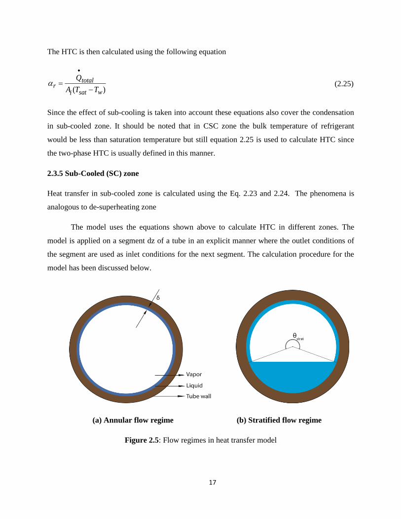
wet the bulk vapor remains at the core of the tube making it annular flow (see Fig. 2.5(a)). The
two-phase HTC in this region is calculated using Cavallini et al. (2006), shown in Eq. (2.16),
where the quality is calculated based on the mass of condensate in the test section. The properties
of liquid and vapor are taken at saturation and superheated conditions respectively.
r i V V
LO r i i
V LVstrat
i sat w
1 33
1.111 3, 7.5 4.3 1 2.6
.5 .1.91
0.8 0.40.023 Pr /
0.253
0.725 1( )
TG l G tt
tt
l l l
l l l
l
J xG gd J X
x v lXx vl
G d d
g h
d T T
LO
A LO V V
TPV
A strat strat
10.3321
1 0.0870.741 1
0.3685 0.23630.8170: 1 1.128
2.144 0.11 Pr
0.8:
TG G l l
l l
T T TG G G G G G
xx
x
J J x
J J J J J J
(2.16)

15
The HTC for sensible heat rejection through superheated vapor is calculated using Eq. (2.13)
with the actual mass flux and properties of superheated vapor. Since, the vapor essentially
remains in the annulus core (see Fig. 2.5); the area for sensible heat rejection can be expressed as
,( 2 )
v Sensible iA d dz (2.17)
Where, δ is calculated using Nusselt theory of film wise condensation
.25[ ( ) / ( ) ]l l sat w lv l l v
T T h g (2.18)
2.3.4 Two-Phase Zone
Two phase zone begins when the bulk temperature of the refrigerant reaches saturation
temperature. Since, the sensible heat rejected by liquid in CSH zone is neglected; the vapor and
liquid will be at saturation temperature at that point. Hence the sensible heat rejected in two
phase zone comes only from liquid.
0,QSensible v (2.19)
The two-phase HTC is again calculated using Eq. (2.14) with calculated quality, actual
properties and mass flux as input. Since Cavallini et al. takes annular and stratified/stratified-
wavy flow regime into account the area of sensible heat rejection is calculated in the following
manner
,
( )
(2 ) ( / )2
i
l sensible istrat
d dz Annular
A dStratified Stratified wavy
(2.20)
Where,
θstrat is calculated using empirical correlation from Thome et al. (2003) (see Fig. 2.5(b)) and
Smith’s correlation (1969) is used to compute void fraction

16
1/33 1/3 1/3(1 ) [1 2(1 ) (1 ) ]22
1 2 2(1 ) [1 2(1 )][1 4(1 ) ]200
strat
(2.21)
1.5/ .4(1 ) /11 .4 .6
1 .4(1 ) /vv l
l
x xx
x x x
(2.22)
The sensible HTC also depends on whether the liquid flow is laminar, turbulent or transition
regime. Hence, Nusselt no. is calculated using constant heat flux, Gnielinski (or Dittus-Boelter)
and Churchill correlations in respective zones.
b i
b i
b
0
4.364 (Re 2300)
8 1000 2, 1.82 log 1.64 (Re 4000)
101 2 2 31 12.7 8 Pr 1
52200 Re
exp136510 10 , (2300 Re 4000)
2 2
.5.079*( / 2) Re Pr
4/5(1 Pr
l
l l lt l l
l
tr lcl
c
Nu
f G d PrNu f G d
f
Nu NuNu Nu
fNu Nu
5/6)
, 6.30
1/5
102 1 Re
2.21ln1/2 710 20(8 / Re) (Re/ 36500)
where Nu
f
Sensible HTC is calculated after finding the Nusselt number for the flow regime of the liquid
Sensible ilNu d (2.24)
(2.23)
17
The HTC is then calculated using the following equation
( )
totalr
wsati
Q
A T T
(2.25)
Since the effect of sub-cooling is taken into account these equations also cover the condensation
in sub-cooled zone. It should be noted that in CSC zone the bulk temperature of refrigerant
would be less than saturation temperature but still equation 2.25 is used to calculate HTC since
the two-phase HTC is usually defined in this manner.
2.3.5 Sub-Cooled (SC) zone
Heat transfer in sub-cooled zone is calculated using the Eq. 2.23 and 2.24. The phenomena is
analogous to de-superheating zone
The model uses the equations shown above to calculate HTC in different zones. The
model is applied on a segment dz of a tube in an explicit manner where the outlet conditions of
the segment are used as inlet conditions for the next segment. The calculation procedure for the
model has been discussed below.
Figure 2.5 (a): Heat transfer model showing annular flow regime
(a) Annular flow regime (b) Stratified flow regime
Figure 2.5: Flow regimes in heat transfer model

18
2.4 Calculation Procedure:
Here is a brief description of the approach taken in the model. The inlet condition of the
refrigerant is superheated vapor such that the wall temperature is greater than saturation
temperature. The HTC on the outer side, tube geometry, inlet mass flux, temperature of air and
refrigerant at inlet are given as input. In order to cover all the zones refrigerant with high
superheat (50-70 0C) at inlet is used as input
For de-superheating zone (DS) use equations 2.9-2.15 to get the HTC using Gnielinski
correlation. Using energy balance approach across each element march down the tube
until wall temperature reaches saturation temperature to enter CSH zone.
CSH zone uses equations 2.9, 2.10, 2.12, 2.13, 2.15-2.18 to get HTC with assumed inlet
quality of .9999 at the beginning. Since condensation begins in this region outlet quality
is calculated in each element and used as input in the next. The vapor temperature is also
calculated and the CSH zone ends where the bulk temperature of vapor reaches saturation
temperature to enter in two-phase zone.
The HTC in CTP and CSC zones are calculated using equations 2.9, 2.10, 2.16, 2.19-2.24
with the inlet conditions to be the output of the last element in CSH zone. The sensible
heat rejected by liquid and hence the temperature of bulk liquid is calculated to quantify
the sub-cooling of liquid at the end of two-phase zone. The bulk enthalpy and
temperature of refrigerant is computed separately and the two-phase zone ends when the
bulk temperature of refrigerant drops below saturation temperature.
Once the refrigerant enters sub-cooled (SC) zone, equations 2.23 and 2.24 are used to
calculate HTC in each element.
The model described above is able to eliminate the discontinuity across various zones in the
condensation process. The preliminary results from the model and their comparison to
experimental data has been shown and analyzed in details in the next section.

19
CHAPTER 3
EXPERIMENTAL METHOD
3.1 Facility for Experiments
Figure 3.1 shows the schematic diagram of experimental apparatus. The refrigerant loop
mainly consists of a variable speed gear pump, a coriolis-type mass flow meter, an electric pre-
heater, a mixer, a pre-cooler, a test section, sight glass, two after-coolers and receiver tank. The
refrigerant flow rate is regulated by the gear pump while the pressure is controlled by the
refrigerant charge amount, pre-heater and flow rate of water through the after-coolers. The inlet
condition at test section is adjusted by water flow rate through pre-cooler while the heat flux is
controlled by the mass flow rate and inlet/outlet temperature of the cooling water in test section.
The state of the refrigerant can be seen in the sight glass downstream of the test section. The
cooling water in the pre-cooler and test section is again cooled in a separate loop with chilled
water supply line.
Figure 3.1: Schematic diagram of the experimental apparatus

20
3.2 Test Section
Figure 3.2 (a) and (b) show the schematic of the test section and arrangement of
thermocouples on the test tube. The test section consists of a smooth copper tube with 6.1 mm ID
and 9.53 mm OD and 150 mm length. The tube is placed horizontally and covered with a thick
brass jacket which ensures uniform cooling throughout the test section. The halved brass jacket
is pressed over the test tube and the small gap between them is filled with a thermal paste. The
cooling water flows through copper tubes soldered to the outer surface of the brass jacket.
Twelve thermocouples are embedded into the top, bottom, right, and left of the test tube wall at
three positions in the axial direction. The short length of test section allows us to measure the
quasi-local HTC with relatively accurate test conditions.
(a) Test Section (b) Dimensions of the test tube
Figure 3.2: Specifications of the test section and test tube.
3.3 Experimental Measurement and Uncertainties
During experiments the refrigerant is ensured to be in superheated state in the pre heater
with a superheat of 5-50 0C. The pre cooler is in operation even for readings in superheated state.
The enthalpy in pre heater is calculated by measured pressure and temperature. The inlet
condition of test section is then achieved by controlling the heat rejection from pre cooler which
is a function of measured mass flow rate and ∆T of cooling water. The T type thermocouples
measure the wall temperature and heat flux is calculated using mass flow rate, inlet and outlet
1mm
2mm
6.1 mm ID
9.53 mm OD
Thermocouple
Tin

21
temperature of cooling water through test section. The pressure drop in the test section and pre
cooler is again measured by a differential transducer which gives the precise pressure in test
section. The uncertainties of the instruments used in the experiments have been given in Table
3.1. The uncertainty propagation (Moffat, 1988) because of the instruments is shown in the form
of error bars in the data shown below.
Table 3.1: Measurement uncertainties
Nomenclature Instrument Uncertainty
Trb, TH2O Sheathed T type Thermocouple ±0.05 K
Twi Twisted T type Thermocouple ±0.16 K
PMC Diaphragm absolute pressure
transducer ±4 kPa
PDiaphragm differential
pressure transducer ±0.13 kPa
H2O, TS,m rm Coriolis mass flow meter ±0.1 g/s
H2O, PCm Coriolis mass flow meter ±0.5 g/s
3.4 Range of Test Conditions
The experiments have been conducted for 3 refrigerants viz. R1234ze(E), R134a and R32 for the
range of operating conditions illustrated in Table 3.2. The operating conditions have been chosen
to be close to condenser pressure in automotive systems. The wide range of experiments
conducted allows making a comparison between the refrigerants and analyzing the effect of
various parameters on HTC.
Table 3.2: Test Range for the experiments
Refrigerant G
[kgm-2
s-1
]
Tsat
[0C]
Q
[kWm-2
]
R1234ze(E) 100-300 30-50 5-25
R134a 100,300 30,50 10
R32 100,300 30,50 10

22
3.5 Data Reduction Procedure
Figure 3.3 helps presenting the data reduction method. The main measured values are the
refrigerant mass flow rate ṁr, bulk-mean temperature Trb,MC, and absolute pressure PMC in the
mixer, the bulk water temperature of pre-cooler inlet TH2O,PCi and outlet TH2O,PCo, test section inlet
TH2O,TSi and outlet TH2O,TSo, and the water mass flow rate of pre-cooler ṁH2O, PC and test section
ṁH2O, TS. The bulk-mean enthalpy in the mixer hrb,MC is obtained from Trb,MC and PMC under the
assumption of equilibrium by RefpropVer.8.0 (Lemmon et al., 2007). The enthalpy changes
through the pre-cooler ∆hPC and the test section ∆hTS are determined by water side heat balances
and as presented below.
rPC H2O,PCo H2O,PC H2OH2O,PCi gain,PCh T T m Cp Q m
(3.1)
rTS H2O,TSo H2O,TS H2OH2O,TSi gain,TSh T T m Cp Q m
(3.2)
Where gain,PC and gain,TS are preliminarily measured heat leak from ambient air through the
insulators. The bulk mean temperature at the test section Trb is obtained from bulk enthalpy and
pressure with the equilibrium state function of RefpropVer.8.0.
rb rb,i rb,o
PC MC PCrb,i b,MC
PC TS MC PC TSrb,o b,MC
2
,
,
equiblium
equiblium
T T T
T f h h P P
T f h h h P P P
(3.3)
The average heat flux of the test section on the interior tube wall qwi is,
H2O,TSo H2O,TS H2OH2O,TSi gain,TS cond
wii
T T m Cp Q Qq
d Z
(3.4)
Where, Qcond is the conduction heat from outside the cooling brass jacket estimated
numerically for each condition. The definition of average heat transfer coefficient α is,
wi rb wi,q T T T T (3.5)

23
MCPTSoPTSiP
rb,MCT
b,MChb,ihb,oh
PCP
TS TS r/h Q m
rb,iTrb,oT
T
T
TT
P
PC PC r/h Q m
TSP
Pre-coolerTest section
※Circled values are measured.
T
Mixer
P
Test tube
(12 points)T
25mm150mm
50mm50mm
288mm
Always superheated(SH 5K~)
Pre-heater
Where, Twi is the average temperature of the 12 points on the tube wall. The reference
refrigerant temperature is defined as an arithmetic mean of inlet and outlet bulk temperatures Trb,i
Trb,o, which are found from each pressure PTSi and PTSo and enthalpies hb,i and hb,o. With this
method, driving temperature difference ∆T in superheat zone is defined as the difference between
tube wall and bulk refrigerant temperature. Then this continuously changes into the difference
between tube wall and saturation temperature at the thermodynamic vapor quality 1.0 for two-
phase zone. Table 3.1 lists the measurement uncertainties obtained from the results of two
standards deviation of calibration, resolution of data loggers and calibration tools, and the
stability of excitation voltages. Combined measured uncertainties are calculated from those
uncertainties in conformity of ASME Performance Test Codes, 1985 and Moffat (1988).
Figure 3.3: Data reduction procedure.

24
CHAPTER 4
RESULTS AND DISCUSSION
4.1 Smooth Transition of HTC across Superheated, Two Phase and Sub-
Cooled Zone
Figure 4.1 shows the experimental results for heat transfer coefficient for three
refrigerants: R1234ze (E), R134a and R32. It can be seen that all the three refrigerants exhibit
similar pattern in condensation showing smooth transition from de-superheating to two-phase
and two-phase to sub-cooled zone respectively. Figure 4(a) shows heat transfer data for
R1234ze(E) at 100 kgm-2
s-1
, 10 kWm-2
and saturation temperature of 500
C which is typical
operating conditions for this refrigerant. Figures 4(b) and 4(c) are the results for R134a and R32
at same operating conditions to generalize the results. The horizontal axis indicates bulk mean
enthalpy of refrigerant in the test section while the vertical lines mark the saturation conditions at
that condition. The enthalpy of refrigerant has been calculated under the assumption of
equilibrium even during condensation in superheated zone. The upper graph shows the variation
of HTC with the inlet condition in the test section. The uncertainty of the experimental
measurements has been shown through error bars where the horizontal and vertical bars
represent uncertainty in enthalpy and HTC respectively. The experimental data has been
compared with the model developed with single phase Gnielinski correlations in de-superheating
and sub-cooled zones. The heat transfer coefficient is seen to be in satisfactory agreement with
the model. Since the model is developed for a flow with superheated inlet it is difficult to
replicate the exact experimental conditions which were induced artificially. The center graph
shows the bulk mean inlet (Trb,i), outlet (Trb,o) and wall temperature (Twi) in the test section. It
should be noted that the inlet and outlet temperatures are fairly close to each other on account of
short test section length. The bottom graph shows the temperature difference between bulk
refrigerant and wall which is represented by (Trb,i+Trb,o)/2 – Twi. It can be seen through the center
figures that wall temperature is the major driving force in the transition from superheat to
condensing superheat zone. The HTC in the top figure starts deviating from Gnielinski
correlation when the wall temperature drops below saturation temperature indicating the start of
condensation. Also, the HTC in the sub-cooled zone is much higher than single phase prediction

25
near x=0. This is due to the presence of vapor in the sub-cooled region on account of sub-cooled
liquid film. Condensation in superheated, two phase and sub-cooled region has been explained in
detail in later sections.
Figure 4.1: Comparison between experimental results and prediction by proposed model

26
4.1.1 Condensation in Superheated Zone
Figure 4.2 shows the variation of HTC in CSH zone where the vertical axis crosses horizontal
axis at saturation vapor enthalpy of the refrigerant. The HTC starts deviating from single phase
correlation when wall temperature reaches saturation temperature and increases until bulk
refrigerant reaches saturation temperature. The increase is HTC can be attributed to increased
heat rejection due to condensation. As shown in the top graph of Fig. 4.2, the component of heat
transfer due to condensation increases downstream and eventually contributes to the majority of
heat transfer near x=1. The presence of condensation is corroborated with increasing film
thickness inside the tube. The model predicts the HTC in CSH zone within accuracy of 14.5 %.
4.1.2 Condensation in Two Phase Zone
Figure 4.3 shows the variation of HTC in TP zone where the ends of horizontal axis are marked
by the saturation enthalpy of the refrigerant. The sensible heat rejected by the liquid film is
negligible at the beginning but contributes approximately 15% of the total heat rejection at the
end of two phase zone. As a result the liquid temperature also decreases sharply near x=0. The
sub-cooling of liquid film results in the presence of vapor when the bulk enthalpy of refrigerant
reaches saturation enthalpy. This leads us to the conclusion that condensation will occur even in
the sub-cooled zone. The HTC in this zone is predicted within accuracy of 14.8 %.
4.1.3 Condensation in Sub-Cooled Zone
As shown in Fig. 4.4 HTC in condensing sub-cooled zone is higher than prediction by single
phase correlations due to presence of vapor at the end of two phase zone. HTC decreases in CSC
zone as the sensible heat rejection starts dominating two phase heat transfer. The bulk refrigerant
and liquid film temperature converges at the end of this zone marking the beginning of sub-
cooled zone. The jump in the model can be explained to be a result of simplified calculations for
heat transfer through liquid film as only annular and stratified flow regimes are taken into
account in the model. The sudden decrease in HTC occurs when the last existing vapor
condenses in the element eliminating two phase heat transfer entirely. The HTC in CSC zone is
not predicted extremely well by the model (accuracy of 24.8%) and the authors are working on
visualization in condensers to address this issue.

27
Figure 4.2: Prediction vs. results for heat rejection in superheated zone
R1234ze(E) at G= 100kgm-2
s-1
, Tsat = 50 0C, Q= 10 kWm
-2

28
Figure 4.3: Prediction vs. results for heat rejection in two phase zone
R1234ze(E) at G= 100kgm-2
s-1
, Tsat = 50 0C, Q= 10 kWm
-2

29
Figure 4.4: Prediction vs. results for heat rejection in sub-cooled zone
R1234ze(E) at G= 100kgm-2
s-1
, Tsat = 50 0C, Q= 10 kWm
-2

30
4.2 Effect of Parameters on Heat Transfer Coefficient
The HTC for three refrigerants have been determined under various operating conditions
to have a reasonable comparison of the refrigerants and also form a conclusion regarding the
effect of various parameters on HTC.
4.2.1 Effect of Mass Flux
The effect of mass flux on HTC can be seen through Figure 4.5 for R1234ze(E). The
HTC decreases with vapor quality in the two-phase region. This is due to the fact that as vapor
quality decreases the velocity of vapor decreases significantly to maintain the same mass flux
and increased presence of liquid increases thermal resistance. This results in a less turbulent flow
which decreases the HTC. Similarly, with decrease in mass flux the refrigerant moves with a
lower velocity which reduces the HTC on the refrigerant side.
Figure 4.5: Effect of mass flux on HTC for R1234ze(E) at Tsat = 50 0C, Q = 10 kWm
-2

31
The effect of mass flux, however, diminishes at low qualities as higher mass flux results
in greater film thickness at wall increasing the resistance from liquid. Thus the effect of high
vapor velocity is diminished by greater film thickness. It can be seen that Cavallini and Kondo-
Hrnjak correlations captures the effect of mass flux on HTC fairly well. The increase in
experimental deviation from correlations at very high qualities can be a result of presence of mist
flow regime which is not taken into account in the Cavallini correlation. Mist flow would allow
liquid entrainment into vapor core which reduces film thickness resulting in higher HTC.
4.2.2 Effect of Heat Flux
Figure 4.6 shows the HTC of R1234ze(E) at 100kgm-2
s-1
, 30 0C saturation temperature at various
heat fluxes. It has been observed that the HTC in two phase zone increases slightly when the heat
flux is increased from 5 to 10 kWm-2
but it remains constant from 10 to 25 kWm-2
. Nusselt
condensation theory, which is used in most correlations, suggests that HTC should decrease with
increase in heat flux on account of larger film thickness which increases resistance on the
refrigerant side. This theory, however, was proposed for laminar free convection condensation
assuming quiescent vapor ignoring the effect of forced convection of the vapor. Experimental
data shows that the effect of heat flux is limited and similar trend was observed for condensation
of CO2 in smooth tubes (Kondou and Hrnjak, 2012). Since the tube wall temperature decreases
as heat flux increases condensation is seen to begin at higher bulk temperatures for higher heat
flux operating conditions.
4.2.3 Effect of Saturation Temperature
Figure 4.7 shows the comparison of HTC for R1234ze(E) at saturation temperature of 30, 40 and
50 0C. The effect of saturation temperature is not as significant as mass flux as the HTC
increases/decreases due to change in thermo physical properties of the refrigerant which do not
vary drastically in these operating conditions. However, as pressure increases the vapor density
of refrigerant increases lowering the vapor velocity. Also, the decrease in liquid thermal
conductivity, Pr and latent heat increases the resistance in the refrigerant side. The combined
effect of these thermo-physical properties reduces the HTC with increase in pressure. It is also to
be noted that the HTC is well predicted by Cavallini correlation at saturation temperature of
500C but the correlation starts to deviate at lower saturation conditions.

32
Figure 4.6: Effect of heat flux on HTC for R1234ze(E) at G= 100 kgm-2
s-1
and Tsat = 30 0C
Figure 4.7: Effect of Tsat on HTC for R1234ze(E) at G=100 kgm-2
s-1
, Q=10 kWm-2

33
4.3 Comparison of HTC for Different Refrigerants
R1234ze(E) is currently considered to be a potential replacement for R134a due to its
similar thermo physical properties and low GWP and especially in mixtures with R32 that would
bring it even closer to be almost drop in replacement. The heat transfer performance for
R1234ze(E), however, has not been widely established yet. Hence, a comparative study between
the two refrigerants has been done to establish a baseline. It has been known that R32 has
favorable thermo physical properties like high latent heat, high liquid thermal conductivity for
heat transfer in condensation. Therefore one of the potential methods to improve the performance
of automotive systems is to replace R134a with a mixture of R1234ze(E) and R32. The
experimental data in this paper can be used as a comparison for R1234ze(E) and R32 mixture to
ascertain the degradation in HTC.
4.3.1 Heat Transfer Coefficient
Figure 4.8 shows the HTC and pressure drop for the three refrigerants at same operating
conditions. The HTC of R134a is slightly higher than R1234ze(E). The refrigerants do not show
much variation owing to similar thermo physical properties which determines HTC. The
properties of R32, however, are better suited for condensation process due to higher latent heat,
Pr and liquid thermal conductivity as shown in Table 4.1. As a result, R32 displays much higher
HTC compared to R1234ze(E) and R134a. Thus a mixture of R32 and R1234ze(E) is a potential
option to improve the performance in automotive and stationary systems. The HTC has been
well predicted by Cavallini correlation in all three cases.
4.3.2 Pressure Drop
The pressure drop gradient for R1234ze(E) is seen to be significantly higher than R134a from
Figure 4.8. The lower vapor density of R1234ze(E) results in higher velocity at same mass flux
as R134a. This results in a higher slip at liquid vapor interface increasing frictional pressure
drop. High vapor density of R32 results in a much lower pressure drop compared to R134a and
R1234ze(E). The pressure drop data is in good agreement with Friedel (Friedel, 1979)
correlation in two phase region. However, pressure drop in superheated region decreases with

34
increase in enthalpy indicating that condensation in superheated region effects pressure drop and
a new model needs to be developed for pressure drop in CSH zone.
Thus, R32, with higher HTC and lower pressure drop gradient potentially has the benefits of
being used as a component in a mixture. The flammability of the refrigerant, however, may still
pose a problem.
Figure 4.8: HTC and Pressure drop comparison between R1234ze(E), R134a and R32 at G=100
kgm-2
s-1
, Tsat = 500C, Q=10 kWm
-2
Table 4.1: Thermo physical properties of refrigerants of interest
Tsat = 400C
Psat
(MPa)
ρl
(kg/m3)
ρv
(kg/m3)
hlv
(kJ/kg)
λl
mW/(m.K)
Cpl
kJ/(kg.K)
µl
(µPa s)
Prl
σl
(mN/m)
GWP
R1234ze(E) 0.77 111.3 40.7 154.6 69.3 1.4 167 3.48 6.96 6
R134a 1.016 1146.7 50.1 163.1 74.7 1.5 161.5 3.24 6.12 1300
R32 2.49 893.4 73.3 237.1 114.6 2.16 95 1.79 4.47 550

35
4.4 Comparison of Experimental Data to Prediction
The experimental data obtained in the study has been compared to well known
correlations and the proposed model. Since the correlations available in literature are proposed
for two phase flows, Kondo-Hrnjak correlation is combined with two-phase correlations to
predict data set in condensing superheat zone and the data in the sub-cooled region is not taken
into account. However, the proposed model takes into account all the data points and thus gives
good overall prediction accuracy.
4.4.1 Comparison to Correlations from Literature
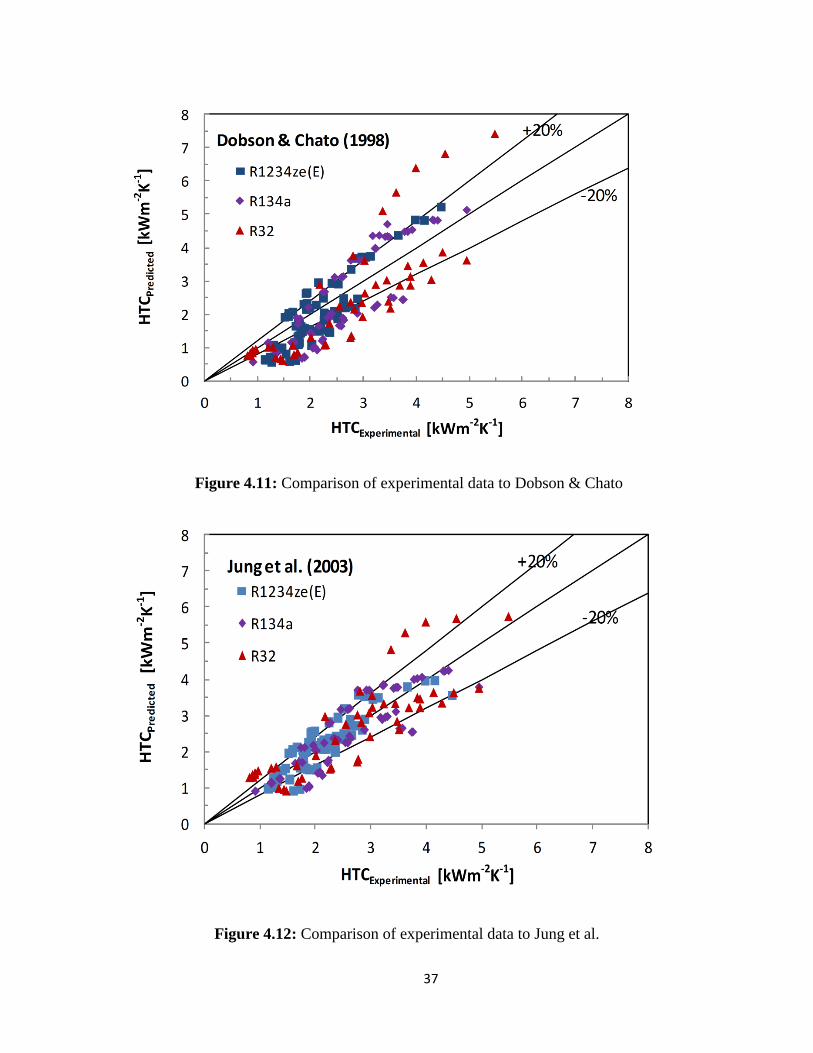
The HTC from the experiments have been compared to well-known correlations by
Cavallini et al. (2006), Thome et al. (2003), Jung et al. (2003), Dobson & Chato (1998) and
Haraguchi et al. (1994). Table 4.2 lists the deviation of correlations from experimental data.
Since the correlations mentioned above were developed for two phase flows the condensation in
CSH zone is predicted with Kondo-Hrnjak correlation which is a function of selected two-phase
correlation.
Figure 4.9 to 4.13 compares predicted results with experimental data for all five
correlations. Correlations of Cavallini and Thome predicted the data with mean deviation of
12.1% and 10.5% respectively. It is noted that correlation by Cavallini et al. (2006) doesn’t
capture HTC at high qualities well as it takes only annular flow regime into account at high
qualities. The film thickness at high qualities could be less than assumed in annular flow which
would lead to under prediction of HTC. The correlation proposed by Thome et al. (2003) is
based on flow regime map and it seems to capture HTC at high qualities fairly well. Dobson and
Chato (1998) developed the correlation with the assumption that ratio of HTC in single and two-
phase is a function of Martinelli’s parameter. Since the effect of mass flux and latent heat were
not taken into account, the correlation predicted the data with a deviation of 27.2%. Jung et al.
considered the effect of these parameters and modified Dobson and Chato correlation by
including heat to mass flux ratio in the correlation which predicted experimental data slightly
better with 17% deviation. Haraguchi et al. (1994) predicted data for R1234ze(E) and R134a
reasonably well but failed to capture data for R32.

36
Figure 4.9: Comparison of experimental data to Cavallini et al.
Figure 4.10: Comparison of experimental data to Thome et al.
37
Figure 4.11: Comparison of experimental data to Dobson & Chato
Figure 4.12: Comparison of experimental data to Jung et al.

38
Figure 4.13: Comparison of experimental data to Haraguchi et al.
4.4.2 Comparison to the Proposed Model
The model has been compared to experimental data for R1234ze(E), R134a and R32 for
condensation in superheated, two phase and sub-cooled region. Table 4.3 shows the deviation of
experimental HTC from the model for 3 refrigerants. The prediction for condensation in
superheated and two-phase regions is reasonably accurate. However, the model does not predict
the HTC in sub-cooled region with great accuracy. This could be attributed to the fact that the
sub-cooling accounted in the model is based only on flow regimes of annular and
stratified/stratified wavy flows. The area associated with sub-cooling is not entirely accurate as it
does not take the transition from annular to slug/plug flows into account. Hence, the simplistic
approach for sub-cooling calculations leads to deviation of model from experimental data.
Overall deviation of experimental data from the model has also been shown in figure 4.14. From
figure 4.15 is seen that the model accurately predicts the transition point for CSH zone which
strengthens the argument of wall temperature being the driving force behind the start of
condensation. Also the summary of experimental results indicates that the model works well for
different refrigerant at different operating conditions with accurate prediction of local HTC.

39
Table 4.2: Mean Absolute Deviation of various correlations against experimental data
Refrigerant
Cavallini/Kondo-
Hrnjak
Thome/Kondo-
Hrnjak
Jung/Kondo-
Hrnjak
Dobson &
Chato/Kondo-
Hrnjak
Haraguchi/Kondo-
Hrnjak
Two
phase
(%)
CSH
(%)
Two
phase
(%)
CSH
(%)
Two
phase
(%)
CSH
(%)
Two
phase
(%)
CSH
(%)
Two
phase
(%)
CSH
(%)
R1234ze(E) 12 28 10 25 14 22 25 26 20 40
R134a 11 24 8 22 15 19 27 28 19 42
R32 14 16 15 28 25 19 30 16 42 24
Overall 12.1 22.8 10.5 24.8 16.9 20 27.2 23.7 25 36.2
Table 4.3: Mean Absolute Deviation of proposed model against experimental data
Refrigerant Condensation Zone
Overall Superheated Two-phase Sub-cooled
R1234ze(E) 12.9 14.5 26.6 15.7
R134a 17.6 13.9 19.3 16.3
R32 13.2 15.8 27.1 15.5
Overall 14.5 14.6 24.8 15.8

40
Figure 4.14: Comparison of experimental HTC with proposed model

41
Figure 4.15: Summary of experimental data and comparison with proposed model

42
4.5 Summary of Experimental Results
Figure 4.18 to 4.20 shows experimental and predicted HTC of the three refrigerants
where the lines show the prediction by Cavallini and Kondo-Hrnjak correlation in two-phase and
superheated condensing zone respectively. The predicted HTC agrees with experimental data for
all the refrigerants at given conditions.
The HTC has been plotted in P-h diagram to gain a better understanding of the
condensation process in condensers at various pressures and analyze the importance of
condensing superheated zone. As the latent heat of the refrigerant reduces with increase in
pressure the capacity of condensers is more affected by heat transfer in condensing superheated
zone. This becomes extremely important for refrigerants operating near critical point where
latent heat is very small. The effect has been quantified with CO2 by Kondo & Hrnjak (2012)
Figure 4.16: Variation of HTC with pressure and enthalpy for R1234ze(E)

43
Figure 4.17: Variation of HTC with pressure and enthalpy for R134a
Figure 4.18: Variation of HTC with pressure and enthalpy for R32

44
CHAPTER 5
SUMMARY, CONCLUSIONS & RECOMMENDATIONS
5.1 Summary and Concluding Remarks
A new heat transfer model based on the principle of energy conservation in horizontal
tubes has been proposed which asymptotically satisfies the single phase correlations by taking
the sensible heat rejection in condensation into account. The presence of liquid in de-
superheating region accounts for the discontinuity in condensing superheated zone while the
presence of vapor in sub-cooled region has been seen to effect the heat transfer coefficient near
x=0. Liquid sub-cooling in two-phase region is quantified which explains the smooth transition
from two-phase to sub-cooled zone. Thus the model eliminates the discontinuity at very high and
low qualities predicting experimental data within 16% accuracy. The model includes well known
correlations of Cavallini and Gnielinski taking flow regime into consideration. This is the first
attempt to include and quantify the effect of sensible heat in two phase zone and the model can
be improved by taking a more detailed approach in terms of flow regime and other two-phase
correlations available in literature.
The results from the model have been validated by experiments conducted with different
refrigerants at various operating conditions. Experiments have been conducted for R134a,
R1234ze(E) and R32 for mass fluxes of 100-300 kgm-2
s-1
, saturation temperatures of 300 C-50
0 C
and from sub-cooling of 20 0C to superheat of 50
0C in a horizontal smooth tube with 6.1 mm
inner diameter. The beginning of condensation in superheated zone has been proved to be the
criteria Twall<Tsat by observing the wall temperature and deviation of experimental HTC from
single phase correlations simultaneously. It has also been shown through experiments that HTC
in sub-cooled region is much higher than single phase predictions due to presence of vapor as
seen in the sight glass located at the end of the test section. The effect of various parameters on
HTC has been quantified and analyzed to present a thorough study of condensation process. The
results are also compared to well known correlations available in literature with satisfactory
agreement.

45
The following points are considered to be the most important takeaways from the work
presented:
Condensation in a tube occurs not only in two phase zone but also in superheated and
sub-cooled zone due to presence of liquid and vapor respectively.
The transition from superheated to condensing superheated zone is seen when the wall
temperature drops below saturation temperature of refrigerant where the HTC starts
deviating from the Gnielinski correlation and approaches the HTC at x=1.
HTC is seen to be significantly greater than single phase predictions near x=0 in sub-
cooled zone due to presence of saturated vapor with sub-cooled liquid film.
The model proposed in this work successfully takes into account the effect of sensible
heat rejection in condensation providing a better physical explanation of the process. The
model is validated by the experimental results to be within 16 % accurate.
HTC increases significantly with mass flux, decreases slightly with increase in saturation
temperature and practically not affected by heat flux. Among the correlations available in
literature HTC is fairly well predicted by Thome/Cavallini and Kondo-Hrnjak
correlations in two-phase and superheated-condensation zone respectively.
Pressure drop is well captured by Friedel correlation for all the refrigerants at various
operating conditions in the two phase zones and experiments suggests that pressure drop
is affected due to the presence of liquid film in CSH zone.
R1234ze(E) has very similar heat transfer characteristics as R134a due to close thermo-
physical properties. However, R1234ze(E) exhibits much higher pressure drop which
should be considered while using it as a drop-in replacement.
R32 has higher HTC and lower pressure drop than R1234ze(E) and R134a and hence is a
feasible option to be considered as a mixture component to improve the heat transfer
performance in automotive systems.

46
5.2 Recommendations for Future Study
The work presented in the thesis is an attempt to explain the process of condensation
from de-superheating to sub-cooled zone from a physical point of view. The assumptions taken
in the model like heat leak, uniform properties on the perimeter of tube can be refined to give
more accurate results. Although the model proposed is based on first principle it still is
dependent on the correlations proposed for two phase zones. The future work of this study is to
conduct experiments with flow visualization which will give a better explanation of the flow
regimes and the process of condensation in the transition zones. The sight glass installed in this
study at the end of test section was not appropriate for visualization. Hence, a transparent tube
downstream of test section will be installed and experiments can also be conducted with the test
in the transparent section itself. One of the objectives to perform this test is to measure film
thickness in the test section. From a practical point of view the thickness of liquid film is the key
to find the exact proportion of sensible and latent heat rejection in the process. Once, the film
thickness is known more physical models can be proposed for condensation in superheated zone.
It has been pointed out throughout this work that R32 can be used as a component in a
mixture with R1234ze(E) to be used as a replacement in automotive systems. The experimental
data taken in the thesis can be used as a baseline to analyze the effect of mixtures on HTC. Since,
experiments have been conducted with R1234ze(E), R134a and R32 it would be facilitate
comparison of HTC of mixtures with individual component and R134a. Previous studies with
zeotropic mixtures which indicates that the concentration of individual component have a huge
impact on the degradation of HTC in mixtures. The temperature glide of mixture which is also a
function of concentration ratio affects the HTC as well. Hence effort should be made to find the
ideal concentration ratio of R1234ze(E) and R32 which can show similar heat transfer
performance as R134a. The concentration ratio, however, depends on various other factors viz.
flammability, GWP etc. and caution should be taken to select a mixture with realistic
concentrations acceptable in industries.

47
APPENDIX A
CALIBRATION RESULTS
A.1 Thermocouple Calibration
Table A.1: Thermocouples electro motive force at different temperatures (unit: 0C, mV)
Temp 21.065 14.420 13.690 20.095 30.895 30.915 43.072 33.980 34.000
1T 0.840 0.579 0.546 0.797 1.234 1.232 1.722 1.355 1.354
1R 0.841 0.580 0.547 0.798 1.234 1.232 1.722 1.356 1.355
1B 0.840 0.579 0.547 0.797 1.232 1.231 1.720 1.354 1.353
1L 0.840 0.580 0.547 0.798 1.233 1.231 1.719 1.353 1.352
2T 0.840 0.578 0.546 0.796 1.234 1.232 1.722 1.354 1.353
2R 0.842 0.580 0.547 0.798 1.235 1.233 1.719 1.354 1.351
2B 0.840 0.579 0.546 0.797 1.234 1.232 1.722 1.355 1.354
2L 0.841 0.580 0.546 0.796 1.233 1.231 1.721 1.355 1.354
3T 0.840 0.579 0.547 0.798 1.234 1.233 1.720 1.340 1.341
3R 0.837 0.579 0.546 0.796 1.232 1.230 1.720 1.354 1.353
3B 0.841 0.580 0.547 0.798 1.234 1.232 1.722 1.356 1.355
3L 0.840 0.579 0.546 0.797 1.232 1.230 1.720 1.354 1.353
Temp 22.177 22.152 16.197 38.190 44.802 44.845 49.755 49.762 55.470
1T 0.890 0.887 0.647 1.518 1.787 1.786 1.989 1.991 2.234
1R 0.891 0.888 0.649 1.519 1.787 1.789 1.989 1.991 2.234
1B 0.890 0.888 0.647 1.517 1.785 1.787 1.987 1.990 2.232
1L 0.890 0.888 0.648 1.516 1.784 1.786 1.985 1.986 2.231
2T 0.888 0.886 0.645 1.519 1.789 1.792 1.993 1.995 2.235
2R 0.887 0.891 0.643 1.521 1.792 1.793 1.996 1.998 2.238
2B 0.890 0.888 0.647 1.520 1.790 1.791 1.993 1.995 2.235
2L 0.892 0.890 0.648 1.517 1.786 1.788 1.989 1.991 2.230
3T 0.872 0.876 0.634 1.520 1.791 1.793 1.996 1.998 2.236
3R 0.890 0.888 0.648 -1.552 -5.679 -5.695 -6.448 -5.240 -5.121
3B 0.890 0.889 0.649 1.518 1.790 1.792 1.995 1.997 2.235
3L 0.892 0.888 0.648 1.516 1.788 1.789 1.992 1.994 2.231

48
Temp 55.97 62.137 62.082 42.805 37.935 26.830 36.900 36.920 42.165
1T 2.252 2.525 2.523 1.711 1.513 1.069 1.464 1.467 1.678
1R 2.251 2.523 2.522 1.710 1.510 1.069 1.463 1.466 1.677
1B 2.250 2.523 2.522 1.709 1.509 1.066 1.461 1.464 1.677
1L 2.248 2.521 2.520 1.708 1.508 1.067 1.462 1.465 1.677
2T 2.253 2.526 2.525 1.711 1.509 1.066 1.463 1.467 1.678
2R 2.256 2.529 2.528 1.707 1.503 1.068 1.465 1.468 1.680
2B 2.253 2.527 2.525 1.711 1.510 1.066 1.463 1.466 1.679
2L 2.248 2.521 2.521 1.711 1.510 1.066 1.461 1.464 1.675
3T 2.253 2.527 2.525 1.704 1.507 1.066 1.465 1.468 1.680
3R -4.88 -4.797 -4.907 1.708 1.509 1.065 1.461 1.464 1.676
3B 2.252 2.525 2.524 1.711 1.511 1.064 1.463 1.466 1.678
3L 2.248 2.521 2.520 1.709 1.509 1.063 1.461 1.465 1.676
Table A.2: Calibration results
a3 a2 a1 a0 2σ
1T -0.52125 1.71077 23.43247 0.44586 0.149
1R -0.49007 1.56250 23.67289 0.31250 0.149
1B -0.49586 1.55819 23.72615 0.30389 0.150
1L -0.53664 1.74846 23.49660 0.37002 0.142
2T -0.40298 1.16498 24.14053 0.20820 0.141
2R -0.42176 1.20013 24.15775 0.15666 0.159
2B -0.42499 1.25572 24.04528 0.21288 0.149
2L -0.48931 1.56131 23.68766 0.31551 0.184
3T -0.17860 0.11364 25.54355 -0.23631 0.226
3R -0.89902 2.84900 22.41952 0.72722 0.180
3B -0.35502 0.92952 24.52264 -0.00702 0.167
3L -0.38174 1.06129 24.36817 0.06421 0.176
Standard deviation: 2σ= 0.16 [K], T = a3 E 3+ a2 E
2 + a1 E + a0 [
oC] E [mV]
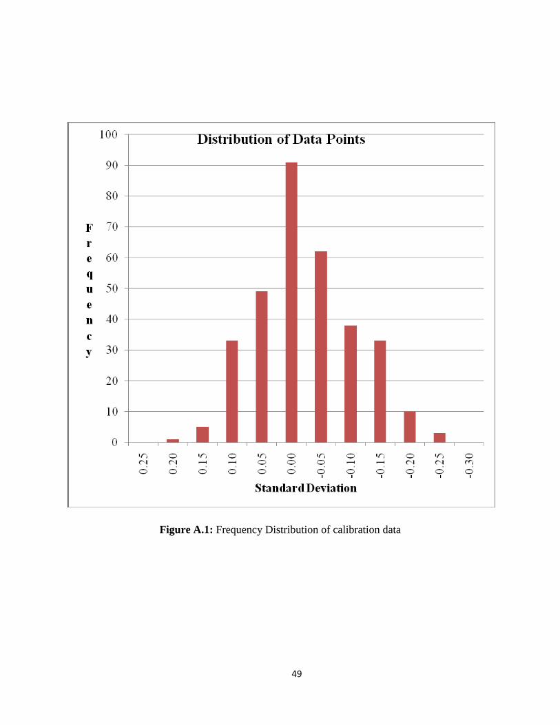
49
Figure A.1: Frequency Distribution of calibration data

50
Table A.3: Verification of Thermocouple calibration using Precision Thermocouple
Precision Thermocouple 1 Thermocouple 2 Precision Thermocouple 1 Thermocouple 2
[0C] [
0C] [
0C] [
0C] [
0C] [
0C]
10.274 10.2 10.23 30.213 30.01 30.16
10.277 10.2 10.25 30.218 30.01 30.16
10.283 10.2 10.28 30.213 30.08 30.18
10.278 10.13 10.23 30.216 30.03 30.16
10.275 10.18 10.25 30.213 30.03 30.18
10.278 10.1 10.23 30.215 30.03 30.16
10.278 10.18 10.23 30.214 30.03 30.13
10.28 10.18 10.23 30.213 30.01 30.16
10.277 10.18 10.23 30.215 30.01 30.13
10.276 10.2 10.23 30.212 30.01 30.13
10.276 10.18 10.17 30.214 30.03 30.16
10.28 10.18 10.23 30.212 30.03 30.16
10.281 10.23 10.23 30.215 30.03 30.16
10.281 10.18 10.17 30.212 30.01 30.16
10.282 10.18 10.23 30.215 30.01 30.13
20.249 20.13 20.16 40.18 40.01 40.13
20.252 20.15 20.16 40.18 40.01 40.1
20.251 20.1 20.16 40.176 39.99 40.1
20.253 20.13 20.16 40.178 40.01 40.1
20.252 20.13 20.16 40.177 39.94 40.06
20.252 20.13 20.16 40.179 39.94 40.08
20.255 20.1 20.16 40.18 40.01 40.1
20.249 20.1 20.16 40.181 39.99 40.1
20.251 20.1 20.16 40.181 39.99 40.18
20.25 20.13 20.21 40.181 39.94 40.1
20.252 20.13 20.16 40.18 39.99 40.18
20.248 20.13 20.16 40.181 39.92 40.13
20.251 20.13 20.16 50.146 49.9 50.04
20.249 20.13 20.21 50.147 49.9 50.09
20.251 20.1 20.16 50.148 49.9 50.02
50.15 49.9 50.07 50.149 49.9 50.07
50.145 49.95 50.07 50.138 49.95 50.07
50.147 49.88 50.07 50.142 49.97 50.07
50.144 49.95 50.02 50.144 49.95 50.07
50.149 49.9 50.09 50.14 49.95 50.07

51
A.2 Pressure Transducer Calibration
Table A.4: Pressure Calibration Readings
Pressure [kPa] Voltage [V]
99.898 0.021
442.898 0.144
700.898 0.237
997.398 0.343
1288.898 0.449
1604.898 0.564
1897.898 0.67
2212.898 0.785
2424.898 0.862
Figure A.2: Calibration of Absolute Pressure Transducer
y = 2763x + 45.684
0
500
1000
1500
2000
2500
3000
0 0.2 0.4 0.6 0.8 1
Pre
ssu
re [
kP
a]
Voltage [V]

52
Table A.5: Pressure Calibration Data
Voltage
[V]
Pressure
[Kpa]
Voltage
[V]
Pressure
[kPa]
Voltage
[V]
Pressure
[kPa]
Voltage
[V]
Pressure
[kPa]
Voltage
[V]
Pressure
[kPa]
0.151 100.3 0.474 318.8 0.967 659 1.298 885.6 1.646 1127.6
0.166 108.5 0.485 326.7 0.999 680.2 1.313 897 1.665 1140.7
0.177 117 0.503 340.9 1.01 689.8 1.327 907.7 1.692 1160
0.186 122.6 0.526 356.5 1.025 699.7 1.339 915.2 1.73 1182.9
0.198 130.6 0.549 370.7 1.041 711.6 1.368 935.6 1.766 1210.1
0.205 135.7 0.58 391.6 1.044 711.9 1.385 946.6 1.787 1226.5
0.215 143.6 0.603 409.6 1.079 735.1 1.405 960.2 1.819 1244.6
0.231 153.5 0.63 426.5 1.094 746.4 1.418 970 1.843 1262.2
0.247 164.5 0.653 443.6 1.122 764.6 1.439 984.8 1.868 1279.1
0.264 176.2 0.687 467 1.14 777.2 1.459 999.8 1.885 1291.5
0.288 192.7 0.69 467.2 1.154 788.4 1.471 1007.2 1.913 1310.7
0.299 200.8 0.715 486.7 1.165 794.3 1.495 1020.3 1.943 1329.9
0.311 209.4 0.74 502.9 1.177 804.2 1.505 1029.7 1.963 1347
0.328 220 0.78 530.9 1.19 810.4 1.526 1043.4 1.984 1359.7
0.358 240.5 0.787 536.2 1.199 819.5 1.539 1053.7 1.997 1370.2
0.369 248.3 0.861 585.3 1.205 824.7 1.553 1063.5 2.019 1385.4
0.393 264.8 0.87 592.2 1.237 843.3 1.567 1071.3 2.041 1400.3
0.415 279.4 0.9 612.4 1.249 852 1.587 1085.8 2.061 1415.5
0.439 296.7 0.938 637.9 1.263 862.6 1.602 1097.1 2.084 1428
0.458 308.8 0.947 644.8 1.276 873.1 1.63 1112.9 2.1 1442.7
2.142 1468.5 2.247 1540.3 2.357 1619 2.527 1736.5 3.522 2423.6
2.18 1496.8 2.277 1562.7 2.391 1641.2 3.217 2212.7 3.607 2480.6
2.227 1527.1 2.323 1593.5 2.495 1711.6 3.401 2335.5 3.668 2523.2

53
Figure A.3: Calibration of Absolute Pressure Transducer
A.3 Mass Flow Meter Calibration
Figure A.4: Calibration of pre-cooler mass flow meter
y = 689.09x - 6.8309 R² = 1
0
500
1000
1500
2000
2500
3000
0 0.5 1 1.5 2 2.5 3 3.5 4
Pre
ssu
re [
kP
a]
Voltage [V]
y = 12.019x - 12.516 R² = 0.9999
0
1
2
3
4
5
6
7
1 1.1 1.2 1.3 1.4 1.5 1.6
Mass
Flo
w R
ate
[gs-1
]
Voltage [v]

54
APPENDIX B
REPEATABILITY TESTS
Repeatability tests were conducted on the experimental set up after instrument
calibration, installation of sight glass and any other changes made in the systems. Figure B.1 and
B.2 shows the results of repeatability tests conducted for the first time with the same
instrumentation used in previous projects with R410A and CO2. The tests were conducted at two
different saturation pressures of 4.6 MPa and 3.3 MPa at mass fluxes of 200kgm-2
s-1
and
100kgm-2
s-1
respectively. The data were within 5% accuracy of the previous results.
The mass flow meter calibrated during the experiments was tested against another mass
flow meter known to be correctly calibrated. The two mass flow meters were connected in series
with water flowing through the channel. The flow rate of water was regulated with a valve and
the readings shown by the two mass flow meters were compared. The results, as shown in figure
B.3, indicates that the flow rates were very close to each other and hence the mass flow meter
readings were repeatable. Repeatability tests for heat transfer coefficient were conducted after
mass flow meter calibration with R1234ze(E) at mass flux of 100 kgm-2
s-1
and saturation
temperature 30 0C. The result was within an acceptable range of ±10% as shown in figure B.4.
The absolute pressure transducer in the system was replaced with a transducer of smaller
range to gain better accuracy. The results of the experiments conducted to ensure repeatability of
test set up is shown in figure B.5
The system was modified to install sight glass for conducting experiments with sub-
cooled liquid. Hence, the section downstream of test section was replaced with a sight glass to
visualize the state of the refrigerant at the end of test section to conduct sub-cooling experiments.
The repeatability tests for this modification were conducted for R1234ze(E) at mass flux of 300
kgm-2
s-1
and saturation temperature of 50 0C. The results are shown in figure B.6

55
Figure B.1: R410A, 4.6 MPa, 200kgm-2
s-1
, 10kWm-2
Figure B.2: R410A, 3.3 MPa, 100kgm-2
s-1
, 10kWm-2
0.0
0.5
1.0
1.5
2.0
2.5
0.0 0.5 1.0 1.5 2.0
HT
C [
kW
m-2
K-1
]
Vapor Quality
Old
New
0.0
0.5
1.0
1.5
2.0
2.5
0.0 0.2 0.4 0.6 0.8 1.0 1.2 1.4
HT
C [
kW
m-2
K-1
]
Vapor Quality
Old
New

56
Figure B.3: Comparison of system mass flow meter with test mass flow meter and calculated
mass flow rate.
Figure B.4: R1234ze(E), .576 MPa, 100kgm-2
s-1
, 10kWm-2
0
5
10
15
20
25
30
0 5 10 15 20 25 30
MF
M R
ate
[gs-1
]
Calculated Rate [gs-1]
MFM System
MFM Test
0
0.5
1
1.5
2
2.5
3
3.5
200 250 300 350 400 450 500
HT
C [
kW
m-2
K-1
]
Enthalpy [kJkg-1]
old data
new data

57
Figure B.5: R1234ze(E), .997 MPa, 100kgm-2
s-1
, 10kWm-2
Figure B.6: R1234ze(E), .997 MPa, 300kgm-2
s-1
, 10kWm-2
0
0.5
1
1.5
2
2.5
3
250 300 350 400 450 500
HT
C [
kW
m-2
K-1
]
Enthalpy [kJkg-1]
old data
new data
0
1
2
3
4
5
6
200 250 300 350 400 450 500
HT
C [
kW
m-2
K-1
]
Enthalpy[kJkg-1]
Old Data
new data

58
APPENDIX C
UNCERTAINTY ANALYSIS
When an experimental results R has a symmetric uncertainty, the range of 95 % coverage can be
written as (Kondo, ACRC 264, 2012):
1 2
2 2
(center of experimental value or reading value) (uncertainty)R
R R R
R R U
U B tS
(C.1)
where, B, S, and t are the degree of accuracy, accuracy degree of average value, symmetric student factor
of 95%. In following uncertainty analysis, it is assumed that the effect of human error tS is negligible.
Hence, the uncertainty of the measurement value R having measurement parameters X1 ~ Xi is determined
as,
1 22
1i
N
R R X
i i
RU B U
X
(C.2)
1 2( , , , , )i NR f X X X X (C.3)
Followings are the procedure of uncertainty analysis for main measurement results of this study.
Pressure drop gradient P/Z
The uncertainty of pressure drop gradient at the test section is,
22
2
2
2 2 2
2 4
1 1
TS P Z
TS P Z TS P Z
P Z P Z
TS P Z
P Z P ZP Z P Z
P Z P ZU U U
P Z
U U U UZ Z
(C.4)
Here,
0.257[kPa]
0.288[m]
5% 0.0144[m]
TS
P Z
P
P Z
Z P Z
U
Z
U Z
This ZP/Z is the length between pressure taps.
Inlet pressure of test section PTSi
The inlet pressure of test section is obtained with measured pressure of mixing chamber PMC and
differential pressure through the pre-cooler PPC.

59
TSi MC PCP P P (C.5)
Hence, the uncertainty is determined as bellow.
TSi MC PC MC
MC PC
2 2 2 2
P P P P
P P
U U U U
U U
(C.6)
Outlet pressure of test section PTSo
Similarly, the outlet pressure of test section and its uncertainty are,
TSo MC PC TSP P P P (C.7)
TSi MC PC TS MC
MC PC TS
2 2 2 2 2
P P P P P
P P P
U U U U U
U U U
(C.8)
Enthalpy in mixing chamber hMC
The specific enthalpy in the mixing chamber, located just after the pre-heater, is obtained from
measured bulk mean temperature Tr,MC and pressure PMC with Refprop ver.8.0. Therefore, the
uncertainty of this enthalpy is the function of Refprop ver.8.0 and determined from measuring
uncertainty of Tr,MC and PMC.
MC MC MC MC MCRefprop8.0 MC MC Refprop8.0 MC MC, , 2h P T P TU f P U T U f P U T U
(C.9)
Inlet enthalpy of the test section hTSi
The inlet enthalpy of test section is obtained waterside heat-balance through the pre-cooler
beginning at the mixing chamber just after the pre-heater.
TSi MC H2O gain,PC r
MC H2O,PCo H2O,PCi H2O H2O,PC gain,PC r
h h Q Q m
h T T Cp m Q m
(C.10)
The measured values, bulk mean temperature TH2O,PCo, TH2O,PCi and mass flow rate WH2O,PC and
Wr, dominant the uncertainty of the inlet enthalpy.
TSi MC H2O,PCo
H2O,PCi H2O,PC r
22
2 TSi TSi
H2O,PCo
2 2 2
TSi TSi TSi
H2O,PCi H2O,PC r
h h T
MC
T m m
h hU U U
h T
h h hU U U
T m m
(C.11)
TSi 1.0MC
h
h
(C.12)
H2O H2O,PCTSi
H2O,PCo r
Cp mh
T m
(C.13)

60
H2O H2O,PCTSi
H2O,PCi r
Cp mh
T m
(C.14)
H2O,PCo H2O,PCi H2OTSi
H2O,PC r
T T Cph
m m
(C.15)
H2O,PCo H2O,PCi H2O H2O,PCTSi
2
r r
T T Cp mh
m m
(C.16)
Refrigerant temperature at test-section inlet Tr,TSi
r,TSi TSi TSi TSi TSiRefprop8.0 TSi TSi Refprop8.0 TSi TSi, , 2T P T P TU f P U h U f P U h U
(C.17)
Refrigerant temperature at test-section outlet hTSo
Likewise, the outlet enthalpy of test section is obtained water-side heat-balance through the test-
section.
TSo Si H2O,TS gain,TS cond,TS r
TSi H2O,TSo H2O,TSi H2O H2O,TS gain,TS cond,TS r
Th h Q Q Q m
h T T Cp m Q Q m
(C.18)
The measured values, bulk mean temperature TH2O,TSo, TH2O,TSi and mass flow rate WH2O,TS and
Wr, dominant the uncertainty of the outlet enthalpy.
TSo TSi H2O,TSo
H2O,TSi H2O,TS
gain,TS cond,TS
22
2 TSo TSo
TSi H2O,TSo
2 2
TSo TSo
H2O,TSi H2O,TS
2 2
TSo TSo TSo
gain,TS cond,TS
h h T
T m
Q Q
h hU U U
h T
h hU U
T m
h h hU U
Q Q m
r
2
r
mU
(C.19)
TSo
TSi
1.0h
h
(C.20)
H2O H2O,TSTSo
H2O,TSo r
Cp mh
T m
(C.21)
H2O H2O,TSTSo
H2O,TSi r
Cp mh
T m
(C.22)
H2O,TSo H2O,TSi H2OTSo
H2O,TS r
T T Cph
m m
(C.23)
TSo
cond,TS r
1h
Q m
(C.24)

61
TSo
gain,TS
0h
Q
(C.25)
H2O,TSo H2O,TSi H2O H2O,TSTSo
2
r r
T T Cp Wh
W W
(C.26)
Refrigerant temperature at test-section inlet Tr,TSo
r,TSo TSo TSo TSo TSoRefprop8.0 TSo TSo Refprop8.0 TSo TSo, , 2T P T P TU f P U h U f P U h U
(C.27)
Bulk mean refrigerant temperature at test-section Trb
The representing refrigerant temperature of test-section is as an arithmetic mean of inlet and
outlet.
rb r,TSi r,TSo 2T T T (C.28)
The outlet temperature Tr,TSo is dependent on inlet temperature Tr,TSi, because each temperature is
obtained from upstream enthalpy. For the exact solution, to know and differentiate the internal
functions of Refoprop.Ver8.0 is necessary. However, these function is solved computationally
and difficult to be differentiated. Alternatively, they are treated as if independent variables for
solving the uncertainty of averaged refrigerant temperature.
rb r,TSi r,TSo r,TSi r,TSo
2 2
2 2 2rb rb
r,TSi r,TSo
4T T T T T
T TU U U U U
T T
(C.29)
Averaged heat flux on interior tube-wall qwi
In the way of this measurement, the heat flux on interior tube-wall is non-uniform in
circumferential and axial direction of the test tube. However, the heat flux is treated as an
averaged value of test section overall. The averaged heat flux through test section on interior
tube-wall is obtained as,
wi H2O,TS gain cond wi
H2O,TSo H2O,TSi H2O,TS H2O gain cond wi
q Q Q Q A
T T W Cp Q Q A
(C.30)
Hence, the uncertainty of the averaged heat flux is,
wi H2O,TSo H2O,TSi H2O,TS
gain,TS cond,TS
2 2 2
2 wi wi wi
H2O,TSo H2O,TSi H2O,TS
2 2 2
wi wi wi
gainTS cond,TS wiwi
q T T m
Q Q A
q q qU U U U
T T m
q q qU U U
Q Q A
(C.31)

62
H2O,TS H2Owi
H2O,TSo wi
m Cpq
T A
(C.32)
H2O,TS H2Owi
H2O,TSi wi
m Cpq
T A
(C.33)
H2O,TSo H2O,TSi H2Owi
H2O,TS wi
T T Cpq
m A
(C.34)
wi
gain,TS
0q
Q
(C.35)
wi
cond,TS wi
1q
Q A
(C.36)
H2O,TSo H2O,TSi H2O,TS H2O gain condwi
2
wi wi
T T m Cp Q Qq
A A
(C.37)
Temperature difference T
The temperature difference between bulk refrigerant temperature Trb and averaged interior tube-
wall temperature Twi is,
rb wiT T T (C.38)
Hence, the uncertainty is expressed as,
rb wi rb wi
2 2
2 2 2
rb wi
T T T T T
T TU U U U U
T T
(C.39)
Heat transfer coefficient
The heat transfer coefficient averaged through the test-section is defined with averaged heat flux
and temperature difference as below,
wiq
T
(C.40)
Hence, the uncertainty is expressed as, 2 22
2 2
wi wi
Tq T q
wi
UU U U U
q T T
(C.41)

63
APPENDIX D
EXPERIMENTAL DATA
Table D.1: R1234ze(E), G=100kgm-2
s-1
, Tsat = 30 0C
P hbulk x Q Tr,in Tr,out Twall DT HTC dPdZ-1
[MPa] [kJkg-1
] [-] [kWm-2
] [0C] [
0C] [
0C] [
0C] [kWm
-2K
-1] [kPam
-1]
0.589 232.69 -0.05 8.46 27.48 21.14 15.30 9.01 0.94 0.03
0.584 239.00 -0.01 8.28 30.33 25.82 21.75 6.33 1.31 0.08
0.589 245.17 0.02 10.35 30.60 29.56 22.50 7.58 1.37 0.01
0.580 251.20 0.06 10.21 30.11 30.11 23.76 6.34 1.61 0.03
0.586 263.09 0.13 9.54 30.43 30.43 25.59 4.84 1.97 0.05
0.571 283.35 0.27 9.57 29.55 29.55 24.85 4.71 2.03 0.09
0.565 306.50 0.41 10.10 29.22 29.21 24.95 4.26 2.37 0.19
0.568 307.34 0.41 10.23 29.38 29.38 25.03 4.35 2.35 0.22
0.566 331.30 0.56 10.45 29.28 29.27 25.13 4.15 2.52 0.45
0.560 337.09 0.60 10.35 28.92 28.91 24.80 4.12 2.51 0.43
0.574 369.80 0.79 9.87 29.75 29.74 26.14 3.61 2.73 0.54
0.588 388.49 0.91 10.83 30.57 30.56 26.82 3.75 2.89 0.57
0.574 402.76 1.00 10.20 34.33 29.72 26.44 5.59 1.83 0.52
0.577 403.08 1.00 10.30 34.77 29.91 26.38 5.96 1.73 0.52
0.580 417.74 1.09 9.31 48.90 39.55 25.34 18.89 0.49 1.17
0.584 420.42 1.10 9.06 51.79 42.15 28.39 18.58 0.49 1.21
0.593 420.80 1.10 9.14 52.03 42.98 28.78 18.73 0.49 1.72
0.590 420.95 1.10 9.45 52.29 42.92 28.68 18.93 0.50 1.15
0.588 436.36 1.20 9.83 68.00 57.70 29.26 33.59 0.29 1.07
0.590 446.64 1.26 9.76 78.22 67.76 30.84 42.15 0.23 0.92
0.584 446.73 1.26 9.88 78.22 67.79 30.90 42.11 0.23 0.92
0.568 458.67 1.34 10.70 89.89 79.08 39.98 44.51 0.24 0.41
0.573 459.34 1.34 10.50 90.49 79.91 40.12 45.08 0.23 0.41
0.572 468.42 1.40 12.03 100.10 87.89 42.67 51.33 0.23 0.43
0.572 468.48 1.40 12.17 100.17 87.93 42.87 51.18 0.24 0.43

64
Table D.2: R1234ze(E), G=100kgm-2
s-1
, Tsat = 40 0C
P hbulk x Q Tr,in Tr,out Twall DT HTC dPdZ-1
[MPa] [kJkg-1
] [-] [kWm-2
] [0C] [
0C] [
0C] [
0C] [kWm
-2K
-1] [kPam
-1]
0.787 235.47 -0.13 4.15 27.86 24.76 17.07 9.25 0.45 0.01
0.777 241.37 -0.09 8.56 33.75 27.32 15.35 15.18 0.56 0.01
0.766 256.36 0.01 10.10 39.99 37.53 29.37 9.39 1.08 0.01
0.772 259.05 0.02 10.74 40.27 39.18 30.09 9.63 1.12 0.01
0.771 263.16 0.05 14.15 40.19 40.19 28.87 11.31 1.25 0.01
0.771 263.23 0.05 14.14 40.21 40.21 28.87 11.34 1.25 0.01
0.769 265.22 0.07 14.41 40.10 40.10 28.77 11.33 1.27 -0.01
0.774 279.39 0.16 10.23 40.34 40.34 33.70 6.64 1.54 0.04
0.774 279.97 0.16 10.32 40.37 40.37 33.68 6.69 1.54 0.04
0.775 306.17 0.33 9.36 40.41 40.41 35.20 5.21 1.80 0.05
0.777 306.92 0.33 8.99 40.48 40.47 35.21 5.26 1.71 0.05
0.776 337.21 0.53 9.86 40.44 40.43 35.94 4.49 2.19 0.16
0.776 339.59 0.55 9.92 40.45 40.45 35.94 4.51 2.20 0.16
0.777 378.79 0.80 8.68 40.48 40.48 36.85 3.64 2.39 0.27
0.777 379.61 0.80 8.81 40.51 40.51 36.80 3.71 2.38 0.27
0.774 401.26 0.95 9.13 40.35 40.34 36.91 3.43 2.66 0.28
0.774 402.16 0.95 8.95 40.35 40.35 36.92 3.43 2.61 0.28
0.772 411.81 1.01 9.35 46.65 40.24 37.23 6.21 1.51 0.58
0.774 412.92 1.02 9.28 47.82 40.33 37.26 6.81 1.36 0.58
0.772 425.32 1.10 11.88 60.81 49.55 36.62 18.56 0.64 0.63
0.773 426.26 1.11 11.77 61.66 50.51 36.60 19.49 0.60 0.63
0.772 438.55 1.19 6.76 71.17 64.44 39.47 28.34 0.24 0.45
0.772 438.68 1.19 7.54 71.49 64.39 39.07 28.87 0.26 0.45
0.771 450.47 1.26 7.54 83.01 75.37 41.03 38.16 0.20 0.46
0.774 461.08 1.33 9.84 94.22 84.43 42.99 46.34 0.21 0.31

65
Table D.3: R1234ze(E), G=100kgm-2
s-1
, Tsat = 50 0C
P hbulk x Q Tr,in Tr,out Twall DT HTC dPdZ-1
[MPa] [kJkg-1
] [-] [kWm-2
] [0C] [
0C] [
0C] [
0C] [kWm
-2K
-1] [kPam
-1]
0.998 240.47 -0.20 4.84 31.60 28.19 21.00 9.85 0.49 0.04
0.999 253.08 -0.11 7.50 41.43 36.17 23.52 15.28 0.49 0.04
1.003 255.59 -0.10 10.95 44.49 36.57 21.38 19.15 0.57 0.05
0.993 262.05 -0.05 9.07 48.10 41.87 32.76 12.23 0.74 0.05
0.993 263.49 -0.04 9.35 49.15 42.77 32.85 13.12 0.71 0.03
0.992 267.68 -0.01 10.11 49.77 45.34 37.22 10.34 0.98 0.03
0.996 273.40 0.03 11.92 49.94 48.65 38.50 10.79 1.10 0.07
0.997 284.24 0.10 8.81 49.96 49.96 42.29 7.67 1.15 0.01
0.997 305.10 0.25 10.84 49.98 49.98 42.31 7.67 1.41 0.04
0.995 307.11 0.26 11.15 49.92 49.92 42.32 7.60 1.47 0.04
0.973 330.43 0.43 8.13 49.04 49.04 44.50 4.54 1.79 0.12
0.999 340.22 0.49 9.58 50.04 50.04 44.67 5.37 1.78 0.12
0.998 343.47 0.51 9.85 50.02 50.02 44.60 5.42 1.82 0.12
0.998 344.94 0.52 9.79 50.01 50.01 44.72 5.29 1.85 0.12
0.997 354.92 0.59 10.13 50.00 50.00 44.66 5.34 1.90 0.09
0.992 378.13 0.75 9.79 49.77 49.77 45.43 4.34 2.26 0.21
0.983 399.05 0.89 7.49 49.42 49.42 46.25 3.17 2.36 0.23
0.984 399.88 0.90 7.99 49.46 49.46 46.20 3.26 2.45 0.29
0.990 404.65 0.93 7.85 49.70 49.69 46.23 3.47 2.26 0.24
0.960 412.79 0.99 9.43 51.26 48.51 45.42 4.46 2.11 0.30
1.009 414.54 1.00 9.22 53.77 50.47 47.15 4.97 1.86 0.29
1.002 419.36 1.03 12.54 59.57 50.18 45.73 9.14 1.37 0.28
0.995 420.15 1.04 12.15 60.07 49.89 45.71 9.27 1.31 0.29
0.985 432.29 1.12 11.13 70.84 59.90 46.17 19.20 0.58 0.64
0.978 433.44 1.13 11.77 72.18 60.43 46.13 20.17 0.58 0.64
0.988 435.74 1.14 9.24 72.93 64.22 47.75 20.83 0.44 0.94
0.991 436.23 1.15 9.31 73.45 64.68 47.99 21.08 0.44 0.94
0.995 442.18 1.19 8.94 78.91 70.30 47.62 26.98 0.33 0.93
0.995 442.38 1.19 9.45 79.34 70.23 47.52 27.27 0.35 0.93
1.010 460.42 1.31 9.88 96.53 86.68 49.99 41.62 0.24 0.76
1.008 460.71 1.31 9.25 96.49 87.21 50.06 41.79 0.22 0.76
0.996 466.85 1.36 10.25 102.38 92.35 50.99 46.38 0.22 0.80
0.994 466.86 1.36 9.87 102.18 92.52 51.02 46.33 0.21 0.80
1.002 469.44 1.37 11.68 105.53 94.12 48.00 51.82 0.23 0.65
1.001 470.14 1.38 11.58 106.10 94.81 47.44 53.01 0.22 0.65

66
Table D.4: R1234ze(E), G=200kgm-2
s-1
, Tsat = 50 0C
P hbulk x Q Tr,in Tr,out Twall DT HTC dPdZ-1
[MPa] [kJkg-1
] [-] [kWm-2
] [0C] [
0C] [
0C] [
0C] [kWm
-2K
-1] [kPam
-1]
1.00 238.05 -0.22 5.59 29.17 27.15 20.76 7.40 0.76 0.20
1.00 247.19 -0.15 6.52 35.87 33.47 26.96 8.59 0.76 0.12
1.00 261.03 -0.06 8.33 45.79 42.82 33.56 10.74 0.78 0.17
1.00 264.57 -0.03 9.48 48.37 45.05 35.50 11.21 0.85 0.17
1.00 271.56 0.01 11.27 50.19 49.55 38.74 11.13 1.01 0.15
1.00 274.85 0.04 11.13 50.07 50.06 39.63 10.44 1.07 0.15
1.00 276.06 0.05 11.83 50.02 50.02 39.57 10.45 1.13 0.15
0.99 280.84 0.08 9.00 49.86 49.85 42.65 7.20 1.25 0.20
1.00 282.93 0.09 9.50 49.93 49.92 42.66 7.26 1.31 0.20
0.99 307.11 0.26 9.96 49.89 49.89 44.28 5.61 1.77 0.44
0.99 307.15 0.26 10.21 49.91 49.90 44.22 5.68 1.80 0.44
1.00 324.39 0.38 10.32 49.94 49.93 44.57 5.36 1.92 0.69
1.00 325.81 0.39 11.11 49.93 49.92 44.36 5.57 1.99 0.69
1.00 343.96 0.51 10.35 50.10 50.09 45.49 4.60 2.25 0.93
1.00 344.87 0.52 10.25 50.07 50.06 45.50 4.56 2.25 0.93
1.00 368.04 0.68 10.59 50.10 50.08 45.90 4.19 2.53 1.10
1.00 382.84 0.78 11.50 50.19 50.17 46.03 4.15 2.77 1.65
1.00 407.34 0.95 10.27 50.01 49.99 46.62 3.38 3.04 1.80
1.00 407.80 0.95 10.61 49.98 49.96 46.58 3.38 3.14 1.80
1.00 415.08 1.00 9.58 52.26 50.08 46.71 4.45 2.15 2.20
1.00 416.02 1.01 9.35 53.01 49.98 46.84 4.66 2.01 2.20
1.01 418.97 1.03 8.78 55.70 51.82 48.15 5.62 1.57 2.04
1.01 419.43 1.03 9.08 56.22 52.13 48.10 6.07 1.50 2.04
1.01 429.93 1.10 10.97 66.10 61.02 48.08 15.49 0.71 1.95
1.01 430.66 1.11 10.72 66.72 61.72 48.11 16.11 0.67 1.95
1.01 435.01 1.14 11.20 70.82 65.53 48.86 19.32 0.58 2.02
1.01 436.49 1.15 10.87 72.14 66.93 48.96 20.57 0.53 2.02
1.01 443.65 1.20 8.95 78.22 73.98 51.00 25.10 0.36 1.90
1.01 448.93 1.23 9.66 83.32 78.68 53.75 27.25 0.35 1.96
1.01 449.61 1.24 9.51 83.87 79.37 53.68 27.94 0.34 1.96
1.01 457.35 1.29 11.24 91.38 86.10 57.58 31.16 0.36 2.05
1.01 459.54 1.31 15.56 94.51 87.08 46.82 43.98 0.35 1.97
1.00 462.59 1.33 15.42 97.29 89.80 51.20 42.34 0.36 1.97
1.00 472.78 1.40 16.21 106.76 99.10 56.78 46.15 0.35 2.05
1.01 474.21 1.41 16.89 108.33 100.26 57.02 47.28 0.36 2.05

67
Table D.5: R1234ze(E), G=300kgm-2
s-1
, Tsat = 50 0C
P hbulk x Q Tr,in Tr,out Twall DT HTC dPdZ-1
[MPa] [kJkg-1
] [-] [kWm-2
] [0C] [
0C] [
0C] [
0C] [kWm
-2K
-1] [kPam
-1]
0.990 257.34 -0.08 8.49 42.75 40.79 34.87 6.90 1.23 0.27
0.990 257.80 -0.08 8.53 43.07 41.10 34.87 7.21 1.18 0.27
0.991 258.52 -0.07 8.55 43.57 41.59 35.54 7.04 1.22 0.31
0.989 260.65 -0.06 8.96 45.07 43.01 36.78 7.26 1.23 0.31
0.994 260.83 -0.06 8.87 45.19 43.15 36.78 7.38 1.20 0.31
0.994 261.36 -0.05 9.69 45.64 43.42 36.80 7.73 1.25 0.31
0.997 264.32 -0.03 9.62 47.65 45.44 38.71 7.83 1.23 0.29
0.993 264.59 -0.03 9.84 47.86 45.60 38.92 7.81 1.26 0.29
0.994 265.18 -0.03 10.29 48.30 45.95 38.88 8.25 1.25 0.29
0.994 266.41 -0.02 10.34 49.13 46.79 39.79 8.17 1.27 0.31
0.994 266.41 -0.02 10.33 49.14 46.78 39.61 8.35 1.24 0.29
0.995 267.08 -0.02 10.64 49.62 47.21 39.79 8.62 1.23 0.31
0.995 270.82 0.01 10.75 49.89 49.69 40.79 9.00 1.20 0.40
0.995 271.10 0.01 10.77 49.92 49.88 40.82 9.08 1.19 0.40
0.996 275.27 0.04 10.85 49.93 49.92 41.31 8.61 1.26 0.40
0.995 279.77 0.07 11.56 49.92 49.91 41.79 8.12 1.42 0.48
0.996 281.17 0.08 11.77 49.94 49.93 41.81 8.12 1.45 0.48
0.995 291.24 0.15 10.93 49.91 49.90 43.17 6.73 1.62 0.72
0.988 294.81 0.18 8.49 49.65 49.64 44.29 5.35 1.59 0.85
0.993 296.68 0.19 8.59 49.85 49.84 44.45 5.39 1.59 0.96
0.992 297.86 0.20 9.02 49.81 49.79 44.40 5.40 1.67 1.00
0.996 301.19 0.22 12.00 49.96 49.94 43.56 6.39 1.88 0.99
0.997 302.17 0.22 12.43 50.00 49.98 43.58 6.42 1.94 0.99
0.982 314.57 0.31 8.25 49.41 49.40 45.10 4.30 1.92 1.46
0.986 315.08 0.32 8.41 49.56 49.54 45.21 4.34 1.94 1.48
0.987 324.82 0.38 10.13 49.60 49.57 45.38 4.21 2.41 1.72
0.978 325.35 0.39 9.80 49.23 49.20 45.15 4.06 2.41 1.74
0.996 350.37 0.56 11.69 49.97 49.93 45.90 4.04 2.89 2.65
0.985 375.58 0.73 8.57 49.53 49.49 47.17 2.34 3.66 3.48
0.994 397.50 0.88 8.69 49.90 49.85 47.78 2.09 4.15 3.86
0.975 412.98 0.99 8.39 49.14 49.08 47.23 1.88 4.47 4.68
0.990 417.57 1.02 11.68 53.87 50.42 48.30 3.85 3.04 3.75
0.986 419.75 1.03 10.41 55.58 52.44 48.16 5.85 1.78 3.41
0.973 424.59 1.07 11.46 59.91 56.34 47.68 10.44 1.10 3.48
Continued…

68
Continued…
P hbulk x Q Tr,in Tr,out Twall DT HTC dPdZ-1
[MPa] [kJkg-1
] [-] [kWm-2
] [0C] [
0C] [
0C] [
0C] [kWm
-2K
-1] [kPam
-1]
0.977 429.59 1.10 9.01 64.18 61.33 48.78 13.97 0.65 3.58
0.978 429.67 1.10 9.12 64.28 61.40 48.76 14.08 0.65 3.59
0.992 431.82 1.12 8.79 66.43 63.64 49.68 15.36 0.57 3.44
0.989 432.01 1.12 9.04 66.60 63.73 49.62 15.55 0.58 3.46
0.973 434.09 1.13 9.20 68.30 65.31 50.65 16.16 0.57 3.50
0.977 438.35 1.16 8.16 72.11 69.49 54.16 16.64 0.49 3.58
0.977 438.88 1.17 7.06 72.42 70.15 55.94 15.34 0.46 3.62
0.984 451.61 1.25 8.61 84.55 81.72 61.78 21.36 0.40 3.67
0.982 452.37 1.26 10.12 85.46 82.15 60.96 22.84 0.44 3.65
1.000 459.41 1.31 12.44 92.51 88.59 66.83 23.72 0.52 3.89
1.000 461.89 1.32 12.18 94.81 90.88 65.82 27.03 0.45 3.89
1.000 470.63 1.38 16.66 103.68 98.12 69.46 31.44 0.53 3.47
1.000 470.80 1.38 16.74 103.84 98.26 69.47 31.59 0.53 3.47
Table D.6: R32, G=300kgm-2
s-1
, Tsat = 50 0C
P hbulk x Q Tr,in Tr,out Twall DT HTC dPdZ-1
[MPa] [kJkg-1
] [-] [kWm-2
] [0C] [
0C] [
0C] [
0C] [kWm
-2K
-1] [kPam
-1]
3.141 324.34 0.13 10.75 49.99 49.99 45.05 4.94 2.17 0.48
3.113 343.98 0.22 10.89 49.56 49.56 45.96 3.60 3.02 0.67
3.176 397.38 0.48 11.69 50.48 50.48 47.00 3.48 3.36 0.98
3.155 415.65 0.56 12.30 50.19 50.18 46.79 3.40 3.62 1.18
3.126 450.03 0.73 11.24 49.79 49.78 46.97 2.81 3.99 1.86
3.181 468.51 0.82 10.65 50.55 50.54 48.20 2.34 4.54 2.09
3.130 496.11 0.95 11.28 49.85 49.84 47.79 2.06 5.48 2.27
3.132 511.48 1.02 10.33 52.40 50.98 49.13 2.55 4.04 2.10
3.157 516.81 1.05 9.54 55.29 53.79 49.50 5.04 1.89 2.01
3.148 518.38 1.05 10.40 55.96 54.28 49.49 5.63 1.84 1.99
3.146 521.65 1.07 9.40 57.53 55.90 49.57 7.14 1.31 1.92
3.125 523.30 1.08 8.92 57.99 56.39 49.38 7.81 1.14 1.93
3.144 525.99 1.09 10.07 59.87 57.98 49.77 9.15 1.10 1.89
3.148 530.82 1.11 10.78 62.69 60.54 50.08 11.54 0.93 1.81
3.138 535.37 1.14 10.65 65.21 62.92 50.52 13.54 0.79 1.72

69
Table D.7: R32, G=100kgm-2
s-1
, Tsat = 50 0C
P hbulk x Q Tr,in Tr,out Twall DT HTC dPdZ-1
[MPa] [kJkg-1
] [-] [kWm-2
] [0C] [
0C] [
0C] [
0C] [kWm
-2K
-1] [kPam
-1]
3.146 265.27 -0.15 8.93 37.44 33.18 23.17 12.13 0.74 0.06
3.146 266.39 -0.15 8.59 37.89 33.83 23.19 12.67 0.68 0.06
3.147 277.66 -0.10 8.98 43.31 39.20 28.07 13.19 0.68 0.07
3.148 278.55 -0.09 8.86 43.68 39.67 28.01 13.67 0.65 0.07
3.148 279.04 -0.09 8.93 43.92 39.88 28.07 13.83 0.65 0.07
3.144 290.49 -0.03 11.37 49.46 44.55 32.84 14.16 0.80 0.06
3.144 291.74 -0.03 11.09 49.92 45.17 32.86 14.68 0.75 0.06
3.161 300.58 0.01 11.10 50.28 48.99 37.03 12.60 0.88 0.01
3.161 301.18 0.01 10.43 50.27 49.38 37.03 12.80 0.81 0.01
3.157 304.84 0.03 10.18 50.22 50.22 38.50 11.72 0.87 0.05
3.155 309.83 0.06 9.41 50.19 50.19 39.90 10.29 0.91 0.05
3.155 310.83 0.06 10.01 50.19 50.19 39.88 10.31 0.97 0.05
3.141 311.86 0.07 10.52 49.99 49.99 41.28 8.71 1.21 0.04
3.140 312.00 0.07 11.20 49.99 49.99 41.34 8.65 1.29 0.04
3.102 315.33 0.09 10.70 49.46 49.46 43.05 6.41 1.67 0.05
3.125 331.51 0.16 10.67 49.77 49.77 44.47 5.30 2.01 0.05
3.126 364.01 0.32 9.85 49.79 49.79 45.61 4.17 2.36 0.05
3.139 403.02 0.50 10.30 49.98 49.98 45.94 4.04 2.55 -0.01
3.140 412.75 0.55 10.68 49.99 49.99 46.12 3.87 2.76 -0.01
3.146 448.81 0.72 10.31 50.06 50.06 46.66 3.40 3.03 0.03
3.140 475.71 0.85 9.90 49.99 49.98 46.92 3.06 3.23 0.04
3.139 487.79 0.91 9.76 49.96 49.96 47.13 2.84 3.44 0.05
3.154 508.13 1.01 9.06 52.56 50.18 48.87 2.50 3.63 0.08
3.151 509.87 1.01 8.54 53.21 50.14 48.89 2.78 3.07 0.24
3.141 516.33 1.04 9.69 56.34 51.87 48.43 5.68 1.71 0.57
3.130 516.87 1.05 9.29 56.34 51.98 48.36 5.80 1.60 0.57
3.117 527.76 1.10 9.04 61.96 57.02 48.64 10.85 0.83 0.27
3.151 530.04 1.11 8.94 63.79 58.77 48.97 12.31 0.73 0.36
3.123 538.50 1.15 9.26 68.57 62.89 48.89 16.83 0.55 0.41
3.143 538.56 1.15 9.45 68.95 63.21 49.07 17.01 0.56 0.41
3.116 548.13 1.19 10.69 75.25 68.08 48.85 22.81 0.47 0.41
3.177 548.72 1.20 10.38 76.42 69.42 49.58 23.34 0.44 0.45
3.157 554.90 1.23 10.70 80.50 72.91 49.86 26.85 0.40 0.40
3.159 562.00 1.26 9.96 85.25 77.94 53.68 27.92 0.36 0.42
3.145 563.23 1.27 9.65 85.84 78.68 53.67 28.59 0.34 0.42

70
Table D.8: R32, G=100kgm-2
s-1
, Tsat = 30 0C
P hbulk x Q Tr,in Tr,out Twall DT HTC dPdZ-1
[MPa] [kJkg-1
] [-] [kWm-2
] [0C] [
0C] [
0C] [
0C] [kWm
-2K
-1] [kPam
-1]
1.954 239.00 -0.07 3.53 22.68 20.50 17.09 4.69 0.75 0.03
1.958 242.94 -0.05 4.01 24.79 22.54 17.98 5.68 0.71 0.05
1.947 248.24 -0.03 4.61 27.64 25.18 20.36 6.05 0.76 0.05
1.939 255.81 0.00 7.55 30.23 28.42 24.22 5.11 1.48 0.02
1.940 257.04 0.00 7.69 30.26 29.01 24.28 5.36 1.44 0.02
1.942 258.27 0.01 7.72 30.30 29.63 24.22 5.74 1.34 0.03
1.952 264.87 0.03 10.23 30.49 30.49 24.45 6.04 1.69 0.02
1.951 268.08 0.05 10.59 30.47 30.47 24.46 6.02 1.76 0.02
1.952 278.09 0.08 11.40 30.49 30.48 25.46 5.03 2.27 0.05
1.953 279.26 0.09 11.61 30.51 30.51 25.44 5.07 2.29 0.05
1.954 293.22 0.14 10.31 30.52 30.52 26.78 3.74 2.76 0.26
1.956 296.54 0.15 10.53 30.57 30.57 26.77 3.80 2.77 0.26
1.924 331.96 0.29 11.15 29.93 29.93 26.19 3.73 2.99 0.02
1.924 351.83 0.37 10.35 29.93 29.93 26.98 2.95 3.51 0.16
1.929 369.00 0.44 10.57 30.04 30.04 27.00 3.04 3.47 0.06
1.925 411.96 0.60 9.95 29.95 29.95 27.25 2.70 3.69 0.15
1.920 438.32 0.70 10.23 29.85 29.85 27.22 2.63 3.89 0.20
1.927 464.99 0.81 8.89 29.99 29.99 27.67 2.31 3.84 0.25
1.931 470.06 0.82 9.27 30.06 30.06 27.68 2.38 3.89 0.25
1.930 484.96 0.88 10.00 30.06 30.05 27.63 2.42 4.13 0.22
1.928 503.96 0.95 9.94 30.02 30.01 27.80 2.21 4.49 0.23
1.940 518.32 1.01 10.45 34.97 30.24 28.70 3.91 2.67 0.59
1.932 518.71 1.01 10.67 35.15 30.10 28.46 4.17 2.56 0.58
1.917 520.94 1.02 10.09 36.24 29.78 28.08 4.93 2.05 0.47
1.924 522.29 1.03 9.85 37.21 30.79 28.19 5.81 1.70 0.47
1.933 525.50 1.04 10.27 39.72 32.82 28.25 8.02 1.28 0.44
1.945 527.35 1.05 9.84 41.12 34.34 28.50 9.23 1.07 0.45
1.932 533.22 1.07 9.02 44.76 38.12 28.87 12.57 0.72 0.68
1.941 536.00 1.08 8.81 46.89 40.26 29.08 14.50 0.61 0.68

71
Table D.9: R134a, G=100kgm-2
s-1
, Tsat = 50 0C
P hbulk x Q Tr,in Tr,out Twall DT HTC dPdZ-1
[MPa] [kJkg-1
] [-] [kWm-2
] [0C] [
0C] [
0C] [
0C] [kWm
-2K
-1] [kPam
-1]
1.320 241.56 -0.20 7.23 32.33 27.45 16.55 13.34 0.54 0.01
1.320 253.99 -0.12 9.58 41.57 35.21 18.76 19.63 0.49 0.01
1.320 260.19 -0.08 9.81 45.76 39.31 22.50 20.03 0.49 0.01
1.319 264.51 -0.05 10.89 48.89 41.85 26.22 19.15 0.63 0.01
1.319 265.36 -0.04 10.60 49.37 42.49 26.21 19.72 0.59 0.01
1.323 267.71 -0.03 11.24 50.15 43.86 28.57 18.43 0.67 0.01
1.323 267.91 -0.03 11.40 50.16 43.94 28.58 18.47 0.68 0.01
1.322 271.93 0.00 11.36 50.12 46.56 32.21 16.13 0.77 0.01
1.322 272.67 0.01 11.72 50.12 46.95 32.21 16.32 0.79 0.01
1.321 273.13 0.01 11.03 50.10 47.45 32.20 16.58 0.73 0.01
1.322 274.24 0.02 11.42 50.13 48.07 32.16 16.94 0.74 0.01
1.315 279.90 0.06 9.08 49.91 49.91 40.01 9.90 0.92 0.04
1.315 279.92 0.06 9.14 49.92 49.92 40.03 9.89 0.92 0.04
1.314 298.27 0.18 9.27 49.90 49.90 43.15 6.74 1.37 0.03
1.314 299.21 0.18 9.07 49.89 49.89 43.18 6.71 1.35 0.03
1.314 323.75 0.34 10.06 49.87 49.87 43.74 6.13 1.64 0.00
1.314 324.28 0.35 10.44 49.88 49.88 43.75 6.13 1.70 0.00
1.314 345.91 0.49 10.77 49.89 49.89 44.57 5.32 2.02 0.02
1.314 348.10 0.50 10.71 49.90 49.90 44.53 5.37 2.00 0.02
1.315 367.46 0.63 10.46 49.91 49.91 45.07 4.84 2.16 0.03
1.317 391.73 0.79 9.36 49.97 49.97 46.00 3.97 2.36 0.13
1.318 392.63 0.80 9.39 50.00 50.00 45.96 4.03 2.33 0.13
1.319 413.01 0.93 9.07 50.05 50.05 46.25 3.80 2.39 0.03
1.319 413.77 0.94 9.10 50.02 50.02 46.24 3.78 2.41 0.03
1.343 422.18 0.99 9.12 53.03 50.75 46.78 5.11 1.96 0.03
1.321 425.14 1.01 9.50 55.24 50.09 46.44 6.22 1.68 0.03
1.317 426.64 1.02 9.61 56.52 49.97 46.25 7.00 1.51 0.03
1.328 431.44 1.05 8.64 60.58 53.13 46.81 10.05 0.86 1.29
1.329 432.18 1.06 8.21 61.05 53.92 46.84 10.65 0.77 1.29
1.330 432.40 1.06 7.76 61.07 54.31 46.83 10.86 0.71 1.29
1.343 435.62 1.08 8.82 64.55 56.84 47.11 13.59 0.65 0.56
1.342 437.39 1.09 8.38 65.93 58.45 47.07 15.12 0.55 0.56
1.332 446.57 1.15 9.48 74.46 65.76 46.49 23.62 0.40 0.47
1.364 458.86 1.23 11.39 86.89 76.43 47.60 34.06 0.33 0.61
1.356 459.54 1.24 10.69 87.17 77.16 47.61 34.56 0.31 0.61

72
Table D.10: R134a, G=100kgm-2
s-1
, Tsat = 30 0C
P hbulk x Q Tr,in Tr,out Twall DT HTC dPdZ-1
[MPa] [kJkg-1
] [-] [kWm-2
] [0C] [
0C] [
0C] [
0C] [kWm
-2K
-1] [kPam
-1]
0.716 226.58 -0.07 2.02 20.10 18.61 15.66 3.70 0.60 0.01
0.716 226.65 -0.07 2.05 20.16 18.65 15.68 3.73 0.60 0.01
0.791 232.46 -0.06 6.58 25.90 21.14 12.70 10.82 0.61 0.01
0.734 234.33 -0.03 5.28 26.74 22.95 15.89 8.96 0.65 0.01
0.765 238.13 -0.02 6.52 29.75 25.24 18.06 9.43 0.69 0.01
0.772 248.11 0.04 9.39 30.10 30.10 22.22 7.88 1.19 0.01
0.769 248.58 0.04 9.65 29.93 29.93 22.22 7.72 1.25 0.01
0.769 249.14 0.04 9.66 29.96 29.96 22.22 7.74 1.25 0.01
0.782 256.39 0.08 8.76 30.54 30.54 25.48 5.06 1.73 0.01
0.785 256.76 0.08 8.74 30.65 30.65 25.48 5.18 1.69 0.01
0.774 258.24 0.09 8.90 30.18 30.18 25.35 4.83 1.84 0.01
0.773 259.81 0.10 9.00 30.12 30.12 25.37 4.75 1.90 0.01
0.773 261.23 0.11 8.99 30.14 30.14 25.37 4.77 1.89 0.01
0.771 275.60 0.20 9.92 30.06 30.05 25.39 4.66 2.13 0.06
0.776 278.63 0.21 9.96 30.26 30.26 25.39 4.86 2.05 0.06
0.773 280.11 0.22 9.92 30.14 30.14 25.38 4.76 2.09 0.06
0.772 295.88 0.31 10.37 30.09 30.08 25.41 4.68 2.22 0.13
0.771 296.07 0.31 10.33 30.04 30.04 25.40 4.64 2.23 0.13
0.772 298.67 0.33 10.45 30.08 30.08 25.41 4.67 2.24 0.13
0.774 330.06 0.51 11.11 30.16 30.14 25.85 4.30 2.58 0.77
0.775 330.75 0.51 10.93 30.21 30.20 25.91 4.30 2.54 0.77
0.774 345.76 0.60 10.26 30.16 30.15 26.26 3.89 2.64 0.76
0.774 348.92 0.62 10.27 30.16 30.15 26.23 3.93 2.62 0.76
0.766 363.99 0.71 10.84 29.80 29.79 26.03 3.76 2.88 0.91
0.767 364.13 0.71 10.86 29.88 29.86 26.11 3.76 2.89 0.91
0.772 386.34 0.84 12.97 30.08 30.06 26.03 4.05 3.21 0.99
0.769 387.56 0.84 12.94 29.93 29.92 25.96 3.96 3.26 0.99
0.765 404.94 0.94 8.44 29.79 29.78 27.54 2.25 3.76 0.99
0.766 405.86 0.95 8.55 29.84 29.82 27.54 2.29 3.74 0.99
0.778 407.50 0.96 9.65 30.34 30.33 27.63 2.70 3.57 0.69
0.778 408.71 0.96 9.68 30.37 30.37 27.62 2.75 3.52 0.69
0.779 416.38 1.01 11.30 37.26 30.39 27.42 6.41 1.76 0.71
0.778 416.81 1.01 11.27 37.53 30.37 27.43 6.52 1.73 0.71
0.779 418.73 1.02 11.23 39.24 30.39 27.42 7.40 1.52 0.71
Continued…

73
Continued...
P hbulk x Q Tr,in Tr,out Twall DT HTC dPdZ-1
[MPa] [kJkg-1
] [-] [kWm-2
] [0C] [
0C] [
0C] [
0C] [kWm
-2K
-1] [kPam
-1]
0.778 420.10 1.03 11.14 40.85 30.37 27.82 7.79 1.43 0.69
0.775 421.29 1.04 10.89 41.62 31.01 27.75 8.56 1.27 0.69
0.780 429.94 1.09 7.95 48.85 40.77 29.09 15.72 0.51 0.84
0.769 445.30 1.18 7.60 63.87 55.81 30.48 29.36 0.26 0.27
0.770 453.54 1.22 8.65 72.64 63.50 34.18 33.89 0.26 0.25
0.770 461.92 1.27 9.33 81.50 71.36 36.78 39.65 0.24 0.23
0.778 479.41 1.37 9.97 99.37 88.29 42.64 51.19 0.19 0.18
Table D.11: R134a, G=300kgm-2
s-1
, Tsat = 50 0C
P hbulk x Q Tr,in Tr,out Twall DT HTC dPdZ-1
[MPa] [kJkg-1
] [-] [kWm-2
] [0C] [
0C] [
0C] [
0C] [kWm
-2K
-1] [kPam
-1]
1.317 253.11 -0.12 6.40 38.59 37.04 31.11 6.70 0.96 0.22
1.313 253.20 -0.12 6.03 38.62 37.13 31.07 6.80 0.89 0.22
1.316 253.86 -0.12 6.16 39.07 37.57 31.07 7.25 0.85 0.22
1.313 254.33 -0.11 6.25 39.41 37.87 31.08 7.56 0.83 0.22
1.313 259.40 -0.08 7.44 42.89 41.18 34.36 7.67 0.97 0.25
1.315 259.83 -0.08 7.67 43.19 41.44 34.54 7.77 0.99 0.25
1.313 263.64 -0.05 8.13 45.74 43.92 37.05 7.77 1.05 0.26
1.315 268.77 -0.02 9.10 49.16 47.17 39.97 8.19 1.11 0.28
1.311 268.77 -0.02 9.10 49.15 47.17 39.97 8.19 1.11 0.28
1.316 269.22 -0.02 9.57 49.50 47.42 39.96 8.50 1.13 0.28
1.317 275.48 0.03 9.98 49.96 49.96 41.72 8.24 1.21 0.35
1.316 275.95 0.03 9.98 49.93 49.93 41.73 8.20 1.22 0.35
1.317 276.35 0.03 9.93 49.97 49.97 41.72 8.25 1.20 0.35
1.318 294.90 0.15 11.45 50.00 50.00 43.51 6.49 1.77 0.56
1.314 295.22 0.16 11.50 49.88 49.87 43.51 6.36 1.81 0.56
1.313 295.75 0.16 11.09 49.86 49.85 43.49 6.36 1.74 0.56
1.314 319.26 0.31 11.10 49.90 49.88 45.01 4.88 2.27 1.11
1.314 319.32 0.32 10.96 49.88 49.87 45.02 4.85 2.26 1.11
1.314 319.85 0.32 10.95 49.90 49.89 45.01 4.89 2.24 1.11
1.315 334.89 0.42 11.02 49.92 49.91 45.65 4.26 2.59 1.52
1.319 334.99 0.42 10.80 50.02 50.02 45.63 4.39 2.46 1.52
1.315 335.78 0.42 11.15 49.91 49.89 45.65 4.25 2.62 1.52
Continued…

74
Continued…
P hbulk x Q Tr,in Tr,out Twall DT HTC dPdZ-1
[MPa] [kJkg-1
] [-] [kWm-2
] [0C] [
0C] [
0C] [
0C] [kWm
-2K
-1] [kPam
-1]
1.315 353.96 0.54 12.33 49.94 49.92 45.78 4.15 2.97 2.01
1.320 354.38 0.54 12.48 50.05 50.05 45.78 4.27 2.92 2.01
1.320 354.43 0.55 11.85 50.06 50.06 45.77 4.29 2.76 2.01
1.316 367.51 0.63 10.99 49.97 49.94 46.54 3.42 3.22 2.48
1.318 367.77 0.63 11.17 50.01 49.98 46.54 3.45 3.24 2.48
1.317 368.53 0.64 11.11 50.00 49.97 46.54 3.44 3.23 2.48
1.313 385.75 0.75 8.92 49.86 49.83 47.29 2.56 3.49 2.85
1.312 385.83 0.75 8.81 49.85 49.82 47.28 2.55 3.46 2.85
1.312 386.76 0.76 8.69 49.84 49.81 47.28 2.55 3.41 2.85
1.314 392.80 0.80 9.94 49.89 49.86 47.24 2.63 3.78 3.33
1.314 393.64 0.80 10.14 49.90 49.87 47.24 2.64 3.84 3.33
1.313 393.77 0.81 10.19 49.85 49.82 47.24 2.60 3.92 3.33
1.313 407.30 0.89 11.03 49.87 49.84 47.31 2.54 4.33 3.59
1.313 407.38 0.89 11.16 49.88 49.84 47.33 2.53 4.40 3.59
1.314 407.85 0.90 11.02 49.89 49.85 47.31 2.56 4.31 3.59
1.314 421.62 0.99 10.59 49.88 49.85 47.73 2.14 4.95 3.52
1.313 422.81 1.00 9.00 50.56 49.85 47.34 2.87 3.45 3.51
1.308 423.16 1.00 9.65 50.85 49.69 47.35 2.92 3.30 3.51
1.309 423.23 1.00 9.43 50.89 49.71 47.33 2.97 3.18 3.51
1.306 423.80 1.00 8.99 51.27 49.64 47.34 3.11 3.17 3.51
1.312 423.96 1.00 9.13 51.53 49.83 47.34 3.34 3.01 3.51
1.307 425.23 1.01 10.10 52.59 49.86 47.22 4.00 2.78 3.43
1.308 425.36 1.01 10.15 52.73 49.99 47.23 4.13 2.70 3.43
1.307 425.71 1.02 9.81 52.96 50.28 47.22 4.40 2.45 3.43
1.313 426.12 1.02 10.05 53.46 50.72 47.25 4.84 2.29 3.43
1.308 426.38 1.02 9.89 53.56 50.84 47.22 4.98 2.19 3.43
1.308 429.72 1.04 9.08 56.27 53.69 48.29 6.69 1.36 3.21
1.308 430.61 1.05 8.78 56.99 54.47 48.28 7.45 1.18 3.21
1.308 430.78 1.05 8.69 57.12 54.62 48.31 7.56 1.15 3.21
1.310 433.48 1.07 8.39 59.45 56.96 48.60 9.61 0.87 3.18
1.308 433.51 1.07 8.30 59.43 56.96 48.60 9.60 0.86 3.18
1.310 433.51 1.07 8.43 59.49 57.00 48.61 9.63 0.88 3.18
1.311 438.52 1.10 7.58 63.72 61.49 49.23 13.37 0.57 3.42
1.312 438.97 1.10 8.01 64.19 61.83 49.24 13.77 0.58 3.42
1.311 444.22 1.14 8.89 68.99 66.30 51.33 16.32 0.54 3.40
1.310 453.91 1.20 9.53 77.88 74.87 57.67 18.70 0.51 3.39

75
REFERENCES
[1] Akers, W.W., Deans, H.A., Crosser, O.K., 1959. Condensing heat transfer within
horizontal tubes. Chem. Eng. Prog. S. Ser. 55 (29), 171-176.
[2] Altman, M., Staub, F.W., Norris, R.H., 1959. Local heat transfer and pressure drop for
refrigerant-22 condensing in horizontal tubes. Chem. Eng. Prog. S. Ser. 56 (30), 151-
159.
[3] ASME Performance Test Codes, 1985. Supplement on Instrument and Apparatus, Part1.
ASNSI / ASME PTC, 19.1-1985.
[4] Balekjian,G., Katz,D., 1958. Heat transfer from superheated vapors to a horizontal tube.
AIChE. J. 4 (1), 43-48.
[5] Cavallini, A., Censi, G., Del Col, D., Doretti, L., Longo, G.A., Rossetto, L., 2001.
Experimental investigation on condensation heat transfer and pressure drop of new HFC
refrigerants in a horizontal smooth tube. Int. J. Refrigeration 24, 73-87.
[6] Cavallini, A., Censi, G., Del Col, D., Doretti, L., Longo, G.A., Rossetto, L., Zilio, C.,
2003. Condensation inside and outside smooth and enhanced tubes – a review of recent
research. Int. J. Refrigeration 26, 373-392.
[7] Cavallini, A., Del Col, D., Doretti, L., Matkovic, M., Rossetto, L., Zilio, C., Censi, G.,
2006. Condensation in horizontal smooth tubes: a new heat transfer model for heat
exchanger design. Heat Tran. Eng. 27 (8), 31-38.
[8] Dalkilic, A.S., Wongwises, S., 2009. Intensive literature review of condensation inside
smooth and enhanced tubes. Int. J. of Heat and Mass Tran. 52, 3409-3426.
[9] Dalkilic, A.S., Laohalertdecha, S., Wongwises, S., 2009. Experimental investigation on
the condensation heat transfer and pressure drop characteristics of R134a at high mass

76
flux conditions during annular flow regime inside a vertical smooth tube. Proc. Of
ASME Heat Trans. Summer Conference, San Francisco, California,USA.
[10] Dobson, M.K., Chato, J.C., 1998. Condensation in smooth horizontal tubes. J. Heat
Tran. 120, 193-213.
[11] F-Chart, 2010. Engineering Equation Solver (EES) (academic version), Madison, WI: F-
Chart.
[12] Friedel, L., 1979. Improved friction pressure drop correlations for horizontal and vertical
two phase pipe flow. In: Proc. European Two-Phase Flow Group Meeting, Ispra, Italy,
Paper No. E2.
[13] Haraguchi, H., Koyama, S., Fujii, T., 1994. Condensation of refrigerants HCFC 22, HFC
134a and HCFC 123 in a horizontal smooth tube (2nd
report, proposals for empirical
expressions for local heat transfer coefficients) Trans. JSME 60 (574) 245-252 (in
Japanese).
[14] Hashizume, K., Abe, N., Ozeki, T., 1992. Condensate subcooling near tube exit during
horizontal in-tube condensation. Heat transfer engineering, 13:1, 19-27.
[15] Hossain, M.A., Onaka, Y., Miyara, A., 2012. Experimental study on condensation heat
transfer and pressure drop in horizontal smooth tube for R1234ze(E), R32 and R410A.
Int. J. Refrigeration 35 (4), 927-938.
[16] Jung, D., Song, K., Cho, Y., Kim, S., 2003. Flow condensation heat transfer coefficients
of pure refrigerants. Int. J. Refrigeration 26, 4-11.
[17] Kattan, N., Thome, J.R., Favrat, D., 1998. Flow boiling in horizontal tubes: part I-
development of a diabatic two phase flow pattern map. J. Heat Transfer 120, 140-147

77
[18] Kondou,C., Hrnjak,P., 2011a. Heat rejection from R744 flow under uniform temperature
cooling in a horizontal smooth tube around the critical point. Int. J. Refrigeration 34 (3)
719-731.
[19] Kondou,C., Hrnjak,P., 2011b. Heat rejection in condensers close to critical point-
Desuperheating, condensation in superheated region and condensation of two phase
fluid. Int. Conf. Heat Trans. Fluid Mech. and Thermodynamics. Mauritius.
[20] Kondou,C., Hrnjak,P., 2012. Condensation from superheated vapor flow of R744 and
R410A at subcritical pressures in a horizontal smooth tube. Int. J. Heat Mass Transfer
55, 2779-2791.
[21] Kondou,C., 2012. De-superheating and condensation from R744 and R410A in smooth
and microfin tubes near critical point (final report). ACRC, UIUC, Project 264.
[22] Kosky, P., Staub, F., 1971. Local condensing heat transfer coefficients in annular flow
regime. AIChE Journal, 17 (5), 1037-1043.
[23] Lee, C.C., Teng, Y.J., Lu, D.C., 1991. Investigation of condensation heat transfer of
superheated R-22 vapor in a horizontal tube, Proc. World Conf. Exp. Heat Trans. Fluid
Mech. and Thermodynamics. In: J.F. Keffer, R.K. Shah, E.N. Ganic (Eds.) 1051-1057.
[24] Lemmon, E.W., Huber, M.L., McLinden, M.O., 2007. Reference Fluid Thermodynamic
and Transport Properties-REFPROP Ver.8.0. National Institute of Standards and
Technology, Boulder, CO, USA.
[25] Moffat, R.J., 1988. Describing the uncertainties in experimental results. Exp. Therm,
Fluid Sci. 1, 3-17.

78
[26] Park, J.E., Vakili-Farahani, F., Consolini, L., Thome, J.R., 2011. Experimental study on
condensation heat transfer in vertical minichannels for new refrigerant R1234ze(E)
versus R134a and R236fa. Exp. Therm. Fluid Sci. 35 (3), 442-454.
[27] Shah, M.M., 1979. A general correlation for heat transfer during film condensation
inside pipes. Int. J. Heat and Mass Trans. 22, 547-556.
[28] Shah, M.M., 2009. An improved and extended general correlation for heat transfer
during condensation in plain tubes. HVAC&R Reasearch, 15 (5), 889-913.
[29] Smith S.L., 1969. Void fractions in two-phase flow: a correlation based upon an equal
velocity head model. Proc. Instn. Mech Engrs., 184 (36), 647-664.
[30] Soliman, H.M., 1986. The mist-annular transition during condensation and its influence
on the heat transfer mechanism. Int. J. Multiphase Flow 12 (2) 277-288.
[31] Thome, J.R., El Hajal, J., Cavallini, A., 2003. Condensation in horizontal tubes, part 2:
new heat transfer model based on flow regimes. Int. J. Heat Mass Transfer 46 (18) 3365-
3387.
[32] Webb, R.L., 1998. Convective Condensation of Superheated Vapor. Trans. ASME, J.
Heat Transfer 120, 418-421.
[33] Xiaoyong, W., Xiande, F., Rongrong, S., 2012. A comparative study of heat transfer
coefficients for film condensation. Energy Science and Technology, 3 (1), 1-9.