research.aston.ac.uk · 2017-02-06 · 3 acknowledgements . i would like to begin by thanking my...

Some illustrations have been removed for copyright restrictions.

Pages 137, 138, 257, 258, 259 and 260 have been removed for copyright restrictions.

1

MYOPIA: STRUCTURAL AND FUNCTIONAL CORRELATES

Manbir Kaur Nagra

Doctor of Philosophy

Aston University

August 2010

This copy of the thesis has been supplied on condition that anyone who consults it is

understood to recognise that its copyright rests with its author and that no quotation from the

thesis and no information derived from it may be published without proper

acknowledgement.

2

Aston University


Manbir Kaur Nagra

Doctor of Philosophy

August 2010

SUMMARY

Ocular dimensions are widely recognised as key variants of refractive error. Previously,

accurate depiction of eye shape in vivo was largely restricted by limitations in the imaging

techniques available. This thesis describes unique applications of the recently introduced 3-

dimensional magnetic resonance imaging (MRI) approach to evaluate human eye shape in a

group of young adult subjects (n=76) with a range of ametropia (MSE= -19.76 to +4.38D).

Specific MRI derived parameters of ocular shape are then correlated with measures of visual

function.

Key findings include the significant homogeneity of ocular volume in the anterior eye for a

range of refractive errors, whilst significant volume changes occur in the posterior eye as a

function of ametropia. Anterior vs. posterior eye differences have also been shown through

evaluations of equivalent spherical radius; the posterior 25% cap of the eye was shown to be

relatively steeper in myopes compared to emmetropes. Further analyses showed differences

in retinal quadrant profiles; assessments of the maximum distance from the retinal surface to

the presumed visual axes showed exaggerated growth of the temporal quadrant in myopic

eyes. Comparisons of retinal contour values derived from transformation of peripheral

refraction data were made with MRI; flatter retinal curvature values were noted when using

the MRI technique.

A distinctive feature of this work is the evaluation of the relationship between ocular

structure and visual function. Multiple aspects of visual function were evaluated through

several vehicles: multifocal electroretinogram testing, visual field sensitivity testing, and the

use of psychophysical methods to determine ganglion cell density.

The results show that many quadrantic structural and functional variations exist. In general,

the data could not demonstrate a significant correlation between visual function and

associated measures of ocular conformation either within or between myopic and

emmetropic groups.

Key words: Ocular shape, Peripheral refraction, Visual fields, Multifocal

Electroretinography, Ganglion cell density

3

ACKNOWLEDGEMENTS

I would like to begin by thanking my principal supervisor, Professor Bernard Gilmartin, for

providing endless guidance, enthusiasm, and for sharing his academic wisdom.

I would also like to thank my associate supervisors: Dr Nicola Logan, Professor Krish Singh,

and Professor Paul Furlong for helping set up the MRI aspect of the project. I am indebted

to Dr Mark Dunne for his assistance with the RetFit program. I am especially grateful to

Professor Stephen Anderson for his advice on the ganglion cell density experiment.

Furthermore, I would like to thank both Andrea Scott and Dr Ian Fawcett for their assistance

with the mfERG data collection. I am also appreciative of the time and effort Elizabeth

Wilkinson, Dr Jade Thai, and Jon Wood spent acquiring the MRI data presented in this

thesis. Thank you to Dr Bill Cox, Dr Robert Cubbidge, and Hetal Patel for their relative

contributions to the data analysis. I am appreciative of the time given by all participants who

volunteered for the studies which comprise this thesis.

The College of Optometrists (UK) is gratefully acknowledged for the award of a three year

PhD Research Scholarship and travel bursary. Advantage West Midlands (UK) and the Lord

Dowding Fund for Humane Research (UK) are also acknowledged for their funding

contributions to this project.

A special thank you to Jagdeep Sangha for the many hours spent helping me with my

computer related problems over the past few years.

And finally, I would like to thank my family: my parents, Manjit and Balbir, for all their

support throughout this process, and my sister Harbir for the tremendous hours of help and

feedback she gave. Thank you.

4

CONTENTS

SUMMARY 2

ACKNOWLEDGEMENTS 3

CONTENTS 4

LIST OF TABLES 10

LIST OF APPENDICES 20

1 INTRODUCTION ...................................................................................................... 21

2 OCULAR SHAPE IN MYOPIA ................................................................................ 23

2.1 Factors influencing eye growth ........................................................................... 23

2.2 Ocular biometric studies ..................................................................................... 24

2.3 Axial length in myopia........................................................................................ 24

2.3.1 Axial length variables ................................................................................. 25

2.4 Cornea and myopia ............................................................................................. 27

2.5 Anterior chamber depth and myopia ................................................................... 29

2.6 Eye shape and retinal contour in myopia ............................................................ 30

2.7 MRI use in ocular imaging ................................................................................. 31

2.8 Summary ............................................................................................................. 33

3 PERIPHERAL REFRACTIVE ERROR AND OCULAR SHAPE ........................... 35

3.1 Introduction ......................................................................................................... 35

3.2 Peripheral refraction techniques ......................................................................... 35

3.3 Peripheral astigmatism ........................................................................................ 36

3.3.1 Peripheral astigmatism and refractive error ................................................ 37

3.4 Computational approach to deriving retinal contour .......................................... 39

3.5 Retinal profile and peripheral refraction ............................................................. 40

3.5.1 Vertical peripheral refraction ...................................................................... 42

3.6 Summary ............................................................................................................. 43

4 VISUAL FIELDS AND AMETROPIA ..................................................................... 44

4.1 Definition ............................................................................................................ 44

5

4.2 Perimetry ............................................................................................................. 45

4.2.1 Reliability indices in automated perimetry ................................................. 45

4.2.2 Refractive correction ................................................................................... 46

4.3 Visual pathway.................................................................................................... 47

4.3.1 Distribution of retinal photoreceptors ......................................................... 48

4.3.2 Photoreceptor function in ametropia ........................................................... 49

4.4 Visual fields and ametropia ................................................................................ 49

4.5 Summary ............................................................................................................. 50

5 ELECTROPHYSIOLOGY AND MYOPIA............................................................... 51

5.1 Introduction ......................................................................................................... 51

5.2 The electroretinogram ......................................................................................... 51

5.3 The multifocal electroretinogram (mfERG) ....................................................... 52

5.3.1 First and second order kernels .................................................................... 54

5.3.2 Tools for mfERG analysis .......................................................................... 54

5.4 Cellular origins of response ................................................................................ 55

5.5 Myopia and electrophysiology findings.............................................................. 57

5.5.1 Myopia and ERG ........................................................................................ 57

5.5.2 MfERG and myopia .................................................................................... 58

5.5.3 Reasons for reduced electrical response in myopia .................................... 61

5.6 Summary ............................................................................................................. 62

6 GANGLION CELL DENSITY AND OCULAR SHAPE.......................................... 63

6.1 Introduction ......................................................................................................... 63

6.2 Distribution of ganglion cells.............................................................................. 63

6.3 Receptive fields ................................................................................................... 64

6.3.1 Magnocellular and Parvocellular cells ........................................................ 65

6.4 Sampling theorem, aliasing and the Nyquist limit .............................................. 66

6.5 Peripheral visual function ................................................................................... 66

6.6 Myopia, eye size and peripheral ganglion cell function ..................................... 67

6

6.7 Summary ............................................................................................................. 69

7 INSTRUMENTATION .............................................................................................. 70

7.1 Introduction ......................................................................................................... 70

7.2 Shin Nippon Autorefractor ................................................................................. 70

7.3 Zeiss IOL Master ................................................................................................ 71

7.4 Zeiss Humphrey Visual Fields Analyser ............................................................ 73

7.5 Oculus Pentacam ................................................................................................. 74

7.6 Magnetic Resonance Imaging (MRI) .................................................................. 75

7.7 Summary ............................................................................................................. 77

8 SUMMARY OF AIMS AND OBJECTIVES ............................................................ 78

9 DEPICTION OF OCULAR SHAPE AS DERIVED FROM 3-DIMENSIONAL

MAGNETIC RESONANCE IMAGING (MRI) ................................................................ 79

9.1 Introduction ......................................................................................................... 79

9.2 3 Dimensional MRI............................................................................................. 79

9.2.1 Ocular Volume ............................................................................................ 81

9.2.2 Generation of quadrant and radius band values .......................................... 82

9.2.3 Angle α ........................................................................................................ 85

9.2.4 Previous reports using the Aston University MR scanning protocol .......... 86

9.3 Purpose ................................................................................................................ 88

9.4 Hypothesis........................................................................................................... 88

9.5 Methods............................................................................................................... 88

9.5.1 Radius bands ............................................................................................... 89

9.5.2 Ocular volumes ........................................................................................... 90

9.5.3 Quadrant data .............................................................................................. 90

9.5.4 Stretch index ............................................................................................... 91

9.5.5 Interval Variation (IV) ................................................................................ 91

9.5.6 Surface areas ............................................................................................... 92

9.5.7 Inter eye differences .................................................................................... 92

7

9.6 Results ................................................................................................................. 92

9.6.1 Radius bands ............................................................................................... 92

9.6.2 Ocular volumes ........................................................................................... 96

9.6.3 Quadrant data ............................................................................................ 100

9.6.4 Inter eye differences .................................................................................. 125

9.7 Discussion and conclusions .............................................................................. 133

9.8 Summary ........................................................................................................... 135

10 SUPPORTING PUBLICATIONS ............................................................................ 137

11 PERIPHERAL REFRACTION AND OCULAR SHAPE ....................................... 139

11.1 Introduction ....................................................................................................... 139

11.2 Peripheral astigmatism ...................................................................................... 140

11.3 Purpose .............................................................................................................. 142

11.4 Hypothesis......................................................................................................... 142

11.5 Instrumentation ................................................................................................. 142

11.6 Methods............................................................................................................. 142

11.7 Results ............................................................................................................... 143


11.9 Summary ........................................................................................................... 162

12 VISUAL FIELD SENSITIVITY AND OCULAR SHAPE ..................................... 163

12.1 Introduction ....................................................................................................... 163

12.2 Purpose .............................................................................................................. 164

12.3 Hypothesis......................................................................................................... 164


12.5 Methods............................................................................................................. 164

12.6 Results ............................................................................................................... 168

12.6.1 Discussion and conclusions ...................................................................... 175

12.7 Summary ........................................................................................................... 176

13 MULTIFOCAL ELECTRORETINOGRAM AND OCULAR SHAPE .................. 177

8

13.1 Introduction ....................................................................................................... 177

13.2 Purpose .............................................................................................................. 179

13.3 Methods and instrumentation ............................................................................ 179

13.4 Results ............................................................................................................... 182


13.6 Summary ........................................................................................................... 192

14 INVESTIGATION OF GANGLION CELL DENSITY WITH REFERENCE TO

OCULAR SHAPE ............................................................................................................ 193

14.1 Introduction ....................................................................................................... 193

14.2 Purpose .............................................................................................................. 194

14.3 Hypothesis......................................................................................................... 194

14.4 Methods............................................................................................................. 194


14.5.1 Stimulus detection ..................................................................................... 196

14.5.2 Stimulus direction discrimination ............................................................. 197

14.5.3 Validity ..................................................................................................... 197

14.6 Results ............................................................................................................... 197

14.6.1 Detection and direction discrimination experiments ................................ 197

14.6.2 The effect of eye conformation on ganglion cell receptors ...................... 203

14.7 Case study ......................................................................................................... 210

14.7.1 Discussion and conclusions ...................................................................... 214

14.7.2 Possible causes for the absence of a relationship between ganglion cell

density and ocular shape ........................................................................................... 215

14.8 Summary ........................................................................................................... 217

15 GENERAL DISCUSSION ....................................................................................... 218

15.1 Introduction ....................................................................................................... 218

15.2 Eye shape and its role in myopia ...................................................................... 218

15.3 Visual Function and ocular shape ..................................................................... 220

9

15.4 Further work...................................................................................................... 222

15.4.1 Orbital size versus ocular size ................................................................... 222

15.4.2 Advanced data analysis and development of myopia treatments ............. 222

15.4.3 Extending peripheral refraction work ....................................................... 222

15.4.4 Identifying high risk cases of myopia ....................................................... 223

15.4.5 Anterior eye biometric and functional investigations ............................... 223

15.4.6 Histological studies ................................................................................... 224

15.5 Summary ........................................................................................................... 224

REFERENCES 226

APPENDICES 238

10

LIST OF TABLES

Table 1 The site of retinal damage and its consequence for the mfERG response waveform

(after Hood, 2002) ................................................................................................................... 57

Table 2 Magno- and Parvocellular differences ....................................................................... 65

Table 3 The distribution of refractive error within the cohort ................................................ 89

Table 4 The mean percentage along the axis at which the maximal point was noted .......... 110

Table 5 Mean maximum distance for each quadrant by refractive group. SD indicates the

standard deviation of the maximum distance values for each refractive group .................... 113

Table 6 Lists the distance in mean percentage along the axis at which the maximal point was

noted ...................................................................................................................................... 114

Table 7 Showing the maximum distance for each quadrant by refractive group. SD indicates

the standard deviation ........................................................................................................... 117

Table 8 The refractive errors of the 18 subjects for whom right and left eyes were compared.

Axial length are taken from MR data ................................................................................... 125

Table 9 The approximate distance from the fovea towards the anterior eye in millimetres

which would correspond to each field angle using a schematic eye (after Dunne, 1995) .... 145

Table 10 The average MSE in dioptres (D) and standard deviations for each refractive

category, right and left eyes .................................................................................................. 146

Table 11 Mean MSE at each eccentricity for right eyes, for each refractive group ± standard

deviations (n= nasal retina, t= temporal retina). Results for eccentricity 15 degrees temporal

were omitted due to effect of the optic nerve head. .............................................................. 147

Table 12 Mean difference in MSE between central and peripheral locations, right eyes .... 149

Table 13 Mean J180 values right eye listed by angle of eccentricity and refractive group .... 151

Table 14 J45 right eye, listed by angle of eccentricity and refractive group ......................... 153

Table 15 Cylindrical component as calculated from vector components J180 and J45, right

eyes ....................................................................................................................................... 155

Table 16 The relative differences between the two techniques at different field angles ...... 158

Table 17 Mean differences in y values between the MR data and RetinaFit program values

(in mm).................................................................................................................................. 159

Table 18 Mean MS response for each quadrant.................................................................... 170

Table 19 Mean TD of responses for each XQ quadrant ....................................................... 171

Table 20 Mean TD of responses for each +Q quadrant ........................................................ 171

Table 21 Surface area values and standard deviations for each quadrant............................. 173

11

Table 22 Mean IV values for each quadrant, based on MRI data for the posterior 25% of the

eye ......................................................................................................................................... 175

Table 23 Central and peripheral refractions (at ~40° temporal to fovea) of subjects corrected

with full trial aperture lenses (right eyes) ............................................................................. 195

Table 24 Biometric data of subjects...................................................................................... 195

Table 25 Detection task results (mean values with standard deviations where repeat runs

were carried out). Blank cells indicate that either the subject was unable to complete the test

at a particular spatial frequency or correct responses had fallen to below 50% and thus there

was no need for further measurements. ................................................................................ 198

Table 26 Direction discrimination task results (mean values with standard deviations where

repeat runs were carried out) ................................................................................................. 203

Table 27 Calculated index of ocular stretch and Nyquist limit (NL) estimates calculated for

each subject (in %). NB a higher % for index of stretch indicates a smaller eye ................. 205

Table 28 Refractive and ocular biometric data for subject R.C ............................................ 210

Table 29 Estimates of threshold values and indices of ocular stretch .................................. 212

Table 30 Mean MSE at each eccentricity for left eyes ......................................................... 295

Table 31 Mean difference in MSE values between central and peripheral locations, data is

shown for left eyes ................................................................................................................ 296

Table 32 Mean J180 values left eye based on eccentricity ..................................................... 297

Table 33 J45 left eye, based on eccentricity........................................................................... 298

Table 34 Cylindrical component calculated from vector components J180 and J45. Left eye

data is shown ......................................................................................................................... 299

Table 35 Graphical representation of the cylindrical component, left eyes only ................. 299

Table 36 Biometry data for subject RC measured using the Zeiss IOL Master (in mm) ..... 315

Table 37 Ocular biometry data for subject JP (in mm) ......................................................... 316

12

LIST OF FIGURES

Figure 1 Demonstrates the strong correlation between a longer axial length and myopia

(axial length measured using the Zeiss IOL Master and Mean Spherical Error (MSE) with

the Shin Nippon SRW 5000 autorefractor, n=71, p= <0.01, r = -0.891). Data from subject

dataset ..................................................................................................................................... 25

Figure 2 Graphical representation of the AL:CR ratio as calculated from readings taken with

the Zeiss IOL Master (n=66). Data presented from subject dataset ...................................... 28

Figure 3 Graphical representation of the average keratometry reading as measured with the

Zeiss IOL Master against MSE (n=66). Data presented from subject dataset ....................... 29

Figure 4 Graphical representation of anterior chamber depth (as measured with the Zeiss

IOL Master) with MSE n=69 (p= <0.01. r= 0.427). Data presented from subject dataset .... 30

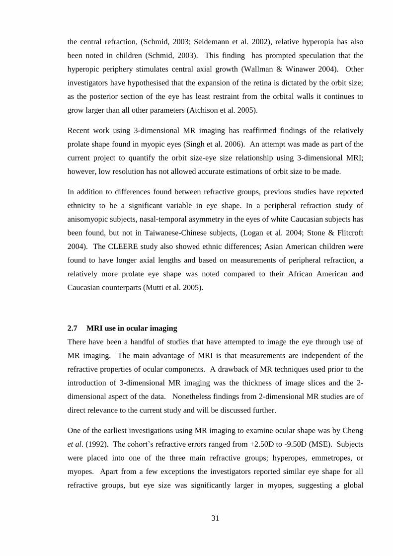
Figure 5 (a) The height and (b) the width measurements taken from MR images (from

Atchison et al. 2004) ............................................................................................................... 32

Figure 6 The effect of a steeper retina (R) on the tangential (T) and sagittal (S) image shells

(Dunne, 1995) ......................................................................................................................... 36

Figure 7 The effect of a flatter retina on the tangential and sagittal image shells (Dunne,

1995) ....................................................................................................................................... 37

Figure 8 Plot showing the average astigmatic axis direction and magnitude in the central 44°

for each of the three main refractive groups (from Seidemann et al. 2002) ........................... 39

Figure 9 (a) The uniform expansion of a myopic eye shown in Taiwanese - Chinese eyes (b)

the asymmetrical expansion of the nasal aspect shown in Caucasian subjects (from Logan et

al. 2004). ................................................................................................................................. 41

Figure 10 Diagram representing Traquair's depiction of the island of vision (right eye) ....... 44

Figure 11 Diagram showing the human visual pathway (LGN denotes the position of the

lateral geniculate nucleus). The diagram shows the crossover of the nasal fibres (temporal

field) to the contralateral side. The messages are relayed through the LGN and onto the

primary visual cortex located in the occipital lobe of the brain. ............................................. 48

Figure 12 Typical ERG waveform .......................................................................................... 52

Figure 13 Hexagon stimulus used in mfERG testing (from Marmor et al. ISCEV guidelines

2003) ....................................................................................................................................... 53

Figure 14 Typical waveform response from the mfERG (from Marmor et al. ISCEV

guidelines, 2003). .................................................................................................................... 54

Figure 15 3-dimensional topography plot of mfERG response (figure taken from subject data

set, left eye) ............................................................................................................................. 55

13

Figure 16 Cellular responses in mfERG (after Hood et al. 2002) .......................................... 56

Figure 17 Diagrammatical representation of the concentric ring averages analysed, note ring

1 denotes the presumed foveal response. ................................................................................ 58

Figure 18 Diagrammatical representation of the quadrant average analysis undertaken by

Kawabata and chi-Usami 1997. N.B the horizontal and vertical meridians have been omitted,

presumably to ensure equal hexagonal responses from each quadrant and also to exclude the

optic nerve head ...................................................................................................................... 59

Figure 19 On-centre ganglion cells and sinusoidal grating .................................................... 64

Figure 20 Visual resolution limit in cycles per degree at an eccentricity of 25˚, at radial

locations around the retina (Anderson et al. 1992) ................................................................. 67

Figure 21 (a) Equatorial stretching (b) Global expansion (c) Posterior Pole (after Strang et al.

1998) ....................................................................................................................................... 68

Figure 22 Graph showing the predicted decline in resolution with increasing myopia for each

of the three myopic models, (optical cut-off is marked at 45 cpd, represents the optical limit

of the eye) (after Strang et al. 1998) ....................................................................................... 69

Figure 23 An example of a Pentacam output. The output shows the corneal thickness for an

emmetropic subject (MSE: +0.50D). Further outputs are given for parameters such as

corneal curvature and aberrations. .......................................................................................... 75

Figure 24 The MR scanner and head coil (c/o Aston University Day Hospital) .................... 80

Figure 25 The three different views presented in mri3dX. Each view shows one slice ........ 81

Figure 26 The division of anterior and posterior volume measurements is shown by the

dashed line (after Gilmartin et al. 2008) ................................................................................. 82

Figure 27 Graphic depicting the 3-dimensional MRI process. The first image shows the raw

T2 weighted MR image. The second image shows the same scan once shaded using the mri

3dX program. The third image is a representation of the eye once the polygonal envelope

has collapsed around the shaded voxels producing a rough corrugated model of the eye

(Singh, Logan, & Gilmartin 2006). The final two pictures illustrate 3 dimensional models

post smoothing; radius bands (as described in Methods) are visible in the final picture. ...... 83

Figure 28 The direction in which data points are collapsed to generate data for the XQ. The

same methodology was applied to the +Q .............................................................................. 84

Figure 29 The diagram shows the conversion of 3D data to 2D. Figure provided c/o

Professor Bernard Gilmartin ................................................................................................... 85

Figure 30 Diagrammatical representation of the various parameters of ocular shape measured

as part of this study. ................................................................................................................ 89

14

Figure 31 Data plotted for the region 15-100% along the axis. 2nd

order polynomial fitted for

the region 25-75%. .................................................................................................................. 91

Figure 32 The equivalent radius of curvature by refractive group. Each data set is fitted with

a moving average trendline; averaging every second point .................................................... 93

Figure 33 Shows the standard deviation error bars for the emmetropic refractive group in the

region 15-92% along the axis ................................................................................................. 94

Figure 34 Shows the standard deviation error bars for the low myopic refractive group in the


Figure 35 Shows the standard deviation error bars for the highly myopic refractive group in

the region 15-92% along the axis ............................................................................................ 95

Figure 36 Shows the standard deviation error bars for the hyperopic refractive group in the


Figure 37 The equivalent radius data fitted with 6th

order polynomials to expose subtle

changes in shape ..................................................................................................................... 96

Figure 38 The anterior volumes (below in grey) and posterior volumes (above in black)

plotted as a function of MSE. Data is shown for RE only (n=73). ........................................ 97

Figure 39 The volume for the posterior 25% plotted as a function of MSE ........................... 98

Figure 40 The posterior volume minus the posterior 25% volume ........................................ 99

Figure 41 Corneal volume (via the Oculus Pentacam) vs. MSE (D) (p>0.05, r = -0.173) ... 100

Figure 42 A graphical representation of the retinal contours by quadrant ........................... 102

Figure 43 Nasal and temporal chord distances. Temporal chord distances were subtracted

from nasal and plotted graphically. The same methodology was used for S-I, SN-IT and ST-

IN quadrants. ......................................................................................................................... 103

Figure 44 Differences between the nasal and temporal chords in each refractive group ..... 104

Figure 45 Differences between the superior and inferior chords in each refractive group ... 105

Figure 46 Standard deviations for each refractive group, nasal-temporal quadrants ........... 106

Figure 47 Standard deviations for each refractive group, superior-inferior quadrants ......... 106

Figure 48 The differences between the SN and IT chords for each refractive group ........... 107

Figure 49 The differences between the ST and IN chords for each refractive group. NB

scaling differences of y axis compared to SN-IT chord differences graph ........................... 108

Figure 50 Standard deviations for each of the refractive groups SN-IT quadrants .............. 109

Figure 51 Standard deviations for each of the refractive groups ST-IN quadrants .............. 109

Figure 52 The maximum distance values at 5% or 2.5% increments along the presumed

visual axis.............................................................................................................................. 110

15


visual axis.............................................................................................................................. 111


visual axis.............................................................................................................................. 111


visual axis.............................................................................................................................. 112

Figure 56 Maximal distance from the presumed visual axis to the retinal surface for each

quadrant................................................................................................................................. 112

Figure 57 Maximum distance values at 5% or 2.5% increments along the presumed visual

axis ........................................................................................................................................ 115


axis ........................................................................................................................................ 115


axis ........................................................................................................................................ 116


axis ........................................................................................................................................ 116


quadrant................................................................................................................................. 117

Figure 62 The mean x² coefficient values for each quadrant divided further by refractive

group ..................................................................................................................................... 119

Figure 63 The mean x² coefficient values for the polynomial curves fitted to data

representing the posterior 25% cap of the eye. Data are separated by refractive group ...... 119

Figure 64 The mean x² coefficient values for each quadrant divided further by refractive

group ..................................................................................................................................... 120

Figure 65 The mean x² coefficient values for the polynomial curves fitted to data

representing the posterior 25% cap of the eye. Data are separated by refractive group ...... 121

Figure 66 The mean Interval Variance (IV) shown for the XQ ............................................ 122

Figure 67 The mean Interval Variance (IV) for the XQ meridians ...................................... 123

Figure 68 The mean Interval Variance (IV) for the +Q in the 25-75% region ..................... 124

Figure 69 The mean Interval Variance (IV) for +Q meridians ............................................. 125

Figure 70 The mean differences between the right and left eyes of emmetropic and myopic

refractive groups for the nasal and temporal quadrants. ....................................................... 126

Figure 71 The mean difference between the right and left eyes of emmetropic and myopic

refractive groups for the superior and inferior quadrants ..................................................... 127

Figure 72 Standard deviations (SD) for the nasal and temporal inter eye differences ......... 127

16

Figure 73 Standard deviations (SD) for the superior and inferior inter eye differences ....... 128


refractive groups for the SN and IT quadrants ...................................................................... 129


refractive groups for the ST and IN quadrants ...................................................................... 129

Figure 76 Standard deviations (SD) for the SN and IT inter eye differences ....................... 130

Figure 77 Standard deviations (SD) for the ST and IN inter eye differences ....................... 130

Figure 78 Central corneal thickness versus MSE (in D) as measured by the Oculus Pentacam

(n=42). All subjects from the MRI subject group were invited for Pentacam readings to be

taken, results are shown for subjects who responded (p= 0.051, r= -0.262). ....................... 131

Figure 79 Corneal thickness values (in microns) for the XQ, obtained using the Oculus

Pentacam (n=40) ................................................................................................................... 133

Figure 80 Graph of the mean uncorrected peripheral refractive error for right eyes fitted with

2nd

order polynomial curves (references to nasal and temporal refer to retinal not field

locations, n=42) .................................................................................................................... 148

Figure 81 Graphical representation of the mean difference in MSE between central and

peripheral locations, right eyes (linear fit used for emmetropic group, 2nd

order polynomials

for myopic groups) ................................................................................................................ 149

Figure 82 Mean J180 values for right eyes, fitted with 2nd

order polynomial curves............. 152

Figure 83 Mean J45 values for right eyes, fitted with linear trend lines ................................ 154

Figure 84 Graphical representation of cylindrical component, for right eyes only .............. 156

Figure 85 The difference in retinal contour data as derived by MRI and RetinaFit by field

angle (combined average of n=41) ....................................................................................... 157

Figure 86 Mean difference for y values between the MRI and RetinaFit techniques, with

reference to refractive error .................................................................................................. 159

Figure 87 The technique used to divide visual fields plots into quadrants. The greyed-out

regions show the position of the blind spot and the point directly above the blind spot, these

two points were excluded from analysis (as is standard in visual fields research). The circles

show the points which lie on the axes and the arrows show the quadrant into which these

circled points were included ................................................................................................. 166

Figure 88 The significant relationship between axial length (in mm) and mean spherical error

(MSE in D, n=40) (one tailed Pearson‘s correlation coefficient p<0.001, r = -0.854) ......... 168

Figure 89 Graph showing the mean sensitivity for each of the XQ quadrants, error bars show

standard deviations................................................................................................................ 169

17

Figure 90 Graph showing the mean MS response for each of the +Q quadrants, error bars

show standard deviations ...................................................................................................... 169

Figure 91 Mean TD per XQ quadrant, error bars show standard deviations ........................ 170

Figure 92 Mean TD per +Q quadrant, error bars show standard deviations......................... 171

Figure 93 Mean surface areas for each XQ quadrant are shown for the posterior 25% cap of

the eye. Error bars show standard deviations....................................................................... 172

Figure 94 Mean surface areas for each +Q quadrant are shown for the posterior 25% cap of

the eye. Error bars show standard deviations....................................................................... 173

Figure 95 IV indices per retinal quadrant, error bars show standard deviations .................. 174

Figure 96 IV per retinal quadrant, error bars show standard deviations ............................... 174

Figure 97 The fixation monitor visible to the investigator, the top left shows the signal

recorded................................................................................................................................. 180

Figure 98 The method by which mfERG rings and quadrants configurations were divided

before responses from each region were averaged and analysed ......................................... 181

Figure 99 Schematic representation of the angular subtense by the mfERG stimulus (NB not

to scale) ................................................................................................................................. 182

Figure 100 The PCI axial length against the mean spherical error (MSE) as measured by the

Shin Nippon autorefractor (n=23, left eye data) ................................................................... 183

Figure 101 N1 amplitudes shown as a function of retinal eccentricity (R5 indicates the ring

furthest from the fovea). Error bars show standard deviation of the dataset ....................... 183

Figure 102 P1 amplitudes shown as function of retinal eccentricity. Error bars show

standard deviation of the dataset ........................................................................................... 184

Figure 103 The N1 response amplitudes for +Q (LE data). Error bars show standard

deviation of the dataset ......................................................................................................... 185

Figure 104 The P1 response amplitudes for +Q (LE data). Error bars show standard

deviation of the dataset ......................................................................................................... 185

Figure 105 Surface areas and implicit times for the inferior-nasal retinal quadrant ............ 186

Figure 106 Shows the N1 response amplitudes for XQ (LE data) ....................................... 187

Figure 107 The P1 response amplitudes for the XQ (LE data). Error bars indicate the

standard deviation ................................................................................................................. 188

Figure 108 Shows P1 Implicit times for the XQ (LE data). Error bars indicate the standard

deviations .............................................................................................................................. 188

Figure 109 Surface areas and N1 implicit times for the inferior retinal quadrant ................ 189

Figure 110 Diagram showing the experimental setup (not to scale) .................................... 195

18

Figure 111 Subject OH, MSE: -8.62D. Vertical lines express 95% confidence limits, solid

lines show confidence limits for the detection function and dashed line for the direction

discrimination ....................................................................................................................... 199

Figure 112 Subject MN, MSE: -3.00D ................................................................................. 200

Figure 113 Subject AS, MSE: +0.50D ................................................................................. 201

Figure 114 Subject JA, MSE: +0.19D .................................................................................. 202

Figure 115 Diagrammatical representation of the surface area calculation of the ocular

surface. The grey band represents the 60-80% region for which area was calculated (not to

scale) ..................................................................................................................................... 205

Figure 116 Graphical representation of the spatial frequencies at which 50% of responses are

correct, plotted as a function of stretch index. Circles denote detection and stars indicate

direction discrimination. Case study RC is also included (see below). ............................... 206

Figure 117 Calculated index of stretch for subject OH: 93%. The graph shows the point

situated 40° from the presumed foveal location; the horizontal lines denote the distance from

the 40° location to the presumed visual axis (RE) Negative values denote the temporal

region and positive numbers denote the nasal. ..................................................................... 207

Figure 118 Calculated index of stretch for subject MN: 91% (RE). Negative values denote

the temporal region and positive numbers denote the nasal ................................................. 208

Figure 119 Calculated index of stretch for subject AS: 99% (RE). Negative values denote


Figure 120 Calculated index of stretch for subject JA: 92% (RE). Negative values denote the

temporal region and positive numbers denote the nasal ....................................................... 210

Figure 121 Case study: RC right eye .................................................................................... 211

Figure 122 Case study: RC left eye ...................................................................................... 212

Figure 123 Calculated index of stretch, subject RC, left eye: 104%. Negative values denote


Figure 124 Calculated index of stretch, subject RC, right eye: 81%. Negative values denote


Figure 125 Schematic illustration of the retinal layers of the human eye ............................ 220

Figure 126 Scanned copy of Aston University project consent by the Ethics Committee ... 242

Figure 127 Graph of the mean peripheral refractive error for left eyes fitted with 2nd

order

polynomial curves ................................................................................................................. 295

Figure 128 Graphical representation of the mean difference in MSE between the central and

peripheral locations, left eyes ............................................................................................... 296

Figure 129 Mean J180 values for left eyes, fitted with 2nd

order polynomial curves ............. 297

19

Figure 130 Mean J45 values for left eyes, fitted with linear trend lines ................................ 298

Figure 131 Peripheral refraction MSE results for subject RC .............................................. 315

Figure 132 MSE results for subject JP, with and without contact lenses in situ .................. 316

20

LIST OF APPENDICES

APPENDIX 1: LIST OF ABBREVIATIONS 240

APPENDIX 2: STUDY ETHICAL CONSENT FORMS AND INFORMATION 241

APPENDIX 3: OCULAR HEALTH AND HISTORY QUESTIONNAIRE 274

APPENDIX 4: MRI DERIVED AXIAL LENGTHS AND VOLUMES 277

APPENDIX 5: QUADRANT DATA FOR MRI WORK 282

APPENDIX 6: LEFT PERIPHERAL REFRACTION DATA 295

APPENDIX 7: RIGHT PERIPHERAL REFRACTION AND RETFIT DATA 300

APPENDIX 8: VISUAL FIELDS 317

APPENDIX 9: MFERG RING CONFIGURATION RESPONSES 330

APPENDIX 10: GANGLION CELL DENSITY: DETECTION TASK DATA 340

APPENDIX 11: GANGLION CELL DENSITY: DIRECTION DISCRIMINATION

TASK DATA 341

21

1 INTRODUCTION

Myopia is a refractive, and in some cases, pathological condition of the eye. Its prevalence

is widespread; in America an estimated 33.1% of the population have myopic refractive

errors (Vitale et al.2008) and in the Far East the figures are much greater with approximately

70% of Chinese adults affected (Edwards & Lam 2004). The worldwide prevalence of

myopia, the rapid increase in incidence over the past three decades (Bar et al. 2005; Vitale et

al. 2009), and its association with potential ocular morbidity and reduced quality of life, has

rightfully justified myopia as a key research topic in vision science, optometry, and

ophthalmology. In recent years myopia research has focused on identifying causes of

myopic development; subsequently specific types of ocular shape have been recognised as

possible precipitants of myopic development.

Higher levels of myopia are closely associated with a larger eye size. The expansion of the

eye can lead to adverse effects on the retinal tissue through tissue stretch and thinning. These

events may lead to reduced visual function, and less frequently, ocular morbidity.

Previously, imaging the eye has been limited to 2-dimensional approaches. The introduction

of 3-dimensional (3D) MR imaging permits a more accurate depiction of eye shape. The 3D

MRI provides a unique insight into previously inaccessible ocular areas, analysis of which

can be used to construct more comprehensive models of eye shape in myopia. Use of these

models can help further explain the processes by which ocular shape may cause or be

affected by myopic development.

The generation of myopic models, developed through ocular imaging, can also assist in

exploring theories of myopic ocular stretch and reduced visual function (Chen et al. 2006a;

Chui et al. 2005). Light sensitivity investigated through visual field testing has shown that

myopia as little as 2 dioptres (D) is capable of producing a significant reduction in sensitivity

compared with emmetropic (control) subjects (Martin-Boglind, 1991). Furthermore, reduced

responses in electrophysiological testing, more specifically mfERG have been noted in

myopic subjects (Chen et al. 2006a).

Although a strong association between reduced visual function and the presence of myopia

exists, the actual aspect of myopia causing the reduction remains equivocal. One possible

cause, and of particular interest to this study, is the theory that myopic ocular expansion

causes retinal stretch which leads to either retinal cell damage or reduced cell density and

22

subsequently a reduction in visual sensitivity. It has been predicted that approximately 15D

of refractive error leads to twice the spacing between retinal neurons compared to that found

in an emmetrope (Chui et al. 2005).

In this study the functional responses from different retinal layers are evaluated through

measurements obtained from various investigative techniques. Findings are then compared

with specific indices of ocular shape obtained through 3-dimensional MR imaging. One of

the principal aims of the present study is to correlate localised areas of retinal shape with

tests of visual functionality in myopic and emmetropic subjects. It is envisaged that this type

of investigation will help determine whether retinal shape affects the visual function of the

eye.

This thesis is comprised of two main sections; the first part describes investigations of

ocular shape through use of 3-dimensional MRI, peripheral refraction, and further biometric

measurements taken through use of commercially available instruments such as the Zeiss

IOL Master and Oculus Pentacam. The second part of the thesis focuses on aspects of visual

function determined by visual field tests, multifocal electroretinograms, and ganglion cell

density. The tests of visual function are then correlated with specific indices of ocular shape

as derived through MR imaging.

The thesis concludes by outlining the principal findings and discusses their relevance to

clinical practice. Scope for further research is provided with explanations of how the current

data set could be expanded to investigate further parameters of ocular structure and function.

23

2 OCULAR SHAPE IN MYOPIA

Myopia is well established as a refractive and structural defect of the eye. An excessively

long vitreous chamber depth relative to the corneal and lenticular refracting properties

renders the eye myopic. Expansion of the eye in myopia is not, however, limited to the axial

meridian; both the width and height of the eye have been reported to increase in size

(Atchison et al. 2005). Accurate representation of eye shape is the centrepiece to

understanding myopia, as shape can provide clues to the course of ocular expansion taken by

the myopic eye, the possible effects on visual function, and facilitate the development of

therapies against myopia.

2.1 Factors influencing eye growth

The eye is a unique organ; both its physical and sensory development is dependent on visual

experience, albeit to differing amounts. In a similar way to many bodily organs, the eye has

reportedly shown a subtle form of homeostatic control with regards to ametropic

development, (Wallman & Winawer, 2004). The control, however, is defective because in

many cases ametropia still develops.

Animal studies in general have shown that in the developing eyes of neonate animals,

myopic defocus produced by the introduction of positive power spectacle lenses can inhibit

the natural elongation of the eye, or promote excessive elongation with negative lenses (i.e.

hyperopic defocus). Positive lenses have been found to elicit a much more powerful

response than negative lenses. The choroid is known to thicken transiently with the

introduction of positive lenses and choroidal thinning occurs with negative lenses (Wallman

&Winawer, 2004; Zhu et al. 2005). The exact mechanisms by which the eye recognises the

defocus is unknown, although it appears that a trial and error method is unlikely (Zhu et al.

2005). A parallel can be drawn with form deprivation studies in animals, where depriving

the eye of visual experience, fully or partially, can cause the globe to expand. Similar

findings have also been reported in human subjects in whom congenital defects such as

ptosis or corneal defects have created a barrier to visual input (Twomey et al. 1990; O‘Leary

& Millodot, 1970). There is no definitive answer to the question of why form deprivation

causes such excessive growth. One idea used to explain growth during form deprivation is

that the fovea recognises there is no visible image anterior to it and so the only other possible

location is posterior; and thus in an attempt to achieve a focused image the eye elongates. In

24

effect the eye is ‗searching‘ for the image‘ (Wallman & Winawer, 2004). Alongside the

reported increase in ametropia with form deprivation, runs the theory that a peripheral

refractive error which is more hyperopic than the central refraction, may precipitate axial

growth (see 3.1).

The fact that visual experience could influence development of ametropia is significant to

development of therapies in myopia prevention. The refractive status of the peripheral and

central visual fields could be manipulated by the use of optical corrections such as custom

made contact lenses; minimising the relative peripheral hyperopia. The prospect of

pharmacological therapies to prevent myopia has also been studied in depth (Bartlett et al.

2003; Gilmartin, 2004; McBrien et al. 2008; Siatkowski et al. 2004).

2.2 Ocular biometric studies

In addition to the differences in global eye shape and size, characteristics of internal ocular

refractive components have been associated with myopia. One of the most influential ocular

biometric studies was that of Stenström (1948), he concluded that axial length was the

principal cause of all refractive error. Many others went on to reanalyse Stenström‘s classic

data set and of particular significance is Van Alphen‘s analysis (1961). Van Alphen

concluded that the myopic eye had a longer axial length and could also be associated with

increased corneal curvature and a flatter crystalline lens. Sorsby, (Benjamin et al. 1957;

Sorsby & Leary 1969) disputed these reports, arguing that only myopic error greater than

4D could be solely attributable to excessive axial elongation. Sorsby believed that myopia

less than 4D could be due to any individual refracting component.

Axial length measurements can be made through numerous methods; currently one of the

most popular techniques is the non invasive partial coherence interferometry (PCI) method

employed by the Zeiss IOL Master (see 7.3).

2.3 Axial length in myopia

There is a plethora of research suggesting increased longitudinal axial length is the main

structural correlate of myopia (see Figure 1). The ocular region which contributes most to

the increase in axial length is the vitreous chamber (Garner et al. 2006; Goss et al. 1997;

McBrien & Millodot 1987). Excessively long axial length appears to be the main structural

correlate for both early and late onset myopia (Jiang & Woessner, 1996; McBrien & Adams

25

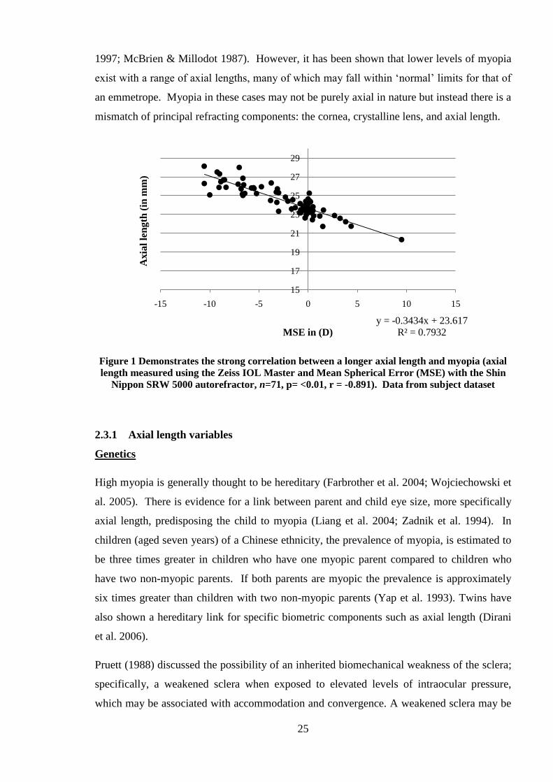
1997; McBrien & Millodot 1987). However, it has been shown that lower levels of myopia

exist with a range of axial lengths, many of which may fall within ‗normal‘ limits for that of

an emmetrope. Myopia in these cases may not be purely axial in nature but instead there is a

mismatch of principal refracting components: the cornea, crystalline lens, and axial length.

Figure 1 Demonstrates the strong correlation between a longer axial length and myopia (axial

length measured using the Zeiss IOL Master and Mean Spherical Error (MSE) with the Shin

Nippon SRW 5000 autorefractor, n=71, p= <0.01, r = -0.891). Data from subject dataset

2.3.1 Axial length variables

Genetics

High myopia is generally thought to be hereditary (Farbrother et al. 2004; Wojciechowski et

al. 2005). There is evidence for a link between parent and child eye size, more specifically

axial length, predisposing the child to myopia (Liang et al. 2004; Zadnik et al. 1994). In

children (aged seven years) of a Chinese ethnicity, the prevalence of myopia, is estimated to

be three times greater in children who have one myopic parent compared to children who

have two non-myopic parents. If both parents are myopic the prevalence is approximately

six times greater than children with two non-myopic parents (Yap et al. 1993). Twins have

also shown a hereditary link for specific biometric components such as axial length (Dirani

et al. 2006).

Pruett (1988) discussed the possibility of an inherited biomechanical weakness of the sclera;

specifically, a weakened sclera when exposed to elevated levels of intraocular pressure,

which may be associated with accommodation and convergence. A weakened sclera may be

y = -0.3434x + 23.617

R² = 0.7932

15

17

19

21

23

25

27

29

-15 -10 -5 0 5 10 15

Axia

l le

ng

th (

in m

m)

MSE in (D)

26

vulnerable to ocular expansion, (Pruett, 1988). With the identification of genes that cause

myopia, the mechanisms causing growth may be identified and effective treatment options

developed, (Young et al. 2007).

Gender

Gender differences in axial length have been observed in both children and adults. A large

scale study on Australian school children found boys to have longer axial length than girls

by approximately 2.45% (Ojaimi et al. 2005); similar results have been noted in young adults

where average female axial length was approximately 1.97% shorter than males (Logan et al.

2005).

Accommodation

Axial length is thought to increase when accommodation is active, conflicting evidence

exists as to whether this increase in axial length is more prominent in myopic or emmetropic

subjects (Mallen et al. 2006; O' Donoghue et al. 2005). For near objects convergence is

closely associated with accommodation. The isolation of convergence, with little active

accommodation, has also shown increases in axial length (Bayramlar et al. 1999).

Diurnal variations

There have been reports of diurnal variations in the axial lengths of both humans and

animals (Liu & Farid 1998; Stone & Flitcroft 2004). These fluctuations are thought to be

small, between 15-40µm, and present on an irregular basis. In some subjects the diurnal

fluctuations may not occur at all. Diurnal variations in axial length may occur due to

disruptions in normal light levels or as part of a hormone/neurotransmitter related response.

Intraocular pressure (IOP)

In general it has been agreed that a higher IOP may be associated with longer axial lengths,

(Tomlinson & Phillips 1970; Tomlinson & Phillips 1972; Tsutsui et al. 2003). This claim is

not supported in children, suggesting the IOP-axial length association may only be present in

subjects with fully developed eyes (Lee et al. 1999).

Stature

Saw et al. examined the link between height and its relationship with refractive error and

ocular biometry in Singaporean Chinese children (aged 7-9 years old), (Saw et al. 2002).

They found girls who were taller had longer axial lengths, deeper vitreous chambers, flatter

27

corneas and their refractions tended to be more myopic. It was also found that boys who

were heavier in weight tended to be slightly more hyperopic and have shorter vitreous

chambers.

Orbit size

Atchison et al. suggested that the growth of the eye was limited by orbit size. They

suggested the excessive growth in the axial meridian was a consequence of less restriction by

the orbit in the posterior section of the eye, (Atchison et al. 2004). The claims are contrary

to the findings of a study examining Chinese myopic eyes using MR imaging, where no

association was found between ocular and orbit size (Chau et al. 2004). Notably ethnic

variations in eye shape have previously been reported (Logan et al. 2004). Thus far no large

scale study has examined the relationship between ocular and orbit size in any other ethnic

group.

2.4 Cornea and myopia

The cornea is an avascular and transparent structure covering part of the anterior eye. The

typical corneal diameter is approximately 12.89±0.60 mm (Martin & Holden 1982) and

typical central thickness readings by ultrasound pachymetry have been reported as 542±33

μm (Marsich & Bullimore 2000). The typical corneal power in an adult eye is 43D, and

accounts for approximately two thirds of the eye‘s total refractive power. Corneal power is

related to its curvature. A steeper radius of curvature corresponds to a more myopic corneal

power; this is most commonly expressed in millimetres (mm) or dioptres (D). Average

corneal curvature is 7.80mm in an adult eye. The cornea is the source of most astigmatic

error, although some astigmatism may infrequently originate from the crystalline lens.

Corneal curvature

The cornea in myopia is often studied in reference to the axial length. Grosvenor suggested

the presence of a relationship known as the Axial Length: Corneal Radius ratio (AL:CR

ratio) (Grosvenor 1988). This method of analysis has subsequently been used in several

studies that followed (Goss et al. 1997; Grosvenor & Goss 1998). Grosvenor suggested that

a high level AL:CR (i.e. greater than 3) was a risk factor for myopic development in

emmetropic youths (see Figure 2). In children a higher AL:CR is also believed to be a risk

factor for developing myopia, however, for adult onset myopia AL:CR has not proved to be

significantly different to emmetropes, (McBrien & Adams 1997).

28

Figure 2 Graphical representation of the AL:CR ratio as calculated from readings taken with

the Zeiss IOL Master (n=66). Data presented from subject dataset

Grosvenor and Goss reported that longer eyes tended to have flatter corneas, this finding has

been reconfirmed by more recent work, (Chang et al. 2001). However, myopic eyes have

been found to have steeper corneas than those of emmetropes (Garner et al. 2006; Goss et al

1997). In particular it has been reported that in myopes the vertical meridian is steeper than

the horizontal, (Goss & Erickson 1990). This finding may help elucidate the direction in

which myopic stretch takes place.

Further differences in corneal curvature are noted when examining measurements with

reference to ethnicity. Ethnicity differences in corneal curvature have been reported in both

adults (Logan et al. 2005) and in children (Twelker et al. 2009). Additionally, gender

differences in the corneal curvature of children have also been noted; females have been

reported as having significantly steeper corneas compared to males (Gwiazda et al. 2002).

y = -0.058x + 3.0223

R² = 0.6787

2

2.2

2.4

2.6

2.8

3

3.2

3.4

3.6

3.8

4

-15 -10 -5 0 5 10

AL

:CR

ra

tio

MSE (in D)

29

Figure 3 Graphical representation of the average keratometry reading as measured with the

Zeiss IOL Master against MSE (n=66). Data presented from subject dataset

Evaluation of the corneal topography has also produced interesting findings; increasing

myopia shows a tendency for the cornea to flatten less rapidly as it approaches the corneal

periphery. This is particularly the case for myopic error greater than approximately -4.00D,

(Carney et al. 1997; Zadnik et al. 1999). A reduction in the flattening of the corneal

periphery has been noted with increasing vitreous depth (Carney et al. 1997).

Corneal thickness

The average corneal thickness in humans is approximately 542±33μm. There are many

variables for corneal thickness; race, gender, and diurnal variations are all evident (Hamilton

et al. 2007). Further physical changes of the cornea, on a cellular level, have shown

endothelial cell density to be reduced in myopic subjects. Chang et al. indicate that the

corneal endothelium is able to operate with very low cell density, therefore a significant

effect on visual function is unlikely (Chang et al. 2001).

2.5 Anterior chamber depth and myopia

The average anterior chamber depth is 3.33±0.61mm as measured with the Zeiss IOL Master

(Reddy et al. 2004), this value gradually decreases with age. Both the Zeiss IOL Master and

the Oculus Pentacam allow for rapid non-contact measurements of the anterior chamber (see

7.2 and 7.5).

y = 0.029x + 7.824

R² = 0.1491

6

6.5

7

7.5

8

8.5

9

-13 -8 -3 2 7

Av

era

ge

K r

ead

ing

(in

mm

)

MSE (in D)

30

In general the anterior chamber depth in myopes has been found to be deeper than

emmetropes (Bullimore et al. 1992; Garner et al. 2006; Logan et al. 2005). It has been

proposed that the thinning of the crystalline lens may contribute to the increased depth of the

anterior chamber (Garner et al. 2006), or it may be a consequence of the ocular stretch which

is synonymous with increasing myopia. Figure 4 shows the anterior chamber depth

measured using the Zeiss IOL Master in subjects who formed part of the cohort of the

current study.

Figure 4 Graphical representation of anterior chamber depth (as measured with the Zeiss IOL

Master) with MSE n=69 (p= <0.01. r= 0.427). Data presented from subject dataset

2.6 Eye shape and retinal contour in myopia

There is widespread agreement that the average size of the eye in myopia is generally larger

than that of an emmetrope or hyperope (Atchison et al. 2004; Atchison et al. 2005;

Gilmartin, 2004; Logan et al. 2005; Singh et al. 2006). There is also general agreement that

the increase in axial length is the most pronounced of all the changes in the size of the

myopic eye. Differences of opinions exist when considering other parameters such as retinal

contour, height and width of the eye in myopia. These uncertainties exist largely due to

limitations in ocular imaging techniques (Stone & Flitcroft 2004). Many previously

employed techniques measured along the axial dimension only, and measures such as retinal

contour were inferred rather than directly measured.

Through peripheral refraction studies the myopic eye has typically been found to be prolate

or less oblate in shape than emmetropic and hyperopic eyes (Logan et al. 2004). Previous

work has also shown that myopes tend to have hyperopic peripheral refractions relative to

y = -0.0318x + 3.4967

R² = 0.1857

1.5

2

2.5

3

3.5

4

4.5

5

-13 -8 -3 2 7

AC

dep

th (

in m

m)

MSE (in D)

31

the central refraction, (Schmid, 2003; Seidemann et al. 2002), relative hyperopia has also

been noted in children (Schmid, 2003). This finding has prompted speculation that the

hyperopic periphery stimulates central axial growth (Wallman & Winawer 2004). Other

investigators have hypothesised that the expansion of the retina is dictated by the orbit size;

as the posterior section of the eye has least restraint from the orbital walls it continues to

grow larger than all other parameters (Atchison et al. 2005).

Recent work using 3-dimensional MR imaging has reaffirmed findings of the relatively

prolate shape found in myopic eyes (Singh et al. 2006). An attempt was made as part of the

current project to quantify the orbit size-eye size relationship using 3-dimensional MRI;

however, low resolution has not allowed accurate estimations of orbit size to be made.

In addition to differences found between refractive groups, previous studies have reported

ethnicity to be a significant variable in eye shape. In a peripheral refraction study of

anisomyopic subjects, nasal-temporal asymmetry in the eyes of white Caucasian subjects has

been found, but not in Taiwanese-Chinese subjects, (Logan et al. 2004; Stone & Flitcroft

2004). The CLEERE study also showed ethnic differences; Asian American children were

found to have longer axial lengths and based on measurements of peripheral refraction, a

relatively more prolate eye shape was noted compared to their African American and

Caucasian counterparts (Mutti et al. 2005).

2.7 MRI use in ocular imaging

There have been a handful of studies that have attempted to image the eye through use of

MR imaging. The main advantage of MRI is that measurements are independent of the

refractive properties of ocular components. A drawback of MR techniques used prior to the

introduction of 3-dimensional MR imaging was the thickness of image slices and the 2-

dimensional aspect of the data. Nonetheless findings from 2-dimensional MR studies are of

direct relevance to the current study and will be discussed further.

One of the earliest investigations using MR imaging to examine ocular shape was by Cheng

et al. (1992). The cohort‘s refractive errors ranged from +2.50D to -9.50D (MSE). Subjects

were placed into one of the three main refractive groups; hyperopes, emmetropes, or

myopes. Apart from a few exceptions the investigators reported similar eye shape for all

refractive groups, but eye size was significantly larger in myopes, suggesting a global

32

expansion model of the myopic eye. The study also measured sclera and choroidal thickness

which were uniformly thinner across the globes of the myopic eyes.

Miller et al. carried out MRI scans of seventy-eight subjects using a 1.5 tesla MR scanner. A

difference in axial length between the hyperopic and myopic eyes was reported. To a lesser

extent, equatorial distances of myopic eyes were noted as larger compared to hyperopic eyes

(Miller et al. 2004). In a similar study Atchison et al. (2004) scanned eighty-eight young

adult subjects using a 1.5 tesla MR scanner. Specifically differences between emmetropic

and myopic eye sizes was investigated; refractive errors ranged from +0.75 to -12D MSE.

Notably the number of emmetropes was fewer than myopes; 22 and 66 respectively. The

scans were analysed by measuring the width and height in millimetres. Measurements of

length were taken from the posterior pole (P) to the anterior cornea (A), measurements of

width were taken from the widest regions from nasal (N) to temporal (T) retina, and

measurements of height were taken from the superior (S) to inferior (I) retina (see Figure 5).

Figure 5 (a) The height and (b) the width measurements taken from MR images (from Atchison

et al. 2004)

Myopic eyes were found to be larger in all three meridians. The heights and widths of

emmetropic eyes were not significantly different. In myopes the heights were noted to be

longer than the widths. Atchison et al. went on to mathematically analyse data on retinal

shape for the same subject group through fitting of ellipsoids using specialised software;

from this work it was reported that the shape of a myopic eye was less oblate than that of an

emmetropic eye.

The aforementioned studies have provided valuable data; however, they have all been

limited by producing only a 2-dimensional view of the eye (see Figure 5). Furthermore, the

a b

Illustration removed for copyright restrictions

33

data are limited in the number of MR slices taken. If we assume an axial length of 21mm, a

3mm size slice would equate to seven slices in the axial meridian, thus missing

approximately two thirds of the data. Further work by Singh et al. (2006) has developed 3-

dimensional MR scanning with smaller MR slices and thus a more accurate depiction of

ocular shape, (see section 7.6). In brief, the method involves the use of a 3 tesla Siemens

whole body MR scanner. Previous MR ocular imaging studies have in general used T1

weighted images; the 3D MR technique uses T2 weighted images. The contrast of the T2

images is optimised to distinguish the fluid filled ocular structures from the bony orbit. The

3-dimensional aspect is achieved through use of a modified version of freeware software

MRi3dx. The program allows the eye to be shaded with 1mm³ voxels, which are assigned

x,y coordinates so data can be plotted graphically. Various parameters are generated by the

program for example ocular volume (Gilmartin et al. 2008), surface area and radius of

curvature (see 9.5).

Since the introduction of 3-dimensional ocular MRI there has been a recent attempt at

imaging the eye using a 7 tesla scanner, which enables the production of higher resolution

images. The use of higher field strengths does, however, make the image more prone to

motion artefacts; in the case of ocular imaging small eye movements may be problematic.

Additionally it is more difficult to ascertain specific absorption rate (SAR) safety levels;

scanning at higher field strength can create discomfort for subjects. The 3 tesla field strength

used for ocular imaging is sufficient for examining ocular volume (Richdale et al. 2009), but

for smaller structures such as the cillary body or crystalline lens a higher field strength

would be more appropriate.

2.8 Summary

Imaging the eye in vivo has proven problematic; the most widely available technique to

derive eye shape appears to be through transformation of peripheral refraction data.

Peripheral refraction is often achieved by laboratories customising existing autorefractors.

Although peripheral refraction is flexible and relatively inexpensive there is a lack of

standardisation and the extent of the field measured is limited by factors such as pupil size.

Further evaluations of eye shape have been made through 2-dimensional (2D) MR imaging,

however this technique has also demonstrated limitations in accessibility and data analysis.

3-dimensional (3D) MRI, which is used in the current study, overcomes limitations imposed

by both 2D MR imaging and peripheral refraction. 3D MRI has shown the ability to

34

calculate ocular surface curvature and volume, it is envisaged that further biometric

parameters will also be analysed using this technique. It is acknowledged that whilst 3D

ocular MRI is an invaluable tool for assessing more global parameters such as ocular volume

and eye size, higher resolutions are required to detect smaller internal ocular structures. This

thesis will attempt to evaluate more global measures of ocular shape in the context of

different refractive groups.

35

3 PERIPHERAL REFRACTIVE ERROR AND OCULAR SHAPE

3.1 Introduction

Off axis refractive error has been used for several decades to evaluate peripheral aberrations

and infer retinal contour. Of particular interest to the field of myopia is the investigation of

the theory that relative to the central refractive error a hyperopic peripheral refraction may

precipitate axial growth of the eye, which in turn leads to myopic ametropia (Smith et al.

2007; Wallman & Winawer 2004).

3.2 Peripheral refraction techniques

Peripheral refractive error may be measured through objective or subjective techniques.

Earlier studies tended to use a combination of retinoscopy and subjective refraction, similar

to standard on-axis refraction. Retinoscopy is an objective, flexible and widely available

technique; however, as the angle of eccentricity from the fovea increases there is a

concurrent increase in oblique off axis astigmatism making retinoscopy more challenging

and prone to errors. Furthermore, retinoscopy is not practical for examining large cohorts

due to the time and proficiency required to obtain accurate measurements. Owing to poor

peripheral acuity the standard subjective refraction which often follows retinoscopy, in a

normal clinical eye test, can be difficult for subjects when attempted away from the visual

axis.

Earlier peripheral refraction studies used manual optometers, but their lack of reproducibility

and high levels of peripheral aberrations has led to a decline in their usage (Fedtke et al.

2009). More recent peripheral refraction work has made use of commercially available

autorefractors which require modifications by investigators in order to present targets off

axis. Autorefractors allow an objective measure of refractive error and measurements are

free from both practitioner and subject bias. There are, however, a number of limitations:

autorefractors are rarely able to measure further than 30-40° eccentricity, additionally they

have been shown to overestimate myopia due to the accommodative effort exerted by the

subject as he or she becomes aware of the fixation target‘s proximity to the eye. Use of

cycloplegic drugs can temporarily paralyse the accommodative effort and overcome

instrument myopia; additionally the mydriatic effect facilitates the measurement of

peripheral readings. There are several binocular open view autorefractors available, which

can also help reduce levels of instrument myopia.

36

3.3 Peripheral astigmatism

Obliquely incident light rays from objects positioned in the peripheral visual field are limited

by the pupil size, consequently they are refracted asymmetrically into two mutually

perpendicular planes; tangential and sagittal, giving rise to oblique astigmatism. The

tangential meridian contains the optic axis and corresponding meridional ray.

The difference between the tangential and sagittal focal lines; the interval of Sturm,

represents the magnitude of astigmatic error. Light leaving the eye and into the object plane

is also susceptible to oblique astigmatism; this is equal and opposite to the value of oblique

astigmatism for light entering the eye. For a given eccentricity the oblique astigmatism

value for light leaving the eye is equal to the refractive error of the eye. The difference

between oblique astigmatism from the object plane and the oblique astigmatism from the

image plane can be used to calculate peripheral astigmatism. As the angle of eccentricity

increases the sagittal image shell falls further away from the retina, becoming increasingly

hyperopic. The tangential image shell becomes more myopic with increasing eccentricity

(Dunne 1995). The peripheral astigmatism values therefore increase with increasing

eccentricity.

Figure 6 The effect of a steeper retina (R) on the tangential (T) and sagittal (S) image shells

(Dunne, 1995)

37

Figure 7 The effect of a flatter retina on the tangential and sagittal image shells (Dunne, 1995)

3.3.1 Peripheral astigmatism and refractive error

Thomas Young (1801) is often attributed as being the first to note the presence of oblique

aberrations in the form of peripheral astigmatism. Young‘s early attempts at modelling the

sagittal and tangential image shell curvatures have been confirmed since by investigations on

both human and schematic eyes.

In 1931, Ferree, Rand, and Hardy sought to classify peripheral astigmatism. A Zeiss parallax

optometer was used to examine peripheral refraction of 21 eyes at 5° intervals in the

horizontal meridian up to a maximum of 60°. 18 of the eyes fell into one of two categories,

labelled Type A and Type B. The remaining 3 eyes showed disparity between the nasal and

temporal meridians and were classified as a separate entity.

Subjects classed as Type A were shown to be relatively myopic as the angle of eccentricity

increased, and the vertical meridian more hyperopic. Type B subjects were shown to be less

myopic with increasing eccentricity and more hyperopic in the vertical meridian (Ferree et

al. 1931).

Millodot (1981) sought to further examine the inter refractive group variability. Using a

cohort of 62 eyes, Millodot measured peripheral refraction with a Topcon refractometer at

10° intervals along the horizontal meridian up to a maximum of 60°. Millodot found the

peripheral astigmatic error to increase with increasing eccentricity in 91% of the eyes tested.

Three main refractive groups were examined; myopes, hyperopes and near emmetropes. He

38

noted significant differences in the type of astigmatism between each refractive group, but

the magnitude of astigmatism was not significantly different.

Lotmar and Lotmar (1974) analysed results from an earlier study by Rempt et al. which had

examined 363 subjects using retinoscopy. Through calculation of values for the interval of

Sturm, using Gullstrand‘s schematic model eye, Lotmar and Lotmar sought to classify the

eyes into the two sub types (A and B) as proposed by Ferree et al. They concluded that a

clear distinction into Type A or Type B eyes could not be made.

An insightful method of evaluating peripheral astigmatism by Seidemann et al. plotted the

average peripheral astigmatic axis in the central 44° for the three main refractive groups (see

Figure 8). The two eyes displayed a ‗mirror effect‘ in their axis orientation and degree of

astigmatic error (shown in Figure 8). Interestingly, levels of astigmatism were noted to be

smaller in the nasal retina compared to the temporal retina and also the fovea. Larger

astigmatic error in the temporal retina was also noted by a previous study by Dunne and

Barnes (1987). Seidemann et al. noted that their results showed unusually high cylindrical

errors and thus the mean spherical errors were more myopic in comparison to previous

studies.

39

Figure 8 Plot showing the average astigmatic axis direction and magnitude in the central 44°

for each of the three main refractive groups (from Seidemann et al. 2002)

3.4 Computational approach to deriving retinal contour

Dunne (1995) utilised the properties of peripheral astigmatism to devise a computer program

aimed at profiling retinal contour. The program is based upon the positions of the tangential

and sagittal image shells. The fact that a change in retinal contour brings about a change in

the two image shells is exploited by the program.

An approximate schematic model is used in which the sagittal image shell travels towards

becoming more myopic, and tangential towards a more hyperopic dioptric distance. The two

image shells then move towards each other at an equal rate; this process enables the mean

spherical error to be calculated, diminishing the effect of peripheral astigmatism.

40

Corneal asphericity is adjusted so that the peripheral astigmatism matches the measured data.

Retinal curvature is then adjusted, and the sagittal and tangential refractive errors calculated.

The retinal contour coordinates can be used to estimate values of apical radii and conic

constants. These are inputted into further equations to eventually derive values of x and y

which can be plotted graphically (see 11.7).

3.5 Retinal profile and peripheral refraction

Ferree, Rand and Hardy‘s work into peripheral astigmatism served as a basis for the theory

that the differences noted on the skiagrams they plotted may originate from changes in the

retinal shape (Ferree & Rand, 1933). Certainly for years axial length had been known to be

a major structural correlate of central refractive error, however as previously mentioned,

peripheral refractive measures may not be directly indicative of axial length. To date, few

studies have investigated axial length at peripheral retinal points and correlated it with mean

spherical error. Schmid (2003) examined axial length and refractive error in a large cohort

of children, at an eccentricity of 30° only. Mallen and Kashyap (2007) investigated the

effect in a small group of adults, for the central 80°. A significant correlation between mean

spherical error and axial length was noted in both studies. However factors such as lens tilt

and curvature may confound off-axis readings and there may be adverse effects from corneal

curvature and pupil diameter (Atchison 2004).

In the early 1970s, Rempt, Hoogerheide, and Hoogenboom carried out a series of peripheral

refraction studies which triggered tremendous amounts of interest regarding the relationship

between progression of myopia and peripheral refraction. A widely cited study (Hoogerheide

et al. 1971) investigated the reasons why trainee pilots who were initially emmetropic went

on to develop myopia whereas others, who were exposed to the same environmental

conditions, did not. Amongst other refractive and functional measures, the investigators

used retinoscopy to measure peripheral refractive error. The pilots who went on to develop

myopia were generally found to be relatively hyperopic in the periphery. It has since been

widely hypothesised that a relatively hyperopic periphery may encourage axial growth and

thus myopia (e.g. Chen et al. 2010, Smith et al. 2007; Wallman and Winawer 2004).

The theory that the peripheral retinal shape or refractive error may influence central growth

has received further support from studies on infant rhesus monkeys (Macaca mulatta).

Elimination of central foveal contributions through foveal ablation have shown ocular

41

growth and emmetropisation processes to be unaffected; leading to the assumption that

peripheral vision may independently mediate central growth (Smith et al. 2007).

Studies have examined peripheral refraction with reference to various parameters such as

central refraction, ethnicity, age and gender (Logan et al. 2004; Mutti et al. 2000)

Logan et al. advanced previous findings by measuring peripheral refraction and using it to

determine retinal contour in a group of 56 young adult subjects (Logan et al. 2004). Subjects

were sub divided by ethnicity; Caucasian or Taiwanese-Chinese and then by type of myopia;

anisometropia or isomyopia (see Figure 9). Cycloplegic peripheral refractions were taken

using a Canon R-1 infra red open field autorefractor, in the horizontal meridian at 5°

intervals to a maximum eccentricity of 35±5°. Axial length and corneal curvature measures

were also taken using commercially available equipment at the time, along with A scan

ultrasonography and fundus photography. Logan et al, transformed peripheral refractive

data to represent retinal contours by use of a computational approach (Logan et al 1995;

Dunne et al. 1995).

Figure 9 (a) The uniform expansion of a myopic eye shown in Taiwanese - Chinese eyes (b) the

asymmetrical expansion of the nasal aspect shown in Caucasian subjects (from Logan et al.

2004).

42

Although globe enlargement was noted in both ethnic groups with increasing myopia,

asymmetries between the nasal and temporal quadrants were noted in the Caucasian subjects

only. Greater expansion was inferred from the nasal retinal periphery. In contrast,

Taiwanese-Chinese subjects displayed greater homogeneity between nasal-temporal retinal

contours. Nasal-temporal differences have subsequently been noted in many later studies

(e.g. Atchison et al. 2006; Mallen and Kashyap, 2007; Pardhan and Rae, 2009). The

temporal peripheral refractive errors have been shown to correlate with central refractive

error better than nasal (r = -0.633, p= <0.001) (Pardhan and Rae, 2009).

The general consensus is that myopic eyes tend to be relatively hyperopic in the periphery

and hyperopic and emmetropic eyes relatively myopic (Chen et al. 2010). One exception is a

study by Seidemann et al., who found all three main refractive groups to be relatively

myopic in the periphery. They did, however, acknowledge that their measurements showed

unusually large astigmatic errors, which would contribute to a more myopic spherical

equivalent. The relative increase in myopia in the periphery of myopes was reported to be

less when compared to emmetropic and hyperopic subjects.

The effect of a relatively hyperopic periphery in myopes and the opposite in hyperopes and

emmetropes has been reported to be present in younger age groups. Large cohort studies in

children (n=822 ) aged 5-14 years, have shown through cycloplegic retinoscopy that myopic

children show hyperopic shifts at 30° eccentricity relative to the centre, by an average of

+0.80 ± 1.29 D, (Zadnik et al. 1999).

3.5.1 Vertical peripheral refraction

Very few studies have collected data on vertical peripheral refraction; this is largely due to

instrumental limitations in obtaining measurements in this meridian.

Seidemann et al. (2002) used a double pass technique and Powerrefractor to measure

horizontal peripheral refraction of the three main refractive groups; emmetropic, myopic and

hyperopic. The spherical equivalent refraction was found to be more myopic in the superior

retina than the inferior by an average of 0.17D for every 10 degrees increase in eccentricity.

The results are in line with more recent findings reported by Mallen and Kashyap (2007),

who describe a technique to estimate retinal contour using a modified Zeiss IOL Master.

43

The results showed the superior field (inferior retina) in myopic eyes to be relatively

hyperopic compared with inferior field.

Atchison et al. (2006) compared peripheral refractive error in young adult (18-35 year old)

myopic (up to -12D) and emmetropic subjects. Measurements were taken using the Shin

Nippon SRW 5000 autorefractor at 5° intervals up to 35° in the horizontal (n=116 eyes) and

vertical meridians (n=43 eyes). In the horizontal meridians the temporal spherical

equivalent error was significantly affected by central refractive error at eccentricities of 20-

25° and beyond, in the nasal aspect these changes occurred much sooner at 5° and beyond.

In the vertical meridian all refractive groups were found to have a relatively myopic shift,

but not as a function of central myopic error.

3.6 Summary

The retinal area measured by peripheral refractive error is limited by pupil size; few

investigators manage to take readings beyond 30-40˚ eccentricity. Additionally, areas of the

retina are missed due to measurements being taken at 5-10˚ intervals only. Further

limitations can arise from refractive component misalignment, and curvature changes with

increasing eccentricity from the visual axis.

Despite the limitations, peripheral refractive error is a useful tool in the study of myopia.

The technique is non invasive and can be used with other biometric parameters to infer

retinal shape. Several attempts have been made to evaluate eye shape through peripheral

refractive error, and the results have been reasonably consistent. Myopic eyes tend to be

more hyperopic in the periphery than emmetropic and hyperopic eyes. Although data on

vertical peripheral refractive error is limited, current work indicates greater myopia in the

superior retina.

Further validity of peripheral refraction as an indicator of eye shape can be established

through correlation of measurements with the recently introduced 3-dimensional ocular

MRI. Experimental data regarding the peripheral refraction vs. 3D MR derived ocular shape

are detailed in section 11.7.

44

4 VISUAL FIELDS AND AMETROPIA

4.1 Definition

The term monocular visual field, is best described as ‗all the space that one eye can see at

any given instant‘‘ (Tate and Lynn, 1977). The human visual field, for each eye, extends

approximately 60 degrees superiorly; 75 degrees inferiorly; 100 degrees temporally, and 60

degrees nasally (Choplin and Edwards, 1998).

In humans the two monocular visual fields overlap to produce a binocular stereoscopic zone

extending approximately 120 degrees horizontally. Anatomical constraints such as the

bridge of the nose, upper lid ptosis, or a prominent brow, may affect the expanse of the

visual field.

Visual functionality, quantified though light sensitivity, varies across the visual field.

Sensitivity is highest centrally at the point representing the foveal response, and declines

towards the periphery. There are notable differences in light sensitivity between the nasal

and temporal fields, similarly there are discrepancies between the light sensitivity in the

superior and inferior fields. The asymmetry, both spatial and sensory, is perhaps most easily

visualised by Traquair‘s infamous depiction of the visual field when he described the visual

field like an ‗island of vision surrounded by a sea of blindness‘, (Traquair, 1924).

Figure 10 Diagram representing Traquair's depiction of the island of vision (right eye)

45

The physiological blind spot is located approximately 15.5 degrees temporal to fixation, and

on average extends 5.5° in width and 7.5° in height (Choplin and Edwards, 1998). The

blind spot represents the retinal optic nerve head (see Figure 10).

4.2 Perimetry

Perimetry is the assessment of visual field function and may be achieved through both static

and kinetic methods.

Kinetic perimetry requires the subject to fixate accurately on a centrally located target while

a stimulus of known size and luminance is moved from a non-seeing location (i.e. outside

the extent of the visual field) to a location where it is first detected by the subject. Once

several directions have been tested with stimuli of equal sensitivity, the points may be joined

together to form a map akin to a hill or island of vision. A more comprehensive test may be

achieved by using stimuli of different sizes and intensities, allowing the practitioner to retain

control over the test by checking areas of decreased sensitivity in more detail.

Although practitioner control and manual manipulation are advantageous, there are several

disadvantages of kinetic perimetry: the variations in background conditions, luminance, and

stimulus velocity, may all contribute to inaccurate recordings. Furthermore, kinetic

perimetry can produce inaccurate recordings as the target is moving and therefore more

likely to be detected peripherally rather than centrally due to spatial summation (see 4.3.1).

A more widely used alternative to kinetic perimetry is static perimetry. Automated static

perimetry requires the subject to fixate on a centrally located target, while static stimuli are

presented in the visual field. The subject confirms the detection of the stimulus through a

button buzzer system. The stimulus size remains constant, but the light intensity will vary

with each presentation.

A full threshold program will calculate the minimum light intensity detectable at each

location in the visual field, normally presented in terms of light sensitivity, which is the

reciprocal of light threshold.

4.2.1 Reliability indices in automated perimetry

To ensure accurate recordings it is imperative for the subject to maintain fixation on the

central target. The simplest method to monitor fixation is to check repeatedly through use of

46

a fixation camera and monitor. A more sophisticated technique is the Heijl-Krakau method

(Heijl & Krakau, 1975), which entails the automated presentation of a stimulus into the

presumed region of the physiological blind spot. If the subject responds to the stimulus, it is

believed that the subject is not fixating and a fixation loss is recorded by the perimeter. If

fixation losses exceed 20% then accuracy is compromised and the test is deemed unreliable.

In addition to monitoring fixation, reliability can also be checked via assessment of false

positive and false negative responses. If a point on the perimeter bowl is retested at a much

greater luminance than previously required to elicit a response and the subject fails to

respond, a false negative response is recorded. The opposite is true for a false positive

response when a subject responds in the absence of stimuli. If the number of false negatives

or false positives exceeds 33% then the test results are deemed inaccurate.

Visual field testing has established that there are variations in the sensitivity of different

retinal regions. The repeatability of automated perimetry in the superior and nasal quadrants

is reported to decrease with increasing eccentricity from the fovea; the temporal quadrant is

believed to be the most repeatable (Young et al. 1990).

4.2.2 Refractive correction

Optimal refractive correction must be worn during perimetry and ideally correct both

spherical and cylindrical ametropia. Small amounts of refractive defocus are capable of

causing a reduction in retinal sensitivity; particularly in the central 6 degrees around the

fovea (Weinreb & Perlman 1986). Contact lenses are preferable particularly in the cases of

highly ametropic subjects, particularly myopes (Koller et al. 2001). Contact lenses help

counteract the effects of image magnification or minification produced by spectacles.

During automated perimetry heat inside the perimeter‘s bowl may cause soft contact lenses

to dehydrate and cause discomfort and defocus which could potentially lead to inaccurate

recordings. Subjects wearing coloured aperture contact lenses may find a pinhole effect is

created by the lens, preventing the full extent of the visual field to be tested. When clear

contact lenses are not used, full aperture trial lenses are required; the larger aperture

minimises the risk of artefacts often produced by frame rims of reduced aperture lenses.

47

4.3 Visual pathway

The response to light stimuli originates primarily from the photoreceptor cells in the outer

retina. There are two main types of photosensitive cells: rod cells and cone cells. Rod cells

are most sensitive in scotopic (low light level) conditions and cone cells in photopic

conditions. A third, more recently discovered photosensitive ganglion cell (pRGC) is located

in the inner retina (Zaidi et al. 2007). The pRGC is believed to have little involvement with

visual field function. Largely, it is the cone pathway that gives rise to the light sensitivity

response recorded during a visual fields test.

Cone cells can be broadly classified into three types, short (S), medium (M), and long (L)

wavelength cells or red, green and blue cone cells. Each type of cone cell contains

photopigments sensitive to particular wavelengths of light. Photons are absorbed by the

retinal photoreceptors and light energy converted into electrical signals by

‗phototransduction', a process mediated by the opsin protein molecule contained within the

cell. Due to the directional sensitivity of the cone cells, light rays entering the pupil at an

oblique angle are less effective at stimulating the cones.

The response from the temporal aspect of the visual field originates from the nasal retina of

the right eye and temporal retina of the left eye, i.e. the retinal position is contralateral to that

of the field (see Figure 11). Therefore, the optic nerve head which is located approximately

15˚ nasally on the retina produces a blind spot (or scotoma) in the visual field˚ temporally.

Characteristics from visual field defects can often be used to isolate the retinal or

neurological location at which pathological change may have occurred.

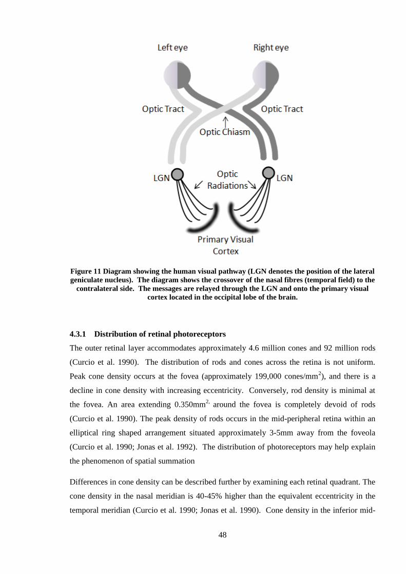
48

Figure 11 Diagram showing the human visual pathway (LGN denotes the position of the lateral

geniculate nucleus). The diagram shows the crossover of the nasal fibres (temporal field) to the

contralateral side. The messages are relayed through the LGN and onto the primary visual

cortex located in the occipital lobe of the brain.

4.3.1 Distribution of retinal photoreceptors

The outer retinal layer accommodates approximately 4.6 million cones and 92 million rods

(Curcio et al. 1990). The distribution of rods and cones across the retina is not uniform.

Peak cone density occurs at the fovea (approximately 199,000 cones/mm2), and there is a

decline in cone density with increasing eccentricity. Conversely, rod density is minimal at

the fovea. An area extending 0.350mm2,

around the fovea is completely devoid of rods

(Curcio et al. 1990). The peak density of rods occurs in the mid-peripheral retina within an

elliptical ring shaped arrangement situated approximately 3-5mm away from the foveola

(Curcio et al. 1990; Jonas et al. 1992). The distribution of photoreceptors may help explain

the phenomenon of spatial summation

Differences in cone density can be described further by examining each retinal quadrant. The

cone density in the nasal meridian is 40-45% higher than the equivalent eccentricity in the

temporal meridian (Curcio et al. 1990; Jonas et al. 1990). Cone density in the inferior mid-

49

peripheral retina has been found to be greater than its superior counterpart (Curcio et al.

1990).

4.3.2 Photoreceptor function in ametropia

Refractive error may affect visual field recordings in several ways: refractive blur can cause

a reduction in light sensitivity, image magnification and minification can lead to inaccurate

recordings, axial length may affect luminance levels.

An increase in myopic refractive error and the concurrent enlargement of the eye, principally

the vitreous chamber depth, have been well documented. The increase in axial length is

believed to cause retinal stretch and subsequently reduced density of retinal cells. Several

studies have reported cone receptor density to be significantly lower in myopia than

emmetropia (Chui et al. 2008; Kitaguchi et al 2007). Cone density is thought to decrease as

a function of increasing axial myopia.

If a mechanical increase in globe size causes reduced density of photoreceptors then it is

possible the photoreceptor cells themselves may be damaged or misaligned. Misalignment is

particularly important as photoreceptor cells are direction specific, i.e. they respond to light

when aligned a specific way only.

4.4 Visual fields and ametropia

Using both automated static perimetry and manual kinetic perimetry a significant loss in

threshold sensitivity for moderate and high levels of axial myopia (-4 to -5D) has been noted

(Martin-Boglind, 1991; Aung et al. 2001; Rudnicka & Edgar 1995; Rudnicka & Edgar

1996). One study, using automated static perimetry, noted deterioration in response at much

lower levels of myopia -2D ±1D (Czepita & Chmielewska 2004).

Increased axial length is closely associated with a higher level of myopia; axial length

greater than 26mm and myopia greater than 5D is reported to be significantly correlated with

a decline in visual field sensitivity (Rudnicka & Edgar, 1995). Decline in the superior

hemifield (inferior retina), particularly the superior temporal field (inferior nasal retina) is

reportedly greater than other quadrants (Rudnicka & Edgar, 1996).

Several explanations have been put forward to explain the visual field sensitivity reduction

in myopia: decreased retinal luminance due to a longer axial length, sensory changes in the

50

photoreceptor cells, decreased photoreceptor density as a consequence of ocular expansion in

myopia (see 4.3.2) (Rudnicka & Edgar, 1995), and misdirection or misalignment of

photoreceptors caused by an increase in axial length hindering their sensitivity to light.

Optic disc tilt is also a commonly reported anomaly noted in myopic individuals; perimetric

studies have shown disc tilt to alter visual field sensitivity by lowering of the mean defect

(the mean deviation between expected ‗normal‘ values and the measured values), (Tay et al.

2005). Of particular interest to the current study is the notion that ocular expansion may

affect visual field sensitivity.

4.5 Summary

Visual field testing provides a measure of visual function. Ocular expansion which is often a

feature of myopia can potentially damage or misdirect retinal cells. Photoreceptor cells are

direction specific; if misaligned their functional ability may be hindered. Additionally,

myopic eyes may display reduced visual field sensitivity due to the longer distance the light

has to travel to reach the retina, increasing the risk of light scatter and absorption by ocular

structures. This thesis will aim to address whether ocular shape is correlated with visual

field sensitivity using the Humphrey Visual Fields Analyser and specific indices of ocular

shape derived from MR imaging.

Further information on the type of perimeter used in this thesis is detailed in section 7.4.

51

5 ELECTROPHYSIOLOGY AND MYOPIA

5.1 Introduction

Electrophysiological testing allows objective measurement of ocular function through

assessment of the retinal electrical responses to a light stimulus. The electrical response from

the eye is received by electrodes, which are attached to the subject; the responses are

amplified and converted to waveforms.

Electrophysiological testing is widely used as a diagnostic tool in ophthalmology, through

several different variants. Two of these variants will be discussed in the context of this

thesis; the electroretinogram (ERG) and the multifocal electroretinogram (mfERG).

5.2 The electroretinogram

The electroretinogram (ERG) tests the accumulative electrical retinal cell response to light.

The test can be manipulated to examine several different retinal cell types. Electrodes are

typically placed on a dormant site such as the forehead, referred to as the reference electrode,

and on the cornea to receive the signal; the active electrode. The potential difference

between the two electrodes is the response (in nV).

The stimuli are presented using the Ganzfeld method to ensure a uniform luminance across

the retina. The patient fixates on a central target, with pupils fully dilated to allow for

maximal response from the peripheral retinal areas. The electrical response is amplified and

displayed as a waveform, which is interpreted with reference to the characteristics of its

amplitude and time course. The response can be contaminated by background electrical

interference, subject blinking, and also by facial muscular action such as jaw clenching;

therefore each reading should be repeated to allow for an average of two readings to be

calculated.

The waveform comprises two components; a negative ‗a‘ wave followed by a positive ‗b‘

wave. The negative ‗a‘ wave response is thought to derive from the hyperpolarisation of the

photoreceptors, and the positive ‗b‘ wave is thought to represent the polarisation of the

Müller and ON-bipolar cells.

52

A weak light stimulus is insufficient to stimulate photoreceptors and produce an ‗a‘ wave, in

such situations only a ‗b‘ wave will be produced. Conversely if the light stimulus is too

bright only an ‗a‘ wave will be produced.

Figure 12 Typical ERG waveform

The amplitudes of the a and b waves are recorded. The time from response onset to the

trough of the a and peak of the b wave, known as the implicit times are also recorded (see

Figure 12).

Although the ERG is still in clinical use today it does have several shortcomings, in

particular its lack of sensitivity to localised focal loss of function. Subsequently

improvements to the design have been made, namely the multifocal ERG.

5.3 The multifocal electroretinogram (mfERG)

In 1992 the multifocal ERG (mfERG) was introduced by Sutter and Tran (1992). The

mfERG allows multiple locations of the retina to be tested simultaneously, providing a

topographical representation of electrical activity. Until the introduction of the mfERG,

ERGs were often used. The main problem with the ERG was the lack of specificity to a

particular area of the retina, and conditions affecting smaller retinal areas could have been

left undetected. The mfERG can be described as an ERG of multiple retinal areas

(depending on the mfERG paradigm used).

53

The mfERG stimulates the central 50 of the retina. Stimuli consist of a series of 61, 103 or

241 hexagons; each one may be thought of as independent stimuli stimulating individual

retinal areas (Hood et al. 2003). The hexagons are response density scaled to account for the

decreasing density of cone cells with increasing eccentricity from the fovea, whereby smaller

hexagons are presented in the central regions and larger hexagons are presented in the

periphery (see Figure 13). Each hexagon flashes either on (white) or off (black), typically

changing every 13.3 milliseconds (Hood 2000). Only half the hexagons are presented at any

one time therefore the mean luminance presented is kept constant. The International Society

for Clinical Electrophysiology in Vision (ISCEV) guidelines suggest luminance levels of the

white hexagons to be between 100-200cd/m² (Marmor et al. 2003). The flashing and non

flashing of the hexagons may appear to occur randomly, however each hexagon is governed

by a pseudo-random binary sequence; an m-sequence. The m sequence assumes two states 0

(no flash), or 1 (flash). At the beginning of a recording each hexagon is in a different phase

of the sequence. Each recording takes 4-7 minutes and is often broken down into 15-30

second segments. Longer test durations are associated with decreased subject compliance

through blinking and losing fixation of the central target. The response from each

presentation is extracted by use of mathematical algorithms to produce an average response

for the respective area stimulated. The responses from many hexagons can be grouped

together to investigate specific retinal regions.

The interval between flashes can be changed to produce different mfERG recording

paradigms. Increasing the interval between flashes produces a waveform response akin to

the full field ERG waveform.

Figure 13 Hexagon stimulus used in mfERG testing (from Marmor et al. ISCEV guidelines

2003)

54

5.3.1 First and second order kernels

The mfERG waveform bears some similarity to an ERG wave, however instead of an ‗a‘ or

‗b‘ waves as with the ERG , the mfERG wave is comprised of positive and negative

components; referred to as P and N respectively.

Figure 14 Typical waveform response from the mfERG (from Marmor et al. ISCEV guidelines,

2003).

The most commonly analysed component of the mfERG is the first order kernel; this is

obtained by adding all the recordings following a flash (white) stimulus, in a particular

hexagon, and subtracting all the recordings following a non flash (black) stimulus, for the

same hexagon. It comprises a negative deflection (N1) followed by a positive peak (P1).

The second order kernel assesses the effect of the preceding stimulus, which may or may not

be a flash stimulus; therefore the second order kernel response is not a true response itself

but a calculation based on the first order kernel (see Figure 14). The cellular origins of the

second order response have been attributed to the inner retina, but evidence is equivocal.

5.3.2 Tools for mfERG analysis

The Visual Evoked Response Imaging System (VERIS) for mfERG recordings has multiple

tools which can facilitate analysis. A widely used tool is the averaging of responses. Spatial

averaging helps reduce noise from each hexagon, smoothing the waveform (Hood et al.

2008). The averaging tool collates the responses for each of the hexagons and divides by the

root mean square. As is the case with all averaging, there is the potential to lose small

changes in response. The Edit groups function within the VERIS program allows

55

calculation of the average response from specific areas e.g. concentric rings, quadrants,

hemifields. The separation into distinct retinal areas is particularly useful for this thesis;

mfERG quadrant responses can be investigated with reference to specific indices of ocular

shape for each retinal quadrant as derived by 3D MR imaging.

The VERIS program also allows 3-dimensional topography maps to be generated, by

dividing the response amplitude by the area of the hexagon (see Figure 15).

Figure 15 3-dimensional topography plot of mfERG response (figure taken from subject data

set, left eye)

5.4 Cellular origins of response

The mfERG response is believed to originate predominately from the bipolar cells with

smaller contributions from the photoreceptor (mainly cone) and amacrine cells. The

contributions from ganglion cells are thought to be minimal or absent (Hiid et al. 2002).

To evaluate the contributions from various cells, studies on rhesus monkeys have shown that

after injection with the chemical tetrodotoxin, TTX, the mfERG response closely resembled

that of a human. Using pharmacological agents to further manipulate responses it was

concluded that the N1 response was derived from the OFF bipolar cells and in general there

56

was only a small contribution from the photoreceptors except in the central 6 where the

contribution is greater. It was also found that the P1 response originated from the

depolarisation of the ON cells and recovery of the OFF cells (Hood et al. 2002). The origin

of the N2 response is still uncertain (Hood et al. 2002). There is thought to be little

contribution from the ganglion cells to the mfERG response (Hood et al. 2003).

The mfERG has been used successfully to diagnose and investigate a multitude of

pathological disorders including retinitis pigmentosa, cone dystrophies, glaucoma and

myopia (Chen et al. 2006a;b).

The diagram below (Figure 16) shows the model developed by Hood et al (2002) outlining

the relative contributions of cells to the mfERG response wave. Damage to, or before, the

bipolar cells would cause reduction of the waveform amplitude, (Hood et al. 2003). Damage

to the ganglion cells (the inner retina) would not cause a reduction in amplitude (see Table

1).

Figure 16 Cellular responses in mfERG (after Hood et al. 2002)

57

Damage to Mechanism P1 (‘b wave of’) mfERG

Amplitude Implicit time

Cone Receptor

Outer segment

damage or cell

loss

Smaller

Smaller

Moderate delay

Normal

Outer plexiform

layer

Altered synaptic

transmission Can be normal or larger Large delay

ON bipolar cells Cell loss Smaller Moderate delay

OFF bipolar

cells Cell loss Larger Slightly faster?

Inner plexiform

layer

Altered synaptic

transmission OR

cell loss

Approx. Normal (waveform

changes)

Small delay

(<3ms)

Ganglion cells Cell loss Approx. Normal Approx. Normal

Table 1 The site of retinal damage and its consequence for the mfERG response waveform

(after Hood, 2002)

5.5 Myopia and electrophysiology findings

A reduction in electrophysiological retinal response with increasing myopia has been

reported. The results appear to be inconsistent in the type of response which is reduced i.e.

amplitudes, implicit times, or both. Furthermore there is some dispute as to whether it is the

level of myopia that causes the reduction or the associated increase in the axial length.

Due to differences in the cellular origins of ERG and mfERG responses the data from each

type of test is only related, not the same. Consequently ERG and mfERG responses must be

considered separately.

5.5.1 Myopia and ERG

A reduction in ERG responses associated with myopia or axial length has been reported

(Blach et al. 1966; Perlman et al. 1984; Westall et al. 2001). Blach et al. (1966) carried out

scotopic ERG recordings (thus eliciting a rod dominated response) on highly myopic

subjects with myopia ranging from -9D to -26D. They found both ‗a‘ and ‗b‘ waves to be

58

affected; a large variation in ERG responses was also noted which they believed to relate to

retinal myopic degenerative changes.

Westall et al. (2001) carried out standard ERGs on 60 young adult subjects, with refractive

errors ranging from +0.75D to -14.50D and axial lengths ranging from 22.2mm to 30.0mm.

They found the implicit times were not affected by either myopia or axial length. A

significant relationship between reduced amplitude and a longer axial length was noted.

Westall et al. suggested that should myopia be of lenticular or corneal origin and not

associated with increased axial length then theoretically ERG response should not be

affected at all.

5.5.2 MfERG and myopia

Kawabata and chi-Usami (1997), examined the first order kernel responses on thirty young

adult subjects (mean age 26.1 years). The subjects were placed into one of three groups

according to refractive error: emmetropia/low myopia (MSE ± sd = -0.78±0.89D), medium

myopia (-4.30±0.81D), and high myopia (-10.33±3.38D). The purpose of the investigation

was to evaluate functional changes in myopic eyes. Myopia was believed to be principally

of axial origin and not corneal or lenticular. In addition to the more typical mfERG analysis,

examining all traces and concentric ring averages, the readings were also divided into

quadrants: superior temporal, superior nasal, inferior temporal and inferior nasal (see Figure

18).

Figure 17 Diagrammatical representation of the concentric ring averages analysed, note ring 1

denotes the presumed foveal response.

59

Figure 18 Diagrammatical representation of the quadrant average analysis undertaken by

Kawabata and chi-Usami 1997. N.B the horizontal and vertical meridians have been omitted,

presumably to ensure equal hexagonal responses from each quadrant and also to exclude the

optic nerve head

Results showed a decrease in amplitude and an increase in implicit times as myopia

increased; N1 amplitudes r=0.713, and for P1 r=0.772, p=<0.0001 for both cases. Implicit

times increased with greater levels of myopia: the first latency r=0.603 p=<0.0004, and the

second r=0.731 p=<0.0001. Amplitudes from the peripheral regions were affected to a

greater degree than central regions. Implicit times were delayed more in the inferior regions

than superior. Kawabata and chi-Usami (1997) concluded that a reduction in cone cell

function in myopia was responsible for the reduced responses noted through mfERG testing.

In a separate study looking at ring responses (Chan and Mohidin, 2003), first order response

amplitudes were reportedly affected by increasing axial length, as were paracentral (ring 3)

responses. Second order response amplitudes were not affected in the central region,

however, the paracentral and peripheral regions showed a reduction in amplitude with

increasing axial length (rings 2 to 5). Overall the average of the responses measured showed

a decrease in amplitude of 6-10% with every 1mm increase in axial length.

The central response amplitude (P1) originates from the photoreceptors and Chan and

Mohidin (2003) suggested the reduced amplitude may relate to central retinal stretch. The

first slice of the second order response waveform is believed to originate from the outer

plexiform layer (Hood, 2000) and Chan and Mohidin believed that this somehow attributed

to the paracentral deterioration in responses.

60

To elicit whether the main contributory factor to reduced mfERG responses is myopia or

axial length Chen et al. (2006) carried out a series of mfERG studies using various recording

paradigms. In a group of 30 young adult subjects P1 amplitudes and implicit times of

standard mfERG recordings were examined with respect to their axial lengths and refractive

error. Subjects comprised of 10 emmetropes and 20 myopes, myopic subjects were further

classified into stable or progressing myopes. Refractive error ranged from plano to -9.75D.

Using ANCOVA statistical analysis the authors accounted for axial length as a covariate of

myopia and vice versa. A longer axial length correlated with a longer implicit time and a

refractive group effect was also noted. The myopic group was noted to have a longer

implicit time of 1.3-3.1ms compared with the emmetropic controls, and as noted by

Kawabata and chi-Usami. the delays were greatest in the periphery. Notably, Chen et al.

(2006) reported statistical differences between the emmetropic and progressing myopia

groups only. 15% of the variance in implicit time results was explained through axial length,

27% by refractive error and the remaining believed to be due to inter subject variability.

Unlike previous investigations, a detrimental effect of myopia or increased axial length was

not noted for the response amplitude.

Further work by the same group using different mfERG recording paradigms has led to the

suggestion that the changes are a consequence of myopia and not a precipitating factor of

myopia (Chen et al. 2006a;b;c;d). Additionally, the authors found the responses which

originated from photoreceptors were not affected by myopia. Most recently, the group has

examined oscillatory potentials of mfERG recordings and noted significant differences

between stable and progressing myopes (Chen et al. 2006b), which is suggestive of inner

retinal contributions to myopic development.

In children mfERG changes (using standard paradigms) have been shown to correlate with

greater myopic progression (Luu et al. 2007).

In summary, changes in mfERG readings suggest a greater level of myopia or axial length

may produce reduced amplitudes and/or longer implicit times. From previous work

examining mfERG responses in adults, it can be hypothesised that the outer retinal layers are

affected by myopia, but it is the inner retinal layers which may precipitate myopia.

61

5.5.3 Reasons for reduced electrical response in myopia

Ocular resistance

Perlman found an inverse relationship between the b wave response of an ERG and a longer

axial length (Perlman et al. 1984). It was believed that increased ocular resistance, that is

resistance to the electrical signal by ocular tissues and structures, caused the reduction in

ERG response. Perlman believed resistance was more likely to reduce the signal than

reduced sampling density or reduced receptor function although a number of studies have

disagreed with this proposal (Chen et al. 2006; Kawabata & chi-Usami 1997).

Eye size and shape

Westall et al. 2001 suggest that the increase in axial length and not the level of myopia, acts

as a causative factor for reduced ERG responses. The group postulated that myopia of

lenticular or corneal origin would not produce differences in ERG responses (Westall et al.

2001). Chan and Mohidin examined the link between axial length and the mfERG and also

attributed the reduction in responses to morphological changes associated with increased

axial length.

Furthermore, there is a proposal that the retinal cells of highly myopic eyes may be either

inherently dissimilar to emmetropic eyes or different as a consequence of myopic damage

(Chen et al. 1992). Kawabata and chi-Usami believed the reduction in mfERG responses

with myopia was due to cone loss, possibly associated with ocular expansion.

Dopamine

Dopamine in the human eye is produced in specific amacrine cells within the retina. The

role of dopamine is multiplex, it is involved in accommodation, blink rate, iris aperture

control and ganglion cell activity (Yeung et al.2001; Spiers, 1969). Recently, it has been

suggested that perhaps altered levels of dopamine may influence the human mfERG

response (Chen et al. 2006a). Through work conducted largely on animals, depleted levels

of the hormone dopamine have been noted in cases of induced myopia (McCarthy et al.

2007). A recent study of myopic development in children noted that sunlight aided the

production of dopamine, and reported that although dopamine levels were not measured in

the subject group, lower myopic refractive error was noted in children who spent more time

outdoors (Rose et al. 2008).

62

5.6 Summary

Electrophysiological testing provides an objective measure of ocular function. The ERG

test provides a generalised summed response of ocular function, whilst the mfERG provides

a topographical representation of ocular functions. Previous studies have identified reduced

responses in both ERG and mfERG with either longer axial length or higher refractive levels

of myopia. The effects of higher refractive levels of myopia and axial length are difficult to

differentiate as they invariably correlate.

There are many possible explanations for reduced electrical responses in myopic or longer

eyes. Often decreased retinal cell density as a result of retinal myopic stretch is attributed

with the reduction in response. Many studies have identified loss in paracentral and

peripheral regions, whereas others have noted losses to be more central. Thus far most

studies have relied upon axial length as a measure of eye size, however this technique is

limited. Axial length alone does not indicate eye shape and so is only useful if considering

the central hexagon response. The recent development of 3-dimensional ocular MRI enables

the comparisons between mfERG responses and individual ocular shape. The findings of

this study would help answer the question of whether it is myopia or eye shape that causes

the reduction in mfERG response. The thesis addresses correlations of mfERG testing and

ocular shape in Chapter 13.

63

6 GANGLION CELL DENSITY AND OCULAR SHAPE

6.1 Introduction

Ganglion cells reside in the ganglion cell layer in close proximity to the inner retina. The

primary function of ganglion cells is the transmission of information as action potentials

between the photoreceptors, via horizontal, bipolar and amacrine cells, to the rest of the

visual pathway. Ganglion cell axons form the optic nerve, which projects to the occipital

cerebral region, specifically the visual cortex.

A single ganglion cell can receive and transmit data from numerous photoreceptors; this

process is termed convergence. The ratio of retinal ganglion cells to cone cells in the central

foveal region is approximately 2; this ratio declines to approximately 0.5 for retinal regions

beyond the central 19º around the fovea, thus there is a greater need for convergence in the

peripheral retina (Sjöstrand et al. 1999). The convergence process helps balance the spatial

resolution required to detect objects peripherally while still retaining the high level of

resolution required to distinguish finer details of objects in the central field. Without

convergence a greater number of ganglion cells would be necessary to transmit information

to the visual cortex, thus the need for a larger optic nerve head which would in turn produce

an intolerably large blind spot in the visual field.

6.2 Distribution of ganglion cells

There are approximately 32000-38000 ganglion cells per mm2 in the retina; their distribution

across the retina is non homogenous (Curcio & Allen 1990; Hebel & Hollander 1983). The

cells are arranged in an elliptical ring shape surrounding the fovea, (Curcio et al. 1990).

Quadrantic differences in the distribution of ganglion cells have also been noted; a

histological study reported nasal density to be 300% greater than that of the temporal retina.

The same study noted a greater density of ganglion cells in the superior retina by 60%

compared to that of the inferior retina (Curcio et al. 1990). In addition to histological

studies, ganglion cell density in humans may also be inferred from psychophysical

techniques (Anderson et al. 1992; Anderson et al. 1995; Chui et al. 2008).

64

6.3 Receptive fields

All retinal ganglion cells have a base firing rate which describes the level of spontaneous

discharge from the cell in the absence of stimulation. Stimulation in the form of photons

(units of light) can increase or decrease the firing rate of the cell.

Studies on mammalian retina, mainly cats, have shown ganglion cells to possess non

homogenous circular receptive fields. Two zones arranged in concentric circles have been

identified, each with their own stimulation and response characteristics. Stimulation of the

central zone has been found to elicit a separate and opposite response to the stimulation of

the periphery. A central excitatory region surrounded by a peripheral inhibitory ring is

termed an on-centre cell; conversely, a cell with a central inhibitory and peripheral excitatory

configuration is termed an off-centre cell (Kuffler, 1953).

The notion of concentric receptive fields in ganglion cells was explored further by use of

sinusoidal grating stimuli (Enroth-Cugell & Robson 1966). Two further cell subtypes were

identified; X and Y cells. X cell responses were found to increase when an on-centre cell

was exposed to light stimuli in the central ring and dark stimuli in the peripheral ring (Figure

19). When the central stimulus was darker than the peripheral, a decline in response was

shown. If the sinusoidal grating was positioned to produce a similar stimulus at both the

centre and periphery there was no change in the cells response. The X cells were said to

show linear spatial summation. Conversely, Y cells responded at the onset of stimulus; the

response was unrelated to the stimulus sinusoidal grating phase.

Figure 19 On-centre ganglion cells and sinusoidal grating

The X cell response varied with sinusoidal grating phase changes and therefore responded to

motion. Y cells, did not respond to movement. It should be noted that the size of ganglion

65

cell receptive fields is not uniform across the retina; cells located peripherally have larger

receptive fields than those located centrally.

6.3.1 Magnocellular and Parvocellular cells

Receptive fields in primate retinal ganglion cells follow a similar structure to X and Y cells

found in cats. The primate ganglion cells can be broadly divided into two groups;

Magnocellular (M) and Parvocellular (P), the names correspond to the cerebral streams

followed by each cell type. Although primate ganglion cells resemble cat ganglion cells in

many ways, their distribution and properties vary.

Each concentric region of the P cell receptive field possesses an affinity for a particular

wavelength of light (De Monasterio & Gouras 1975). This characteristic response to colour

is known as colour opponency. Conversely, M cells do not display colour opponency

therefore they are often referred to as ‗broadband‘ cells,

Earlier studies indicated that M cells showed the ability to respond to motion; however,

recent work on humans has demonstrated that P cells can also detect motion at specific

retinal eccentricities (Anderson et al. 1995; Galvin et al. 1996).

Further characteristics of M and P cells are listed in Table 2

M cells P cells

Thicker axons Thinner axons

Phasic/transient response Sustained/tonic response

Large cells Small cells

Broadband Colour opponency properties

Higher contrast sensitivity Lower contrast sensitivity

Larger receptive fields with increasing eccentricity from the fovea

Table 2 Magno- and Parvocellular differences

66

In addition to M and P cells, a third group of ganglion cells, known as K cells (or

Koniocellular, originally termed ‗rarely encountered cells‘) have been found in primates

(Schiller & Malpeli 1977). K cells also display non-linear spatial summation characteristics

similar to M cells but at a much slower conduction velocity.

6.4 Sampling theorem, aliasing and the Nyquist limit

In vivo ganglion cell sampling through psychophysical methods exploit the on/off centre

arrangement of ganglion cell receptive fields and the sampling theorem. The sampling

theorem can be used to describe the limitations placed upon the visual system by the

sampling frequency. Assuming ganglion cells are regularly distributed in a given retinal

region, the sampling theorem dictates that for a sinusoidal grating to be detected in order to

reconstruct the signal accurately, a minimum of two sampling points per cycle are required

i.e. one sampling point for the peak of the wave and one for the trough. The limit of the

sampling frequency is referred to as the Nyquist limit. If performance falls below the

Nyquist limit, (when responses are correct less than 50% of the time); this would produce

aliasing or misrepresentation of the signal. In the central foveal region visual optics act as a

filter to limit frequencies outside the limits of the bandwidth imposed by the distribution of

the foveal cones, to prevent aliasing. High spatial frequency laser interference fringes are

independent of the eye‘s optics and can be used to induce foveal aliasing.

6.5 Peripheral visual function

Beyond the foveal region, cone density cannot be relied upon to indicate potential visual

acuity due to the decline in cone receptors and the increased amount of signal convergence

that takes place. Hence, ganglion cell density is of particular interest in the peripheral retinal

regions.

The neural limitations placed upon the visual system in the peripheral retina by ganglion

cells are believed to be directly associated with reduced visual resolution (Thibos et al.

1987). However, other factors may also play a role in image degradation: the presence of

peripheral aberrations, stimulus contrast and correction of peripheral refractive error.

A study using histological samples found beyond 11-20º eccentricity from the fovea, the

relationship between minimum angle of resolution (MAR), receptive fields and retinal

ganglion cells to be non linear. The non linearity has been explained by the lack of

67

differentiation between ganglion cell subtypes in sampling studies (Sjöstrand et al. 1999).

Conversely, other studies have noted the relationship of ganglion cell density and visual

resolution to be well correlated (Anderson et al. 1992). One study determined ganglion cell

density by use of psychophysical techniques in several different retinal locations referencing

findings to previously published histological data (Anderson et al. 1992; Curcio & Allen

1990). At an eccentricity of 25˚, the greatest resolution acuity was found to be in the nasal

quadrant (see Figure 20). This finding correlates well with the increased density of ganglion

cells noted in this region (Curcio et al. 1990). Nasal-temporal asymmetries in sensitivity had

previously been noted by Anderson et al. (1991); at eccentricities of 25-55° the nasal retina

was shown to be more sensitive than the temporal. Investigations of the vertical meridian

(examining superior-inferior asymmetries) did not find such hemifield differences.

Figure 20 Visual resolution limit in cycles per degree at an eccentricity of 25˚, at radial

locations around the retina (Anderson et al. 1992)

6.6 Myopia, eye size and peripheral ganglion cell function

Of particular interest to the current study is the evidence showing the peripheral retina to be

structurally dissimilar between different refractive groups (Atchsion et al. 2005). In myopia

as the globe expands concurrent retinal expansion and subsequently retinal stretch is

believed to take place (Vera-Diaz et al. 2005). As a consequence, retinal receptors may be

68

misaligned, misdirected, damaged, or decreased in density. Investigation of ganglion cell

density in myopic subjects may therefore help clarify the effects of shape and refractive error

on peripheral retinal function.

Specifically, ganglion cell density has been found to be reduced in myopes (Chui et al. 2002)

and consequently visual resolution believed to be sampling limited (Chui et al. 2005) in

direct proportion to the number of ganglion cells (Popovic & Sjöstrand 2005).

One study investigating aliasing at the fovea estimated the Nyquist limit of an emmetropic

eye to be 56 cycles per degree (expressed in object space/visual field); the value was

calculated by assuming that firstly the maximum foveal proximity of cone receptors is 3µm

and secondly that 1° of retina corresponds to 0.29mm. Using this value, a prediction may be

made regarding the potential effects of myopia on retinal spacing and thus sampling limits.

Strang et al. (1998) proposed three models of myopic growth; equatorial stretch, global

stretch and posterior pole stretch (see Figure 21).

Figure 21 (a) Equatorial stretching (b) Global expansion (c) Posterior Pole (after Strang et al.

1998)

Strang et al. made predictions of resolution ability with reference to each myopic model

(Strang et al. 1998). The predictions were based upon the parameters set by Williams et al.

(Williams, 1985). Eyes which followed the equatorial stretch model were expected to have

optical rather than neural limitations affecting the resolution. For the posterior pole stretch

model, neural resolution was predicted to fall at approximately 5D of myopia, and in the

global expansion model resolution was predicted to fall beyond 15D of myopia (see Figure

22). Thirty-four subjects with refractive errors ranging from plano to -14D were examined.

The predictions were not confirmed by their findings. This may be due to the models being

overly simplistic as it is likely that subjects‘ eyes were a combination of two or more of the

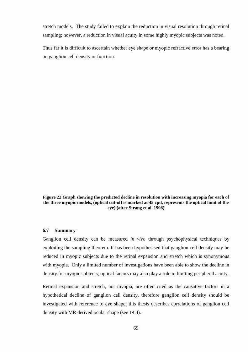
69

stretch models. The study failed to explain the reduction in visual resolution through retinal

sampling; however, a reduction in visual acuity in some highly myopic subjects was noted.

Thus far it is difficult to ascertain whether eye shape or myopic refractive error has a bearing

on ganglion cell density or function.

Figure 22 Graph showing the predicted decline in resolution with increasing myopia for each of

the three myopic models, (optical cut-off is marked at 45 cpd, represents the optical limit of the

eye) (after Strang et al. 1998)

6.7 Summary

Ganglion cell density can be measured in vivo through psychophysical techniques by

exploiting the sampling theorem. It has been hypothesised that ganglion cell density may be

reduced in myopic subjects due to the retinal expansion and stretch which is synonymous

with myopia. Only a limited number of investigations have been able to show the decline in

density for myopic subjects; optical factors may also play a role in limiting peripheral acuity.

Retinal expansion and stretch, not myopia, are often cited as the causative factors in a

hypothetical decline of ganglion cell density, therefore ganglion cell density should be

investigated with reference to eye shape; this thesis describes correlations of ganglion cell

density with MR derived ocular shape (see 14.4).

70

7 INSTRUMENTATION

7.1 Introduction

Approximately 17 subjects for the MRI study had been recruited prior to October 2006

(before the PhD studentship began); for the majority of these subjects a range of ocular

biometry measurements were obtained by Dr Nicola Logan, Professor Bernard Gilmartin,

Professor Krish Singh and Elizabeth Wilkinson.

Subjects were recruited predominantly from the Optometry undergraduate and postgraduate

programs at Aston University. A total of 76 subjects were scanned however only 73 are

included in the main data set; subjects with refractive error greater than 15D were excluded

from general analyses. Ages for the main subject data set ranged from 18 years to 40 years.

Subjects were predominantly of White or British Asian ethnicities. Ethical approval was

acquired for all experiments and informed consent obtained from subjects.

The range of data collection comprised MR scanning, ocular biometric measures using the

Zeiss IOL Master and Oculus Pentacam, visual fields testing with the Humphrey Visual

Fields Analyser, multifocal ERG VERIS recordings, ganglion cell density, peripheral

refraction measurements with the Shin Nippon autorefractor, and the issuing of a

questionnaire.

7.2 Shin Nippon Autorefractor

The Shin Nippon SRW 5000 (Japan) is a wide field binocular open view IR autorefractor

allowing objective measurement of refractive error. The instrument has been used widely in

research (Chat & Edwards, 2001; Logan et al. 2005).

Refractive readings by the S-N SRW 5000 have shown high repeatability and high validity

which have been established through correlations with subjective refraction in both adults

(Mallen et al. 2001) and children (Chat & Edwards 2001).

The subject is positioned by use of an adjustable chin and fixed head rest. The practitioner is

able to view the anterior eye on a small black and white monitor, and through use of a

joystick can align and focus the centre of a ring shaped (necklace) mire with the eye. To

obtain a reading a minimum pupil size of 2.9mm is recommended by the manufacturer.

71

Once the subjects‘ eye is aligned, the practitioner presses the release button in order to take a

measurement. Results may be printed and stored; the option to produce electronic copies

through connection to a computer also exists, however, this method was not used in the

present study.

The instrument is able to measure a wide range of refractive errors; ±22D spherical

component and ±10D cylindrical component. The values are given to the nearest 0.125D

and the cylindrical axis expressed in 1˚ increments.

Shin Nippon autorefractors have been used to study accommodation and peripheral

refraction. The extensive use of the Shin Nippon range for peripheral refraction has been

reviewed (Fedtke et al. 2009) and compared to other techniques and is cited as the principal

instrument of choice.

In order to take peripheral refraction measurements with an autorefractor the presentation of

the target normally requires a degree of modification. In the current study an attachment was

fitted to the Shin Nippon autorefractor casing; the attachment was marked at 5˚ intervals up

to a maximum of 30˚ right and left from the visual axis (0˚). The peripheral refraction

attachment had been made for previous studies using the Shin Nippon by Dr Leon Davies

and Dr Edward Mallen; a fixation target was attached to the autorefractor arm at a viewing

distance of 1m.

Prior to obtaining autorefraction readings all subjects were dilated with 1% tropicamide

ophthalmic solution (Minims®, Bausch and Lomb, Surrey, U.K); this ensured maximum

pupil size which enabled the acquisition of more peripheral measurements, additionally

tropicamide induced a cycloplegic effect which helped to minimise any active

accommodation. Prior to the instillation of tropicamide intra-ocular pressure (IOP) readings

were obtained using standard commercially available non-contact tonometers, IOP readings

were repeated post dilation and advice on possible adverse effects of tropicamide was given.

7.3 Zeiss IOL Master

The Zeiss IOL Master is a non-contact device used for measuring ocular biometric

parameters. Measurements possible include axial length, corneal radii, anterior chamber

depth, and horizontal iris diameter. The IOL Master is used extensively in hospitals for

calculation of the required intraocular lens power pre cataract surgery.

72

The operation of the IOL Master is much like that of an autorefractor; the subject rests

his/her head on the head rest and chin on the adjustable chin rest. The subject fixates upon a

target located within the instrument, the practitioner then uses the joystick to adjust the

positioning of the unit and focus the mires. Each type of measurement requires the

refocusing and realignment of mires, i.e. there are separate sets of mires for keratometry,

axial length and anterior chamber depth.

Axial length measurements

The IOL Master measures axial length through an adaptation of partial coherence

interferometry. A Michelson interferometer splits an infra red light beam (λ =780nm) into a

dual beam comprising two partial beams (which reduces any longitudinal eye movements

affecting the recording). On entering the eye the dual beam is reflected at two surfaces; the

anterior corneal surface and the pigment epithelium. If the path between the partial beams is

smaller than the coherence length; an interference signal is detected, (Drexler et al. 1998;

Goel et al. 2004). This condition is met through the movement of one of the mirrors within

the system. The interference is detected by a photodetector and measured relative to its

positioning from the interferometer mirror.

Prior to the introduction of the IOL Master axial length measurements were predominantly

taken using A-Scan ultrasound. A distinct disadvantage of ultrasound biometry is the higher

likelihood of cross infection between subjects owing to the use of a contact probe.

Keratometry

Keratometry is the measurement of the corneal radius of curvature and readings can be used

to estimate the degree of corneal cylindrical error. The measurements obtained through the

IOL Master are comparable to those made by commercially available instruments used in

clinical practice, such as the Javal-Schiotz keratometer (Santadomingo et al. 2002; Nemeth

et al. 2003).

Anterior Chamber Depth (ACD)

The anterior chamber depth describes the distance along the optic axis from the posterior

corneal surface to the anterior crystalline lens surface. The repeatability of ACD

measurements with the IOL Master have been queried (Lam et al. 2001). Furthermore

comparison of ACD measurements from the IOL Master with other commercially available

instruments have found equivocal results, with some studies reporting comparable results

73

between instruments (Lackner et al. 2005) and others finding significant differences

(Hashemi et al. 2005).

In summary, previous reports suggest that the Zeiss IOL Master has good repeatability, for

keratometry and axial length measurements, and is a valid instrument of choice for a range

of ocular biometric measurement. Results are not, however, interchangeable with those from

other ocular biometric instruments.

7.4 Zeiss Humphrey Visual Fields Analyser

The Zeiss Humphrey Visual Fields Analyser (HVFA) is a well established and widely used

automated perimeter in both research and clinical settings; it is generally accepted as the

gold standard instrument for automated visual fields testing. In clinical settings the HVFA is

often recommended for use in glaucoma patients, i.e. individuals who may have subtle visual

field changes.

During the test subject ametropia is fully corrected by use of full aperture trial lenses or by

contact lenses. Subjects are positioned by use of adjustable chin and forehead rests, and are

required to fixate on a target inside the perimeter bowl.

A push switch is given to a subject, which during the test the subject uses to indicate the

presence of a stimulus. The stimulus for most HVFA programs is target size III (4mm²);

however other sizes may be used to detect more subtle or gross defects. The stimulus will

vary in intensity; from 0.8 to 10,000 apostilb (asb), in order to determine the minimum light

detected by the subject; known as the differential light threshold. The background

luminance within the perimeter will however stay constant at 31.5 asb (Wani et al 2005).

As mentioned previously, the HVFA has extensive software to run various different types of

visual field tests. Each test may differ from another by the area of the field covered, number

of points tested, or by the way in which the light threshold is determined. The HFVA allows

use of the Swedish Interactive Threshold Algorithm (SITA) to determine threshold values.

The use of SITA reduces the test time which helps reduce the effect of fatigue associated

with longer testing times, thus producing more reliable results.

There are several types of SITA tests; SITA Standard, SITA Fast and FASTPAC. SITA

Standard is often used as a replacement for full threshold fields as it is faster and shown to

have good repeatability (Chandra et al. 2000). The HVFA provides several reliability

74

indices as a measure of how valid the test is, these include: fixation losses, false positives

and false negatives, (see section 4.2.1).

The Humphrey Visual Field Analyser provides reliable measurements of light sensitivity for

the central visual field. In myopic individuals these measurements are a valuable source of

information as they can provide information about subtle functional changes. Although

studies of automated visual fields in myopia have been previously reported, the approach

taken by the current study is unique as it investigates the previously unreported relationship

between ocular shape and visual field sensitivity.

7.5 Oculus Pentacam

The Oculus Pentacam (Oculus Optikgeräte GmbH, Wetzlar, Germany) is a relatively new

device; it was introduced approximately five years ago. The Pentacam is able to take

numerous measurements of the anterior eye, in particular measurements of the cornea (see

Figure 23). The Pentacam provides a vast amount of information: corneal pachymetry,

corneal volume, higher order aberration maps, and refractive power topographies. The

Pentacam is reported to have high repeatability in particular for pachymetry measurements

(Khoramnia et al. 2007). The use of the Pentacam has been widely advocated by refractive

surgery clinics and hospital services alike.

75

Figure 23 An example of a Pentacam output. The output shows the corneal thickness for an

emmetropic subject (MSE: +0.50D). Further outputs are given for parameters such as corneal

curvature and aberrations.

The instrument uses a rotating slit beam camera which is based upon the Scheimpflug

principle to take measurements at 25,000 locations within the anterior eye. The Scheimpflug

principle describes the relationship between the image plane, object plane and the orientation

of the camera lens, required to achieve a focused cross sectional image.

7.6 Magnetic Resonance Imaging (MRI)

Magnetic Resonance Imaging, MRI, is a method of imaging used to examine soft internal

tissues in humans. MRI is widely used in the field of neurology. The technique works on

the basis of an extremely strong magnetic field and exploits the properties on hydrogen

atoms which are abundant in the human body. The responses from the magnetic fields are

detected by radio waves which are then presented as images.

In the present study a Siemens 3-tesla (Siemens, Erlangen, Germany) whole body scanner

was used to scan both eyes. The MRI scanning protocol allowed images to be obtained in

five minutes and forty seconds (Singh et al. 2006). To explain how the MRI works it is

essential to understand some of the associated background physics.

76

An atom is a structure constituting a central nucleus which contains both positively charged

protons, and neutrons which do not have an electrical charge. The nucleus is surrounded by

negatively charged electrons (Westbrook and Kaut, 2003). The atom is electrically stable if

the number of protons and electrons is equal. If there is a surplus of either, the atom is

electrically unstable and termed an ion.

There are three types of movement within the atom; electrons spinning on their own axis;

electrons orbiting the nucleus; and most important for MRI is the spinning of the nucleus on

its own axis (Bharatah, 2009). The nucleus of biological tissues contains specific MR

sensitive nuclei; these are hydrogen atoms. In general the protons in the hydrogen atom

nuclei are randomly aligned. In the presence of a strong magnetic field, such as that

introduced by the MR scanner, the orientation of the protons is aligned with the new

magnetic field. The protons generally spin around their own axis, however, in the presence

of the strong magnetic field they also spin in a rotary pattern about their own axis know as

the precessional path. The speed at which this path is followed is known as the precessional

frequency, also referred to as the Larmor frequency as it is governed by the Larmor equation

(Westbrook and Kaut, 2003). The precessional frequency of hydrogen varies with different

magnetic field strengths; a higher field strength of 1.5 tesla would produce a greater

frequency than 1.0 tesla.

A pulse of radio frequency waves is applied at the precessional frequency; this causes

resonance to occur. The protons gain energy and their orientation is changed, the magnitude

of change is termed the flip angle and is usually 90° i.e. the opposite direction to the

magnetic field. The radio frequency receiver coil detects the changes in the magnetic field

and is able to record from this the MR signal. The receiver coil may be a small localised coil

e.g. an ocular coil, or a larger full body coil. A localised coil will provide a higher signal to

noise ratio. In this particular study an eight channel phased array head coil was used.

As the radio frequency waves are removed, the energy of the protons is diminished until they

realign orientation with the magnetic fields. The loss of radio frequency emitted is termed

T1 or T2 decay (Westbrook and Kaut, 2003). T2 weighted images were used in the present

study as they optimise organs that are predominantly water based, such as the eye. Each MR

slice had a thickness of 1mm and voxel size was 1.0 x 1.0 x 1.0mm. An earlier protocol

used 0.5 x 0.5 x 1.0mm voxels (Singh et al. 2006). Further details of how the images were

processed and analysed are provided in Chapter 9.

77

As the MR scanner is the centre of a strong magnetic field it is critical that all metallic

objects are removed from the room and from the subjects. In depth screening takes place

prior to any scan, and subjects must speak to the radiographer before the procedure.

The scanner comprises a tunnel like chamber and is accessed by the subject through lying on

a sliding table. In the current study subjects were asked to fixate on a distant LED target

during scans. The images are prone to artefacts therefore movement of the eyes, and other

general bodily movement, can cause blurring of the images.

Inside the scanner the environment can be quite noisy owing to changes in the magnetic field

strength; referred to as gradients (McRobbie et al. 2003). Ear plugs were provided for all

subjects to reduce the loud audio effects of the MR scanner.

7.7 Summary

A number of different techniques are used to assess ocular shape and function as part of the

experiments which comprise this thesis. The high validity and repeatability of each

instrument or technique has previously been reported, therefore no studies of repeatability or

validity have been carried out. Calibration of all lab instruments was maintained throughout

the study.

78

8 SUMMARY OF AIMS AND OBJECTIVES

The principal aim of this thesis is to evaluate the relationship between ocular shape and

visual function.

Several reports demonstrating reduced visual function in myopia have suggested increased

ocular size as a possible causative factor. The increase in ocular size is thought to cause a

concurrent decrease in retinal receptor density and subsequently lead to impaired visual

function (Chen et al. 2006; Chui et al. 2005). Previously limitations in ocular shape imaging

restricted the testing of this hypothesis. Since the introduction of 3-dimensional MR imaging

a more comprehensive model of eye shape may be constructed and subsequently correlated

with tests of visual function (Singh et al. 2006).

3-dimensional ocular MR imaging allows shape parameters from specific areas of the eye to

be evaluated; it is envisaged that evaluations of shape and function will be drawn from

specific retinal quartiles. Tests of visual function will include visual field sensitivity testing,

multifocal electroretinogram testing, and estimates of ganglion cell density. Previously these

tests of have demonstrated reduced responses in myopic eyes.

In order to further evaluate ocular structural aspects, a comparison between peripheral

refraction based retinal contours and MRI based retinal contours is envisaged. As peripheral

refraction is a more accessible and more widely used technique than 3-dimensional ocular

MRI, it is of particular interest to determine whether these two techniques produce

comparable and interchangeable results.

Based on previous literature, it is hypothesised that a detrimental effect on visual function

will be correlated with the increase in ocular size which is synonymous with myopia.

79

9 DEPICTION OF OCULAR SHAPE AS DERIVED FROM 3-DIMENSIONAL

MAGNETIC RESONANCE IMAGING (MRI)

9.1 Introduction

In vivo ocular imaging has proven to be problematic for investigators owing to both optical

and anatomical constraints. Two of the most widely used techniques in recent years have

been peripheral refraction and 2-dimensional MRI (Atchison et al. 2004; 2005; Logan et al.

2004). Both these methods suffer from relatively large areas of the retina being inaccessible

for measurement, and thus assumptions of eye shape in those areas have been made.

Peripheral refraction measurements are usually taken over the central 30-40° at 5° intervals;

thus not accounting for data from approximately 57% of the area examined. Peripheral

refractive studies generally focus on the horizontal meridian; there is limited data for the

vertical meridian. Due to difficulties in measurements, information regarding the oblique

meridians is rarely acquired. Thus information is missed due to large measurement angles

and is also limited to a maximum of two meridians. Furthermore, aberrations created by the

eye‘s optics limit the validity of more peripheral readings. Conversely MRI measurements

are independent of the eyes optics; additionally MRI is not limited by pupil size, allowing

measurements of the whole eye. Until recently all ocular MRI work was limited to 2-

dimensional (2D) methods (Atchison et al. 2005; 2004). Measurements of the height, width

and length of the eye were made using MR data (Cheng et al. 1992; Atchison et al. 2004;

2005). Although 2D MR data can provide valuable information on eye size, it has failed

accurately to quantify the changes in ocular shape. 2D MR imaging is limited by a number

of factors; namely the image slice sizes and methods of data analysis. Despite their relative

limitations both techniques, peripheral refraction and MRI, appear to produce similar results;

reporting myopic eyes to be relatively prolate or less oblate in the posterior retinal regions

compared to emmetropes and hyperopes who tend to be more oblate. 3-dimensional ocular

MR imaging bears many advantages over the 2D method. 3D MRI can provide a more

comprehensive data set providing information on ocular shape, retinal contour, ocular

volume and help to model the shape characteristics of each retinal quadrant.

9.2 3 Dimensional MRI

The acquisition of the MR data is described in more detail in the Instrumentation chapter. In

brief, subjects are required meet a strict set of criteria before consideration for MR imaging.

80

Information regarding the procedure, the prerequisites to scanning, and the possible adverse

effects, was supplied through both written and verbal formats prior to scanning. In the

current study the information sheets, one of which was an exclusion criteria questionnaire,

were read again on the day of the scan. Before committing to the experiment, subjects were

briefed again by the registered radiographer present and any positive responses on the

questionnaire discussed; positive responses may be regarding issues such as dental work or

tattoos. Prior to entering the scanning room all metallic objects were removed from the

subjects due to the strong magnetic fields within the room; subjects were asked to either

change into hospital gowns or bring a change of clothing which was free of metallic zips and

buttons to wear during the procedure. Subjects were then provided with ear plugs to reduce

the noise of the scanner before scanning began.

The scan required the subject to assume a supine position on a stretcher bed inside the

scanner (see Figure 24). Subjects were asked to fixate on a distant red LED target (located

in the MR control room) through use of an inclined mirror system, this target helped to

minimise eye movements which could lead to poor MR images.

The scan itself lasts approximately 5 minutes and 40 seconds with an additional 5-10

minutes to set up the subjects and to give the subjects breaks. Throughout the procedure

subjects were able to communicate with the radiographer via a two way intercom system.

Figure 24 The MR scanner and head coil (c/o Aston University Day Hospital)

81

Post scanning, a set of Digital Imaging and Communications in Medicine (DICOM) files

were generated. DICOM MRI files were converted to image files through use of PC based

software MRIcro. These image files were then accessed using MAC based freeware

software mri3dX.

Mri3dX

The Mri3dX program shows images in three planes; coronal, axial and sagittal. The program

allows the user to proceed successively through the image slices, while simultaneously

viewing images in the three plane formats (see Figure 25).

The images generated were optimised to show the fluid filled chambers of the eyes at much

higher contrast than the surrounding bony orbit (Gilmartin et al. 2008). In the 3D ocular

imaging technique images of the two eyes are shaded with 1mm³ voxels, through use of a

flood-filling algorithm. There is a considerable amount of overspill with the automatic

shading function therefore manual manipulation is required. Shading manipulation requires

careful examination of each MR image slice and it must be ensured that shading is contained

within the ocular regions only; any overspill is subsequently corrected. The image slices are

1mm in thickness, therefore there are approximately the same number of slices as

millimetres of axial length. Separate shades are used for the right and left eyes to help

differentiate the data.

Figure 25 The three different views presented in mri3dX. Each view shows one slice

9.2.1 Ocular Volume

For obtaining ocular volume measurements the mri3dX program calculates the number of

voxels used to shade each eye and automatically produces a value in mm³. As the flood

82

filling algorithm shades the fluid ocular areas only; structures such as the lens must be

manually shaded to generate volume measurements.

In previous work the described procedure has been used in the calculation of anterior,

posterior, and total ocular volumes (see Figure 26). A previous report defined anterior

volume as the region from the anterior corneal pole to the posterior lens, and posterior

volume to be from the posterior lens to the retinal surface; the sum of these two values was

taken as the total ocular volume (Gilmartin et al. 2008).

Figure 26 The division of anterior and posterior volume measurements is shown by the dashed

line (after Gilmartin et al. 2008)

9.2.2 Generation of quadrant and radius band values

To produce a 3D model using the shaded MR images, a marker within the software is used to

manually locate the anterior corneal pole. Although many of the measurements are

independent of this manual intervention; the axial length measurement is not. Importantly

the positioning of the marker does not have a significant effect on the generation of eye

shape through the shrink wrap process (see Figure 27). It is envisaged that subsequent

versions of the technique will automate this element of the process.

The marker movements are limited to 1mm increments; therefore in some cases it is only

possible to either place the marker too far anterior or too far posterior off the cornea. Using

PCI axial length (derived using the Zeiss IOLMaster) as gold standard, a maximum error of

approximately 1mm (either side of the cornea) is expected. For consistency in this study

where there has been doubt over the positioning of the marker the more posterior point has

been selected each time.

83

Following the location of the corneal pole the mri3dX program then produces a spherical

mesh which comprises of 32,768 equally distributed triangular polygons. The purpose of the

mesh is to completely encapsulate the shaded eye. The sphere diameter is 30mm which

ensures even eyes with large axial lengths will be encapsulated by the sphere. The sphere

then undergoes a shrink wrap process whereby each of the 32,768 polygons regress towards

the geometric centre of the sphere. The point at which the polygon vertices make contact

with the shaded voxels is deemed to be the surface of the eye; the polygons are resized and

redistributed. 3D vector coordinates are assigned to each of the polygons allowing the

position of each to be tracked. The structure produced by the polygons has a corrugated

surface; the model then undergoes smoothing by 20 iterations producing a smooth surface

model of the eye (see Figure 27). Text files providing data on various parameters, such as

radius of curvature and quadrant data are generated and saved.

Figure 27 Graphic depicting the 3-dimensional MRI process. The first image shows the raw T2

weighted MR image. The second image shows the same scan once shaded using the mri 3dX

program. The third image is a representation of the eye once the polygonal envelope has

collapsed around the shaded voxels producing a rough corrugated model of the eye (Singh,

Logan, & Gilmartin 2006). The final two pictures illustrate 3 dimensional models post

smoothing; radius bands (as described in Methods) are visible in the final picture.

84

Radius bands

The mri3dX program calculates coronal ‗radius bands‘ at each 1% increment along the

geometric axis. These radius bands are in fact not the true radius of the eye but the

equivalent spherical radius i.e. the closest spherical radius fit at that point along the axis

referenced to the geometric centre. Radius bands are calculated using the constant sphere

relationship below.

=A

2 h

Where radius of the sphere

A=Surface area of the segment corresponding to segment width h

h= Segment width (in mm equating to 1% of the axial length)

The radius data text files are imported into Microsoft Excel software; data is expressed at

each 1% increment of the axial length therefore producing one hundred x and y coordinate

data points.

Quadrant data

Data for each quadrant is produced by collapsing the 32,768 data points around the coronal

axes which bisect the geometric centre of the eye. This process disregards the difference

between the optic and visual axes (see section titled angle α). Each ocular quadrant thus

comprises approximately 8000 points (see Figure 28).

Figure 28 The direction in which data points are collapsed to generate data for the XQ. The

same methodology was applied to the +Q

85

The text files are imported into Microsoft Excel software in which the quadrant data is

reduced from ~8000 points to ~800 points through use of a macro based spreadsheet created

by Dr Robert Cubbidge. The purpose of data reduction to ~800 points is to aid data

management.

The text files contain data for each quadrant of the eye; the distance along the geometric axis

and the distance from the geometric axis to the retinal surface (see Figure 29).

There are two sets of quadrant measurements generated by the program; superior, inferior,

nasal and temporal, referred to in this thesis as XQ. The second set is the superior-temporal,

superior-nasal, inferior-temporal and inferior-nasal quadrants, referred to as +Q.

Figure 29 The diagram shows the conversion of 3D data to 2D. Figure provided c/o Professor

Bernard Gilmartin

9.2.3 Angle α

The 3-dimensional MRI technique detailed above produces quadrant and radius band outputs

with reference to the nominal geometric axis of the eye. The difference between the

geometric (optic) axis and the visual axis is known as angle α. There is both a horizontal and

to a lesser extent, a vertical element to angle α.

Angle alpha may be measured through ophthalmophakometry, which is a technique

exploiting the positioning of the Purkinje images formed by the cornea and crystalline lens.

Horizontally, angle α is believed to be approximately 5±1.2° (Dunne et al. 1993) and

vertically approximately 2-3° (Tscherning, 1924), however, estimates do vary considerably.

Angle α is difficult to measure and account for exactly. In this study to increase the validity

86

of measurements a correction was applied to all data; whereby the reference point was

shifted from the geometric axis to an adjacent and parallel axis originating from the most

posterior location on the retina. Through the period of this study alternative techniques were

attempted to derive angle α prior to the methodology described above being selected.

Estimates of angle alpha were made mathematically using data from the Oculus Pentacam,

the MRI data sheets and from simple trigonometry. The calculated values showed large

variations between techniques; these techniques were rejected in favour of a differentiation

method using the second order polynomial coefficients. The data was referenced to the axis

running from the most posterior retinal location of the eye.

9.2.4 Previous reports using the Aston University MR scanning protocol

In 2006 Singh et al. detailed their patented technique for obtaining 3-dimensional ocular

images and data (International Patent Application number PCT/GB2005/004577: Method

and Apparatus for Imaging the Eye). Validity of surface measurements was established

through use of phantoms, and internal measurements by correlations of MRI derived axial

length with PCI derived axial length. In addition to describing the methodology, the paper

focused on findings with reference to refractive error. A total of seven subjects underwent

the MR imaging; MSE ranged from +4.00D to -16.25D MSE. A chief finding was the high

level of inter subject variability. Furthermore nasal and temporal quadrant asymmetries

were also noted in some individuals; the temporal quadrant was shown to be more bulbous

than the nasal. The same protocol was used in a subsequent series of ARVO Abstracts to

describe the radius bands in a cohort of 20 subjects (Gilmartin et al. 2007). The radius bands

were subdivided into quartiles along the axial length. The anterior aspect of the eye did not

show significant differences; the significant change in shape between refractive groups took

place at the cusp of the 3rd

and 4th

quartiles. The posterior 25% appeared to steepen in

myopic subjects and flatten in less myopic or emmetropic/hyperopic subjects. This finding

is particularly important as it indicates that although the anterior region of the eye may

contribute to the development of myopia, it appears relatively unaffected by myopia itself.

The findings were reinforced through examination of ocular volume; whereby anterior

ocular volumes were not found to be significantly different amongst refractive groups,

however, posterior volume showed larger volumes in myopic subjects and relatively smaller

volumes in emmetropic subjects (Gilmartin et al. 2008). The original program had allowed

only +Q data to be generated; a later software amendment allowed generation of XQ data.

To further evaluate nasal vs. temporal asymmetry, the data were used to assess differences in

87

the curvature of XQ and differences in the maximum distance from the presumed visual axis

to the ocular surface (Nagra et al. 2009). The data were plotted graphically for each

quadrant and fitted with second order polynomials; the coefficient was taken to be an

indicator of curvature or bulbosity. Maximum distance from the presumed visual axis was

derived through differentiation of the polynomial coefficients. Due to previous reports of

differences in 4th

quartile ocular shape between refractive groups, this region was examined

separately. The chief finding was the relative expansion of the temporal quadrant in the

intermediate region of the eye; on average the temporal quadrant was larger in myopic

subjects by 0.82mm.

The protocol used for original recordings varied slightly from the protocol used in the

current study; initially the voxel size was set at 0.5 x 0.5 x 1.0mm (prior to Oct 2006), this

was subsequently amended to 1.0 x 1.0 x 1.0mm to produce more congruent isotropic voxel

dimensions.

In summary, the 3-dimensional MR imaging technique provides data on previously

inaccessible areas of the eye. Thus far, data have shown significant inter refractive group

differences particularly in the posterior 25% of the eye; inter quadrant differences have also

been reported. Expansion of cohorts and a wider range of refractive errors will allow

accurate ocular models to be constructed for each refractive group.

88

9.3 Purpose

To evaluate and develop models of eye shape with reference to refractive error using the 3-

dimensional ocular MRI techniques developed at Aston University.

9.4 Hypothesis

Based on previous literature it is predicted that myopes will have a larger eye size and

myopic eyes will display a prolate or less oblate shape. Posterior ocular volume is

hypothesised to increase as a factor of increasing myopia. The calculations of eye size are

predicted to be larger in the myopic eyes and exhibit quadrantic differences. Based on

previous analysis of a smaller cohort using the same technique it is predicted that the

temporal quadrant may show increased stretch in myopic eyes.

9.5 Methods

A total of 76 subjects underwent MR scanning. Subject ages ranged from 18 to 47;

approximately 30 males and 46 females. The majority of subjects were of White or British

Asian origin; two subjects were East Asian and a further two subjects were of African origin.

Mean Spherical Error (MSE) ranged from -19.76 to +4.38D and refractive error

measurements were obtained under cycloplegia using the Shin Nippon SRW-5000. Three

subjects were excluded on the basis that their myopia was greater than 15D and therefore

were atypical myopes. One of the excluded subjects was under hospital review for possible

Marfan‘s syndrome and another had a known posterior staphyloma. PCI axial length

measurements were measured using the Zeiss IOLMaster (Carl Zeiss, Germany) and ranged

from 21.75 to 28.12mm. Data were analysed with reference to MSE; refractive groups were

divided as follows:

High Myopes: Myopia greater than or equal to 6D

Low Myopes: Myopia less than 6D but greater than or equal to 0.75D

Emmetropes: -0.5D to 1.5D

Hyperopes: Hyperopia greater than 1.5D

There were a relatively small number of hyperopes therefore not all analyses include the

hyperopic subject group.

89

Refractive group (n) Mean MSE ± SD

High myopes (18) -8.14±1.44

Low myopes (22) -2.93±1.65

Emmetropes (26) +0.06±0.40

Hyperopes (7) +2.86±1.18

Table 3 The distribution of refractive error within the cohort

Several different aspects of the MR data were investigated; the methodology for each is

detailed below.

9.5.1 Radius bands

The original data collated by Gilmartin et al. 2007 on radius bands was expanded from 20 to

73 subjects. Data were analysed as a function of refractive group. The previous protocol of

examining by quartiles was repeated (see Figure 30).

Figure 30 Diagrammatical representation of the various parameters of ocular shape measured

as part of this study.

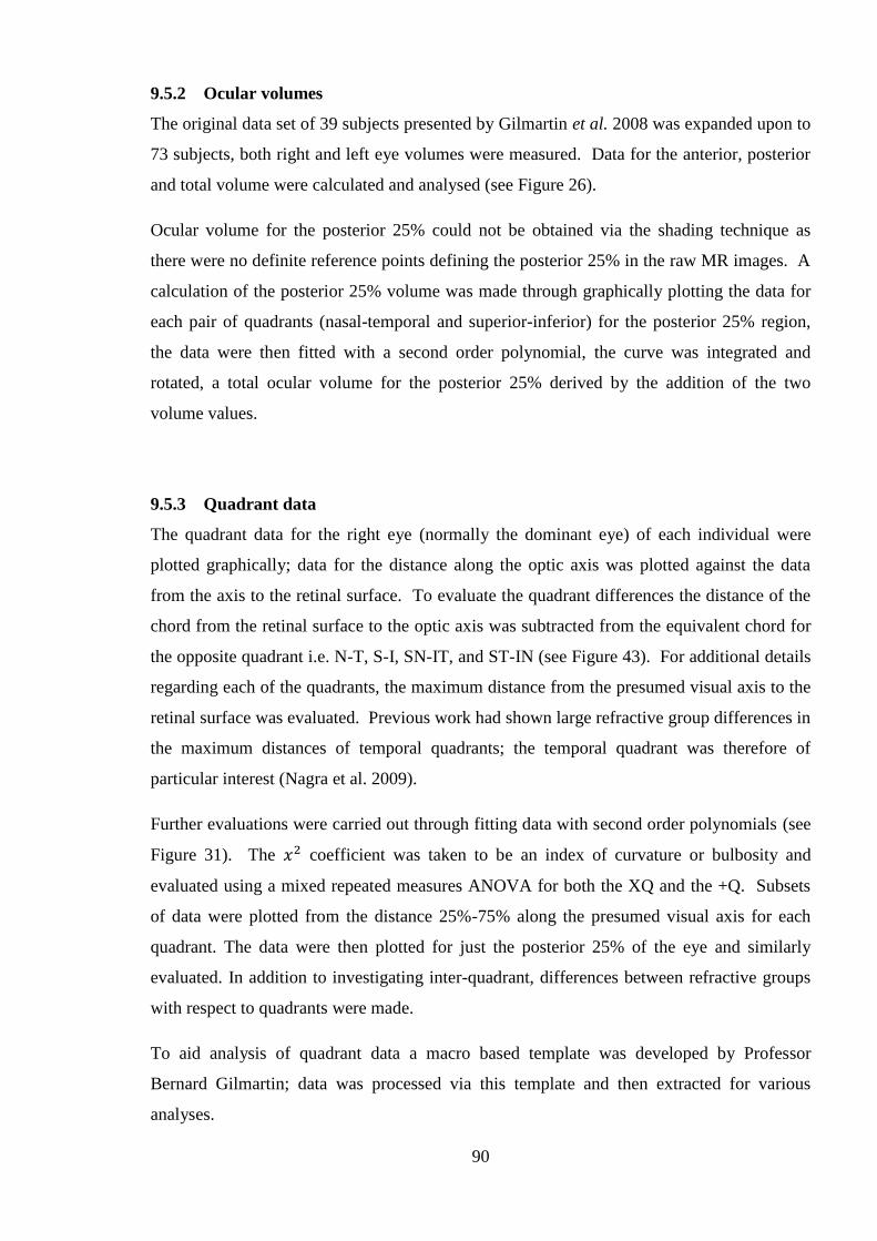
90

9.5.2 Ocular volumes

The original data set of 39 subjects presented by Gilmartin et al. 2008 was expanded upon to

73 subjects, both right and left eye volumes were measured. Data for the anterior, posterior

and total volume were calculated and analysed (see Figure 26).

Ocular volume for the posterior 25% could not be obtained via the shading technique as

there were no definite reference points defining the posterior 25% in the raw MR images. A

calculation of the posterior 25% volume was made through graphically plotting the data for

each pair of quadrants (nasal-temporal and superior-inferior) for the posterior 25% region,

the data were then fitted with a second order polynomial, the curve was integrated and

rotated, a total ocular volume for the posterior 25% derived by the addition of the two

volume values.

9.5.3 Quadrant data

The quadrant data for the right eye (normally the dominant eye) of each individual were

plotted graphically; data for the distance along the optic axis was plotted against the data

from the axis to the retinal surface. To evaluate the quadrant differences the distance of the

chord from the retinal surface to the optic axis was subtracted from the equivalent chord for

the opposite quadrant i.e. N-T, S-I, SN-IT, and ST-IN (see Figure 43). For additional details

regarding each of the quadrants, the maximum distance from the presumed visual axis to the

retinal surface was evaluated. Previous work had shown large refractive group differences in

the maximum distances of temporal quadrants; the temporal quadrant was therefore of

particular interest (Nagra et al. 2009).

Further evaluations were carried out through fitting data with second order polynomials (see

Figure 31). The coefficient was taken to be an index of curvature or bulbosity and

evaluated using a mixed repeated measures ANOVA for both the XQ and the +Q. Subsets

of data were plotted from the distance 25%-75% along the presumed visual axis for each

quadrant. The data were then plotted for just the posterior 25% of the eye and similarly

evaluated. In addition to investigating inter-quadrant, differences between refractive groups

with respect to quadrants were made.

To aid analysis of quadrant data a macro based template was developed by Professor

Bernard Gilmartin; data was processed via this template and then extracted for various

analyses.

91

Figure 31 Data plotted for the region 15-100% along the axis. 2nd

order polynomial fitted for

the region 25-75%.

9.5.4 Stretch index

To further examine the consequences of myopic growth, a stretch index was calculated as

the ratio of the width of the eye at a given point versus the axial length. This technique was

used for examining specific retinal locations; in this thesis the technique was used to

evaluate the point 40° temporal to the presumed foveal position (see 14.4).

9.5.5 Interval Variation (IV)

As a further measure of shape variation the standard deviations of the data comprising the

25-75% region of the eye and separately the posterior 25% of the eye, were derived and

interval variance calculated by multiplying standard deviations by a value of 1.96. Interval

variation was examined at every 5% increment along the axial length for the 25-75% region

and every 2.5% increment in the posterior 25%. The IVs were examined with reference to

refractive group and quadrants. The IV values helped evaluate the shape variance across

sections of the eye.

y = -0.0558x2 + 1.1468x + 6.6472

R² = 0.9917

0

2

4

6

8

10

12

14

16

3 5 7 9 11 13 15 17 19 21 23 25

Dis

tan

ce f

rom

axis

(m

m)

Distance along axis (mm)

92

9.5.6 Surface areas

The surface area for the posterior 25% of each quadrant was calculated through use of a

formula developed by Dr Brian Cox and Professor Bernard Gilmartin, (see chapters 12 and

13 for details).

9.5.7 Inter eye differences

A subset of 18 eyes were examined for inter eye differences; both XQ and +Q were

investigated. The data depicting the distance along the axis vs. distance to the retinal surface

were examined. Also comparisons between ocular volumes were made between right and

left eyes.

9.6 Results

9.6.1 Radius bands

The radius bands were plotted graphically; they detailed the equivalent radius of curvature in

1% increments along the geometric axis. For the region approximately 25% along the axis

to 75% along the axis, the low myopic and emmetropic groups showed a relatively constant

spherical shape. The radius data for the high myopes were flatter compared to other

refractive groups, but also maintained a spherical shape in this central region. The

hyperopes, although limited in number, showed steeper radius of curvature data compared to

other refractive groups in this central region (see Figure 32). A repeated measures ANOVA

evaluating the four quarters (0-25%, 25-50%, 50-75%, and 75-92%), showed no significant

differences between the 25-50 and 50-75% regions (p>0.05). There were significant

differences between the posterior 75-92% region and the 25-50 and 50-75% regions

(p>0.001). The only refractive group difference to reach significance was between

hyperopic group vs. emmetropic, low myopic, and also high myopic groups.

Posterior eye data were noisy due to eye movements and edge effect artefacts. Previous work

at Aston University involved a subject undergoing MR scanning 9 times; these data was used

to check repeatability using an ANOVA analysis (p>0.05) (Gilmartin et al. 2007).

Examination of the standard deviations for each of the refractive groups showed increased

values around the 92% point (the distance 92% along the axis); based on these previous

findings all data beyond the 92% region was omitted.

93

In the posterior region of the eye high myopes and low myopes showed relative steepening

of curvature; in contrast the emmetropic subjects showed relative flattening of curvature.

The hyperopic group comprised a limited number of subjects; results from the hyperopic

group showed relative flattening in the posterior region. Standard deviations were much

greater in the anterior 15% of the eye and fell sharply beyond this point. On average the

standard deviations in the anterior 15% for emmetropes, low myopes, high myopes and

hyperopes were ±2.92, 2.69, 2.96, and 3.65mm respectively. The standard deviations fell to

±0.61, 0.61, 0.86, and 0.87mm for the region beyond 15% along the axis.

Figure 32 The equivalent radius of curvature by refractive group. Each data set is fitted with a

moving average trendline; averaging every second point

8

9

10

11

12

13

14

15

16

17

0 10 20 30 40 50 60 70 80 90 100

RA

DIU

S O

F E

QU

IVA

LE

NT

SP

HE

RE

(m

m)

DISTANCE ALONG THE AXIS (%)

2 per. Mov. Avg. (EMMETROPES) 2 per. Mov. Avg. (LOW MYOPES)

2 per. Mov. Avg. (HIGH MYOPES) 2 per. Mov. Avg. (HYPEROPES)

94

Figure 33 Shows the standard deviation error bars for the emmetropic refractive group in the

region 15-92% along the axis

Figure 34 Shows the standard deviation error bars for the low myopic refractive group in the


8

9

10

11

12

13

14

15

16

10 20 30 40 50 60 70 80 90 100RA

DIU

S O

F E

QU

IVA

LE

NT

SP

HE

RE

(mm

)


EMMETROPES

8

9

10

11

12

13

14

15

16

10 20 30 40 50 60 70 80 90 100RA

DIU

S O

F E

QU

IVA

LE

NT

SP

HE

RE

(mm

)


LOW MYOPES

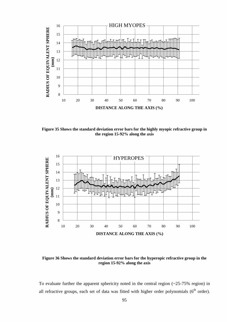
95

Figure 35 Shows the standard deviation error bars for the highly myopic refractive group in

the region 15-92% along the axis

Figure 36 Shows the standard deviation error bars for the hyperopic refractive group in the


To evaluate further the apparent sphericity noted in the central region (~25-75% region) in

all refractive groups, each set of data was fitted with higher order polynomials (6th

order).

8

9

10

11

12

13

14

15

16

10 20 30 40 50 60 70 80 90 100

RA

DIU

S O

F E

QU

IVA

LE

NT

SP

HE

RE

(mm

)


HIGH MYOPES

8

9

10

11

12

13

14

15

16

10 20 30 40 50 60 70 80 90 100RA

DIU

S O

F E

QU

IVA

LE

NT

SP

HE

RE

(mm

)


HYPEROPES

96

Although each refractive group showed a region of sphericity for some part of the central

region, variations were evident following through fitting of higher order polynomial curves.

The region of sphericity began at a distance approximately 40% along the axis, unlike the

previously proposed 25% mark (see 9.6.1). The total region of sphericity was largest for the

high myopes and hyperopes. The emmetropes and low myopes showed the greatest amount

of variation.

Figure 37 The equivalent radius data fitted with 6th

order polynomials to expose subtle changes

in shape

9.6.2 Ocular volumes

Anterior vs. Posterior volumes

Ocular volumes were calculated using the same methodology as previously reported by

Gilmartin et al. 2008. Ocular volume for the posterior 25% could not be obtained via the

11.5

11.7

11.9

12.1

12.3

12.5

12.7

12.9

13.1

13.3

13.5

13.7

13.9

20 25 30 35 40 45 50 55 60 65 70 75 80

RA

DIU

S O

F E

QU

IVA

LE

NT

SP

HE

RE

(m

m)


Poly. (EMMETROPES) Poly. (LOW MYOPES)

Poly. (HIGH MYOPES) Poly. (HYPEROPES)

97

shading technique due to limitations in determining the reference points defining the

posterior 25%; therefore a calculation through integration was used to derive volume in this

region.

Subject data for the posterior and anterior volumes was plotted as a function of refractive

error. The results supported earlier findings which showed the anterior volume was constant

across all refractive groups, and posterior volume increased linearly as a function of

increasing myopia. Gilmartin et al. (2008) reported R² values for posterior volume vs. MSE

of 0.53 and 0.01 for anterior volume vs. MSE. The current study showed similar values (see

Figure 38). A Pearson‘s one tailed correlation coefficient showed the posterior volume

correlation with MSE to be significant (p=<0.01, r = -0.676), and as expected there was no

significant relationship between anterior volumes and MSE (p>0.05, r = 0.121) or between

anterior volume and posterior volume (p>0.05). The overall total volume was significantly

correlated with MSE (p=<0.01).

Figure 38 The anterior volumes (below in grey) and posterior volumes (above in black) plotted

as a function of MSE. Data is shown for RE only (n=73).

y = -196.77x + 6557.7

R² = 0.457

y = 4.367x + 1112

R² = 0.0146

0

2000

4000

6000

8000

10000

12000

-12 -10 -8 -6 -4 -2 0 2 4 6

Ocu

lar

volu

me (

in m

m³)

MSE (in D)

POSTERIOR VOLUME ANTERIOR VOLUME

98

Posterior 25% cap volume (calculated through integration of polynomial curves)

The posterior 25% volumes showed an increase in volume which corresponded with an

increase in myopia.

Figure 39 The volume for the posterior 25% plotted as a function of MSE

The volume for the posterior 25% cap of the eye was then subtracted from the posterior

volume defined earlier as the region between the retinal surface and the posterior crystalline

lens. The results showed that the posterior 25% volume made little difference to the

posterior volume vs. MSE relationship (see Figure 40).

y = -23.782x + 1183

R² = 0.2773

0

200

400

600

800

1000

1200

1400

1600

1800

2000

-15 -10 -5 0 5 10 15

Vo

lum

e (

in m

m³)

MSE (in D)

99

Figure 40 The posterior volume minus the posterior 25% volume

In order to investigate the ocular volume further, corneal volumes were measured using the

Oculus Pentacam on a subset of 42 subjects, mean MSE -2.05±3.69D (see Figure 41).

Corneal volume did not show a significant correlation with MSE, which reaffirms the notion

that the volume of the anterior eye is not affected by ocular shape changes present in

myopia.

y = -174.82x + 5367.7

R² = 0.5011

0

1000

2000

3000

4000

5000

6000

7000

8000

9000

10000

-14 -9 -4 1 6 11

Vo

lum

e (

in m

m³)

MSE (in D)

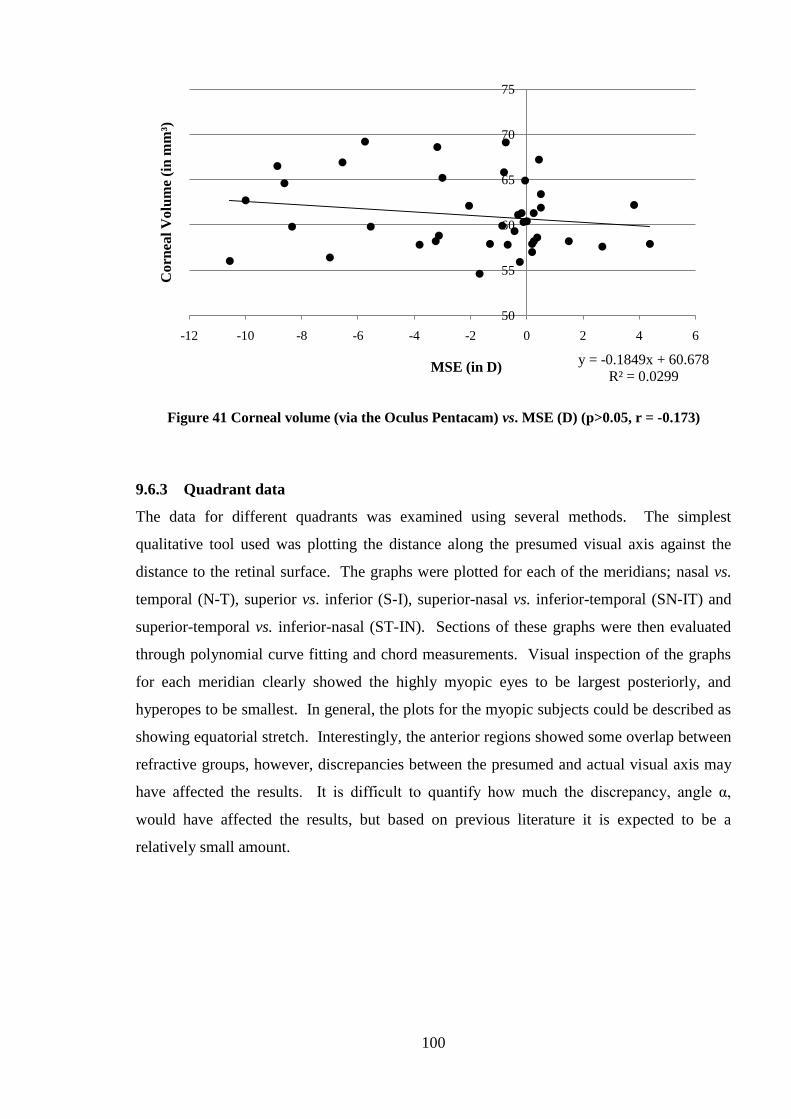
100

Figure 41 Corneal volume (via the Oculus Pentacam) vs. MSE (D) (p>0.05, r = -0.173)

9.6.3 Quadrant data

The data for different quadrants was examined using several methods. The simplest

qualitative tool used was plotting the distance along the presumed visual axis against the

distance to the retinal surface. The graphs were plotted for each of the meridians; nasal vs.

temporal (N-T), superior vs. inferior (S-I), superior-nasal vs. inferior-temporal (SN-IT) and

superior-temporal vs. inferior-nasal (ST-IN). Sections of these graphs were then evaluated

through polynomial curve fitting and chord measurements. Visual inspection of the graphs

for each meridian clearly showed the highly myopic eyes to be largest posteriorly, and

hyperopes to be smallest. In general, the plots for the myopic subjects could be described as

showing equatorial stretch. Interestingly, the anterior regions showed some overlap between

refractive groups, however, discrepancies between the presumed and actual visual axis may

have affected the results. It is difficult to quantify how much the discrepancy, angle α,

would have affected the results, but based on previous literature it is expected to be a

relatively small amount.

y = -0.1849x + 60.678

R² = 0.0299

50

55

60

65

70

75

-12 -10 -8 -6 -4 -2 0 2 4 6

Co

rnea

l V

olu

me (

in m

m³)

MSE (in D)

101

-20

-15

-10

-5

0

5

10

15

20

0 5 10 15 20 25 30

Dis

tan

ce f

rom

th

e a

xis

(m

m)

Distance along the presumed visual axis (mm)

High Myopes

Low Myopes

Emmetropes

Hyperopes

N

T

-20

-15

-10

-5

0

5

10

15

20

0 5 10 15 20 25 30

Dis

tan

ce f

rom

th

e axis

(m

m)


High Myopes

Low Myopes

Emmetropes

Hyperopes

S

I

102

Figure 42 A graphical representation of the retinal contours by quadrant

-20

-15

-10

-5

0

5

10

15

20

0 5 10 15 20 25 30

Dis

tan

ce f

rom

th

e a

xis

(m

m)


High Myopes

Low Myopes

Emmetropes

Hyperopes

ST

IN

-20

-15

-10

-5

0

5

10

15

20

0 5 10 15 20 25 30

Dis

tan

ce f

rom

th

e axis

(m

m)


High Myopes

Low Myopes

Emmetropes

Hyperopes

SN

IT

103

Chord differences

To evaluate quadrant differences, the chord distances between two parallel quadrants or

meridians i.e. N-T, S-I, SN-IT, and ST-IN, were calculated and plotted graphically (see

Figure 43).

Figure 43 Nasal and temporal chord distances. Temporal chord distances were subtracted from

nasal and plotted graphically. The same methodology was used for S-I, SN-IT and ST-IN

quadrants.

Quadrants: XQ

The N-T chord differences appeared to follow the same basic pattern for all refractive groups

for the region ~15-75% along the optic axis. Interestingly the N-T chord differences in the

posterior region appeared to be at similar levels for all refractive groups at approximately

75% along the axis, the difference values between nasal and temporal chords at this cross

over point ranged from approximately 0.1-0.05mm. In general the nasal chord was larger

than that of the temporal up to the ~75% mark; beyond this point the hyperopes and

emmetropes showed the temporal chord to be larger than the nasal (hence the negative

values when the temporal chord value is subtracted from the nasal). A repeated measures

ANOVA was carried out to compare chord differences up to the 76.25% mark and then

beyond the 76.25% mark; 76.25% was selected as it was the closest point to 75% for which

values had been derived. For chord differences up to the 76.25% mark results showed

significant differences between all refractive groups (p<0.001). Chord differences beyond

the 76.25% mark showed significant refractive group differences between all groups

(p<0.05) bar the high myopes vs. low myopes, low myopes vs. emmetropes, and emmetropes

vs. hyperopes.

104

Figure 44 Differences between the nasal and temporal chords in each refractive group

A repeated measures ANOVA for superior-inferior chord differences up to the 76.25% mark

showed significant refractive group differences between all groups (p<0.05) bar the low

myopic vs. hyperopic group. In the posterior region significant refractive group differences

were noted for all groups (p<0.05) bar the high myopic vs. low myopic and high myopic vs.

emmetropic groups.

-0.5

0.0

0.5

1.0

1.5

2.0

2.5

15.0 35.0 55.0 75.0 95.0Dif

fere

nce

bet

wee

n N

asa

l a

nd

Tem

po

ral

cho

rds

(mm

)

Distance along the axis (%)

Nasal-Temporal chord differences

High Myopes Low Myopes Emmetropes Hyperopes

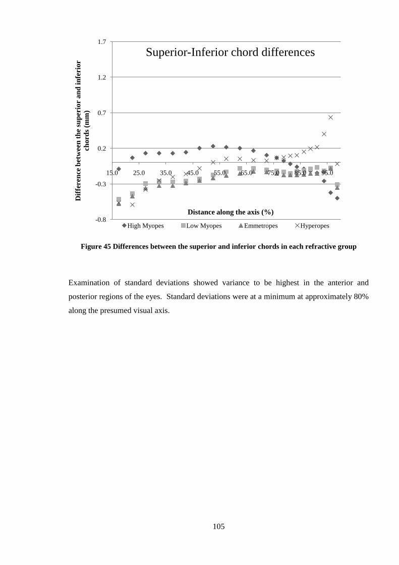
105

Figure 45 Differences between the superior and inferior chords in each refractive group

Examination of standard deviations showed variance to be highest in the anterior and

posterior regions of the eyes. Standard deviations were at a minimum at approximately 80%

along the presumed visual axis.

-0.8

-0.3

0.2

0.7

1.2

1.7

15.0 25.0 35.0 45.0 55.0 65.0 75.0 85.0 95.0

Dif

fere

nce

bet

wee

n t

he

sup

erio

r a

nd

in

feri

or

cho

rds

(mm

)


Superior-Inferior chord differences


106

Figure 46 Standard deviations for each refractive group, nasal-temporal quadrants

Figure 47 Standard deviations for each refractive group, superior-inferior quadrants

0.000

0.200

0.400

0.600

0.800

1.000

1.200

1.400

0.0 20.0 40.0 60.0 80.0 100.0

Sta

nd

ard

dev

iati

on

fo

r n

asa

l-te

mp

ora

l ch

ord

dif

fere

nce

s (i

n m

m)

Distance along presumed visual axis (%)

High Myopes

Low Myopes

Emmetropes

Hyperopes

0.000

0.200

0.400

0.600

0.800

1.000

1.200

1.400

0.0 20.0 40.0 60.0 80.0 100.0

Sta

nd

ard

dev

iati

on

for

sup

erio

r-i

nfe

rior

chord

dif

fere

nce

s (i

n m

m)

Distance along the presumed visual axis (%)

High Myopes

Low Myopes

Emmetropes

Hyperopes

107

Quadrants: +Q

A repeated measures ANOVA for the region 17.5-76.25% showed significant refractive

group differences between all groups (p<0.05), bar the high myopic vs. low myopic and

highly myopic vs. hyperopic groups. Results for the region posterior to the 76.25% mark

showed significant refractive group differences for the hyperopic vs. emmetropic, high

myopic and low myopic refractive groups. Significant refractive group differences in this

region were also noted between the low myopic and emmetropic groups

In general the SN chord appeared to be larger than the IT; however in the posterior region of

the eye the SN chord was noticeably smaller than the IT for the hyperopic group.

Figure 48 The differences between the SN and IT chords for each refractive group

-0.8

-0.3

0.2

0.7

1.2

1.7

15.0 35.0 55.0 75.0 95.0

Dis

tan

ce b

etw

een

th

e S

N-I

T c

hord

s (i

n m

m)


SN-IT chord differences


108

Figure 49 The differences between the ST and IN chords for each refractive group. NB scaling

differences of y axis compared to SN-IT chord differences graph

The ST-IN chords showed the IN to be larger than the ST, but again changes were noted

beyond ~75% (see Figure 49). For the region 17.5-76.25% along the presumed visual axis, a

significant refractive group difference was noted for all groups (p<0.01). Beyond the

76.25% mark, refractive group differences failed to reach significance (p>0.05)

The standard deviations were plotted for both ST-IN and SN-IT chord differences. Unlike

the XQ, the standard deviations for the chord differences did not appear to follow a strict

pattern, however for each refractive group at around 80-85% along the presumed axis the

standard deviations for chord differences appeared to be at their lowest.

-2.0

-1.5

-1.0

-0.5

0.0

0.5

1.0

1.5

15.0 35.0 55.0 75.0 95.0

Dif

fere

nce

bet

wee

n t

he

ST

-IN

ch

ord

s

(mm

)


ST-IN chord differences


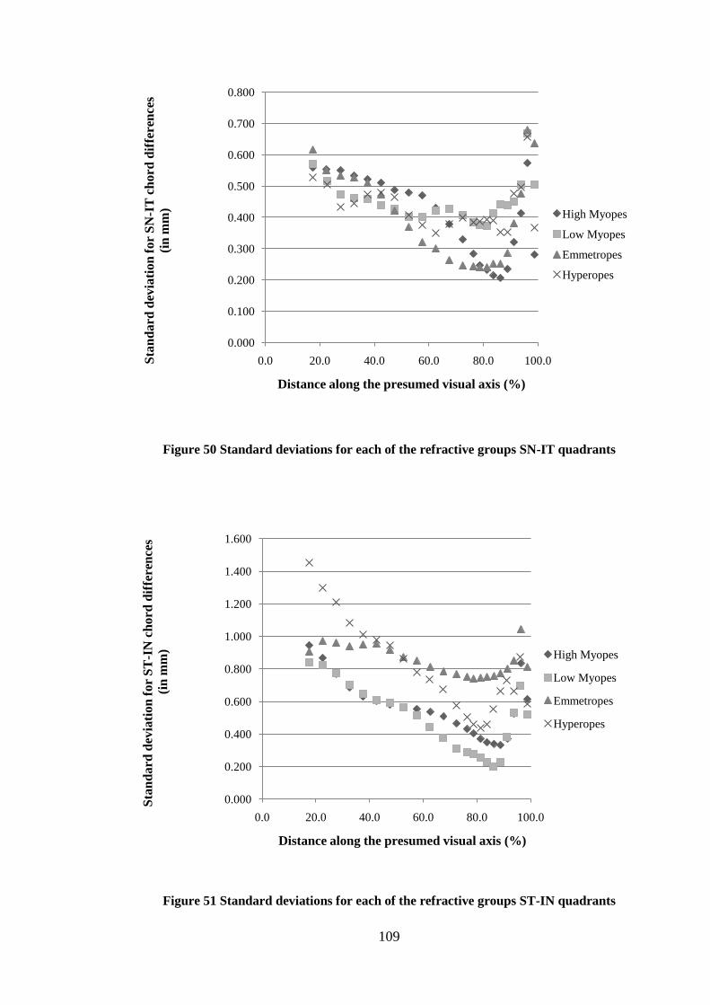
109

Figure 50 Standard deviations for each of the refractive groups SN-IT quadrants

Figure 51 Standard deviations for each of the refractive groups ST-IN quadrants

0.000

0.100

0.200

0.300

0.400

0.500

0.600

0.700

0.800

0.0 20.0 40.0 60.0 80.0 100.0Sta

nd

ard

dev

iati

on

fo

r S

N-I

T c

ho

rd d

iffe

ren

ces

(in

mm

)


High Myopes

Low Myopes

Emmetropes

Hyperopes

0.000

0.200

0.400

0.600

0.800

1.000

1.200

1.400

1.600

0.0 20.0 40.0 60.0 80.0 100.0

Sta

nd

ard

dev

iati

on

for

ST

-IN

ch

ord

dif

fere

nce

s

(in

mm

)


High Myopes

Low Myopes

Emmetropes

Hyperopes

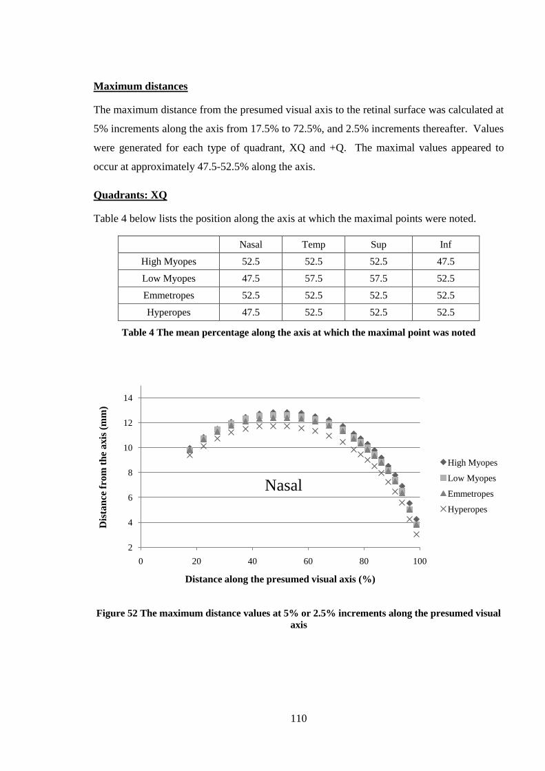
110

Maximum distances

The maximum distance from the presumed visual axis to the retinal surface was calculated at

5% increments along the axis from 17.5% to 72.5%, and 2.5% increments thereafter. Values

were generated for each type of quadrant, XQ and +Q. The maximal values appeared to

occur at approximately 47.5-52.5% along the axis.

Quadrants: XQ

Table 4 below lists the position along the axis at which the maximal points were noted.

Nasal Temp Sup Inf

High Myopes 52.5 52.5 52.5 47.5

Low Myopes 47.5 57.5 57.5 52.5

Emmetropes 52.5 52.5 52.5 52.5

Hyperopes 47.5 52.5 52.5 52.5

Table 4 The mean percentage along the axis at which the maximal point was noted

Figure 52 The maximum distance values at 5% or 2.5% increments along the presumed visual

axis

2

4

6

8

10

12

14

0 20 40 60 80 100

Dis

tan

ce f

rom

th

e axis

(m

m)


Nasal

High Myopes

Low Myopes

Emmetropes

Hyperopes

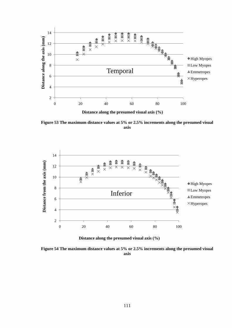
111


axis


axis

2

4

6

8

10

12

14

0 20 40 60 80 100

Dis

tan

ce a

lon

g t

he

axis

(m

m)


Temporal

High Myopes

Low Myopes

Emmetropes

Hyperopes

2

4

6

8

10

12

14

0 20 40 60 80 100

Dis

tan

ce f

rom

th

e a

xis

(m

m)


Inferior

High Myopes

Low Myopes

Emmetropes

Hyperopes

112


axis


quadrant

2

4

6

8

10

12

14

0 20 40 60 80 100

Dis

tan

ce f

rom

th

e axii

s (m

m)


Superior

High Myopes

Low Myopes

Emmetropes

Hyperopes

11

11.5

12

12.5

13

13.5

14

14.5

NASAL TEMP SUP INF

Dis

tan

ce f

rom

vis

ual

axis

(m

m)

Quadrant

High Myopes

Low Myopes

Emmetropes

Hyperopes

113

A repeated measures ANOVA showed a significant refractive group, and separately, a

significant quadrant effect was noted (p<0.01). The maximum distances were largest in the

highly myopic subjects and declined as a function of decreasing myopia. The largest

maximal distance was noted in the superior quadrant for each refractive group. The smallest

maximum distance was noted in the nasal quadrant, this was also the same for each

refractive group. All quadrant differences were significant (p<0.05) bar the nasal vs. inferior

comparison (p>0.05). Refractive group differences were significant between the hyperopic

group vs. all other refractive groups (p<0.05).

To further describe the differences between refractive groups the mean maximal values

between individual quadrants were examined. Of particular interest were the differences

between high myopes vs. other refractive groups. In line with the previous experiment, the

maximum distances of the highly myopic group exceeded other refractive groups for all

quadrants; the differences were particularly marked for the temporal quadrant. Comparisons

of the mean maximum distances for high myopes with other refractive groups revealed that

on average the increases in ascending order were: superior = 0.58±0.47mm, inferior =

0.58±0.46mm, nasal = 0.60±0.45mm, and temporal = 0.77±0.46mm. The results mirror

those of an earlier study conducted using the same techniques where emmetropic and

myopic subjects were compared (Nagra et al. 2009). A difference in temporal quadrant

maximum distances was also noted in comparisons between the low myopic vs. emmetropic

group, and between low myopic and hyperopic groups. One anomaly to this pattern was the

emmetropic vs. hyperopic comparison.

Nasal max

±sd

(mm) Temp max

±sd

(mm) Sup max

±sd

(mm) Inf max

±sd

(mm)

High Myopes 12.85 ±0.71 13.86 ±0.68 13.88 ±0.68 12.95 ±0.63

Low Myopes 12.59 ±0.67 13.44 ±0.64 13.59 ±0.55 12.67 ±0.43

Emmetropes 12.41 ±0.54 13.26 ±0.54 13.56 ±0.46 12.60 ±0.46

Hyperopes 11.74 ±0.77 12.56 ±0.88 12.76 ±0.75 11.84 ±0.56

Table 5 Mean maximum distance for each quadrant by refractive group. SD indicates the

standard deviation of the maximum distance values for each refractive group

114

Quadrants: +Q

The results showed a significant refractive group effect, and separately, a significant

quadrant effect (p<0.05). All quadrants showed significant differences (p<0.05) except the

ST vs. IT comparison. Refractive group differences were significant for all refractive group

vs. the hyperopic group, and the highly myopic vs. emmetropic groups (p<0.05).

The table below shows the position at which maximal distances were noted for each of the

quadrants by refractive group.

ST IN SN IT

High Myopes 52.5 52.5 52.5 52.5

Low Myopes 52.5 47.5 52.5 52.5

Emmetropes 52.5 47.5 52.5 52.5

Hyperopes 52.5 47.5 52.5 52.5

Table 6 Lists the distance in mean percentage along the axis at which the maximal point was

noted

115

Figure 57 Maximum distance values at 5% or 2.5% increments along the presumed visual axis


0

2

4

6

8

10

12

14

16

0 20 40 60 80 100

Dis

tan

ce f

rom

th

e a

xis

(m

m)


Sup-Temp

High Myopes

Low Myopes

Emmetropes

Hyperopes

0

2

4

6

8

10

12

14

0 20 40 60 80 100

Dis

tan

ce f

rom

th

e axis

(m

m)


Inf-Nasal

High Myopes

Low Myopes

Emmetropes

Hyperopes

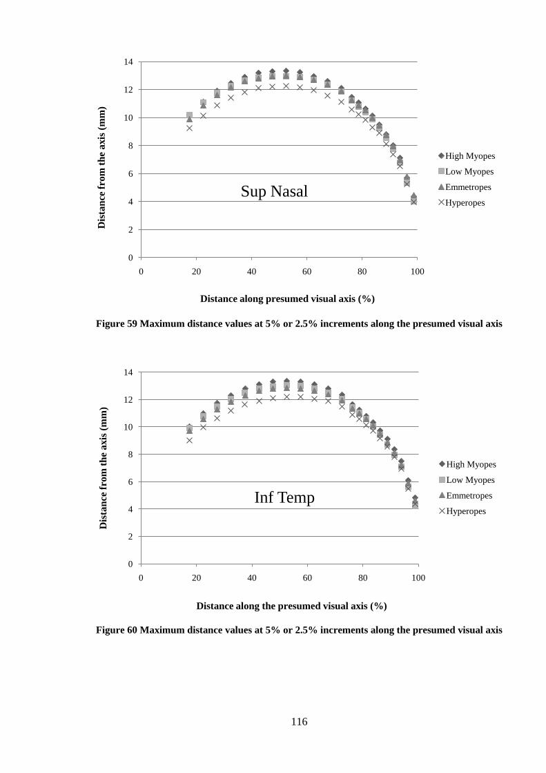
116



0

2

4

6

8

10

12

14

0 20 40 60 80 100

Dis

tan

ce f

rom

th

e a

xis

(m

m)


Sup Nasal

High Myopes

Low Myopes

Emmetropes

Hyperopes

0

2

4

6

8

10

12

14

0 20 40 60 80 100

Dis

tan

ce f

rom

th

e axis

(m

m)


Inf Temp

High Myopes

Low Myopes

Emmetropes

Hyperopes

117


quadrant

All refractive groups showed the maximum values in the ST quadrant to be largest and IN to

be the smallest (see Figure 61). Comparisons of maximum distance between high myopes

and other refractive groups showed the largest differences in the ST quadrants. Using

average maximum distance values the ST quadrant was larger in high myopes compared

with other refractive groups by 0.68±0.45mm; in comparison the IT quadrant was larger by

0.64±0.44mm, IN by 0.58±0.45mm, and SN by 0.58±0.45mm. Maximum distance in low

myopes minus maximum distance in hyperopes also showed the ST quadrant differences to

be largest. In contrast, other refractive group combinations (i.e. low myopes minus

emmetropes, emmetropes minus hyperopes) did not show any clear pattern.

ST max

±sd

(mm) IN max

±sd

(mm) SN max

±sd

(mm) IT max

±sd

(mm)

High Myopes 14.06 ±0.64 12.73 ±0.66 13.32 ±0.65 13.34 ±0.64

Low Myopes 13.71 ±0.55 12.45 ±0.54 12.96 ±0.33 13.03 ±0.52

Emmetropes 13.56 ±0.42 12.36 ±0.38 13.00 ±0.44 12.86 ±0.41

Hyperopes 12.87 ±0.77 11.63 ±0.54 12.24 ±0.75 12.19 ±0.96

Table 7 Showing the maximum distance for each quadrant by refractive group. SD indicates

the standard deviation

11.0

11.5

12.0

12.5

13.0

13.5

14.0

14.5

ST IN SN IT

Dis

tan

ce f

rom

vis

ua

l a

xis

(m

m)

Quadrant

High Myopes

Low Myopes

Emmetropes

Hyperopes

118

Polynomial equations

Data for each quadrant was plotted for the region 25-75% along the presumed visual axis;

data were fitted with second order polynomials using Microsoft Excel and the coefficient

of the polynomial equation analysed in order to assess bulbosity.

Quadrants: XQ

The coefficients for each of the quadrants were examined with reference to refractive

group. A 2-way mixed repeated measures ANOVA showed that although the between-

subject effects of refractive error were significant (p<0.01) and the differences in quadrants

within subjects were also significant (p<0.01), the quadrant: refractive group interaction was

not significant (p>0.05). The significant refractive group differences were principally

differences between the hyperopic group and other refractive groups (p<0.01). Within-

subject quadrant effects showed all interactions bar the nasal vs. superior (0.229) and inferior

vs. temporal (p = 0.279) to be significant (p<0.01).

Visual inspection of the graphs showed that in general the inferior quadrant appeared to be

most bulbous; however in hyperopic subjects the superior quadrant was most bulbous. The

least bulbous quadrant varied depending on refractive group; the emmetropes and low

myopes showed the least bulbous quadrant to be the nasal quadrant; the high myopes and

hyperopes showed the least bulbous quadrant to be the temporal quadrant.

119

Figure 62 The mean x² coefficient values for each quadrant divided further by refractive group

The coefficient corresponding to data comprising the posterior 25% cap of the eye was

examined for the N-T meridian and the S-I meridian. Visual inspection of the data showed

the N-T meridian to be more bulbous than the I-N for all refractive groups, bar the high

myopes.

Figure 63 The mean x² coefficient values for the polynomial curves fitted to data representing

the posterior 25% cap of the eye. Data are separated by refractive group

-0.08 -0.07 -0.06 -0.05 -0.04 -0.03 -0.02 -0.01 0.00

X² NASAL 25-75

X² TEMP 25-75

X² SUP 25-75

X² INF 25-75

X² value

Qu

ad

ran

t

Hyperopes Emmetropes Low Myopes High Myopes

-0.06 -0.05 -0.04 -0.03 -0.02 -0.01 0

High Myopes

Low Myopes

Emmetropes

Hyperopes

x^2 coefficient for the posterior 25% polynomial

S:I N:T

120

A repeated measures ANOVA showed the meridian differences were not significant

(p=0.072). Furthermore the meridian: refractive group difference was also not significant

(p=0.457). A significant between-subjects refractive error effect was noted (p =0.011); post

hoc tests revealed the refractive group differences to lie between the high myopes and

emmetropes (p = <0.01).

Quadrants: +Q

The coefficient for +Q was then examined using the same methodology described above.

Unlike the XQ, a 2-way mixed repeated measures ANOVA showed the between subjects

effect of refractive error was not significant.

Similar to the XQ the quadrant: refractive group interaction was not significant whilst the

within subjects quadrant effect was significant (p<0.01).

Quadrant pairwise interaction were significant for all combinations except the ST vs. SN and

IN vs. IT. The results for the 25-75% along the axis region showed the least bulbous

quadrant to be the IN; this was the case for all refractive groups. There was no clear pattern

regarding which was the most bulbous quadrant.

Figure 64 The mean x² coefficient values for each quadrant divided further by refractive group

-0.07 -0.06 -0.05 -0.04 -0.03 -0.02 -0.01 0.00

X² SUP TEMP 25-75

X² INF NASAL 25-75

X² SUPNASAL 25-75

X² INF TEMP 25-75

X² value

Qu

ad

ran

t


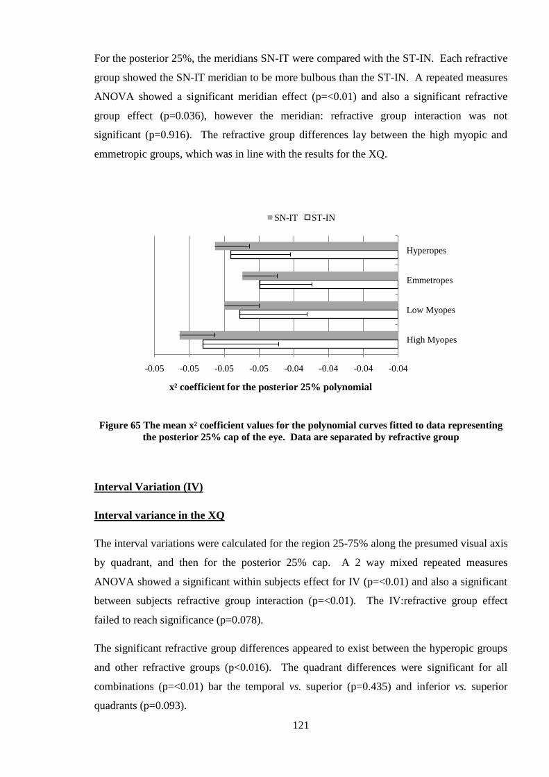
121

For the posterior 25%, the meridians SN-IT were compared with the ST-IN. Each refractive

group showed the SN-IT meridian to be more bulbous than the ST-IN. A repeated measures

ANOVA showed a significant meridian effect (p=<0.01) and also a significant refractive

group effect (p=0.036), however the meridian: refractive group interaction was not

significant (p=0.916). The refractive group differences lay between the high myopic and

emmetropic groups, which was in line with the results for the XQ.

Figure 65 The mean x² coefficient values for the polynomial curves fitted to data representing

the posterior 25% cap of the eye. Data are separated by refractive group

Interval Variation (IV)

Interval variance in the XQ

The interval variations were calculated for the region 25-75% along the presumed visual axis

by quadrant, and then for the posterior 25% cap. A 2 way mixed repeated measures

ANOVA showed a significant within subjects effect for IV (p=<0.01) and also a significant

between subjects refractive group interaction (p=<0.01). The IV:refractive group effect

failed to reach significance (p=0.078).

The significant refractive group differences appeared to exist between the hyperopic groups

and other refractive groups (p<0.016). The quadrant differences were significant for all

combinations (p=<0.01) bar the temporal vs. superior (p=0.435) and inferior vs. superior

quadrants (p=0.093).

-0.05 -0.05 -0.05 -0.05 -0.04 -0.04 -0.04 -0.04

High Myopes

Low Myopes

Emmetropes

Hyperopes

x² coefficient for the posterior 25% polynomial

SN-IT ST-IN

122

The results showed the IV for the nasal quadrant was smallest in all refractive groups; the

largest quadrant was the temporal in all subjects bar the high myopes who showed the

superior quadrant to be marginally greater than the temporal (by 0.01mm).

Figure 66 The mean Interval Variance (IV) shown for the XQ

Results for the posterior 25% were calculated in the N-T meridian and the S-I meridian. A

repeated measures ANOVA showed the meridian effect to be significant (p=0.021). The

meridian: refractive group interaction and between subjects refractive group effects were not

significant (p=<0.01). Overall the results indicated that although there were significant

quadrant differences they were largely unaffected by refractive group.

0 0.5 1 1.5 2 2.5 3 3.5

IV NASAL 25-75

IV TEMP 25-75

IV SUP 25-75

IV INF 25-75

Interval Variance (IV) in mm

Qu

ad

ran

t


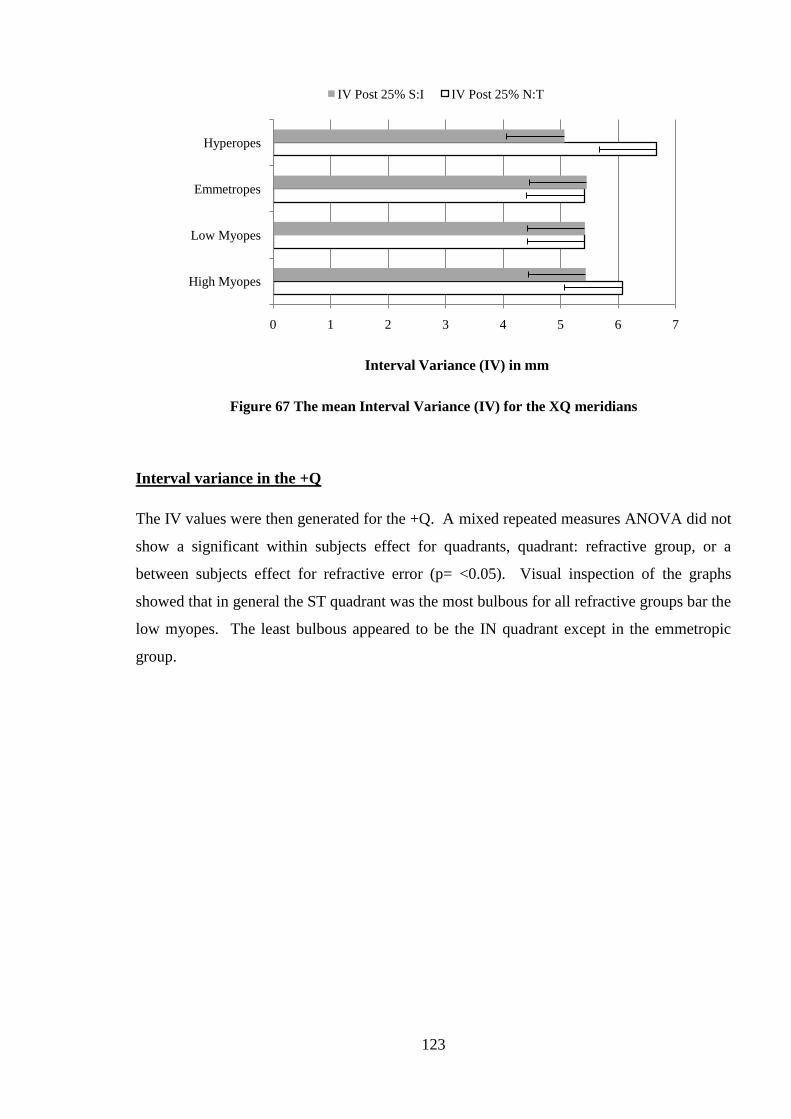
123

Figure 67 The mean Interval Variance (IV) for the XQ meridians

Interval variance in the +Q

The IV values were then generated for the +Q. A mixed repeated measures ANOVA did not

show a significant within subjects effect for quadrants, quadrant: refractive group, or a

between subjects effect for refractive error (p= <0.05). Visual inspection of the graphs

showed that in general the ST quadrant was the most bulbous for all refractive groups bar the

low myopes. The least bulbous appeared to be the IN quadrant except in the emmetropic

group.

0 1 2 3 4 5 6 7

High Myopes

Low Myopes

Emmetropes

Hyperopes


IV Post 25% S:I IV Post 25% N:T

124

Figure 68 The mean Interval Variance (IV) for the +Q in the 25-75% region

The meridians SN-IT and ST-IN in the posterior 25% did not show significant differences

for meridian or refractive group effects (p= >0.05). Similarly, the meridian: refractive group

interaction was not significant (p=0.923).

Overall, unlike the XQ, the +Q showed little difference between quadrants; refractive group

differences were not noted either.

-0.25 0.25 0.75 1.25 1.75 2.25

IV ST 25-75

IV IN 25-75

IV SN 25-75

IV IT 25-75


Qu

ad

ran

t


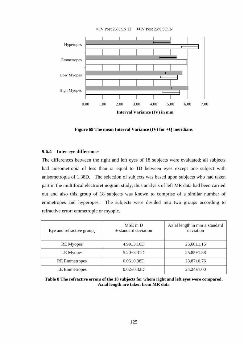
125

Figure 69 The mean Interval Variance (IV) for +Q meridians

9.6.4 Inter eye differences

The differences between the right and left eyes of 18 subjects were evaluated; all subjects

had anisometropia of less than or equal to 1D between eyes except one subject with

anisometropia of 1.38D. The selection of subjects was based upon subjects who had taken

part in the multifocal electroretinogram study, thus analysis of left MR data had been carried

out and also this group of 18 subjects was known to comprise of a similar number of

emmetropes and hyperopes. The subjects were divided into two groups according to

refractive error: emmetropic or myopic.

Eye and refractive group¸

MSE in D

± standard deviation

Axial length in mm ± standard

deviation

RE Myopes 4.99±3.16D

25.60±1.15

LE Myopes 5.20±3.31D

25.85±1.38

RE Emmetropes 0.06±0.38D

23.87±0.76

LE Emmetropes 0.02±0.32D

24.24±1.00

Table 8 The refractive errors of the 18 subjects for whom right and left eyes were compared.

Axial length are taken from MR data

0.00 1.00 2.00 3.00 4.00 5.00 6.00 7.00

High Myopes

Low Myopes

Emmetropes

Hyperopes


IV Post 25% SN:IT IV Post 25% ST:IN

126

Quadrants: XQ

The inter eye differences in distance to the retinal surface from the presumed visual axis

were calculated for both emmetropic and myopic eyes by quadrant. The differences in

values were plotted against the distance along the presumed visual axis. Results for the nasal

and temporal quadrants showed that the right and left eyes differed most in the anterior

region of the eye. The superior and inferior quadrants showed dissimilar patterns of inter

eye differences between the refractive groups unlike the nasal and temporal quadrants where

patterns were largely similar between both quadrants and refractive groups. In general, nasal

and temporal inter eye differences were larger than the superior and inferior. In order to

reduce the effects of angle alpha, statistical analysis was carried out for the N-T and S-I

meridians rather than individual quadrants. Both the emmetropic and myopic refractive

groups showed significant inter eye differences for the N-T meridians (p<0.01). For the

superior-inferior regions only myopic eyes showed significant inter eye differences (p<0.01).

The graphs which follow show differences of left eyes values minus right eyes values.

Figure 70 The mean differences between the right and left eyes of emmetropic and myopic

refractive groups for the nasal and temporal quadrants.

-1.60

-1.40

-1.20

-1.00

-0.80

-0.60

-0.40

-0.20

0.00

0.20

0.40

10 20 30 40 50 60 70 80 90 100

Dif

fere

nce

bet

wee

n r

igh

t an

d l

eft

eye

qu

ad

ran

ts (

mm

)


Myopic Nasal Myopic Temporal Emmetropic Nasal Emmetropic Temporal

127


refractive groups for the superior and inferior quadrants

Figure 72 Standard deviations (SD) for the nasal and temporal inter eye differences

-0.6

-0.4

-0.2

0

0.2

0.4

0.6

10 20 30 40 50 60 70 80 90 100

Dif

fere

nce

bet

wee

n r

igh

t a

nd

lef

t ey

e

qu

ad

ran

ts (

mm

)

Distance along axis (%)

Myopic Superior Myopic Inferior Emmetropic Superior Emmetropic Inferior

0.00

0.20

0.40

0.60

0.80

1.00

1.20

1.40

10 20 30 40 50 60 70 80 90 100

Sta

nd

ard

dev

iati

on

s of

inte

r ey

e d

iffe

ren

ces

sho

win

g d

ista

nce

fro

m t

he

axis

(m

m)


Myopic Nasal SD Myopic Temporal SD Emmetropic Nasal SD Emmetropic Temporal SD

128

Figure 73 Standard deviations (SD) for the superior and inferior inter eye differences

Quadrants: +Q

Statistical analysis showed significant inter eye differences for both the myopic and

emmetropic groups (p<0.01) for the SN-IT and ST-IN meridians. Visual inspection of the

graphs showed differences between the right and left eyes to be generally larger in the more

anterior aspects of the eye, but gradually decreasing up to the mid section of the eye

(approximately 50-70% along the axis), before gradually increasing again.

0.00

0.20

0.40

0.60

0.80

1.00

1.20

1.40

1.60

10 20 30 40 50 60 70 80 90 100

Sta

nd

ard

dev

iati

on

s o

f in

ter

eye

dif

fere

nce

s sh

ow

ing

dis

tan

ce f

rom

th

e a

xis

(m

m)


Myopic Superior SD Myopic Inferior SD Emmetropic Superior SD Emmetropic Inferior SD

129


refractive groups for the SN and IT quadrants


refractive groups for the ST and IN quadrants

-0.5

-0.4

-0.3

-0.2

-0.1

0

0.1

0.2

0.3

0.4

0.5

10 20 30 40 50 60 70 80 90 100

Dis

tan

ce f

rom

th

e a

xis

(m

m)


Myopic SN Myopic IT Emmetropic SN Emmetropic IT

-0.3

-0.2

-0.1

0

0.1

0.2

0.3

0.4

10 20 30 40 50 60 70 80 90 100

Dis

tan

ce f

rom

th

e axis

(m

m)


Myopic ST Myopic IN Emmetropic ST Emmetropic IN

130

Figure 76 Standard deviations (SD) for the SN and IT inter eye differences

Figure 77 Standard deviations (SD) for the ST and IN inter eye differences

0

0.2

0.4

0.6

0.8

1

1.2

1.4

10 20 30 40 50 60 70 80 90 100

Sta

nd

ard

dev

iati

on

s o

f in

ter

eye

dif

fere

nce

s

sho

win

g d

ista

nce

fro

m t

he

axis

(m

m)


Myopic SN SD Myopic IT SD Emmetropic SN SD Emmetropic IT SD

0

0.2

0.4

0.6

0.8

1

1.2

10 20 30 40 50 60 70 80 90 100

Sta

nd

ard

dev

iati

on

s o

f in

ter

eye

dif

fere

nce

s

sho

win

g d

ista

nce

fro

m t

he

axis

(m

m)


Myopic ST SD Myopic IN SD Emmetropic ST SD Emmetropic IN SD

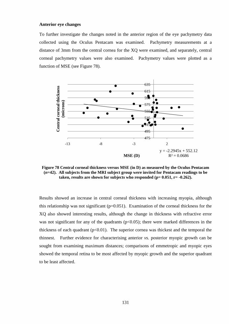
131

Anterior eye changes

To further investigate the changes noted in the anterior region of the eye pachymetry data

collected using the Oculus Pentacam was examined. Pachymetry measurements at a

distance of 3mm from the central cornea for the XQ were examined, and separately, central

corneal pachymetry values were also examined. Pachymetry values were plotted as a

function of MSE (see Figure 78).

Figure 78 Central corneal thickness versus MSE (in D) as measured by the Oculus Pentacam

(n=42). All subjects from the MRI subject group were invited for Pentacam readings to be

taken, results are shown for subjects who responded (p= 0.051, r= -0.262).

Results showed an increase in central corneal thickness with increasing myopia, although

this relationship was not significant (p=0.051). Examination of the corneal thickness for the

XQ also showed interesting results, although the change in thickness with refractive error

was not significant for any of the quadrants (p<0.05); there were marked differences in the

thickness of each quadrant (p<0.01). The superior cornea was thickest and the temporal the

thinnest. Further evidence for characterising anterior vs. posterior myopic growth can be

sought from examining maximum distances; comparisons of emmetropic and myopic eyes

showed the temporal retina to be most affected by myopic growth and the superior quadrant

to be least affected.

y = -2.2945x + 552.12

R² = 0.0686

475

495

515

535

555

575

595

615

635

-13 -8 -3 2

Cen

tra

l co

rnea

l th

ick

nes

s

(mic

ron

s)

MSE (D)

132

500

550

600

650

700

750

800

-11 -9 -7 -5 -3 -1 1 3

Co

rnea

l th

ick

nes

s (m

icro

ns)

MSE (in D)

Nasal

500

550

600

650

700

-11 -9 -7 -5 -3 -1 1 3

Corn

eal

thic

kn

ess

(mic

ron

s)

MSE (in D)

Temporal

500

550

600

650

700

750

800

-11 -9 -7 -5 -3 -1 1 3Co

rnea

l th

ick

nes

s (m

icro

ns)

MSE (in D)

Superior

133

Figure 79 Corneal thickness values (in microns) for the XQ, obtained using the Oculus

Pentacam (n=40)

9.7 Discussion and conclusions

Initially the findings placed focus on the inter-refractive group differences in the posterior

25% of the eye. The myopes showed gradual steepening of radius of curvature in the

posterior regions; in contrast both emmetropes and hyperopes displayed relative flattening.

The shape characteristics noted in the posterior eye agree with previous reports of a more

prolate, or less oblate, eye shape in myopes compared to emmetropes (Atchison et al. 2005;

2004; Logan et al. 2004). Of particular note is the area preceding the posterior changes,

where a more spherical shape was found. Greater irregularity in eye shape was also noted in

both low myope and emmetrope subject groups compared to high myopes. Irregularities in

eye shape have been previously noted in data collected using peripheral refraction

techniques (Tabernero & Schaeffel 2009).

The anterior eye was found to be similar between refractive groups in terms of radius of

curvature and ocular volume. The ocular volume results mirrored those of an earlier study

carried out using the same technique (Gilmartin et al. 2008). Corneal volume was measured

using the Oculus Pentacam and was also found to be similar between refractive groups.

To examine ocular shape in further detail, retinal quadrant shape differences were evaluated.

Initially chord differences between quadrants were examined. The results showed a great

deal of asymmetry in the anterior regions of the eye; a region which had thus far been

500

550

600

650

700

750

-11 -9 -7 -5 -3 -1 1 3

Co

rnea

l th

ick

nes

s (m

icro

ns)

MSE (in D)

Inferior

134

regarded as homogenous across refractive groups. Anteriorly, the nasal chord was larger

than the temporal (at a position approximately 15% along the distance of the presumed

visual axis). The quadrant asymmetries reduced up to the 75% mark, beyond which

increased disparity between quadrant chord lengths recommenced. In the vertical meridian

the inferior chord, in general, was larger than the superior. At the 75% mark there was a

larger dissimilarity between the superior and inferior chords for both myopic and hyperopic

eyes. These findings would suggest that despite the presence of many inter refractive group

similarities for the anterior ocular shape, pronounced quadrant dissimilarities exist. The

results will be affected, to a small degree, by the discrepancies between the visual and optic

axes. At the 75% mark all the differences in chord length appeared to be at a similar level

between refractive groups i.e. the graphs show the data from each refractive group intersect

in this region. The apparent similarity between refractive groups at the 75% mark once

again highlights the 75% region as a critical site in refractive error development.

Using a modification of an earlier experiment (Nagra et al. 2009) the maximal distances

from the presumed visual axis to the retinal surface were measured for each of the quadrants.

The largest maximum distance was noted in the superior quadrant (XQ) and ST (+Q); this

was the case for all refractive groups. Maximum distance values for the nasal quadrant were

noted as being the smallest for all refractive groups. Comparisons of maximum values in

high myopes vs. all other refractive groups showed particular enlargement of the temporal

quadrant, however, these findings did not reach statistical significance. The differences in

temporal growth compared to less myopic groups are noted in even low myopes. Multiple

reports have cited the temporal retina as being the most common site for retinal

degenerations associated with myopia e.g. retinal detachments and retinal holes (Shukla et

al. 1986). It is speculated that the temporal quadrant may possess some form of structurally

or sensory driven weakness, which ultimately exposes the temporal retina as a vulnerable

site for mechanical myopic stretch.

After establishing that there were both anterior and posterior inter refractive group

differences in eye shape, the study focused on the curvature, or bulbosity, of quadrants. The

coefficient for the 25-75% region revealed few refractive group differences, there were

however significant quadrant differences. The results demonstrated that although quadrants

were different in shape, this was not generally a consequence of refractive error. Greatest

variations were expected in the posterior 25% cap, however it was considered that 2nd

order

polynomial curve fits would not be able to accurately represent the data in this region,

135

therefore as an alternative respective meridians were examined (N-T, S-N, SN-IT, and ST-

IN). The meridional differences were not found to be significant across refractive groups; it

is acknowledged that combining two quadrants to produce a meridian may have masked

quadrant differences.

Inter eye differences produced interesting results showing differences in both the anterior

and posterior regions of right and left eyes and specific quadrant differences. While some

quadrants were noted as being different between eyes other quadrants were far more

homogenous. These differences can either indicate a physiological difference between the

right and left eyes or indicate a natural variation between eyes of the same individual.

Previous literature has described three models of eye shape; global expansion, equatorial

growth, and posterior pole elongation (Atchison et al. 2004; 2005; Strang et al. 1998). The

results from the current study indicate that a combination of these models best describes the

data. Posterior pole elongation has been associated with increasing myopia and the results

clearly indicate that myopic eyes are larger in size. Many reports have shown that myopic

eyes tend to have prolate, or less oblate, shaped eyes compared to emmetropes (Atchison et

al.2005; Stone & Flitcroft 2004). The posterior pole model illustrates the relative steepening

of myopic eyes in the posterior region and the radius band findings are in agreement with

this model. The variations in the more anterior region of the eye suggest that global

expansion models are not applicable to this region. Subtle quadrant differences in eye shape

are overlooked by these simplistic models. Additionally, further evaluation of the data is

required to assess the anterior regions of myopic eyes; MRI can be used in conjunction with

data collected with the Oculus Pentacam to provide more accurate descriptions of anterior

eye shape. Measures of anterior structures such as the crystalline lens and anterior chamber

will provide further understanding and help create models of the more anterior regions of the

eye in myopia.

9.8 Summary

In conclusion, there are significant differences in the size of myopic, emmetropic and

hyperopic eyes. Eye shape in the anterior sections of the eye is similar between refractive

groups, although subtle quadrant differences have been noted. In the posterior eye

meridional differences are not significant between refractive groups. Quantifying the

differences between quadrants in the posterior eye is challenging due to the discrepancies in

136

the optic and visual axes. The maximum distances for the superior-temporal and the

superior quadrants are largest relative to other quadrants for all refractive groups, and the

temporal quadrant appears to be most affected by myopic growth (see Figure 61). It is

envisaged that future analysis of the data will use engineering techniques such as finite

element analysis and mathematical modelling in order to quantify the change between

emmetropic eyes and myopic eyes.

Pages 137 and 138 have been removed for copyright restrictions.

139

11 PERIPHERAL REFRACTION AND OCULAR SHAPE

11.1 Introduction

Research in the field of peripheral refractive error has enjoyed renewed interest in recent

years due to the proposal that the peripheral retina mediates central structural development

of the eye (Wallman & Winawer 2004). In the 1970s a series of major studies concluded

that emmetropic subjects who subsequently developed myopia had been shown to possess

peripheral refractive errors which were hyperopic relative to the central refractive error

(Rempt et al 1971). The finding of a hyperopic periphery, relative to the fovea, in myopia

has been reported many times since (Seidemann et al 2002; Logan et al 2004; Calver et al.

2007).

The reasons why myopic development takes place in the presence of a hyperopic periphery

have been less well explored. In animal studies, occlusion of an eye generally causes

enlargement of the globe and thus myopia, that is, form deprivation myopia. It has been

suggested that as the eye cannot ‗see‘ a blurred image in front of the retina, the eye assumes

the image must lie behind it i.e. the eye believes it is too small and has a hyperopic refractive

error; the eye consequently grows to compensate for the presumed refractive error and can

be thought of as ‗searching‘ for a clearer image (Wallman & Winawer 2004). The

compensatory growth can also be shown through the use of negative powered lenses which

defocus the image and move it to a position behind the retina. Evidence for this reactive

growth in animals can be gained from measuring the changes in choroidal thickness in form

deprived animal eyes, where the introduction of a positive lens moves the images anterior to

the retina, and in an attempt to slow down growth the choroid thickens moving the retina to a

more anterior position. Conversely, the introduction of a negative powered lens moves the

image posterior to the retina, and the choroid becomes thinner in an attempt to move closer

to the image (Wallman & Winawer 2004).

Form deprivation can also lead to ocular enlargement in humans (O‘Leary & Millodot 1979;

Twomey et al. 1990). The eye is unable, however, to exercise exact homeostatic control and

prevent myopia from developing in otherwise healthy eyes. There has been a suggestion that

perhaps each individual has their own specific default refractive error setting which acts as a

‗STOP signal‘ to growth, i.e. an individual with a default setting of -3 dioptres may regulate

growth about this level of defocus, not allowing the eye to become more myopic or

140

emmetropic. The STOP signals may be cellular, biochemical or molecular based (Morgan &

Megaw 2004).

The theory that a hyperopic periphery drives myopic growth is explained in similar terms to

the reasons explaining form deprivation myopic growth. The relatively hyperopic region is

believed to send growth signals to the relatively myopic centre and stimulate axial growth

(Wallman & Winawer 2004). Therefore a relatively hyperopic peripheral refraction may act

as a predictor of future myopia onset and development (Rempt et al 1971).

11.2 Peripheral astigmatism

Ferree and Rand (1933) stated that it may be possible to calculate retinal contour from

peripheral refraction. With increasing eccentricity from the visual axis there is a

simultaneous variation in low level off axis aberrations; particularly peripheral astigmatism.

Consequently a peripheral refraction measurement cannot be directly converted into its

equivalent dioptric length in order to represent ocular shape and size; all refractive

components must be taken into account. Peripheral astigmatism and refractive error has

been modelled in schematic eyes in an attempt to derive retinal contour (Dunne et al. 1987).

Dunne et al. (1995) devised a computational approach for calculating retinal contour from

peripheral refraction taking account of crystalline lens thickness, corneal curvature, anterior

chamber depth and axial length. The program has been well established and has been used

to measure retinal contour in a number of studies (Dunne et al 1995; Logan et al 2004).

Although peripheral refraction techniques can provide a useful tool for retinal contour

calculation, their validity has been questioned (Stone & Flitcroft 2004). As the posterior

globe is particularly vulnerable to structural changes in myopia, it is imperative to the

understanding of myopic development that accurate assessments of eye shape in this region

can be made.

Three-dimensional MR imaging of the eye is a relatively new technique (Singh et al. 2006)

which has thus far not been compared to peripheral refractive techniques used to derive eye

shape. To evaluate whether the two techniques are comparable and interchangeable, the

current study sets out to compare data from subjects who have undergone both procedures.

If peripheral refraction is found to be an accurate and precise measure of retinal contour it

will possess several advantages over the MRI method. Costs of carrying out peripheral

refraction are much lower than MRI; a trained technician is able to carry out peripheral

141

autorefraction, whereas MRI requires qualified radiographers. Equipment and scan costs are

significantly greater for MRI scanning than autorefraction. Additionally, there are many

possible reasons why a subject may be unable to undergo MRI scanning; e.g. dental work,

metal implants or claustrophobia. In contrast, the autorefractor has very few procedural

limitations.

142

11.3 Purpose

The purpose of this study is to evaluate the differences between using the peripheral

refraction technique to derive retinal contour and contour derived from 3 dimensional ocular

MRI.

11.4 Hypothesis

It is hypothesised that measurements of retinal contour derived from peripheral refraction

will be contiguous with those found using MR imaging of ocular shape

11.5 Instrumentation

The Shin Nippon SRW 5000 IR binocular free space autorefractor was used to take

peripheral refractive measurements at 5˚ intervals up to a maximum of ±30˚ nasal and

temporal. Measurements were taken to the nearest 0.12D at a vertex distance of 12mm. The

Shin Nippon has been used extensively in peripheral refraction research. It has shown to be

highly repeatable and demonstrated a high level of accuracy through correlation with

subjective refraction (Mallen et al. 2001). A more comprehensive review of the Shin Nippon

autorefractor is detailed in the Chapter 7.

11.6 Methods

Forty two unpaid volunteers with refractive errors ranging from -10.56D to +4.38D

underwent peripheral refractive measurements, which were taken at 5˚ intervals up to a

maximum of 30˚ in the horizontal meridian. Subjects with astigmatic error greater than -

2.00D were excluded. The majority of subjects were either undergraduate Optometry

students or qualified optometrists, with ages ranging from 18 years to 40 years. Subjects

comprised of 30 females and 12 males. All subjects (bar one) had previously undergone the

ocular MRI. In addition to peripheral refractive and MR measurements, ocular biometric

components were measured using the Zeiss IOL Master (see section 7.3). Keratometry, axial

length measurements and anterior chamber depth recordings were used to facilitate the

calculation of retinal contour. Lens thickness was derived from the regression equation

reported by Smith et al. 2009. Informed consent was obtained from all volunteers prior to

the study.

143

To minimise the effect of accommodation 1 drop of 1% tropicamide ophthalmic solution

(Minims®, Bausch and Lomb Limited, Surrey, U.K) was instilled into each eye

approximately 25 minutes prior to autorefraction. The tropicamide also helped facilitate the

peripheral refraction readings by increasing the pupil size and enabling the measurement of

more peripheral readings, however some subjects responded less well to the dilating effects

of tropicamide and thus more peripheral measurements were difficult to obtain. Intraocular

pressures were measured before and after the experiment with non contact tonometery, and

verbal advice given in case of ocular adverse reactions to the tropicamide.

Subjects were positioned on the Shin Nippon autorefractor by use of an adjustable chin rest

and head rest. A custom designed and built extendable arm with a fixation target was

affixed to the autorefractor (see 7.2). The subject was then asked to fixate on a target at a

distance of approximately 1m, and a minimum of four readings at each angle were

attempted. The Shin Nippon autorefractor relies upon a focused image of the corneal mires

in order to take a measurement; for the more extreme peripheral measurements, corneal

curvature and pupil size restricted the number of readings. In some subjects measurements

up to 30˚ were not achievable.

11.7 Results

The spherical-cylindrical outputs from the autorefractor were converted into vector

components through use of equations developed by Thibos et al. (1997), these equations

have also been used by Atchison et al. 2006 and Calver et al. 2007 in their respective

analyses of peripheral refraction data.

The first equation calculates mean spherical error (MSE) using the standard equation:

MSE = Sph Cyl

2

Where MSE =Mean Spherical Error

Sph = Spherical error

Cyl = Cylindrical error

144

The second equation calculates the vector component J180 which is astigmatic error with an

axis between 90˚-180˚:

J180 = Cyl cos 2

2

The third equation calculates the astigmatic vector component J45 which is astigmatic error

with an axis that lies between 45˚-135˚:

J45 = Cyl sin 2

2

Calver et al. 2007 discuss a fourth equation to help recover the magnitude of astigmatism;

which takes the mean value of the three previous equations:

C‘ = 2 (J452 J180

2 )

Consistent with previous studies the reading 15˚ temporal to the fovea was removed as it is

the likely location of the optic disc (Atchison, 2006). Subject data were grouped according to

central mean MSE group. MSE results for each eccentricity were then compared between

refractive groups. Polynomial fits of J180 and linear fits of J45 helped describe the

relationship between refractive groups and the orientation of the astigmatism. Measures of

J180 and J45 were then used to calculate the cylindrical component (C‘).

Retinal contour was then derived by use of the computational program by Dunne et al.

(1995), RetinaFit. The program calculates retinal contour using formulae derived from

schematic eyes. There are three separate sections to the program; calculating tangential

corneal radius, sagittal refractive error and the interval of sturm; then entering data for each

eccentricity into the main retinal contour program. The program adjusts the corneal conic

constant values until they match the peripheral astigmatic value. The calculated sagittal

refractive value is then adjusted to match the measured value. Both adjustments require

manual manipulation. For each angle of eccentricity RetinaFit generates X and Y

coordinates. X and Y^2 coordinates are then used to derive curve fit estimates using a

statistical software package (SPSS version 16). From the quadratic curvature estimates,

values for the apical radius (r) and conic constants (p) are generated using the formula:

145

Y=AX X

where r = A/2

and p= -B (Dunne 1995).

The values r and p are inputted into the equation:

y = 2rx px

Previous literature cites fixed x values which correspond to each field angle (Dunne, 1995).

These values for x were inputted into the equation to calculate values for y. These figures are

based on schematic eyes and thus introduce a level of error for actual field angle being tested

(see Table 9); however the objective of the study was to compare the two techniques so for

this reason fixed values of x were used for both peripheral refraction and MRI techniques to

produce a direct comparison of techniques. For comparison purposes, the same

methodology was used on the MRI data to calculate r and p values. Again fixed x values

were used for the MR data to derive the y coordinate using the equation above.

X coordinate Field angle (°)

0.35 10

1.38 20

2.99 30

5.05 40

7.37 50

9.75 60

Table 9 The approximate distance from the fovea towards the anterior eye in millimetres which

would correspond to each field angle using a schematic eye (after Dunne, 1995)

The program is not significantly affected by inherent ocular errors such as crystalline lens

asphericity or changes in lens gradient index (Dunne 1995).

The differences between the MRI calculated y values and RetinaFit technique derived y

values were taken at each of the tested eccentricities. The mean differences for each subject

were plotted graphically to display the disparity between the two techniques.

In the current study the primary interests were:

I. The presence of relative peripheral hyperopia in myopic eyes

II. The correlation of retinal contour based on peripheral refraction with that

based on MRI.

146

For these reasons results from J180, J45, and C‘ data is included for completeness only, and

not explored in depth.

MSE

Subjects were placed into one of three groups based on MSE:

High myopes (greater than 6D myopia)

Low myopes (myopia between-6D and -0.5D)

Emmetropes (>-0.5≤ 1.75D).

Hyperopic subjects were excluded from this study due to insufficient subject numbers (n=2).

A summary of the average refractive errors and standard deviations are shown in Table 10

below. Right and left eyes were examined separately.

Refractive group Eye Average MSE Standard deviation

High myopes (n=6) Right -8.42 ±1.33

High myopes (n=7) Left -7.45 ±1.13

Low myopes (n=13) Right -2.39 ±1.53

Low myopes (n=13) Left -1.82 ±1.23

Emmetropes (n=22) Right +0.19 ±0.60

Emmetropes (n=20) Left +0.20 ±0.51

Table 10 The average MSE in dioptres (D) and standard deviations for each refractive

category, right and left eyes

The average MSE and corresponding standard deviations for each eccentricity are listed in

Table 11 for right and left eyes.

Eccentricity High myopes Low myopes Emmetropes

30n -6.17±3.78 -1.02±1.84 -0.01±1.32

25n -7.07±3.02 -1.85±2.19 0.22±1.04

20n -8.08±2.18 -2.09±2.11 0.29±0.77

15n -8.37±2.23 -2.43±2.02 0.16±0.89

10n -8.48±1.42 -2.49±1.82 0.23±0.65

147

5n -8.37±1.58 -2.48±1.94 0.20±0.69

0 -8.42±1.33 -2.39±1.53 0.19±0.59

5t -8.24±1.59 -2.54±1.57 0.18±0.56

10t -8.15±1.87 -2.60±1.56 0.09±0.57

20t -7.38±2.18 -2.50±1.93 -0.25±0.92

25t -5.71±2.66 -2.33±1.68 0.12±1.13

30t -2.90±0.57 -0.61±1.30 -0.13±0.89

Table 11 Mean MSE at each eccentricity for right eyes, for each refractive group ± standard

deviations (n= nasal retina, t= temporal retina). Results for eccentricity 15 degrees temporal

were omitted due to effect of the optic nerve head.

In general, most data were not normally distributed in accordance with the Kolmogorov-

Smirnov and Shapiro-Wilks tests of normality, therefore non parametric tests were employed

throughout.

The Kruksal Wallis test showed the three refractive groups were significantly different in

MSE at each eccentricity (p<0.001), except the temporal 30°. The lack of significance at

temporal 30° may be due to the limited number of readings taken at this point; results for this

eccentricity should therefore be treated with caution.

Post hoc tests were carried out using Mann Whitney U tests to compare peripheral MSE at

each eccentricity with central MSE. Critical values of significance were therefore reduced to

0.05/3=0.0167 (i.e. Bonferroni correction). Differences between emmetropes and low

myopes were significant at all eccentricities (p≤0.002), bar the temporal 30 and nasal 30

degrees. Differences between emmetropes and high myopes were significant at all

eccentricities (p≤0.001) bar temporal 30 degrees. Differences between low and high myopes

were significant at all eccentricities (p≤0.008) bar temporal 30 and temporal 25 degrees.

148

Figure 80 Graph of the mean uncorrected peripheral refractive error for right eyes fitted with

2nd

order polynomial curves (references to nasal and temporal refer to retinal not field

locations, n=42)

Relative difference in peripheral MSE compared to central MSE

To assess the amounts of relative hyperopia or myopia in the peripheral retina for each

group, the difference between the central MSE and MSE at each eccentricity for each

individual was calculated. The mean values for each refractive group were compared.


30n 2.61±2.60 1.12±1.45 -0.27±1.48

25n 1.63±1.97 0.67±1.27 0.03±1.10

20n 0.34±1.11 -0.30±1.11 0.10±0.64

15n 0.05±1.10 -0.04 ±0.79 -0.03±0.59

10n 0.06±0.53 -0.10±0.74 0.04±0.30

5n 0.05±0.55 -0.09±0.56 0.01±0.29

5t 0.18±0.56 -0.15±0.41 -0.01±0.25

y = 0.0016x2 - 0.0024x - 2.7013

R² = 0.7417

y = 0.0041x2 + 0.0367x - 8.7252

R² = 0.9073

y = -0.0002x2 - 0.0043x + 0.1808

R² = 0.5161

-10

-9

-8

-7

-6

-5

-4

-3

-2

-1

0

1

-40 -20 0 20 40

MS

E i

n D

Angle of Eccentricity (in degrees)

Low myopes

High Myopes

Emmetropes

Nasal Temporal

149

10t 0.27±0.58 -0.28±0.68 -0.09±0.35

20t 2.27±2.57 -0.18±1.12 -0.46±0.92

25t 2.99±2.06 -0.19±1.41 -0.08±1.18

30t 4.81±1.50 +1.53±2.50 -0.06±1.06

Table 12 Mean difference in MSE between central and peripheral locations, right eyes

Figure 81 Graphical representation of the mean difference in MSE between central and

peripheral locations, right eyes (linear fit used for emmetropic group, 2nd

order polynomials for

myopic groups)

Wilcoxon signed ranks test was used to compare the difference in MSE at each eccentricity

to the centre. The low myopic group showed a significant increase in hyperopia at nasal 30

degrees. High myopia showed significant differences in the temporal 20 and 25 degrees in

MSE relative to the central MSE. In emmetropic subjects, the only significant difference

between the central MSE and peripheral MSE was for temporal 30 degrees (p≤0.05).

Overall between groups there was a significant effect (found using the Kruksal Wallis test)

at temporal 20, 25 degrees and nasal 30 degrees which on post hoc testing (Mann Whitney

U) showed differences between the emmetropes and high myopes at all three eccentricities

and between low and high myopes at 25 degrees. There were no significant differences

y = 0.0015x2 - 0.0048x - 0.373

R² = 0.7069

y = 0.0042x2 + 0.0353x - 0.2318

R² = 0.9782

y = -0.0015x - 0.0643

R² = 0.0345

-1.00

0.00

1.00

2.00

3.00

4.00

5.00

-40 -30 -20 -10 0 10 20 30 40

Dif

fere

nce

bet

wee

n c

entr

al a

nd

per

iph

era

l

mea

n M

SE

(in

D)


Low Myopes

High Myopes

Emmetropes

Nasal Temporal

150

between emmetropes and low myopes in the degree of relative hyperopic or myopic defocus

in the periphery.

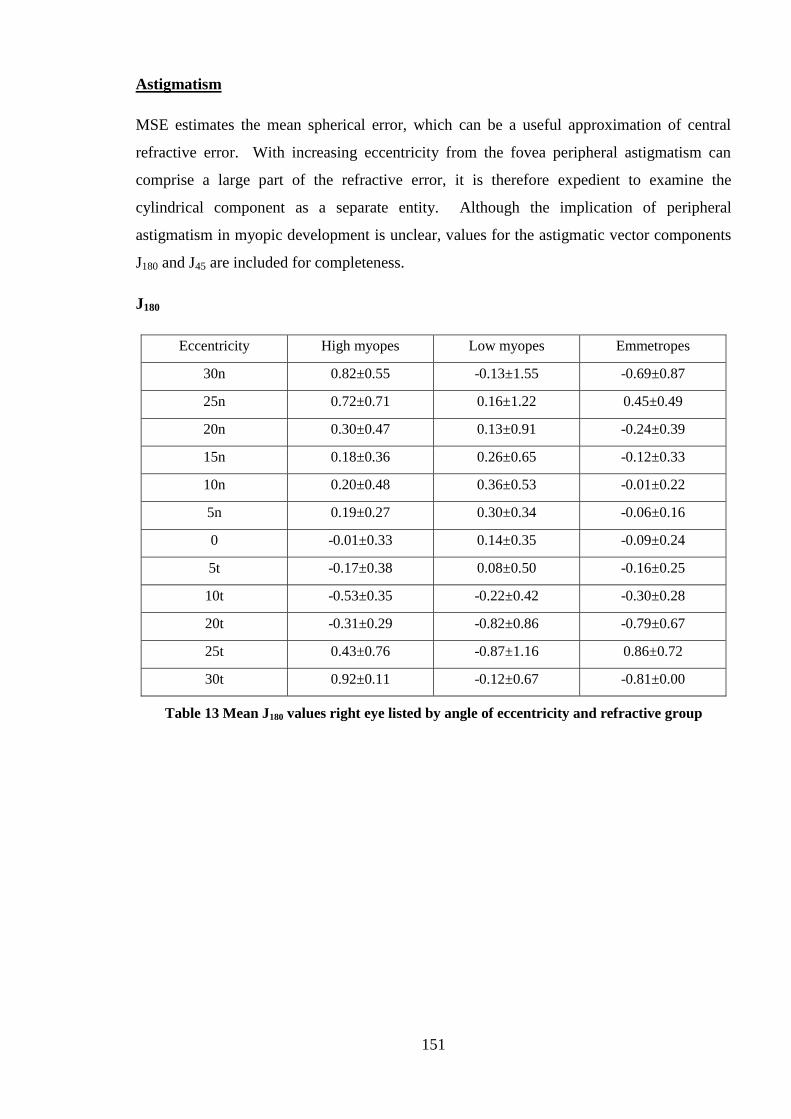
151

Astigmatism

MSE estimates the mean spherical error, which can be a useful approximation of central

refractive error. With increasing eccentricity from the fovea peripheral astigmatism can

comprise a large part of the refractive error, it is therefore expedient to examine the

cylindrical component as a separate entity. Although the implication of peripheral

astigmatism in myopic development is unclear, values for the astigmatic vector components

J180 and J45 are included for completeness.

J180


30n 0.82±0.55 -0.13±1.55 -0.69±0.87

25n 0.72±0.71 0.16±1.22 0.45±0.49

20n 0.30±0.47 0.13±0.91 -0.24±0.39

15n 0.18±0.36 0.26±0.65 -0.12±0.33

10n 0.20±0.48 0.36±0.53 -0.01±0.22

5n 0.19±0.27 0.30±0.34 -0.06±0.16

0 -0.01±0.33 0.14±0.35 -0.09±0.24

5t -0.17±0.38 0.08±0.50 -0.16±0.25

10t -0.53±0.35 -0.22±0.42 -0.30±0.28

20t -0.31±0.29 -0.82±0.86 -0.79±0.67

25t 0.43±0.76 -0.87±1.16 0.86±0.72

30t 0.92±0.11 -0.12±0.67 -0.81±0.00

Table 13 Mean J180 values right eye listed by angle of eccentricity and refractive group

152

Figure 82 Mean J180 values for right eyes, fitted with 2nd

order polynomial curves

Although not the main part of the study; J180 values were plotted for each refractive group as

a function of eccentricity (see Figure 82). The emmetropic and low myopic groups

displayed some nasal-temporal asymmetries; appearing to show higher levels of astigmatic

error in the temporal retina.

y = -0.0005x2 - 0.0128x + 0.0919

R² = 0.5513

y = 0.0011x2 - 0.0063x - 0.164

R² = 0.7017

y = -0.0008x2 - 0.007x - 0.1036

R² = 0.882

-1.50

-1.00

-0.50

0.00

0.50

1.00

1.50

-40 -30 -20 -10 0 10 20 30 40

J1

80

in

D


Low Myopes

High Myopes

Emmetropes

Nasal Temporal

153

J45


30n -0.13±0.37 -0.08±0.56 -0.23±0.42

25n -0.26±0.64 -0.08±0.42 -0.13±036

20n 0.01±0.62 0.01±0.33 0.16±0.35

15n -0.04±0.80 0.01±0.42 -0.02±0.36

10n 0.04±0.47 -0.17±0.36 -0.01±0.24

5n 0.03±0.29 0.01±0.42 -0.04±0.14

0 0.02±0.42 -0.07±0.32 0.01±0.10

5t 0.04±0.41 0.03±0.42 0.06±0.15

10t 0.29±0.74 -0.13±0.31 0.10±0.18

20t 0.34±0.64 -0.04±0.39 0.18±0.31

25t 0.38±0.94 0.06±0.54 0.22±0.34

30t 0.22±0.27 -0.08±0.39 -0.78±0.00

Table 14 J45 right eye, listed by angle of eccentricity and refractive group

154

Figure 83 Mean J45 values for right eyes, fitted with linear trend lines

Consistent with previous reports the nasal retina tended to show a greater degree of J45

astigmatism (Calver et al. 2007).

y = 0.0005x - 0.0429

R² = 0.0169

y = 0.0086x + 0.0894

R² = 0.7921

y = -3E-05x - 0.0665

R² = 5E-06

-1.00

-0.80

-0.60

-0.40

-0.20

0.00

0.20

0.40

0.60

-40 -30 -20 -10 0 10 20 30 40

J4

5 i

n D


Low Myopes

High Myopes

Emmetropes

Nasal Temporal

155

Cylindrical component

The cylindrical component was derived as a measure of the magnitude of astigmatism at

each of the eccentricities. The cylindrical component is considered to be more useful than

J180 and J45 vector analysis as it provides information on magnitude of astigmatism rather

than reducing astigmatism into separate components and describing them separately (Thibos

et al 1997; Calver et al 2007).


30n -1.84±0.97 -2.84±1.41 -2.11±1.11

25n -1.95±1.37 -2.22±1.20 -1.35±0.70

20n -1.33±0.85 -1.65±0.92 -1.03±0.59

15n -1.46±-0.86 -1.54±0.60 -0.85±0.50

10n -1.17±0.62 -1.37±0.53 -0.57±0.32

5n -0.71±0.47 -1.06±0.59 -0.40±0.20

0 -0.89±0.44 -0.80±0.57 -0.45±0.30

5t -1.04±0.31 -0.97±0.85 -0.56±0.37

10t -1.73±0.93 -0.95±0.64 -0.80±0.42

20t -1.42±0.71 -1.94±1.55 -1.93±1.05

25t -2.22±1.16 -2.37±1.93 -1.75±1.33

30t -1.94±0.09 -1.27±0.69 -2.25±0.00

Table 15 Cylindrical component as calculated from vector components J180 and J45, right eyes

156

Figure 84 Graphical representation of cylindrical component, for right eyes only

Each of the refractive groups showed clear nasal-temporal asymmetry. The magnitude of

astigmatism varied significantly between groups in the central ~15° (p= <0.05, Kruksal

Wallis test), interestingly beyond this eccentricity there was not a significant difference in

amount of astigmatism between the three refractive groups.

-3.00

-2.50

-2.00

-1.50

-1.00

-0.50

0.00

-40 -30 -20 -10 0 10 20 30 40

Cy

lin

dri

cal co

mp

on

ent

(in

D)


Low Myopes

High Myopes

Emmetropes

TemporalNasal TemporalNasal

157

Retinal contour calculation through RetinaFit

Each subject‘s peripheral refractive measurements were inputted into the RetinaFit program

as described above, alongside their individual ocular biometric measurements. The

difference in the y coordinates was examined.

Each individual subject‘s MRI data was also analysed in the horizontal meridian. The data

for the distance 3mm either side of the fovea (nasal and temporal) was taken and plotted (see

Table 9). The distance along the axis was subtracted from the calculated total axial length to

derive a new set of axial length corrected values; these were then corrected to ensure 3mm

either side of the presumed foveal location was used. As with the RetinaFit procedure the

calculated x values and the y² values were inputted into a statistical package and quadratic

curve fit estimations derived; from this r and p values were calculated (see Methods).

Assuming the same x fixed values previously indicated the y coordinate was derived. The

difference between MRI and RetinaFit y values was taken and represented graphically (see

Figure 85).

Figure 85 The difference in retinal contour data as derived by MRI and RetinaFit by field

angle (combined average of n=41)

R² = 0.9451

-0.5

0

0.5

1

1.5

2

2.5

3

3.5

0 5 10 15 20 25 30 35Dif

fere

nce

bet

wee

n M

RI

an

d R

etin

aF

it d

eriv

ed y

va

lues

(M

RI

min

us

Ret

fit,

in

mm

)

Angle of eccentricity (in degrees)

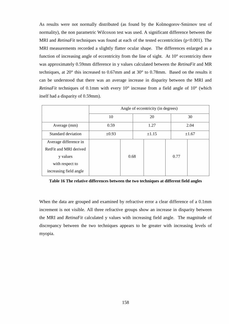
158

As results were not normally distributed (as found by the Kolmogorov-Smirnov test of

normality), the non parametric Wilcoxon test was used. A significant difference between the

MRI and RetinaFit techniques was found at each of the tested eccentricities (p<0.001). The

MRI measurements recorded a slightly flatter ocular shape. The differences enlarged as a

function of increasing angle of eccentricity from the line of sight. At 10° eccentricity there

was approximately 0.59mm difference in y values calculated between the RetinaFit and MR

techniques, at 20° this increased to 0.67mm and at 30° to 0.78mm. Based on the results it

can be understood that there was an average increase in disparity between the MRI and

RetinaFit techniques of 0.1mm with every 10° increase from a field angle of 10° (which

itself had a disparity of 0.59mm).

Angle of eccentricity (in degrees)

10 20 30

Average (mm) 0.59 1.27 2.04

Standard deviation ±0.93 ±1.15 ±1.67

Average difference in

RetFit and MRI derived

y values

with respect to

increasing field angle

0.68 0.77

Table 16 The relative differences between the two techniques at different field angles

When the data are grouped and examined by refractive error a clear difference of a 0.1mm

increment is not visible. All three refractive groups show an increase in disparity between

the MRI and RetinaFit calculated y values with increasing field angle. The magnitude of

discrepancy between the two techniques appears to be greater with increasing levels of

myopia.

159

Figure 86 Mean difference for y values between the MRI and RetinaFit techniques, with

reference to refractive error

Refractive group Angle of Eccentricity (in degrees)

10 20 30

Low Myopes 0.57±0.34 1.21±0.06 2.19±1.69

High Myopes 1.56±1.00 2.68±0.84 2.9±1.07

Emmetropes 0.39±1.31 0.92±1.56 1.77±0.10

Table 17 Mean differences in y values between the MR data and RetinaFit program values (in

mm)

0

0.5

1

1.5

2

2.5

3

3.5

0 5 10 15 20 25 30 35

MR

I m

inu

s R

etF

it (

y v

alu

e)


LM

HM

EMM

160


MSE and astigmatic components

Results for MSE and the astigmatic representations of the peripheral refraction data were

generally in line with previous reports (Calver et al. 2007; Atchison et al. 2006). Myopic

eyes generally showed hyperopic defocus at field angles away from the fovea; the hyperopia

appeared to increase with increasing eccentricity. The levels of hyperopic defocus only

became significant at more peripheral locations (i.e. 25° and beyond) compared to the central

MSE. Emmetropic eyes showed relative myopia in the periphery, but the disparity between

central and peripheral MSE was less pronounced compared with myopes. Furthermore the

highly myopic group appeared to show a more exaggerated effect i.e. more relative

hyperopia in the periphery, than the low myopes.

Consistent with previous reports J180 and J45 components appeared to show astigmatic error

for J180 to be greater in the temporal retina than nasal, and J45 to be greater in the nasal retina

(Calver et al 2007; Atchison et al. 2006). Also consistent with previous reports, the

differences between nasal and temporal retinae are more marked for the J180 component than

J45.

The magnitude of astigmatism varied between the nasal and temporal hemi-fields. In

general, the temporal retina showing greater astigmatism than the nasal. Similar nasal-

temporal asymmetries in astigmatism have been reported previously, (Seidemann et al 2002;

Dunne et al 1993).

Interestingly, the amount of astigmatism for the three refractive groups only varied

significantly in approximately the central 15°. Beyond the central region there were no

significant differences in the magnitude of astigmatism; this places further focus on the

spherical element of the Rx.

RetinaFit and MRI correlation

A unique aspect of this study was the correlation of the retinal contour generated from

peripheral refraction with the MRI ocular shape data. Results showed consistent differences

between the two techniques as a function of increasing field angle. Due to technical

difficulties with the program, which could not be resolved within the time scale of the

161

current study, a maximum retinal area of 30° only was covered. Once these technical

difficulties are resolved, the extent of the retina examined will depend upon the angles at

which peripheral refraction was measurable by the investigator. Overall, the MRI technique

estimated retinal contour to be flatter than the RetinaFit. The disparities between the results

increased as a function of increasing field angle. The relationship between the field angle

and error appeared to be linear when the cohort was not split by refractive group; increasing

at a rate of 0.1mm for every 10° increase in angle beyond 10°. Thus this error can be used to

develop a correction within the RetinaFit program. Examining the differences between MR

data and the RetinaFit program by refractive error did not show the same level of error;

therefore a 0.1mm correction factor would introduce its own level of error.

The present study has shown that laboratories using peripheral refraction methods as a

means of estimating retinal contour should treat peripheral field angle results with caution

owing to the discrepancies noted with increasing field angle.

There could be several causes for the differences in results derived from the two techniques;

in peripheral refraction the location of the line of sight is easily located through use of the

Shin Nippon autorefractor. In MR imaging, locating the visual axis is more problematic (see

9.2.3). The difference between the optic axis (geometric axis) and visual axis is termed

angle α. There is both a horizontal, and of less significance, vertical element to angle α.

MRI images are taken along the nominal optic axis.

Additionally, MR imaging is not affected by optical refractive components, whereas

peripheral refraction is vulnerable to refractive component properties such as changes in

refractive index, curvature of refractive components and errors in autorefractor

measurements. Although lens tilt and optical component displacement do not significantly

affect the RetinaFit program, it is likely that other aberrations will affect the results.

As the differences between the y values calculated from MRI data and RetinaFit appear to be

linear for refractive groups as a whole, a correction could be applied to the RetinaFit

program to make values comparable to MR data. However, it must be stressed that

differences in the MR data and RetinaFit discrepancy exist as a function of refractive group.

Peripheral refraction possesses several advantages over the MRI technique, the main being

cost. MRI also potentially poses significant risk to volunteer subjects and a stringent set of

criteria must be met before subjects can undergo MR scanning. Furthermore retinal contour

162

measures derived through peripheral refraction are especially advantageous in paediatric

ocular research, as the requirement for good fixation for MR scanning can be overcome.

11.9 Summary

In conclusion, the results from the MSE, J180, J45 measures are consistent with those reported

previously. The study has examined a unique application of peripheral refraction derived

retinal contour by correlating it with MRI derived retinal contour. The results indicate that

there is some scope for transforming RetinaFit data to generate retinal contours that match

approximately those generated by MRI.

163

12 VISUAL FIELD SENSITIVITY AND OCULAR SHAPE

12.1 Introduction

Visual field testing is a commonly used technique by practitioners to assess peripheral visual

function in clinical optometric practice and hospital settings. The test involves determining

sensitivity to light at multiple locations in both the central and peripheral retina; the

responses are derived from the cone photoreceptor pathway. Visual field testing has shown

reduced sensitivity in myopic subjects (Martin-Boglind, 1991; Aung et al. 2001; Rudnicka

and Edgar 1995). Loss in sensitivity may occur at levels of myopia as low as -2D±1D

(Czepita and Chmielewska, 2004). In particular the superior temporal field (inferior nasal

retina) has been reported to show reduced sensitivity (see 4.4). Although the source of a

reduced sensitivity is unclear, there are several possibilities. Decreased retinal luminance

due to a longer axial length; changes in the photoreceptor cells; decreased photoreceptor

density as a consequence of ocular expansion (Rudnicka and Edgar, 1995); misdirection or

misalignment of photoreceptors caused by an increased in axial length, or pathological

fundus changes may all contribute to a reduction in visual field sensitivity.

To further explore the theory that ocular shape may affect the light sensitivity threshold,

specific indices of retinal curvature and shape derived from MR imaging analysis are

correlated with mean visual field thresholds from the corresponding retinal regions. It is

envisaged that in general larger eye sizes will correlate with reduced visual field sensitivity.

164

12.2 Purpose

The purpose of this study is to determine the relationship between retinal shape, specifically

the posterior 25% cap of the eye, with visual field sensitivity, using subjects from a range of

refractive error and age groups.

12.3 Hypothesis

Based upon the current literature, it is proposed that ocular expansion produces reduced

visual field responses possibly as a consequence of reduced photoreceptor density. It is

hypothesised that retinal quadrants which show greater expansion, as determined through

surface area and interval variance (IV) measurements, will correlate with a reduction in

visual field response.


The commercially available and widely used automated Humphrey Visual Fields Analyser

(HFA) was used to test visual field sensitivity (see 7.4). The SITA-Standard threshold

program within the HFA was used as an alternative to a full threshold fields program, due to

its ability to yield results comparable to full threshold testing in a fraction of the time. The

SITA Standard program also helped simulate a typical clinical setting and aided in

combating the effects of fatigue by providing a shorter test time. Previous studies of

automated perimetry in myopic subjects have shown the 30-2 single threshold test on the

Humphrey Visual Field Analyser as sufficient for screening purposes for pathology affecting

visual fields (Rudnicka and Edgar, 1995).

Two program settings were used: the 30-2 program, which tests locations within the central

60˚ field at 6˚ intervals and on a smaller subset of subjects; the central 10-2 program which

tests the central 20 ˚ field at 1˚ intervals. The 10-2 fields program improves the ability to

detect smaller areas of focal loss in the central field.

12.5 Methods

The cohort comprised of 40 young adult subjects for whom 3-dimensional ocular MR

images had been previously acquired. Ages ranged from 18-40 years old. Mean spherical

error (MSE) for the group ranged from -9.31D to +4.19D, and respective axial lengths from

165

27.64mm to 21.84mm. Subject refractive errors were obtained by use of the Shin Nippon

5000 autorefractor and axial length measurements were recorded using the Zeiss IOL Master

(see 7.2 and 7.3). Full refractive corrections were worn throughout all recordings, only

subjects with astigmatism under 2.00DC were included in the study to ensure most

ametropia was of spherical origin.

All subjects underwent central 30-2 SITA standard visual fields testing on the Humphrey

Visual Fields Analyser. Subjects were invited back to attend for a 10-2 SITA threshold

fields program test however response was poor with only 9 subjects returning. Ethical

consent was sought and all subjects were unpaid.

Monocular tests were carried out: right eyes were tested first, followed by the left eye. The

same order was maintained throughout the experiment, but for the purposes of analysis only

right eye data is presented. There were no significant differences between right and left eye

sensitivities (TD and MS) as determined by a paired student t-test.

Subjects were given a break for approximately ten minutes between each test; breaks were

also provided at the subject‘s request. Throughout the visual fields tests, subject fixation

was monitored via a fixation video monitor and also by the Humphrey machine‘s built in

Heijl-Krakau method of fixation monitoring. All tests with fixation losses above 20% were

rejected.

Mean maximum sensitivity (MS) values for each quadrant of the visual field were obtained

through averaging results using the orthogonal axes provided on the visual fields plot for XQ

quadrants (as defined in Chapter 9). For the +Q quadrants the plots were divided at 45° to

the orthogonal axes. To maximise inclusion of data, any point lying on the XQ axis was

included into the quadrant which lay directly anticlockwise (right eyes). The method is

detailed in the Figure 87.

166

Figure 87 The technique used to divide visual fields plots into quadrants. The greyed-out

regions show the position of the blind spot and the point directly above the blind spot, these two

points were excluded from analysis (as is standard in visual fields research). The circles show

the points which lie on the axes and the arrows show the quadrant into which these circled

points were included

167

Further measures of visual field function were obtained through use of age corrected total

deviation (TD) plots. The TD quadrant averages were obtained using the same method as

the numeric MS plots.

In order to compare visual field sensitivity values for each quadrant with ocular shape,

interval variance measurements (IV) were obtained by calculating the standard deviations for

the MR data comprising the posterior 25% of each quadrant and deriving the 95% IV (i.e.

1.96 * standard deviation). Further indices of shape were calculated by deriving the surface

area (SA) for each quadrant. The mean 2-dimensional data for the posterior 25% of each

quadrant were plotted graphically and fitted with second order polynomials (see 9.5). The

polynomial equations were then inputted into formulae for the calculation of surface area

(derived by Dr Bill Cox and Professor Bernard Gilmartin):

S=

6a2 1 3/2 1

S = surface area of posterior 25% cap

a = the ‗a‘ coefficient in y = ax2+c (from fitting the posterior 25% data for each quadrant

with a second order polynomial curve)

r = the x coefficient of the polynomial equation

Analysis was carried out through repeated measures ANOVAS, and ANCOVAS with age as

a covariate. Further investigations were carried out using linear correlations.

168

12.6 Results

Refractive error vs. axial length

Pearson‘s correlation coefficient showed refractive error to be correlated significantly with

axial length; the R2 value was consistent with previous studies.

Figure 88 The significant relationship between axial length (in mm) and mean spherical error

(MSE in D, n=40) (one tailed Pearson’s correlation coefficient p<0.001, r = -0.854)

Mean spherical error (MSE) ranged from +4.185D to -9.31D and axial lengths ranged from

21.84mm to 27.24mm.

Age vs. Visual fields sensitivity

As expected increasing age was significantly correlated with a decline in mean visual field

sensitivity (one-tailed Pearson‘s correlation coefficient p<0.05, r=-0.267).

Visual field sensitivity by quadrant

Maximum Sensitivity (dB)

Mean MS values for each quadrant are shown in Table 18.

y = -0.3461x + 23.58

R² = 0.7291

20

21

22

23

24

25

26

27

28

29

-12 -8 -4 0 4

Axia

l le

ng

th (

in m

m)

MSE (in D)

169

Figure 89 Graph showing the mean sensitivity for each of the XQ quadrants, error bars show

standard deviations

Repeated measures ANCOVA, with age as a covariate, showed significant differences

between the inferior vs. temporal, nasal and superior quadrants (p<0.01).

Figure 90 Graph showing the mean MS response for each of the +Q quadrants, error bars

show standard deviations

Repeated measures ANCOVA controlling for age showed significant differences between all

quadrants (p<0.01) bar inferior nasal vs. inferior temporal.

28.5

29

29.5

30

30.5

31

31.5

32

32.5

33

Nasal Superior Temporal Inferior

Mea

n s

en

siti

vit

y (

dB

)

Quadrant (retinal)

29

29.5

30

30.5

31

31.5

32

32.5

33

SN ST IT IN

Mea

n s

en

siti

vit

y (

dB

)

Quadrant (retinal)

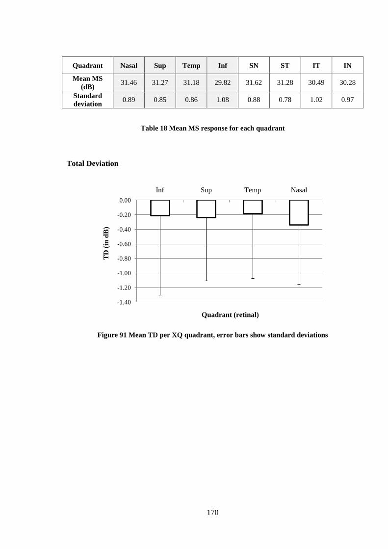
170

Quadrant Nasal Sup Temp Inf SN ST IT IN

Mean MS

(dB) 31.46 31.27 31.18 29.82 31.62 31.28 30.49 30.28

Standard

deviation 0.89 0.85 0.86 1.08 0.88 0.78 1.02 0.97

Table 18 Mean MS response for each quadrant

Total Deviation

Figure 91 Mean TD per XQ quadrant, error bars show standard deviations

-1.40

-1.20

-1.00

-0.80

-0.60

-0.40

-0.20

0.00

Inf Sup Temp Nasal

TD

(in

dB

)

Quadrant (retinal)

171

Figure 92 Mean TD per +Q quadrant, error bars show standard deviations

Repeated measures ANOVA showed there to be no significant differences between

quadrants for both XQ and +Q (p= <0.05).

Quadrant Temp Inf Sup Nasal

Mean TD

(dB) -0.19 -0.22 -0.24 -0.34

Standard

deviation 0.89 1.09 0.87 0.82

Table 19 Mean TD of responses for each XQ quadrant

Quadrant ST SN IT IN

Mean TD

(dB) -0.09 -0.24 -0.28 -0.34

Standard

deviation 0.79 0.80 1.01 0.99

Table 20 Mean TD of responses for each +Q quadrant

Axial length

Axial length was tested for correlation with MS, using a semi-partial correlation which

controlled for age. Axial length was not significantly correlated with MS responses for any

quadrant. TD was also checked for correlations with axial length using Pearson‘s correlation

coefficient; but no significant correlations were noted for any of the quadrants (p= <0.05).

-1.60

-1.40

-1.20

-1.00

-0.80

-0.60

-0.40

-0.20

0.00

IN IT ST SN

TD

(in

dB

)

Quadrant (retinal)

172

Retinal surface area

Mean retinal surface area for each quadrant, XQ and +Q are shown in the figures below:

Figure 93 Mean surface areas for each XQ quadrant are shown for the posterior 25% cap of

the eye. Error bars show standard deviations

Repeated measures ANOVA showed significant differences between the surface areas of the

nasal vs. superior and nasal vs. inferior quadrants (p=0.013 for both).

A semi-partial correlation with age as a covariate did not show a significant relationship

between MS and SA of corresponding quadrants (XQ) (p= <0.05).

Pearson‘s correlation coefficient did not show a significant relationship between TD and SA

(XQ).

0.00

50.00

100.00

150.00

200.00

250.00

300.00

Sup Inf Temp Nasal

PO

ST

ER

IOR

25%

SU

RF

AC

E

AR

EA

in

mm

²

Quadrant (retinal)

173

Figure 94 Mean surface areas for each +Q quadrant are shown for the posterior 25% cap of

the eye. Error bars show standard deviations

Repeated measures ANOVA did not show significant differences between surface areas of

+Q quadrants. A semi-partial correlation (controlled for age) did not show a significant

relationship between MS and SA of corresponding quadrants (+Q) (p= <0.05).

Quadrant Nasal Temporal Superior Inferior Sup-

temp

Inf-

nasal

Sup-

nasal

Inf-temp

Average

(mm²)

213.15 221.25 227.89 227.04 226.77 229.09 220.03 220.86

Standard

deviation

34.26 31.68 28.37 31.09 29.11 38.48 28.27 34.02

Table 21 Surface area values and standard deviations for each quadrant

Interval Variance (IV)

Mean retinal IV values are shown for each quadrant in Table 22.

0.00

50.00

100.00

150.00

200.00

250.00

300.00

IN ST IT SN

PO

ST

ER

IOR

25

% S

UR

FA

CE

AR

EA

in

mm

²

Quadrant (retinal)

174

Figure 95 IV indices per retinal quadrant, error bars show standard deviations

One way repeated measures ANOVA showed significant differences between all quadrants

(p<0.01) bar the nasal vs. inferior and temporal vs. superior.

A semi-partial correlation (controlling for age) showed a significant relationship between the

superior quadrant IV and MS (p=0.022, r=-0.365), although by using a Bonferroni correction

for four quadrants this would no longer be significant.

Pearson‘s correlation of TD and IV showed a significant relationship for the superior

quadrant (p = <0.001, r = -0.498).

Figure 96 IV per retinal quadrant, error bars show standard deviations

4.60

4.80

5.00

5.20

5.40

5.60

5.80

6.00

6.20

Temp Sup Inf Nasal

IV (

in m

m)

Quadrant (retinal)

4.6

4.8

5.0

5.2

5.4

5.6

5.8

6.0

6.2

ST IT SN IN

IV (

in m

m)

Quadrant (retinal)

175

Repeated measures ANOVA showed significant differences between all quadrants (p<0.01),

bar inferior-nasal vs. superior-nasal and superior-nasal vs. inferior-temporal.

A semi-partial correlation (controlling for age) showed a correlation between MS and IV for

the superior temporal quadrant (p=0.005, r= -0.445).

Pearson‘s correlation of TD and IV showed a significant relationship for the superior

temporal quadrant (p=0.002, r= -0.478).

Quadrant Nasal Temporal Superior Inferior Sup-

temp

Inf-

nasal

Sup-

nasal

Inf-

temp

Average

(mm)

5.07 5.61 5.60 5.18 5.76 5.04 5.20 5.38

Standard

deviation

0.34 0.40 0.38 0.30 0.35 0.29 0.53 0.30

Table 22 Mean IV values for each quadrant, based on MRI data for the posterior 25% of the

eye

12.6.1 Discussion and conclusions

Reduced photoreceptor density created by ocular expansion has been suggested as a cause of

reduced visual field sensitivity in myopic subjects. To investigate the effect of ocular shape

on visual field sensitivity, shape indices derived from magnetic resonance imaging data were

correlated with visual field sensitivity from corresponding retinal quadrants. Both maximum

sensitivity (MS) and total deviation (TD) plots were correlated with surface areas and

interval variance (IV). Correlations of surface areas with TD and MS failed to reach

significance; IV, however, was correlated with visual field sensitivity. Notably the superior

and superior-temporal TD and the superior-temporal MS were correlated with the IV. Based

on the results of the current study the relationship between ocular shape and visual field

sensitivity appears to be limited to the superior and superior-temporal quadrants only;

interestingly the superior-temporal quadrant has been widely implicated in myopia as a site

of myopic retinal damage. Retinal degenerations associated with myopic enlargement are

known to occur most frequently in the superior-temporal quadrant (Hyams et al. 1975;

Shukla and Ahuja, 1983).

176

The present study shows that although the significant correlations between eye shape and

visual field sensitivity are limited to just the superior-temporal and superior quadrants, a well

established inter quadrant variance exists. The inferior quadrant MS response was

significantly reduced compared to the nasal, superior and temporal quadrants. Furthermore

the inferior hemifields also showed reduced visual field sensitivity in the +Q.

Although the purpose of the experiment was to investigate ocular shape with reference to

visual field sensitivity, isolating the effect of shape alone is difficult. There are several

factors associated with shape: surface area, curvature, stretch, and photoreceptor distribution

and density. To accurately evaluate the relationship between ocular shape and visual field

sensitivity, determination of all the factors is required.

12.7 Summary

Although two quadrants did show a significant correlation between visual field sensitivity

and indices of ocular shape, in general it can be concluded that visual fields sensitivity and

ocular shape are not correlated.

177

13 MULTIFOCAL ELECTRORETINOGRAM AND OCULAR SHAPE

13.1 Introduction

Electrophysiological testing provides an objective method of quantifying the functional

changes in the retina. Most recently the multifocal electroretinogram (mfERG) has been

used to compare responses from myopic and emmetropic eyes; mfERG helps to provide

information about specific locations over the central 50° of the retina (see Figure 99). A

number of sources have cited the decline in mfERG response with a longer axial length

(Chan & Mohidin 2003), whilst others have attributed the reduced response to myopic

refractive error. As the two conditions often coexist it is difficult to control for the effects of

each, however, through use of ANCOVA analyses it has been suggested that axial length

may only be responsible for approximately 15% of the decline in response and refractive

error for 27% (Chen et al. 2006a). The remaining decline in response has been attributed to

numerous factors such as increased retinal cell spacing with myopic retinal stretch

(Kawabata & chi-Usami 1997) or damage to retinal cells as a consequence of retinal

expansion. Reports of mfERG investigation with reference to axial length and refractive

error have not been consistent; although the amplitudes or implicit times may be reduced in

myopic eyes there is still variation in the retinal location producing the reduced response.

Some reports have suggested loss originating from a central location whereas others a more

central and peripheral location (Kawabata & chi-Usami 1997). Additionally the reductions

in mfERG response appear to be limited to progressing myopes or high myopes; stable

myopes and emmetropes have been reported to produce similar responses (Chen et al.

2006a). In part the lack of consistency may originate from individual variations in cell

topography, but also differences in the protocols used by different laboratories. The

differences in protocols arise most frequently in the type of mfERG component analysed and

the type of stimulus. The mfERG produces a waveform response, and most often

researchers concentrate on the amplitude of the first peak (P1) and its implicit time (also

referred to as latency). Another widely assessed component is the amplitude and implicit

time of the first trough: N1. Additionally, further components of the mfERG waveform

response may be examined; investigations of the second trough (N2) and other smaller

secondary aspects of the response waveform have also been reported (Chen et al. 2006b).

Differences between laboratories have also arisen in the type of stimulus used. The stimulus

comprises a hexagonal pattern and there are three levels of stimulus: 61, 103, or 241

hexagons. If a smaller number of hexagons are used as a stimulus, a larger region of the

178

retina is represented by each hexagon. For detecting small retinal differences, a larger

number of hexagons is considered more favourable. The advantage of a larger number of

hexagons can be offset by the inaccuracies produced by fixation losses; if a small number of

hexagons are used, with each covering a larger retinal region, small eye movements could be

accommodated without loss of accuracy. For the purpose of this study a stimulus array of

103 hexagons is used to enable a small reduction in response to be detected without the

detrimental effects of small eye movements

Multifocal ERG is a difficult measurement to obtain; the signal is highly susceptible to

contamination from nearby electrical sources, blinking, movement or jaw clenching. As

subjects are required to fixate on a screen which displays a flashing stimulus for extended

periods of time, the probability of contamination through blinking is particularly high. To

reduce the commonly encountered artefacts many labs use software to ‗smooth‘ the data by

averaging the response with neighbouring hexagons. The use of this smoothing tool is

warned against by the International Society for Clinical Electrophysiology of Vision in their

standards for mfERG recordings as loss of information may occur. In the current study

subjects with high levels of contaminated data which were deemed unreliable were rejected;

therefore no smoothing was required.

Although the mfERG has been studied in reference to refractive error and axial length, thus

far results are inconsistent. It is unclear whether the mfERG response of myopic eyes is

affected by the retinal shape. In the present study in addition to carrying out analyses with

refractive error and axial length, analysis will also be carried out with reference to specific

indices of ocular shape namely Interval Variance (IV) and surface areas (see 9.5.5).

179

13.2 Purpose

To evaluate the relationship between ocular shape and multifocal electroretinogram

responses.

13.3 Methods and instrumentation

Twenty three young adult subjects of good ocular health underwent standard mfERG

recordings. Subjects were divided by refractive error; the cohort comprised of 12 myopes

and 11 emmetropes. Mean refractive errors were -4.63±3.2D for the myopes and -

0.03±0.31D for the emmetropes, mean PCI axial length measurements were 25.32±1.20mm

for myopes and 23.48±0.45mm for emmetropes. The left eyes of each subject were

examined. Left eyes were selected on the basis that the preliminary data had shown the right

eyes to possess greater signal contamination and interference (possibly due to the positioning

of electrical equipment in the lab). Informed consent was obtained from all subjects and all

undergraduate subjects were paid a small fee for attendance. All recordings were carried out

with the advice and guidance of experienced electrophysiologists, Andrea Scott and Dr Ian

Fawcett.

Left eye monocular multifocal recordings were carried out using the VERIS System (VERIS

Electro-Diagnostic Imaging, Inc.CA, USA), the right eye was occluded. All recordings were

repeated in order to obtain an average of two readings, in 2 cases a repeat was not possible

owing to either poor fixation, subject discomfort or machine error. A Dawson-Trick-

Litzkow (DTL) thread electrode was used to detect the response. DTL fibres provide

increased comfort compared to contact lens electrodes (Dawson et al 1979) and are therefore

less likely to produce blink artefacts. Intraocular pressure readings and anterior chamber

readings were obtained prior to the instillation of 1% tropicamide ophthalmic solution

(Minims®, Bausch and Lomb U.K Limited, Surrey, U.K). Intraocular pressures were also

measured post dilation, using a standard commercially available non contact tonometer. All

subjects were given advice regarding the side effects of tropicamide.

An abrasive paste was used to clean subjects skin in preparation for the grounding and active

electrodes. The cleaning helped minimise skin oils which may otherwise have disturbed the

transmission of signals and recordings. In addition to the corneal electrode, gold cup

electrodes were attached on the left ear lobe and forehead. Conductive gel (NuPrep® gel,

Weaver and Company) was used in the gold cup electrodes to allow improved transmission

of the signal.

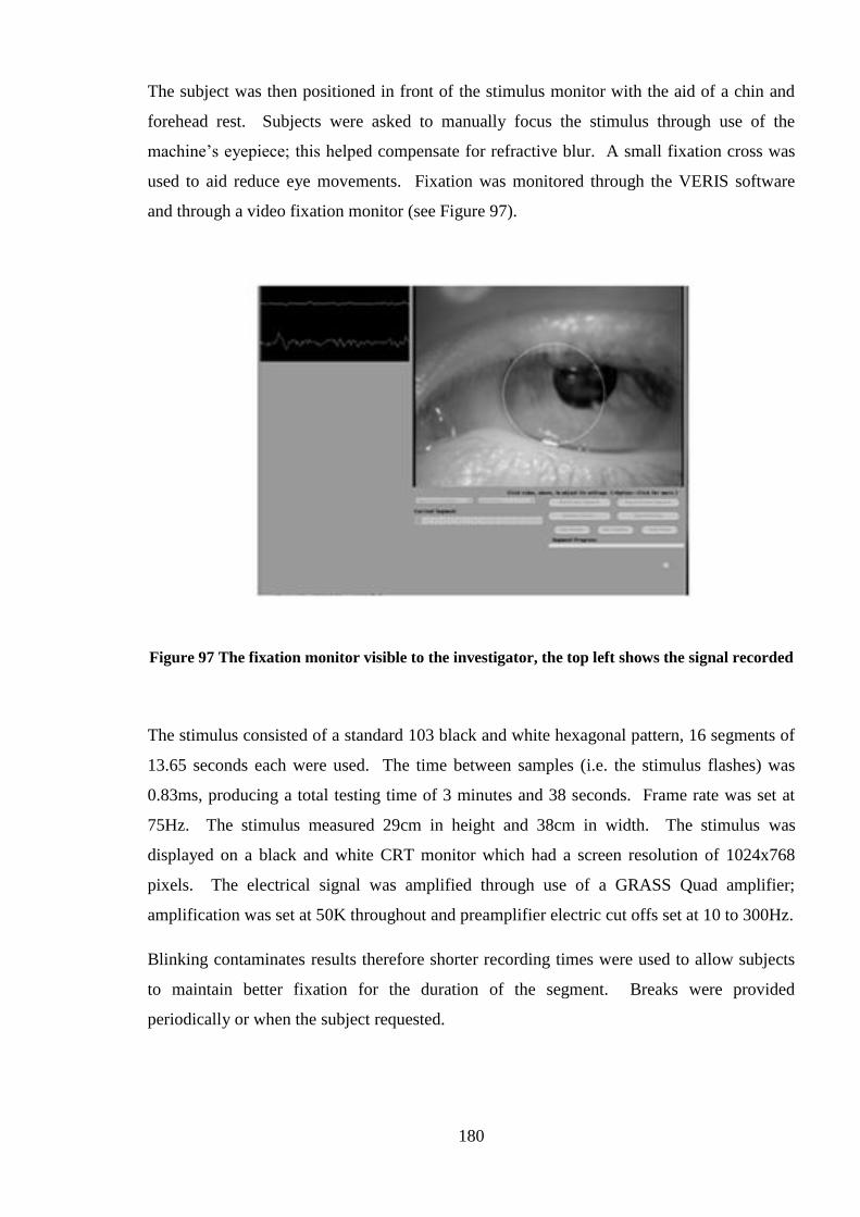
180

The subject was then positioned in front of the stimulus monitor with the aid of a chin and

forehead rest. Subjects were asked to manually focus the stimulus through use of the

machine‘s eyepiece; this helped compensate for refractive blur. A small fixation cross was

used to aid reduce eye movements. Fixation was monitored through the VERIS software

and through a video fixation monitor (see Figure 97).

Figure 97 The fixation monitor visible to the investigator, the top left shows the signal recorded

The stimulus consisted of a standard 103 black and white hexagonal pattern, 16 segments of

13.65 seconds each were used. The time between samples (i.e. the stimulus flashes) was

0.83ms, producing a total testing time of 3 minutes and 38 seconds. Frame rate was set at

75Hz. The stimulus measured 29cm in height and 38cm in width. The stimulus was

displayed on a black and white CRT monitor which had a screen resolution of 1024x768

pixels. The electrical signal was amplified through use of a GRASS Quad amplifier;

amplification was set at 50K throughout and preamplifier electric cut offs set at 10 to 300Hz.

Blinking contaminates results therefore shorter recording times were used to allow subjects

to maintain better fixation for the duration of the segment. Breaks were provided

periodically or when the subject requested.

181

Average N1 and P1 amplitudes and implicit times were examined by the standard concentric

ring formats and then again by quadrants (+Q and XQ, as previously defined in Chapter 9,

also see Figure 98).

Figure 98 The method by which mfERG rings and quadrants configurations were divided

before responses from each region were averaged and analysed

The N1 and P1 amplitudes and implicit times for the concentric ring averages were

investigated with reference to axial length and also refractive error. The N1 and P1

amplitudes and implicit times for the quadrant averages were investigated with reference to

axial length, refractive error and indices of shape derived from MR imaging.

Refractive error measurements were made using the Shin Nippon 5000 autorefractor;

measurements were made under cycloplegia. Axial length measurements were made using

the Zeiss IOL Master (see 7.2 and 7.3).

Twenty-one of the 23 subjects underwent MR scanning and from these data calculations of

IV were made for each quadrant; the CIs were then compared to each of the mfERG

responses (N1 amplitude, N1 implicit time, P1 amplitude, and P1 implicit time).

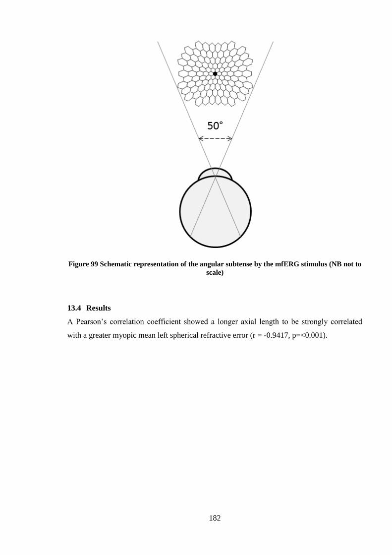
182

Figure 99 Schematic representation of the angular subtense by the mfERG stimulus (NB not to

scale)

13.4 Results

A Pearson‘s correlation coefficient showed a longer axial length to be strongly correlated

with a greater myopic mean left spherical refractive error (r = -0.9417, p=<0.001).

183

Figure 100 The PCI axial length against the mean spherical error (MSE) as measured by the

Shin Nippon autorefractor (n=23, left eye data)

Ring Configuration

The standard mfERG concentric ring configurations were analysed. Central refers to the

hexagon corresponding with the foveal response, and R5 corresponds to the peripheral

retinal response.

As expected the N1 and P1 amplitudes declined significantly with increasing retinal

eccentricity (p<0.01) in line with a decrease cell density (see Figure 101 and Figure 102).

Figure 101 N1 amplitudes shown as a function of retinal eccentricity (R5 indicates the ring

furthest from the fovea). Error bars show standard deviation of the dataset

y = -0.3711x + 23.518

R² = 0.8868

22.5

23

23.5

24

24.5

25

25.5

26

26.5

27

27.5

-10 -8 -6 -4 -2 0 2

Axia

l le

ng

th i

n (

mm

)

MSE (in D)

-60

-50

-40

-30

-20

-10

0

Centre R1 R2 R3 R4 R5

N1

AM

PL

ITU

DE

(in

nV

/deg

^2)

RETINAL REGION

184

Figure 102 P1 amplitudes shown as function of retinal eccentricity. Error bars show standard

deviation of the dataset

A Pearson‘s two tailed linear correlation coefficient was used to evaluate the effect of axial

length, and separately, refractive error on four components of the response waveform: N1

implicit times, N1 amplitudes, P1 implicit times, P1 amplitudes. Each of the four responses

were evaluated by the retinal region as defined by the rings; a Bonferroni correction was

used as there were six retinal regions in total, thus a critical p value of 0.05/6=0.0083 was

used. Results showed neither axial length nor refractive error correlated significantly with

each of the four responses for any of the six regions.

To investigate further potential differences between emmetropic and myopic mfERG

responses a 2-way mixed ANOVA was used to evaluate the responses from the four types of

response (i.e. N1 and P1 implicit times and amplitudes) for each of the six ring retinal

regions. The four responses did not show a significant difference between the two refractive

groups (p<0.05).

0.0

20.0

40.0

60.0

80.0

100.0

120.0

140.0

Centre R1 R2 R3 R4 R5

P1

AM

PL

ITU

DE

(in

nV

/deg

~^

2)

RETINAL REGION

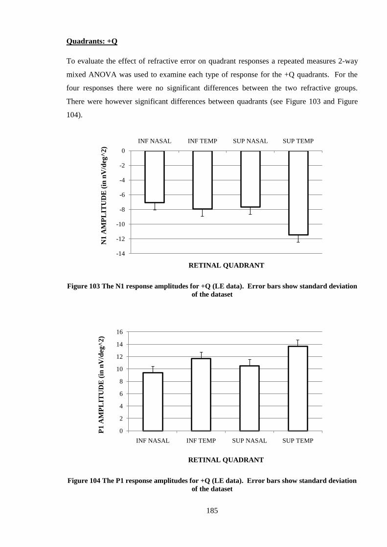
185

Quadrants: +Q

To evaluate the effect of refractive error on quadrant responses a repeated measures 2-way

mixed ANOVA was used to examine each type of response for the +Q quadrants. For the

four responses there were no significant differences between the two refractive groups.

There were however significant differences between quadrants (see Figure 103 and Figure

104).

Figure 103 The N1 response amplitudes for +Q (LE data). Error bars show standard deviation

of the dataset

Figure 104 The P1 response amplitudes for +Q (LE data). Error bars show standard deviation

of the dataset

-14

-12

-10

-8

-6

-4

-2

0

INF NASAL INF TEMP SUP NASAL SUP TEMP

N1 A

MP

LIT

UD

E (

in n

V/d

eg^

2)

RETINAL QUADRANT

0

2

4

6

8

10

12

14

16

INF NASAL INF TEMP SUP NASAL SUP TEMP

P1

AM

PL

ITU

DE

(in

nV

/deg

^2)

RETINAL QUADRANT

186

The N1 amplitudes showed significant differences across all quadrants (p<0.01) bar the

inferior-nasal vs. superior-nasal and also the inferior-temporal vs. superior-nasal. Significant

differences were noted across all P1 amplitude quadrant responses. The superior- temporal

quadrant showed the highest amplitude and the inferior-nasal quadrant was found to have the

lowest amplitude.

There were no significant differences between the implicit times of quadrants. Linear

correlations through use of Pearson‘s correlation coefficient showed that all four types of

mfERG response failed to correlate with refractive error or axial length.

The four types of response did not correlate with the IV for any quadrant. Surface areas

showed a significant correlation with N1 implicit times for the inferior-nasal quadrant only

(p=0.006, r= 0.583); all other combinations of +Q surface areas and mfERG responses failed

to show significant correlations (see Figure 105).

Figure 105 Surface areas and implicit times for the inferior-nasal retinal quadrant

y = 0.0186x + 10.002

R² = 0.3403

10

11

12

13

14

15

16

17

18

190 210 230 250 270 290 310 330

Inf-

Nasa

l im

pli

cit

tim

es (

ms)

Surface areas (mm²)

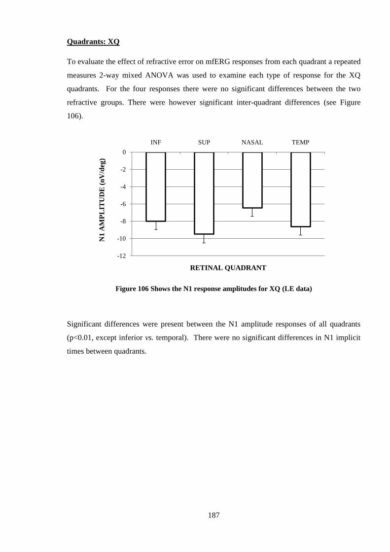
187

Quadrants: XQ

To evaluate the effect of refractive error on mfERG responses from each quadrant a repeated

measures 2-way mixed ANOVA was used to examine each type of response for the XQ

quadrants. For the four responses there were no significant differences between the two

refractive groups. There were however significant inter-quadrant differences (see Figure

106).

Figure 106 Shows the N1 response amplitudes for XQ (LE data)

Significant differences were present between the N1 amplitude responses of all quadrants

(p<0.01, except inferior vs. temporal). There were no significant differences in N1 implicit

times between quadrants.

-12

-10

-8

-6

-4

-2

0

INF SUP NASAL TEMP

N1 A

MP

LIT

UD

E (

nV

/deg

)

RETINAL QUADRANT

188

Figure 107 The P1 response amplitudes for the XQ (LE data). Error bars indicate the

standard deviation

There were significant differences noted between the P1 amplitude responses of all

quadrants (p<0.01) bar the inferior vs. temporal and superior vs. temporal (see Figure 107).

Figure 108 Shows P1 Implicit times for the XQ (LE data). Error bars indicate the standard

deviations

0

2

4

6

8

10

12

14

16

18

INF SUP NASAL TEMP

P1

AM

PL

ITU

DE

(n

V/d

eg)

RETINAL QUADRANT

27.5

28

28.5

29

29.5

30

30.5

31

31.5

INF SUP NASAL TEMP

P1 I

MP

LIC

IT T

IME

(IN

MS

)

RETINAL QUADRANT

189

There were significant differences between the P1 implicit times of all quadrants (p<0.05)

bar the inferior vs. temporal and superior vs. temporal (see Figure 108). Two tailed

Pearson‘s correlations for each of the four responses failed to show significant correlations

with refractive error, axial length, and IV. Surface areas and N1 implicit times for the

inferior quadrant were significantly correlated (p=0.004, r=0.599).

Figure 109 Surface areas and N1 implicit times for the inferior retinal quadrant

y = 0.0282x + 8.338

R² = 0.3593

10

11

12

13

14

15

16

17

18

200 220 240 260 280 300

N1 I

MP

LIC

IT T

IME

(m

s)

Surface areas (mm²)

190


The first negative (N1) and first positive (P1) components of the mfERG response waveform

were assessed; the response of these components originates mainly from the cone receptors

and bipolar cells. As expected the response amplitudes, for both N1 and P1, declined with

increasing retinal eccentricity. The decline with increasing eccentricity has been well

documented and is believed to relate to the concomitant decline in cone photoreceptors.

Inspection of standard deviations showed inter subject variability to be greatest in the foveal

region, this has also been noted previously (Nagatomo et al 1998). The variability in the

foveal region has often been attributed to the differences in the retinal cell topography

between individuals (Curcio et al. 1990).

In the current study refractive error did not correlate with mfERG responses to a significant

level for either ring or quadrant formats. Responses also failed to correlate with axial length.

Additionally, correlations with IV did not reveal significant relationships. There were two

correlations with surface areas; the implicit times of the N1 component correlated

significantly for the inferior and the inferior-nasal retina.

For this particular subject group it can be concluded that refractive error was not related to

mfERG responses. Specific aspects of ocular shape correlate with N1 implicit times for

some quadrants only. In general the relationship between ocular shape and mfERG

responses is weak.

Quadrant differences

A surprisingly few number of studies have examined the link between quadrant variations in

mfERG with refractive error. In the current study both +Q and XQ quadrants were

examined. Although refractive error did not correlate with quadrants, inter quadrant

differences were observed. The +Q quadrants showed significant differences in both the N1

and P1 amplitudes; highest amplitudes were noted in the superior-temporal retina and lowest

in the inferior-nasal retina. Reduced amplitudes with normal implicit times may indicate

damage to the cone photoreceptors (Hood et al. 2002).

For the XQ quadrants the nasal retina showed significantly reduced amplitudes and

significant delays in implicit time. This combination of responses indicates damage to the

cone receptors and the ON bipolar cells. If these responses are considered in the context of

retinal cell distribution then cone photoreceptor density is actually far greater in the nasal

191

retina than the temporal (Curcio et al. 1991), which is inconsistent with the results found.

However, the reduced nasal retinal response may be attributable to the optic nerve head

(ONH). In visual fields research the area represented by the ONH is removed from data

analysis. In the case of mfERG it can be difficult to isolate the hexagon representing the

optic nerve head and in some cases may not be possible at all. The reduced response in the

nasal quadrant may represent the ONH and although it would confirm that subjects were

properly fixating throughout the recording, an unfortunate consequence would be that direct

comparisons of quadrants would be rendered invalid.

In the current study highest amplitudes and shortest implicit times for the XQ quadrants were

noted in the superior retina. Similar findings have been reported in studies of hemifield

responses which have compared responses for the superior vs. inferior regions. The superior

retina is frequently reported to produce better responses than the inferior (Kawabata & chi-

Usami 1997)

Absence of a shape or refractive error effect on mfERG responses

Previous literature has reported on the reduction of mfERG responses in myopic subjects. It

is often the responses of progressing myopes or high myopes, not stable myopes, which are

found to be significantly different to emmetropes. In the current study all the myopes were

believed to be stable and only 5 of the 23 subjects exceeded levels of myopia which would

normally be classed as high myopia (i.e. greater than -6D MSE), therefore a reduced

response would not necessarily be expected. Furthermore the differences previously

reported in progressing or high myopes do not appear to display a clear or definite pattern of

reduced response. Examination of previous literature shows that no systematic variation

with refractive error has been reported. Previously it has been suggested that ocular shape

may be responsible for variations in mfERG response (Kawabata & chi-Usami 1997),

however the results from the present study are in disagreement with this view as the majority

of shape indices have not correlated with mfERG responses.

Unlike a number of previous studies of mfERG and myopia, spatial averaging was not

applied to the results. A strict criterion of rejecting noisy data was applied by experienced

electrophysiologists (Andrea Scott and Dr Ian Fawcett).

The current study would be extended through inclusion of subjects with progressive and high

myopia. Based on previous reports (Chen et al. 2006a) and the current study it is

192

hypothesised that the mfERG responses of progressive and high myopes will significantly

differ from that of emmetropes and stable myopes.

13.6 Summary

The mfERG response is known to vary greatly between individuals. Previous reports of

reduced mfERG responses in myopic subjects are not supported by the current study;

however, this may be due to the type and level of myopia tested. This study shows that

indices of ocular shape based on MRI data do not correlate well with mfERG responses,

except in the inferior and inferior-nasal quadrants. The evidence suggests that there is

limited support for a relationship between ocular shape and mfERG response. In general

stable myopic subjects retained mfERG response levels similar to those measured in

emmetropic subjects.

193

14 INVESTIGATION OF GANGLION CELL DENSITY WITH REFERENCE TO

OCULAR SHAPE

14.1 Introduction

Beyond the central foveal region the numbers of cone receptors rapidly decrease (Curcio et

al. 1990). The peripheral retinal regions are therefore poor at resolving detailed high spatial

resolution images. The ganglion and rod cells dominate these peripheral regions with a

minority number of cone cells.

The sampling theorem dictates that for a sinusoidal grating to be detected and reconstructed

accurately, two sampling points are required for each cycle of the waveform. The limit of

the sampling frequency is referred to as the Nyquist limit. If the drifting sinusoidal grating is

spatially undersampled, its direction of motion will reverse. In consequence, performance

will fall below 50% correct (e.g. See Figures 1-4 in Anderson et al. 1995).

Previous reports have suggested that the increase in ocular size, synonymous with myopia,

can lead to an increase in the distance between ganglion cells (Chui et al. 2004) which may

cause the resolution ability of the ganglion cells to be reduced (Thibos et al. 1987).

Conversely, predicted models of myopic eye shape correlated with calculations of ganglion

cell density have failed to explain reductions in peripheral visual acuity (Strang et al. 1998).

Until recently acquisition of accurate parameters of eye shape were limited to one

dimensional longitudinal measurements. The introduction of three dimensional ocular

Magnetic Resonance Imaging MRI (Singh et al. 2006) allows ocular shape to be investigated

in substantially more detail allowing direct associations to be made between ocular shape

and ocular function.

The methodology for measuring ganglion cells density in vivo, through psychophysical

methods has been well established (Thibos et al. 1987; Anderson et al. 1992; Anderson et al.

1995). The current study uses a modification of a protocol developed and reported by

Anderson et al. 1995 to investigate the relationship between ocular shape and ganglion cell

density (see Methods section). This study is the first attempt at correlating structural data

from ocular MRI with psychophysical estimates of ganglion cell density. The aim is to

construct a more informed report to determine whether eye shape affects retinal receptor

density or function.

194

14.2 Purpose

To evaluate the effects of myopic ocular expansion on ganglion cell density.

14.3 Hypothesis

The degree of myopia is significantly correlated with longitudinal axial length and eye size

(Singh et al. 2006). Previous work has shown ganglion cell density to be reduced in myopia

(Chui et al. 2004). It is hypothesised that subjects with myopic refractive errors and hence

relatively larger eyes will have poorer detection ability; as a consequence these subjects will

show an aliasing or distortion of the visual signal at lower spatial frequencies than

emmetropic subjects.

14.4 Methods

There are two main methods available to measure ganglion cell density in humans. The

most direct technique is through in vitro examination of retinal histological samples. In

contrast, in vivo ganglion cell sampling can be achieved through the use of psychophysical

techniques. The protocol used was adapted from a study by Anderson et al. (1995).

Four young adult female subjects (aged between 26-29 years) with good ocular health acted

as subjects. All subjects had previously undergone ocular MR scanning and a range of ocular

biometric measurements taken prior to the experiment. All volunteers were unpaid.

Informed consent was obtained from the four subjects.

Each of the four subjects (two emmetropes and two myopes) were tested monocularly

through natural pupils. The non-cycloplegic peripheral refractive error of the right (test) eye

as determined by retinoscopy at 40° eccentricity to the fovea in the temporal retina was

corrected by use of full aperture trial lenses (see Table 23). The contralateral eye was

occluded through use of an eye patch.

All subjects were postgraduate optometrists, accustomed to visually demanding tests for

research purposes and known to possess accurate fixation and concentration. Subjects were

seated so that the stimulus was in line with the primary direction of gaze. Fixation was well

controlled through vocal prompting and repeatedly checking subjects‘ eyes. Tests were

repeated a minimum of 25 times at each spatial frequency. Regular breaks were offered at

each spatial frequency change and taken by all subjects as required.

195

Figure 110 Diagram showing the experimental setup (not to scale)

The experiment was divided into two parts; sensitivity to (a) stimulus detection and (b)

stimulus direction discrimination.

Subject Refractive error, D Central error (MSE D) Peripheral error (D)

Subject OH -8.12/-1.00 x 85 -8.62D -5.00/-0.50 x 70

Subject MN -3.00DS -3.00 -2.12/-0.75 x 42

Subject AS +0.75/-0.50 x 180 +0.50 +0.50/-4.00 x 80

Subject JA +0.50/-0.62 x 118 +0.19 -3.00/-2.25 x 180

Table 23 Central and peripheral refractions (at ~40° temporal to fovea) of subjects corrected

with full trial aperture lenses (right eyes)

Subject

Axial length (mm)

(from MRI measurements for consistency with

ocular stretch index-see results)

Central corneal radii (mm)

(from the Zeiss IOL Master)

Subject OH 25.96 7.62/7.5

Subject MN 25.67 7.89/7.84

Subject AS 23.78 8.06/7.87

Subject JA 23.68 8.06/7.98

Table 24 Biometric data of subjects

196

Axial lengths were consistent with the well established relationship between a longer axial

length and higher degrees of myopia.


In order to exploit the on/off centre arrangement of the ganglion cells a sinusoidal grating

stimulus was presented on a 21 inch Sony GDM-F520 Trinitron CRT monitor with 100Hz

frame rate, in a dimly lit room. Screen resolution was 1024 x 768 pixels. Stimulus size was

approximately 9.7cm wide and 9.5cm in height. Subjects had a viewing distance of 1m. The

edges of the stimulus were blurred to limit edge detection and accommodative responses, by

use of translucent paper. A fixation target was located 84cm from the stimulus, at a viewing

angle of 40° relative to the primary line of sight.

Peripheral refractions at 40° eccentricity of the temporal retina were carried out using a

Keeler streak retinoscope by an experienced practitioner, and refractive errors corrected

using full aperture lenses to limit refractive blur. Lenses were secured by use of a standard

Oculus trial frame, at a back vertex distance of approximately 11mm.

14.5.1 Stimulus detection

A two alternative forced choice experimental protocol was employed, through use of a

subject controlled keypad. The experiment was commenced, and could be paused, by the

subject‘s keypad.

Twenty five pairs of stimulus intervals were shown on the screen; each pair presented either

a horizontal sinusoidal grating or a blank screen. Subjects were asked to indicate in which of

the two randomly ordered presentations the stimulus was present.

Subjects repeated this procedure a minimum of 25 times for each spatial frequency. Spatial

frequencies ranged from 1 to 7 c/deg (cycles per degree) in steps of 1 c/deg, or 0.5 c/deg

when required. After 25 runs at a given spatial frequency the computer program produced a

score expressed as a percentage of correct responses. The upper limit of spatial frequencies

was largely dependent on the point at which a subject was unable to achieve a score above

50%. Responses at 50% were assumed to be the point at which aliasing took place. A

Michelson contrast of 80% for the sinusoidal stimulus was maintained throughout by use of

197

the computer program settings. Subjects were encouraged to take regular breaks to minimise

the influence of fatigue between recordings of each spatial frequency.

14.5.2 Stimulus direction discrimination

The same protocol was used as that for detection with the exception of the blank screen i.e. a

stimulus was shown in both presentations. The stimulus grating moved in either an upwards

or downwards direction. Subjects were asked to identify in which presentation, the first or

second, the grating appeared to be moving upwards.

14.5.3 Validity

The validity of the technique is well established. Psychophysical techniques have proven to

be sensitive and valid predictors of ganglion cell density through comparisons to histological

data (Anderson et al. 1992; Curcio et al 1990). The protocol used in the current study

matches that of a similar experiment by Anderson et al.1995. The computer program for the

above procedure was written and developed by Professor SJ Anderson, Aston University.

14.6 Results

Right eye results for discrimination and detection experiments:

14.6.1 Detection and direction discrimination experiments

As expected all subjects demonstrated a decline in stimulus detection as spatial frequency

increased.

AVERAGE OF % CORRECT

Spatial Frequency (c/deg) Subject OH Subject MN

1

98±2.83 100

2

100 96

3

86.67±10.07 88

4

76±26.23 81.33±14.05

5

69.33±8.33 84±5.66

6

45.33±10.07 52

7

48

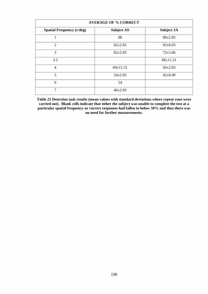
198


Spatial Frequency (c/deg) Subject AS Subject JA

1

88 98±2.83

2

82±2.83 92±6.93

3

82±2.83 72±5.66

3.5

68±11.31

4

60±11.31 50±2.83

5

54±2.83 42±8.49

6

54

7

46±2.83

Table 25 Detection task results (mean values with standard deviations where repeat runs were

carried out). Blank cells indicate that either the subject was unable to complete the test at a

particular spatial frequency or correct responses had fallen to below 50% and thus there was

no need for further measurements.

199

Figure 111 Subject OH, MSE: -8.62D. Vertical lines express 95% confidence limits, solid lines

show confidence limits for the detection function and dashed line for the direction

discrimination

Subject OH

Subject OH was the most myopic of the 4 subjects. Detection ability fell to below chance

between 5-6 c/deg. Direction discrimination fell to below chance (correct responses ≤50%)

at 5-6 c/deg also.

0

10

20

30

40

50

60

70

80

90

100

0 1 2 3 4 5 6 7

Per

cen

tag

e o

f co

rrec

t re

spo

nse

s (%

)

Spatial frequency (cycles per degree)

Detection Direction discrimination

200

Figure 112 Subject MN, MSE: -3.00D

Subject MN

Subject MN showed detection performance to fall below chance at 6-7 c/deg. Direction

discrimination fell below chance at 6-7 c/deg. Subject MN‘s results showed motion reversal

at 6 c/deg.

0

10

20

30

40

50

60

70

80

90

100

0 1 2 3 4 5 6 7

Per

cen

tag

e o

f co

rrec

t re

spo

nse

s (%

)



201

Figure 113 Subject AS, MSE: +0.50D

Subject AS

Subject AS showed detection ability to decline to below chance at 6-7 c/deg; direction

discrimination fell to below chance at 3 c/deg. Subject AS also displayed motion reversal

(evidence of aliasing); this was noted at 5 c/deg.

0

10

20

30

40

50

60

70

80

90

100

0 1 2 3 4 5 6 7

Per

cen

tag

e o

f co

rrec

t re

spo

nse

s (%

)



202

Figure 114 Subject JA, MSE: +0.19D

Subject JA

Detection ability fell below chance at only 4 c/deg; the lowest of the four subjects. Direction

discrimination ability fell below chance at 3 c/deg. Subject JA also displayed motion

reversal at 5 c/deg.

0

10

20

30

40

50

60

70

80

90

100

0 1 2 3 4 5 6 7

Per

cen

tag

e o

f co

rrec

t re

spo

nse

s (%

)



203


Spatial Frequency Subject OH Subject MN

1 100 100

2 98±2.83 96

3 70±2.83 64

3.5 68 52

4 56±11.31 57.33±6.11

5 48 56

6

48


Spatial Frequency Subject AS Subject JA

1 98.67 64.33±5.66

2 72 58±8.49

2.5

50.17±2.83

3 50 41±5.66

3.5 46

4 54.67 26.67±2.83

5

39

Table 26 Direction discrimination task results (mean values with standard deviations where

repeat runs were carried out)

All subjects bar subject OH (the most myopic subject) showed motion reversal, which is

clear evidence of signal aliasing. In many of the experiments (75%) the Nyquist limit fell

between two spatial frequencies. Linear interpolation was used to gauge a more accurate

estimate of the Nyquist limit. All subjects bar Subject MN showed the direction

discrimination threshold to be lower than the detection threshold. The difference for Subject

MN was minimal (0.3 c/deg).

14.6.2 The effect of eye conformation on ganglion cell receptors

To study the relationship between eye shape on the two experimental protocols detection and

direction discrimination, previously acquired ocular MR scans for each subject were

analysed. In order to quantify retinal stretch, a ratio for the index of stretch was calculated;

additionally surface area for the temporal retinal quadrant strip which lay 60-80% along the

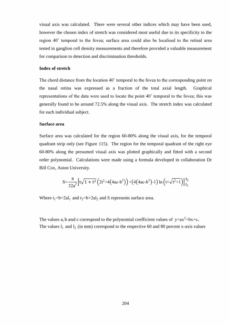
204

visual axis was calculated. There were several other indices which may have been used,

however the chosen index of stretch was considered most useful due to its specificity to the

region 40˚ temporal to the fovea; surface area could also be localised to the retinal area

tested in ganglion cell density measurements and therefore provided a valuable measurement

for comparison to detection and discrimination thresholds.

Index of stretch

The chord distance from the location 40˚ temporal to the fovea to the corresponding point on

the nasal retina was expressed as a fraction of the total axial length. Graphical

representations of the data were used to locate the point 40˚ temporal to the fovea; this was

generally found to be around 72.5% along the visual axis. The stretch index was calculated

for each individual subject.

Surface area

Surface area was calculated for the region 60-80% along the visual axis, for the temporal

quadrant strip only (see Figure 115). The region for the temporal quadrant of the right eye

60-80% along the presumed visual axis was plotted graphically and fitted with a second

order polynomial. Calculations were made using a formula developed in collaboration Dr

Bill Cox, Aston University.

S=

32a2 2t2 4 4ac b2 4 4ac b2 1 ln t t2 1

t2t1

Where t1=b 2al1 and t2=b 2al2 and S represents surface area.

The values correspond to the polynomial coefficient values of y=ax2 bx c. The values l1 and l2 (in mm) correspond to the respective 60 and 80 percent x-axis values

205

Figure 115 Diagrammatical representation of the surface area calculation of the ocular surface.

The grey band represents the 60-80% region for which area was calculated (not to scale)

Subject Detection NL Direction

Discrimination NL

Index of stretch

(%)

Surface area

(mm²)

Subject O.H 6.8 4.8 93 112.95

Subject M.N 6.5 6.8 91 97.82

Subject A.S 6.5 3 99 95.02

Subject J.A 4 2.5 92 85.03

Table 27 Calculated index of ocular stretch and Nyquist limit (NL) estimates calculated for

each subject (in %). NB a higher % for index of stretch indicates a smaller eye

206

Figure 116 Graphical representation of the spatial frequencies at which 50% of responses are

correct, plotted as a function of stretch index. Circles denote detection and stars indicate

direction discrimination. Case study RC is also included (see below).

From the four subjects in the main study myopic subjects OH and MN had the highest index

of stretch. The index of stretch was correlated with the threshold values for each subject in

each of the experiments. The estimate of the spatial frequency at which correct subject

responses were at the 50% level is shown in the table above. The ocular stretch did not

correlate with either detection threshold or direction discrimination threshold. Surface area

was calculated and shown to be larger in the myopic subjects OH and MN, however,

variation in surface area had no systematic effect on either detection or discrimination tasks.

It can be seen from the calculated indices of ocular stretch that there is much variation

between individual eye shape and variations may not occur as a function of refractive error.

Subject O.H

Subject M.N

Subject A.S

Subject J.A

Subject O.H

Subject A.S

Subject J.A

Subject R.C (RE)

Subject R.C (LE)

70

75

80

85

90

95

100

105

0 1 2 3 4 5 6 7 8

Ind

ex o

f st

retc

h i

n %

Limit in cycles per degrees

207

Figure 117 Calculated index of stretch for subject OH: 93%. The graph shows the point

situated 40° from the presumed foveal location; the horizontal lines denote the distance from

the 40° location to the presumed visual axis (RE) Negative values denote the temporal region

and positive numbers denote the nasal.

0

5

10

15

20

25

30

-15 -10 -5 0 5 10 15

Dis

tan

ce a

lon

g t

he

axis

(m

m)

Distance from the axis (mm)

Subject OH

208

Figure 118 Calculated index of stretch for subject MN: 91% (RE). Negative values denote the

temporal region and positive numbers denote the nasal

0

5

10

15

20

25

30

-15 -10 -5 0 5 10 15

Dis

tan

ce a

lon

g t

he

axis

(in

mm

)


Subject MN

209

Figure 119 Calculated index of stretch for subject AS: 99% (RE). Negative values denote the


0

5

10

15

20

25

30

-15 -10 -5 0 5 10 15

Dis

tan

ce a

lon

g t

he

axis

(in

mm

)


Subject AS

210

Figure 120 Calculated index of stretch for subject JA: 92% (RE). Negative values denote the


14.7 Case study

The four subjects above did not show a significant relationship between ganglion cell density

and the calculated ocular index of stretch. For a more robust comparison of the effect of

myopia a case study of a highly anisomyopic subject was carried out. The high level of

anisomyopia allowed the less myopic eye to act as a control.

Case study subject RC, a 45 year old male anisomyope underwent the same experimental

protocols for detection and direction discrimination, however both right and left temporal

retinae were tested.

Eye Central MSE

(D)

Refractive error at ~

40˚ temporal to fovea

(D)

Axial length

(from MRI, in

mm)

Corneal curvature

(from Zeiss IOL

Master, in mm)

Right -19.76 -8.00/-2.50 x 90 27.87 7.32/7.29

Left -2.75 -3.50/-1.50 x 90 21.93 7.38/ 7.12

Table 28 Refractive and ocular biometric data for subject R.C

0

5

10

15

20

25

30

-15 -10 -5 0 5 10 15

Dis

tan

ce a

lon

g t

he

axis

(m

m)


Subject JA

211

Results showed that an increase in spatial frequency led to a reduction in detection ability.

Detection ability was retained at a similar level in both the highly myopic right and the less

myopic (control) left eye, detection ability was still retained above 50% with stimuli of 6

c/deg. Direction discrimination fell below chance between 1.5-2 c/deg in both eyes. Linear

interpolation showed a reduction in direction discrimination ability for both eyes at 1.9

c/deg, despite a large difference in ocular stretch and surface area.

Figure 121 Case study: RC right eye

0

10

20

30

40

50

60

70

80

90

100

0 1 2 3 4 5 6 7

Per

cen

tag

e o

f co

rrec

t re

spo

nse

s (%

)



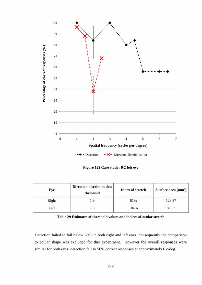
212

Figure 122 Case study: RC left eye

Eye Direction discrimination

threshold Index of stretch Surface area (mm²)

Right 1.9 81% 123.37

Left 1.8 104% 83.33

Table 29 Estimates of threshold values and indices of ocular stretch

Detection failed to fall below 50% in both right and left eyes, consequently the comparison

to ocular shape was excluded for this experiment. However the overall responses were

similar for both eyes; detection fell to 56% correct responses at approximately 6 c/deg.

0

10

20

30

40

50

60

70

80

90

100

0 1 2 3 4 5 6 7

Per

cen

tag

e o

f co

rrec

t re

spo

nse

s (%

)



213

Figure 123 Calculated index of stretch, subject RC, left eye: 104%. Negative values denote the


0

5

10

15

20

25

30

-15 -10 -5 0 5 10 15

Dis

tan

ce a

lon

g t

he

axis

(in

mm

)

Distance from the axis (in mm)

Subject RC

214

Figure 124 Calculated index of stretch, subject RC, right eye: 81%. Negative values denote the


14.7.1 Discussion and conclusions

The relationship between estimated ganglion cell density and stimulus detection has been

well documented: if the spacing of the ganglion cells is too large then the visual stimulus

will be undersampled, consequently aliasing (or misinterpretation) of the stimulus will occur

(Thibos et al. 1987). In myopic subjects reduced ganglion cell density has been reported

(Chui et al. 2004). This has been attributed to ocular expansion and subsequent retinal

stretch, both synonymous with high myopia. The numbers of psychophysical studies

reporting ganglion cell density in different refractive groups are limited. Current knowledge

is also limited by the little knowledge of ganglion cell density data through histological

analysis of eyes from a range of refractive groups.

The aim of the current investigation was to evaluate the effect of eye conformation on

ganglion cell density. Based on previous literature, an adverse effect i.e. increased ganglion

cell spacing was predicted in larger eyes (Chui et al. 2004; Vera-Diaz et al. 2005). Although

a previous attempt at correlating myopic stretch with ganglion cell density and visual acuity

0

5

10

15

20

25

30

-20 -15 -10 -5 0 5 10 15

Dis

tan

ce a

lon

g t

he

axis

(in

mm

)

Distance from the axis (in mm)

Subject RC

215

has been made, the study was based on theoretical assumptions of ganglion cell density and

models of myopic growth (Strang et al. 1998). In the present study the ocular shape was

determined through MR imaging, by a recently introduced technique which enables accurate

depictions of the 3D conformations of myopic eyes. Indices of retinal stretch and retinal

surface area were calculated based on the MR data; these parameters were subsequently

compared to the Nyquist limits for each individual subject. In the case of the highly

anisomyopic subject RC, a difference of approximately 22% in the index of stretch and 32%

in surface area was noted between the right and left temporal retinae. Consequently, the

direction discrimination of the right eye would be expected to lie in the range of 1.2-1.4c/deg

(based on the left eye threshold of 1.8c/deg), however, the right eye showed a direction

discrimination threshold of 1.9c/deg. Ganglion cell density failed to vary as a function of

both ocular stretch and surface area. The results would indicate that any decreases in

estimated ganglion cell density noted previously in the peripheral myopic retina are

independent of ocular shape.

14.7.2 Possible causes for the absence of a relationship between ganglion cell density

and ocular shape

Previous studies have reported reduced peripheral visual function or reduced ganglion cell

density as a consequence of ocular expansion; however these studies have investigated

much smaller eccentricities of 15˚ (Vera-Diaz et al. 2005) and 0, 5˚ and 15˚ (Chui et al.

2004) from the fovea. Others have constructed theoretical models of myopic eye shape and

attempted to correlate these with calculated values of ganglion cell density. The current

study is unique as an accurate depiction of the retinal shape in the region tested has been

obtained through MR imaging. The findings have been correlated for psychophysical

estimates of ganglion cell density at 40˚ eccentricity; this was the location at which

Anderson et al. (1995) carried out their study as preliminary trials had shown it to be an

optimal location for demonstrating motion reversal. Furthermore this point is approximately

coincident with the retinal area reported to show significant changes in retinal shape as a

function of refractive error (Gilmartin et al. 2007). The absence of a decline in response

with increasing myopia suggests that ganglion cell density is not reduced as a function of

shape. The findings cannot establish whether myopia and ganglion cell function are

independent factors.

216

The mechanical stretching of the retina is complex, furthermore the effect of ocular

expansion on retinal cells is difficult to ascertain. The ocular expansion in myopic eyes has

been presumed to affect retinal cells by increasing spacing between cells; this was not shown

in the current study. The view that stretching a tissue would lead to its components, the cells,

separating may be an overly simplistic view. It may be possible that if ocular stretch is

taking place perhaps the cells themselves also stretch, either as a consequence or part of the

myopic development process. This would imply that the ganglion cell receptive field

becomes larger allowing images of low spatial frequency to be detected, but would not

explain detection of high spatial frequencies. Damage to cells in individuals may also be

explained through cell stretch.

Secondly the impact of mechanical stress on each individual retinal layer in myopic growth

is unclear (Wolsley et al. 2008). Estimates of the magnitude of impact may be inferred from

measurements of retinal thickness. Retinal thickness measured by optical coherence

tomography (OCT) have shown the perifoveal regions in myopic subjects to be significantly

thinner particularly in the temporal retina (Coletta et al. 2008) and the central foveal region

to be thicker (Lam et al. 2007). Retinal thinning occurs most notably in the choroid located

in the outer segment next to the pigment epithelium (Ilkuno & Tano 2009).

Often the reasons cited for reduced functional response in myopia relate to the decreased

retinal cell density or retinal cell damage (Jaworski et al. 2006; Chen et al. 2006; Atchison et

al. 2006). Cell damage or misalignment is particularly relevant in the outer retina where

photoreceptors are direction specific and misalignment may lead to cessation of function

(Stiles & Crawford, 1934). To explain the lack of impact of ocular expansion on the

ganglion cell layer it is speculated that outer retinal layers may not be able to withstand

mechanical pressure as well as the inner retinal layers. The effect of stretch is likely to be

dependent on mechanical characteristics such as tensile strength and thickness of each

individual retinal layer (Wolsley et al. 2008).

Histological studies calculating the density of ganglion cells in retinal tissue samples for a

range of refractive errors would provide further insight into the effect of ocular expansion on

ganglion cells. Mechanical stress caused by myopia could be further explored by

measurement of individual retinal layer thickness, which would help demonstrate the impact

of myopic stretch on each retinal layer.

For the index of stretch considered and for retinal surface areas, ganglion cell density does

not correlate significantly. The finding is highlighted in the case of a highly anisometropic

217

subject. The results are contrary to previous findings of ganglion cell density with reference

to refractive error (Chui et al. 2004). It is hypothesised that individual retinal layers are

affected separately by the mechanical stress of myopic growth or in a way not yet

established. Ganglion cell density information through histological and retinal thickness

studies would help explain these results further.

14.8 Summary

In the two experimental protocols, detection and direction discrimination the level of ocular

expansion was unrelated to the point at which aliasing occurred. Owing to individual

variation in ganglion cell density, the comparison between emmetropic and isomyopic

thresholds are of limited value and therefore the case study of a highly anisomyopic subject

RC has been described.

Despite a large difference in the refractive error and index of expansion between the two

eyes, the Nyquist limit values for subject RC were similar for both eyes. The results suggest

that ganglion cell density does not reduce as a function of ocular stretch in myopia.

Histological analysis of individual retinal layers in eyes from a range of refractive errors

would provide further insight into the mechanical effects of myopia on retinal cells.

218

15 GENERAL DISCUSSION

15.1 Introduction

The principle aim of this thesis was to evaluate the relationship between ocular shape and

visual function. Previous works have identified both structural and sensory factors as

potential precipitants of myopic development. It was envisaged that this thesis could help

characterise the structural effects of myopia and subsequently facilitate the development of

future therapies for myopia prevention. In this thesis a unique application of a recently

introduced MR ocular imaging technique has been used to investigate ocular shape. The

evaluation of visual function has been made through several vehicles, enabling multiple

strata of the retina to be examined.

The thesis assesses direct comparisons of a popularly used technique to derive retinal

contour, peripheral refraction, with 3-dimensional MR imaging. The thesis reports on

previously unidentified structural variations in eye shape, some of which are independent of

refractive error and others which are not. Specifically quadrant variations in eye shape have

been described in detail. Furthermore, previously unknown variations in visual function

have been identified; the functional ability of the eye has been further explored with

reference to refractive error and eye shape.

The findings are of direct clinical relevance to optometrists and the evaluations of visual

function can contribute significantly to the management of the myopic eye. The findings

from the experimental work have the potential to lead to further research initiatives and

larger scale studies (see 15.4).

15.2 Eye shape and its role in myopia

In the 1970s a series of well known studies attributed the development of myopia in adults to

a relatively hyperopic peripheral image shell in comparison to the central refraction (Rempt

et al. 1971). The principal technique used to investigate this theory was peripheral

refraction. Peripheral refraction is not directly indicative of ocular shape; peripheral

refraction data require transformation before ocular shape may be inferred. Previously,

transformation of peripheral refraction data has shown myopic eyes to be relatively prolate,

or less oblate than their emmetropic counterparts. The ocular shape findings from peripheral

refraction data have been supported by measurements taken through ocular MR imaging

219

(Atchison et al. 2004; 2005). Until recently a significant proportion of the eye has remained

inaccessible to measurements; the advent of 3D MRI has allowed greater access to the eye in

vivo.

The results from the 3D MRI have shown multiple variations in eye shape some of which are

present irrespective of refractive error magnitude and others which are highly dependent on

refractive error. The variations which are independent of refractive state may be attributed

to natural or biological variations present in most subjects. Although these variations do not

necessarily help explain myopia, they do help in the understanding of ocular growth in

general.

Variations dependent on refractive state are most evident in the general size of the eye; eye

size increases as a function of increasing myopia. In all eyes there is a more spherical region

in the mid section of the eye (which begins approximately 40% along the optic axis);

although quadrant shape variations also exist. The irregularities noted within this apparently

spherical region led to the conclusion that a more irregular eye shape is present in the eyes of

both low myopic and emmetropic subjects in comparison to high myopes. The greater shape

regularity in the high myopic group could be attributed to ocular stretch.

Of particular note was the exaggerated growth of the temporal quadrant in myopia as

indexed by calculations of the maximum distances from the retinal surface to the presumed

visual axis. Although the temporal quadrant differences failed to reach statistical

significance they are still of interest as the temporal and superior quadrants are frequently

cited as the locations most affected by myopic degenerations which can in part be explained

by the tissue stress caused by the rapid myopic growth in these regions. The rationale for

why myopic changes manifest themselves in the temporal quadrant is unclear. Asymmetric

growth could be stimulated by several factors; asymmetric sensory input into the eye (e.g.

through ocular aberrations or extent of the visual field), structural factors (e.g. ocular muscle

action), or innate retinal tissue vulnerabilities which predispose specific quadrants to growth

in myopia.

A distinctive feature of this thesis is the comparison made between the two major techniques

of ocular imaging; MRI and transformed peripheral refraction data. The results showed that

retinal curvature readings obtained using the ocular 3D MRI were consistently flatter than

those using peripheral refraction. It was suggested that although a general correction factor

could be applied to the data in order to make the two techniques more comparable, the

presence of refractive group variations would compromise the accuracy of the correction

220

factor. It can be concluded that although peripheral refraction and MRI techniques produce

similar conclusions of eye shape measurements, the two techniques are not comparable.

In summary, some parameters of ocular shape are specifically variants of refractive error

(e.g. posterior ocular volume, posterior radius bands); other variations are unrelated to

refractive error (e.g. anterior volume, specific intra quadrant differences). The asymmetries

unrelated to refractive error could stem from the extra ocular muscles insertions, sensory

factors or anthropologic reasons.

15.3 Visual Function and ocular shape

Visual functionality of the human eye is affected by many factors. In addition to refractive

error, factors such as accommodative state, aberrations, visual experience, binocular status

and ocular pathology may all affect visual information received by the retinal receptors. It

has been suggested that sensory visual experience can mediate ocular growth and

development of refractive error; in this study several tests of visual functionality were

correlated with specific indices of ocular shape. The responses for each of the tests

originated from different layers of the retina. The purpose of this type of design was two-

fold; firstly by examining the function vs. shape relationship it can be elicited whether or not

ocular shape does affect functionality and indeed if special considerations or correction

factors should be taken into consideration when examining myopic eyes in a clinical

situation. Secondly, by using tests examining specific retinal layers the study was able to

draw out which retinal layers may be most affected by myopic stretch.

Figure 125 Schematic illustration of the retinal layers of the human eye

221

Visual field sensitivity is representative of the cone receptor response which originates from

the outer retina. The responses showed the superior and superior-temporal quadrants to be

correlated with eye shape. The inferior retinal quadrant response was significantly reduced

relative to the superior, nasal and temporal quadrants.

The responses from the mfERG originate largely from the bipolar cells and responses

correlated with shape indices in only the inferior and inferior-nasal quadrants. Highest

amplitudes were noted in the superior-temporal retina and lowest in the inferior-nasal retina.

The nasal retina showed significantly reduced amplitudes and significant delays in implicit

time.

In general, tests of visual function showed the superior retina to perform better than the

inferior; this was true of both mfERG and visual field tests. The nasal –temporal

asymmetries showed less consistency between mfERG and visual fields testing. Chord

distances from the MRI data showed the superior chords to be smaller than the inferior. If

chord distance is used as a representative of ocular stretch it can be theorised that increased

stretch may create a reduced functional response. For the MR indices which were correlated

with functional test results (i.e. surface areas and interval variance) there were very few

significant correlations.

Surface area in the visual fields and mfERG groups showed superior vs. inferior asymmetry:

the inferior surface area was larger than the superior. This would indicate that the inferior

quadrant is further from the presumed visual axis and has a larger surface area i.e. it is

enlarged. From these results we may form the hypothesis that the retinal receptors are further

stretched and subsequently produce reduced functional response in the inferior retina.

The ganglion cell density was tested through psychophysical methods. It was expected that

the ganglion cell density would decline as a function of increasing myopia. Of particular

interest was a case study examining the eyes of a highly anisomyopic individual; the results

showed little difference in the responses of the two eyes. The results led to the conclusion

that despite a large refractive difference and a large difference in eye shape the ganglion cell

density was retained at similar levels.

222

15.4 Further work

15.4.1 Orbital size versus ocular size

All aspects of the experimental work allow scope for further development of the subject

area. With reference to ocular shape, there have been theories presented proposing that the

exaggerated axial growth in myopia is due to minimal restriction to longitudinal growth by

the posterior aspect of the globe. Vertical and horizontal restrictions to growth are imposed

by the orbital walls. This theory has thus far only been explored, and subsequently

disproved, in the eyes of Far Eastern subjects (Chau et al. 2004), who are well known to

have different shaped eyes to White-Caucasian subjects (Logan et al. 2004). As part of the

MRI experimental work in this thesis an attempt was made to compare orbital and ocular

size, however, the resolution of the images was not sufficient to allow accurate

measurements. Recently, the introduction of 7-tesla MRI has allowed high resolution

images to be obtained (Richdale et al. 2009). Examination of subjects who have undergone

this type of scanning may help explore this theory further.

15.4.2 Advanced data analysis and development of myopia treatments

The use of more advanced analysis techniques on the current data set is required. In

particular more recent research advocates the use of finite element analysis for analysing

biological tissues. In order to quantify the impact of myopic stretch and growth, the

emmetropic eye may be used as a reference, or undeformed state, and the myopic eye as a

state of deformation. Using this approach the quantification of changes may allow more

accurate preventative treatments for myopia to be developed. The findings may also be used

in conjunction with peripheral refraction findings. Currently, peripheral refraction data is

being used to develop contact lens treatments to inhibit myopic development.

15.4.3 Extending peripheral refraction work

Although not detailed in the main body of this thesis, a case study was carried out on a

highly myopic subject, whereby peripheral refractive measures were obtained under a

cycloplegic state and then with contact lenses in situ (see appendices, Figure 132). The case

study demonstrated the significant amount of peripheral hyperopic defocus; leading to the

conclusion that contact lens wear may in fact stimulate myopic growth. A study calculating

223

the image shells of subjects with and without their contact lenses in situ may help quantify

the level of peripheral hyperopic defocus and perhaps identify which contact lens design is

most suitable for use in myopes.

The development of a peripheral refractive device for measurement of multiple meridians

would greatly aid the development of more accurate contact lens designs in the prevention of

myopia.

A further aspect of the peripheral refraction dataset could be examined to determine whether

or not a ‗mirror-effect‘ exists between the right and left eyes, i.e. the temporal readings of

the left and right eyes are similar, and the nasal readings of the left and right eyes are similar.

Previously a mirror-effect has been noted through peripheral refraction measurements

(Seidemann et al. 2002). Interestingly the current cohort showed inter eye differences in eye

shape as determined by MR imaging, it would be interesting to quantify the inter eye

discrepancies between the two techniques.

15.4.4 Identifying high risk cases of myopia

One key finding has been the excessive growth of the temporal quadrant in myopia.

Although the finding did not reach statistical significance it is still particularly interesting as

the temporal retina has frequently been identified as a site of myopic degeneration. A larger

cohort study in combination with a longitudinal study of myopic fundus changes would help

identify at which level of myopia significant fundus changes occur, whether the changes in

ocular shape precede the visible fundus changes, and perhaps most importantly, at which

level of myopic refractive error is the risk of developing a visible fundus change increased.

A visible myopic degeneration is highly correlated with the development of retinal

detachments which can lead to ocular morbidity. The findings could be used to review the

current criteria for NHS eye tests for myopic patients and also the frequency at which

patients are reviewed.

15.4.5 Anterior eye biometric and functional investigations

A further interesting finding of this thesis was concerning the structural characteristics of the

anterior eye. The findings from the MRI and Oculus Pentacam data showed a spectrum of

changes in the anterior eye; for some parameters such as ocular volume the anterior eye

measurements remain homogenous across all refractive error groups, but for other measures

224

such as chord differences and pachymetry there are notably asymmetries between quadrants.

As yet it is unclear whether the anterior eye plays a homeostatic regulatory role in preventing

myopia or is in fact a contributor to myopic development. The cornea itself is known to

possess homeostatic qualities in the regulation of epithelial cells, noted in studies examining

post surgery wound healing (Wilson et al. 2003). Further analysis of both the current data

set and additional anterior eye biometric measures will help further characterise the role of

the anterior eye.

15.4.6 Histological studies

The functional aspect of the project has drawn interesting conclusions revealing the presence

of multiple variations in the retinal responses of the different retinal quadrants. In general,

highly myopic eyes are expected to show increased cell spacing and thus reduced visual

function, however, the results from this thesis have not substantiated these claims. Many of

the functional changes were present irrespective of refractive error and eye shape.

The findings from this thesis provide a basis for further research, in particular histological

studies which examine the retinal receptor cell spacing in cohorts with a range of ametropia.

Additionally histological studies of the anterior eye, namely the cornea may be beneficial in

identifying the corneal layer most affected in ametropia through both cell density and

thickness.

15.5 Summary

In conclusion, this investigation of ocular shape has described a variety of previously

unknown variations in eye shape, some of which are present irrespective of refractive error.

The structural changes which occur as a consequence of myopia have been noted and

discussed. The posterior eye appears most affected by myopia although it is unclear whether

the changes are a consequence or precipitant of myopia. The potential role of the anterior

eye has been discussed and briefly investigated. Many parameters remain unchanged in the

myopic anterior eyes, others act contrary to hypotheses. It is unclear whether the anterior

eye plays either a regulatory role in myopic development or is a contributory factor itself.

The question of why homeostatic regulations fail remains unanswered, although genetic

structural vulnerabilities could play a role in addition to environmental sensory stresses such

as near work.

225

The study provides scope for further investigations, including further analysis of the existing

dataset. It is envisaged that engineering methodologies such as finite element analysis will

enable the construction of more accurate myopic models of eye shape which may be used in

the development of myopic preventative therapies namely in the form of contact lenses.

226

REFERENCES

Anderson, S. J., Mullen, K. T., & Hess, R. F. 1991, "Human peripheral spatial resolution for

achromatic and chromatic stimuli: limits imposed by optical and retinal factors", J Physiol,

vol. 442, pp. 47-64.

Anderson, R. S., Wilkinson, M. O., & Thibos, L. N. 1992, "Psychophysical localization of

the human visual streak", Optom.Vis.Sci., vol. 69, no. 3, pp. 171-174.

Anderson, S. J., Drasdo, N., & Thompson, C. M. 1995, "Parvocellular neurons limit motion

acuity in human peripheral vision", Proc.Biol.Sci., vol. 261, no. 1360, pp. 129-138.

Atchison, D. A., Jones, C. E., Schmid, K. L., Pritchard, N., Pope, J. M., Strugnell, W. E., &

Riley, R. A. 2004, "Eye shape in emmetropia and myopia", Invest Ophthalmol.Vis.Sci., vol.

45, no. 10, pp. 3380-3386.

Atchison, D. A. & Smith, G. ―Possible errors in determining axial length changes during

accommodation with the IOLMaster‖, Optom.Vis.Sci..,vol. 81, no. 4, pp. 283-6

Atchison, D. A., Pritchard, N., Schmid, K. L., Scott, D. H., Jones, C. E., & Pope, J. M. 2005,

"Shape of the retinal surface in emmetropia and myopia", Invest Ophthalmol.Vis.Sci., vol.

46, no. 8, pp. 2698-2707.

Atchison, D. A., Pritchard, N., & Schmid, K. L. 2006, "Peripheral refraction along the

horizontal and vertical visual fields in myopia", Vision Res., vol. 46, no. 8-9, pp. 1450-1458.

Aung, T., Foster, P. J., Seah, S. K., Chan, S. P., Lim, W. K., Wu, H. M., Lim, A. T., Lee, L.

L., & Chew, S. J. 2001, "Automated static perimetry: the influence of myopia and its method

of correction", Ophthalmology, vol. 108, no. 2, pp. 290-295.

Bar, D. Y., Levin, A., Morad, Y., Grotto, I., Ben-David, R., Goldberg, A., Onn, E., Avni, I.,

Levi, Y., & Benyamini, O. G. 2005, "The changing prevalence of myopia in young adults: a

13-year series of population-based prevalence surveys", Invest Ophthalmol.Vis.Sci., vol. 46,

no. 8, pp. 2760-2765.

Bartlett, J. D., Niemann, K., Houde, B., Allred, T., Edmondson, M. J., & Crockett, R. S.

2003, "A tolerability study of pirenzepine ophthalmic gel in myopic children",

J.Ocul.Pharmacol.Ther., vol. 19, no. 3, pp. 271-279.

Bayramlar, H., Cekic, O., & Hepsen, I. F. 1999, "Does convergence, not accommodation,

cause axial-length elongation at near? A biometric study in teens", Ophthalmic Res., vol. 31,

no. 4, pp. 304-308.

Bharatah Anil, 2009, Introductory Medical Imaging. Morgan & Claypool Publishers

Benjamin, B., Davey, J. B., Sheridan, M., Sorsby, A., & Tanner, J. M. 1957, "Emmetropia

and its aberrations; a study in the correlation of the optical components of the eye",

Spec.Rep.Ser.Med.Res.Counc.(G.B), vol. 11, no. 293, pp. 1-69.

Blach, R. K., Jay, B., & Kolb, H. 1966, "Electrical activity of the eye in high myopia",

Br.J.Ophthalmol., vol. 50, no. 11, pp. 629-641.

https://secure.aidcvt.com/mcp/ProdDetails.asp?ID=9781598296112&PG=1&Type=BL&PCS=MCP

227

Bullimore, M. A., Gilmartin, B., & Royston, J. M. 1992, "Steady-State Accommodation and

Ocular Biometry in Late-Onset Myopia", Documenta Ophthalmologica, vol. 80, no. 2, pp.

143-155.

Calver R., Radhakrishnan H., Osuobeni

E., O‘Leary D., 2007, ―Peripheral refraction for

distance and near vision in emmetropes and myopes‖, Ophthalmic Physiol Opt., vol. 27, no.

6, pp. 584–593.

Carney, L. G., Mainstone, J. C., & Henderson, B. A. 1997, "Corneal topography and myopia

- A cross-sectional study", Invest Ophthalmol.Vis.Sci, vol. 38, no. 2, pp. 311-320.

Chan, H. L. & Mohidin, N. 2003, "Variation of multifocal electroretinogram with axial

length", Ophthalmic Physiol Opt., vol. 23, no. 2, pp. 133-140.

Chandra, S., Thomas, J. N., Madhavi, L., Joseph, J., Thanga, P., Anil, K. M., & Santosh, G.

H., 2000, ―Sensitivity of Swedish interactive threshold algorithm compared with standard

full threshold algorithm in Humphrey visual field testing‖. Ophthalmology., vol. 107, no. 7,

pp. 1303-1308.

Chang, S. W., Tsai, I. L., Hu, F. R., Lin, L. L. K., & Shih, Y. F. 2001, "The cornea in young

myopic adults", Br.J.Ophthalmol., vol. 85, no. 8, pp. 916-920.

Chat, S. W. & Edwards, M. H. 2001, "Clinical evaluation of the Shin-Nippon SRW-5000

autorefractor in children", Ophthalmic Physiol Opt., vol. 21, no. 2, pp. 87-100.

Chau, A., Fung, K., Pak, K., & Yap, M. 2004, "Is eye size related to orbit size in human

subjects?", Ophthalmic Ophthalmic Physiol Opt., vol. 24, no. 1, pp. 35-40.

Chen, J. F., Elsner, A. E., Burns, S. A., Hansen, R. M., Lou, P. L., Kwong, K. K., & Fulton,

A. B. 1992, "The Effect of Eye Shape on Retinal Responses", Clinical Vision Sciences, vol.

7, no. 6, pp. 521.

Chen, J. C., Brown, B., & Schmid, K. L. 2006a, "Delayed mfERG responses in myopia",

Vision Res., vol. 46, no. 8-9, pp. 1221-1229.

Chen, J. C., Brown, B., & Schmid, K. L. 2006b, "Evaluation of inner retinal function in

myopia using oscillatory potentials of the multifocal electroretinogram", Vision Res., vol. 46,

no. 24, pp. 4096-4103.

Chen, J. C., Brown, B., & Schmid, K. L. 2006c, "Retinal adaptation responses revealed by

global flash multifocal electroretinogram are dependent on the degree of myopic refractive

error", Vision Res., vol. 46, no. 20, pp. 3413-3421.

Chen, J. C., Brown, B., & Schmid, K. L. 2006d, "Slow flash multifocal electroretinogram in

myopia", Vision Res., vol. 46, no. 18, pp. 2869-2876.

Chen, X., Sankaridurg, P., Donovan, L., Lin, Z., Li, L., Martinez, A., Holden, B., & Ge, J.

2010, "Characteristics of peripheral refractive errors of myopic and non-myopic Chinese

eyes", Vision Res., vol. 50, no. 1, pp. 31-35.

Cheng, H.M., Singh, O.S., Kwong, K.K., Xiong, J., Woods, B.T., Brady, T.J. 1992. "Shape

of the Myopic Eye as Seen with High-Resolution Magnetic Resonance Imaging",

Optom.Vis.Sci., vol. 69, no. 9, pp. 698-701.

228

Choplin & Edwards, 1998, Visual fields. SLACK Int

Chui, T. Y., Song, H., & Burns, S. A. 2008, "Individual variations in human cone

photoreceptor packing density: variations with refractive error", Invest Ophthalmol.Vis.Sci.,

vol. 49, no. 10, pp. 4679-4687.

Chui, Y., Yap, M., Chan, H., & Thibos, L. 2004, "Retinal stretching limits visual acuity in

myopic eyes", ARVO Meeting Abstracts, vol. 45, no. 5, p. 2773.

Chui, T. Y., Yap, M. K., Chan, H. H., & Thibos, L. N. 2005, "Retinal stretching limits

peripheral visual acuity in myopia", Vision Res., vol. 45, no. 5, pp. 593-605.

Chui, Y., Yap, M., & Chan, H. 2002, "The Retinal Ganglion Cell Density and Nerve Fiber

Layer Thickness in the Human Myopic Eye", Invest Ophthalmol.Vis.Sci, vol. 43, no. 12, p.

183.

Coletta, N. J., Raghuram, A., Rondon, M., & Johnson, L. 2008, "Foveal and perifoveal

thickness in myopia measured with a Fourier-Domain OCT", Journal of Vision, vol. 8, no.

17, p. 49.

Curcio, C. A. & Allen, K. A. 1990, "Topography of ganglion cells in human retina", J.Comp

Neurol., vol. 300, no. 1, pp. 5-25.

Curcio, C. A., Sloan, K. R., Kalina, R. E., & Hendrickson, A. E. 1990, "Human

photoreceptor topography", J.Comp Neurol., vol. 292, no. 4, pp. 497-523.

Czepita, D. & Chmielewska, I. 2004, "Changes in the static visual field of patients with low

and medium myopia", Ann.Acad.Med.Stetin., vol. 50, no. 1, pp. 21-24.

De Monasterio, F. M. & Gouras, P. 1975, "Functional properties of ganglion cells of the

rhesus monkey retina", The Journal of Physiology, vol. 251, no. 1, pp. 167-195.

Dirani, M., Chamberlain, M., Shekar, S. N., Islam, A. F. M., Garoufalis, P., Chen, C. Y.,

Guymer, R. H., & Baird, P. N. 2006, "Heritability of refractive error and ocular biometrics:

The Genes in Myopia Twin Study", Invest Ophthalmol.Vis.Sci, vol. 47, no. 11, pp. 4756-

4761.

Drexler, W., Findl, O., Menapace, R., Rainer, G., Vass, C., Hitzenberger, C. K., & Fercher,

A. F. 1998, "Partial coherence interferometry: a novel approach to biometry in cataract

surgery", American Journal of Ophthalmology, vol. 126, no. 4, pp. 524-534.

Dunne, M. C. & Barnes, D. A. 1987, "Schematic modelling of peripheral astigmatism in real

eyes", Ophthalmic Physiol Opt., vol. 7, no. 3, pp. 235-239.

Dunne M.C.M, Misson G.P, White E.K, arnes DA., 1993, ―Peripheral astigmatic

asymmetry and angle alpha‖, Ophthalmic Physiol Opt., vol. 13, no. 3, pp. 303-305.

Dunne, M. C. 1995, "A computing scheme for determination of retinal contour from

peripheral refraction, keratometry and A-scan ultrasonography", Ophthalmic Physiol Opt.,

vol. 15, no. 2, pp. 133-143.

Edwards, M. H. & Lam, C. S. 2004, "The epidemiology of myopia in Hong Kong",

Ann.Acad.Med.Singapore, vol. 33, no. 1, pp. 34-38.

229

Enroth-Cugell, C. & Robson, J. G. 1966, "The contrast sensitivity of retinal ganglion cells of

the cat", J.Physiol, vol. 187, no. 3, pp. 517-552.

Farbrother, J. E., Kirov, G., Owen, M. J., Pong-Wong, R., Haley, C. S., & Guggenheim, J.

A. 2004, "Linkage analysis of the genetic loci for high myopia on 18p, 12q, and 17q in 51

UK families", Invest Ophthalmol.Vis.Sci, vol. 45, no. 9, pp. 2879-2885.

Fedtke, C., Ehrmann, K., & Holden, B. A. 2009, "A review of peripheral refraction

techniques", Optom.Vis.Sci., vol. 86, no. 5, pp. 429-446.

Ferree, C. E. & Rand, G. 1933, "Interpretation of refractive conditions in the peripheral field

of vision: a further study", Archives of Ophthalmology, vol. 9, no. 6, pp. 925-938.

Ferree, C. E., Rand, G., & Hardy, C. 1931, "Refraction for the peripheral field of vision",

Archives of Ophthalmology, vol. 5, no. 5, pp. 717-731.

Galvin, S. J., Williams, D. R., & Coletta, N. J. 1996, "The Spatial Grain of Motion

Perception in Human Peripheral Vision", Vision Res., vol. 36, no. 15, pp. 2283-2295.

Garner, L. F., Stewart, A. W., Owens, H., Kinnear, R. F., & Frith, M. J. 2006, "The Nepal

Longitudinal Study: Biometric characteristics of developing eyes", Optom.Vis.Sci., vol. 83,

no. 5, pp. 274-280.

Gilmartin, B. 2004, "Myopia: precedents for research in the twenty-first century",

Clin.Experiment.Ophthalmol., vol. 32, no. 3, pp. 305-324.

Gilmartin, B., Logan, N. S., & Singh, K. D. 2007, "Determining Regional Variations in

Globe Conformation Using 3-D Ocular MRI", Invest Ophthalmol.Vis.Sci, vol. 48, no. 5, p.

1215.

Gilmartin, B., Logan, N. S., & Singh, K. D. 2008, "In vivo Comparison of Anterior and

Posterior Ocular Volume in Human Ametropia", Invest Ophthalmol.Vis.Sci., vol. 49, no. 5,

p. 3582.

Goel, S., Chua, C., Butcher, M., Jones, C. A., Bagga, P., & Kotta, S. 2004, "Laser vs

ultrasound biometry a study of intra- and interobserver variability", Eye, vol. 18, no. 5, pp.

514-518.

Goss, D. A. & Erickson, P. 1990, "Effects of Changes in Anterior-Chamber Depth on

Refractive Error of the Human Eye", Clinical Vision Sciences, vol. 5, no. 2, pp. 197-201.

Goss, D. A., VanVeen, H. G., Rainey, B. B., & Feng, B. 1997, "Ocular components

measured by keratometry, phakometry, and ultrasonography in emmetropic and myopic

optometry students", Optom.Vis.Sci., vol. 74, no. 7, pp. 489-495.

Grosvenor, T. 1988, "High Axial Length Corneal Radius Ratio As A Risk Factor in the

Development of Myopia", American Journal of Optometry and Physiological Optics, vol.

65, no. 9, pp. 689-696.

Grosvenor, T. & Goss, D. A. 1998, "Role of the cornea in emmetropia and myopia",

Optom.Vis.Sci., vol. 75, no. 2, pp. 132-145.

230

Gwiazda, J., Marsh-Tootle, W. L., Hyman, L., Hussein, M., & Norton, T. T. 2002, "Baseline

refractive and ocular component measures of children enrolled in the Correction of Myopia

Evaluation Trial (COMET)", Invest Ophthalmol.Vis.Sci, vol. 43, no. 2, pp. 314-321.

Hamilton, K. E., Pye, D. C., Aggarwala, S., Evian, S., Khosla, J., & Perera, R. 2007,

"Diurnal variation of central corneal thickness and Goldmann applanation tonometry

estimates of intraocular pressure", Journal of Glaucoma, vol. 16, no. 1, pp. 29-35.

Hashemi H., Yazdani K., Mehravaran S., Fotouhi A., 2005, ―Anterior chamber depth

measurement with a-scan ultrasonography, Orbscan II, and IOLMaster‖, Optom.Vis.Sci., vol.

82, no. 10, pp. 900-904.

Hebel, R. & Hollander, H. 1983, "Size and distribution of ganglion cells in the human

retina", Anat.Embryol.(Berl), vol. 168, no. 1, pp. 125-136.

Heijl, A. & Krakau, C. E. 1975, "An automatic static perimeter, design and pilot study", Acta

Ophthalmol.(Copenh), vol. 53, no. 3, pp. 293-310.

Hood D.C, 2000, ―Assessing retinal function with the multifocal technique‖, Progress in

Retinal and Eye Res., vol. 19, no.5, pp. 607-646.

Hood, D. C., Frishman, L. J., Saszik, S., & Viswanathan, S. 2002, "Retinal origins of the

primate multifocal ERG: Implications for the human response", Invest Ophthalmol.Vis.Sci,

vol. 43, no. 5, pp. 1673-1685.

Hood, D. C., Odel, J. G., Chen, C. S., & Winn, B. J. 2003, "The multifocal

electroretinogram", Journal of Neuro-Ophthalmology, vol. 23, no. 3, pp. 225-235.

Hood, D. C., Bach, M., Brigell, M., Keating, D., Kondo, M., Lyons, J. S., & Palmowski-

Wolfe, A. M. 2008, "ISCEV guidelines for clinical multifocal electroretinography (2007

edition)", Doc.Ophthalmol., vol. 116, no. 1, pp. 1-11.

Hoogerheide, J., Rempt, F., & Hoogenboom, W. P. 1971, "Acquired myopia in young

pilots", Ophthalmologica, vol. 163, no. 4, pp. 209-215.

Hyams, S.W., Neumann, E., Friedman, Z. 1975, ―Myopia-aphakia. II. Vitreous and

peripheral retina‖, Br J Ophthalmol;, vol. 59, pp. 483-485.

Ikuno, Y. & Tano, Y. 2009, "Retinal and Choroidal Biometry in Highly Myopic Eyes with

Spectral-Domain Optical Coherence Tomography", Investigative Ophthalmology Visual

Science, vol. 50, no. 8, pp. 3876-3880.

Jaworski, A., Gentle, A., Zele, A. J., Vingrys, A. J., & McBrien, N. A. 2006, "Altered visual

sensitivity in axial high myopia: a local postreceptoral phenomenon?", Investigative

Ophthalmology Visual Science., vol. 47, no. 8, pp. 3695-3702.

Jiang, B. C. & Woessner, W. M. 1996, "Vitreous chamber elongation is responsible for

myopia development in a young adult", Optom.Vis.Sci., vol. 73, no. 4, pp. 231-234.

Jonas, J. B., Schneider, U., & Naumann, G. O. 1992, "Count and density of human retinal

photoreceptors", Graefes Arch.Clin.Exp.Ophthalmol., vol. 230, no. 6, pp. 505-510.

http://bjo.bmj.com/search?author1=S+W+Hyams&sortspec=date&submit=Submit

http://bjo.bmj.com/search?author1=E+Neumann&sortspec=date&submit=Submit

http://bjo.bmj.com/search?author1=Z+Friedman&sortspec=date&submit=Submit

231

Kawabata, H. & chi-Usami, E. 1997, "Multifocal electroretinogram in myopia", Invest

Ophthalmol.Vis.Sci.., vol. 38, no. 13, pp. 2844-2851.

Khoramnia, R., Rabsilber, T. M., & Auffarth, G. U. 2007, "Central and peripheral

pachymetry measurements according to age using the Pentacam rotating Scheimpflug

camera", Journal of Cataract and Refractive Surgery, vol. 33, no. 5, pp. 830-836.

Kitaguchi, Y., Bessho, K., Yamaguchi, T., Nakazawa, N., Mihashi, T., & Fujikado, T. 2007,

"In vivo measurements of cone photoreceptor spacing in myopic eyes from images obtained

by an adaptive optics fundus camera", Jpn.J.Ophthalmol., vol. 51, no. 6, pp. 456-461.

Koller, G., Haas, A., Zulauf, M., Koerner, F., & Mojon, D. 2001, "Influence of refractive

correction on peripheral visual field in static perimetry", Graefes Arch

Clin.Exp.Ophthalmol., vol. 239, no. 10, pp. 759-762.

Kuffler, S. W. 1953, "Discharge patterns and functional organization of mammalian retina",

J.Neurophysiol., vol. 16, no. 1, pp. 37-68.

Lackner ., Schmidinger G., Skorpik C., 2005, ―Validity and Repeatability of Anterior

Chamber Depth Measurements with Pentacam and Orbscan‖, Optom.Vis.Sci., vol. 82, no. 9,

pp. 858-861.

Lam A.K.C, Chan R, Pang P.C.K., 2001, ―The repeatability and accuracy of axial length and

anterior chamber depth measurements from the IOLMaster‖, Ophthalmic Physiol Opt. vol.

21, no. 6, pp. 477-483.

Lam, D. S. C., Leung, K. S., Mohamed, S., Chan, W. m., Palanivelu, M. S., Cheung, C. Y.

L., Li, E. Y. M., Lai, R. Y. K., & Leung, C. K. 2007, "Regional Variations in the

Relationship between Macular Thickness Measurements and Myopia", Investigative

Ophthalmology Visual Science, vol. 48, no. 1, pp. 376-382.

Lee, K. E., Klein, B. E. K., & Klein, R. 1999, "Changes in refractive error over a 5-year

interval in the Beaver Dam Eye Study‖ Invest Ophthalmol.Vis.Sci, vol. 40, no. 8, pp. 1645-

1649.

Liang, C. L., Yen, E., Su, J. Y., Liu, C., Chang, T. Y., Park, N., Wu, M. J., Lee, S., Flynn, J.

T., & Juo, S. H. H. 2004, "Impact of family history of high myopia on level and onset of

myopia", Invest Ophthalmol.Vis.Sci, vol. 45, no. 10, pp. 3446-3452.

Liu, J. H. K. & Farid, H. 1998, "Twenty-four-hour change in axial length in the rabbit eye",

Invest Ophthalmol.Vis.Sci, vol. 39, no. 13, pp. 2796-2799.

Logan, N., Davies, L. N., Mallen, E. A. H., & Gilmartin, B. 2005, "Ametropia and ocular

biometry in a UK university student population", Optom.Vis.Sci., vol. 82, no. 4, pp. 261-266.

Logan, N. S., Gilmartin, B., Wildsoet, C. F., & Dunne, M. C. 2004, "Posterior retinal

contour in adult human anisomyopia", Investigative Ophthalmology Visual Science., vol. 45,

no. 7, pp. 2152-2162.

Logan, N. S., Singh, K. D., & Gilmartin, B. 2005, "3D Conformation of Human Eye Shape

Using MRI", Invest Ophthalmol.Vis.Sci, vol. 46, no. 5, p. 4266.

Lotmar, W. & Lotmar, T. 1974, "Peripheral astigmatism in the human eye: experimental

data and theoretical model predictions", J.Opt.Soc.Am., vol. 64, no. 4, pp. 510-513.

232

Luu, C. D., Foulds, W. S., & Tan, D. T. H. 2007, "Features of the multifocal

electroretinogram may predict the rate of myopia progression in children, Ophthalmology,

vol. 114, no. 8, pp. 1433-1438.

Mallen, E. A. & Kashyap, P. 2007, "Technical note: measurement of retinal contour and

supine axial length using the Zeiss IOLMaster", Ophthalmic Physiol Opt., vol. 27, no. 4, pp.

404-411.

Mallen, E. A., Wolffsohn, J. S., Gilmartin, B., & Tsujimura, S. 2001, "Clinical evaluation of

the Shin-Nippon SRW-5000 autorefractor in adults", Ophthalmic Physiol Opt., vol. 21, no.

2, pp. 101-107.

Mallen, E. A. H., Kashyap, P., & Hampson, K. M. 2006, "Transient axial length change

during the accommodation response in young adults", Invest Ophthalmol.Vis.Sci, vol. 47, no.

3, pp. 1251-1254.

Marmor, M. F., Hood, D. C., Keating, D., Kondo, M., Seeliger, M. W., & Miyake, Y. 2003,

"Guidelines for basic multifocal electroretinography (mfERG)", Documenta

Ophthalmologica, vol. 106, no. 2, pp. 105-115.

Marsich, M. W. & Bullimore, M. A. 2000, "The repeatability of corneal thickness

measures", Cornea, vol. 19, no. 6, pp. 792-795.

Martin, D. K. & Holden, B. A. 1982, "A new method for measuring the diameter of the in

vivo human cornea", Am.J.Optom.Physiol Opt., vol. 59, no. 5, pp. 436-441.

Martin-Boglind, L. 1991, "High-pass resolution perimetry in uncomplicated myopia", Acta

Ophthalmol.(Copenh), vol. 69, no. 4, pp. 516-520.

Mcbrien, N. A. & Adams, D. W. 1997, "A longitudinal investigation of adult-onset and

adult-progression of myopia in an occupational group - Refractive and biometric findings",

Invest Ophthalmol.Vis.Sci, vol. 38, no. 2, pp. 321-333.

Mcbrien, N. A. & Millodot, M. 1987, "A biometric investigation of late onset myopic eyes",

Acta Ophthalmologica, vol. 65, no. 4, pp. 461-468.

McBrien, N. A., Young, T. L., Pang, C. P., Hammond, C., Baird, P., Saw, S. M., Morgan, I.

G., Mutti, D. O., Rose, K. A., Wallman, J., Gentle, A., Wildsoet, C. F., Gwiazda, J., Schmid,

K. L., Smith, E., III, Troilo, D., Summers-Rada, J., Norton, T. T., Schaeffel, F., Megaw, P.,

Beuerman, R. W., & McFadden, S. A. 2008, "Myopia: Recent advances in molecular

Studies; prevalence, progression and risk factors; emmetropization; therapies; optical links;

peripheral refraction; sclera and ocular growth; signalling cascades; and animal models",

Optom.Vis.Sci.

McCarthy, C. S., Megaw, P., Devadas, M., & Morgan, I. G. 2007, "Dopaminergic agents

affect the ability of brief periods of normal vision to prevent form-deprivation myopia",

Exp.Eye Res., vol. 84, no. 1, pp. 100-107.

McRobbie, Moore, Graves. 2003, ―MRI from picture to proton‖. Cambridge University

Press

Miller, J. M., Wildsoet, C. F., Guan, H., Limbo, M., & Demer, J. L. 2004, "Refractive Error

and Eye Shape by MRI", Invest Ophthalmol.Vis.Sci, vol. 45, no. 5, p. 2388.

http://www.cambridge.org/0521523192

http://www.cambridge.org/0521523192

233

Millodot, M. 1981, "Effect of ametropia on peripheral refraction", Am.J.Optom.Physiol Opt.,

vol. 58, no. 9, pp. 691-695.

Morgan, I. & Megaw, P. 2004, "Using natural STOP growth signals to prevent excessive

axial elongation and the development of myopia", Ann.Acad.Med.Singapore, vol. 33, no. 1,

pp. 16-20.

Mutti, D. O., Sholtz, R. I., Friedman, N. E., & Zadnik, K. 2000, "Peripheral refraction and

ocular shape in children", Invest Ophthalmol.Vis.Sci., vol. 41, no. 5, pp. 1022-1030.

Mutti, D.O., Hayes, J.R., Mitchell, G.L., Jones, L.A., Moeschberger, M.L., Zadnik, K.,

Cotter, S.A., Kleinstein, R.N., Manny, R.E., & Twelker, J.D. 2005, ―The effect of ethnicity

on axial length and ocular shape before and after the onset of myopia‖, ARVO Meeting

Abstracts, 46, (5) 4623.

Nagatomo A, Nao-i N, Maruiwa F, Arai M, Sawada A., 1998, ―Multifocal

electroretinograms in normal subjects‖, Jpn J Ophthalmol., vol. 42, no. 2, pp. 129-135.

Németh. J., Orsolya, F., & Norbert, P., 2003, ―Optical and ultrasound measurement of axial

length and anterior chamber depth for intraocular lens power calculation‖, Journal of

cataract and refractive surgery, vol. 29, no. 1, pp.85-88.

Nagra, M., Gilmartin, B., Logan, N. S., Furlong, P., Wilkinson, E., & Singh, K. 2009,

"Conformation of Sagittal and Axial Meridians in Human Myopia", Invest

Ophthalmol.Vis.Sci, vol. 50, no. 5, p. 3941.

O'Donoghue, L., Saunders, K. J., & Anderson, R. S. 2005, "Effect of Accommodation on

Axial Length Measurement in Myopes and Emmetropes", ARVO Meeting Abstracts, vol. 46,

no. 5, p. 5591.

O'Leary, D. J. & Millodot, M. 1979, "Eyelid closure causes myopia in humans", Cellular

and Molecular Life Sciences, vol. 35, no. 11, pp. 1478-1479.

Ojaimi, E., Rose, K. A., Morgan, I. G., Smith, W., Martin, F. J., Kifley, A., Robaei, D., &

Mitchell, P. 2005, "Distribution of ocular biometric parameters and refraction in a

population-based study of Australian children", Invest Ophthalmol.Vis.Sci, vol. 46, no. 8, pp.

2748-2754.

Pardhan S and Rae S. 2009 “Variation in Nasal-Temporal Asymmetry in Refractive Error

Groups‖ 12th

International Myopia Conference, Queensland Australia , July 2008.

Perlman, I., Meyer, E., Haim, T., & Zonis, S. 1984, "Retinal function in high refractive error

assessed electroretinographically", Br.J.Ophthalmol., vol. 68, no. 2, pp. 79-84.

Popovic, Z. & Sj÷strand, J. 2005, "The relation between resolution measurements and

numbers of retinal ganglion cells in the same human subjects", Vision Res., vol. 45, no. 17,

pp. 2331-2338.

Pruett, R. C. 1988, "Progressive myopia and intraocular pressure: what is the linkage? A

literature review", Acta Ophthalmol.Suppl, vol. 185, pp. 117-127.

234

Reddy, A. R., Pande, M. V., Finn, P., & El-Gogary, H. 2004, "Comparative estimation of

anterior chamber depth by ultrasonography, Orbscan II, and IOLMaster", J.Cataract

Refract.Surg., vol. 30, no. 6, pp. 1268-1271.

Rempt F., Hoogerheide J., Hoogenboom W.P., 1971, ―Peripheral retinoscopy and the

skiagrams‖, Ophthalmologica., vol. 162, no. 1, pp. 1-10.

Richdale, K., Wassenaar, P., Teal, B. K., Abduljalil, A., Christoforidis, J. A., Lanz, T.,

Knopp, M. V., & Schmalbrock, P. 2009, "7 Tesla MR imaging of the human eye in vivo",

J.Magn Reson.Imaging, vol. 30, no. 5, pp. 924-932.

Rose, K. A., Morgan, I. G., Ip, J., Kifley, A., Huynh, S., Smith, W., & Mitchell, P. 2008,

"Outdoor activity reduces the prevalence of myopia in children", Ophthalmology, vol. 115,

no. 8, pp. 1279-1285.

Rudnicka, A. R. & Edgar, D. F. 1995, "Automated static perimetry in myopes with

peripapillary crescents--Part I", Ophthalmic Physiol Opt., vol. 15, no. 5, pp. 409-412.

Rudnicka, A. R. & Edgar, D. F. 1996, "Automated static perimetry in myopes with

peripapillary crescents--Part II", Ophthalmic Physiol Opt., vol. 16, no. 5, pp. 416-429.

Santodomingo-Rubido, J., Mallen, E. A. H., Gilmartin, B., & Wolffsohn, J. S. 2002, "A new

non-contact optical device for ocular biometry", Br.J.Ophthalmol., vol. 86, no. 4, pp. 458-

462.

Saw, S. M., Chua, W. H., Hong, C. Y., Wu, H. M., Chia, K. S., Stone, R. A., & Tan, D.

2002, "Height and its relationship to refraction and biometry parameters in Singapore

Chinese children", Invest Ophthalmol.Vis.Sci, vol. 43, no. 5, pp. 1408-1413.

Schiller, P. H. & Malpeli, J. G. 1977, "Properties and tectal projections of monkey retinal

ganglion cells", Journal of Neurophysiology, vol. 40, no. 2, pp. 428-445.

Schmid, G. F. 2003, "Variability of retinal steepness at the posterior pole in children 7-15

years of age", Current Eye Research, vol. 27, no. 1, pp. 61-68.

Seidemann, A., Schaeffel, F., Guirao, A., Lopez-Gil, N., & Artal, P. 2002, "Peripheral

refractive errors in myopic, emmetropic, and hyperopic young subjects", Journal of the

Optical Society of America A-Optics Image Science and Vision, vol. 19, no. 12, pp. 2363-

2373.

Sheng, H. U. A. N., Bottjer, C. A., & Bullimore, M. A. 2004, "Ocular component

measurement using the Zeiss IOLMaster", Optom.Vis.Sci., vol. 81, no. 1.

Siatkowski, R. M., Cotter, S., Miller, J. M., Scher, C. A., Crockett, R. S., & Novack, G. D.

2004, "Safety and efficacy of 2% pirenzepine ophthalmic gel in children with myopia: a 1-

year, multicenter, double-masked, placebo-controlled parallel study", Arch.Ophthalmol, vol.

122, no. 11, pp. 1667-1674.

Singh, K. D., Logan, N. S., & Gilmartin, B. 2006, "Three-dimensional modeling of the

human eye based on magnetic resonance imaging", Invest Ophthalmol.Vis.Sci, vol. 47, no. 6,

pp. 2272-2279.

235

Shukla,M. & Ahuja, O.P., 1983, ―Peripheral retina in myopia‖, Indian Journal of

Ophthalmology, vol. 31, no. 6, pp. 719-722.

Shukla M, Ahuja OP, Jamal N., 1986, ―Traumatic retinal detachment‖, Indian J

Ophthalmol., vol. 34, no. 1, pp. 29-32.

Sjöstrand, J., Olsson, V., Popovic, Z., & Conradi, N. 1999, "Quantitative estimations of

foveal and extra-foveal retinal circuitry in humans", Vision Res., vol. 39, no. 18, pp. 2987-

2998.

Smith, E. L., III, Ramamirtham, R., Qiao-Grider, Y., Hung, L. F., Huang, J., Kee, C. S.,

Coats, D., & Paysse, E. 2007, "Effects of foveal ablation on emmetropization and form-

deprivation myopia", Invest Ophthalmol.Vis.Sci., vol. 48, no. 9, pp. 3914-3922.

Smith, G., Atchison, D. A., Robert Iskander, D., Jones, C. E., & Pope, J. M. 2009,

"Mathematical models for describing the shape of the in vitro unstretched human crystalline

lens", Vision Res., vol. 49, no. 20, pp. 2442-2452.

Sorsby, A. & Leary, G. A. 1969, "A longitudinal study of refraction and its components

during growth", Spec.Rep.Ser.Med.Res.Counc.(G.B), vol. 309, pp. 1-41.

Spiers A.S, Calne D. ., 1969, ―Action of dopamine on the human iris‖, Br Med J., vol. 4

no.5679, pp. 333-335.

Stenstrom, S. 1948, ―Investigation of the variation and the correlation of the optical elements

of human eyes‖, Am. J. Optom. Arch. Acad. Optom., vol. 58, pp.1-71.

Stiles W. S. and. Crawford B. H. 1934. ―The Liminal Brightness Increment for White Light

for Different Conditions of the Foveal and Parafoveal Retina‖, Proceedings of the Royal

Society of London Series B, Biological Sciences., vol. 116, no. 796, pp. 55-102

Stone, R. A. & Flitcroft, D. I. 2004, "Ocular shape and myopia", Annals Academy of

Medicine Singapore, vol. 33, no. 1, pp. 7-15.

Strang, N. C., Winn, B., & Bradley, A. 1998, "The role of neural and optical factors in

limiting visual resolution in myopia", Vision Res., vol. 38, no. 11, pp. 1713-1721.

Sutter, E. E. & Tran, D. 1992, "The field topography of ERG components in man--I. The

photopic luminance response", Vision Res., vol. 32, no. 3, pp. 433-446.

Tabernero, J. & Schaeffel, F. 2009, "More irregular eye shape in low myopia than in

emmetropia", Invest Ophthalmol.Vis.Sci., vol. 50, no. 9, pp. 4516-4522.

Tate, G. W., & Lynn, J. R. 1977. Principles of quantitative perimetry: testing and

interpreting the visual field. New York, Grune & Stratton.

Tay, E., Seah, S. K., Chan, S. P., Lim, A. T., Chew, S. J., Foster, P. J., & Aung, T. 2005,

"Optic disk ovality as an index of tilt and its relationship to myopia and perimetry",

Am.J.Ophthalmol., vol. 139, no. 2, pp. 247-252.

Thibos, L. N., Walsh, D. J., & Cheney, F. E. 1987, "Vision beyond the resolution limit:

Aliasing in the periphery", Vision Res., vol. 27, no. 12, pp. 2193-2197.

236

Thibos, L. N., Wheeler, W., Horner, D. 1997, ―Power vectors: an application of Fourier

analysis to the description and statistical analysis of refractive error‖, Optometry & Vision

Science, vol.74, no. 6, pp.367-375.

Tomlinson, A. & Phillips, C. I. 1970, "Applanation tension and axial length of eyeball",

Br.J.Ophthalmol., vol. 54, no. 8, pp. 548.

Tomlinson, A. & Phillips, C. I. 1972, "Unequal axial length of eyeball and ocular tension",

Acta Ophthalmologica, vol. 50, no. 6, pp. 872-876.

Traquair, H. M. 1924, "Essential considerations in regard to the field of vision: contraction

or depression?", Br.J.Ophthalmol., vol. 8, no. 2, pp. 49-58.

Tscherning M., 1924, Physiologic Optics. 4th

Ed., Philadelphia: Keystone Publishing Co. pp.

150-154.

Tsutsui, K., Uozato, H., Handa, T., Shoji, N., Mukuno, K., & Shimizu, K. 2003, "Diurnal

variation of axial length and intraocular pressure in young adults", Invest

Ophthalmol.Vis.Sci, vol. 44, p. 436.

Twelker, J. D., Mitchell, G. L., Messer, D. H., Bhakta, R., Jones, L. A., Mutti, D. O., Cotter,

S. A., Klenstein, R. N., Manny, R. E., & Zadnik, K. 2009, "Children's Ocular Components

and Age, Gender, and Ethnicity", Optom.Vis.Sci., vol. 86, no. 8, pp. 918-935.

Twomey, J. M., Gilvarry, A., Restori, M., Kirkness, C. M., Moore, A. T., & Holden, A. L.

1990, "Ocular Enlargement Following Infantile Corneal Opacification", Eye, vol. 4, pp. 497-

503.

Van Aphen, G.W.H.M., 1961, ―On emmetropia and ametropia‖, Ophthalmologica., vol. 142

(Suppl.), pp.1-92.

Vera-Diaz, F. A., McGraw, P. V., Strang, N. C., & Whitaker, D., 2005, "A psychophysical

investigation of ocular expansion in human eyes", Invest Ophthalmol.Vis.Sci., vol. 46, no. 2,

pp. 758-763.

Vitale, S., Ellwein, L., Cotch, M. F., Ferris, F. L., III, & Sperduto, R. 2008, "Prevalence of

refractive error in the United States, 1999-2004", Arch.Ophthalmol., vol. 126, no. 8, pp.

1111-1119.

Vitale, S., Sperduto, R. D., & Ferris, F. L., III 2009, "Prevalence of refractive error in the

United States, 1999-2004", Arch.Ophthalmol., vol. 127, no. 12, pp. 1632-1639.

Wallman, J. & Winawer, J. 2004, "Homeostasis of eye growth and the question of myopia",

Neuron, vol. 43, no. 4, pp. 447-468.

Wani J. S., M. S, Nasti A.R.. 2005, Automated Perimetry-- Interpreting the Data. JK-

Practitioner 2005, vol. 12, no. 4 pp.219-223.

Weinreb, R. N. & Perlman, J. P. 1986, "The effect of refractive correction on automated

perimetric thresholds", Am.J.Ophthalmol., vol. 101, no. 6, pp. 706-709.

Westall, C. A., Dhaliwal, H. S., Panton, C. M., Sigesmun, D., Levin, A. V., Nischal, K. K.,

& Heon, E. 2001, "Values of electroretinogram responses according to axial length",

Doc.Ophthalmol., vol. 102, no. 2, pp. 115-130.

http://journals.lww.com/optvissci/Abstract/1997/06000/Power_Vectors__An_Application_of_Fourier_Analysis.19.aspx

http://journals.lww.com/optvissci/Abstract/1997/06000/Power_Vectors__An_Application_of_Fourier_Analysis.19.aspx

237

Westbrook C, Kaut C. 2003, ―MRI in practice‖. Blackwell Publishing 2nd

ed

Williams, D. R. 1985, "Aliasing in human foveal vision", Vision Res., vol. 25, no. 2, pp. 195-

205.

Wilson, S. E., Netto, M., & Ambrosio, R., Jr. 2003, "Corneal cells: chatty in development,

homeostasis, wound healing, and disease", Am J Ophthalmol, vol. 136, no. 3, pp. 530-536.

Wojciechowski, R., Congdon, N., Bowie, H., Munoz, B., Gilbert, D., & West, S. K. 2005,

"Heritability of refractive error and familial aggregation of myopia in an elderly American

population", Invest Ophthalmol.Vis.Sci, vol. 46, no. 5, pp. 1588-1592.

Wolsley, C. J., Saunders, K. J., Silvestri, G., & Anderson, R. S. 2008, "Investigation of

changes in the myopic retina using multifocal electroretinograms, optical coherence

tomography and peripheral resolution acuity", Vision Res., vol. 48, no. 14, pp. 1554-1561.

Yap, M., Wu, M., Liu, Z. M., Lee, F. L., & Wang, S. H. 1993, "Role of Heredity in the

Genesis of Myopia", Ophthalmic and Physiological Optics, vol. 13, no. 3, pp. 316-319.

Yeung L., Hung P.T., Lin L.L., Yang C.H., Chiou G.C., 2001, ―Effects of dopamine

antagonists in human eye accommodation‖, J Ocul Pharmacol Ther., vol. 17, no. 1, pp. 11-7.

Young, T. L., Metlapally, R., & Shay, A. E. 2007, "Complex trait genetics of refractive

error, Archives of Ophthalmology, vol. 125, no. 1, pp. 38-48.

Young, T. 1801, ―The akerian Lecture: on the mechanism of the eye‖, Phils Trans Roy Soc

Lond (Biol), vol. 91 no. 23 pp. 88.

Young, W. O., Stewart, W. C., Hunt, H., & Crosswell, H. 1990, "Static threshold variability

in the peripheral visual field in normal subjects", Graefe's Archive for Clinical and

Experimental Ophthalmology, vol. 228, no. 5, pp. 454-457.

Zadnik, K., Mutti, D. O., Friedman, N. E., Qualley, P. A., Jones, L. A., Qiu, P. H., Kim, H.

S., Hsu, J. C., & Moeschberger, M. L. 1999, "Ocular predictors of the onset of juvenile

myopia", Invest Ophthalmol.Vis.Sci., vol. 40, no. 9, pp. 1936-1943.

Zadnik, K., Satariano, W. A., Mutti, D. O., Sholtz, R. I., & Adams, A. J. 1994, "The Effect

of Parental History of Myopia on Childrens Eye Size", Jama-Journal of the American

Medical Association, vol. 271, no. 17, pp. 1323-1327.

Zaidi, F. H., Hull, J. T., Peirson, S. N., Wulff, K., Aeschbach, D., Gooley, J. J., Brainard, G.

C., Gregory-Evans, K., Rizzo, J. F., III, Czeisler, C. A., Foster, R. G., Moseley, M. J., &

Lockley, S. W. 2007, "Short-wavelength light sensitivity of circadian, pupillary, and visual

awareness in humans lacking an outer retina", Curr.Biol., vol. 17, no. 24, pp. 2122-2128.

Zhu, X., Liu, Y., & Wallman, J. 2005, "Glucagon increases choroidal thickness of chick eyes

by acting on the retinal pigment epithelium", Invest Ophthalmol.Vis.Sci, vol. 46.

238


APPENDICES

239

LIST OF APPENDICES

APPENDIX 1: LIST OF ABBREVIATIONS 240

APPENDIX 2: STUDY ETHICAL CONSENT FORMS AND INFORMATION 241

APPENDIX 3: OCULAR HEALTH AND HISTORY QUESTIONNAIRE 274

APPENDIX 4: MRI DERIVED AXIAL LENGTHS AND VOLUMES 277

APPENDIX 5: QUADRANT DATA FOR MRI WORK 282

APPENDIX 6: LEFT PERIPHERAL REFRACTION DATA 295

APPENDIX 7: RIGHT PERIPHERAL REFRACTION AND RETFIT DATA 300

APPENDIX 8: VISUAL FIELDS 317

APPENDIX 9: MFERG RING CONFIGURATION RESPONSES 330

APPENDIX 10: GANGLION CELL DENSITY: DETECTION TASK DATA 340

APPENDIX 11: GANGLION CELL DENSITY: DIRECTION DISCRIMINATION

TASK DATA 341

240

APPENDIX 1: LIST OF ABBREVIATIONS

ACD: Anterior chamber depth

AL:CR: Axial Length : Corneal radius ratio

D: Dioptres

IN: Inferior-nasal

IT: Inferior-temporal

IV: Interval Variance

MfERG: Multifocal electroretinogram

MRI: Magnetic Resonance Imaging

MS: Maximum Sensitivity

MSE: Mean Spherical Error in D

SN: Superior-nasal

ST: Superior-temporal

TD: Total Deviation

VERIS: Visual Evoked Response Imaging System

XQ: Describes the superior, inferior, nasal, and temporal quadrant configuration

+Q: Describes the superior-nasal, superior-temporal, inferior-nasal, and inferior-temporal

quadrant configuration

241

APPENDIX 2: STUDY ETHICAL CONSENT FORMS AND INFORMATION

Ethical consent forms were prepared by Professor Bernard Gilmartin with my contribution being

largely in the form of proofreading. The ethical form template was used by myself to draft the

questionnaire ethics which were a later addition to the project, again with the guidance of Professor

Bernard Gilmartin.

242

Figure 126 Scanned copy of Aston University project consent by the Ethics Committee

243

ASTON UNIVERSITY ETHICS COMMITTEE SUBMISSION PROJECT NO:

Project Title:

Structural and functional correlates of eye globe conformation in adult human myopia.

Project Convener: Professor Bernard Gilmartin

SUMMARY INFORMATION SHEET FOR RESEARCH PARTICIPANTS

Invitation

You are being invited to take part in a research study. Before you decide it is important for

you to understand why the research is being done and what it will involve. Please take time

to read the following information carefully.

What is the purpose of the study?

We are using a variety of measurements on the eyes to study a wide range of eye conditions

including long-sighted and short-sighted eyes (i.e. myopic eyes). Myopic eyes are out of

focus for distance and we are especially interested in these eyes as myopia is becoming

much more common in Europe and other parts of the world and it may be possible to treat

myopia in the future with special types of eye drops or contact lenses.

Why have I been chosen?

You have been chosen to take part in this study because you have eyes that are a

representative example of the range of eyes that occur in the normal population. You may

also have been chosen because you have a high level of myopia or a big difference in

myopia between the two eyes.

What measurements would you like to take?

The measurements we would like to take are divided into four separate sections:

1) Magnetic Resonance Imaging (MRI). MRI scans of different types of eyes are taken so

that we can look at their shape in 3-dimensions. We are doing this to help us understand how

the different dimensions of the eye can affect how well they focus at distance;

2) Multifocal electrophysiology (mfERG). mfERG measures how different eye shapes can

affect how they function in terms of the variation in sensitivity of the light receptors at the

back of the eye;

3) Measurements of retinal response using computer patterns. These measures how densely

packed the cells are in the retina (i.e. ganglion cell density);

244

4) Standard instruments that measure various dimensions of the eye (called ocular biometry).

These measurements are taken so that comparisons can be made with the measurements in

1), 2) and 3) above.

Do I have to agree to have all these measurements taken?

You do not have to agree to have all of the above four sets of measurements taken. You will

be asked to agree to take part in each of the above studies separately and will be given for

each study a set of further information on what the study involves together with separate

consent forms for each study.

How long do these measurements take?

Not all of these measurements can be taken on the same day and are taken in different

locations within Aston University. The list below will show you how much time is normally

involved with each of the four studies, that is how much time you would need to put to one

side if you agree to participate.

1) Magnetic Resonance Imaging (MRI): 60 minutes

2) Multifocal electrophysiology (mfERG): 90 minutes

3) Measurements of retinal response using computer patterns: 120 minutes

4) Standard instruments that measure eye dimensions: 180 minutes (total)

Parts 1) 2) and 3) of the study would normally take place on different days. There does not

have to be a set time between measurements – the different measurements would be taken at

a time that is convenient to you. Although there is no fixed time period for taking the

measurements we would aim to take all of the above four sets of measurements within three

months from the time you agreed to take part in all measurements.

For part 4) of the study nine different instruments are used and it takes around 20 minutes for

each of the measurements to be taken. These measurements would not necessarily be taken

all at the same time. Sometimes they will be taken before or after the measurements in 1) 2)

and 3) above. You will be fully informed when this occurs and be given full details of what

you have agreed to do.

245

Agreeing to have just some of the measurements taken does not mean you have agreed to

have all the measurements taken. You will be able to say that you wish to stop the testing and

leave at any time, without giving a reason. This would not

affect your relationship with the Staff or University in any way. No sanctions will be taken

against any student of the University who refuses to participate in or withdraws from the

study.

Expenses and payments:

Subjects will not receive financial re-imbursement for taking part in the study.

Who is organising and funding the research?

The investigators involved in the study are listed below. All investigators apart from

Professor Krish Singh are located in Aston University (School of Life and health Sciences,

Birmingham B4 7ET) The telephone numbers are internal – for outside calls prefix the

number with 0121 204. The PhD student involved in the project, Ms Manbir Nagra, is

funded by a Research Scholarship from the College of Optometrists, London.

Investigator(s): Department/address: Telephone:

Prof. B. Gilmartin (convener) Life and Health Sciences 3881

Dr N. Logan Life and Health Sciences 4128

Prof. Paul Furlong Life and Health Sciences 4058

Professor Stephen Anderson Life and Health Sciences 3880

Dr R. Cubbidge Life and Health Sciences 4107

Dr M Conway Life and Health Sciences4149

Ms M Nagra (PG student) Life and Health Sciences 12166

Prof. K.D. Singh Cardiff University (CUBRIC & Sch. of Psychology)

External collaborator (0)2920 874690 / 874007

Ms A Scott Chief Clinical Life and Health Sciences 4149

Physiologist mfERG

Ms Elizabeth Wilkinson Life and Health Sciences 3865

MRI Superintendent Radiographer

Who has reviewed the study?

246

The study described here has been approved by Aston University's Ethics Committee. The

Committee has to be informed of, and approve, any changes to the study.

Who do I contact if something goes wrong or I need further information?

You should contact Professor Bernard Gilmartin, the convener of the project, if something

goes wrong with any aspect of the project – [email protected] or telephone 0121 204

3881 or any of the project members listed above although, for this part of the main study,

contact in the first instance should be made with any of those members highlighted in bold

above.

Who do I contact if I wish to make a complaint about the way in which the research is

conducted?

If you have any concerns about the way in which the study has been conducted, you should

contact the Secretary of the University Research Ethics Committee at [email protected]

or telephone 0121 2044665.

mailto:[email protected]


247


Project Title:



SCHEDULE OF DATA COLLECTION FOR A TYPICAL VOLUNTEER RESEARCH

PARTICIPANT

Not all of the measurements can be taken on the same day and are taken in different

locations within Aston University. The time normally allocated to each of the four studies is

detailed below, that is how much time a participant would need to put to one side if he/she

agrees to participate.

Please refer to the separate experimental protocols for each of the studies detailed in

Appendices B1, C1, D1 and E1 and to Appendix A2 which explains the schedule of

measurements to the participant.

1) Magnetic Resonance Imaging (MRI): 60 minutes

2) Multifocal electrophysiology (mfERG): 90 minutes

3) Measurements of retinal response using computer patterns: 120 minutes

248

4) Standard instruments that measure eye dimensions: 180 minutes (total)

Parts 1) 2) and 3) of the study would normally take place on different days. There does not

have to be a set time between measurements – the different measurements would be taken at

a time that is convenient to the subject. Although there is no fixed time period for taking the

measurements we would aim to take all of the above four sets of measurements within three

months from the time the subject agrees to take part in all measurements.

For part 4) of the study nine different instruments are used and it takes around 20 minutes for

each of the measurements to be taken. These measurements would not necessarily be taken

all at the same time. Sometimes they will be taken before or after the measurements in 1) 2)

and 3) above. The subject will be fully informed when this occurs and will be given full

details of what they have agreed to do.

249


Project Title:



EXPERIMENTAL PROTOCOL

Magnetic Resonance Imaging (MRI)

(to be read in conjunction with the Rules and Procedures document – pdf attached)

Scientific purpose of the study and potential benefits

It is known from conventional ultrasound and light scanning techniques of the eye that

ocular biometry differs between individuals. However, both these methods are limited in

how deeply they penetrate into the eye and are affected by the structures (such as the cornea

and lens) which they have to pass through. Magnetic Resonance Imaging offers a non-

invasive way of evaluating the accuracy of these techniques and a novel method of assessing

in more detail the biometry of the eye. Our particular interest is in how the 3D shape of the

eye differs in myopic (i.e. short-sighted) eyes compared to hyperopic (i.e. longsighted) eyes

and eyes that do not need a refractive correction (i.e. emmetropic eyes). Understanding these

differences will help to clarify further the developmental features of these conditions.

The research programme is unique in myopia research as it couples a new MRI technique

(using the standard head coil attached to the 3-Tesla Magnetic Resonance Imaging system

housed within the Aston Academy of Life Sciences) for the complete in vivo 3-D structural

representation of the myopic eye with established multifocal electroretinography (mfERG;

the VERIS system housed in the Vision Sciences Building). MRI data will provide a

topography of retinal stretch over the posterior segment and mfERG data will assess

250

concomitantly the effect of ocular stretch on retinal function. The data are further

complemented by a series of psychometric and biometric data to establish the most

comprehensive data base on human adult myopia available to date.

The project wills novel foundations for the investigation:

1) the stratification and analysis of eye shape, volume and sphericity and how they

contribute to identifying specific biometric parameters that predispose individuals

subsequently to develop myopia;

2) the nature of asymmetry of ocular stretch and the effect of peripheral and central stretch

on ocular aberrations, receptor orientation, image quality and the risk of pathology in high

myopia;

3) the role of sagittal and tangential peripheral image shells in refractive development which

an essential pre-requisite for the optimum design of optic appliances (e.g. specialist contact

lenses) to be used in myopia treatment.

Selection and screening process

Participants will be recruited from the staff and student population of Aston University.

Participants will undergo a two-stage questionnaire screening process before they are

scanned using the Magnetic Resonance Imaging (MRI) system (3-Tesla, housed in the Aston

Academy of Life Sciences). The first-stage is carried out off site and is designed to ensure

that unsuitable volunteers do not make a wasted trip to the scan suite. The second screening

process occurs before the scan and is the final safety check before participants are admitted

to the scanner (see screening forms in Appendix A3).

Scan sequence

After verbal briefing and paradigm training, participants will be admitted to the scan room,

and placed on the MR scan bed. They will be given an alarm buzzer that can be pressed at

any time and will summon the operator to remove them from the MR system. Ear-plugs and

defenders will be used to guard against the noise generated by the MR system while it is

251

scanning, When they are in the scanner they can communicate with the operator using the

built in intercom system, which is still audible to the participant even with the earplugs in

situ. Once in the scanner, subjects will simply be asked to view a distant fixation spot for the

duration of the scan.

A typical scan sequence will be:

Scan 1: Localiser scan (30 seconds).

Scan 2: Eye scan lasting 5-10 minutes.

The participant is in the scanner for no more than 15 minutes

252


Project Title:



MAGNETIC RESONANCE IMAGING (MRI)

INFORMATION SHEET FOR RESEARCH PARTICIPANTS

Project title: Eye shape and function in short-sighted people

Invitation





This study is part of a large study that is taking measurements of the eye using:






back of the eye;

3) Measurements of retinal response using computer patterns. This measure how densely





This is part 1) of the study that takes MRI measurements.

253

We are using all of the measurements above to study a wide range of eyes including long-

sighted and short-sighted eyes (i.e. myopic eyes). Myopic eyes are out of focus for distance

and we are especially interested in these eyes as myopia is becoming much more common in

Europe and other parts of the world and it may be possible to treat myopia with special types

of eye drops or contact lenses.






What will happen to me if I take part?

In this study you will be asked to have an MRI scan. All the scanning procedures used are

standard procedures.

Before the scan

You will be asked to complete a questionnaire (the Initial Screening Form) which asks about

various matters to determine whether it is safe for you to be scanned.

If you agree to participate you will be asked to sign the initial screening form that

accompanies this information sheet in the presence of an appropriate member of staff (or

other witness, who should countersign the form giving their name and address, if this is not

practical). It is perfectly in order for you to take time to consider whether to participate, or

discuss the study with other people, before signing. After signing, you will still have the right

to withdraw at any time before or during the experiment, without giving a reason.

The study will not benefit you directly and does not form part of any medical diagnosis or

treatment but you will be asked to give the name and address of your Family Doctor. This is

because there is a very small chance that the scan could reveal something which requires

investigation by a doctor. If that happened, we would contact your doctor directly. By

signing the consent form, you authorise us to do this. We are also required to state that the

information we report to your doctor may potentially have an impact on your eligibility for

life insurance or private medical insurance. You will also be asked to complete a second,

shorter, screening form immediately before the scan.

You are perfectly free to ask any questions about any aspect of the study or the scanning

procedure before completing the initial screening form.

The scanning procedure

254

MRI is a method for producing non-invasive images of the internal structures of the body. It

involves placing the participant inside a large, powerful magnet, which forms part of the

brain scanner. Radiofrequency signals are also used as part of the imaging process. No

ionizing radiation, such as X-rays, is used in MRI.

To be scanned, you will lie on your back on a narrow bed on runners, on which you will be

moved until your head is inside the magnet. The scanning process itself creates intermittent

loud noises and you must therefore wear ear-plugs or sound-attenuating headphones. We are

able to talk to you while you are in thescanner through an intercom. If you are likely to

become very uneasy in this relatively confined space (suffer from claustrophobia), you

should NOT take part in the study. If you do take part and this happens, you will be able to

alert the staff by activating an alarm and will then be removed from the scanner quickly. It is

important that you keep your head as still as possible during the scan, and to help you with

this, your head will be partially restrained with padded headrests. We shall ask you to relax

your head and keep it still for the period of the scan. If this becomes unacceptably difficult or

uncomfortable, you may demand to be removed from the scanner.

During the scan we will ask you to look through a mirror at a distant ―spot‖ and to move

your eyes as little as possible. The whole procedure will typically take about 15 minutes,

plus another 15 minutes to discuss with you the purposes of the study and answer any

questions about it which you may raise.

Are there any potential risks in talking part in the study?

As far as we know, this procedure poses no direct health risks. However, the Department of

Health advises that certain people should NOT be scanned. Because the scanner magnet is

very powerful, it can interfere with heart pacemakers and clips or other metal items which

have been implanted into the body by a surgeon, or with body-piercing items. If you have

had surgery which may have involved the use of metal items you should NOT take part.

Note that only ferro-magnetic materials (e.g. steel) are likely to cause significant problems.

Thus normal dental amalgam fillings do not prohibit you from being scanned, though a

dental plate which contained metal would do so, and you would be asked to remove it. You

will be asked to remove metal from your pockets (coins, keys), remove articles of clothing

which have metal fasteners (belts, bras, etc), as well as most jewellery. Ideally, you should

come for the scan in warm comfortable clothes that do not contain any metal – sweatshirt

and jogging trousers are ideal. You can bring these and change in the MR suite as we have

our own private changing room. Watches and credit cards should not be taken into the

scanner since it can interfere with their operation.

Do I have to take part?

You will be able to say that you wish to stop the testing and leave at any time, without giving

a reason. This would not affect your relationship with the Staff or University in any way. No

sanctions will be taken against any student of the University who refuses to participate in or

withdraws from the study.



255

Will my taking part in this study be kept confidential?

The images of your body will be held securely and you will not be identified by name in any

publications that might arise from the study. The information in the two screening forms will

also be treated as strictly confidential and the forms will be held securely until eventually

destroyed.

What will happen to the results of the research study?

The findings of the research will be submitted for publication in well-known scientific

journals that are highly regarded for publishing the results of studies that have produced

valuable results. It is hoped that we will be able to publish at least some of the results by the

end of 2007. Your own results will not be identified in the publications. If you would like to

see any of the published data then contact the project convener, Professor Bernard Gilmartin

towards the end of 2007.












Dr M Conway Life and Health Sciences





Physiologist mfERG

Ms Elizabeth Wilkinson Life and Health Sciences

MRI Radiographer

256









above.


conducted?






Pages 257, 258, 259 and 260 have been removed for copyright restrictions.

261


Project Title:



EXPERIMENTAL PROTOCOL

Questionnaire

Scientific purpose of the study and potential benefits

It is known from conventional ultrasound and light scanning techniques of the eye that

ocular biometry differs between individuals. However, both these methods are limited in

how deeply they penetrate into the eye and are affected by the structures (such as the cornea

and lens) which they have to pass through. Magnetic Resonance Imaging offers a non-

invasive way of evaluating the accuracy of these techniques and a novel method of assessing

in more detail the biometry of the eye. Our particular interest is in how the 3D shape of the

eye differs in myopic (i.e. short-sighted) eyes compared to hyperopic (i.e. longsighted) eyes

and eyes that do not need a refractive correction (i.e. emmetropic eyes). Understanding these

differences will help to clarify further the developmental features of these conditions.

The research programme is unique in myopia research as it couples a new MRI technique

(using the standard head coil attached to the 3-Tesla Magnetic Resonance Imaging system

housed within the Aston Academy of Life Sciences) for the complete in vivo 3-D structural

representation of the myopic eye with established multifocal electroretinography (mfERG;

the VERIS system housed in the Vision Sciences Building). MRI data will provide a

topography of retinal stretch over the posterior segment and mfERG data will assess

concomitantly the effect of ocular stretch on retinal function. The data are further

complemented by a series of psychometric and biometric data to establish the most

comprehensive data base on human adult myopia available to date.

The project will provide novel foundations for the investigation:

1) the stratification and analysis of eye shape, volume and sphericity and how they

contribute to identifying specific biometric parameters that predispose individuals

subsequently to develop myopia;

262

2) the nature of asymmetry of ocular stretch and the effect of peripheral and central stretch

on ocular aberrations, receptor orientation, image quality and the risk of pathology in high

myopia;

3) the role of sagittal and tangential peripheral image shells in refractive development which

an essential pre-requisite for the optimum design of optic appliances (e.g. specialist contact

lenses) to be used in myopia treatment.

Selection and screening process

Participants will be recruited from the staff and student population of Aston University.

There are no known risks to this procedure. The procedure is widely used in research.

Questionnaire procedure

The questionnaire will be given to each subject to complete in their own time. It should take approx.

15-20 mins.

263


Project Title:



Questionnaire

INFORMATION SHEET FOR RESEARCH PARTICIPANTS

Project title: Eye shape and function in short-sighted people

Invitation





This study is part of a large study that is taking measurements of the eye using:






back of the eye;

3) Measurements of retinal response using computer patterns. This measures how densely





5)Questionnaire, this is to obtain information about you‘re the type of eye correction you are

currently using and how you use it. Questions will also be asked how much you read, your

hobbies and whether members of your family have their vision corrected.

264

This is part 5) of the study which concerns the questionnaire.

We are using all of the measurements above to study a wide range of eyes including long-

sighted and short-sighted eyes (i.e. myopic eyes). Myopic eyes are out of focus for distance

and we are especially interested in these eyes as myopia is becoming much more common in

Europe and other parts of the world and it may be possible to treat myopia with special types

of eye drops or contact lenses.






What will happen to me if I take part?

Before completing the questionnaire

If you agree to participate you will be asked to sign a consent form that accompanies this

information sheet, in the presence of an appropriate member of staff. It is perfectly in order

for you to take time to consider whether to participate, or discuss the study with other

people, before signing. After signing, you will still have the right to withdraw at any time

before or during the experiment, without giving a reason.

The study will not benefit you directly and does not form part of any medical diagnosis or

treatment but you will be asked to give the name and address of your Family Doctor. This is

because there is a very small chance that you may mention something in your answers that

could reveal something requiring investigation by a doctor. If that happened, we would

contact your doctor directly. By signing the consent form, you authorise us to do this. We are

also required to state that the information we report to your doctor may potentially have an

impact on your eligibility for life insurance or private medical insurance.

You are perfectly free to ask any questions about any aspect of the study or the scanning

procedure before completing the initial screening form.

You will be asked to complete a short questionnaire

Are there any potential risks in talking part in the study?

There are no known risks to this procedure.

Do I have to take part?

265

You will be able to say that you wish to stop or refuse to answer some questions and leave at

any time, without giving a reason. This would not affect your relationship with the Staff or

University in any way. No sanctions will be taken against any student of the University who

refuses to participate in or withdraws from the study.



Will my taking part in this study be kept confidential?

The information we collect will be held securely until eventually destroyed and you will not

be identified by name in any publications that might arise from the study.

What will happen to the results of the research study?

The findings of the research will be submitted for publication in well-known scientific

journals that are highly regarded for publishing the results of studies that have produced

valuable results. It is hoped that we will be able to publish at least some of the results by the

end of 2007. Your own results will not be identified in the publications. If you would like to

see any of the published data then contact the project convener, Professor Bernard Gilmartin

towards the end of 2007.












Dr M Conway Life and Health Sciences 3881





Physiologist mfERG

266

Ms Elizabeth Wilkinson Life and Health Sciences 3881

MRI Radiographer









above.


conducted?






267

ASTON UNIVERSITY ETHICS COMMITTEE SUBMISSION PROJECT NO:07/1

Project Title:



QUESTIONNAIRE

This questionnaire forms part of a study examining the shape of your eye, any glasses or

contact lens prescription you may have and the functional ability of your eye.

All the data will be confidential. The information we collect will be held securely until

eventually destroyed and you will not be identified by name in any publications that might

arise from the study.

The first part of the questionnaire asks about any glasses or contact lenses you may wear

now or you may have worn in the past

Do you wear glasses or contact lenses?

Glasses only please go to question 2

Contact lenses only please go to question 3

Both please answer all questions ignoring any instructions to skip questions

Neither please go to question 4

What do you wear your glasses for?

Reading (close work)

Distance (driving/TV)

Reading and distance only

All the time

Please go to question 5

268

What do you wear your contact lenses for?

For seeing at distance

For seeing at distance and near

For cosmetic purposes only e.g. coloured contact lenses

Please answer question 4

In the past have you ever worn glasses?

Yes please answer questions 6 and 7

No please answer question 8

Was advised to but didn‘t wear please go to question 6

How often do you wear your glasses

………………………….Hours/days per week

Please go to question 7

How often do you wear your contact lenses?

………………………….Hours per day/days per week


How old were you when you were advised to first wear glasses?

………………………………………………………………………………..…………

If exact age unknown please give approx by ticking one of the following:

Less than 5 years

5-10 yrs

10-15 yrs

15-20 yrs

269

20+

What were these glasses for?

Reading close work

Distance

All the time

Continue to question 8

What was your initial prescription? If unsure please give approximate

Right Eye……………………….

Left Eye………………………...

This should be in your original optician records [please give approx if unsure]

Continue to question 9 if glasses worn in past

Continue to question 10 if contact lenses worn not glasses

Please answer question 13 if neither worn

How old were you when you actually started wearing glasses?

………………………………………………………………………………..…………

If exact age unknown please give approx by ticking one of the following:

Less than 5 years

5-10 yrs

10-15 yrs

15-20 yrs

20+


How old were you when you actually started wearing contact lenses?

270

10-15 yrs

15-20 yrs

20+

Proceed to question 12

At any point did you stop wearing glasses? Please state when and reasons why

…………………………………………………………………………………………………

…………………………………………………………………………………

Proceed to question 13

At any point did you stop wearing contact lenses? Please state when and reasons why

…………………………………………………………………………………………………

…………………………………………………………………………………

When was your last eye test?

Never had one

More than 2 years ago

1-2 years

6months- 1 year

Less than 6 months

Unknown

What is your current prescription?

(Even if you do not wear glasses you should have a prescription given to you following your

eye test this should have the prescription written on)

Right Eye…………..

Left Eye…………….

How long is it since you have had your prescription changed?

Approx no. of years……………………………………

271

This part asks about any problems you may have or had in the past with your eyes as this may explain any

differences in the test results of your eyes

Do you have any special eye conditions not related to glasses or contact lenses?

Yes

No

If yes please state…

Have you had any previous surgery or medical treatment of the eyes? (e.g. laser, exercises,

eye drops)

Yes

No

If yes please state reason and type of treatment

This next part asks about eye and general health of your family, this can be important especially

where eye conditions are passed down in the family

Does anyone in the immediate family wear glasses?

Yes

No

If yes please state who wears glasses and what they wear them for e.g. ‗father wears for

driving only‘ (If possible please give approx. prescription for glasses)

…………………………………………………………………………………………………

…………………………………………………………………………………

Do you suffer from any general health disorders?

Yes

No

If yes please state…

272

Are there any inherited disorders in the family?

Yes

No

If yes please state……………………………………

This next part asks about lifestyle and ethnicity. Both of these factors can affect your eyes

Do you have any particular hobbies or interests that require a lot of close work? E.g. sewing,

crosswords, studying

How much time on average do you spend each day doing close work such as reading?

How much time on average do you spend each day at a VDU?

How much time do you spend outdoors each day?

On average how many pieces of fruit and veg do you consume on a daily basis?

Do you take any special vitamins or supplements that are not prescribed by your GP?

Which best describes your ethnicity?

White

Indian

Pakistani

Bangladeshi

Black African

Black Caribbean

Chinese

Japanese

273

Other please give details…………………..

THANK YOU FOR TAKING TIME TO COMPLETE THIS QUESTIONNAIRE

IF YOU WISH TO COMMENT ON THE QUESTIONNAIRE PLEASE DO SO

ELOW……………….

274

APPENDIX 3: OCULAR HEALTH AND HISTORY QUESTIONNAIRE

Methods

In order to gain further information about the daily visual activities of the subjects who‘d

undergone MR scanning, questionnaires were circulated to all subjects. The questionnaire

sought information on the visual activities of subjects, in particular the levels of near and

VDU work. Subjects were also asked questions regarding ocular history, refractive

corrections and family ocular health and history.

Copies of questionnaires were circulated via email along with the consent and information

forms. Following a poor response; questionnaires were recirculated to all subjects. The final

response was 23 subjects, (this excludes myopes >-15D).

Due to the low numbers of subjects responding to the questionnaire full analysis was not

carried out for factors such as family history vs. level of myopia. Responses for near, VDU

and outdoor activity were correlated with refractive error.

Results

Results showed that myopic subjects spent longer periods of time using a VDU on a daily

basis compared to emmetropes. The results did not, however, show that VDU usage was

related to the magnitude of refractive error.

0

1

2

3

4

5

6

7

8

9

Emmetropic Myopic

Nu

mb

er o

f h

ou

rs

VDU use

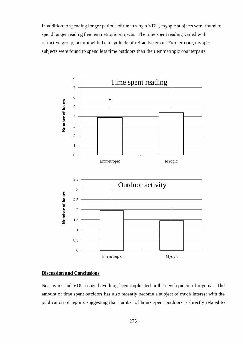
275

In addition to spending longer periods of time using a VDU, myopic subjects were found to

spend longer reading than emmetropic subjects. The time spent reading varied with

refractive group, but not with the magnitude of refractive error. Furthermore, myopic

subjects were found to spend less time outdoors than their emmetropic counterparts.

Discussion and Conclusions

Near work and VDU usage have long been implicated in the development of myopia. The

amount of time spent outdoors has also recently become a subject of much interest with the

publication of reports suggesting that number of hours spent outdoors is directly related to

0

1

2

3

4

5

6

7

8

Emmetropic Myopic

Nu

mb

er o

f h

ou

rs

Time spent reading

0

0.5

1

1.5

2

2.5

3

3.5

Emmetropic Myopic

Nu

mb

er o

f h

ou

rs

Outdoor activity

276

less myopia (Rose et al. 2008). The production of hormones, for which sunlight is essential,

are believed to be involved in myopic inhibition.

The findings presented by the current study are limited largely by number of participants,

however, the results do concur with previous literature suggesting that myopic individuals

spend less time outdoors and more time carrying out near tasks compared to emmetropic

individuals.

The principal factor in reducing myopia progression through outdoor activity has been

identified as the production of hormones such as dopamine, serotonin and melatonin. The

production of serotonin and melatonin is regulated by the pineal gland located in the central

region of the brain. The pineal gland is often referred to as the ‗third eye‘, as much of its

input is derived from the ocular photoreceptors in the retina. The retina possesses two main

types of photoreceptor: rod cells and cone cells. In an outdoors environment the cone cells

are likely to be of more importance as the pupil is more miosed and cone cells, which are

more centrally located on the retina, are required to see. Previous work investigating the

pineal gland with reference to form deprivation myopia has noted diurnal variations to the

response elicited by image degradation.

In summary, the very limited data collected as part of this study has shown a strong link

between close work and myopia. It would be of great value to have questionnaire responses

from all subjects who underwent the ocular MRI.

277

APPENDIX 4: MRI DERIVED AXIAL LENGTHS AND VOLUMES

(RIGHT EYES)

IOLMaster measurements of axial length (AL), keratometry (K) and anterior chamber depth

(ACD).

Right eye data

R AL

MRI R MSE

R

Total

Vol

R

Post

Vol

R

Ant

Vol

R AL

IOL

R

ACD

IOL

R AL

MRI -

IOL

RE

K AXIS

RE

K AXIS

28.73 -10.56 11777 10646 1131 28.12 3.71 0.61 8.2 38 7.99 128

26.62 -10.55 8908 7791 1117 26.29 3.63 0.33 7.46 20 7.28 110

25.67 -9.995 7934 7027 907 25.08

0.59 7 173 6.89 83

29.7 -9.245 10013 9033 980 27.51 3.32 2.19 8.06 3 7.71 93

26.64 -9.055 8484 7553 931 25.87 3.81 0.77 7.5 172 7.36 82

26.77 -9 9188 8028 1160 27.3 3.73 -0.53

27.13 -8.87 9533 8345 1188 26.48 3.66 0.65 7.71 46 7.62 136

25.96 -8.62 9258 7882 1376 26.64 4.01 -0.68 7.62 4 7.5 94

27.69 -8.5 9554 8625 929 26.68 3.83 1.01 7.9 176 7.61 86

26.15 -8.347 8055 7074 981 25.88 3.94 0.27 7.4 104 7.25 14

25.67 -7.12 9815 8603 1212 26.22 3.59 -0.55 7.65 128 7.59 98

28.57 -7 10745 9739 1006 27.99 3.51 0.58 8.3 17 8.12 107

26.76 -6.805 9684 8606 1078 25.72 4.39 1.04 7.47 120 7.36 90

25.68 -6.68 7562 6563 999 25.16 3.31 0.52 7.5 138 7.44 48

26.61 -6.625 10291 9081 1210 26.84 3.69 -0.23 7.99 2 7.86 92

24.63 -6.625 7721 6588 1133 25.02 3.57 -0.39 7.68 177 7.47 87

25.65 -6.55 8480 7464 1016 26.14 3.60 -0.49 7.97 178 7.85 88

25.62 -6.435 8577 7600 977 25.23 4.03 0.39 7.35 6 7.15 96

26.27 -5.75 8818 7846 972 25.81 3.15 0.46 7.53 110 7.45 20

26.62 -5.55 8419 7320 1099 25.84 3.92 0.78 7.66 171 7.58 81

25.62 -5.5 9445 8313 1132 25.77 4.07 -0.15 7.76 9 7.59 99

25.33 -5.245 8029 7220 809 25.22 3.87 0.12 7.56 2 7.39 92

26.66 -4.75 8314 7047 1267 25.94 4.02 0.72

25.74 -3.81 8014 6905 1109 24.49 3.34 1.25 7.65 10 7.13 100

26.64 -3.75 10932 9643 1289 26.35 3.9 0.29 8.32 7 8.03 97

24.74 -3.24 8528 7395 1133 25.38 3.95 -0.64 7.76 83 7.71 173

24.62 -3.183 7362 6212 1150 24.28 3.59 0.34 7.69 170 7.46 80

26.71 -3.125 8950 7986 964 25.72 3.95 0.99 7.92 151 7.84 61

24.45 -3 6724 5637 1087 23.33 3.87 1.12 7.27 1 7 91

25.67 -3 7958 6889 1069 25.3 3.7 0.37 7.89 178 7.84 88

26.65 -2.5 8918 7783 1135

24.77 -2.31 8086 6672 1414 24.84 3.91 -0.07 7.62 27 7.49 117

23.81 -2.055 7213 6046 1167 24.41 3.27 -0.6 7.93 4 7.68 94

23.11 -1.68 7262 6329 933 23.58 3.83 -0.47 7.82 128 7.53 38

25.68 -1.555 7936 6891 1045 24.55 3.84 1.13 8.01

7.91

24.49 -1.31 7857 6928 929 23.72 2.67 0.77 7.64 22 7.44 112

24.6 -0.87 7836 6926 910 23.19 3.61 1.41 7.69 178 7.52 88

24.72 -0.81 7521 6888 633 24.15 3.48 0.57 8.11 5 8.01 95

23.64 -0.75 7645 6580 1065 23.49 3.46 0.15 7.79 20 7.64 110

23.17 -0.75 7493 6526 967 23.17

0

278

23.66 -0.68 7625 6364 1261 23.41 3.31 0.25 8.05 177 7.82 87

24.04 -0.5 7657 6413 1244 23.9 3.76 0.14 7.76 4 7.58 94

24.78 -0.435 7955 6603 1352 23.54 3.69 1.24 7.61 88 7.51 178

23.69 -0.31 7479 6376 1103 22.63 3.48 1.06 7.72 1 7.49 91

24.14 -0.3 7134 6032 1102 23.86 3.66 0.28 8.07

7.9

25.64 -0.245 8361 7018 1343 24.39 3.7 1.25 8 4 7.92 94

22.96 -0.185 7670 6480 1190 22.96 3.32 0 7.93 116 7.86 26

24.04 -0.18 6845 5898 947 23.22 3.562 0.82 7.83 8 7.69 98

25.65 -0.12 7708 6393 1315 24.21 3.68 1.44 8.1 161 8.04 161

25.68 -0.06 8307 7241 1066 23.54 3.56 2.14 7.93 129 7.87 39

23.64 -0.06 7194 6079 1115 23.75 3.34 -0.11 7.77 2 7.57 92

25.65 -0.005 9285 8209 1076 24.64 3.68 1.01 8.14 177 7.9 87

23.61 0 8021 6989 1032

23.25 0 8658 7236 1422 24.09 3.04 -0.84 8.01 16 7.82 106

25.67 0.12 9052 7972 1080 25.26 3.17 0.41 8.48 162 8.27 72

24.71 0.173 8337 7171 1167 24.43 3.57 0.28 8.2

8.05

23.68 0.19 6909 5747 1162 23.22 3.09 0.46 8.06 28 7.98 118

25.67 0.19 8478 7432 1046 23.56 3.09 2.11 8.42 170 8.22 80

24.7 0.245 7995 6841 1154 23.53 3.53 1.17 7.72 1 7.49 91

24.62 0.25 8464 7313 1151 24.34 3.53 0.28 7.99 83 7.92 173

23.61 0.37 7738 6513 1225 23.27 3.13 0.34 7.88 135 7.8 45

22.65 0.435 6598 5547 1051 22.44 3.32 0.21 7.5 2 7.24 92

23.73 0.5 7268 6222 1046 23.4 3.48 0.33 7.97 10 7.85 100

23.78 0.5 8293 7202 1091 23.81 3.68 -0.03 8.06 172 7.87 82

23.62 0.56 7318 6126 1192 22.85 3.362 0.77 7.72 102 7.7 12

24.6 1.185 7780 6666 1114 22.83 3.16 1.77 7.94 171 7.87 81

21.6 1.495 6615 5525 1090 21.72 3.5 -0.12 7.88 2 7.54 92

24.63 1.56 7445 6232 1213 23.47 3.59 1.16 7.72 135 7.69 45

22.85 2.685 7661 6612 1049 22.89 3.26 -0.04 8.5 14 8.02 104

22.9 3.25 6584 5455 1129 22.59 3.54 0.31 7.86 5 7.77 95

21.6 3.815 6895 5830 1065 22.22 3.31 -0.62 8 12 7.44 102

21.65 4.375 5036 4017 1019 21.75 3.47 -0.1 7.65 136 7.57 46

20.91 9.5 5586 4510 1076 20.32 3.38 0.59

279

Radius band averages for each refractive group

EMM: Emmetropes

LM: Low Myopes

HM: High Myopes

HYP: Hyperopes

SD: Standard Deviation

Dist along geometric axis (%) EMM EMM SD LM LM SD HM HM SD HYP HYP SD

1 8.123 0.688 7.958 0.710 7.545 0.596 8.341 1.637

2 16.041 1.397 16.024 1.485 15.202 1.340 16.025 2.253

3 15.748 1.929 16.093 1.510 15.127 1.716 15.890 1.801

4 15.990 2.577 16.337 1.886 14.722 2.232 15.828 2.051

5 16.057 3.435 16.509 2.846 14.422 4.048 15.350 3.880

6 15.569 5.128 15.302 3.880 12.609 4.633 14.791 6.069

7 12.531 5.641 15.316 4.233 12.414 5.471 14.939 6.198

8 12.521 5.689 14.994 4.848 12.691 6.137 15.339 6.635

9 11.870 4.717 14.978 5.898 12.364 5.935 14.792 6.067

10 12.031 4.613 14.711 4.511 11.413 3.885 14.520 5.796

11 11.753 3.049 13.366 3.290 11.141 2.494 13.502 5.929

12 11.907 1.692 12.326 1.718 11.623 2.109 10.829 2.215

13 12.257 1.237 12.431 1.187 12.039 1.592 11.055 1.666

14 12.662 1.099 12.811 1.214 12.731 1.339 11.393 1.542

15 13.092 0.918 12.965 1.170 13.042 0.916 12.015 1.062

16 13.363 0.948 13.072 0.757 13.439 0.846 12.380 1.386

17 13.297 0.703 12.995 0.701 13.557 0.908 12.193 1.216

18 13.333 0.860 13.158 0.702 13.673 0.759 12.378 1.349

19 13.384 0.721 13.204 0.669 13.648 0.871 12.550 1.208

20 13.509 0.721 13.300 0.594 13.511 0.771 12.789 1.176

21 13.450 0.614 13.273 0.595 13.532 0.889 12.692 1.116

22 13.245 0.693 13.334 0.516 13.483 0.829 12.973 1.309

280

23 13.344 0.661 13.258 0.527 13.453 0.787 13.027 0.951

24 13.302 0.616 13.115 0.603 13.490 0.962 12.699 1.131

25 13.287 0.626 13.218 0.554 13.286 0.852 12.619 0.961

26 13.148 0.554 13.271 0.481 13.149 0.689 12.707 0.773

27 13.216 0.522 13.264 0.551 13.337 0.850 12.946 0.774

28 13.182 0.637 12.956 0.712 13.298 0.895 12.352 0.773

29 13.140 0.561 13.160 0.551 13.276 0.942 12.539 0.803

30 13.045 0.557 13.225 0.516 13.263 0.822 12.359 1.036

31 13.093 0.453 12.984 0.606 13.184 0.681 12.556 0.753

32 13.138 0.600 13.146 0.533 13.309 0.893 12.155 0.734

33 13.080 0.719 13.191 0.487 13.282 0.948 12.369 0.830

34 12.916 0.584 13.035 0.505 13.526 0.801 12.206 0.815

35 13.113 0.551 13.192 0.424 13.229 0.751 12.415 0.713

36 13.039 0.617 13.020 0.559 13.192 0.732 12.057 0.884

37 13.033 0.754 13.152 0.531 13.438 0.796 12.170 0.800

38 12.926 0.663 13.057 0.557 13.530 0.752 12.592 1.092

39 13.154 0.576 13.055 0.581 13.500 0.870 12.001 0.586

40 13.104 0.629 13.149 0.630 13.373 0.734 12.201 1.066

41 12.900 0.601 13.201 0.662 13.384 0.818 12.564 1.016

42 13.062 0.715 12.904 0.562 13.460 0.728 11.803 0.612

43 13.155 0.487 13.116 0.439 13.431 0.989 12.506 0.892

44 12.985 0.564 13.032 0.813 13.429 0.767 12.347 0.741

45 12.972 0.692 13.143 0.723 13.605 0.746 11.873 0.824

46 13.130 0.520 13.105 0.526 13.259 0.855 12.399 0.869

47 13.008 0.504 13.080 0.604 13.366 0.956 12.104 0.805

48 12.944 0.540 12.980 0.456 13.438 0.834 12.033 0.739

49 13.024 0.417 13.113 0.632 13.650 0.739 12.364 0.883

50 13.046 0.534 13.065 0.560 13.283 0.729 12.186 0.944

51 12.937 0.703 13.100 0.428 13.237 1.127 12.165 0.642

52 12.974 0.430 13.094 0.511 13.608 0.779 12.201 0.874

53 13.104 0.458 12.929 0.801 13.526 0.641 12.002 0.656

54 12.995 0.641 13.178 0.410 13.324 0.704 12.313 0.718

55 12.903 0.493 13.064 0.367 13.394 1.120 12.234 0.783

56 12.982 0.461 12.972 0.764 13.375 0.791 12.049 0.997

57 13.197 0.593 13.183 0.751 13.605 0.734 12.159 0.631

281

58 12.902 0.611 13.039 0.373 13.315 0.737 12.488 0.926

59 12.908 0.564 13.002 0.651 13.429 1.016 12.050 0.693

60 13.160 0.604 13.108 0.667 13.401 0.688 11.833 0.679

61 12.941 0.601 13.198 0.488 13.400 0.702 12.666 0.970

62 12.895 0.660 13.005 0.623 13.506 0.910 12.197 0.953

63 13.097 0.496 13.154 0.637 13.166 0.918 12.244 0.859

64 13.109 0.620 13.110 0.461 13.701 0.667 12.163 0.961

65 12.919 0.516 13.058 0.489 13.189 0.579 12.160 0.818

66 12.943 0.532 13.167 0.691 13.497 0.882 12.597 1.079

67 13.149 0.553 13.160 0.465 13.439 0.937 12.093 1.034

68 12.990 0.470 13.055 0.635 13.377 0.748 12.110 0.793

69 13.028 0.534 13.203 0.658 13.394 0.752 12.356 0.800

70 13.174 0.568 13.133 0.477 13.214 0.681 12.378 0.773

71 13.096 0.601 13.150 0.663 13.482 0.769 12.441 0.833

72 13.158 0.516 13.274 0.751 13.437 0.906 12.160 0.695

73 13.147 0.777 13.228 0.407 13.302 0.818 12.415 0.619

74 13.167 0.457 13.258 0.533 13.398 0.707 12.715 1.146

75 13.171 0.585 13.213 0.513 13.482 0.750 12.360 0.836

76 13.160 0.575 13.401 0.615 13.374 0.754 12.475 0.769

77 13.339 0.564 13.172 0.571 13.257 1.005 12.754 0.880

78 13.179 0.551 13.397 0.373 13.451 0.859 12.691 0.743

79 13.360 0.614 13.325 0.634 13.334 0.860 12.448 0.637

80 13.432 0.580 13.398 0.638 13.243 0.827 12.513 0.820

81 13.379 0.514 13.512 0.519 13.222 0.929 12.668 0.618

82 13.489 0.624 13.520 0.659 13.401 0.962 12.783 0.759

83 13.476 0.683 13.586 0.590 13.329 0.804 12.859 0.817

84 13.662 0.634 13.506 0.668 13.428 1.041 12.826 0.664

85 13.644 0.590 13.619 0.703 13.427 1.027 12.814 0.648

86 13.658 0.675 13.676 0.724 13.318 1.127 13.190 0.856

87 13.820 0.689 13.769 0.936 13.403 1.087 13.042 0.981

88 13.924 0.675 13.693 0.951 13.367 1.201 13.044 0.939

89 13.967 0.732 13.639 1.014 13.291 1.213 13.409 0.989

90 13.998 0.679 13.683 1.145 13.197 1.185 13.355 0.651

91 14.057 0.879 13.697 1.336 13.217 1.330 13.663 1.289

282

APPENDIX 5: QUADRANT DATA FOR MRI WORK

The pages that follow provide various parameters for both XQ and +Q. The table below outlines the data provided for each set of quadrants

MSE X^2 Post

25% X^2 25-75 X^2 25-75 IV Post 25%

IV NASAL

25-75

IV TEMP

25-75

Ratio MAX NT

Dist:AL

Mean Post

Volume

Mean Axial

Length

Mean

Sph Error

X^2

coefficient

of the

second

order

polynomial

curve fitted

to data

comprising

the

posterior

25% of the

eye

X^2

coefficient of

the second

order

polynomial

curve fitted to

data

comprising the

region 25-75%

for a particular

quadrant

X^2

coefficient of

the second

order

polynomial

curve fitted to

data

comprising

the region 25-

75% for a

particular

quadrant

Interval

Variance for

the data

comprising

the posterior

25%

Interval

Variance for

the data

comprising

the posterior

25% for a

particular

quadrant

Interval

Variance for

the data

comprising

the posterior

25% for a

particular

quadrant

The ratio between

the maximum

distances of two

parallel quadrants

The mean

volume of the

posterior 25% of

the eye in mm³

The mean axial

length of the

two

corresponding

quadrants

283

NASAL-TEMPORAL QUADRANT DATA

MSE X^2 Post

25%

X^2 NASAL

25-75

X^2 TEMP

25-75 IV Post 25%

IV NASAL

25-75

IV TEMP

25-75

Ratio MAX NT

Dist:AL

Mean Post

Volume

Mean Axial

Length

-10.56 -0.0382 -0.0355 0.0311 6.550214061 1.017000102 1.035565102 1.063288133 1954.473606 27.57697588

-10.555 -0.055 -0.0399 0.0382 5.221370344 0.997084097 1.045796015 0.960608753 1245.113054 26.4110575

-9.995 -0.0582 -0.0356 0.0407 5.370571971 0.92934619 1.282087798 0.960734886 1087.61731 25.39215735

-9.245 -0.0538 -0.0332 0.0386 5.313963754 1.019177441 1.186803833 0.931321622 1532.75652 28.9819616

-9.055 -0.0561 -0.0391 0.0404 5.066020037 1.001759781 1.206774848 0.937107014 1213.635977 26.33453805

-9 -0.0509 -0.04 0.0458 5.386507893 1.045711087 1.348732936 0.997856332 1382.473106 26.77239905

-8.87 -0.0484 -0.036 0.0384 5.56326608 0.986234326 1.196912891 0.997109511 1491.692501 27.11829538

-8.62 -0.0455 -0.0363 0.0378 5.727914909 0.872267812 1.097907912 1.009724523 1444.193808 25.8713142

-8.5 -0.0515 -0.0344 0.0441 5.558711213 0.929034146 1.542703863 0.938289495 143.6286976 27.44885788

-8.347 -0.0521 -0.0421 0.047 5.209295959 0.961180097 1.232310873 0.982202369 1221.778608 25.4633285

-7.12 -0.0458 -0.0417 0.0373 5.573012947 0.957788128 0.96034608 1.039179761 1431.062105 25.83818674

-7 -0.0453 -0.0402 0.0503 5.804556666 1.152583872 1.579369372 1.01011167 1704.243664 28.04238825

-6.805 -0.0419 -0.0511 0.0448 6.027823824 1.401075669 1.392970028 1.0511904 1610.813872 26.21982235

-6.68 -0.0571 -0.0382 0.0477 4.923698161 0.876902552 1.051663982 0.946995844 1113.119265 25.44420914

-6.625 -0.0507 -0.0388 0.0349 5.530258188 1.078573039 0.963188896 1.023307259 1341.340185 26.31924945

-6.625 -0.0575 9.4569 0.0444 4.804890961 0.998866665 0.974696491 1.01008123 1007.308287 24.28931005

-6.55 -0.0499 -0.0373 0.0375 5.400457345 0.955841974 1.003815235 0.993595646 1368.965429 26.3782856

-6.435 -0.0463 -0.0402 0.0432 16.33378095 0.98842505 1.066672065 1.006243989 1410.731587 25.7936465

-5.75 -0.0453 -0.0378 0.0422 5.655597367 0.911647275 1.020281935 1.045085826 1387.338773 25.301159

-5.55 -0.0484 -0.0376 0.0428 5.308229868 0.946007633 1.200225338 0.982458043 1383.001058 26.1116304

-5.5 -0.0464 -0.0423 0.0427 5.55157812 1.090905432 1.001961915 1.051818185 1356.413646 25.3194996

-5.245 -0.0508 -0.0406 0.0331 5.299620199 0.953803244 1.097891169 0.988693241 1236.339795 25.29302849

-4.75 -0.0563 -0.0435 0.043 5.153052477 1.106074031 1.296196489 0.962426893 1220.716888 26.45828722

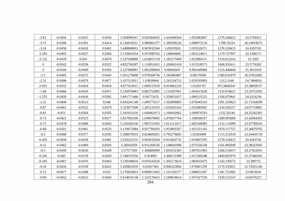
284

-3.81 -0.0456 -0.0433 0.0504 5.594099547 0.926366945 1.441840564 1.055083607 1279.246612 24.3758412

-3.75 -0.0396 -0.0391 0.0414 6.136918551 0.980081377 1.389299226 1.080072116 1708.19224 26.24919675

-3.24 -0.0458 -0.0418 0.0481 5.488888001 0.903932504 1.45919926 1.035520371 1278.318415 24.4203742

-3.183 -0.0493 -0.0437 0.0366 5.133601854 0.947890763 1.188606881 1.003124811 1179.727997 24.3396571

-3.125 -0.0478 -0.041 0.0479 5.537569899 1.016857119 1.185377409 1.052994151 1319.912242 25.3505

-3 -0.0542 -0.0558 0.0522 4.852704587 1.110952452 1.209062418 1.015538573 1006.933611 23.5776282

-3 -0.0544 -0.0409 0.0393 5.227989991 1.092280004 0.99045647 0.995449986 1155.448446 25.3031616

-2.5 -0.0495 -0.0375 0.0443 5.501279088 0.979268736 1.183481887 0.98178588 1380.031879 26.37832482

-2.31 -0.0496 -0.0479 0.0477 5.337513011 1.03830064 1.241324753 1.020195983 1212.3146 24.7484816

-2.055 -0.0552 -0.0424 0.0454 4.877452912 1.008157619 0.919602233 1.03292767 972.9840347 23.38958137

-1.68 -0.0466 -0.0429 0.0471 5.136978483 0.805753085 1.116397061 1.063015638 1124.918621 23.10753205

-1.555 -0.0428 -0.0436 0.0392 5.891771468 0.94775476 1.359021027 1.080125525 1356.879441 24.3216239

-1.31 -0.0408 -0.0515 0.048 6.043241148 1.499773317 1.562808895 1.076445516 1591.210923 25.71544299

-0.87 -0.0461 -0.0522 0.0479 5.323877608 1.205124193 1.020265343 1.052985692 1234.592257 24.07754981

-0.81 -0.051 -0.0364 0.0505 5.101653316 1.049461073 1.100042062 1.049976763 1132.56144 24.25582365

-0.75 -0.0421 -0.0525 0.0477 5.837992506 1.049079845 1.476957764 1.108500197 1280.093606 23.42944305

-0.75 -0.0478 -0.0488 0.0443 5.326304336 1.003723393 1.011111617 1.065548483 1132.113098 23.47788163

-0.68 -0.0501 -0.0461 0.0533 5.119672984 0.927784393 1.053093567 1.051551165 1070.117757 23.36870795

-0.5 -0.0488 -0.0377 0.0395 5.308970933 0.824669201 0.795274685 1.03504409 1115.212018 23.54445729

-0.435 -0.0458 -0.0418 0.0481 5.510223155 0.903932504 0.912820735 1.034097293 1278.318415 24.4203742

-0.31 -0.0462 -0.0469 0.0503 5.36042028 0.931269526 1.148641098 1.075536258 1161.895049 23.38322945

-0.3 -0.0456 -0.0636 0.0449 5.37577299 1.366800999 1.003552383 1.087831983 1268.216017 24.27052055

-0.245 -0.045 -0.0378 0.0429 5.748370356 0.924901 1.384572398 1.011369348 1404.691979 25.37446305

-0.185 -0.0467 -0.0476 0.0463 5.539188634 0.935543526 1.305173633 1.083033475 1142.239572 23.309722

-0.18 -0.0434 -0.0339 0.0422 5.439852059 0.65927463 0.996322894 1.070667299 1170.353051 22.74591246

-0.12 -0.0477 -0.0388 0.052 5.170920823 0.896911692 1.151195577 1.048651587 1181.751002 23.9619541

-0.06 -0.0452 -0.0512 0.0443 5.614016136 1.133176415 1.249814614 1.057427539 1320.513147 24.6570227

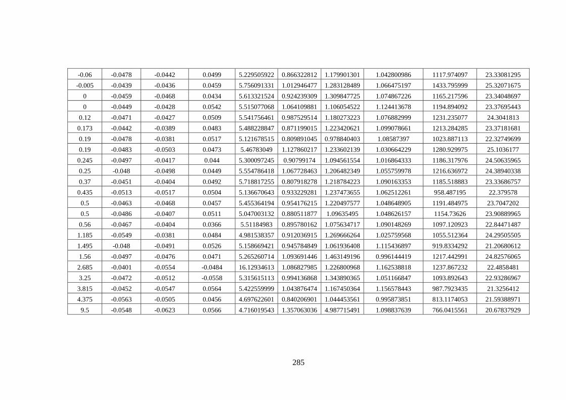
285

-0.06 -0.0478 -0.0442 0.0499 5.229505922 0.866322812 1.179901301 1.042800986 1117.974097 23.33081295

-0.005 -0.0439 -0.0436 0.0459 5.756091331 1.012946477 1.283128489 1.066475197 1433.795999 25.32071675

0 -0.0459 -0.0468 0.0434 5.613321524 0.924239309 1.309847725 1.074867226 1165.217596 23.34048697

0 -0.0449 -0.0428 0.0542 5.515077068 1.064109881 1.106054522 1.124413678 1194.894092 23.37695443

0.12 -0.0471 -0.0427 0.0509 5.541756461 0.987529514 1.180273223 1.076882999 1231.235077 24.3041813

0.173 -0.0442 -0.0389 0.0483 5.488228847 0.871199015 1.223420621 1.099078661 1213.284285 23.37181681

0.19 -0.0478 -0.0381 0.0517 5.121678515 0.809891045 0.978840403 1.08587397 1023.887113 22.32749699

0.19 -0.0483 -0.0503 0.0473 5.46783049 1.127860217 1.233602139 1.030664229 1280.929975 25.1036177

0.245 -0.0497 -0.0417 0.044 5.300097245 0.90799174 1.094561554 1.016864333 1186.317976 24.50635965

0.25 -0.048 -0.0498 0.0449 5.554786418 1.067728463 1.206482349 1.055759978 1216.636972 24.38940338

0.37 -0.0451 -0.0404 0.0492 5.718817255 0.807918278 1.218784223 1.090163353 1185.518883 23.33686757

0.435 -0.0513 -0.0517 0.0504 5.136670643 0.933229281 1.237473655 1.062512261 958.487195 22.379578

0.5 -0.0463 -0.0468 0.0457 5.455364194 0.954176215 1.220497577 1.048648905 1191.484975 23.7047202

0.5 -0.0486 -0.0407 0.0511 5.047003132 0.880511877 1.09635495 1.048626157 1154.73626 23.90889965

0.56 -0.0467 -0.0404 0.0366 5.51184983 0.895780162 1.075634717 1.090148269 1097.120923 22.84471487

1.185 -0.0549 -0.0381 0.0484 4.981538357 0.912036915 1.269666264 1.025759568 1055.512364 24.29505505

1.495 -0.048 -0.0491 0.0526 5.158669421 0.945784849 1.061936408 1.115436897 919.8334292 21.20680612

1.56 -0.0497 -0.0476 0.0471 5.265260714 1.093691446 1.463149196 0.996144419 1217.442991 24.82576065

2.685 -0.0401 -0.0554 -0.0484 16.12934613 1.086827985 1.226800968 1.162538818 1237.867232 22.4858481

3.25 -0.0472 -0.0512 -0.0558 5.315615113 0.994136868 1.343890365 1.051166847 1093.892643 22.93286967

3.815 -0.0452 -0.0547 0.0564 5.422559999 1.043876474 1.167450364 1.156578443 987.7923435 21.3256412

4.375 -0.0563 -0.0505 0.0456 4.697622601 0.840206901 1.044453561 0.995873851 813.1174053 21.59388971

9.5 -0.0548 -0.0623 0.0566 4.716019543 1.357063036 4.987715491 1.098837639 766.0415561 20.67837929

286

SUPERIOR-INFERIOR QUADRANT DATA

MSE X^2 Post

25%

X^2 SUP 25-

75

X^2 INF 25-

75 IV Post 25%

IV SUP 25-

75

IV INF 25-

75

Ratio MAX SI

Dist:AL

Posterior 25%

Vol

Mean Axial

Length

-10.56 -0.0438 -0.0348 0.0289 6.18937828 1.132587517 0.948517767 1.064964546 1695.158975 27.50060985

-10.555 -0.047 -0.0444 0.0364 5.5882157 1.149548037 1.131253109 0.995449461 1453.926191 26.38275605

-9.995 -0.0481 -0.0428 0.0368 5.734519913 1.32476912 0.958445821 1.022683074 1273.939098 24.9831344

-9.245 -0.059 -0.0383 0.0376 5.062183006 1.209516796 1.137648898 0.887933922 1413.762295 29.14836881

-9.055 -0.0505 -0.0459 0.0444 5.596163954 1.280129565 1.247238466 0.987690822 1350.573123 26.35753509

-9 -0.0563 -0.0424 0.0455 5.179297109 1.128491394 1.154003933 0.972598427 1251.274622 26.78740035

-8.87 -0.0494 -0.0393 0.0373 5.48132114 1.224121803 0.989006991 0.998451339 1449.891679 27.01041805

-8.62 -0.0496 -0.0411 0.089 5.493286845 1.059186127 0.955575902 0.846681164 1323.798981 25.8613929

-8.5 -0.0468 -0.0453 0.0397 5.425288668 1.491973759 1.032590876 0.995030743 1572.651742 27.38036665

-8.347 -0.0557 -0.0488 0.0502 5.047543227 1.176014525 1.168868061 0.974139778 1144.991163 25.4875868

-7.12 -0.0451 -0.0413 0.0383 5.60762112 0.976614701 0.971843004 1.050210207 1432.518486 25.65301655

-7 -0.0491 -0.0454 0.0459 5.657332197 1.382141324 1.344094584 0.983679164 1579.516445 28.10624805

-6.805 -0.0434 -0.0479 0.046 5.774766223 1.294041215 1.29896106 1.032713215 1558.00086 26.24392356

-6.68 -0.0589 -0.0448 0.0464 4.835816793 1.036115405 1.0844057 0.950173402 1073.101927 25.37337205

-6.625 -0.048 -0.0423 0.0398 5.504981274 1.157520283 1.035839259 1.046496878 1416.645564 26.31790255

-6.625 -0.0554 -0.0488 0.0408 4.855555057 1.089442457 0.988575482 1.019586387 1046.221121 24.29778455

-6.55 -0.05 -0.0386 0.0415 5.388832141 1.047283234 1.084939526 1.004333471 1365.244715 26.3687964

-6.435 -0.049 -0.042 0.0453 5.439220811 1.115533394 1.220755269 0.998124733 1317.179623 25.64015195

-5.75 -0.0439 -0.0462 0.0448 5.63337695 1.085338594 1.170373871 1.0751082 1430.500088 25.29159725

-5.55 -0.05 -0.0441 0.0401 5.327827457 1.168702411 1.067764693 0.970427422 1350.167915 26.222793

-5.5 -0.0441 -0.0439 0.042 5.753655304 1.155903482 0.980094184 1.063305507 1423.05031 25.28305065

-5.245 -0.0476 -0.0426 0.0438 5.508128673 1.185540707 1.027667346 1.017229609 1320.173276 25.29991125

-4.75 -0.0555 -0.0479 0.0401 5.095530283 1.267044408 1.129525766 0.955448335 1234.593697 26.41852535

-3.81 -0.0483 -0.0469 0.0456 5.455554596 1.201917661 1.016438673 1.048606654 1207.916293 24.37766125

287

-3.75 -0.0442 -0.0418 0.0409 5.830012869 1.077071845 0.996893995 1.060429186 1509.567889 26.06978875

-3.24 -0.0439 -0.0456 0.051 5.712040891 1.252376592 1.180189279 1.053093236 1345.722067 24.53070331

-3.183 -0.0496 -0.0464 0.0507 5.085460775 1.036925399 1.112862923 1.030880527 1163.699507 24.24718445

-3.125 -0.0502 -0.0408 0.0444 5.262459648 0.970839105 1.09832483 1.024541227 1255.366063 25.33594475

-3 -0.051 -0.0548 0.0523 5.133114605 1.227326315 1.148288798 1.027596475 1077.865313 23.66286843

-3 -0.0471 -0.0393 0.0402 5.447599487 1.028551511 0.939495741 1.023456235 1334.714037 25.3048997

-2.5 -0.0508 -0.042 0.0383 5.226452281 1.062164987 0.905112438 0.989126724 1337.394703 26.3064175

-2.31 -0.0476 -0.0443 0.056 5.521178257 1.12363291 1.228707412 1.055636218 1274.520354 24.85861435

-2.055 -0.0539 -0.0386 0.0419 4.812756275 0.76372326 0.835858814 1.040550596 977.4436343 23.1654263

-1.68 -0.0433 -0.0548 0.0507 5.475057979 1.124051085 1.046188086 1.091668377 1231.836226 23.30883067

-1.555 -0.0438 -0.0444 0.049 5.855974056 1.256584197 1.110742284 1.082188736 1326.281991 24.32512297

-1.31 -0.0448 -0.0461 0.0519 5.741427166 1.497408781 1.442604519 1.028333032 1446.739703 25.69415028

-0.87 -0.0418 -0.057 0.0575 5.588070092 1.605627142 1.209450681 1.111610395 1335.819268 23.84855365

-0.81 -0.0499 -0.0506 0.0434 5.235681641 1.120894755 1.170699043 1.064124177 1154.212007 24.22105855

-0.75 -0.0455 -0.0427 0.0522 5.516193071 1.016468484 1.218743245 1.059812758 1185.280584 23.4377726

-0.75 -0.0464 -0.0491 0.0437 5.108491568 1.097198016 0.929516836 1.0768077 1158.526298 23.3997917

-0.68 -0.0447 -0.0484 0.0528 5.574884461 1.052407279 1.295215432 1.092161517 1203.939021 23.4129458

-0.5 -0.0475 -0.0463 0.0453 5.310106929 0.997464963 0.907774964 1.067773196 1143.128371 23.51767365

-0.435 -0.0444 -0.0456 0.051 5.741385717 1.252376592 1.180189279 1.053763952 1330.567539 24.53070331

-0.31 -0.0458 -0.0522 0.0408 5.517168605 1.190760927 0.864124422 1.062619208 1178.860255 23.45113975

-0.3 -0.0455 -0.0455 0.0507 5.396924859 1.040153853 1.103498686 1.051570117 1283.856481 24.39293115

-0.245 -0.0478 -0.0402 0.0372 5.534520765 1.064067931 0.976583171 0.986187814 1320.412378 25.3553024

-0.185 -0.0458 -0.0518 0.0421 5.665784396 1.37965268 0.875793541 1.090144274 1165.112138 23.31399265

-0.18 -0.0406 -0.0489 0.0428 5.662937883 0.951697365 0.780961599 1.156149948 1222.482251 22.4845578

-0.12 -0.0473 -0.053 0.0494 5.239980072 1.156150303 1.085294428 1.064276596 1201.882005 24.06365207

-0.06 -0.0432 -0.0479 0.054 5.710688223 1.192949427 1.251964188 1.061710112 1385.823114 24.6942492

-0.06 -0.0451 -0.0508 0.0608 5.369125605 1.046399236 1.227455515 1.085026516 1177.338528 23.2562133

288

-0.005 -0.0421 -0.049 0.048 5.991530138 1.309383968 1.205404546 1.075655815 1500.229253 25.36412679

0 -0.0445 -0.0502 0.0557 5.624675982 1.375098891 1.163218879 1.106271076 1202.336457 23.34495635

0 -0.0472 -0.0474 0.0453 4.936053384 1.099670112 0.890398781 1.133488647 1127.421195 23.2816711

0.12 -0.0425 -0.0471 0.054 5.793954995 1.199539021 1.176003709 1.132839829 1364.491279 24.30411995

0.173 -0.0431 -0.0461 0.0511 5.329584232 1.015369739 1.47943599 1.123072204 1244.492395 23.37409535

0.19 -0.0501 -0.0533 0.0488 4.721666002 1.009701024 0.859819311 1.120212588 959.9643482 22.13331515

0.19 -0.0431 -0.0486 0.051 5.636023124 1.180984892 1.231586649 1.059633367 1438.650951 25.13138402

0.245 -0.0462 -0.0455 0.0473 5.450170644 1.029926999 1.032209286 1.061219514 1268.628275 24.43364355

0.25 -0.0431 -0.0442 0.0485 5.807480037 1.118969829 1.134225411 1.078680546 1351.368628 24.3571014

0.37 -0.0491 -0.0474 0.0474 5.307622629 1.025250105 0.979109345 1.064138469 1090.190451 23.35027425

0.435 -0.0452 -0.0531 0.0512 5.491804635 1.180789158 0.995616329 1.104484784 1093.143983 22.434064

0.5 -0.0478 -0.0444 0.0401 5.395095005 1.088157413 0.912844892 1.016282462 1154.195566 23.7057501

0.5 -0.042 -0.0495 0.0465 5.297522277 1.035796084 1.381606462 1.139385582 1314.183943 23.71115865

0.56 -0.0395 -0.0506 0.0453 5.548834222 1.163812546 1.076438709 1.152591511 1271.433921 22.6175468

1.185 -0.0591 -0.0471 0.0412 4.760533953 1.248714094 0.990031784 1.015258726 980.829785 24.29912393

1.495 -0.0442 -0.0558 0.0438 5.142831495 2.198017263 2.233250869 1.163502053 1007.194079 21.2945158

1.56 -0.0482 -0.0506 0.0479 5.318154944 1.386478243 1.146378899 1.001738142 1253.76122 24.8102413

2.685 -0.0448 -0.0557 -0.0549 5.448122262 1.155848993 1.01786485 1.116060521 1120.697693 22.61430779

3.25 -0.0492 -0.0555 0.0522 4.845816916 1.250154335 1.078092971 1.044531019 1041.470342 22.84578355

3.815 -0.0448 -0.0564 0.0363 5.396280591 1.030435941 0.689610167 1.157561519 996.0648241 21.319787

4.375 -0.0515 -0.0527 0.0491 4.715486958 1.057115909 0.9579836 1.030304885 882.1330372 21.5115008

9.5 -0.049 -0.0524 0.0563 4.601325628 1.896587161 2.515601567 1.130528969 838.5197058 20.4576022

289

SUPERIOR-TEMPORAL AND INFERIOR-NASAL QUADRANT DATA

MSE X^2 Post

25%

X^2 SUP

TEMP 25-75

X^2 INF

NASAL 25-

75

IV Post 25% IV IN 25-75 IV ST 25-75 Ratio MAX ST-IN

Dist:AL

Mean Post

Volume

Mean Axial

Length

-10.56 -0.0402 -0.0357 0.0358 6.183303688 1.076447456 1.015446558 1.053169612 1867.862122 27.65575295

-10.555 -0.051 -0.0405 0.038 5.371023074 1.075421583 0.969601631 0.975149187 1341.140579 26.39503805

-9.995 -0.0483 -0.00456 0.0371 5.640603802 5.732493216 0.977001272 0.993380693 1312.190959 25.408097

-9.245 -0.0527 -0.0407 0.0353 5.315069165 1.235320746 1.109562574 0.927202928 1565.983417 28.99338615

-9.055 -0.0525 -0.0434 0.0386 5.40046625 1.243806444 1.055228705 0.96697587 1297.091947 26.33692615

-9 -0.0517 -0.0437 0.0392 5.444247413 1.212339924 1.087257959 0.990431892 1361.548928 26.77700197

-8.87 -0.0478 -0.0433 0.039 5.834329743 1.289651006 1.064331725 1.030003155 1490.205698 26.93624856

-8.62 -0.0448 -0.0398 0.0365 5.775079867 1.040205063 0.890011891 1.022248109 1467.822447 25.8806883

-8.5 -0.048 -0.0462 0.032 5.687786845 1.645180249 0.939951737 0.960841175 1535.783406 27.4022142

-8.347 -0.0536 -0.0525 0.0477 5.10166257 1.254765004 1.055586844 0.980610642 1187.77231 25.4653146

-7.12 -0.0461 -0.0365 0.039 5.590480139 0.868538173 0.952922331 1.045538814 1411.090977 25.7411546

-7 -0.0478 -0.0488 0.0389 5.705821227 1.534153759 1.27534768 1.001309863 1612.239093 28.0174577

-6.805 -0.0426 -0.047 0.0517 5.877585306 1.372659159 1.394790689 1.05573966 1581.847323 26.19914595

-6.68 -0.0571 -0.0438 0.0423 5.062882288 1.115123987 0.982399667 0.950327235 1110.292353 25.41187915

-6.625 -0.0494 -0.0378 0.0353 5.539520247 0.985323274 0.970371345 1.037483658 1376.929344 26.3220285

-6.625 -0.0557 -0.0456 0.0387 4.962004395 0.98988519 0.979829828 1.011911518 1041.401896 24.30730624

-6.55 -0.0496 -0.0525 0.0477 5.515930427 1.003263547 0.936099874 1.001518862 1377.544802 26.38115207

-6.435 -0.0472 -0.0448 0.0411 5.614064271 1.343853722 1.016534938 1.002549927 1377.695233 25.73639005

-5.75 -0.0443 -0.0441 0.0377 5.715986011 1.044228066 0.889064745 1.060565321 1419.652929 25.31005025

-5.55 -0.0484 -0.0483 0.0373 5.209179938 1.17411994 0.876696656 1.015207866 1322.793445 25.5369338

-5.5 -0.0466 -0.0458 0.043 5.476695962 1.084508395 1.029168754 1.04866393 1348.8415 25.3030848

-5.245 -0.0467 -0.0342 0.0396 5.520673408 1.234472614 0.955896719 0.995158618 1404.777192 25.85009936

-4.75 -0.0552 -0.0477 0.0419 5.186749345 1.279647255 1.077457133 0.969566209 1244.389393 26.4513439

290

-3.81 -0.0445 -0.0535 0.0426 5.371237251 1.107518675 0.94829885 1.098896503 1240.060199 23.70835615

-3.75 -0.0448 -0.0406 0.0384 6.028859791 1.106999489 0.959801253 1.077949309 1498.756425 26.1519808

-3.24 -0.0468 -0.0473 0.0423 5.310551367 1.064901152 0.936987137 1.065643043 1273.133143 24.6354155

-3.183 -0.0493 -0.0451 0.043 5.168199655 1.082359879 0.949332193 1.008337615 1182.756311 24.37087654

-3.125 -0.0494 -0.0427 0.0522 5.399666806 0.957005852 1.238730616 1.039125452 1298.158043 25.35023395

-3 -0.0518 -0.0508 0.0529 5.052371064 1.350594504 1.079008925 1.005136976 1074.327029 23.808563

-3 -0.0486 -0.0361 0.0361 5.263919544 0.850638814 0.930804798 1.022288539 1252.454316 24.8999878

-2.5 -0.049 -0.0525 0.0477 5.230621593 0.978873047 0.755079164 1.054189011 1216.926275 24.6450797

-2.31 -0.0478 -0.0454 0.0515 5.516158884 1.193310202 1.135664968 1.047658381 1266.616768 24.8334248

-2.055 -0.055 -0.0427 0.0358 4.874748375 0.888521929 1.020988094 1.034000058 962.6902126 23.22333975

-1.68 -0.0439 -0.0268 -0.026 5.564239386 0.961494538 0.857281011 1.102076246 1202.126612 23.185017

-1.555 -0.0405 -0.0479 0.0418 5.617074659 1.18362505 0.911676552 1.11062513 1421.013851 24.21178005

-1.31 -0.0426 -0.0532 0.0541 5.551301315 1.27785663 1.239892401 1.090518847 1378.380764 24.45622685

-0.87 -0.0432 -0.0509 0.05 5.548236063 1.146720177 1.113300971 1.137446294 1166.099446 22.65216523

-0.81 -0.0502 -0.0482 0.0402 5.273621372 1.133884882 1.135023304 1.045105394 1173.610391 24.4970554

-0.75 -0.0419 -0.0435 0.0486 5.788175309 1.010730294 0.988622833 1.138953656 1165.648381 22.3044155

-0.75 -0.0462 -0.044 0.0461 5.39447911 0.941118903 0.93437042 1.076328605 1169.40154 23.4586422

-0.68 -0.05 -0.048 0.0466 5.153515055 1.09431824 0.959913624 1.048075571 1072.824247 23.37487759

-0.5 -0.0467 -0.0381 0.0365 5.108386373 0.777537397 0.777209956 1.054038145 1154.187471 23.43131545

-0.435 -0.044 -0.044 -0.046 5.624274334 1.354984346 1.332089887 1.048901045 1337.662787 24.48497776

-0.31 -0.0441 -0.0534 0.0411 5.669389487 1.234235639 0.837761859 1.082765111 1223.731197 23.44565464

-0.3 -0.0421 -0.0444 0.0563 5.465821043 1.051729675 1.226717652 1.090915968 1311.266002 23.713

-0.245 -0.0453 -0.0406 0.0361 5.669660285 1.203617425 0.883644828 1.003855986 1392.755953 25.35050793

-0.185 -0.0452 -0.0498 0.0443 5.705089725 1.378841913 0.888533741 1.097592945 1181.150332 23.3196409

-0.18 -0.0407 -0.0491 0.0378 16.29596869 1.020942068 0.737512991 1.130073124 1221.915039 22.50700785

-0.12 -0.0477 -0.0526 0.0438 5.251491177 1.122035491 1.044977203 1.061824132 1189.091079 24.036255

-0.06 -0.0443 -0.044 0.0523 5.722887155 1.21619745 1.151692133 1.055653144 1352.434099 24.70358438

291

-0.06 -0.0469 -0.0497 0.048 5.39156866 1.105305381 0.947127891 1.062384312 1137.404717 23.31009195

-0.005 -0.0437 -0.046 0.0451 5.850877591 1.32233049 5.334730107 1.069210311 1441.062943 25.3269123

0 -0.051 -0.0525 0.0477 5.755495645 1.339516588 1.059670706 1.113039675 1049.86345 23.35347695

0 -0.0465 -0.0503 0.0427 5.304835032 1.043351728 0.944575134 1.124746051 1148.844536 23.32690715

0.12 -0.0442 -0.0477 0.0454 5.793036588 1.302939979 1.127549527 1.088870427 1373.658586 24.86855723

0.173 -0.045 -0.0488 0.037 5.495821579 1.186924165 0.869613107 1.074304162 1263.766959 24.0679892

0.19 -0.0483 -0.0526 0.0438 5.148193722 0.960215869 0.853110582 1.114679973 1002.961231 22.21343345

0.19 -0.0456 -0.0458 0.0487 5.614717256 1.170908501 1.100285186 1.043859223 1353.561775 25.07387836

0.245 -0.0464 -0.0492 0.0427 6.274518331 1.136597022 0.946825032 1.054346042 1267.224049 24.4729175

0.25 -0.0443 -0.0451 0.0519 5.823372512 1.123785233 1.136192785 1.082258313 1317.795222 24.3851752

0.37 -0.0462 -0.0494 0.0394 5.562288661 1.16664094 0.802518695 1.078706287 1156.99779 23.33389855

0.435 -0.0484 -0.048 0.051 5.374383709 1.222402892 0.933459119 1.08304423 1017.186478 22.39355392

0.5 -0.047 -0.0445 0.0429 5.518351828 1.171044225 0.901445209 1.033876451 1176.451986 23.7320954

0.5 -0.045 -0.0482 0.0397 5.534240177 1.088220971 0.850497863 1.092370026 1240.287746 23.8433644

0.56 -0.0412 -0.0508 0.0533 5.715358355 1.161409991 1.008299776 1.144871571 1231.733486 22.7356322

1.185 -0.0546 -0.0514 0.0378 4.999930269 1.150892413 0.945882668 1.048719919 1061.561933 24.2979169

1.495 -0.0468 -0.0574 0.0455 14.6674168 1.046581413 0.900767738 1.141281771 948.1175747 21.2595505

1.56 -0.0485 -0.0505 0.0466 5.389060769 1.461579971 1.09389114 1.012213967 1253.442721 24.8841705

2.685 -0.0434 -0.0508 0.0541 5.550782124 1.102016139 1.022353289 1.121215303 1157.418643 22.61987258

3.25 -0.0471 -0.0549 0.0501 5.301912236 1.353962391 0.986328704 1.052436508 1095.675258 22.92722188

3.815 -0.0442 -0.0579 0.0441 5.497102819 1.095494956 0.801112319 1.166227547 1010.241031 21.32670144

4.375 -0.0536 -0.0497 0.0503 4.85257909 1.105060665 0.855874715 1.018046112 853.0720115 21.58118533

9.5 -0.0498 -0.0549 0.057 5.233622274 1.221448512 1.380260454 1.139416744 840.6459261 20.65005823

292

SUPERIOR-NASAL AND INFERIOR TEMPORAL QUADRANT DATA

MSE X^2 Post

25%

X^2

SUPNASAL

25-75

X^2 INF

TEMP 25-75

IV Post SN-

IT 25% IV SN 25-75 IV IT 25-75

Ratio MAX SN-IT

Dist:AL

Posterior 25%

Vol

Mean Axial

Length

-10.56 -0.0404 -0.0367 0.0366 6.21275594 1.036404164 1.05064957 1.05915771 1877.253397 27.79407243

-10.555 -0.0503 -0.0436 0.0375 5.43220893 1.156149111 1.13865022 0.980318855 1359.314887 26.3902851

-9.995 -0.0511 -0.0426 0.0411 17.0456762 1.154312064 1.20144439 0.971431184 1239.516521 25.4001723

-9.245 -0.0602 -0.0349 0.0365 5.01976375 1.080663706 1.17251315 0.890075436 1390.767186 29.20286871

-9.055 -0.0539 -0.0432 0.0432 5.29709909 1.1806719 1.2592272 0.957529288 1265.403754 26.35779007

-9 -0.055 -0.0439 0.0476 5.13573932 1.136657586 1.26807349 0.980651679 1278.509597 26.7629137

-8.87 -0.05 -0.0427 0.0522 5.38153285 0.924323729 0.98246528 0.985493886 1415.818562 26.8527554

-8.62 -0.0484 -0.04 0.0383 5.50091888 0.977320755 1.01308012 0.99528432 1342.11191 25.72273235

-8.5 -0.049 -0.0397 0.0448 5.60781346 1.159599119 1.36443844 0.971287495 1505.865908 27.41518895

-8.347 -0.0543 -0.0427 0.0522 5.14823287 1.052661988 1.20447046 0.9751675 1175.714684 25.5006317

-7.12 -0.0447 -0.0428 0.0399 5.63267759 1.038033627 1.06592777 1.044664609 1451.963894 25.7117551

-7 -0.0464 -0.041 0.0483 5.83912105 1.228372779 1.47129668 0.996546761 1663.268815 28.0375632

-6.805 -0.0423 -0.0491 0.0426 5.90424582 1.380029137 1.30867792 1.0250406 1611.873152 26.35334013

-6.68 -0.0582 -0.0419 0.0471 4.89998102 0.994051576 1.18187015 0.964109794 1088.184109 25.3987729

-6.625 -0.0496 -0.0423 0.0408 5.42645928 1.198199728 1.03847099 1.032447965 1370.754722 26.31605385

-6.625 -0.0573 -0.0488 0.044 4.69576552 1.129738521 0.97931761 1.017147256 1007.530157 24.24970115

-6.55 -0.0506 -0.0397 0.0416 5.26648896 1.038338978 1.06093642 0.995554676 1348.216568 26.3605909

-6.435 -0.0483 -0.0416 0.0431 5.47711477 1.060143743 1.29645611 1.001265727 1345.018594 25.72395625

-5.75 -0.045 -0.0438 0.0455 5.63229041 1.07517965 1.0757013 1.0597235 1396.504317 25.3004037

-5.55 -0.0485 -0.0394 0.0417 5.13072366 0.975155598 1.01289602 0.984220199 1326.893667 25.60288955

-5.5 -0.0441 -0.0428 0.0443 5.87327876 1.098334196 1.38016631 1.034317107 1533.851042 26.24888985

-5.245 -0.051 -0.0388 0.0389 5.2418869 0.946609078 1.11603007 0.965474622 1284.634932 25.83300955

-4.75 -0.0569 -0.0453 0.042 5.02254692 1.163272099 1.25681464 0.948908153 1204.111777 26.41737055

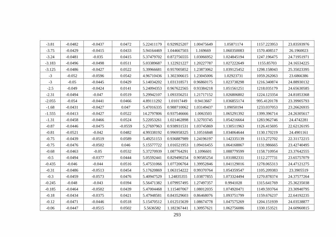
293

-3.81 -0.0482 -0.0437 0.0472 5.22411179 0.929925207 1.00475649 1.05871174 1157.223953 23.83593976

-3.75 -0.0429 -0.0415 0.0433 5.94164469 1.044667503 1.169669 1.060350083 1570.408517 26.1960023

-3.24 -0.0481 -0.035 0.0415 5.37479702 0.872756555 1.03066952 1.024845194 1247.196475 24.71951971

-3.183 -0.0496 -0.0498 0.0511 5.03389687 1.122921227 1.20227787 1.027222649 1155.85703 24.16534225

-3.125 -0.0486 -0.0427 0.0522 5.39966681 0.957005852 1.23873062 1.039125452 1298.158043 25.35023395

-3 -0.052 -0.0596 0.0542 4.96710436 1.302306615 1.23045006 1.02923731 1059.262063 23.6866386

-3 -0.05 -0.0445 0.0429 5.14034202 1.031318571 0.96860175 1.023738298 1216.340874 24.88930132

-2.5 -0.049 -0.0424 0.0141 5.24094353 0.967622565 0.93384218 1.051561251 1218.035179 24.65630585

-2.31 -0.0494 -0.047 0.0519 5.29942107 1.093356251 1.21717152 1.026806802 1224.123354 24.81853368

-2.055 -0.054 -0.0441 0.0466 4.89111292 1.01017449 0.9413667 1.036855174 995.4120178 23.39905793

-1.68 -0.0431 -0.0427 0.047 5.47016335 0.988710062 1.03149437 1.09050194 1233.037053 23.26626935

-1.555 -0.0413 -0.0427 0.0522 14.2797806 0.937546666 1.0063503 1.065291392 1399.396714 24.26305617

-1.31 -0.0458 -0.0466 0.0524 5.22053261 1.021462898 1.32703745 1.054216664 1283.962746 24.4742281

-0.87 -0.0446 -0.0475 -0.0559 5.27697963 0.938931531 1.03745869 1.130511963 1126.415695 22.62126195

-0.81 -0.0521 -0.042 0.0482 4.99338192 0.996958325 1.10516848 1.034064644 1130.170219 24.4901161

-0.75 -0.0439 -0.0519 0.0589 5.49251153 0.936887989 1.24196197 1.142335139 1113.272702 22.31172215

-0.75 -0.0476 -0.0502 0.046 5.15577722 1.016521953 1.09416455 1.064168867 1131.986665 23.42740495

-0.68 -0.0463 -0.05 0.0532 5.37270939 1.087764291 1.1096601 1.088779599 1158.710954 23.37642555

-0.5 -0.0494 -0.0377 0.0444 5.05592441 0.829490254 0.90585254 1.031882331 1112.277731 23.65757079

-0.435 -0.046 -0.044 0.0516 5.47531066 1.077206764 1.39952846 1.041129016 1278.065313 24.47121275

-0.31 -0.0486 -0.0513 0.0454 5.17620869 1.063154222 0.99370764 1.054359547 1105.209383 23.3905519

-0.3 -0.0459 -0.0573 0.0476 5.40947529 1.24835355 1.03877855 1.073324494 1270.878374 24.37577264

-0.245 -0.048 -0.043 0.0394 5.56471382 1.079957495 1.27497357 0.9941028 1315.641769 25.36235038

-0.185 -0.0464 -0.0502 0.0439 5.47004468 1.115407067 1.08012035 1.074920471 1149.593764 23.30940795

-0.18 -0.0434 -0.0375 0.0421 5.47948581 0.843529603 0.86468076 1.093751799 1159.676237 22.64192235

-0.12 -0.0471 -0.0446 0.0518 5.15470512 1.012515639 1.08674778 1.047575269 1204.151939 24.03538877

-0.06 -0.0447 -0.0515 0.0502 5.5636582 1.182367441 1.30957621 1.062756086 1330.153521 24.60960815

294

-0.06 -0.046 -0.0482 0.0598 5.2445295 1.023535033 1.25568999 1.065905224 1156.638316 23.2797202

-0.005 -0.0412 -0.049 0.0467 6.10793537 1.310563825 1.26404077 1.093736684 1530.703886 25.34511425

0 -0.0455 -0.0478 0.0471 5.50597051 1.042149485 1.20763794 1.065543842 1176.100707 23.3468346

0 -0.0449 -0.045 0.0503 5.4529455 1.189438817 1.11581298 1.131098446 1193.487529 23.36319135

0.12 -0.047 -0.0417 0.0522 5.31511265 0.979877688 1.11626975 1.064144639 1283.479172 24.78810885

0.173 -0.0461 -0.0443 0.0466 5.29837196 0.963357862 0.98282938 1.062945341 1240.533087 24.1354106

0.19 -0.0499 -0.0451 0.0487 4.87899252 0.932178822 0.9101128 1.09442434 966.5020201 22.16418205

0.19 -0.0455 -0.0519 0.0504 5.50396346 1.22283934 1.28578146 1.045468547 1366.758773 25.16817275

0.245 -0.0494 -0.0427 0.0442 5.25204199 0.9655268 1.04528461 1.022307869 1188.181165 24.45146355

0.25 -0.0471 -0.0447 0.0461 5.54933391 1.020225875 1.22046515 1.052093336 1237.133086 24.36232415

0.37 -0.0483 -0.045 0.0517 5.40473704 0.904295486 1.12387466 1.077142774 1107.849542 23.34608215

0.435 -0.048 -0.0558 0.05 5.24042761 1.15882397 1.12518796 1.085908658 1025.679285 22.39373135

0.5 -0.0473 -0.047 0.0422 5.37323364 1.073361534 1.10777787 1.031168536 1163.206635 23.673314

0.5 -0.0452 -0.045 0.0526 5.30917139 1.106485902 1.095527 1.096272002 1220.359554 23.70353795

0.56 -0.0439 -0.0469 0.0501 5.45200452 1.006250486 1.08657265 1.106616375 1145.340574 22.6307859

1.185 -0.0598 -0.0425 0.0438 4.76374495 1.004203719 0.99580024 0.992113334 969.2596012 24.29800968

1.495 -0.0455 -0.0532 0.0461 5.00780608 1.093610024 0.83017839 1.13333312 978.4695863 21.2950869

1.56 -0.0496 -0.0474 0.0494 5.22898951 1.140776683 1.3009019 0.987025768 1209.300776 24.7177

2.685 -0.0416 -0.0616 0.0509 5.52727408 1.168633619 1.19068698 1.146625162 1197.340569 22.52452115

3.25 -0.0494 -0.0534 0.0565 5.03976122 1.101614713 1.24309265 1.045705066 1035.324006 22.82452085

3.815 -0.046 -0.0578 0.0453 5.27852176 1.055330353 0.93054266 1.173954461 970.1950775 21.32104575

4.375 -0.0543 -0.0523 0.0455 4.60154662 0.971574715 0.98767844 1.006660868 838.3781728 21.533764

9.5 -0.0533 -0.0572 0.0594 4.31831615 0.941873364 0.92525626 1.089000562 771.2391105 20.46247585

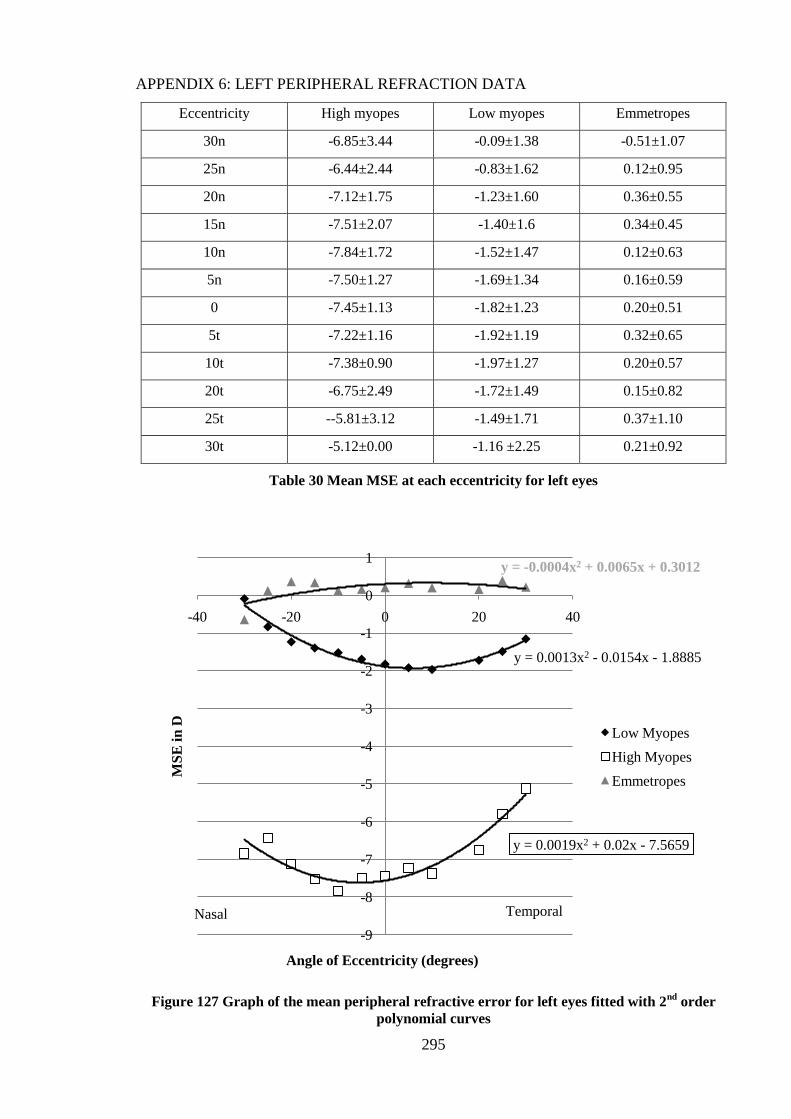
295

APPENDIX 6: LEFT PERIPHERAL REFRACTION DATA


30n -6.85±3.44 -0.09±1.38 -0.51±1.07

25n -6.44±2.44 -0.83±1.62 0.12±0.95

20n -7.12±1.75 -1.23±1.60 0.36±0.55

15n -7.51±2.07 -1.40±1.6 0.34±0.45

10n -7.84±1.72 -1.52±1.47 0.12±0.63

5n -7.50±1.27 -1.69±1.34 0.16±0.59

0 -7.45±1.13 -1.82±1.23 0.20±0.51

5t -7.22±1.16 -1.92±1.19 0.32±0.65

10t -7.38±0.90 -1.97±1.27 0.20±0.57

20t -6.75±2.49 -1.72±1.49 0.15±0.82

25t --5.81±3.12 -1.49±1.71 0.37±1.10

30t -5.12±0.00 -1.16 ±2.25 0.21±0.92

Table 30 Mean MSE at each eccentricity for left eyes

Figure 127 Graph of the mean peripheral refractive error for left eyes fitted with 2nd

order

polynomial curves

y = 0.0013x2 - 0.0154x - 1.8885

y = 0.0019x2 + 0.02x - 7.5659

y = -0.0004x2 + 0.0065x + 0.3012

-9

-8

-7

-6

-5

-4

-3

-2

-1

0

1

-40 -20 0 20 40

MS

E i

n D

Angle of Eccentricity (degrees)

Low Myopes

High Myopes

Emmetropes

Nasal Temporal

296


30n 0.75±2.30 1.21±1.18 -0.82±1.25

25n 1.11±1.58 0.99±1.30 -0.07±1.20

20n 0.43±1.02 0.59±1.05 0.16±0.62

15n -0.07±1.27 0.43±0.92 0.13±0.46

10n -0.40±0.89 0.30±0.64 -0.08±0.57

5n -0.05±0.35 0.13±0.47 -0.04±0.34

5t 0.23±0.19 -0.10±0.34 0.01±0.33

10t 0.07±0.33 -0.14±0.59 0.00±0.23

20t 0.81±1.86 0.10±1.21 -0.05±0.78

25t 1.74±2.46 0.36±1.98 0.21±1.15

30t 3.56±0.00 1.72±0.30 -0.06±0.57

Table 31 Mean difference in MSE values between central and peripheral locations, data is

shown for left eyes

Figure 128 Graphical representation of the mean difference in MSE between the central and

peripheral locations, left eyes

y = 0.0015x2 - 0.0042x - 0.0825

y = 0.0025x2 + 0.0278x - 0.1924

y = -0.0004x2 + 0.0058x + 0.1009

-2

-1

0

1

2

3

4

5

-40 -30 -20 -10 0 10 20 30 40

Dif

fere

nce

bet

wee

nce

ntr

al

an

d p

erip

her

al

mea

n

MS

E (

in D

)


Low Myopes

High Myopes

Emmetropes

Nasal Temporal

297

Eccentricity High myopes Emmetropes Low myopes

30n 0.38±0.19 -1.07±0.74 0.01±0.94

25n 0.32±0.48 -0.43±0.69 0.12±0.81

20n 0.28±0.34 -0.24±0.42 0.22±0.70

15n 0.35±0.60 -0.08±0.38 0.38±0.47

10n 0.53±0.39 -0.06±0.30 0.30±0.44

5n 0.13±0.31 0.02±0.28 0.30±0.43

0 -0.07±0.30 0.01±0.24 0.22±0.43

5t 0.02±0.59 -0.06±0.26 0.16±0.55

10t -0.19±0.94 -0.07±0.34 -0.04±0.59

20t -0.11±0.76 -0.56±0.57 -0.28±0.84

25t 0.12±1.05 -0.63±0.85 -0.51±1.08

30t -0.23±0.00 -0.81±0.54 -0.14±0.84

Table 32 Mean J180 values left eye based on eccentricity

Figure 129 Mean J180 values for left eyes, fitted with 2nd

order polynomial curves

y = -0.0004x2 - 0.009x + 0.1997

y = -3E-05x2 - 0.0088x + 0.1606

y = -0.0011x2 - 0.0014x + 0.0313

-1.2

-1

-0.8

-0.6

-0.4

-0.2

0

0.2

0.4

0.6

0.8

-40 -30 -20 -10 0 10 20 30 40

J180 i

n D


Low Myopes

High Myopes

Emmetropes

Nasal Temporal

298


30n -0.10±0.46 0.14±0.19 0.22±0.46

25n 0.04±0.30 0.13±0.31 0.16±0.31

20n -0.06±0.35 0.10±0.29 0.23±0.29

15n -0.33±-0.54 0.00±0.25 0.07±0.27

10n -0.06±0.40 0.03±0.26 0.17±0.28

5n -0.32±0.34 -0.02±0.27 0.12±0.15

0 -0.24±0.36 0.14±0.38 0.05±0.14

5t -0.26±0.23 0.07±0.38 0.06±0.17

10t -0.15±0.31 0.05±0.42 -0.04±0.26

20t -0.20±0.33 -0.03±0.48 0.03±0.47

25t -0.04±0.73 -0.14±0.62 0.05±0.48

30t -0.09±0.00 -0.07±0.71 0.63±0.34

Table 33 J45 left eye, based on eccentricity

Figure 130 Mean J45 values for left eyes, fitted with linear trend lines

y = -0.0035x + 0.0305

y = -0.003x - 0.1891

y = 0.001x + 0.146

-0.60

-0.40

-0.20

0.00

0.20

0.40

0.60

0.80

-40 -30 -20 -10 0 10 20 30 40

J4

5 i

n D


Low Myopes

High Myopes

Emmetropes

Nasal Temporal

299


30n -1.12±0.22 -1.51±0.91 -2.46±1.29

25n -1.02±0.69 -1.56±0.74 -1.50±0.91

20n -0.96±0.51 -1.35±0.77 -1.05±0.58

15n -1.46±1.09 -1.14±0.58 -0.76±0.57

10n -1.34±0.69 -0.93±0.72 -0.74±0.49

5n -0.93±0.65 -0.91±0.70 -0.57±0.37

0 -0.78±0.67 -0.98±0.76 -0.48±0.30

5t -1.02±0.83 -1.15±0.68 -0.55±0.31

10t -1.37±1.41 -1.21±0.73 -0.77±0.40

20t -1.46±0.69 -1.72±0.94 -1.70±0.68

25t -2.22±1.16 -2.25±1.40 -2.14±0.98

30t -0.50±0.00 -1.56±0.44 -2.25±0.74

Table 34 Cylindrical component calculated from vector components J180 and J45. Left eye data

is shown

Table 35 Graphical representation of the cylindrical component, left eyes only

-3.00

-2.50

-2.00

-1.50

-1.00

-0.50

0.00

-40 -30 -20 -10 0 10 20 30 40

Cyli

nd

rica

l co

mp

on

ent

(in

D)


Low Myopes

High Myopes

Emmetropes

300

APPENDIX 7: RIGHT PERIPHERAL REFRACTION AND RETFIT DATA

Raw RE refraction data and values for sagittal refraction and interval of sturm as described

in section 11.6

N N N N N N N T T T T T

tang

K

Eccentricity -30 -25 -20 -15 -10 -5 0 5 10 20 25 30 8.04

Sph 0.37 0.12 -0.5 -0.5 -0.8 -0.1 -0.4 -0.8 -0.9 -0.6 -0.1 -0.9

Cyl -3 -2.4 -1.5 -1.1 -0.9 -0.4 -0.6 -0.9 -0.5 -0.5 -1.6 -0.4

Axis 108 106 112 110 137 134 111 51 117 120 69 132

Int sturm 3 2.37 1.5 1.12 -0.9 0.37 0.62 0.87 0.5 0.5 1.62 0.37

sag 0.37 0.12 -0.5 -0.5 -1.6 -0.1 -0.4 -0.8 -0.9 -0.6 -0.1 -0.9

Eccentricity -30 -25 -20 -15 -10 -5 0 5 10 20 25 30 7.76

Sph

1.62 0.62 0.25 0.12 -0.3 -0.3 -0.3 0.37 1.75 2.12

Cyl

-1.6 -1.3 -0.9 -1 -0.5 -0.5 -0.3 -0.9 -1.3 -1.5

Axis

136 120 116 140 120 114 56 68 48 48

Int sturm -1.6 1.25 0.87 -1 0.5 0.5 0.25 0.87 1.25 1.5

sag

0 0.62 0.25 -0.9 -0.3 -0.3 -0.3 0.37 1.75 2.12

Eccentricity -30 -25 -20 -15 -10 -5 0 5 10 20 25 30 7.65

Sph 5.87 5.87 6.12 5 5.12 4.87 4.75 4.37 4.25 4.62 5.37

Cyl -1.4 -1.6 -1.8 -1.3 -1.1 -1.3 -0.8 -0.4 -0.6 -1.1 -1

Axis 109 109 111 102 109 109 113 123 116 82 81

Int sturm 1.37 1.62 1.75 1.25 1.12 1.25 0.75 0.37 0.62 1.12 1

Sag 5.87 5.87 6.12 5 5.12 4.87 4.75 4.37 4.25 4.62 5.37

Eccentricity -30 -25 -20 -15 -10 -5 0 5 10 20 25 30 7.67

Sph -0.6 0.12 0.25 0.62 0.5 0.5 1.12 0.87 0.25 1.5 1.62

Cyl -2 -1.6 -1.6 -2.3 -0.6 -0.8 -1.1 -1.3 -0.6 -3.3 -3.3

Axis 104 89 100 119 87 99 101 100 94 87 82

Int sturm 2 1.62 1.62 2.25 0.62 0.75 1.12 1.25 0.62 3.25 3.25

sag -0.6 0.12 0.25 0.62 0.5 0.5 1.12 0.87 0.25 1.5 1.62

Eccentricity -30 -25 -20 -15 -10 -5 0 5 10 20 25 30 7.79

Sph 2.75 3.37 2.25 1.12 1.25 0.87 -0.3 -1.1 -1.9 2.37

Cyl -1.8 -2.1 -1.5 -1.4 -1.8 -1.1 -1 -0.5 -1.4 -4.9

Axis 4 175 13 15 12 7 34 49 83 81

Int sturm -1.8 -2.1 -1.5 -1.4 -1.8 -1.1 -1 0.5 1.37 4.87

sag 1 1.25 0.75 -0.3 -0.5 -0.3 -1.3 -1.1 -1.9 2.37

Eccentricity -30 -25 -20 -15 -10 -5 0 5 10 20 25 30 7.71

Sph

-3.6 -7.8 -8.1 -8.8 -8.1 -7.9 -8.6 -7.9 -7.6 -6.6

Cyl

-4.1 -1.3 -1.8 -0.6 -1.1 -1 -1.1 -0.9 -1.5 -1.8

Axis

163 176 162 180 172 150 139 130 117 125

Int sturm -4.1 -1.3 -1.8 -0.6 -1.1 -1 -1.1 0.87 1.5 1.75

301

sag

-7.7 -9 -9.9 -9.4 -9.2 -8.9 -9.7 -7.9 -7.6 -6.6

Eccentricity -30 -25 -20 -15 -10 -5 0 5 10 20 25 30 7.57

sph -2 -3.1 -3.8 -5 -4.9 -5.5 -4.4 -5.3 -5.6 -4.6 -4 0.5

Cyl -3.1 -2.6 -2.6 -1.5 -1.4 -0.9 -0.8 -0.8 -0.5 -2 -0.9

Axis 172 180 3 6 154 168 170 171 131 93 155

Int sturm -3.1 -2.6 -2.6 -1.5 -1.4 -0.9 -0.8 -0.8 0.5 2 -0.9

sag -5.1 -5.7 -6.4 -6.5 -6.2 -6.4 -5.1 -6 -5.6 -4.6 -4.9

Eccentricity -30 -25 -20 -15 -10 -5 0 5 10 20 25 30 8.11

1.12 0.75 -0.3 -0.1 0 0.25 0.87 0.38 -0.3 0.62 0.5

Cyl

-1.9 -1.4 -0.5 -0.5 -0.5 -1.1 -1.3 -1.3 -1.3 -1.8

Axis

103 89 57 115 92 81 74 89 93 94

Int sturm 1.87 1.37 0.5 0.5 0.5 1.12 1.25 1.25 1.25 1.75

sag

1.12 0.75 -0.3 -0.1 0 0.25 0.87 0.38 -0.3 0.62

Eccentricity -30 -25 -20 -15 -10 -5 0 5 10 20 25 30 8.26

Sph

-6.8 -6.6 -6.8 -6.9 -6.6 -6.1 -5.1

Cyl

-0.5 -0.8 -0.8 -0.9 -0.9 -0.8 -1.9

Axis

25 65 95 5 11 13 89

Int sturm

-0.5 0.75 0.75 -0.9 -0.9 -0.8 1.87

sag

-7.3 -6.6 -6.8 -7.7 -7.5 -6.9 -5.1

Eccentricity -30 -25 -20 -15 -10 -5 0 5 10 20 25 30 7.62

Sph -7.3 -7.9 -8 -8.5 -8 -8.3 -8.9 -8 -7.8 -6.4 -5.9

Cyl -0.5 -0.5 -0.9 -0.5 -0.8 -0.4 -0.5 -1 -2 -2.4 -0.9

Axis 142 144 143 159 14 163 111 82 75 60 74

Int sturm -0.5 -0.5 -0.9 -0.5 -0.8 -0.4 0.5 1 2 2.37 0.87

sag -7.8 -8.4 -8.9 -9 -8.8 -8.6 -8.9 -8 -7.8 -6.4 -5.9

Eccentricity -30 -25 -20 -15 -10 -5 0 5 10 20 25 30 7.69

Sph 1.12 0.75 0.12 -0.5 0 -0.1 -0.3 -0.1 -0.6 -1.4 0.5

Cyl -1.3 -0.9 -0.8 -0.4 -0.5 -0.5 -0.1 -1.1 -0.5 -0.6 -0.8

Axis 117 113 120 27 167 21 13 17 59 59 28

Int sturm 1.25 0.87 0.75 -0.4 -0.5 -0.5 -0.1 -1.1 0.5 0.62 -0.8

sag 1.12 0.75 0.12 -0.9 -0.5 -0.6 -0.4 -1.2 -0.6 -1.4 -0.3

Eccentricity -30 -25 -20 -15 -10 -5 0 5 10 20 25 30 7.8

Sph 2.87 1.37 1.25 1 0.62 0.5 0.5 0.75 1 2.5

Cyl -2.3 -1.3 -1.5 -1.4 -0.5 -0.4 -0.3 -0.4 -0.8 -0.8

Axis 171 167 150 164 164 135 51 82 66 2

Int sturm -2.3 -1.3 -1.5 -1.4 -0.5 0.37 0.25 0.37 0.75 -0.8

Sag 0.62 0.12 -0.3 -0.4 0.12 0.5 0.5 0.75 1 1.75

Eccentricity -30 -25 -20 -15 -10 -5 0 5 10 20 25 30 7.78

Sph 1.75 1.25 0.75 0.12 0 0 0 0.12 0.25 0 0.75

Cyl -0.9 -0.4 -1.6 -0.5

-0.1 -0.1

-0.3

-0.6

Axis 85 75 114 65

128 55

71

100

302

Int sturm 0.87 0.37 1.62 0.5 0 0.12 0.12 0 0.25 0 0.62

Sag 1.75 1.25 0.75 0.12 0 0 0 0.12 0.25 0 0.75

Eccentricity -30 -25 -20 -15 -10 -5 0 5 10 20 25 30 7.66

Sph ` -5.4 -6 -5.8 -5.5 -5.1 -5.4 -5.1 -4.9 -4.5

Cyl

-0.4 -0.6 -2.3 -1.1 -1.3 -0.4 -0.6 -0.5 -1

Axis

174 166 175 174 154 97 110 95 100

Int sturm -0.4 -0.6 -2.3 0 -1.3 0.37 0.62 0.5 1

Sag

-5.7 -6.6 -8 -6.6 -6.4 -5.4 -5.1 -4.9 -4.5

Eccentricity -30 -25 -20 -15 -10 -5 0 5 10 20 25 30 7.8

Sph ` 2.25 1.25 0.75 0.25 0 0.12 0.12 0.5 0.87 1.62

Cyl

-1.4 -0.6 -0.4 -1.3 -0.1 -0.3 -0.3 -0.6 -1.3 -2

Axis

90 108 107 36 151 143 46 95 85 73

Int sturm 1.37 0.62 0.37 -1.3 -0.1 -0.3 0.25 0.62 1.25 2

Sag

2.25 1.25 0.75 -1 -0.1 -0.1 0.12 0.5 0.87 1.62

Eccentricity -30 -25 -20 -15 -10 -5 0 5 10 20 25 30 8.14

Sph 1.62 1.5 1.62 0.37 0.75 0.25 0.12 0.5 0.87 1.62 2.25

Cyl

-0.4 -0.5 -1 -1 -0.4 -0.3 -0.1 -0.5 -1.1 -1.1

Axis

5 172 22 21 33 171 30 10 175 33

Int sturm 0 -0.4 -0.5 -1 -1 -0.4 -0.3 -0.1 -0.5 -1.1 -1.1

Sag 1.62 1.13 1.12 -0.6 -0.3 -0.1 -0.1 0.38 0.37 0.5 1.13

Eccentricity -30 -25 -20 -15 -10 -5 0 5 10 20 25 30 7.88

Sph -0.6 0.25 0.12 0.12 0.37 0 0.25 0.25 0.12 -0.5 -0.3

Cyl -2.1 -1.1 -0.9 -1.1 -0.8 -0.6 -0.9 -0.8 -1.3 -2.8 -1.8

Axis 104 83 117 123 118 119 98 95 70 82 83

Int sturm 2.12 1.12 0.87 1.12 0.75 0.62 0.87 0.75 1.25 2.75 1.75

Sag -0.6 0.25 0.12 0.12 0.37 0 0.25 0.25 0.12 -0.5 -0.3

Eccentricity -30 -25 -20 -15 -10 -5 0 5 10 20 25 30 7.9

Sph 2.75 1.12 -0.1 -0.6 -1.1 -2.3 -2.8 -2.4 -2.6 -2.6 -2 -1.1

Cyl -2.8 -1.6 -0.9 -1.9 -1.8 -0.8 -0.3 -0.6 -0.6 -0.5 -0.4 -0.8

Axis 17 24 31 43 161 30 103 96 141 77 140 159

Int sturm -2.8 -1.6 -0.9 -1.9 -1.8 -0.8 0.25 0.62 -0.6 0.5 -0.4 -0.8

Sag 0 -0.5 -1 -2.5 -2.9 -3 -2.8 -2.4 -3.2 -2.6 -2.4 -1.9

Eccentricity -30 -25 -20 -15 -10 -5 0 5 10 20 25 30 7.98

Sph 1.25 1.37 1.12 1 0.75 0.5 0.75 0.12 0.12 0.12 0

Cyl -2.5 -1.1 -0.4 -0.8 -0.1 -0.1 -0.5 -0.1 -0.5 -2.4 -2.8

Axis 74 77 51 37 13 159 17 20 70 88 90

Int sturm 2.5 1.12 0.37 -0.8 -0.1 -0.1 -0.5 -0.1 0.5 2.37 2.75

Sag 1.25 1.37 1.12 0.25 0.63 0.38 0.25 0 0.12 0.12 0

Eccentricity -30 -25 -20 -15 -10 -5 0 5 10 20 25 30 8.42

Sph

-0.8 0.75 0.12 0.12 0.12 -0.3 0 0.25 0.87

Cyl

-3.1 -1.1 -0.4 -0.1 -0.3 -0.1 -0.6 -1.5 -3.6

303

Axis

93 98 91 151 52 106 90 82 73

Int sturm 3.12 1.12 0.37 -0.1 0.25 0.12 0.62 1.5 3.62

Sag

-0.8 0.75 0.12

0.12 -0.3 0 0.25 0.87

Eccentricity -30 -25 -20 -15 -10 -5 0 5 10 20 25 30 7.51

Sph 0.25 0.37 0 -0.5 0 0 -0.3 0 0.25 0.25 0.37

Cyl -1.1 -1.3 -0.6 -0.4 -0.6 -0.6 -0.4 -0.8 -1.9 -2.9 -2.5

Axis 89 98 77 165 99 88 90 70 80 90 86

Int sturm 1.12 1.25 0.62 -0.4 0.62 0.62 0.37 0.75 1.87 2.87 2.5

Sag 0.25 0.37 0 -0.9

0 -0.3 0 0.25 0.25 0.37

Eccentricity -30 -25 -20 -15 -10 -5 0 5 10 20 25 30 7.23

sph -1.3 -3.6 -6.4 -6.6 -7.5 -7.5 -7.9 -7.6 -7.4 -5.5 -1 -1.5

Cyl -2.6 -1.6 -0.6 -1.1 -1 -0.6 -1 -1.4 -1.3 -0.5 -2 -2

Axis 177 178 132 137 134 114 97 92 93 23 176 1

Int sturm -2.6 -1.6 0.62 -1.1 1 0.62 1 1.37 1.25 -0.5 -2 -2

Sag -3.9 -5.2 -6.4 -7.7 -7.5 -7.5 -7.9 -7.6 -7.4 -6 -3 -3.5

Eccentricity -30 -25 -20 -15 -10 -5 0 5 10 20 25 30 7.87

Sph

0.12 0.12 0.37 0.62 0.12 0 0.12 -0.1 0.12 0.5 0.37

Cyl

-2.8 -3 -1.9 -1 -0.4 -0.1 -0.5 -0.8 -1.8 -1.6 -2.3

Axis

75 76 77 75 72 76 116 122 96 111 112

Int sturm 2.75 3 1.87 1 0.37 0.12 0.5 0.75 1.75 1.62 2.25

Sag

0.12 0.12 0.37 0.62 0.12

0.12 -0.1 0.12 0.5 0.37

Eccentricity -30 -25 -20 -15 -10 -5 0 5 10 20 25 30 8.19

Sph -10 -11 -11 -11 -10 -11 -9.8 -9.9 -9.6 -9.5 -6.6

Cyl -1.8 -1.3 -2.4 -2.9 -1.8 -1.3 -1.6 -1.4 -3.4 -1.8 -4

Axis 13 46 49 47 48 35 51 46 48 54 24

Int sturm -1.8 1.25 2.37 2.87 1.75 -1.3 1.62 1.37 3.37 1.75 -4

Sag -12 -11 -11 -11 -10 -12 -9.8 -9.9 -9.6 -9.5 -11

Eccentricity -30 -25 -20 -15 -10 -5 0 5 10 20 25 30 7.65

sph

-1.6 -1.8 -1.8 -2 -2.5 -2.4 -1.8

Cyl

-3.9 -2.9 -3 -2.3 -2.3 -1.9 -3.5

Axis

180 5 5 5 28 8 19

Int sturm -3.9 -2.9 -3 -2.3 -2.3 -1.9 -3.5

Sag

-5.5 -4.6 -4.8 -4.3 -4.8 -4.2 -5.3

Eccentricity -30 -25 -20 -15 -10 -5 0 5 10 20 25 30 7.69

Sph -1.9 -1.9 -2.1 -2.6 -2.6 -2.9 -2.5 -2.4 -2.3 -1.6 -1

Cyl -3.3 -3.3 -3.1 -0.8 -1 -0.4 -0.4 -0.5 -0.6 -1.8 -3.1

Axis 97 100 90 80 86 112 157 123 122 90 90

Int sturm 3.25 3.25 3.12 0.75 1 0.37 -0.4 0.5 0.62 1.75 3.12

Sag -1.9 -1.9 -2.1 -2.6 -2.6 -2.9 -2.9 -2.4 -2.3 -1.6 -1

Eccentricity -30 -25 -20 -15 -10 -5 0 5 10 20 25 30 7.63

Sph 1.62 1 0.25 -0.9 -1.6 -1.9 -2.3 -1.9 -1.8 -0.6 0.12 1

304

Cyl -5.6 -4 -1.9 -1.4 -0.8 -0.8 -0.1 -0.8 -1 -1.1 -1.4 -1.5

Axis 90 83 72 71 65 36 12 179 7 172 168 171

Int sturm 5.62 4 1.87 1.37 0.75 -0.8 -0.1 -0.8 -1 -1.1 -1.4 -1.5

Sag 1.62 1 0.25 -0.9 -1.6 -2.6 -2.4 -2.6 -2.8 -1.7 -1.3 -0.5

Eccentricity -30 -25 -20 -15 -10 -5 0 5 10 20 25 30 7.64

Sph 2.37 1.25 0.87 0 0.25 0.13 -0.1 -0.8 -1 -1.9 -1.9 -1.8

Cyl -4.3 -3.1 -2.6 -1.6 -2 -1.8 -1.4 -1 -1.1 -2 -2.1 -2

Axis 2 178 177 175 4 5 14 23 36 71 64 71

Int sturm -4.3 -3.1 -2.6 -1.6 -2 -1.8 -1.4 -1 -1.1 2 2.12 2

Sag -1.9 -1.9 -1.8 -1.6 -1.8 -1.6 -1.5 -1.8 -2.1 -1.9 -1.9 -1.8

Eccentricity -30 -25 -20 -15 -10 -5 0 5 10 20 25 30 7.64

Sph -0.1 -1.3 -1.8 -2.1 -2.4 -2 -1.6 -1.4 -1.3 -0.6 0.25 1.25

Cyl -1.4 -1.4 -1 -1.1 -2 -1.1 -0.6 -0.8 -0.6 -0.9 -1.9 -1.8

Axis 131 149 148 163 167 11 155 148 113 105 98 102

Int sturm 1.37 -1.4 -1 -1.1 -2 -1.1 -0.6 -0.8 0.62 0.87 1.87 1.75

Sag -0.1 -2.6 -2.8 -3.2 -4.4 -3.1 -2.2 -2.1 -1.3 -0.6 0.25 1.25

Eccentricity -30 -25 -20 -15 -10 -5 0 5 10 20 25 30 7.91

Sph `

1.37 0.87 0.12 0.25 0.62 0.62 0.87 0.87

Cyl

-0.8 -0.8 -0.4 -0.6 -0.8 -0.9 -1 -1.8

Axis

50 88 59 83 87 96 99 105

Int sturm

0.75 0.75 0.37 0.62 0.75 0.87 1 1.75

Sag

1.37 0.87 0.12 0.25 0.62 0.62 0.87 0.87

Eccentricity -30 -25 -20 -15 -10 -5 0 5 10 20 25 30 8.06

Sph 1.87 2.37 1.62 1.12 0.87 0.75 0.75 0.37 0.62 1.25 1.37

Cyl -1.3 -0.6 -0.5 -0.9 -0.4 -0.4 -0.5 -0.4 -0.5 -2.4 -3.6

Axis 62 59 165 174 47 69 180 53 95 88 91

Int sturm 1.25 0.62 -0.5 -0.9 0.37 0.37 -0.5 0.37 0.5 2.37 3.62

Sag 1.87 2.37 1.12 0.25 0.87 0.75 0.25 0.37 0.62 1.25 1.37

Eccentricity -30 -25 -20 -15 -10 -5 0 5 10 20 25 30 7.88

Sph ` 0.37 1.37 1.62 2 2.37 1.62 1.37 1.12 1.12 1.5

Cyl

-1.8 -0.3 -0.3 -0.8 -0.4 -0.3 -0.4 -0.3 -2.1 -0.9

Axis

77 47 14 169 179 7 19 72 89 90

Int sturm 1.75 0.25 -0.3 -0.8 -0.4 -0.3 -0.4 0.25 2.12 0.87

Sag

0.37 1.37 1.37 1.25 2 1.37 1 1.12 1.12 1.5

Eccentricity -30 -25 -20 -15 -10 -5 0 5 10 20 25 30 7.7

Sph

-0.5 -0.6 -1.3 -0.6 -0.6 -0.1 -0.3 -0.1 0.13

Cyl

-1.8 -1.3 -1 -0.3 -0.5 -0.4 -0.4 -0.6 -1.1

Axis

97 112 125 147 132 155 120 89 87

Int sturm

1.75 1.25 1 -0.3 0.5 -0.4 0.37 0.62 1.12

Sag

-0.5 -0.6 -1.3 -0.9 -0.6 -0.5 -0.3 -0.1 0.13

Eccentricity -30 -25 -20 -15 -10 -5 0 5 10 20 25 30 7.93

305

Sph -1.3 -1.9 -2.6 -2.9 -2.5 -2.9 -2.5 -2.6 -2.4 -3 -2.9

Cyl -2.5 -1.1 -0.5

-0.6 -1.3 -0.8 -0.5 -1.5 -4.6 -4.6

Axis 70 67 59

176 176 175 98 96 97 99

Int sturm 2.5 1.12 0.5 0 -0.6 -1.3 -0.8 0.5 1.5 4.62 4.62

Sag -1.3 -1.9 -2.6 -2.9 -3.1 -4.1 -3.3 -2.6 -2.4 -3 -2.9

Eccentricity -30 -25 -20 -15 -10 -5 0 5 10 20 25 30 7.94

Sph 0.5 0.87 1 1 1.12 0.87 1.37 1.37 1.5 1.75 1.5

Cyl -4.5 -1.8 -1.4 -0.9 -0.5 -0.4 -0.4 -0.5 -0.8 -2.4 -2.9

Axis 98 113 102 99 104 119 83 99 83 77 81

Int sturm 4.5 1.75 1.37 0.87 0.5 0.37 0.37 0.5 0.75 2.37 2.87

Sag 0.5 0.87 1 1 1.12 0.87 1.37 1.37 1.5 1.75 1.5

Eccentricity -30 -25 -20 -15 -10 -5 0 5 10 20 25 30 8.09

Sph 0.37 0.12 0.62 1 0.75 0.62 0.12 0.37 0.37 0.87 1.12

Cyl -3.1 -1.9 -1 -1.1 -0.3 -0.5 -0.4 -0.5 -0.5 -1.4 -2.1

Axis 97 104 133 136 92 131 103 58 63 73 83

Int sturm 3.12 1.87 1 -1.1 0.27 0.5 0.37 0.5 0.5 1.37 2.12

Sag 0.37 0.12 0.62 -0.1 0.75 0.62 0.12 0.37 0.37 0.87 1.12

Eccentricity -30 -25 -20 -15 -10 -5 0 5 10 20 25 30 7.7

Sph 1.62 2 2.12 2.87 2.25 2.12 1.87 2 1.75 1.87 2.25

Cyl -1.5 -1 -0.8 -0.4 -0.5 -0.3 -0.6 -0.8 -1.3 -2.5 -1.3

Axis 108 120 125 37 28 1 86 90 86 79 89

Int sturm 1.5 1 0.75 -0.4 -0.5 -0.3 0.62 0.75 1.25 2.5 1.25

Sag 1.62 2 2.12 2.5 1.75 1.87 1.87 2 1.75 1.87 2.25

Eccentricity -30 -25 -20 -15 -10 -5 0 5 10 20 25 30 8.06

Sph 0.87 0.87 0.75 -0.1 0.38 0.5 0.62 0.87 0.87 0.5 0.38

Cyl -3.8 -1.3 -1.1 -1.1 -0.9 -0.8 -0.4 -1 -1.1 -4.1 -5.4

Axis 100 117 118 136 116 112 83 78 77 87 82

Int sturm 3.75 1.25 1.12 -1.1 0.87 0.75 0.37 1 1.12 4.12 5.37

Sag 0.87 0.87 0.75 -1.2 0.38 0.5 0.62 0.87 0.87 0.5 0.38

Eccentricity -30 -25 -20 -15 -10 -5 0 5 10 20 25 30 7.53

Sph -0.6 -0.6 -0.8 -0.8 -0.4 -0.6 -0.8 -1.3 -0.8 -0.5 -0.1

Cyl -0.8 -0.8 -0.6 -1.3 -1.4 -1.6 -1.9 -1.9 -2.6 -3.4 -6.6

Axis 107 128 150 129 127 125 123 109 108 99 82

Int sturm 0.75 0.75 -0.6 1.25 1.37 1.62 1.87 1.87 2.62 3.37 6.62

Sag -0.6 -0.6 -1.4 -0.8 -0.4 -0.6 -0.8 -1.3 -0.8 -0.5 -0.1

Eccentricity -30 -25 -20 -15 -10 -5 0 5 10 20 25 30 8

Sph 0.75 0 0 -0.3 -0.3 -0.4 -0.1 -0.3 -0.1 0.12 0.25

Cyl -1.3 -0.8 -0.9 -0.9 -0.6 -0.3 -0.3 -0.3 -0.5 -1 -1

Axis 165 151 140 75 156 178 22 77 57 73 64

Int sturm -1.3 -0.8 -0.9 0.87 -0.6 -0.3 -0.3 0.25 0.5 1 1

Sag -0.5 -0.8 -0.9 -0.3 -0.9 -0.6 -0.4 -0.3 -0.1 0.12 0.25

306

Eccentricity -30 -25 -20 -15 -10 -5 0 5 10 20 25 30 7.51

Sph

0.87 0.12 0 0 0 0.12 0 0.25

Cyl

-0.8 -0.8 -0.9 -0.3 -0.1 -0.8 -0.4 -0.5

Axis

100 31 20 28 19 6 150 167

Int sturm 0.75 -0.8 -0.9 -0.3 -0.1 -0.8 -0.4 -0.5

Sag

0.87 -0.6 -0.9 -0.3 -0.1 -0.6 -0.4 -0.3

Eccentricity -30 -25 -20 -15 -10 -5 0 5 10 20 25 30 7.5

Sph -2.5 -4.1 -4.8 -5.1 -6.3 -6.8 -6.9 -6.1 -6 -4.4 -2.9 -2.4

Cyl -2.5 -2.3 -2.4 -1.8 -2.1

-0.4 -0.6 -1 -1 -2.5 -1.9

Axis 168 168 168 153 173

156 106 88 74 33 13

Int sturm -2.5 -2.3 -2.4 -1.8 -2.1 0 -0.4 0.62 1 1 -2.5 -1.9

Sag -5 -6.4 -7.1 -6.9 -8.4 -6.8 -7.2 -6.1 -6 -4.4 -5.4 -4.2

307

Apical radius (r) and conic constant values (p) derived through use of RetFit x and y^2

coordinates and SPSS statistical package v.16

SUBJECT b1 b2 Radius Conic

1 -24.461 -2.686 -12.2305 2.686

2 -27.879 -5.564 -13.9395 5.564

3 -21.984 -6.509 -10.992 6.509

4 -11.961 0.903 -5.9805 -0.903

5 -9.504 1.387 -4.752 -1.387

6 -10.677 5.592 -5.3385 -5.592

7 -19.175 -1.958 -9.5875 1.958

8 -14.166 -1.637 -7.083 1.637

9 -20.231 -2.067 -10.1155 2.067

10 -13.529 1.505 -6.7645 -1.505

11 -10.604 0.548 -5.302 -0.548

12 -25.786 -6.106 -12.893 6.106

13 -19.642 -2.717 -9.821 2.717

14 -33.08 -10.283 -16.54 10.283

15 0.476 2.196 0.238 -2.196

16 15.13 15.628 7.565 -15.628

17 -8.211 0.767 -4.1055 -0.767

18 5.479 5.55 2.7395 -5.55

19 -13.121 -0.31 -6.5605 0.31

20 -31.199 -7.731 -15.5995 7.731

21 -17.085 -0.228 -8.5425 0.228

22 -33.523 -11.291 -16.7615 11.291

23 -12.211 8.026 -6.1055 -8.026

24 -25.327 -3.81 -12.6635 3.81

25 -10.298 0.549 -5.149 -0.549

26 -13.855 1.439 -6.9275 -1.439

27 -36.535 -11.005 -18.2675 11.005

28 -22.672 -4.114 -11.336 4.114

29 -24.151 -3.47 -12.0755 3.47

30 -2.236 4.131 -1.118 -4.131

31 -8.017 3.761 -4.0085 -3.761

32 -22.38 -2.934 -11.19 2.934

33 -20.866 -2.496 -10.433 2.496

34 -24.557 -2.582 -12.2785 2.582

35 1.512 5.884 0.756 -5.884

36 -23.081 -0.83 -11.5405 0.83

37 -39.467 -8.658 -19.7335 8.658

38 -17.851 -0.919 -8.9255 0.919

39 -17.182 -1.188 -8.591 1.188

40 -21.84 -3.911 -10.92 3.911

41 -13.306 0.346 -6.653 -0.346

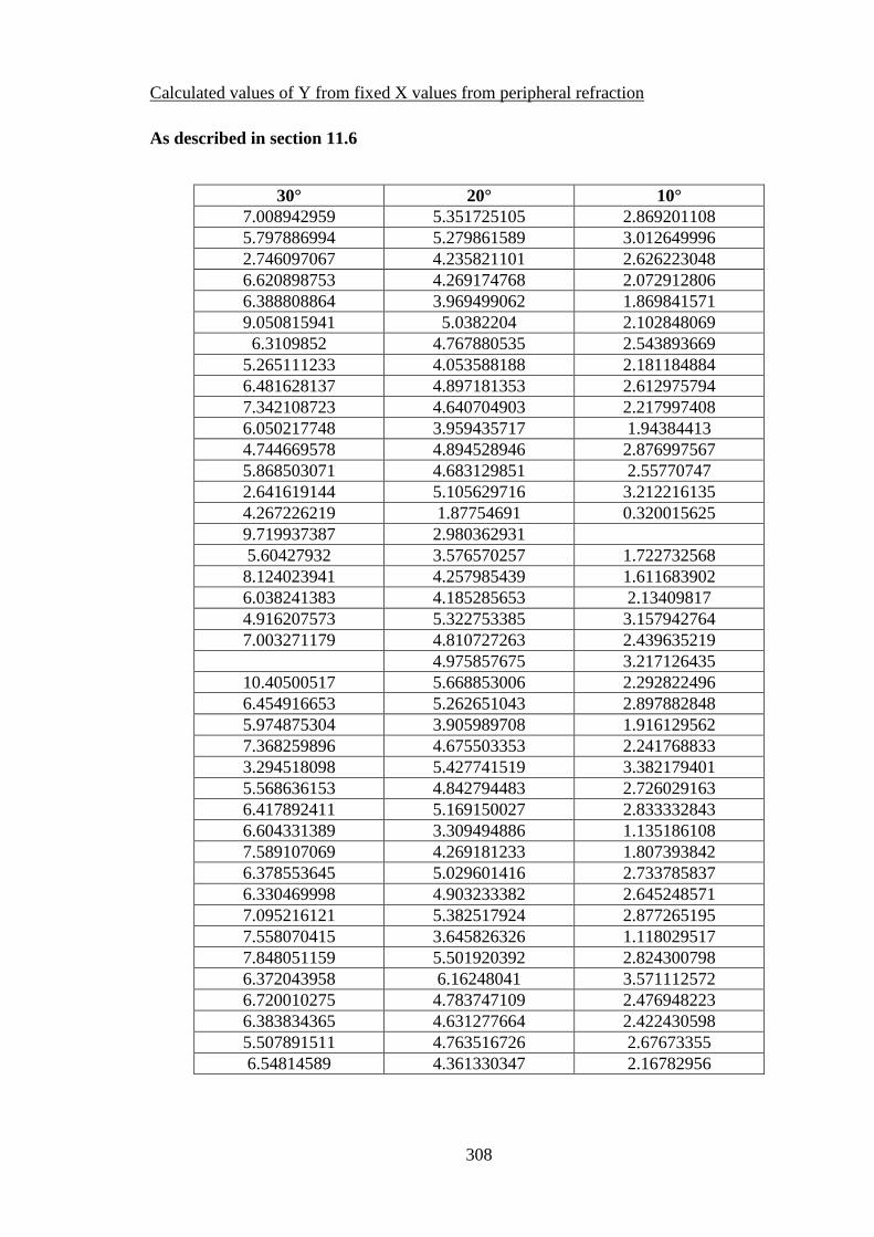
308

Calculated values of Y from fixed X values from peripheral refraction

As described in section 11.6

30° 20° 10°

7.008942959 5.351725105 2.869201108

5.797886994 5.279861589 3.012649996

2.746097067 4.235821101 2.626223048

6.620898753 4.269174768 2.072912806

6.388808864 3.969499062 1.869841571

9.050815941 5.0382204 2.102848069

6.3109852 4.767880535 2.543893669

5.265111233 4.053588188 2.181184884

6.481628137 4.897181353 2.612975794

7.342108723 4.640704903 2.217997408

6.050217748 3.959435717 1.94384413

4.744669578 4.894528946 2.876997567

5.868503071 4.683129851 2.55770747

2.641619144 5.105629716 3.212216135

4.267226219 1.87754691 0.320015625

9.719937387 2.980362931

5.60427932 3.576570257 1.722732568

8.124023941 4.257985439 1.611683902

6.038241383 4.185285653 2.13409817

4.916207573 5.322753385 3.157942764

7.003271179 4.810727263 2.439635219

4.975857675 3.217126435

10.40500517 5.668853006 2.292822496

6.454916653 5.262651043 2.897882848

5.974875304 3.905989708 1.916129562

7.368259896 4.675503353 2.241768833

3.294518098 5.427741519 3.382179401

5.568636153 4.842794483 2.726029163

6.417892411 5.169150027 2.833332843

6.604331389 3.309494886 1.135186108

7.589107069 4.269181233 1.807393842

6.378553645 5.029601416 2.733785837

6.330469998 4.903233382 2.645248571

7.095216121 5.382517924 2.877265195

7.558070415 3.645826326 1.118029517

7.848051159 5.501920392 2.824300798

6.372043958 6.16248041 3.571112572

6.720010275 4.783747109 2.476948223

6.383834365 4.631277664 2.422430598

5.507891511 4.763516726 2.67673355

6.54814589 4.361330347 2.16782956

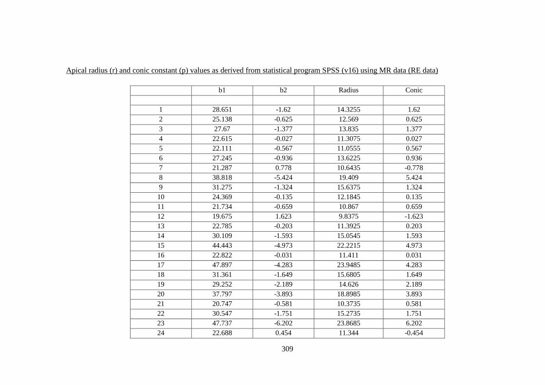
309

Apical radius (r) and conic constant (p) values as derived from statistical program SPSS (v16) using MR data (RE data)

b1 b2 Radius Conic

1 28.651 -1.62 14.3255 1.62

2 25.138 -0.625 12.569 0.625

3 27.67 -1.377 13.835 1.377

4 22.615 -0.027 11.3075 0.027

5 22.111 -0.567 11.0555 0.567

6 27.245 -0.936 13.6225 0.936

7 21.287 0.778 10.6435 -0.778

8 38.818 -5.424 19.409 5.424

9 31.275 -1.324 15.6375 1.324

10 24.369 -0.135 12.1845 0.135

11 21.734 -0.659 10.867 0.659

12 19.675 1.623 9.8375 -1.623

13 22.785 -0.203 11.3925 0.203

14 30.109 -1.593 15.0545 1.593

15 44.443 -4.973 22.2215 4.973

16 22.822 -0.031 11.411 0.031

17 47.897 -4.283 23.9485 4.283

18 31.361 -1.649 15.6805 1.649

19 29.252 -2.189 14.626 2.189

20 37.797 -3.893 18.8985 3.893

21 20.747 -0.581 10.3735 0.581

22 30.547 -1.751 15.2735 1.751

23 47.737 -6.202 23.8685 6.202

24 22.688 0.454 11.344 -0.454

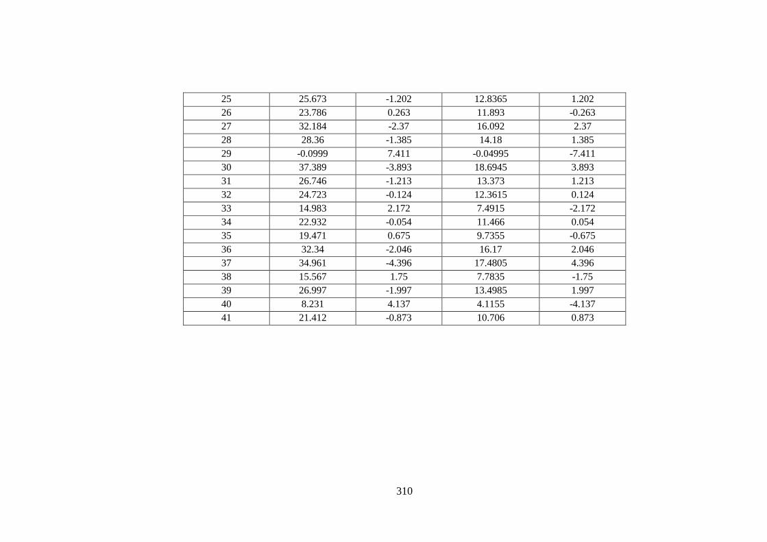
310

25 25.673 -1.202 12.8365 1.202

26 23.786 0.263 11.893 -0.263

27 32.184 -2.37 16.092 2.37

28 28.36 -1.385 14.18 1.385

29 -0.0999 7.411 -0.04995 -7.411

30 37.389 -3.893 18.6945 3.893

31 26.746 -1.213 13.373 1.213

32 24.723 -0.124 12.3615 0.124

33 14.983 2.172 7.4915 -2.172

34 22.932 -0.054 11.466 0.054

35 19.471 0.675 9.7355 -0.675

36 32.34 -2.046 16.17 2.046

37 34.961 -4.396 17.4805 4.396

38 15.567 1.75 7.7835 -1.75

39 26.997 -1.997 13.4985 1.997

40 8.231 4.137 4.1155 -4.137

41 21.412 -0.873 10.706 0.873

311

Calculated values of Y from fixed X values from MRI data

30 degrees eccentricity from the

fovea


fovea


fovea 8.437033128 6.037652855 3.135187395

8.341166435 5.787934865 2.953258793

8.391828305 5.963408522 3.084771872

8.208377873 5.581870762 2.812817538

7.812992596 5.42525439 2.769366805

8.549538958 5.984612068 3.069379416

8.402590541 5.554969235 2.746953767

8.220384273 6.57566532 3.594698875

9.037453048 6.37479995 3.283909256

8.46501013 5.776861259 2.917638172

7.687205871 5.360776101 2.743387049

8.563762742 5.499303701 2.66177901

8.143237053 5.572854457 2.819553599

8.705419617 6.206183272 3.216054648

9.403480882 7.201441439 3.865987261

8.243824167 5.606721288 2.825580029

10.24312363 7.611919259 4.029799313

8.889722442 6.335441926 3.282430121

8.239757345 6.016562839 3.157538202

8.843597724 6.689247402 3.57100231

7.539186422 5.246370517 2.68146928

8.699506589 6.230590309 3.236812089

312

9.342758147 7.35295663 3.993520377

8.479146502 5.672216286 2.827793309

8.12503968 5.756704891 2.972928691

8.571545152 5.772827487 2.890902541

8.662685669 6.316683624 3.312714144

8.509662831 6.041457275 3.123513647

8.158050141 3.775098727 0.970985324

8.774354717 6.64702872 3.550951633

8.314216662 5.882129104 3.035211278

8.533064959 5.820789843 2.939023647

8.013555216 4.981254541 2.34736448

8.251297752 5.61634422 2.83188718

8.015788015 5.306170936 2.626316337

8.854668565 6.382225129 3.326915238

8.07667694 6.314620939 3.42021052

7.886095675 4.981481707 2.379669095

7.928912302 5.783837238 3.033861813

7.848304511 4.386032695 1.840552227

7.497811194 5.280721428 2.717950975

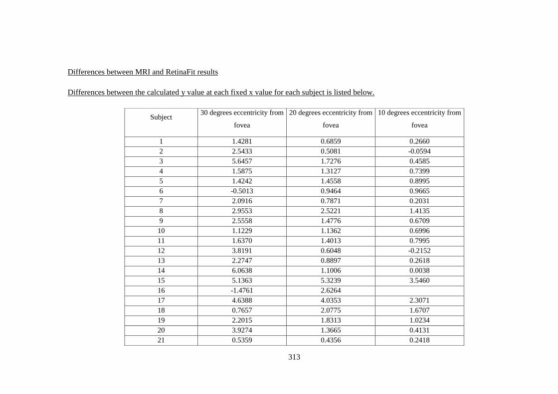
313

Differences between MRI and RetinaFit results

Differences between the calculated y value at each fixed x value for each subject is listed below.

Subject 30 degrees eccentricity from

fovea

20 degrees eccentricity from

fovea

10 degrees eccentricity from

fovea

1 1.4281 0.6859 0.2660

2 2.5433 0.5081 -0.0594

3 5.6457 1.7276 0.4585

4 1.5875 1.3127 0.7399

5 1.4242 1.4558 0.8995

6 -0.5013 0.9464 0.9665

7 2.0916 0.7871 0.2031

8 2.9553 2.5221 1.4135

9 2.5558 1.4776 0.6709

10 1.1229 1.1362 0.6996

11 1.6370 1.4013 0.7995

12 3.8191 0.6048 -0.2152

13 2.2747 0.8897 0.2618

14 6.0638 1.1006 0.0038

15 5.1363 5.3239 3.5460

16 -1.4761 2.6264

17 4.6388 4.0353 2.3071

18 0.7657 2.0775 1.6707

19 2.2015 1.8313 1.0234

20 3.9274 1.3665 0.4131

21 0.5359 0.4356 0.2418

314

22

1.2547 0.0197

23 -1.0622 1.6841 1.7007

24 2.0242 0.4096 -0.0701

25 2.1502 1.8507 1.0568

26 1.2033 1.0973 0.6491

27 5.3682 0.8889 -0.0695

28 2.9410 1.1987 0.3975

29 1.7402 -1.3941 -1.8623

30 2.1700 3.3375 2.4158

31 0.7251 1.6129 1.2278

32 2.1545 0.7912 0.2052

33 1.6831 0.0780 -0.2979

34 1.1561 0.2338 -0.0454

35 0.4577 1.6603 1.5083

36 1.0066 0.8803 0.5026

37 1.7046 0.1521 -0.1509

38 1.1661 0.1977 -0.0973

39 1.5451 1.1526 0.6114

40 2.3404 -0.3775 -0.8362

41 0.9497 0.9194 0.5501

42 2.0450 1.2654 0.5931

43 1.6743 1.1463 0.9293

315

Case Study RC

Case study RC was a 45 year old highly anisomyopic male subject. MSEs were R: -19.76D

L:-2.75D, and thus helped demonstrate an extreme case of myopia in the right eye while

allowing the left eye to act as a control. Ocular biometric data for subject RC are listed in

the table below.

Eye Axial length Corneal curvature A/C depth

Right 27.87 7.32@101/7.29@11 3.50

Left 21.93 7.38@7/ 7.12@97 3.28

Table 36 Biometry data for subject RC measured using the Zeiss IOL Master (in mm)

Results

Figure 131 Peripheral refraction MSE results for subject RC

Consistent with the main study the nasal aspect was shown to be more myopic than the

temporal.

Case Study JP

Case Study JP was a 49 year old highly myopic subject. MSEs were R:-15.50d L:-14.37D.

Ocular biometric data for subject JP is listed in the table below

-25

-20

-15

-10

-5

0

5

-35 -30 -25 -20 -15 -10 -5 0 5 10 15 20 25 30

MS

E i

n D


RIGHT EYE

LEFT EYE

316

Eye Axial length Corneal curvature A/C depth

Right 28.13 7.48@175/7.35@85 3.86

Left 28.78 7.61@163/ 7.28@86 3.72

Table 37 Ocular biometry data for subject JP (in mm)

In addition to taking peripheral refraction measurements as taken in all subjects, peripheral

refractive measures were also taken with soft contact lenses in situ.

Figure 132 MSE results for subject JP, with and without contact lenses in situ

Both eyes showed similar nasal-temporal asymmetries. The nasal region appeared to be

more myopic, which is consistent with results from the main peripheral refraction study. A

similar asymmetry between the nasal and temporal regions was retained with the contact

lenses in situ. As shown on the graph measurements, particularly with the contact lenses in,

were difficult to obtain thus they do not extend to 30˚. Of particular note is the relative

peripheral hyperopic defocus with the contact lens in situ. This subject suffered from

pathological myopia in the form of a longstanding posterior staphyloma.

-20

-15

-10

-5

0

5

10

-35 -30 -25 -20 -15 -10 -5 0 5 10 15 20 25 30

MS

E (

in D

)


LEFT LENS

LEFT EYE

RIGHT EYE

RIGHT LENS

TEMPORALNASAL

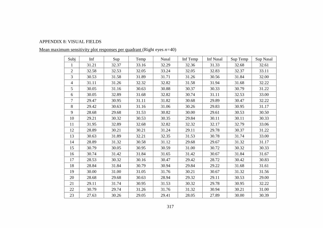
317

APPENDIX 8: VISUAL FIELDS

Mean maximum sensitivity plot responses per quadrant (Right eyes n=40)

Subj Inf Sup Temp Nasal Inf Temp Inf Nasal Sup Temp Sup Nasal

1 31.21 32.37 33.16 32.29 32.36 31.33 32.68 32.61

2 32.58 32.53 32.05 33.24 32.05 32.83 32.37 33.11

3 30.53 31.58 31.89 31.71 31.26 30.56 31.84 32.00

4 31.11 31.26 32.32 32.82 31.58 31.94 31.68 32.22

5 30.05 31.16 30.63 30.88 30.37 30.33 30.79 31.22

6 30.05 32.89 31.68 32.82 30.74 31.11 32.53 33.00

7 29.47 30.95 31.11 31.82 30.68 29.89 30.47 32.22

8 29.42 30.63 31.16 31.06 30.26 29.83 30.95 31.17

9 28.68 29.68 31.53 30.82 30.00 29.61 30.53 30.50

10 29.21 30.32 30.53 30.35 29.84 30.11 30.11 30.33

11 31.95 32.89 32.68 32.82 32.32 32.17 32.79 33.06

12 28.89 30.21 30.21 31.24 29.11 29.78 30.37 31.22

13 30.63 31.89 32.21 32.35 31.53 30.78 31.74 33.00

14 28.89 31.32 30.58 31.12 29.68 29.67 31.32 31.17

15 30.79 30.05 30.95 30.59 31.00 30.72 30.32 30.33

16 30.74 31.42 31.84 31.65 31.42 30.67 31.84 31.67

17 28.53 30.32 30.16 30.47 29.42 28.72 30.42 30.83

18 28.84 31.84 30.79 30.94 29.84 29.22 31.68 31.61

19 30.00 31.00 31.05 31.76 30.21 30.67 31.32 31.56

20 28.68 29.68 30.63 28.94 29.32 29.11 30.53 29.00

21 29.11 31.74 30.95 31.53 30.32 29.78 30.95 32.22

22 30.79 29.74 31.26 31.76 31.32 30.94 30.21 31.00

23 27.63 30.26 29.05 29.41 28.05 27.89 30.00 30.39

318

24 30.53 31.26 30.79 31.12 30.63 30.61 31.26 31.17

25 28.53 31.05 30.32 31.35 29.21 29.28 31.05 31.61

26 29.95 31.26 31.42 31.29 30.95 30.00 31.37 31.56

27 29.00 31.16 30.84 31.65 29.89 30.06 30.95 31.67

28 28.37 31.21 30.47 31.82 28.89 30.00 30.95 31.94

29 29.47 31.32 31.21 31.41 31.11 29.61 31.00 31.61

30 31.00 32.42 31.84 32.12 31.32 31.28 32.16 32.61

31 28.95 30.95 32.00 31.65 31.00 29.61 31.32 31.50

32 28.37 31.42 29.53 30.71 28.58 29.00 30.89 31.50

33 30.05 31.53 31.16 32.71 30.05 31.33 31.79 32.17

34 29.42 32.00 31.26 32.18 30.84 29.72 31.84 32.33

35 30.63 32.68 32.68 31.29 31.26 30.89 33.05 32.11

36 29.32 30.89 31.05 31.71 30.47 29.94 30.68 31.78

37 29.89 31.58 30.16 30.82 30.37 29.61 30.68 31.78

38 31.21 32.16 32.16 32.29 31.95 31.17 32.11 32.56

39 30.58 31.47 31.42 30.82 31.11 30.67 31.58 30.94

40 29.74 30.63 30.42 30.88 29.42 30.83 31.00 30.39

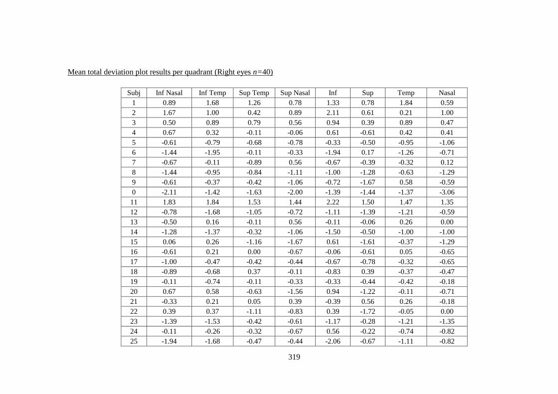
319

Mean total deviation plot results per quadrant (Right eyes n=40)

Subj Inf Nasal Inf Temp Sup Temp Sup Nasal Inf Sup Temp Nasal

1 0.89 1.68 1.26 0.78 1.33 0.78 1.84 0.59

2 1.67 1.00 0.42 0.89 2.11 0.61 0.21 1.00

3 0.50 0.89 0.79 0.56 0.94 0.39 0.89 0.47

4 0.67 0.32 -0.11 -0.06 0.61 -0.61 0.42 0.41

5 -0.61 -0.79 -0.68 -0.78 -0.33 -0.50 -0.95 -1.06

6 -1.44 -1.95 -0.11 -0.33 -1.94 0.17 -1.26 -0.71

7 -0.67 -0.11 -0.89 0.56 -0.67 -0.39 -0.32 0.12

8 -1.44 -0.95 -0.84 -1.11 -1.00 -1.28 -0.63 -1.29

9 -0.61 -0.37 -0.42 -1.06 -0.72 -1.67 0.58 -0.59

0 -2.11 -1.42 -1.63 -2.00 -1.39 -1.44 -1.37 -3.06

11 1.83 1.84 1.53 1.44 2.22 1.50 1.47 1.35

12 -0.78 -1.68 -1.05 -0.72 -1.11 -1.39 -1.21 -0.59

13 -0.50 0.16 -0.11 0.56 -0.11 -0.06 0.26 0.00

14 -1.28 -1.37 -0.32 -1.06 -1.50 -0.50 -1.00 -1.00

15 0.06 0.26 -1.16 -1.67 0.61 -1.61 -0.37 -1.29

16 -0.61 0.21 0.00 -0.67 -0.06 -0.61 0.05 -0.65

17 -1.00 -0.47 -0.42 -0.44 -0.67 -0.78 -0.32 -0.65

18 -0.89 -0.68 0.37 -0.11 -0.83 0.39 -0.37 -0.47

19 -0.11 -0.74 -0.11 -0.33 -0.33 -0.44 -0.42 -0.18

20 0.67 0.58 -0.63 -1.56 0.94 -1.22 -0.11 -0.71

21 -0.33 0.21 0.05 0.39 -0.39 0.56 0.26 -0.18

22 0.39 0.37 -1.11 -0.83 0.39 -1.72 -0.05 0.00

23 -1.39 -1.53 -0.42 -0.61 -1.17 -0.28 -1.21 -1.35

24 -0.11 -0.26 -0.32 -0.67 0.56 -0.22 -0.74 -0.82

25 -1.94 -1.68 -0.47 -0.44 -2.06 -0.67 -1.11 -0.82

320

26 -0.89 -0.32 -0.42 -0.67 -0.33 -0.72 -0.37 -0.82

27 -1.22 -0.74 0.05 -1.06 -1.22 -0.94 -0.11 -0.76

28 -0.06 -1.63 -0.11 0.33 -1.28 0.00 -0.74 0.47

29 -1.39 -0.16 -0.47 -0.50 -1.17 -0.33 -0.37 -0.71

30 0.78 0.58 1.00 1.00 1.11 1.11 0.58 0.65

31 -0.83 0.26 0.05 -0.33 -0.89 -0.56 0.74 -0.12

32 -1.78 -2.37 -0.74 -0.44 -1.72 -0.44 -2.00 -1.00

33 1.00 -0.26 0.47 0.61 0.56 0.22 0.16 1.18

34 -0.94 -0.11 0.37 0.33 -0.78 0.44 -0.21 0.29

35 1.22 1.47 2.47 0.89 1.50 1.89 2.16 0.29

36 0.67 0.26 0.63 0.44 0.11 1.00 0.26 0.53

37 -0.61 0.16 -0.21 0.44 0.22 0.61 -0.53 -0.59

38 -0.83 -1.37 -0.63 -0.06 -0.72 -0.39 -1.26 -0.47

39 0.78 0.84 0.79 -0.39 1.28 0.39 0.68 -0.35

40 -0.39 -1.21 -0.37 -1.11 -0.72 -0.83 -1.05 -0.65

321

Surface area (in mm²)

For Visual fields data (Right eyes)

Subj Nasal Temp Sup Inf Sup Temp Inf Nas Sup Nas Inf Temp

1 189.3 229.4 203.5 227.4 205.0 233.9 226.4 220.5

2 201.5 220.4 249.2 268.3 236.6 225.4 234.9 222.2

3 323.6 320.7 280.1 320.2 275.9 346.5 274.0 337.9

4 225.8 245.9 242.9 225.2 251.3 237.1 224.5 223.6

5 225.2 204.6 229.8 252.7 221.0 254.7 223.9 217.9

6 219.9 235.4 236.0 237.2 241.3 229.1 221.7 226.6

7 245.9 261.7 275.6 257.3 273.1 257.4 252.8 251.0

8 219.7 213.8 231.8 212.6 242.3 270.2 248.6 174.0

9 205.5 208.7 200.0 190.6 200.2 198.4 206.7 197.9

10 216.7 216.1 217.0 205.2 222.1 220.0 221.0 206.0

11 200.6 227.0 208.2 218.2 226.5 213.3 194.4 220.2

12 226.4 251.1 266.0 259.9 260.6 236.5 273.1 261.6

13 211.2 198.6 228.2 202.2 216.3 207.8 222.2 199.3

14 243.2 185.1 199.8 188.6 227.8 236.4 247.8 231.9

15 258.0 268.2 245.9 249.9 275.4 302.9 251.5 284.3

16 213.2 235.4 232.1 217.1 240.6 228.5 201.3 219.0

17 263.8 235.2 229.3 252.5 226.5 274.7 248.1 238.2

18 205.0 203.3 225.0 240.9 216.0 222.6 227.8 222.7

19 218.5 218.7 233.2 229.3 212.3 192.2 222.8 189.1

20 166.1 168.8 163.7 199.3 165.1 199.2 164.8 188.6

21 195.3 192.6 183.6 173.0 193.8 194.0 185.1 172.2

22 225.8 245.9 241.0 228.3 219.5 286.6 220.5 251.6

23 298.7 238.4 262.9 242.4 243.4 284.4 281.7 241.6

24 200.7 221.9 245.8 225.9 245.2 215.0 213.0 221.7

322

25 183.2 194.0 207.1 214.7 198.3 183.1 197.7 187.5

26 188.3 249.9 208.7 238.9 230.3 233.1 221.5 248.8

27 238.7 244.4 228.0 284.3 236.4 281.4 223.3 261.0

28 205.9 194.4 198.6 211.0 196.5 215.6 203.0 196.8

29 202.0 184.4 241.2 194.8 215.2 206.2 208.6 192.9

30 174.5 184.8 160.1 194.9 163.2 190.1 152.8 194.5

31 226.8 257.5 240.8 227.1 233.9 226.8 215.0 215.3

32 243.4 279.2 270.5 272.2 293.7 267.5 250.7 286.4

33 169.2 178.8 179.0 203.8 177.1 186.1 173.3 186.1

34 206.1 223.2 229.1 220.5 240.7 211.7 228.0 188.0

35 149.0 177.8 206.8 164.8 194.6 161.5 175.0 175.9

36 213.2 210.8 256.8 266.3 228.0 251.6 225.4 236.6

37 172.4 214.2 256.6 208.3 234.2 180.1 219.0 219.4

38 183.8 200.0 224.8 210.9 211.6 203.2 208.6 197.0

39 177.8 181.8 229.1 209.4 211.7 181.8 209.5 209.2

40 192.0 228.2 248.3 236.1 267.5 217.0 201.0 219.5

323

Interval Variance for visual fields subjects (Right eyes) derived by multiplying the standard deviation of the data in the posterior 25% of each

quadrant by 1.96

Subj Nasal Temp Sup Inf Sup Temp Inf Nasal Sup Nasal Inf Temp

1 5.18 4.91 5.18 4.91 5.25 4.88 5.17 5.13

2 5.08 5.94 5.94 5.45 6.08 5.15 5.40 5.70

3 6.20 6.85 6.48 5.90 6.49 5.80 6.25 6.18

4 5.11 5.77 6.00 5.40 5.09 5.23 5.38 5.57

5 5.04 5.74 5.83 5.42 5.85 5.21 5.34 5.65

6 5.07 5.65 5.60 5.11 5.74 5.07 5.32 5.42

7 5.36 6.06 5.69 5.38 5.97 5.30 5.49 5.65

8 5.09 5.61 5.79 5.34 5.97 5.22 5.25 5.42

9 5.20 5.82 5.55 4.99 5.77 4.93 5.37 5.44

10 5.02 5.92 5.86 5.43 6.13 5.10 5.31 5.62

11 4.90 5.40 5.37 5.10 5.48 4.97 5.04 5.27

12 5.33 6.04 6.26 5.65 6.13 5.39 6.24 5.97

13 4.88 5.64 5.65 5.23 5.93 5.10 5.22 5.30

14 4.83 5.30 5.62 5.29 5.64 5.34 5.29 5.64

15 5.55 5.82 5.54 5.42 5.92 5.49 5.44 5.57

16 5.06 5.63 5.74 5.26 5.96 5.28 5.13 5.23

17 5.22 6.12 5.55 5.04 5.97 5.02 5.33 5.49

18 4.97 5.44 5.49 5.21 5.66 5.00 5.09 5.40

19 5.19 5.43 5.29 5.36 5.46 4.97 5.04 5.18

20 4.49 5.08 5.30 4.96 5.43 4.58 4.94 4.95

21 4.83 5.13 4.85 4.67 5.19 4.79 4.79 4.75

22 5.05 5.77 5.91 5.40 5.75 4.87 2.77 5.33

23 5.76 5.87 5.74 5.55 5.86 5.54 5.95 5.68

24 5.20 5.79 6.03 5.50 6.22 5.07 5.35 5.30

25 4.69 5.40 5.51 4.80 5.74 4.60 5.06 4.94

324

26 5.13 6.00 5.77 5.06 5.88 5.10 5.46 5.58

27 5.09 5.74 5.98 5.32 6.13 5.26 5.46 5.51

28 5.12 5.48 5.18 4.85 5.63 4.93 5.06 5.03

29 4.76 5.68 5.83 4.75 6.13 4.71 5.41 5.10

30 4.73 5.41 4.69 4.70 5.29 4.87 4.64 5.13

31 5.43 6.12 5.75 5.23 6.14 5.24 5.45 5.54

32 5.40 5.68 5.57 5.29 6.04 5.30 5.34 5.43

33 4.62 5.05 4.95 4.57 5.10 4.41 4.64 5.13

34 5.63 4.93 5.51 5.08 5.51 4.62 5.12 5.01

35 4.44 4.82 4.76 4.77 5.07 4.51 4.50 4.68

36 5.09 5.83 5.36 5.47 6.04 5.22 5.32 5.56

37 4.70 5.71 5.48 5.15 5.86 4.79 4.99 5.42

38 4.65 5.46 5.76 5.16 5.79 4.71 5.10 5.37

39 5.00 5.24 5.84 5.24 5.25 5.01 5.38 5.38

40 4.87 5.19 5.79 4.66 5.69 5.13 5.19 5.41

325

Visual fields sensitivity per quadrant for left eyes n=42 (Sita Standard 30-2)

1 Inf Sup Temp Nasal Inf Temp Inf Nas Sup Temp Sup Nas

2 30.79 30.58 31.79 31.53 31.37 31.06 31.21 31.00

3 30.53 31.63 31.84 32.59 31.53 30.94 31.47 32.56

4 31.05 31.42 30.95 32.00 31.05 31.22 31.05 32.06

5 31.16 31.32 31.58 32.65 31.37 31.39 31.42 32.44

6 28.95 31.32 29.89 31.29 29.26 29.78 30.74 31.61

7 29.42 31.79 31.84 31.94 30.58 30.50 32.26 31.56

8 28.42 29.84 29.84 31.06 29.42 29.00 29.63 31.00

9 27.89 30.68 29.68 30.71 28.47 28.61 30.53 31.28

10 27.84 29.79 29.68 30.06 28.37 28.78 30.26 29.89

11 29.37 30.42 30.63 31.53 29.68 30.50 31.05 30.61

12 30.84 32.37 31.26 33.47 31.11 31.44 32.47 32.78

13 27.95 31.11 30.63 30.94 29.95 28.44 30.47 31.67

14 30.63 31.89 31.53 32.00 30.95 31.33 31.47 32.28

15 30.05 32.74 31.26 32.53 30.74 31.50 31.47 32.83

16 28.58 30.68 30.05 31.00 29.16 29.89 29.95 31.28

17 28.74 31.37 30.47 31.71 29.84 29.56 30.68 32.11

18 29.42 31.16 30.74 31.24 29.63 30.78 31.16 30.94

19 27.84 29.89 29.21 29.94 28.84 28.17 29.37 30.44

20 30.05 30.53 30.21 32.12 29.95 30.78 30.37 31.72

21 28.89 29.32 30.00 29.35 29.58 29.11 29.47 29.39

22 30.26 30.63 31.37 31.82 30.89 30.67 30.95 31.50

23 30.00 30.79 29.47 32.06 29.68 30.72 29.89 31.94

24 27.84 31.32 29.00 32.12 28.53 29.11 30.53 31.94

25 29.58 30.74 30.21 30.76 29.95 30.00 30.37 30.94

326

26 27.42 31.74 30.21 30.59 29.26 27.94 31.00 31.67

27 29.53 30.84 29.84 31.65 29.89 30.00 30.05 31.83

28 29.00 30.42 30.79 31.29 29.68 29.78 30.37 31.61

29 28.47 31.37 31.63 30.88 29.68 29.44 31.47 31.72

30 27.53 30.68 31.26 31.29 29.68 29.00 30.74 31.22

31 30.47 32.05 31.26 31.65 31.16 30.33 31.42 32.50

32 29.16 31.11 30.74 31.82 30.53 29.22 30.89 32.06

33 28.79 30.95 29.53 31.94 29.26 29.89 30.47 31.44

327

Visual fields sensitivity Sita Standard 10-2 (in dB)

Subj 1 1 2 2 3 3 4 4 5 5 6 6 7 7 8 8 9 9

Location R L R L R L R L R L R L R L R L R L

1 34 36 32 32 33 32 31 31 33 31 31 33 33 33 32 31 29 30

2 33 33 31 33 32 34 32 32 31 31 34 31 32 32 32 31 31 27

3 33 38 34 33 34 31 31 31 30 31 34 33 31 32 32 32 32 32

4 33 32 33 33 33 34 33 31 33 33 31 31 32 33 31 33 30 31

5 33 32 32 33 32 32 31 33 33 34 32 32 34 34 33 31 33 31

6 33 34 32 32 32 34 31 32 30 33 32 34 32 33 32 31 32 31

7 34 33 33 32 34 31 31 34 31 33 33 33 33 33 31 33 32 33

8 33 33 32 32 33 33 28 32 32 32 33 32 31 31 31 32 33 31

9 32 34 34 33 34 33 32 31 34 34 32 32 32 32 33 34 34 32

10 34 35 33 33 33 34 32 32 31 34 33 32 33 31 33 33 33 34

11 35 33 34 35 34 34 31 33 32 34 34 34 33 32 34 32 34 33

12 34 34 35 35 33 34 33 32 32 33 35 35 34 33 33 32 35 34

13 33 33 33 33 33 34 34 31 32 32 33 34 33 31 33 32 35 33

14 34 33 33 34 33 33 33 33 31 32 34 33 33 31 33 33 33 33

15 34 32 33 33 34 34 30 32 31 33 34 34 34 31 32 32 32 32

16 34 36 33 33 34 33 33 33 33 32 32 35 34 33 33 32 29 31

17 34 34 35 35 33 34 33 32 33 32 34 32 35 37 34 32 33 34

18 35 34 34 33 34 36 33 33 32 33 34 34 33 33 35 33 34 35

19 35 34 35 33 36 35 33 34 34 33 34 35 33 33 35 34 35 35

20 35 33 34 34 34 36 33 33 34 33 34 34 34 32 34 34 34 35

328

21 34 33 34 33 35 35 33 32 34 34 34 36 32 32 35 34 34 34

22 33 34 34 34 34 33 33 33 33 33 35 35 33 35 35 34 35 35

23 35 34 35 35 32 34 34 33 33 33 33 34 34 34 33 34 34 34

24 34 34 34 33 33 33 31 32 34 34 31 32 36 31 32 34 33 32

25 33 35 33 33 33 31 34 33 33 32 34 33 32 33 34 31 32 35

26 35 33 33 33 34 32 33 32 34 33 33 33 34 33 35 33 33 33

27 34 35 35 35 33 34 34 33 33 33 34 35 35 34 32 33 35 35

28 35 34 34 35 33 35 35 35 34 34 36 33 35 34 36 34 34 34

29 34 35 35 35 35 35 34 33 34 33 36 33 36 35 36 34 35 34

30 35 35 35 34 33 35 33 34 36 36 35 35 34 35 36 36 36 35

31 34 34 34 31 36 35 35 34 35 35 35 36 37 34 34 36 36 34

32 34 33 34 33 34 35 34 34 37 34 34 36 34 35 33 35 36 33

33 35 34 33 32 34 35 32 34 33 34 34 32 33 33 32 33 33 34

34 34 32 35 32 33 34 33 34 31 32 34 33 33 33 33 32 32 31

35 33 34 35 35 32 33 31 32 32 33 34 32 32 32 34 33 33 32

36 34 33 33 34 33 33 32 34 33 34 35 34 35 33 35 33 33 33

37 34 35 34 35 33 34 34 33 35 33 34 34 35 33 34 35 35 34

38 33 34 36 34 32 35 35 34 34 34 36 32 35 35 36 34 38 36

39 34 35 36 36 34 36 34 33 35 35 34 32 35 37 36 33 353 36

40 34 36 36 35 33 35 35 33 34 36 34 36 36 36 36 36 6 36

41 36 35 35 34 36 36 36 33 35 34 36 35 34 35 33 36 36 35

42 36 34 34 35 34 36 36 33 35 33 34 35 33 34 33 34 34 34

43 34 34 34 33 34 33 33 34 34 32 34 34 33 34 32 32 34 32

44 34 32 33 33 33 33 34 34 32 32 34 35 32 32 34 34 31 32

45 35 33 34 35 34 34 32 32 33 33 33 34 33 32 34 32 34 33

329

46 34 34 35 34 33 36 32 34 34 32 34 33 33 32 34 33 35 35

47 35 35 35 35 34 35 32 35 35 33 35 33 33 33 35 33 34 34

48 35 34 35 35 34 34 34 35 34 34 34 34 34 33 34 34 34 34

49 34 34 34 34 35 36 36 33 34 35 34 36 35 34 36 34 34 35

50 36 35 35 35 35 35 35 34 34 35 35 34 35 34 35 35 35 34

51 34 34 34 34 34 34 34 34 33 34 34 33 34 34 34 34 33 33

52 36 37 32 34 33 34 32 34 34 34 34 33 33 37 34 34 32 30

53 37 34 34 33 32 36 34 32 32 31 32 34 34 32 34 31 34 33

54 34 33 34 33 33 34 33 34 33 32 33 33 34 31 33 32 34 33

55 36 34 33 34 33 34 33 34 34 34 34 33 35 33 34 35 33 35

56 36 35 34 33 32 33 34 33 33 33 33 34 35 36 33 35 32 33

57 35 33 33 33 33 33 34 32 34 34 33 34 32 35 33 35 33 34

58 34 34 34 34 34 34 34 33 33 32 34 35 32 34 34 34 34 33

59 33 33 35 33 35 33 33 32 33 34 32 34 34 33 33 33 32 33

60 35 34 35 34 33 34 32 34 34 34 32 33 33 33 34 32 31 33

61 34 32 33 33 34 33 33 33 32 31 32 33 30 33 32 33 34 33

62 33 33 35 34 33 34 30 33 33 33 32 31 31 32 33 33 33 32

63 34 35 33 32 33 34 32 32 34 32 32 33 32 33 32 33 33 32

64 33 34 33 32 32 33 32 31 32 32 34 33 33 32 32 31 34 34

65 33 33 35 33 33 34 32 31 32 34 32 32 33 31 34 33 33 32

66 33 33 34 32 33 32 34 31 32 34 32 32 34 35 36 34 32 32

67 33 32 33 31 33 34 29 31 32 33 31 33 34 33 33 32 33 31

68 34 30 33 31 32 32 31 30 33 32 33 33 33 33 34 34 33 32

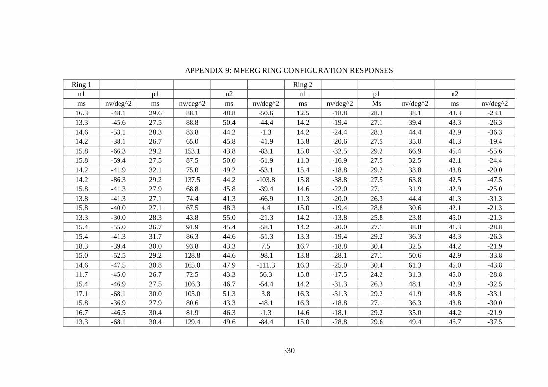
330

APPENDIX 9: MFERG RING CONFIGURATION RESPONSES

Ring 1

Ring 2

n1

p1

n2

n1

p1

n2

ms nv/deg^2 ms nv/deg^2 ms nv/deg^2 ms nv/deg^2 Ms nv/deg^2 ms nv/deg^2

16.3 -48.1 29.6 88.1 48.8 -50.6 12.5 -18.8 28.3 38.1 43.3 -23.1

13.3 -45.6 27.5 88.8 50.4 -44.4 14.2 -19.4 27.1 39.4 43.3 -26.3

14.6 -53.1 28.3 83.8 44.2 -1.3 14.2 -24.4 28.3 44.4 42.9 -36.3

14.2 -38.1 26.7 65.0 45.8 -41.9 15.8 -20.6 27.5 35.0 41.3 -19.4

15.8 -66.3 29.2 153.1 43.8 -83.1 15.0 -32.5 29.2 66.9 45.4 -55.6

15.8 -59.4 27.5 87.5 50.0 -51.9 11.3 -16.9 27.5 32.5 42.1 -24.4

14.2 -41.9 32.1 75.0 49.2 -53.1 15.4 -18.8 29.2 33.8 43.8 -20.0

14.2 -86.3 29.2 137.5 44.2 -103.8 15.8 -38.8 27.5 63.8 42.5 -47.5

15.8 -41.3 27.9 68.8 45.8 -39.4 14.6 -22.0 27.1 31.9 42.9 -25.0

13.8 -41.3 27.1 74.4 41.3 -66.9 11.3 -20.0 26.3 44.4 41.3 -31.3

15.8 -40.0 27.1 67.5 48.3 4.4 15.0 -19.4 28.8 30.6 42.1 -21.3

13.3 -30.0 28.3 43.8 55.0 -21.3 14.2 -13.8 25.8 23.8 45.0 -21.3

15.4 -55.0 26.7 91.9 45.4 -58.1 14.2 -20.0 27.1 38.8 41.3 -28.8

15.4 -41.3 31.7 86.3 44.6 -51.3 13.3 -19.4 29.2 36.3 43.3 -26.3

18.3 -39.4 30.0 93.8 43.3 7.5 16.7 -18.8 30.4 32.5 44.2 -21.9

15.0 -52.5 29.2 128.8 44.6 -98.1 13.8 -28.1 27.1 50.6 42.9 -33.8

14.6 -47.5 30.8 165.0 47.9 -111.3 16.3 -25.0 30.4 61.3 45.0 -43.8

11.7 -45.0 26.7 72.5 43.3 56.3 15.8 -17.5 24.2 31.3 45.0 -28.8

15.4 -46.9 27.5 106.3 46.7 -54.4 14.2 -31.3 26.3 48.1 42.9 -32.5

17.1 -68.1 30.0 105.0 51.3 3.8 16.3 -31.3 29.2 41.9 43.8 -33.1

15.8 -36.9 27.9 80.6 43.3 -48.1 16.3 -18.8 27.1 36.3 43.8 -30.0

16.7 -46.5 30.4 81.9 46.3 -1.3 14.6 -18.1 29.2 35.0 44.2 -21.9

13.3 -68.1 30.4 129.4 49.6 -84.4 15.0 -28.8 29.6 49.4 46.7 -37.5

331

Ring 3

Ring 4

n1

p1

n2

n1

p1

n2


13.8 -11.3 28.8 18.1 42.9 -15.0 15.4 -10.6 28.0 14.4 41.3 -10.0

15.0 -11.9 28.3 21.3 42.5 -16.3 14.6 -8.8 29.6 14.4 42.5 -12.5

13.8 -12.5 28.3 25.6 42.1 -23.1 14.6 -9.4 28.8 15.0 42.1 -15.0

13.8 -13.1 26.3 23.8 40.4 -15.0 13.8 -9.4 29.2 13.1 41.6 -10.0

15.8 -20.6 28.3 33.8 42.9 -36.9 15.0 -16.9 28.8 23.1 43.8 -19.4

14.2 -11.3 27.1 18.8 41.3 -15.6 12.9 -8.1 28.3 10.6 40.8 -10.6

13.3 -9.4 27.9 16.9 40.4 -13.1 13.8 -6.3 27.1 9.4 40.4 -10.0

15.0 -18.8 29.2 32.5 41.7 -28.8 15.0 -12.5 28.3 26.3 42.5 -17.5

14.6 -13.8 29.6 20.0 42.5 -15.6 14.2 -9.4 29.6 15.0 42.1 -11.3

11.7 -8.8 25.8 21.3 39.6 -18.8 12.5 -6.3 26.3 11.3 40.8 -10.0

14.6 -12.5 29.6 20.6 41.7 -13.8 15.4 -11.3 28.8 14.4 42.5 -11.9

14.2 -10.0 27.5 16.3 41.7 -11.3 14.2 -6.3 28.3 10.0 40.8 -10.0

14.2 -14.4 27.1 25.0 40.4 -19.4 14.6 -12.5 28.3 16.9 41.3 -14.4

13.8 -11.3 29.6 17.5 42.5 -15.6 15.8 -9.4 29.6 13.8 41.7 -11.3

15.8 -12.5 29.6 18.8 43.3 -17.5 13.3 -8.8 30.8 12.5 44.2 -10.6

14.2 -15.0 27.9 26.5 42.1 -20.6 14.2 -10.0 27.9 16.9 41.7 -15.0

16.7 -16.3 29.2 28.8 43.3 -23.8 16.3 -11.3 31.3 16.3 43.3 -11.3

15.8 -11.3 25.8 18.8 40.0 -18.8 13.3 -11.3 27.5 15.0 39.2 -8.8

15.0 -16.9 27.5 26.9 40.4 -19.4 13.8 -11.9 25.8 15.0 40.0 -11.3

15.0 -18.1 29.6 25.0 41.3 -18.8 14.2 -12.5 29.2 20.0 41.3 -13.1

12.9 -11.3 27.9 18.8 40.4 -14.4 14.6 -8.8 28.3 14.4 42.1 -11.9

15.4 -10.6 29.6 16.3 42.9 -14.4 14.2 -8.1 27.9 12.5 41.7 -9.4

16.3 -18.1 29.2 26.9 43.8 -22.5 15.8 -12.5 28.3 18.1 42.9 -14.4

332

Ring 5

Ring 6

n1

p1

n2

n1

p1

n2

ms nv/deg^2 ms nv/deg^2 ms nv/deg^2 ms nv/deg^2 ms nv/deg^2 ms nv/deg^2

14.2 -8.8 28.8 12.5 42.1 -10.0 14.2 -7.5 28.3 8.8 41.7 -7.5

15.4 -7.5 30.8 10.0 43.3 -10.6 15.4 -6.3 30.8 7.5 42.5 -6.9

15.0 -7.5 29.6 11.3 42.5 -10.0 15.4 -6.9 30.8 8.1 42.5 -7.5

15.4 -8.8 28.3 9.4 42.5 -8.1 14.6 -6.3 29.2 8.1 42.5 -6.9

15.0 -12.5 27.9 17.5 44.2 -15.0 15.0 -6.9 29.6 10.6 45.0 -9.4

13.3 -6.3 27.9 8.1 42.5 -6.9 14.2 -5.0 29.2 5.6 40.8 -5.6

11.7 -5.0 27.9 8.8 41.7 -6.3 13.8 -4.4 29.2 5.6 42.5 -6.3

15.0 -11.3 29.2 17.5 43.3 -15.0 14.2 -7.5 29.2 11.3 42.5 -8.8

14.6 -7.5 30.0 10.6 42.9 -8.8 15.0 -6.3 30.8 7.5 43.3 -7.5

14.2 -6.3 25.4 10.0 40.0 -6.9 11.7 -3.8 29.2 5.0 42.1 -5.6

15.0 -7.5 30.0 11.3 43.3 -9.4 15.8 -7.5 30.0 11.3 43.3 -10.0

14.2 -6.3 29.2 7.5 43.3 -8.8 14.2 -5.0 29.2 6.3 41.7 -6.3

14.6 -9.4 28.3 13.1 42.1 -11.3 14.6 -7.5 29.2 8.8 42.5 -8.8

15.4 -7.5 30.0 10.0 42.9 -8.1 15.0 -6.3 30.8 6.3 43.3 -6.3

16.3 -8.1 30.8 10.0 43.8 -8.1 16.3 -5.0 32.1 4.4 43.3 -5.0

15.0 -10.0 28.3 12.5 41.7 -10.6 15.0 -8.1 28.8 9.4 41.7 -8.1

17.5 -8.8 32.5 11.9 47.5 -11.3 17.5 -5.6 34.2 8.1 47.9 -8.1

15.0 -8.8 29.2 10.0 40.0 -7.5 12.5 -6.3 29.2 8.8 40.8 6.3

15.4 -10.0 29.2 11.9 42.9 -10.0 15.0 -8.1 25.8 11.3 42.1 -7.5

15.4 -10.0 30.0 13.8 41.7 -10.0 15.0 -5.6 30.0 7.5 41.3 -5.6

15.4 -8.1 28.8 10.6 42.1 -8.8 14.6 -6.3 28.8 8.8 42.5 -7.5

14.6 -6.9 30.4 8.1 42.5 -6.9 14.2 -5.6 30.4 8.1 42.1 -6.3

16.3 -11.3 30.0 12.5 43.8 -10.0 14.2 -7.5 30.0 10.0 42.9 -7.5

333

+Q Configuration responses

INFERIOR NASAL

INFERIOR TEMP

n1

p1

n2

n1

p1

n2


14.6 -8.1 28.8 10.0 42.1 -8.1 16.1 -7.5 28.3 11.3 42.1 -8.8

15.8 -6.9 30.4 8.8 42.9 -8.1 15.8 -8.8 30.4 12.5 42.9 -10.6

14.2 -6.9 29.6 10.6 42.1 -10.0 15.4 -6.9 29.2 12.5 41.7 -10.6

14.2 -6.9 28.3 9.4 42.1 -6.9 15.0 -8.1 28.3 10.6 41.3 -8.1

15.4 -8.8 28.8 13.8 44.2 -11.3 15.8 -10.6 29.2 15.6 44.2 -13.8

13.8 -5.6 28.3 6.3 40.8 -6.9 12.5 -6.3 29.2 8.8 39.6 -6.9

14.2 -5.0 27.9 6.9 41.7 -6.3 13.3 -5.6 28.3 8.1 41.7 -7.5

15.0 -10.0 30.0 15.0 42.5 -11.3 15.8 -11.3 29.2 17.5 42.5 -12.5

15.0 -7.5 30.0 8.8 42.9 -7.5 14.2 -6.9 29.6 11.9 42.5 -8.8

12.9 -3.8 27.9 6.3 39.2 -5.0 15.0 -6.3 26.7 9.4 38.3 -7.5

15.4 -8.1 30.8 10.6 43.8 -9.4 15.8 -8.8 29.2 13.1 42.5 -11.3

13.3 -6.3 29.2 6.3 39.2 -3.8 15.8 -6.3 27.5 8.8 40.8 -7.5

13.3 -7.5 28.8 10.0 42.5 -8.8 15.0 -9.4 28.8 13.1 42.5 -12.5

15.0 -6.9 30.0 7.5 42.1 -6.3 15.8 -7.5 30.0 9.4 42.5 -9.4

13.8 -4.4 31.3 6.3 41.7 -5.0 15.4 -5.0 30.4 7.5 42.5 -5.6

14.6 -8.8 27.9 11.9 42.1 -8.8 15.0 -10.0 27.1 14.4 41.3 -11.3

17.5 -8.1 33.3 11.3 47.9 -8.8 15.8 -6.9 32.1 11.3 45.8 -0.6

13.3 -6.3 27.5 8.8 40.8 -7.5 15.8 -8.8 29.2 11.3 40.8 -8.8

13.8 -8.8 27.1 10.6 41.3 -8.1 15.4 -9.4 27.5 13.8 42.5 -9.4

12.5 -7.5 30.0 10.6 40.8 -6.9 15.4 -8.8 29.6 11.3 41.7 -9.4

14.2 -6.9 29.2 8.8 42.5 -8.1 12.9 -6.9 28.8 11.9 42.1 -9.4

15.0 -5.6 29.2 7.5 42.9 -5.6 14.6 -8.1 29.6 11.9 42.1 -8.8

15.4 -8.8 30.0 10.6 45.0 -8.1 15.4 -9.4 30.0 13.1 42.9 -11.3

334

SUPERIOR NASAL

SUPERIOR TEMP

n1

p1

n2

n1

p1

n2


13.8 -8.8 30.4 10.6 41.3 -8.1 14.6 -10.6 27.9 13.8 41.7 -10.6

14.2 -6.3 30.0 10.0 43.3 -9.4 15.8 -8.8 28.3 12.5 42.9 -11.3

14.2 -7.5 29.6 10.6 42.1 -9.4 15.0 -9.4 30.0 13.1 41.7 -11.3

13.8 -7.5 30.0 10.0 41.7 -7.5 15.0 -8.1 28.3 12.5 42.9 -9.4

15.0 -11.3 28.8 16.3 43.8 -14.4 15.0 -12.5 28.7 19.4 43.3 -15.6

12.1 -5.6 27.1 7.5 40.8 -6.9 15.0 -8.1 28.8 10.0 41.3 -8.8

13.8 -5.6 29.2 6.9 41.7 -6.9 12.5 -5.6 27.1 10.0 40.4 -8.1

12.5 -8.8 29.2 15.0 44.2 -13.8 15.8 -12.5 28.3 20.0 43.3 -15.0

15.0 -7.5 30.4 9.4 42.9 -8.1 14.6 -9.4 30.0 12.5 42.9 -10.6

12.5 -5.0 26.3 7.5 40.4 -6.3 12.1 -6.9 26.7 12.5 40.0 -8.8

15.8 -8.1 30.8 11.9 43.3 -8.8 15.4 -10.0 29.6 13.8 28.3 -12.5

14.2 -6.3 28.3 8.8 41.7 -8.8 15.0 -7.5 29.2 10.0 42.5 -10.0

14.6 -9.4 28.8 11.3 42.5 -11.3 14.2 -10.6 27.9 16.3 41.7 -12.5

15.0 -7.5 30.4 9.4 43.7 -7.5 16.3 -9.4 30.4 11.3 42.5 -9.4

12.5 -6.9 30.4 10.0 42.9 -9.4 15.4 -8.8 30.8 11.3 44.2 -9.4

12.9 -7.5 29.2 11.3 42.5 -11.3 13.8 -10.6 27.5 16.3 41.7 -11.9

17.5 -7.5 33.8 11.3 47.5 -9.4 17.5 -10.0 31.3 15.0 46.3 -13.1

15.8 -7.5 29.2 8.8 40.0 -6.3 15.8 -11.3 28.3 13.8 40.0 -10.0

15.0 -9.4 29.6 10.6 41.3 -8.8 14.2 -10.6 26.3 16.9 40.4 -10.6

15.0 -9.4 29.6 13.8 41.7 -7.5 14.6 -9.4 30.4 13.1 41.3 -10.0

15.4 -7.5 28.8 10.0 42.5 -10.0 14.6 -8.1 28.8 12.5 41.3 -9.4

13.8 -6.3 29.2 8.1 42.1 -6.3 15.0 -8.1 30.4 11.3 43.8 -9.4

15.4 -10.0 30.8 12.5 44.2 -10.0 15.4 -12.5 28.8 16.9 42.9 -11.9

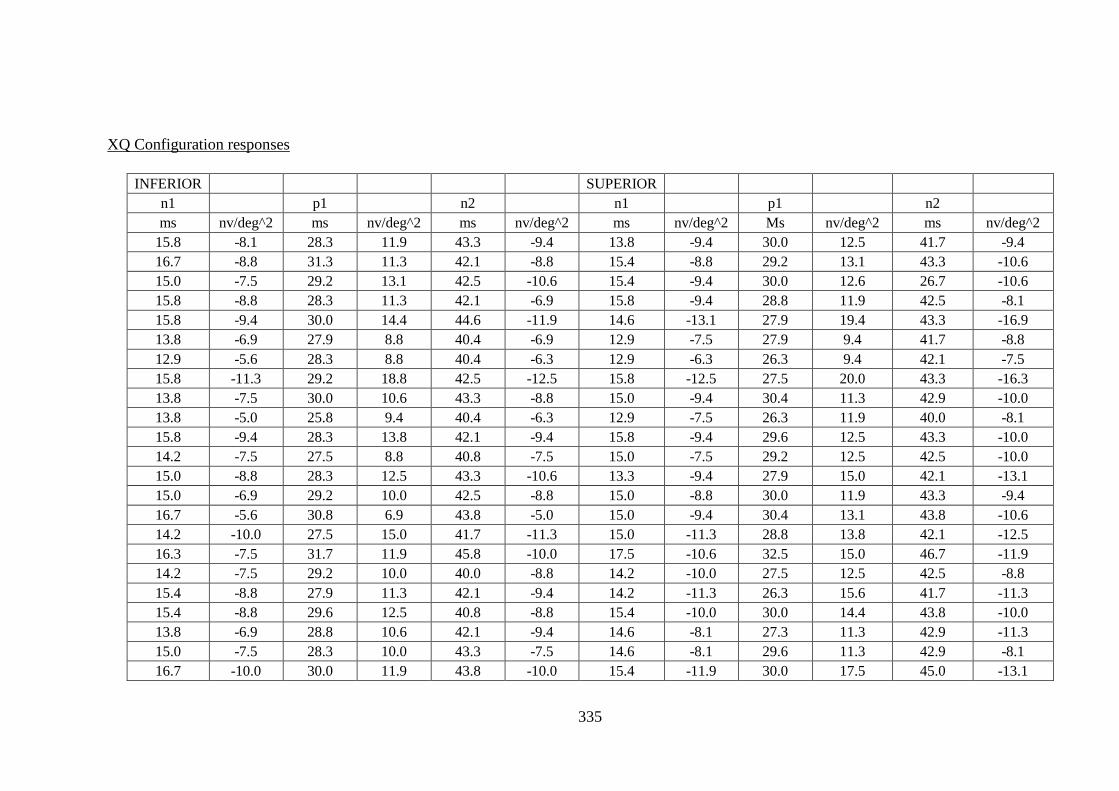
335

XQ Configuration responses

INFERIOR

SUPERIOR

n1

p1

n2

n1

p1

n2


15.8 -8.1 28.3 11.9 43.3 -9.4 13.8 -9.4 30.0 12.5 41.7 -9.4

16.7 -8.8 31.3 11.3 42.1 -8.8 15.4 -8.8 29.2 13.1 43.3 -10.6

15.0 -7.5 29.2 13.1 42.5 -10.6 15.4 -9.4 30.0 12.6 26.7 -10.6

15.8 -8.8 28.3 11.3 42.1 -6.9 15.8 -9.4 28.8 11.9 42.5 -8.1

15.8 -9.4 30.0 14.4 44.6 -11.9 14.6 -13.1 27.9 19.4 43.3 -16.9

13.8 -6.9 27.9 8.8 40.4 -6.9 12.9 -7.5 27.9 9.4 41.7 -8.8

12.9 -5.6 28.3 8.8 40.4 -6.3 12.9 -6.3 26.3 9.4 42.1 -7.5

15.8 -11.3 29.2 18.8 42.5 -12.5 15.8 -12.5 27.5 20.0 43.3 -16.3

13.8 -7.5 30.0 10.6 43.3 -8.8 15.0 -9.4 30.4 11.3 42.9 -10.0

13.8 -5.0 25.8 9.4 40.4 -6.3 12.9 -7.5 26.3 11.9 40.0 -8.1

15.8 -9.4 28.3 13.8 42.1 -9.4 15.8 -9.4 29.6 12.5 43.3 -10.0

14.2 -7.5 27.5 8.8 40.8 -7.5 15.0 -7.5 29.2 12.5 42.5 -10.0

15.0 -8.8 28.3 12.5 43.3 -10.6 13.3 -9.4 27.9 15.0 42.1 -13.1

15.0 -6.9 29.2 10.0 42.5 -8.8 15.0 -8.8 30.0 11.9 43.3 -9.4

16.7 -5.6 30.8 6.9 43.8 -5.0 15.0 -9.4 30.4 13.1 43.8 -10.6

14.2 -10.0 27.5 15.0 41.7 -11.3 15.0 -11.3 28.8 13.8 42.1 -12.5

16.3 -7.5 31.7 11.9 45.8 -10.0 17.5 -10.6 32.5 15.0 46.7 -11.9

14.2 -7.5 29.2 10.0 40.0 -8.8 14.2 -10.0 27.5 12.5 42.5 -8.8

15.4 -8.8 27.9 11.3 42.1 -9.4 14.2 -11.3 26.3 15.6 41.7 -11.3

15.4 -8.8 29.6 12.5 40.8 -8.8 15.4 -10.0 30.0 14.4 43.8 -10.0

13.8 -6.9 28.8 10.6 42.1 -9.4 14.6 -8.1 27.3 11.3 42.9 -11.3

15.0 -7.5 28.3 10.0 43.3 -7.5 14.6 -8.1 29.6 11.3 42.9 -8.1

16.7 -10.0 30.0 11.9 43.8 -10.0 15.4 -11.9 30.0 17.5 45.0 -13.1

336

NASAL

TEMPORAL

n1

p1

n2

n1

p1

n2


13.3 -7.5 28.8 10.0 41.7 -7.5 14.6 -9.4 28.3 11.3 41.7 -10.0

14.6 -5.6 30.4 7.5 43.3 -7.5 15.8 -8.1 30.8 11.3 42.9 -11.3

14.6 -6.9 29.6 8.8 42.5 -8.8 15.4 -8.8 29.6 12.5 42.5 -11.9

15.4 -7.5 30.4 8.1 41.7 -7.5 15.4 -8.1 28.3 11.3 42.5 -8.8

14.6 -9.4 28.3 13.8 43.8 -12.5 14.2 -10.6 27.9 17.5 44.2 -14.4

12.1 -4.4 29.6 5.0 40.8 -6.3 15.4 -7.5 29.2 9.4 41.3 -8.1

15.0 -5.0 28.3 5.6 41.7 -6.9 13.8 -5.6 27.1 9.4 42.5 -8.8

15.0 -8.8 30.0 13.8 42.5 -11.3 15.8 -11.3 28.3 16.3 43.3 -13.8

15.0 -6.3 30.0 7.5 43.3 -7.5 16.3 -8.8 30.0 11.9 42.9 -10.6

12.9 -3.8 29.2 5.0 40.4 -5.0 15.0 -6.9 25.8 10.6 39.2 -8.8

16.3 -6.9 30.8 10.6 43.3 -8.8 15.4 -8.8 30.0 13.8 42.5 -12.5

14.2 -6.3 31.7 3.8 40.0 -5.0 15.0 -6.3 29.2 8.8 42.5 -10.0

15.0 -8.8 29.6 8.1 42.1 -8.1 14.6 -10.0 28.8 14.4 42.1 -12.5

14.6 -6.3 30.0 6.9 42.9 -5.6 15.0 -7.5 30.0 10.6 42.5 -9.4

12.9 0.0 30.0 7.5 42.9 -6.9 14.6 -6.3 30.8 7.5 42.5 -6.9

15.0 -6.9 28.8 9.4 42.1 -9.4 14.2 -9.4 27.5 15.0 41.7 -11.9

18.3 -6.9 34.2 9.4 47.1 -6.9 17.5 -8.1 32.9 11.3 46.3 -11.3

13.3 -6.3 29.2 7.5 42.5 -6.3 15.0 -10.0 27.5 13.8 40.0 -8.8

14.2 -7.5 30.4 9.4 41.7 -8.1 13.8 -10.0 26.7 16.9 42.1 -10.6

15.8 -7.5 29.6 13.1 41.3 -8.8 15.8 -9.4 30.0 11.3 41.3 -9.4

14.2 -6.9 28.3 9.4 42.9 -7.5 15.4 -8.1 28.8 11.9 41.7 -9.4

15.0 -5.6 29.6 6.9 42.9 -5.6 14.6 -8.1 29.6 11.9 42.5 -9.4

15.4 -8.1 30.4 10.6 42.5 -7.5 15.4 -11.3 27.5 15.6 42.9 -11.9

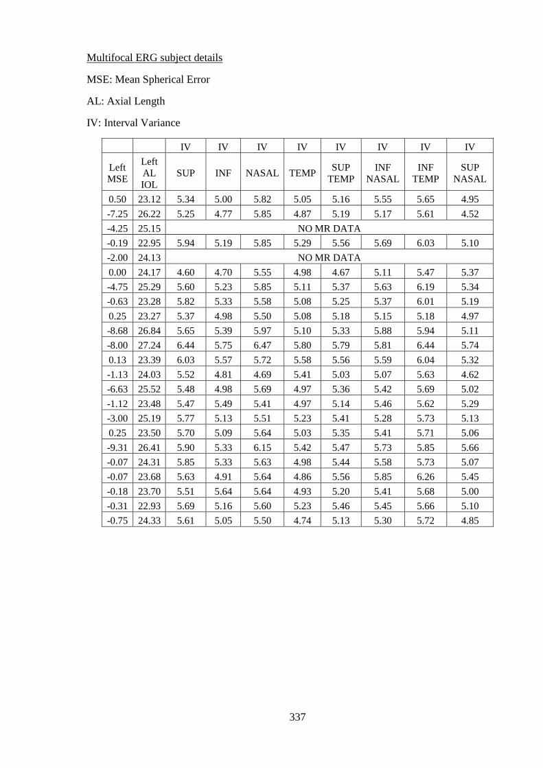
337

Multifocal ERG subject details

MSE: Mean Spherical Error

AL: Axial Length

IV: Interval Variance

IV IV IV IV IV IV IV IV

Left

MSE

Left

AL

IOL

SUP INF NASAL TEMP SUP

TEMP

INF

NASAL

INF

TEMP

SUP

NASAL

0.50 23.12 5.34 5.00 5.82 5.05 5.16 5.55 5.65 4.95

-7.25 26.22 5.25 4.77 5.85 4.87 5.19 5.17 5.61 4.52

-4.25 25.15 NO MR DATA

-0.19 22.95 5.94 5.19 5.85 5.29 5.56 5.69 6.03 5.10

-2.00 24.13 NO MR DATA

0.00 24.17 4.60 4.70 5.55 4.98 4.67 5.11 5.47 5.37

-4.75 25.29 5.60 5.23 5.85 5.11 5.37 5.63 6.19 5.34

-0.63 23.28 5.82 5.33 5.58 5.08 5.25 5.37 6.01 5.19

0.25 23.27 5.37 4.98 5.50 5.08 5.18 5.15 5.18 4.97

-8.68 26.84 5.65 5.39 5.97 5.10 5.33 5.88 5.94 5.11

-8.00 27.24 6.44 5.75 6.47 5.80 5.79 5.81 6.44 5.74

0.13 23.39 6.03 5.57 5.72 5.58 5.56 5.59 6.04 5.32

-1.13 24.03 5.52 4.81 4.69 5.41 5.03 5.07 5.63 4.62

-6.63 25.52 5.48 4.98 5.69 4.97 5.36 5.42 5.69 5.02

-1.12 23.48 5.47 5.49 5.41 4.97 5.14 5.46 5.62 5.29

-3.00 25.19 5.77 5.13 5.51 5.23 5.41 5.28 5.73 5.13

0.25 23.50 5.70 5.09 5.64 5.03 5.35 5.41 5.71 5.06

-9.31 26.41 5.90 5.33 6.15 5.42 5.47 5.73 5.85 5.66

-0.07 24.31 5.85 5.33 5.63 4.98 5.44 5.58 5.73 5.07

-0.07 23.68 5.63 4.91 5.64 4.86 5.56 5.85 6.26 5.45

-0.18 23.70 5.51 5.64 5.64 4.93 5.20 5.41 5.68 5.00

-0.31 22.93 5.69 5.16 5.60 5.23 5.46 5.45 5.66 5.10

-0.75 24.33 5.61 5.05 5.50 4.74 5.13 5.30 5.72 4.85

338

SURFACE AREAS FOR MFERG SUBJECTS

XQ DATA

SURFACE AREAS IN mm²

MSE (D) SUP INF NASAL TEMP

0.495 220.5121 231.6063 212.0273 247.1733

-7.25 240.2087 218.6113 203.9558 245.1092

-4.25 NO MR DATA

-0.185 228.5753 220.6947 228.6536 234.2750

-1.995 NO MR DATA

0 215.7808 227.5891 264.7641 243.9464

-4.75 257.6212 270.3276 273.6055 232.1776

-0.625 224.7261 235.0683 213.6098 227.5266

0.245 211.4910 220.7778 227.8496 204.4018

-8.68 271.8368 292.8415 283.6517 261.6697

-8 308.1347 285.7326 332.4242 309.9796

0.125 262.6133 240.4372 240.4700 231.6088

-1.125 206.7012 214.7728 182.7880 193.3873

-6.625 205.9602 242.8201 239.5309 220.4595

-1.12 230.0244 212.9193 214.0497 200.1824

-3 247.8121 229.8404 222.9243 249.7332

0.245 212.6054 214.0648 192.8345 232.4840

-9.31 237.9476 260.4218 253.1010 277.5386

-0.065 239.3049 261.9538 218.0068 237.9423

-0.065 231.7679 253.4496 213.3948 232.7510

-0.18 224.2802 245.0085 196.0024 213.2033

-0.31 210.4789 229.4705 210.4921 229.4853

-0.75 207.6813 226.3243 200.2533 217.9766

339

SURFACE AREAS FOR MFERG SUBJECTS

+Q DATA

SURFACE AREAS IN mm²

MSE (D) SUP TEMP INF NASAL INF TEMP SUP NASAL

0.495 228.995 220.893 201.993 219.931

-7.25 230.640 205.276 204.889 228.456

-4.25 NO MR DATA

-0.185 241.470 223.376 229.823 227.686

-1.995 NO MR DATA

0 199.886 240.797 222.870 229.002

-4.75 239.939 274.079 282.777 249.885

-0.625 227.165 223.032 381.416 444.166

0.245 201.977 224.117 190.752 196.597

-8.68 274.048 290.478 262.627 283.142

-8 249.129 325.232 257.585 296.791

0.125 236.829 223.005 221.415 217.222

-1.125 238.315 270.037 195.226 203.463

-6.625 220.628 259.240 235.684 231.237

-1.12 208.042 205.342 207.681 242.480

-3 246.462 230.063 232.114 239.774

0.245 228.247 198.569 202.867 219.340

-9.31 292.378 299.246 278.918 309.175

-0.065 260.664 263.864 239.597 222.162

-0.065 265.579 229.875 240.530 263.464

-0.18 235.572 206.517 246.863 207.394

-0.31 214.238 204.062 220.660 231.870

-0.75 214.077 204.062 205.702 208.842

340

APPENDIX 10: GANGLION CELL DENSITY: DETECTION TASK DATA


Spatial Frequency

c/deg Subject a Subject b

1 98 100

2 100 96

3 86.67 88

4 76 81.33

5 69.33 84

6 45.33 52

7

48


Spatial Frequency

c/deg Subject c Subject d

1 88 98

2 82 92

3 82 72

3.5

68

4 60 50

5 54 42

6 54

7 46

341

APPENDIX 11: GANGLION CELL DENSITY: DIRECTION DISCRIMINATION TASK

DATA


Spatial Frequency

c/deg Subject a Subject b

1 100 100

2 98 96

3 70 64

3.5 68 52

4 56 57.33

5 48 56

6

48


Spatial Frequency

c/deg Subject c Subject d

1 98.67 64.33

2 72 58

2.5

50.17

3 50 41

3.5 46

4 54.67 26.67

5

39

342

Ganglion cell Density: Case Study R.C raw data

Detection

Spatial frequency c/deg Right eye % correct Left eye % correct

1 96 100

2 88 84

3 76 100

4 56 80

4.5 84

5 52 56

5.5 56

6 58 56

6.5 56

Direction discrimination

Spatial frequency c/deg Right eye % correct Left eye % correct

1 92 96

1.5 64 88

2 48 38

2.5 40 68

research.aston.ac.uk · 2017-02-06 · 3 acknowledgements . i would like to begin by thanking my...

Documents