˘ ˇ - aalborg universitetkom.aau.dk/group/05gr892/files/sipcom8_improving gsm receiver.pdf ·...
TRANSCRIPT

������������ ����������������������� ���!�"��$#&%�'������'�()�+*$��,�.-/�����0�1��2��3-4-5���!��6�6�7���8�9����6�$���� :�����
;=<?>A@B<DCFEHG,IKJL>�<NM7OP>QJ7RTSVU�W.XLY=Z[Z�\^]PIA_ `Ba�<Qb�c�MQd e7>f_g>�h=i�a�j[>'k=l�m^Y=n'o�mHp[R^\=\
Improving GSM Receiverby using
It era t ive E q u a l iz a t ion a nd D ecod ing%rqts02u�8- v0wx� �y��*5z${�| %3*$�}�����"|�~0~��p:dDi6MK>��>AM?d?>�<


Aalborg UniversityThe Faculty of Engineering and ScienceDepartment of Communication Technology
Fredrik Bajers Vej 7 DK-9220 Aalborg Øst Telephone +45 96 35 87 00
Title: Improving GSM Receiver by using Iterative Equalization and DecodingTheme: Methods and AlgorithmsProject period: February 1 - May 30, 2005Specialization: Signal and Information Processing in Communications
Project group:
892
Group members:
Kim Nørmark
Ole Lodahl Mikkelsen
Supervisor:
Bin Hu
Johan Brøndum
Romain Piton
Publications: 7
Pages:Report 64Appendix 19
Abstract
This report documents the design of an improved re-ceiver for a GSM system. The receiver utilizes iter-ative equalization and decoding.The system model consists of a modified GSMtransmitter, a channel model, and a modified GSMreceiver. The transmitter consists of a (23,33) convo-lutional encoder, a block interleaver, and a discretetime BPSK modulator. The channel is modelled asa multipath quasi-static block fading channel anda matched filter. The receiver consists of a Max-log-MAP equalizer, a deinterleaver, and a Max-log-MAP decoder implemented in an iterative manner.Simulation and results show that there is a perfor-mance gain of 0.7 dB for BER at 10−3 by usingiterative equalization and decoding for the first it-eration. The following iterations do not give anyappreciable performance gain. If fading is not pro-duced due to multipath propagation in the channel,no irrecoverable bursts will occur and then there isa performance gain for each new iteration up till thefourth iteration. If the interleaver size is increasedfrom 456 bits to 4104 bits, there is only little perfor-mance gain compared to size 456 bits at higher SNRand for the first iteration.


Preface
This report is conducted by group 892 of the Signal and Information Processing in Communi-cations (SIPCom) specialization, 8th semester, Aalborg University. The project period spannedfrom february 1 to may 30, 2005, and the topic was "Improving GSM Receiver by using IterativeEqualization and Decoding" under the theme "Methods and Algorithms".
The group has in the project implemented a modified GSM transmitter, a channel model, and amodified GSM receiver. The receiver was improved by using an iterative technique.
This report is a documentation of the considerations made during this period. Furthermore, itdocuments the design of the considered system model and the simulations and results conducted.
The motivation for this project and for the considered system model is stated in the first chapter,the Introduction. Also the structure of this report is stated in the end of the Introduction.
An appendix are accompanying the report, concerning the implementation of the system model.
A CD is attached to the report. On the CD is the MatLab source code available, and also a ps fileand a pdf file of the report is available.
—————————————- —————————————-
Kim Nørmark Ole Lodahl Mikkelsen
III

Contents
1 Introduction 11.1 Digital Communication Systems . . . . . . . . . . . . . . . . . . . . . . . . . . 21.2 GSM Systems . . . . . . . . . . . . . . . . . . . . . . . . . . . . . . . . . . . . 31.3 The System Model . . . . . . . . . . . . . . . . . . . . . . . . . . . . . . . . . 7
2 Channel Model 132.1 The AWGN Channel . . . . . . . . . . . . . . . . . . . . . . . . . . . . . . . . 132.2 The Multipath Fading Channel . . . . . . . . . . . . . . . . . . . . . . . . . . . 152.3 The Matched Filter . . . . . . . . . . . . . . . . . . . . . . . . . . . . . . . . . 18
3 Modulation 223.1 Gram-Schmidt Orthogonalization Procedure . . . . . . . . . . . . . . . . . . . . 233.2 Binary Phase Shift Keying . . . . . . . . . . . . . . . . . . . . . . . . . . . . . 24
4 Convolutional Encoding 304.1 The Convolutional Encoder . . . . . . . . . . . . . . . . . . . . . . . . . . . . . 304.2 Properties of Convolutional Codes . . . . . . . . . . . . . . . . . . . . . . . . . 32
5 Convolutional Decoding using the Viterbi Algorithm 355.1 Maximum Conditional Probability . . . . . . . . . . . . . . . . . . . . . . . . . 355.2 Optimal Path Through the Trellis . . . . . . . . . . . . . . . . . . . . . . . . . . 365.3 Performance . . . . . . . . . . . . . . . . . . . . . . . . . . . . . . . . . . . . . 38
6 Equalization 406.1 Signal Model . . . . . . . . . . . . . . . . . . . . . . . . . . . . . . . . . . . . 406.2 Maximum-Likelihood Sequence Detection . . . . . . . . . . . . . . . . . . . . . 436.3 Viterbi Equalizer . . . . . . . . . . . . . . . . . . . . . . . . . . . . . . . . . . 446.4 Max-log-MAP Equalizer . . . . . . . . . . . . . . . . . . . . . . . . . . . . . . 456.5 Performance . . . . . . . . . . . . . . . . . . . . . . . . . . . . . . . . . . . . . 48
7 Iterative Equalization and Decoding 507.1 The Non-Iterative Receiver . . . . . . . . . . . . . . . . . . . . . . . . . . . . . 507.2 Turbo Decoding . . . . . . . . . . . . . . . . . . . . . . . . . . . . . . . . . . . 517.3 Iterative Equalization and Decoding . . . . . . . . . . . . . . . . . . . . . . . . 537.4 Simulations and Results . . . . . . . . . . . . . . . . . . . . . . . . . . . . . . . 56
8 Conclusion 61
IV
CONTENTS
Appendix 65
A Implementation 65A.1 (23,33) Convolutional Encoder . . . . . . . . . . . . . . . . . . . . . . . . . . . 66A.2 Interleaver . . . . . . . . . . . . . . . . . . . . . . . . . . . . . . . . . . . . . . 67A.3 BPSK Modulator . . . . . . . . . . . . . . . . . . . . . . . . . . . . . . . . . . 68A.4 4-Paths Quasi-static Block Fading Channel . . . . . . . . . . . . . . . . . . . . 70A.5 Equalizer . . . . . . . . . . . . . . . . . . . . . . . . . . . . . . . . . . . . . . 72A.6 Deinterleaver . . . . . . . . . . . . . . . . . . . . . . . . . . . . . . . . . . . . 74A.7 Max-log-MAP Decoder . . . . . . . . . . . . . . . . . . . . . . . . . . . . . . . 75
Bibliography 83
V


CHAPTER
Introduction 1There has been a growing use of digital communication systems over the last five decades, andmany applications today have a need for reliable and fast transmission through a channel. A fewexamples of applications could be systems for transmission of voice-, image-, or TV-signals, whichwe know and use in our daily life, and examples of channels could be wirelines for telephony orinternet connections, fiber optic cables for music or video transmission, or the atmosphere forwireless transmission.
The basic idea with digital communication systems is to transmit a binary information sequencethrough a channel, and then receive it with as little error probability as possible. In order to dothat, much signal processing is needed, both to transmit the information through the channel, and toprotect the transmitted information to prevent errors in the estimated binary information sequencerecovered from the received channel corrupted signal.
A digital communication system used for mobile telephony is the Global System for Mobile Com-munications (GSM), which is the most popular standard for mobile phones today. The GSMsystem transmits the digital information through the atmosphere by conveying the information toan analog waveform.
Since the GSM standard was introduced in 1982, there has been a major development in the field ofdigital communications design, and the requirements for the data transmission rate has increased.New methods for achieving better performance are needed, and the aim of this project is to improvethe receiver part of a GSM system model. An often used process in GSM systems is a sequentialequalization and decoding process, and a method to improve the performance of this process is touse an iterative technique, where the equalizer and the decoder are exchanging information witheach other in an iterative manner.
To give a general understanding of how digital communication systems works, we will give a shortintroduction to digital communication systems in the first section of this chapter. The next sectionwill give a short introduction to the GSM system with emphasize on the coding part, and in thethird and last section of the chapter, we will discuss the implemented system model and state theassumptions and constraints we have made in the project.
The reference for this chapter is [Proakis et al., 2002] unless any other is specified.
1

CHAPTER 1. INTRODUCTION
1.1 Digital Communication Systems
The digital communication system consists of a transmitter and a receiver. In the transmitter, thebinary information sequence in transformed into an electrical signal called the message signal,and the message signal is mapped into a carrier waveform suitable for transmission through thechannel by a process called modulation. The modulated carrier waveform is transmitted throughthe channel and received in a degraded version by the receiver. In the receiver, the message signalis recovered from the received carrier waveform by a process called demodulation. Moreover, thereceiver also performs amplification of the received signal, low pass filtering, analog-to-digitalconversion (ADC), sampling, and noise suppression. In the front end of the receiver, some ad-ditive noise called thermal noise corrupts the transmitted signal in a random manner due to theamplification, which the system has to deal with.
The channel is the physical medium that is used to send the carrier waveform from the transmitterto the receiver. An essential feature of the channel is that it corrupts the transmitted signal due toman-made noise, interference from other users of the channel, and for wireless communicationsalso from atmospheric noise picked up by the receiving antenna. In wireless channels, the phe-nomenon called fading may occur due to multipass propagation. It is a distortion of the transmittedsignal and is characterized as a time variant amplification of the amplitude. The affect of all thesecorruptions and distortions must be taken into account in the design of the digital communicationsystem.
So far we have described some of the transmitter, the channel, and the receiver. If we disregard thetransmitting and receiving antennas, and the amplification, filtering, ADC, sampling, and noisesuppression, the transmitter is basically just a modulator and the receiver is basically just a de-modulator. The modulator maps a discrete (or digital) information sequence onto an analog carrierwaveform, which is transmitted through the analog channel. The demodulator recovers the discreteinformation sequence by mapping the received analog carrier waveform into a discrete sequence.Digital communication systems often consists of more than a modulator and a demodulator, and ablock diagram of the basic elements of a digital communication system is shown in figure 1.1.
����������������� ������ � ���������� ��
������������
� ���� ���������� ���������������� �� ������
! "$# %�&�%(' )
* + , - .0/1, 23)- "$# %�&�%$' )
4 %()52�&�%(' )
6�7 + 23' 8923): %()$2�&�%(' )
;� ����<� ������ ������
= ��>�������$���?<����� ���
; ����$� ���� � ������
@A����>�������$���?<����� ���
Figure 1.1: Basic elements of a digital communication system.
It is desirable to express the information with as few bits as possible in order to achieve fast datatransmission. Therefore, instead of transmitting raw data from e.g. a speech signal or a videosignal, a source encoding process is applied. In the receiver, a corresponding source decodingprocess is applied to re-create the raw data before the output transducer.
2

1.2. GSM SYSTEMS
One of the most important properties of a digital communication system is to recover the originaldiscrete information sequence with as few errors as possible. By using a channel encoding process,some redundancy bits are added to the discrete information sequence in a controlled manner. Theinput to the encoder is denoted as the info word, and the output is denoted as the code word. In thereceiver, a corresponding channel decoding process is applied to re-create an estimated info wordfrom the observed code word.
The channel coding gives an increased reliability of the received data and improves the fidelity ofthe received signal, but it also increases the number of transmitted bits per time instant and therebythe data transmission rate requirement. Also the modulation scheme chosen has effect on both thedata transmission rate and the error probability, and the different modulation schemes are more orless suitable for different channels. These issues are a trade off the designer must have in mindwhen designing a digital communication system.
1.2 GSM Systems
The GSM standard for digital communication has been developed by ETSI1 Special Mobile Group(SMG) since 1982. The group was first known as "Groupe Special Mobile", which was created byCEPT2. Groupe Special Mobile was transferred from CEPT to ETSI in 1992 and was renamed toETSI SMG, and today the GSM standard is used by 254 million subscribers world-wide in over142 countries around the world. [ETSI, 2004]
The GSM system is a digital cellular communication system that uses Time-Division Multiple Ac-cess (TDMA) to accommodate multiple users. European GSM systems uses the frequency bands890-915 MHz and 935-960 MHz for uplink and downlink respectively, and each band is dividedinto 125 channels with a bandwidth of 200 kHz. Each of the 125 channels can accommodate 8users by creating 8 TDMA non-overlapping time-slots of 576.92 µs, and 156.25 bits are transmit-ted in each time-slot with the structure denoted in figure 1.2. The data transmission rate is 156.25 bits
576.92µs= 270.83 kbps.
��� ��� ��� ����� �� �
���� ���� � � ��� ������ � ��� ������� � ��� ���� � �
��� ��� ���� � � !� ��� "#� "#�$��� � � %'&# )(� *� "+ &�-,.�� � &#"$��� � �%'&# #( /� "+-&#� ,/��� � &"0��� � �
Figure 1.2: Time-slot structure for 1 user.
A block diagram of a GSM system is shown in figure 1.3. It consists of the same blocks as theblock diagram for a general structure of a digital communication system shown in figure 1.1, butit also consists of more blocks to ensure proper and reliable transmission.
The RPE-LPC speech coder and the Speech synthesizer is the source coding/decoding part. Theanalog speech signal is in the RPE-LPC speech coder mapped into digital Linear Predictive Coding(LPC) coefficients by using the Residual Pulse-Excited (RPE) technique. In the Speech synthe-sizer, an estimation of the analog speech signal is constructed.
1European Telecommunications Standards Institute2European Conference of Postal and Telecommunications
3

CHAPTER 1. INTRODUCTION
������� ������� � ���������� ��
�������� �� � � � � ��� ���
��! ������ "� ��� ������ ���
# �� �$�%� ���� & &���� �� ��� '� ��
( �� � ���� &)��� �� ��� '� ��
�������� ���� ������� �� *�+ , -�. + / 0 +�1 2�+ /
�������� �� �$�%���� � '� ��
3 ��� ���� ��4 � � � ��
��� 4 � � � ���56879 �����: % 4 4 ��
�������� ��
��! ������ "� ��� ������ ���
# �� �$�%� ���� &��������� ��" &���� �� ��� '� ��
;<3=(�>�?����%�� ��� ���
@�793A6� %�� � � ��� �B� ��
C %��DE����� �� : � ��F ��� ���� ���G� �� �������� ��
��������� ��
HJI�K L M�NO P�Q�Q�R S8O T N�I�K�L
U O V T W K V Q�XK I�K�L M�N
O P�Q�Q�R S8O T N�I�K�L
Figure 1.3: Block diagram of a GSM system.
The Channel encoder and the Channel decoder is the channel coding part. The channel encoderadds redundancy to the signal with linear convolutional block encoding, and the channel decoderdecodes each block.
Linear convolutional block codes are designed to correct random errors, but in most physicalchannels the assumption that the noise appears randomly and independently is not valid. Often theerrors tend to occur in bursts, and an effective method for correction of error bursts is to interleavethe coded data. In this way the location of the errors appear randomly and is distributed overseveral code words rather than one. The Interleaver and the Deinterleaver is the interleaving part,which is not a part of figure 1.1.
The Burst assembler organizes the interleaved coded information bits for burst transmission car-rying both the coded information bits and a "training sequence" to enable the receiver to estimatethe characteristics of the channel.
The TDMA multiplexer distributes the bursts for the eight time-slots in the channel.
The GMSK modulator modulates the digital information onto an analog carrier waveform withGaussian Minimum-Shift Keying (GMSK) technique.
In the Frequency hopping synthesizer, the analog carrier waveform is hopped to different frequen-cies controlled by the PN code generator, and the received signal is dehopped and translated tobaseband by the Frequency synthesizer.
The Lowpass filter, ADC, and buffer is a part of the demodulator in figure 1.1. The signal is hereconverted to discrete time.
4
1.2. GSM SYSTEMS
The Channel estimator uses the training sequence in the received bursts to estimate the charac-teristics of the channel for each time-slot and sends the coefficients to the matched filter and thechannel equalizer.
The Matched filter seeks to maximize the SNR of the channel corrupted signal to suppress thenoise.
The Channel equalizer uses Maximum Likelihood (ML) sequence detection to estimate the mostlikely interleaved code word.
1.2.1 The GSM Standard: Coding
The GSM standard defined in [3GPP, 2004] states that the input to the channel encoder is a datasequence, denoted as d, of 260 information (or info) bits. The elements in d are denoted as dkand represent the LPC coefficients arranged after importance, where d1 is most important and d260
is least important. The 182 first bits are protected by parity bits and are called class 1, and thefollowing 78 bits, called class 2, are unprotected.
Reordering of Class 1 Information Bits
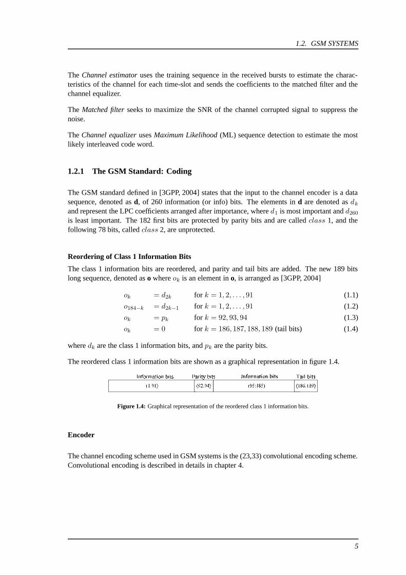
The class 1 information bits are reordered, and parity and tail bits are added. The new 189 bitslong sequence, denoted as o where ok is an element in o, is arranged as [3GPP, 2004]
ok = d2k for k = 1, 2, . . . , 91 (1.1)
o184−k = d2k−1 for k = 1, 2, . . . , 91 (1.2)
ok = pk for k = 92, 93, 94 (1.3)
ok = 0 for k = 186, 187, 188, 189 (tail bits) (1.4)
where dk are the class 1 information bits, and pk are the parity bits.
The reordered class 1 information bits are shown as a graphical representation in figure 1.4.
����� ����� ����� �� ��������� ����� ���� ���� �� ����
���������� "!�#$���&%'$ #�( ���)������ "!�#$*���+%�$ #�(,-!���$ # .+%'$ #/( 01!�$ 2)%'$ #/(
Figure 1.4: Graphical representation of the reordered class 1 information bits.
Encoder
The channel encoding scheme used in GSM systems is the (23,33) convolutional encoding scheme.Convolutional encoding is described in details in chapter 4.
5

CHAPTER 1. INTRODUCTION
The 189 reordered class 1 bits are encoded with a convolutional encoder with code rate Rc = 1/2and defined by the polynomials:
g1 = 1 +D3 +D4 (1.5)
g2 = 1 +D +D3 +D4 (1.6)
which gives the (23,33) encoding scheme. 23 is the octal value of g1, and 33 is the octal value ofg2.
The 189 class 1 bits give a sequence of 378 bits when encoded. The 78 uncoded class 2 bits areadded to the 378 coded class 1 bits, which gives a code word sequence, denoted as c, of 378 + 78bits = 456 bits. This is shown in figure 1.5 as a graphical representation. [3GPP, 2004]
����� ����� ������ �� ��������������������� �"!$# !�!�%&��'�(")$'�� *,+.-�'�($���0/�($��',1,/�1 ���������&�2��($'�+3/�($��',1"/�1
Figure 1.5: Graphical representation of the code word.
Decoder
The GSM standard does not specify any decoding algorithm, but an often used decoder in theGSM system is a ML decoder based on the Viterbi Algorithm. Convolutional decoding with theViterbi Algorithm is described in details in chapter 5.
1.2.2 The GSM Standard: Interleaving
When the 456 coded bits are transmitted through the channel, they are block interleaved. Theresult of the interleaving is a distribution of the 456 code bits over 8 blocks of 114 bits, where theeven numbered bits are in the first 4 blocks, and the odd numbered bits are in the last 4 blocks.Each interleaver block is transmitted as 2 half bursts, where each half burst consists of 57 bits.[3GPP, 2004]
The algorithm for the GSM interleaver is defined as [3GPP, 2004]
IB,j = cm,k for k = 1, 2, . . . , 456 (1.7)
where
m = 1, 2, . . . (1.8)
B = B0 + 4m+ ([k − 1] mod 8) (1.9)
j = 2[(49[k − 1]) mod 57] + [([k − 1] mod 8) div 4] (1.10)
where IB,j is a bit in a interleaver block, B is the burst number, and j is the bit number in burst B.m is the code word number, and k is the bit number in code word m.
One coded block is interleaved over 8 bursts starting from B0. The next coded block is alsointerleaved over 8 bursts but starting from B0 + 4.
6
1.3. THE SYSTEM MODEL
1.2.3 The GSM Standard: Mapping in Bursts
Each burst consists of 2 half bursts of 57 bits and 2 flag bits indicating the status of even/odd num-bered bits. The burst is transmitted in one time-slot in a channel for one user with the structuredepicted in figure 1.2.
The mapping of the bursts is defined as:
eB,j = IB,j for j = 1, 2, . . . , 57 (1.11)
eB,59+j = IB,57+j for j = 1, 2, . . . , 57 (1.12)
eB,58 = hlB (1.13)
eB,59 = huB (1.14)
where hlB and huB are the flag bits for the B’s burst.
1.3 The System Model
This section describes the system model considered in this project. We will go through somedesign considerations and focus on the assumptions and the constraints made in the project.
1.3.1 Channel Model Design
Mathematical Model
In the design of communication systems for transmission through a physical channel, it is impor-tant to have a good mathematical channel model that reflects the most important characteristics ofthe physical channel.
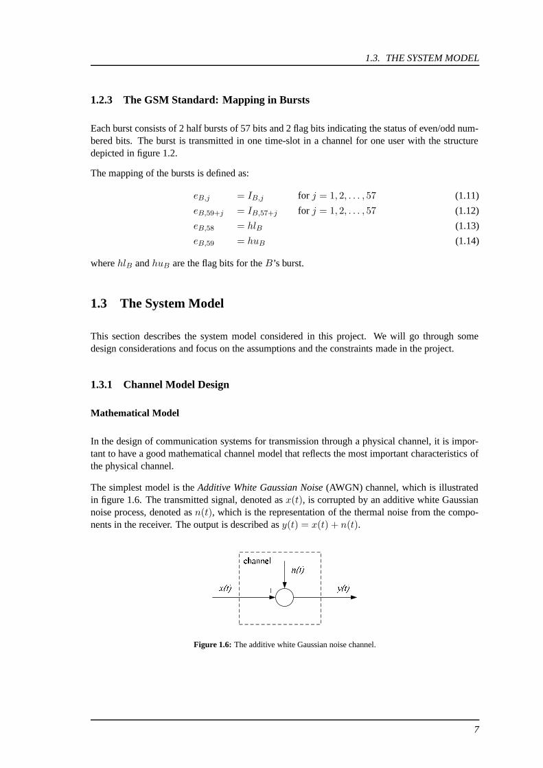
The simplest model is the Additive White Gaussian Noise (AWGN) channel, which is illustratedin figure 1.6. The transmitted signal, denoted as x(t), is corrupted by an additive white Gaussiannoise process, denoted as n(t), which is the representation of the thermal noise from the compo-nents in the receiver. The output is described as y(t) = x(t) + n(t).
����� � ����� �
��� ��� ����������
��
Figure 1.6: The additive white Gaussian noise channel.
7

CHAPTER 1. INTRODUCTION
Attenuation is often incorporated in the channel model, and the expression for the output is simply
y(t) = a · x(t) + n(t) (1.15)
where a is the attenuation factor. For a = 1 we have the AWGN channel, otherwise it is called afading channel.
For some channels, it is important that the transmitted signal does not exceed a specified bandwidthlimitation. Such a channel can be characterized as a time-invariant linear filter as depicted in figure1.7. The channel output for such a channel is described as
y(t) = x(t) ∗ a(t) + n(t) (1.16)
=
∫ ∞
−∞a(τ)x(t− τ) dτ + n(t) (1.17)
where a(t) is the impulse response of the linear filter, and * denotes a convolution in time.
����� � ����� �
��� �� ��� �������
����� �
��
Figure 1.7: The linear filter channel with additive noise.
A third channel model is the linear time-variant filter channel, where the characteristics are time-variant due to time-variant multipath propagation of the transmitted signal. The impulse responseof the filter is described as
a(t) =L∑
i=1
ai(t)δ(t− τi) (1.18)
where the ai(t)’s represent the time-variant attenuation factors for the L multipath propagationpaths, and the τi’s are the time-delays for the ai(t)’s.
The channel output of the linear time-variant filter channel is described as
y(t) =L∑
i=1
ai(t)x(t− τi) + n(t) (1.19)
The affect of multipath propagation is a phenomenon called InterSymbol Interference (ISI). Thisissue is described in chapter 2.
The Sampling Process
In a physical channel, the digital data is transmitted by an analog carrier waveform, and the re-ceived waveform is demodulated to recover the analog message signal. The message signal is then
8

1.3. THE SYSTEM MODEL
low pass filtered to remove irrelevant frequencies, sampled to represent it in discrete time, andquantized by an ADC to represent it as discrete values.
The sampling process converts the received analog signal into a corresponding sequence of sam-ples that are uniformly spaced in time. If we consider an analog signal, denoted as y(t), offinite energy and specified at all time, the sampling process of the signal can be described as[Haykin, 2001]
yδ(t) =∞∑
k=−∞y(kTs) δ(t− kTs) (1.20)
where Ts is the sampling time, yδ(t) is the sampled signal of y(t), and δ(t) is the delta functionwhere δ(t) = 1 for t = 0 and δ(t) = 0 otherwise.
By expressing equation 1.20 in the frequency domain, the Fourier transform of yδ(t) can be ex-pressed as
Yδ(f) =∞∑
k=−∞y(kTs) e
−j2πkfTs (1.21)
and by assuming that y(t) is bandlimited and has no frequency components for f > W Hz, whereW is called the bandwidth of the signal, Yδ(f) may by choosing Ts = 1
2W be rewritten as
Yδ(f) =
∞∑
k=−∞y
(k
2W
)e
−jπkfW (1.22)
The spectrum of Yδ(f) is shown in figure 1.8, where fs = 1Ts
is the sampling rate.
�������
�
� � � � � � � � ���
Figure 1.8: Spectrum of Yδ(f) for Ts = 12W
.
By inspecting figure 1.8 it is clear that if fs < 2W , the triangles will overlap. This will produce theunwanted phenomenon called aliasing. To avoid aliasing, the sampling rate must be greater thanor equal to the so-called Nyquist rate (fs ≥ 2W ). [Haykin, 2001]
Aliasing is a phenomenon considered in the frequency domain. The corresponding phenomenonin the time domain is ISI.
Channel Capacity
The bandwidth of the channel defines the limit for reliable data transmission through a channel,and the term reliable transmission, defined by Shannon in 1948, describes when it is theoreticalpossible to achieve error free transmission by appropriate coding. The channel capacity can be
9
CHAPTER 1. INTRODUCTION
expressed as
C = W log2
(1 +
PsWN0
)[ bits/s ] (1.23)
where W is the channel bandwidth, Ps is the signal power constraint, and N0 is the power spectraldensity of additive noise associated with the channel. Reliable transmission is achievable whenthe data transmission rate is less than the channel capacity.
By increasing the channel bandwidth, the channel capacity will increase also, but there is a limitfor the capacity for a given channel, and this limit is called the Shannon limit. It is desired to get asclose to the Shannon limit as possible to achieve the maximum performance for a given channel.
1.3.2 Assumptions and Constraints
The aim (or main scope) of this project is to improve the receiver in a GSM system model by usingiterative equalization and decoding, but due to the time constraint in the project and to the fact thatnot all blocks are of equal relevancy, we will not implement a complete GSM system model.
The following elements has been disregarded compared to the GSM system depicted in figure 1.3:
Source Coding: Speech coding has only little relevance to the main scope, thus the RPE-LPCspeech coder and the Speech synthesizer will not be implemented.
Multiuser System: Since the multiuser aspect is not in the scope of this project, the TDMA mul-tiplexer and the frequency hopping will not be implemented.
GMSK Modulation: The modulation process is used to transmit the digital information throughthe channel and can not be omitted, but due to the time constraint, we will consider a simplermodulation process, namely the Binary Phase Shift Keying (BPSK) modulation.
Continuous Time Bandpass Transmission: A BPSK modulated signal is an analog carrier wave-form where the digital information is conveyed by the phase. We consider a digital commu-nication system with emphasis on the coding part and not on the modulation part, and wewill therefore only consider a representation of BPSK modulation in a digital environment.
Channel Estimation: Due to the time constraint, the channel estimator will not be implemented.In stead we assume to have perfect knowledge of the channel at all time.
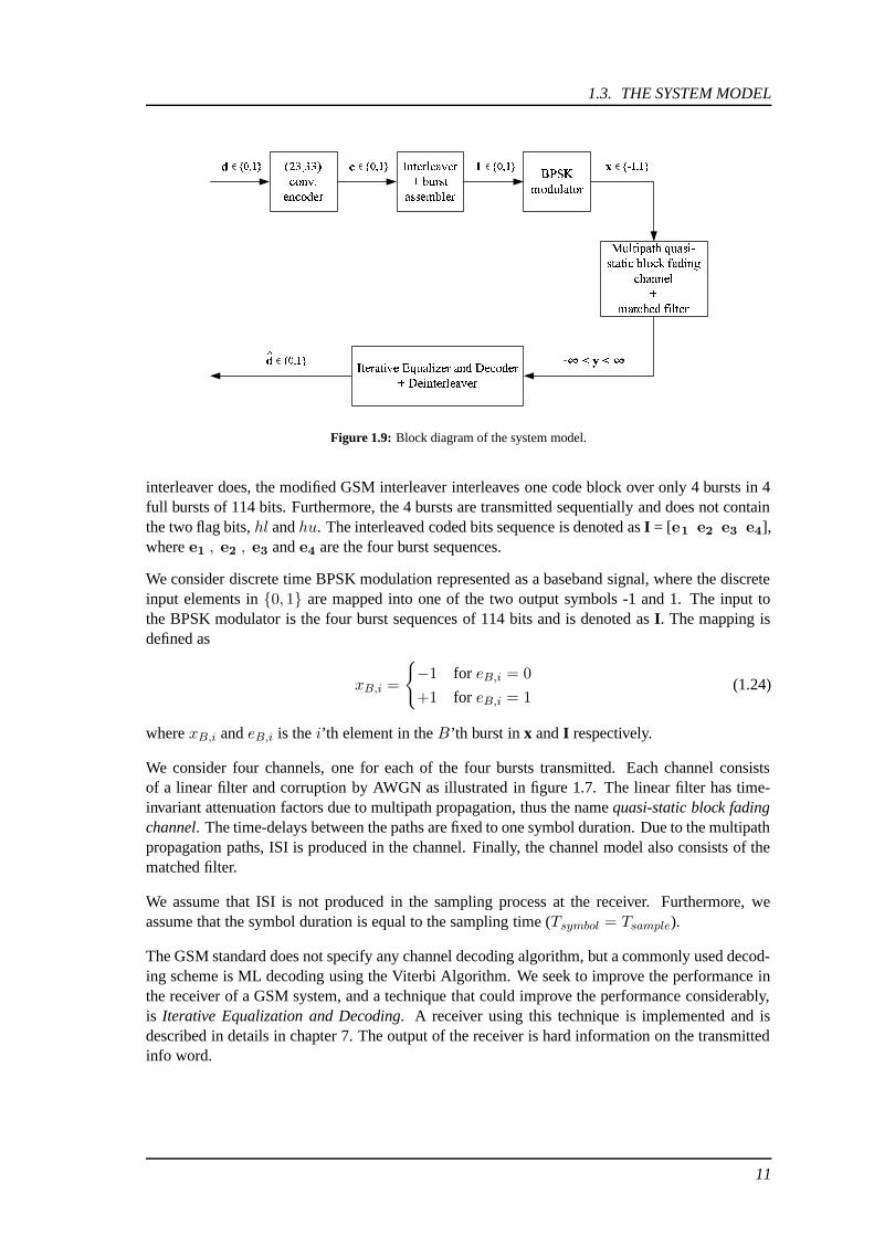
This project will consider the blocks depicted in figure 1.9, where we assume that the input to thesystem model is a discrete information sequence generated by a random generator. This sequenceis also called the info word and is denoted as d. The following channel encoder is implemented asa (23,33) convolutional encoder, and where the GSM standard defines 182 class 1 bits and 78 class2 bits in the info word, and only encodes the class 1 bits + parity and tail bits, the implementedencoder in the system model encodes a info word of 224 bits + 4 tail bits. The output sequence of456 bits is called the code word and is denoted as c.
The code word is input to the Interleaver + burst assembler, where the code word is block inter-leaved with a modified GSM interleaver and mapped into four bursts per transmission. In steadof interleaving one coded block of 456 bits over 8 bursts in 16 half bursts of 57 bits as the GSM
10
1.3. THE SYSTEM MODEL
������� ��������� �������������
� �������������� �������� �"!#�
��!$!"��% � �����
&('*)�+%��� ���,�-��
. / 0 1
24352. 6 � �-���"�,�87 ��(9(: ���;7;<����=�,���?>@���������� >@��7;���-���A�����, ����
B � �87;C��,�8DE: ��!#7-F!-���$�87- � ����G?HI����7;��J
�D�����������
%4�,�-�D����?H#7 � �-���
K#L�M;N$O K"L�M;N$OK"L�M;N$O KIPAN"M N$O
K#L�M N,O
Figure 1.9: Block diagram of the system model.
interleaver does, the modified GSM interleaver interleaves one code block over only 4 bursts in 4full bursts of 114 bits. Furthermore, the 4 bursts are transmitted sequentially and does not containthe two flag bits, hl and hu. The interleaved coded bits sequence is denoted as I = [e1 e2 e3 e4],where e1 , e2 , e3 and e4 are the four burst sequences.
We consider discrete time BPSK modulation represented as a baseband signal, where the discreteinput elements in {0, 1} are mapped into one of the two output symbols -1 and 1. The input tothe BPSK modulator is the four burst sequences of 114 bits and is denoted as I. The mapping isdefined as
xB,i =
{−1 for eB,i = 0
+1 for eB,i = 1(1.24)
where xB,i and eB,i is the i’th element in the B’th burst in x and I respectively.
We consider four channels, one for each of the four bursts transmitted. Each channel consistsof a linear filter and corruption by AWGN as illustrated in figure 1.7. The linear filter has time-invariant attenuation factors due to multipath propagation, thus the name quasi-static block fadingchannel. The time-delays between the paths are fixed to one symbol duration. Due to the multipathpropagation paths, ISI is produced in the channel. Finally, the channel model also consists of thematched filter.
We assume that ISI is not produced in the sampling process at the receiver. Furthermore, weassume that the symbol duration is equal to the sampling time (Tsymbol = Tsample).
The GSM standard does not specify any channel decoding algorithm, but a commonly used decod-ing scheme is ML decoding using the Viterbi Algorithm. We seek to improve the performance inthe receiver of a GSM system, and a technique that could improve the performance considerably,is Iterative Equalization and Decoding. A receiver using this technique is implemented and isdescribed in details in chapter 7. The output of the receiver is hard information on the transmittedinfo word.
11

CHAPTER 1. INTRODUCTION
1.3.3 Structure of the Report
We have presented the implemented system model, which is considered in this project, and inchapter 2, the considered channel model will we described in further details. After the channel isdescribed, the focus will be on the modulation process in chapter 3 with emphasis on the BPSKmodulation scheme. Chapter 4 and 5 will describe the (23,33) convolutional encoding schemeand the corresponding decoding scheme using the Viterbi Algorithm. Since we have a multipathchannel which produces ISI, equalization is relevant and is described in chapter 6. Chapter 7will introduce the iterative equalization and decoding process and performance results will bepresented. In chapter 8, we will present a conclusion and a discussion of the iterative equalizationand decoding technique applied in a GSM system model.
12

CHAPTER
Channel Model 2The channel in communication systems is the physical medium that is used to transmit a signalfrom the transmitter to the receiver. For the GSM system, where wireless transmission is used, thechannel is the atmosphere, and it has the very important feature that it corrupts the transmitted sig-nal. The most common corruption is thermal noise, which is generated in the receiver, and it comesin form of additive noise. Another corruption in wireless communications comes from signal at-tenuation (amplitude and phase distortion), and yet another comes from multipath propagation,which often results in InterSymbol Interference (ISI). ISI tends to occur in digital communicationsystems, when the channel bandwidth is smaller than the transmitted signal bandwidth, and it oc-curs when the transmitted signal arrives at the receiver via multiple propagation paths at differentdelays.
The channel model considered is a multipath quasi-static block fading channel with corruption byAdditive White Gaussian Noise (AWGN). In order to minimize the affect of the channel corruption,a matched filter is applied after the channel.
The input to the channel is the BPSK modulated burst sequences of length 114 symbols, denoted asx in {−1,+1}. The output of the matched filter is sequences of 114 soft-valued symbols, denotedas −∞ < y <∞.
This chapter decribres first the AWGN channel and then the multipath fading channel. Fi-nally there will be a describtion the matched filter. The primary reference for this chapter is[Proakis et al., 2002].
2.1 The AWGN ChannelIn the AWGN channel, we consider the channel model shown in figure 2.1 The output is expressedas
r(t) = x(t) + n(t) (2.1)
where x(t) is the input signal and n(t) is the white Gaussian noise process.
13

CHAPTER 2. CHANNEL MODEL
����� � ����� �
���� ��� ����� ���
��
Figure 2.1: The AWGN channel.
2.1.1 Properties of AWGN
The noise is described in terms of its two parameters µn and σ2n
N (µn, σ2n) = N (0,
N0
2) (2.2)
where µn is the mean, σ2n is the variance, and N0
2 is the noise power spectral density.
The power spectral density function of the noise, denoted as Sn(f), is illustrated in figure 2.2.
��
����� ���
� �!
Figure 2.2: The power spectral density function of white Gaussian noise.
The white Gaussian noise is Gaussian distributed with the probability density function, denoted asfn(n), and can be illustrated as in figure 2.3.
"#
$�%�& ' (
Figure 2.3: The probability density function of the white Gaussian noise.
14

2.2. THE MULTIPATH FADING CHANNEL
2.1.2 Error Probability
When transmitting through the AWGN channel, the Bit Error Probability (BER) decreases forincreasing SNR. This is shown in the BER plot in figure 2.4, which shows simulation resultscompared to the theoretical lower bound for transmission through the AWGN channel with BPSKmodulation scheme.
0 1 2 3 4 5 6 7 8 9 1010
−6
10−5
10−4
10−3
10−2
10−1
Eb/No [dB]
BE
R
Results of simulationsTheoretical bound
Figure 2.4: BER plot of the AWGN channel with BPSK.
The lower bound is the average bit-error probability
Pb = Q
(√2EbN0
)(2.3)
where Eb
N0denotes the SNR. The derivation of equation 2.3 is shown in chapter 3 on page 22.
2.2 The Multipath Fading Channel
Wireless communication channels have often time-varying transmission characteristics and canbe characterized as time-variant linear filters. This means that the channel impulse response istime-varying. Furthermore, the transmitted signal is usually reflected from the surroundings such
15
CHAPTER 2. CHANNEL MODEL
as buildings, which gives multiple propagation paths from the transmitter to the receiver withdifferent time-delays and different attenuations.
The implemented channel model is a multipath quasi-static block fading channel implemented asa tapped delay-line, where the tap coefficients are modelled as complex-valued, Gaussian randomprocesses which are mutually uncorrelated and time-invariant for each transmitted burst.
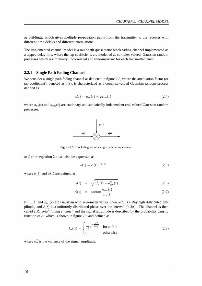
2.2.1 Single Path Fading Channel
We consider a single path fading channel as depicted in figure 2.5, where the attenuation factor (ortap coefficient), denoted as a(t), is characterized as a complex-valued Gaussian random processdefined as
a(t) = are(t) + jaim(t) (2.4)
where are(t) and aim(t) are stationary and statistically independent real-valued Gaussian randomprocesses.
����� � ����� �
��� �
Figure 2.5: Block diagram of a single path fading channel.
a(t) from equation 2.4 can also be expressed as
a(t) = α(t)ejφ(t) (2.5)
where α(t) and φ(t) are defined as
α(t) =√a2re(t) + a2
im(t) (2.6)
φ(t) = arctanaim(t)
are(t)(2.7)
If are(t) and aim(t) are Gaussian with zero-mean values, then α(t) is a Rayleigh distributed am-plitude, and φ(t) is a uniformly distributed phase over the interval [0; 2π). The channel is thencalled a Rayleigh fading channel, and the signal amplitude is described by the probability densityfunction of α, which is shown in figure 2.6 and defined as
fα(α) =
ασ2
αe− α2
2σ2α for α ≥ 0
0 otherwise(2.8)
where σ2α is the variance of the signal amplitude.
16

2.2. THE MULTIPATH FADING CHANNEL
� � �
�
Figure 2.6: Probability density function of α.
2.2.2 Multiple Paths Fading Channel
An example of a multipath Rayleigh fading channel model with corruption of AWGN is shown as atapped delay-line in figure 2.7. Each of the 4 paths are here characterized as a single path Rayleighfading channel as in figure 2.5, and each tap coefficient ai(t) for i = 1, 2, 3, 4 is described as inequation 2.5. D denotes a fixed time-delay of τ between the paths.
�����
����
��
�����
�
�
�
������� �������
�������
������� �������
������� � ������� !
�
Figure 2.7: Block diagram of multipath Rayleigh fading channel with corruption of AWGN. x(t) is the input signalat time t, and τ is a time-delay. The ai(t)’s are the tap coefficients involving both amplitude and phasecorruption, n(t) is the white Gaussian noise process, and r(t) is the output at time t.
The output of the channel depicted in figure 2.7 is expressed as
r(t) =4∑
i=1
x(t− (i− 1)τ)ai(t) + n(t) (2.9)
= x(t)a1(t) +
3∑
i=1
x(t− iτ)ai(t) + n(t) (2.10)
where the middle term on the right-hand side in equation 2.10 represents the ISI.
17

CHAPTER 2. CHANNEL MODEL
The achievable time resolution is 1/W , where W is the bandwidth of the transmitted signal. As-sume that the time-delays in figure 2.7 is 1/W . The number of multipath signal components iscalled the multipath spread and is denoted as Tm. In this example Tm = 1/W · 4 = 4/W . Thereciprocal of Tm is called the coherence bandwidth of the channel and is denoted as Bcb = 1/Tm.
If the signal bandwidth is greater than the coherence bandwidth, (W > Bcb), then the multipathcomponents are resolvable and the frequency components of the transmitted signal are affecteddifferently by the channel. In this case the received signal may be corrupted by ISI, and thechannel is called frequency selective. If, on the other hand, the signal bandwidth is less than thecoherence bandwidth, (W < Bcb), then the frequency components of the transmitted signal areaffected similarly, and in this case the channel is called frequency nonselective.
The considered multipath quasi-static block fading channel is frequency selective since W >Bcb = 1/Tm = W/4, thus ISI may be produced in the channel. A block diagram of the imple-mented 4-path quasi-static block fading channel is illustrated in figure 2.8. The input to the channelis the k’th burst sequence x(k), where the elements is x(k) are denoted as x(k)
i for i = 1, 2, . . . , 114.
a(k)1 , a(k)
2 , a(k)3 , and a(k)
4 are the tap coefficients for the k’th burst, and n(k)i is the white Gaussian
noise process realization. The output of the 4-path quasi-static block fading channel may be ex-pressed as
r(k)i = x
(k)i a
(k)1 + x
(k)i−1a
(k)2 + x
(k)i−2a
(k)3 + x
(k)i−3a
(k)4 + n
(k)i (2.11)
�����
���
�
�
�
��� �� �� ���
�
�� �� ��� �� � �� �
� ���� ���� ��� � ���
� ���� ���� ���� ���
� ���
� ���
Figure 2.8: Block diagram of the implemented 4-path quasi-static block fading channel.
2.3 The Matched Filter
We consider the channel model as a linear filter with the impulse response a(t) and corruptionby an additive white Gaussian noise process, n(t). The output of the channel, denoted as r(t),is the convolution of the impulse response of the channel with the transmitted signal, x(t), andcorruption by AWGN
r(t) = a(t) ∗ x(t) + n(t) =
∫ ∞
−∞a(τ)x(t− τ) dτ + n(t) (2.12)
18
2.3. THE MATCHED FILTER
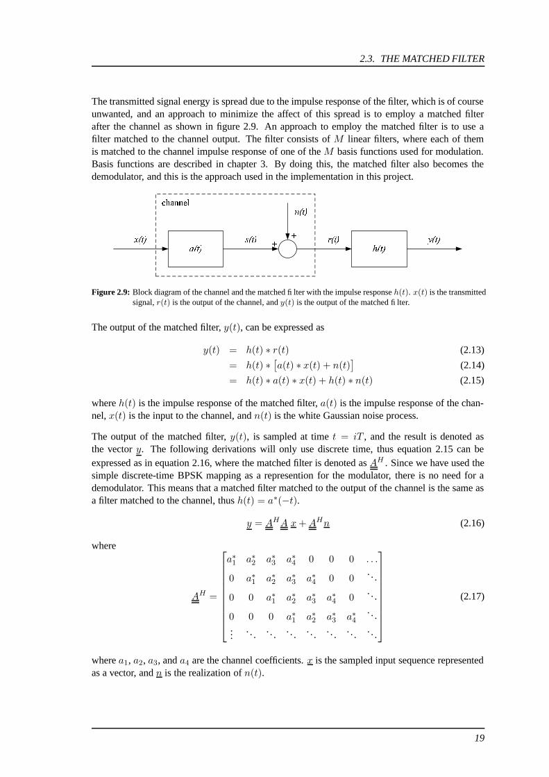
The transmitted signal energy is spread due to the impulse response of the filter, which is of courseunwanted, and an approach to minimize the affect of this spread is to employ a matched filterafter the channel as shown in figure 2.9. An approach to employ the matched filter is to use afilter matched to the channel output. The filter consists of M linear filters, where each of themis matched to the channel impulse response of one of the M basis functions used for modulation.Basis functions are described in chapter 3. By doing this, the matched filter also becomes thedemodulator, and this is the approach used in the implementation in this project.
����� � � ��� ����� �
��� ��� � � � � � � � ������ �
�������������
Figure 2.9: Block diagram of the channel and the matched filter with the impulse response h(t). x(t) is the transmittedsignal, r(t) is the output of the channel, and y(t) is the output of the matched filter.
The output of the matched filter, y(t), can be expressed as
y(t) = h(t) ∗ r(t) (2.13)
= h(t) ∗[a(t) ∗ x(t) + n(t)
](2.14)
= h(t) ∗ a(t) ∗ x(t) + h(t) ∗ n(t) (2.15)
where h(t) is the impulse response of the matched filter, a(t) is the impulse response of the chan-nel, x(t) is the input to the channel, and n(t) is the white Gaussian noise process.
The output of the matched filter, y(t), is sampled at time t = iT , and the result is denoted asthe vector y. The following derivations will only use discrete time, thus equation 2.15 can beexpressed as in equation 2.16, where the matched filter is denoted as AH . Since we have used thesimple discrete-time BPSK mapping as a represention for the modulator, there is no need for ademodulator. This means that a matched filter matched to the output of the channel is the same asa filter matched to the channel, thus h(t) = a∗(−t).
y = AHA x+AHn (2.16)
where
AH =
a∗1 a∗2 a∗3 a∗4 0 0 0 . . .
0 a∗1 a∗2 a∗3 a∗4 0 0. . .
0 0 a∗1 a∗2 a∗3 a∗4 0. . .
0 0 0 a∗1 a∗2 a∗3 a∗4. . .
.... . .
. . .. . .
. . .. . .
. . .. . .
(2.17)
where a1, a2, a3, and a4 are the channel coefficients. x is the sampled input sequence representedas a vector, and n is the realization of n(t).
19

CHAPTER 2. CHANNEL MODEL
The sampled output of the matched filter may also be expressed as
y = R x+AH n (2.18)
where R = AHA is the autocorrelation matrix of the channel.
2.3.1 Properties
Most wireless channels have time-varying characteristics, and the matched filters should thereforealso correspondingly change characteristics. In many communication systems, e.g. the GSM sy-stem, there is implemented a channel estimator which continuously estimates the characteristicsof the channel and updates the filter so it always matches the channel or the output of the channel.The channel estimator is not a part of this project and will therefore not be implemented. Perfectchannel knowledge is assumed to be known in the receiver at all time.
One important property of the matched filter is that it maximizes the Signal-to-Noise Ratio (SNR).To prove this property we consider the input to the matched filter, r(t), as defined in equation2.12. |a(t)| = 1 and therefore x(t) = s(t). At the sampling instant t = T , the sampled output-component of the matched filter is
y(T ) =
∫ T
0r(τ) · h(T − τ) dτ (2.19)
=
∫ T
0[s(τ) + n(τ)] · h(T − τ) dτ (2.20)
=
∫ T
0s(τ) · h(T − τ) dτ +
∫ T
0n(τ) · h(T − τ) dτ (2.21)
= ys(T ) + yn(T ) (2.22)
where h(t) is the matched filter, ys(T ) is the signal component, and yn(T ) is the noise component.
The SNR is defined as
SNR =
(S
N
)
0
=y2s(T )
E[y2n(T )]
(2.23)
The denominator is the noise variance and may be expressed as
E[y2n(T )] =
N0
2
∫ T
0h2(T − t) dt = σ2
n (2.24)
where σ2n denotes the noise variance.
20
2.3. THE MATCHED FILTER
To maximize the SNR, the numerator in equation 2.23 must be maximized while the denominatoris held constant. Applying the Cauchy-Schwarz inequality, the SNR can be expressed as
(S
N
)
0
=y2s(T )
E[y2n(T )]
(2.25)
=
[∫ T0 s(τ) · h(T − τ) dτ
]2
N02
∫ T0 h2(T − t) dt
(2.26)
≤∫ T0 s2(τ) dτ ·
∫ T0 h2(T − τ) dτ
N02
∫ T0 h2(T − t) dt
(2.27)
where the Cauchy-Schwarz inequality states that
[∫ ∞
−∞g1(t)g2(t) dt
]2
≤∫ ∞
−∞g21(t) dt
∫ ∞
−∞g22(t) dt (2.28)
and equality holds when g1(t) = Cg2(t) for any arbitrary constant C .
According to Cauchy-Schwarz’s inequality, the numerator in equation 2.26 is maximized whens(τ) = C · h(T − τ). If equality holds, the
∫ T0 h2(T − t) dt in both the numerator and the
denominator in equation 2.27 disappears, and the maximum SNR of the matched filter is
(S
N
)
0
=2
N0
∫ T
0s2(t) dt (2.29)
=2EsN0
(2.30)
where Es is the energy in each symbol after encoding.
21

CHAPTER
Modulation 3The purpose of a communication system is to deliver information to a user at the destination. Todo this, a message signal is created based on the information, and it is modified by a transmitterinto a signal suitable for transmission through the channel. The modification is achieved by meansof a modulation process, which varies some parameters of a carrier wave in accordance with themessage signal. The receiver re-creates a degraded version of the original message signal by usinga demodulation process, which is the reverse of the modulation process used in the transmitter.The reason for degration of the re-created message signal is due to the unavoidable presence ofnoise and distortion in the received signal, and this resulting degration is influenced by the type ofmodulation scheme used.
The modulation process can be classified into continuous-wave modulation and pulse modulation.For continuous-wave modulation, the carrier wave is a sinusoidal wave, and for pulse modulationthe carrier is a periodic sequence af rectangular pulses.
We consider discrete time BPSK modulation represented as a baseband signal. The input to themodulator is burst sequences in {0, 1}. The BPSK modulator (or mapper) maps each element inthe bursts sequences into a symbol in {−1,+1}.
To give a general understanding of how BPSK works, both the BPSK modulation for bandpasstransmission and the corresponding representation for baseband transmission are described in thischapter.
Consider a communication system, where the transmitted symbols belong to an alphabet of Msymbols denoted asm1,m2, . . . ,mM . In the case for BPSK, the alphabet consists of two symbols,thus the name Binary PSK. The transmitter codes for each duration T the symbol mi into a distinctsignal, si(t), suitable for transmission through the channel. si(t) is a real-valued signal waveform,and it occupies the full duration allotted to mi. The M signal waveforms, s1(t), s2(t), . . . , sM (t),can be represented as geometric representations, where they are linear combinations of K or-thonormal waveforms for K ≤ M . The procedure to construct the orthonormal waveforms iscalled the Gram-Schmidt orthogonalization procedure, and it is described in the first section ofthis chapter.
The references for this chapter are [Proakis et al., 2002] and [Haykin, 2001].
22

3.1. GRAM-SCHMIDT ORTHOGONALIZATION PROCEDURE
3.1 Gram-Schmidt Orthogonalization Procedure
Consider the set of M signal waveforms
S = {s1(t), s2(t), . . . , sM (t)} (3.1)
From the M signal waveforms in S we construct K ≤M orthonormal waveforms
Sψ = {ψ1(t), ψ2(t), . . . , ψK(t)} (3.2)
The k’th orthonormal waveform is defined as
ψk(t) =s′k(t)√Ek
(3.3)
where
s′k(t) = sk(t) −k−1∑
i=1
ck,i ψi(t) (3.4)
and Ek =
∫ ∞
−∞|s′k(t)|2 dt (3.5)
ψk(t) is a normalization of s′k(t) to unit energy. ck,i is a projection of sk(t) onto ψi(t), and s′k(t)is therefore orthogonal to ψi(t) (but not with unit energy).
The projection, ck,i, is defined as
ck,i = 〈sk(t), ψi(t)〉 =
∫ ∞
−∞sk(t)ψi(t) dt for i = 1, 2, . . . , k − 1 (3.6)
When the K orthonormal waveforms in Sψ are constructed, the M signal waveforms in S can beexpressed as linear combinations of the orthonormal waveforms
sm(t) =K∑
k=1
θm,kψk(t) for m = 1, 2, . . . ,M (3.7)
where
θm,k =
∫ ∞
−∞sm(t)ψk(t) dt (3.8)
The energy in each signal waveform, sm(t), is the sum of the energies in the K θ’s
Em =
∫ ∞
−∞|sm(t)|2 dt =
K∑
k=1
θ2m,k (3.9)
The signal waveforms may be expressed as a point in the K dimensional signal space, and the Kθ’s are the coordinates
sm = (θm,1, θm,2, . . . , θm,K) (3.10)
23

CHAPTER 3. MODULATION
It should be noted, that by applying the Gram-Schmidt orthogonalization procedure, you are guar-anteed to find a set of orhonormal waveforms for the signal waveforms, but in many cases it issimpler to construct the orthonormal functions just by inspection.
3.2 Binary Phase Shift Keying
Phase Shift Keying (PSK) is a continuous-wave modulation scheme for bandpass transmission,and it consists of M signal waveforms, s1(t), s2(t), . . . , sM (t). The signals in the M -ary PSKmodulation scheme can be represented by 2 orthonormal waveforms, ψ1(t) and ψ2(t), and byexpressing theM signal waveforms as points in a 2-dimensional signal space according to equation3.10, we have sm = (θm,1, θm,2). The PSK signal constellation for M = 2, 4, 8 is shown in figure3.1.
�
�
�����
�
�
�����
�
�
���
� �� � �� � �
� �
���
� �
� �
�
� �
���
���
���
���
Figure 3.1: PSK signal constellation for M = 2, 4, 8.
3.2.1 Bandpass Transmission
PSK consists of sine waveforms with the same frequency, and the information is conveyed by thephase. The signal waveforms for M -ary PSK are defined as
sm(t) = gT (t) cos(2πfct+ φm) for t ∈ [0, T ] (3.11)
where
gT (t) =
√2EsT
for t ∈ [0, T ] (3.12)
and φm = 2πm− 1
Mfor m = 1, 2, . . . ,M (3.13)
gT (t) is a rectangular pulse, Es is the transmitted signal energy per symbol, fc is the carrier fre-quency, T is the symbol duration time, and φm is the phase. fc is chosen so that fc = C
T for somefixed integer C , and T is positive.
24
3.2. BINARY PHASE SHIFT KEYING
The signal waveforms defined in equation 3.11 can be split up into two signals by viewing theangle of the cosine as a sum of two angles. Equation 3.11 can then be rewritten as
sm(t) =
√2EsT
[A1 cos(2πfct) −A2 sin(2πfct)
]for t ∈ [0, T ] (3.14)
where
A1 = cos(2πm− 1
M
)for m = 1, 2, . . . ,M (3.15)
and A2 = sin(2πm− 1
M
)for m = 1, 2, . . . ,M (3.16)
The 2-dimensional geometric point-representation stated in equation 3.10 can then be expressedas
sm = (θm,1, θm,2) =
(√Es cos
(2πm− 1
M
),√Es sin
(2πm− 1
M
))(3.17)
For BPSK, the modulation scheme has two signal waveforms s1(t) and s2(t), where φ1 = 0 andφ2 = π, or s2(t) = −s1(t), and the signal constellation for has only one orthonormal waveform
ψ1(t) =
√2
Tcos(2πfct) for t ∈ [0, T ]. (3.18)
The input to the modulator is a burst sequence, denoted as e, where the elements in e are denotedas ei ∈ {0, 1}. The transmitted signal after modulation, denoted as x(t), is expressed as
x(t) =
{s1(t) for ei = 0
s2(t) for ei = 1(3.19)
where s1(t) = +√ES · ψ1(t) and s2(t) = −√
ES · ψ1(t).
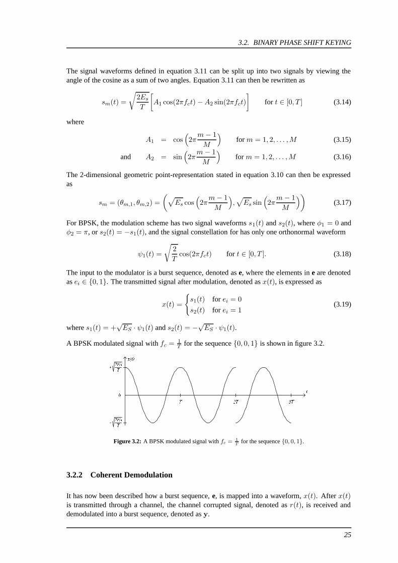
A BPSK modulated signal with fc = 1T for the sequence {0, 0, 1} is shown in figure 3.2.
������
� �� ��� �
��� �
������
Figure 3.2: A BPSK modulated signal with fc = 1T
for the sequence {0, 0, 1}.
3.2.2 Coherent Demodulation
It has now been described how a burst sequence, e, is mapped into a waveform, x(t). After x(t)is transmitted through a channel, the channel corrupted signal, denoted as r(t), is received anddemodulated into a burst sequence, denoted as y.
25

CHAPTER 3. MODULATION
���������� ��������� � dt
iT
TiT)(.
�−
��� ���������
)2cos()( 21 tft cT πψ =
� �"!$#&%$'�(*)$%,+ -/.10/)324 5�6�7 8 9$6:7 8 ;�6=<�>?8
@:A
Figure 3.3: A bandpass BPSK modulation scheme.
The system with BPSK modulation scheme is shown in figure 3.3. The channel corrupted receivedsignal, r(t), is multiplied with the orthonormal function for BPSK, ψ1(t), and the product is in-tegrated over the time duration T . The output of the integrator is sampled at each time instant iTand is also the output of the demodulator, y(iT ).
We assume that x(t) is transmitted through an AWGN channel, and the received signal, r(t), iscorrupted by AWGN. r(t) is the input to the demodulator, and the sampled output for the firstsymbol duration is computed as
y(T ) =
∫ T
0r(t)ψ1(t) dt (3.20)
=
∫ T
0[x(t) + n(t)]
√2
Tcos(2πfct) dt (3.21)
where n(t) is the contribution due to the corruption by the noise in the channel.
If we replace the contribution due to the channel corruption with nT =∫ T0 n(t)
√2T cos(2πfct) dt,
the expression in equation 3.21 can be rewritten as
y(T ) =
∫ T
0x(t)
√2
Tcos(2πfct) dt+ nT (3.22)
=
∫ T
0
√2EsT
cos(2πfct+ φm)
√2
Tcos(2πfct) dt+ nT (3.23)
=
∫ T
0
√2EsT
√2
T
[1
2cos(4πfct+ φm) +
1
2cos(φm)
]dt+ nT (3.24)
=1
2
√4EsT 2
∫ T
0
[cos(4πfct+ φm) + cos(φm)
]dt+ nT (3.25)
=
√EsT
[sin(4πfcT + φm) − sin(φm) + T cos(φm)
]+ nT (3.26)
26
3.2. BINARY PHASE SHIFT KEYING
Since fcT is a fixed integer, C , the expression in equation 3.26 can be reduced to
y(T ) =
√EsT
[sin(φm) − sin(φm) + T cos(φm)
]+ nT (3.27)
=√Es cos(φm) + nT (3.28)
and for BPSK, φm is either 0 or π, therefore
y(T ) =
{+√Es + nT for φm = 0
−√Es + nT for φm = π
(3.29)
3.2.3 Baseband Transmission
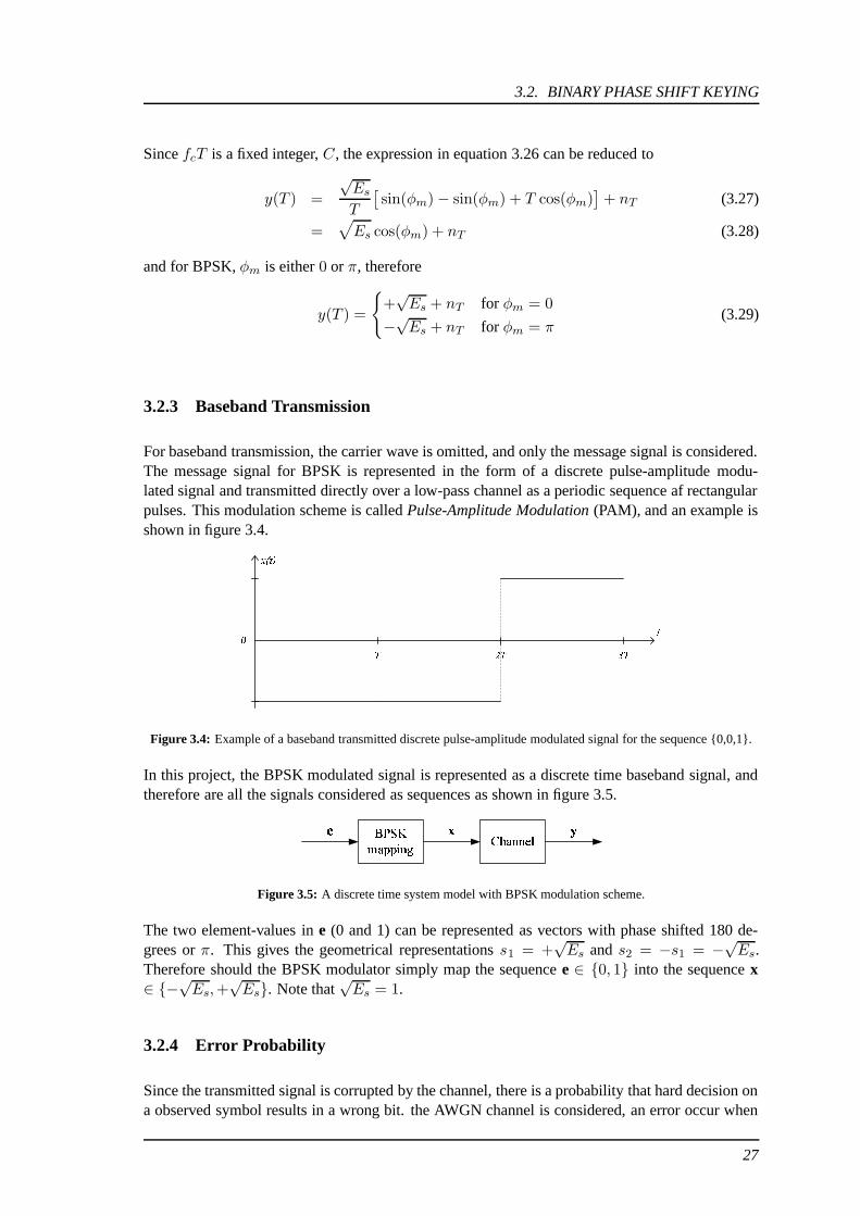
For baseband transmission, the carrier wave is omitted, and only the message signal is considered.The message signal for BPSK is represented in the form of a discrete pulse-amplitude modu-lated signal and transmitted directly over a low-pass channel as a periodic sequence af rectangularpulses. This modulation scheme is called Pulse-Amplitude Modulation (PAM), and an example isshown in figure 3.4.
� �� ��� ���
��� � �
Figure 3.4: Example of a baseband transmitted discrete pulse-amplitude modulated signal for the sequence {0,0,1}.
In this project, the BPSK modulated signal is represented as a discrete time baseband signal, andtherefore are all the signals considered as sequences as shown in figure 3.5.
� ���������������� ��� ���������
! "
Figure 3.5: A discrete time system model with BPSK modulation scheme.
The two element-values in e (0 and 1) can be represented as vectors with phase shifted 180 de-grees or π. This gives the geometrical representations s1 = +
√Es and s2 = −s1 = −√
Es.Therefore should the BPSK modulator simply map the sequence e ∈ {0, 1} into the sequence x∈ {−√
Es,+√Es}. Note that
√Es = 1.
3.2.4 Error Probability
Since the transmitted signal is corrupted by the channel, there is a probability that hard decision ona observed symbol results in a wrong bit. the AWGN channel is considered, an error occur when
27
CHAPTER 3. MODULATION
yi < 0 is observed when xi = +√Es is sent, or when yi > 0 is observed when xi = −√
Es is sent.
The conditional probability density function for yi given that xi = +√Es is defined as [Haykin, 2001]
fY |X(yi|xi = +√Es) =
1√πN0
e− 1
N0|yi−
√Es|2 (3.30)
The conditional symbol error-probability is then defined as
P (yi < 0|xi = +√Es) =
∫ 0
−∞fY |X(yi| +
√Es) dyi (3.31)
=1√πN0
∫ 0
−∞e− 1
N0|yi−
√Es|2 dyi (3.32)
=1√2π
∫ −√
2Es/N0
−∞e−
12z2 dz (3.33)
where
z =yi −
√Es√
N02
(3.34)
The conditional symbol error-probability in equation 3.33 can be rewritten as
Ps =1√2π
∫ −√
2Es/N0
−∞e−
12z2 dz (3.35)
=
∫ −√
2Es/N0
−∞q(z) dz (3.36)
= Q
(√2EsN0
)(3.37)
where
q(z) =1√2πe−
12z2 and Q(v) =
∫ ∞
vq(z) dz (3.38)
For BPSK the symbol error-probability is equal to the bit-error propability and therefore
Pb = Q
(√2EbN0
)= Q
(√2EsN0
)= Ps (3.39)
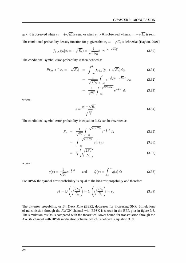
The bit-error propability, or Bit Error Rate (BER), decreases for increasing SNR. Simulationsof transmission through the AWGN channel with BPSK is shown in the BER plot in figure 3.6.The simulation results is compared with the theoretical lower bound for transmission through theAWGN channel with BPSK modulation scheme, which is defined is equation 3.39.
28

3.2. BINARY PHASE SHIFT KEYING
0 1 2 3 4 5 6 7 8 9 1010
−6
10−5
10−4
10−3
10−2
10−1
Eb/No [dB]
BE
R
Results of simulationsTheoretical bound
Figure 3.6: BER plot of the AWGN channel with BPSK.
29

CHAPTER
Convolutional Encoding 4The system model consider (23,33) convolutional coding as channel coding, since it is the schemespecified in the GSM standard. The input to the encoder is the info word, which is a sequence of224 info bits, and the output is the code word consisting of 456 code bits.
The purpose of channel coding is to provide reliable transmission of information in the presenceof noise by adding redundancy to the transmitted signal in a controlled manner. In general, thechannel encoder separates or segments an incoming bit stream into equal length blocks of k binarydigits and maps each k-bit block, which is called the info word, into an l-bit code word block,where l > k. The set of code words contains 2k code words of length l code bits. After transmis-sion and detection in the receiver, the channel decoder finds the most likely code word from thereceived l-bit word, and inversely maps it into the corresponding k-bit info word.
In this project, convolutional block codes have been studied. Block codes process the info bits ona block-by-block basis, so as to treat each block of info bits independently from each other. Theblock codes map k-bit info words into l-bit code words, which imply that l− k additional bits areadded to the k-bit info word to form the l coded bits.
This chapter will describe the convolutional encoder with emphasis on the (23,33) convolu-tional encoder, which is specified in the GSM standard. The primary reference of this chapteris [Proakis et al., 2002].
4.1 The Convolutional Encoder
For convolutional codes the encoded code bits depend not only on the current k info bits but alsoon the previous m info bits.
Rate 1/2 convolutional codes have a simple encoding scheme. The k info bits are passed sequen-tially to m linear shift registers, which are basically delay elements, and these k info bits aremapped into l code bits. These code bits are formed from modulo-2 additions of the contents ofthe memory (m-shift registers) and the info bits. After the k info bits are passed, m zeros are alsopassed through the encoder so as to reset the encoder to all-zero state and make it ready for nexttransmission. The code rate of binary convolutional encoder is Rc = k/l.
30

4.1. THE CONVOLUTIONAL ENCODER
Convolutional codes are specified by there generators denoted as g1 and g2, and the specific code iscalled a (g1,g2) convolutional code. The generators have an octal value which define the mappingprocess from the k info bits to the l code bits. An example of a convolutional encoder havinggenerators (5, 7) with code rate Rc = 1/2 is shown in figure 4.1. The input is the info wordsequence denoted as d, where the elements in d is denoted as di for i = 1, 2, . . . , k. The output isthe code word sequence, denoted as c, where the elements in c is denoted as ci for i = 1, 2, . . . , k,
and ci consist of two elements, c(1)i and c(2)i , so the code word sequence contains l = 2k elements.
D D���
� �
� ����� � � � ��
� �
� �
�
� �� �
���
� � �
Figure 4.1: (5,7) convolutional encoder. di is the uncoded 1-dimensional info word element, and ci is the 2-dimensionalcode word element. D denotes a time-delay. The binary values for the generators, g1 = 5 and g2 = 7, is101 and 111 respectively.
Example 4.1 will show the mapping from the info word sequence d into the code word sequence cwith the (5,7) generators and code rate Rc = 1/2.
EXAMPLE 4.1: The sequence d = {1, 0, 1, 0, 0} is encoded with a 12 rate (5,7) convolutional
encoder. It is assumed that the encoder is in all zero state before encoding. ⊕ denotesmodulo-2 addition.
The elements in c(1) and c(2) are calculated as
c(1) = {d1 ⊕ 0 , d2 ⊕ 0 , d3 ⊕ d1 , d4 ⊕ d2 , d5 ⊕ d3} (4.1)
= {1, 0, 0, 0, 1} (4.2)
c(2) = {d1 ⊕ 0 ⊕ 0 , d2 ⊕ d1 ⊕ 0 , d3 ⊕ d2 ⊕ d1 , (4.3)
d4 ⊕ d3 ⊕ d2 , d5 ⊕ d4 ⊕ d3}= {1, 1, 0, 1, 1} (4.4)
The elements in c is then calculated as
c = {c(1)1 c(2)1 , c
(1)2 c
(2)2 , c
(1)3 c
(2)3 , c
(1)4 c
(2)4 , c
(1)5 c
(2)5 } (4.5)
= {11, 01, 00, 01, 11} (4.6)
where c(1)i and c(2)i are the elements in ci for i = 1, 2, ..., 5.
The GSM encoder has the generators g1 = 23 and g2 = 33 and code rate Rc = 1/2 as illustratedin figure 4.2. The code word is computed the same way as depicted in example 4.1, except thatc(1)i and c(2)i is now calculated as
c(1)i = di ⊕ di−3 ⊕ di−4 (4.7)
c(2)i = di ⊕ di−1 ⊕ di−3 ⊕ di−4 (4.8)
31

CHAPTER 4. CONVOLUTIONAL ENCODING
� ����
� �
� ����� � � � �
� �
� �
� �
� � �� �
���
� � �
��
��
��
Figure 4.2: (23,33) convolutional encoder. The binary values for g1 = 23 and g2 = 33 is 10011 and 11011 respectively,as depicted in the figure.
In the implemented system, an info word, d, consisting of 224 info bits is to be encoded usingthe (23,33) encoding scheme. Before encoding, 4 zeros are added to d to ensure zero-state. Theresulting code word, c, has the size of (224 + 4) · 2 = 456 symbols.
The elements in c are computed as
ck =
{dko
⊕ dko−3 ⊕ dko−4 for k is odd
dke⊕ dke−1 ⊕ dke−3 ⊕ dke−4 for k is even
(4.9)
for k = 1, 2, . . . , 456. ko = k+12 and ke = k
2 .
4.2 Properties of Convolutional Codes
Convolutional codes can be regarded as a finite state machine, represented by a state diagram. Eachof the 2m states in the state diagram, where m is the number of memory elements, is representedby a circle and transitions among the states are represented by lines connecting these circles. Onevery line, input and output caused by that transition are represented. A state diagram for theconvolutional encoder having generators (5,7) is shown in figure 4.3. Dashed line denotes ’0’-input and solid line denotes ’1’-input.
Convolutional codes may also be described by a trellis diagram. The state diagram fails to repre-sent the transitions as time evolves. The trellis diagram is able to represent the transitions amongthe various states as the time evolves. This is shown by repeating the states vertically along thetime axis (horizontal discrete axis). See figure 4.4. Every repetition of the states is called a stage,and the step from one state to the next is called a transition (or branch). The transition from onestate to another in the next stage is represented by a dashed line for ’0’-input and solid line for’1’-input. In other words, it can be said that the trellis diagram is a repetition of the state diagramalong the time axis.
The trellis diagram contains several paths, each path corresponding to a distinct code word. Anexample of a trellis diagram for (5,7) convolutional codes is shown in figure 4.4. It is assumed thatthe encoder is in all zero state before encoding, thus has the first stage only transitions from state’00’. The two digits connected to each transition is the output of the encoder corresponding to thetransition.
32

4.2. PROPERTIES OF CONVOLUTIONAL CODES
10 01
00
11
���
���
���
���
���
���
���
���
Figure 4.3: State diagram of a (5,7) convolutional encoder. Dashed line denotes ’0’-input and solid line denotes ’1’-input.
00
01
10
11
00 00 00 00 00
11 11 11 11 11
01 01 01 01
10 10 10 10
10 10 10
01 01 01
00 00 00
11 11 11
stat
es
time
Figure 4.4: Trellis diagram of a (5,7) convolutional encoder. Dashed line denotes ’0’-input and solid line denotes’1’-input.
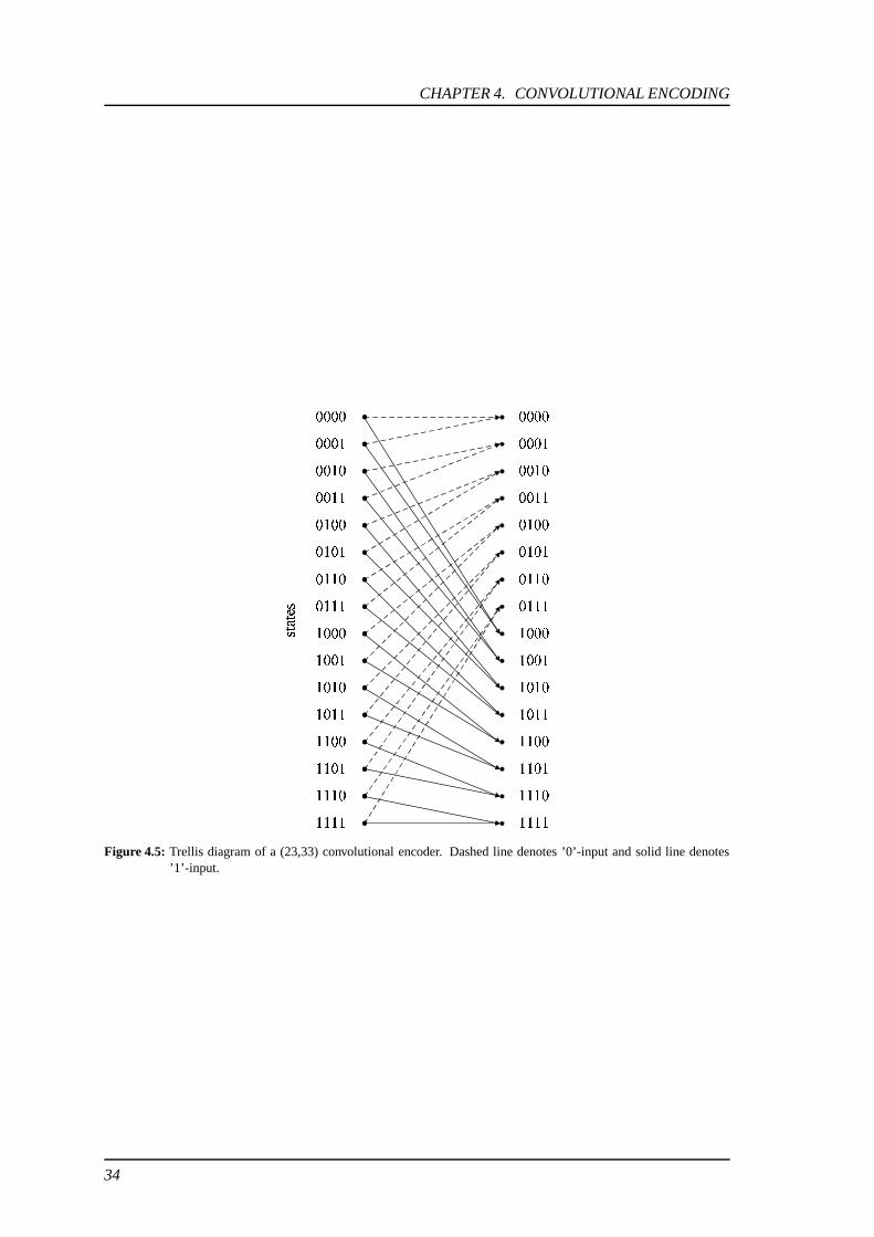
The trellis diagram for (23,33) convolutional codes has 2m = 24 = 16 states as depicted in figure4.5. The figure shows only one transition.
33
CHAPTER 4. CONVOLUTIONAL ENCODING
�������
�� �� ��
������
������
������
��� ���
��� ��
�������
�������
�������
������
������
������
��� ���
��� ��
�������
�������
�������
������
���� �
������
�������
������
����� �
�������
�������
������
���� �
������
�������
������
����� �
�������
Figure 4.5: Trellis diagram of a (23,33) convolutional encoder. Dashed line denotes ’0’-input and solid line denotes’1’-input.
34

CHAPTER
Convolutional Decoding usingthe Viterbi Algorithm 5The decoder maps the observed code word of 456 code bits into an estimated info word of 224info bits. The GSM standard does not specify any decoding algorithm, but an often used channeldecoder for convolutional coding is a Maximum Likelihood (ML) decoder called the Viterbi De-coder. The basic idea of ML-decoding is to compare the received sequence with all the possiblecode word sequences and then calculate the corresponding likelihoods. The sequence with thehighest likelihood is selected as the estimated code word, which is then mapped into the estimatedinfo word.
The Viterbi Algorithm and the performance of the Viterbi Decoder is described in this chapter.The reference for the chapter is [Proakis et al., 2002], unless any other is stated.
5.1 Maximum Conditional Probability
The Viterbi Decoder finds the closest code word to the observed sequence by processing the se-quences on a bit-by-bit basis. This means that the Viterbi Algorithm selects the code word thatmaximizes the conditional probability. [Morelos-Zaragoza, 2002]
The conditional probability for a code word c, given the observed sequence y is
P (c|y) =
l∏
j=l
P (cj |y2j−1, y2j) (5.1)
where yj is the j’th element in y. cj is the j’th element in c, and l is the length of the code word.
35

CHAPTER 5. CONVOLUTIONAL DECODING USING THE VITERBI ALGORITHM
The estimated code word c can then be expressed as
c = arg maxc∈C
P (c|y) = arg maxc∈C
l∏
j=l
P (cj |yj) (5.2)
where C is the set of code words.
For the AWGN channel it is equivalent to choosing the code word that minimizes the squaredEuclidean distance
c = arg minc∈C
dE(c,y) = arg minc∈C
l∑
j=1
‖cj − yj‖2 (5.3)
When using the squared Euclidean distance, it is called soft-decision decoding. Another way tomake decisions is to use the hamming distance, and this is called hard-decision decoding.
The hamming distance is defined as
dH(c,y′) =l∑
j=1
cj ⊕ y′j (5.4)
where y is turned into a binary sequence, y, by making hard-decisions on the individual elementsin y.
The output of the Viterbi decoder is an estimated info word d, corresponding to the estimated codeword c.
5.2 Optimal Path Through the Trellis
Convolutional codes can be represented by a trellis diagram as described in chapter 4. The ViterbiDecoder searches for the path through the trellis that is at minimum distance from received se-quence. This indicates the most likely transmitted code word, and thereby the most likely infoword corresponding to that code word.
To describe how the Viterbi Decoder works, we will follow example 5.1, where hard-decisionsdecoding is used on a (5,7) convolutional encoded sequence with code rate Rc = 1/2.
EXAMPLE 5.1: The sequence y′ = {11, 11, 01, 01, 10} is hard-decisions of the observed se-quence y, and the transmitted code word is encoded with a 1
2 rate (5,7) convolutional encoderas in example 4.1 on page 31. y′ has three errors compared to the code word in example 4.1,where c = {11, 01, 00, 01, 11}. It is assumed that the encoder was in all zero state beforeencoding.
Each node in the trellis has a state-value, denoted as S (k)i , corresponding to the path with
the shortest hamming distance to that node. The transition to this node with the shortestHamming distance is called the "survivor", and the other is discarded. The state-values aregathered in a state matrix, denoted as M(S
(k)i ), as shown in table 5.1.
36

5.2. OPTIMAL PATH THROUGH THE TRELLIS
k\i 0 1 2 3 4 5
1 (’00’) S(1)0 S
(1)1 S
(1)2 S
(1)3 S
(1)4 S
(1)5
2 (’01’) S(2)0 S
(2)1 S
(2)2 S
(2)3 S
(2)4 S
(2)5
3 (’10’) S(3)0 S
(3)1 S
(3)2 S
(3)3 S
(3)4 S
(3)5
4 (’11’) S(4)0 S
(4)1 S
(4)2 S
(4)3 S
(4)4 S
(4)5
Table 5.1: State matrix, M(S(k)i ), where k denotes the state and i denotes the stage. S
(k)0 is the initial state-values for
stage k.
The state-values are calculated by the following algorithm
S(k)i = S
(j)i−1 + dH(y′i, ci) for i = 1, 2, . . . , 5 and k = 1, 2, 3, 4 (5.5)
where S(j)i−1 is the previous state-value in the survivor path. Since the encoder was in all zero
state before encoding, the initial state-values are
S(k)0 = 0 for k = 1 (5.6)
S(k)0 = ∞ for k = 2, 3, 4 (5.7)
All the necessary state-values are calculated and placed in the trellis diagram in figure 5.1.The trellis ends in ’00’-state, because two zeros have been added in the end of the sequencein the encoder in order to get the encoder in all zero state after encoding. The crosses denotediscarded transitions. As shown in the figure, the final survivor-path, denoted as a blue path,indicates that the most likely code word was {11, 01, 00, 01, 11}, which corresponds to theinfo word {1, 0, 1, 0, 0}, which also was the case.
�
�
� � �
�
�
�
�
�
�
�
� ���� ���
��
���
���
��
��
����
�����
��
������ ��� ���
��� ���
��� ���� �
���
���
���
�� �� �����
��� ��� �� ����� ��� � �! "# # # #
Figure 5.1: The trellis diagram used as hard-decision Viterbi decoding. The dashed lines correspond to ’0’-input andthe solid lines to ’1’-input. The numbers above the state-points is the state-values, and the blue path is thefinal survivor-path, and it corresponds to the info word {1, 0, 1, 0, 0}.
37
CHAPTER 5. CONVOLUTIONAL DECODING USING THE VITERBI ALGORITHM
The decoding technique for the (23,33) convolutional decoder is the same as for (5,7), except thatthe trellis diagram has 16 states in stead of 4, which is explained in chapter 4 and depicted in figure4.5.
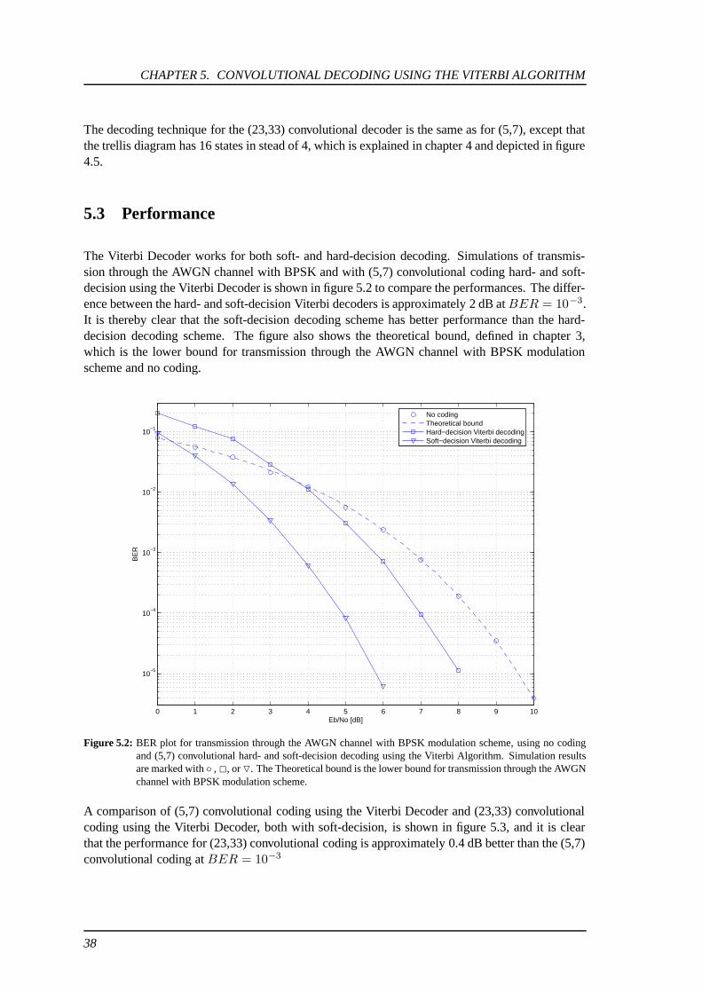
5.3 Performance
The Viterbi Decoder works for both soft- and hard-decision decoding. Simulations of transmis-sion through the AWGN channel with BPSK and with (5,7) convolutional coding hard- and soft-decision using the Viterbi Decoder is shown in figure 5.2 to compare the performances. The differ-ence between the hard- and soft-decision Viterbi decoders is approximately 2 dB atBER = 10−3.It is thereby clear that the soft-decision decoding scheme has better performance than the hard-decision decoding scheme. The figure also shows the theoretical bound, defined in chapter 3,which is the lower bound for transmission through the AWGN channel with BPSK modulationscheme and no coding.
0 1 2 3 4 5 6 7 8 9 10
10−5
10−4
10−3
10−2
10−1
Eb/No [dB]
BE
R
No codingTheoretical boundHard−decision Viterbi decodingSoft−decision Viterbi decoding
Figure 5.2: BER plot for transmission through the AWGN channel with BPSK modulation scheme, using no codingand (5,7) convolutional hard- and soft-decision decoding using the Viterbi Algorithm. Simulation resultsare marked with ◦ , 2, or O. The Theoretical bound is the lower bound for transmission through the AWGNchannel with BPSK modulation scheme.
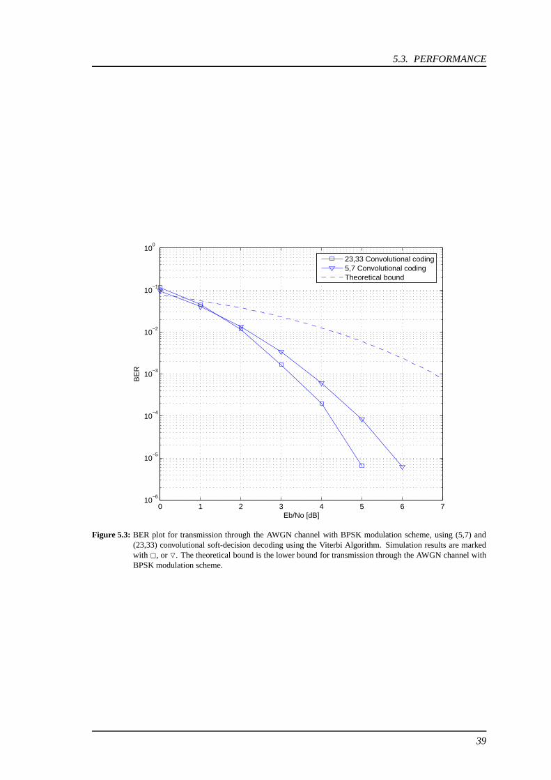
A comparison of (5,7) convolutional coding using the Viterbi Decoder and (23,33) convolutionalcoding using the Viterbi Decoder, both with soft-decision, is shown in figure 5.3, and it is clearthat the performance for (23,33) convolutional coding is approximately 0.4 dB better than the (5,7)convolutional coding at BER = 10−3
38
5.3. PERFORMANCE
0 1 2 3 4 5 6 710
−6
10−5
10−4
10−3
10−2
10−1
100
Eb/No [dB]
BE
R
23,33 Convolutional coding5,7 Convolutional codingTheoretical bound
Figure 5.3: BER plot for transmission through the AWGN channel with BPSK modulation scheme, using (5,7) and(23,33) convolutional soft-decision decoding using the Viterbi Algorithm. Simulation results are markedwith 2, or O. The theoretical bound is the lower bound for transmission through the AWGN channel withBPSK modulation scheme.
39

CHAPTER
Equalization 6InterSymbol Interference (ISI) is produced in the channel due to multipath propagation. A tech-nique to eliminate (or reduce) the effect of ISI is to apply an equalizer after the matched filter.The equalizer should adapt to the channel characteristics, which are often evaluated runningly inreal time applications such as e.g. the GSM system. In this project, we assume to have perfectknowledge of the channel characteristics at all time.
This chapter will describe two different equalizers, namely the Viterbi Equalizer and the Max-log-MAP Equalizer.
The input signal to the equalizer in the system model considered in this project is modelled by thechannel encoder, the interleaver, the modulator, and the channel. The model for the input signal isdescribed in the first section of this chapter.
The references used for this chapter are [Proakis et al., 2002] and [Morelos-Zaragoza, 2002], un-less others are stated.
6.1 Signal Model
The input to the equalizer is called the signal model and is a result of the encoding process, theinterleaving process, the modulation process, and transmission through the channel. A block dia-gram of these processes is shown in figure 6.1.
� ����� ���������� ��� ������ ���
����� � � ����� � �!���!"#� $"%� ��� � �'&�� ��)( *%����� ��+
��������� � �-,. ��� ��� � �/* � � � ���
0 1�2 � 3�45 ��� ��� � � �6 ��� 798�:�;. ������ ��� �
< 1�2 � 3�4 = 1)2 � 3!4 > 1 $)3?�#3�4 @BAC@
5 ��*#EDF � �����GH&I� � "J �� � DE � �G-K!LH&�� � "
GM&-� � "N� "3�3)GH&�� � "G . ������ �)� � �M&�� � "#� "3!3?GO" P . &��� "
GF�&Q" ��� � � " � �!� � ��� � "3�3)G "N�*#� $ " P . &��� "
Figure 6.1: Block diagram of the signal model.
40
6.1. SIGNAL MODEL
The input to the (23,33) convolutional encoder is a sequence, denoted as d, of 224 bits in {0, 1}.This sequence is called the info word, and the elements, denoted as di, are generated randomly.
The output sequence of the encoder is the input sequence to the interleaver and is called the codeword. The code word is denoted as c and consists of 456 bits in {0, 1}. 4 tail bits are added to the224 bits in the info word, and the new sequence of 228 bits are mapped into the code word as
ci = {c(1)i c(2)i } = {c2i−1 c2i} for i = 1, 2, . . . , 228 (6.1)
where
c(1)i = di ⊕ di−3 ⊕ di−4 (6.2)
c(2)i = di ⊕ di−1 ⊕ di−3 ⊕ di−4 (6.3)
⊕ denotes modulo-2 addition.
Equation 6.1 can also be expressed as
ck =
{dl ⊕ dl−3 ⊕ dl−4 for k is odd
dm ⊕ dm−1 ⊕ dm−3 ⊕ dm−4 for k is even(6.4)
for k = 1, 2, . . . , 456. l = k+12 and m = k
2 .
The code word of 456 bits is the input to the interleaver. The code word is interleaved over 4 blocks(or sequences) and transmitted sequentially in 4 bursts. The interleaver sequence, consisting of 4bursts, is denoted as I = {e1 e2 e3 e4}, and each element in eB , denoted as eB,j is computed as
eB,j = ck for k = 1, 2, . . . , 456 (6.5)
where
B = [(k − 1) mod 4] + 1 (6.6)
j = 2[49(k − 1) mod 57] + [(k − 1) mod 8] div 4 (6.7)
B ∈ {1, 2, 3, 4} is the burst number, and j ∈ {1, 2, . . . , 114} is the bit number in burst B.
The input to the modulator is the interleaver sequence, and each element in the sequence is mappedas
xk =
{−1 for Ik = 0
+1 for Ik = 1(6.8)
where xk is an element in the transmitted sequence, denoted as x, and Ik is an element in I.
In chapter 2 we expressed the sampled output of matched filter as a vector
y = R x+AHn (6.9)
where AH is the impulse response of the matched filter, R = AHA is the autocorrelation matrixof the channel, and n is the realization of a white Gaussian noise process.
41
CHAPTER 6. EQUALIZATION
AH is defined as
AH =
a∗1 a∗2 a∗3 a∗4 0 0 0 . . .
0 a∗1 a∗2 a∗3 a∗4 0 0. . .
0 0 a∗1 a∗2 a∗3 a∗4 0. . .
0 0 0 a∗1 a∗2 a∗3 a∗4. . .
.... . . . . . . . . . . . . . . . . . . . .
(6.10)
where a1, a2, a3, and a4 are the coefficients in the channel, x is the sampled input sequence to thechannel represented as a vector, and n is the realization of n(t). al = zn + jzn for l = 1, 2, 3, 4,where zn is a realization of a normalized random process with variance 1 and zero-mean. j denoteshere the imaginary part.
We consider the output of the matched filter as a sequence of 456 bits, corresponding to one codeword, and we denote it as y. Each element in y is computed as
yk =(R x
)k
+(AHn
)k
(6.11)
The last term in equation 6.11 may be expressed as(AHn
)k
= a1nk + a2nk−1 + a3nk−2 + a4nk−3 (6.12)
where
nk =
√1Eb
N0
· zn (6.13)
zn is a realization of a normalized random process with variance 1 and zero-mean. For furtherdetails about generating nk we refer to appendix A.4.1 on page 71 concerning generation the ad-ditive white Gaussian noise.
The first term in equation 6.11 may be expressed as(R x
)k
= %41xk+3 + %31xk+2 + %21xk+1 + %11xk + %12xk−1 + %13xk−2 + %14xk−3 (6.14)
where
%11 = a21 + a2
2 + a23 + a2
4 (6.15)
%21 = %12 = a1a2 + a2a3 + a3a4 (6.16)
%31 = %13 = a1a3 + a2a4 (6.17)
%41 = %14 = a1a4 (6.18)
42

6.2. MAXIMUM-LIKELIHOOD SEQUENCE DETECTION
6.2 Maximum-Likelihood Sequence Detection
The equalizer finds the most likely sequence of transmitted symbols based on the observed symbolsand knowledge of the channel. A model of the channel, the matched filter, and the equalizer isshown in figure 6.2, where x is the transmitted code word, A is the channel, n is a realization of awhite Gaussian noise process, AH is the matched filter, y is the observed code word, specified inequation 6.9, and x is the estimated code word.
Ax
n
++ A �
ye q u a l i z e r
x�
Figure 6.2: A model of the channel, matched filter and equalizer
The estimated sequence of code bits, denoted as x, is the sequence with the highest probability ofthe observed sequence, y
x = arg maxx∈X
P (y | x) (6.19)
= arg maxx∈X
{ 1√2πσn
e− (y−x)2
2σ2n
}(6.20)
= arg maxx∈X
{log
1√2πσn
(−
(y − x)2
2σ2n
)}(6.21)
= arg maxx∈X
{−(y − x)2
}(6.22)
where X is the set of possible code words, and σ2n is the noise variance.
The channel corrupts the transmitted signal by white Gaussian noise, but after the matched filterthe noise is no longer white, which makes it more difficult to remove. To compensate for this,and make equation 6.22 usable, a whitening filter is applied to the observed signal described inequation 6.9
(AH)−1 y = (AH)−1 R x+ (AH)−1 AH n (6.23)
z = A x+ n (6.24)
where z = (AH)−1y is the output of the whitening filter.
The most likely sequence is when n is minimized, thus equation 6.22 can be written as equation6.25, using the least square estimate.
x = arg minx∈X
{‖z −A x‖2
}(6.25)
43

CHAPTER 6. EQUALIZATION
Equation 6.25 can be rewritten as
x = arg minx∈X
{(z −A x)H(z −A x)
}(6.26)
= arg minx∈X
{zH z + xH AH A x− 2Re{xH AH z}
}(6.27)
As we want to minimize with respect to x, zHz can be omitted. Note that AHz = y.
x = arg minx∈X
{xH R x− 2Re{xH AH z}
}(6.28)
= arg minx∈X
{Σi
Σj%ij x
∗i xj − 2Re{Σ
ix∗i yi}
}(6.29)
= arg minx∈X
{Σi|xi|2 + 2Re{Σ
i
i−1Σj=0
%ij x∗i xj} − 2Re{Σ
ix∗i yi}
}(6.30)
where %ij is the element in R on row i, column j, and xi is the i’th element in x. The transitionfrom equation 6.29 to equation 6.30 is due to the fact that %i,j = %∗j,i, which can easily be shown
using equation 2.17 on page 19 and R = AHA.
Since xi = ±1 ⇒ |xi|2 = 1,∑
i |xi|2 can be omitted.
x = arg minx∈X
{2Re{Σ
i
i−1Σj=0
%ij x∗i xj} − 2Re{Σ
ix∗i yi}
}(6.31)
= arg minx∈X
{Re{Σ
i(i−1Σj=0
(%ij x∗i xj) − x∗i yi}
}(6.32)
= arg minx∈X
{Re{Σ
ix∗i (
i−1Σj=0
(%ij xj) − yi)}}
(6.33)
This means that we need to minimize the expression in equation 6.33, in the following called themetric. The branch metric, shown i equation 6.34, can be calculated for each possible branch.
Re{x∗i (i−1Σj=0
(%ij xj) − yi)} (6.34)
Notice that the whitening filter was just used for derivation and is not needed in the implementationof the equalizer.
6.3 Viterbi Equalizer
Maximum likelihood sequence detection is an optimum detection, and is often used when having asmall number of states and/or short sequences. The basic idea is to compare the received sequencewith all the possible sequences and then calculate the corresponding likelihoods. The sequencewith the highest likelihood is then selected as the estimate of the transmitted sequence.
44

6.4. MAX-LOG-MAP EQUALIZER
0-1,-1
-1,1
1,-1
1,1
states
, k
Figure 6.3: A trellis diagram used in the Viterbi Algorithm. The blue path is the most likely path. The crosses showwhich paths has been omitted.
The channel can be expressed by a trellis diagram, as shown in figure 6.3, where each path throughthe diagram corresponds to a different sequence.
The Viterbi Algorithm, described in chapter 5 on page 35, is a maximum likelihood detectionmethod using the fact that only the most likely path to a given state at a given stage can be a partof the most likely path to another stage, thus all other paths to this first state can be discarded.As stated in equation 6.33 the sum of the metric of each transition in the trellis must be minimizedTo find the most likely sequence it is necessary to go through the trellis diagram from left to right,and for each node find the most likely sequence (called the survivor) and discard the other. If eachnode has a value ξ which is the weight of the most likely path, this ξ can be calculated as
ξi,k = maxj
[ξi,j + ζi,j,k] (6.35)
where ξi,k is the value of the node at stage i, state k, and ζi,j,k is the branch metric between statej and k at stage i.
A number of zeros, corresponding to the number of paths in the channel, has to be added to eachsequence before modulation. This is to make sure the finishing state is known. It is then possibleto backtrack from this state, through the survivors, thus finding the most likely path.
When the most likely sequence has been found, it is used as the output of the equalizer. Thisoutput is called hard output, as it only contains a sequence of 1’s and 0’s, and thus discards someinformation.
6.4 Max-log-MAP Equalizer
The Viterbi Equalizer described in the previous section defines the most likely sequence of sym-bols.
The output of the equalizer is often further processed. For instance a decoder is applied if theinfo word in encoded. To increase the amount of information passed to the decoder, and therebypossibly increasing the performance, an extended algorithm is needed. This algorithm must result
45

CHAPTER 6. EQUALIZATION
in not only the estimated sequence, but also an estimate of the reliability of each symbol in thesequence. The Max-log-MAP algorithm, described in this section, has this property, and it resultsin a soft value representation for each symbol, namely the logarithm of the Maximum A posterioriProbability (MAP).
In this section the MAP algorithm is described first, and then the modification, Max-log-MAP, isshown.
6.4.1 MAPWe define the probabilities α, β and γ in the following way [Bahl et al., 1974]
α(k)i , P (xi = uk ; y1, y2, ..., yi) (6.36)
β(k)i , P (yi+1, yi+2, ..., yL | xi = uk) (6.37)
γ(j,k)i , P (xi = uk ; yi | xi−1 = uj) (6.38)
where x= [x1, x2, ..., xL] is the transmitted sequence of symbols, y= [y1, y2, ..., yL] is the receivedsequence, uk ∈ {−1,+1} is the value of xi corresponding to state k, and L is the length of thesequence.
The MAP algorithm also uses the trellis diagram. Each node in the trellis has an α and a β attached,and each transition has a γ attached. Since there is several transitions to each node, equations 6.36and 6.37 can be rewritten as
α(k)i =
∑
j
P (xi−1 = uj , y1, y2, ..., yi−1) · P (xi = uk , yi | xi−1 = uj) (6.39)
=∑
j
α(j)i−1 · γ
(j,k)i (6.40)
β(k)i =
∑
j
P (yi+2, yi+3, ..., yL | xi+1 = uj) · P (xi+1 = uj , yi+1 | xi = uk) (6.41)
=∑
j
β(j)i+1 · γ
(k,j)i+1 (6.42)
for j = 1, 2, . . . ,M , where M is the number of states.
The a posteriori probability of state k at stage i is defined as
P (xi = uk|y) =∑
j
P (xi−1 = uj , xi = uk , y1, y2, ..., yL) (6.43)
=∑
j
P (xi−1 = uj , y1, y2, ..., yL) · P (yi+1, ..., yL | xi = uk) (6.44)
· P (xi = uk , yi | xi−1 = uj)
=∑
j
α(j)i−1 · β
(k)i · γ(j,k)
i (6.45)
46

6.4. MAX-LOG-MAP EQUALIZER
6.4.2 Log-MAP
Multiplication is rather computational expensive, thus an approach to decrease the complexity, thelog-MAP Algorithm is introduced. The log-probabilities α′, β′ and γ′ are then computed as
α′(k)i = log α
(k)i = log
(∑
j
α(j)i−1 · γ
(j,k)i
)(6.46)
β′(k)i = log β
(k)i = log
(∑
j
β(j)i+1 · γ
(k,j)i+1
)(6.47)
γ′(j,k)i = log γ
(j,k)i (6.48)
The branch metric defined in equation 6.34 can also be used for log-MAP since it is based on thelogarithm of the probabilities.
γ′(j,k)i = Re{x∗i (
i−1Σj=0
(%ij xj) − yi)} (6.49)
where % is the elements of R, xi is an element in x, and yi is an element in y.
6.4.3 Max-log-MAP
The α′’s and β′’s in equations 6.46 and 6.47 are still computational expensive, so the assumptionin equation 6.51 is used to reduce complexity, resulting in equation 6.54 and 6.57.
log(δ1 + δ2) = max[log(δ1), log(δ2)
]+ log
(1 + e−| log δ1+log δ2|) (6.50)
≈ max[log(δ1), log(δ2)
](6.51)
α′(k)i ≈ max
j
[log(α
(j)i−1 · γ
(j,k)i
)](6.52)
= maxj
[log(α
(j)i−1
)+ log
(γ
(j,k)i
)](6.53)
= maxj
[α′(j)i−1 + γ
′(j,k)i
](6.54)
β′(k)i ≈ max
j
[log(β
(j)i+1 · γ
(k,j)i+1
)](6.55)
= maxj
[log(β
(j)i+1
)+ log
(γ
(k,j)i+1
)](6.56)
= maxj
[β′(j)i+1 + γ
′(k,j)i+1
](6.57)
This can be represented in a trellis diagram like for the Viterbi Algorithm, but the difference is thateach node in the trellis diagram has now two values, α′(k)
i and β′(k)i respectively, and the branches
have the values γ ′(k,j)i . Such a trellis diagram for a channel with a memory depth of 1 is shown infigure 6.4.
Based on the γ ′’s, the α′’s can now be computed going through the trellis diagram from left toright, while the β ′’s can be computed going the other way, from right to left. Note that α′(−1)
0 =
β′(−1)L = 0 and α′(+1)
0 = β′(+1)L = ∞.
47

CHAPTER 6. EQUALIZATION
��
� �
)1(0
)1(0
'
'−
−
βα
)1(1
)1(1
'
'−
−
βα
)1(2
)1(2
'
'−
−
βα
)1(2
)1(2
'
'−−
−−
L
L
βα
)1(1
)1(1
'
'−−
−−
L
L
βα
)1(
)1(
'
'−
−
L
L
βα
)1(1
)1(1
'
'+−
+−
L
L
βα
)1(2
)1(2
'
'+−
+−
L
L
βα
)1(2
)1(2
'
'+
+
βα
)1(1
)1(1
'
'+
+
βα
)1,1(1'
−−γ
)1,1(1'
+−γ
)1,1(2'
−−γ )1,1(1' −−
−Lγ )1,1(' −−Lγ
)1,1(2'
+−γ )1,1(1' +−
−Lγ
)1,1(2'
−+γ)1,1(
1' −+−Lγ )1,1(' −+
Lγ
)1,1(2'
++γ )1,1(1' ++
−Lγ
Figure 6.4: A trellis diagram used in Max-log-MAP equalization.
When both the α′’s and the β ′’s are known, we can, based on equation 6.45 on page 46, use thefollowing equation to calculate the Max-log-MAP of each node, denoted as δk(i), in the trellisdiagram.
δ(k)i = α
(k)i · β(k)
i (6.58)
= α′(k)i + β
′(k)i (6.59)
The output of the Max-log-MAP Equalizer for the i’th symbol, denoted as ∆i, is the log-likelihoodratio shown in equation 6.60
∆i = logP (xi = +1|y)
P (xi = −1|y)(6.60)
= log P (xi = +1|y) − logP (xi = −1|y) (6.61)
≈ maxk|uk=+1
δ(k)i − max
k|uk=−1
δ(k)i (6.62)
Note that hard-decision on the output of the Max-log-MAP Algorithm gives the same sequence asthe output of the Viterbi Algorithm.
6.5 Performance
To test the performance of the equalizer, a large number of bursts consisting of 224 bits, have beenmapped into BPSK symbols and transmitted through a channel modelled as the 4-path quasi-staticblock fading channel specified in chapter 1, and a matched filter.
The observed sequences are then equalized. The resulting BER for different Eb
N0is shown in figure
6.5
It is clear, that the equalizer improves the performance.
48

6.5. PERFORMANCE
0 1 2 3 4 5 6 7 810
−2
10−1
Eb/No [dB]
BE
R
Equalizer not appliedEqualizer applied
Figure 6.5: Performance of the equalizer. The channel is the 4-path quasi-static block fading channel.
49

CHAPTER
Iterative Equalization andDecoding 7The GSM standard does not specify any receiver, but a commonly used receiver structure is se-quential equalization and decoding. In this project, we seek to design a receiver that will improvethe performance.
A coding scheme known to approach the Shannon limit is turbo-coding. It is introduced in[Berrou et al., 1993] and uses an iterative technique. The iterative technique can be employedto the equalizer, deinterleaver and decoder in the receiver of the GSM system.
In this chapter the simple, non-iterative receiver is described. Next turbo-decoding is described,and finally the iterative receiver considering both equalization and decoding is described.
The primary reference for this chapter is [Proakis et al., 2002], unless others are stated.
7.1 The Non-Iterative Receiver
A block diagram of the non-iterative receiver, incorporating the equalizer, deinterleaver, and de-coder is shown in figure 7.1, where y is the observed sequence from the matched filter, and d isthe estimated info word.
Equalizer D ec o d erD ein t erleav ery d
Figure 7.1: A non-iterative receiver.
To test the performance, a large number of info words of 224 bits have been encoded using (23,33)convolutional coding, interleaved and divided into 4 bursts, each consisting of 114 bits.
These bursts are each mapped into BPSK symbols and transmitted through the 4-path quasi-staticblock fading channel specified in chapter 1, and a matched filter.
50

7.2. TURBO DECODING
The observed sequences are then equalized using a Max-log-MAP equalizer and decoded using asoft-input Viterbi Decoder.
The resulting BER for different Eb
N0is shown in figure 7.2, compared to the performance using the
same transmitting and receiving scheme, but without encoding and decoding.
1 2 3 4 5 6 7 8 9 10 1110
−4
10−3
10−2
10−1
100
Eb/No [dB]
BE
R
Using (23,33) convolutional codingUncoded
Figure 7.2: Performance of the non-iterative receiver.
7.2 Turbo Decoding
Iterative decoding was first introduced in [Berrou et al., 1993], in a method called Turbo decoding.By using the iterative technique, the performance increases for each new iteration. This result is amotivation to implement the iterative technique in the GSM receiver.
7.2.1 Parallel Concatenated Codes
The turbo coding/decoding method described in [Berrou et al., 1993] considers a parallel concate-nated coding scheme consisting of two encoders. The encoding scheme is shown in figure 7.3.
The transmitted info word d is represented and transmitted through the channel as c1, c2 and c3
in the following way. c1 is uncoded, c2 is the encoded d using Encoder 1 and c3 is the interleavedand encoded d using Encoder 2.
Both encoders use the same input bits, d, but ordered differently due to the presence of the in-terleaver. This minimizes the correlation between the two sequences of code symbols, c2 and c3,thus improving the probability of recovering the encoded bits.
51

CHAPTER 7. ITERATIVE EQUALIZATION AND DECODING
Encoder 1
Encoder 2
I nt erl ea v er
Channel
2c
3c
1cd
Figure 7.3: Block diagram of the turbo-encoding scheme.
7.2.2 Iterative Decoding
The iterative decoder scheme of turbo-decoding is shown in figure 7.4
Decoder 1 Decoder 2I n t erl ea v er
Dei n t erl ea v er
E1L P
2L
P1L E
2L
d
2c
3c
1c
I n t erl ea v er
Figure 7.4: Iterative decoding scheme of turbo-codes.
The iterative decoding scheme consists of the following steps:
1. First the received sequences, c1 and c2, are decoded in Decoder 1, and the resulting sequenceof extrinsic information, denoted as LE1 , is interleaved and passed to Decoder 2 as LP
2 .
2. The extrinsic information, LE2 , resulting from decoding of both LP2 , c3 and the interleavedc1 in Decoder 2, is deinterleaved and passed to Decoder 1 as LP
1 .
3. The new extrinsic information, LE1 , resulting from decoding of both LP1 , c1 and c2 in De-coder 1, is interleaved and passed to Decoder 2.
52

7.3. ITERATIVE EQUALIZATION AND DECODING
4. Step 2 and 3 are repeated for each following iteration.
5. An estimation, d, of the transmitted bit-sequence, d, is finally found based on the output ofDecoder 2.
Note that decoding delays must be disregarded, so that x1, x2 and x3 are kept in a buffer through-out the decoding process.
7.2.3 Extrinsic InformationA vital part of turbo decoding is the extrinsic information. It is described in the following. Considerthe output sequence of a Max-log-MAP algorithm, denoted as ∆. It is in chapter 6 defined as
∆i = logP (di = 1|c)P (di = 0|c) (7.1)
= logP (c|di = 1)
P (c|di = 0)· P (di = 1)
P (di = 0)(7.2)
= logP (ci|di = 1)
P (ci|di = 0)· P (ci|di = 1)
P (ci|di = 0)· P (di = 1)
P (di = 0)(7.3)
= logP (di = 1|ci)P (di = 0|ci)
· P (ci|di = 1)
P (ci|di = 0)(7.4)
= logP (ci|di = 1)
P (ci|di = 0)+ log
P (di = 1|ci)P (di = 0|ci)
(7.5)
where d = {d1, d2, ..., di, ..., dL} is the transmitted info word, c = {c1, c2, ..., ci, ..., cL} is thereceived code word, ci is c without ci, and ∆ = {∆1,∆2, ...,∆i, ...,∆L} is the output of thedecoder.
The two parts of equation 7.5 is called the intrinsic information, denoted as LIci , and the extrinsic
information, denoted as LEci , respectively. The intrinsic information of each bit depends solely onthe corresponding symbol of the input to the decoder. The extrinsic information is added by thedecoding, and as such only depends on the redundant information introduced by the encoder.
Due to the interleaver, the sequences of extrinsic information passed between the decoders in theturbo-decoding scheme are weakly correlated with the observed sequences. They can therefore beused jointly in a new decoding process. [Berrou et al., 1993]
7.3 Iterative Equalization and Decoding
The iterative technique is in [Jordan et al., 1998] and [Bauch et al., 1998] applied to a sequentialequalization and decoding scheme. The method is described in the following.
A non-iterative transmitter and receiver scheme is shown in figure 7.5. The channel used in thisproject incorporates ISI, and can therefore be regarded as a convolutional code with complex-valued code symbols. The encoder, interleaver and channel then form a serially concatenatedencoding scheme.
53
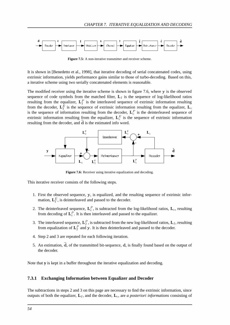
CHAPTER 7. ITERATIVE EQUALIZATION AND DECODING
��������� �� � ����������� ����� ��� ��� � ��� ������������������ �������������� ��� � � � ��� ��� �d c I y I c d
!���"��� ��� ���x
Figure 7.5: A non-iterative transmitter and receiver scheme.
It is shown in [Benedetto et al., 1998], that iterative decoding of serial concatenated codes, usingextrinsic information, yields performance gains similar to those of turbo-decoding. Based on this,a iterative scheme using two serially concatenated elements is reasonable.
The modified receiver using the iterative scheme is shown in figure 7.6, where y is the observedsequence of code symbols from the matched filter, LI is the sequence of log-likelihood ratiosresulting from the equalizer, LPI is the interleaved sequence of extrinsic information resultingfrom the decoder, LEI is the sequence of extrinsic information resulting from the equalizer, Lc
is the sequence of information resulting from the decoder, LPc is the deinterleaved sequence of
extrinsic information resulting from the equalizer, LEc is the sequence of extrinsic information
resulting from the decoder, and d is the estimated info word.
#%$�&('�) * +�,.- /0,�1�2435,.-/6,�* 798�,.-�):,�'<;(,.-
=�798�,.-�):,�'<;(,.-
+-
+
-
EcL cLP
IL
PcLE
ILIL
dy
Figure 7.6: Receiver using iterative equalization and decoding.
This iterative receiver consists of the following steps.
1. First the observed sequence, y, is equalized, and the resulting sequence of extrinsic infor-mation, LEI , is deinterleaved and passed to the decoder.
2. The deinterleaved sequence, LPc , is subtracted from the log-likelihood ratios, Lc, resultingfrom decoding of LPc . It is then interleaved and passed to the equalizer.
3. The interleaved sequence, LPI , is subtracted from the new log-likelihood ratios, LI , resultingfrom equalization of LPI and y. It is then deinterleaved and passed to the decoder.
4. Step 2 and 3 are repeated for each following iteration.
5. An estimation, d, of the transmitted bit-sequence, d, is finally found based on the output ofthe decoder.
Note that y is kept in a buffer throughout the iterative equalization and decoding.
7.3.1 Exchanging Information between Equalizer and Decoder
The subtractions in steps 2 and 3 on this page are necessary to find the extrinsic information, sinceoutputs of both the equalizer, LI , and the decoder, Lc, are a posteriori informations consisting of
54

7.3. ITERATIVE EQUALIZATION AND DECODING
both intrinsic and extrinsic information. The subtractions are due to
LEI = LI − LII (7.6)
= LI − LPI (7.7)
LEc = Lc − LIc (7.8)
= Lc − LPc (7.9)
where LII
is the sequence of intrinsic information of the burst, and LIc is the sequence of intrinsic
information of the code word.
The equalizer in the modified scheme receives two different inputs. The observed sequence fromthe channel, y, and the interleaved extrinsic information from the decoder, LP
I.
The observed sequence, y, is, as described in chapter 6 regarding equalization, used in computingthe branch metrics, which are the log-probability of each branch in the trellis.
The interleaved extrinsic information, LPI
, passed from the decoder, is a log-likelihood ratio ofeach symbol. It can be changed into a log-probability of each branch using the following equations.
logP (Ii = 0) = − log(1 + e
logP (Ii=1)
P (Ii=0)
)(7.10)
logP (Ii = 1) = logP (Ii = 1)
P (Ii = 0)+ logP (Ii = 0) (7.11)
As the two probabilities are only weakly correlated due to the interleaver and the use of extrinsicinformation, they are regarded independent. Therefore the log-probabilities can be added (theprobabilities can be multiplied), and this sum is used in the equalizer.
To preserve information in the iterative loop for each symbol, the Viterbi decoder described inchapter 5, must be modified into a Max-log-MAP decoder like the equalizer was modified inchapter 6. Thereby the extrinsic information can be extracted.
The output of a Max-log-MAP decoder is the log-likelihood ratio of the paths corresponding toeach info bit being 1 compared to the paths corresponding to the info bit being 0. The decoder usedin the implemented iterative scheme must be modified, so the output is the log-likelihood ratio ofthe paths corresponding to each code bit being 1 compared to the paths corresponding to the codebit being 0. As the used encoding has a code rate of 1/2, this means the output of the decoder mustconsist of 456 log-likelihood ratios, one for each code bit, where it previous was 224, one for eachinfo bit (disregarding tail bits). This modification is straightforward, and will not be shown here.
55

CHAPTER 7. ITERATIVE EQUALIZATION AND DECODING
7.4 Simulations and Results
Three performance tests have been conducted:
1. A 4-path quasi-static block Rayleigh fading channel is used as the channel model. The trans-mitter consists of a (23,33) convolutional encoder, an interleaver, and a BPSK modulator.The receiver consists of an iterative equalizer and decoder.This is a test of our considered system model specified in chapter 1.
2. A 4-path fixed channel is used as the channel model. The transmitter and the receiver is thesame as for test 1.This test is an experiment. We wish to investigate the performance if no irrecoverable burstsoccur due to fading in the channel, and if it is possible to achieve a performance gain withmore iterations. The motivation for this experiment is to test the performance the iterativeequalizer and decoder with another channel model scenario.
3. A 4-path quasi-static block Rayleigh fading channel is used as the channel model. The trans-mitter and the receiver is the same as for test 1, except that the interleaver size is increased.This test is another experiment. We wish to investigate the effect of the interleaver size.
7.4.1 Setup for simulations
We wish to investigate the performance by inspecting plots with Bit Error Rate (BER) vs. Eb/N0.We are using Monte Carlo simulations, and for a specified Eb/N0, sequences of 224 bits are trans-mitted through the system until either a predefined number of errors has occurred or a predefinedmaximum number of sequences has been transmitted. The bit error rate is calculated as
BER =# bit errors
# transmitted bits(7.12)
where the number of bit errors is found by comparing the input bits to the system with the outputbits.
The considered (23,33) convolutional encoder converts a info word of 224 info bits and 4 tail bitsinto a code word of 456 bits. The interleaver is the modified GSM interleaver specified in chapter1, and it interleaves the code word of 456 bits over four sequentially transmitted bursts of 114 bits.The BPSK modulator maps the bits in the bursts of {0, 1} into symbols of {−1,+1}.
The symbols from the modulator are transmitted through the specified channel (specified for eachtest). Two channels are considered: 1) The 4-path quasi-static block Rayleigh fading channel,where the coefficients are Rayleigh distributed and time-invariant during one burst of 114 bits, andfor each new burst the coefficients change. 2) The 4-path fixed channel, where the coefficients arefixed to [
√0.45,
√0.25,
√0.15,
√0.15].
After transmission through the channel and a matched filter, the four bursts (corresponding toone code word of 456 bits) are buffered. The equalizer, the deinterleaver, and the decoder isimplemented in an iterative structure, where the equalizer and the decoder are exchanging extrinsicinformation with each other. Both the equalizer and the decoder are based on the Max-log-MAPAlgorithm.
56

7.4. SIMULATIONS AND RESULTS
7.4.2 Tests
Test 1: 4-Path Quasi-Static Block Rayleigh Fading Channel
This test will consider the 4-path quasi-static block Rayleigh fading channel. A large number ofinfo words have been transmitted, and each burst has been transmitted through an individual real-ization of the channel. The results from the simulation using iterative equalization and decodingis shown in figure 7.7.
1 2 3 4 5 6 7 8 910
−6
10−5
10−4
10−3
10−2
10−1
100
Eb/No [dB]
BER
Non−iterative receiver, no encodingNon−iterative receiverIterative receiver, 1 iterationIterative receiver, 2 iterationsIterative receiver, 3 iterationsIterative receiver, 4 iterationsUsing AWGN channel model
Figure 7.7: Performance of the iterative equalization and decoding with transmission through a 4-path quasi-staticblock fading channel.
In the figure we have plotted two curves for comparison with our results. One is the performancefor transmission through the AWGN channel using (23,33) convolutional coding, and it is also thetheoretical lower bound for our results. The other is the performance for transmission through the4-path quasi-static block Rayleigh fading channel and with no coding.
Simulations has shown that there is a performance gain from the 0’th iteration (which is the non-iterative receiver scheme) to the 1’st iteration of 0.7 dB from Eb/N0 = 5.6 dB to 4.9 dB at BER =10−3. The following three iterations (2’nd, 3’rd, and 4’th iteration) do not give any appreciableperformance gain. The results improve only very little compared to the 1’st iteration. At BER =10−2, Eb/N0 is improved from 4.0 dB to 3.3 dB, and at BER = 10−4, Eb/N0 is improved from7.0 dB to 6.3 dB.
In [Jordan et al., 1998] a system model comparable to the one we have implemented, is evaluated.The differences are that [Jordan et al., 1998] have used a "pseudo random" interleaver, a scalingfactor to damp the a priori information to the equalizer, and two different channel models, namelyTypical Urban and Hilly Terrain specified in [Hoeher, 1992]. The results from their simulations forboth channel models show a performance gain of approximately 0.7 dB forBER = 10−3 from thenon-iterative receiver scheme to the 1’st iteration. Furthermore, they do not get any performanceimprovement for the following iterations.
57

CHAPTER 7. ITERATIVE EQUALIZATION AND DECODING
Test 2: 4-Path Fixed Channel
This test will consider a no-fading channel with the fixed coefficients [√
0.45,√
0.25,√
0.15,√0.15]. A large number of info words have been transmitted, and the results from the simulation
is shown in figure 7.8.
1 2 3 4 5 6 7 8 9
10−5
10−4
10−3
10−2
10−1
100
Eb/No [dB]
BE
R
Non−iterative receiver, no encodingNon−iterative receiverIterative receiver, 1 iterationIterative receiver, 2 iterationsIterative receiver, 3 iterationsIterative receiver, 4 iterationsUsing AWGN channel model
Figure 7.8: Performance of the iterative equalization and decoding with transmission through a 4-path fixed channelwith the coefficients [
√0.45,
√0.25,
√0.15,
√0.15].
We have in this figure plotted the lower bound performance curve and the performance for trans-mission through the 4-path fixed channel using no coding for comparison with our results.
The simulations has shown a performance gain for each new iteration from the 0’th iteration to the4’th iteration. EB/N0 is 6.5 dB for the 0’th iteration and 4.5 dB for the 4’th iteration at BER =10−3. The same performance gain of approximately 2 dB is also achieved at BER = 10−2 andBER = 10−4.
In [Jordan et al., 1998] a fixed coefficients channel is also used in their simulations. They usethe five coefficients [
√0.45,
√0.25,
√0.15,
√0.10,
√0.05], where we use only four coefficients,
[√
0.45,√
0.25,√
0.15,√
0.15]. They achieve a performance gain from the 0’th iteration to thefourth iteration is approximately 2 dB at BER= 10−3 with a decreasing performance gain for eachnew iteration.
Test 3: 4-Path Quasi-Static Block Rayleigh Fading Channel and Increased Interleaver Size
This test will consider the 4-path quasi-static block Rayleigh fading channel and an increasedinterleaver size. The simulation setup (and the GSM standard) specify an interleaver size of 456bits, but in this test we use a size of 4104 bits.
58
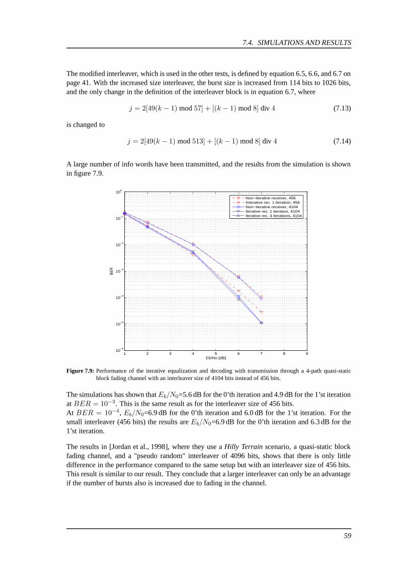
7.4. SIMULATIONS AND RESULTS
The modified interleaver, which is used in the other tests, is defined by equation 6.5, 6.6, and 6.7 onpage 41. With the increased size interleaver, the burst size is increased from 114 bits to 1026 bits,and the only change in the definition of the interleaver block is in equation 6.7, where
j = 2[49(k − 1) mod 57] + [(k − 1) mod 8] div 4 (7.13)
is changed to
j = 2[49(k − 1) mod 513] + [(k − 1) mod 8] div 4 (7.14)
A large number of info words have been transmitted, and the results from the simulation is shownin figure 7.9.
1 2 3 4 5 6 7 8 910
−6
10−5
10−4
10−3
10−2
10−1
100
Eb/No [dB]
BER
Non−iterative receiver, 456Interative rec. 1 iteration, 456Non−iterative receiver, 4104Iterative rec. 1 iteration, 4104Iterative rec. 4 iterations, 4104
Figure 7.9: Performance of the iterative equalization and decoding with transmission through a 4-path quasi-staticblock fading channel with an interleaver size of 4104 bits instead of 456 bits.
The simulations has shown thatEb/N0=5.6 dB for the 0’th iteration and 4.9 dB for the 1’st iterationat BER = 10−3. This is the same result as for the interleaver size of 456 bits.At BER = 10−4, Eb/N0=6.9 dB for the 0’th iteration and 6.0 dB for the 1’st iteration. For thesmall interleaver (456 bits) the results are Eb/N0=6.9 dB for the 0’th iteration and 6.3 dB for the1’st iteration.
The results in [Jordan et al., 1998], where they use a Hilly Terrain scenario, a quasi-static blockfading channel, and a "pseudo random" interleaver of 4096 bits, shows that there is only littledifference in the performance compared to the same setup but with an interleaver size of 456 bits.This result is similar to our result. They conclude that a larger interleaver can only be an advantageif the number of bursts also is increased due to fading in the channel.
59

CHAPTER 7. ITERATIVE EQUALIZATION AND DECODING
7.4.3 Effect of Our Assumptions and Constraints
GMSK. In this project BPSK modulation is considered, while the GSM specifications considersGMSK modulation. GMSK itself can introduce ISI in the system.
Multiuser. Multiuser detection is not considered in this project. As time division is used in theGSM specifications, the effect of having several users has effect on the transmission rate, and itgives interference from other users at same frequency.
Hardware Signal Processing. The sampling process and other hardware signal processing pro-cesses are omitted in this project. A discrete time baseband representation of the transmitted signalis used. In physical systems, these hardware processes exist, thus adding noise to the system. Ad-ditive white Gaussian noise is incorporated in our system to represent thermal noise, but we shouldbe aware that this is not a representation of all the noise from the hardware.
Channel Estimation. Instead of estimating the channel characteristics, perfect knowledge ofthe channel is assumed to be known in our project. This raises the performance of the receiver, asequalization always is based on estimated or known channel characteristics.
Time-Variant Channel Characteristics. The channel considered in this system is time-invariantfor each transmitted burst. In real applications this is not the case. Equalization is not based on theoptimal channel characteristics, thereby lowering the performance of the receiver.
Class 1 and 2 bits. According to GSM specifications, we should only encode part of the infoword, but we encode the entire info word, and that must give better performance than that of asystem true to the GSM specifications, as uncoded bits give worse performance than coded bits.
The "real" GSM Interleaver. The interleaver specified in the GSM specifications interleaveseach code word together with the preceding and succeeding code words. This is not used in ourproject, but use of this interleaver would probably increase the performance, as the errors aredistributed over several code words.
60

CHAPTER
Conclusion 8Summary
The aim of this project is to improve a GSM receiver by using iterative equalization and decoding.Due to the time constraint we have restricted our system model to:
• A (23,33) convolutional channel encoder.
• An interleaver + burst assembler.
• A BPSK modulator (or mapper).
• A quasi-static tapped delay line channel model.
• An iterative equalizer and decoder.
The (23,33) convolutional encoder is the same as the one specified in the GSM standard, exceptthat we do not distinguish class 1, class 2, and parity bits. We consider an incoming sequence,the info word, of 224 bits and add 4 tail bits. The encoded sequence, the code word, is of length456 bits, as the GSM code word.
The considered interleaver is a modified version of the one specified in the GSM standard. Insteadof interleaving one code word of 456 bits over 8 sequentially transmitted bursts in 16 half burstsof 57 bits, the modified interleaver interleaves one code word over only 4 sequentially transmittedbursts in 4 full bursts of 114 bits. By doing this, the interleaver blocks only contain code bits fromone code word instead of two.
A tapped delay line model is used to model the time-variant multipath channel. We considerboth fixed coefficients and Rayleigh distributed coefficients. The channel is quasi-static, meaningthat the coefficients are time-invariant during one burst of 114 bits, and for each new burst thecoefficients change.
A bank of matched filters are applied to the received signal. The output of the matched filters,which is four bursts (corresponding to one code word of 456 bits), is buffered. The equalizer, thedeinterleaver, and the decoder is implemented in an iterative structure, where the equalizer and thedecoder are exchanging extrinsic information with each other. Both the equalizer and the decoderare based on the Max-log-MAP Algorithm. Hard-decision is made on the output of the decoderafter the last iteration.
61

CHAPTER 8. CONCLUSION
Results
We will conclude on three performance results:
1. The considered model with Rayleigh fading channel. This will be the conclusion on our aimin this project.
2. The considered model with no-fading channel (fixed coefficients).
3. The considered model with Rayleigh fading channel, but where the interleaver size is in-creased from 456 bits to 4104 bits.
1. Simulations has shown that there is a performance gain from the 0’th iteration (which is thenon-iterative receiver scheme) to the 1’st iteration fromEb/N0 = 5.6 dB to 4.9 dB atBER = 10−3.The following three iterations (2’nd, 3’rd, and 4’th iteration) do not give any appreciable perfor-mance gain. The results improve only very little compared to the 1’st iteration. At BER = 10−2,Eb/N0 is improved from 4.0 dB to 3.3 dB, and at BER = 10−4, Eb/N0 is improved from 7.0 dBto 6.3 dB. These results show that there is an improvement by using iterative equalization and de-coding in the receiver in a GSM system, with the assumptions and constraints made in our systemmodel.It should be noted that it is only relevant to use the 0’th and the 1’st iteration. The rest are unnec-essary, so to reduce complexity when considering implementation in an application, only the 0’thand the 1’st iteration should be considered.
2. An experiment, where the coefficients in the channel are fixed to [√
0.45,√
0.25,√
0.15,√0.15], has shown a performance gain for each new iteration from the 0’th iteration to the 4’th
iteration. EB/N0 is 6.5 dB for the 0’th iteration and 4.5 dB for the 4’th iteration at BER = 10−3.The same performance gain of approximately 2 dB is also achieved at BER = 10−2 and BER =10−4.This experiment is conducted to show, that the performance will increase for every new iterationfrom the 0’th iteration to the 4’th iteration, if we fix the coefficients so no fading will occur andnone of the bursts are irrecoverable.
3. Another experiment, where the interleaver size is increased from 456 bits to 4104 bits hasshown that Eb/N0=5.6 dB for the 0’th iteration and 4.9 dB for the 1’st iteration at BER = 10−3.This is the same result as for the interleaver size of 456 bits.At BER = 10−4, Eb/N0=6.9 dB for the 0’th iteration and 6.0 dB for the 1’st iteration. For thesmall interleaver (456 bits) the results are Eb/N0=6.9 dB for the 0’th iteration and 6.3 dB for the1’st iteration.From these results we can conclude, that there is a small improvement at high SNR, and there isno improvement at low SNR, when using an interleaver size of 4104 bits instead of 456 bits. Wecan also conclude, that in most cases it is not advisable to increase the interleaver size consideringthe rather modest performance gain archived compared to the increased time complexity.
62

Perspectives
If the iterative equalization and decoding scheme were to be implemented in a physical GSMsystem, some aspects were needed to be investigated:
• The "real" GSM interleaver and burst assembler should be implemented, and the perfor-mance should be tested.
• The GMSK modulation scheme should be implemented, and the performance should betested.
• The code word structure, where only class 1 bits are encoded and class 2 bits are uncoded,should be implemented, and the performance should be tested.
Even though the above aspects will influence the performance of the iterative receiver, we wouldstill expect an improvement in the performance, if the iterative equalization and decoding schemewere implemented in a GSM receiver.
Another interesting investigation would be to implement the iterative equalization and decodingscheme in an EDGE system, which is an upgrade of the GSM system. The difference betweenthe GSM system and the EDGE system is the modulation scheme. EDGE uses 8-PSK instead ofGMSK, and this would probably give a bigger gain in the performance due to the higher ordermodulation scheme.
63


APPENDIX
Implementation AA block diagram of the implemented system is shown in figure A.1.
������� ������ ������ ���������
� ������������������
� �! �"��#�$�"�&%('���!)�������
� *�����+�#���������
,.-)/ ���1032)��� 4 /�5�5 ���
6 "�7�����8:9 -)/ ��9+0#";9����<��0#= �#���> 5 ���01 �$
�8��� � ����?
@A�����8��!� 5 01� ���!�
4 '.B*C@D��� / �#���#��
E F G H
I
JLKMJNKMO
J K PMOJRQ PMOJ(Q PM
J Q MOE S T ��"0U ����!������������� V
V W
W
Figure A.1: Block diagram of the system model.
The flow of the system (corresponding to one realization) is the following:
1. Four different channel models, a1, a2, a3, and a4 (one for each burst), are generated with 4Rayleigh distributed coefficients. Then AWGN is added and the matched filter is applied.
2. An info word, d ∈ {0, 1}, containing 224 bits, is created randomly.
3. The info word is encoded, using the (23,33) convolutional encoder, into a code word, c, oflength 456.
4. The code word is interleaved and separated into 4 bursts, I1, I2, I3, and I4.
65
APPENDIX A. IMPLEMENTATION
5. Ik, where k = {1, 2, 3, 4}, is mapped onto a baseband representation of BPSK-symbols, xk.
6. xk is, using channel model ak, distorted into the observed sequence yk.
7. yk is equalized in the Max-log-MAP equalizer, resulting in a sequence of a priori informa-tion, LIK .
8. LI1 , LI2 , LI3 , and LI4 are deinterleaved and merged into the sequence LPc of length 456.
9. This sequence is decoded in the Max-log-MAP decoder, resulting in the sequence Lc.
10. LPc is subtracted, giving the extrinsic information LEc .
11. The interleaver interleaves and splits LEc into 4 bursts, LPI1 , LPI2 , LPI3 , and LPI4 , each of
length 114.
12. LPIk , for k = {1, 2, 3, 4}, are, together with yk, used as input to the equalizer, resulting in
new sequences of information, LIk .
13. LPIk is subtracted, giving the extrinsic information LE
Ik .
14. LEI1 , LEI2 , LEI3 , and LEI4 are deinterleaved and merged into the sequence LPc .
15. Steps 9-14 are repeated for each preceding iteration.
16. Finally hard decision is made based on the output of the decoder, resulting in an estimatedinfo word, d of length 224.
Note that the buffer shown in the figure is not implemented as a separate function, but in the waythat yk for k = {1, 2, 3, 4} is stored throughout all the iterations.
In the following the implementation of each block (except the buffer) in figure A.1 will be de-scribed.
A.1 (23,33) Convolutional Encoder
The purpose of the convolutional encoder is to encode an info word. The convolutional encoder isdescribed in chapter 4
Input
• An info word, d, of length m
Output
• A code word, c, of length 2(m+ 4)
66

A.2. INTERLEAVER
The encoder is initialized to zero-state, meaning di = 0 for i ≤ 0.
Four zero-bits are added to the end of the info word to reset the encoder and terminate the trellisin the decoder.
d• = {d1, d2, ..., dm, 0, 0, 0, 0} (A.1)
The encoder is, according the GSM standard, a rate 12 convolutional encoder defined by the poly-
nomials
g1 = 1 +D3 +D4 (A.2)
g2 = 1 +D +D3 +D4 (A.3)
It is implemented using the following equations
c2i−1 = d•i ⊕ d•i−3 ⊕ d•i−4 (A.4)
c2i = d•i ⊕ d•i−1 ⊕ d•i−3 ⊕ d•i−4 (A.5)
for i = 1, 2, ...,m.
A.2 Interleaver
The interleaver interleaves the code word and splits it up into 4 bursts.
Input
• A code word, c, of length 456.
Output
• Four bursts, I1, I2, I3, and I4, each of length 114.
The interleaver in GSM-systems is specified by
IBj = cm,k for k = 1, 2, . . . , 456 (A.6)
where
m = 1, 2, . . . (A.7)
B = B0 + 4m+ ([k − 1] mod 8) (A.8)
j = 2[(49[k − 1]) mod 57] + [([k − 1] mod 8) div 4] (A.9)
where B is the burst number, j is the bit number in burst B, m is the sequence number of thecoded bits, and k is the bit number in the coded bits sequence m.
67

APPENDIX A. IMPLEMENTATION
This GSM-specified interleaver interleaves each code word into 8 bursts, where the first 4 containsome of the preceding code word, and the last 4 also contain some of the succeeding code word.As this is unwanted due to the iterative receiver, some slight modifications have been made. Onlyone code word is considered, and it is being interleaved into only 4 bursts.
IBj = ck for k = 1, 2, . . . , 456 (A.10)
where
B = ([k − 1] mod 4) + 1 (A.11)
j = 2[(49[k − 1]) mod 57] + [([k − 1] mod 8) div 4] (A.12)
where B ∈ {1, 2, 3, 4} is the burst number, j ∈ {1, 2, . . . , 114} is the bit number in burst B, andk is the bit number in the code word c.
The outcome of interleaving the code word c = {0, 1, 2, ..., 455} is shown in table A.2 on thefacing page.
A.3 BPSK Modulator
The purpose of the modulator is to map the code word into the corresponding baseband represen-tation of BPSK. The function is described in chapter 3.
Input
• An interleaved code word, I, of length m
Output
• A baseband representation, x, of length m
The modulator maps the received code bits to modulated symbols
xi =
{+1 for Ii = 1
−1 for Ii = 0(A.13)
It is implemented using the following equation
xi = (Ii − 0.5) · 2 for i = 1, 2, ...,m (A.14)
68

A.3. BPSK MODULATOR
Burst 1 2 3 4
j
0 0 57 114 171
1 228 285 342 399
2 64 121 178 235
3 292 349 406 7
4 128 185 242 299
5 356 413 14 71
6 196 249 306 363
7 420 21 78 135
8 256 313 370 427
9 28 85 142 199
10 320 377 434 35
11 92 149 206 263
12 384 441 42 99
13 156 213 270 327
14 448 49 106 163
15 220 277 334 391
16 56 113 170 227
17 284 341 398 455
18 120 177 234 291
19 348 405 6 63
20 184 241 298 355
21 412 13 70 127
22 248 305 362 419
23 20 77 134 191
24 312 369 426 27
25 84 141 198 255
26 376 433 34 91
27 148 205 262 319
28 440 41 98 155
29 212 269 326 383
30 48 105 162 219
31 276 333 390 447
32 112 169 226 283
33 340 397 454 55
34 176 233 290 347
35 404 5 62 119
36 240 297 354 411
37 12 69 126 183
38 304 361 418 19
39 76 133 190 247
40 368 425 26 83
41 140 197 254 311
42 432 33 90 147
43 204 261 318 375
44 40 97 154 211
45 268 325 382 439
46 104 161 218 275
47 332 389 446 47
48 168 225 282 339
49 396 453 54 111
50 232 289 346 403
51 4 61 118 175
52 296 353 410 11
53 68 125 182 239
54 360 417 18 75
55 132 189 246 303
56 424 25 85 139
Burst 1 2 3 4
j
57 196 253 310 367
58 32 89 146 203
59 260 317 374 431
60 96 153 210 267
61 324 381 438 39
62 160 217 274 331
63 388 445 46 103
64 224 281 338 395
65 452 53 110 167
66 288 345 402 3
67 60 117 174 231
68 352 409 10 67
69 124 181 238 295
70 416 17 74 131
71 188 245 302 359
72 24 81 138 195
73 252 309 366 423
74 88 145 202 259
75 316 373 430 31
76 152 209 266 323
77 380 437 37 95
78 216 273 330 387
79 444 45 102 159
80 280 337 394 451
81 52 109 166 223
82 344 401 2 59
83 116 173 230 287
84 408 9 66 123
85 180 237 294 351
86 16 73 130 187
87 244 301 358 415
88 80 137 194 251
89 308 365 422 23
90 144 201 258 315
91 372 429 30 87
92 208 265 322 379
93 436 37 94 151
94 272 329 386 443
95 44 101 158 215
96 336 393 450 51
97 108 165 222 279
98 400 1 58 115
99 172 229 286 343
100 8 65 122 179
101 236 293 350 407
102 72 129 186 243
103 300 357 414 15
104 136 193 250 307
105 364 421 22 79
106 200 257 314 371
107 428 29 86 143
108 264 321 378 435
109 36 93 150 207
110 328 385 442 43
111 100 157 214 271
112 392 449 50 107
113 164 221 278 335
Figure A.2: The outcome of interleaving the code word c = {0, 1, 2, ..., 455}.
69

APPENDIX A. IMPLEMENTATION
A.4 4-Paths Quasi-static Block Fading Channel
The purpose of the channel is to distort the transmitted signal. The channel is described in chapter2.
Input
• A baseband representation of BPSK-modulated symbols, x, of length m.
• The channel coefficients, a1, a2, a3 and a4. Each al is generated as: al = zl,1 + j · zl,2,where zl,1 and zl,2 are realizations of a white Gaussian random process with zero-mean andvariance 1.
• The signal-to-noise ratio, Eb
N0.
• The code rate, Rc.
Output
• A baseband representation of distorted BPSK-modulated symbols, y, of length m.
The channel is shown in figure A.3.
�����
���
�
�
�
��� �� �� ���
�
�� �� ��� �� � �� ��
� ���� ���� ��� � ���
� ���� ���� ���� ���
� ���
� ���
Figure A.3: Block diagram a 4-paths quasi-static block fading channel.
The channel and the corresponding matched filter is implemented as described in section 2.3.
y = R x+AH n (A.15)
70

A.4. 4-PATHS QUASI-STATIC BLOCK FADING CHANNEL
where n is a vector containing realizations of the white Gaussian noise variable N , R = AH Aand
AH =
a∗1 a∗2 a∗3 · · · a∗L 0 0 · · ·0 a∗1 a∗2 a∗3 · · · a∗L 0 · · ·0 0 a∗1 a∗2 a∗3 · · · a∗L · · ·...
......
. . . . . . . . . . . . . . .
(A.16)
where a1, a2 etc. are channel taps. Note that the sequences x and y are represented as vectors.
A.4.1 Generating the Additive White Gaussian Noise
N can be generated as
N = σn · (ZRe + j · ZIm) (A.17)
where σn is the standard deviation of the noise, and ZRe and ZIm are normal distributed randomprocesses with variance 1 and zero mean.
The noise variance is dependent of the SNR, which can be expressed as
SNR =2EsN0
= 2RcEbN0
(A.18)
where Es is the energy in each symbol after encoding, and Rc is the coding rate. The expressionin equation A.18 is derived in subsection 2.3 on page 18.
SNR is also the ratio between the signal variance and the noise variance
SNR =σ2s
σ2n
(A.19)
and since σ2s = E[x2] = 1, the noise variance can be derived from equation A.18 and A.19 as
SNR = 2Rc ·EbN0
=σ2s
σ2n
(A.20)
⇓σ2n =
1
2Rc · Eb
N0
(A.21)
The white Gaussian noise variable from equation A.17 is then described as
N = σn · (ZRe + j · ZIm) =
√1
2Rc · Eb
N0
· (ZRe + j · ZIm) (A.22)
71
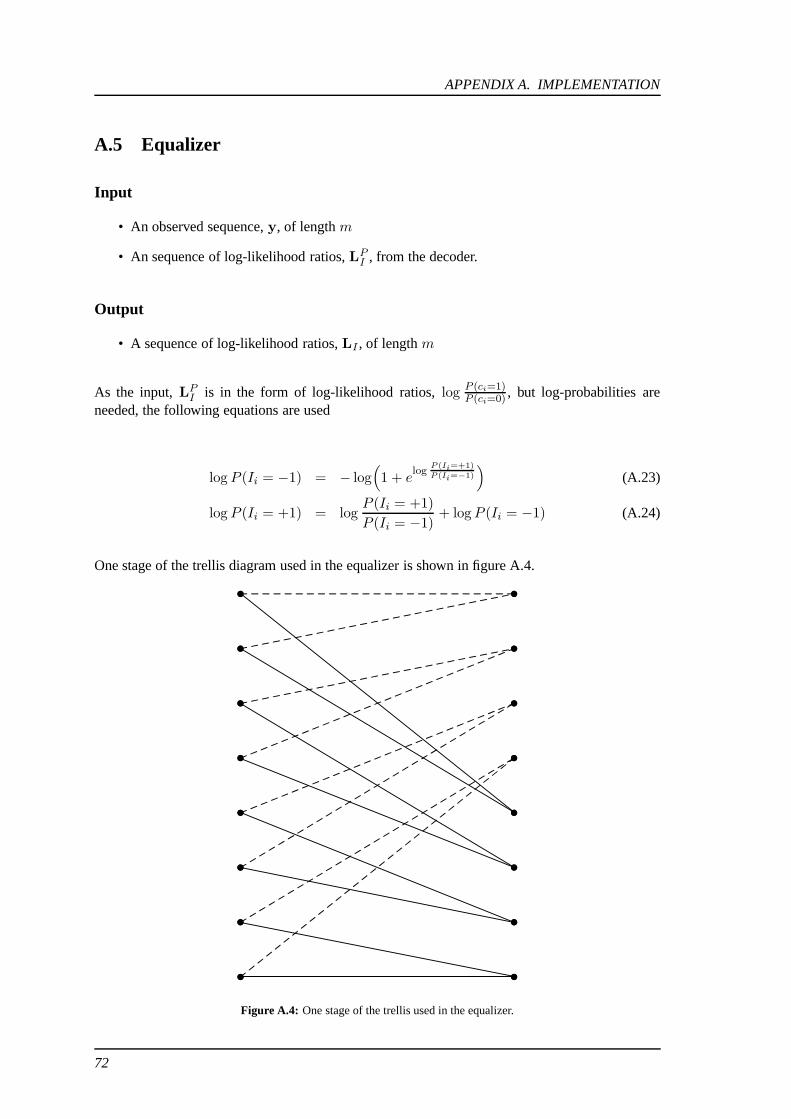
APPENDIX A. IMPLEMENTATION
A.5 Equalizer
Input
• An observed sequence, y, of length m
• An sequence of log-likelihood ratios, LPI , from the decoder.
Output
• A sequence of log-likelihood ratios, LI , of length m
As the input, LPI is in the form of log-likelihood ratios, log P (ci=1)P (ci=0) , but log-probabilities are
needed, the following equations are used
log P (Ii = −1) = − log(1 + e
logP (Ii=+1)
P (Ii=−1)
)(A.23)
log P (Ii = +1) = logP (Ii = +1)
P (Ii = −1)+ logP (Ii = −1) (A.24)
One stage of the trellis diagram used in the equalizer is shown in figure A.4.
Figure A.4: One stage of the trellis used in the equalizer.
72

A.5. EQUALIZER
The following equations is derived in chapter 6 as the log-probability of a given branch in thetrellis, depending on the observed sequence y.
γ′k(i) = −σ−1n · Re(uk · (Σi−1
j=1%i,j · uj − yi)) (A.25)
This gives, using figure A.4, the following equations
γ′1(i) = −σ−1n Re(+%1,2 + %1,3 + %1,4 + yi) + logP (Ii = −1) (A.26)
γ′2(i) = −σ−1n Re(−%1,2 − %1,3 − %1,4 − yi) + logP (Ii = +1) (A.27)
γ′3(i) = −σ−1n Re(+%1,2 + %1,3 − %1,4 + yi) + logP (Ii = −1) (A.28)
γ′4(i) = −σ−1n Re(−%1,2 − %1,3 + %1,4 − yi) + logP (Ii = +1) (A.29)
γ′5(i) = −σ−1n Re(+%1,2 − %1,3 + %1,4 + yi) + logP (Ii = −1) (A.30)
γ′6(i) = −σ−1n Re(−%1,2 + %1,3 − %1,4 − yi) + logP (Ii = +1) (A.31)
γ′7(i) = −σ−1n Re(+%1,2 − %1,3 − %1,4 + yi) + logP (Ii = −1) (A.32)
γ′8(i) = −σ−1n Re(−%1,2 + %1,3 + %1,4 − yi) + logP (Ii = +1) (A.33)
γ′9(i) = −σ−1n Re(−%1,2 + %1,3 + %1,4 + yi) + logP (Ii = −1) (A.34)
γ′10(i) = −σ−1n Re(+%1,2 − %1,3 − %1,4 − yi) + logP (Ii = +1) (A.35)
γ′11(i) = −σ−1n Re(−%1,2 + %1,3 − %1,4 + yi) + logP (Ii = −1) (A.36)
γ′12(i) = −σ−1n Re(+%1,2 − %1,3 + %1,4 − yi) + logP (Ii = +1) (A.37)
γ′13(i) = −σ−1n Re(−%1,2 − %1,3 + %1,4 + yi) + logP (Ii = −1) (A.38)
γ′14(i) = −σ−1n Re(+%1,2 + %1,3 − %1,4 − yi) + logP (Ii = +1) (A.39)
γ′15(i) = −σ−1n Re(−%1,2 − %1,3 − %1,4 + yi) + logP (Ii = −1) (A.40)
γ′16(i) = −σ−1n Re(+%1,2 + %1,3 + %1,4 − yi) + logP (Ii = +1) (A.41)
for i = 1, 2, ...,m
From section 6.4 we have, that
α′uk
(i) = maxj
[α′uj
(i− 1) + γ′uj ,uk(i− 1)
](A.42)
β′uk(i) = max
j
[β′uj
(i+ 1) + γ′uk,uj(i)]
(A.43)
where uk and uj are states in the trellis.
This gives, when using figure A.4, the following equations
α′1(i) = max[α′
1(i− 1) + γ′1(i− 1), α′2(i− 1) + γ′3(i− 1)] (A.44)
α′2(i) = max[α′
3(i− 1) + γ′5(i− 1), α′4(i− 1) + γ′7(i− 1)] (A.45)
α′3(i) = max[α′
5(i− 1) + γ′9(i− 1), α′6(i− 1) + γ′11(i− 1)] (A.46)
α′4(i) = max[α′
7(i− 1) + γ′13(i− 1), α′8(i− 1) + γ′15(i− 1)] (A.47)
α′5(i) = max[α′
1(i− 1) + γ′2(i− 1), α′2(i− 1) + γ′4(i− 1)] (A.48)
α′6(i) = max[α′
3(i− 1) + γ′6(i− 1), α′4(i− 1) + γ′8(i− 1)] (A.49)
α′7(i) = max[α′
5(i− 1) + γ′10(i− 1), α′6(i− 1) + γ′12(i− 1)] (A.50)
α′8(i) = max[α′
7(i− 1) + γ′14(i− 1), α′8(i− 1) + γ′16(i− 1)] (A.51)
for i = 2, 3, ...,m + 1
73

APPENDIX A. IMPLEMENTATION
β′1(i) = max[β ′1(i+ 1) + γ′1(i), β
′5(i+ 1) + γ′2(i)] (A.52)
β′2(i) = max[β ′1(i+ 1) + γ′3(i), β
′5(i+ 1) + γ′4(i)] (A.53)
β′3(i) = max[β ′2(i+ 1) + γ′5(i), β
′6(i+ 1) + γ′6(i)] (A.54)
β′4(i) = max[β ′2(i+ 1) + γ′7(i), β
′6(i+ 1) + γ′8(i)] (A.55)
β′5(i) = max[β ′3(i+ 1) + γ′9(i), β
′7(i+ 1) + γ′10(i)] (A.56)
β′6(i) = max[β ′3(i+ 1) + γ′11(i), β
′7(i+ 1) + γ′12(i)] (A.57)
β′7(i) = max[β ′4(i+ 1) + γ′13(i), β
′8(i+ 1) + γ′14(i)] (A.58)
β′8(i) = max[β ′4(i+ 1) + γ′15(i), β
′8(i+ 1) + γ′16(i)] (A.59)
for i = m,m− 1, ..., 1
Now that γ ′’s, α′’s and β′’s are known, we can find the log-probability, δ ′, of each branch, basedon the entire sequence of code symbols.
δ′uk,uj(i) = α′
uk(i) + γ′uk,uj
(i) + β′uj
(i+ 1) (A.60)
This gives the following equations
δ1(i) = max[α′1(i) + γ′1(i) + β′
1(i+ 1), α′2(i) + γ′3(i) + β′
1(i+ 1)] (A.61)
δ2(i) = max[α′3(i) + γ′5(i) + β′
2(i+ 1), α′4(i) + γ′7(i) + β′
2(i+ 1)] (A.62)
δ3(i) = max[α′5(i) + γ′9(i) + β′
3(i+ 1), α′6(i) + γ′11(i) + β′
3(i+ 1)] (A.63)
δ4(i) = max[α′7(i) + γ′13(i) + β′
4(i+ 1), α′8(i) + γ′15(i) + β′
4(i+ 1)] (A.64)
δ5(i) = max[α′1(i) + γ′2(i) + β′
5(i+ 1), α′2(i) + γ′4(i) + β′
5(i+ 1)] (A.65)
δ6(i) = max[α′3(i) + γ′6(i) + β′
6(i+ 1), α′4(i) + γ′8(i) + β′
6(i+ 1)] (A.66)
δ7(i) = max[α′5(i) + γ′10(i) + β′
7(i+ 1), α′6(i) + γ′12(i) + β′
7(i+ 1)] (A.67)
δ8(i) = max[α′7(i) + γ′14(i) + β′
8(i+ 1), α′8(i) + γ′16(i) + β′
8(i+ 1)] (A.68)
for i = 1, 2, ...,m
The output, LI , is calculated as
LI(i) = max[δ5(i), δ6(i), δ7(i), δ8(i)] − max[δ1(i), δ2(i), δ3(i), δ4(i)] (A.69)
where i = {1, 2, ...,m} and as the branches number 5, 6, 7, and 8 corresponds to di = 1, andbranches number 1, 2, 3, 4 corresponds to di = 0.
A.6 Deinterleaver
The purpose of the deinterleaver is to merge and deinterleave 4 burst into one code word. Thefunction is the inverse of that described in section A.2.
Input
• 4 bursts, IE,1I , IE,2I , IE,3I and IE,4I , each of length 114.
74

A.7. MAX-LOG-MAP DECODER
Output
• A code word, Lpc , of length 456.
The function is implemented using the following equation
ck = IBj for k = 1, 2, . . . , 456 (A.70)
where
B = ([k − 1] mod 4) + 1 (A.71)
j = 2[(49[k − 1]) mod 57] + [([k − 1] mod 8) div 4] (A.72)
where B is the burst number, j is the bit number in burst B, and k is the bit number in the codeword.
A.7 Max-log-MAP Decoder
The purpose of the Max-log-MAP decoder is to decode the received code word. The function of aViterbi decoder is described is chapter 5, and the Max-log-MAP algorithm is described is chapter6.
Input
• Log-likelihood ratios LPc of a code word of length 2m+ 8
Output
• Log-likelihood ratios Lc of a code word of length 2m+ 8
• Log-likelihood ratios Ld of an info word of length m
The convolutional encoder consists of 4 memory elements. This leads to 16 states. The diagramfor one stage in the Trellis diagram is shown in figure A.5.
As the input is in the form of log-likelihood ratios, log P (ci=1)P (ci=0) , but what is needed is log-
probabilities, the following equations are used
logP (ci = 0) = − log(1 + e
logP (ci=1)
P (ci=0)
)(A.73)
logP (ci = 1) = logP (ci = 1)
P (ci = 0)+ log P (ci = 0) (A.74)
In the Max-log-MAP algorithm, the branch metric, γk,j(i), is the log-probability of the branch,Since we now have the probabilities of each of the symbols, corresponding to each branch, and we
75

APPENDIX A. IMPLEMENTATION
consider these probabilities independent, the log-probability of a given branch is the sum of theselog-probabilities.
γ′1(i) = logP (c2i−1 = 0) + logP (c2i = 0) (A.75)
γ′2(i) = logP (c2i−1 = 1) + logP (c2i = 1) (A.76)
γ′3(i) = logP (c2i−1 = 1) + logP (c2i = 1) (A.77)
γ′4(i) = logP (c2i−1 = 0) + logP (c2i = 0) (A.78)
γ′5(i) = logP (c2i−1 = 1) + logP (c2i = 1) (A.79)
γ′6(i) = logP (c2i−1 = 0) + logP (c2i = 0) (A.80)
γ′7(i) = logP (c2i−1 = 0) + logP (c2i = 0) (A.81)
γ′8(i) = logP (c2i−1 = 1) + logP (c2i = 1) (A.82)
γ′9(i) = logP (c2i−1 = 0) + logP (c2i = 0) (A.83)
γ′10(i) = logP (c2i−1 = 1) + logP (c2i = 1) (A.84)
γ′11(i) = logP (c2i−1 = 1) + logP (c2i = 1) (A.85)
γ′12(i) = logP (c2i−1 = 0) + logP (c2i = 0) (A.86)
γ′13(i) = logP (c2i−1 = 1) + logP (c2i = 1) (A.87)
γ′14(i) = logP (c2i−1 = 0) + logP (c2i = 0) (A.88)
γ′15(i) = logP (c2i−1 = 0) + logP (c2i = 0) (A.89)
γ′16(i) = logP (c2i−1 = 1) + logP (c2i = 1) (A.90)
γ′17(i) = logP (c2i−1 = 0) + logP (c2i = 1) (A.91)
γ′18(i) = logP (c2i−1 = 1) + logP (c2i = 0) (A.92)
γ′19(i) = logP (c2i−1 = 1) + logP (c2i = 0) (A.93)
γ′20(i) = logP (c2i−1 = 0) + logP (c2i = 1) (A.94)
γ′21(i) = logP (c2i−1 = 1) + logP (c2i = 0) (A.95)
γ′22(i) = logP (c2i−1 = 0) + logP (c2i = 1) (A.96)
γ′23(i) = logP (c2i−1 = 0) + logP (c2i = 1) (A.97)
γ′24(i) = logP (c2i−1 = 1) + logP (c2i = 0) (A.98)
γ′25(i) = logP (c2i−1 = 0) + logP (c2i = 1) (A.99)
γ′26(i) = logP (c2i−1 = 1) + logP (c2i = 0) (A.100)
γ′27(i) = logP (c2i−1 = 1) + logP (c2i = 0) (A.101)
γ′28(i) = logP (c2i−1 = 0) + logP (c2i = 1) (A.102)
γ′29(i) = logP (c2i−1 = 1) + logP (c2i = 0) (A.103)
γ′30(i) = logP (c2i−1 = 0) + logP (c2i = 1) (A.104)
γ′31(i) = logP (c2i−1 = 0) + logP (c2i = 1) (A.105)
γ′32(i) = logP (c2i−1 = 1) + logP (c2i = 0) (A.106)
where i = {1, 2, ...,m + 4}
76

A.7. MAX-LOG-MAP DECODER
From section 6.4 we have, that
α′uk
(i) = maxj
[α′uj
(i− 1) + γ′uj ,uk(i− 1)
](A.107)
β′uk(i) = max
j
[β′uj
(i+ 1) + γ′uk,uj(i)]
(A.108)
where uk and uj are states in the trellis.
This gives, when using figure A.5, the following equations
α′1(i+ 1) = max[α′
1(i) + γ′1(i), α′2(i) + γ′3(i)] (A.109)
α′2(i+ 1) = max[α′
3(i) + γ′5(i), α′4(i) + γ′7(i)] (A.110)
α′3(i+ 1) = max[α′
5(i) + γ′9(i), α′6(i) + γ′11(i)] (A.111)
α′4(i+ 1) = max[α′
7(i) + γ′13(i), α′8(i) + γ′15(i)] (A.112)
α′5(i+ 1) = max[α′
9(i) + γ′17(i), α′10(i) + γ′19(i)] (A.113)
α′6(i+ 1) = max[α′
11(i) + γ′21(i), α′12(i) + γ′23(i)] (A.114)
α′7(i+ 1) = max[α′
13(i) + γ′25(i), α′14(i) + γ′27(i)] (A.115)
α′8(i+ 1) = max[α′
15(i) + γ′29(i), α′16(i) + γ′31(i)] (A.116)
α′9(i+ 1) = max[α′
1(i) + γ′2(i), α′2(i) + γ′4(i)] (A.117)
α′10(i+ 1) = max[α′
3(i) + γ′6(i), α′4(i) + γ′8(i)] (A.118)
α′11(i+ 1) = max[α′
5(i) + γ′10(i), α′6(i) + γ′12(i)] (A.119)
α′12(i+ 1) = max[α′
7(i) + γ′14(i), α′8(i) + γ′16(i)] (A.120)
α′13(i+ 1) = max[α′
9(i) + γ′18(i), α′10(i) + γ′20(i)] (A.121)
α′14(i+ 1) = max[α′
11(i) + γ′22(i), α′12(i) + γ′24(i)] (A.122)
α′15(i+ 1) = max[α′
13(i) + γ′26(i), α′14(i) + γ′28(i)] (A.123)
α′16(i+ 1) = max[α′
15(i) + γ′30(i), α′16(i) + γ′32(i)] (A.124)
where i = {1, 2, ...,m + 4}
77

APPENDIX A. IMPLEMENTATION
β′1(i) = max[β ′1(i+ 1) + γ′1(i), β
′9(i+ 1) + γ′2(i)] (A.125)
β′2(i) = max[β ′1(i+ 1) + γ′3(i), β
′9(i+ 1) + γ′4(i)] (A.126)
β′3(i) = max[β ′2(i+ 1) + γ′5(i), β
′10(i+ 1) + γ′6(i)] (A.127)
β′4(i) = max[β ′2(i+ 1) + γ′7(i), β
′10(i+ 1) + γ′8(i)] (A.128)
β′5(i) = max[β ′3(i+ 1) + γ′9(i), β
′11(i+ 1) + γ′10(i)] (A.129)
β′6(i) = max[β ′3(i+ 1) + γ′11(i), β
′11(i+ 1) + γ′12(i)] (A.130)
β′7(i) = max[β ′4(i+ 1) + γ′13(i), β
′12(i+ 1) + γ′14(i)] (A.131)
β′8(i) = max[β ′4(i+ 1) + γ′15(i), β
′12(i+ 1) + γ′16(i)] (A.132)
β′9(i) = max[β ′5(i+ 1) + γ′17(i), β
′13(i+ 1) + γ′18(i)] (A.133)
β′10(i) = max[β ′5(i+ 1) + γ′19(i), β
′13(i+ 1) + γ′20(i)] (A.134)
β′11(i) = max[β ′6(i+ 1) + γ′21(i), β
′14(i+ 1) + γ′22(i)] (A.135)
β′12(i) = max[β ′6(i+ 1) + γ′23(i), β
′14(i+ 1) + γ′24(i)] (A.136)
β′13(i) = max[β ′7(i+ 1) + γ′25(i), β
′15(i+ 1) + γ′26(i)] (A.137)
β′14(i) = max[β ′7(i+ 1) + γ′27(i), β
′15(i+ 1) + γ′28(i)] (A.138)
β′15(i) = max[β ′8(i+ 1) + γ′29(i), β
′16(i+ 1) + γ′30(i)] (A.139)
β′16(i) = max[β ′8(i+ 1) + γ′31(i), β
′16(i+ 1) + γ′32(i)] (A.140)
where i = {m+ 4,m+ 3, ..., 1}
Now that γ ′’s, α′’s and β′’s are known, we can find the log-probability, δ ′uk,uj, of each branch,
based on the entire sequence of code symbols.
δ′uk,uj(i) = α′
uk(i) + γ′uk,uj
(i) + β′uj
(i+ 1) (A.141)
78

A.7. MAX-LOG-MAP DECODER
This gives the following equations
δ′1(i) = α′1(i) + γ′1(i) + β′
1(i+ 1) (A.142)
δ′2(i) = α′1(i) + γ′2(i) + β′
9(i+ 1) (A.143)
δ′3(i) = α′2(i) + γ′3(i) + β′
1(i+ 1) (A.144)
δ′4(i) = α′2(i) + γ′4(i) + β′
9(i+ 1) (A.145)
δ′5(i) = α′3(i) + γ′5(i) + β′
2(i+ 1) (A.146)
δ′6(i) = α′3(i) + γ′6(i) + β′
10(i+ 1) (A.147)
δ′7(i) = α′4(i) + γ′7(i) + β′
2(i+ 1) (A.148)
δ′8(i) = α′4(i) + γ′8(i) + β′
10(i+ 1) (A.149)
δ′9(i) = α′5(i) + γ′9(i) + β′
3(i+ 1) (A.150)
δ′10(i) = α′5(i) + γ′10(i) + β′
11(i+ 1) (A.151)
δ′11(i) = α′6(i) + γ′11(i) + β′
3(i+ 1) (A.152)
δ′12(i) = α′6(i) + γ′12(i) + β′
11(i+ 1) (A.153)
δ′13(i) = α′7(i) + γ′13(i) + β′
4(i+ 1) (A.154)
δ′14(i) = α′7(i) + γ′14(i) + β′
12(i+ 1) (A.155)
δ′15(i) = α′8(i) + γ′15(i) + β′
4(i+ 1) (A.156)
δ′16(i) = α′8(i) + γ′16(i) + β′
12(i+ 1) (A.157)
δ′17(i) = α′9(i) + γ′17(i) + β′
5(i+ 1) (A.158)
δ′18(i) = α′9(i) + γ′18(i) + β′
13(i+ 1) (A.159)
δ′19(i) = α′10(i) + γ′19(i) + β′
5(i+ 1) (A.160)
δ′20(i) = α′10(i) + γ′20(i) + β′
13(i+ 1) (A.161)
δ′21(i) = α′11(i) + γ′21(i) + β′
6(i+ 1) (A.162)
δ′22(i) = α′11(i) + γ′22(i) + β′
14(i+ 1) (A.163)
δ′23(i) = α′12(i) + γ′23(i) + β′
6(i+ 1) (A.164)
δ′24(i) = α′12(i) + γ′24(i) + β′
14(i+ 1) (A.165)
δ′25(i) = α′13(i) + γ′25(i) + β′
7(i+ 1) (A.166)
δ′26(i) = α′13(i) + γ′26(i) + β′
15(i+ 1) (A.167)
δ′27(i) = α′14(i) + γ′27(i) + β′
7(i+ 1) (A.168)
δ′28(i) = α′14(i) + γ′28(i) + β′
15(i+ 1) (A.169)
δ′29(i) = α′15(i) + γ′29(i) + β′
8(i+ 1) (A.170)
δ′30(i) = α′15(i) + γ′30(i) + β′
16(i+ 1) (A.171)
δ′31(i) = α′16(i) + γ′31(i) + β′
8(i+ 1) (A.172)
δ′32(i) = α′16(i) + γ′32(i) + β′
16(i+ 1) (A.173)
where i = {m+ 4,m+ 3, ..., 1}
The output, Ld, is calculated as
Ldi = log P (di = 1) − logP (di = 0) = maxj
[δ′j(i)] − maxk
[δ′k(i)] (A.174)
where i = {1, 2, ...,m} and
j = {17, 18, ..., 32} (A.175)
k = {1, 2, ..., 16} (A.176)
79

APPENDIX A. IMPLEMENTATION
as the branches number j corresponds to di = 1, and branches number k corresponds to di = 0.
The output, ∆, is calculated as
∆2i−1 = log P (c2i−1 = 1) − log P (c2i−1 = 0) = maxj1
[δ′j1(i)] − maxk1
[δ′k1(i)] (A.177)
∆2i = log P (c2i = 1) − log P (c2i = 0) = maxj2
[δ′j2(i)] − maxk2
[δ′k2(i)] (A.178)
where i = {1, 2, ...,m + 4} and
j1 = {2, 3, 5, 8, 10, 11, 13, 16, 18, 19, 21, 24, 26, 27, 29, 32} (A.179)
k1 = {1, 4, 6, 7, 9, 12, 14, 15, 17, 20, 22, 23, 25, 28, 30, 31} (A.180)
j2 = {2, 3, 5, 8, 10, 11, 13, 16, 17, 20, 22, 23, 25, 28, 30, 31} (A.181)
k2 = {1, 4, 6, 7, 9, 12, 14, 15, 18, 19, 21, 24, 26, 27, 29, 32} (A.182)
as the branches number j1 and k1 corresponds to c2i−1 = 1 and c2i−1 = 0, respectively, and thebranches number j2 and k2 corresponds to c2i = 1 and c2i = 0, respectively.
80

A.7. MAX-LOG-MAP DECODER
�������
�������
�������
�������
�������
�������
�������
�������
�������
�������
�������
�������
�������
�������
�������
�������
�������
�������
�������
�������
������
������
������
������
������
������
������
������
�������
�������
�������
�������
� ��� � � �
� � � � �
�����
����
�����
�����
�����
����
�����
�����
����
������!
������
�������
�������
�����"�
�������
�������
� ��� � � # � �
� � � � # � �
!�!
���
��
!!
!�!
���
��
!�!
! �
��!
��!
! �
! �
��!
��!
!$�
��!
! �
!$�
��!
��!
! �
!$�
��!
���
!!
!�!
���
���
!!
!�!
��
Figure A.5: One stage of the trellis.
81


Bibliography
[3GPP, 2004] 3GPP Organizational Partners (ARIB & ATIS & CCSA & ETSI & TTA & TTC).3GPP TS 45.003 v4.3.0. 3GGP, 2004.
[Bahl et al., 1974] L. R. Bahl & J. Cocke & F. Jelinek & and J. Raviv. Optimal Decoding ofLinear Codes for Minimizing Symbol Error Rate. IEEE Trans. Inform. Theory, vol. 20, pp.284 287, 1974.
[Bauch et al., 1998] Gerhard Bauch & Volker Franz. Iterative Equalization and Decoding for theGSM-System. IEEE, 1998.
[Benedetto et al., 1998] Sergio Benedetto & Dariush Divsalar & Guido Montorsi & Fabrizio Pol-lara. Serial Concatenation of Interleaved Codes: Performance Analysis, Design, and IterativeDecoding. IEEE Transactions on Information Theory, 1998.
[Berrou et al., 1993] Claude Berrou & Alain Glavieux & Punya Thitimajshima. Near ShannonLimit Error-Correcting Coding and Decoding: Turbo-codes. IEEE, 1993.
[ETSI, 2004] ETSI. ETSI wins an Award for its Work on GSM Standard Development, 2004-11.URL: http://www.etsi.org/pressroom/previous/2000/gsmaward.htm.Downloaded: 2005-02-24.
[Haykin, 2001] Simon Haykin. Communication Systems. John Wiley & Sons, 2001, 4th edition.ISBN: 0-471-17869-1.
[Hoeher, 1992] Peter Hoeher. A Statistical Discrete-Time Model for the WSSUS Multipath Chan-nel. VTC, IEEE, 1992.
[Jordan et al., 1998] Frank Jordan & Kark-Dirk Kammeyer. A Study on Iterative Decoding Tech-niques Applied to GSM Full-Rate Channels. IEEE, 1998.
[Morelos-Zaragoza, 2002] Robert H. Morelos-Zaragoza. The Art of Error Correcting Coding.John Wiley & Sons, 2002.ISBN: 0471495816.
[Proakis et al., 2002] John G. Proakis & Masoud Salehi. Communication Systems Engeneering.Prentice Hall, 2002, 2nd edition.ISBN: 0-13-095007-6.
83