A Low Cost Planar Near-Field / Far-Field Antenna

Measurement System

By

\9 Bing Van

A thesis submittedto the School of Graduate Studies

inpartial fulfillment of the requirements for the degreeof

Master of Engineering

St. John's

Faculty of Engineering andApplied Science

MemorialUniversityofNewfoundland

Septrnber, 1997

Newfoundland Canada

.+. National l.braryd C8noda

Ac:quisilionsandBibIiographicSeMc:es"'-­oa-ON KI AllNoIeo-

~nationaJe... C8noda

Acquisitionsetservices bibiographiques

3IS.~W*'lID'

=ONKIAOP+I

Th e author has granted a non­exclusive licence allowing theNati onal Library of Canada torepr odu ce, loan.,distribute or sellco pies of this thesis in microform.paper or electroni c formats .

Th e autho r retains ownership of thecopyright in this thesis . Neither thethe sis nor substantial extracts from itmay be printed or otherwisereproduced without the author'spermiss ion.

L 'auteur a accorde une licence nonexclusive permettant alaBibl iotheque uationale du Canada dereproduire , prerer, distnbuer ouvendrc des copies de cette these scusla forme de miao6cb elfilm., dereproduction sur papier ou sur formatelectro nique.

L' auteur conserve la propriete dudroi t d'auteur qui protege cette these .Ni la these ni des extrai ts substantielsde celle-c i Dedoivent etre imprim esou autrem ent reprodui ts sans sonautorisaticu.

0-612-34242 -5

Canada

Abstract

In this thesis. a low cost planar near-fieldlfar·field (NFIFF) antenna measurement

system is des igned, built and validated in Center for Cold Ocean Research Engineering

(C-eORE). Memorial Univers ity of Newfoundland. The desi gn of the system is

presented in detail. a faste r technique is used [ 0 speed the determination of the far-field

radiation pattern. The basic theory of near-field ante nna measurements is reviewed. A

software package has bee n designed which has a user friendly interface. Details of the

NFIFF transfonnatio n using fourier transform are presented. Far-field radiation panems

calculated from near-field measurements hav e been compared with the far-field patterns

measured directly inside C..cORE"s RF anecho ic chamber. and reasonably 3IXUCalc

results are observed for a number of antennas . Based on the cost of lite syste m ($2.lXXJ).

the reasonably accurate results are quite acceptable. This NFIfF measurement system is

an additioo to the Memorial University electromagnetic measurement facili ty.

Acknow ledgme nt

( would like to express my deepest gratitude to my supervisors Dr. B.P. Sinha and Dr.

S. A. Saoudy. With out their stimulating my interes t in this exciting field and thei r

constant encouragement and guidance throughout me research, this thesis would not have

been possible.

I would like [ 0 thank C-CORE, Memorial Universit y of Newfoundland. for providing

the e lectromagnetic facili ty, help and dedication of their employees especially Dr. S. A.

Saoudy who is a senior electromagnetic engineer at C -eORE.

The financial support by Natural Sciences and Engineering Research Council of

Canada, the Faculty of Engineering and Applied Science of memorial University, is

gratefully acknowledged.

The last but not the least. I would also like to thank my parents Mr. Zhi Van and Ms.

Dongzhi Li for a joyful dawn ing in the quest for truth and knowledge .

iii

Contents

Abstract

Acknowl edgment

List of Figures

List of Tabl es

Int roduction

1.1 Statement of lhe problem .

1.2 Research Backgrou nd -

1.3 Sco pe of the work .

1.4 Organ iza tion of the thesis .

2 Literature Review

2. 1 Definition of near-field and far- fie ld

2.2 Near-fie ld measureme nt co ncepts ....

2.3 Advan tage of near-fie ld me asurem ent -

2.4 Some near -field anten na meas urem ent criteria

2.4.1 Spacing criteria - .

2.4.2 Distance criteri a - . - .

i ii

vii

. . . . . . . . . . I

.. . . . . . 2

. ]

··· · · 4

6

. . . . . 6

· 8

·· · · · · · · · · 11

. - · · · · · · 12

12

12

2.5 Algorilhms used .

2.6 vaj tdauon- ..

2.7 Planar near-field measurement ·

2.7. 1 Near- field sampling

2.7.2 Rectangular-planar near-field measurement .

2.8 Limitati on

3 Near-field antenna measurement system

13

······ · 14

16

. .. . 17

·· · · · · · · ·· ······ 18

. . . . . . . ... .. . 19

20

3.1 lntrod uction of the system

3.2 Management component - PC

3.3 Meas uring equipmem - Vector Network Analyzer ·

3.4 Rectangular planar scanner ' .

3.4. 1 Scanner SlIUCN re • •

3.4.2 A-BUS adapter and ST~143 dual step motor controller· ·

······· 20

···· ·· 21

.. 22

. 2)

23

· · · · · · · 25

3.5 Communicatio n in system ..... . . 27

3.5.1 Communicatio n between PC and VNA - GPm 28

3.5.2 Comm unication between VNA and ST-143 dual motor controller . . . 30

3.5.3 Comm unication between PC and Stepper motor contro lle r . . 33

3.6 Operating and program results · 35

4 Near -field to far- field transformation 41

4.1 Far-field dertenninati on from source distribution. 41

4.2 Asympt otic evaluation of the aperture radiation field · . . . . . 44

4.3 FFT algo rithm usedfor far-field ' . 47

4.4 Algorithm ap plicatio n . .

4 .5 One -dimensional near -field antenna measure ment .

4.6 Probe-correction ...

S Valida tion Orthe system

5.1 Description o( antenna under test ­

5.1.1 UC band micros trip antenna

. ·49

· · · · · · · ··· 51

.. · 52

S4

· · · · · · · · · 54

54

5.1.2 Hom anrenna . . . . . . . . . . . . . . . . . . . .. 56

5.2 Tes t sample spacing 57

5.3 Test scan length and di stance- . . 57

5.4 Probe se lec tion . . . . . . . . . . . . . . . . . . . • . . . 59

.5.5 test resu lts . 60

5..5.1 Test results for LJCband micros trip antenna - . 61

5..5.2 Test results (or !lorn antenna .

5.6 Comparison of the direct far-field . . - . . . . . __....

5.6. 1 Anechoic chamber meas urement system .

5.6.2 Co mpariso n of near-field and far- field results

5.7 Recommendation · · • . ·· ·· · · · · · · · ·

6 Conclusion and Futnre Work

6.1 Conclusion

6.2 Future Work .

Reference

. 63

.. 64

6S

. . ....... . . . . . .. 66

. . : ·70

72

72

73

74

Appendix 1 VNA calibration

Appendix II GRID Commands- Calibration

..

77

81

List of Figures

1.1 Threefield region

2.2 Antenna meas ure ment con figuratio n .

2.3 Unifonn sampli ng

3. 1 Near-field antenna meas urement system

3.2 PC management flowchart .

. .. . .... .. . . . . . . ]

. -10

. .. . . . .. ····· 18

.... ... • . . . . ·21

.. .. .. . .... .... . .. . 22

3.3 Communication between PC and Analyzer .

3.4 Near-field scanner" .

3.S Schmatic of A·BUS Adapler - .

· · ·· · · 23

. 24

..... .. . . . . 26

3.6 Schmatic of dual moto r controll er 27

3.7 Communication in system _.. 28

3,8 Communicatio n between PC and VNA - 29

3.9 Probe operation · · . . ..• . . . . - 30

3.10 System communicatio n setup- J I

J .1l Trigger signal . 32

3.12 PC managementthe motion of stepper motor ccnuoller . . . . . 34

3.13 Near-field measureme nt system co mm unicatio n 3S

3.14 Flowchart of near- field .measurement process 36

4. 1 Near-field measurement Ex. Ey. and step-length . . 48

5.6 Compari son or different probes measurement resu lts .

4 .2 Flowchart or processprogram . . .

-1. .3 One-dimensional near-fie ld measureme nt .

5.1 UC band microsuip antenna elements · ..

5.2 Antenna under test: Microstrip antenna ·

5.3 Antenna under test : hom antenna .

5.4 The ang le o r validity or the far-field .

5.5 Probes used in tes ts- .

5.7 Far-field radiation patterns or micrcstri p antenna

5.8 Far-field radiation patterns or hom antenna . .

5.9 Anecho ic cham ber me asurement system

• • • • • • • • • • • • • • • • ••••• . . SO

·· · · · · 51

.. . · 55

..... . · 56

56

. . . . . . . . . . . . . 58

.. ... ... · 59

· 60

. . . . · 62

. . · ······ 64

·· · 65

5.10 Compariso n or L band microstrip antenna horiacntal rad iation pattern 67

5. t I Compariso n c f C band microstrip antenna hori zontal radiati on pattern .

5.12 Com pariso n or hom ante nna horizo ntal radiation patte rn .

5.13 Near-fie ld antenna measuremeec Positio n I .

5.14 Near-fie ld antenna measurement: Position 2

..

. . . . 68

. .. 69

· · · 70

.. 71

List of Tables

2. 1 Definitions of Near - and Far-field Regions . •.

3.1 Scanner structure facto rs

.5.1 Device speeificarions . . .

05 .2 Near-field measurement characteristics (M icrostrip antenna} .

5.3 Near-field measurements of hom antenna -

.. 24

· · · 55

. - 6 1

· · 63

D

H

NF

Table of Principal Symbols and Abbreviations

Charge coulomb

Current am pere

AUT An tenna under test

E Electric field volts/m

OFf Discrete Fourier transform

FFf Fast Fourier transfonn

Magnetic field weberslm 2

Magnetic intensity amps/m

Near-field measu rement

Length meter

Antenna width or diamet er meter

Distance meter

80 Maximum angel with accurate result

VNA Vector Network Analyzer

GPIB General Purpose Interface Bus

Zo Charac teristic impedan ce of free space (3770. )

R Radiation Diameter meter

Wavelength

PC PersonalComputer

..

"

Vy

Grid spacing along x-axis

Grid spacing along y-axis

Distance between AUT and probe

hour

PWS Plane wave spectrum

second

frequency

RF Radio Frequency

TT&C Telemeuy ,lracking, and command

Chapter 1

Introduction

1.1 Statement of the problem

The meas urement of an antenna far-fiel d radiatio n pattern is an important topic in the

development and manufacture of sophisticated anten nas. Techniques used for the

measurement of antenna far-field radiation patterns can be classified into two general

categ ories: direct and indirect [1].

TIle distri bution of Ute radiated electromagnetic field from an antenna changes

gradually with distance from the anten na. Distances fro m the antenna lie in basical ly two

main regions : near-field and far-field regions.

The anten na's direct far-field radi ation pattern measurement techniques are performed

in the far-field region [21. Such techniques are becomi ng less capable of determining the

perfonnance of advanced antennas. This is due to a variety of problems . including

weather effects . multipath and ante nna gravitational distorti ons. and security [2]. When

antennas are very large or when the final stages of asse mbly occur at the installation site,

the direct measureme nt of accurat e far -field radiation patterns is extremely difficult and

usually erroneous.

Indirect techniques. referred to as oear-fetd techniques. are developed on the fact that

the quality of a far-field or compact range can be determined by the near-fie ld region

measurements. and then these measurements can be converted by mathematical

rransformation to the equivalent far-field measurements. Near-field testing offers all of

the advantages of indoor operations (i.e.• all-weather, source. compact) plus information

on the details of the aperture illumination that otherwise can onJybe inferred indirectly.

Further. because the antenna under test does not need to be moved. large and fragile

structures can be tested without adding stresses and associated deflections [3J.

Use of near-field antenna measurements to determine far-field radiation patterns has

become widely used. in antenna testing since they allow for accurate measuremen ts of

antenna patterns in a very cost-effective and efficient manner. as well as a controlled

environment. Although a commercial near-field/tar-field measurement system has been

developed. it is very expensive. lbe basic theme of this thesis is that a low cost near­

fieldlfar-field measurement system is designed. built.. and validated in C-CORE.

Memorial University of Newfoundland. All relevant software programs are developed for

near-fieldlfar-field transfonnations in a user friendly way.

1.2 Research Background

For more than 20 years. near-fieldfar-fleld measurement techniques have been

Cannul ated and applied to the measurement of antenna radiation and target scatterin g [4).

The theory, computer programs and experimental procedures have been successfully

developed. for the determination of complex radiation and scanering from measurements

taken on planar, cylindrical. and spherical scanning surfaces in the near-field.

By definition. near-field measurements are done by sampling the field dose to the

antenna on discrete locations on a known appropriate imaging surface. From the

measured phase and amplitude data in the near-field at the location. the far-field pattern

can be computed in much the same fashion that theoretical patterns are computed from

theoretical fie ld distributions for aperture antennas. The transfonnation used in the

computation depends on the shape of the imaging surface over which the measure ments

are taken with the scanning probe [31-

This imaging surface when: scanning takes place can be either planar. cylindrical, or

spherical . The basics of the processesare similar in the three methods. Planar scanning is

more frequently used in near-field measurements than cylindrical and spherical scanning

because most directive antennas have. on or near the antenna. an ~aperture distribution"

or "aperture illumination- of finite extent slightly larger than the projected area of the

antenna [3).

Basic near-field techniques dete rmine the equivalent far-field antenna performance

through two basic steps:

(I ) Measure the phase front of the antenna under test (AUI) using a microwave

interferometer probepositio ned by a robot.

(2) Son the phase front into the actual directions of energy propagation using

Fourier transform (F1) techniques. The result is an angular spectrum (antenna

pattern). The angular spectrum in the near-field is the same as the angular

spectrum in the far-field because electromagnetic energy in free-space travels

in a straight line (3).

1.3 Scope of the work

In order to develop a near-fi eld 10 far-field antenna measurement system. the following

has been done :

( I) Build a near-fiel d measurement system. which inc ludes hardware and software

parts . a) A planar scan ner: b) A vector networ k analyzer: c ) A PC

and relevant software programs for commu nicatio n and managem ent

(2) Perf orm near-field antenna measuremen t using the near-field ant enna

measurement system.

(3 ) Apply near-fiel d to far-field antenna measurement transformation 10 gel the

Iar-feld antenna radiation pattern.

(4) Validate the system by co mparing me results with far-field radiation patterns

which are direc tly measured inside C-eoRE ' s anechoic chamber for a number

of prototype antenna mode ls.

(5) Study is performed to compare the size of scanning grid on acc uracy of

results,

(6) Linear scanning is prese nted.

(7) The system software is develo ped as a user friendl y codefor fu rther use by

technical personne l.

1.4 Organization of the thesis

This thesis is organized as fo llo ws: Chapter 2 briefly reviews the tec hniques of near­

field/far-fiel d antenna rneesuremenr where vario us algorithms are presented . Chapter 3

describes the development of the planar near-fie ld antenna measurement syste m. Chapter

4 describes the algorithm of near -fieldrfar-field antenna meas urement transformation. In

chapter 5. measurement results are presented and compared with direct far- field antenna

measureme nts as well as co mparisons between linear and planar scanning techniques. A

study of the scanning parameters is also presented. Chapter 6 concludes the thesis with a

summary of results and suggestions for further research .

Chapter 2

Literature Review

2.1 Definition of near-field and far-field

The distribution of radiated electromagnetic field associ ated with an antenna changes

gradual ly with distance from the antenna. Three regions. as a function of distance from

the antenna. are of interest; reacti ve near-field, radiating near-field and far-field. The

transitions betwee n these regions are quite gradual and the boundaries arc not distinct.

There are many different defini tions for near-field and far-field limitations (2. 3, 5. 6 ­

II] . The definitions used in this thesi s are given in Figure 2.1 and Table 2.1. where the

following descriptio ns are used :

I. The region nearest to the antenna is the evanesce nt or reactive near-field region .

The evanescent component of the electromagnetic energy decays very rapidJy with

distance. The evanescent region includes both nonpropagating (reactive) and propagating

energy. and extends from any conductive surface for a distance of one sixth of the

wavelength.

2. The second region is the radiating near-field o r Fresnel region. It extends to

2IYtl.. where A. is the wavelength and D is the largest dimension of the antenna The

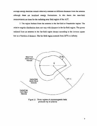
average energy densities remain relative ly constant at different distances from the anten na

although there are local ized energy fluctuatio ns. In this thesis the near-field

measure ments are done for the radiati ng near-field region of the AlIT .

3. The region farthest from the antenna is the far-fiel d or Fraunho fe r region . The

relat ive angu lar distribution does not vuy with distance in the far-field region . The powe r

radiated from an antenna in the far-fiel d region decays according to the inverse square

law as a functio n of distance . Th e far-field region extends from mIn.. to infinity.

........REACTIVE ,/

NEAR-FIEL0 -...LREGION t >

\-,, :::~~:'~L~ ..,------.....

RA~~::::- --:::~O_~ _FAR-FIELO

REGION

20' f A.

Figure 2.1 Three regionsof electromagnetic fieldsproduCl d by an antenna

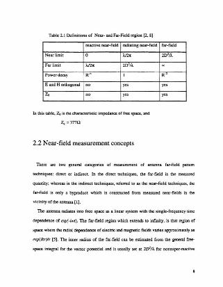
Tab le 2.1 Definitions of Near- and Far-Field region {2. 8]

reacti ve near-field r.tdiating near-field far-field

Near limit 0 m. 20 1n.

Far limit m. 20 ' ''- -Power decay R

O

' I RO

E and H orthogonal no yes yes

Z. no yes yes

In this table. Zois the characteristic impedance of freespace. and

z"mn

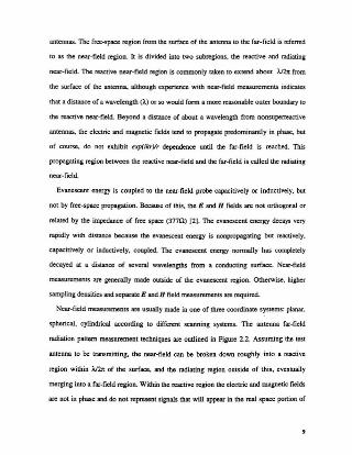
202 Near -field measurement concepts

There are two general catego ries of measurement of antenna far-field pattern

techniques: direct or indirect, In the direct techniques. the far-field is the measured.

quantity; whereas in the indirect techn iques., referred to as the near-field techn iques, the

far-field is only a byproduct which is constructed from measured near-fields in the

vicinity of the antenna (1].

The antenna radiates into free space as a linear system with the single-frequency time

dependence of ap(-iwr). The far -field region which extends to infinity. is that region of

space where the radial depend ence of electric and magnetic fields varies approximately as

ap(ikrYr [5]. The inner radius of the far-field can be estimated from the general free­

space integral for the vector potential and is usually set at urn. for nonsuper -reactive

antennas. The tree-space region from the surface of the antenna to the far-field is referred

to as me near-field region. It is divided into two subregions. the reactive and radiating

near-field. The reactive near-field region is commonly taken to ex tend about "AJa. from

the surface of the antenna. aJthough experience with near-field measurements indicates

that a distance of a wavelength ().,)or so would form a more reasonable outer boundaryto

the reactive ncar-field. Beyond a distance of about a wavelength from nonsupcrreactive

antennas. me electric and magnetic fields tend to propagate predominantly in phase, but

of course. do not exhibit exp(ikr )/r dependence until the far-field is reached. This

propagating region between the reactive near-field and the far-field is called the radiating

near-field.

Evanescent energy is coup led to me near-field probe capacitively or inductively, but

not by free-space propagation. Because of this, the E and H fields are not orthogonal or

related by the impedance of tree space (3nO) [2]. The evanescent energy decays very

rapidly with distance because the evanescent energy is nonpropagating but reactively.

capacitively or inductive ly, coupled. lbc evanescent energy normally has completely

decayed at a distance of several wavelengths from a conducting surface . Ncar-field

measurements are generally made outside of the evanescent region. Otherwise , higher

sampling densities and separate E and H field measurements arc required.

Near-field measurements are usually madein one of three coordinate systems: planar.

spherical, cylindrical according to different scanning systems. The antenna far-field

radiation pattern measurement techniques arc outlined in Figure 2.2. Assuming the test

antenna to be transmitting, the ncar-field can be broken down TOughly into a reactive

region within in« of the surface, and the radiating region outside of th is, eventua lly

merging into a far-field region. Within the reactive region the electric and magnetic fields

are not in phase and do not represent signals that will appearin the real space portion of

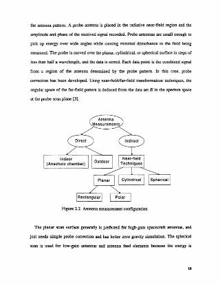
the antenna pattern . A probe antenna is placed in the radiative near- field region and the

amplitude and phase of the received signal recorded. Probeantennas are small enough to

pick up ene rgy over wide angles while causing minimal disturbance to the field being

measured. The probe is moved over the planar. cylindrical . or spherical surface in steps of

less than half a wavelength. and the data is stored, Each data point is the co mbined.signal

from a region of the antenna determined by the probe pattern . In this case. probe

correctio n has been developed. Using near-ficldlfar -field transfonnation techniques. the

angular space of the far-field panem is deduced from the data set E in the aperture space

at the probe scan plane (3).

Figure 2.2 Antenna measurement configuration

The planar scan surface generally is preferred for high-gain spacecraft antennas, and

just needs simple probe correctio n and has better zero gravity simulation. The spherical

scan is used for low-gain antennas and antenna feed clements because the energy is

10

captured at large angles from the AUf bores ight axis. Cylindrical surfaces are often used

with television broadcas t an tennas and certain spacecraft 1T&C omni antennas [2J.

2.3 Advantage of near-field measurement

When direct anten na measurem ent is performed outdoors. it may be affected by

weather conditions. multipath. erc.: when it is performed indoors. it needs to be measured

inside an expensive big size anecho ic cham ber. Becauseof this. near-field measurement

techniques are widely used today. Near-field techniques a) can give absolute

measurements including mismatch correctio ns. b) need not invo lve approx imations (in

the extrapo lation methods ) other than truncat ion of the infinite set of exact solutions used

in expressing the field. and c) apply [0 nonli near transmitting transduce rs and

nenreciprccal uansd ucers (foc example. arrays with ferrite phaseshifters or isolators).

whether transmitting. receiving, or scattering [12).

Additional ly. from the techn ical point of view . someof the advantages of near-field

measurement techniques over direct far-field pattern measurements include

(I) Near-field measurements are time and cost effective. and the accuracy of the

computed patterns is companble to that for the far·field range .

(2) The near-fie ld range provides a controlled environmen t and al l-weath er

capability.

(3 ) For large antenna systems. far-field range size limitatio ns. transporta tion and

mounting proble ms. and the require ment for large-scale posluoners are

eliminated.

II

The main advantage of near-field over direct far-field pattern measurements is cost. It

is much cheaper to build a scanner lhan building an anechoic chamber on acquired land

for antenna measurements .

2.4 Near-field antenna measure ment criteria

2.4.1 Grid spac ing criteria

The objectives of these sections are to establish a sample spacing criterion for near­

field measurements made on a plane surface near the antenna under tes t (Arm. and to

develop a near-field data minimization technique for reducing the computational effort

required to calculate a given portion of the far-field radiation parrern [13. 14].

When the probe is operating on a polar-planar scanning plane. Ute probe increment

between rings is usually taken at approximate ly 0.5 wavelength [I ]. It follows from Ute

two-dimensional Nyquist sampling theorem that, for the wavenumber limited spectrum.

the electric field can be reconstructed for all points on the plane z=O from a knowledge of

its values at the rectangular lattice of points separated by the grid spacing of an upper

limit of )./2 [14}.

2.4.2 Distance criteri a

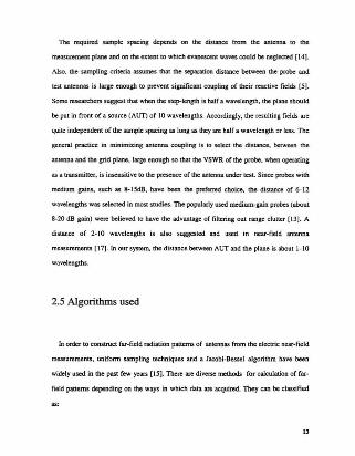
The required sample spacing depends on the distance from the antenna to the

measurement plane and on the extent (0 which evanescent waves could be neglected [14].

Also. the sampl ing criteria assumes that the separation distance betwee n the probe and

test antennas is large enough to prevent significant coupling of their reactive fields [5].

Some researchers suggest that when the step-length is half a wavelength . the plane should

be put in front of a source (AlII) of to wavelengths. Accordingly, the resulting fields are

quite independent of the sample spacing as long as they are half a wavelength or less. The

general practice in minimizing antenna coupling is to select the distance, between the

antenna and the grid plane. large enough so that the VSWR of the probe . when operating

as a transmitte r. is insensitive to the presence of the antenna under test. Since probes with

medium gains. such as 8-15dB, have been the preferred choice, the distance of 6-12

wavelengths was selected in most studies. lbe popularly wed medium-gain probes (abou t

8-20 dB gain) were believed to have the advantage of filtering out range clutter [13). A

distance of 2-10 wavelengths is also suggested and used in near-field antenna

measurements [I7 J. In our system, the distance between AUT and the plane is about 1-10

wavelengths .

2.5 Algorithms used

In order to construct far-fiejd radiation patterns of antennas from the electric near-field

measurements. unifonn sampling techniques and a Jacobi-Bessel algorithm have been

widely used in the past few years [IS]. There are diverse methods for calculation of far­

field patterns depending on the ways in which data are acquired. They can beclassified

IJ

(1) the uniform sampling in a rectangular coordinate system:

(2) the uniform or pseudo-u nifonn sampling in a polar coo rdinate system;

(3) the non-u niform sampling in a rectangular or polar coordinate system.

A Jacobi-Besse l algorithm has been used to calculate the far-field patterns in all the

above classes of measurements [IS1. Recently an FFT algorithm has been propose d

instead of the Iacobi-Bessel algorithm . Compared with the Jaco bi-Bessel algorithm . the

FFr a1goritlun consi derably reduces the time of calculation (I . IS] .

In near-field meas urement. the probe moves in two orthogonal linear directions. The

results are distributed in a rectangular coordinate system and the unifonn sampling

technique and FFT algorith m can be applied.

Far-field patterns may be calculated by using the FFr . given a set of near-field data

which have values on a rectangular coordinate system. J[ can be shown by application of

me Lorentz reciprocal theorem that the ourpcr voltage of the near-field measureme nt

probe is proporti onal to the antenna e lectric and magnetic fields Eo. and 11.- It can also be

shown that the relation between the motion of the probe in the measureme nt plane and the

antenna is a convolutio nal expression of the probe fields and the antenna fields E. and H.

(2). For polar scanning, the four-point Lagrange interpolation algorithm was first used in

orde r to use FFr to gel far-field patterns [16].

2.6 Validatio n

Validating the accuracy of any antenna measurement facility is difficult as there exists

no standard antenna with an associated standard antenna pattern which can be measured

to verify petformance and assess accuracy . The rwc tangen tial field components of a

I.

planar. cylindrical. or spherical surface enclosi ng the AlIT and separated from the

antenna by • distance of 2· 10 wavelengths are meas ured in amplitude and phase at

preselected sampling points over a prescribed portion of the enclosing surface in near­

field measurement systems. The accuracy of a far-fie ld pattern depends on the near-fie ld

measurement and the related measurement error through a modal transform (17].

The near-fie ld measurement and associated measuremen t error through a modal

transform determines the accuracyof the far- field pattern. Thus. approximate correction

factors are needed in order to account for the finite size and near-field distance: of the

measurement probe [5. 18]. 'The majorcompone nts of a near-field measureme nt system

which affect measurement accuracy can include hardware and software parts ; they are :

( I) finite sc:anarea

(2) distance:between the probe plane and the AlIT

(3) receiver nonlinearities in measuring the near-field amplitude

(4) someti mes multiple reflection

(5) the chamber, the computer and associated software [5, 17].

(7 ) the near electric field pattern of the probe

(8) reflection from scanner suppo n

The position drive system most commonly used is a de variable-speed electric motor

coupled to the moving members by a chain or lead screw. Desirablecharacteristics of the

drive system are smooth operation and constan t velocity with minimum vibration over a

wide velocity range [4].

It is recomm ended that the amplitude and phase indications of the receive r are

measured over a time interval of 8 h. The measurements begin after a 24-h warm-up of

both the receive r and the RF source. Theamplitude and phase measurements are repeated

"

at +3°C and ·3°C from the nominal tempe rature value (17]. In our system. the

measurements begin after about l-h warm-up.

Several criteria were considered in the developmen t of the: procedure to be used in

measuri ng the antenna far-field radiation pattern. These included repeatability of pattern

data. repeatability of system tes t power levels. accuracy of measurement, capability of

monitoring the:signal levels continuous ly. and dynamic range to make gain measurements

between two antennas of significantly different gains (I] .

Several aspects of the measurement technique must be cons idered..Both receiver and

amplifier gain (which are independently adjustable ) must remain constant during the test,

which may last as long as several days. In order to relate the reference levels of a

particular configuratio n to the antenna's radiated power. the receiver and computer

voltage levels are recorded while the probe is positio ned at one spot on the near-field of

the antenna. This spot is generally chose n to be approximately the:point of highest power.

and is referred to as the "boe spot". In order to obtai n the most dynamic range of the

receiver/computer . the probe is placed at this location and the receiver amplitude gain is

set below saturation . still in its linear region (II .

2.7 Planar scanning of near-field measureme nt

The development of near-field antenna measureme nt techniques can be divided into

four periods: the early experimental period with no probe correction (1950-1960). the

period of the first probe-co rrected theories (196 1-1975), the period in which the first

theories were put into practice (1965-1975). and the period of technology transfer ( [97 5­

1984) in wbkh 35 or more near·field scanners were built lhroughout the world [5. 19].

..

Modem planar scanning techniques in near-field measurement of antennas and scatters

are based on the plane-wave spectrum (PWS)_Planar scanning is IT'I()['C frequently used in

near-field measurements than cylindrical and spherical scanning because most directive

antennas have. on or near the antenna. an "aperture distribution- or "aperture

illumination- of finite extent slightly larger than the projected area of the antenna (13)­

Aperture antennas are most commo n at microwave rrequeocies, and they may take the

fonn of a waveguide or a hom whose aperture may be square, rectangular. circular.

elliptical. or any other configuratio n (20). For high-gain antennas. the planar

configuration is used most frequently [1).

2.7.1 Near-field sampling

In the planar near-field measurement technique. data are acquired on a plane which is

finite in extent but which intercepts the major portion of the radiating field. These data

are then used to calculale the far-field quantities of the antenna under test. The calculation

or the various quantities depends on the manner in which the data are acquired. Two

different near-field sampling coordinate systems ~ used to complete the planar near­

field measurements. One is measured in a rectangular coordinate system, and the other

one is in a polar coordinate system. General ly, three kinds of sampling in planar near­

field measurements are applied:

( I) the uniform sampling in a rectangular coordinate system;

(2) the uniform or pseudo-un ifonn sampling in a polar coordinate system;

(3) the non-uniform sampling in a rectangular or polar coordinate system.

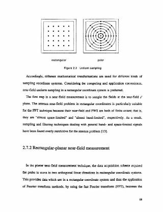
Figure 2.3 shows uniform sampling in a rectangular or a polar coordinate system.

11

rl cll ngu[lt pOl.,

Figute 2.3 Unilorm sampling

Accordi ngly, different mathematical transformations are used for different kinds of

sampling coordinate systems . Consideri ng the computing and application convenience,

near-field uniform sampling in a rectangular coordina te system is preferred .

The first step in a near-field measurement is to sample the fields at the near-field s:

plane. The antenna near-fie ld proble m in rectangular coordinate s is particular ly suitable

for the FFT tccbnique beca use their ncar-field and PWS are both of finite extent; that is.

they are -almost space-limi ted - and -almost band-limited", respecti vely. As a result.

sampling and filtering techniques dealing with general band - and space-limited signals

have been found overly restrictive for the antenna problem (13 ).

2.7.2 Rectangular-planar near-field measurement

In the planar ncar-field measurement technique. the data acquisition scheme required

the probe to move in two onh ogonal lineardirections in rectangular coordinate systems.

This provides data which are in a rectangular coordinate system and thus the application

of Fourier transform methods . by using the fast Fourier trans form (fFJ). becomes the

(.

obvious data reduction techni que (16]. Near-fiel d data are acquired on a plane which is

finite in elttem but which interceptS the major portion of the ndiation field. The Ier-fiejd

pattern is calcul ated from the mcasu.rcd near-field, When it is assumed that multip le

interactions between the probe and the test antenna are negligibl e, prcbe -coeected planar

near-field formu las can be used [ 18).

2.8 Limitations

I. Planar, cylindrical, and sph erical ncar-fiel d scanning can be formu lated 10include all

the multiple interactions betwee n the probe and test antenna [5].

2. Another limitation (besi des me neglect of multiple reflecti ons) within the basic theory

of planar ncar-field scanning limits the appli cation of planar scanning to directiv e

antennas [SJ.

3. Because of the size of the near-fie ld measurement scanner, the far-field antenna

radiation pattern we get from near-field meas urement cannot be ~360" or -180"- 180" as

the horizontal radiatio n pattern we meas ured by direct antenna measurement inside the

anechoic chamber .

I'

Chapter 3

Planar Near-Field Antenna Measurement

System

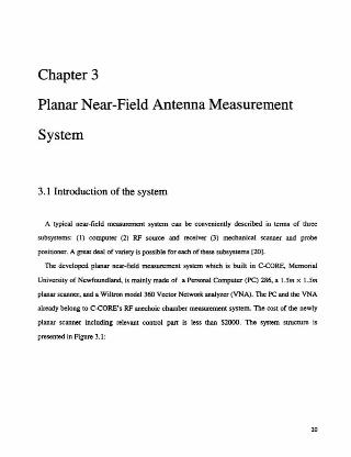
3.1 Introduction of the system

A typical near-fie ld measurement system can be conveniently describe d in terms of three

subsystems: (I) compute r (2) RF source and receiver (3) mechanic al scanner and probe

positioner. A great deal of varietyis possible for each of these subsystems [201-

The developed planar near-field measurement system which is built in C..cORE, Memori al

University of Newfoundland. is mainly made of a Personal Computer (PC) 286. a 1.5m )( 1.5111

planar scanner, and a Wil tron model 360 Vector Network analyzer (VN A). The PC and the VNA

already belong to C-CORE ' s RF anechoic chamber measurement syste m. The cost of the newly

planar scanner including relevant control pan is less than $2000 . The system structure is

presented in Figure 3.1:

20

PC

----------------------------------------1: Scanning: system__________ ____ ___________________________________________r

Figure 3.1 Near-field antenna measurement system

~ - --- - - - - ---,, ,, ,, ,, ,

j ~..

The probe on the planar scanner is driven by the dual motor contro ller. and moves in horizontal

and verticaJ direc tions. At certain position s, the probe will measure the magnitude and phase of

the near electric field radiated by the AUT which is kept at a certain distan ce from the scanning

plane, and shows on the VNA. After several measurements, the VNA will pass these data

magnitude and phase to PC storage for further proce ssing ..

3.2 Management component--PC

Because of the large amounts of datainvolved. computer control of lite measurement system is

essential. Th e PC in the near-field antenna measurement system perfonns the man agem ent duty,

21

controls the motion or the probe. collection or the da1a fro m VNA, and also the man agement of

the communication between VNA and PC. The management package is written in Quicltbasic

embedded Assembly languages . The management is perfonned in real tirne as shown in Figure

3.2.

Figure 3.2 PC management flowchart

3.3 Measuring equipment -- Vector Network Analyzer

A two-pan. Wiltron model 360 VNA, already part of C-eORE's RF anechoic chamber

measure ment system, is used in the near-field antenna measurem ent system to measure the

radiatio n pattern of AUf. It is made of a front panel. a scree n, a generator. and a sou rce, has a

frequency range of 40MHz - 4OGHt. and frequency reso lution of IOOKEz.

22

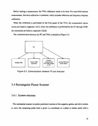
Before starting a measureme nt. the VNA calibratio n needs to be done. For near-field antenna

measureme nt. full-term calibration is preferred. which includes reflection and frequency response

cal ibratio n.

When the calibration is perform ed on the front panel of the VNA, the measurement option

menus are listed in Appendix I [2 t ]; when the calibration is performed by the PC through GPW,

the commands are listed in Appendix n (22).

"Thecomm unication between the PC andVNA is detailed in Figure 3.3.

Figure 3.3 Communication between PC and Analyzer

3.4 Rectangular Planar Scanner

3.4.1 System structure

The mechanical scanner (or probeposi tioner) consists of the supports, guides, and drive motors

to move the measuring probe from a given x-y coordi nate in a plane to certain point until a

23

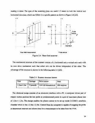
readi ng is taken. The span of lhe scanning plane can reach 1.5 meters in both the vertical and

horizontal direct ions which can fo llow in a specific patte rn as shown in Figure 3.4 [23].

----,Xi.Yj _ _

, I! !

.,

I

jII

iL

i'ii

I , ProblT ' ~ 1II0Iio ll

Nl a r·fieldm ll$Urlm e lll Probe mOlioll

Figure 3.4 Near·field scanner

The mechanical saucrure of the scan ner consists of a horizontal and a vertical axis each with

its own drive mechanism such that ei ther axis can be driven independent of the othe r. The

advanrage of the structure is shown in the fo llowing table 3. ( [23]:

Table 3 .1 Scanne r structure factors

The electrical design consi sts o f an electronic interface with a PC. A comp ute r dri ven pair of

stepper motors position the test pro be at predetermin ed po ints in a grid of maximum planar size

of 1.5m X 105m. This design enab les [he planar scanner to be set up inside C-eORE 's anechoic

cham ber which is 4m x 205m x 2.5m. Contro l fromtheco mputer is capable of stoppi ng the probe

at determined intervals and allow s time for a measure ment to be taken from the VNA.

"

Accord ing to the design. as the motors arc incremented. the number of steps reeved arc wed to

calc ulate a vertical or horizontal linear displaceme nt.

D ispfacement(meru sJ=munber ofSUP$ x 7.5degrees! 20rurnslin chx 0.0254

Using this equation. one can calculate relative motor running turns to de termi ne the probe

posit ion.

3.4 .2 A· BUS Adapter and ST· 143 dual step motor contro ller

An AR- l33 card. A-BUS adapter which can be used for the ffiM PClXT/AT and all

co mpatibles . is co nnected with the step mot or co ntro ller. A-B US adapter whic h can be inserted

into the PC. converts the signals avai lab le on the PC to the universal A·BUS standard . This

insures tha t any current or future A-B US card will work with the system. It has four essential

des ign goals : (1) Reliability: quali ty co mponents. uncompromised desi gn: (2) Low cos t: savings

311: ach ieved by clear design and effic ient bus structure ; (3) Simplicity and Expandability: (4)

Univ ersal ity .

The co mplete A·BUS system that we used consists of a driv er circuit, AR· 133. which is an A·

BUS Adapter and located on the It)·b it bus inte rnal to the com puter. The schematic of AR-t33.

the A-BUS adapter , is shown in Figure 3.5.

2l

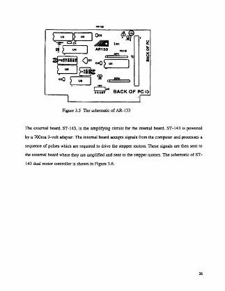
Figure3.5 The schematic of AR·1 33

The external board. ST-143 . is the amp lifying circuit for the internal board . ST·1 43 is powered

by a 700m a 9-vo lt adapter . The internal board acce pts signals from the co mputer and processes a

sequence of pulses which are required to drive the stepper motors . These signals are then sent to

theexternal board where the y are amp lified and sent to the stepper motors . Tbe schematic of ST­

143 dual motor controller is shown in Figure 3.6.

26

Figure 3.6 Schematic of dual motorcontroller

3.5 System Communication

In order 10 record the near-field antenna measurement data picked up by the probe.

communication is built between the dual stepper malar controller. the PC. and the VNA.

Different communication components are used for different proposes. The basic system

communication structure is shown in Figure 3.7.

27

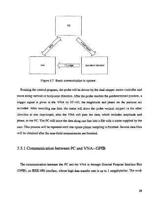
Figure 3.7 Bas ic communication in system

Running me control program.me probe willbedriven by me dual stepper moto r controller and

move along verncal or horizontal direct ion. After the probe reaches the predetenni ned position. a

trigger signal is given to the VN A by ST- 143. the magn itude and phase on the position are

recorded. After recordi ng one line, the motor will drive the probe vertical suppon on the other

direction at one step-length, also the VNA will pass the data, which includes amplitude and

phase. to the PC. The PC will sto re the data along one line into a file with a name supplied by the

user. Th is processwill berepeated un til one square planar sampli ng is finished. Several data files

will beobtained after the near-fie ld measurements are finished.

3.5.1 Commu nication between PC and VNA--GP ffi

The co mmunication between the PC and the VNA is through General Purpo se Interface Bus

(GPm ). an 1EEE4 88 interface, whose high datatransfer rate is up to I megabyt~sec. The work

28

is done by a program written in Quickbas ic embedded Assembly. The high data transfer rate

satisfies the real time contro l demand. The flowchan is shown in Figure 3.8.

Figure 3.8 Comm unica tion be tween PC an d VNA

The re are three VNA chan modes available: a) Polar Format; b) Log Magni tude and Phase; c )

both Polar and Rectangular . In planar near-field measureme nts. we use magnitude and phase.

During the measurement , the VNA is not permitted to input data from the front paneluntil 'clear '

is operated first, After finishing ncar-field measuremen ts, the YNA will be returned to local

control. 'Theuser can input data and operate on the fronc panel of the VNA.

29

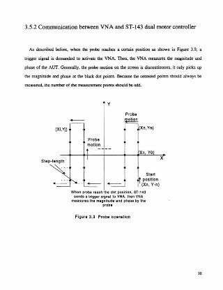
3.5.2 Communication between VNA and ST-143 dual motorcontroUer

As described betcee, when the probe readies a cenai n position as shown in Figure 3.9, a

trigger signal is demanded to activate lhe VNA Then , the VNA measures the magnitude and

phase of the AlIT . Generally, the probe motion on the screen is discontinuous. it only picks up

the magni tude and phase at the black doc: points. Becauselhe centered points should always be

measured. the number of the measurement points should be odd.

y

(Xi.Yj)

Probe

~

Xn,Yn)

Probemotio n

Xn. YO

Startt posili on

(Xn. Y·n)

x

Whl n probe r••ch Ih, uct posit ion, ST· 143Sin d, I trill ger signal to VNA. then VNA

m...urU lh, malln il ude andphasa by l haprobe

Figure 3.9 Probe operation

30

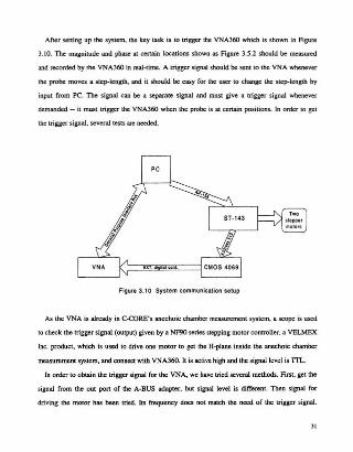
After seu ing up lite system. the key task is to trigge r lhe VNA360 which is sho wn in Figure

3.10. The magnitu de and phase at certain locati ons shown as Figure 3.5.2 shou ld be measured

and recordedby the VNA360 in real-time. A trigge r signal should be sent to the VNA whenever

the probe moves a step-length , and it should be easy for the user to change the step-length by

input from PC. The signal can be a separate signal and must give a trigger signal wheneve r

demanded - it must trigger the VNA360 when the probe is at certain pos itions . In order to get

the trigger signal. several tests are needed.

Figur. 3.10 Syst em communication Ul up

As the VNA is already in C~ORE's anec hoic chamber measurement system, a scope is used

to check the trigger signal (output) given by a NF90 series stepping motor controller. a YELMEX

Inc. prod uct . which is used to drive one motor to get the H-plane inside the anechoic chamber

measurement system, and connect with VNA360 . It is active high and the signal level is Tn...

In order to obtain the trigger signal for the VNA, we have tried several methods . First, get the

signal from the out port of the A·B US adapt er. but signal level is different. Then signal for

driving the motor has bee n tried. Its frequency docs nol match the needof the trigger signal.

31

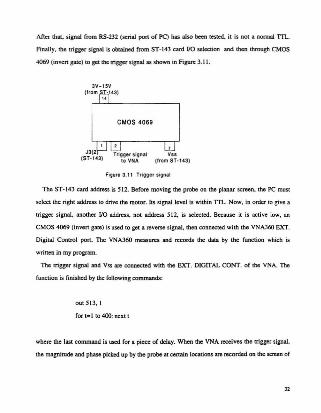
After that. signal from RS·232 (serial port of PC) has also been tested, it is not a normal TIL

Finally. the trigger signal is obtained from ST· 143 card ItO se lection and then through CMOS

4069 (inve rt gate) to get the nigger signal as shown in Figu re 3. 11.

Figure 3.11 Trigge r signal

The ST- 143 card address is S12. Before movi ng the probe on the planar scree n. the PC must

selec t the right address to drive the motor . Its signal level is within TIl... Now. in order to give a

trigge r signal . another ItO address. not address 512, is selected. Because it is active low, an

CMOS 4069 (invert gate ) is used to get a reverse signal. then connected with the VNA360 EXT.

Digital Conuel pan. The VNA360 measures and records the data by the function which is

writte n in my program.

The trigge r signal and Vss are connected with the EXT. mOrrAL CONT. of the VNA. The

functio n is finis hed by the following commands:

outSl 3. I

for te l to 400: next t

where the last command is used for a piece of delay. Whe n the VNA receives the trigger signal.

the magnitude and phase picked up by the probe at certai n locations are reco rded on the screen of

32

the VNA. The motion is repealed until one vertical line measurement has been finished. Then the

magnitude and phase meas ured are passed to the PC and saved as a data file.

3.5.3 Communication between PC and Stepper motor controller

As desc ribed before . the PC controls the functio n of ST-143 . a stepper motor controller.

through AR- 133. an A·B US adapter.

In the system. the A-BUS adap ter . AR- 133. is plugged into the computer. and connected with

the A-BUS card. ST-143 . Th e PC controls the motion of the stepper moto r controller by software

program . The program for driving the probe and giving the trigge r signal to VNA is written in

Quick bas ic langu age. and is stored in the PC. The user just needs to interface with the PC. The

flowchart of PC management of the motion of the dual stepper moto r contro ller is shown in

Figu re 3. 12.

33

Figure 3.12 PC managemenl ol the step permolorco nlroller

After the communications between the PC and the VNA. the PC and the stepper motor

controller. and the VNA and the stepper motor controller have been set up. the communication in

the whole near-field measurement system is shown in Figure3. 13.

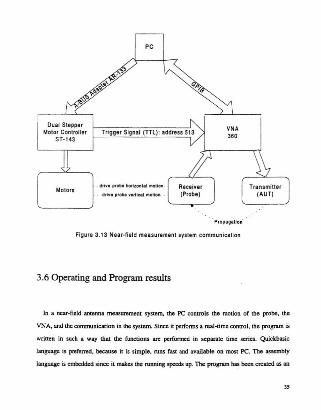
. Propagatio n

Figure 3.13 Near-field measu rement system communication

3.6 Operating and Program results

In a near-field antenna measurement system, the PC controls the motion of me probe. me

VNA. and me communication in me system. Since it performsa real-time control, me program is

written in such a way that me functions are performed in separate time series. Quickbasic

language is preferred, because it is simple. runs fasE and available on mcsr PC. The assembly

language is embedded since it makes me running speeds up. The program bas been created as an

as

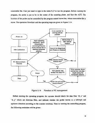
executab le file. User just need to type in the name N_F to ron the program.. Before running the

program. me probe is put to be in the center of the: scanning plane. and face the AUf. The

location of me probe can be co ntrolled by the program named move.bas. whose executable file is

move. Theoperation flowchart and the ope rating steps are given in Figure 3.14.

Figure 3.14 Flowchart of PC ma na ge me nt

Before running the operating program. me operator should check the data files ~ di_x· and

~di-y~ which are direction files . and indicate whether the probe mo ves in a lefVright and

up/down directio n accordi ng to the scanner condition. Then in running the controlling program.

me foUowing reminders will be given :

36

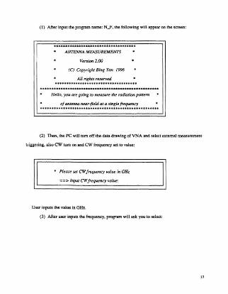
( I) After input lhc:progr.un name : N_F, the following will appearon the screen :

ANTENNA MEASUREMENTS

Version 2.00

(C) Copyright Bing Yan /996

All rights reserved....................................Hello , YO" are going to measllTe the radiation patte rn

ofan/mna near-fi eld at asingit' freq"t'ncy....................................................

(2) 'Then, lhe PC will tum off the datadrawing of VNA and select external measurement

triggering, also CW tum on and CW frequency set to valuc:

I• Please set CWfrequency value in GHz

==> [rIp"t CWfrequency valUt'!: I

User inputs the value in GHz..

(3) After user inputs thefrequency, programwill ask you to se lect:

31

This part ofprogram is used to s~l~ct

• the cluut mod~ di.splay~don 1M{ro nt pc1IfLl •

For NIF measuu~lIt, W~ Choos~ 2..........................................• J. Display in Polar Fomuu

• 2. Display ill Log Map.ituth and Phas~

• 3. Display in both Polar and Rect4Jlguiar

==> Pl~as~ input t , 2. and 3?

In near -fiel d antenna measurement, we choose 2. If user choose other data not I. 2, 3, then

~ no choice! ~

will appear on the screen .

(4) The PC will set the following information to VNA now

a) Set the display start from 0 and stop at 360 degree

b) Tum on data drawing

c) Active channel info rmatio n

This pan of tlte program is u.s~d to

• drive theprob~ acco rding to tM wav~l~"gth •..........................................==> Please input the maximum displac~me"t in nut~r

If lhe displacement inputted> 1.5m, it will ask the user to inpu t agai n; otherwise it appears

38

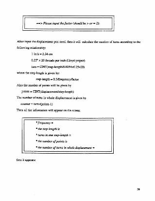
==> Please input the fa ctor (should be > or =2):

After input the displacement you need, then it will calculate the number of turns according to the

following relationship:

I inch = 2.54 cm

0.2r x 20 threads per inch (Uoyd project )

tum ::Cll'IT(step-lengthlO.0254xO.25x20)

where the step-length is given by:

step-length =0.3/frequencylfaetor

Also the number of points will begiven by

points « CINT(displacementistep-length )

The number of turns in whole displacement is given by

counter e tumx tpoints -I }

Then all the information will appear on the screen:

• frequency ::

• the step-lengtn is

• rums in one srep-length =

• rhe number of po ints is

• the number of tums in whole displacement =

then it appears :

"

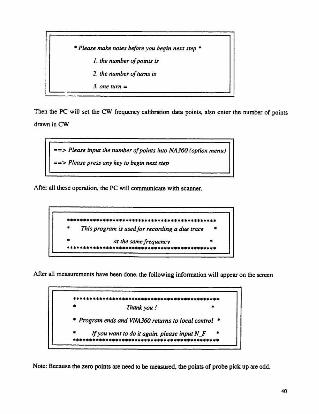
• Please make notes hefor e you begin next step·

I . the number ofpoints is

2. the numbe r of tu17U is

J . one tum =- ""

Then the PC will set the CW frequency calibratio n data points. also enter the number of points

drawn in CW

==> Please input the number of points into NA360(option menu )

==> Please press any Jcey to begin nut step

After all these operation. the PC will communicate with scan ner.

This program is usedfor recordi ng a due trace

at the same treauencv........"'..............•..••...•..............After all measure ments have been done, the followi ng information will appear on the screen

Thankyou!

• Program ends and VNAJlSOreturns to local control '"

Note: Because the zero poi nts are need to bemeasured. the points of probe pick.up are odd.

Chapter 4

Near-F ield to Far-Field Transformation

Since an antenna is • device for transforming a transmission guided wave into a wave radiated

in space. or vice versa, and the distribut ion of field strength about an antenna is a function of

both the distance from the antenna and the angular coordinates. the objective of this chapter is to

determi ne antenna radiation patte rns, and give the proper transfo rmation of the far-field radiatio n

patte rn.

4.1 Far-field determination from source distributions derived

from near-field measurements

Com plete electric E. and magnetic il fields within a given volume can beexpressed in terms

of the current densities of the sources within the volume and thevalues of the field itself over the

boundaries of the volume. If the volume of interest is defined to contain no sources and to be

bounded by a closed surface S and the sphere at Inflnuy , the E. and ii fields at a point P within

the volume are:

..

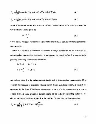
E~ = :iKI.[-iww(iix m il' +(iix E ) x VlY+ (n · E )V lfoda)

H~ =i;;J.[-iwU(iix E)." + (ii x H) x VVf+ (n · H)V ytda)

(4 .1)

(4.2)

where ;j is the unit vector nonnal to the surface. The function ", is the scalar portion of the

Gree n' s functio n and is given by

(4.3 )

where k is the freespace wavenumber (21t1A.) and r is the distance from a poi nt on the surface to a

field point [6}.

When it is desirable to determine the current or charge distrib ution on the surface of the

antenna rathe r than the field distri bution in an aperture , the closed surface S is assumed to be

perfectl y cond ucting andboun dary conditions

ii x E= O ;, x H= K

ij -E = & ;j ·H= Oe

(4.4)

are app lied. where K is the surf ace curren t density and P. is the surface charge density. If , in

additi on, the equation of continuity relating curren t densi [y and charge density is util ized. the

equations for theE and H fie lds can be expressed in terms of either curre nt density or charge

dens ity alone . In terms of surf ace CUlTCnt density on the perfectly conducting surface S, the

electric and magnetic fields at a point P in the volume of interest then can beexpressed as

(4.5)

(4 .6 )

Thus. in its fundamenlal formulation. the method of delemtin ing field partems from source

distributions involves the application of (4.1. 2) for aperture distributions or (4.5. 6) for current

distributions. In the first case. near-field measurements are made to determine the E and H field

distributions over a surface surrounding the antenna [6]. Except for very simple geometries.

(4. 1-2. 5-6) are extre mely difficult to apply without approximations. These approximations

usually relate [0 the ruru re of the fields or currents on the surface over which the integration is

perfonned.. The approximations that are necessary to permit evaluation of the surface integrals

usually fall into one of lhe following areas:

( I) Assuming negligible contribution of the fields or currents over some portion of the

surface:

(2) Assuming all radiation follows outward normalize to the surfacc;

(3) Assuming the electric and magnetic fields are linearly related as in a plane wave;

(4) Assuming small-angle approximations and thus limiting the angular region for

IlXaling the field point.

Approximations of this type should be disti nguished form the normal far-field approximations

that simplify computation but produce valid results at distances sufficiently far from the source to

satisfy far-field conditions.

.o

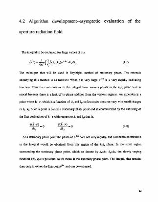
4.2 Algorithm developmenr-asymptotic evaluation of the

aperture radiation field

The integral to beevaluated for large values of r is

(4 .1)

The technique thal will be used is Rayleigh's method of stationary phase. The rationale

underlying this method is as follows: When r is very large e·p.r is a very rapidl y oscillating

function. Thus the contributions to lhe integral from various points in me k):, plane tend to

cance l because there is a lack of in-phase addition from me various regions. An exception is a

point where k . r , which is a functio n of k~ and k,. to fll'Storder does not vary with small changes

in k~. k" Such a point is called a statio nary phase point and is characterized by the vanishing of

the rust derivatives of k . r with respect to ka and k,; that is.,

a(k · f) = 0at ,

(4 .8 )

At a stationary phase point ihe phase of c·jkr does not vary rapidly, and a nonzero contribution

to the integral would be obtained from this region of the lzk, plane. In the small region

surrounding the stationary phase poi nt. which we denote by k~k" k,=k,• the slowly varying

functio n f(k... t ,) is put equal to its value at the stationary phase point . The integral that remains

then only involves the function e'~~ and can be evaluated.

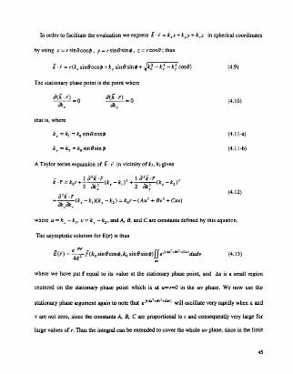
In orderto facilitate the evaluation we express i · f :: t , .r + k, Y +t,4 in spherical coordinares

by using .r= rsi n8cos " y = rs in8 sin " t = rcos8 ; thus

f · f = r(k . sin8 costll+k .• sin8sinq, + ~k; - k~ - k _~ cos8) (4.9)

The slalionary phase point is the point where

(4.10)

that is, where

(4.1 I-a)

(4.1 I-b)

A Taylor series expansion of f -r in vicinity of K" K2gives

(4. 12)

where u = k, -k l • V =k, -k1 , and A. B. and C are constants defined by this equation.

The asymptotic solution for E(r ) is thus

where we have put f equal to its value at the stationary phase point, and .:.\sis a small region

centered on the stationary phase point which is at u=v=Oin the uv phase. We now use the

stationary phase argument again (0 note that eJ I""· . ..·. c..., will oscillate very rapidly when u and

v are not zero , since the constants A. B, C are proportio nal to r and consequently very large for

large values of r , Thus the integral can beexlCnded to cover the whole uv plane. since in the limit

"

as r becomes infinite the contributions from u and II outs ide of 4s will caned from phase

interference. Hence we need to evaluate lhe follo wing express ion:

Because:

and put J'Au+ (Cv /2J'A) '" w to get forme integral the result

Next we use the known result

to evaluate the integrals over w and v. We then obtain

I '" 44/;: Cl '" 2ltj~COS8

upon using

Our final result is lIS)

(4.14)

(4. 15)

with

i ,(k , .k ,)' JJ l . (z.1)<" ··' ·' duly

'.Equation (4 .8) and (4.9) willbeused to gel the far-field radiation patterns.

4.3 FFT Algorithm used for far-field

(4 .16)

(4.17)

In a source-tree region in which near-fields are measured. the lime-harmo nic Maxwell

equations can be transformed into:

The far-zone radiation field computed from the aperture: electric field is given by [2S]

where the following fast Fourier transforms (fFI) are used:

(4. I9-a)

(4. 19-b )

"

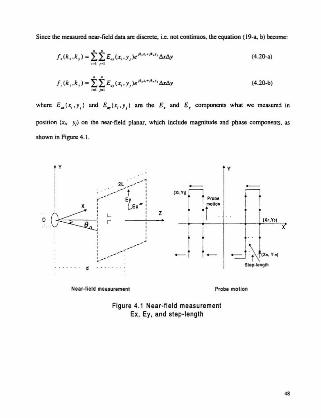
Since the measured near-field data are discrete, Le. not continuos. the equation ( 19-a, b) become:

I . (k • •k , )= ti:£_(X;.y,)e......•..·,,~y.~I ~I

I . (l,. k,) '" i:i:E... ( x•• y,)e...·..•... · -',~y,~I ,~ l

(4.20-a)

(4 .2<l-b)

position (x.. y, ) on the near-field planar. which include magnitude and phase compo nents. as

shown in Figure 4.1.

. y

....,i 1i i .,L.

.j~(X'.'"St. p4 .1Igl1l

Nn r·fit ldmtasutemtnl Probe molion

Figure 4.1 Near-field measurementEx. Ey. and step-length

..

.1.tand .dy are equal to step-length

tu "" l1y ""_4_ ifac ror?;1)facr or

(4.2 1-a)

(4.21-b)

(4 .22)

After submitting these definitio ns, we can get far-field radiati on panemsfrom equation (21-a &

2 1-b).

In fact. the network analyzer measures gain instead of E . Whe n we apply the FFf algorithm to

get far-field radiation patterns. we use the following equatio n in programming:

It is because of

p=.F.xR

and outside of the reacti ve (evanescen t) ncar-field region . the E and H fie lds an: re lated by the

characteristic impedance of free space (3770 ) [2}.

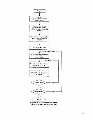
4.4 Algorithm application

After the near-field meas urement has been performed. the next step is to use the algorithm

described alone to calcul ate the far-fi eld radiation pattern. The following flowchan in Figure 4.2

descri bes the operation in detail.

"

V..

~NOVe.

~Fig ur e 4.2 F lo wchart of near­fialdlfar·field tra nsfo rmation

so

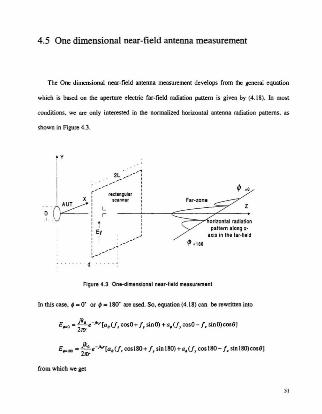
4.5 One dimensional near-field antenna measurement

The One dimensional near-field antenna measurement develops from the general equation

which is based on lhe aperture electric far-field rad iation pattern is given by (4.18). In most

conditions, we are only interes ted in the nonnalized horizontal antenna radialion patterns. as

shown in Figure4 .3.

r "_/ --1

~I r----:':,.", !:,

X I letnn"

~~ i ~ --...,...-- --.:=--- 7"'<---, ., I: Ey I

:, I _ _---- --.>

~ -» -

Figure 4.3 One-dimensional near-field measurement

In this case, , = O' or. =ISO' are used. So. equation(4.18) can be rewritteninto

£..0 =;~ 1!- ..... [a, (f~ cosO+ I , sinO)+12, (/ , c050 - r, sinO)cos8]

E..11O =;~ e -N(lJ,U.cos l80+ I , sin ISO) +rJ.U , cos ISO- f . sin ISO)cos8 ]

from which weget

"

(4 .23 -&)

(4 .23- b )

where

and we can get

It. I=It_I

1t.1 =1t••1

(4 .24 )

4.6 Probe-correction for planar near-field scanning

When near-field antenna measurements ee performed. the collected data are the received

power of a probe. which has a known near-field receiving radiation pattern, results from scanning

on a plane in front of the AUT. The assumes that the probe receives with ominidirectional

capability and that multiple interactions between the probe and the test antenna are negligible

[18] .

52

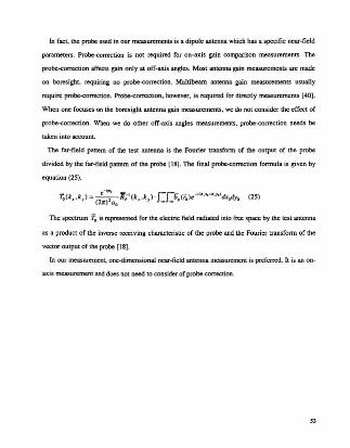
In fact. the probe used in our meas uremen ts is a dipole antenna which has a speci fic near-field

parame ters . Probe-correctio n is not requ ired for on-axis gain comparison measurements . The

probe-correction affects gain on ly at off-axis angles. Most antenna gain measureme nts are made

on boresight, requiring no probe-com:ction. Multibeam antenna gain measurements usually

requ ire prcoe-correcuc n. Prcce -eorrecuoe, however, is required for directly measuremc:nts (40 ).

When one focuse s on the OOresig ht antenna gain measurements, we: do not co nsider the effect of

probe-correction. When we do other off-ax is angles meas urements. probe-correc tion needs be

take n into account.

The far-field pattern of the test antenna is the Fourier transform of the output of the probe

divided by the far-field pattern of the probe (18]. The final prcee-ccrrecucn formula is given by

equat ion (25) .

The spectru m 10 is represented for the electric field radiated into me space by the test antenna

as a prod uct o f the inverse receivi ng characteristic of the probe and the Fourie r transfo nn of the

vector output of the probe [ 18J.

In our measuremen t, one-d imensional near-fie ld antenna measurement is preferred. It is an on­

axis measurement and does not needto consider of probe correction .

"

Chapter 5

Validation of the System

Several prelimi nary, one..<fimensional tests were performed to find the required near -fie ld

spacing and scan size. the best value of the prcce -entenna-separauon distance. and to find the

level of the leakage. and to reduce it. if necess ary. Comparisons with the far- field radiation

patterns obtained by direct measurement inside C-CORE 's RF anechoic chamber will determine

the success of the developed near·fie ldlfar-field measurement system.

5.1 Description of Antenna under test

In the tests. we use two different antennas as the AUf: one is an UC band microstrip antenna

which was designed and built following spec ifica tion set by the Canadian Space Agency (CSA)

for sate llite-based Synthetic Aperture iUdars (SAR 's) ; the odlcr is a hom antenna.

5.1.1 UC band microstrip antenna

The CSA specificalions for an U C band micros trip antenna requires operation in both the L

band at 1.275 GHz and in the C band at 5 .3 GHz. This antenna was designed. built and tested

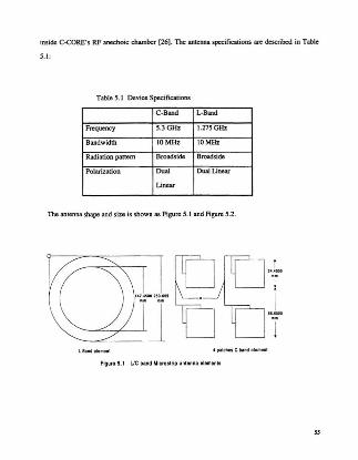
inside C-eORE's RF anech o ic chamber (26). Tbe antenna specific ations ere described in Tab le

5.1:

Table 5.1 Device Speciflcations

C-Band L-Band

Frequency 5.3GHz 1.21SGHz

Bandwidth 10 MHz 10 MHz

Radiation pattern Broadside Broadside

Polarization DwoI Duall.inear

Linear

The ante nna shape and size is show n as Figure 5.1 and Figure 5.2.

~¥6~.;~

14 U$IO ZS0.1$' 0 II....M_

L IlIld . l.lII.,,'

Figur.5.1 UCban d MicrOllrlp anl. nn. tl .mtnll

ss

Figure 5.2 UC microslrip antenna

5.1.2 Hom antenna

The hom antenna used here is a commerci al antenn a. lls structure is shown as Figure 5.3.

PM 7320X$IVERSLab Frequency: 9.35 GHz

~t".khOlm S " d," .

. . 1.S

•. ~ : _ ..••.. - . . . • ' . 5.1

:.:.. -. ~.

u. s~

Figure 5.3 Antenna under testhorn antenna

The operating frequenc y is 9.35 GHz.

5.2 Test sample spacing

The test-sample-spacing procedure was used to find the required near-field spacing. It

consisted of taking one-dimcnsional scans in x and y with very fine spacing (about 0.25),). First,

an FFT was performed on the full set of data, then using only every other point. then using every

third point. and so forth. Fro m this , we:could compare the far-field spectra from various spacings.

The smallest spacing was assumed adeq uat e:. When the spaci ng from the other FRs was so large

that the spectru m changed by more than the desired accuracy. a spaci ng equal 00or smaller than

the next smallest spacing was used .

From these onc-dimensional tests . we concluded that the spacing between near-field data

points should have been abou t O.5J.. for the L band and 0.24). for the C band for microstrip

antenna; and 0.5). for the hom antenna. in both • and y. where ). was changed according to

different band.

5.3 Test scan-length and distance

In princi ple, the planar near- field method assumes measurements on an infinite plane . Since

this is impossi ble. we had to determine the required scan size to obtain medes ired accuracy ove r

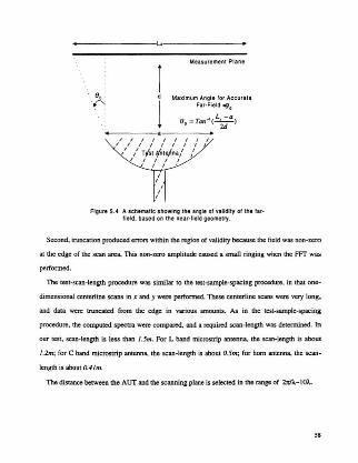
the angular regio n of interest, This scan -area truncation had two effects . Fim, jhe far-tield results

were valid only within the angular region 60 defined.by the AUf aperture and the scan area as

shown in Figure 5.4.

SI

_-- - - - Il>,- - ---_

Measurement Pla ne

8,«-. Maximum Angl8 lo r Accurat e

Far'F i 'la~o

90

= Tan-'( L~a )

Figure $.4 A schematic showing the angll of validity 01 the Iar­field. based on the near.l ield lll ometry.

Second. truncation produced errors within the region of validity because the field was non-zero

at the edge of the scan area. Th is non-zero amplitude caused a smaIl ringing when the FFT was

performed.

The test-sean-length procedure was similar to me rest-sample-spacing procedure. in thai one­

dimens ional centerline scans in z and J were performed. These centerline scans were very long ,

and data were trunea1ed from the edge in various amounts. As in the test-sample-spacing

procedure . the computed spectra were compared. and a required scan-length was detennined. In

our lest. scan-length is less than I.5m. For L band microstrip antenna. the scan-length is abou t

1.2m; for C band microstrip antenna, the scan-length is about O.5m; for hom antenna, the scan-

length is about O.4Im.

The distance between the AUT andthe scanning plane is selected in the rangeof 27C!J..-IOl..

"

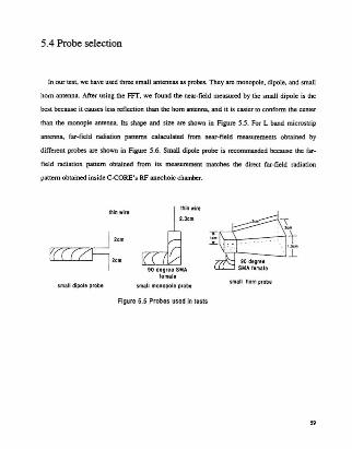
5.4 Probe selection

In our lest, we have used three smaIl ante nnas as probes. They arc monopole. di pole. and small

hom antenna After using the FFT. we found the near-field measu red by the small dipo le is the

best because it causes less reflection than the hom antenna. and it is eas ier to confonn the ce nter

than the monople antenna. Its shape and size arc shown in Figure 5.5 . fU L band micros trip

antenna. far- field radiation patterns calacuJaled from near-field meas urements obtained by

differe nt probesare shown in Figure 5 .6. Small dipole probe is recommanded because the far­

field radia tio n patte rn obtained from its measurement matc hes the direct far-field radiation

patte rn obtained inside C-e ORE ' s RF anechoi c chamber .

......"J"""'''Z.3c1ll

~2::mr.L..i...L.Ll'j 90 d.gr • • SMA

lemal,

small dipoll prob. small monopol. probe

Figure 5.5 Probes used in lests

~. ::.

:E __ : T---- . ·- I90 cl' grll

SMA r.mal,

sm, ll horn probl

ss

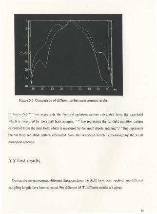
Figure 5,6 Compariso n of different probes measurement results

In Figure 5.6 '' ." line represents the far-field radiation pattern calculated from the near-field

which is measured by the small hom antenna; "." line represents the far-field radiation pattern

calculated from the near-field which is measured by the small dipole antenna;"}·" line represents

the far-field radiation pattern calculated from the near-field which is measured by the small

monopole antenna.

5.5 Test results

During the measurement s, different distances from the AlIT have been applied. and different

sampling length have been selected, For different AUT, different results are given,

60

5.4.1 Test results for U C band microstrip antenna

When we put the UC band microstrip AUT. the key characte ristics are given in Table 5.2:

Table 5.2 Near-field measurement characteristics (Microstrip antenna )

C·Band L-S'"

Operatingfiequency 5.79GHz 1.29 GHz

Probe shape & size 4cmdipole 4cmdipole

Distance between probe & AlIT{d) 13 cm JOcm

Number of discrete points 19x 19 9>< 9

Grid size O.466m 1.213m

eo 32.60 56.69"'

where eo is the largest angel from broadside direction with accurate results as shown in Figure

S.4 before. After ncar-field meas urement. we apply the FFi transfonnatio n to gel far-field

radiationpatterns. h is shown asFigure 5.7.

61

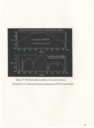
Figure 5.7 Far-field radiatio n patterns of microstrip antenna

(calculated by two-dimensi onal and one-dimensional NFIFF measurement )

62

5.5.2 Test results for hom antenna

Other antennas have been used as Al.Jf. such as the hom antenn a which has a ope ration

frequen cy of 9.35 GHz. Its charac teris tics are listed in Tab le 5.3:

Table S.3 Near -fie ld meas urement of hom antenna

Operatingfrequency 9.35GHz

Probe shape& size 4cm dipole

Distance between probe & AUT (d) n om

Numbe r of poin ts 29x:29

Grid size 0.41 m

e. 39.20

Figure 5.8 gives the far-field radiation patterns calculated by one-d imensional and two­

dimen sional near-field meas urements.

sa

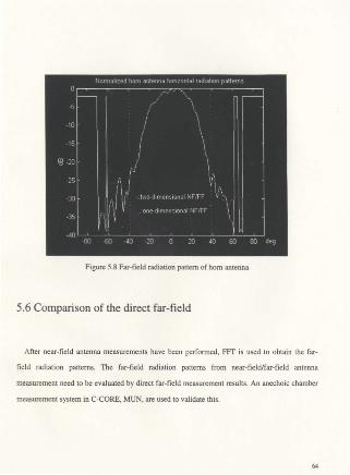
Figure 5.8 Far-field radiation pattern of hom antenna

5.6 Comparison of the direct far-field

After near-field antenna measurements have been performed. FFT is used to obtain the far­

field radiation patterns. The far-field radiation patterns from near-field/far-field antenna

measurement need to be evaluated by direct far-field measurement results. An anechoic chamber

measurement system in C-eORE. MUN. are used to validate this.

..

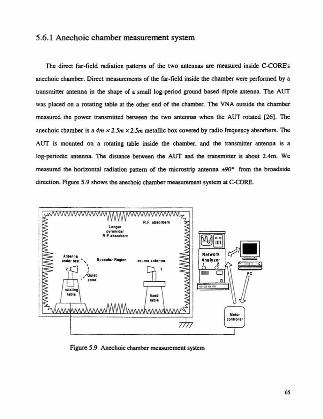
5.6.1 Anechoic chamber measurement system

The direct far -field radiation patterns of the two antennas are measured inside C-eORE's

anecho ic chamber. Direct measurements of the far-field inside the chamber were performed by a

transmitter antenna in the shape of a small log- period ground based dipole antenna. The AlIT

was placed on a rotati ng table at the other end of the chamber. The VNA outside the cham ber

measured the power transmitted between the two antennas when the AlIT rotated [261. The

anechoic chamber is a 4m x 205mx 205mmetallic box covered by radio frequency absorbe rs. The

AUf is mounted on a rotating table inside the chamber. and the transmitter antenna is a

log-periodic antenna. The distance between the AlTl" and the trans mitter is about 2.4m. We

measured the horizontal radiation pattern of the microstrip antenna~· from the broads ide

direction. Figure 5.9 shows the anechoic chamber measurement sys tem at C-CORE.

Figure 5.9 Anechoic chamber measureme nt system

"

The compu ter will drive the motor conuoller to rota1e the table and record the measurement

from the VNA. The VNA .....e used is a two-pott Wiluon product Model 360 whicb bas a

frequency range of 4OMBl · 40GBl and mquency resolution of looKHl . The motor controller is

the NF90 stepping motor controller which. is produced by Velmex Inc.. The communication

between the PC and the motor controlle r is performed by RS-232 . Quickbasic embedded

assembly language is used in programming.

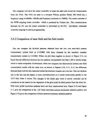
5.6.2 Compariso n of near-field and far-field results

One can compare the far-field pattern s obtained from the low cost near -field antenna

measureme nt system built in C·CORE with those obtained by the anechoic chamber

measuremen t system in C-eORE. When we plot them together as shown in Figure 5.10. we

found that the di ffere nce between the tw o patterns was generally less than 5 dB in validity range.

which is rathe r acceptable. Furthennore . when one compares one-dimensional antenna near-field

measurement results with the other two . as shown in Fi~ 5.10 . 5.11. 5.12 , the di fference

betwee n them and the data measured inside the anechoic chamber areeven less . One can attribute

this to the fact that the dipole is more omnidirec tional as it travels horizontall y paral lel to the

AUT than when it moves. The changes in the dipole gain when it travels vertical ly can be

considered as the reason for the departure of the grid mode l fer-fie ld pattern from the direct far­

field since probe correcti on methods have not been implemented here. Figure 5.10 and Figure

5.11 give the comparison of the UC band microstrip antenna horizontal radiation pattern ; and

Figure 5.12 gives the comparison of horn antenna horizontal radiation patterns .

se

FigureS.I0 Comparison of L bandmicrostrip antenna horizontal radiation pattern

67

Figure 5.11 Comparison of C band microstrip antenna horizontal radiation pattern

In Figure 5.11 "P' represents direct far-field radiation pattern measured inside anechoic

chamber measurement system; "-" represents far-field developed from 2-dimensional near-field

antenna measurement; " ." represents far-field developed from one-dimensional near-field

antenna measurement.

68

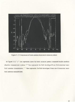
Figure 5.12 Comparison of horn antenna horizontal radiation pattern

In Figure 5.12 " ,/-" line represents direct far-field radiation pattern measured inside anechoic

chamber measurement system; "-" line represents far-field developed from 2-dimensional near­

field antenna measurement; ''." line represents far-field developed from one-dimensional near­

field antenna measurement.

69

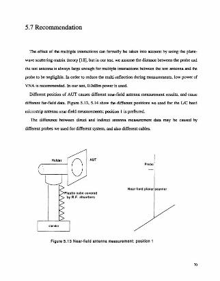
5.7 Recommendation

The effect of the multiple interact ions can Conn ally be take n into account by us ing the plane­

wave scartering-marrix theory [18J. but in our lest. we assume the distance between the probe and

the test antenna is always large enough for multiple interactions between the test ante nna and the

probeto be negligible . In order to reduce the multi-reflecti on during measurements. low power of

VNA is recommended. In our test. O.OdBm power is used.

Differe nt position of AUT causes different near-field antenna measurement results . and cause

different far-field data. Figure 5.13. 5.14 show the different positions we used for the UC band

microstrip antenna near-field measu remen ts; position 1 is preferred.

The diffe rence between direc t and indirect antenna meas urement data may be caused by

diffe rent probeswe used for diffe rent system. and alsodifferent cab les.

~.,

ltu u, '", . ,,"'..b, R.F. lb 50rtI. r.

I l l nd. ,

IProbl

Figure 5.13 Near-field anlenna measurement: positio n 1

70

~I n l'UTi' ;1~~o"..

~I IU lie Wbe.::;~

by R.F. Ib

~-

. llnna mluuremlnt position 2Figure 5.14 Near-held Int

11

Chapter 6

Conclu sion and Future Works

6. \ Conclusion

A low cost near-fieldlfar-field antenna measurement system has been designed. built in C­

CO RE. Mem orial Univers ity of Newfoundland . Val idating was done by using direct far -field

antenna measurement system (C-CORE's anechoic chamber measurement system). One- and

two-dimensional near-field measurements are performed on lhe ~anar scanning plane in the

near-field, FFT algorithm is used in the development of the far-field radiation pattern.

Reasonable agreements arc observed between the data calculated from the near-field/far-field

measu rement and direct far-field data measured in C-CORE' s anechoic chamber measurement

system.

One-dimensiona! near-field antenna measurements are preferred when measuring horizontal

radiation patterns. One-dimensional ncar-field antenna measurements do not need probe­

co rrection, also they make the near-field/far -field measurement speed and data process speed fast

co mparing with two-dimensional near -field measurement.

The dataobtained from near·fjeldJfar-fleld measurements and those directly measured inside

the chamber validate both techniques.

The software package for the system is written in such a way mat it has a user friendly

interface.

72

6.2 Future works

All of the near-field measurement results we obtained, are perfonned outside of the cham ber.

If measure ments are perfonned inside the chamber. the near-field measurement results should be

better .

The far-field radiation patterns which are obtained from two-dimens ional near-fie ld

measureme nts do not apply probe correctio n. Probe correction can be considered in the future

works .

73

References

[lJ Yahya Rahmar-Samii and Mark S. Gatti• • Far-field patterns of space bome antennas from

plane-polar near-field measuremen ts", IEEE trans . on Antennas and propagatio n. Vol. Ap-33.

No.6, pp. 638-648 . June 1985.

[2] Dan Slater, "Near-field antenna measurements", Artech House. me.• 1991.

[3] Gary E. Evans. "Antenna meas urement techniques ". ArtechHouse . Inc., 1990.

[4J Thod..ild B. Hansen. and D. Yaghjain. "Planar near-field scasnn ing in the time domai n, Pan

I: Fonnulation ".IEEE Trans. on Antenna and Propagui on. Vol. 42, No. 9, September 1994.

[5] Arthur D. Yaghjian, •An overview of near-fie ld antenna measurements", IEEE trans.

antenna and propagation. Vol. AP-34. No. I, pp. 1280-1291. January 1986.

[6} Richard C. Johnson. H. Allen Ecker . and J. Searc y Hollis, "Determi nation of far-field antenna

patterns from near-field measurements", Proc. of The IEEE. Vol. 6 1, No. 12. pp. 1668-1694 ,

December 1973.

[7] Yahya Rahmat-S amii , Lawrence L Williams. and Raben G. Yaccari no. "The UOA bi-polar

planar -near-field antenna measure ment and diagnosti cs range". IEEE Antenna & Propagatio n

Magazi ne. Vol. 37. No.6. Decembe r 1995.

"

(8) Y.T. 1.0 & S.W. Lee. "Antenna handbook" , Volume tv. Oaprnan & Hall, New York. NY.

1993.

(9] Y.T. 1.0 & s.w. Lee. MAnlenna handbook" , Volume L Chapman & Hall. New York. NY,

1993.

[10] E. S. Gillespie . "Measureroer u of antenna radiation characteristics on far-field ranges" , in

A...Unrla handbook , Edited by Y.T.Lo & S.W.Lee, Van Nostrand Reinhold Company. New York.

1993.

(11) "IEEE Sund.1rd Test Procedures for Antenna ", The Institute of Electrical and Electro nics

Engineen. Inc., 1979.

(12] Paul F. Wacke r, "Unified theory of near-field analysis and measurement: nonmathematical

discuss ion", IEEE Trans . on antenna and propagation , Vol. AP-30. No. I, pp. 99· 101. January

1982.

(131 Johnson J. H. Wang, NAnexamination of the theory and practices of planar near-field

measurement", IEEE Trans . on antenna and propaga tion, Vol. 36 . No.6. pp. 146-153, June 1988.

(l 4) Edward B. Joy and Demetrius T. Paris, "Spatial Sam pling and filtering in near-field

measurements", IEEE Trans . on Antenna andpropagation , Vol. AP·20 , No.3, pp. 253-26 1, May

1972.

( IS] L Olen and OJ .Edwards, "Applications of non-unifonn sampling techniques and fast

fourier transforms in plane near field antenna measurements ", Proc . 8th Int Conf. on Antennas

and Propagatio n. Edinburgh, U.K.. pp. 311-314, 1993 ,

[ 16] Mark S. Gatti and Yahya Rahmat-Sami i, "FFf applications to plane-polar near-field ante nna

measurements", IEEE Trans. on Antenna and propagati on, Vol. 36, No.6, pp. 181-791, June

1988.

"

(171 Edward B. Joy, "Near -field range qualification melhodology~ , IEEE Tran s. o n antenna and

propagation. Vol. 36. No.6, pp. 836-844 , June 1988.

(18) Thortild 8 . Hansen. -Form ulation of probe<errected planar near-field scann ing in the time

domain", IEEE Trans . on Antenna and Propagation. Vol. 43, No.6, June t99S

(19 ) Arthur D. Yaghjian. "Probe correction for near-field anten na meas urements". in Proc.

Antenna App licat ion Symp.• Univ, Illinois, Sept. 1984

[20] Constantine A. Balan ls, "Antenna theory analysis and design" , John Wiley & Son s. 1982.

[2 1] Michael H. Francis, Allen C. Newell , Kenneth R Grimm. John Hoffman. and Helmut E.

Schrank. "Comparison of ultralow -sidelobe-antenna far-field patterns using the plan ar-near-field

method and the far-field method ",1EEE Antenna and Propagation Maguine, Vol . 37. No.6, 1'1'.

7-15 , December 1995 .

[22J ~Model 360 Vecto r Network Analyzer system operation manual". Wiltron

{23] ~ModeI360 Vector Network.Analyzer system apm programm ing manual ", Wil tron

[24] Uo yd heff ord, -A prototype planar scanner for near field measuring system", Engineerin g

project 8800, MUN. Apri l 1996.

(2S] Raben E. Co llin, " Antenna and rsdtc weve propagation" , McGraw-ffill, Ine., 1985 .

(26) Dave Butt. S .A.Saoudy, -OCvelopment of an UC band microstrip antenna for satellite

synthe tic aperture radar" , NECE C'96, St. John 's, NF, Canada. Ma y 1996.

7'

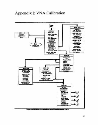
Appendix I: VNA Calibration

....""............""­~,.........""""­"""""'"-...-""""'"-""--..."""-""....---"''''''''

--~....-~-~....­,n""

- ..""'"~-=::r~K

"""'":0=-..,..==-

-­"".......,_..."""- ""...."".......,.........-...,~..­""'"'''''''''...........­.... .....­_ ..---­............,

71

~ ~ ~ ~--... -~ -... _............~ ......""'" _....~-""'-

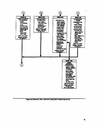
cou_ .....""" ~w .... """-- ~ ...""""""'" = ... ==... - """"""'""""""'... """'- .....-- ~== COl."'" """....

~=.-... -."...

~: -- """""'...""""""'" ......-~011"" · =-""'... """......NEXTCALSlU' """.... 'MU. .......T IlI

~~ """""'... =:MG......-,"""on-. ~0Hz......... i-'........." -..."'".....""".... ~~-.........."'- I~

!__ OM

0 ---........,..=A~"'.....--"""""'..."""...=.......,.,..,.""~............................"''''''''""nnw"""",

"

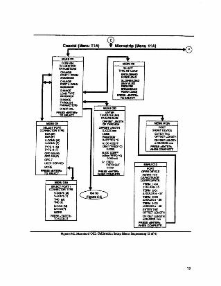
~ MJcrOWlp (Menu llA)

=-"'''''''--""""""......­IIM'I'AUO=.."""""'"~~dNJEJb

~

"'""""'"...................1'ORT1C1OHN

""""""'".......~CONN.......-"'"""""""'"=..............""""'-......­"''''-'CT

.,"'"."«<T""""""''''''''''''''-,.,-'""''''''''''""""""TYPI!!NIMJTYPEN(Fj

"""'''''~Cf)~_m

"'"'......~~lOR:LECT

=""".CONHtctoRlYI'E

""""""""""""'"""""""'":t, .... CM)U_""'",""",4"",""''''-'CT

""'"~""u"''',.............."""""""'""'''''''''''''"""""""""""'"-­EQUA.'TIC*:.......,-cA;DCCClEFF""':;;::"''<1I:OCCClEFF

1'*':.~'eI

C:FAEO

='"""~~

"""""'"'''''''.=~~~.....­......"""""

"""'"""',....,.........'""""""'"~o....""",..,:I:~lI"""...:lXXXJOt. ·:l7

~~311

"""""tiOOtJOC. ·"........"""""""'"........"""'"=-=~

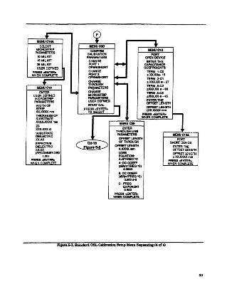
~ ~IllENUctlA .,"""C, ..... COIlMENUC1 2MlCFlOS'mIP """"...p""""",,, <:AU"'''''''' PORT

IO"' LKrT """'""'" OO'ENDEW>E15"L ICIT - ~

EmER ....25 MIL KIT ""R" """""""""USER DEFINED n """"'""'" """"",.,.,.

PRESS......... """'" """,-COWHEHCOMPl.ETI! POAT, ;: :txx.xx..l l.-- """"'""'" """~.

"""'" :tlOOOOC. · Z1""""'... """"'"MEHUct. .........,.,.. zxxx.xx • . 3lI

''''''' aw.e.""""'"USERoe:rtl EO ~p zxxx.xx . ...

M1CAOST1'llP ..............EmERTH'"""""'AS USER DEFINeD ......"""'".."..OF ...... CAl. h ".,..,"""'"

~-PRESS clEHfDb. =-OC.REC2 "........... 1""CXH"'OF

(1...............

'" esrwre=- ..... cot

~. '"""THAOUGHUNEsu.........

"""'""'" ..... .....~C1RC OF.......... ""'"e...""'"

OF.....,... SHORT DEVICE......"'" _........ omET...... """'","'XX """""- OFFSErL.DfQTHlRECONMENoeD "'" OFFSETLENOTH..." = :OC .""""""-PRESS <£NTEFb PRESS........

WHEN COMPLETE kOC COEFF _ ENCCt.lPl.E'Mlara:=m OClI :OCCOEFl"(dIW{m'FREQ"C).....C: l'l'lEO=-=~

Appendix II: GPIB Commands - Calibration

QIIII Cot......... .....-....---~ All; AIt. ..... AFl:_.NIL. -.IIEQ,"

CIt CIt. ceo _, ...CC1_~en.Q'3, CfC, CfI(, CFN.CfII, en.Cfl; CI'V,._CIa, CIIC, cue. cue. CIa, CIN.CND, QQ, .... CCN. ceo_~ cos_~ ClI'. CllI. ewe.DfC,llFD,DfQ_ ~"'FIlC,""_ ~__~FIIS_~ ...... ICEC,_11.,_~w_~w_uz_ ~ ...........Ul2,LIa,LTC.LTII,LlW. MCS,NOC. oeM.PIC. P2C, AOl. IU. AlII. RDL_~ RPC, ....S80_~__~ IlCIl,IH'_~

8HZ_~ lUI. tal. me. 1llI. lfE.1R. 1\lt"uss_~ usw_~usz_~ U,.. U, I, ll2ll.Y«lO_~WICll.WIQ

II