- Bogotá - Colombia - Bogotá - Colombia - Bogotá - Colombia - Bogotá - Colombia - Bogotá - Colombia - Bogotá - Colombia - Bogotá - Colombia - Bogotá - Colombia - Bogotá -

An Introductory Review of a Structural VAR-XEstimation and Applications∗

Sergio Ocamposocampdi@banrep.gov.co

Norberto Rodrígueznrodrini@banrep.gov.co

Macroeconomic Modeling Department, Banco de la República.

Abstract

This document presents how to estimate and implement a structural VAR-X model under long run and impactidentification restrictions. Estimation by bayesian and maximum likelihood methods is presented. Applicationsof the structural VAR-X for impulse response functions to structural shocks, multiplier analysis of the exogenousvariables, forecast error variance decomposition and historical decomposition of the endogenous variables arealso described, as well as a method for computing HPD regions in a bayesian context. Some of the conceptsare exemplified with an application to US data.

Keywords: S-VAR, B-VAR, VAR-X, IRF, FEVD, historical decomposition.JEL Classification: C11, C18, C32.

The use of VAR-X and structural VAR-X models in econometrics is not new, yet textbooks andarticles that use them often fail to provide the reader a concise (and moreover useful) description ofhow to implement these models (Lütkepohl (2005) constitutes an exception of this statement). The useof bayesian techniques in the estimation of VAR-X models is also largely neglected from the literature,as is the construction of the historical decomposition of the endogenous variables. This documentbuilds upon the S-VAR and B-VAR literature and its purpose is to present a review of some of thebasic features that accompany the implementation of a structural VAR-X model.

Section 1 presents the notation and general setup to be followed throughout the document. Section2 discuses the identification of structural shocks in a VAR-X, with both long run restrictions, as inBlanchard and Quah (1989), and impact restrictions, as in Sims (1980, 1986). Section 3 considers theestimation of the parameters by maximum likelihood and bayesian methods. In Section 4 it is shownhow to use the marginal density of the model for choosing the lag structure. Finally, in Section 5, fourof the possible applications of the model are presented, namely the construction of impulse responsefunctions to structural shocks, multiplier analysis of the exogenous variables, forecast error variancedecomposition and historical decomposition of the endogenous variables. Appendix A exemplifiessome of the concepts developed in the document using Galí (1999)’s structural VAR augmented withoil prices as an exogenous variable.

1 General setup

In all sections the case of a structural VAR-X whose reduced form is a VAR-X(p, q) will be considered.It is assumed that the system has n endogenous variables (yt) and m exogenous variables (xt). The

∗The results and opinions expressed in this document do not compromise in any way Banco de la República or itsboard of directors. We wish to thank Eliana González, Martha Misas, Andrés González, Luis Fernando Melo, andChristian Bustamente for useful comments on earlier drafts of this document, of course, all remaining errors are our own.

1

2 Identification of structural shocks in a VAR-X 2

variables in yt and xt may be in levels or in first differences, this depends on the characteristics of thedata, the purpose of the study, and the identification strategy, in all cases no co-integration is assumed.The reduced form of the structural model includes the first p lags of the endogenous variables, thecontemporaneous values and first q lags of the exogenous variables and a constant vector.1 Under thisspecification it is assumed that the model is stable and presents white-noise Gaussian residuals (et),i.e. et

iid∼ N (0,Σ).The reduced form VAR-X can be represented as in equation (1) or equation (2), where v is a

n-vector, Bi are (n× n) matrices and Θi are (n×m) matrices. In equation (2) one has B (L) =B1L+ . . .+BpL

p and Θ (L) = Θ0 + . . .+ ΘqLq, both matrices of polynomials in the lag operator L.

yt = v +B1yt−1 + . . .+Bpyt−p + Θ0xt + . . .+ Θqxt−q + et (1)yt = v +B (L) yt + Θ (L)xt + et (2)

Defining Ψ (L) = Ψ0 + Ψ1L+ . . . = [I −B (L)]−1 with Ψ0 = I as an infinite polynomial on the lag

operator L, one has the VMA-X representation of the model, equation (3).2

yt = Ψ (1) v + Ψ (L) Θ (L)xt + Ψ (L) et (3)

Finally, there is a structural VAR-X model associated with the equations above, most of theapplications are obtained from it, for example those covered in Section 5. Instead of the residuals(e), which can be correlated among them, the structural model contains structural disturbances witheconomic interpretation (ε), this is what makes it useful for policy analysis. It will be convenient torepresent the model by its VMA-X form, equation (4),

yt = µ+ C (L) εt + Λ (L)xt (4)

where the endogenous variables are expressed as a function of a constant n-vector (µ), and the currentand past values of the structural shocks (ε) and the exogenous variables. It is assumed that ε is avector of white noise Gaussian disturbances with identity covariance matrix, i.e. εt

iid∼ N (0, I). BothC (L) and Λ (L) are infinite polynomials in the lag operator L, each matrix of C (L) (C0, C1, . . .) is ofsize (n× n), and each matrix of Λ (L) (Λ0,Λ1, . . .) is of size (n×m).

2 Identification of structural shocks in a VAR-X

The identification of structural shocks is understood here as a procedure which enables the econometri-cian to obtain the parameters of a structural VAR-X from the estimated parameters of the reduced formof the model. As will be clear from the exposition below, the identification in presence of exogenousvariables is no different from what is usually done in the S-VAR literature.

Equating (3) and (4) one has:

µ+ Λ (L)xt + C (L) εt = Ψ (1) v + Ψ (L) Θ (L)xt + Ψ (L) et

then the following equalities can be inferred:1 The lag structure of the exogenous variables may be relaxed allowing different lags for each variable. This complicates

the estimation and is not done here for simplicity. Also, the constant vector or intercept may be omitted according tothe characteristics of the series used.

2 The models stability condition implies that Ψ (1) =

[I −

p∑i=1

Bi

]−1

exist and is finite.

2 Identification of structural shocks in a VAR-X 3

µ = Ψ (1) v (5)Λ (L) = Ψ (L) Θ (L) (6)

C (L) εt = Ψ (L) et (7)

Since the parameters in v, B (L) and Θ (L) can be estimated from the reduced form VAR-Xrepresentation, the values of µ and Λ (L) are also known.3 Only the parameters in C (L) are left to beidentified, the identification depends on the type of restrictions to be imposed. From equations (5), (6)and (7) is clear that the inclusion of exogenous variables in the model has no effect in the identificationof the structural shocks. Equation (7) also holds for a structural VAR model.

The identification restrictions to be imposed over C (L) may take several forms. Since there isnothing different in the identification between the case presented here and the S-VAR literature,we cover only two types of identification procedures, namely: impact and long run restrictions thatallow the use of the Cholesky decomposition. It is also possible that the economic theory points atrestrictions that make impossible a representation in which the Cholesky decomposition can be used, orthat the number of restrictions exceeds whats needed for exact identification. Both cases complicatethe estimation of the model, and the second one (over-identification) makes possible to carry outtest over the restrictions imposed. For a more comprehensive treatment of this problems we refer toAmisano and Giannini (1997).

There is another identification strategy that won’t be covered in this document, identification bysign restrictions over some of the impulse response functions. This kind of identification allows toavoid some puzzles that commonly arise in the VAR literature. References to this can be found inUhlig (2005), Mountford and Uhlig (2009), Canova and De Nicolo (2002), Canova and Pappa (2007)and preceding working papers of those articles originally presented in the late 1990’s. More recently,the work of Moon et al. (2011) presents how to conduct inference over impulse response functions withsign restrictions, both by classical and bayesian methods.

2.1 Identification by impact restrictionsIn Sims (1980, 1986) the identification by impact restrictions is proposed, the idea behind it is thatequation (7) is equating two polynomial in the lag operator L, for them to be equal it must be thecase that:

CiLiεt = ΨiL

iet

Ciεt = Ψiet (8)

Equation (8) holds for all i, in particular it holds for i = 0. Knowing that Ψ0 = I, the followingresult is obtained:

C0εt = et (9)

then, by taking the variance on both sides one gets:

C0C′

0 = Σ (10)

Since Σ is a symmetric, positive definite matrix it is not possible to infer in an unique form theparameters of C0 from equation (10), restrictions over the parameters of C0 have to be imposed.Because C0 measures the impact effect of the structural shocks over the endogenous variables, those

3 Lütkepohl (2005) presents methods for obtaining the matrices in Ψ (L) and the product Ψ (L) Θ (L) recursively inSections 2.1.2 and 10.6, respectively. Ψ (1) is easily computed by taking the inverse on I −B1 − . . .−Bp.

2 Identification of structural shocks in a VAR-X 4

restrictions are called here impact restrictions. Following Sims (1980), the restrictions to be imposedensure that C0 is a triangular matrix, this allows to use the Cholesky decomposition of Σ to obtainthe non-zero elements of C0. This amount of restrictions account n × (n − 1)/2 and make the modeljust identifiable.

Once C0 is known, equations (8) and (9) can be used to calculate Ci for all i as:

Ci = ΨiC0 (11)

The steps for the identification by impact restrictions are summarized in Algorithm 1.

Algorithm 1 Identification by impact restrictions

1. Estimate the reduced form of the VAR-X.

2. Calculate the VMA-X representation of the model (matrices Ψi) and the covariance matrix ofthe reduced form disturbances e (matrix Σ).

3. From the Cholesky decomposition of Σ calculate matrix C0 (equation 10).

C0 = chol (Σ)

4. For i = 1, . . . , R, with R given, use equation 11 to calculate the matrices Ci.

Ci = ΨiC0

Step 4 completes the identification in the sense that all matrices of the structural VMA-X are known.

2.2 Identification by long run restrictionsAnother way to identify the matrices of the structural VMA-X is to impose restrictions on the longrun impact of the shocks over the endogenous variables. This method is proposed in Blanchard andQuah (1989). For the model under consideration, if the variables in yt are in differences, the matrix

C (1) =∞∑i=0

Ci measures the long run impact of the structural shocks over the levels of the variables.4

Matrix C (1) is obtained by evaluating equation (7) in L = 1. As in the case of impact restrictions,the variance of each side of the equation is taken, the result is:

C (1)C′(1) = Ψ (1) ΣΨ

′(1) (12)

Again, since Ψ (1) ΣΨ′(1) is a symmetric, positive definite matrix it is not possible to infer the

parameters of C (1) from equation (12), restrictions over the parameters of C (1) have to be imposed.It is conveniently assumed that those restrictions make C (1) a triangular matrix, as before, this allowsto use the Cholesky decomposition to calculate the non-zero elements of C (1). Again, this amount ofrestrictions account n× (n− 1)/2 and make the model just identifiable.

Finally, it is possible to use C (1) to calculate the parameters in the C0 matrix, with it, thematrices Ci for i > 0 are obtained as in the identification by impact restrictions. Combining (10) with(7) evaluated in L = 1 the following expression for C0 is derived:

4 Of course, not all the variables of yt must be in differences, but the only meaningful restrictions are those imposedover variables that enter the model in that way. We restrict our attention to a case in which there are no variables inlevels in yt.

3 Estimation 5

C0 = [Ψ (1)]−1C (1) (13)

The steps for the identification by long run restrictions are summarized in Algorithm 2.

Algorithm 2 Identification by long run restrictions

1. Estimate the reduced form of the VAR-X.

2. Calculate the VMA-X representation of the model (matrices Ψi) and the covariance matrix ofthe reduced form disturbances e (matrix Σ).

3. From the Cholesky decomposition of Ψ (1) ΣΨ′(1) calculate matrix C (1) (equation 12).

C (1) = chol(

Ψ (1) ΣΨ′(1))

4. With the matrices of long run effects of the reduced form, Ψ (1), and structural shocks, C (1),calculate the matrix of contemporaneous effects of the structural shocks, C0 (equation 13).

C0 = [Ψ (1)]−1C (1)

5. For i = 1, . . . , R, with R sufficiently large, use equation (11) to calculate the matrices Ci.

Ci = ΨiC0

Step 5 completes the identification in the sense that all matrices of the structural VMA-X are known.

3 Estimation

The estimation of the parameters of the VAR-X can be carried out by maximum likelihood or bayesianmethods, as will become clear it is convenient to write the model in a more compact form. FollowingZellner (1996) and Bauwens et al. (2000), equation (1), for a sample of T observations, plus a fixedpresample, can be written as:

Y = ZΓ + E (14)

where Y =

y′

1...y′

t...y′

T

, Z =

1 y′

0 . . . y′

−(p−1) x′

1 . . . x′

1−q...1 y

′

t−1 . . . y′

t−p x′

t . . . x′

t−q...1 y

′

T−1 . . . y′

T−p x′

T . . . x′

T−q

, E =

e′

1...e′

t...e′

T

and Γ =

v′

B′

1...B′

p

Θ’o...

Θ′

q

.

For convenience we define the auxiliary variable k = (1 + np+m (q + 1)) as the total number ofregressors. The matrices sizes are as follow: Y is a (T × n) matrix, Z a (T × k) matrix, E a (T × n)matrix and Γ a (k × n) matrix.

Equation (14) is useful because it allows to represent the VAR-X model as a multivariate linearregression model, with it the likelihood function is derived. The parameters can be obtained bymaximizing that function or by means of Bayes theorem.

3 Estimation 6

3.1 The likelihood functionFrom equation (14) one derives the likelihood function for the error terms. Since et ∼ N (0,Σ),one has: E ∼ MN (0,Σ⊗ I), a matricvariate normal distribution with I the identity matrix withdimension (T × T ). The following box defines the probability density function for the matricvariatenormal distribution.The matricvariate normal distributionThe probability density function of a (p× q) matrix X that follows a matricvariate normal distributionwith mean Mp×q and covariance matrix Qq×q ⊗ Pp×p (X ∼ MN (M,Q⊗ P )) is:

MNpdf (M,Q⊗ P ) ∝ |Q⊗ P |−12 exp

(−1

2[vec (X −M)]

′(Q⊗ P )

−1[vec (X −M)]

)(15)

Following Bauwens et al. (2000), the vec operator can be replaced by a trace operator (tr):

MNpdf (M,Q⊗ P ) ∝ |Q|−p2 |P |

−q2 exp

(−1

2tr(Q−1 (X −M)

′P−1 (X −M)

))(16)

Both representations of the matricvariate normal pdf are useful when dealing with the compact rep-resentation of the VAR-X model. Note that the equations above are only proportional to the actualprobability density function. The missing constant term has no effects in the estimation procedure.

Using the definition in the preceding box and applying it to E ∼ MN (0,Σ⊗ I) one gets thelikelihood function of the VAR-X model, conditioned to the path of the exogenous variables:

L ∝ |Σ|−T2 exp

(−1

2tr(

Σ−1E′E))

From (14) one has E = Y − ZΓ, replacing:

L ∝ |Σ|−T2 exp

(−1

2tr(

Σ−1 (Y − ZΓ)′(Y − ZΓ)

))Finally, after tedious algebraic manipulation, one gets to the following expression:

L ∝[|Σ|

−(T−k)2 exp

(−1

2tr(Σ−1S

))] [|Σ|

−k2 exp

(−1

2tr(

Σ−1(

Γ− Γ)′Z′Z(

Γ− Γ)))]

where Γ =(Z′Z)−1

Z′Y and S =

(Y − ZΓ

)′ (Y − ZΓ

).

One last thing is noted, the second factor of the right hand side of the last expression is proportionalto the pdf of a matricvariate normal distribution for Γ, and the first factor to the pdf of an inverseWishart distribution for Σ (see the box below). This allows an exact characterization of the likelihoodfunction as in equation (17).

L = iWpdf (S, T − k − n− 1)MNpdf

(Γ,Σ⊗

(Z′Z)−1

)(17)

The parameters of the VAR-X, Γ and Σ, can be estimated by maximizing equation (17). It can beshown that the result of the likelihood maximization gives:

Γml = Γ Σml = S

3 Estimation 7

The inverse Wishart distributionIf the variable X (a square, positive definite matrix of size q) is distributed iW (S, v), with parameterS (also a square, positive definite matrix of size q), and v degrees of freedom, then its probabilitydensity function

(iWpdf

)is given by:

iWpdf (S, v) =|S|

v2

2vq2 Γq

(v2

) |X|−(v+q+1)2 exp

(−1

2tr(X−1S

))(18)

where Γq (x) = πq(q−1)

4

q∏j=1

Γ(x+ 1−j

2

)is the multivariate Gamma function. It is useful to have an

expression for the mean and mode of the inverse Wishart distribution, these are given by:

Mean (X) =S

v − q − 1Mode (X) =

S

v + q + 1

3.2 Bayesian estimationIf the estimation is carried out by bayesian methods the problem is to elect an adequate prior dis-tribution and, by means of Bayes theorem, obtain the posterior density function of the parameters.The use of bayesian methods is encouraged because they allow inference to be done conditional tothe sample, and in particular the sample size, giving a better sense of the uncertainty associated withthe parameters values; it also facilitate to compute moments not only for the parameters but for theirfunctions as is the case of the impulse responses, forecast error variance decomposition and others; itis also particularly useful to obtain a measure of skewness in this functions, specially for the policyimplications of the results. As mentioned in Koop (1992), the use of bayesian methods gives an exactfinite sample density for both the parameters and their functions.

The election of the prior is a sensitive issue and wont be discussed in this document, we shallrestrict our attention to the case of the Jeffreys non-informative prior (Jeffreys, 1961) which is widelyused in bayesian studies of vector auto-regressors. There are usually two reasons for its use. Thefirst one is that information about the reduced form parameters of the VAR-X model is scarce anddifficult to translate into an adequate prior distribution. The second is that it might be the case thatthe econometrician doesn’t want to include new information to the estimation but only wishes to usebayesian methods for inference purposes. Besides the two reasons already mentioned, the use of theJeffreys non-informative prior constitute a computational advantage because it allows a closed formrepresentation of the posterior density function, thus allowing to make draws for the parameters bydirect methods or by the Gibbs sampling algorithm (Geman and Geman, 1984).5

For a discussion of other usual prior distributions for VAR models we refer to Kadiyala and Karls-son (1997) and, more recently, to KociĘcki (2010) for the construction of feasible prior distributionsover impulse response in a structural VAR context. When the model is used for forecast purposesthe so called Minnesota prior is of particular interest, this prior is due to Litterman (1986), and isgeneralized in Kadiyala and Karlsson (1997) for allowing symmetry of the prior across equations. Thisgeneralization is recommended and is of easy implementation in the bayesian estimation of the model.It should me mentioned that the Minnesota prior is of little interest in the structural VAR-X context,principally because the model is conditioned to the path of the exogenous variables, adding difficultiesto the forecasting process.

In general the Jeffreys Prior for the linear regression parameters correspond to a constant for theparameters in Γ and for the covariance matrix a function of the form: |Σ|

−(n+1)2 , where n represents

the size of the covariance matrix. The prior distribution to be used is then:5 For an introduction to the use of the Gibbs sampling algorithm we refer to Casella and George (1992).

4 Marginal densities and lag structure 8

P (Γ,Σ) = C |Σ|−(n+1)

2 (19)

where C is the integrating constant of the distribution. Its actual value will be of no interest.The posterior is obtained from Bayes theorem as:

π (Γ,Σ|Y,Z) =L (Y,Z|Γ,Σ)P (Γ,Σ)

m (Y )(20)

where π (Γ,Σ|Y, Z) is the posterior distribution of the parameters given the data, L (Y,Z|Γ,Σ) is thelikelihood function, P (Γ,Σ) is the prior distribution of the parameters and m (Y ) the marginal densityof the model. The value and use of the marginal density is discussed in Section 4 and will be omittedin the current Section.

Combining equations (17), (19) and (20) one gets an exact representation of the posterior functionas the product of the pdf of an inverse Wishart distribution and the pdf of a matricvariate normaldistribution:

π (Γ,Σ|Y,Z) = iWpdf (S, T − k)MNpdf

(Γ,Σ⊗

(Z′Z)−1

)(21)

Equation (21) implies that Σ follows an inverse Wishart distribution with parameters S and T −k,and that the distribution of Γ given Σ is matricvariate normal with mean Γ and covariance matrix

Σ⊗(Z′Z)−1

. The following two equations formalize the former statement:

Σ|Y,Z ∼ iWpdf (S, T − k) Γ|Σ, Y, Z ∼ MNpdf

(Γ,Σ⊗

(Z′Z)−1

)Although further work can be done to obtain the unconditional distribution of Γ it is not necessary

to do so. Because equation (21) is an exact representation of the parameters distribution function, itcan be used to generate draws of them, moreover it can be used to compute any moment or statisticof interest, this can be done by means of the Gibbs sampling algorithm.

4 Marginal densities and lag structure

The marginal density (m (Y )) can be easily obtained under the Jeffreys prior and can be used afterwardfor purposes of model comparison. The marginal density gives the probability that the data is generatedby a particular model, eliminating the uncertainty due to the parameters values. Because of this m (Y )is often used for model comparison by means of the Bayes factor: the ratio between the marginaldensities of two different models that explain the same set of data (BF12 = m(Y |M1)/m(Y |M2)). If theBayes factor is bigger than one then the first model (M1) would be preferred.

From Bayes theorem (equation 20) the marginal density of the data, given the model, is:

m (Y ) =L (Y, Z|Γ,Σ)P (Γ,Σ)

π (Γ,Σ|Y, Z)(22)

its value is obtained by replacing for the actual forms of the likelihood, prior and posterior functions(equations 17, 19 and 21 respectively):

m (Y ) =Γn(T−k

2

)Γn(T−k−n−1

2

) |S|−n−12 2

n(n+1)2 C (23)

4 Marginal densities and lag structure 9

Algorithm 3 Bayesian estimation

1. Select the specification for the reduced form VAR-X, that is to chose values of p (endogenousvariables lags) and q (exogenous variables lags) such that the residuals of the VAR-X (e) havewithe noise properties. With this the following variables are obtained: T, p, q, k, where:

k = 1 + np+m (q + 1)

2. Calculate the values of Γ, S with the data (Y,Z) as:

Γ =(Z′Z)−1

Z′Y S =

(Y − ZΓ

)′ (Y − ZΓ

)3. Generate a draw for the covariance matrix of the reduced form VAR-X (Σ) from an inverse

Wishart distribution with parameter S and T − k degrees of freedom.

Σ ∼ iWpdf (S, T − k)

4. Generate a draw for the parameters of the reduced form VAR-X (Γ) from a matricvariate normal

distribution with mean Γ and covariance matrix Σ⊗(Z′Z)−1

.

Γ|Σ ∼ MNpdf

(Γ,Σ⊗

(Z′Z)−1

)5. Repeat steps 2-3 as many times as desired, save the values of each draw.

The draws generated (step 4) can be used to compute moments of the parameters.For every draw the corresponding structural parameters, impulse responses functions, etc. can becomputed, then, their moments and statistics can also be computed.The algorithms for generating draws for the inverse Wishart and matricvariate normal distributionsare presented in Bauwens et al. (2000), Appendix B.

Although the exact value of the marginal density for a given model cannot be known without theconstant C, this is no crucial for model comparison if the only difference between the models is in theirlag structure. In that case the constant C is the same for both models, and the difference between themarginal density of one specification or another arises only in the first two factors of the right hand

side of equation (23)[

Γn(T−k2 )

Γn(T−k−n−12 )

|S|−n−1

2

]. When computing the Bayes factor for any pair of models

the result will be given by those factors alone.The Bayes factor between a model, M1, with k1 regressors and residual covariance matrix S1, and

another model, M2, with k2 regressors and residual covariance matrix S2, can be reduced to:

BF12 =m (Y |M1)

m (Y |M2)=

Γn(T−k1

2

)Γn(T−k1−n−1

2

) |S1|−n−1

2 2n(n+1)

2 C

BF12 =

Γn(T−k12 )

Γn(T−k1−n−12 )

|S1|−n−1

2

Γn(T−k22 )

Γn(T−k2−n−12 )

|S2|−n−1

2

(24)

5 Applications 10

5 Applications

There are several applications for the structural VAR-X, all of them useful for policy analysis. In thisSection four of those applications are covered, they all use the structural VMA-X representation of themodel (equation 4).

5.1 Impulse response functions (IRF), Multiplier analysis (MA), and Forecasterror variance decomposition (FEVD)

Impulse response functions (IRF) and multiplier analysis (MA) can be constructed from the matrices inC (L) and Λ (L). The IRF shows the endogenous variables response to a unitary change in a structuralshock, in an analogous way the MA shows the response to a change in an exogenous variable. Theconstruction is simple and is based on the interpretations of the elements of the matrices in C (L) andΛ (L).

For the construction of the IRF consider matrix Ch. The elements of this matrix measure theeffect of the structural shocks over the endogenous variables h periods ahead, thus cijh (i-th row, j-thcolumn) measures the response of the i-th variable to a unitary change in the j-th shock h periodsahead. The IRF for the i-th variable to a change in j-th shock is constructed by collecting elementscijh for h = 0, 1, . . . ,H, with H the IRF horizon.

Matrices Ch are obtained from the reduced form parameters according to the type of identificationrestrictions (see Section 2). For a more detailed discussion on the construction and properties of theIRF we refer to Lütkepohl (2005), Section 2.3.2.

The MA is obtained in a similar fashion from the matrices Λh, these are also a function of thereduced form parameters.6 The interpretation is the same as before.

A number of methods for inference over the IRF and MA are available. If the estimation is carriedout by classical methods intervals for the IRF and MA can be computed by means of their asymptoticdistributions or by bootstrapping methods.7 Nevertheless, because the OLS estimators are biased,as proved in Nicholls and Pope (1988), the intervals that arise from both asymptotic theory andusual bootstrapping methods are also biased. As pointed out by Kilian (1998) this makes necessary toconduct the inference over IRF, and in this case over MA, correcting the bias and allowing for skewnessin the intervals. Skewness is common in the small sample distributions of the IRF and MA and arisesfrom the non-linearity of the function that maps the reduced form parameters to the IRF or MA. Adouble bootstrapping method that effectively corrects the bias and accounts for the skewness in theintervals is proposed in Kilian (1998).

In the context of bayesian estimation, it is noted that, applying Algorithm 1 or 2 for each draw ofthe reduced form parameters (Algorithm 3), the distribution for each cijh and λijh is obtained. With thedistribution function inference can be done over the point estimate of the IRF and MA. For instance,standard deviations in each horizon can be computed, as well as asymmetry measures and credible sets(or intervals), the bayesian analogue to a classical confidence interval.

In the following we shall restrict our attention to credible sets with minimum size (length), these arenamed Highest Posterior Density regions (HDP from now on). An (1− α) % HPD for the parameterθ is defined as the set C = {θ ∈ Θ : π (θ/Y ) ≥ k(α)}, where k(α) is the largest constant satisfyingP (C|y) =

´θπ (θ/Y ) dθ ≥ 1 − α.8 From the definition just given is clear that HPD regions are of

minimum size and that each value of θεC has a higher density (probability) than any value of θ outsidethe HPD. The second property makes possible direct probability statements about the likelihood of θfalling in C, i.e., “The probability that θ lies in C given the observed data Y is at least (1−α)%”, thiscontrast with the interpretation of the classical confidence intervals. An HPD region can be disjoint if

6 See Lütkepohl (2005), Section 10.67 The asymptotic distribution of the IRF and FEVD for a VAR is presented in Lütkepohl (1990). A widely used

non-parametric bootstrapping method is developed in Runkle (1987).8 Integration can be replaced by summation if θ is discrete.

5 Applications 11

Algorithm 4 Highest Posterior Density RegionsAs in Chen and Shao (1998), let

{θ(i), i = 1 , . . . , N

}be an ergodic sample of π (θ/Y ), the posterior

density function of parameter θ. π (θ/Y ) is assumed to be unimodal. The (1− α) % HPD is computedas follows:

1. Sort the values of θ(i). Define θ(j) as the j − th larger draw of the sample, so that:

θ(1) = miniε{1,...,N}

{θ(i)}

θ(N) = maxiε{1,...,N}

{θ(i)}

2. Define N = b(1− α)Nc the integer part of (1− α)N . The HPD will contain N values of θ.

3. Define C(j) =(θ(j) , θ(j+N)

)an interval in the domain of the parameter θ, for jε

{1, . . . , N −N

}.

Note that although C(j) contains always N draws of θ, its size may vary.

4. The HPD is obtained as the interval C(j) with minimum size. HPD (α) = C(j?), with j? suchthat:

θ(j?+N) − θ(j?) = minjε{1,...,N−N}

(θ(j+N) − θ(j)

)

the posterior density function (π (θ/Y )) is multimodal. If the posterior is symmetric, all HPD regionswill be symmetric about posterior mode (mean).

Koop (1992) presents a detailed revision of how to apply bayesian inference to the IRF in a structuralVAR context, his results can be easily adapted to the structural VAR-X model. Another reference onthe inference over IRF is Sims and Zha (1999). Here we present, in Algorithm 4, the method of Chenand Shao (1998) for computing HPD regions from the output of the Gibbs sampler.9

It is important to note that bayesian methods are by nature conditioned to the sample size and,because of that, avoid the problems of asymptotic theory in explaining the finite sample propertiesof the parameters functions, this includes the skewness of the IRF and MA distribution functions.Then, if the intervals are computed with the HPD, as in Chen and Shao (1998), they would be takinginto account the asymmetry in the same way as Kilians method. This is not the case for intervalscomputed using only standard deviations although, with them, skewness can be addressed as in Koop(1992), although bootstrap methods can be used to calculate approximate measures of this and othersmoments, for instance, skewness and kurtosis, Bayesian methods are preferable since exact measurescan be calculated.

Another application of the structural VAR-X model is the forecast error variance decomposition(FEVD), this is no different to the one usually presented in the structural VAR model. FEVD consistsin decomposing the variance of the forecast error of each endogenous variable h periods ahead, as withthe IRF, the matrices of C (L) are used for its construction. Note that, since the model is conditionedto the path of the exogenous variables, all of the forecast error variance is explained by the structuralshocks. Is because of this that the FEVD has no changes when applied in the structural VAR-X model.We refer to Lütkepohl (2005), Section 2.3.3, for the details of the construction of the FEVD. Again,if bayesian methods are used for the estimation of the VAR-X parameters, the density function of theFEVD can be obtained and several features of it can be explored, Koop (1992) also presents how toapply bayesian inference in this respect.

9 The method presented is only valid if the distribution of the parameters of interest is unimodal. For a more generaltreatment of the highest posterior density regions, including multimodal distributions, we refer to the work of Hyndman(1996).

5 Applications 12

5.2 Historical decomposition of the endogenous variables (HD)The historical decomposition (HD) consists in explaining the observed values of the endogenous vari-ables in terms of the structural shocks and the path of the exogenous variables. This kind of exerciseis present in the DSGE literature (for example, in Smets and Wouters (2007)) but mostly absent inthe structural VAR literature, being Canova (2007) an exception.10 Unlike the applications alreadypresented, the historical decomposition allows to make an statement over what has actually happenedto the series in the sample period, in terms of the recovered values for the structural shocks and theobserved paths of the exogenous variables. It allows to have all shocks and exogenous variables actingsimultaneously, thus making possible the comparison over the relative effects of them over the endoge-nous variables, this means that the HD is particularly useful when addressing the relative importanceof the shocks over some set of variables. The possibility of explaining the history of the endogenousvariables instead of what would happen if some hypothetical shock arrives in the absence of any otherdisturbance is at least appealing.

Here we describe a method for computing the HD in a structural VAR and structural VAR-Xcontext. The first case is covered in more detail and the second presented as an extension of the basicideas.

5.2.1 Historical decomposition for a structural VAR model

In a structural VAR context is clear, from the structural VMA representation of the model, thatvariations of the endogenous variables can only be explained by variations in the structural shocks.The HD uses the structural VMA representation in order to compute what the path of each endogenousvariable would have been conditioned to the presence of only one of the structural shocks. It isimportant to note that the interpretation of the HD in a stable VAR model is simpler than theinterpretation in a VAR-X. This is because in the former there is no need for a reference value thatindicates when a shock is influencing the path of the variables. In that case, the reference value isnaturally zero, and it is understood that deviations of the shocks below that value are interpreted asnegative shocks and deviations above as positive shocks. As we shall see, when dealing with exogenousvariables a reference value must be set, and its election is not necessarily “natural”.

Before the HD is computed it is necessary to recover the structural shocks from the estimation ofthe reduced form VAR. Define E = [e1 . . . et . . . eT ]

′as the matrix of all fitted residuals from the VAR

model (equation (14) in the absence of exogenous variables). Recalling equation (9), the matrix C0

can be used to recover the structural shocks from matrix E as in the following expression:

E = E(C′

0

)−1

(25)

Because zero is the reference value for the structural shocks the matrix E = [ε1 . . . εt . . . εT ]′can be

used directly for the HD.The HD is an in-sample exercise, thus is conditioned to the initial values of the series. It will be

useful to define the structural infinite VMA representation of the VAR model, as well as the structuralVMA representation conditional on the initial values of the endogenous variables, equations (26) and(27) respectively.

yt = µ+ C (L) εt (26)

yt =

t−1∑i=0

Ciεt−i +Kt (27)

10 Another exception is found in King and Morley (2007) where the historical decomposition of a structural VAR isused for computing a measure of the natural rate of unemployment for the US.

5 Applications 13

Note that in equation (26) the endogenous variables depend on an infinite number of past structuralshocks. In equation (27) the effect of all shocks that are realized previous to the sample is captured bythe initial values of the endogenous variables. The variable Kt is a function of those initial values andof the parameters of the reduced form model, Kt = ft

(y0 , . . . , y−(p−1)

). It measures the effect of the

initial values over the period t realization of the endogenous variables, thus the effect of all shocks thatoccurred before the sample. It is clear that if the VAR is stable Kt −→ µ for t sufficiently large, thisis because the shocks that are too far in the past have no effect in the current value of the variables.Kt will be refer to as the reference value of the historical decomposition.

Starting from the structural VMA representation, the objective is now to decompose the deviationsof yt from Kt into the effects of the current and past values of the structural shocks (εi for i from 1 to

t). The decomposition is made over the auxiliary variable yt = yt −Kt =t−1∑i=0

Ciεt−i. The information

needed to compute yt is contained in the first t matrices Ci and the first t rows of matrix E .The historical decomposition of the i-th variable of yt into the j-th shock is given by:

y(i,j)t =

t−1∑i=0

ciji εjt−i (28)

Note that it must hold that the sum over j is equal to the actual value of the i-th element of yt,

yit =n∑j=1

y(i,j)t . For t sufficiently large, when Kt is close to µ, y(i,j)

t can be interpreted as the deviation

of the i-th endogenous variable from its mean caused by the recovered sequence for the j-th structuralshock.

Finally, the endogenous variables can be decomposed as well. The historical decomposition for thei-th endogenous variable into the j-th shock is given by:

y(i,j)t = Ki

t + y(i,j)t = Ki

t +

t−1∑i=0

ciji εjt−i (29)

the new variable y(i,j)t is interpreted as what the i-th endogenous variable would have been if only

realizations of the j-th shock had occurred. The value of Kt can be obtained as a residual of thehistorical decomposition, since yt is known and yt can be computed from the sum of the HD or fromthe definition.

The HD of the endogenous variables (y(i,j)t ) can be also used to compute what transformations of

the variables would have been conditioned to the presence of only one shock. For instance, if the i-thvariable enters the model in quarterly differences, the HD for the annual differences or the level of theseries can be computed by applying to y(i,j)

t the same transformation used over yit, in this example, acumulative sum.

Algorithm 5 summarizes the steps carried out for the historical decomposition.

5.2.2 Historical decomposition for a structural VAR-X model

The structure already described applies also for a VAR-X model. The main difference is that now itsnecessary to determine a reference value for the exogenous variables.11 It shall be understand thatrealizations of the exogenous variables different to this value are what explain the fluctuations of theendogenous variables. We shall refer to xt as the reference value for the exogenous variables in t.

11 The reference value for the exogenous variables need not be a constant. It can be given by a linear trend, by thesample mean of the series,or by the initial value. When the exogenous variables enter the model in their differences, itmay seem natural to think in zero as a natural reference value, identifying fluctuations of the exogenous variables in ananalogous way to whats done with the structural shocks.

5 Applications 14

Algorithm 5 Historical decomposition for a structural VAR model

1. Estimate the parameters of the reduced form VAR.

(a) Save a matrix with all fitted residuals(E = [e1 . . . et . . . eT ]

′).

(b) Compute matrices Ci according to the identifying restrictions (Algorithm 1 or 2).

2. Compute the structural shocks(E = [ε1 . . . εt . . . εT ]

′)with matrix C0 and the fitted residuals of

the reduced form VAR:

E = E(C′

0

)−1

3. Compute the historical decomposition of the endogenous variables relative to Kt:

y(i,j)t =

t−1∑i=0

ciji εjt−i

4. Recover the values of Kt with the observed values of yt and the auxiliary variable yt:

Kt = yt − yt

5. Compute the historical decomposition of the endogenous variables:

y(i,j)t = Ki

t + y(i,j)t

Steps 3 and 5 are repeated for t = 1, 2, . . . , T , i = 1, . . . , n and j = 1, . . . , n. Step 4 is repeated fort = 1, 2, . . . , T .

As before, its necessary to present the structural VMA-X representation conditional to the initialvalues of the endogenous variables (equation 30), with Kt defined as above. It is also necessary toexpress the exogenous variables as deviations of the reference value, for this we define an auxiliaryvariable xt = xt − xt. Note that equation (30) can be written in terms of the new variable xt as in

equation (31). In the later, the new variable Kt =t−1∑i=0

Λixt−i +Kt has a role analogous to that of Kt

in the VAR context. Kt properties depend on those of xt and, therefore, it can’t be guaranteed thatit converges to any value.

yt =

t−1∑i=0

Ciεt−i +

t−1∑i=0

Λixt−i +Kt (30)

yt =

t−1∑i=0

Ciεt−i +

t−1∑i=0

Λixt−i + Kt (31)

The historical decomposition is now computed using matrices Ci, the recovered matrix of structuralshocks E , matrices Λi and the auxiliary variables xi, for i from 1 to T . Matrix E is still computed as inequation (25). The new reference value for the historical decomposition is Kt, and the decompositionis done to explain the deviations of the endogenous variables with respect to it as a function of thestructural shocks and deviations of the exogenous variables from their own reference value, xt. For

5 Applications 15

Algorithm 6 Historical decomposition for a structural VAR-X model

1. Estimate the parameters of the reduced form VAR-X.

(a) Save a matrix with all fitted residuals(E = [e1 . . . et . . . eT ]

′).

(b) Compute matrices Ci and Λi according to the identifying restrictions (Algorithm 1 or 2).

2. Compute the structural shocks(E = [ε1 . . . εt . . . εT ]

′)with matrix C0 and the fitted residuals of

the reduced form VAR-X:

E = E(C′

0

)−1

3. Compute the historical decomposition of the endogenous variables relative to Kt:

y(i,j)t =

t−1∑i=0

ciji εjt−i y

(i,k)t =

t−1∑i=0

λiki xkt−i

4. Recover the values of Kt with the observed values of yt and the auxiliary variable yt:

Kt = yt − yt

5. Compute the historical decomposition of the endogenous variables:

y(i,j)t = Ki

t + y(i,j)t y

(i,k)t = Ki

t + y(i,k)t

Steps 3 and 5 are repeated for t = 1, 2, . . . , T , i = 1, . . . , n , j = 1, . . . , n and k = 1, . . . ,m. Step 4 isrepeated for t = 1, 2, . . . , T .

notation, variable yt is redefined: yt = yt− Kt =t−1∑i=0

Ciεt−i +t−1∑i=0

Λixt−i. The decomposition of the i-th

variable of yt into the j-th shock is still given by equation (28), and the decomposition into the k-thexogenous variable is given by:

y(i,k)t =

t−1∑i=0

λiki xkt−i (32)

Variable y(i,k)t , for k from 1 to m, is interpreted as what the variable yit would have been if, in

the absence of shocks, only the k-th exogenous variable is allowed to deviate from its reference value.

As in the VAR model, it holds the following equation: yit =n∑j=1

y(i,j)t +

m∑k=1

y(i,k)t . The variable Kt is

recovered in the same way used before to recover Kt.The historical decomposition of the endogenous variables can be computed by using the recovered

values for Kt . The decomposition of the i-th variable into the effects of the j-th shock is still givenby equation (29), if Ki

t is replaced by Kit . The decomposition of the i-th variable into the deviations

of the k-th exogenous variable from its reference value is obtained from the following expression:

5 Applications 16

y(i,k)t = Ki

t + y(i,k)t (33)

Variable y(i,k)t has the same interpretation as y(i,k)

t but applied to the value of the endogenousvariable, and not to the deviation from the reference value.

Although the interpretation and use of the HD in exogenous variables may seem strange andimpractical, it is actually of great utility when the reference value for the exogenous variables is chosencorrectly. The following example describes a case in which the interpretation of the HD in exogenousvariables is more easily understood. Consider the case in which the exogenous variables are introducedin the model in their first differences. The person performing the study may be asking himself theeffects of the shocks and the changes in the exogenous variables over the endogenous variables. In thiscontext, the criteria or reference value for the exogenous variables arises naturally as a base scenario ofno change in the exogenous variables and no shocks. Under the described situation one has, for all t,xt = 0 and Kt = Kt. This also allows to interpret both y(i,k)

t and y(i,k)t as what would have happened

to the i-th endogenous variable if it were only for the changes of the k-th exogenous variable.Algorithm 6 summarizes the steps carried out for the historical decomposition in a structural

VAR-X setup.

References

Amisano, G. and Giannini, C. (1997). Topics in structural VAR econometrics. Springer.

Bauwens, L., Lubrano, M., and Richard, J.-F. (2000). Bayesian inference in dynamic econometricmodels. Oxford University Press.

Blanchard, O. J. and Quah, D. (1989). The dynamic effects of aggregate demand and supply distur-bances. American Economic Review, 79(4):655–73.

Canova, F. (2007). Methods for applied macroeconomic research. Number 13 in Princeton Series inApplied Mathematics. Princeton University Press.

Canova, F. and De Nicolo, G. (2002). Monetary disturbances matter for business fluctuations in theg-7. Journal of Monetary Economics, 49(6):1131–1159.

Canova, F. and Pappa, E. (2007). Price differentials in monetary unions: The role of fiscal shocks.Economic Journal, 117(520):713–737.

Casella, G. and George, E. I. (1992). Explaining the Gibbs sampler. The American Statistician,46(3):167–174.

Chen, M. and Shao, Q. (1998). Monte carlo estimation of bayesian credible and HPD intervals. Journalof Computational and Graphical Statistics, 8:69–92.

Galí, J. (1999). Technology, employment, and the business cycle: Do technology shocks explainaggregate fluctuations? American Economic Review, 89(1):249–271.

Geman, S. and Geman, D. (1984). Stochastic relaxation, Gibbs distributions, and the bayesian restora-tion of images. IEEE Transactions on Pattern Analysis and Machine Intelligence, 6:721–741.

Hyndman, R. J. (1996). Computing and graphing highest density regions. The American Statistician,50:120–126.

Jeffreys, H. (1961). Theory of probability. International Series of Monographs on Physics. ClarendonPress.

Kadiyala, K. R. and Karlsson, S. (1997). Numerical methods for estimation and inference in bayesianVAR-models. Journal of Applied Econometrics, 12(2):99–132.

5 Applications 17

Kilian, L. (1998). Small-sample confidence intervals for impulse response functions. The Review ofEconomics and Statistics, 80(2):218–230.

King, T. B. and Morley, J. (2007). In search of the natural rate of unemployment. Journal of MonetaryEconomics, 54(2):550–564.

KociĘcki, A. (2010). A prior for impulse responses in bayesian structural VAR models. Journal ofBusiness & Economic Statistics, 28(1):115–127.

Koop, G. (1992). Aggregate shocks and macroeconomic fluctuations: A bayesian approach. Journalof Applied Econometrics, 7(4):395–411.

Litterman, R. B. (1986). Forecasting with bayesian vector autoregressions-five years of experience.Journal of Business & Economic Statistics, 4(1):25–38.

Lütkepohl, H. (1990). Asymptotic distributions of impulse response functions and forecast error vari-ance decompositions of vector autoregressive models. The Review of Economics and Statistics,72(1):116–25.

Lütkepohl, H. (2005). New introduction to multiple time series analysis. Springer.

Moon, H. R., Schorfheide, F., Granziera, E., and Lee, M. (2011). Inference for VARs identified withsign restrictions. NBER Working Papers 17140, National Bureau of Economic Research, Inc.

Mountford, A. and Uhlig, H. (2009). What are the effects of fiscal policy shocks? Journal of AppliedEconometrics, 24(6):960–992.

Nicholls, D. F. and Pope, A. L. (1988). Bias in the estimation of multivariate autoregressions. Aus-tralian Journal of Statistics, 30A(1):296–309.

Runkle, D. E. (1987). Vector autoregressions and reality. Journal of Business & Economic Statistics,5(4):437–42.

Sims, C. A. (1980). Macroeconomics and reality. Econometrica, 48(1):1–48.

Sims, C. A. (1986). Are forecasting models usable for policy analysis? Quarterly Review, pages 2–16.

Sims, C. A. and Zha, T. (1999). Error bands for impulse responses. Econometrica, 67(5):1113–1156.

Smets, F. and Wouters, R. (2007). Shocks and frictions in US business cycles: A bayesian DSGEapproach. American Economic Review, 97(3):586–606.

Uhlig, H. (2005). What are the effects of monetary policy on output? results from an agnosticidentification procedure. Journal of Monetary Economics, 52(2):381–419.

Zellner, A. (1996). An introduction to bayesian inference in econometrics. Wiley Classics Library.John Wiley.

A An application 18

A An application

In this appendix some of the concepts presented in the document are exemplified by an application ofGalí (1999)’s structural VAR, augmented with oil prices as an exogenous variable. The exercise hasillustrative purposes only and does not mean to make any assessment on the economics involved.

The Appendix is organized as follows: first a description of the model to be used is made, thenthe lag structure of the reduced form VAR-X is chosen and the estimation described. Finally, impulseresponse functions, multiplier analysis and the historical decomposition are presented for one of themodel’s endogenous variables.

A.1 The model and the dataThe model used in this application is original from Galí (1999) and is a bi-variate system of laborproductivity and a labor measure.12 The labor productivity is defined as the ratio between product(GDP) and labor. The identification of the shocks is obtained by imposing long run restrictions ala Blanchard and Quah (1989). Two shocks are identified, a technology (productivity) shock and anon-technology shock, the former is assumed to be the only shock that can have long run effects on thelabor productivity. As pointed out in Galí (1999) this assumption is maintain in neoclassical growth,RBC and New-Keynesian models among others.

The model is augmented with oil prices as an exogenous variable with the only purpose of turningit into a structural VAR-X model, so that it can be used to illustrate some of the concepts of thedocument. As mentioned in Section 2 the presence of an exogenous variable doesn’t change theidentification of the structural shocks.

All variables are included in the model in their first differences, this is done partially as a conditionfor the long run identification (labor productivity) and partially because of the unit root behavior ofthe observed series. It should be clear that, in the notation of the document, n = 2 (the number ofendogenous variables) and m = 1 (the number of exogenous variables).

Noting by zt the labor productivity, lt the labor measure and pot the oil price, the reduced formrepresentation of the model is given by equation (1) with yt =

[∆zt ∆lt

]′and xt = ∆pot :

yt = v +B1yt−1 + . . .+Bpyt−p + Θ0xt + . . .+ Θqxt−q + et

In the last equation vector v is of size 2 × 1, matrices Bi are of size 2 × 2 for i = 1 : p and all Θj

are 2× 1 vectors. The structural VMA-X form of the model is given (as in equation (4)) by:

yt = µ+ C (L) εt + Λ (L)xt

with µ a 2 × 1 vector, each matrix of C (L) is of size 2 × 2, and the “coefficients” of Λ (L) are 2 × 1vectors. εt =

[εTt εNTt

]is the vector of structural shocks.

The identification assumption implies that C (1) is a lower triangular matrix, this allows us to usealgorithm 2 for the identification of the shocks and the matrices in C (L). Equations (5), (6) and (7)still hold.

The data set used to estimate the model consists in quarterly GDP, non-farm employees and oilprice series for the US economy that range from 1948Q4 to 1999Q1. The quarterly GDP is obtainedfrom the Bureau of Economic Analysis, and the non-farm employees and oil price from the FREDdatabase of the Federal Reserve Bank of St. Louis. GDP and non-farm employees are seasonallyadjusted. GDP is measured in billions of chained 2005 dollars, non-farm employees in thousands ofpersons and oil prices as the quarterly average of the WTI price in dollars per barrel.

12 Galí uses total hours worked in the non-farm sector as labor measure in the main exercise but also points at thenumber of employees as another possible labor measure, here we take the second option and use non-farm employees.

A An application 19

Tab. 1: Marginal Densities

m0 (Y ) m1 (Y ) m2 (Y ) m3 (Y ) m4 (Y ) m5 (Y ) m6 (Y )

6.1379 6.1268 6.1664 6.1817 6.2414 6.1733 6.1115The values presented are proportional to the marginal densities of the models by a factor of 1013C.

A.2 Lag structure and estimationChoosing the lag structure of the model consists in finding values for p and q so that the estimatedreduced form model satisfies some conditions. In this case we shall choose values for p and q so that theresiduals (et) are not auto-correlated.13 The tests indicate that four lags of the endogenous variablesare necessary for obtaining non-auto-correlated residuals (p = 4), this result is independent of the lagsof the exogenous variable. The change of the oil prices can be included only contemporary (q = 0) orwith up to six lags (q = 6).

Since any number of lags of the exogenous variables makes the residuals satisfy the desired condition,the marginal density of the different models (under the Jeffreys prior) is used to determined the valueof q. Each possible model only differs in the lags of exogenous variable, there are seven models indexedas mi (Y ) with i = 0 . . . 6. The marginal density for each model is computed as in equation (23):

mi (Y ) =Γn(T−ki

2

)Γn(T−ki−n−1

2

) |Si|−n−12 2

n(n+1)2 C

A presample is taken so that all models have the same effective T , since all have the same numberof endogenous variables (n = 2), the only difference between the marginal density of two models is inki (the total number of regressors) and Si (the estimated covariance of the residuals). Recalling from

Section 3: ki = (1 + np+m (qi + 1)) and Si =(Y − ZiΓi

)′ (Y − ZiΓi

).

Table 1 presents the results of the marginal densities, it is clear that the marginal density doesn’tincrease monotonically in the exogenous lag and that m4 (Y ) (q = 4) is preferred to the other mod-els. Then, the VAR-X model is estimated with four lags in both the endogenous and the exogenousvariables, and the contemporary value of the change in the oil price.

The estimation is carried out by bayesian methods under the Jeffreys prior as in Section 3.2.Algorithm 3 is applied to obtain 10,000 draws of the reduced form parameters, for every draw Algorithm2 is applied, along with the identification restriction over the technology shock, to obtain the parametersof the structural VMA-X representation of the model.

A.3 Impulse response functions and multiplier analysisFrom the output of the bayesian estimation of the model the impulse response function and multipliersare computed. Note that the distributions of the IRF and the multipliers are available since theestimation allows to obtain both for each draw of the reduced form parameters. This makes possibleto compute highest posterior density regions (HPD) as mentioned in Section 5.1. For doing so wepresented, in Algorithm 4, the steps to be carried out in the case in which the distribution of theIRF and the multipliers in every period is unimodal. Here we present only the response of labor to atechnology shock and a change in oil price as the posterior mean of the responses generated for each ofthe 10,000 draws of the parameters, the responses are presented along with HPD regions at 68% and90% probability.

Before presenting the HPD for the IRF and the multipliers its necessary to check if the distributionof the responses in every period are unimodal. Although no sufficient, a preliminary test of thementioned condition is to check the histograms of the IRF and the multipliers before computing the

13 The auto-correlation of the residual is tested whit Portmanteau tests at a 5% significance level. See Lütkepohl(2005), Section 4.4.3.

A An application 20

Fig. 1: Histograms

(a) IRF: Labor to tech shock at impact

−3 −2.5 −2 −1.5 −1 −0.5

x 10−3

0

50

100

150

200

250

300

350

(b) MA: Labor to oil price at impact

−0.02 −0.015 −0.01 −0.005 0 0.005 0.01 0.0150

50

100

150

200

250

300

350

Histograms of the response of labor to a technology shock and a change in the oil price at impact. The histograms are

obtained from 10000 draws of the parameters of the structural VAR-X model, and are computed with 100 bins.

HPD. Figure 1 presents the histograms for the response of labor to a technology shock (Figure 1a)and to a change in oil price (Figure 1b) at impact, the histograms for up to 20 periods ahead are alsochecked, but not presented. In all cases Algorithm 4 can be used.

The results are presented in Figure 2 and point to a decrease of labor in response to both a positivetechnology shock and an increase in oil prices, although the decrease is only significant for the responseto a technology shock. The response of labor to an increase in the oil price is never significant at 90%probability and only significant at 68% probability after period 5.

Fig. 2: IRF and MA

(a) IRF: Labor to tech shock

0 2 4 6 8 10 12 14 16 18 20−4.5

−4

−3.5

−3

−2.5

−2

−1.5

−1

−0.5

0x 10

−3

(b) MA: Labor to oil price at impact

0 2 4 6 8 10 12 14 16 18 20−0.07

−0.06

−0.05

−0.04

−0.03

−0.02

−0.01

0

0.01

0.02

Response of labor to a unitary technology shock and a unit change in the oil price. The point estimate (dark line) corresponds

to the posterior mean of the distribution of the IRF and the multipliers of labor, the distributions are obtained from 10000

draws of the parameters of the structural VAR-X model. HPD regions at 68% and 90% probability are presented as dark

and light areas correspondingly.

A.4 Historical decompositionFinally, the historical decomposition of labor into the two structural shocks and the changes in the oilprice is computed. As mentioned in Section 5.2 its necessary to fix a reference value for the exogenous

A An application 21

Fig. 3: Historical Decomposition - Labor in first difference

1960 1970 1980 1990−0.025

−0.02

−0.015

−0.01

−0.005

0

0.005

0.01

0.015

0.02

Tech Shock No−Tech Shock Oil Price

variable. Since the oil price enters the model in its first difference, the reference value will be set to zero(∀t xt = 0). This means that all changes in the oil price are understood by the model as innovationsto that variable.14 In this exercise all computations are carried out with the posterior mean of theparameters. Since the Jeffreys prior was used in the estimation, the posterior mean of the parametersequals their maximum likelihood values.

Applying Algorithm 6, steps 1 to 3, the historical decomposition for the first difference of labor(relative to Kt) is obtained, this is presented in Figure 3. Yet, the results are unsatisfactory, principallybecause the quarterly difference of labor lacks of a clear interpretation, its scale is not the one commonlyused and might be too volatile for allowing an easy understanding of the effects of the shocks.15

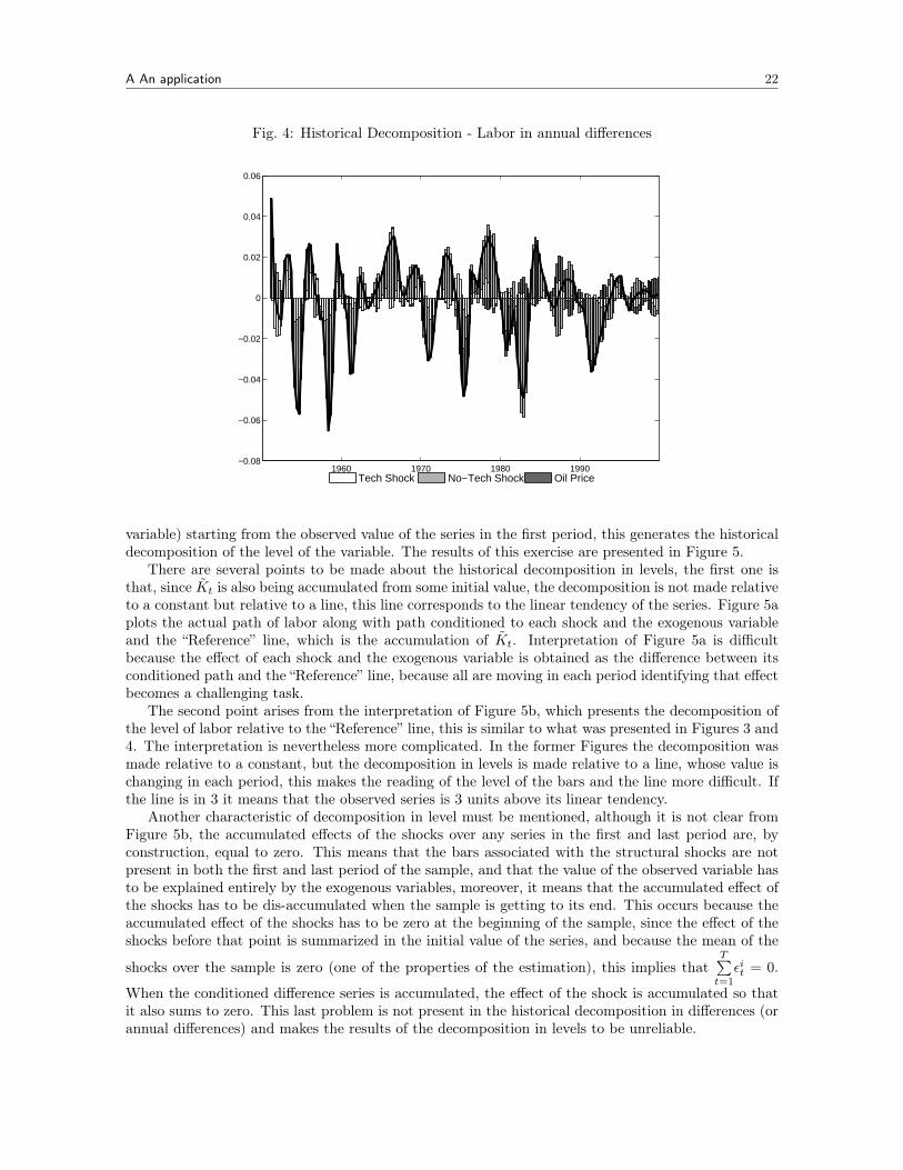
An alternative to the direct historical decomposition is to use the conditioned series (step 5 ofAlgorithm 6) to compute the historical decomposition of the annual differences of the series, this isdone by summing up the quarterly differences conditioned to each shock and the exogenous variable.The advantage of this transformation is that it allows for an easier interpretation of the historicaldecomposition, since the series is now less volatile and its level is more familiar for the researcher (thisis the case of the annual inflation rate or the annual GDP growth rate). The result is presented inFigure 4, it is clear that labor dynamics have been governed mostly by non-technology shocks in theperiod under consideration, with technology shocks and changes in the oil price having a minor effect.

Its worth to note that decomposing the first difference of the series (as in Figures 3 and 4) hasanother advantage. The decomposition is made relative to Kt with xt = 0, hence Kt = Kt andKt −→ µ, this means, for Figure 3, that the decomposition is made relative to the sample average ofthe quarterly growth rate of the series, in that case if the black solid line is, for example, 0.1 at somepoint it can be read directly as the growth rate of labor being 10% above its sample average. SinceFigure 4 is also presenting differences it can be shown that the new Kt converges to the sample meanof the annual growth rate of the series, making interpretation of the decomposition easier to read.

Another alternative is to accumulate the growth rates (conditioned to each shock and the exogenous14 Another possibility is to use the sample mean of the change in the oil price as a reference value, in this case the

innovations are changes of the oil price different to that mean.15 In fact the series used is not too volatile, but there are other economically relevant series whose first difference is

just too volatile for allowing any assessment on the results, the monthly inflation rate is usually an example of this.

A An application 22

Fig. 4: Historical Decomposition - Labor in annual differences

1960 1970 1980 1990−0.08

−0.06

−0.04

−0.02

0

0.02

0.04

0.06

Tech Shock No−Tech Shock Oil Price

variable) starting from the observed value of the series in the first period, this generates the historicaldecomposition of the level of the variable. The results of this exercise are presented in Figure 5.

There are several points to be made about the historical decomposition in levels, the first one isthat, since Kt is also being accumulated from some initial value, the decomposition is not made relativeto a constant but relative to a line, this line corresponds to the linear tendency of the series. Figure 5aplots the actual path of labor along with path conditioned to each shock and the exogenous variableand the “Reference” line, which is the accumulation of Kt. Interpretation of Figure 5a is difficultbecause the effect of each shock and the exogenous variable is obtained as the difference between itsconditioned path and the “Reference” line, because all are moving in each period identifying that effectbecomes a challenging task.

The second point arises from the interpretation of Figure 5b, which presents the decomposition ofthe level of labor relative to the “Reference” line, this is similar to what was presented in Figures 3 and4. The interpretation is nevertheless more complicated. In the former Figures the decomposition wasmade relative to a constant, but the decomposition in levels is made relative to a line, whose value ischanging in each period, this makes the reading of the level of the bars and the line more difficult. Ifthe line is in 3 it means that the observed series is 3 units above its linear tendency.

Another characteristic of decomposition in level must be mentioned, although it is not clear fromFigure 5b, the accumulated effects of the shocks over any series in the first and last period are, byconstruction, equal to zero. This means that the bars associated with the structural shocks are notpresent in both the first and last period of the sample, and that the value of the observed variable hasto be explained entirely by the exogenous variables, moreover, it means that the accumulated effect ofthe shocks has to be dis-accumulated when the sample is getting to its end. This occurs because theaccumulated effect of the shocks has to be zero at the beginning of the sample, since the effect of theshocks before that point is summarized in the initial value of the series, and because the mean of the

shocks over the sample is zero (one of the properties of the estimation), this implies thatT∑t=1

εit = 0.

When the conditioned difference series is accumulated, the effect of the shock is accumulated so thatit also sums to zero. This last problem is not present in the historical decomposition in differences (orannual differences) and makes the results of the decomposition in levels to be unreliable.

A An application 23

Fig. 5: Historical Decomposition - Labor in level

(a) Decomposition in level

1960 1970 1980 199011.5

12

12.5

13

Employment Tech Shock No−Tech Shock Oil Price "Reference"

(b) Decomposition around reference value

1960 1970 1980 1990−0.08

−0.06

−0.04

−0.02

0

0.02

0.04

0.06

0.08

0.1

Tech Shock No−Tech Shock Oil Price