dtic · computer-aided structural instruction report itl-93-3 engineering project august 1993...
TRANSCRIPT

Instruction Re•port ITL-93-3
August 1993
US Army Corps A A7of Engineers AD-A269 743Waterways ExperimentStation
Computer-Aided Structural Engineering Project
User's Manual - GDAP,Graphics-Based Dam Analysis ProgramVersion 3.25
by Yusof GhanaatQuest Structures
DTICSEP 2 7 1993
Approved For Public Release; Distribution Is Unlimited
93-22193
Prepared for Headquarters, U.S. Army Corps of Engineers

The contents of this report are not to be used for advertising,publication, or promotional purposes. Citation of trade namesdoes not constitute an official endorsement or approval of the useof such commercial products.
PMRfMIOH uRRCYva3 PAM
Computer-Aided Structural Instruction Report ITL-93-3Engineering Project August 1993
User's Manual - GDAP,Graphics-Based Dam Analysis ProgramVersion 3.25by Yusof Ghanaat
Quest Structures1900 Powell St.Suite 210Emeryville, CA 94608
Accesio', For
B3yD • t *D. i~ i ....... ... ........
A-v j a;, ca i
Final reportApproved for public release; distribution ic unlimited
DTIC QUALITY INSPBCT IL
Prepared for U.S. Army Corps of EngineersWashington, DC 20314-1000
Monitored by Information Technology LaboratoryU.S. Army Engineer Waterways Experiment Station3909 Halls Ferry Road, Vicksburg, MS 39180-6199

US Army Corpsof Engineers
Waterways Experiment Station Cataloging.In-Publication Data
Ghanaat, Yusof.User's manual -- GDAP : Graphics-based Dam Analysis Program I by
Yusof Ghanaat ; prepared for U.S. Army Corps of Engineers ; monitoredby Information Technology Laboratory, U.S. Army Engineer WaterwaysExperiment Station.
141 p. : ill. ; 28 cm. -- (Instruction report ; ITL-93-3)includes bibliographical references.1. Concrete dams -- Computer programs-- Handbooks, manuals, etc.
2. Structural analysis (Engineering) -- Computer programs. 3. Dams --Earthquake effects -- Computer programs. 4. Structural dynamics --Computer programs. I. United States. Army. Corps of Engineers. II. U.S.Army Engineer Waterways Experimnent Station. III. Information Technol-ogy Laboratory (US Army Corps of Engineers, Waterways ExperimentStation) IV. Computer-aided Structural Engineering Project. V. Title:GDAP : Graphics-based Dam Analysis Program. VI. Title. VII. Series:Instruction report (U.S. Army Engineer Waterways Experiment Station) ;ITL-93-3.TA7 W34 noITL-93-3
TABLE OF CONTENTS
1. IN T R O D U C T IO N I................................................................. ............. ..........................
2. HARDWARE AND SOFTWARE REQUIREMENTS ............................... I
3. PR O G RA M D ESC RIPTIO N .............................................................................................. 2
SAS2DAP: ADSAS TO GDAP Translator ....................................................................... 2
Pre-processor .................................................................................... ........ . ............. . . . . 2
G D A P P rogram ........................................................................................................ . . . . 3
IN C R E S P rog ram ................................................................................................ ............. 5
Post-P rocessor ........................................................................................................ . . . . . 6
POSTPLT .... ................................................ 7
4. OUTLINE OF STATIC ANALYSIS PROCEDURE ............................... 17
5. OUTLINE OF DYNAMIC ANALYSIS PROCEDURE .................................................... 18
6. GDAP INPUT DATA DESCRIPTION ....................................... 20
A. Title Record .............................................. 20
B . M aster Control Param eters .................................................................................. 20
C. M esh G eneration Input Description 5....................................................................... 25
D. Manual Preparation of Nodal Coordinates and Temperature Data ......................... 31
E. M odification of N odal Point D ata ............................................................................. 33
F . T hickness C hange .............................................................................................. . . 35
G. 3-D (8-Node) Brick Element Data ..................................... 36
H. 3-D Shell Element Data ....................................... 40
I. T hick-Shell E lem ents ......................................................................................... . . 43
J. Pre-processor Input Data Description .................................................................. 46
K . S tatic A naly sis 51..................................................................................................... 5 1
L . T im e-H istory A nalysis ......................................................................................... 55
M . Response-Spectrum Analysis ............................................................................. 61
7. INCRES 1'WPUT DATA DESCRIPTION ........................................................................ 62
8. POST-PROCESSOR INPUT DATA DESCRIPTION .............. ............................. 67
iii

APPENDIX A - Example Dam Model .......................................................... 73
Analysis of an Example Dan Model ................................... ........ 74
1. Pre-processing Runs ............................................. 75
2. Static A nalysis R uns ............................................................................... 77
3. Added Mass of Reservoir Water ................................ 79
4. Frequency and M ode-Shape Runs .......................................................... 81
5. Response-Spectrum Runs ....................................................................... 82
6. T im e-H istory R uns ................................................................................. 8 4
iv
TABLE OF FIGURES
No.
3.1 Flow Chart of G DAP Program ......... ............... . .................... ...... ............ 8
3.2 Finite Element Models of Half of Dam, Foundation, and Fluid Domain ..................... 93.3 Finite Element Mesh of an Arch Dam in Wide Canyon ........................... 1............0......... 10
3.4 Finite Element of an Arch Dam in Narrow Canyon ................................................... I I3.5 Finite Element of an Arch Dam in Irregular Canyon ............................. 12
3.6 GDAP Foundation Mesh Types 1 and 2 on Sections Normal toD am -R ock Interface ................................................................................................. . . 13
3.7 GDAP Foundation Mesh Type 3 on Section Normal toD am -R ock Interface ................................................................................................ . . 14
3.8 G D A P Foundation Rock M odels ................................................................................... 15
3.9 Section View of Finite Element Reservoir Water Model ............................................ 16
6.1 V -Shaped, U -Shaped D am s ...................................................................................... 23
6.2 Typical Horizontal Section of a Three-Centered Arch Dam ....................................... 276.3 Node and Element Face Numbering and Local Stress Axes of 3-D ............................ 39
Brick Elements
6.4 Element Node and Face Numbering of 3-D Shell Element ......................... 42
6.5 Element Node Numbering of Thick-Shell Element ................................................... 45
6.6 C antilever N um bers ................................................................................................. 49
6.7 Plan View of Foundation Model Showing Dam-Foundation Reactions Nodesand E lem ents .......................................................................................................... . . 53
6.8 Dam-Gravity Block Reaction Nodes and Elements ........................................................ 54
6.9 Stress Point Locations of 3-D Shell Element ............................................................. 59
6.10 Stress Point Locations of Thick-Shell Element .......................................................... 60
7.1 2-D and 3-D Liquid Elements ........................................... 66
A. 1 Finite Element Dam-Foundation Model .................................................................... 87
A.2 Dam Element Numbers Shown on Upstream and Downstream Faces(Looking D ow nstream ) .............................................................................................. 88
A.3 Dam Mode Numbers Shown on Upstream and Downstream Faces(Looking D ow nstream ) ....................................................................................... ....... 89
A.4 Line of Centers for Example Dam Model ................................................................. 90
A .5 Cantilever Sections ................................................................................................... 91
A.6 Arch Sections at M esh Elevations ............................................................................. 92
A.7 Example Dam-Foundation Model (Hidden Lines Removed) ........................................ 93
A.& Example Foundation Model (Type 1) ......................................................................... 94
v

A.9a Example Dam Foundation M odel (Right Portion) ...................................................... 95
A.9b Shrink Plot of Dam and Foundation M odels ......... ......................... .... ......... ........ ... 96
A. 10 Nodal Displacements Due to Hydrostatic Pressures (Water at El 350)......................... 97
A. 11 Static Arch Stresses Due to Gravity + Hydrostatic Loads ....................... 98
A. 12a Static Cantilever Stresses Due to Gravity + Hydrostatic Loads .. .............. 99
A. 12b Static Principal Stresses (Water Loads) Upstream Face ............................................. 100
A.12c Static Principal Stresses (Water Loads) Downstream Face ....................... 101
A. 12d Static Principal Stresses (Gravity + Water) Upstream Face ......................................... 102
A. 12e Static Principal Stresses (Gravity + Water) Downstream Face ..................... 103
A. 13 Section View of Reservoir Water Model and Element Numbering Scheme ............. 104
A . 14 Reservoir W ater Finite Elem ent M odel 1........................................................................ 105
A. 15 M ode Shape I ............................................... 106
A.16 Mode Shape 2 ............................................... 107
A . 17 M ode Shape 3 ....................................................................................................... . . 108
A . 18 M od e Shape 4 ....................................................................................................... . . 109
A .19 M od e S hape 5 ................... ........................................................................ ............ 110
A.20 Response Spectra of Horizontal Motions (5% Critical Damping) .................................. 111
A.21 Response Spectra of Vertical Motions (5% Critical Damping) .................... 112
A.22a Dynamic Stresses Due to Response Spectrum (FE Added Mass) ................................. 113
A.22b Dynamic Stresses Due to Response Spectrum (Westergaard Added Mass)................... 114
A.23a Dynamic Stresses Due to Response Spectrum (FE Added Mass) ................... 115
A.23b Dynamic Stresses Due to Response Spectrum (Westergaard Added Mass) .................... 116
A.24 Combined Stresses Due to Static + Response Spectrum .............................................. 117
A.25 Combined Stresses Due to Static + Response Spectrum .............................................. 118
A.26 Time-Histories of Longitudinal Component of Earthquake Motion .................. 119
A.27 Time-Histories of Transverse Component of Earthquake Motion .................................. 120
A.28 Time-Histories of Vertical Component of Earthquake Motion ..................... 121
A.29 Envelope of Tensile Arch Stresses - Static + Time-History ...................... 122
A.30 Envelope of Tensile Cantilever Stresses - Static + Time-History ................................ 123
A.31 Concurrent Cantilever Stresses at time 7.06 sec. - Static + Time-History ...................... 124
A.32a Concurrent Cantilever Stresses at time 8.70 sec. - Static + Time-History ..................... 125
A.32b Envelope of Major Principal Stresses (Static + Time-History)with Corresponding Perpendicular Pairs ....................................................................... 126
A.32c Envelope of Minor Principal Stresses (Static + Time-History)with Corresponding Perpendicular Pairs ...................................................................... 127
vi
A.33 Stream-Direction Displacement Time-Histories of Nodes 149 and 157, Located atCrest and Mid Height Elevations, Respectively (Figure A.3) .................................... 128
A.34 Time-History of Cantilever Stresses for Stress Points I and 2 (located on UpstreamSide and Downstream Side) of 3-D Shell Element No. 7 (Figures 6.9 and A-2) ........ 129
A.35 Time-History of Cantilever Stresses for Stress Points 9 and 10 (located on UpstreamSide and Downstream Side) of 3-D Shell Element No. 7 (Figures 6.2 and A.2) ........... 130
A.36 Time-History of Cantilever Stresses for Stress Points 9 and 10 (located on UpstreamSide and Downstream Side) of 3-D Shell Element No. 12 (Figures 6.2 and A. 2)......... 131
A.37 Time-History of Cantilever Stresses for Stress Points 3 and 4 (located on UpstreamSide and Downstream Side) of 3-D Shell Element No. 14 (Figures 6.2 and A.2).......... 132
A.38 Time-History of Cantilever Stresses for Stress Points 9 and 10 (located on UpstreamSide and Downstream Side) of 3-D Shell Element No. 14 (Figures 6.2 and A.2) .......... 133
vii

PREFACE
This technical report documents the computer program Graphics-based Darn AnalysisProgram (GDAP) which is used to perform three-dimensional finite element static and dynamicanalyses of concrete arch and gravity dams on a desktop computer and to provide graphical pre-and post-processing capabilities. The computer program is an adaptation of the Arch DamAnalysis Program which was developed for the U.S. Bureau of Reclamation. Dr. Yusof Ghanaat(QUEST Structures/consultant) extensively modified and enhanced the original program anddeveloped the proprietary version of the GDAP program. Under contract DACW39-88-C-0055-P003, Dr. Ghanaat adapted and documented the proprietary GDAP program to meet Corps criteriaand for U.S. Government use. Funding for the adaptation of the program and documentation wasprovided by Headquarters, U.S. Army Corps of Engineers (HQUSACE), under the Computer-Aided Structural Engineering (CASE) Project.
This user manual provides a brief theoretical background and model description of the proceduresfor the static and dynamic analyses of concrete arch dams. An accompanying report, "TheoreticalManual for the Analysis of Arch Dams," was also written by Dr. Ghanaat for the CASE projectwhich describes the analytical procedures employed in GDAP.
This user manual was written under the direction of and is a product of the CASE Arch Dam TaskGroup. The manual was written by Dr. Ghanaat. Task group members during the development ofthis manual were:
Mr. Byron 1. Foster CESAD-EN (Chairman)Mr. G. Ray Navidi CEORH-EDMr. William K. Wigner CESAJ-ENMr. Terry W. West FERC (formerly CESAJ-EN)Mr. Jerry L. Foster CECW-ED (formerly FERC)Mr. Donald R. Dressier CECW-EDMr. H. Wayne Jones CEWES-IM-DS (Task Group Coordinator)Mr. David A. Dollar USBRMr. Larry K. Nuss USBRDr. Yusof Ghanaat Consultant - QUEST Structures
The work was accomplished under the general supervision of Dr. N. Radhakrishnan, Director,Information Technology Laboratory (ITL), U.S. Army Engineer Waterways Experiment Station(WES), and under the direct supervision of Mr. H. Wayne Jones, Chief, Scientific Engineeringand Applications Center (SEAC), Computer-Aided Engineering Division (CAED), ITL, WES.The technical monitor for HQUSACE was Mr. Don Dressier.
At the time of publication of this report, Director of WES was Dr. Robert W. Whalin.Commander was COL. Leonard G. Hassell, EN.
viii

1. INTRODUCTION
The graphics-based dam analy is program (GDAP) performs three-dimensional (3-D), finite
element (FE) static arJ dynamic analyses of concrete arch and gravity dams on a desktop computer
and provides 'raphic pre- and post-processing capabilities. The FE meshes of the concrete dam.
foundation rock, and the impounded water are generated automatically from a limited amount of
input data. Various two- (2-) and 3-D graphics are produced to examine the accuracy of the
analytical models. The results of static and dynamic analyses are displayed in graphical forms for
easy interpretation and evaluation. In particular, the GDAP post-processor automatically
evaluates the response-history results and extracts the critical information for presentation and
further evaluation.
2. HARDWARE AND SOF!WARE REQUIREMENTS
GDAP software packages run on 386/486-based personal computers under MS-DOS operating
systems. The specific hardware and software requirements are as follows:
HARDWARE
0 80386-387/or 486-based Personal Computer* 3-8 MB of Memory0 Minimum of 150 MB Hard Disk0 Color Monitor* Mouse or Digitizing Tablet* Tape Backup (optional)* Laser Printer and/or Color Pen Plotter
SOFTWARE
* MS-DOS Operating SystemI AutoCAD Release 10.0 or higher
33 1
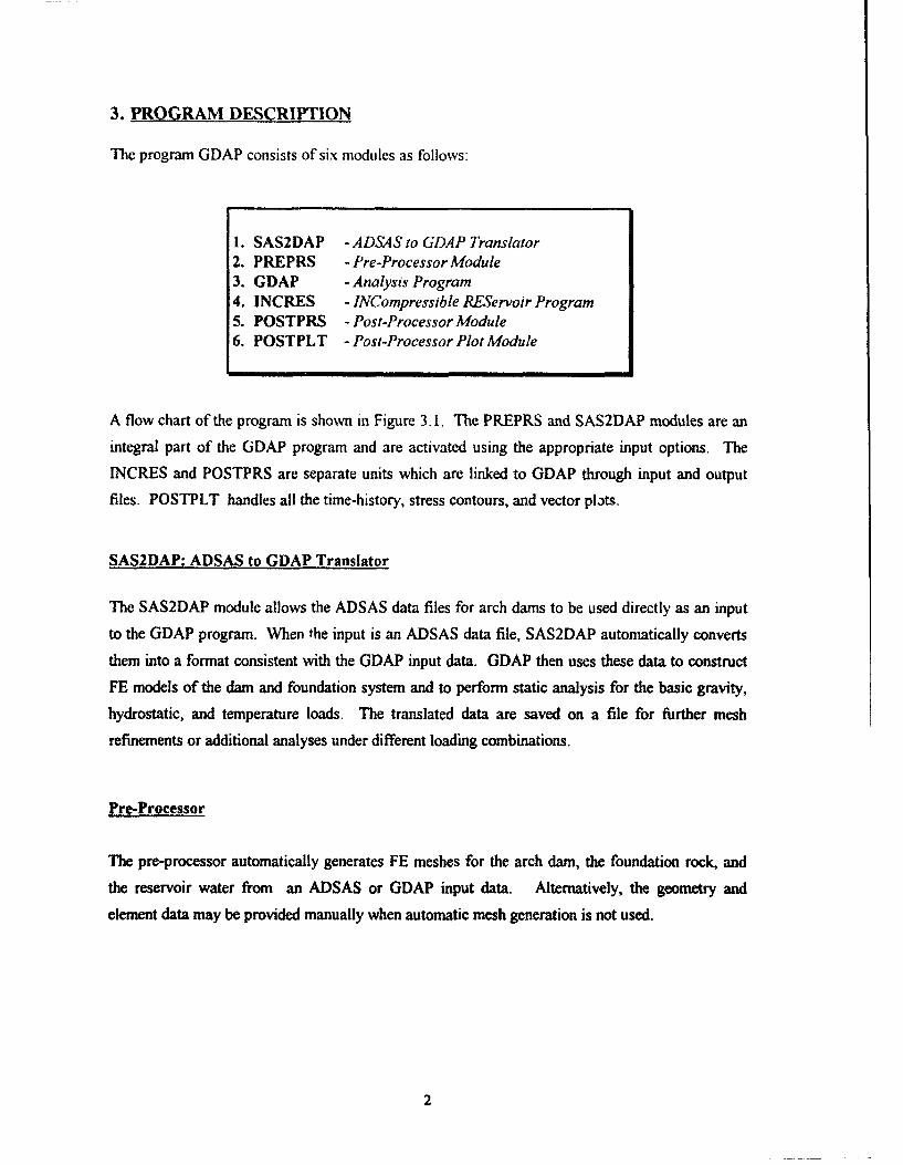
3. PROGRAM DESCRIPTION
The program GDAP consists of six modules as follows:
1. SAS2DAP - ADSAS to GDAP Translator2. PREPRS - Pre-Processor Module3. GDAP - Analysis Program4. INCRES - INCompressible REServoir Program5. POSTPRS - Post-Processor Module6. POSTPLT - Post-Processor Plot Module
A flow chart of the program is shown in Figure 3.1. The PREPRS and SAS2DAP modules are an
integral part of the GDAP program and are activated using the appropriate input options. The
INCRES and POSTPRS are separate units which are linked to GDAP through input and output
files. POSTPLT handles all the time-history, stress contours, and vector plats.
SAS2DAP: ADSAS to GDAP Translator
The SAS2DAP module allows the ADSAS data files for arch dams to be used directly as an input
to the GDAP program. When the input is an ADSAS data file, SAS2DAP automatically converts
them into a format consistent with the GDAP input data. GDAP then uses these data to constructFE models of the dam and foundation system and to perform static analysis for the basic gravity,
hydrostatic, and temperature loads. The translated data are saved on a file for further mesh
refinements or additional analyses under different loading combinations.
Pre-Processor
The pre-processor automatically generates FE meshes for the arch dam, the foundation rock, and
the reservoir water from an ADSAS or GDAP input data. Alternatively, the geometry andelement data may be provided manually when automatic mesh generation is not used.
2
Depending on the options selected, PREPRS will generate various 2-D and 3-D graphics that are
displayed on the computer monitor with the AutoCAD software package. AutoCAD is used also
for graphics editing, adding captions, cross-sectional hatching, combining various pictures, and
preparing hard copy plots for the report. The following is an outline of the various graphics that
can be generated by the pre-processor:
* 3-D plot of dam-foundation system* 3-D plot ofdam model alone* 3-D plot offoundation alone* 3-D plot of half of dam-foundation system* 3-D plot of reservoir model* 3-D shrink plots of dam, foundation, and reservoir* 3-D view of cantilever and foundation sections* Crown cantilever with line of centers* Plan view of arch or horizontal sections* Dam element numbers displayed on U/S and DiS faces0 Dam nodal numbers illustrated on both faces
In addition, the pre-processor has an option for automatic generation of an FE mesh for the
reservoir water. The reservoir model is assumed to be prismatic and extends upstream to a
distance equal to at least three times the water height, and it matches the concrete nodes at the
upstream face of the dam. The generated reservoir model is used as an input to the INCRES
program to calculate the incompressible added mass matrix or to plot a 3-D picture of the mesh.
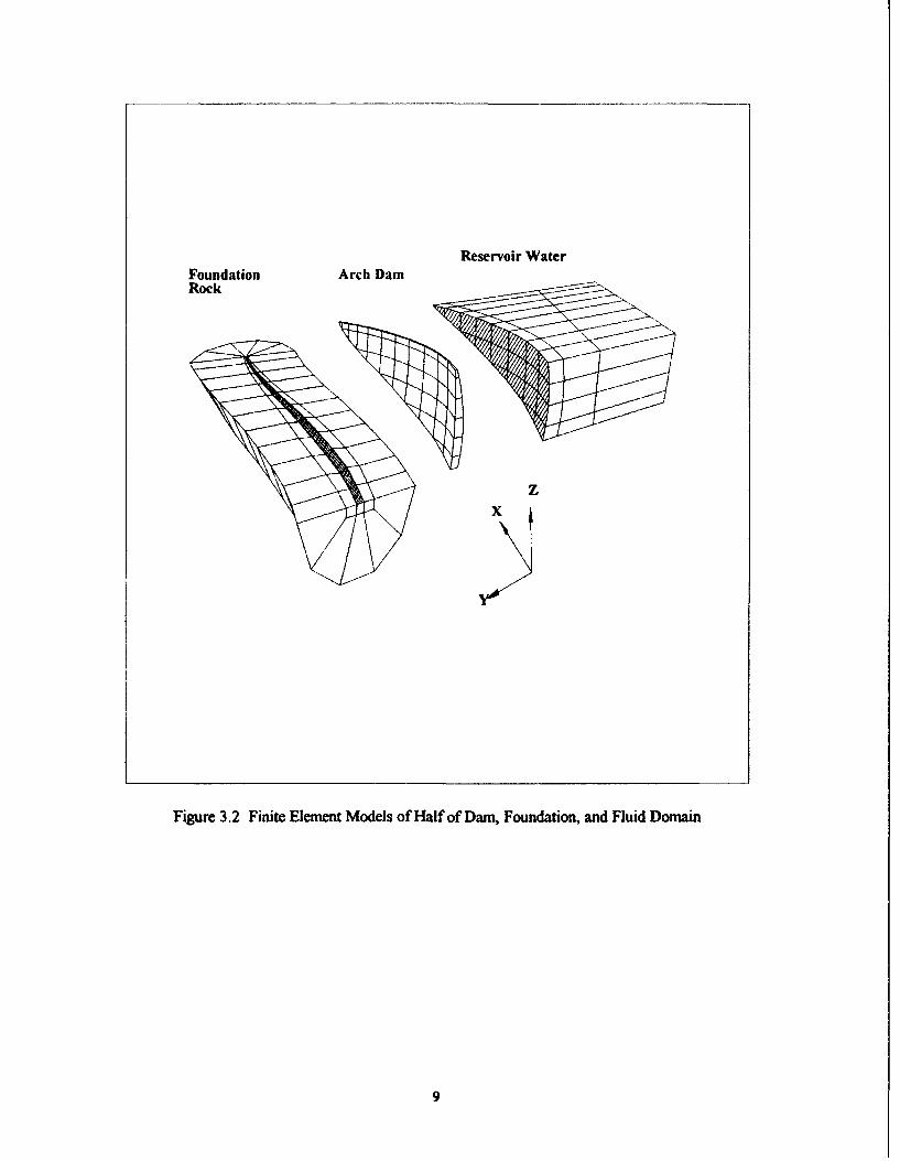
GDAP Program
GDAP is an FE program specifically designed for the static and dynamic analyses of concrete
dams. It includes an advanced mesh generator that automatically produces FE meshes for the dam,
foundation rock, and the reservoir water from a minimum amount of input information (Figure
3.2).
The static and dynamic analyses are based on the linear-elastic material properties. The static
loads include the separate or combined action of gravity, hydrostatic, temperature, silt, and the
concentrated loads; and the dynamic analysis includes both the response-spectrum and time-history
modal superposition methods.
3

Dam Model' GDAP makes two types of idealization for the automatic mesh generation of the
concrete arch as shown by Ghanaat and Clough.* The first idealization assumes one element
through the dam thickness and uses curved shell elements to model a thin arch dam. In the second
idealization, the concrete arch is idealized by three layers of eight-node, 3-D solid elements throt -
the dam thickness, which is more suitable for the gravity arch dams. Both element types are based
on isoparametric formulation and are described by Ghanaat *"
The extended mesh generator of GDAP can handle any general three-centered arch dam of
arbitrary geometry. The single- and two-centered arch dams are treated as special cases. The FE
mesh of the arch is first defined on the reference surface and then is projected onto the upstream
and downstream faces to get the nodal points. The reference surface is a vertical cylindrical
surface passing through the upstream edge of the crest In general, all nodes on the reference
surface are arranged on horizontal sections (called mesh elevations) and on vertical planes
projected from the intersection of mesh elevations with the dam-abutment interface. In addition.
the program permits to add free arch and cantilevers to the mesh layout at any prescribed elevation
to facilitate mesh generation of arch dams located in canyons with irregular and complex
geometry. A free cantilever is defined as a typical vertical line on the reference surface that is not
connected to a horizontal mesh line (mesh elevation) at its intersection with the abutment. This is
specially suitable for modeling arch dams in wide canyons (Figure 3.3). Similarly, a free arch is a
typical horizontal section on the reference surface that is not supported by cantilevers (or nor
connected to a vertical line) at its intersection with the abutment (Figure 3.4). The arches can be
free at one or both ends and the free cantilevers may be added at one or both abutments (Figure
3.5).
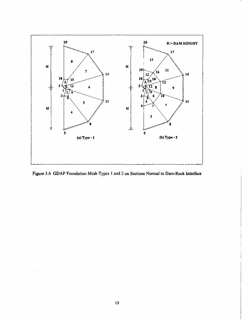
Foundation Model: The effects of foundation-dam interaction are accounted for by including an
appropriate portion of the foundation rock as part of the FE idealization. The GDAP mesh
generator module generates a prismatic foundation mesh and permits three degrees of refinements
based on the volume of rock and the number of ecr-Aits used in the foundation model.
The foundation mesh is constructed on semicircular planes cut into the canyon walls in the
direction normal to the dam-rock contact surface at the interface node locations (Figure 3.2). On
*Ghanaat, Y., and Clough, R. W. 1989. "EADAP: Enhanced Arch Dam Analysis Program", ReportNo. UCB/EERC-89/07, Earthquake Engineering Research Center, University of California, Berkeley,CA.**Ghanaat, Y. 1993. "Theoretical Manual for Analysis of Arch Dams" (Technical Report ITL-93-1),U. S. Army Engineer Waterways Experiment Station, Vicksburg, MS.
4
each of these planes, a semicircle is drawn from the dam-rock interface with a radius equal to the
dam height for the foundation mesh types one and two (Figure 3.6), and equal to two times of dam
height for the mesh type three (Figure 3.7). Three-dimensional, eight-node brick elements are used
for all three foundation mesh types. The number of foundation elements on each semicircular
plane for the three mesh types are 8, 13, and 18, respectively; the number of elements on each
plane are increased to 10, 15, and 20 when eight-node brick elements are also used to model the
concrete arch.
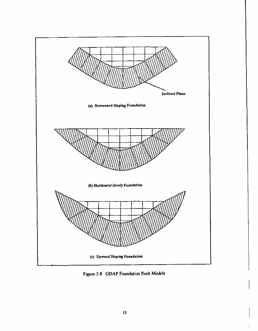
Furthermore, there are three options available for the orientation of the semicircular planes at the
crest level. These planes may have downward slopes (i.e. stay normal to the dam-rock contact
surface) or may be rotated upward to a horizontal or upward sloping position to represent the
actual canyon shapes (Figure 3.8).
INCRES Proeram
INCRES is an FE program for calculating an equivalent added mass matrix for the incompressiblereservoir water. The added mass of water is obtained from the hydrodynamic pressure
distributions on the face of the dam by solving the pressure wave equation. The calculated added-
mass matrix is then supplied as additional input data to GDAP to account for the dam-waterinteraction in the dynamic analysis.
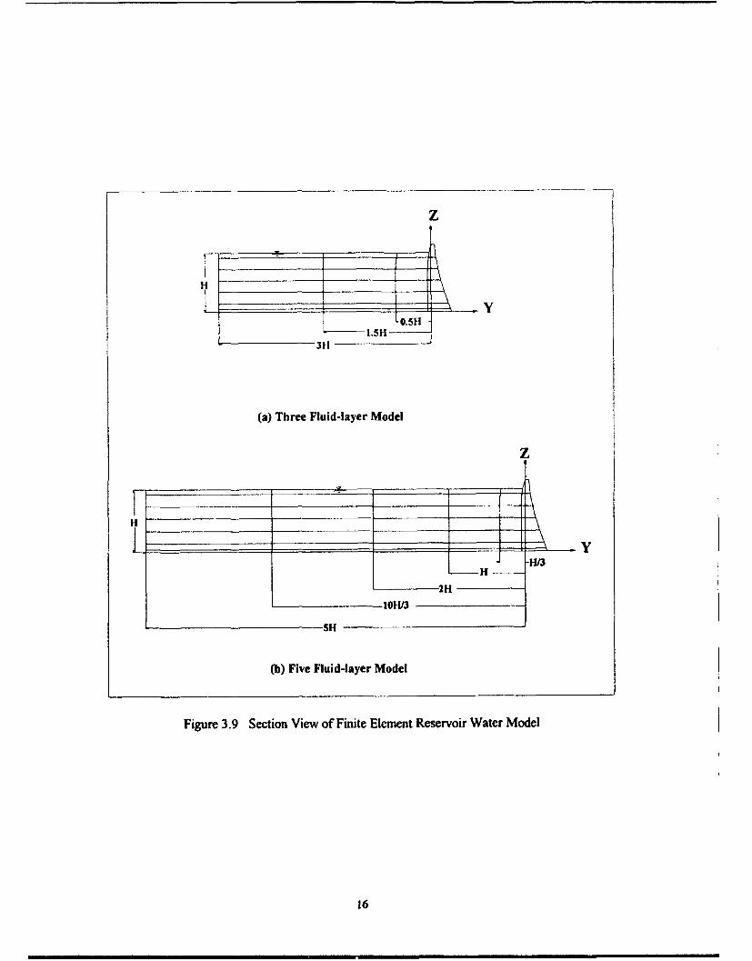
Reservoir Water Model: The GDAP pre-processor automatically generates a prismatic reservoir
FE model for calculating the added mass of the impounded water. The reservoir water model
consists of liquid elements arranged in three or more successive layers with liquid nodes located to
correspond with concrete nodes on the dam-reservoir interface. When the mesh generation
capability of GDAP is used, the reservoir water mesh extends upstream to a distance equal to the
number of fluid layers times the water depth. Figure 3.9 shows two prismatic reservoir models for
a three-layer and a five-layer liquid mesh. The dam-water interface is modeled by 8-node, 2-D
curvilinear elements, whereas the body of water is represented by 16-node, 3-D liquid elements
with nodal pressures being the unknowns. Both element types are based on the isoparametric
formulation and are described by Ghanaat." Topographic features of the reservoir may be
included in the FE model by manually modifying the generated nodal coordinates to match the
actual shape of the canyon.
* Op. cit. p.4.
5
Post-Processor
The GDAP post-processor (POSTPRS) converts the results of static and dynamic analyses into
appropriate plots and contours for easy review and evaluation.
POSTPRS reads the static deflections and vibration mode shapes calculated by GDAP and
generates the associated AutoCAD plot files. For the element stresses, however, the post-
processing is carried out in two steps. In the first step, POSTPRS reads the element stresses and
separates them into plot files including the upstream and downstream arch, cantilever, shear, and
principal stress components. In the second step, the stress plot files are used as input to the
POSTPLT plotting routine to generate stress contour plots of the arch and cantilever stresses,
vector plots of the principal stresses, or the time-history plots of the nodal displacements and the
element stresses.
Furthermore, the post-processor mcludes evaluation criteria for processing the large amount of
data produced in a typical response-history analysis. It automatically retrieves the envelope of the
maximum and minimum stress values that could occur at any instant of time, identifies all
significant concurrent stresses, recovers stress histories at all critical locations and at their
corresponding points on the opposite face of the dam, provides statistics regarding the number of
stress cycles exceeding the allowable stress (specified by the user), and calculates the excursion
time of stress cycles beyond the allowable values. A list of available features are summarized:
"* Plot of nodal displacements and mode shapes.
"• Contour plots of the arch and cantilever stresses due to the separate and combinedaction of various static loads.
"* Contour plots of the envelope arch and cantilever stresses due to the response spectrumdynamic analysis only and the response spectrum plus static loads.
"• Contour plots of the envelope arch and cantilever stresses due to the dynamic(response-history) only and the dynamic plus static loads.
"* Contour plots of concurrent stresses at critical instants of time due to the dynamic-only and the dynamic-plus static loads.
"* Vector plots of static, dynamic (response-history), and static-plus dynamic principalstresses.
" Time-history plots of the input earthquake motions and the critical nodal displacementsand element stresses.
6

* Statistics on number of stress cycles exceeding allowable stress and the correspondingexcursions of these stress cycles beyond specified limits.
POSTPLT
POSTPLT is an interactive plotting routine which runs under MS-DOS. The program prompts for
the input data and the names of the files containing the desired response quantities. The response
quantities include static or dynamic stress files or the nodal displacement and element stress
histories as generated by the post-processor. Stresses due to several load cases may be specified as
input. In that case, such stresses are combined and the desired plots are produced for the
combined action.
7

Mesh Manually CreatADSAS Generator F.E. Model
I ,Pre-Processor
SAutoCAD • ICE
XYZ3D ICE
INCRES V ANALYSIS
Post-Processor
AutoCAD POSTPLT
Figure 3.1 Flow Chart of GDAP Program
Reservoir Water
Foundation Arch DamRock
x
Figure 3.2 Finite Element Models of Half of Dam, Foundation, and Fluid Domain
9

(a) Without Free Cantilevers
(no a a--SI II
I II I
Free Cant-ilever- -(no arch at this elevation)
(b) With Free Cantilevers
Figure 3.3 Finite Element Mesh of an Arch Dam in Wide Canyon
10

(no cantilever at this elevatio
(a) Without Free Arches (b) With Free Arches
Figure 3.4 Finite Element of an Arch Dan in Narrow Canyon
11

(a) Without Free Archesand Cantilevers
Free Arch
Free Cant 'er Free Arch on One Side
(b) With Free Archesand Cantilevers
Figure 3.5 Finite Element of an Arch Dam in Irregular Canyon
12
20 20 H = DAM HEIGHT
17 17
413
H H
714 1912 1 11418 3 s18 3 510 12 12 6 2 1 2 9
3 3 6 1
Figure 3.6 GDAP Foundation Mesh Types I and 2 on Sections Normal to Dam-Rock Interface
13

26 H= DAM HEIGHT
7- 25
-H
-is
78 15 2
(€) Type - 3
Figure 3,7 GDAP Foundation Mesh Type 3 on Section Normal to Dam-Rock Interface
14
Inclined Plane
(a) Downward Sloping Foundation
(b) Horizontal (level) Foundation
(c) Upward Sloping Foundation
Figure 3.8 GDAP Foundation Rock Models
15
z
! - I
311
(a) Three Fluid-layer Model
Z
HH
EH LIM
2H1
1011/0
5H
(b) Five Fluid-layer Model
Figure 3.9 Section View of Finite Element Reservoir Water Model
16
4. Outi LINE OF STATIC ANALYSIS PROCEDURE
The GDAP program performs a linear-elastic static analysis of any arbitrary arch dam-foundation
system. The dam-foundation system is idealized as an assemblage of FE's as described in Section3. The geometric and element data are specified automatically by the mesh generation capabilities
or manually in accordance 1 the format description given in Section 6. Linear-elastic material
properties are assumed for i, the concrete and the foundation rock. Shell elements in the
concrete arch are assumed to be isotropic, but orthotropic properties may be assumed for the 8-
node solid elements representing the foundation rock. A detailed description of the static analysis
and the static loads is given by Ghanaat.°
The following static loads are considered and may be applied separately or in any arbitrary
combination:
* Gravity load* Water load* Temperature Load* Silt Load* Concentrated Load• Ice load
The results of static analysis include nodal displacements, element stresses, and the reaction forces
or thrusts at the dam-foundation interface due to the applied loads. For each thick-shell nodal
point, five displacement components corresponding to three translations and two rotations areprovided, whereas for all other nodal points only three translations are given. For each element, the
stresses are given at several points referred to as stress points. [Refer to Figures 6.9 and 6.10.1
All element stresses are calculated with respect to a set of local axes, except at the center of the 8-
node solid elements where they are given in reference to the global axes. The local stresses are
calculated on the upstream and downstream faces of the dam and include the arch, cantilever,
normal, shear, and the principal stresses. The reaction forces can be obtained at any nodal point,but they are normally needed at t6e dam-foundation interface for the stability analysis of the
abutment rock mass.
° Op. cit. p.4.
17
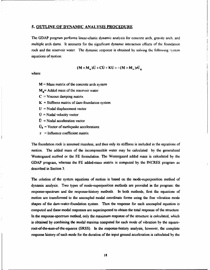
5. OUTLINE OF DYNAMIC ANALYSIS PROCEDURE
The GDAP program performs linear-elastic dynamic analysis for concrete arch, gravity arch, and
multiple arch dams. It accounts for the significant dynamic interaction effects of the foundation
rock and the reservoir water. The dynamic response is obtained by solving the following :ystem
equations of motion:
(M + M. )U +CUJ + KU =-(M + M,)rU,
where
M = Mass matrix of the concrete arch system
Ma= Added mass of the reservoir water
C = Viscous damping matrix
K = Stiffness matrix of dam-foundation system
U = Nodal displacement vector
UJ = Nodal velocity vector
0 = Nodal acceleration vector
Ug = Vector of earthquake accelerations
r = Influence coefficient matrix
The foundation rock is assumed massless, and thus only its stiffness is included in the equations of
motion. The added mass of the incompressible water may be calculated by the generalized
Westergaard method or the FE formulation. The Westergaard added mass is calculated by the
GDAP program, whereas the FE added-mass matrix is computed by the INCRES program as
described in Section 3.
The z;olution of the system equations of motion is based on the mode-superposition method of
dynamic analysis. Two types of mode-superposition methods are provided in the program: the
response-spectrum and the response-history methods. In both methods, first the equations of
motion are transformed to the uncoupled modal coordinate forms using the free vibration mode
shapes of the dam-water-foundation system. Then the response for each uncoupled equation is
computed and these modal responses are superimposed to obtain the total response of the structure,
In the response-spectrum method, only the maximum response of the structure is calculated, which
is obtained by combining the modal maxima computed for each mode of vibration by the square-
root-of-the-sum-of-the-squares (SRSS). In the response-history analysis, however, the complete
response history of each mode for the duration of the input ground acceleration is calculated by the
18
linear acceleration step-by-step integration method. The resulting modal displacements and stresses
at each time-step are then superimposed to obtain the total response history of the structure.
The earthquake response spectrum and the acceleration time-histories are used as seismic input for
the response spectrum and the response-history analyses, respectively. Any single component of
the selected seismic input or all three components may be applied in the dynamic analysis. The
results of analysis include the envelope nodal displacements and element stresses for the response
spectrum method and the time-histories of nodal displacements and element stresses for the
response-history analysis. In response-history analysis, the output also includes the maximum and
minimum response values and the associated time-steps.
19
6. GDAP INPUT DATA DESCRIPTION
The input data for the GDAP program and its pre-processor are prepared according to the free-
format specification given in this section. Each record contains one or several input values that are
separated by a comma or one or more contiguous blanks. The blanks are treated as separators,
thus the null values should be specified as zeros and not as blanks. The 1/0 system formats each
input value using the data type and the field width of the corresponding input list item.
GDAP INPUT DATA
A. TITLE RECORD
TITLE Information to be printed as the output header. Title is limited to 72 characters.
B. MASTER CONTROL PARAMETERS
One or both of the following records are required depending on the type of the input data.
Record B.1 - Model Definition and Analysis Type
This record is always required.
NUMNP Total number of nodal points in the dam-foundation model. Enter zero if MeshGeneration is used (Note-a).
MTOT Size of the available blank COMMON block (Note-b).
NELTYP Number of different element types to be used (Note-c).
LL Number of static load cases; enter zero in dynamic analysis.
NF Number of undamped natural frequencies to be calculated or number of modes tobe considered in the time-history or response-spectrum analysis. Enter zero forstatic analysis.
NDYN Analysis type selection:
Static Eigen Time Response GraphicsAnalysis Solution M Hstory Spectrum Pre-proesing
0 1 2 3 4
NLM Number of mesh elevations defining the dam model. Enter zero if mesh generationis not used.
NLU Mesh elevation number at the base elevation of a U-shaped valley (Figure 6.1).Enter zero for V-shaped valley.
20

NEQEST Estimated number of degrees of freedom (DOF's). Enter zero if no estimate isavailable. The execution halts if the estimated and computed DOF's do not match(Note-d).
IMODE Restart option for dynamic analysis:= 1, Mode shapes and frequencies are stored or read from the restart
TAPE O.DAT.= 0, otherwise and for static analysis.
IPRM Option for mode-shape printout in dynamic analysis:= 0, mode shapes are printed; = 1, otherwise.
ESTVOL Estimated total volume of all elements. Enter zero if no estimate of elementvolumes is available. The execution halts if estimated and computed volumes donot match with a 1OE-4 accuracy (Note-e).
MESH Dam mesh type:
= 0, manual data input, mesh generation is not used;= 1, dam is modeled by the combination of 16-node shell and thick-shell
elements, one element through the dam thickness is used;= 3, dam is modeled by 8-node brick elements, three elements through the
dam thickness are used.
MESHFN Foundation mesh type (Figures 3.6 and 3.7):
Rigid Type-I Type-2 Type-30 1 2 3
Enter zero when mesh generation is not used.
IADMAS Added-mass type selection for dynamic analysis:
Empty Reservoir Generalized Westergaard FEor Static Analysis Added mass Added mass0 1 2
For the FE option, a separate reservoir model should first be developed. Theadded mass is then obtained by running the INCRES program and is stored onTAPE12.DAT as an input for the GDAP dynamic analysis. When theWestergaard option is selected, the added mass is calculated by the GDAPprogram and no separate reservoir model is needed.
WATL Z-coordinate of the water level.
WDEN Water weight density.
21
Notes:
a) For THKSHEL elements only, the surface nodes are counted. When mesh generation isused, NUMNP is automatically calculated by the program and consists of the nodal pointsfor the dam with foundation mesh type-3.
b) MTOT controls the number of blocks and number of equations in each block for the out-of-core solution. Smaller MTOT values result in larger number of blocks with smallernumber of equations per block. Depending on the hardware resources, it could be set toany number in the range of 10,000-200,000.
c) Maximum of three element types can be specified: 8-node brick, element type-1; 16-nodeshell, element type-2; thick-shell, element type-3.
d) NEQEST may be used for checking the generated data. If set to a nonzero value otherthan the actual number of OOF's, nodal coordinates, ID array, and the element data aregenerated and then the execution stops.
e) ESTVOL may be used for further examination of the generated element data to identifyany excessive element distortions. If set to a nonzero value other than the actual totalvolume of all elements, stiffness and mass matrices for each element are calculated and theelements volumes and connectivities are printed out. Then the execution stops and noresponse is calculated.
22

\7
6
5
4
21
V-Shaped Dam (NLU 0)
NLM =7 - -
NLU=4
U-Shaped Dam (NLU - 4)
Figure 6.1 V-Shaped, U-Shaped Dams
Note: Dashed lines are fictitious grids used to construct FE mesh for the dam in a U-shaped valley. The base of the dam is located at elevation NLU.
23

Record B.2 - Dynamic Analysis with Restart Option
This record is required for dynamic response calculation for which mode shapes, frequencies, andelement data are read from the restart files. The first five parameters shown specify the problemsize and are retrieved from the output of the free vibration analysis. NFI and NF2 are the modeselection parameters. They allow inclusion of a single mode, a range of modes, or all thecalculated modes in the dynamic response calculation.
MBAND 1/2 bandwidth of the system of equilibrium equations-
NUMEL Total number of elements (dam plus foundation).
NEQ Number of equations or DOF's.
N3DDAM Number of 3-D brick elements in dam.
N3DFN Number of 3-D brick elements in foundation.
NSHEL2 Number of 3-D shell elements.
NSHEL3 Number of thick-shell elements.
NFI Starting mode number at which response calculation will begin,( 1 <NFI ___NF ).
NF2 Ending mode number at which response calculation will stop,(NF1 _<NF2•<NF).
24
C. MESH GENERATION INPUT DESCRIPTION
Skip this section if mesh generation is not used or if this is a dynamic response calculation forwhich the structural data and frequencies and mode shapes are read from the restart files.
Record C.1 - Reference Surface Data
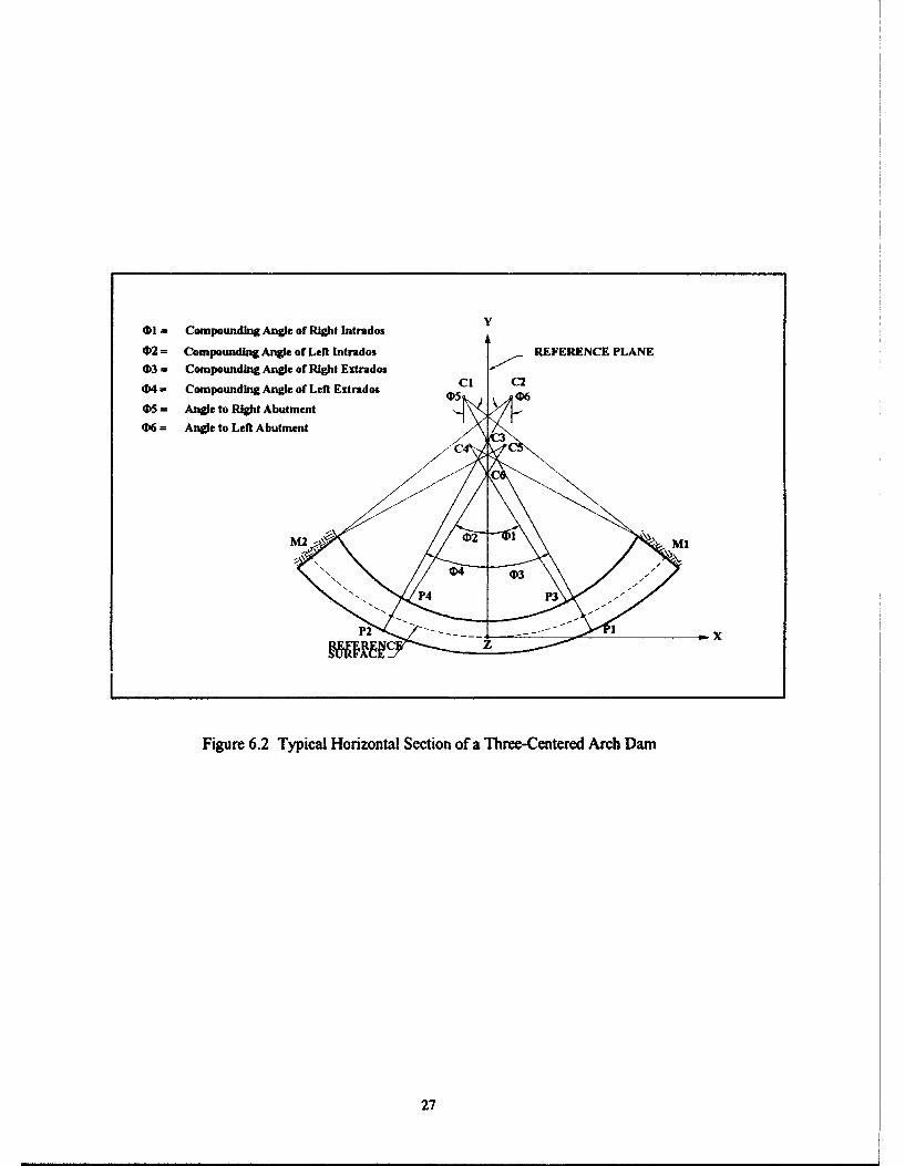
RI Radius of the inner portion of the reference surface* (Figure 6.2).
RO(1) Radius of the right outer portion of the reference surface.
RO(2) Radius of the left outer portion of the reference surface.
NL Number of design elevations.
IEL = 1, same compounding angles are specified at all elevations.
= 0, compounding angles differ for each elevation.
IRL = 1, same compounding angles are specified for the right and left portions of thedam.
= 0, otherwise.
liE = 1, same compounding angles are specified for intrados and extrados faces of thedam.
= 0, otherwise.
NRL = 1, same radius is specified for the right and left portions of intrados andextrados.
= 0, otherwise.
KFN Flag for orientation foundation planes at the top of dam:
= -I, standard downward inclined plane (Figure 3.8);
= 0, horizontal plane at the crest elevation;
= 1, upward inclined plane.
ISYM = 0, nonsymmetric dam, or when symmetry is not used.
= 1, symmetric dam modeled as a symmetric structure with symmetric boundaryconditions (BC's) along the crown section.
= -1, symmetric dam modeled as a symmetric structure with antisymmetric BC'salong the crown section.
Reference surface is a vertical cylindrical surface which passes through upstream edge of thecrest.
25

Record C.2 - Compoundin! Aneles and Angles to Abutments
One record is required for each design elevation to specify the compounding angles and angles toabutments (Figure 6.2). The sequence of records corresponds to increasing order of elevations.
EL(I) Elevation i.
FCI(I,1) Compounding angle of the right-intrados arc at elevation i, $•.
FCI(I,2) Compounding angle of the left-intrados arc at elevation i, $2.
FCE(I,1) Compounding angle of the right-extrados arc at elevation i, $3.
FCE(I,2) Compounding angle of the left-extrados arc at elevation i, $b.
FA(I,1) Angle to the right abutment at elevation i, *b.
FA(I,2) Angle to the left abutment at elevation i, 06.
Notes:
1. If IEL = 1 (Record C. 1), compounding angles for the first elevation only is required.
2. If IRL = I (Record C. 1), compounding angles for the right arcs only is required.
3. If lIE = 1 (Record C. 1), compounding angles of the intrados only is required.
Record C.3 - Temperature Data
Two sets of data records are required to specify the temperature data at the design elevations.
The first data set corresponds to the upstream face and as many records as required are supplied tospecify the temperature values at all design elevations. Temperature values are specified in thesequence of increasing elevations.
The second set of records corresponds to the downstream face. Temperature values are specifiedin exactly the same way as described above.
Zero values should be provided, if temperature variation is not considered in the analysis.
26
01 - Compounding Angle of Right Intrados
02 = Compounding Angle of Left Intrados REFERENCE PLANE
03 = Compounding Angle of Right ExtradosCI C2
04 = Compounding Angle of Left Extrados 05 06
05 = Angle to Right Abutment
06 = Angle to Left Abutment 7
C C
•.-, P4 P3 -
M z
Figure 6.2 Typical Horizontal Section of a Three-Centered Arch Dam
27

Record C.4 - Mesh Elevations
Mesh elevations are specified in increasing sequences, and as many records as required shouid besupplied. A maximum of 20 mesh elevations may be specified. The following data are suppliedfor each mesh elevation at which there is a supported or unsupported arch or cantilever line asshown in Figure 3.5.
ICNTRL(I,I) = 0, no arch line at mesh elevation i.= 1, an arch line is placed at elevation i.
ICNTRL(I,2) = 0, no cantilever line on the right side at this elevation.= 1, a cantilever line is placed on the right side at this elevation.
ICNTRL(I,3) = 0, no cantilever line on the left side at this elevation.= 1, a cantilever line is placed on the left side at this elevation.
ELM(I) Mesh elevation i.
Record C.5 - Intrados and Extrados Arcs
One record is required for each design elevation to specify the radius and Y-coordinate of thecenter of each arc (Figure 6.2). The sequence is according to the increasing order of the elevations.
YII Y-coordinate of center of intrados inner arc (point C6 in Figure 6.2).
YEI Y-coordinate of center of extrados inner arc (point C3).
RII Radius of intrados, inner arc.
REI Radius of extrados, inner arc.
RIO(l) Radius of intrados, right outer arc.
REO(1) Radius of extrados, right outer arc.
RIO(2) Radius of intrados, left outer arc.
REO(2) Radius of extrados, left outer arc.
Notes:
If NRL = I (Record C. 1), radii of the left outer arc for intrados and extrados may be set tozero.
28

Record C.6 - X-Coordinate of Center of Inner Arcs
Two set of records are required to specify the X-coordinate of the center of inner arcs at the designelevations.
The first set corresponds to the intrados inner arc. Coordinate values are specified in the sequenceof increasing elevations and as many records as required should be supplied.
The second set of records specify the X-coordinates of the center of the extrados inner arc. Sameprocedures mentioned above apply to this set.
Record C.7 - Material Properties of Elements
The following set of records specifies the material property identification numbers for each elementtype.
Record C. 7.1 - Eight-node Brick Elements of Dam
For mesh type-1 (MESH=I, Record B. 1), no record is required.
For mesh type-3 (MESH=3), when all eight-node brick elements of the dam have the same materialproperties (i.e. homogeneous concrete), two zeros, one for NLL and the other for MATT, asdescribed, should be supplied. In this case, material number I will be assigned to all eight-nodebrick elements of dam.
For mesh type-3, when eight-node brick elements of the dam have different material properties, onerecord should be assigned to each group of elements having the same material properties accordingto the following format:
NLL Element number.
MATT Material identification number.
Note:
The sequence of records should correspond with increasing order of the element numbers. If agroup of successive elements have the same material numbers, only material record for thefirst element in the group is needed. The sequence of records should be terminated by twozeros, unless the material number for the last element is supplied.
29
Record C 7 2 - Eight-node Brick Elements of Foundation
For the case with rigid foundation (MESHFN=O), no record is needed.
For MESHFN > 0 and both concrete arch dam and foundation rock are assumed to behomogeneous, two zeros should be supplied for NLL and MATT as described. In this case,material number I (if MESH = 1) or 2 (if MESH = 3) is assigned to eight-node brick elements ofthe foundation.
For MESHFN > 0 and either concrete arch dam or foundation rock is not homogeneous, a set ofrecords should be supplied to specify the material numbers of different foundation elements. Thesereco.'ds follow the same format described in Record C.7. 1.
Record C. 7.3 - 3-D Shell Elements
For the MESH not equal to 1, no record is required.
For MESH = 1 and all 3-D shell elements having the same material properties, NLL and MATTare set to zero; and the material number I is assumed for all 3-D shell elements.
For MESH = I and 3-D shell elements having different material properties, one record is suppliedfor each group of elements having identical material properties. These data are prepared accordingto the format described for Record C.7. 1.
Record C. 7.4 - Thick- Shell Elements
Follow the procedure presented for the 3-D shell elements.
30
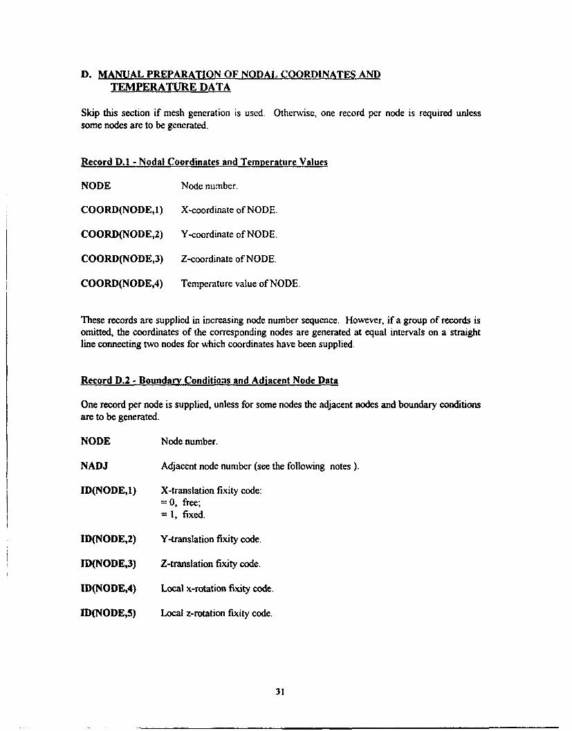
D. MANUAL PREPARATION OF NODAL COORDINATES ANDTEMPERATURE DATA
Skip this section if mesh generation is used. Otherwise, one record per node is required unlesssome nodes are to be generated.
Record D.1 - Nodal Coordinates and Temperature Values
NODE Node number.
COORD(NODEI) X-coordinate of NODE.
COORD(NODE,2) Y-coordinate of NODE.
COORD(NODE,3) Z-coordinate of NODE.
COORD(NODE,4) Temperature value of NODE.
These records are supplied in increasing node number sequence. However, if a group of records isomitted, the coordinates of the corresponding nodes are generated at equal intervals on a straightline connecting two nodes for which coordinates have been supplied.
Record D.2 - Boundary Conditioas and Adjacent Node Data
One record per node is supplied, unless for some nodes the adjacent nodes and boundary conditions
are to be generated.
NODE Node number.
NADJ Adjacent node number (see the following notes).
ID(NODE,1) X-translation fixity code:= 0, free;= 1, fixed.
ID(NODE,2) Y-translation fixity code.
ID(NODE,3) Z-translation fixity code.
ID(NODE,4) Local x-rotation fixity code.
ID(NODE,5) Local z-rotation fixity code.
31
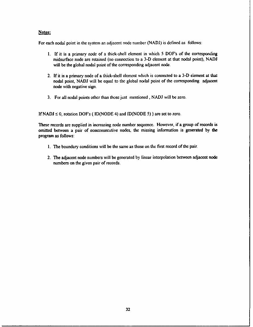
Notes:
For each nodal point in the system an adjacent node number (NADJ) is defined as follows:
I. If it is a primary node of a thick-shell element in which 5 DOF's of the correspondingmidsurface node are retained (no connection to a 3-D element at that nodal point), NADJwill be the global nodal point of the corresponding adjacent node.
2. If it is a primary node of a thick-shell element which is connected to a 3-D element at thatnodal point, NADJ will be equal to the global nodal point of the corresponding adjacentnode with negative sign.
3. For all nodal points other than those just mentioned , NADJ will be zero.
If NADJ < 0, rotation DOF's ( ID(NODE 4) and ID(NODE 5) ) are set to zero.
These records are supplied in increasing node number sequence. However, if a group of records isomitted between a pair of nonconsecutive nodes, the missing information is generated by theprogram as follows:
1. The boundary conditions will be the same as those on the first record of the pair.
2. The adjacent node numbers will be generated by linear interpolation between adjacent nodenumbers on the given pair of records.
32
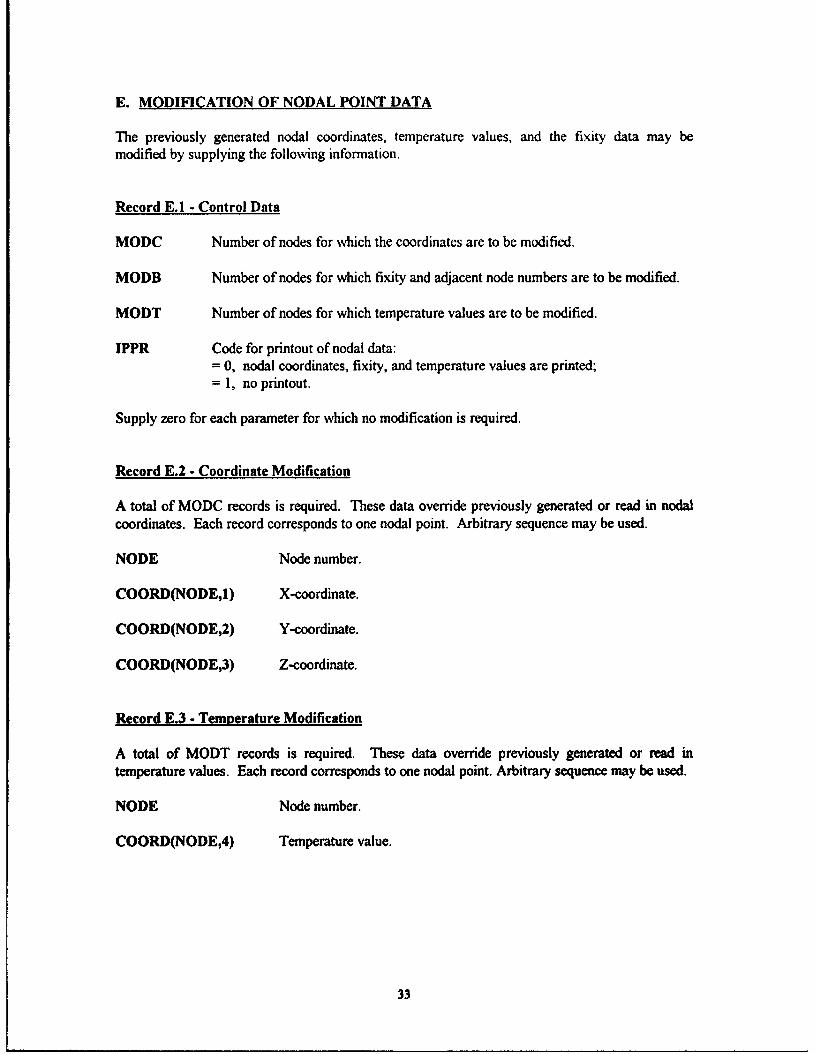
E. MODIFICATION OF NODAL POINT DATA
The previously generated nodal coordinates, temperature values, and the fixity data may bemodified by supplying the following information.
Record E.1 - Control Data
MODC Number of nodes for which the coordinates are to be modified.
MODB Number of nodes for which fixity and adjacent node numbers are to be modified.
MODT Number of nodes for which temperature values are to be modified.
IPPR Code for printout of nodal data:= 0, nodal coordinates, fixity, and temperature values are printed;= 1, no printout.
Supply zero for each parameter for which no modification is required.
Record E.2 - Coordinate Modification
A total of MODC records is required. These data override previously generated or read in nodalcoordinates. Each record corresponds to one nodal point. Arbitrary sequence may be used.
NODE Node number.
COORD(NODEI) X-coordinate.
COORD(NODE,2) Y-coordinate.
COORD(NODE,3) Z-coordinate.
Record E.3 - Temperature Modification
A total of MODT records is required. These data override previously generated or read intemperature values. Each record corresponds to one nodal point. Arbitrary sequence may be used.
NODE Node number.
COORD(NODE,4) Temperature value.
33
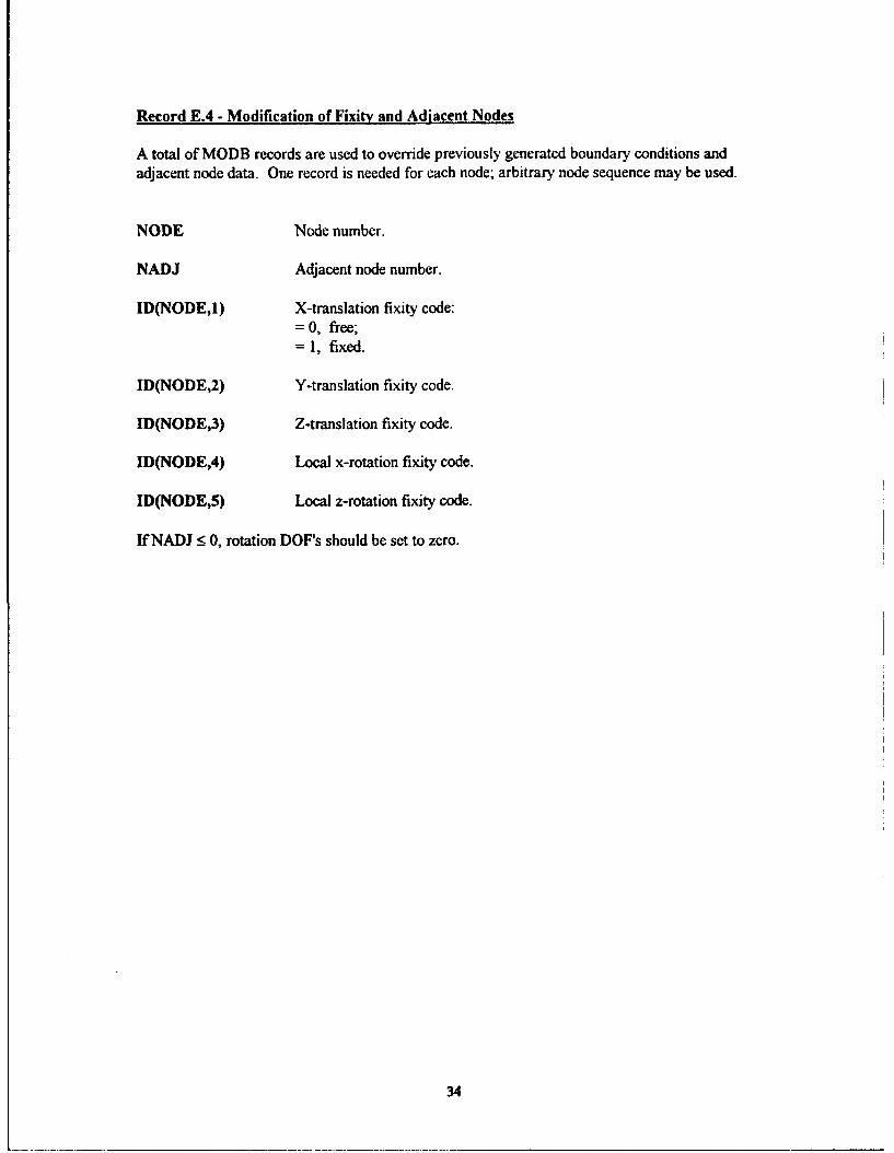
Record E.4 - Modification of Fixity and Adjacent Nodes
A total of MODB records are used to override previously generated boundary conditions andadjacent node data. One record is needed for each node; arbitrary node sequence may be used.
NODE Node number.
NADJ Adjacent node number.
ID(NODE,1) X-translation fixity code:= 0, free;= 1, fixed.
ID(NODE,2) Y-translation fixity code.
ID(NODE,3) Z-translation fixity code.
ID(NODE,4) Local x-rotation fixity code.
ID(NODE,5) Local z-rotation fixity code.
If NADJ < 0, rotation DOF's should be set to zero.
34

F. THICKNESS CHANGE
The program can handle a condition where thick-shell elements of different thicknesses areconnected, as shown in the drawing at the bottom of this page. In this case, the total nodes in thestructure include all surface nodes of thick-shell elements. The midsurface nodes of each pair ofelements along the thickness change are assumed to coincide at points marked by x in the drawing.In the input data, fixity condition and concentrated loads associated with primary nodes of one ofthe elements, say i, Q, and k, will refer to those of the midsurface. The primary nodes of the otherelements, 1, m, and n, will be fixed.
One record is required for each midsurface node along the thickness change. Fixed and free nodalpoints are selected so that J > I. This set of records must be terminated by a record with zeros forI and J.
I Corresponding fixed primary node.
J Corresponding free primary node.
\ k\n
/ k'
Connection of Thick-Shell Elements of Different Thicknesses
35

G. 3-D (8-NODE) BRICK ELEMENT DATA
This section is not required in dynamic analysis with restart option. Otherwise, the followingrecords are needed when 3-D (8-Node) brick elements are used in the FE model.
Record G.A - Control Data
MTYPE Element type number: enter 1 for 3-D (8-Node) brick elements.
NBRK8 Total number of 3-D (8-Node) brick elements. Enter zero if mesh generationis used.
NMAT Number of different material types.
NLD Number of different surface loads. Enter zero if mesh generation is used.
Record G.2 - Modulus of Elasticity and Poisson's Ratio
N Material identification number.
ISOT = 0, for isotropic material.= 1, for orthotropic material.
EE(1) Modulus of elasticity Exx.
EE(2) Modulus of elasticity Eyy.*
EE(3) Modulus of elasticity Ezz.*
EE(4) Poisson's ratio vxy.
EE(5) Poisson's ratio vyz.
EE(6) Poisson's ratio vzx
Enter zero for isotropic material.
36

Record G.3 - Shear Modulus and Thermal Coefficients
EE(7) Shear modulus G .xy
EE(8) Shear modulus G .*
EE(9) Shear modulus Gzx.
EE(10) Coefficient of thermal expansion ax
EE(I 1) Coefficient of thermal expansion ao.,
EE(12) Coefficient of thermal expansion ax .z
EE(13) Weight density of the material.
Record G.4 - Surface Loads
This record is not needed when mesh generation is used.
N Surface load identification number.
KTYPE Surface pressure type:= 1, uniform pressure;= 2, hydrostatic pressure.
PR Pressure value if KTYPE = 1.Weight density of water if KTYPE = 2.
ZREF Z-coordinate of the water level. Enter zero for KTYPE = 1.
NFACE Element face number upon which pressure acts (Figure 6.3).
Record G.5 - Reference Temperature and Gravity Acceleration
REFT Stress-free temperature.
GRAV Gravity acceleration.
Enter zero for isotropic material. It is set to Exx/2(1+vxy) by the program.
37

Record G.6- Element Data
This record set is not needed if mesh generation is used. 3-D brick elements are numbered from 1to NBRK8. One record is required for each element except for those that are to be generated.
NEL Element number.
NP(1) Node- I.
NP(8) Node - 8.
NINT Integration order.
MAT Material number.
INC Generation parameter.
MLD Surface pressure number.
ISP(I) Stress point number 1:Set to zero to calculate stresses at the center of the element.
ISP(2) Stress point number 2: Set to a prescribed element face number to calculatestresses at the center of that face. If zero, only stresses at ISP(1) are calculated.
38
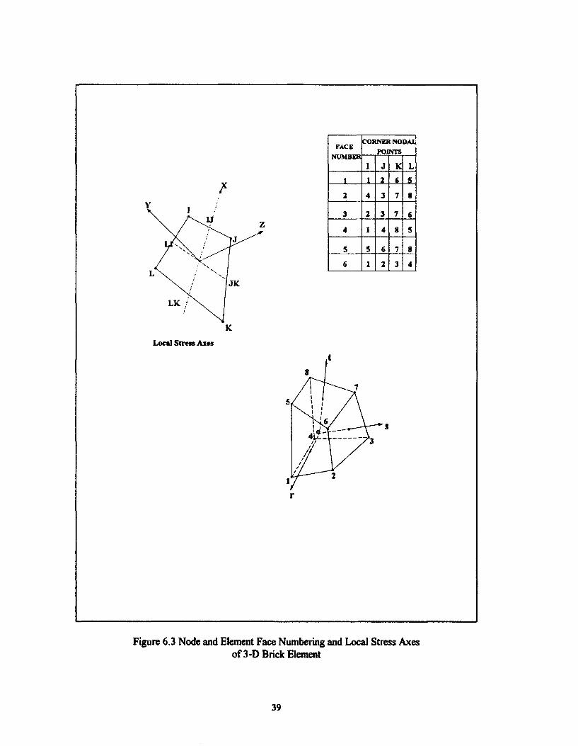
FA CORNER NODA4
NUMBER Pw
_ I_ I J K L
x 1 2 6 $1 2 4 3 7 8
3 2 3 7 6z I4 1 4 2 5
6 6 7 81, 6 1 12 3 4 1
/ JK
LK
K
Local Stress Axes
t
I 7
¢ '
/ 2
r
Figure 6.3 Node and Element Face Numbering and Local Stress Axesof 3-D Brick Element
39
H. 3D-SHELL ELEMENT DATA
Skip this section for a dynamic response calculation with the restart option. Otherwise, thefollowing records are supplied if 3-D shell elements are used in the FE model.
Record H.1 - Control Data
MTYPE Element type number: Enter 2 for 3-D shell.
N3DEL Total number of 3-D shell elements. Enter zero if mesh generation is used.
NMAT Number of material types.
NLD Number of surface load types. Enter zero if mesh generation is used.
Record H.2 - Material Properties
MAT Material identification number.
EE Modulus of elasticity.
ENU Poisson's ratio.
RHO Weight density of material.
ALPT Coefficient of thermal expansion.
Record H3 - Surface Loads
This record not needed when mesh generation is used.
N Surface pressure identification number.
KTYPE Surfiace pressure type:= 1, uniform pressure;= 2, hydrostatic pressure.
PR Pressure value if KTYPE = 1.Weight density of water if KTYPE = 2.
ZREF Z-coordinate of the water level. Enter zero if KTYPE = 1.
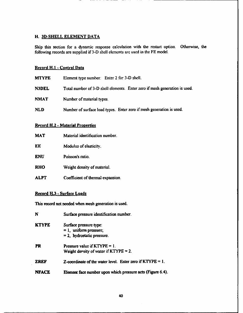
NFACE Element face number upon which pressure acts (Figure 6.4).
40
Record H.4 - Reference Temperature and Gravity Acceleration
REFT Stress free temperature.
GRAV Gravity acceleration.
Record H.5 - Element Data
Two records are required for each element except for those that are to be generated. Skip thisrecord set if mesh generation is used.
Record H. 5. 1
NEL Element number.
NINT Integration order: = 3, for regular shape; =4, for irregular shape.
MAT Material type number.
INC Generation increment.
MLD Surface pressure number.
IGG = 0, for 16-node elements.= 1, for 12-node degenerated elements.
Record H.5.2 - Element Connect:vity
NP(i) Element node numbers, i= 1, 2, ..., 16.
41

t
2
39
6 6
A C(b) 12-Node Degenerated 3-D She1 Elment
HulmRI 48~c
4!14 1248
2 2376
3 s562 14 873 4
[.5 1 2346 5673
(c) Element Face Numkeringe 3-D Shell Element
Figure 6.4 Element Node and Face Numbering of 3-D Sheli Element
42

I. THICK-SHELL ELEMENTS
Skip this section for a dynamic response analysis using the restart tapes. Otherwise, the followingdata records should be supplied if thick-shell elements are used in the FE model.
Record 1.1 - Control Data
MTYPE Element type number: enter 3 for thick-shell elements.
NUMEL Total number of thick-shell elements: Enter zero if mesh generation is used.
NMAT Number of material types.
NLD Number of surface load types: enter zero, it is set by the program.
Record 1.2 - Material Properties
MAT Material identification number.
EE Modulus of elasticity.
NU Poisson's ratio.
RO Mas density of the material.
GRAV Weight density of the material.
THERM Coefficient of thermal expansion.
Record 1.3 - Water and Temperature Data
ROWATER Weight density of water.
REFr Stress-free temperature.
43

Record 1.4 - Element Data
Skip this record set if mesh generation is used. Otherwise, for each element two records arerequired, and they are numbered in increasing sequence.
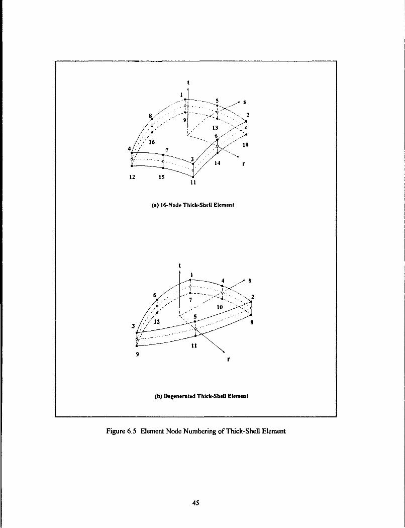
Record 14.1 Connectivity Data (Figure 6.5)
NN Element number.
IX(l) Node 1.
IX(8) Node 8.
Record 1. 4.2 -Material and Pressure Tvpes
MAT Material identification number.
PRESS(I) Uniform pressure (normal) acting on face t = -1.
PRESS(2) Uniform pressure (normal) acting on face t = +1.
44
t
13IV 6" /16 10
4 73
-14 r
12 15 11
(a) 16-Node Thick-Shell Element
t
I? "" I " 10',•
/12 \-"
11
9r
(b) Degenerated Thick-Shell Element
Figure 6.5 Element Node Numbering of Thick-Shell Element
45

J. PRE-PROCESSOR INPUT DATA DESCRIPTION
The input data for the graphics pre-processing are entered according to the specifications describedin this section. The following data are required when NDYN = 4 (Record B. 1).
Record J.l - Control Data
IPLOT =1, "Generates XYZ3-D plot files of the dam and foundation with hidden linesremoved. The following three files are generated:
File-name Descriptiondamfn.xyz Complete dam and foundation modelfn.xyz Foundation model alonehalfdfn.xyz Right-half portion of the dam and foundation model
Use these files as input to XYZ3-D to produce the desired 3-D pictures. The"p-7" optional parameter of the PICTURE directive of XYZ3-D n be setto 3 to save the final pictures in ASCII format. The "XYZ2-DXF"translator can then be used to convert these ASCII picture files into "DXF"format for interfacing with AutoCAD.
= 2, Generates AutoCAD 3-D and/or 2-D plot files (see Record J.4).
= 3, *Generates both the XYZ3-D and AutoCAD plot files.
IRES If not zero, a prismatic FE reservoir model consisting of IRES fluid layers isgenerated (Figures 3.9 and A. 13). The generated input data are stored in"incres.in" file which is used as input to the INCRES program for calculating theincompressible added mass.
Record J. 1. 1 - Shrink Plots
This record is needed for generating XYZ3-D shrink plots, when IPLOT = 1, or 3.
GAMA Shrinkage Factor: If zero, no shrink plot is generated. Otherwise, all dam andfoundation elements are shrunk by GAMA value (less than 1) to produce 3-Dshrink plots. For example, a GAMA of 0.2 will shrink each element by 20%. TheAutoCAD shrink file iq saved in "shrink.dxf," and the XYZ plot file is saved in"shrink.xyz" file which may be processed as described in Section J. 1.
* XYZ3-D provides 3-D plots with hidden lines removed. It is a good supplement to AutoCAD Release 9
and lower, which did not include advanced 3-D capabilities. If you have AutoCAD Release 10 andhigher, XYZ3-D is not required and you may use IPLOT = 2 only.
46

Record J.2 - 8-Node Elements
This record is needed when the mesh generation is not usd.,
N3DDAM Number of brick elements used in the dam.
N3DFN Number of brick elements used in the foundation.
Record J.3
This record is needed when IPLOT = I or 3, and the mesh generation is not used.
N3DDH Number of brick elements in the right-half portion of the dam.
N3DFH Number of brick elements in the right-half portion of the foundation.
NSHLH Number of 3-D shell elements in the right-half portion of the dam.
NTSHH Number of thick-shell elements in the right-half portion of the dam.
Record J.4 - Control Data For AutoCAD Plot Files
This record is needed when IPLOT = 2 or 3.
K3D If not zero, an AutoCAD plot file of the combined dam-foundation model isgenerated. In the generated AutoCAD "DXF" file, each element type is stored in aseparate layer as follows:
File name Layer No. Descriptionmesh3d.dxf I Foundation brick elements
2 Dam 3-D shell elements3 Darn thick-shell elements4 Dam brick elements
KUS If not zero, a plot of the U/S face of the dam projected on a vertical plane isgenerated. Element and node numbers are stored on separate AutoCAD layers foreasy inclusion or omission.
File name Layer name!us.d A( INODE NUMBERS, ELEMENT NUMBERS
KDS Same as KUS, except it is for the downstream face.
File name Layer nameds. Axf NODE NUMBERS, ELEMENT NUMBERS
47
KLOC If not zero, crown cantilever together with line of centers are generated and savedin "loc.dxrf file. Enter zero when mesh generation is not used.
KCANT If not zero, cantilever and foundation sections are saved in "cant.drf' file forplotting. In this case, KCANT is the number of cantilevers to be plotted. Thecantilevers for which plotting is requested are specified in Record J.5.
KARCH If not zero, arch sections at each mesh elevation are plotted. The file name for
arch sections is '"arch.dxj".
HT Height of a typical dam element. This is used to compute an appropriate text sizefor printing node and element numbers on the mesh plots. If set to zero, a faultvalue of 30.0 units consistent with the length units of the dam model will be used.
Record J.5 - Cantilever Sections
The following records are repeated KCANT times to specify all cantilever sections for whichplotting is required. Omit if KCANT = 0. Record J.5 is needed when mesh generation is used.Otherwise, the following two records should be submitted.
ICAN Cantilever number (See Figure 6.6).
ISIDE Side identification:= 1, right abutment;= 2, left abutment.
The following two Records (J.5.1 and J.5.2) are needed when mesh generation is not used.
Record J. 5.1
NEL Number of elements or polygons in the cantilever section.
Record J 5.2
This record specifies the element or polygon node numbers in a sequential manner. Repeat thisrecord for all NEL elements.
NNOD Number of element or polygon nodes.
IN(i) Element or polygon node numbers 1, 2, ..., NNOD.
48

CANTILEVER NUMBERS ([CAN)
1 2 3 4 5 6 7 8 7 6 5 4 3 21
LE"I ABUTMENT RIGHT ABUTMENTISIDE = 2 ISIDE =1
Figure 6.6 Cantilever Numbers
49

Record J.6 - Arch Sections
This record is needed when a plot of arch sections has been requested (i.e. KARCH is not zero),and the mesh generation is not used.
NELV Number of mesh elevations.
ELM(1) Mesh elevation at the base of the dam.
ELM(NELV) Mesh elevation at the crest.
Record J.7 - Reservoir Mesh
When IRES (see Record J.i) is not zero, records J.7.1 and J.7.2 are needed to generate an FEmesh for the reservoir. In addition, "fluid3d in", a preparatory fluid data file, should also beavailable (see Section 1-A of the Appendix).
Record J 7. 1
WATL Reservoir water level for added-mass calculation (i.e. Z-coordinate).
Z2 Z-coordinate of the upper edge of the dam elements that have their upper edgesjust above the water surface or coincide with the water surface.
ZO Z-coordinate of the midheight of the dam elements described above; enter zero, ifWATL=Z2.
Zi Z-coordinate of the lower edges of the corresponding dam elements; enter zero, ifWATL=Z2.
Record J. 7.2
The following records are needed when water surface does not coincide with a mesh elevationcontaining concrete element nodes. In that situation, the coordinates of the interface nodes at thewater surface and immediately below it should be provided.
NODE Node number.
X X-coordinate.
Y Y-coordinate.
Z Z-coordinate.
Provide as many records as necessary until all surface nodes and nodes immediately below themhave been specified.
50

K. STATIC ANALYSIS
The following records are required in static analysis only.
Record K.1 - Concentrated Nodal Loads
For each nodal point at which concentrated forces or moments are applied, a number of records arerequired. This number is equal to the number of load cases (LL in Record B. 1) in whichconcentrated loads are acting at that nodal point. The data records are provided according to thenodal number sequence and should be terminated by a record containing zero in each data field.Each record contains the following information:
N Node number.
L Load case number.
R(1) Force in X-direction.
R(2) Force in Y-direction.
R(3) Force in Z-direction.
R(4) Moment about local x-axis.
R(5) Moment about local z-axis.
Record K.2 - Reaction Force Control Data
Reaction forces (arch thrusts) at any desired interface nodes with the foundation rock (Figure 6.7),or at any desired contact nodes with a gravity thrust block (Figure 6.8) may be calculated byspecifying the following information.
NUMRE Number of reaction elements.
NUMRN Number of reaction nodes.
NUMRE and NUMRN should be set to zero, when computation of reaction forces are notrequired. In that case the following two records (K.2.1 and K.2.2) should be skipped.
51

Record K. 2.1 - Reaction Element Definition
IELEM(i) Reaction element numbers, i= 1,2,... NUMRE.
Record K 2.2 - Reaction Node Definition
INODE(i) Reaction node numbers, i= 1,2,...NUMRN.
Record K.3 - Element Loads
For each load case, one record is supplied to specify the element loads to be considered in theanalysis. Each load multiplier as defined below can be used to include or exclude any of the threebasic load types. A nonzero load multiplier can also be used to scale the corresponding load. Forexample, an AA = 1.2, which increases the gravity loads by 20%, is equivalent to increasing theunit weight of the concrete by 20%. This way the input data need not to be changed except for thisrecord. There are a total of LL load cases as specified in Section B. 1.
AA Gravity load multiplier:• 0, include gravity load and scale by AA;= 0, exclude gravity load.
BB Water load multiplier, same as AA.
CC Temperature load multiplier, same as AA.
52
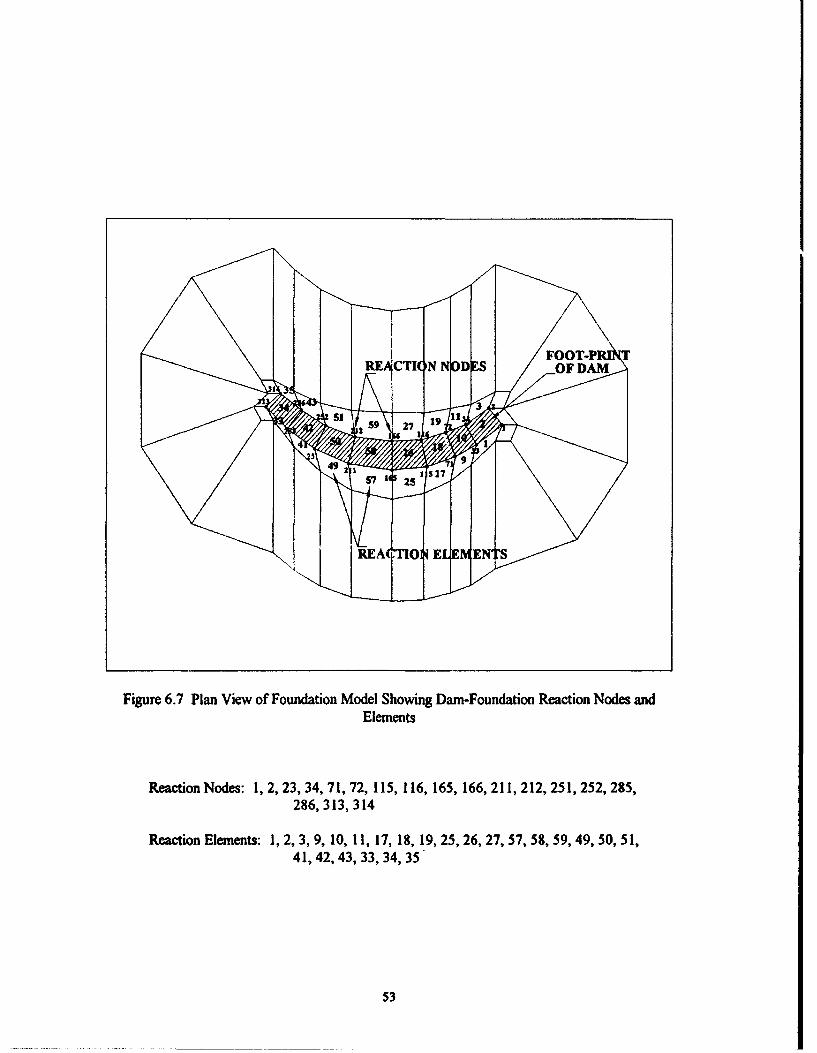
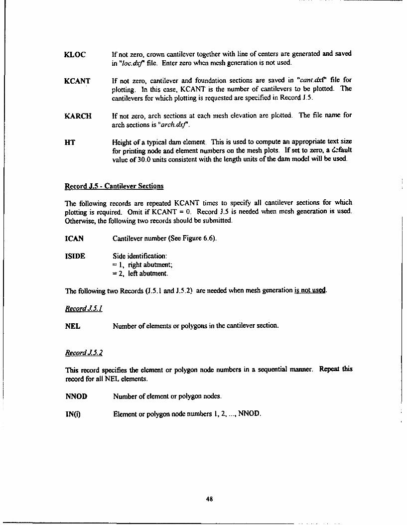
Figure 6.7 Plan View of Foundation Model Showing Dam-Foundation Reaction Nodes andElements
Reaction Nodes: 1, 2, 23, 34, 71, 72, 115, 116, 165, 166, 211, 212, 251,252, 285,286, 313, 314
Reaction Elements: 1, 2,3, 9, 10, 11, 17, 18, 19, 25, 26, 27, 57, 58, 59, 49, 50, 51,41, 42, 43, 33, 34, 35
53
ARCH DAM
REACTION
. •-....•: /ELEMENTS
GRAVITY BLOCK
Figure 6.8 Dam-Gravity Block Reaction Nodes and Elements
54

L. TIME-HISTORY ANALYSIS
The following records are needed in response-history analysis only.
Record L.A - Response Control Data
NFN Number of components of ground motion.
DT Integration time step. *
NT Total number of analysis time-steps.
NOT Time interval for printout of nodal displacements and stresses, expressed as amultiple of the integration time-step.
DAMP Modal damping ratio to be applied to all modes.
Record L.2 - Ground Motion Control Data
JFN(l) Identification number for the ground motion in the x-direction.
JFN(2) Identification number for the ground motion in the y-direction.
JFN(3) Identification number for the ground motion in the z-direction.
Record L.3 - Ground Motion
The following set of records is required for each component of the ground motion. The sequenceshould correspond to ground motion identification numbers and in increasing order.
Record L. 3.1 - Control Data
NLP Number of acceleration data points.
SFTR Scale factor multiplier (default = 1.0). It is also used to convert the inputaccelerations into appropriate units.
• The same integration time-step is specified for all modes. In general, a time-step at least 5 to 10 times
less than the lowest period of vibration will provide good accuracy for all modes that are considered in theanalysis. To assure numerical stability and accuracy of the solution, the GDAP program automaticallyfilters the high mode response, for which the period of vibration is less than 5 times the integration step.
55

Record L. 3.2 - Header
HED Title for the input motion.
Record L. 3.3 -Acceleration Data
T Time value at point 1.
P Acceleration value at point 1.
Four pairs of time and acceleration values are supplied in each record. As many records asrequired are provided to specify NLP pairs of data points.
Record LA - Dispacement Output
The following set of records is required to specify the displacement output results.
Record L. 4.1 - Control Data
KKK Code for output type:= 1, printout of displacement histories and maxima;= 2, plot of displacement histories and printout of maxima;= 3, printout of displacement maxima only.
ISP Plot spacing indicator.
Record L. 4.2 - Displacement Componenis
One record is required for each nodal point for which displacement plots or printout is requested.The set of records is in increasing order of nodal numbers. One record consisting of six zeros issupplied to terminate the sequence of records. Up to five displacement components may berequested for the thick-shell nodes and up to three components for all other nodes.
NP Node number.
IC Displacement component:= 1, X-component;= 2, Y-component;= 3, Z-component;= 4, local x-rotation;=5, local z-rotation.
56

Record L.5 - Stress Output
The following records are required to specify the stress output.
Record L.5.1 - Control Data
KKK Code for output type:= 1, printout of stress histories and maxima;= 2, plot of stress histories and printout of maxima;= 3, printout of stress maxima only.
ISP Plotting interval.
Record L. 5. 2 - Stress Components
For each element type used, a set of two records is required to specify the requested stresscomponents. The order of 3-D brick, 3-D shell, and thick shell should be followed. For eachelement, the first record contains desired element number (NEL) and its associated number ofstress components (NCOMP); and the second record specifies NCOMP requested stresscomponents. Each set is terminated by a record with two zeros for NEL and NCOMP asdescribed.
Record -1:
NEL Element number.
NCOMP Number of requested stress components.
Record -2:
This record contains the requested stress components of the element specified in Record-1. Up to12, 60, and 40 stress components may be requested for 3-D brick, 3-D shell, and thick-shellelements, respectively. The complete list of stress components for each element type issummarized in the following tables and also shown in Figures 6.9 and 6.10.
Although all stress components of all elements in the structure can be specified for output, onlyarch, cantilever, and the shear stresses in the surface direction are often used. Accordingly, theGDAP postprocessor only accepts arch, cantilever, and the surface shear stresses at each stresspoint. Therefore, for postprocessing purposes only these three stress components are consideredand are prescribed according to the following rules.
1. 8-node Solid: Stress components are specified only for the 8-node elements used in the dam.For each element two stress points, one at the center of one face and another at the centroid ofthe elements are specified (Table 6.1).
2. 3-D Shell: Specify arch, cantilever, and the surface shear stress components at all stresspoints and for all emcr, ts, except at the midedge locations common with the adjacent 3-Dshell elements (Table 6.2).
57
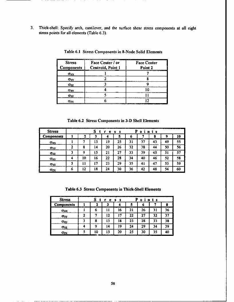
3. Thick-shell: Specify arch, cantilever, and the surface shear stress components at all eightstress points for all elements (Table 6.3).
Table 6.1 Stress Components in 8-Node Solid Elements
Stress F Face Center / or Face CenterComponents Centroid, Point I Point 2
Oxx 1 7_ _ _ 2 8
7ZZ 3 9axy 4 10avz 5 11
_ _zx 6 12
Table 6.2 Stress Components in 3-D Shell Elements
Stress S t r e s s P o i n t sComponents 1 2 3 4 5 6 7 8 9 10
Oxx 1 7 13 19 25 31 37 43 49 55aw 2 8 14 20 26 32 38 44 50 56077_ 3 9 15 21 27 33 39 45 51 57
Crxy 4 10 16 22 28 34 40 46 52 58o yz 5 11 17 23 29 35 41 47 53 59Uzx 6 12 18 24 30 36 42 48 54 60
Table 6.3 Stress Components in Thick-Shell Elements
Stress S t r e s s P o i n t sComponents 1 2 3 4 5 6 7 8
axx 1 6 11 16 21 26 31 36
oYY 2 7 12 17 22 27 32 37axy 3 8 13 18 23 28 33 38ayz 4 9 14 19 24 29 34 39CZX 5 10 15 20 25 30 35 40
58

s Z s
[3 r 4 r
7 8
x x
(a) Upstream Face (b) Downstream Face
Stress Point r s t I -Nd.,
1 +1 0 +1 12 92 +1 0 -1 16 123 -1 0 +1 10 84 -1 0 -1 1A4 - 115 0 +1 +1 9 76 0 +1 +1 13 107 0 -1 -1 11 NONE8 0 -1 +1 is NONE9 0 0 -1
10 0 0 +1
(c) Location of Stress Points
Figure 6.9 Stress Point Locations of 3-D Shell Element
59

z j z4e 30 7
r -, r
2e 6* e S
I-~ x x
(a) Upstream Face (b) Downstream Face
Stress Point r s t
1 -0.5774 -0.5774 o1
2 -0.5774 -0.5774 +1
3 -0.5774 +0.5774 -1
4 -0.5774 +0.5774 +1
5 +0.5774 -0.5774 -1
6 +0.5774 -0.5774 +1
7 +0.5774 +0.5774 -1
8 +0.5774 +0.5774 +1
(c) Location of Stress Points
Figure 6.10 Stress Point Locations of Thick-Shell Element
60

M. RESPONSE-SPECTRUM ANALYSIS
The following records are required only in response-spectrum analysis:
Record M.I - Control Data
MGM Number of components of the ground motion (1, 2, or 3).
IPD Code for displacement output:= 1, printout of modal and SRSS displacements are desired;= 0, no displacement printout.
IPS Code for stress output:= 0, compute stresses, print, and save SRSS stresses for plotting;= 1, do not compute stresses.
IPMOD Code for modal stress output (IPS = 0):= 0, no printout of modal stresses;= 1, print modal stresses for all elements.
Record M.2 - Acceleration-Snectrum Data
The following set of records should be supplied for each component of the ground motion (followthe X, Y, and Z order). If no ground motion is to be considered in a particular direction, tworecords with two zeros should be substituted instead.
Record M. 2.1 - Header Information
HED Title of ground motion.
Record M 2.2 - Control Data
NP Number of points specifying the acceleration spectrum.
SFTR Scale factor; use to scale spectral accelerations or to convert them intoconsistent units.
Record M 2.3 - Response-Spectrum Data
T Period value at point 1.
S Acceleration value at point 1.
One to four pairs of period and acceleration spectrum are specified in each record. Supply asmany records as required to define all NP points. Linear interpolation is used in the program tocalculate spectrum values for the periods between the specified input points.
61
7. INCRES INPUT DATA DESCRIPTION
The input data for calculating the FE added mass for the incompressible water is generated by theGDAP pre-processor according to the specifications described in this section. The pre-processorgenerates a standard prismatic reservoir water mesh extending upstream to a distance equal to thenumber of fluid layers multiplied by the water depth (IRES*WATL). The number of fluid layersIRES (Record J.l) is normally set to 3 or 5 as shown in Figures 3.9 and A.13. The liquid nodesare obtained by projecting the concrete nodes in the upstream direction. The reservoir boundariesand the upstream vertical plane are assumed to be rigid. For reservoirs with complicatedtopography, the standard mesh described above may not be adequate. In that case, the generatedinput data may be modified or the entire input data may be manually created to represent the actualtopography of the reservoir.
Record A - Title
This record contains information to be printed as the output header.
Record B - Control Data
NUMNP Total fluid nodal points.
NUMNS Number of fluid nodal points on the dam-reservoir interface.
N3DEL Number of 3-D fluid elements.
N2DEL Number of 2-D interface fluid elements.
WMASS Mass density of water.
GA Gravity acceleration.
WATL Z-coordinate of water level.ICOMP Comparison between the FE and Westergaard solution:
EQ. 0, no comparison is made; NE. 0, a comparison is made by subjecting thedam face to a pattern of unit g uniform accelerations in the ICOMP direction.(ICOMP= 1, 2, or 3 corresponding to the X, Y, and Z).
IPLOT Code for generation of plot files:= 0, do not generate plot file, solve for added mass;< 0, generate AutoCAD and XYZ3-D plots;> 0, generate AutoCAD plot only.
The comparison between the FE and the Westergaard method is made only for a simple pattern of unit gaccelerations that are applied in the global X, Y, or Z direction. This is essentially equivalent to a rigidbody motion of the dam, and thus flexibility of the arch structure is not considered. The resultinghydrodynamic pressures acting on the face of the dam and the equivalent nodal forces for each method areprinted out in the output file.
62
Record C - Nodal Coordinates
One record per nodal point is required to specify the coordinates and the boundary conditions. Thesequence of node numbering on each liquid section must follow the order in which the concretenodes on the interface have been numbered.
N Node number.
XYZ(1) X-coordinate.
XYZ(2) Y-coordinate.
XYZ(3) Z-coordinate.
IBC Boundary conditions:
EQ. 0, noninterface nodes below the water surface.EQ. 1, noninterface nodes at the water surface.EQ. -1, interface nodes below the water surface.EQ. -2, interface nodes at the water surface.
Record D - 2-D Element Data
One or both of the following records are required for each 2-D element on the interface. Thesequence of data is in increasing order of the absolute values of the element numbers.
D. I - Element Connectivit,
This record is always required. The element nodes must be input according to the order indicatedin Figure 7.1a.
NEL Element number:For an element that its nodes at the water surface do not coincide with thecorresponding concrete nodes, NEL is entered as a negative number.
NCON(1) Element nodal point i.*
NCON(8) Element nodal point 8.
NINT Integration order: 2 or 3 (2 is usually adequate).
Degenerated nodal points and the omitted midedge nodes should be set to zero. For example, theelement connectivity for the triangular 2-D element in Figure 7. la is 1, 2, 3, 0, 5, 6, 0, 8.
63

D. 2 - Z-coordinate of Surface Elements
This record is only required when NEL is negative. That is when the water surface level does notcoincide with the upper concrete element nodes.
Z2 Z-coordinate of the upper-edge nodes of concrete elements at the water surface.
ZO Z-coordinate of the midheight nodes of concrete elements at the water surface.
ZI Z-coordinate of the lower-edge nodes of concrete elements at the water surface.
Note:
Water level always lies between Z2 and Z 1.
Record E - 3-D Element Data
Two records are required for each 3-D fluid element. The sequence of records is in increasingorder of the element numbers.
E I - Element Identuiication
NE Element number.
NINT Integration order: 2 or 3 (usually 2 is sufficient).
E. 2 - Element Connectivit
The element nodes must be input according to the order indicated in Figure 7. lb.
NP(1) Element node number 1.-
NP(16) Element node number 16.
0 Degenerated nodal points and omitted midedge nodes should be set to zero. For example, elementnumbering of the triangular 3-D element in Figure 7. lb is 1, 2, 3, 0, 5, 6, 7, 0, 9, 10, 0, 12, 13, 14, 0, 16.
64
Record F - DOF's of Dam Interface Nodes
DOFs of dam nodes on the interface are entered according to the sequence of the reservoirinterface nodes (which by design follow the sequence of concrete nodes). DOF's of these nodesmay be obtained from the ID array of any previous GDAP analysis.
For each node only three translational DOF's are considered. Sixteen values per record areprovided, and as many records as needed are supplied to specify all DOF's of all interface nodes.
65
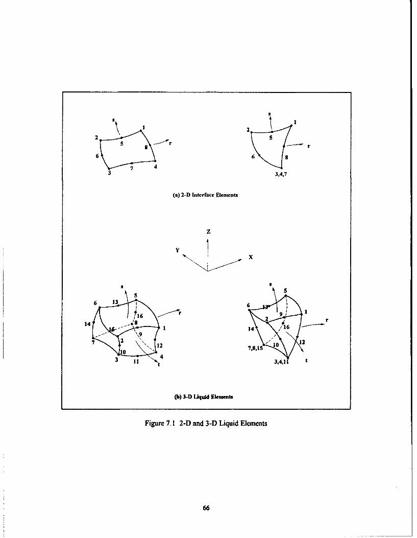
2
2 _ Sr
6 6
3 3,4,7
(a) 2-D Interface Elements
z
x
$ as5
6 13 6
916 12
414
3 3,4,11 t
(b) 3-D Uquid Elements
Figure 7.1 2-D and 3-D Liquid Elements
66

8. POST-PROCESSOR INPUT DATA DESCRIPTION
The GDAP post-processor is run after the completion of static or dynamic analysis. It reads filesgenerated by GDAP during the static and dynamic runs and produces appropriate plot files for theAutoCAD and POSTPLT graphics packages. The additional input data required for runningPOSTPRS is described in this section.
Record A - 8-Node Elements of the Dam
N3DDAM Number of 8-node elements used in the arch.
Record B - Control Data
LL Number of load cases in static analysis or number of mode-shapes to be plotted.Enter 1, for post-processing of the dynamic response.
KDISP Code for plot of static displacements. If not zero, displacement plots for LL staticload cases are generated and stored in file "disps.dxf'. Data for each load caseare stored in a separate AutoCAD layer; layer "LOAD-I" for load case 1, andlayer "LOAD-LL" for the load case LL. KDISP may be selected as a positive ornegative number to represent one of the following conditions.
KDISP > 0, displacements are plotted along horizontal arch sections only (SeeRecord F. 1 in this section).
KDISP < 0, displacements are plotted along any continuous section (RecordF.2).
KMODE Code for plot of mode-shapes. If not zero, LL mode-shapes are processed andstored in "modes.dxf'. Data for each mode is stored in a separate layer. Forexample layer "MODE-i" contains the mode i.
KMODE > 0, Mode-shapes are plotted along horizontal sections.KMODE < 0, Mode-shapes are plotted along nonhorizontal sections.
KSTAT Code for post-processing of static stresses. If not zero, stresses due to each loadcase are separated into the upstream and downstream components and are storedin separate files that are used as input to POSTPLT to prepare contour plots ofthe arch and cantilever stresses or vector plots of the principal stresses. Thedesignated names of the stress files are shown in the table in Appendix A, SectionD, POSTPLT Runs, bottom of p 78.
KRSPEC Code for post-processing of response-spectrum stresses. If not zero, SRSS stresscontour files for both faces of the dam are generated.
67

KTH Code for post-processing of time-history results. If not zero, time-history resultsare post-processed.
DSF Displacement scale factor (DSF); displacements are multiplied by DSF to convertinto desired units.
SSF Stress scale factor; stresses are divided by SSF to convert into desired units.
Record C - 3-D Brick Elements to be Excluded
This record set specifies 3-D brick elements which are to be excluded from the displacement orstress plots.
Static displacements and mode shapes are plotted for the upstream nodes of the dam face. It isassumed that there are three brick elements through the dam thickness. Consequently, those brickelements that are not part of the arch structure or the foundation rock (elements in the spillways orother structural features) should be excluded. Similarly, the stress plots are generated for theupstream and downstream faces of the dam, and thus brick elements that are not part of the archstructure are excluded.
Record C. 1 - Number of 3-D Brick Elements
NSI Number of brick elements to be excluded from the plots. Enter zero, if there arenone.
C. 2 - 3-D Brick Element Numbers
NELMI(i) Brick element numbers, i=I,2,...NS 1.
Record D - 3-D Shell Elements to be Excluded
This record set specifies the list of 3-D shell elements to be excluded from the displacement orstress plots. This includes all 3-D shell elements that are not part of the arch structure or do nothave common surface with the upstream face of the dam.
Record D. 1 - Number of 3-D Shell Elements
NS2 Number of 3-D shell elements to be excluded from the plots.
68
Record D. 2 - 3-D Shell Element Numbers
NELM2(i) 3-D shell element numbers, i = 1,2,...NS2.
Record E - Thick-shell Elements to be Excluded
This record specifies the list of those thick-shell elements that have no common surface with theupstream and downstream faces of the dam and should be excluded from the plots.
Record El - Number of Thick-shell Elements
NS3 Number of thick-shell elements to be excluded from the plots.
Record E.2 - Thick-shell Element Numbers
NELM3(i) Thick-shell element numbers, i = 1,2,...NS3
Record F - Mesh Elevations
This record is required when the plot of static displacements or dynamic mode shapes is requested.The deflections and mode shapes are plotted either along horizontal arch sections that are specifiedby their mesh elevations alone or along any continuous section which is specified by its nodalpoints and a representative elevation.
NELV Number of mesh elevations for which plot of displacements or mode-shapes arerequired.
PORD Maximum ordinate of displacement or mode-shape plots. When set to zero, avalue of 75 consistence with the length units of the model is assumed.
Record F I - Elevation of Horizontal Sections
This record is required when KDISP or KMODE > 0.
ELM(i) Mesh elevations, starting at the dam base, i = 1,2,...NELV.
Record F 2- Elevations and Nodal Points of Nonhorizontil Sections
These records are needed when KDISP or KMODE < 0. The following data should be specifiedfor each elevation for which plot of displacement or mode s'hape is requested.
69

ELM(i) Representative elevation i; base elevation is always entered first.
MD(i) Number of nodal points along elevation i.
NODID(j) Nodal points along elevation i, j=l,2,... MD(i).
Record G - Boundary Nodes
This record is needed when post-processing of static or response spectrum stresses is requested.Boundary nodes consist of the dam-foundation interface nodes and the nodes along the dam crest,and are used to define boundaries of the stress plots.
Record G. 1 - Number of Boundary Nodes
Only upstream nodes of the interface and the darn crest are required.
NU Number of boundary nodes.
Record G. 2 - List of Boundary Nodes
NUS(i) Boundary nodes, i = 1,2,...NU.
Record H - Post-processine of Time-History Results
Skip the following records if post-processing of time-history results is not desired (i.e. KTH = 0).
Record H. 1 - Control Data
KTHDSP If not zero, displacement histories are processed and stored in file "thdisp.plt"which will be used as input to POSTPLT.
KTHSTR If not zero, stress histories are processed and plot files are generated. For thename plot files (see table in Appendix A, Section D, POSTPLT Runs, bottom ofp 78).
KTHSTAT If not zero, static and dynamic stresses are combined and the post-processing isperformed for the combined stresses. If zero, dynamic stresses are not combinedwith the static stresses and all the subsequent post-processing are performed forthe dynamic stresses alone.
70

Record H. 2 - Tensile Strength of Concrete
TSTRNG Tensile strength or cracking strength of the concrete. This is used to identify alltensile stresses exceeding the cracking strength of the concrete.
Record H. 3 - File Name of Static Stresses
The following two records arn. required when KTHSTR is not zero. They contain the name of thestatic stress files that will be combined with time-history stresses or will be used to set up the stressplot files for the dynamic stresses alone.
Record I
USNAME Name of the file containing the upstream stresses for the desired static load case.Example: ustatl .str, ..., ustatLL.str, or any combination of these.
Record 2
DSNAME Corresponding name for the downstream stresses.
71

72
APPENDIX A
EXAMPLE DAM MODEL
73
ANALYSIS OF AN EXAMPLE DAM MODEL
An example dam-water-foundation model is developed to demonstrate the static and dynamicanalysis capabilities of the Arch Dam Analysis Workstation. A complete analysis includes modelgeneration using the GDAP pre-processor, static and dynamic response calculations, and post-processing of the analysis results.
The static analyses may be carried out for the separate or combined action of the various staticloads. If computed separately, not only the dam response for each individual load is available, butthey can also be combined by the post-processor to obtain the total response for various loadingcombinations. The dynamic analysis includes both response-spectrum and time-history modalsuperposition methods. The added mass of the incompressible water can be obtained by both thegeneralized Westergaard and the FE procedures.
The GDAP post-processor is used to present static deflections, vibration mode-shapes, stresscontours, and vector plots of principal stresses for the separate and combined static plus dynamicloads. In the time-history analysis, envelope and the critical concurrent sucssvs are automaticallyobtained by running the GDAP post-processor and are presented in the form of stress contours forboth faces of the dam. Vector plots of the principal stresses for the static plus time-history are alsoprovided. Furthermore, time-history of input ground accelerations; time-histories of critical nodaldisplacements; and time-histories of all stresses exceeding the cracking strength of the concrete arepresented.
The following six steps summarize analysis procedures for the example dam model. In each step,the input files, output files, and the associated programs are described. The input files in eachanalysis are specified by the user or obtained from the results of previous runs. The user-definedinput files are boldfaced.
74
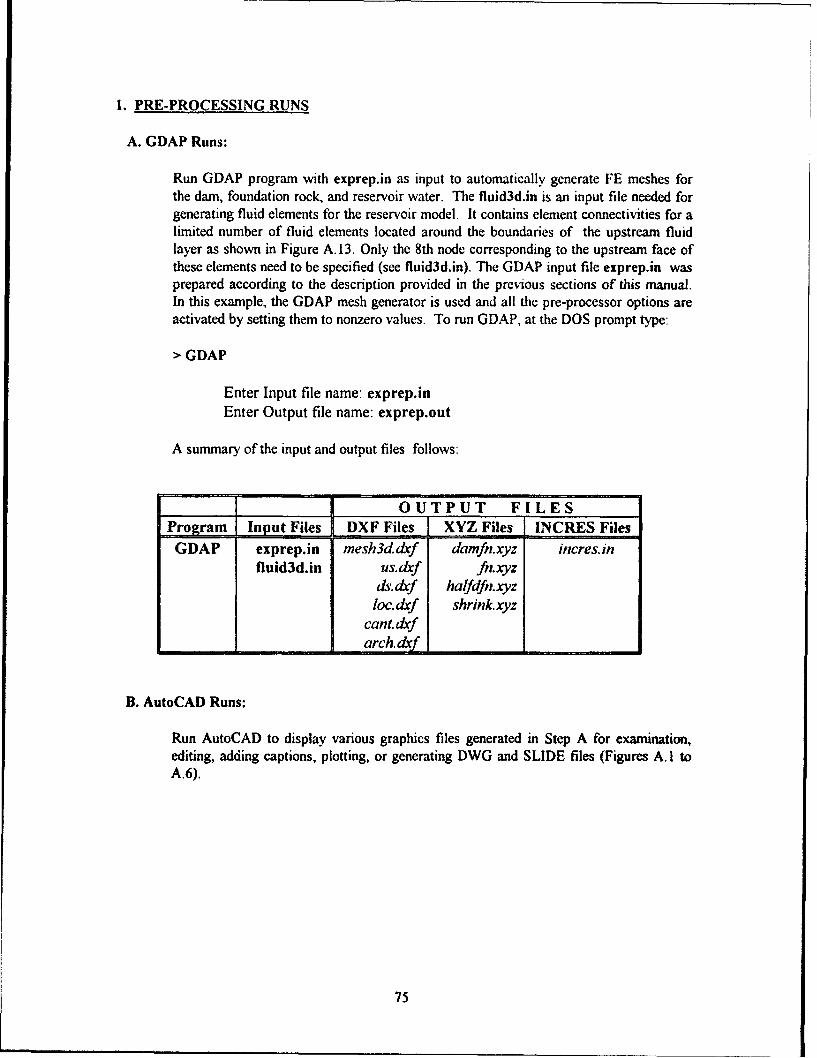
1. PRE-PROCESSING RUNS
A. GDAP Runs:
Run GDAP program with exprep.in as input to automatically generate FE meshes forthe dam, foundation rock, and reservoir water. The fluid3d.in is an input file needed forgenerating fluid elements for the reservoir model. It contains element connectivities for alimited number of fluid elements located around the boundaries of the upstream fluidlayer as shown in Figure A. 13. Only the 8th node corresponding to the upstream face ofthese elements need to be specified (see fluid3d.in). The GDAP input file exprep.An wasprepared according to the description provided in the previous sections of this manual.In this example, the GDAP mesh generator is used and all the pre-processor options areactivated by setting them to nonzero values. To run GDAP, at the DOS prompt type:
> GDAP
Enter Input file name: exprep.inEnter Output file name: exprep.out
A summary of the input and output files follows:
OUTPUT FILESProgram Input Files DXF Files XYZ Files INCRES Files
GDAP exprep.in mesh3d.dxf damfn.xyz incres.influid3d.in us. dxf fn.xyz
dsh df halfdfn.xyzloc.dxf shrink.xyz
cant. dxfarch. d _x
B. AutoCAD Runs:
Run AutoCAD to display various graphics files generated in Step A for examination,editing, adding captions, plotting, or generating DWG and SLIDE files (Figures A. I toA.6).
75

C. XYZ3D Runs (optional):
The last record of an XYZ input file includes the PICTURE directive or command forthe XYZ3D graphics package. The "P-7" parameter for the PICTURE directive isinitially set to I to draw and then save the generated picture on a binary file. TheXYZ3D prompts you for the name of this binary file. You may use the same input filename with extension ".plt" (see following output files table). If you wish to generate adifferent view of the picture, change the coordinate of the observer's position(OBSERVER directive) in the input file and rerun XYZ3D.
In addition, you can set "P-7" to 3 and rerun XYZ3D to save the generated picture inASCII format for interfacing with AutoCAD. When prompted for the name of thispicture file, enter the same input file name with extension ".pic".
OUTPUT FILESProgram Input Files [ (P-7 = 1) (P-7 = 3)
XYZ3D damfn.xyz damfn.plt damfn.picfn.xyz fn.plt fn.pic
halfdfn.xyz halfdfn.plt halfdfn.picshrink.xyz shrink.pit shrink.pic
D. XYZ2DXF Runs:
Run XYZ2DXF utility program to convert the ASCII picture files (with extension ".pic")generated in Step C to AutoCAD DXF files. The input and output files are specifiedinteractively. When prompted by XYZ2DXF, enter the name of input and output filesaccording to the following table:
Program Input Files DXF Files
XYZ2DXF damfn.pic damfn. dxffn.pic fn.dxf
halfdfa.pic halfdfn. dxfshrink.pic shrink. dxfl
Run AutoCAD to view the XYZ3D pictures that were just converted into DXF files(Figures A.7 to A.9).
Note that similar graphs (Figures A.7 to A.9) can now be generated using AutoCADRelease 10 or higher. For example, mesh3ddxf file and the AutoCAD "HIDE"command can be used to produce the hidden line graph shown in Figure A.7
76

2. STATIC ANALYSIS RUNS
A. GDAP Runs:
The input file for static run is exstat.in. This includes gravity and hydrostatic loads forthe full reservoir condition. Gravity and hydrostatic loads are designated as load cases Iand 2 and are applied separately Nodal displacements and element stresses for eachload case are calculated and stored in files "statdsp" and "statstr" for post-processing. Toperform static analysis, at the DOS prompt type the following:
> GDAP
Enter input file name: exstat.inEnter output file name: exstat.out
At the completion of static run, the following output files are generated.
Program Input Files I Output Files
GDAP exstat.in exstat. outtape l13.dattape8.datstrcoordstatdspstatstr
B. Post-processing Runs:
Run POSTPRS to generate plot files for the computed nodal displacements and elementstresses. The required input files for this run are shown in the following output filestable. The processed displacements and stresses are stored separately in two differentoutput files. The nodal displacements are saved in file "disps.dxf' where displacementsfor each load case are kept in separate AutoCAD LAYERs.
The static stresses for each load case are separated into the upstream and downstreamstresses and are saved in files with extension ".str". Each stress file name starts with theletter u or d to indicate upstream or downstream face and ends with a number to showthe load case. For example, ustat2, str indicates upstream static stresses for the load case2. Each stress file contains arch, cantilever, shear, and principal stresses as well as otherinformation needed to prepare stress contours and stress vector plots. To run POSTPRS,type the following:
> postprs
Enter input file name: poststat.in
Enter output file name: poststat.out
77

OUTPUT FILES
Program Input Files DXF Files POSTPLT Files
POSTPRS poststat.in disps. dxf ustatl.strtape l 3. dat dstat .strtape8. datstrcoord
statdsp ustaiLL. str
stalstr dstatLL. str
C. AutoCAD Run:
Run AutoCAD with "disps.dxf' as input to view the static deflections for each load case.The deflected shapes are drawn using the AutoCAD POLYLINE command. UseAutoCAD PEDIT command with spline curve-fitting option to smooth deflected shapes(Figure A. 10).
D. POSTPLT Runs:
Run the POSTPLT program to produce arch and cantilever stress contours, or togenerate DXF vector plot files for principal stresses for the separate or combined staticloads (1,2,...,LL load cases).
Program Input Files, Output
POSTPLT ustatl.str stress-contoursdstatl.str vector-plots
ustatLL.strdstatLL.str_
In this example the gravity and hydrostatic stresses were calculated separately, and werecombined during the post-processing. The stress contours for the combined loads areshown in Figures A. 11 and A.12a. POSTPLT stores the combined stresses in files"usta12.str" and "dstal2.str", with "12" indicating that load cases I and 2 are beingcombined. The vector plots of principal stresses for water load alone and for gravityplus water loads are given in Figures A. 12b to A. 12e.
7g

3. ADDED MASS OF RESERVOIR WATER
The added mass of incompressible reservoir water may be calculated using either the generalizedWestergaard method or the FE procedure. In the Westergaard method, the added mass of water iscalculated by simply setting IADMAS parameter to 1 (Record B. 1, Section 6.0, p 21); no reservoirmodeling is required. Whereas in the FE procedure, first an FE model of the reservoir water isdeveloped, and then the added mass is computed by using the INCRES program.
A. Pre-Processing Run:
Use the previously generated incres.in file as input, and run INCRES with a nonzeroIPLOT option (see the input description for INCRES, Section 7.0, p 62 of the main text)to generate a 3-D plot for the reservoir model. Depending on the IPLOT selected (RecordB, Section 7.0), DXF only or both XYZ and DXF drawings can be produced.
> incres
Enter input file name: incres.inEnter output file name: incres.out
Program Input Files Output Files
INCRES incres.in incres.xyzI I incres.dxrf
B. XYZ3D Runs:
Run XYZ3D to draw "incres.xyz", a 3-D picture of reservoir model with the hidden linesremoved. As discussed earlier in Step 1.C, p 76, "p-7" can be set to 1 or 3 to save theXYZ3D picture in a binary or ASCII format.
OUTPUT FILES
I Program I Input Files (p- 7 =) 1 (p-7 = 3) IXYZ3D : incres.xz incres.pit incres. ic
C. XYZ2DXF Run:
First run XYZ2DXF to translate "incres.pic" to an AutoCAD DXF file. Then executeAutoCAD to view reservoir model, to add captions, or to perform other tasks (FigureA.14).
I Program I Input Files DXF Files IXYZ2DXF incres.pic incres.dýr
79
D. FE Added-Mass Calculation:
Set the IPLOT option in "incres.in" to zero to compute the added mass of the reservoirwater. The output files for this run include the standard output file, incres.out, and abinary added-mass file, tape12.dai. This binary added-mass file will be used as an inputin the subsequent dynamic analyses.
> incres
Enter input file name: incres.inEnter output file name: incres.out
Programi Input Files Output Files
INCRES incres.in incres. out,tapel2.dat
80

4. FREQUENCY AND MODE-SHAPE RUNS
A. Flexible Foundation, Full Reservoir:
The lowest five vibration frequencies and mode shapes are calculated for the exampledam model. The input files for this run are the standard input file, exeigen.in, and theadded-mass file, tapel2.dat, produced by running INCRES. Note that tapel2.dat is notrequired when Westergaard method is used. The output files include the standard output,exeigen.out, and several restart tape files for the subsequent response analysis. Inaddition, mode shapes are stored in the binary file, modshap for post-processing.
> GDAPEnter input file name: exeigen.inEnter output file name: -xeigen.out
Program I Input Files I Output Files
GDAP exeigen.in exeigen. outtapel2.dat tape l3dat
tape IO.dattape9.dattape8.dattape l.datmodshap
B. Post-processing of Mode Shapes:
First run POSTPRS with posteigen.in as input to generate the AutoCAD DXF filemodes.dxf which contains the mode shapes. Each mode shape is stored in a separateAutoCAD LAYER called mode-], mode-2,... and so on. Now run AutoCAD to view themode-shapes, to add captions, or to perform other graphics tasks (Figures A. 15 to A. 19).Initially the deflected shapes are drawn as straight line segments by using the AutoCADPOLYLINE command, If smoothing is desired, use AutoCAD PEDIT command withspline curve-fitting option to smooth the mode-shapes.
> postprsEnter input file name: posteigen.inEnter output file name: posteigen.out
Program Input Files DXF Files
POSTPRS posteigen.in posteigen.outtape l13.dat modes.cxftape8. datmodshap
81

5. RESPONSE-SPECTRUM RUNS
A. Analysis Run:
The response-spectrum analysis is performed for three components of an exampleearthquake ground motion applied simultaneously in the stream, vertical, and cross-stream directions. The standard input file for this run is exrspec.in. It contains theearthquake response spectra shown in Figures A.20 and A.21 that were used as theseismic input. Other input files include the restart added-mass binary file, tapeI2.dat,and other files generated in the previous runs. Two output files are produced: thestandard output file exrspec.out, and file rmsstr which contains SRSS stress values forthe dam elements.
> GDAPEnter input file name: eirspec.inEnter output file name: exrspec.out
Program Input Files Output FilesGDAP exrspec.in exrspec. out
tape 12.dat rmsstrtape 10. dattape9.dattapeS.dattape J.dat
B. Post-processing Run:
Run POSTPRS with the input files specified in the following table to generate stresscontour plot files. Uspecl.str and dspecl.str are stress files for the upstream anddownstream faces of the dam which could be plotted separately or combined with thestatic stresses (see Step C , POSTPLT runs on following page).
> postprsEnter input file name: postspec.inEnter output file name: postspec.out
Program Input Files POSTPLT Files
POSTPRS postspec.in postspec. outtape 13.dat uspecl.strtapeS, dat dspecl.strsircoord
rmisstr
82

C. POSTPLT Runs:
Run POSTPLT to produce contour plots for the arch and cantilever stresses. The stresscontours can be drawn for the response spectrum alone or for the response-spectrum plusstatic stresses due to various static loading combinations computed previously.
> postplt
P ram Input Files Outut
POSTPLT uspecl.str contour plotsdspecl.str I
The contour plots of the envelope arch and cantilever seismic stresses computed based onthe Westergaard added mass are shown in Figures A.22b and A.23b.
The seismic stress contours computed using the FE added mass are shown in FiguresA.22a and A.23a. The total stresses for the combined seismic plus static loads(ustal2.str and dstal2.str) are presented in Figures A.24 and A.25.
83

6. TIME-HISTORY RUNS
A. GDAP Run:
Time-history analysis of the darn model is performed for three components of a specifiedearthquake ground motion shown in Figures A.26 to A.28. The ground acceleration time-histories are applied simultaneously in the stream, vertical, and cross-stream directions. Theinput files include the standard input exthist.in and the same restart binary files used in theresponse-spectrum analysis The output files are the standard output file, exthist.out, andseveral binary files containing the nodal displacements and element stresses.
> GDAP
Enter input file name: exthist.inEnter output file name: exthist.out
Program Input Files Output FilesGDAP exthist.in exthist.out ; standard output
tape 12.dat thdispl ; maximum nodal displacementstapelO.dat thdisp2 ; time-histories of selected nodal
displacements
tape9. dat thstrl ; maximum arch, cantilever, and shear stressestape8.dat ihstr2; time-histories of selected element stressestape l.dat thstprl; maximum and minimum principal stresses
I thstpr2 ; time-histories of selected principal stresses
B. Post-processing Run:
The input files for post-processing of the time-history results consist of postth.in constructedaccording to the description of input data for POSTPRS program and the previously generateddisplacement and stress time-history files. In addition, when static plus dynamic stresses arerequired, the desired static stresses are also provided as input. These are the upstream anddownstream stresses for a particular loading combination that have been generated in aprevious static analysis.
The output files include the envelope tensile and compressive stresses, concurrent stresses atcritical time-steps, and time-history of critical stresses and displacements. These files arelisted in the following table and are described in Step C, POSTPLT runs on the followingpage.
> postprsEnter input file name: postth.inEnter output file name: postth.out
84
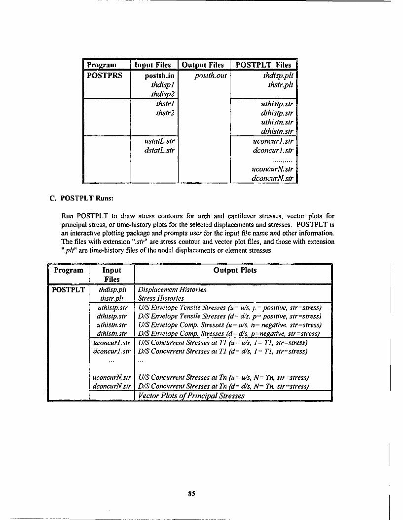
Program Input Files [Output Files ] POSTPLT Files
POSTPRS postth.in postth.out thdisp.pltthdispI thsir.plt
. thdisp2thstrl uthistp. sirthstr2 dthistp.str
uthistn. sirdthisin. str
ustaiL. str uconcurl. strdstatL.str dconcurl.str
uconcurN.sirdconcurN str
C. POSTPLT Runs:
Run POSTPLT to draw stress contours for arch and cantilever stresses, vector plots forprincipal stress, or time-history plots for the selected displacements and stresses. POSTPLT isan interactive plotting package and prompts user for the input fiDe name and other information.The files with extension ".str" are stress contour and vector plot files, and those with extension".pit" are time-history files of the nodal displacements or element stresses.
Program Input Output PlotsFiles
POSTPLT thdisp.plt Displacement Historiesthstr.plt Stress Histories
uthistp.str U/S Envelope Tensile Stresses (u = u/s, -, = positive, str=stress)dthistp.str D/S Envelope Tensile Stresses (d= d/s, p= positive, str=stress)uthistn.str U'S Envelope Comp. Stresses (u= u/s, n= negative, str=stress)dthistn.str D/S Envelope Comp. Stresses (dd= dis, p =negative, str=stress)
uconcurl.str U/S Concurrent Stresses at TI (u = u/s, I = T1, str=stress)dconcurl.str DIS Concurrent Stresses at Ti (d= d/s, I = TI, str=stress)
uconcurN.str U/S Concurrent Stresses at Tn (u= u/s, N= Tn, str=stress)dconcurN.str DIS Concurrent Stresses at Tn (d= d/s, N= Tn, str=stress)
Vector Plots of Principal Stresses
85
In this example only the combined static plus dynamic stresses are presented. The crackingstrength of the concrete is arbitrarily set to 350 psi (2.41 megapascals). The contours of theeavelope tensile stresses are displayed in Figures A.29 and A.30. All critical stressesexceeding the cracking strength of the concrete arc cantilever type. There are three criticaltime-steps corresponding to the maximum cantilever stresses. The contours of concurrentstresses at two critical time-steps are presented in Figures A.31 and A.32. The vector plots ofenvelope principal stresses are shown in Figures A.32b and A.32c. Time-history of nodaldisplacements for two selected nodes are shown in Figure A.33. Time-histories of all stressesexceeding the cracking strength of the concrete are displayed in Figures A.35 to A.38. In eachfigure, two stress histories are shown; one for a point with the maximum stress and the otherfor its pair on the opposite face of the dam.
86
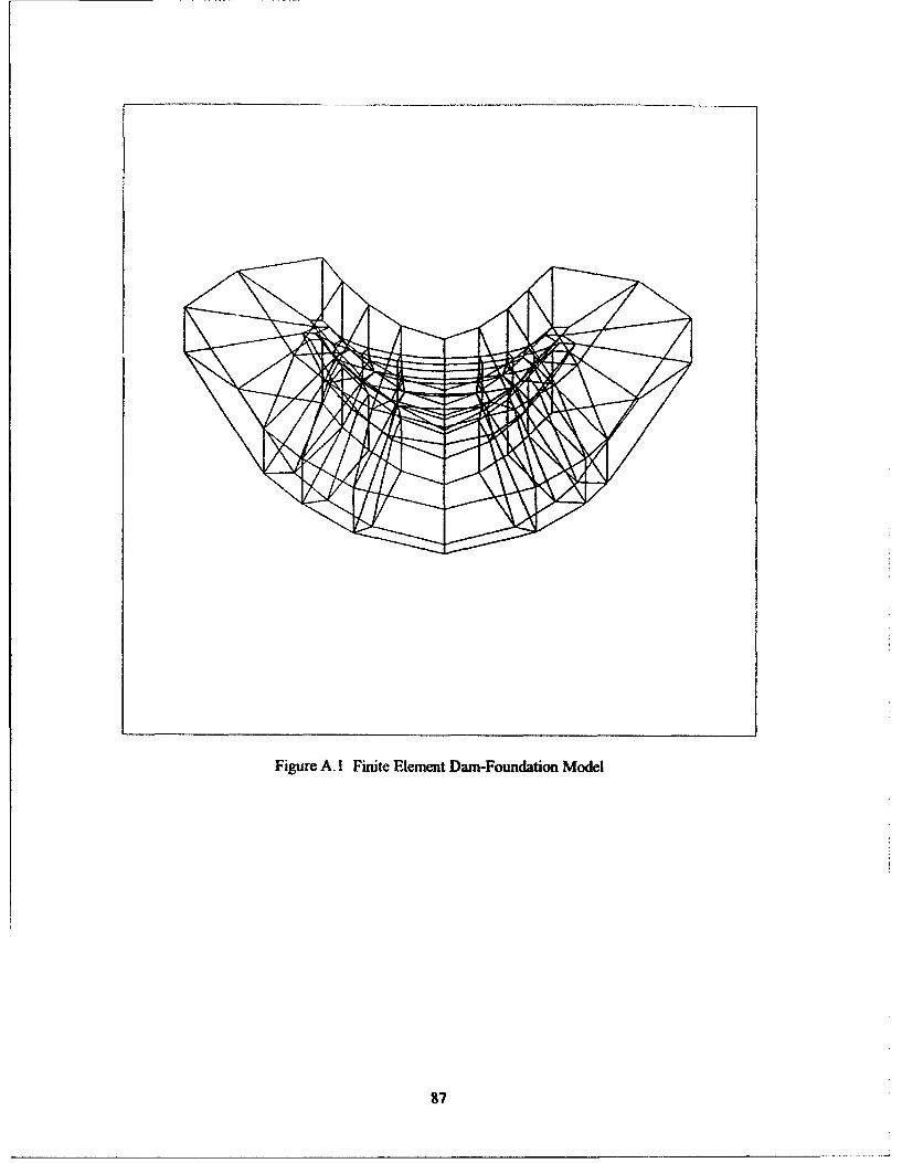
Figure A. I Finite Element Dam-Foundation Model
87
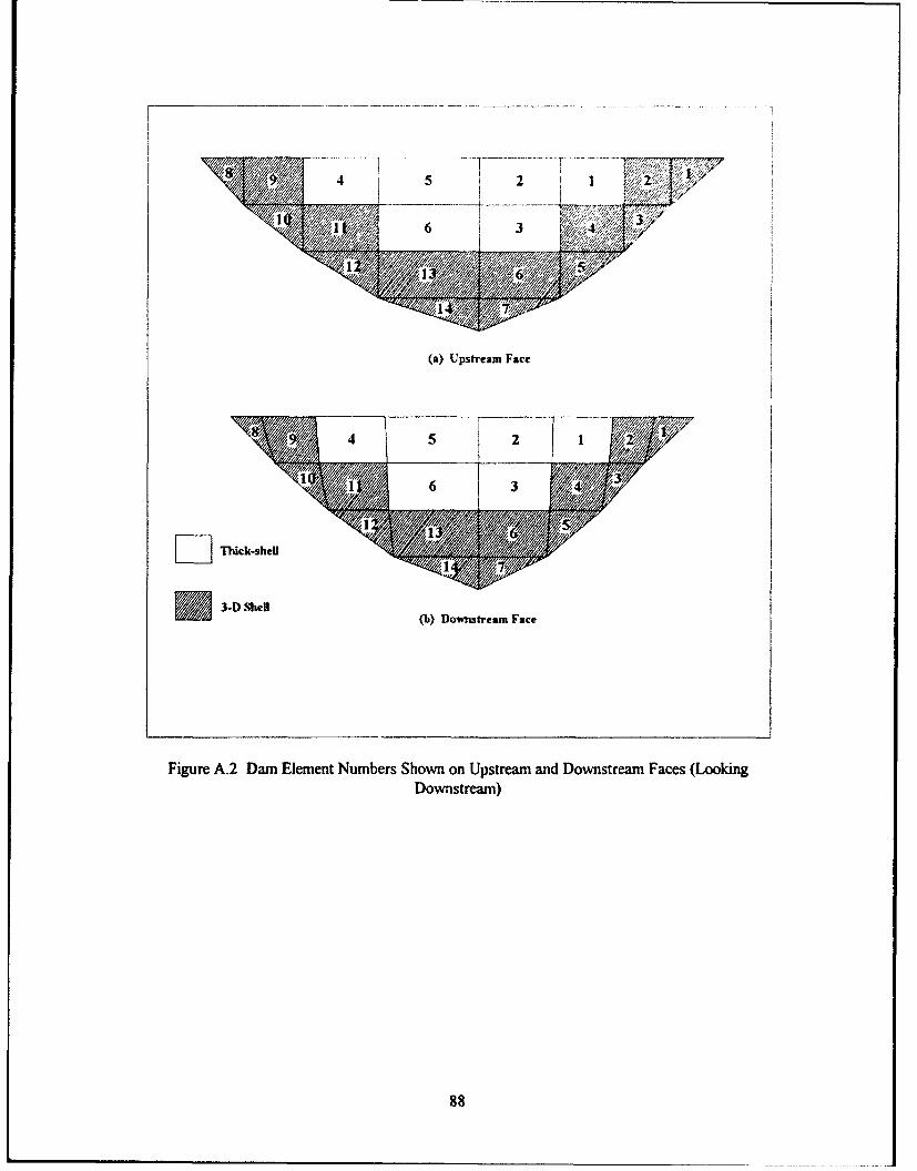
4 5 2 1 2
/ / ~6 3
(a) Upstream Face
W- Thick-shell
•]3-D Shell(b) Downstream Face
Figure A.2 Dam Element Numbers Shown on Upstream and Downstream Faces (LookingDownstream)
88
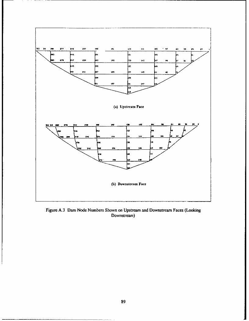
2 3 3 01 7 e 42 237 I" 11 141 439 97 43 V2 7
I M 51 95
27 4 210 3,5 Ii• 04347 994
My Z9 ?353 07,6
1 23 7 39537 345 U E
.5 247 ?67 347
147
(a) Upstream Face
314 2tt t22 4 22 R4 t"2 M5 141 304 9B 6 4 44 0 M6
44 5
M0 an9 49 £40 4:1 5 4 4 06 3 4R
24? 1%4 1 46 O210
0 44 14
(b) Downstrem Face
Figure A.3 Dam Node Numbers Shown on Upstream and Downstream Faces (LookingDownstream)
89
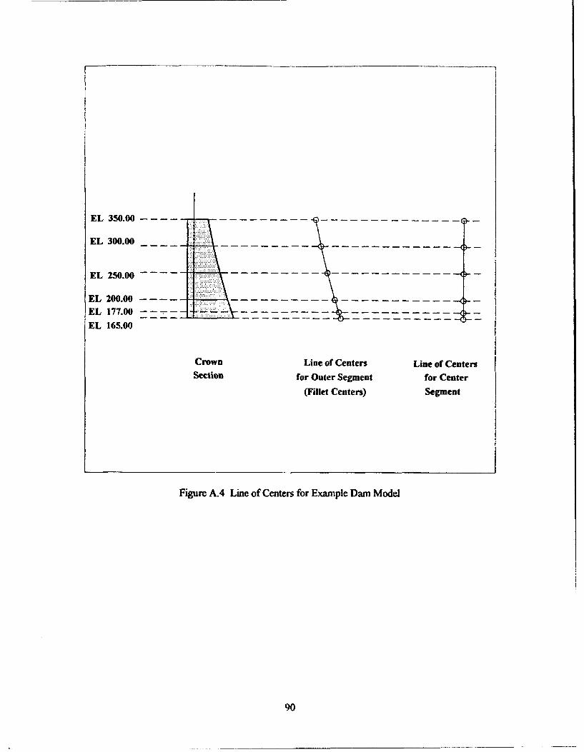
EL 350.00 --- - - -
EL 300.00 - - - - - -- -- ----- --- --- --
EL 250.00------- -- ----- - ----------- - ---- ------- ------ -----
EL 200.00 --
EL 177.00 ---
EL 165.00
Crown Line of Centers Line of Centers
Section for Outer Segment for Center
(Fillet Centers) Segment
Figure A.4 Line of Centers for Example Darn Model
90
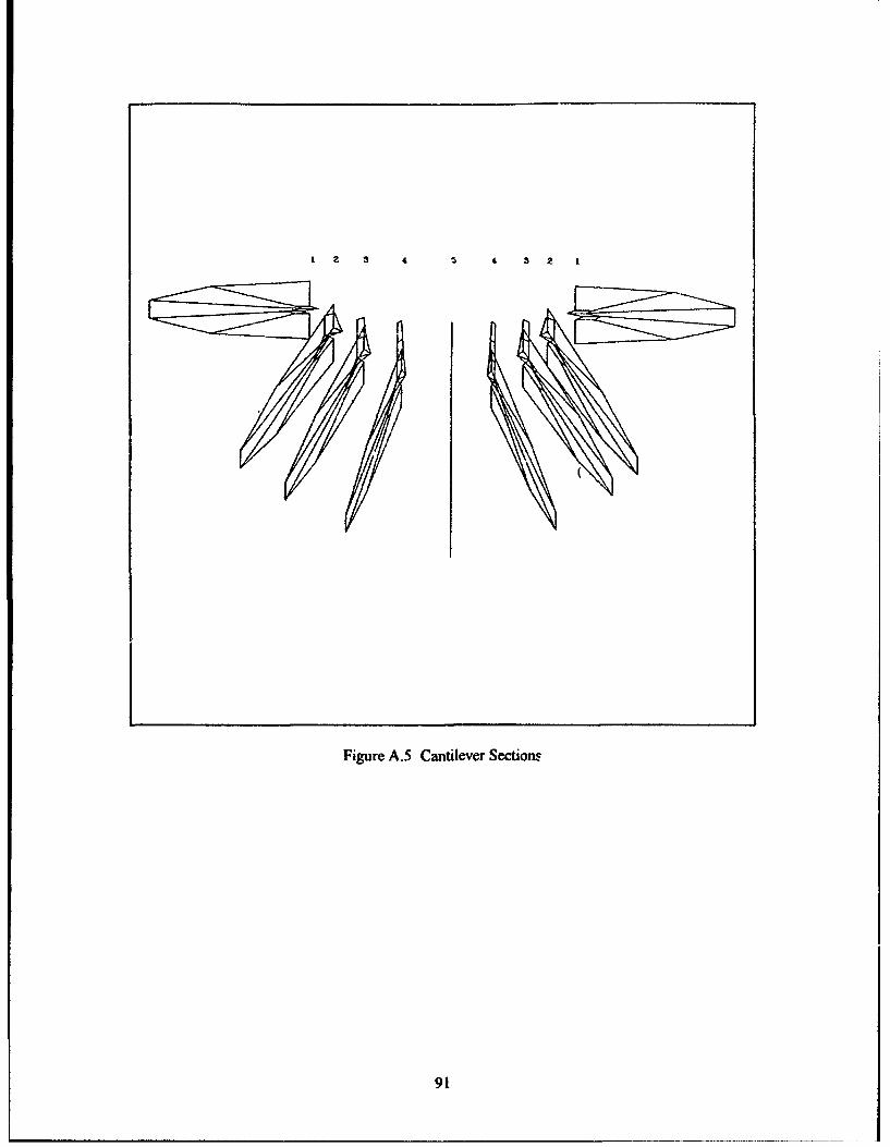
1 2 3 4 .3 4 3 2
Figure A.5 Cantilever Sections
91
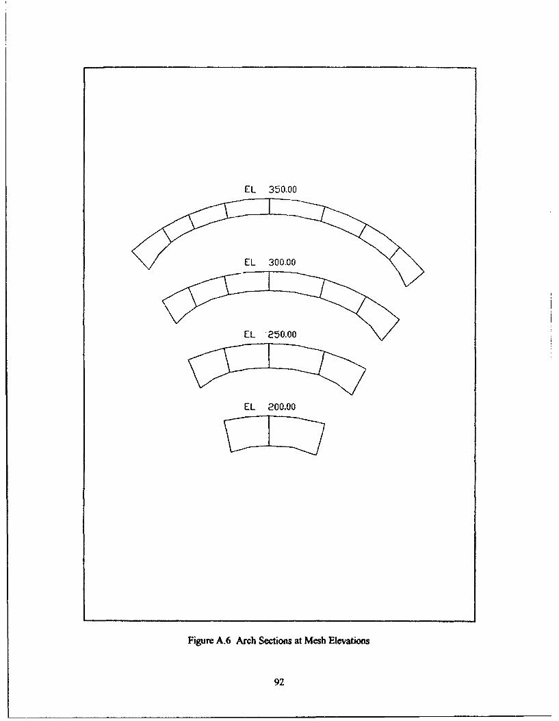
EL 350.00
EL 300.00
EL '250,00
EL 200.00
Figure A.6 Arch Sections at Mesh Elevations
92

~~~DAM .__
FOUNDATION
Figure A.7 Example Dam-Foundation Model (Hidden Lines Removed)
93

FOOTPRINT
FOUNDATIONROCK
Figure A.8 Example Foundation Model (Type 1)
94
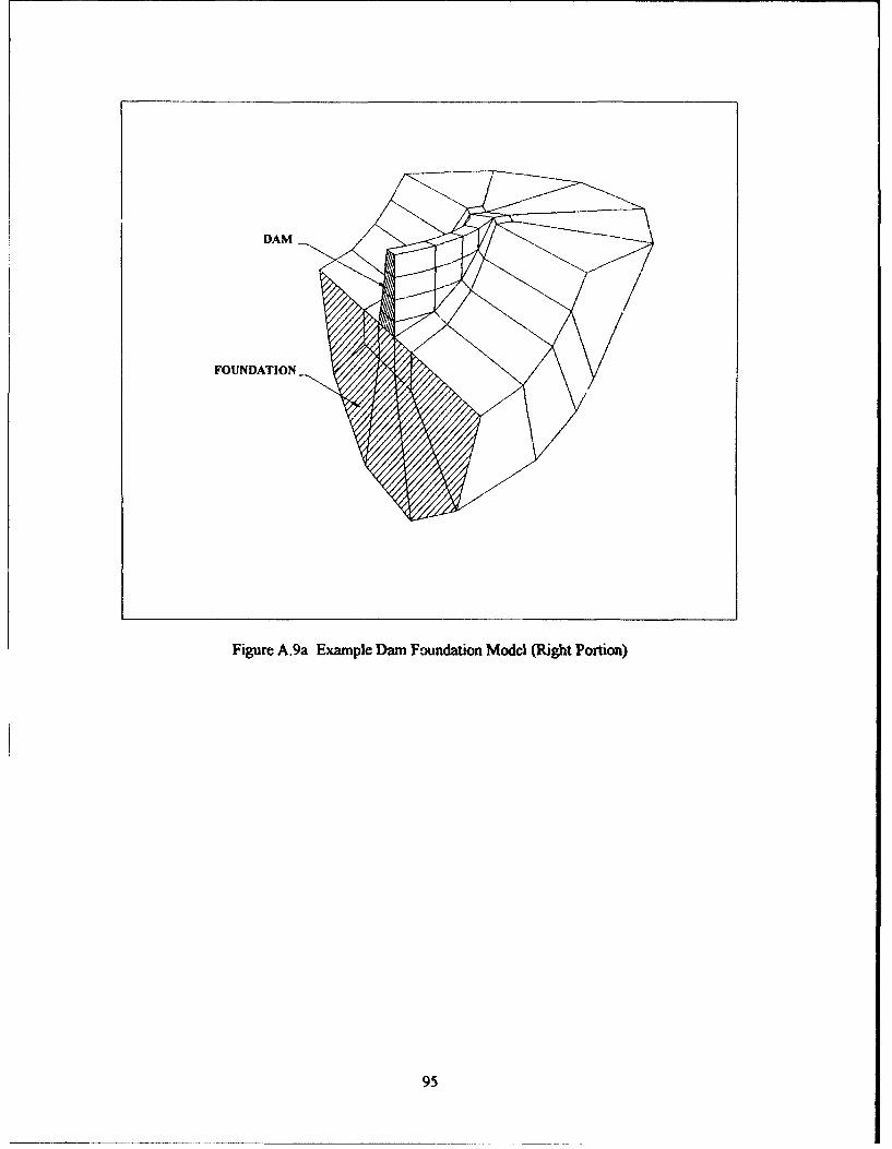
DAM
FOUNDATION
Figure A.9a Example Dam Foundation Model (Right Portion)
95

Figure A.9b Shrink Plot of Dan and Foundation Models
96
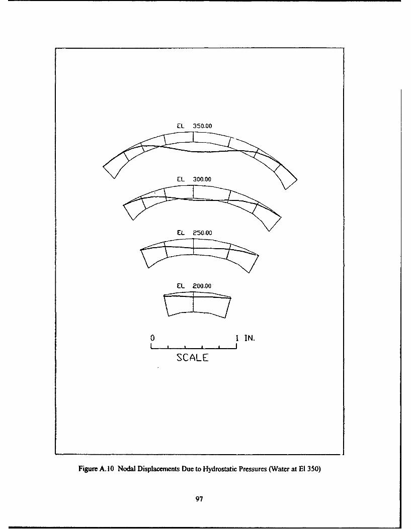
EL 350.00
EL 200.00
01 IN.
SCALE
Figure A. 10 Nodal Displacements Due to Hydrostatic Pressures (Water at El 350)
97

uw12. str
U/S Armh SUCnuc
dol2. atr
IDS Arch Svuem
Figure A. II Static Arch Stresses Due to Gravity + Hydrostatic Loads
98
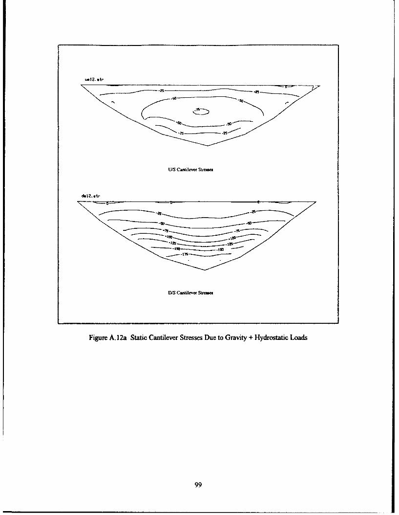
um12. atr
U/s Cantilever Stuam
do12. Mi-
-- IS
D/S Cantilever Sutss=
Figure A. 12a Static Cantilever Stresses Due to Gravity + Hydrostatic Loads
99
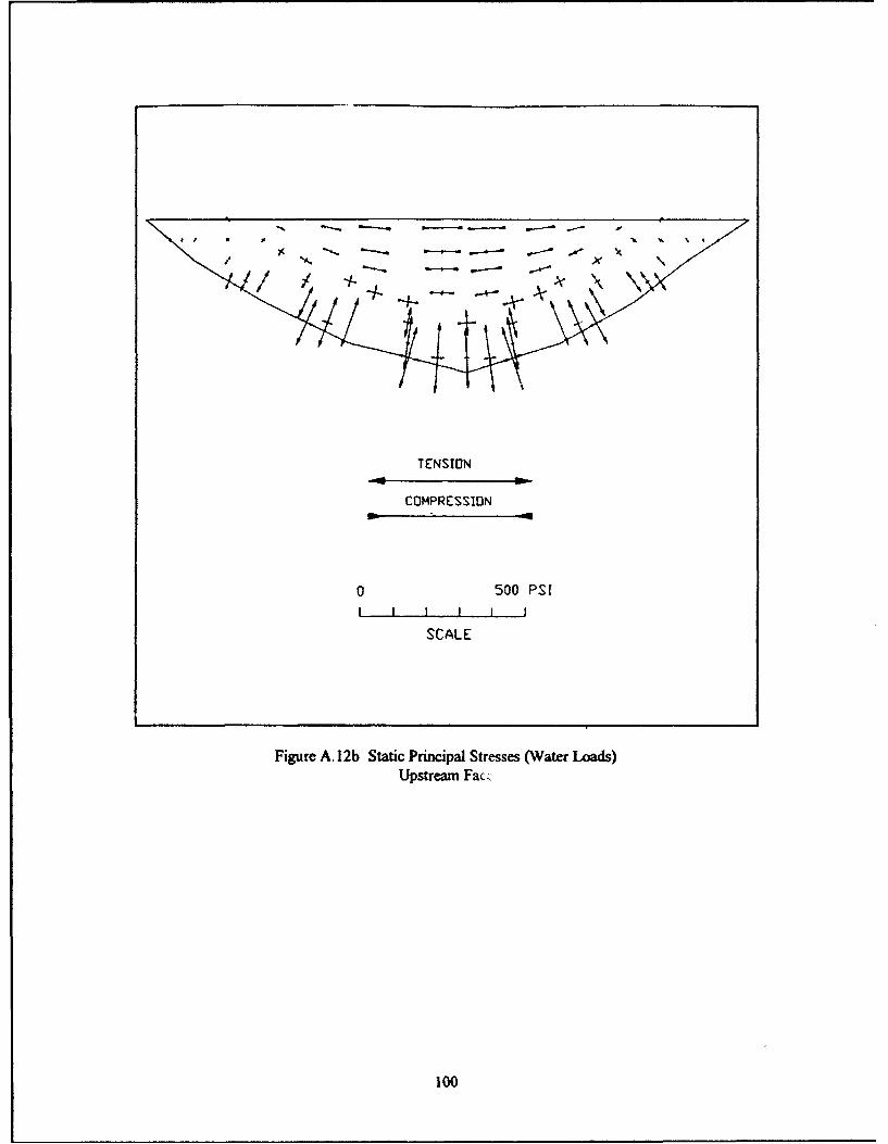
"" * x' \
TENSION
COMPRESSION
0 500 PSI
SCALE
Figure A. 12b Static Principal Stresses (Water Loads)Upstream Fac-
100
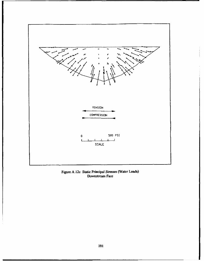
TENSION
COMPRESSION
0 500 PSII I I 1 ,I
SCALE
Figure A. 12c Static Principal Stresses (Water Loads)Downstream Face
10l

++ +1I4 ++I
SCALE
Figure A. 12d Static Principal Stresses (Gravity + Water)Upstream Face
102
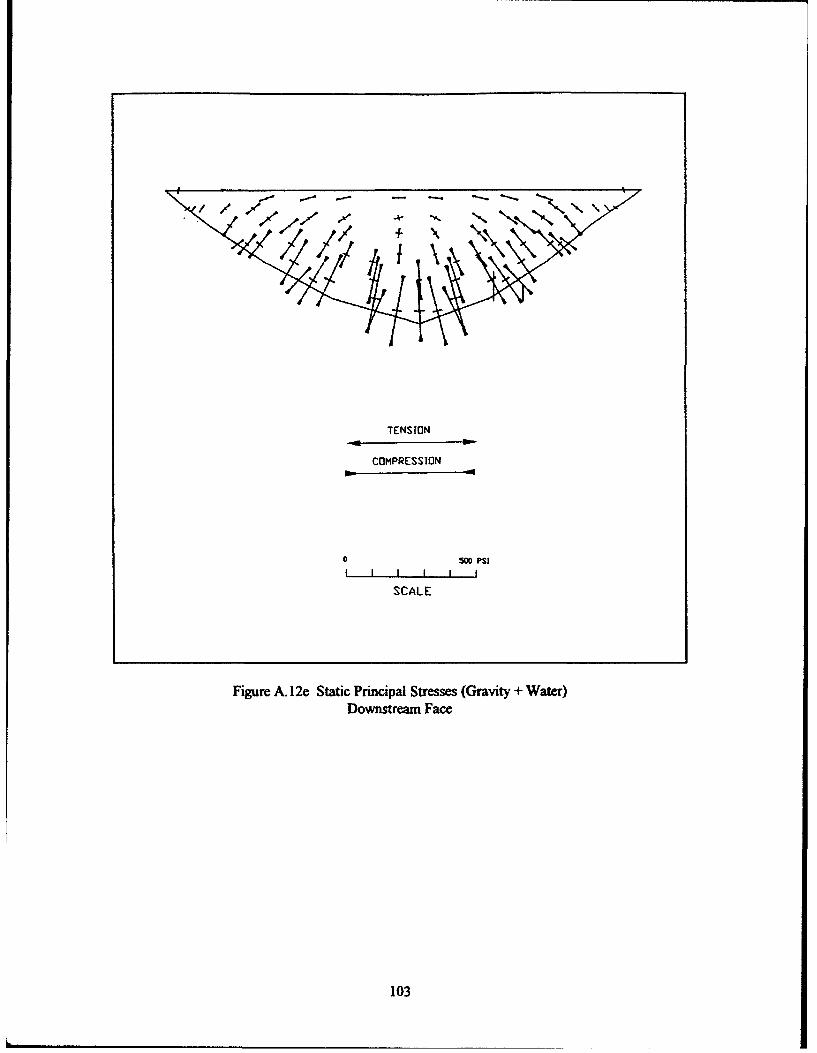
+7 \
TENSION
COMPRESSION
0 500Psi
I I I I I I
SCALE
Figure A. 12e Static Principal Stresses (Gravity + Water)Downstream Face
103

z
EL 350.00 ------------___------
EL 300.00 7~Z.-
EL 250.00 -- - - - -
EL 200.00 ---- --- --- ---
EL 16S.00---------------_ _ _
110
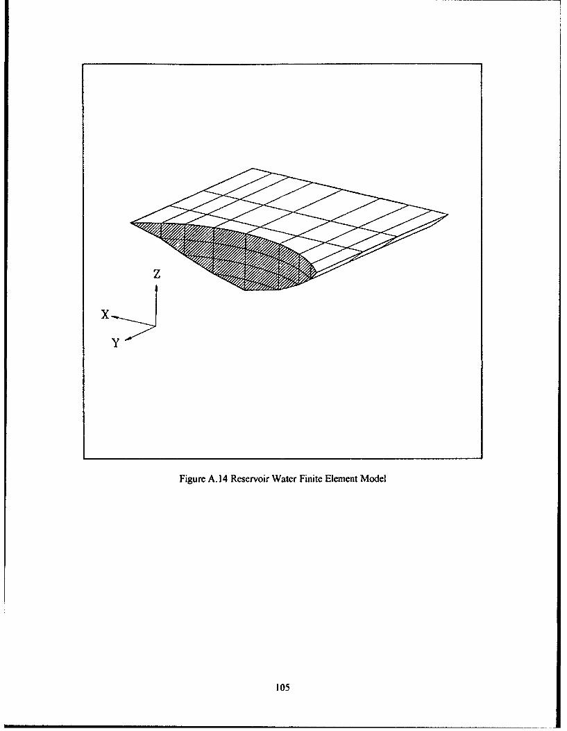
Figure A. 14 Reservoir Water Finite Element Model
105
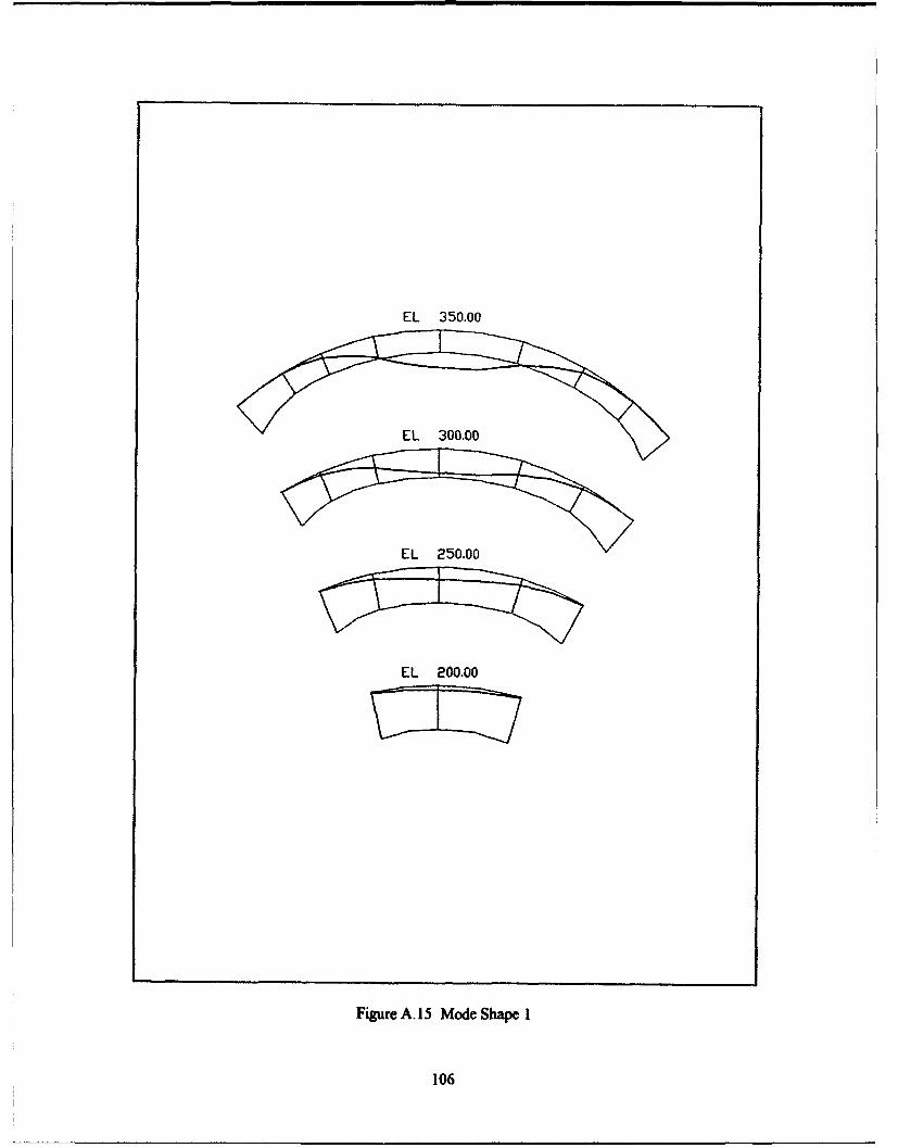
EL 350.00
EL 200.00
Figure A.15 Mode Shape I
106

EL 250.00
EL 200.00
Figure A. 16 Mode Shape 2
107
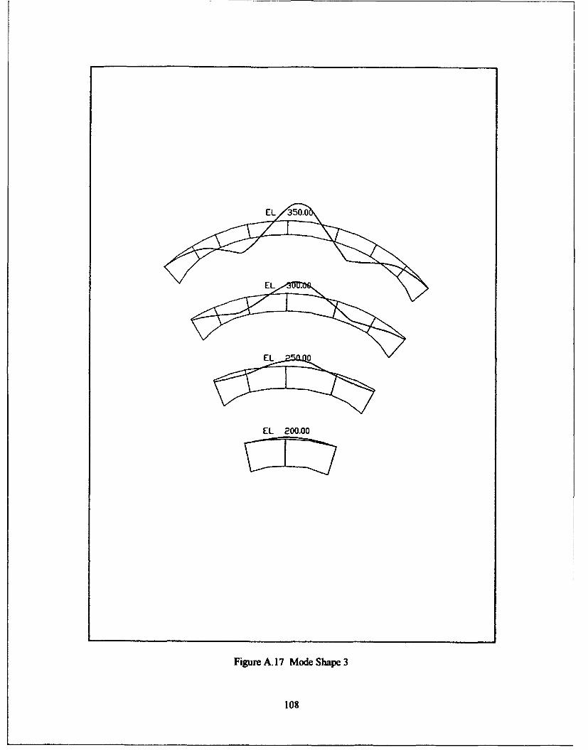
EL 200.00
Figure A.17 Mode Shape 3
108

EL 3~~o
EL 200.00
Figure A.18 Mode Shape 4
109
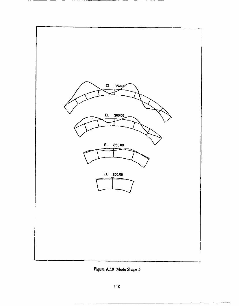
EL 300.00
EL 200.00
Figure A.19 Mode Shape 5
110
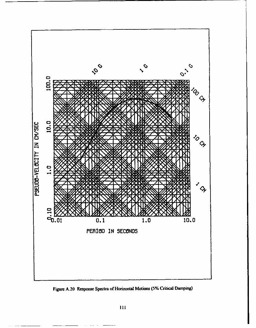
C)0
V) 0
CnC
SI
LiiZ-4
1o
toLIi
01 0.1 1.0 10.0
PERIOD IN SECONDS
Figure A.20 Response Spectra of Horizontal Motions (5% Critical Damping)
I11

0
1-4L)
Uid
(n D
':•0.I, 1l 41I1. 00
cn
0.10.1 1.0 10.0
PERIOD IN SECONDS
Figure A.21 Response Spectra of Vertical Motion (5% Critical Damping)
112
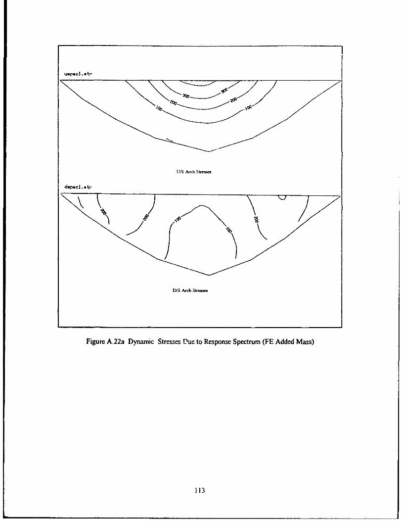
1?01
UIS Arch Str",scs
D/S Arch Strem=
Figure A.22a Dynamic Stresses Due to Response Spectrum (FE Added Mass)
113

U/S Aidi Sztucs
fl/S Arcb Stresu
Figure A,22b Dynamic Stresses Due to Response Spectrum(Westergaard Added Mass)
114
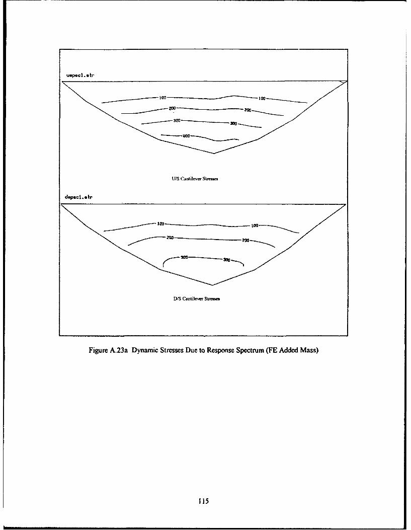
uepecl.etr
10010
3 00
U/S Cantilcvcr Stresses
dlpec • tr
100 a
200
DIS Cantilever Stro=
Figure A.23a Dynamic Stresses Due to Response Spectrum (FE Added Mass)
115
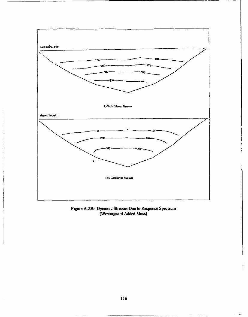
U/S C.uIca ?strcma
dopeciw. tr"
D/S Cantilcva Suezem
Figure A.23b Dynamic Stresses Due to Response Spectrum(Westergaard Added Mass)
116
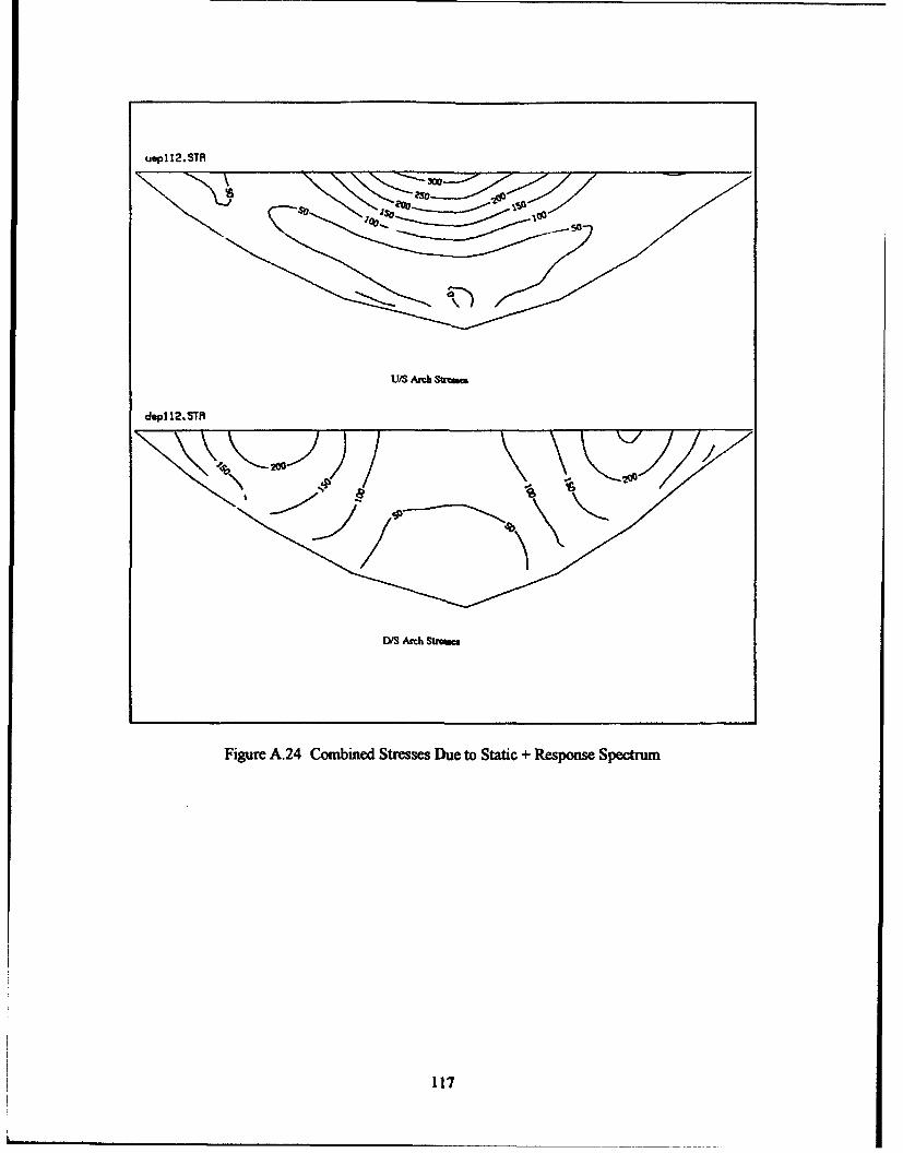
uq•ll2,STFI
uap112. SITR
U/S Armb Strbaua
dep 112. ST
12/S Afth Strcace
Figure A.24 Combined Stresses Due to Static + Response Spectrum
117

uspll2.ur
U/S Cantilcver st"M
dpl2. tr
100 00
D/S Cantilver Shreac
Figure A.25 Combined Stresses Due to Static + Response Spectrum
118

C3 STIW catEoNT
C3,
g0-
0.00 2.00 .00 6.00 8.00 10.00SECOND
w
C3.
*% 0
cuC6
0.00 2.00 I.00 6.00 8.00 10.00SECONDS
C!0m
0.00 2.00 tL.00 6.00 8.00 10.00SECONDS
Figure A.26 Time-fistories of Longitudinal Component of Earthquake Motion
119

o aiS-CAMa COMPOMeITC3
C3.I'" ' A' y'" '' l'.I, .
0
0.00 2.00 4.O0 6.00 8.00 10.00
SECONDS
9 "AJ 4 A "'i MA" I
1 Ap-4 A J & I V
0.00 2.00 1.00 6.00 8.00 10.00SECONDS
ru
V V [,I
0.00 2.00 4.00 6.00 8.00 10.00SECONDS
Figure A.27 Time-Histories of Transverse Component of Earthquake Motion
120
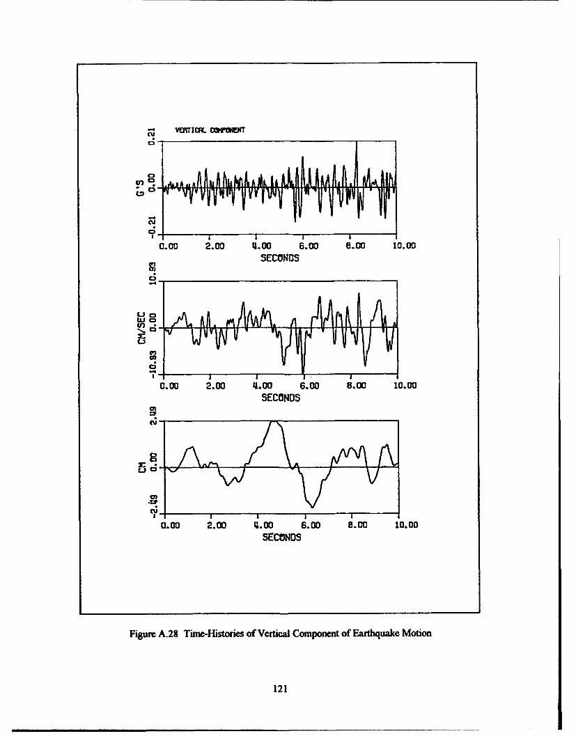
('- VERTICAL Car@EIIT
C4
-4
0.00 2.00 4.00 6.00 8.00 10.00SECONDS
;v V
0.00 2.00 41.00 6.00 8.00 10.00SECONDS
FiueA2 ieHsoie fVria)opnnto atqaeMto
:12
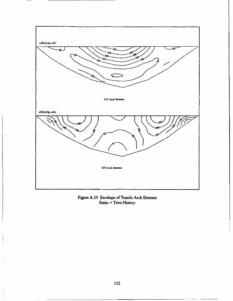
uthlstp.str
U/S Arch Strl=m=
dthi .tp. etr
( ISO
D/S Arch St•'sc
Figure A.29 Envelope of Tensile Arch StressesStatic + Time-History
122
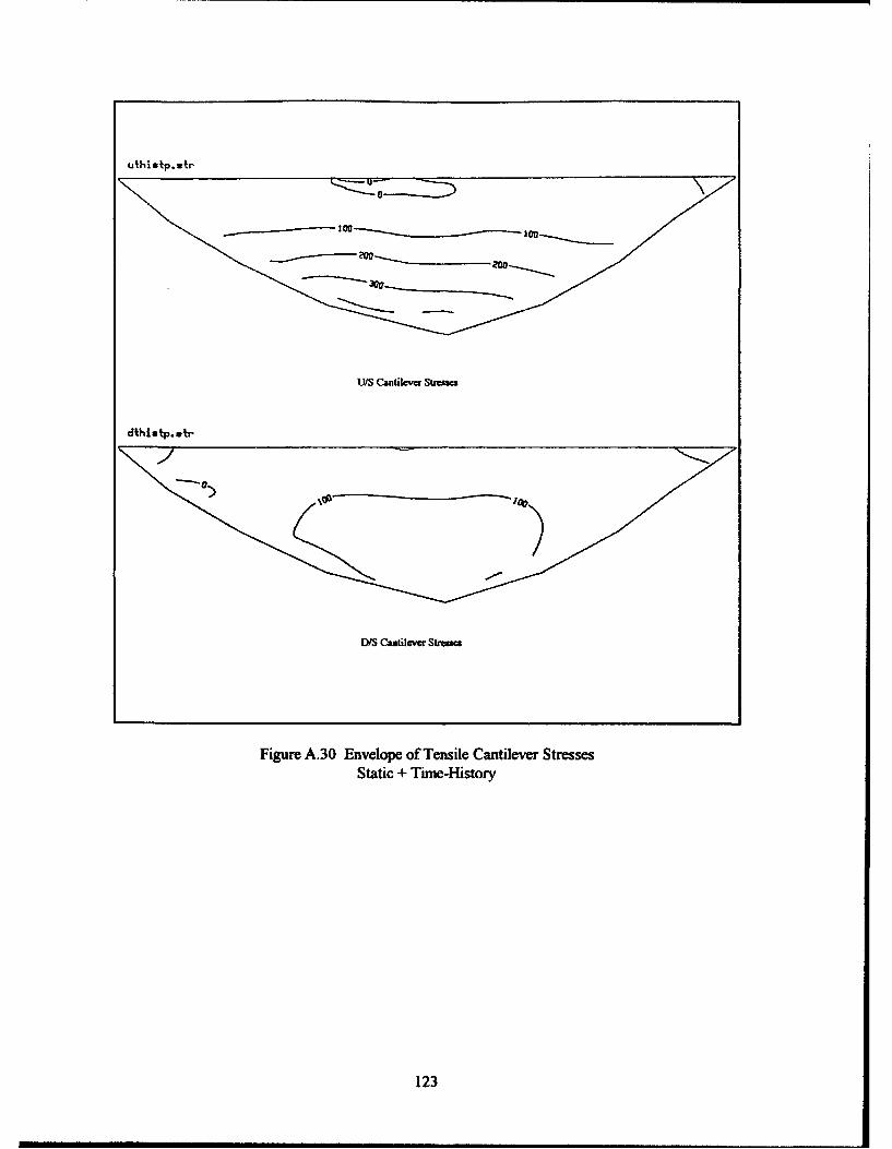
uthI atp.otr
U/S Cantilevr Strms•s
dthisatp.st
D/S Cantilcver Strme
Figure A.30 Envelope of Tensile Cantilever StressesStatic + Time-History
123

uconcur2.oatr
0 00
100
U/S Cantilcc Stinues
doancu2.otr
-200
D/S Cantileve Sueuca
Figure A.31 Concurrent Cantilever Stresses at Time 7.06 sec.Static + Time-Hfistory
124

uconcur3. tr
00
U/S Cantilcvr SUCa
dclcanes3. etr
-200 -- - - - -- 2--00
US lcatilce•rStmam
Figure A.32a Concurrent Cantilever Stresses at Time 8.70 sec.Static + Time-History
125
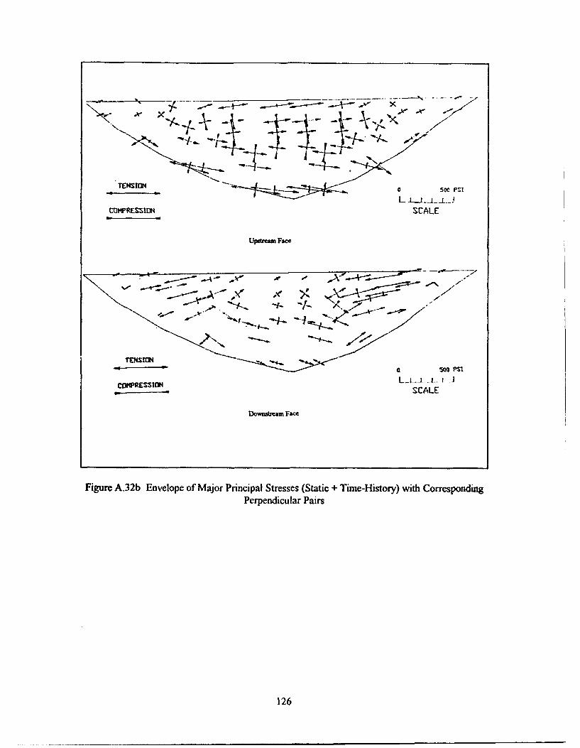
-ENI" 50 . PSI
I:OWIRESSlIO SC•ALE
Upsircam Face
""---------- -
-O-- ,. -- --.. JS•SCALE
Do'wwtcam FaceSC
L
Figure A.32b Envelope of Major Principal Stresses (Static + Time-History) with CorrespondingPerpendicular Pairs
126
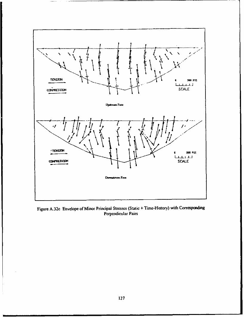
cO",ES"UI SCALE
Updm F,."
TENSt'I0 5w0 PSI
COPRESS" SCALE
UIream F&a=
Figure A.32c Envelope of Minor Principal Stresses (Static + Time-History) with CorrespondingPerpendicular Pairs
12"7

o N0E !U T-c•PtWO(N
z -
C:3
•0
0
0.00 1.25 2.50 3.75 5.00 6.25 7.50 8.75 10.00SECONDS
Wo #O-157 "T-CUiOtlNt
a0 0c
£0
0.00 1.25 2.SO 3.75 5.00 6.25 7.S0 8.75 10.00SECONDS
Figure A.33 Stream-Direction Displacement Time-Histories of Nodes 149 and 157, Located atCrest and Midheight Elevations, Respectively (Figure A.3)
128

w 3-SM*L 5W1 LE~tf ELM-? 5e-j
Allowa.ble Sress - 350 psi
I.- CO
0.00 1.25 2.50 3.7S S.00 6.25 7.5 6.75 10.00SECONDS
toM! 3D-SHEU. CWTILEVE1R ELK-'? S?-2
9 0
t4
0.00 1.2S 2.50 3.7S 5.00 6.25 7.So 8,7S 10.00SECONDS
Figure A.34 Time-Hfistory of Cantilever Stresses for Stress Points 1 and 2 (Located on UpstreamSide and Downstream Side) of 3-D Shell Element No. 7 (Figures 6.9 and A.2)
129

30-SHELL CMNILEVER ELM-1 SP-9
E Alovable Stress - 350 psi
-- - - - - - - --0
tu
0.00 1.25. 2.SO 3.75 5.00 6.25 7.50 8.75 10.00SECONDS
C13
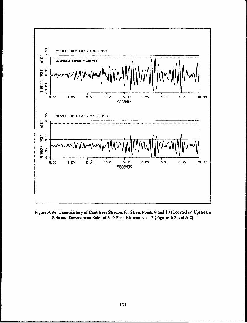
cu 30-SHiEL.L CANTILEVE71 E LK-12 :,''5-9inU Allowable Streass 350 psi
0.00 1.23 2.50 3.75 5.00 6.25 7.50 8.7p5 10.00
SECONDS
uLC 30-SIELL CMWI'LEVE1l t ELI-12 SP-i1
1-0
(n 9 a A_ . .AA
0.00 1.25 2.0 3.75 S.00 6.25 7.50 8.7S 10.00SECONDS
Figure A.36 Time-History of Cantilever Stresses for Stress Points 9 and 10 (Located on UpstreamSide and Downstream Side) of 3-D Shell Element No. 12 (Figures 6.2 and A.2)
131

Uin 30-IELL MRI:LEVE1I t ELI-IJ 3P-3
0All•1owable Stress - 350 pat
to0CC(n
ot o
0.00 1.25 2.50 3.75 5.00 6.25 7.50 8.75 10.00SECONDS
S30.-SELL MR1ILtEVER 0I-Il- SP-A
0)0
In*
0.00 1.25 2.50 3.75 5.00 6.25 7.50 8.75 10.00
SECONDS
Figure A.37 Time-History of Cantilever Stresses for Stress Points 3 and 4 (Located on UpstreamSide and Downstream Side) of 3-D Shell Element No. 14 (Figures 6.2 and A.2)
132
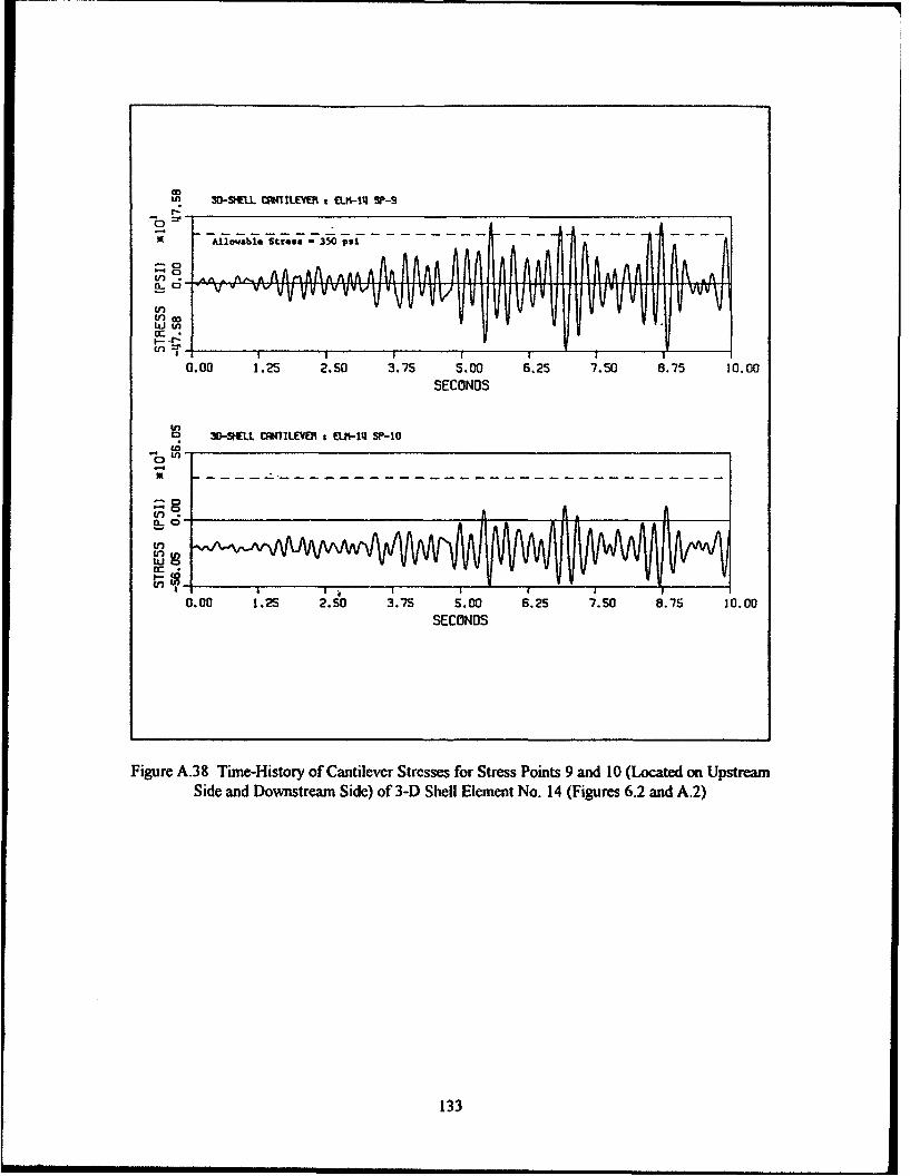
W SJ-S'ELL 1ILEVM E LU.-I-l SP-9
Aliovable Stress " Z35- ps-
VWVVVVVVVV4 " iV(n00
U,• :•,IUd tn
0.00 1.25 2.S0 3.7S 5.00 6.25 7.50 8.75 10.00
SECONDS
30SidEL and 4 zowstELM-1 Sid)oP-10 hl lmn o 4 Fgrs62adA2
1n-- -0StL -FI1LV? -EU-I s- - - - - - - - - - - --a
0.00 1.2S 2.50 3.75 5.00 6.25 7.50 8.75 10.00SECONDS
Figure A.38 Tune-History of Cantilever Stresses for Stress Points 9 and 10 (Located on UpstreamnSide and Downstream Side) of 3-D Shell Element No. 14 (Figures 6.2 and A.2)
133

REPORT DOCUMENTATION PAGE F
Puftw qalil mo " idget, t tw TIt cooteitOn of .ntom"6i tM il~f ha flI et to o£fetq I nlow Daf moIrAw. .fl(i4J0*q twie tamW fc r9ww 40 oIU(ftin ." looifugo aftlq Gtswt~ wurel.ý~~~~~ ~ ~ ~ ~ 4o up""f for r"av msor"aimo
"vMqhwý,&V.St) 1J04, ArI•qlon, VA 122024302, .nO to IF OtfiCe of Mn0qq0*01 si6 M &~ .Et Redi0tfl mFtb QA p r 07"4-010 11. *wevurqW . OC 20$01.
1. AGENCY USE ONLY (Leave Wlank) 2. REPORT DATE 3. REPORT TYPE AND DATES COVERED
August 1993 Final report4. TITLE AND SUBTITLE S. FUNDING NUMBERS
User's Manual - GDAP, Graphics-Based Dam Analysis ProgramVersion 3.25
G. AUTHOR(SI
Yusof Ghanaat
7. PERFORMING ORGANIZATION NAME(S) AND AOORESS(ES) 8. PERFORMING ORGANIZATIONREPORT NUMBER
Quest Structures1900 Powell St., Suite 210Emeryville, CA 94608
9. SPONSORING I MONITORING AGENCY NAME(S) AND ADDIOSS(ES) 10. SPONSORING / MONITORING
U.S. Army Corps of Engineers, Washington, DC 20314-1000; AGENCY REPORT NUMBER
U.S. Army Engineer Waterways Experiment Station, Information Technology Instruction Report ITL-93-3
Laboratory, 3909 Halls Ferry Road, Vicksburg, MS 39180-6199
11. SUPPMEMENTARY NOTES
See reverse.
124. OISTRIBUTION / AVAILABIUTY STATEMENT 12b. DISTIBUTION CODE
Approved for public release; distribution is unlimited.
13. ABSTRACT (M•a•um 200 wom)
This manual describes the graphics-based dam analysis program (GDAP) which performs three-dimen-sional (3-D), finite element (FE) static and dynamic analyses of concrete arch and gravity dams on a desktopcomputer and provides graphic pre- and post-processing capabilities. The FE meshes of the concrete dam,foundation rock, and the impounded water are generated automatically from a limited amount of input data.Various two- (2-) and 3-D graphics are produced to examine the accuracy of the analytical models. The re-sults of static and dynamic analyses are displayed in graphical forms for easy interpretation and evaluation.In particular, the GDAP post-processor automatically evaluates the response-history results and extracts thecritical information for presentation and further evaluation.
114. SUBJECT TERMS 15. NUMBER OF PAGES
Arch dam 141
Dynamic analysis 11. PRICE COwE
1U. SECURITY IED1 CL ATSS ION 1111. SECUJRT CLASSIFICATIO . SECURTY CLASSIFICATION 20. UMITATION Of ABSTRACTOF REPORT OF THIS PAGEPATO 19 Of ABSTRACT
UNCLASSFD UNCLASSIFIED s ______________
NSN ?Sd0O-G.-JB@-SSO0-StanMrd Form 2" IRtw. 2-9)
-Jwh f US f

11. (Concluded).
The User's Manual is available from National Technical Information Service, 5285 Port Royal Road,Springfield, VA 22161. The computer program is available to U.S. government employees only and canbe obtained through the Engineering Computer Program Library at the U.S. Army Engineer WaterwaysExperiment Station, 3909 Halls Ferry Road, Vicksburg, MS 39180-6199.