© copyright 2016 chi ho eric cheung
TRANSCRIPT

© Copyright 2016
Chi Ho Eric Cheung

Delamination Arrestment in Bonded-Bolted Composite Structures by Fasteners
Chi Ho Eric Cheung
A dissertation
submitted in partial fulfillment of the
requirements for the degree of
Doctor of Philosophy
University of Washington
2016
Reading Committee:
Kuen-Yuan Lin, Chair
Eli Livne
Mark E. Tuttle
Program Authorized to Offer Degree:
Aeronautics and Astronautics

ii
University of Washington
Abstract
Delamination Arrestment in Bonded-Bolted Composite Structures by Fasteners
Chi Ho Eric Cheung
Chair of the Supervisory Committee:
Professor Kuen-Yuan Lin
William E. Boeing Department of Aeronautics and Astronautics
Laminated composites have exceptional in-plane strengths and fatigue properties. However, they
are susceptible to the interlaminar mode of failure, namely disbond and delamination. This
failure mode challenges the edges of structural interface, such as the skin-stringer flange and run-
out, where interlaminar tension, shear, and opening moment are concentrated. The fasteners
provide a substantiation path for the FAA damage tolerance requirement for composite bonded
joints (FAR 23.573).
A comprehensive understanding of delamination arrestment by fasteners was developed. The
fastener provides crack arrest capability by three main mechanisms: 1) mode I suppression, 2)
crack-face friction, and 3) fastener joint shear stiffness. The fastener mechanically closes the
crack tip, suppressing mode I fracture and forcing the crack to propagate in pure mode II with
higher fracture toughness. Fastener preload generates significant friction force on the cracked

iii
surfaces which reduces crack-tip forces and moments. The fastener shear joint provides an
alternate load path around the crack tip that becomes more effective as crack length increases.
The three mechanisms work in concert to provide various degrees of crack arrestment and
retardation capability.
A novel test technique was developed to quantify the delamination arrestment capability by
fasteners under in-plane dominated loading, i.e. mode II propagation. The test results show that
the fastener is highly capable of delamination arrestment and retardation. The test also
demonstrates that fastener installation preload, which is directly related to crack-face friction, is
an important factor in delamination arrestment.
A computationally efficient analytical method was developed to capture the behavior and
efficacy of delamination arrestment by fasteners. The solution method is based on the principle
of minimum potential energy and beam-column modeling of the delaminating structure. The
fastener flexibility approach is used to provide implicit modeling of the fastener, while a closed-
form crack-tip element is used to calculate the mixed-mode strain energy release rates at the
crack tip. The analytical method correlates well to the test results. The analytical method is used
in parametric studies to expand the understanding of the delamination arrest fastener, such as
sensitivities to fastener diameter and fastener hole clearance.

iv
TABLE OF CONTENTS
List of Figures ................................................................................................................................ vi
List of Tables .................................................................................................................................. x
Acknowledgement ........................................................................................................................ xii
Chapter 1. Introduction ............................................................................................................... 1
Chapter 2. Literature Review...................................................................................................... 5
2.1 On Interlaminar Fracture Methods ................................................................................... 5
2.2 On Implicit Fastener Modeling ........................................................................................ 6
2.3 On Hybrid Bolted-Bonded (HBB) Joining Technology .................................................. 6
2.4 On Experimental Methods ............................................................................................... 7
Chapter 3. Finite Element Modeling ........................................................................................ 11
3.1 Split-Beam Model Description ....................................................................................... 12
3.2 Material Properties ......................................................................................................... 16
3.3 The Finite Element Model .............................................................................................. 19
3.4 Results and Discussions ................................................................................................. 21
3.4.1 Effect of Fastener under Mode I Loading ............................................................... 22
3.4.2 Effect of Fastener under Mixed-Mode Loading ..................................................... 24
3.4.3 Effect of Contact Friction and Fastener Preload under Mixed-Mode Loading ...... 28
3.4.4 Discussion of the Main Crack Arrest Mechanisms ................................................. 32
3.4.5 Alternate Failure Modes not Considered in the Current Analysis .......................... 34
Chapter 4. Development of the Analytical Method .................................................................. 36
4.1 Analytical Model and Modeling Assumptions ............................................................... 36
4.2 Solution Method: Rayleigh-Ritz Method (PMPE) ......................................................... 43
4.3 Numerical Implementation ............................................................................................. 52
4.4 Validate Analytical Beam-Column Solution with FEA ................................................. 57
4.4.1 Deflection of a Single Composite Beam-Column .................................................. 58

v
4.4.2 Deflection of a Composite Split-Beam ................................................................... 63
4.4.3 Fastener Joint Shear Load and Mode II Strain Energy Release Rate (GII) ............. 69
Chapter 5. Single-Fastener Two-Plate Delamination Arrest Test ............................................ 81
5.1 The Need for a Novel Test Design ................................................................................. 81
5.2 Configuration, Fabrication, and Testing of the Delamination Arrest Specimen ............ 82
5.3 Test Results .................................................................................................................... 91
5.4 Crack Propagation Behavior Discussion ...................................................................... 105
5.5 Correlation of Analytical Method to Test Data ............................................................ 112
Chapter 6. Sensitivity/Parametric Study Using the Analytical Method ................................. 125
6.1 Crack Propagation Parametric Study ........................................................................... 126
6.2 Sensitivity Analysis – Design Space Study.................................................................. 133
6.3 Probabilistic Analysis ................................................................................................... 141
Chapter 7. Discussions on Practical Application of Delamination Arrest Fasteners ............. 150
7.1 The Need for Delamination Arrest Fasteners ............................................................... 150
7.2 Defining the “Arrest” in Arrest Capability .................................................................. 151
7.3 Expectation of Benefit from Crack Arrest Fasteners in the Arrested Phase ................ 152
7.4 Critical Parameters for Design and Analysis ............................................................... 153
Chapter 8. Conclusions ........................................................................................................... 155
References ................................................................................................................................... 159
Appendix A – Raw Propagation Load Data ............................................................................... 162
Appendix B – Obtaining the MATLAB Source Code ................................................................ 168

vi
LIST OF FIGURES
Figure 1. Schematic of the ENF Test .............................................................................................. 8
Figure 2. Schematics of Symmetric Mode II Delamination Arrest Specimen Designs ................ 10
Figure 3. Diagram of the Crack Arrest Finite Element Model ..................................................... 13
Figure 4. Contact Forces in the Fastener and Plates in Single Shear ............................................ 15
Figure 5. Net Forces and Moments in the Fastener in Single Shear ............................................. 15
Figure 6. Spring Load-Displacement Curve for Fastener with Preload ........................................ 18
Figure 7. Finite Element Mesh of the Split-Beam Model (Deformed under Mode I Loading) .... 19
Figure 8. Finite Element Mesh of the Split-Beam Model (Enlarged Near the Crack Tip) ........... 20
Figure 9. Propagation Moment vs. Crack-Tip Location in Mode I .............................................. 23
Figure 10. Deformation of a DCB with Fastener with Applied Tension on the Lower Beam ..... 24
Figure 11. Propagation Load vs. Crack-Tip Location in Mixed-Mode ........................................ 26
Figure 12. SERR Components Required for Propagation vs. Crack-Tip Location in Mixed-Mode..................................................................................................................................... 27
Figure 13. Propagation Load vs. Crack-Tip Location in Mixed-Mode with Preload and Contact Friction ........................................................................................................................ 31
Figure 14. Schematic of Analytical Model ................................................................................... 37
Figure 15. Beam-Column Model – Bending Deflection and Interactions in the Z-Direction ...... 38
Figure 16. Beam-Column Model – Axial Extension and Interactions in the X-Direction ........... 38
Figure 17. Fastener Preload Modeling .......................................................................................... 40
Figure 18. Fastener Shear Joint with Friction and Hole Clearance Modeling .............................. 42
Figure 19. Flow Diagram of the Analytical Method Implementation .......................................... 56
Figure 20. Deflection Validation – Single Beam Model .............................................................. 58

vii
Figure 21. Deflection Validation – Deflection Plots for Single Beam – Layup A ....................... 61
Figure 22. Deflection Validation – Deflection Plots for Single Beam – Layup B ....................... 62
Figure 23. Deflection Validation – Deflections Plots for Single Beam – Layup C ...................... 62
Figure 24. Deflection Validation – Split-Beam Model ................................................................. 63
Figure 25. Deflection Validation – Deflection Plots for Split-Beam – Layup A ......................... 67
Figure 26. Deflection Validation – Deflection Plots for Split-Beam – Layup B .......................... 68
Figure 27. Flexible Crack Tip (FEM) versus Rigid Crack Tip (Analytical Model) ..................... 69
Figure 28. Joint Shear Load and GII Validation – Crack Arrest Fastener Model ......................... 70
Figure 29. Example of Deformed Shape of the Analytical Model ............................................... 72
Figure 30. Joint Shear Load versus Crack-Tip Location (Lc) Validation – Sensitivity to Fastener Diameter ...................................................................................................................... 74
Figure 31. Joint Shear Load versus Crack-Tip Location (Lc) Validation – Sensitivity to Applied Load ............................................................................................................................ 74
Figure 32. GII versus Crack-Tip Location (Lc) Validation – Sensitivity to Fastener Diameter .... 78
Figure 33. GII versus Crack-Tip Location (Lc) Validation – Sensitivity to Applied Load ........... 78
Figure 34. Drawing of the Tension Crack Arrest Test Specimen (not to scale) ........................... 82
Figure 35. Specimen with Drilled Hole and Painted Scale (inches) on the Edge ......................... 85
Figure 36. Specimen with Fastener Installed (Left: Fastener Head Side; Right: Fastener Collar Side) ............................................................................................................................ 86
Figure 37. Visual Tracking of Crack-Tip Location – Crack Arrested at the Fastener .................. 87
Figure 38. Visual Tracking of Crack-Tip Location – Propagated Past the Fastener .................... 88
Figure 39. Specimen being Loaded in the Instron 5585H Test Machine ..................................... 90
Figure 40. Specimen Ultimate Failure – Filled-Hole Tension Failure ......................................... 92
Figure 41. Specimen Ultimate Failure – Filled-Hole Tension Mixed with Laminate Delamination/Splitting ................................................................................................ 92

viii
Figure 42. Applied Load vs. Crack-Tip Location – Short Panel (quasi-isotropic layup) ............. 97
Figure 43. Applied Load vs. Crack-Tip Location – Short Panel (50% 0-deg layup) ................... 98
Figure 44. Applied Load vs. Crack-Tip Location – Long Panel (quasi-isotropic layup) ........... 101
Figure 45. Applied Load vs. Crack-Tip Location – Long Panel (50% 0-deg layup) ................. 102
Figure 46. Improvements in Load Capability vs. Fastener Torque ............................................ 104
Figure 47. Photo of Specimen Showing Crack Interface Migration during Propagation ........... 105
Figure 48. Crack Propagation Behavior – Crack Front Geometries ........................................... 108
Figure 49. Crack Propagation Behavior with Arrest Fastener .................................................... 109
Figure 50. C-Scan Example of Crack Front Geometries with and without a Crack Arrest Fastener................................................................................................................................... 110
Figure 51. Schematic of Analytical Model for Test Correlation ................................................ 113
Figure 52. Fastener Joint Shear Flexibility – Under Cyclic Loading [13] .................................. 116
Figure 53. Fastener Joint Shear Flexibility – Under Quasi-Static Loading [13] ........................ 117
Figure 54. Analytical Method vs. Test Results – Short Panel Quasi-isotropic Layup ............... 121
Figure 55. Analytical Method vs. Test Results – Short Panel 50% 0-deg Layup ....................... 122
Figure 56. Analytical Method vs. Test Results – Long Panel Quasi-isotropic Layup................ 123
Figure 57. Analytical Method vs. Test Results – Long Panel 50% 0-deg Layup ....................... 124
Figure 58. Schematic of Analytical Model Used in Parametric and Probabilistic Study ........... 127
Figure 59. Crack Propagation Curves for Varying Fastener Sizes – Constant Width ................ 131
Figure 60. Crack Propagation Curves for Varying Fastener Sizes – Constant Fastener Spacing................................................................................................................................... 131
Figure 61. Crack Propagation Curves for Varying Fastener Hole Clearance ............................. 133
Figure 62. Configuration Used in Design Space Study .............................................................. 134
Figure 63. Coefficients of Correlation – Design Space Study .................................................... 140

ix
Figure 64. Histogram of Failure Loads for Each Failure Mode ................................................. 146
Figure 65. Coefficients of Correlation – Probabilistic Analysis ................................................. 148

x
LIST OF TABLES
Table 1. Carbon Fiber Reinforced Plastic Laminar Material Properties (AS4/3501-6) ............... 17
Table 2. Analytical Model Validation – Single Beam – Effective Laminate Properties .............. 59
Table 3. Analytical Model Validation – Single Beam – Load Cases ........................................... 59
Table 4. Analytical Model Validation – Single Beam – Tip Deflections ..................................... 61
Table 5. Analytical Model Validation – Split-Beam – Effective Laminate Properties ................ 64
Table 6. Analytical Model Validation – Split-Beam – Load Cases .............................................. 64
Table 7. Analytical Model Validation – Split-Beam – Tip Deflections ....................................... 66
Table 8. Joint Shear Load and GII Validation – Effective Laminate Properties ........................... 70
Table 9. Joint Shear Load and GII Validation – Fastener Axial and Shear Springs Constants ..... 71
Table 10. Joint Shear Load versus Crack-Tip Location (Lc) at N2=89.0kN ................................ 75
Table 11. Joint Load versus Crack-Tip Location (Lc) with Fastener Diameter = 6.35mm .......... 76
Table 12. GII versus Crack-Tip Location (Lc) at N2=89.0kN ....................................................... 79
Table 13. GII versus Crack-Tip Location (Lc) with Fastener Diameter = 6.35mm ....................... 80
Table 14. Summary of Test Final Failure Loads .......................................................................... 93
Table 15. Properties Used in Test Correlation Analytical Model ............................................... 114
Table 16. Properties Used in Parametric Studies ........................................................................ 128
Table 17. Input Parameters for Design Space Study – Uniform Distribution ............................ 135
Table 18. Input Parameters for Design Space Study – Constants ............................................... 136
Table 19. Summary of Design Space Study – Failure Loads ..................................................... 137
Table 20. Input Parameters for Probabilistic Analysis – Normal Distribution ........................... 142
Table 21. Input Parameters for Probabilistic Analysis – Constants ............................................ 143

xi
Table 22. Deterministic Failure Loads ........................................................................................ 143
Table 23. Summary of Probabilistic Analysis ............................................................................ 145

xii
ACKNOWLEDGEMENTS
I would like to thank my colleagues Phillip Gray and Erik Bruun, who walked the challenging
path of graduate research with me. I would also like to thank Professor Mark Tuttle and Bill
Kuykendall at the Mechanical Engineering Department, and Professor Brian Flinn and Ashley
Tracy at the Material Science Department, for providing help in composites manufacturing and
testing. Special thanks go to Gerald Mabson, Marc Piehl, Matt Dilligan, and Eric Cregger for
providing technical support and industry experience. Finally, I want to express my utmost
appreciation to my advisor, Professor Kuen Y. Lin, who has never given up on me.
This research is jointly supported by the Boeing Company and the Federal Aviation
Administration.
1
Chapter 1. Introduction
The use of composites in aircraft has enabled the use of bonded (co-cured, co-bonded or
secondary bonding) structures, the main advantages of which are reduction of part counts and
weight. Such integrated structures, as opposed to assembled structures, eliminate the need for
fasteners/rivets, reducing the cost and complexity associated with the legacy design approach.
A critical damage mode in a composite structure is disbond and delamination. Interlaminar
tension and opening moment are higher at discontinuities such as stringer flanges and run-outs,
inducing delaminations at these locations. Damage can also occur due to discrete source damage
such as impact and collision. This type of damage has the potential to propagate along the entire
interface under static or fatigue loads. Complete disbond of components, such as stringers, can
cause failure at the structural level even though the individual components remain intact.
In metallic airplane structures, the primary mechanism for crack initiation is fatigue cracks
emanating from rivet holes or areas of stress concentrations. The damage tolerance design
methodology was developed to address the safety evaluation of structure under fatigue. Initial
flaws are assumed to exist in any structure, and such flaws are assumed to grow into cracks and
propagate with cyclic loading. An inspection and repair program is in place to detect and repair
these cracks before they reach a critical size, i.e. the size at which the residual strength of the
structure drops below regulatory load. This approach requires extensive knowledge of crack
growth behavior and residual strength by the designers and a coordinated inspection and repair
program carried out by the operators.

2
The FAR Part 23.573 [1] specifies an additional set of requirements for damage tolerance and
fatigue evaluation of composite structures. The bonded joint requirement, which covers co-cured,
co-bonded, and secondary bonded structures, states that:
For any bonded joint, the failure of which would result in catastrophic loss of the airplane,
the limit load capacity must be substantiated by one of the following methods –
i. The maximum disbonds of each bonded joint consistent with the capability to
withstand the critical limit flight loads (design limit load) must be determined by
analysis, tests, or both. Disbonds of each bonded joint greater than this must be
prevented by design features; or
ii. Proof testing must be conducted on each production article that will apply the critical
limit design load to each critical bonded joint; or
iii. Repeatable and reliable non-destructive inspection techniques must be established
that ensure the strength of each joint.
Of the three substantiation methods, method (ii) is generally impractical for the production of
large commercial jets, while the inspection technology for method (iii) is currently still in
research and development. Today, only method (i) presents a viable substantiation path,
requiring design features to be installed in the structure to arrest disbonds. One example of such
design feature is the fastener.
In aircraft structures, it is common to use fasteners for assembly (e.g. fuselage skin-stringer-
frame attachments, wing skin-rib attachments). These fasteners also perform as a delamination
arrest feature. The benefit of using assembly fasteners is that the arrest capability comes for free,

3
while alternatives such as z-pin and z-stitching add cost and complexity to manufacturing.
Alternatively, fasteners may be added along a bondline for the sole purpose of disbond
arrestment; these fasteners would carry no load unless there is disbond damage. Another
advantage of fasteners is that they can be installed any time after the structure is cured, during
manufacturing or revenue service, providing greater flexibility in usage. For example, fasteners
can be installed at a damaged location on an in-service structure to prevent further growth,
delaying or eliminating the need for expensive repairs.
The effective use of fasteners as disbond/delamination arrest features requires comprehensive
understanding of their arresting capability and limitations, as well as an analysis method that can
be used for design. Disbond arrest under mode I loading is well understood. The high axial
stiffness of a fastener is effective in completely arresting mode I propagation, preserving the
integrity of rest of the bonded joint. However, disbond arrest under mode II/III loadings is not as
well understood, and it is difficult to predict the efficacy of arrest features such as fasteners.
Therefore, it is important to understand the underlying physics of fasteners in arresting disbonds
to fully realize their benefits while ensuring safety of the structure. This research focuses on the
investigation of the effectiveness of fastener as a disbond/delamination arrest mechanism and the
development of an analytical solution method for the problem.
A literature review of interlaminar fracture methods, fastener modeling, bonded-bolted joint
design, and fracture toughness testing is contained in Chapter 2. A summary of the finite element
analysis of the delamination arrest fastener is contained in Chapter 3. The development of the
analytical method is detailed in Chapter 4. A summary of the novel test design and results, as
well as the correlation of the analytical method to test data, is contained in Chapter 5. Chapter 6

4
contains additional parametric and probabilistic analysis performed. Chapter 7 provides
discussions on the practical application of the delamination arrest fastener. The conclusions draw
from this research is provided in Chapter 8.

5
Chapter 2. Literature Review
2.1 On Interlaminar Fracture Methods
The determination of strain energy release rates (SERRs) in finite element analysis (FEA) has
been one of the main approaches used in fracture mechanics, the other being the determination of
stress intensity factors (SIFs). The finite crack extension method and the virtual crack extension
method [2] provided the means of determining the total strain energy release rate. The crack
closure method is a two-step method that evaluates the mode-decomposed SERRs based on
Irwin’s crack closure integral. The virtual crack closure technique (originally called the modified
crack closure method), proposed by Rybicki and Kanninen [3], is a one-step version of the crack
closure method, which calculates the individual SERRs from a single FEA. Mabson and Deobald
[4][5] implemented the virtual crack closure technique (VCCT) in commercial finite element
analysis (FEA) code Abaqus in the form of interface fracture element for static and fatigue crack
propagation. Qian and Xie [6] extended the interface element for analysis of dynamic crack
propagation.
The determination of SERRs using analytical means has also been widely pursued. Schapery and
Davidson [7][8], and Suo and Hutchinson [9] developed an analytical crack-tip element based on
the classical plate theory. The SERR can be calculated by only two loading parameters, the crack
tip force and moment, which are analytically determined using plate theory. However, mode
decomposition can only be carried out with the aid of a mode-mix parameter, which is
determined either by experiment or an additional finite element analysis. Wang and Qiao

6
[10][11] extended the work based on a shear deformable bi-layer beam theory and rotational
flexible joint deformation model, which yielded a closed-form solution to the mode-decomposed
SERRs for an interface crack in layered composite plate structures.
2.2 On Implicit Fastener Modeling
Implicit modeling of fasteners as simple structural elements (e.g. beams, springs) has been an
area of interest in the industry due to its computational efficiency. Models of fastened joints can
be assembled with only a few plate and fastener elements, without having to model the fastener
in 3-D and the associated contact interactions with the plates. Morris [12] recently conducted a
review of a number of fastener flexibility formulae, in which the in-plane shear flexibility of the
joint is expressed by only a joint compliance value, they include: Huth [13], Swift [14], Tate and
Rosenfeld [15], Boeing, Vought, and Grumman [13]. Rutman and Kogan [16] developed a finite
element (FE) modeling approach for fastener joints using implicit fastener elements, in which
both in-plane flexibility and bending interactions are accounted for. There are numerous similar
techniques developed for similar purpose, which is to efficiently develop loads in the fasteners in
order to predict the static and fatigue strength of the joint.
2.3 On Hybrid Bolted-Bonded (HBB) Joining Technology
The subject of this study shares a close resemblance to the Hybrid Bolted Bonded (HBB) joining
technology in lap joints, originally presented as a fail-safe concept by Hart-Smith [17] in 1985.
Kelly [18] experimentally showed that hybrid joints can have a greater static and fatigue strength

7
than bonded joints. However, analyses of these joints often rely on explicit modeling with finite
element method. Barut and Madenci [19] developed a semi-analytical solution method for stress
analysis of single-lap hybrid (bolted-bonded) joints, which permits the determination of point-
wise variation of displacement and stress components and the bolt load distribution in the joint.
However, fracture and crack propagation analysis were not part of the above studies.
2.4 On Experimental Methods
The literature is rich in test designs and practices related to interlaminar fracture testing. The
American Society for Testing and Materials (ASTM) has established test standards for
determining both mode I and mixed mode I/II interlaminar fracture toughness. The Double
Cantilever Beam (DCB) [20] is a long-established test for determining the mode I critical strain
energy release rate (GIC) in composites. The Mixed-Mode Bending (MMB) test [21] enables the
measurement of the critical strain energy release rate for any mode I and mode II ratios.
However, the MMB is designed for neither pure mode I nor pure mode II measurements. The
ASTM has recently published the End-Notched Flexure (ENF) [22][23] as the standard for
measuring GIIC. Other methods such as the Four-Point Bend End-Notched Flexure (4ENF) and
the End-Loaded Split (ELS) are also being pursued as test methods for interlaminar GIIC. Also,
these specimens have been adapted to measure the crack arresting or retarding capabilities of
implementations such as z-pins [24][25][26][27][28] and z-stitches [29][30][31]. The edge crack
torsion test has been used to measure the mode III critical strain energy release rate (GIIIC) [32].

8
All of the existing test methods work well with arrest features such as z-pins and stitches.
However, only the DCB works well with fasteners in mode I testing, while the mode II test
configurations cannot be adapted to work with fasteners in mode II testing. This is because the
Mode II test configurations rely on bending to generate interlaminar shear in order to drive Mode
II crack propagation. These specimens are required to be compact, i.e. short and thick, in order to
avoid large nonlinear bending deformation. For example, the typical ENF specimen dimensions
are about 100-150mm (4-6in) in length, and 3-8mm (0.1-0.3in) in thickness. The active crack
growth area is only a fraction of the specimen length (Figure 1, [23]). For typical fastener sizes
ranging from 3-9.5mm (0.125-0.375in) in diameter, the required specimen acreage for fastener
installation and for demonstration of delamination arrest behavior would make specimen design
impractical. Therefore, a new specimen design is needed for testing fastener as delamination
arrest feature in mode II propagation.
Figure 1. Schematic of the ENF Test
9
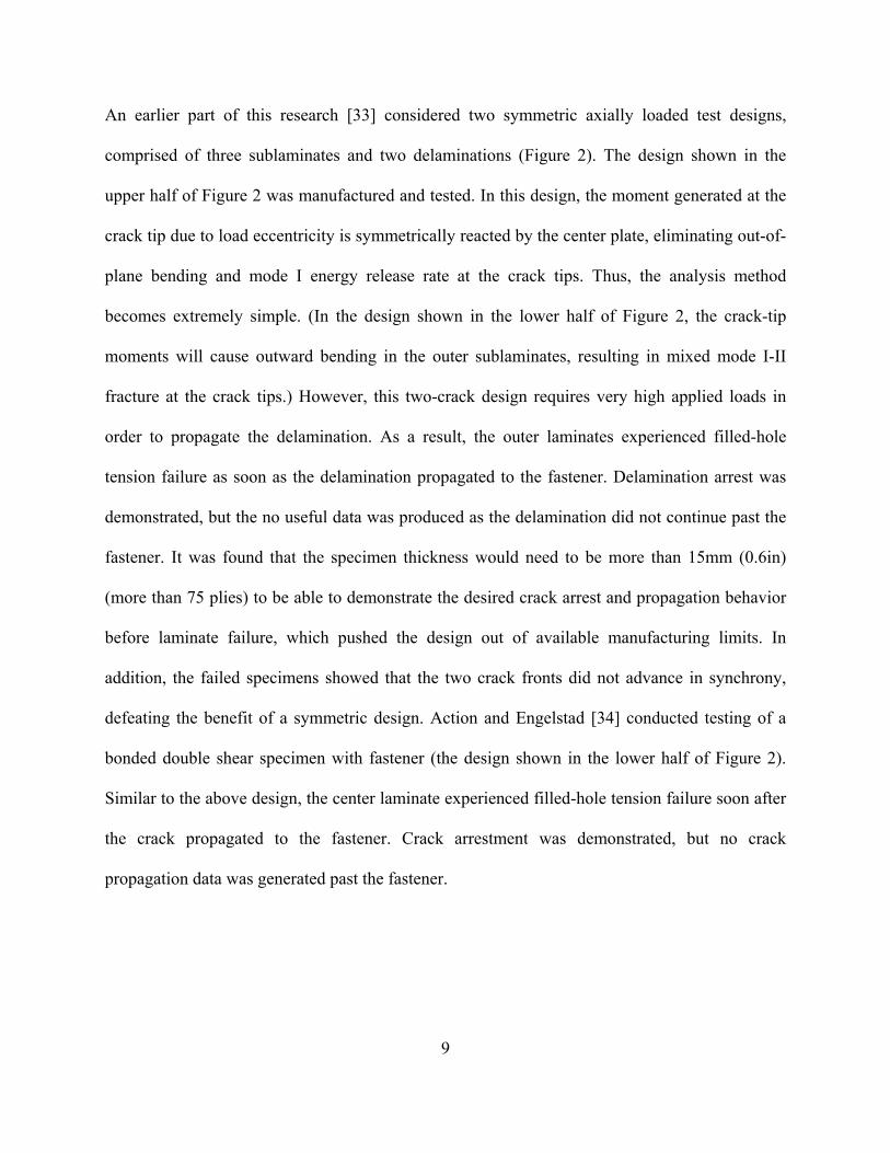
An earlier part of this research [33] considered two symmetric axially loaded test designs,
comprised of three sublaminates and two delaminations (Figure 2). The design shown in the
upper half of Figure 2 was manufactured and tested. In this design, the moment generated at the
crack tip due to load eccentricity is symmetrically reacted by the center plate, eliminating out-of-
plane bending and mode I energy release rate at the crack tips. Thus, the analysis method
becomes extremely simple. (In the design shown in the lower half of Figure 2, the crack-tip
moments will cause outward bending in the outer sublaminates, resulting in mixed mode I-II
fracture at the crack tips.) However, this two-crack design requires very high applied loads in
order to propagate the delamination. As a result, the outer laminates experienced filled-hole
tension failure as soon as the delamination propagated to the fastener. Delamination arrest was
demonstrated, but the no useful data was produced as the delamination did not continue past the
fastener. It was found that the specimen thickness would need to be more than 15mm (0.6in)
(more than 75 plies) to be able to demonstrate the desired crack arrest and propagation behavior
before laminate failure, which pushed the design out of available manufacturing limits. In
addition, the failed specimens showed that the two crack fronts did not advance in synchrony,
defeating the benefit of a symmetric design. Action and Engelstad [34] conducted testing of a
bonded double shear specimen with fastener (the design shown in the lower half of Figure 2).
Similar to the above design, the center laminate experienced filled-hole tension failure soon after
the crack propagated to the fastener. Crack arrestment was demonstrated, but no crack
propagation data was generated past the fastener.

10
Figure 2. Schematics of Symmetric Mode II Delamination Arrest Specimen Designs

11
Chapter 3. Finite Element Modeling
The purpose of the finite element analysis is to provide insights into the underlying mechanics of
mixed-mode crack propagation and using fastener as a crack arrest mechanism. The
understandings provided by the FEA were instrumental in the final design of the test and the
interpretation of the test results detailed in Chapter 5. The FE model was also used to verify the
analytical method detailed in Chapter 4.
A simplified 2-D model of a split-beam with a delamination arrest fastener, shown in Figure 3,
was used to evaluate the effectiveness of the fastener as a crack arrest mechanism. The split-
beam model is similar to that of a composite double cantilever beam (DCB), but with general
applied loads and moments. A fastener was added in front of the crack tip in the split-beam. The
change in crack propagation behavior before and after the crack encounters the fastener was
investigated.
The split-beam with fastener was modeled with finite elements and the crack propagation
behavior was numerically simulated in commercial finite element analysis software, Abaqus
[35]. Crack tip fracture was analyzed using the VCCT. The VCCT is a finite element
approximation of the modified crack closure technique, which calculates the mode-decomposed
crack tip strain energy release rates based on linear elastic fracture mechanics. The fastener was
modeled by two independent spring elements, one representing the axial stiffness of the fastener,
and the other representing the shear stiffness of the fastener shear joint. The stiffness of the shear
joint was calculated using the fastener flexibility approach by Huth.

12
The capability of the crack arrest fastener is measured in terms of the crack propagation load. For
unstable cracks, the crack propagation load would either decrease or remain the same as crack
length increases. This implies that a structure under load control would fail catastrophically as
soon as the critical propagation load is reached. For stable cracks, the crack propagation load
would increase as crack length increases. This increase in crack propagation load due to the
crack arrest fastener is the subject of this study.
The underlying mechanisms with which the fastener affects crack propagation are identified and
discussed later in this section.
3.1 Split-Beam Model Description
The finite element model used in this study is comprised of a lower beam, an upper beam and a
fastener (Figure 3). Identical, symmetric, balanced layups were used for both the upper and
lower beams to eliminate any crack-tip loading caused by thermal expansion and tension-
bending coupling. The layups used were (45/0/-45/90/45/0/-45/90)s and (45/02/-45/02/902)s,
representing 25% 0° plies (quasi-isotropic layup) and 50% 0° plies (high stiffness layup)
respectively. It is assumed that the crack is located at and confined to an infinitesimally thin
matrix interface between the upper and the lower beams. Fiber bridging and crack interface
migration are not considered. It is assumed that crack propagation occurs when the critical strain
energy rate is reached, regardless of bond type at the interface (co-cured, co-bonded or secondary
bonded) or fracture failure type (cohesive failure or adhesive failure). Their effects on the value
of the critical strain energy release rate are beyond the scope of this study.

13
Crack Interface and Propagation Direction
Initial Crack Tip Fastener
N1
M1
N2
M2
Lf = fastener location63.5mm (2.5in)
Lc = crack length50.8mm (2.0in)
Ltot = total length203.2mm (8.0in)
Lower plate (Beam 1)
Upper plate (Beam 2)3.048mm(0.12in)
Figure 3. Diagram of the Crack Arrest Finite Element Model
The model is 203.2mm (8.0in) in length and 31.75mm (1.25in) in width. The initial crack length
is 50.8mm (2.0in). The fastener springs are located 63.5mm (2.5in) from the cracked end. There
is 12.7mm (0.5in) space between the initial crack tip and the fastener. The crack propagation
between the initial crack tip and the fastener is not influenced by the fastener springs and is only
driven by the external loads. That is, the fastener is completely inactive between the crack-tip
location of 50.8mm (2.0in) and 63.5mm (2.5in). As the crack propagates past the fastener, the
fastener springs react to the crack opening and sliding displacements, and provide resistance to
propagation. Contact friction between the cracked surfaces is represented by specifying a
coefficient of friction for the interface.
14
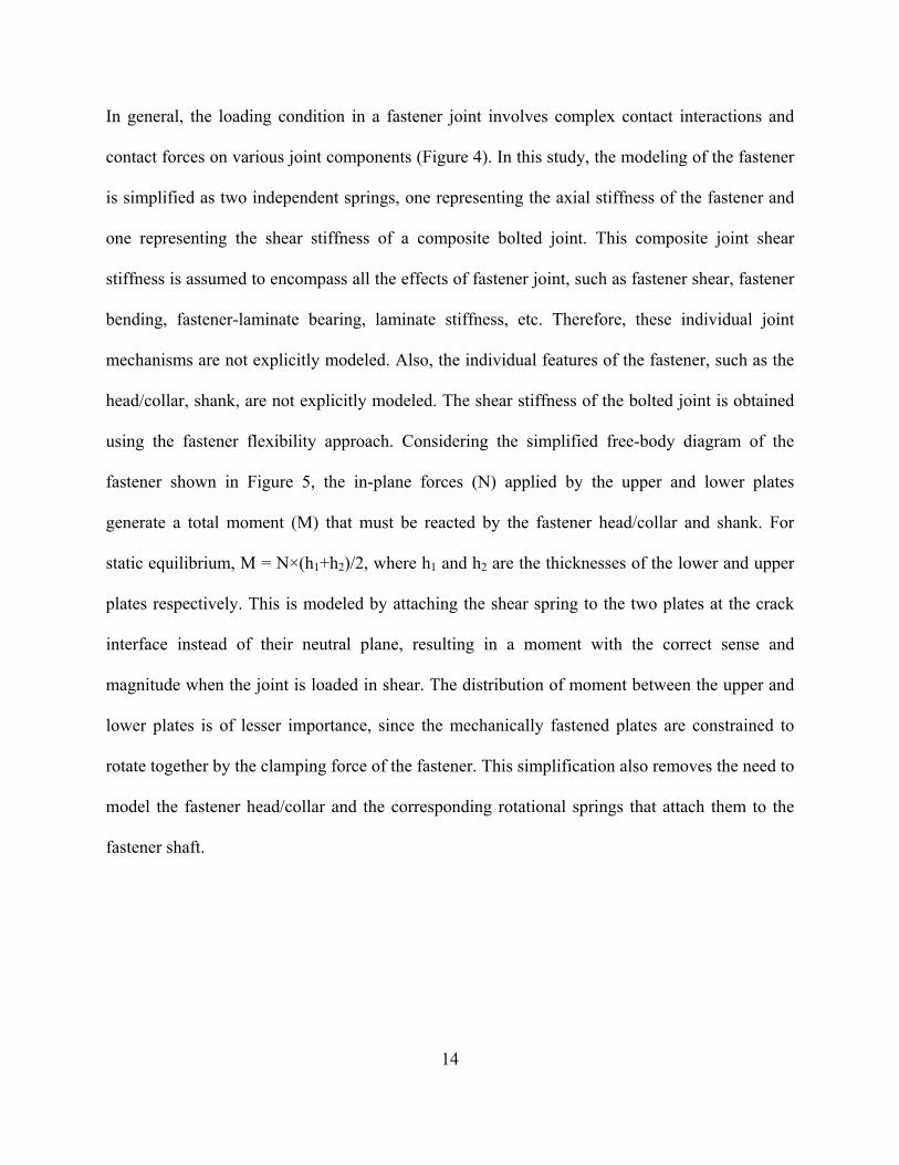
In general, the loading condition in a fastener joint involves complex contact interactions and
contact forces on various joint components (Figure 4). In this study, the modeling of the fastener
is simplified as two independent springs, one representing the axial stiffness of the fastener and
one representing the shear stiffness of a composite bolted joint. This composite joint shear
stiffness is assumed to encompass all the effects of fastener joint, such as fastener shear, fastener
bending, fastener-laminate bearing, laminate stiffness, etc. Therefore, these individual joint
mechanisms are not explicitly modeled. Also, the individual features of the fastener, such as the
head/collar, shank, are not explicitly modeled. The shear stiffness of the bolted joint is obtained
using the fastener flexibility approach. Considering the simplified free-body diagram of the
fastener shown in Figure 5, the in-plane forces (N) applied by the upper and lower plates
generate a total moment (M) that must be reacted by the fastener head/collar and shank. For
static equilibrium, M = N×(h1+h2)/2, where h1 and h2 are the thicknesses of the lower and upper
plates respectively. This is modeled by attaching the shear spring to the two plates at the crack
interface instead of their neutral plane, resulting in a moment with the correct sense and
magnitude when the joint is loaded in shear. The distribution of moment between the upper and
lower plates is of lesser importance, since the mechanically fastened plates are constrained to
rotate together by the clamping force of the fastener. This simplification also removes the need to
model the fastener head/collar and the corresponding rotational springs that attach them to the
fastener shaft.

15
Figure 4. Contact Forces in the Fastener and Plates in Single Shear
Figure 5. Net Forces and Moments in the Fastener in Single Shear
In this finite element study, only two load cases are considered. The first load case applies
symmetric opening moments to the two plates, resulting in pure mode I loading at the crack tip.
The second load case applies tension only to the lower plate, resulting in mixed-mode I/II
condition at the crack tip. The second load case is representative of a skin-stringer flange
termination, where the skin is loaded in tension and the flange termination is not loaded. These
load cases were chosen because they represent configurations that can be tested at a coupon
16
level. What is learned in the finite element analysis can be applied to the design of the test
specimen. The axial compression load case was not considered because it would result in pure
mode II crack tip loading (i.e. closing crack tip moment), which is less severe than mixed mode
I/II condition from the tension load case.
3.2 Material Properties
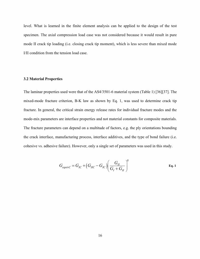
The laminar properties used were that of the AS4/3501-6 material system (Table 1) [36][37]. The
mixed-mode fracture criterion, B-K law as shown by Eq. 1, was used to determine crack tip
fracture. In general, the critical strain energy release rates for individual fracture modes and the
mode-mix parameters are interface properties and not material constants for composite materials.
The fracture parameters can depend on a multitude of factors, e.g. the ply orientations bounding
the crack interface, manufacturing process, interface additives, and the type of bond failure (i.e.
cohesive vs. adhesive failure). However, only a single set of parameters was used in this study.
IIequivC IC IIC IC
I II
GG G G G
G G
Eq. 1

17
Table 1. Carbon Fiber Reinforced Plastic Laminar Material Properties (AS4/3501-6)
SI Units English Units
Ply thickness 0.1905 mm 0.0075 in
E1 127.5 GPa 18.5 Msi
E2 = E3 11.3 GPa 1.64 Msi
G12 = G13 6.0 GPa 0.871 Msi
G23 3.6 GPa 0.522 Msi
ν12 = ν13 0.3
ν23 0.4
GIC 262.7 J/m2 1.5 in-lb/in2
GIIC 1226 J/m2 7.0 in-lb/in2
η 1.75
A Titanium fastener (typically of the material Ti-Al6-V4) with an elastic modulus of 113.8GPa
(16.5Msi) was used. The stiffness of the fastener axial spring was as calculated as a constant
diameter rod, k = A×E/(t1+t2). The stiffness of the fastener shear spring was calculated using the
fastener flexibility approach. The flexibility of the un-bonded bolted joint in the shear direction,
C, is given by Eq. 2. The parameters used are: ti = laminate thickness, d = fastener diameter, n =
single or double shear joint, E1 = E2 = laminate stiffness, Ef = fastener elastic modulus, constants
a = 2/3 and b = 4.2 for bolted graphite/epoxy joints. A force offset at zero spring elongation was
added to the fastener axial spring to simulate fastener preload (Figure 6). The effect of contact
coefficient of friction was also studied.

18
1 2
1 1 2 2 1 2
1 1 1 12 2 2
a
f f
t t bCd n t E nt E t E nt E
Eq. 2
Figure 6. Spring Load-Displacement Curve for Fastener with Preload
The properties of the materials and structural members were assumed to be linear elastic. The
only failure considered in the finite element analysis was crack tip fracture and propagation.
Alternate failure modes, such as laminate failure, fastener failure and bearing failure, were not
considered in this study. These competing failure modes would provide realistic constraints for
the design and optimization of the crack arrest feature, but was not the primary focus of this
study.

3.3 The F
The 2-D
software
of a DCB
beams ar
element
element a
in order t
and behin
The faste
surfaces
propertie
F
Finite Elem
D finite elem
(Version 6.
B except for
re identical
with reduce
aspect ratio
to maintain
nd the crack
ener axial sp
of the DCB.
es, such that
Figure 7. Finit
ment Model
ment model
12-1), as sho
the addition
separate pa
ed integratio
kept close to
the self-sim
k tip are not t
pring elemen
. Fastener pr
the spring is
te Element Me
was constr
own in Figu
n of the two f
rts. The CP
on is used. E
o one. The e
milar conditio
the same, the
nt (Abaqus
reload is mod
s in tension a
esh of the Spli
19
ructed using
ure 7 and Fig
fastener spri
PEG4 2-D 4
Each ply th
element size
on required f
e energy rele
“spring2” e
deled by pro
at zero displa
it-Beam Mode
g Abaqus/C
gure 8 [38].
ings and load
-node biline
hickness is r
e is uniform
for VCCT. I
ease rate calc
element) is c
oviding the s
acement.
el (Deformed u
CAE finite
The mesh is
d cases. The
ear quadrilat
represented
along the le
If element le
culation can
connected to
spring eleme
under Mode I
element ana
s identical to
e upper and l
teral plane s
by one elem
ength of the b
engths in fro
n be inaccura
o top and bo
ent with nonl
I Loading)
alysis
o that
lower
strain
ment,
beam
ont of
ate.
ottom
linear

The uppe
interactio
while the
crack tip
SERR fo
displacem
when the
next nod
contact f
definition
regardles
Figure 8. Fin
er and lower
on definition
e cracked su
, the mode-d
or each mod
ments behind
e mixed-mod
de. As the no
friction is mo
n. The crac
ss of the stab
nite Element M
r beams are
n in Abaqus.
urfaces beha
decomposed
de is calcula
d the crack
de fracture fa
ode at the cr
odeled by pr
ck propagat
bility of the
Mesh of the Sp
bonded to e
The nodes a
ave as free s
d SERRs are
ated separat
tip. The tie
ailure criteri
ack tip is re
roviding coe
es in the f
propagation
20
plit-Beam Mo
each other al
along the int
surfaces with
e evaluated u
ely using th
condition ap
ion (Eq. 1) is
leased, a new
efficients of
finite eleme
n. For examp
odel (Enlarged
long their in
tact portion o
h contact an
using the Ab
he nodal for
applied to th
s met, and th
w cracked s
friction to th
ent analysis
ple, if crack
d Near the Cra
nterface usin
of the beam
nd friction r
baqus VCCT
rces and the
he crack tip n
he crack tip
surface is cre
the VCCT su
in a node
propagation
ack Tip)
ng VCCT su
are tied toge
resolution. A
T algorithm
e opening/sl
nodes is rele
propagates t
eated. Crack
urface intera
-to-node fa
n is unstable
urface
ether,
At the
m. The
liding
eased
to the
k-face
action
shion
e with

21
respect to the load/boundary applied, multiple nodes will sequentially release while the applied
load/boundary remains constant.
The crack propagation analysis consists of many individual static equilibrium steps, one for each
crack tip node release. Essentially, each time the crack propagates forward, a new structure is
created and the static analysis is repeated. A large number of iterations are required to resolve
crack-face contact and contact friction forces. Solution convergence is difficult due to the
instabilities that arise when crack propagation results in a sudden drop in stiffness of the
structure. Automatic damping was used in Abaqus to aid convergence. The amount of damping
was minimized such that it made no significant impact on the solution. Thermal contraction due
to curing was not simulated because the two beams are identical with symmetric and balanced
layup (strain energy release rates are not induced by changing temperature).
3.4 Results and Discussions
This study was structured to analyze the behaviors of a delamination arrest fastener feature in
progressive complexity. The baseline configuration is a split-beam under mode I and mode II
loadings. First, a fastener with no preload was added to the model. Then, crack-face friction and
fastener preload were modeled to simulate the realistic install condition of fasteners. The goal is
to obtain a comprehensive understanding of how the fastener arrested crack propagation and to
identify individual mechanisms that contributed to the efficacy of the crack arrest fastener. The
emphasis of this section is on the qualitative understanding of the arrestment feature, which is

22
used to guide the development of the analytical method and the test design detailed in Chapter 4
and Chapter 5.
3.4.1 Effect of Fastener under Mode I Loading
Mode I interlaminar fracture in composites is generally the most critical fracture mode because
GIC is much lower than GIIC (and GIIIC). The opening mode also allows moisture and
contaminants to seep into the cracked surface, exacerbating the damage over cycling mechanical
and thermal loading. The mechanics of crack arrest with a fastener under mode I loading is well
understood. The finite element analyses of pure mode I loading and crack arrestment are
discussed here as one of the most important part of the fastener arrest mechanism.
Figure 9 shows the applied moment vs. crack-tip location for the 25%-0° and 50%-0° lay-ups
with and without an arrest fastener. The fastener is positioned at crack location zero. Without the
fastener, the crack propagation is neutrally unstable, as shown by the horizontal lines in the
figure. This occurs because the applied moments produce a constant GI at the crack tip that is
independent of crack length, thus crack propagation is catastrophic once the critical moment is
reached. When a fastener is included in the model, it is clear that the crack is effectively arrested,
as shown by the rising curves in the figure. This is expected since the axial stiffness of the
fastener mechanically prevents the crack tip from opening, thus completely eliminating mode I
propagation. The crack stops well within the diameter of the fastener. The crack is completely
arrested because the pivot provided by the fastener results in a closing moment at the crack tip as
the applied opening moment increases. The change in the axial stiffness of the lay-up does not

23
have any noticeable impact on the arrest effectiveness of the fastener. It is also observed that the
required moment increased slightly before the crack tip reached the fastener location. This is
because the beam bending is causing deflection at the fastener even before the crack tip reaches
the fastener. For an explicit fastener, crack propagation will be arrested at the edge of the
fastener head/collar and washer. Although not modeled in the finite element analysis, the
ultimate failure mode under mode I loading will likely be laminate failure in bending, fastener
failure in tension (e.g. net section failure, head/collar failure), or fastener pull-through.
Figure 9. Propagation Moment vs. Crack-Tip Location in Mode I
0
20
40
60
80
100
‐1.5 ‐1 ‐0.5 0 0.5 1 1.5
Applied M
oment (N‐m
)
Crack‐Tip Location (mm)
25% 0‐deg
50% 0‐deg
25% 0‐deg no fastener
50% 0‐deg no fastener

24
3.4.2 Effect of Fastener under Mixed-Mode Loading
In general, composite structures experience mixed mode I and II loading conditions at the
delamination interface. Under tension, load path eccentricity produces a secondary moment that
opens the crack tip. The presence of even a small amount of GI could greatly reduce the
capability of the structure to resist crack propagation. Such configuration can be found when a
stringer flange terminates on a skin under tension. Under compression, the secondary moment is
in the closing direction. Therefore, compression is generally considered a less critical load case.
Figure 10. Deformation of a DCB with Fastener with Applied Tension on the Lower Beam
The effectiveness of the fastener under mixed-mode load case was investigated. The mixed-
mode crack tip condition is created by applying axial tension to only the lower beam (Figure 10).
It should be noted that due to the finite dimensions of the FE model and large beam-column
deformations, while the external load case remained the same, the fracture mode-mixity would
change slightly as the crack propagated across the model. Figure 11 shows the applied tension
load vs. crack-tip location for the 25%-0° and 50%-0° lay-ups with and without a fastener. The

25
crack propagation is only marginally stable without a fastener, as shown by the nearly horizontal
curves. (The lines terminated because the solver failed to converge when crack propagation
became unstable.) The critical loads for the 25%-0° and 50%-0° lay-ups are 24.9kN (5.6kips)
and 28.9kN (6.5kips), respectively. With a fastener, the propagation load increases drastically, as
shown by the curves with step increases in propagation loads. The propagation loads for the
25%-0° and 50%-0° lay-ups jump to 35.6kN (8.0kips) and 42.0kN (9.4kips), respectively, at the
crack-tip location of 5mm (0.2in). This represents a 42% and 45% increase over the critical loads
without a fastener. After the crack tip exits the fastener location, crack propagation continues in a
stable fashion. In the mixed-mode load case, the propagation load increases in two different
stages: a step jump in the immediate vicinity of the fastener, and a gradual increase after the
crack tip propagated past the fastener. It is crucial to note that the crack tip is no longer
completely arrested under this load case, but is retarded by the fastener shear joint stiffness. This
observation is drastically different from that of the pure mode I load case discussed in Chapter
3.4.1.
The behavior of the load vs. crack-tip location curves in Figure 11 implies that two different
mechanisms are acting together to provide overall the arrest capability. Figure 12, which shows
the SERR components required for propagation vs. crack-tip location, effectively illustrates the
first mechanism at work – mode I suppression. As the crack propagates past the fastener, the
fastener axial stiffness prevents the crack-tip from opening. As a result, the mode I strain energy
release rate, GI, drops to zero. This forces the crack to propagate in pure mode II. This can only
be achieved by increasing the applied load significantly (as shown by the step jumps in
propagation loads in Figure 11), driving the mode II strain energy release rate, GII, up to GIIC in
order to make up for the loss in GI. Mode I suppression is effective in providing a large step

26
increase in the propagation load as the crack reaches the fastener. The crack appears to be
“temporarily arrested.” The benefit of suppression is also dependent on the amount of GI present
before the crack tip reaches the fastener. If crack propagation is in pure mode II, this mechanism
will provide no benefit to crack arrestment and no step increase in propagation load can be
observed.
Figure 11. Propagation Load vs. Crack-Tip Location in Mixed-Mode
0
10
20
30
40
50
60
‐10 0 10 20 30 40 50 60 70 80 90
Axial Load
(kN
)
Crack‐Tip Location (mm)
25% 0‐deg
50% 0‐deg
25% 0‐deg no fastener
50% 0‐deg no fastener

27
Figure 12. SERR Components Required for Propagation vs. Crack-Tip Location in Mixed-Mode
The second mechanism is the resistance provided by the fastener joint shear stiffness (i.e.
fastener flexibility). As the crack separates the intact portion of the beam, the newly formed sub-
laminates and the fastener form a fastener joint. The fastener transfers some of the axial load and
reduces the loading at the crack tip. The percentage of load transferred by the fastener increases
as the crack tip advances, thus providing increasing resistance to crack propagation. As a result,
crack propagation beyond the fastener remains stable, requiring higher load for further crack
growth. The propagation stability provided by the fastener is primarily driven by factors that
impact the fastener flexibility, such as laminate stiffness, laminate thickness, fastener stiffness,
0
200
400
600
800
1000
1200
1400
‐10 ‐5 0 5 10
SERR (J/m^2)
Crack‐Tip Location (mm)
GI
GII
GI no fastener
GII no fastener

28
and fastener diameter. In general, the stiffer the fastener joint, the more stability is added, and the
slope of the load vs. crack-tip location curve is higher. Although crack propagation is stable, the
arresting effect is greatly diminished comparing to mode I suppression. In this regime, crack
propagation is retarded, not arrested. Once the crack propagates past the fastener, a relatively
small increase in apply load would cause significant crack growth.
3.4.3 Effect of Contact Friction and Fastener Preload under Mixed-Mode Loading
Crack-face friction has been a persistent issue in specimens designed to measure the mode II
critical strain energy release rate (GIIC), such as the ENF specimen. The contact friction behind
the crack tip inflates the load required to cause crack propagation, thus leads to inaccurate
measurement of GIIC. However, crack-face friction plays an important and beneficial role in the
crack arrest fastener. The friction of interest is generated by the fastener preload (clamp up), and
therefore only acts in the vicinity of the fastener. Fastener preloads in structural assemblies often
approach the tensile yield strength of the fastener, resulting in friction forces that are orders of
magnitude greater than that between an unfastened surface pair (e.g. the ENF). Therefore, the
analysis model must include a realistic portrayal of fastener preload and friction.
To study the effect of friction, the mixed-mode load case used in Chapter 3.4.2 was applied to
the split-beam with 25% 0-deg layup. A constant fastener preload of 16.4kN (3680lb; 50% of a
6.35mm / 0.25in fastener tensile yield strength) was applied. Typically, a newly installed fastener
would have preload of around 80% of its tensile yield strength, a lower value of 50% was used to

29
simulate the through-thickness visco-elastic relaxation of the composite laminate. The crack-face
static coefficient of friction (μ) was varied from zero to 0.75.
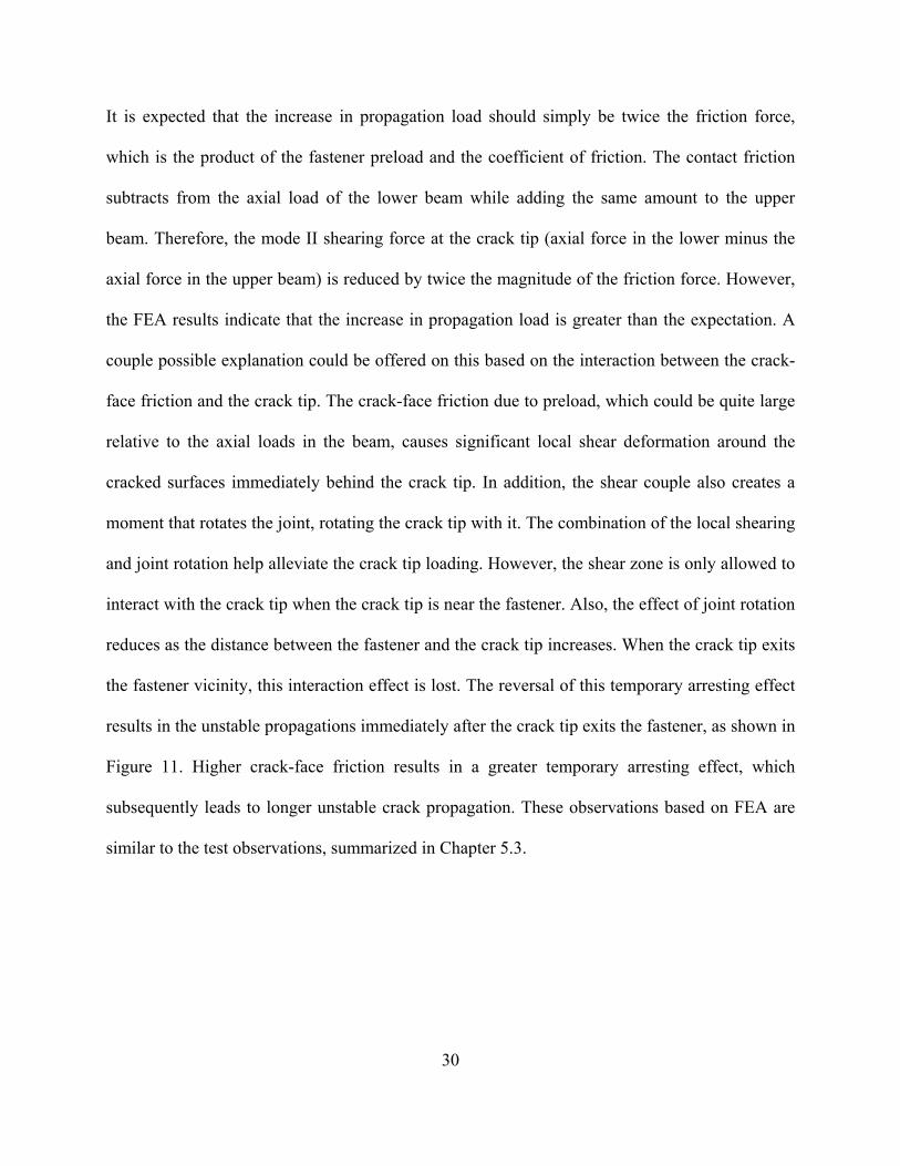
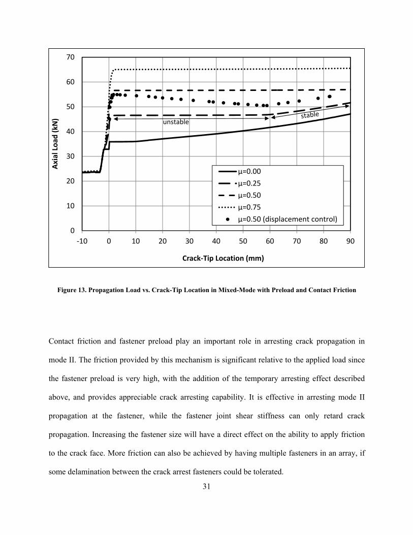
Figure 13 shows the applied tension load vs. crack-tip location under the above conditions. The
curve for the frictionless case is almost the same as the corresponding curve in Figure 11. The
jump in propagation load due to mode I suppression occurs slightly before the crack tip reaches
the fastener. This is due to the extended influence of the fastener generated by the preload. The
peak of the propagation load jump increases in proportion to the coefficient of friction. The load
peaks reach 32.9kN, 46.3kN, 55.2kN, and 63.2kN (7.4kips, 10.4kips, 12.4kips, and 14.2kips) for
μ of 0, 0.25, 0.5, and 0.75, respectively. As the crack tip propagates toward the fastener, new
cracked surfaces are created and crack-face friction builds up behind the crack tip. The friction
reduces the force available at the crack tip, leading to the step increases in the propagation load.
After the initial jump, the propagation load does not increase smoothly for the cases with non-
zero friction. Instead, there are large segments of unstable crack propagations as the crack tip
exits the fastener region. For example, in the case where μ=0.25, the crack tip remains at 1mm
(0.04in) up to 46kN (10.3kips), but propagates to 60mm (2.4in) as soon as the load exceeds
45.8kN (10.3kips). The length of the unstable propagation increases with the coefficient of
friction. A displacement control analysis was repeated for the μ=0.5 case, the result shows that
the propagation load decreases steadily during the unstable propagation despite the stabilizing
effect of the fastener shear joint. The propagation load begins to recover after the crack tip
reached a location of 60mm (2.4in). This implies that the crack tip driving force is increasing as
the crack tip exits the fastener area, while the applied load remains the same.
30
It is expected that the increase in propagation load should simply be twice the friction force,
which is the product of the fastener preload and the coefficient of friction. The contact friction
subtracts from the axial load of the lower beam while adding the same amount to the upper
beam. Therefore, the mode II shearing force at the crack tip (axial force in the lower minus the
axial force in the upper beam) is reduced by twice the magnitude of the friction force. However,
the FEA results indicate that the increase in propagation load is greater than the expectation. A
couple possible explanation could be offered on this based on the interaction between the crack-
face friction and the crack tip. The crack-face friction due to preload, which could be quite large
relative to the axial loads in the beam, causes significant local shear deformation around the
cracked surfaces immediately behind the crack tip. In addition, the shear couple also creates a
moment that rotates the joint, rotating the crack tip with it. The combination of the local shearing
and joint rotation help alleviate the crack tip loading. However, the shear zone is only allowed to
interact with the crack tip when the crack tip is near the fastener. Also, the effect of joint rotation
reduces as the distance between the fastener and the crack tip increases. When the crack tip exits
the fastener vicinity, this interaction effect is lost. The reversal of this temporary arresting effect
results in the unstable propagations immediately after the crack tip exits the fastener, as shown in
Figure 11. Higher crack-face friction results in a greater temporary arresting effect, which
subsequently leads to longer unstable crack propagation. These observations based on FEA are
similar to the test observations, summarized in Chapter 5.3.
31
Figure 13. Propagation Load vs. Crack-Tip Location in Mixed-Mode with Preload and Contact Friction
Contact friction and fastener preload play an important role in arresting crack propagation in
mode II. The friction provided by this mechanism is significant relative to the applied load since
the fastener preload is very high, with the addition of the temporary arresting effect described
above, and provides appreciable crack arresting capability. It is effective in arresting mode II
propagation at the fastener, while the fastener joint shear stiffness can only retard crack
propagation. Increasing the fastener size will have a direct effect on the ability to apply friction
to the crack face. More friction can also be achieved by having multiple fasteners in an array, if
some delamination between the crack arrest fasteners could be tolerated.
0
10
20
30
40
50
60
70
‐10 0 10 20 30 40 50 60 70 80 90
Axial Load
(kN
)
Crack‐Tip Location (mm)
μ=0.00
μ=0.25
μ=0.50
μ=0.75
µ=0.50 (displacement control)
unstable

32
It is important to note that fastener with preload can apply large friction forces on the cracked
surfaces, while other arrest features such as z-stitch (through thread pre-tension) and z-pins
(through thermal residual stresses) cannot deliver large through-thickness compression. This
effect is significant because mechanical fastener with high preload can generate friction force
that is comparable to the in-plane loads in the laminates. A significant portion of the total crack
arrest capability can be attributed to friction.
3.4.4 Discussion of the Main Crack Arrest Mechanisms
The analysis results in Chapters 3.4.1 to 3.4.3 illustrate three key mechanisms with which a
fastener provides crack arrestment capability. The three mechanisms are identified as 1) mode I
suppression by fastener axial stiffness, 2) crack-face friction from fastener preload, and 3) load
transfer by fastener joint shear stiffness.
Mode I suppression works by mechanically closing the crack tip, thus eliminating the mode I
component of a normally mixed-mode crack, forcing the crack to propagate in pure mode II.
This requires additional loads to drive up GII to make up for the loss in GI, arresting the crack
propagation in the meantime. This mechanism is effective specifically for laminated composites
because of their very low mode I critical strain energy release rates (GIC) and much higher mode
II critical strain energy release rates (GIIC). In addition, the crack tip is effectively arrested at the
fastener location without overrunning the feature. However, the apparent benefit depends on the
mode mixity, the ratio of mode I to mode II, of the crack tip and the load case. If crack
propagation is pure mode I, the fastener can completely stop the crack. If crack propagation is
pure mode II, no benefit can be realized from eliminating the mode I fracture component.

33
Alternate delamination arrestment features, such as z-pin and stitching, operate under the same
principle, but in a more distributed fashion.
Crack-face friction from fastener preload works by generating a large amount of friction under
the fastener, thus resisting mode II crack propagation. The friction force is very high because the
fastener preload can be greater than 50% of the fastener tensile yield strength for a properly
installed fastener. In addition, the apparent benefit of friction is greater when the surface traction
interacts with the crack tip in close proximity. However, this effect reverts itself when the crack
tip exits the fastener are, leading to unstable crack propagations. Similar to mode I suppression,
most of the benefit from crack-face friction is realized when the crack tip is directly underneath
the fastener, before it is allowed overrun the feature. Fasteners have the greatest advantage
because of their high preload. Alternatives such as pre-stressed stitches can provide smaller and
distributed through thickness compression, while z-pins provide no benefit. However, the
coefficient of friction of the cracked surfaces is difficult to quantify and could decrease if the
surfaces are allowed to wear out under cyclic loading. Also, the magnitude of fastener preload
has high variability and is highly dependent on the installation process.
Fastener joint shear stiffness works by providing elastic resistance to mode II propagation that
retards crack propagation. The fastener shear joint provides a load transfer path around the crack
tip, thus reducing the crack-tip forces and moments. The percentage of load transfer increases as
the crack length increases. The retarding effect of joint stiffness is mild, but it stabilizes crack
propagation beyond the fastener and prevents catastrophic breakup of the structure. Unlike mode
I suppression and crack-face friction, which are effective in arresting the crack at the fastener
location, fastener joint stiffness only provides resistance to propagation after the crack tip has

34
past the fastener. Therefore, this is only a crack retardation mechanism. In addition, composite
fastener joints tend to be more flexible and are installed with positive fit clearance, making them
less effective in resisting crack propagation.
3.4.5 Alternate Failure Modes not Considered in the Current Analysis
The finite element analysis discussed in this section focuses primarily on the interlaminar
fracture of the composite laminate and the behavior of the crack arrest fastener. Alternate failure
modes were not simulated. These alternate failure modes include in-plane (e.g. filled/open-hole
tension) and bending failure of the laminate, fastener shear and tension failure (e.g. tensile/shear
yield, head pop off), laminate bearing failure, and fastener head pull-through.
Typically, the interlaminar failure load is much lower than the laminate in-plane failure modes.
The crack arrest fastener should be designed such that its capability meets or exceeds the failure
load of the most critical laminate failure mode. This way, the strength capability of the laminate
can be efficiently utilized. Here, the capability of the delamination arrest fastener is loosely
defined, as it also depends on the acceptable crack propagation beyond the fastener. However,
allowing crack propagation beyond the arrest feature adds a lot of difficulties in design and
analysis. Once the crack tip overruns a fastener, a new bolted joint is created. Analysis must be
conducted on this new detail, which requires developing new loads and performing margins
checks for all pertinent failure modes and load cases. Also, allowing the crack to overrun an
arrest feature also jeopardizes substantiation to the FAR 23.573 bonded joint requirement.
Therefore, one possible approach would be to define the arrest capability as the peak load before

35
the crack tip exits the fastener area. This definition ensures that the crack is arrested at the
fastener location, simplifying the analysis of the structure in all other failure modes.

36
Chapter 4. Development of the Analytical Method
An analytical solution was developed to model the delamination arrest fastener problem with
capabilities comparable to the finite element method. The costly through-thickness modeling
with plane strain finite elements was replaced with an idealized beam-column model. The
analytical solution is based on the principle of minimum potential energy (PMPE) using the
Rayleigh-Ritz solution method, which is sufficiently robust for most configurations and load
cases. Crack tip strain energy release rates are calculated using Davidson’s crack-tip element.
The goal is to develop an analytical method that is computationally efficient for large-volume
applications, such as parametric/sensitivity studies, design optimization, and probabilistic
analysis.
This section is divided into four parts. Part one describes the analytical model and modeling
assumptions. Part two explains the solution method, which employed the Rayleigh-Ritz method
to determine the static equilibrium of the model. Part three outlines the numerical
implementation of the solution in MATLAB. Part four compares the solutions of the analytical
model to that of the finite element model.
4.1 Analytical Model and Modeling Assumptions
The analytical model resembles the split-beam configuration of the FE model (Figure 14). The
model simulates the crack propagation behavior in a split-beam by dividing it into cracked and
non-cracked segments. The non-cracked beam between the fixed boundary and the crack tip is

37
referred to as the “intact segment.” The cracked beams between the crack tip and the fastener are
referred to the “cracked segments.” Crack length of interest is defined as the distance from the
crack tip to the fastener only, or crack-tip location with respect to the fastener. The cracked
beams between the fastener and the far-field, where loads and moments are applied, are referred
to as the “freed segments.” Segmentation of the model is necessary because the crack tip and the
fastener represent discontinuities in the structure; hence, the behavior of each beam cannot be
described using a single displacement function. For identification purposes, the upper beam is
referred as “beam 1” and the lower beam is “beam 2.”
Figure 14. Schematic of Analytical Model
The model is decomposed into a total of five beam-column elements. The fastener is idealized as
two springs, one representing the fastener axial stiffness and one representing the joint shear
stiffness. They are attached to the junctions between the cracked beam segments and the freed

38
beam segments. Figure 15 and Figure 16 provide a simplified depiction of the connection and
interaction between these beam-column elements and springs in deflection and axial
displacement. The orientation used is such that positive x-direction is to the right, and positive z-
direction is to the top. The forces and moments sign convention are such that positive axial load
(N) results in axial tension or positive x-displacement, and positive moment (M) creates clock-
wise bending or deflection in the negative z-direction.
Figure 15. Beam-Column Model – Bending Deflection and Interactions in the Z-Direction
Figure 16. Beam-Column Model – Axial Extension and Interactions in the X-Direction

39
The details of the beam-column connectivity are discussed here. The intact beam, representing
the full-thickness of the laminate, is given fixed boundary conditions at the left end. Zero x-z
displacements and slope are enforced. The left ends of the cracked segments of beam 1 and beam
2 are attached to the right end of the intact beam. The attachment is accomplished by using stiff
springs (k∞) that enforce equal x-z displacements and slope at the connection. The freed
segments of beam 1 and beam 2 are attached to the cracked segments of beam 1 and beam 2,
respectively, using stiff springs. Although the freed segments are not directly involved in the
simulation of crack propagation, they are needed to resolve the beam-column effect between the
fastener and the far field boundary conditions. Contact springs in the z-direction are distributed
along the length of the cracked and freed segments of the beams to resolve contact interactions
and forces. The contact spring is either stiff or has zero stiffness depending on its contact state.
The individual contact spring is activated when local penetration between beam 1 and beam 2 is
detected. The on/off states of the contact springs must be determined iteratively. Friction
between the cracked beams due to contact normal forces are not modeled because it is negligible
compared to the friction force generated by fastener preload. Friction generated by fastener
preload, which is technically also contact normal force but only occurs at the fastener location, is
accounted for in the fastener joint modeling.
The fastener is modeled as two springs representing the fastener axial stiffness and the joint
shear stiffness. The fastener axial stiffness is given by A×E/(h1+h2). The joint shear stiffness is
obtained using the fastener flexibility approach. The sense and the magnitude of the joint
moment can be correctly modeled by attaching the springs to the lower surface of beam 1 and the
upper surface of beam 2. As such, the sliding displacement that determines the joint load is
calculated at the crack interface, not at the mid-plane of the cracked beams.
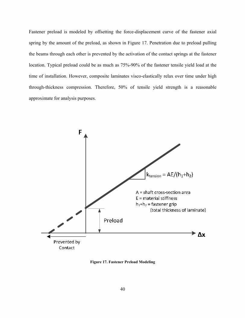
40
Fastener preload is modeled by offsetting the force-displacement curve of the fastener axial
spring by the amount of the preload, as shown in Figure 17. Penetration due to preload pulling
the beams through each other is prevented by the activation of the contact springs at the fastener
location. Typical preload could be as much as 75%-90% of the fastener tensile yield load at the
time of installation. However, composite laminates visco-elastically relax over time under high
through-thickness compression. Therefore, 50% of tensile yield strength is a reasonable
approximate for analysis purposes.
Figure 17. Fastener Preload Modeling

41
The effects of crack-face friction generated by the fastener preload and the effect of fastener hole
clearance are modeled using a nonlinear force-displacement curve for the joint shear spring, as
shown in Figure 18. The nominal fastener joint stiffness is assumed linear and is calculated using
fastener flexibility approach. The fastener hole clearance is given as a constant amount of
displacement, usually as a manufacturing/assembly specification. The fastener joint does not
transfer shear load through the fastener shaft unless the sliding displacement exceeds the hole
clearance. The crack-face friction is calculated as the product of the fastener preload and a crack-
face coefficient of friction [39]. A “pristine interface” coefficient of friction should be used to
represent structures in static tests; while a “worn out” coefficient of friction should be used to
simulate the effect of crack-face wearing under cyclic loads. If the load transferred through the
joint is at or below the friction limit, the cracked surfaces are locked. Joint total shear load and
moment are non-zero, but the sliding displacement and the load transferred through the shaft is
zero. In this regime, the joint shear stiffness is assumed to be infinite. When the load transferred
through the joint exceeds the friction limit, the joint must first slips for the amount equal to the
fastener hole clearance (i.e. the horizontal segment in Figure 18) without additional resistance.
The slip does not stop midway on the horizontal line because the joint will slide all the way to
the knee of the curve as soon as slipping occurs. The slip is arrested when the fastener shaft
engages the hole and begins to transfer load via fastener bolt shear, after which the joint behaves
linearly. It should be noted that when the friction exceeds the surface shear strength of the
exposed matrix on the cracked surfaces, the matrix will fail and the cracked surfaces will begin
to abrade. For simplicity, cracked surface abrasion is not modeled.

42
Figure 18. Fastener Shear Joint with Friction and Hole Clearance Modeling
A few simplifications, idealizations and assumptions were made as part of the analytical model.
A short summary is provided below.
The use of Rayleigh-Ritz method and predefined displacement functions mean that the
solution obtained is an approximation of the actual solution. Similarly, the contact
resolution algorithm can only provide an approximate solution of the contact state. It is
possible to have non-convergence due to contact “chattering,” partly due to the artificial
stiffness assumed between the beams.
The beam material and fastener material properties are assumed to be linear. The
assumption that the laminate elastic properties are linear to failure is valid in most

43
circumstances, as long as there is no additional damage other than the primary
delamination. The fastener joint shear stiffness is assumed to be linear for simplicity
(except for the modeling of friction and hole clearance). While this assumption is
generally good for low load/strain scenarios, it is reasonable to expect nonlinearities at
high loads due to fastener hole elongation and local bearing crushing. The nonlinear joint
behavior is evident in the data presented in Huth’s fastener flexibility study.
The laminates are modeled using classical beam-columns, i.e. zeroth order or shear non-
deformable. Transverse shear deformation is neglected. Inaccuracies might arise in
scenarios where transverse shear and shear lag effects are large compared to beam
bending deformation. In addition, local transverse shear can directly interact with the
crack tip, which cannot be captured in the current beam-column and crack-tip element
model. The use of the plane strain formulation implies that the laminate has no
strain/curvature in the depth dimension (y-direction).
4.2 Solution Method: Rayleigh-Ritz Method (PMPE)
The principle of minimum potential energy is used to determine the static equilibrium of the
beam-fastener system. The principle states that the total potential energy (Π) expressed as a
function of the displacement, attains a minimum value at the correct displacement. At the
minimum energy state, the variation of Π with respect to displacement is zero, or δ(Π)=0, where
δ is a small variation. The total potential energy can be expressed as the strain energy (U) less the
work potential (W). The PMPE can be written as Eq. 3.

44
0U W Eq. 3
In practice, PMPE is used to obtain an approximation of the exact solution, because the
analytical description of the exact displacement field is unavailable a priori, or infeasible to
compute. Therefore, assumed shape functions are used to approximate the exact displacements of
the system, from which the best-estimate solution is obtained. However, with a well understood
system, well-selected generic shape functions with enough higher order terms satisfying
completeness can provide a solution with sufficient accuracy. In this study, 6th degree
polynomials and 2nd degree polynomials are used as shape functions for the out-of-plane
displacement and axial displacement, respectively.
The Rayleigh-Ritz method is employed to determine the approximate solution of the system
based on the principle of minimum potential energy. The displacements of the system are
expressed as a linear superposition of N unknown coefficients, θn, multiplied by n known
assumed shape functions, fn(x), which must satisfy the geometric boundary conditions.
Expressions for the strain energy and the work potential are obtained based on the assumed
shape functions. As a result, the total potential energy in the structure can be expressed in terms
of the n coefficients that determine the displacements. The solution can be obtained by finding
the θn’s such that Π is minimized; this is equivalent to a linear n-dimensional optimization
problem. Since the system is linear, the gradient of Π with respect to θn’s can be written as a set
of N linear equations shown in Eq. 4. Solving the set of linear algebraic equations yields the
approximate displacement solution for the system. Here, since the model is nonlinear due to
contact interactions, friction, and hole clearance, a “guess solution” is obtained each time the set
of linear equations are solved. The converged solution is found using an iterative process.

45
0 ,where 1...n
n N
Eq. 4
First, the displacement shape functions are established for the beam-column elements in the
model. Simple polynomials are used because they satisfy the geometric boundary conditions and
are well-behaved with localized contacts (trigonometric series were found to be not suitable with
contact modeling due to the undulating nature of the functions). The general form for out-of-
plane deflection at the mid-plane of the beam-column is given by Eq. 5, where the deflection of
the ith beam as a function of x, wi(x), is expressed as a polynomial of degree j. The unknown
coefficients βi,j are members of θ in Eq. 4. For a classical beam, only a third degree polynomial is
required to capture the deformation under simple load cases. For a beam-column, the degree of
polynomial required is at least five for combined axial-bending load cases. Higher degree
polynomials are recommended to accommodate contact interactions. A sensitivity study was
conducted to determine the degree of polynomial needed to provide accurate solutions to the
problem in this research. For the beam-column element attached to the fixed end at x=0, the
corresponding βi,0 and βi,1 terms are set to zero to comply with the geometric boundary
conditions.
,0
nj
i i jj
w x x
Eq. 5
The general expression for axial deformation at the mid-plane is given by Eq. 6, where the
displacement of the ith beam-column as a function of x, ui(x), is expressed as a polynomial of
degree k. The unknown coefficients αi,j are members of θ in equation Eq. 4. Since the extension-
bending coupling in a general composite laminate relates the strain (dui/dx) and curvature

46
(d2wi/dx2), the axial displacement function should have degree of k=j–1. However, the effects of
higher order terms (2nd and above) in the axial displacement function are negligible. For the
element attached to the fixed boundary at x=0, the corresponding αi,0 term is set to zero to
comply with the geometric boundary condition.
,0
nk
i i kk
u x x
Eq. 6
Using classical beam theory, the axial displacement field of any point in a beam element can be
approximated by equation Eq. 7, where w(x) is the bending deflection and z is the offset from the
beam mid-plane.
( , )
dw xu x z u x z
dx Eq. 7
It follows that the strain field can be given by equation Eq. 8, where ε(x) and κ(x) are the strain
and curvature at the mid-plane as a function of x, respectively.
2( , )
du x d w xx z z
dx dxx z x
Eq. 8
The strain energy of a 1-D beam from location L1 to L2 with width b can be determined by
evaluating the area under the stress-strain curve, shown in equation Eq. 9.
2
1
12
L
LU b dx Eq. 9

47
The stress-strain relations for a general composite laminate based on classical lamination theory
(CLT) can be written as Eq. 10 and Eq. 11. The A and D matrices represent the in-plane and
bending stiffness of the beam, and B is the coupling matrix between in-plane extension and
bending. The thermal load/moment (NT and MT) terms are used to account for internal thermal
stresses in the laminate due to the difference between curing and operating temperatures.
T
T
N N A BM M B D
Eq. 10
TT
T
a b N NM Mb d
Eq. 11
Substituting the stress-strain relations into equation Eq. 9 yields a coupled strain energy
expression, shown in equation Eq. 12. Expanding the matrix operations in yields Eq. 13.
_
2 2
1 1
A B1 B D2composite beam
L L T
L LT
NU b dx b dx
M
Eq. 12
_
2 2
1 1
2 2
1 1
2
2
1212
composite beam
L L
TL L
L L
TL L
U b A B dx b N dx
b B D dx b M dx
Eq. 13
The work potential corresponding to the beam-column effect is given by equation Eq. 14, where
Nsegment is the axial force within the beam-column element. The axial forces in the cracked
segments change according to how much load is transferred by the fastener joint. The value used
in equation Eq. 14 is determined iteratively.

48
2
1
212 segment
L
beam column L
dwW N dxdx
Eq. 14
The connection between the beam-column elements are approximated by connecting the beam-
column elements with stiff springs that tie the deflections and slopes at the connecting ends. The
energy terms corresponding to the springs are given by equations Eq. 15 and Eq. 16, where k∞ is
the stiffness of the connecting springs and the beam-column elements, w1 and w2, are connected
at location x=L. The stiffness of the stiff springs must be very high relative to the stiffness of the
elements in order to approximate the tie conditions; in practice, k∞ should be made as high as
possible without causing numerical error. A secondary benefit of using springs as connecting
elements, as opposed to exact analytical constraints, is that the forces and moments acting at the
joints can be readily calculated. It should be noted that a real crack tip is flexible and is allowed
to rotate. Therefore, using k∞ at crack-tip tie connections will make the joint slightly stiff.
21 2_12deflection tie
x L
U k w w
Eq. 15
2
1 2_
12slope tie
x L
dw wU k
dx dx
Eq. 16
Similarly, the truss elements are connected by applying equal displacement condition at the
connecting ends, approximated by stiff springs. The energy expression for the connecting springs
is given by equation Eq. 17.

49
2_ 1 212extension tie
x L
U k u u
Eq. 17
As discussed in the previous section, the beams in the cracked segment and the intact segment,
connected at x=Li, have relative offsets in their mid-planes. In order to connect the elements,
accounting for the offset, the energy expressions are given by equations Eq. 18 and Eq. 19. The
thickness of the upper and lower cracked beam are h1 and h2, respectively. This offset does not
affect the bending expressions.
2
2_ ,
12 2
i
intactextension tie upper to intact intact 1
x L
h dwU k u u
dx
Eq. 18
2
1_ ,
12 2
i
intactintact 2extension tie lower to intact
x L
h dwU k u u
dx
Eq. 19
The model consists of a pair of split beams and their interactions are resolved using contact
springs. Under certain load cases, partial or complete penetration of the beam-columns could
occur. While such a condition is physically inadmissible, the PMPE approach indiscriminately
provides a solution. Therefore, a contact algorithm is incorporated to resolve the contact
interactions between the surfaces of the beam-columns. The contact is approximated by an array
of stiff springs that are placed along the lengths of the interacting beam-column elements. Each
spring is interference activated, i.e. they have very high stiffness only when penetration is
detected, and zero stiffness when there is no penetration. The high stiffness of the springs limits
the penetration to a very small magnitude. Since the exact location(s) of contact cannot be

50
determined ahead of time, the resolution of contact state must be performed iteratively for each
configuration and load case. It is assumed that at any location L, the contact closure is the same
as the difference between the beam deflections at their mid-planes at x=L. The energy term
corresponding to the each contact spring is given by equation Eq. 20, where the variable δcontact is
either 0 or 1 depending on the contact condition of the given location.
2
1 2
1 2
1 2
1 2
if 01,where
0 if 0
contact contact x Lx L
contact
U k w w
w w
w w
Eq. 20
The fastener is modeled with two springs and their energy expressions are given below as
equations Eq. 21 and Eq. 22. The fastener is located at x=Li+Lc, according to Figure 14. Both
equations capture the area under the force-displacement curves shown in Figure 17 and Figure
18. For fastener tension, the spring stiffness is calculated by A×E/L, where A is the shaft cross-
section area and L is the fastener grip length or (h1+h2). For fastener shear, the spring stiffness is
calculated using the fastener flexibility approach. However, if the fastener joint load is less than
the friction limit, the shear spring stiffness is set to k∞ to simulate frictionally locked surfaces. In
addition, δhole clearance and the friction term are omitted.

51
2
1 2
_
1 2
_1
2i c
tensiontension
x L L
fastener shafttension
fastener tensionPreload
k w wk
AEk
h h
U
Eq. 21
_ _
2
_ _ _
1 1 2 21 2_
12
2 2
joint slide hole clearance
ci
fastener shear fastener shear joint slidex L L
joint slide
U k friction
h dw h dwu u
dx dx
Eq. 22
The energy expressions for the work potentials from applied moments and axial forces are given
by equations Eq. 23 and Eq. 24. These loads are applied at the freed end of the model at
x=Li+Lc+Lf, as shown in Figure 14. If fixed deflection and/or slope conditions are applied to the
freed end (e.g. to simulate a specimen in the grip of a test machine), stiff springs similar to that
used in equations Eq. 15 and Eq. 16 can be used.
ci fN x L L L
W N u
Eq. 23
ci f
Mx L L L
dwW Mdx
Eq. 24
The total energy of the system is written as equation Eq. 25. The expression has unknowns that
are the polynomial coefficients αi,j and βi,j in equations Eq. 5 and Eq. 6. Taking the partial
derivatives of Π with respect to the unknowns (Eq. 4) yield a system of linear equations that can
be solved by matrix operations.

52
_ -
_ _ _
_ _
composite beam beam column
contactextension tie deflection tie slope tie
fastener tension fastener shear
N M
U W
U U U U
U U
W W
Eq. 25
The result is a displacement solution of the structure given the iterative variables discussed above
(contact state and fastener joint load). Crack-tip forces and moments can be derived from the
displacement solution, which are used as inputs in the crack-tip element to calculate the strain
energy release rates at the crack tip.
4.3 Numerical Implementation
The solution method was implemented in MATLAB. A flow diagram is shown in Figure 19 to
illustrate the implementation of the solution method.
1. The analysis inputs are defined. Input properties include the composite laminar
properties, the layup of each laminate/sub-laminate, cure-to-room temperature change,
fastener material, fastener size, fastener preload, fastener hole clearance, crack face
coefficient of friction, the loads/boundary conditions, and dimensions such as crack
length, total length, and width. Strength properties such as critical energy release rates,
mixed-mode fracture law parameters, and laminate surface strain to failure are also
defined for each failure mode considered. Derived properties such as the effective
laminate properties, fastener axial stiffness, fastener flexibility, and friction limit are

53
calculated. The iterative parameters are also initialized. For the beginning of each
analysis, the fastener shear joint is set to be friction locked (i.e. infinite joint shear
stiffness) and the joint has not slipped (i.e. hole clearance not subtracted from the joint
sliding displacement). Also, all contact springs are turned off, except for those at the
fastener location. These iterative parameters will change as the nonlinear analysis
progresses.
2. The strain energies of each beam-column and spring element in the model, and the work
associated with the applied loads/boundary conditions are computed. The total energy is
expressed as a function of shape functions of the beam-column elements.
3. The expression for the total energy is differentiated with respect to each unknown
coefficient to be solved. This yields a set of n linear equations with n unknowns. The set
of equations are assembled into a matrix and a vector in the form of Ax=b, where the
vector x are the n unknowns, A is an n×n matrix, and b is an n×1 vector. The calculations
in steps 2 and 3 are computationally onerous (integration and partial differentiation). All
of the terms in the A-matrix and the b-vector can be pre-calculated as explicit algebraic
expressions ahead of time. This approach works as long as the underlying structure of the
analytical model does not change, e.g. the number of beam-column elements, the
connections between the beam-column elements and springs, the number of contact
springs. The pre-calculation, however, still leaves a lot of customizable parameters in the
model, e.g. model geometries, laminate properties, applied loads/displacements boundary
conditions, fastener joint properties, joint shear friction, fastener hole clearance, and
contact spring states.

54
4. The linear system is solved using LU decomposition. The LU decomposition method is
faster and numerically more stable than Gaussian elimination. This is particularly
important because the matrix is very close to singular. The displacement solution
represents one with the minimum energy. However, this solution does not represent a
converged solution with the correct fastener friction load, hole clearance state, and
contact spring states. These parameters are iterated outside of the linear system.
5. The displacements of the beam-column elements are calculated as the raw solution. From
the displacement solution, various structural quantities are also calculated, e.g. slopes and
strains in the beam-column elements, fastener joint relative displacements/forces, local
contact penetration. The deformed shape of the cracked beams determines the areas
where contact springs need to be activated. The iterative parameter, fastener joint load, is
updated.
6. Iteration convergence criteria are checked. For the fastener joint, the initial state is
friction locked and joint not slipped. If the solutions in step 5 indicates that the shear load
transferred through the joint via friction is greater than the friction limit, the joint would
be unlocked (joint shear spring changed from infinite stiffness to actual joint shear
stiffness) and the hole clearance would interact with the joint relative shear displacement.
For the contact resolution, all the contact springs with local penetration are turned on,
while those with positive contact clearance are turned off. These parameters are returned
to step 2 to calculate a solution for the next iteration. In rare cases, convergence cannot be
achieved due contact chattering.
7. Solution parameters pertinent to failure checks are computed. The column-beam
displacements are used to the loads and moments at the crack tip. The mixed-mode strain

55
energy release rates (GI and GII) are calculated using the Davidson crack-tip element
assuming singular field. Laminate surface strains also calculated from the displacement
solutions. Fastener tension and bolt shear are also calculated.
8. The failure measures are compared against the allowables for their corresponding failure
modes, and margins of safety are calculated. If the failure load and critical failure mode is
sought, the applied load magnitude is iterated until the minimum margin of safety reaches
zero. All margins for all failure modes are recorded. This is important because competing
failure modes could result in scenarios where the observed failure mode in tests being
different from the expected/designed failure mode.
The computational efficiency of the above approach relies on the ability to arrange the main part
of the problem as a linear system that can be solved using linear algebra, while leaving the
nonlinear part of the problem in an outer iteration loop. The linear and nonlinear aspects of the
problem were carefully separated out. For example, the on/off logic governing contact resolution
is handled by iteration loop. However, the connections and the stiffness of the contact springs are
always present in the pre-calculated linear system, they are simply turned on or off using a 0/1
multiplier in the energy expressions.

56
Figure 19. Flow Diagram of the Analytical Method Implementation

57
4.4 Validate Analytical Beam-Column Solution with FEA
The beam-column analytical model was compared to FEA to gauge its accuracy. Two-
dimensional plane strain finite element models, similar to that used in Chapter 3, was used for
the validation. Three aspects of the analytical solution were examined: beam-column deflections,
fastener joint load, and mode II strain energy release rate (GII) calculations. Beam deflections are
the primary solution provided by the energy-based analytical formulation; the beam deflections
from the analytical method were compared against the FEA solutions in Chapters 4.4.1 and
4.4.2. Fastener joint loads and mode II strain energy release rates calculations are derived from
the beam deflection solution and the Davidson crack-tip element; they are compared against the
FEA solutions in Chapter 4.4.3. The goal of using this build-up approach for validation is to
identify the sources of errors in the analytical method systematically.
The scope of this chapter is limited to comparing beam-column analysis to the 2-D FEA. Both
the 2-D finite element model and the beam-column analytical model are lower dimensional
approximations of the 3-D structure. The complexity of a fastener joint in 3-D, including shear
lag effects, fastener hole elongation, hole bearing/crushing, curving crack front, etc., could only
be captured with a high-fidelity 3-D model or directly in tests. The comparison between the
analytical model and test results are discussed in Chapter 5.5.
The correlation analysis and results were performed in English units and are converted to SI
units for the documentation purposes.

58
4.4.1 Deflection of a Single Composite Beam-Column
The bending deflection of a single composite beam-column was compared with a 2-D plane
strain FEA solution. The configuration used is a single composite beam-column, shown in Figure
20. The length and width of the beam are 254mm (10in) and 31.75mm (1.25in) respectively.
Material properties for carbon fiber pre-preg AS4/3501-6 are used (Table 1). Three 16-ply
laminates (total thickness = 3.048mm or 0.12in) were used: A) (0/90)4S, which is a symmetric
laminate; B) (02/90/02/90/0/90)2, which is an unsymmetric laminate with extension-bending
coupling; and C) (0/45/-45/90)2S, which is a symmetric quasi-isotropic laminate. The beam is
attached to a fixed boundary condition at one end (x=0mm), and subjected to combined moment
and tension loads at the free end (x=254mm or 10in). The effective laminate properties of the
above layups, as computed using CLT, are tabulated in Table 2. The coefficients A11, B11, and
D11, correspond to the components of the stiffness matrix shown in equation Eq. 10. Four load
cases are listed in Table 3.
Figure 20. Deflection Validation – Single Beam Model

59
Table 2. Analytical Model Validation – Single Beam – Effective Laminate Properties
SI Units English Units
Layup A - (0/90)4S
A11 2.133×10⁵ kPa-m 1.218×10⁶ psi-in
B11 0 kPa-m2 0 psi-in2
D11 0.1911 kPa-m3 1691 psi-in3
Layup B - (02/90/02/90/0/90)2
A11 2.580×10⁵ kPa-m 1.473×10⁶ psi-in
B11 -29.77 kPa-m2 -6692 psi-in2
D11 0.1981 kPa-m3 1753 psi-in3
Layup C - (0/45/-45/90)2S
A11 1.718×10⁵ kPa-m 0.981×10⁶ psi-in
B11 0 kPa-m2 0 psi-in2
D11 0.1734 kPa-m3 1534 psi-in3
Table 3. Analytical Model Validation – Single Beam – Load Cases
N M
kN lb N-m in-lb
Load Case 1 0 0 -1.13 -10
Load Case 2 0.44 100 -1.13 -10
Load Case 3 2.22 500 -1.13 -10
Load Case 4 4.45 1000 -1.13 -10

60
A 2-D finite element model was constructed in Abaqus FEA software. The mesh is made of 2-D
4-node bi-linear quadrilateral plane strain elements (Abaqus element CPE4R). The beam has 16
elements throughout the thickness, each with a height of 0.1905mm (0.0075in) and represents
one ply of the layup. Each element has a length of 0.2032mm (0.008in). The height-to-width
ratio of each element is 0.9375, which is close to one. The lamina properties of each angled plies
were used for each individual layer of the model. The static analyses were performed with
geometric nonlinearity.
Figure 21, Figure 22, and Figure 23 show the beam-column deflections versus length of the
beams with various layups and load cases. The FEA results are plotted as lines, while the
analytical solutions are plotted as markers. The fixed boundary is located at 0in. The correlation
between the present analytical solutions and the FEA results are excellent. A summary of beam
tip deflections is provided in Table 4. Maximum difference occurred when the loading is pure
moment since the deflection is the greatest. At total deflections of about twice the beam
thickness, the predictions based on the analytical model are lower than FEA results by a
maximum 0.36%. The differences in predictions are reduced drastically to less than 0.1% when
combined moment and tension loads are applied and tip deflections are smaller.
The results shows that the beam-column analytical method can accurately calculate the beam
deflections in combined moment/tension loads as compared to nonlinear FEA, up to deflections
of a few beam thicknesses.

61
Table 4. Analytical Model Validation – Single Beam – Tip Deflections
Load Case 1 Load Case 2 Load Case 3 Load Case 4
Layup A
FEM (mm) 6.0250 1.9712 0.5000 0.2534
Analytical (mm) 6.0076 1.9702 0.5002 0.2535
% Difference -0.29% -0.05% 0.03% 0.03%
Layup B
FEM (mm) 5.9179 2.0494 0.6132 0.3684
Analytical (mm) 5.8969 2.0479 0.6133 0.3686
% Difference -0.36% -0.07% 0.03% 0.04%
Layup C
FEM (mm) 6.6374 2.0282 0.5017 0.2535
Analytical (mm) 6.6215 2.0275 0.5019 0.2536
% Difference -0.24% -0.03% 0.03% 0.03%
Figure 21. Deflection Validation – Deflection Plots for Single Beam – Layup A
0
1
2
3
4
5
6
7
0 25 50 75 100 125 150 175 200 225 250 275
Deflection (mm)
Length (mm)
Single Composite Beam‐Column Validation(0/90)4S
FEM ‐ Load Case 1FEM ‐ Load Case 2FEM ‐ Load Case 3FEM ‐ Load Case 4Analytical ‐ Load Case 1Analytical ‐ Load Case 2Analytical ‐ Load Case 3Analytical ‐ Load Case 4

62
Figure 22. Deflection Validation – Deflection Plots for Single Beam – Layup B
Figure 23. Deflection Validation – Deflections Plots for Single Beam – Layup C
0
1
2
3
4
5
6
7
0 25 50 75 100 125 150 175 200 225 250 275
Deflection (mm)
Length (mm)
Single Composite Beam‐Column Validation(02/90/02/90/0/90)2
FEM ‐ Load Case 1FEM ‐ Load Case 2FEM ‐ Load Case 3FEM ‐ Load Case 4Analytical ‐ Load Case 1Analytical ‐ Load Case 2Analytical ‐ Load Case 3Analytical ‐ Load Case 4
0
1
2
3
4
5
6
7
0 25 50 75 100 125 150 175 200 225 250 275
Deflection (mm)
Length (mm)
Single Composite Beam‐Column Validation((0/45/‐45/90)2)S
FEM ‐ Load Case 1FEM ‐ Load Case 2FEM ‐ Load Case 3FEM ‐ Load Case 4Analytical ‐ Load Case 1Analytical ‐ Load Case 2Analytical ‐ Load Case 3Analytical ‐ Load Case 4

63
4.4.2 Deflection of a Composite Split-Beam
The bending deflection of a composite split-beam was compared with 2-D plane strain FEA
solution. The split simulates the presence of a crack. The length and width of the beam are
254mm (10in) and 31.75mm (1.25in), respectively. The lengths of the intact segment and the
cracked segment are 101.6mm (4in) and 152.4mm (6in), respectively, as shown in Figure 24.
Material properties for carbon fiber pre-preg AS4/3501-6 are used (Table 1). The split-beam is
comprised of two 16-ply laminates with the same layup, stacked on top of each other. Two
layups are used: A) (0/90)4S/crack/(0/90)4S, and B) (02/90/02/90/0/90)2/crack/ (02/90/02/90/0/90)2.
The intact segment has a total thickness of 6.096mm (0.24in), while the cracked segments have
thickness of 3.048mm (0.12in). The effective laminate properties are summarized in Table 5.
Load cases were selected such that there would be no penetration between the cracked beams.
The load cases used are summarized in Table 6.
Figure 24. Deflection Validation – Split-Beam Model

64
Table 5. Analytical Model Validation – Split-Beam – Effective Laminate Properties
Intact Segment Cracked Segment
SI Units English Units SI Units English Units Layup A - (0/90)4S/crack/(0/90)4S
A11 4.266×10⁵ kPa-m 2.436×10⁶ psi-in 2.133×10⁵ kPa-m 1.218×10⁶ psi-in
B11 0 kPa-m2 0 psi-in2 0 kPa-m2 0 psi-in2
D11 1.373 kPa-m3 12153 psi-in3 0.1911 kPa-m3 1691 psi-in3
Layup B - (02/90/02/90/0/90)2/crack/(02/90/02/90/0/90)2
A11 5.159×10⁵ kPa-m 2.946×10⁶ psi-in 2.580×10⁵ kPa-m 1.473×10⁶ psi-in
B11 -59.54 kPa-m2 -13384 psi-in2 -29.77 kPa-m2 -6692 psi-in2
D11 1.595 kPa-m3 14113 psi-in3 0.1981 kPa-m3 1753 psi-in3
Table 6. Analytical Model Validation – Split-Beam – Load Cases
N1 M1 N2 M2
kN lb N-m in-lb kN lb N-m in-lb
Load Case 1 0 0 -2.26 -20 0 0 0
Load Case 2 0 0 -2.26 -20 0 0 1.13 10
Load Case 3 1.33 300 -2.26 -20 0 0 1.13 10
Load Case 4 1.33 300 -2.26 -20 2.67 600 1.13 10
The 2-D finite element model of the split-beam is comprised of two instances of the composite
beams described above in Chapter 4.4.1. The beams are tied together from 0mm to 101.6mm
(4in) to form the intact segment. Crack-face contact definition is not required as the load cases
would not cause surface penetration. Static analyses were performed with geometric nonlinearity
to capture the beam-column effect.

65
Figure 25 and Figure 26 show the split-beam deflections versus length of the beams with various
layups and load cases. The FEA results are plotted as lines, while the analytical solutions are
plotted as markers. The fixed boundary and the crack tip are located at 0mm and 101.6mm (4in),
respectively. The correlation between the analytical solutions and the FEA results is excellent. A
summary of beam tip deflections is provided in Table 7. Differences in tip deflections range from
0.7% to 11.5% (with an outlier at -271.2%). The larger differences occur when deflection
magnitudes are small due to the particular load cases. Closer inspection of the results suggest that
the differences are lower in the intact segment of the model, but accumulate to larger values in
the cracked segments. In addition, the analytical model consistently under-predicts the
magnitude of tip deflections of the cracked segments. This can be attributed to the fact that the
crack tip is rigid in the analytical model due to the use beam formulation and the equal-slope
constraint. In the 2-D plane strain finite element model, the crack tip is flexible and is allowed to
rotate. The difference is illustrated in Figure 27.
It is important to be able to accurately capture the deformations of the beam. The beam
curvatures are used to derive the crack tip moments, which in turn are used as inputs in the
crack-tip element energy release rate calculation. The results demonstrate the accuracy of the
analytical method in calculating the deflections of a cracked composite beam-column under
general loadings. The error associated with the rigid crack tip in the analytical model is
identified. This error is more pronounced when opening moment at the crack tip is high, which
results in increased crack tip rotation. However, within the context of modeling the delamination
arrest fastener, the error associated with crack tip rigidity is a minor issue. This is because the
fastener mechanically clamps the cracked beams together behind the crack tip, eliminating most
if not all opening at the crack tip.

66
Table 7. Analytical Model Validation – Split-Beam – Tip Deflections
Load Case 1 Load Case 2 Load Case 3 Load Case 4
Lay
up
A
FEM – upper (mm) 5.5639 5.0793 0.8265 1.7095
Analytical – upper (mm) 5.3957 4.8605 0.7890 1.6968
% Difference -3.0% -4.3% -4.5% -0.7%
FEM – lower (mm) 0.9696 -1.8140 -3.2711 -0.1056
Analytical – lower (mm) 1.0701 -1.6277 -3.1328 -0.0934
% Difference 10.4% -10.3% -4.2% -11.5%
Lay
up
B
FEM – upper (mm) 5.3450 4.9250 0.9748 1.7756
Analytical – upper (mm) 5.1717 4.7089 0.9514 1.7945
% Difference -3.2% -4.4% -2.4% 1.1%
FEM – lower (mm) 0.8405 -1.8395 -3.1099 -0.0146
Analytical – lower (mm) 0.9260 -1.6599 -2.9510 0.0250
% Difference 10.2% -9.8% -5.1% -271.2%

67
Fig
ure
25.
Def
lect
ion
Val
idat
ion
– D
efle
ctio
n P
lots
for
Sp
lit-
Bea
m –
Lay
up
A

68
Fig
ure
26.
Def
lect
ion
Val
idat
ion
– D
efle
ctio
n P
lots
for
Sp
lit-
Bea
m –
Lay
up
B

69
normal planes
normal planes
Flexible Crack Tip
Rigid Crack Tip
Figure 27. Flexible Crack Tip (FEM) versus Rigid Crack Tip (Analytical Model)
4.4.3 Fastener Joint Shear Load and Mode II Strain Energy Release Rate (GII)
In this chapter, all the elements needed to analyze the effectiveness of a delamination arrest
fastener configuration are assembled together and compared against FEA results. Fastener
modeling and contact resolution are added to the split-beam model in Chapter 4.4.2. Two key
metrics are correlated: 1) the fastener joint shear load, which measures the level of effort by the
fastener in resisting mode II crack propagation, and 2) the mode II crack tip strain energy release
rate (GII), which ultimately determines the crack propagation load.
The schematic of the model is provided in Figure 28. The total length of the model is 203.2mm
(8.0in), while the length of the freed segment is 63.5mm (2.5in). The width is 25.4mm (1.0in).
The crack-tip location as measured from the fastener (Lc) varies from 12.7mm (0.5in) to 76.2mm
(3.0in). The material properties for AS4/3501-6 unidirectional pre-preg are used. The layup used
is (45/0/-45/90)2S/crack/(45/0/-45/90)2S. The effective laminate properties are summarized in

70
Table 8. The fastener joint shear stiffness values for different fastener sizes, calculated using the
fastener flexibility approach [13], are summarized in Table 9. Tension load is applied to the
lower beam only (only N2). The load case simulates the edge of a stiffener flange (beam 1) that is
bonded or co-cured onto the skin (beam 2).
Figure 28. Joint Shear Load and GII Validation – Crack Arrest Fastener Model
Table 8. Joint Shear Load and GII Validation – Effective Laminate Properties
Layup – (45/0/-45/90)2S/crack/(45/0/-45/90)2S
Intact Segment Cracked Segment
SI Units English Units SI Units English Units
A11 3.435×10⁵ kPa-m 1.962×10⁶ psi-in 1.718×10⁵ kPa-m 0.981×10⁶ psi-in
B11 0 kPa-m2 0 psi-in2 0 kPa-m2 0 psi-in2
D11 1.0970 kPa-m3 9710 psi-in3 0.1496 kPa-m3 1324 psi-in3

71
Table 9. Joint Shear Load and GII Validation – Fastener Axial and Shear Springs Constants
Fastener Diameter Axial Stiffness Joint Shear Stiffness
mm in N/mm lb/in N/mm lb/in
6.35 0.250 0.591×10⁵ 3.375×10⁶ 26568 151707
7.94 0.313 0.923×10⁵ 5.273×10⁶ 30830 176041
9.53 0.375 1.330×10⁵ 7.593×10⁶ 34814 198793
The 2-D finite element model of the split-beam described in Chapter 4.4.2 was used. Two
springs that represent the fastener tensile stiffness and the fastener joint stiffness were added.
The VCCT interface definition was assigned to the surfaces of the split-beam in Abaqus. The
VCCT definition provided both contact resolution and calculated strain energy release rates at
the crack tip. The static analyses were performed with geometric nonlinearity.
Figure 29 provides an example of deformed shape of the split-beams under load (N2=22.24kN or
5000lb) calculated using the analytical model. The configuration has a 6.35mm (0.25in) diameter
fastener with a crack length of 76.2mm (3.0in). The activated contact springs are marked as
hollow circles; contact mainly occurs in a small area behind the fastener. The multiple inflection
points in the bending deflection plot indicates two moment continuities along the length of the
model, one at the fastener joint due to joint reaction moment and one at the crack tip due to
differential tensions in the cracked beams.

72
Figure 29. Example of Deformed Shape of the Analytical Model
Figure 30 shows the fastener joint shear load versus crack-tip location for different fastener sizes
at a fixed applied load of N2=89.0kN (12500lb). The FEA results are plotted as lines and the
analytical solutions are shown as markers. The percentage differences are summarized in Table
10. The correlation between the analytical and the FEA results are good. The analytical model
underestimates the joint shear load by -4.3% to -9.2% compared to FEA.
0
0.5
1
1.5
2
2.5
3
0 25 50 75 100 125 150 175 200 225
Deflection (mm)
Length (mm)
Displacement Plot(45/0/‐45/90)2S/crack/(45/0/‐45/90)2S
Fastener Diameter = 6.35mm
Intact Segment
Cracked Segmen ‐ Upper
Cracked Segment ‐ Lower
Activated Contact Springs
Fastener
crack tip
22.24kN

73
Figure 31 shows the fastener joint shear load versus crack-tip location at different applied loads
for fastener diameter of 6.35mm (0.25in). The percentage differences are summarized in Table
11. The correlation between the analytical and the FEA results are good. The analytical model
underestimates the joint shear load by -4.2% to -9.8% compared to FEA.
The present analytical method has a stiffer fastener shear joint compared to FEA, provide the
same fastener flexibility value. This is due to the fact that the beam-columns used in the
analytical model are rigid in shear, whereas the plane strain finite element model allows shear
deformation, thus reducing the stiffness of the joint. However, this difference is primarily an
artifact of the way that the analytical and FE models are built, and does not suggest that one is
more correct than the other.

74
Figure 30. Joint Shear Load versus Crack-Tip Location (Lc) Validation – Sensitivity to Fastener Diameter
Figure 31. Joint Shear Load versus Crack-Tip Location (Lc) Validation – Sensitivity to Applied Load
0
2000
4000
6000
8000
10000
12000
14000
16000
0 10 20 30 40 50 60 70 80 90
Fastener Joint Shear Load
(N)
Crack‐Tip Location (mm)
Fastener Joint Load vs. Crack‐Tip LocationApplied Load (N2) = 89.0kN (12500lb)
FEM ‐ d=6.35mmFEM ‐ d=7.94mmFEM ‐ d=9.53mmAnalytical ‐ d=6.35mmAnalytical ‐ d=7.94mmAnalytical ‐ d=9.53mm
0
5000
10000
15000
20000
25000
30000
0 10 20 30 40 50 60 70 80 90
Fastener Joint Shear Load
(N)
Crack‐Tip Location (mm)
Fastener Joint Load vs. Crack‐Tip LocationFastener Diameter = 6.35mm (0.25 in)
FEM ‐ N2=22.24kNFEM ‐ N2=55.60kNFEM ‐ N2=88.96kNAnalytical ‐ N2=22.24kNAnalytical ‐ N2=55.60kNAnalytical ‐ N2=88.96kN

75
Table 10. Joint Shear Load versus Crack-Tip Location (Lc) at N2=89.0kN
d = 6.35mm
Lc (mm) FEM (N) Analytical (N) % Difference
12.8 5185 4716 -9.0%
25.5 7765 7270 -6.4%
50.9 11185 10569 -5.5%
76.2 13553 12935 -4.6%
d = 7.94mm
FEM (N) Analytical (N) % Difference
12.8 5727 5199 -9.2%
25.5 8464 7910 -6.5%
50.9 11983 11381 -5.0%
76.2 14374 13761 -4.3%
d = 9.53mm
FEM (N) Analytical (N) % Difference
12.8 6188 5644 -8.8%
25.5 9031 8473 -6.2%
50.9 12625 12002 -4.9%
76.2 15023 14372 -4.3%

76
Table 11. Joint Load versus Crack-Tip Location (Lc) with Fastener Diameter = 6.35mm
N2 = 22.2kN
Lc (mm) FEM (N) Analytical (N) % Difference
12.8 2091 1910 -8.7%
25.5 3116 2934 -5.8%
50.9 4411 4194 -4.9%
76.2 5289 5068 -4.2%
N2 = 55.6kN
FEM (N) Analytical (N) % Difference
12.8 5185 4716 -9.0%
25.5 7765 7270 -6.4%
50.9 11185 10569 -5.5%
76.2 13553 12935 -4.6%
N2 = 89.0kN
FEM (N) Analytical (N) % Difference
12.8 8272 7457 -9.8%
25.5 12437 11528 -7.3%
50.9 18035 16942 -6.1%
76.2 21934 20848 -5.0%

77
Figure 32 shows the mode II strain energy release rate (GII) versus crack-tip location for different
fastener sizes at a fixed applied load of N2=89.0kN. The percentage differences are summarized
in Table 12. The analytical model underestimates GII by -4.3% to -7.8%. Figure 33 shows GII
versus crack-tip location at different applied loads for a fastener diameter of 6.35mm. The
percentage differences are summarized in Table 13. The correlation between the analytical and
the FEA results are good. The analytical model underestimates GII by -3.5% to -10.5%.
The analytical method always underestimates GII, similar to the bias found with joint shear load
calculations. The conventional expectation from underestimating the fastener load (Figure 30 and
Figure 31) is that it would result in higher GII values, because the differential axial loads at the
crack tip would be higher. However, GII also depends crack-tip moments. Higher crack-tip
bending would also produce higher GII by providing more crack-tip shearing. The stiffer crack
tip in the analytical model has the effect of limiting crack-tip bending, which is used to derive the
moment. In addition, Davidson’s crack-tip element could have an inherent difference from
directly applying VCCT to an FE model. The net result is that the analytical model consistently
provides a mild underestimate of GII at the crack tip relative to FEA.
However, it should be noted that strain energy release rate is proportional to the square of the
applied load. This relationship is mostly accurate even for structures with small geometric
nonlinearities. Therefore, the differences in the predicated crack propagation load would be
approximately the square root of the differences in strain energy release rate, which is less than
3.3% given the quantities above.

78
Figure 32. GII versus Crack-Tip Location (Lc) Validation – Sensitivity to Fastener Diameter
Figure 33. GII versus Crack-Tip Location (Lc) Validation – Sensitivity to Applied Load
0
500
1000
1500
2000
2500
3000
3500
4000
4500
0 10 20 30 40 50 60 70 80 90
GII (J/m
2)
Crack‐Tip Location (mm)
GII (Mode II Energy Release Rate) vs. Crack‐Tip LocationApplied Load (N2) = 89.0kN (12500 lb)
FEM ‐ d=6.35mmFEM ‐ d=7.94mmFEM ‐ d=9.53mmAnalytical ‐ d=6.35mmAnalytical ‐ d=7.94mmAnalytical ‐ d=9.53mm
0
2000
4000
6000
8000
10000
12000
14000
0 10 20 30 40 50 60 70 80 90
GII(J/m
2)
Crack‐Tip Location (mm)
GII (Mode II Energy Release Rate) vs. Crack‐Tip LocationFastener Diameter = 6.35mm (0.25 in)
FEM ‐ N2=22.24kNFEM ‐ N2=55.60kNFEM ‐ N2=88.96kNAnalytical ‐ N2=22.24kNAnalytical ‐ N2=55.60kNAnalytical ‐ N2=88.96kN

79
Table 12. GII versus Crack-Tip Location (Lc) at N2=89.0kN
d = 6.35mm
Lc (mm) FEM (J/m2) Analytical (J/m2) % Difference
12.8 4210 4016 -4.6%
25.5 3702 3465 -6.4%
50.9 2732 2580 -5.6%
76.2 1998 1867 -6.5%
d = 7.94mm
FEM (J/m2) Analytical (J/m2) % Difference
12.8 3923 3740 -4.7%
25.5 3418 3209 -6.1%
50.9 2478 2326 -6.1%
76.2 1785 1659 -7.0%
d = 9.53mm
FEM (J/m2) Analytical (J/m2) % Difference
12.8 3686 3527 -4.3%
25.5 3191 2999 -6.0%
50.9 2282 2152 -5.7%
76.2 1618 1491 -7.8%

80
Table 13. GII versus Crack-Tip Location (Lc) with Fastener Diameter = 6.35mm
N2 = 22.2kN
Lc (mm) FEM (J/m2) Analytical (J/m2) % Difference
12.8 589 568 -3.5%
25.5 514 485 -5.6%
50.9 410 391 -4.7%
76.2 317 305 -3.7%
N2 = 55.6kN
FEM (J/m2) Analytical (J/m2) % Difference
12.8 4210 4016 -4.6%
25.5 3702 3465 -6.4%
50.9 2732 2580 -5.6%
76.2 1998 1867 -6.5%
N2 = 89.0kN
FEM (J/m2) Analytical (J/m2) % Difference
12.8 11558 10883 -5.8%
25.5 10026 9273 -7.5%
50.9 7056 6528 -7.5%
76.2 5049 4519 -10.5%

81
Chapter 5. Single-Fastener Two-Plate Delamination Arrest Test
5.1 The Need for a Novel Test Design
As discussed in Section 2.4, the established ASTM test standards, such as the DCB, MMB, and
ENF, cannot be adapted for the purpose of testing delamination arrestment with a fastener in
mode II. In an attempt to produce an axially loaded mode II test specimen, a symmetric 3-plate
2-crack design was tested (Figure 2). The symmetric design allows the moment generated at the
crack tip to be reacted by the center plate, thus eliminating mode I fracture component and out-
of-plane bending. The concept also leads to a simple analysis method. However, the crack
driving force is lower because the applied load is shared by two crack tips. Provided the material
properties of commonly used aerospace composite material systems (e.g. filled-hole tension
failure at around 10000µε), it was found that for a 72-ply specimen (3 plate ×24-ply each),
laminate failure would occur before the crack could propagate past the fastener. In addition, there
is no guarantee that the two cracks would propagate in synchrony, thus nullifying the benefits of
having a symmetric design.
The hybrid bolted-bonded joint, originally presented as a fail-safe concept by Hart-Smith and
later tested by Kelly, comes close to meeting all the requirements for the current research. Hence,
a novel test specimen was devised by modifying a bolted-bonded single-lap joint specimen into a
crack propagation specimen (Figure 34) [40][41][42]. Rapid analysis and data reduction of such
test are enabled by the beam-column analytical method developed in Chapter 4. The details of
the design are discussed in the following section.

82
5.2 Configuration, Fabrication, and Testing of the Delamination Arrest Specimen
Figure 34. Drawing of the Tension Crack Arrest Test Specimen (not to scale)

83
The design of the delamination arrest specimen is shown in Figure 34. The axially loaded
specimen consists of laminate with an initial through-width delamination, partially splitting the
specimen into two sub-laminates. One sub-laminate is trimmed during layup, forming a notch.
The initial crack measures 38.1mm (1.5in) from the end of the notch, or 25.4mm (1.0in) from the
center of the fastener hole, and was formed by a Teflon film insert. Tension load is applied to the
longer, un-trimmed the sub-laminate. A tab can be optionally added to the loaded sub-laminate to
eliminate the offset and the associated bending while placed in the test machine grip. A fastener
is installed ahead of the crack, such that the fastener is not loaded at the beginning of the test.
Two different specimen lengths were manufactured, 279.4mm (11in) and 431.8mm (17in). The
specimens need to be extraordinarily long to provide acreage for crack initial propagation, arrest,
and retarded propagation. The specimen width is 31.75mm (1.25in), corresponding to a width of
5D using fasteners 6.35mm (0.25in) in diameter.
Two 24-ply sub-laminate layups were chosen for this study, a quasi-isotropic layup (0/45/90/-
45)3S, and a layup with 50% 0° plies (0/-45/02/90/45/02/-45/90/-45/0)S. Two identical sub-
laminates were combined, with an initial crack, to form the 48-ply specimen. The use of
symmetric and balanced layups eliminated curvature due to thermal stresses from curing and
coupled bending under axial load. In addition, 0° plies, with +/-5° offsets, were used to bound
the crack interface in order to avoid fiber bridging or cracking through the bounding lamina. The
material system used was T800S/3900-2 pre-preg tape (Toray). The specimens had a nominal
thickness of 9.144mm (0.36in), using a reference ply thickness of 0.1905mm (0.0075in).
Four panels 304.8mm (12in) in width were prepared for curing. The first set of two panels (one
with quasi-isotropic layup and one with 50% 0°) were 304.8mm (12in) in length and were

84
vacuum bagged and cured in an autoclave. Due to the unusually thick layup, the cured panels had
non-uniform thickness resulting in a dome shape. Also, bow waves were visible at the notch
location. In an attempt to resolve the above issues, the second set of two panels, 457.2mm (18in)
in length, were cured using a heat press. However, the panels cured using the heat press
experienced a significant amount of ply migration (ply sliding and rotating). This was likely due
to the low temperature ramp rate produced by the heat press that was below the commanded
parameter. The layups were cured at 177°C (350°F) using the following cure cycle:
1. Heat to 57.2°C (135°F) at a rate of 1.1°C/min (2°F/min), increase pressure to 0.6MPa
(89psi) at a rate of 0.1MPa/min (20psi/min)
2. Heat to 177°C (350°F) at a rate of 5.6°C/min (10°F/min), maintain pressure of 0.6MPa
(89psi), soak at 177°C and 0.6MPa for 120 min (2 hr)
3. Cool to 10°C (50°F) at a rate of 5.6°C/min (10°F/min), maintain pressure of 0.6MPa
(89psi)
4. Decrease pressure to 0Mpa (0psi) at a rate of 0.1MPa/min (20psi/min), while maintaining
a temperature of 10°C (50°F)
The cured panels were cut to 31.75mm (1.25in) wide specimens using a water-jet machine. Each
panel yielded 7 to 8 specimens. The cutting also trimmed away a total of 25.4mm (1.0in) from
the length of each panel.
A 6.35mm (0.25in) diameter hole was drilled 38.1mm (1.5in) from the notch at the midline of
each specimen (Figure 35). The hole was drilled with a milling machine using a conventional
two-flute carbide-tipped drill bit. The specimen was backed by an Aluminum block to prevent
exit damage, while the entry side was unprotected. The resulting holes were of high quality with

no visibl
(0.25in) d
both side
tight” (n
(80in-lb)
noted th
produce w
le damage o
diameter Tit
es of the ho
no detectable
, were used
at using bo
wide scatter
Figure
on the surfac
tanium fasten
ole (Figure 3
e slack of th
d to generate
lt torque to
in friction f
35. Specimen
ce plies of th
ner was insta
36). Various
he fastener
e various am
o control pr
forces.
with Drilled H
85
he specimen
alled with tw
s levels of f
in the hole)
mount of cra
eload is ass
Hole and Pain
n or at the e
wo 12.3mm
fastener insta
) to full ins
ack-face fric
sociated wit
nted Scale (inc
edge of the
(0.48in) diam
allation torq
stallation tor
ction. Howe
th high unc
ches) on the Ed
bore. A 6.3
meter washe
que, from “f
rque of 9.04
ever, it shou
certainty and
dge
35mm
ers on
finger
4N-m
uld be
d can

Figur
Back-to-b
the short
gages we
specimen
the long
ultimate
white sp
drawn on
fastener
other side
re 36. Specime
back strain g
ter (279.4m
ere used to m
ns, one strain
er sub-lamin
failure. To m
ray paint on
n the edge
to provide h
e of the spec
en with Fasten
gage pairs w
mm/11in) and
measure the
n gage was
nate. These
measure cra
n the edge
for visual t
higher resolu
cimen was un
ner Installed (
were installed
d longer (4
axial and be
installed 50
strain gage
ck propagati
of the spec
tracking of
ution trackin
navailable d
86
Left: Fastener
d 63.5mm (2
431.8mm/17i
ending strain
.8mm (2in)
es measured
ion, the spec
imen. Scale
the crack ti
ng (Figure 3
due to physic
r Head Side; R
2.5in) and 1
in) specime
ns in the spe
away from t
d the surfac
cimens were
es of 3.175m
ip. The scal
37 and Figu
cal constrain
Right: Fasten
27mm (5in)
ens, respecti
cimen. In so
the hole on
ce strain of
e painted wi
mm (0.125in
les were ha
ure 38). Visu
nts of the test
er Collar Side
) from the ho
ively. The s
ome of the lo
the notch si
f sub-lamina
ith a thin lay
n) intervals
alf-sized nea
ual access t
t lab.
e)
ole in
strain
onger
ide of
ate at
yer of
were
ar the
to the

Figure 37. Visual Trackking of Crack-
87
Tip Location – Crack Arreested at the Faastener

Figure 388. Visual Trackking of Crack
88
k-Tip Locationn – Propagatedd Past the Fasstener

89
Specimens were placed into a displacement-controlled tension testing machine (Instron 5585H1)
for testing (Figure 39). Wedge-type grips were used to hold the specimens in the machine. The
sub-laminate with the notched end was placed into the upper grip with the laminated tab. The tab
was used to reduce the amount of bending that would otherwise result from the grip pushing the
24-ply sub-laminate to the mid-plane of the 48-ply specimen. (A few specimens were initially
tested without the tab, which resulted in early laminate failure at the grip location. However, the
usage of the tab made no appreciable difference in crack propagation behavior.) Extension
displacement was applied at a rate of 1.0mm/min (0.039in/min) during ramp up and 0.5mm/min
(0.020in/min) during crack propagation. The slow displacement rate was used to allow for real-
time manual tracking of the crack propagation. The crack extension data, crack-tip location and
applied load, were collected every time crack propagation was detected along the scale painted
on the edge of the specimen. During stable crack propagation, each time the crack extended and
stopped, the new crack-tip location and the applied load that triggered that extension were
recorded as a data point. If crack propagation was momentarily unstable but stopped later (crack
tip jumping large distances), only one data point would be collected at the final crack location.
1 Instron 5585H – 250kN /56kip capacity – load cell accuracy +/-0.5%

Figuure 39. Specimmen being Loa
90
aded in the Insstron 5585H TTest Machine

91
5.3 Test Results
A total of 30 specimens from four different panels were tested. Two panels were short
(279.4mm/11in) and two were long (431.8mm/17in), as prescribed in Chapter 5.2. One short
panel and one long panel had quasi-isotropic layup, while the other two had 50% 0° layup. A
summary of the tested configurations, ultimate failure loads, and nominal axial elastic moduli is
provided in Table 14. Specimens denoted by an asterisk (short panel Q1, Q3, Q5, Q7) were
tested first without a tab at the upper grip to balance the thickness offset. While no detrimental
effect was observed in regard to the crack propagation behavior, the final failure mode was
laminate fracture at the grip, which was undesirable. All subsequent tests were conducted with a
tab in order to prevent laminate failure at the grip and move the failure location to the fastener
hole (Figure 40 and Figure 41). Fastener torque of “finger Tight” was the minimum tightness
applied such that there could be no free movement or rotation of the fastener in the hole. “Finger
tight” was very close to zero torque. In the specimens from the short panel with quasi-isotropic
layup, the fasteners were installed with a conventional wrench with controlled force applied at a
fixed moment arm. A click-type torque wrench (range: 2.26-22.6N-m / 20-200 in-lb +/- 4%) was
used for all other specimens. The nominal elastic modulus was calculated using test loads, mid-
plane strains derived from back-to-back strain gages, and nominal specimen width
(31.75mm/1.25in) and thickness (9.144mm/0.36in). It was notable that the nominal axial elastic
moduli of the two panels cured using heat press were lower than that cured using vacuum bag in
an autoclave. This was likely due to ply sliding and rotation during curing in the heat press,
where the temperature ramp rate was too low to prevent ply movements before glass transition.
Missing entries in the table meant that data were not collected or data were erroneous due to poor
strain gage installation.

Figure 4
Fig
41. Specimen U
gure 40. Speci
Ultimate Failu
imen Ultimate
ure – Filled-H
92
e Failure – Fil
Hole Tension M
lled-Hole Tens
Mixed with La
sion Failure
aminate Delammination/Splitt
ting

93
Table 14. Summary of Test Final Failure Loads
Panel ID
Fastener Torque
(N-m / in-lb)
Ultimate Load
(kN / kips)
Nominal Axial
Elastic Modulus - Ex (GPa / Msi) Remarks
Sh
ort
Pan
el
(Vac
uum
Bag
in A
utoc
lave
) Q
uasi
-iso
trop
ic
Q5* Finger Tight 60.5 13.6 52.2 7.57 Failed at the grip
Q7* Finger Tight 60.4 13.6 51.6 7.48 Failed at the grip
Q2 2.42 21.4 77.7 17.5 52.1 7.56 Filled-hole Tension
Q4 2.42 21.4 - - - - Stopped before failure
Q6 2.42 21.4 67.7 15.2 54.2 7.86 Filled-hole Tension
Q1* 5.31 47.0 70.6 15.9 53.2 7.71 Failed at the grip
Q3* 5.31 47.0 68.2 15.3 52.5 7.61 Filled-hole Tension
Sh
ort
Pan
el
(Vac
uum
Bag
in A
utoc
lave
) 50
% 0
°
S2 Finger Tight 71.9 16.2 81.6 11.83 Failed at the grip
S8 Finger Tight 65.2 14.7 - - Failed at the grip
S5 2.37 21.0 77.7 17.5 82.8 12.01 Filled-hole Tension
S7 2.37 21.0 77.6 17.4 84.3 12.22 Filled-hole Tension
S1 5.65 50.0 76.4 17.2 75.8 11.00 Filled-hole Tension
S3 5.65 50.0 78.5 17.6 82.5 11.96 Filled-hole Tension
S4 9.04 80.0 84.0 18.9 80.5 11.67 Failed at the grip
S6 9.04 80.0 80.0 18.0 82.6 11.98 Filled-hole Tension
Lon
g P
anel
(H
eat P
ress
) Q
uasi
-iso
trop
ic
Q1 Finger Tight 72.0 16.2 - - Filled-hole Tension
Q2 Finger Tight 71.6 16.1 50.7 7.35 Filled-hole Tension
Q3 2.26 20.0 68.8 15.5 - - Filled-hole Tension
Q4 2.26 20.0 74.1 16.7 - - Filled-hole Tension
Q5 5.65 50.0 - - - - Stopped before failure
Q6 5.65 50.0 72.1 16.2 50.9 7.38 Filled-hole Tension
Q7 9.04 80.0 - - - - Stopped before failure
Q8 9.04 80.0 70.0 15.7 52.0 7.54 Filled-hole Tension
Lon
g P
anel
(H
eat P
ress
) 50
% 0
°
S1 Finger Tight 100.3 22.5 - - Filled-hole Tension
S2 Finger Tight - - 73.3 10.62 Stopped before failure
S3 2.26 20.0 85.7 19.3 - - Filled-hole Tension
S4 2.26 20.0 86.6 19.5 72.1 10.45 Filled-hole Tension
S5 5.65 50.0 93.4 21.0 - - Filled-hole Tension
S6 5.65 50.0 90.5 20.3 73.4 10.65 Filled-hole Tension
S7 9.04 80.0 91.0 20.5 72.8 10.57 Filled-hole Tension

94
The results presented in this section focus primarily on the crack propagation behavior vs.
applied load of the test specimens. A technical discussion of the results and underlying
mechanisms guiding the propagation behavior are provided in Chapter 5.4.
Figure 42 to Figure 45 show the applied tension load versus crack-tip location results, grouped
by panel lengths and layups. The tension load applied by the test machine was recorded every
time a detectable crack propagation event was observed, forming the data points in these figures.
The x-axis shows the crack-tip location as viewed from one side of the specimen, where zero is
at the center of the fastener. (For reference, the diameter of the fastener and the washers were
6.35mm/0.25in and 12.7mm/0.5in, respectively.) The crack propagated from negative to positive
crack-tip location. The initial crack tip was at -25.4mm (-1.0in) for all specimens, which
corresponded to 25.4mm before reaching the fastener. For the short panel specimens, the
maximum crack-tip location was 127mm (5.0in), which was the distance between the fastener
and the test machine grip. For the long panel specimens, the maximum crack-tip location was
228.6mm (9.0in). The y-axis shows the applied tension load. Solid lines in the figures correspond
to stable crack propagation, where incremental crack growth requires corresponding increase in
load. The horizontal dashed lines correspond to unstable crack propagation, where the crack tip
“jumped” long distances without any increase or slight decrease in load (decrease in load was not
recording as part of the data because it could not be accurately and reliably captured in real-
time). All load versus crack-tip location curves in these figures share a common characteristic.
The crack propagation before the fastener was unstable, followed by a phase of arrested crack
growth with large increase in load when the crack tip reached the fastener, ending in a long
period of stable crack growth with relatively mild increase in load. For specimens with high

95
stiffness or high fastener torque, there were often unstable crack “jumps” when the crack tip
exited the fastener area.
For the specimens from the short panel with quasi-isotropic layup (Figure 42), the first crack
propagation from the initial flaw was unstable, at an average load of 39.6kN (8.9kips). The
unstable propagation was arrested at approximately -6.35mm (-0.25in). Large increases in
applied load, proportional to fastener torque, were required to propagate the crack around the
fastener. The steep slopes of the load versus crack-tip location curves between -6.35mm (-0.25in)
and 12.7mm (0.5in) demonstrate the highly effective arresting capability of the fastener. The
“finger tight” specimens (Q5, Q7) required an average of 55.9kN (12.6kips) to reach 12.7mm
(0.5in), while the highest torque specimens (Q1, Q3 at 5.31N-m/47in-lb) required an average of
64.7kN (14.5kips). At this crack-tip location, the fastener provided 41% to 63% additional load
capability over the specimens without a fastener. Between 12.7mm (0.5in) and end-of-test, crack
propagation remained stable, but required much smaller load increments, as shown by the
shallow slope of the curves. In general, higher torque specimens required higher loads to reach
any given crack-tip location. For example, at 50.8mm (2.0in), the “finger tight” specimens were
at 59.5kN (13.4kips), while the specimens with 2.42N-m (21.4in-lb) torque were at 65.8kN
(14.8). In the highest torque specimens, Q1 and Q3, unstable crack propagations were observed
between 12.7mm (0.5in) and 44.5mm (1.75in). None of the specimens had crack propagated to
the grip, which was 127mm (5.0in) from the fastener. Specimens Q1, Q5, and Q7 were tested
without tabs, and the laminate failed at the grips at lower loads. The undesirable failure locations
prompted the use of the tab to eliminate the offset in the grip, and therefore moved the failure
location to the fastener and increased the failure loads of the specimens.

96
For the specimens from the short panel with 50% 0° layup (Figure 43), the first unstable crack
propagation from the initial flaw occurred at an average load of 40.4kN (10.0kips), essentially
the same as that from the quasi-isotropic panel. The unstable propagation was arrested at
approximately -6.35mm (-0.25in). There was a weak trend for the higher torque specimens to
arrest slightly earlier than the lower torque specimens. Large increases in applied load,
proportional to fastener torque, were required to propagate the crack around the fastener. This
arrested growth region extended to 19.05mm (0.75in), slightly more than that of the quasi-
isotropic specimens. The “finger Tight” specimens (S2, S8) required an average of 62.6kN
(14.1kips) to reach 19.1mm (0.75in), while the highest torque specimens (S4, S6 at 9.04N-m/
80in-lb) required an average of 78.1kN (17.6kips). The fastener provided 55% to 93% additional
load capability, which was significantly greater than the improvements observed in quasi-
isotropic specimens. All specimens experienced some unstable crack propagation when the crack
tip exited the fastener area. The amount of unstable propagation was proportional to the fastener
torque, from about 25mm (1.0in) for “finger tight” specimens up to 60mm (2.5in) for the highest
torque specimens. Following the unstable crack jumps, crack propagation remained marginally
stable, requiring mild load increments to propagate the crack to the grip at 127mm (5.0in).
Similar to the quasi-isotropic specimens, higher torque specimens required higher loads to reach
any given crack-tip location. Also, the highest torque specimens, S4 and S6, consistently
recorded the longer unstable crack propagations, about 70mm (2.75in), upon exiting the fastener
location. All of the specimens had the crack tip reaching the grip at 127mm (5.0in) before final
failure, due to the higher load carrying capability of the stiffer layup.

97
Fig
ure
42.
App
lied
Loa
d v
s. C
rack
-Tip
Loc
atio
n –
Sh
ort
Pan
el (
qua
si-i
sotr
opic
layu
p)

98
Fig
ure
43.
App
lied
Loa
d v
s. C
rack
-Tip
Loc
atio
n –
Sh
ort
Pan
el (
50%
0-d
eg la
yup
)

99
For the specimens from the long panel with quasi-isotropic layup (Figure 44), the first unstable
crack propagation from the initial flaw occurred at an average load of 35.3kN (7.9kips). The
unstable propagation was arrested at approximately -6.35mm (-0.25in). Large increases in
applied load, proportional to fastener torque, were required to propagate the crack around the
fastener. The “finger tight” specimens (Q1, Q2) required an average of 45.3kN (10.2kips) to
reach 19.1mm (0.75in), while the highest torque specimens (Q7, Q8 at 9.04N-m/80in-lb)
required an average of 60.6kN (13.6kips). At this crack-tip location, the fastener provided 28%
to 72% additional load capability over the specimens without a fastener. Between 19.1mm
(0.75in) and end-of-test, crack propagation remained marginally stable, as shown by the shallow
slope of the curves. The curves from different torques appeared to coalesce after the crack-tip
location of 100mm (4in). This phenomenon was not observed in the short panel specimens. In
the highest torque specimen, Q8, The most unstable crack propagations upon exiting the fastener
location (about 60mm/2.4in) was observed in the highest torque specimen. All specimens except
Q5 and Q7 were tested to ultimate failure. Q5 and Q7 tests were aborted when the specimen
slipped out of the grip. None of the specimens were able to propagate the crack tip to the grip
before ultimate failure. The long panel with quasi-isotropic layup generally recorded lower loads
at any crack-tip location when compared to the short panel equivalent. This could be partly
attributed to the change in manufacturing process from vacuum bag in autoclave to heat press.
Curing in the heat press experienced low heat rate across the thickness of the panel, resulted in
ply sliding and rotation. The effect of this could also be seen by the slightly lower axial stiffness
in the specimens from the long panel (Table 14).
For the specimens from the long panel with 50% 0° layup (Figure 45), the first unstable crack
propagation from the initial flaw occurred at an average load of 39.4kN (8.9kips), but the scatter

100
was unexpectedly large. The unstable propagation was arrested at approximately -6.35mm (-
0.25in). Specimens S3 and S4 experienced slightly earlier arrest. Large increases in applied load,
proportional to fastener torque, were required to propagate the crack around the fastener. The
“finger tight” specimens (S1, S2) required an average of 57.9kN (13.0kips) to reach 19.1mm
(0.75in), while the highest torque specimen (S7 at 9.04N-m/80in-lb) required 70.3kN (15.8kips).
At this crack-tip location, the fastener provided 47% to 78% additional load capability over the
strength of the matrix itself. Between 19.1mm (0.75in) and end-of-test, crack propagation
remained marginally stable, as shown by the shallow slope of the curves. Specimens S5, S6, and
S7 experienced unstable propagation between 15mm (0.6in) and 60mm (2.4in). All specimens
except S2 were tested to ultimate failure; all failure occurred when the crack tip was within
50mm (2.0in) of the grip. The test was terminated in S2 when the crack tip reached the grip in
order to preserve the specimen. The long panel with 50% 0° layup generally recorded lower
loads at any crack-tip location when compared to the short panel equivalent. This could be partly
attributed to the change in manufacturing process from vacuum bag in autoclave to heat press.
The effect of this could also be seen by the noticeably lower axial stiffness in the specimens from
the long panel (Table 14).
More stable propagation was generally observed in the long panel specimens. This appeared true
even for the specimens with the high fastener torque. The long panel specimens provide better
quality data for the stable propagation regime (after the crack tip exited the fastener location), as
the longer specimens provided more acreage for propagation and data collection. This is
especially evident for the long panel with 50% 0° layup, where most specimens ended the test
with final crack-tip location of about 200mm (8.0in) and ultimate load near 90kN (20kips).

101
Fig
ure
44.
App
lied
Loa
d v
s. C
rack
-Tip
Loc
atio
n –
Lon
g P
anel
(q
uasi
-iso
trop
ic la
yup
)

102
Fig
ure
45.
App
lied
Loa
d v
s. C
rack
-Tip
Loc
atio
n –
Lon
g P
anel
(50
% 0
-deg
layu
p)

103
The percentage improvements in load capability with respect to fastener torque are plotted in
Figure 46. The improvement is calculated using the load at a reference crack-tip location of
19.1mm (0.75in) for each specimen, divided by the average initial unstable propagation load
from all the specimens in the same panel. The reference location of 19.1mm (0.75in) is chosen
because it marks the last point where the crack tip is still being effectively arrested. When the
crack tip exits the fastener area, crack propagation rate greatly accelerated and often becomes
unstable for a substantial distance. A clear trend can be identified from Figure 46. The load
improvement in propagation load increases with layup stiffness and fastener installation torque.
While the layup of a structure is usually determined by the structural needs, the fastener torque
can be controlled by using different fastener size, material, or change in installation process. It
should be cautioned that the percentage improvements shown in this study are specific to the
specimen configuration and the load case tested. They are not generally applicable to any other
specimen configuration or load case. The expected benefits for other configurations and load
cases should be determined by analysis on a case by case basis.

104
Figure 46. Improvements in Load Capability vs. Fastener Torque
Post-test inspection of the test specimens revealed that the crack tip has a high tendency to jump
from the 0/0 interface to the adjacent 0/45 interface after some lengths of propagation past the
fastener (Figure 47). This is because crack propagation beyond the fastener is forced to be pure
mode II. However, the mode II fracture toughness of the matrix interface is high, providing high
resistance to pure mode II cracking. On the other hand, this crack tip shear can also be
transformed into tension that is 45° away from the plane of the original crack interface. This
tension drives failure 45° through the thickness of the 0° ply, but the crack cannot easily cut
across the 0° ply because the fibers provide strength and prevents cracking across the ply
thickness. Therefore, this interlaminar failure mechanism is observed as the crack jumping
0%
20%
40%
60%
80%
100%
0 1 2 3 4 5 6 7 8 9 10
Percentage
Increase in
Load
Cap
ability
Fastener Installation Torque (N‐m)
Short Panel ‐ quasi‐isotropic layup
Short Panel ‐ 50% 0‐deg layup
Long Panel ‐ quasi‐isotropic layup
Long Panel ‐ 50% 0‐deg
Linear (All Quasi‐isotropic)
Linear (All 50% 0‐deg)

105
interface. Once the crack jumps to the 0/45 interface, it becomes even easier for the crack to cut
across the 45° ply. As a result, additional changes in crack interface were commonly observed
after the first jump from the 0/0 interface. Such behavior is not common in material property
tests (e.g. DCB, ENF) because the specimens are usually made with a stack of 0° plies. In real
structures, changes in crack interface would be much more common due to more general layups
and complex loading.
Figure 47. Photo of Specimen Showing Crack Interface Migration during Propagation
5.4 Crack Propagation Behavior Discussion
Figure 48 and Figure 49 illustrate crack front geometries and crack growth behavior at various
stages of the test. Upon initial loading, the initial crack visibly opens up due to the load

106
eccentricity of the specimen configuration. At this stage, the fastener is not loaded, and the
specimen behaves simply as a single-lap hard-point with a crack. Although the load is applied in
the axial direction, the crack tip is under mixed-mode condition. There is no crack propagation as
long as the applied load is below the critical load for crack tip fracture.
The “Pre-arrestment” phase begins as the critical load is reached for the initial crack based on the
mixed-mode fracture law and begins to propagate. However, crack propagation in this phase is
unstable or marginally stable. This is because the crack-tip loading condition does not change as
the crack propagates. The energy release rates and mode mix ratio remain the same, at the critical
values, at the same applied load regardless of crack-tip location. Without any crack arrestment
feature, the propagation would be catastrophic and the specimen would split into two halves [41]
when the critical load is reached and maintained. When a delamination arrest fastener is
installed, the crack tip jumped to the fastener location and is stopped. This ends the unstable
propagation in the pre-arrestment phase.
The “arrested phase” begins when the crack tip reaches the fastener and is being arrested. Crack
propagation stops at the edge of the fastener (including head/nut and the washers). Large
increase in applied load is required to grow the crack. Even then, the crack growth rate with
respect to load increment is extremely low. This slow growth occurs around the fastener and can
be observed from the edges of the specimens. The center of the crack front directly under the
fastener is almost completely stopped. While unable to directly observe the geometry of the
crack front, previous studies revealed that the crack front forms a “V-shape” centered on the
fastener. An example of this front crack is shown in the C-Scan picture in Figure 50 [41]. Crack
propagation, though not entirely stopped, is practically arrested by the fastener. The arrested

107
phase ends when the leading edges of the crack front is pushed approximately one fastener
diameter past the fastener (for the specimen geometry and configuration tested). When the crack
exits the fastener, the crack propagation behavior changes, marked by a significant increase in
propagation rate.
In the arrested phase, higher fastener installation torque effectively increases the load required to
push the crack out of the fastener location. This demonstrates that fastener torque, and ultimately
crack-face friction, is a major parameter affecting the crack arrest capability of the fastener.
The term “arrested” is borrowed from the metallic structure design experience to describe the
observed crack behavior and to reflect the purpose of the crack arrest fastener. In metallic
pressurized vessels, crack arrestment features act by turning the crack away to a more harmless
direction and preventing the un-zipping of the structure. This happens before the through-
thickness crack reaches the arrestment feature, usually in the form of a tear strap or a bonded
doubler. The crack is contained between arrestment features, preventing catastrophic failure.
However, in laminated composite structures, delamination propagation remains in the same
interface. Mechanical arrestment features that reinforce the through-thickness strength of the
structure, like fasteners and stitches, only become effective after the crack has already reached
the area occupied by the arrestment features. Also, only mode I can be effectively suppressed.
The crack can continue to propagate in mode II/III. In this study, the in-plane load that drives GII,
tension in the laminate, is mostly unaffected by the closing of the crack tip. When sufficiently
high load is applied, the crack propagate would resume. In other words, crack propagation is
severely retarded, but never absolutely arrested. The term arrested is used to describe the
apparent behavior of the crack in this phase of the test.

108
Figure 48. Crack Propagation Behavior – Crack Front Geometries (a) Pre-arrestment; unstable propagation
(b) – (d) Arrested; very limited propagation (e) – (f) Stable propagation

109
Fig
ure
49.
Cra
ck P
rop
agat
ion
Beh
avio
r w
ith
Arr
est
Fas
ten
er
Propagation Load

110
Figure 50. C-Scan Example of Crack Front Geometries with and without a Crack Arrest Fastener
Crack propagation progresses to the “stable propagation” phase, when the crack tip exits the
local area of influence of the fastener. The transitional behavior from the arrested phase to the
stable propagation phase differs noticeably depending on the fastener torque. For test specimens
with minimal torque (“finger tight”), the transition is smooth, with gradual increase in crack
propagation rate with respect to load as the crack tip exists the fastener. Subsequent propagation

111
remains stable, approximately at a constant rate. For specimens with higher fastener torque, the
transition to stable propagation phase is much more abrupt. The crack jumps away from the
fastener in an unstable fashion for some lengths before the crack begins to propagation stability
is regained. The length of the unstable propagation is generally proportional to the fastener
torque. The stable propagation rate is approximately the same for different fastener torques,
although the propagation loads are generally higher for the higher torque specimens. This
behavior appears to be attributed to the same mechanism, i.e. crack-face friction, which increases
the retardation capability with fastener torque. However, this trend may also indicate an
underlying, less understood behavior related to the propagation behavior in the vicinity of the
fastener. When the crack tip is under the fastener, the fastener preload and friction effectively
locks the crack tip in place. As the crack tip exits the fastener, it no longer interacts with the
preload and friction (even though the preload and friction forces remain unchanged, and continue
to act on the crack face under the fastener), reversing the retardation effect due to this interaction.
This leads to a period of unstable propagation as the lost retardation capability is recovered by
the load transfer in the shear joint (the load transfer in the shear joint increase with crack length).
The behavior observed in tests is consistent with the finite element study discussed in Chapter
3.4.3.
The crack propagation behavior in the stable propagation phase is relatively consistent among
specimens with different layups and fastener torque. The load vs. crack-tip location curves are
approximately parallel, but eventually converge as the crack tip nears the test machine grip. This
could be a boundary condition effect. The propagation stability is primarily provided by the
fastener shear joint load path, the property of which is quantified by the fastener flexibility

112
approach. The fastener joint is the only mechanism that provides increasing retardation
capability as the length of crack past the fastener increases.
At ultimate failure of the specimen, the load bearing sub-laminate fails at the fastener hole. The
failure mode is filled-hole tension (more specifically, tension bearing-bypass since the fastener is
transferring shear load).
5.5 Correlation of Analytical Method to Test Data
The analytical method developed in Chapter 4 was correlated and validated with test results in
this section. The test data from all four specimen configurations were used (short panel and long
panel, each with quasi-isotropic and 50% 0° layups). The goal is to show that the analytical
method is capable of capturing the delamination propagation behavior with a fastener feature
using basic properties such as laminar material properties, fracture toughness, and fastener
flexibilities.
The dimensions of the analytical model replicated the dimensions of the test specimen between
the test machine grips (Figure 51). The distance from the fastener to the test machine grip on the
intact side is 127.0mm (5in) for the short panel and 228.6mm (9.0in) for the long panel. The
distance from the fastener to the grip on the initially cracked side is 89mm (3.5in) for both
panels. The grips are represented by fixed boundary conditions, where out-of-plane displacement
and slope are set to zero. The specimen width is 31.75mm (1.25in). Nominal ply thickness of
0.1905mm (0.0075in) is used. The 48-ply specimen has a total thickness of 9.14mm (0.36in);
each 24-ply sub-laminates are 4.572mm (0.18in) in thickness.

113
Figure 51. Schematic of Analytical Model for Test Correlation
summarizes all the basic material properties used in the analytical model as well as some
derived structural properties, namely the effective axial stiffness of the laminates and the fastener
joint shear stiffness calculated using the fastener flexibility approach. BMS 8-276 (Toray
T800S/3900-2) laminar tape properties are used [43]. The laminate in-plane axial stiffness in the
loading direction based on classical laminate theory are 59.2GPa (8.59msi) and 86.9GPa
(12.6msi), for the quasi-isotropic panel and the 50% 0-deg panel, respectively. They are 11-14%
higher than that measured by strain gages in the test Table 14. This discrepancy is attributed to
the imperfect manufacturing process described in Chapter 5.2 that led to ply sliding and rotation.
The in-plane stiffness of a composite panel is very sensitive to ply rotation. It is also evident that
the long panel, which experienced low temperature ramp up rate during cure in the heat press,
suffered from higher stiffness discrepancy. The fracture toughness values (GIC and GIIC) are

114
taken from the T800H/3900-2 material system, which uses the same epoxy resin but with a
higher modulus fiber. Odagiri et al. [44] published a GIIC of 2450J/m2 (14in-lb/in2). According to
the data presented by Kageyama et al. [45], this value corresponds to the fracture toughness
without pre-cracking. The pre-cracked GIIC is 1730J/m2 (9.9in-lb/in2). The power law (n=m=1)
mixed-mode fracture criterion is used (Eq. 26).The fastener joint shear stiffness used in the
model is the input parameter with the least certainty.
Table 15. Properties Used in Test Correlation Analytical Model
SI Units English Units
E1 142.0 GPa 20.6 Msi
E2 7.8 GPa 1.13 Msi
ν12 0.34
G12 4.0 GPa 0.58 Msi
GIC 280 J/m2 1.6 in-lb/in2
GIIC 1751 J/m2 10 in-lb/in2
Fastener Diameter 6.35 mm 0.25 in
Fastener Elastic Modulus 113.8 GPa 16.5 Msi
Ex (quasi-isotropic) 59.2 GPa 8.59 Msi
Ex (50% 0-deg) 86.9 GPa 12.6 Msi
Joint Shear Stiffness (quasi-isotropic)* 12733 N/mm 72708 lb/in
Joint Shear Stiffness (50% 0-deg)* 17073 N/mm 97491 lb/in
* Estimated values: Huth’s fastener flexibility with a constant “static test” knockdown of 0.4

115
n m
I IIequivC
IC IIC
G GG
G G
Eq. 26
The fastener flexibility equation by Huth (Eq. 2) is used to calculate the fastener joint shear
stiffness of the test specimens. However, the equation cannot be used directly in the present
analysis. This is because the equation was created for the purpose of fatigue life prediction, while
the tests conducted for the present study were under static loading. During the reduction and
analysis of the fatigue test data, Huth found that the joint flexibility value obtained in the linear
part of the hysteresis loops (CF in Figure 52) is consistent for a given joint configuration. In
contrast, the flexibility value obtained between the maximum and minimum of the hysteresis
loops ( FC in Figure 52) is strongly influenced by fatigue loading. In quasi-static tests, Huth
found that the joint flexibility during the unload-reload curves remained nearly unchanged under
stepwise increasing maximum load until fracture (Figure 53). In addition, it was noted that the
CF values from fatigue tests and the C2/3 value from quasi-static tests at 2/3 failure load were
almost identical for most cases. The author concluded that these values represent the
characteristic quantities related to the fastener flexibility of the joints. Thus, CF and C2/3 were
used to create the fastener flexibility equation.
Here, Huth’s test data is reevaluated for application in static testing. Under static loading, the
sample test data shows that the joint load-displacement curve (the enveloping curve in Figure 53)
is almost completely nonlinear, with rapidly increasing fastener flexibility as displacement
increases. Considering a static test loaded to ultimate failure, the secant fastener flexibility can be

over 2.5
flexibility
factor of
times the C
y formula, p
0.4 is applie
* 2C
Figu
C2/3. This dif
provided be
ed to the fast
1 22.52
t td
ure 52. Fastene
fference is c
elow (Eq. 27
tener joint sh
1 1
1a
bn t E
er Joint Shear
116
capture by u
7). This is e
hear stiffnes
2 2
12nt E
r Flexibility –
using a modi
equivalent t
s.
1
1 12 2ft E nt
Under Cyclic
ified version
o a “static t
2
1
ft E
c Loading [13]
n Huth’s fas
test” knockd
E
]
stener
down
Eq. 27

Figure 53. Fastener JJoint Shear Fl
117
lexibility – Unnder Quasi-Staatic Loading [
[13]

118
Figure 54 and Figure 55 show the analytical simulation of the short panel specimen tests overlaid
on the test data, while Figure 56 and Figure 57 show that of the long panel specimen tests.
Although the friction due to fastener preload in the test specimens was not measured empirically,
different magnitudes friction forces are simulated for comparison. The three friction conditions
analyzed are frictionless, 2.22kN (500lb), and 4.45kN (1000lb)2. The initial unstable crack
propagation load is simulated by moving the crack-tip location to 25mm (1.0in) inch ahead of the
fastener, while setting the stiffness of the fastener axial and joint shear springs to zero.
Separately, an analysis was added for each of the four panels using the fatigue fastener flexibility
values, instead of the estimated static fastener flexibility. This is only done for the case with
4.45kN (1000lb) friction and is meant to demonstrate the potential difference between static and
fatigue fastener flexibility. Lastly, a set of analyses simulating the “no tab” tests were performed
for the short panel quasi-isotropic layup specimens. This is achieved by applying an out-of-plane
deflection of 2.286mm (0.09in), which is half of the thickness of the tab, to the boundary
condition of the lower plate at the crack-tip end.
The present analytical model demonstrates good correlation to the test data from two panel
lengths, two laminate layups, and over a range of fastener installation torque (and therefore a
range of preload and friction forces). The model predicts the crack propagation loads in all
specimens with good accuracies. In addition, the model also accurately captures key behavioral
2 These are thought to be reasonable values for the specimens tested. A 6.35mm (0.25in) diameter Titanium fastener has yield strength of approximately 33kN (7.4kips). Assuming installation preload at 50% of the yield strength and static coefficient of friction for newly created crack surface of 0.25 [39], the expected crack face friction force due to fastener preload would be approximately 4.1kN (920lb). The analyzed values are representative of the range of possible outcomes in the tests.

119
trends of crack propagation in a split-beam with a fastener arrest feature. Firstly, the analytical
model accurately predicts the step increase in propagation load by suppressing the mode I
fracture component. The unstable propagation load that defines the bottom of the step and the
continued propagation load that defines the top of the step correlate well with test data. The
effect of friction on the increase in propagation load also correlates well with the test data with
different fastener installation torque. The initial unstable propagation loads measured in the test
have large scatter and are often higher than the model prediction, this is likely due to the fact that
the specimens were not pre-cracked before testing. Secondly, the model accurately predicts the
unstable crack propagation behaviors when the crack tip exits the fastener area (as flat or
downward curing segments in the analytical simulations). The model has apparent success in
capturing the two parameters that have the most significant effect on increasing the length of the
unstable propagation, the fastener installation torque (friction force) and the length between the
fastener and the boundary on the intact side (i.e. shorter specimens had longer unstable crack
propagation). Lastly, the model accurately predicts the stable crack propagation after the crack
tip exits the fastener area, except when the crack tip approached the boundary.
However, the analytical model is not without inadequacies. The most obvious discrepancy is
observed for the stable crack propagation behavior when the crack tip is within 50mm (2.0in)
from the boundary. The propagation load predicted by the analytical model increases quickly and
diverges from the test results due to boundary effect. The divergence is the most prominent in
Figure 55 and Figure 57, where the high stiffness specimens provided crack propagation data
points all the way to the boundary (test machine grip). This is likely due to the crack interface
migration. In the tests, the crack interface had a tendency to jump into the loaded sub-laminate as
the crack tip approached the test machine grip. The crack interface was often observed to dive

120
into the loaded sub-laminate by one to two plies (Figure 47). This had the effect of increasing the
crack tip forces and moments as the load transfer between the thinner loaded sub-laminate and
the other thicker sub-laminate increased. As a result, the crack propagation load would be lower.
The analytical model does not take this into account. This could also explain why the model
predicts sharp increases in propagation loads near the boundary while the test data does not
exhibit this behavior (except the Q2 specimen in Figure 54). This discrepancy is less observable
in the quasi-isotropic layup specimens, simply because the laminate failed (either in bending near
the grip or in filled-hole tension) before more crack propagation data could be collected near the
grip.

121
Fig
ure
54.
Ana
lyti
cal M
eth
od v
s. T
est
Res
ult
s –
Shor
t P
anel
Qu
asi-
isot
rop
ic L
ayu
p

122
Fig
ure
55.
Ana
lyti
cal M
eth
od v
s. T
est
Res
ult
s –
Shor
t P
anel
50%
0-d
eg L
ayup

123
Fig
ure
56.
Ana
lyti
cal M
eth
od v
s. T
est
Res
ult
s –
Lon
g P
anel
Qua
si-i
sotr
opic
Lay
up

124
Fig
ure
57.
Ana
lyti
cal M
eth
od v
s. T
est
Res
ult
s –
Lon
g P
anel
50%
0-d
eg L
ayu
p

125
Chapter 6. Sensitivity/Parametric Study Using the Analytical Method
The analytical method developed in Chapter 4 is capable of analyzing any general configuration
that is a split-beam with a single crack arrest fastener. The purpose of this chapter is to
demonstrate the application of the analysis method and further investigate the behavior of the
arrest fastener.
The failure modes considered in the following analysis are discussed in the context of
engineering design. The first failure mode, crack propagation, is the failure mode that is
suppressed by the fastener feature. The use of a fastener can effectively reduce crack
propagation. However, propagation past the fastener can continue at higher loads. The failure
load for crack propagation failure mode is defined as the critical load for a permissible crack
length. The selection of this crack length can be a function of the design requirements or the
behavior of the structure itself. Although crack propagation is stable past the fastener, allowing
continuous growth will eventually lead to other failure modes such as panel buckling due to
reduction in stiffness, as well as increased susceptibility to environmental effects such as fluid
ingression. The inability to demonstrate crack arrestment might also hinder the substantiation of
the FAA bonded joint requirements.
In addition to the crack propagation failure criterion, the laminate in-plane failure due to high
surface strain is also considered. Laminate failure is the only alternate failure mode observed in
the tests reported in Chapter 5, and it is the ultimate failure mode of the structure. In the test
results shown in Chapter 5.3, the strain gages installed at 50.8mm (2.0in) from the fastener

126
(Figure 34) indicated that laminate failure (filled-hole tension) occurred when the surface strain
reached 9000µε. This was the case for both the quasi-isotropic and 50% 0° layup specimens.
Using the analytical model, it is determined that the surface strain at the fastener location would
have been approximately 10000µε. Hence, εult=10000µε is used as the surface strain at laminate
failure (filled-hole tension) in the following analyses.
Fastener yielding is also considered as an alternate failure mode for analysis. However, the
strength of Titanium (σyield = 1034MPa / 150ksi) is too high to compete with the interlaminar and
laminate modes of failure. Additional failure modes, such as joint bearing failure, fastener pull-
through, can be considered using the same analytical framework presented.
From an optimized structure perspective, a well-designed fastener arrest feature will effectively
arrest the delamination until laminate failure. In other words, the arrest feature will allow the in-
plane strength of the laminate to be fully utilized, without the designer/stress analyst having to
worry about delamination propagation. The following parametric and sensitivity studies are
aimed to show how different failure modes might interact, in addition to studying the general
behavior of the arrest fastener.
6.1 Crack Propagation Parametric Study
The crack propagation parametric studies replicated the long panel configuration as tested in
Chapter 5 (Figure 58). The split-beam has a total length of 317.5mm (12.5in) between the
boundaries. The width is 31.75mm (1.25in). The fastener is located at 228.6mm (9.0in) from the
boundary on the intact side. The tension load is applied to the lower sub-laminate, as well as zero

127
deflection and slope boundary conditions. This type of configuration simulates a termination
structural detail, such as skin-stringer edge/ termination. Two fastener parameters that are not
included in the test in Chapter 5, diameter and hole clearance, are studied here.
Figure 58. Schematic of Analytical Model Used in Parametric and Probabilistic Study
The lamina material used is the same as that used in Chapter 5.5, BMS8-276 (Toray
T800S/3900-2) unidirectional tape. Each sub-laminate has a 24-ply quasi-isotropic layup. A
constant laminate surface strain to failure at the fastener hole location, 10000µε, is assumed for
the laminate failure mode. It is assumed for simplicity that the strain to failure is constant
regardless of layup and fastener diameter. Crack-face friction is calculated using Eq. 28, which is
shown to be a reasonable estimate in the correlation results in Chapter 5.5. The input properties
used in the follow studies are summarized in Table 16.
50%yield fastenerfriction A Eq. 28

128
Table 16. Properties Used in Parametric Studies
SI Units English Units
E1 142.0 GPa 20.6 Msi
E2 7.8 GPa 1.13 Msi
ν12 0.34
G12 4.0 GPa 0.58 Msi
GIC 280 J/m2 1.6 in-lb/in2
GIIC 1751 J/m2 10 in-lb/in2
Fastener Diameter 6.35 mm 0.25 in
Fastener Elastic Modulus 113.8 GPa 16.5 Msi
Fastener σyield,tension 1034 MPa 150 ksi
Ex (quasi-isotropic) 59.2 GPa 8.59 Msi
Joint Shear Stiffness, d = 3.06mm (0.125in) 8021 N/mm 45803 lb/in
Joint Shear Stiffness, d = 4.59mm (0.1875in) 10511 N/mm 60019 lb/in
Joint Shear Stiffness, d = 6.35mm (0.25in) 12733 N/mm 72708 lb/in
Joint Shear Stiffness, d = 7.66mm (0.3125in) 84370 N/mm 84370 lb/in
Coefficient of Friction (μ) 0.25
Fastener Preload (clamp-up) 0.5 × Areafastener × Fastener σyield,tension
Friction Force, d = 3.06mm (0.125in) 1.02 kN 230 lb
Friction Force, d = 4.59mm (0.1875in) 2.30 kN 518 lb
Friction Force, d = 6.35mm (0.25in) 4.09 kN 920 lb
Friction Force, d = 7.66mm (0.3125in) 6.40 kN 1438 lb
Laminate Surface Strain to Failure
at Fastener Hole 10000 µε

129
First, the effect of fastener diameter is presented. Figure 59 shows the analysis results using a
constant width for the model, which also implies reduction in fastener spacing (W/d) as the
fastener diameter increases. When the frictionless assumption is used in the analysis, the initial
step increase in propagation load due to mode I suppression is almost identical for all fastener
diameters, from 31kN to 48kN (7 to 11kips). The high stiffness of the fastener makes it effective
at suppressing mode I propagation regardless of diameter. As the crack length increases, the
models with larger fasteners experience greater increase in propagation loads, benefiting from
the higher joint shear stiffness. However, the benefit of using a larger fastener over a small one is
relatively small, because the joint shear stiffness increases slowly with fastener diameter. Finally,
laminate surface strain failure occurs at around 70kN (16kips) (depicted as circle markers). The
smaller fastener models see marginally higher final failure loads because the lower joint shear
load results in lower moment at the fastener, which leads to lower laminate surface strains.
When the friction force due to fastener preload is modeled, the initial step increase in
propagation load is far greater with increasing fastener diameter. This increase in propagation
load, in addition to the effect of mode I suppression, can be directly attributed to the higher
friction generated using larger fasteners with higher preload. For the 7.66mm (0.3125in) fastener,
the propagation load exceeds the laminate failure load at 69kN (16kips), causing final failure
before further propagation is possible.
However, it is impractical to use larger fasteners and smaller fastener spacing to take advantage
of the higher friction in a composite structure. The laminate failure strain at the hole location
decreases due to notch effect (with larger fastener) and stress concentration interaction (with
smaller fastener spacing), and will lead to a heavy design limited by the in-plane failure mode.

130
Figure 60 shows the analysis results using a constant fastener spacing, where the width of the
model is always equal to five times the fastener diameter (5D). The propagation load is
normalized by width to allow comparison between different fastener sizes. The overall trends are
similar to the constant width analysis. A couple of different details are observed in Figure 60.
With the frictionless assumption, the model with larger fastener have lower propagation load per
unit width than that of the smaller fastener. This is because the fastener joint shear stiffness
increases less than linearly with fastener diameter, while the model width scales linearly with
fastener diameter. Hence, the effective joint shear stiffness per unit width actually decreases
slowly with increasing fastener size. When friction is modeled, the larger fastener diameter still
benefits from the higher initial step increase in propagation per unit width, but the advantage
over smaller fastener is diminished. This is because the fastener preload is proportional to the
diameter square, but is shared by the model width which is linearly proportional to the diameter.
Hence, some advantage can be exploited by using larger fasteners, only if friction is considered.
Similar to the constant width analysis, for the 7.66mm (0.3125in) fastener, the propagation load
exceeds the laminate failure load at 2kN/mm (11kips/in), causing final failure before further
propagation is possible. Lastly, the propagation load per unit width appears to converge after
crack length of 100mm (3.9in) for different fastener diameters when friction is modeled. The
above observations suggest that the crack propagation behavior with a delamination arrest
fastener is very consistent if the fastener spacing is to remain constant.

131
Figure 59. Crack Propagation Curves for Varying Fastener Sizes – Constant Width
Figure 60. Crack Propagation Curves for Varying Fastener Sizes – Constant Fastener Spacing
0
10
20
30
40
50
60
70
80
0 20 40 60 80 100 120 140 160 180 200 220 240
Applied Load
(kN
)
Crack‐Tip Location (mm)
Crack Propagation Behavior vs. Fastener SizeEffect of Friction (width = 31.75mm/1.25in)
d = 3.06mm (0.125in)
d = 4.59mm (0.1875in)
d = 6.35mm (0.25in)
d = 7.66mm (0.3125in)
d = 3.06mm (0.125in) w/ friction
d = 4.59mm (0.1875in) w/ friction
d = 6.35mm (0.25in) w/ friction
d = 7.66mm (0.3125in) w/ friction
boundary
0
0.5
1
1.5
2
2.5
0 20 40 60 80 100 120 140 160 180 200 220 240
Applied Load
per Width (kN
/mm)
Crack‐Tip Location (mm)
Crack Propagation Behavior vs. Fastener SizeEffect of Friction (width = 5d)
d = 3.06mm (0.125in)d = 4.59mm (0.1875in)d = 6.35mm (0.25in)d = 7.66mm (0.3125in)d = 3.06mm (0.125in) w/ frictiond = 4.59mm (0.1875in) w/ frictiond = 6.35mm (0.25in) w/ frictiond = 7.66mm (0.3125in) w/ frictionboundary
boundary

132
One parameter that was not studied in tests in Chapter 5 is the effect of fastener clearance. All of
the test specimens are made to have zero hole clearance. Here, the effect of fastener hole
clearance on delamination behavior is studied using the analytical model. The hole clearance
analyzed ranges up 0.152mm (0.006in), which envelopes typical clearance fit manufacturing
tolerances for composite structures. The hole clearance has the effect of shifting the load versus
crack-tip location curves horizontal to the right. This is an expected outcome as the fastener joint
must slide before load can begin to transfer via shaft-hole contact. A small slip in the joint results
in large propagation distance. Figure 61 shows that for every 0.051mm (0.002in) increase in hole
clearance, the crack length becomes 10mm to 20mm (0.4in to 0.8in) at the same load.
Another observation associated with fastener hole clearance is the increased tendency for the
crack tip to propagate unstably when exiting the fastener area. When the crack tip is at the center
of the fastener, the joint is inactive, thus all models with varying hole clearance must behave
identically. As soon as the crack tip exits the fastener, the joint must slip until the clearance is
consumed and the joint engages. During this slide, the delamination is allowed to propagate
unstably. The length of unstable propagation is drastically higher when friction is modeled. This
is because the unstable propagation due to hole clearance is added to the unstable propagation
that would normal occur when the crack tip exits the fastener area with preload friction (Figure
54 to Figure 57).
This is an important issue if the design must demonstrate arrestment/retardation at a permissible
crack length, because a small manufacturing deviation can result in large scatter in test outcome.
This detrimental effect can be worse in fatigue tests, where a small hole clearance can cause very
fast initial delamination growth over very few cycles, providing confusing evidence suggesting

133
that the fastener is completely ineffective at retarding delamination growth. Fortunately,
expansion sleeve fasteners are often used in composite primary structures, effectively eliminating
hole clearance all together.
Figure 61. Crack Propagation Curves for Varying Fastener Hole Clearance
6.2 Sensitivity Analysis – Design Space Study
One of the advantages of developing an analytical method is that it enables rapid iteration
through the design space, the results of which can be used to identify configurations and design
parameters that yield more capable structures. Sensitivity analysis is the study of how variations
in the outcomes of a system can be statistically attributed to the variations in the inputs. This type
0
10
20
30
40
50
60
70
80
0 20 40 60 80 100 120 140 160 180 200 220 240
Applied Load
(kN
)
Crack‐Tip Location (mm)
Crack Propagation Behavior vs. Fastener Hole Clearance(d = 6.35mm/0.25in) (width = 31.75mm/1.25in)
Clearance = 0
Clearance = 0.051mm(0.002in)
Clearance = 0.102mm(0.004in)
Clearance = 0.152mm(0.006in)
Clearance = 0 /w friction
Clearance = 0.051mm(0.002in) /w friction
Clearance = 0.102mm(0.004in) /w friction
Clearance = 0.152mm(0.006in) /w friction
boundary

134
of analysis is extremely valuable for determining the underlying forces that drives the behavior
of the system. This is especially useful for problems where there are many inputs, and the
relationship between inputs and outputs are not obvious.
In this study, the same model configuration from Chapter 6.1 was used. Instead of a propagation
analysis, failure load is only interrogated at a crack-tip location of 12.7mm (0.5in) (Figure 62
upper). That is, at this crack-tip location, the minimum of the crack propagation load and
laminate failure load is recorded as the failure load of the analysis. This is to simulate the design
criterion that crack propagation beyond the fastener is to be avoided. For comparison, the initial
unstable crack propagation load is also analyzed (Figure 62, lower).
Figure 62. Configuration Used in Design Space Study

135
A random number generator was used to occupy random points in the design space specified in
Table 17. The table includes typical design parameters that are within the control of engineers.
Equivalent axial stiffness (Ex), instead of actual layups, was used to fill the design space as a
continuous variable. The stiffness range used represents layups from the softer quasi-isotropic to
the stiffer 50% 0° layups. The thickness ranges chosen covers layups from 16 plies to 64 plies.
The diameter of the arrest fastener has a wide range from 3.175mm (0.125in) to 12.7mm (0.5in).
All variables take on a continuous uniform distribution. (This brute force approach to covering
the design space will include some unrealistic configurations, such as a 12.7mm (0.5in) fastener
being used with a 6.1mm (0.24in) laminate.
Table 17. Input Parameters for Design Space Study – Uniform Distribution
Lower Bound Upper Bound
Ex1 59.3 GPa (8.6 Msi) 86.9 GPa (12.6 Msi)
Ex2 59.3 GPa (8.6 Msi) 86.9 GPa (12.6 Msi)
h1 3.05 mm (0.12 in) 12.2 mm (0.48 in)
h2 3.05 mm (0.12 in) 12.2 mm (0.48 in)
Fastener Diameter 3.175 mm (0.125 in) 12.7 mm (0.5 in)
The constant input parameters listed in Table 18 includes parameters that are typical not within
the control of engineers, unless there is a complete change of material systems. The values for
these parameters are the same as those used in the analyses in Chapters 5.5 and 6.1.

136
Table 18. Input Parameters for Design Space Study – Constants
SI Units English Units
Fastener Elastic Modulus 113.8 GPa 16.5 Msi
Fastener σyield,tension 1034 MPa 150 ksi
GIC 280 J/m2 1.6 in-lb/in2
GIIC 1751 J/m2 10 in-lb/in2
Coefficient of friction 0.25
Fastener Preload (clamp-up) 0.5 × Areafastener × Fastener σyield,tension
Laminate Surface Strain to Failure
at Fastener Hole 10000 µε
Monte-Carlo simulation was used to analyze random points in the design space. For each group,
30000 points were analyzed, for a total of 60000 runs. Using single CPU on a desktop computer,
the analyses took less than 2 hours to complete. The results are post-processed using simple
statistical methods.

137
Table 19. Summary of Design Space Study – Failure Loads
Propagation
Failure
Laminate Surface
Strain Failure
Combined
With Fastener
Average Failure Load 86.2kN (19.4kips) 78.1kN (17.6kips) 85.0kN (19.0kips)
% Occurrence 85.8% 14.2% 100%
Without Fastener
Average Failure Load 43.8kN (9.8kips) N/A 43.8kN (9.8kips)
% Occurrence 100% 0% 100%
Since the analysis covers many unique configurations randomly scattered in the design space, the
specific values of the failure load averages in Table 19 carry little meaning in terms of
understanding the structural capability of a particular design. However, they are useful in
providing a general comparison between the two groups of analysis shown in Figure 62, the with
fastener group and the without fastener group. The first observation is that the “with-fastener”
group has an average failure load that is more than 90% higher than the “without-fastener”
group. The “without-fastener” group only experiences one failure mode, that is delamination
propagation (which leads to the catastrophic splitting of the laminate). This means that the higher
structural capability offered by the laminate in-plane strength is never utilized. In the with
fastener group, the delamination propagation failure mode and the laminate surface strain failure
mode begin to compete with each other, and at much higher loads. The in-plane strength
capability of the laminate is better utilized, the structure is generally more capable and efficient.
(The fastener yield failure mode did not occur in the Monte-Carlo simulation.)

138
In order to determine the effect of each parameter on the outcome, the correlation coefficient
between each input parameter and the failure load is computed. The correlation coefficient can
be calculated using Eq. 29, where μ and σ are the mean and the standard deviation of a
parameter, respectively. The value ρ ranges between -1 and +1. A positive ρ means the two
parameters have positive correlation, the increase in one parameter is met by the increase of the
other; if ρ = +1, the correlation is perfect, any increase in one parameter is matched exactly by
the same proportional increase in another. The argument for negative ρ is the same. If ρ = 0, then
there is no correlation, any change in one parameter has no statistical influence on the other
parameter. Since, in the current analysis, the configuration and structural properties are inputs,
and the failure loads are the outputs, it is reasonable to add cause-and-effect to the context of
correlation. That is, the change in an input parameter leads to a systematic change in the output,
quantified by the correlation coefficient.
,, ,
X Y
X Y X Y
E X YCovariance X YX Y Correlation X Y
Eq. 29
Figure 63 shows the side-by-side comparison of the coefficients of correlation to input
parameters, i.e., the sensitivity of failure load to the corresponding design parameters, between
the two groups analyzed. The last three parameters (Ex1/Ex2, h1/h2, and EA1/EA2) are derived
from the first four parameters (Ex1, Ex2, h1, and h2). The correlation coefficients between the two
groups are surprisingly similar, despite the differences in failure loads. The only exception is that
the “without-fastener” group has a more noticeable negative correlation to h1. However, the
similar coefficients tell two different stories about the structural behaviors of the two groups.

139
In the “without-fastener” group, failure is dominated by the mixed mode I and II delamination.
The primary approach to increasing the delamination load is to configure the structure in such a
way that minimizes crack tip mode I fracture component. This can be accomplished by bulking
up the lower beam and/or thinning out the upper beam (in Figure 62). This design strategy is
often used in areas such as the edge of a stringer flange, stringer run-out, and stringer
termination.
In the “with-fastener” group, the majority of the failure is in delamination, and a minority of the
failure is in laminate surface strain failure. In the delamination failure mode, the failure load now
responses to reduction in crack tip mode II fracture component, as mode I has been mechanically
suppressed by the fastener. This explains the slight reduction in sensitivity to h1. Also, increasing
fastener diameter helps to increase the propagation load by providing friction. The failure load of
the laminate increases with the thickness and stiffness of the lower beam, which reinforces the
correlation to Ex2 and h2.

140
Figure 63. Coefficients of Correlation – Design Space Study
The coefficients of correlation can be used to construct rules-of-thumb when designing features
similar to that shown in Figure 62. Conventional wisdom dictates that when designing a
hardpoint-type termination, the laminate that is not loaded should be as soft and as thin as
possible. This minimizes the load transfer from the loaded laminate to the free laminate, as well
as the shift in centroid (center of stiffness) before and after the crack tip. This in turn minimizes
the opening moment at the crack tip (under tension), and thus minimizes the mode I energy
release rate. This is fully consistent with the results shown in Figure 63. However, in a real
structure, designing to such rules will require well-managed ply drop-off over long distances and
difficult navigation between competing requirements from manufacturing and systems
integration. On the other hand, if the arrest fastener is a part of the initial design, the constraint
‐1
‐0.8
‐0.6
‐0.4
‐0.2
0
0.2
0.4
0.6
0.8
1
Ex1 Ex2 h1 h2 fastenerdiameter
Ex1/Ex2 h1/h2 EA1/EA2
Coefficient of Correlation
Coefficients of Correlation to Failure LoadWith Fastener Group: Failure at Crack‐Tip Location = 12.7mm (0.5in)
Without Fastener Group: Initial Unstable Propgation

141
on thinning out the upper laminate can be eased. In addition, the effective footprint of the
fastener can be increased with radius filler or fitting features, increasing the area where mode I is
suppressed.
6.3 Probabilistic Analysis
An application of probabilistic analysis is to simulate the probabilistic outcome of an event,
given probabilistic inputs. This uses the same principle same as that outlined in Chapter 6.2, but
applied to one specific structure or configuration. Gary [46], Huang [47], Lin [48], and Styuart
[49] had applied probabilistic analyses to assess the safety and reliability of composite structures.
It is important that the probabilistic inputs are representative of the real world distribution of the
parameters. This type of analysis is useful when the connection between inputs and outputs are
complex and interactive. Hence, it would be difficult to devise a worst-case scenario for analysis
and test. The difficulty increases when the problem has multiple failure modes that could
compete or interact with each other. As a result, a deterministic analysis of the problem can
occasionally fail to predict the test outcome.
This is important in engineering because designs and analyses must be validated by tests. If an
unexpected behavior (e.g. failure mode) is observed during the validation phase, and cannot be
adequately explained by the analysis, certification issues can arise. Similar, unexpected failure
mode can appear in the service fleet. However, probabilistic analysis can provide foresight into
all possible outcomes, the observed variability can then be properly explained. This way, the
validity of the analysis method and the safety of the structure are assured. Alternatively, the same

142
analysis can allow designers to preemptively modify the design and eliminate unwanted
variability, including the elimination a particular type of outcome by separating competing
failure modes.
The probabilistic analysis approach was applied to the crack arrest fastener configuration shown
in Figure 62 (upper) to illustrate the difficulties mentioned above. The probabilistic descriptions
of the key parameters (Ex1, Ex2, h1, h2, GIC, GIIC, coefficient of friction, and failure strain) are
meant to provide a realistic sense of scatter. All input parameters are represented by normal
distributions, with mean and coefficient of variation (standard deviation divided by mean)
summarized in Table 20. The scatter of the fastener parameters is typically so small that it is
assumed to be deterministic (Table 21). Similar to the analysis in Chapter 6.2, two failure modes
are considered, crack propagation and laminate surface strain failure, both are assessed at
12.7mm (0.5in) of crack length past the fastener.
Table 20. Input Parameters for Probabilistic Analysis – Normal Distribution
Mean Coefficient of Variation
Ex1 59.3 GPa (8.6 Msi) 2.5%
Ex2 59.3 GPa (8.6 Msi) 2.5%
h1 4.57mm (0.18 in) 2.5%
h2 4.57mm (0.18 in) 2.5%
GIC 280 J/m2 (1.6 in-lb/in2) 10%
GIIC 1751 J/m2 (10 in-lb/in2) 10%
Coefficient of friction 0.2 10%
Laminate Surface Strain to Failure 10000 µε 7.5%

143
Table 21. Input Parameters for Probabilistic Analysis – Constants
SI Units English Units
Fastener Diameter 6.35 mm 0.25 in
Fastener Elastic Modulus 113.8 GPa 16.5 Msi
Fastener σyield,tension 1034 MPa 150 ksi
Fastener Preload (clamp-up) 0.5 × Areafastener × Fastener σyield,tension
Monte Carlo simulation was performed by sampling input parameters from the above
distributions with 30000 repetitions. Using single CPU on a desktop computer, the simulation
took less than 1 hour to complete. The results are post-processed using simple statistical
methods.
First, the deterministic expectation of the outcome is reviewed. The failure loads of both failure
modes computed separately using the mean values of the parameters are listed in Table 22. The
propagation mode of failure is more critical with a failure load of 60.0kN (13.5 kips). The
laminate strain failure fail prediction is 63.5kN (14.3kips), or 5.8% higher. From a deterministic
perspective, one would expect to observe further propagation at crack-tip location of 12.7mm
(0.5in), and laminate failure at a later time (higher load and longer crack length).
Table 22. Deterministic Failure Loads
Failure Mode Failure Load
Propagation 60.0 kN (13.5 kips)
Laminate Surface Strain 63.5 kN (14.3kips)

144
The summary of results of the probabilistic analysis is shown in Table 23, which describes a
different situation. The overall average failure load is 58.9kN (13.2kips), close to but lower than
both of the failure loads from the deterministic analyses. Although propagation failure is the
more critical failure mode, its occurrence rate is only 72.7%. The average failure load for
propagation is about the same as the deterministic analysis, but that for the laminate strain failure
is 9.3% lower than the deterministic analysis. This is due to the probabilistic interaction between
two mutually exclusive failure modes, i.e. when one failure mode occurs first, the other cannot
occur at all. Thus, the natural statistical population of each failure mode has a subset taken away
by the competing population. In this case, a subset of the laminate strain failure mode with
higher failure loads is blocked by propagation failure mode with lower failure loads. This pushes
down the average failure load of the laminate strain failure mode, when it is allowed to occur.
The coefficient of variation of propagation load is lower than that of the key driving parameters,
GIIC. Similar observation can be made for the coefficient of variation for the laminate surface
strain failure mode. This is also a result of the interaction between exclusive failure modes.

145
Table 23. Summary of Probabilistic Analysis
Propagation
Failure
Laminate Surface
Strain Failure
Combined
Max. Failure Load 70.5kN (15.9kips) 69.3kN (15.6kips) 70.5kN (15.9kips)
Min. Failure Load 48.2kN (10.8kips) 43.4kN (9.8kips) 43.4kN (9.8kips)
Average Failure Load 59.4kN (13.4kips) 57.5kN (12.9kips) 58.9kN (13.2kips)
Standard Deviation 2.9kN (0.65kips) 3.6kN (0.81kips) 3.2kN (0.72kips)
Coefficient of Variation 4.9% 6.2% 5.5%
% Occurrence 72.7% 27.3% 100%
Figure 64 shows a histogram, as well as the empirical cumulative distribution curves of the
simulation results. The propagation failure mode and the laminate failure mode both appear to be
normally distributed. The combined result is not normally distributed, instead it has a longer left
tail. This longer left tail is created by the low failure load events in the laminate failure mode.
Upon closer examination, the apparently normal distribution of the laminate failure mode is
centered at about 58kN (13kips), this is shifted from the “natural” location of 63.5kN (14.3kips)
if this failure mode is analyzed in isolation. This is another way of showing the effect of
interacting exclusive failure modes. The upper half of the laminate failure mode distribution is
eclipsed by the propagation failure mode.

146
Figure 64. Histogram of Failure Loads for Each Failure Mode
Figure 65 shows the side-by-side comparison of the coefficients of correlation to input
parameters, for the overall behavior as well as the individual failure modes. The last three
parameters (Ex1/Ex2, h1/h2, and EA1/EA2) are derived from the first four independent parameters
(Ex1, Ex2, h1, and h2). The failure load is positively correlated to Ex2 and h2, and negatively
correlated to Ex1 and h1. For laminate failure mode, since the lower laminate is the critical one,
any increase in its stiffness and thickness would correspondingly increase the load carrying
capability at failure. For propagation failure mode, a stiffer lower laminate relative to the upper
results in a smaller load transfer at the crack tip. As a result, the energy release rate at the crack
tip decreases and the failure load increases. This is largely within expectation.
0%
10%
20%
30%
40%
50%
60%
70%
80%
90%
100%
0
200
400
600
800
1000
1200
1400
1600
1800
2000
Cumulative %
Frequency
Failure Load (kN)
Histogram of Failure Loads
CombinedPropagationLaminate FailureCombined (cumulative)Propagation (cumulative)Laminate Failure (cumulative)

147
More interesting observations are found in the coefficients of correlation for GIIC and failure
strain. Unsurprisingly, GIIC is highly correlated to the propagation load, while the failure strain is
highly correlated to the laminate failure load. However, the reverse is also true, but the
correlation is weaker. This happens when there are interacting competing failure modes. When
one failure mode experiences a high strength occurrence, it conditionally enables the possibility
of high failure load outcome for both failure modes. On the other hand, when one failure mode
experiences a low strength occurrence, it prevents the possibility of high failure load outcome for
both failure modes. However, it is equally probable that when the strength for one failure mode
is high, the strength for the other failure mode is low, resulting in no positive interaction. This is
the reason why the coefficients of correlation that cross-affect competing failure modes are
lower.

148
Figure 65. Coefficients of Correlation – Probabilistic Analysis
This example demonstrates the peculiarity of the statistical behavior of competing failure modes.
While this example is not a configuration design exercise, it can nonetheless provide valuable
insights in the context of test validation. Once the designers and analysts have arrived at the final
design, validation tests will be conducted to validate the analysis method. Test outcome shall
correlate to the analysis prediction for both failure load and failure mode. However, for closely
competing failure modes, the occurrence of the most critical failure mode during test is no longer
guaranteed, despite the best deterministic analysis. A test yielding the “wrong” failure mode can
cast doubt over the validity of the test setup, analysis method, and can logjam certification
activities. Such risk can be reduced by conducting probabilistic analysis or assessment ahead of
‐0.6
‐0.4
‐0.2
0
0.2
0.4
0.6
0.8
1
Coefficient of Correlation
Coefficients of Correlation to Failure Load
Combined
Propagation
Laminate Failure

149
time, and planning for multiple failure modes during tests (e.g. install additional instrumentations
to capture data pertinent to both failure modes). Alternatively, the test design can be de-
optimized such that the most critical failure mode is adequately separated from the next,
minimizing the likelihood of occurrence for an unwanted failure mode.
Alternatively, a test configuration can be intentionally chosen such that two failure modes are
equally critical, with the goal of validating two failure predictions with one test. This approach is
often used to save time and money. However, one should be cognizant that while safety for both
failure modes can be demonstrated with one test, the accuracy of only one analysis method can
be validated.

150
Chapter 7. Discussions on Practical Application of Delamination Arrest
Fasteners
7.1 The Need for Delamination Arrest Fasteners
In an ideal scenario, a structure can be designed such that it will not experience delamination or
disbond propagation under fatigue and static loadings, even with the presence of manufacturing
flaws. This can be achieved by carefully ramping up/down laminate thickness, avoiding discrete
transverse loading, managing multiple load path structures to reduce local moments, etc., in
order to reduce the interlaminar tension and opening moment that are the most detrimental to
delamination and disbond mode of failure. In theory, a structure can be designed such that
delamination is not the critical failure mode.
In practice, a functional real structure that can be manufactured economically imposes many
constraints in design. The ideal ply ramp up/down ratio cannot always be achieved due to
engineering constraints. Delaminations can initiate anywhere in the structure as manufacturing
flaws or in-service damage. Orthogonal structural details such as ribs and fittings exert transverse
loading and local moments on the structure. One can easily realize the value of using arrest
fasteners to provide fail-safety for structural integrity.
In laminated composite structures, each matrix interface is a potential weak link for interlaminar
failure. In thin and low strain applications, the load going through each matrix interface is
relatively small compared to the strength of the matrix. Hence, such structures are generally
tolerant of small delaminations. However, as structures become thicker and more highly loaded,

151
it becomes increasingly difficult to manage interlaminar loads given other engineering
constraints. Aerospace vehicles are examples of such applications, where structural weight
efficiency is paramount. In these cases, the use of arrest fasteners could become one of the few
feasible ways to guarantee structural integrity.
Lastly, the current FAR 23.573 for damage tolerance and fatigue evaluation of composite
structures provides that an effective arrest mechanism is one way to substantiate a bonded joint
(while the other two methods are either impractical or lacks technological maturity). Therefore, it
makes sense to have the delamination arrest fastener in the engineers’ standard toolbox.
7.2 Defining the “Arrest” in Arrest Capability
From the test results shown in Chapter 5, it is clear that the delamination could propagate past
the fastener when there is sufficient applied load. Therefore, the definition of arrest capability
requires a narrower interpretation.
It is recommended that the arrest capability be measured as the highest load at which the crack
front remains stuck under the fastener. That is, the top of the “arrested phase” as shown in Figure
49. The additional capability in the “stable propagation” phase maybe referred to as “retardation
capability.” From a practical perspective, it is undesirable to rely on the retardation capability
demonstrated in the stable propagation phase. First, a small exceedance in load can result in large
crack propagation. Second, crack-face friction and fastener hole clearance lead to large unstable
crack propagation when the crack tip exits the fastener area. Third, large crack extension can
result in structural nonlinearity by locally reducing the stiffness of the structure. This can result

152
in load redistribution into neighboring structural elements and can cause cascading failures. Also,
competing failure modes can be activated, drastically complicating residual strength analysis.
Lastly, in the arrested phase, most of the benefit of the arrest fastener has already been realized,
and crack location can be confidently controlled. Therefore, it is preferred to design for crack
arrestment at the fastener but not past it.
7.3 Expectation of Benefit from Crack Arrest Fasteners in the Arrested Phase
The test results demonstrate appreciable improvements in load carrying capability by the arrest
fastener. However, it must be cautioned that the magnitude of improvement is dependent on the
configuration of the structure and the load case. The improvements shown in Chapter 5.3 must
not be used as is.
The delamination arrest fastener provides arrest capability via three main mechanisms: 1) mode I
suppression, 2) crack-face friction, and 3) fastener joint shear stiffness. Mechanisms 1) and 2)
provide the benefit observed in the arrested phase, while mechanism 3) provides the additional
retardation capability in the stable propagation phase. The design parameters that dictate the
performance of mechanisms 2) and 3) are structural parameters, e.g. fastener size, install torque,
laminate layups, and are generally fixed for a given structural design and manufacturing process.
The benefit provide by mechanism 3) is also dependent on the crack length past the fastener. The
benefit provided by mechanism 1) is primarily a result of the load case. That is, if the load case
yields a lot of mode I opening at the crack tip, mode I suppression will yield a lot of benefit.
Conversely, if the load case yields no mode I opening, the mode I suppression mechanism would

153
yield no benefit. Therefore, the expected benefit in the arrested phase is not only dependent on
the structural design parameters, but also the load cases. Therefore, it will be incorrect to simply
coin a fixed “load capability improvement” or “percentage improvement” for a given fastener
and installation torque; the actual benefit realized by employing an arrest fastener must be
determined by analyzing the structure with and without a fastener for the given load case. For
example, in a hypothetical scenario, if the load case is such that the crack tip is in pure mode II,
and a conservative assumption of frictionless crack-face is used, one can expect no benefit in the
arrested phase at all. The designer/analyst must have a good understanding of the mechanics of
mixed-mode fracture in laminated composites in order to have realistic expectations of the
performance of crack arrest fasteners.
7.4 Critical Parameters for Design and Analysis
The parametric analysis in Chapter 6 shows that the GIIC of the composite material system has
the highest leverage in improving the load capability in conjunction with an arrest fastener. This
is an interesting outcome because the majority of past efforts in material development primarily
focused on GIC and matrix tension strength. However, with an arrest fastener, both crack opening
and matrix tension are suppressed, and crack propagation becomes a primarily mode II affair.
The second most important parameter is crack-face friction. However, factors affecting it, such
as fastener preload and crack-face coefficient of friction (which is an interface property), are
notoriously difficult to predict, measure, or control. Crack-face friction is dependent on the ply
orientations bounding the interface, and changes under fatigue loading. Fastener preload cannot

154
be directly controlled. Fastener installation standards only specify installation torque, which is
measurable during the installation process. However, the final preload also depends on hidden
parameters such as thread friction and head/washer/nut contact friction. Only specially
instrumented fasteners enable the tension preload to be determined. In addition, the preload
decreases over the life of the structure due to the viscoelastic relaxation of the laminate under
through-thickness compression. All these mean that the precise arrest capability is difficult to
quantify with confidence.
Fastener flexibility, or joint shear stiffness, determines the propagation behavior in the stable
propagation phase. However, large crack extensions must be accepted if the designer wants to
take advantage of the retardation capability provided by the joint shear stiffness. In this study,
with the split-beam configurations tested and analyzed, the joint shear stiffness appears to
provide only limited retardation capability beyond the initial arrestment at the fastener.

155
Chapter 8. Conclusions
This research is among the first in the academic literature to develop a fundamental
understanding and analysis method for delamination arrestment in bonded-bolted composite
structures by fasteners. The original contributions of this dissertation are:
i. The development of a comprehensive understanding of the underlying mechanism of
delamination arrestment and retardation by fasteners.
ii. The development of a computationally efficient analytical method that captures the crack
propagation behavior with a delamination arrest fastener.
iii. The development of a novel test capable of quantifying the delamination arrest capability
of a fastener under in-plane dominated loading, or mode II propagation.
iv. The sensitivity of arrest capability to fastener preload and crack-face friction is
demonstrated experimentally. The sensitivity of arrest capability to fastener diameter and
fastener hole clearance is investigated analytically.
Laminated composites are strong in the in-plane dimensions, but the interlaminar mode of failure
can lead to separation of structures, detrimental load redistribution, and pose a significant threat
to structural safety if not properly managed. Using fastener as arrest mechanism is one way to
substantiate the bonded joint requirements stated in the FAR 23.573. One benefit of using
fastener as crack arrest mechanism is that fasteners are already used to integrate large structural
components and for repairs, so the drawbacks of having holes and fastener joints in the laminated

156
structures are already taken into account. Therefore, no additional strength knockdown needs to
be applied to the design. Also, they are compatible with the current commercial manufacturing
and maintenance process, so no costly modification is needed to implement the feature.
A 2-D plane-strain FE model was constructed in Abaqus to simulate crack propagation with a
fastener. The VCCT is used to calculate the strain energy release rates of the crack. The fastener
flexibility approach is used to model the elastic behavior of the fastener joint. It is shown that the
fastener is highly effective in suppressing mode I crack propagation. The fastener is only
moderately effective in retarding propagation in mode II, meaning that the crack can propagate
beyond the fastener given sufficient applied loads. The analysis demonstrates three primary
mechanisms with which the fastener arrests and stabilizes crack propagation: 1) mode I
suppression, 2) crack-face friction, and 3) fastener joint shear stiffness. The fastener axial
stiffness eliminates the mode I component of a crack by mechanically preventing crack opening,
forcing the crack to propagate in pure mode II. Crack-face friction is generated by fastener
preload when the new crack surface is created under the fastener. Both mode I suppression and
crack-face friction are effective in arresting the crack tip in the fastener vicinity. Fastener joint
shear stiffness provides an additional load path around the crack tip that stabilizes crack
propagation.
An analytical solution was developed to model the delamination arrest fastener. The solution
method is based on the principle of minimum potential energy. The laminates in the model are
represented by beam-columns with equivalent laminate properties. The fastener is modeled with
springs based on the fastener flexibility approach. Contact springs are used to resolve contact
area and forces of the cracked laminate surfaces. Davidson’s crack-tip element is used to

157
calculate the mixed-mode strain energy release rates in mode I and mode II. Since contact
resolution, friction modeling, and fastener hole clearance modeling are highly non-linear, the
final solution must be obtained iteratively. The analytical solution was correlated to the finite
element model to validate the beam-column elastic behavior, and to test results to validate the
crack propagation behavior.
A novel test was designed to experimentally determine the effectiveness of the fastener arrest
feature. The split-beam specimen design is similar to the DCB with a fastener installed, and is
loaded axially in tension. The effect of crack-face friction is studied by the application of
different fastener installation torque. Two distinct phases of crack propagation behavior were
observed. In the arrested phase, there is a step increase in propagation load when the crack front
reaches the fastener and is trapped beneath it. In the stable propagation phase, the crack growth
rate is retarded but cannot be arrested. Unstable crack propagations were observed when the
crack front exits the fastener area. The unstable propagations can be attributed to the
combination of specimen geometry, laminate stiffness, and crack-face friction.
The analytical solution was used in a variety of analyses, such as crack propagation simulation,
parametric study, and probabilistic analysis. The effects of fastener diameter and fastener hole
clearance on the propagation behavior were analyzed. A probabilistic analysis was used to
understand the interacting failure modes associated with the delamination arrest fastener.
The current work aims to contribute to the design of damage tolerant composite structures with
delamination or disbond damages. The fastener is a simple approach to delamination
arrestment/retardation and can be applied to a variety of structures without the added complexity
of advanced manufacturing techniques. The ability to design with certainty that a structure can

158
withstand the interlaminar damage mode will greatly improve the safety and structural efficiency
of composite structures. For future research, a better understanding of the fastener flexibility,
crack-face friction (in static and fatigue loading), and fastener hole clearance can refine the
accuracy and expand the applicability of the analytical method. Also, the delamination arrest
capability of fasteners in series or patterns can be studied to evaluate the crack propagation
behavior in more complex configurations.

159
REFERENCES
[1] Code of Federal Regulations, Title 14, Chapter I, Subchapter C, Part 23.573.
[2] R. Krueger, “The Virtual Crack Closure Technique: History, Approach and Applications,” ICASE Report No. 2002-10, Hampton, VA, USA, 2002.
[3] E. F. Rybicki and M. F. Kanninen, “A Finite Element Calculation of Stress Intensity Factors by a Modified Crack Closure Integral,” Engineering Fracture Mechanics, Vol. 9, pp. 931-938, 1977.
[4] L. R. Deobald, G. E. Mabson, B. Dopker, D. M. Hoyt, J. Baylor and D. Graesser, “Interlaminar Fatigue Elements for Crack Growth Based on Virtual Crack Closure Technique,” 48th AIAA/ASME/ASCE/AHS/ASC Structures, Structural Dynamics, and Materials Conference, Honolulu, Hawaii, 23rd – 26th April, 2007.
[5] G. E. Mabson, L. R. Deobald and B. Dopker, “Fracture Interface Elements for the Implementation of the Virtual Crack Closure Technique,” 48th AIAA/ASME/ASCE/AHS/ASC Structures, Structural Dynamics, and Materials Conference, Honolulu, Hawaii, 23rd – 26th April, 2007.
[6] Q. Qian and D. Xie, “Analysis of Mixed-Mode Dynamic Crack Propagation by Interface Element Based on Virtual Crack Closure Technique,” Engineering Fracture Mechanics, Vol. 74, pp. 807-814, 2007.
[7] R. A. Schapery and B. D. Davidson, “Prediction of Energy Release Rate for Mixed-Mode Delamination Using Classical Plate Theory,” Applied Mechanics Reviews, Vol. 43, No. 5, pp. S281-S287, 1990.
[8] B. D. Davidson, “A Predictive Methodology for Delamination Growth in Laminated Composites Part I,” FAA Technical Report, DOT/FAA/AR-97/87, April, 1998.
[9] Z. Suo and J. W. Hutchinson, “Interface Crack between Two Elastic Layers,” International Journal of Fracture, Vol. 43, pp. 1-18, 1990.
[10] J. L. Wang, “Mechanics and Fracture of Hybrid Material Interface bond,” Ph.D. Dissertation, Department of Civil Engineering, The University of Akron, OH, USA.
[11] J. L. Wang and P. Qiao, “Fracture Analysis of Shear Deformable Bi-Material Interface,” Journal of Engineering Mechanics, Vol. 132, Iss. 3, pp. 306-316, March 2006.
[12] G. Morris, “Defining a Standard Formula and Test-Method for Fastener Flexibility in Lap Joints,” Ph.D. Thesis, TU Delft, April, 2004.
[13] H. Huth, “Influence of Fastener Flexibility on the Prediction of Load Transfer and Fatigue Life for Multiple-Row Joints,” Fatigue in Mechanically Fastened Composite and Metallic Joints, Proceedings of the Symposium, Charleston, SC, 18th –19th March, 1985, ASTM STP 927, pp. 221-250, 1986.
[14] T. Swift, “Development of the Fail-Safe Design Features of the DC-10,” Damage Tolerance in Aircraft Structures, 73rd Annual Meeting of the American Society for Testing and Materials, ASTM STP 486, pp. 164-214, 1971.
[15] M. B. Tate and S. J. Rosenfeld, “Preliminary Investigation on Loads Carried by Individual Bolts in Bolted Joints,” NACA TN-1051, National Advisory Committee for Aeronautics, Washington, DC, 1946.
[16] A. Rutman and J. B. Kogan, “Multi-Spring Representation of Fasteners for MSC/NASTRAN Modeling,” Proceedings of the First MSC Conference for Aerospace Users, Los Angeles, CA, 1997.
[17] L. J. Hart-Smith, “Design Methodology for Bonded-Bolted Composite Joints.” Technical Report AFWAL-TR-81-3154, Douglas Aircraft Company, 1982.

160
[18] G. Kelly, “Quasi-static Strength and Fatigue Life of Hybrid (Bonded/bolted Composite Single-lap Joints,” Journal of Composite Structures, Vol. 72, pp. 119-129, 2006.
[19] A. Barut and E. Madenci, “Analysis of Bolted-Bonded Composite Single-lap Joints Under Combined In-plane and Transverse Loading,” Composite Structures, Vol. 88, pp. 579-594, 2009.
[20] ASTM D5528-01, “Standard Test Method for Mode I Interlaminar Fracture Toughness of Unidirectional Fiber-Reinforced Polymer Matrix Composites,” ASTM Book of Standards Vol. 15.03.
[21] ASTM D6671/D6671M-06, “Standard Test Method for Mixed Mode I-Mode II Interlaminar Fracture Toughness of Unidirectional Fiber Reinforced Polymer Matrix Composites,” ASTM Book of Standards Vol. 15.03.
[22] ASTM D7905/D7905M-14, “Standard Test Method for Determination of the Mode II Interlaminar Fracture Toughness of Unidirectional Fiber-Reinforced Polymer Matrix Composites,” ASTM Book of Standards Vol. 15.03.
[23] B.D. Davidson and X. Sun, “Geometry and Data Reduction Recommendations for a Standardized End Notched Flexure Test for Unidirectional Composites,” Journal of ASTM International, Vol. 3, No. 9, JAI100285, October 2006.
[24] G.E. Mabson and L. R. Deobald, “Design Curves for 3D Reinforced Composite Laminated Double Cantilever Beams,” Proc of ASME Int. Mechanical Eng. Congress and Expo., pp. 89-99, 2000.
[25] L. W. Byrd, V. Birman, “Effectiveness of Z-pins in Preventing Delamination of Co-cured Composite Joints on the Example of a Double Cantilever Test,” Composites Part B: Engineering, Vol. 37, pp. 365-378, 2006.
[26] H.J. Huang, “In-Plane Response and Mode II Fracture Response of Z-pin Woven Laminates (Doctoral Dissertation),” The University of Michigan, 2008.
[27] V. Ranatunga, S.B. Clay, “Finite Element Modeling of Z-Pinned Composite Structures under Mode II Loading,” 53rd AIAA/ASME/ASCE/AHS/ASC Structures, Structural Dynamics, and Materials Conference, Honolulu, Hawaii, 23rd – 26th April, 2012.
[28] V. Ranatunga, S.B. Clay, “Testing and Analysis of the End-Notched Flexure Specimen for Composites under Mode-II Fracture,” American Society for Composites 26th Annual Technical Conference, Montreal, Canada, 26th – 28th September, 2011.
[29] L. Chen, B. V. Sankar, and P. G. Ifju, “Mode II Fracture Toughness of Stitched Composites,” 19th AIAA Applied Aerodynamics Conference, Anaheim, CA, 11th – 14th June, 2001.
[30] L. Chen, P. G. Ifju, and B. V. Sankar, “Analysis of Mode I and Mode II Tests for Composites with Translaminar Reinforcements,” Journal of Composite Materials, Vol. 39, No. 15, pp. 1311-1333, 2005.
[31] M. D. K. Wood, X. Sun, L. Tong, Q. Luo, A. Katzos, and A. Rispler, “A New ENF Test Specimen for the Mode II Delamination Toughness Testing of Stitched Woven CFRP Laminates,” Journal of Composite Materials, Vol. 41, No. 14, pp. 1743-1772, 2007.
[32] S.M. Lee, “An Edge Crack Torsion Method for Mode III Delamination Fracture Testing,” Journal of Composites, Technology and Research, Vol. 15, Issue 3, Sept. 1993.
[33] C.H.E. Cheung, P.M. Gray, K.Y. Lin, “Design and Optimization of an Axial Mode II Crack Arrest Specimen,” 53rd AIAA/ASME/ASCE/AHS/ASC Structures Dynamics and Materials Conference, Honolulu, HI, 23rd – 26th April, 2012.

161
[34] J. Action and S. P. Engelstad, “Crack Arrestment of Bonded Composite Joints,” 54th AIAA/ASME/ASCE/AHS/ASC Structures, Structural Dynamics, and Materials Conference, Boston, MA, 8th – 11th April, 2013.
[35] Dassault Systemes. Abaqus 6.12-1. 2012. www.simulia.com.
[36] About.com, “Carbon/Graphite Composite Materials,” http://composite.about.com/cs/data/l/carbon.htm [cited 20th February, 2009]
[37] J. Reeder, S. Kyongchan, P. B. Chunchu and D. R. Ambur, “Postbuckling and Growth of Delaminations in Composite Plates Subjected to Axial Compression,” 43rd AIAA/ASME/ASCE/AHS/ASC Structures, Structural Dynamics, and Materials Conference, Denver, CO, 22nd – 25th April, 2002.
[38] C.H.E. Cheung, K.Y. Lin, “Numerical Analysis of Fastener Delamination/Disbond Arrest Mechanism in Aircraft Composite Structures,” Journal of Aircraft, 2012, Vol. 49, pp. 630-635.
[39] J. Schon, “Coefficient of Friction of Composite Delamination Surfaces,” [Journal of] Wear, Vol. 237, pp. 77-89, 2000.
[40] P. M. Gray, C. H. E. Cheung and K. Y. Lin, “Design Tool for Laminated Composite Structures Disbond Arrest Mechanism,” SAMPE 2010 Spring Conference and Exhibition, Seattle, WA, 17th – 20th, May, 2010.
[41] E.D. Brunn, C.H.E. Cheung, P.M. Gray, Lin K.Y., “Design and Experimental Validation of a Mixed-Mode Crack Arrest Specimen,” 53rd AIAA/ASME/ASCE/AHS/ASC Structures Dynamics and Materials Conference, Honolulu, HI, 23rd – 26th April, 2012.
[42] P.M. Gray, “Experimental and Analytical Study of Mode II Interlaminar Failure of Bolted and Bonded Composite Structures,” Master’s Thesis, University of Washington, 2012.
[43] A.J. Sawicki and P.J. Minguet, “Failure Mechanisms in Compression-Loaded Composite Laminates Containing Open and Filled Holes,” Journal of Reinforced Plastics and Composites, Vol. 18, No. 18, 1999.
[44] N. Odagiri, T. Muraki, K. Tobukuro, “Toughness Improved High Performance Torayca Prepreg T800H/3900 Series,” 33rd International SAMPE Symposium, Mar. 1988.
[45] K. Kageyama, I. Kimpara, I. Ohsawa, M. Hoko, and S. Kabashima, “Mode I and Mode II Delamination Growth of Interlayer Toughened Carbon/Epoxy (T800H/3900-2) Composite System,” Composite Materials: Fatigue and Fracture – Fifth Volume, ASTM STP1230, R.H. Matin, Ed., American Society for Testing and Materials, Philadelphia, 1995, pp. 19-37.
[46] P. M. Gary and M. G. Riskalla, “Development of Probabilistic Design Methodology for Composite Structures,” DOT/FAA/AR-95/17, August 1997.
[47] C. Huang and K. Y. Lin, “A Method for Reliability Assessment of Aircraft Structures Subject to Accidental Damage,” 46th AIAA/ASME/ASCE/AHS/ASC Structures, Structural Dynamics and Materials Conference, Austin, Texas, 18th – 21st April, 2005.
[48] K. Y. Lin and A. Styuart, “Probabilistic Approach to Damage Tolerance Design of Aircraft Composite Structures,” AIAA-2006-2156, 47th AIAA/ASME/ASCE/AHS/ASC Structures, Structural Dynamics, and Materials Conference, 14th AIAA/ASME/AHS Adaptive Structures Conference, Newport, Rhode Island, 1st – 4th May, 2006.
[49] A. Styuart and K. Y. Lin, “Maintenance Planning for Aircraft Damage Tolerant Composite Structures Based on Risk Assessment,” AIAA-2007-1979, 48th AIAA/ASME/ASCE/AHS/ASC Structures, Structural Dynamics, and Materials Conference, Honolulu, Hawaii, 23rd – 26th April, 2007.

162
APPENDIX A – Raw Propagation Load Data
Short Panel – Quasi-isotropic Layup
#3 (no tab) #1 (no tab) #5 (no tab) #7 (no tab) #6 (with tab) #4 (with tab) #2 (with tab)
Fastener Installation
Torque 47.0 in‐lb 47.0 in‐lb finger‐tight finger‐tight 21.4 in‐lb 21.4 in‐lb 21.4 in‐lb
Crack‐Tip Location
(in)
‐1 6/8
‐1 5/8
‐1 4/8
‐1 3/8
‐1 2/8
‐1 1/8 ~~~ ~~~ ~~~ ~~~ ~~~ ~~~ ~~~
‐1 40.2 37.8 34.7 39.1 43.5 41.2 40.8
‐ 7/8
‐ 6/8
‐ 5/8
‐ 4/8
‐ 3/8
‐ 2/8 40.2 37.8 34.7
‐ 1/8 48.7 45.7 38.8 39.1 41.2 40.8
0 55.3 54.5 47.2 45.0 43.5 52.2 45.1
1/8 58.2 59.5 52.6 50.3 45.8 55.1 48.8
2/8 64.7 62.2 55.3 52.3 50.4 51.0
3/8 63.8 56.3 52.8 53.5 54.7
4/8 64.1 65.2 57.2 54.5 54.5 56.7
5/8 65.5 55.8 60.2
6/8 57.6 55.7 58.7
7/8 56.4 60.3 59.0
1 58.2 56.5 59.4
1 1/8 63.9 57.8 60.1
1 2/8 58.3 60.4 60.7
1 3/8 61.1
1 4/8 66.3 57.0 58.5 61.1
1 5/8 59.0 61.7 61.3
1 6/8 64.1 66.4 58.7 59.5 62.2 61.5
1 7/8 64.5 66.7 59.1 57.5 60.0 63.3 62.4
2 64.6 66.9 59.8 59.1 60.5 63.6 62.7
2 1/8 64.9 66.9 60.1 61.2 63.9 63.6
2 2/8 65.3 60.4 59.8 61.9 64.3 64.3
2 3/8 65.8 67.1 60.0 62.4 64.8 64.7
2 4/8 65.6 67.5 63.1 65.4 65.1
2 5/8 66.5 63.8 65.7 65.8
2 6/8 67.5 64.2 65.7 67.0
2 7/8 67.1 64.9 66.3 67.8
3 67.5 67.9 65.5 66.9 68.6
3 1/8 68.0 68.8 65.9 67.9 69.5
3 2/8 70.1 66.4 68.3 69.9
3 3/8 70.6 66.7 69.3 70.4
3 4/8 70.6 67.4 70.2 70.9
3 5/8 67.5 71.3
3 6/8 72.0
3 7/8
4 76.5
4 1/8
Final Failure Mode FHT At Grip At Grip At Grip FHT stopped FHT
Propagation Load in kN

163
Short Panel – 50% 0° Layup
1 3 2 4 5 6 7 8
Fastener
Installation 50 in‐lb 50 in‐lb finger tight 80 in‐lb 21 in‐lb 80 in‐lb 21 in‐lb finger tight
Crack‐Tip
Location (in)
‐1 40.5 41.7 43.0 40.3 41.9 39.4 38.3 37.7
‐ 7/8
‐ 6/8
‐ 5/8
‐ 4/8
‐ 3/8 43.0 38.3
‐ 2/8 46.7
‐ 1/8 40.5 41.7 40.3 39.4 50.5
0 42.8 41.8 52.8 41.9 50.1 59.2 37.7
1/8 51.3 52.1 64.9 50.0 59.4 64.6 46.1
2/8 55.7 56.2 43.1 71.1 59.1 65.8 68.3 50.3
3/8 60.4 63.7 48.1 77.2 64.1 75.5 70.6 54.9
4/8 66.6 70.4 54.8 79.5 69.1 76.7 59.4
5/8 74.1 58.8 75.5 60.8
6/8 76.0 62.8 61.9
7/8 62.1
1 62.3
1 1/8 62.3
1 2/8
1 3/8
1 4/8
1 5/8
1 6/8 70.7
1 7/8 63.0
2 69.7 62.0
2 1/8 68.7 62.7 70.4
2 2/8 62.0
2 3/8 67.3
2 4/8 63.7 70.7
2 5/8 67.6
2 6/8 67.9 64.0 80.9 77.5 71.5
2 7/8 68.4 78.9
3 69.0 65.6 76.6 74.5 71.6 61.9
3 1/8 69.4 80.0 66.7 79.1 72.2
3 2/8 69.9 76.1 72.8 74.7 72.5
3 3/8 70.3 76.4 79.6 73.0
3 4/8 70.5 77.1 68.0 80.5 74.0 73.5 62.1
3 5/8 71.6 77.7 68.9 81.5 76.3 73.8
3 6/8 72.0 82.0 63.0
3 7/8 72.1 77.8 69.8 75.4 77.1
4 72.3 82.3 74.0 63.2
4 1/8 72.5 69.9 82.9 74.7
4 2/8 72.7 77.6 70.0 76.0 75.7
4 3/8 73.5 83.3 63.5
4 4/8 74.1 78.1 70.4 83.4 76.5 75.9
4 5/8 74.9 76.9 63.8
4 6/8 75.4 71.1 83.8 77.0 78.5 76.3
4 7/8 75.8 77.3 76.9 64.4
5 76.4 78.5 71.9 84.0 77.7 80.0 77.6 65.2
Final Failure
Mode
Delam
Reached
Grip
Delam
Reached
Grip
Delam
Reached
Grip
Delam
Reached
Grip
Delam
Reached
Grip
Delam
Reached
Grip
Delam
Reached
Grip
Delam
Reached
Grip
Propagation Load in kN

164
Long Panel – Quasi-isotropic Layup (1 of 2)
1 2 3 4 5 6 7 8Fastener Installation
Torque finger‐tight finger‐tight 20in‐lb 20in‐lb 50in‐lb 50in‐lb 80in‐lb 80in‐lbCrack‐Tip Location
(in)‐1‐15/16‐14/16‐13/16‐12/16‐11/16‐10/16‐ 9/16‐ 8/16‐ 7/16‐ 6/16‐ 5/16‐ 4/16 32.4‐ 3/16 36.5‐ 2/16 39.2‐ 1/16 43.40 36.8 45.5 35.71/16 37.1 39.3 46.6 39.82/16 34.2 38.2 36.3 42.5 48.5 43.33/16 34.7 39 38.2 43.8 51.5 45.44/16 37 40.7 38.8 44.6 54 46.75/16 39 44.1 42.9 45.6 55 47.36/16 35.8 34.4 41.2 46.1 45.1 48.3 55.6 497/16 37.6 38.5 42.7 50.5 45.9 51.7 56.4 52.58/16 40.3 40.3 44.5 52.3 47.1 57.6 53.19/16 43 43 46.5 50.2 58.6 56.7
10/16 45.8 43.5 53.5 59.5 58.2
11/16 44 61.5 58.512/16 46.5 44.5 59.613/16 45 5314/16 47.4 47 53.515/16 53.91 48.6 54.11 1/16 54.31 2/16 52.8 551 3/16 55.21 4/16 48.5 53.8 55.4 56.2 521 5/161 6/16 49.5 54.4 55.8 56.4 531 7/16 56.31 8/16 51.2 55.3 56.81 9/161 10/16 50.8 57 57.1 57.5 53.51 11/16 53.81 12/16 51.8 51.3 58.4 57.5 58 54.11 13/16 57.7 54.31 14/16 53.1 51.7 59.1 57.9 58.5 54.51 15/16
Propagation Load in kN

165
Long Panel – Quasi-isotropic Layup (2 of 2)
1 2 3 4 5 6 7 8Crack‐Tip Location
(in)2 52 59.8 58.2 54.82 1/82 2/8 52.4 60.3 58.6 55.32 3/8 55.8 60.32 4/8 54 52.9 62.8 58.8 56.12 5/8 56.22 6/8 56.4 54 65.3 59.1 56.5 60.82 7/8 57.13 57.5 56 67.3 60.9 57.6 61.43 1/8 57.8 62.13 2/8 58.4 58.1 68.8 61.8 57.9 62.93 3/8 58.3 63.53 4/8 60.1 61.5 63.4 58.6 64.73 5/8 59.2 65.33 6/8 63.2 63.1 64 59.4 65.73 7/8 59.7 66.14 65.5 64.4 64.7 60 66.64 1/8 60.84 2/8 66.4 65.4 62 66.64 3/8 63.2 674 4/8 66.9 66.1 63.8 67.34 5/8 65 67.64 6/8 67.3 65.4 66.8 66.1 684 7/8 66.7 68.65 67.8 67.1 67.6 67 69.55 1/8 67.25 2/8 68.9 69 67.4 705 3/8 67.85 4/8 68.3 69.8 71.2 68.55 5/85 6/8 69.2 71.1 71.8 69.35 7/86 70.5 71.6 73 69.76 1/8 70.36 2/8 71.1 74.1 72.16 3/86 4/8 71.56 5/86 6/8 726 7/877 1/87 2/87 3/87 4/87 5/87 6/87 7/888 1/8
Final Failure Mode FHT FHT FHT FHT
Slipped from
grip FHT
Slipped from
grip FHT
Propagation Load in kN

166
Long Panel – 50% 0° Layup (1 of 2)
1 2 3 4 5 6 7Fastener
Installation Torque finger‐tight finger‐tight 20in‐lb 20in‐lb 50in‐lb 80in‐lb 80in‐lbCrack‐Tip Location
(in)‐1 44 33 35.5‐15/16 33.3‐14/16 33.5‐13/16 33.9‐12/16 34.6‐11/16 35.4‐10/16 37.2‐ 9/16 38‐ 8/16 38.8‐ 7/16‐ 6/16 44.5‐ 5/16‐ 4/16 31.8 47.2‐ 3/16 34.6 35.7‐ 2/16 29.8 37.3 48.5 36.9‐ 1/16 36.3 42 38.30 40 45.8 49.3 39.41/16 44 47.1 51.52/16 45.4 49.7 52.2 52.2 43.3 49.63/16 49.2 52.7 54 52.7 45.9 50.34/16 50.8 53.6 55.9 53.3 49.3 53.65/16 55 54.3 54 52.1 54.86/16 56 53.7 56.17/16 57.4 56.4 59.78/16 58.6 59.6 66.8 59.3 62.79/16 68.1 62.5 63.9
10/16 60.3 67.1
11/16 68.712/16 56.9 70.313/1614/16 57.515/16 65.91 59.2 57.7 641 1/16 59.51 2/16 59.7 58.6 64.3 66.51 3/161 4/16 60.1 59.4 64.61 5/16 66.81 6/16 61.3 661 7/161 8/16 62 60.5 67 67.71 9/161 10/16 62.8 60.7 67.5 68.21 11/161 12/16 63.7 61 68.81 13/161 14/16 64.1 61.3 67.8 70.41 15/16 71.1
Propagation Load in kN

167
Long Panel – 50% 0° Layup (2 of 2)
1 2 3 4 5 6 7Crack‐Tip Location
(in)2 64.5 61.6 68 71.4 71.72 1/8 65.1 69.52 2/8 65.7 71.6 71.8 71.12 3/8 66 61.7 72 72 70.52 4/8 66.2 62.5 74 72.52 5/8 66.3 63.6 72.82 6/8 66.5 75.3 73.12 7/8 67.1 65 76.1 73.5 73.53 67.4 77 75.3 72.1 703 1/8 67.8 77.2 76.3 75.13 2/8 68.2 65 78.1 73.9 71.1 75.43 3/8 68.6 78.8 71.63 4/8 69.8 77.6 79.6 74.2 71.93 5/8 70.4 65 80.1 74.8 72.2 75.63 6/8 70.7 75.8 75.73 7/8 71.1 66 78.8 76.4 74.2 76.34 71.7 66.7 79.3 81.4 76.84 1/8 72.3 67 81.9 77.24 2/8 73.1 80.1 77.4 75.64 3/8 73.5 82.6 78.44 4/8 74 67.4 82.9 76.3 80.34 5/8 74.4 81.3 83.1 78.7 81.14 6/8 74.7 83.4 79.1 77.5 81.84 7/8 75.4 67.7 79.7 82.95 76.4 69.3 82.5 84.2 80.5 79.3 83.55 1/8 76.9 70.2 82.9 855 2/8 77.3 71.1 85.2 80.9 80.3 845 3/8 77.5 72 85.5 81 84.25 4/8 78 72.9 85.7 81.8 81.65 5/8 78.5 73.8 82.5 82.1 85.75 6/8 78.8 75.6 83.4 85.7 82.7 81.95 7/8 78.9 76.1 83.7 82.36 79.1 76.5 84.3 85.9 83.1 86.86 1/8 79.3 77.6 85 83.7 83.26 2/8 79.5 79.3 85.7 85.9 84.16 3/8 79.8 80.4 85.1 87.36 4/8 80 81.5 86.2 87.66 5/8 80.3 82.6 88.76 6/8 80.6 83.3 86.2 86.4 89.56 7/8 80.9 84.2 86.47 81.5 85.4 86.3 86.37 1/8 82.1 86.3 86.7 86.7 90.67 2/8 100.3 86.6 917 3/8 87.4 89.67 4/8 86.6 87.5 90.27 5/8 88.1 90.57 6/8 86.6 89.77 7/8 86.6 90.68 87.5 91.38 1/8 92.3
93.4
FHT
Slipped from
grip
Slipped from
grip FHT FHT FHT FHT
Propagation Load in kN

168
APPENDIX B – Obtaining the MATLAB Source Code
The MATLAB files for the analytical method can be obtained by sending a request to the
author’s email address, [email protected].

169
VITA
Chi Ho Eric Cheung was born in Hong Kong, on February 18, 1983. He finished high school in
Victoria, BC, Canada in 2001. He received a B.S. in aeronautics and astronautics in 2005, and an
M.S. in aeronautics and astronautics in 2008, from the University of Washington. Eric has been a
structural engineering with the Boeing Company since 2012.