© copyright 2018 miriam margaret calkins
TRANSCRIPT

© Copyright 2018
Miriam Margaret Calkins
Occupational heat exposure and injury risk in Washington State construction
workers
Miriam Margaret Calkins
A dissertation
submitted in partial fulfillment of the
requirements for the degree of
Doctor of Philosophy
University of Washington
2018
Reading Committee:
June Spector, Chair
Noah Seixas
Lianne Sheppard
Program Authorized to Offer Degree:
Department of Occupational and Environmental Health Sciences

University of Washington
Abstract
Occupational heat exposure and injury risk in Washington State construction
workers
Miriam Margaret Calkins
Chair of the Supervisory Committee:
Associate Professor June Spector
Department of Environmental and Occupational Health Sciences
Department of Medicine
Introduction: The primary objectives of this research were to: 1) assess the relationship between
heat exposure and occupational traumatic injuries in Washington State; and 2) assess heat exposure
and the relationship between heat stress and psychomotor vigilance and balance in a population at
high risk for injuries and heat related illness.
Methods: We conducted an epidemiologic study and a field study. First, we assessed the
relationship between maximum daily humidex and Washington State Fund workers’ compensation
injuries in outdoor construction workers from 2000-2012 using a case-crossover design and high-
resolution meteorological data. Second, we collected full-shift measurements of heat exposure and
tests of psychomotor vigilance and balance in a sample of 22 commercial roofing workers in the
Greater Seattle area in a repeated-measures study during the summer and fall of 2016. Heat
exposure was compared across three spatial resolutions (regional, area, and personal). The
association between heat stress, specifically the mean one-hour difference between the worksite

wet bulb globe temperature and the recommended exposure limit (ΔREL), and PVT and balance
outcomes were modeled using linear GEE.
Results: We observed a traumatic injury odds ratio (OR) in outdoor WA construction workers of
1.0053 (95% CI 1.003, 1.007) per °C change in humidex. We report a positive mean (95%
confidence interval) difference between personal- and area-level temperature of 4.4 (4.1, 4.7)°C.
The direction of the difference between regional and area monitors varied by site. We observed a
positive (detrimental) association (0.3; 95% CI -3.0, 3.5) and a negative association (-0.9; 95% CI
-1.7, -0.1) between heat stress and PVT and balance, respectively. Post hoc interaction analyses of
heat stress and dehydration yielded positive associations of heat stress with psychomotor
outcomes.
Conclusion: In the case-crossover study, increasing humidex was associated with increasing
traumatic injury risk. In the field study of commercial roofing workers, personal temperature
measurements were consistently higher than area temperature measurements, and the difference
between regional and area temperatures varied in direction by site. No decrements in psychomotor
vigilance or postural sway were observed with the low levels of heat stress measured in this study,
however dehydration may modify this effect.

i
TABLE OF CONTENTS
LIST OF FIGURES .................................................................................................................... IV
LIST OF TABLES ....................................................................................................................... V
LIST OF ACRONYMS ............................................................................................................ VII
Chapter 1. INTRODUCTION ..................................................................................................... 1
1.1 BURDEN OF OCCUPATIONAL TRAUMATIC INJURIES IN THE CONSTRUCTION INDUSTRY ......... 1
1.2 HUMAN THERMAL EXPERIENCE .......................................................................................... 2
1.2.1 Human heat balance .................................................................................................... 2
1.2.2 Body temperature and thermoregulation .................................................................... 5
1.2.3 Heat-related illnesses and overwhelmed thermoregulation ........................................ 8
1.3 OCCUPATIONAL GUIDELINES AND STANDARDS FOR HEAT EXPOSURE .................................. 9
1.3.1 Guidance from non-governmental organizations and professional societies ............. 9
1.3.2 Governmental recommendations and regulations .................................................... 11
1.4 OCCUPATIONAL HEAT-RELATED INJURY RISK ................................................................... 14
1.4.1 Field studies .............................................................................................................. 15
1.4.2 Epidemiologic studies................................................................................................ 15
1.5 ROOFING CONSTRUCTION .................................................................................................. 16
1.6 WASHINGTON STATE’S CLIMATE ...................................................................................... 20
1.7 GAPS IN EXISTING LITERATURE ........................................................................................ 22
1.7.1 Personal heat monitoring .......................................................................................... 22
1.7.2 Enhancing heat assessment in large epidemiologic studies ...................................... 23
1.7.3 Incorporation of metabolic heat into measures of heat exposure in research using
real-time monitoring ............................................................................................................. 23
1.7.4 Heat exposure windows of importance for heat-related injuries .............................. 24
1.7.5 Mechanisms in the heat-injury risk relationship ....................................................... 24
1.7.6 Industry-specific occupational and individual factors .............................................. 25
1.8 SPECIFIC AIMS .................................................................................................................. 25
Chapter 2. HEAT EXPOSURE AND INJURY RISK IN WASHINGTON STATE
OUTDOOR CONSTRUCTION WORKERS: A CASE-CROSSOVER STUDY USING
HIGH RESOLUTION METEOROLOGICAL DATA AND WORKERS’
COMPENSATION INJURY CLAIMS. ................................................................................... 29
2.1 ABSTRACT: ....................................................................................................................... 29
2.2 INTRODUCTION.................................................................................................................. 30
2.3 METHODS .......................................................................................................................... 33
2.3.1 Heat exposure ............................................................................................................ 34
2.3.2 Injuries and case definition ....................................................................................... 35
2.3.3 Geocoding and spatial pairing .................................................................................. 38
2.3.4 Referent selection ...................................................................................................... 39
2.3.5 Analyses ..................................................................................................................... 40
2.4 RESULTS ........................................................................................................................... 42
2.4.1 Worker demographics and injury claims .................................................................. 42
2.4.2 Exposure .................................................................................................................... 45

ii
2.4.3 Inferential analysis .................................................................................................... 46
2.5 DISCUSSION ...................................................................................................................... 51
2.6 STRENGTHS AND LIMITATIONS .......................................................................................... 58
2.7 CONCLUSIONS ................................................................................................................... 61
Chapter 3. A COMPARISON OF OCCUPATIONAL HEAT EXPOSURE MEASURED
AT THREE SPATIAL RESOLUTIONS IN COMMERCIAL ROOFING WORKERS:
IMPLICATIONS FOR HEAT HEALTH RESEARCH AND PRACTICE. ......................... 62
3.1 ABSTRACT......................................................................................................................... 62
3.2 INTRODUCTION.................................................................................................................. 63
3.2.1 High risk population: Roofing construction workers ................................................ 65
3.2.2 Heat exposure assessment approaches at different spatial scales ............................ 66
3.2.3 Study objective ........................................................................................................... 68
3.3 METHODS .......................................................................................................................... 68
3.3.1 Study population & recruitment ................................................................................ 68
3.3.2 Data collection .......................................................................................................... 69
3.3.3 Environmental measurements ................................................................................... 70
3.3.4 Metabolic heat production ........................................................................................ 72
3.3.5 Clothing and worksite characteristics ....................................................................... 73
3.3.6 Exposure metrics ....................................................................................................... 73
3.3.7 Occupational thresholds............................................................................................ 74
3.3.8 Statistical Analysis .................................................................................................... 75
3.4 RESULTS ........................................................................................................................... 76
3.4.1 Sampling, work, and worker characteristics ............................................................. 76
3.4.2 Exposure characteristics ........................................................................................... 79
3.4.3 Metabolic heat production ........................................................................................ 79
3.4.4 Primary analysis........................................................................................................ 80
3.4.5 Secondary analyses ................................................................................................... 82
3.5 DISCUSSION ...................................................................................................................... 88
3.5.1 Implications for Practice ........................................................................................... 93
3.5.2 Implications for research .......................................................................................... 94
3.6 LIMITATIONS ..................................................................................................................... 95
3.7 CONCLUSIONS ................................................................................................................... 96
Chapter 4. HEAT STRESS, HEAT STRAIN, PSYCHOMOTOR VIGILANCE, AND
POSTURAL SWAY IN COMMERCIAL ROOFING WORKERS ...................................... 97
4.1 ABSTRACT......................................................................................................................... 97
4.2 INTRODUCTION.................................................................................................................. 98
4.2.1 Study objective ......................................................................................................... 100
4.3 METHODS ........................................................................................................................ 101
4.3.1 Study Population and Recruitment .......................................................................... 101
4.3.2 Data Collection ....................................................................................................... 101
4.3.3 Individual characteristics ........................................................................................ 102
4.3.4 Hydration................................................................................................................. 102
4.3.5 Heat stress ............................................................................................................... 103
4.3.6 Heat strain ............................................................................................................... 106
4.3.7 Psychomotor vigilance ............................................................................................ 107

iii
4.3.8 Postural sway .......................................................................................................... 108
4.3.9 Statistical analyses .................................................................................................. 109
4.4 RESULTS ......................................................................................................................... 112
4.4.1 Sampling, worker, and work characteristics ........................................................... 112
4.4.2 Hydration................................................................................................................. 114
4.4.3 Heat stress ............................................................................................................... 115
4.4.4 Heat strain ............................................................................................................... 116
4.4.5 Psychomotor vigilance and postural sway .............................................................. 117
4.4.6 Association between heat exposure, psychomotor vigilance, and postural sway ... 118
4.5 DISCUSSION .................................................................................................................... 126
4.5.1 Limitations ............................................................................................................... 128
4.6 CONCLUSIONS ................................................................................................................. 131
Chapter 5. DISCUSSION ......................................................................................................... 132
5.1 OVERVIEW ...................................................................................................................... 132
5.1.1 Key findings ............................................................................................................. 133
5.1.2 Comments on approach and methodology .............................................................. 135
5.1.3 Implications for practice ......................................................................................... 135
5.1.4 Implications for research ........................................................................................ 136
5.2 CONCLUSION ................................................................................................................... 137
BIBLIOGRAPHY ..................................................................................................................... 138
APPENDIX A ............................................................................................................................ 156
METHODS—HEAT RATE AND CORE TEMPERATURE .................................................................. 156

iv
LIST OF FIGURES
Figure 2.1. Injury claim case definition with the number of claims meeting the criteria. ............37
Figure 2.2. Address Assignment Schematic .................................................................................39
Figure 2.3: Comparison of odds of injury risk in analyses using a priori splines, best-fit splines,
and continuous exposures. Confidence interval displayed for best-fit analysis. ...................49
Figure 2.4: Effect Modification and sensitivity analyses. ............................................................50
Figure 3.1: Difference in PL-AL Ta by exposure categories stratified by hot and cool days. (A)
Work periods by AL Ta. (B) Work periods by PL Ta. (C) Break periods by AL Ta. (D) Break
periods by PL Ta.....................................................................................................................85
Figure 3.2: Difference in RL-AL Ta by exposure categories stratified by hot and cool days. (A)
Work periods by AL Ta. (B) Work periods by RL Ta. (C) Break periods by AL Ta. (D)
Break periods by RL Ta..........................................................................................................86
Figure 3.3: Difference in PL-AL and RL-AL Ta by time stratified by hot and cool days. (Top)
PL-AL by time of day. (Bottom) RL-AL by time of day. Median lunch break start and end
times were 11:55 and 12:30. ..................................................................................................87
Figure 3.4: Exposure on the two days with area level exceedance of NIOSH REL for 270.4 W
metabolic activity ...................................................................................................................88
v
LIST OF TABLES
Table 1.1: Existing heat-injury risk epidemiology........................................................................18
Table 1.2: Organization, aims, and research gaps addressed ........................................................28
Table 2.1: Injury claim descriptive statistics ................................................................................43
Table 2.2: Exposure characteristics (maximum daily humidex)...................................................47
Table 2.3: Model results for a priori and best-fit splines and secondary analyses. Significant
results are in bold. ..................................................................................................................48
Table 3.1: Monitoring devices by level and environmental variable. ...........................................71
Table 3.2: Sampling characteristics and worker demographics ....................................................78
Table 3.3: Exposure characteristics by monitoring level and metric for the full study, hot days
only, and cool days only. Statistics include the number of (six-minute average)
measurements (n), mean, and interquartile range (IQR). .......................................................80
Table 3.4: Differences in exposure by level. Statistics include number of measurements (n),
mean, standard error (se), and 95% confidence intervals (95% CI) using Newey-West
estimator. ................................................................................................................................81
Table 3.5: Differences in exposure levels by site. The mean and standard deviation of the site-
specific mean differences between levels is presented along with the site-specific mean,
standard error, and 95% confidence intervals of the difference between levels calculated
using the Newey-West estimator. ..........................................................................................82
Table 3.6: Difference in exposure by temperature (°C) category during work activities only.
Statistics include the number of (six-minute average) measurements (n), mean, standard
error (se), and 95% confidence intervals (95% CI). ..............................................................83
Table 4.1: Worker demographics and characteristics, n (%), mean (sd), or ratio (nyes/n). .........113
Table 4.2: Hydration levels. ........................................................................................................115
Table 4.3: Exposure characteristics of area ∆REL °C and personal temperature (Ta) °C. .........116
Table 4.4: Measures of heat strain including heart rate (HR) bpm, core temperature as
gastrointestinal temperature (Tgi) °C, and physiological strain index (PSI). .......................117
Table 4.5: Measures of psychomotor vigilance and balance. .....................................................119

vi
Table 4.6: Effect estimates (Est.), standard error (SE), and 95% confidence intervals (95% CI)
for primary exposure (1-hr area ∆REL) and both primary and secondary psychomotor
vigilance and balance outcomes. Significant results are in bold..........................................120
Table 4.7: Effect estimates, standard error (SE), and 95% confidence intervals (95% CI) for
secondary exposure (1-hr personal temperature (Ta) °C) and both primary and secondary
psychomotor vigilance and balance outcomes. Significant results are in bold. ...................121
Table 4.8: Post hoc analysis of an interaction between hydration and the primary exposure (1-hr
area ∆REL) for primary psychomotor vigilance and balance outcomes. Significant results
are in bold.............................................................................................................................123
Table 4.9: Post hoc analysis of an interaction between a delay in the test and the primary
exposure (1-hr area ∆REL) for primary psychomotor vigilance and balance outcomes.
Significant results are in bold...............................................................................................124
Table 5.1: Key findings. ..............................................................................................................134
Table A.1: Number of shifts by pre- and post-shift hydration (Usg) on all days, hot days, and
cool days (n all days, n hot days, n cool days). ....................................................................157
Table A.2: Exposure characteristics of energy expenditure (W), area WBGT (°C-WBGT), and
area temperature (°C). ..........................................................................................................157
Table A.3: Effect estimates (Est.), standard error (SE), and 95% confidence intervals (95% CI)
for primary exposure (2-hr area ∆REL) and both primary and secondary psychomotor
vigilance and balance outcomes. Significant results are in bold..........................................158

vii
LIST OF ACRONYMS
ACGIH American Conference of Governmental Industrial Hygienists
ANSI American National Standards Institute
BMI Body mass index kg/m2
BW Body weight kg
CIG Climate Impacts Group
ET Effective temperature °C
FTE Full-Time Equivalence
GHCN Global Historic Climate Network
HI Heat Index
HR Heart rate bpm
HRmax Maximum heart rate (220-age in years) bpm
HRI Heat related illness
ISO International Organization for Standards
kcal Kilocalories k·cal-1
L&I Labor and Industries
MET Metabolic equivalent 1 kcal/kg/hour
NAICS North American Industry Classification System
NIOSH National Institute for Occupational Safety and Health
OEL Occupational Exposure Limit
OIICS Occupational Injury and Illness Classification System
OSHA Occupational Safety and Health Administration
PRISM Parameter-elevation Relationship of Independent Slopes Model
PVT Psychomotor vigilance test
RAL Recommended Action Limit
REL Recommended Exposure Limit
RH Relative humidity %
SACHS Standards Advisory Committee on Heat Stress
Ta Dry bulb temperature °C Tg Globe temperature °C
Tgi Gastrointestinal temperature °C
Tnwb Natural wet bulb temperature °C
Tsk Skin temperature °C
TLV Threshold Limit Value
TWA Time weighted average
SHARP Safety and Health Assessment and Research for Prevention
SIC Standard Industrial Classification
SOC Standard Occupational Classifications
WBGT Wet bulb globe temperature °C-WBGT

viii
ACKNOWLEDGEMENTS
There are many people I would like to thank and acknowledge for their contributions to this
dissertation. First and foremost, I would like to extend a heart-felt thank you to my advisor and
Committee Chair, June Spector, for her remarkable attention to detail, systematic approach, and
exemplary character. June’s notable patience, organization, accessibility, and breadth of
knowledge are a source of inspiration that continues to motivate me in my academic and
professional endeavors. Throughout my experiences as a doctoral student, June was a consistent
source of calm, while simultaneously imbuing a sense of renewed energy and focus. This
dissertation and my experience would not have been successful without her guidance and
involvement.
In addition to June, I sincerely appreciate the contributions of the other members of my doctoral
supervisory committee. Noah Seixas and Lianne Sheppard helped shape my graduate experience
from the beginning of my MS; initially through interactions in course settings and subsequently
through involvement on my committee. Noah’s contributions elevated industrial hygiene and
exposure assessment components of my education and research. Lianne’s attention to detail,
analytical approach, and statistical expertise not only challenged me academically, but also helped
me grow as a researcher. Anjum Hajat, from the Department of Epidemiology, not only served as
Graduate School Representative, but also contributed to my understanding and selection of the
inferential approach used in the analyses. In addition to individual contributions, I cannot overlook
how well the committee functioned as a team—a quality that cultivated openness and engagement
throughout the process.
This dissertation was supported through funding awarded by the Medical Aid and Accident
Funding, administered by the University of Washington Department of Environmental and
Occupational Health Sciences (DEOHS) from the 2015-2017 biennium. Additional support was
provided through the Department of Environmental and Occupational Health Sciences, the
National Institute of Occupational Safety and Health (NIOSH)-funded Education and Research
Center (ERC) training grant CDC/NIOSH #T42OH008433, and by the University of Washington
DEOHS Pacific Northwest Agricultural Safety and Health Center (PNASH) through CDC/NIOSH
#U50OH007544.
Additional support was provided through colleagues at the University of Washington. I would like
to thank Ken-Yu Lin for her guidance in understanding construction processes as well as her
extensive involvement in recruiting construction companies for the field study and subsequent
communication with the construction industry. As an experienced researcher in the Spector lab,
Jennifer Krenz provided essential input and training into the materials and methods used for the
field study. Members of the field research team, Gabino Abarca and Wonil Lee, contributed
significantly to the integrity of the field data and were a pleasure to work with.

ix
I would like to express my gratitude to public and private sector collaborators who assisted in data
acquisition and knowledge necessary to conduct research into injuries occurring in the construction
sector. I sincerely appreciate the guidance provided by the Washington State Labor and Industries’
Safety and Health Assessment and Research for Prevention (SHARP) program in understanding
the WA State Fund injury claims data. Additionally, I would like to thank the construction
companies enrolled in the field study for their extensive support, both in the knowledge base and
logistics, without which this research would not have been made possible.
Last, but certainly not least, I would like to thank my friends and family for their unwavering
support and encouragement throughout this process. I feel incredibly fortunate to have had the
opportunity to complete my graduate degrees in a department with such a strong collegial
environment. The challenges as well as successes encountered during the course of a doctoral
degree are often accompanied by unanticipated emotions and needs. I cannot thank everyone
enough for the late night phone calls, group study and practice sessions, and periodic mental
breaks. To my family, thank you for always being a source of stability and endless love. To Jake,
thank you all of your love and support during times of struggle and success.

x
DEDICATION
This dissertation is dedicated to Jake.

1
Chapter 1. INTRODUCTION
1.1 BURDEN OF OCCUPATIONAL TRAUMATIC INJURIES IN THE CONSTRUCTION
INDUSTRY
Traumatic injuries are a substantial contributor to the burden of work-related injuries and illnesses
in the construction industry. Reducing these injuries remains a high priority for occupational safety
and health research (N. J. Anderson, Bonauto, & Adams, 2013; NORA Construction Sector
Council, 2008). The lifetime risk of a fatal injury in construction tradesworkers is estimated, based
on data from 2003-2007, to be 0.506%, or approximately one fatality in every 200 full-time
equivalent (FTE) workers over 45 years of work (Dong, Ringer, Welch, & Dement, 2014). It is
estimated that the direct cost from falls from heights at work amount to approximately $50,000
per injury, with higher costs estimated for roofing workers at $106,000 per injury (Occupational
Safety and Health Administration, 2012). Considerable progress has been made in identifying
factors that contribute to injury risk, addressing barriers to injury prevention, and designing
interventions to reduce the risk of traumatic injuries in construction (N. J. Anderson et al., 2013;
Garrett & Teizer, 2009; Holizki, McDonald, & Gagnon, 2015; Ozmec, Karlsen, Kines, Andersen,
& Nielsen, 2015; Schoonover, Bonauto, Silverstein, Adams, & Clark, 2010; Siu, Phillips, &
Leung, 2003; Strickland, Wagan, Dale, & Evanoff, 2017; Suárez Sánchez, Carvajal Peláez, &
Catalá Alís, 2017). However, injury rates remain high. A better understanding of additional factors
that contribute to injury risk may ultimately inform the development of more effective injury
prevention efforts.

2
Each year in the State of Washington, approximately 108,000 workers experience a non-fatal work
related injury (L&I, 2016). In recent years, the non-fatal work-related injury incidence rate has
been about 5.0 per 100 FTE workers, with a higher rate among construction workers (6.5 to 7.4
per 100 FTE) (L&I, 2016). In Washington State, roofing workers in particular have some of the
highest rates of work-related injuries (N. J. Anderson et al., 2013; Bonauto, Anderson, Rauser, &
Burke, 2007; Schoonover et al., 2010) and heat related illnesses (HRIs), based on workers’
compensation claims data (Bonauto et al., 2007). Occupational heat exposure has long been
understood to increase the risk of HRIs such as heat stroke, which can be fatal (Bouchama &
Nochel, 2002), and may also reduce work productivity (Sahu, Sett, & Kjellstrom, 2013; Sett &
Sahu, 2014; Singh, Hanna, & Kjellstrom, 2015). However, further work is needed to better
understand the relationship between heat exposure and other adverse health outcomes, such as
traumatic injuries (Adam-Poupart et al., 2015; Garzon-villalba et al., 2016; Gasparrini et al., 2015;
McInnes et al., 2017; Morabito, Cecchi, Crisci, Modesti, & Orlandini, 2006; Spector et al., 2016;
Tawatsupa et al., 2013; Xiang, Bi, Pisaniello, Hansen, & Sullivan, 2014).
1.2 HUMAN THERMAL EXPERIENCE
1.2.1 Human heat balance
The human body is designed to maintain a core temperature (Tc) of 37 °C ±1 for proper
physiological and cellular function (Brengelmann, 1989). To accomplish this, thermoregulatory
mechanisms are constantly adjusting in response to changing external thermal stimuli, metabolic
heat production, and demands on physiological systems involved with maintaining or producing
heat. Heat exchange between the human body and the surrounding environment can be described
using a human heat balance approach (Eq 1.1):

3
S = M – ±W( ) ± R + C( ) ± K – E , 1.1
where S is the change in body heat, M is metabolic energy production, W is mechanical work, R is
radiant energy exchange, C is convective energy exchange, K is conductive energy exchange, and
E is evaporative heat loss (McGregor & Vanos, 2017; NIOSH, 2016; Michael N. Sawka, Leon,
Montain, & Sonna, 2011). A worker is considered to be in a state of heat stress when the net lead
load could result in increased storage of heat in the body (NIOSH, 2016).
Radiant, convective, and conductive energy are considered to comprise environmental heat
components. In many occupational settings, environmental conditions of greatest relevance to
human heat balance include radiant energy, consisting of the solar radiation or point sources of
radiant heat, and convective energy from the surrounding air. Wind, while not directly included in
the energy transfer equation above, can facilitate removal of heat from the surface of the skin into
the environment if the skin temperature is greater than the air temperature.
Metabolic energy production is another important contributor to human energy balance in
occupational settings. The human body releases heat from metabolic processes at a rate of about
4.8 kcal/1L oxygen (O2) consumed, assuming a typical diet (Brengelmann, 1989). At rest, the
average adult consumes approximately 3.5 ml O2/kg BW/minute, resulting in an average resting
energy expenditure, also referred to as the basal metabolic rate, of 1 kcal/kg/hour (Brengelmann,
1989; Hills, Mokhtar, & Byrne, 2014). This resting rate is used to define one unit of the commonly
used Metabolic Equivalent of Task (MET) metric, a metric used to describe the energy demands
of different physical activities in a simplified format (Crider, Maples, & Gohlke, 2014). .

4
Physical exercise increases oxygen consumption and metabolic heat production. Contraction of
skeletal muscle is relatively inefficient, resulting in the release of approximately 80% of energy as
heat (Michael N. Sawka et al., 2011). Depending on exercise intensity and efficiency of oxygen
consumption, metabolic heat production can increase by three to twelve times the resting rate.
Metabolic heat production is ideally measured using direct calorimetery. However, metabolic heat
estimates using observational methods and devices that measure movement have been developed
to facilitate use of heat stress recommendations in practice and research in populations where
calorimetry is not possible.
1.2.1.1 Heat indices
A number of indices exist to describe how humans experience the thermal environment. Direct
indices rely solely on measurements of environmental conditions, while empirical indices are
based on tested physiological responses and often incorporate metabolic heat (McGregor & Vanos,
2017). Simple empirical indices such as the Heat Index (HI) (G. B. Anderson, Bell, & Peng, 2013;
NIOSH, 2016) and Humidex (Canadian Centre for Occupational Health and Safety., 2011) utilize
measures of dry air temperature (Ta) and relative humidity (or dew point temperature) to describe
the thermodynamic temperature and evaporative cooling potential, respectively. More involved
empirical indices, such as the wet bulb globe temperature (WBGT) (American Conference of
Governmental Industrial Hygienists, 2015; NIOSH, 2016; Parsons, 2013), additionally incorporate
solar radiation and air movement. Rational indices such as the Thermal Work Limit (TWL) and
the Universal Thermal Climate Index (UTCI) include more complex models of heat budgets (G.
B. Anderson et al., 2013; NIOSH, 2016).

5
Clothing acts as an insulator between the human body and surrounding environment, limiting
exchange of convective, radiative, and conductive energy as well as evaporative cooling. In
occupational settings, personal protective equipment, such as impermeable (vapor-barrier)
coveralls used to protect a worker from chemical hazards, may significantly impede heat exchange.
To account for clothing, clothing adjustment factors (CAFs) that take into account increased or
decreased thermal exchange potential have been developed and are used to adjust empirical indices
(Bernard & Ashley, 2009).
1.2.2 Body temperature and thermoregulation
Heat strain describes the physiological state where the body attempts to increase removal of heat
to the environment to maintain homeostasis. The target human core body temperature (Tc), also
referred to as a “set-point,” is 37 °C. Tc is somewhat of an elusive value for monitoring because
temperature is not consistent throughout the body. Tc is ideally measured from the mixed venous
blood in the right ventricle or pulmonary artery (Tpa)—a location that is difficult to access
(Brengelmann, 1987). Traditionally, surrogate measurement sites for Tc have included rectal
temperature (Tre), esophageal temperature (Tes), and oral temperature (Tor). Bladder temperature
(Tur) has been used in some medical settings. Since the advent of wireless ingestible
gastrointestinal temperature (Tgi) sensors, the use of Tgi measurements is increasingly common in
research. Tympanic temperature (Tty), measured by placing a probe next to the ear drum, has also
been used as a surrogate for Tc (Benzinger, 1961). Accessibility to measurement sites using
conductive devices (e.g. thermistors) as well as accuracy of the measurement in relation to true Tc
has guided preferences for body site selection. Tes and Tty respond quickly to changes in Tc but
require potentially uncomfortable probe placement in areas where the risk of infection or damage
to peripheral systems is of concern. Tty requires consistent probe placement, which can be difficult
6
to maintain in active subjects, such as workers performing tasks. Tre responds relatively slowly to
changes in Tc (Brengelmann, 1987) and requires more invasive monitoring. The development of
infrared (IR) technology for measuring Tc, for example over the forehead (temporal artery), has
added further options for accessibility to measurement sites (Shinozaki, Deane, & Perkins, 1988),
but is generally regarded to be less accurate than conductive tools. Under conditions of high
thermal stress, thermoregulation primarily involves removal of heat from the body through
sweating and cardiovascular adjustments.
1.2.2.1 Sweating
Sweating is the primary mechanism for heat removal from the human body. Sweating facilitates
the removal of heat from the skin’s surface through evaporative cooling. Sweat rates of 0.3 to 1.2
L/hour are common in workers in very hot, dry climates, but sweating up to 2 L/hour while wearing
protective clothing is not uncommon (Michael N. Sawka et al., 2011). The efficiency of sweating
is driven by three factors: the hydration of the individual (i.e. availability of water for sweating
purposes), the relative humidity of the air and local air movement, and the wettedness of the skin.
For skin that is overly wetted, sweat that beads off the skin, rather than evaporates, and does not
contribute to evaporative cooling (Michael N. Sawka et al., 2011). Studies have demonstrated that
rehydration with electrolyte water is twice as effective as tap water when replacing fluid lost
through sweat (Morimoto & Nose, 1987).
1.2.2.2 Core to skin gradient
In order to sweat, circulation of blood from warmer, central regions of the body (i.e. splanchnic)
to the cooler surface (i.e. the skin) must occur. The difference, or gradient, between Tc and skin
temperature (Tsk) is important for efficient removal of heat from the body; the larger the gradient,

7
the more heat can be removed per unit of blood. Heat removal is accomplished by: (1) changing
the rate of blood circulation (i.e. heart rate), (2) changing the vascular resistance of the circulatory
system (i.e. vasodilation or constriction), and (3) changing the volume of blood circulated (i.e.
stroke volume).
1.2.2.3 Heart rate
Resting heart rate in an average adult is between 40-100 beats per minute (bpm). The maximum
heart rate (HRmax) is estimated as 220 (bpm) – age (years), or 195 bpm on average for adults
(Bernard & Ashley, 2009). For heat removal, research has demonstrated that in response to an
increase in Tsk from 33 to 35 °C during light-intensity exercise, the HR increases by approximately
26 bpm. Narrowing the gradient by an additional 1 °C (i.e. increasing Tsk from 33 to 36°C) nearly
doubles the effect on HR, elevating it by approximately 49 bpm (Cheuvront, Kolka, Cadarette,
Montain, & Sawka, 2003; Michael N. Sawka et al., 2011). In research described by Sawka et al.
2011 of runners with an elevated Tc of 38 °C, the whole body skin blood flow (SKBF) requirements
quadruple (from 1.1 to 4.4 liters per minute) when the gradient reduced by 75% (from 8 to 2 °C).
1.2.2.4 Vascular resistance changes
Vasodilation and vasoconstriction facilitate and restrict the movement of blood, respectively.
These processes are particularly important for increasing or decreasing blood flow to the skin,
where under conditions of maximized cutaneous vasodilation, peak skin blood flow will range
from 7 to 8 L/min (Rowell, 1987; Michael N. Sawka et al., 2011). When exercise causes
competitive demand for available blood flow under conditions of heat stress, splanchnic (i.e.
abdomen) vasoconstriction helps maintain adequate perfusion throughout the body, while
cutaneous vasodilation maximizes contact with the surface.
8
1.2.2.5 Stroke volume changes
The stroke, or pump, volume (SV) is the amount of blood pumped through the body per heartbeat.
The maximum achievable stroke volume is 128 ml, resulting in a maximum cardiac output (SVmax
* HRmax) of nearly 25 L/min (Rowell, 1987; Michael N. Sawka et al., 2011). The stroke volume is
affected by overall cardiovascular health and hydration.
1.2.2.6 Acclimation and acclimatization
Acclimation and acclimatization are important mitigators of heat stress. Acclimation refers to heat
tolerance for a specific range in temperatures achieved through controlled, short-duration
exposures to both heat and exercise. Acclimation is usually achieved within two weeks of high-
heat and exercise regiments and is lost quickly if not maintained. Acclimatization describes overall
physiological adjustment to a given climate. Physiological changes associated with acclimation
and acclimatization primary involve optimization of plasma volume and sweating efficiency
(Kielblock, 1987; Michael N. Sawka et al., 2011).
1.2.3 Heat-related illnesses and overwhelmed thermoregulation
When thermoregulatory adjustments are overwhelmed, Tc starts to rise above 37°C. Exercise
complicates thermoregulatory processes by adding to the internally generated, metabolic heat and
diverting blood away from the skin to the extremities and skeletal musculature (NIOSH, 2016;
Michael N. Sawka et al., 2011). The potential adverse effects of heat stress range from mild
discomfort to, for example in the case of heat stroke, death. Heat stroke is a type of HRI
characterized by an increase in Tc. Signs and symptoms of HRI depend on the type of HRI (e.g.
heat stroke, heat syncope, heat exhaustion, heat rash, etc.) and include fainting, dizziness, nausea,

9
weakness, thirst, heavy sweating, elevated body temperature, altered mental status, seizures, hot
and dry skin, rash, and muscle cramps (NIOSH, 2016).
Demographic and personal factors not already described that are known to relate to heat health
effects include age, gender, body mass index, body surface area, and genetic factors. Medications
and preexisting medical conditions, particularly those that affect thermoregulation (e.g.
cardiovascular, dermal conditions affecting sweating), also increase the risk of adverse heat health
effects. Behavioral risk factors include smoking, alcohol consumption, poor sleep, and certain
illicit drug use (NIOSH, 2016; Michael N. Sawka et al., 2011).
1.3 OCCUPATIONAL GUIDELINES AND STANDARDS FOR HEAT EXPOSURE
Recommendations and regulatory standards have been developed for occupational settings to
prevent HRI. These guidelines and standards vary in their exposure metrics used and control
strategies recommended.
1.3.1 Guidance from non-governmental organizations and professional societies
The American Conference of Governmental Industrial Hygienists (ACGIH) provides Threshold
Limit Values (TLV®) and Action Limits (AL) for occupational exposures that “represent
conditions under which it is believed that nearly all heat acclimatized, adequately hydrated, un-
medicated, healthy workers may be repeatedly exposed without adverse health effects” (American
Conference of Governmental Industrial Hygienists, 2015). The goal of the ACGIH’s TLV for heat
stress is to maintain a core temperature within one degree of normal (37 °C) (American Conference
of Governmental Industrial Hygienists, 2015) and is based on environmental conditions, metabolic
heat load, and clothing. The TLV is often presented as a reference matrix for a given WBGT and
metabolic load, however direct calculation of the TLV and AL from a metabolic load (described

10
below) is identical to the approach used by the US National Institute for Occupational Safety and
Health (NIOSH) for the Recommended Exposure Limit (REL) and Recommended Alert Limit
(RAL), respectively. ACGIH guidance includes how to measure and calculate WBGT, adjust for
clothing, calculate metabolic rate, identify MET rates for types of activities and general
occupations, utilize work-rest cycles, identify and treat heat strain, and other heat control measures.
These recommendations are also created with the average, healthy, adult, worker in mind. NIOSH
has based many of its material on ACGIH recommendations.
The International Organization for Standardization (ISO) publishes guidance that is held in high
regard and used internationally. The ISO has developed five documents applicable to occupational
heat exposure (NIOSH, 2016).
ISO7243: Hot Environments—Estimation of Heat Stress on Working Man, Based on the
WBGT-index (1989)
ISO7933: Ergonomics of the Thermal Environment: Analytical Determination and
Interpretation of heat Stress Using Calculations of the Predicted Heat Strain (2004)
ISO8996: Ergonomics of the Thermal Environment: Determination of Metabolic Heat
ISO9886: Ergonomics: Evaluation of Thermal Strain by Physiological Measurements (2004)
ISO9920: Ergonomics of the Thermal Environment: Estimation of Thermal Insulation and
Water Vapour Resistance of a Clothing Ensemble
Similar to the ACGIH, most of these documents use the WBGT as the metric for heat exposure
and assume a “normal,” healthy, adult male wearing standard single-layer work clothes.

11
Other organizations with heat-health recommendations for active individuals include the American
Industrial Hygiene Association (AIHA) and the American College of Sports Medicine (ACSM),
which provide recommendations for working and exercising in the heat, respectively. The AIHA
published its recommendation document in 2003, The Occupational Environment: Its Evaluation,
Control, and Management, with threshold recommendations similarly based on a WBGT-
workload matrix. The ACSM updated its position statement, Exertional Heat Illness During
Training and Competition, in 2007 with recommendations based on WBGT and metabolic
demands (running distance in km), and fluid intake.
1.3.2 Governmental recommendations and regulations
In the United States, the Occupational Safety and Health Administration (OSHA) and National
Institute for Occupational Safety and Health (NIOSH) work closely together as regulatory and
research agencies, respectively. Currently there are no federal-level regulations specifically
governing occupational heat stress under OSHA’s jurisdiction, but hazardous heat conditions can
and have been cited using the General Duty Clause (OSH Act, 29 USC 654), which requires
employers to provide “a place of employment free from recognized hazards.” As early as the
1970s, OSHA and NIOSH were working to address occupational heat stress and both developed
recommended thresholds based on the WBGT-workload approach developed by the US military
and ACGIH. Since that time, OSHA and NIOSH have undertaken heat-health education
campaigns and produced reference materials, including NIOSH’s recently updated Criteria for a
Recommended Standard: Occupational Exposure to Heat and Hot Environments (NIOSH, 2016).
The NIOSH REL for acclimatized workers and RAL for unacclimatized workers use the worker’s
metabolic rate in Watts (W) to calculate a threshold WBGT value (°C). The REL or RAL can then

12
be used to adjust work-rest schedules. The calculations for the REL and RAL are below (Eqs 1.2
and 1.3 ) (NIOSH, 2016).
1.2
RAL[°C –WBGT] = 59.9– 14.1log
10M 1.3
where, M is the metabolic rate in Watts.
Three U.S. states have passed legislation protecting workers from occupational heat exposure:
Minnesota’s Department of Labor and Industries, Occupational Safety and Health Division
passed Minnesota Rule 5205.0110, subpart 2a for indoor heat stress in 1997 (Minnesota
Depatment of Labor and Industry, 2012).
California’s Heat Illness Prevention Standard was passed in 2006 (Title 8, Chapter 4, § 3395)
and applies to all outdoor work (NIOSH, 2016).
Washington State’s Department of Labor and Industries passed the Outdoor Heat Exposure
Rule in 2008 (Ch. 296-62-095, WAC). This rule applies to all work performed outdoors
between May 1st and September 30th (NIOSH, 2016; Washington State Department of Labor
and Industries, 2008).
Both the Washington and California regulations provide enforceable requirements for worker
training and stipulate control measures that must be in place for outdoor workers, but neither
specifically requires prescribed work-rest schedules or thresholds beyond which work must cease.
Other sectors of the U.S. government with recommendations for occupational heat stress include
the Department of Defense (DoD) and the Mine Safety and Health Administration (MSHA). The
military is credited with creation of the WBGT index in the 1950s. WBGT was developed to
REL[°C –WBGT] = 56.7– 11.5log
10M

13
reduce HRI in field training camps. Currently, the DoD has two documents addressing heat stress;
Heat Stress Control and Heat Casualty Management (TBMED 507/AFPAM 48-52, 2003) and the
Navy’s Environmental Health Center’s technical manual Prevention and Treatment of Heat and
Cold Stress Injuries (2007). Both documents contain similar WBGT-metabolic activity matrixes
as well as educational information on control measures and health (NIOSH, 2016). MSHA’s Heat
Stress in Hot U.S. Mines and Criteria for Standards for Mining in Hot Environments (1976) and
Safety Manual number 6, Heat Stress in Mining (2001) provide criteria for keeping mine workers
safe, include acclimation schedules and rotating tasks when conditions are above 26 °C.
Some of the most extreme examples of enforceable occupational heat stress regulations are from
countries in the Middle East, including Saudi Arabia and the United Arab Emirates (UAE), where
outdoor work is banned during the hottest few hours of the day for the entire duration of the
summer months rather than requiring a minimum temperature to be in effect. In the UAE this ban
has been in effect since 2005 and includes the hours of 12:30-15:00 from June 15 through
September 15 (United Arab Emirates, 2015). In Saudi Arabia, the ban is more recent and includes
the hours of 12:00-15:00 from July 1st through August 31st (Abdullah, 2012).
China also suspends outdoor work in extremely hot conditions, but their regulation is based on
temperature thresholds rather than calendar dates or seasons. Implemented in 2012, the
Administrative Measures on Heatstroke Prevention regulation stipulates that on days where
temperatures are forecast to reach 40°C or greater, outdoor operations must be suspended; between
37 and 40°C, work may not exceed six hours and may not occur during the hottest three hours of
the day; and at temperatures greater than 35 °C, water and rest areas must be provided (Zhao et
al., 2016).

14
Canada has not passed occupational heat legislation, but has produced a number of guidance
documents (Canadian Center for Occupational Health and Safety, 2005; Occupational Health and
Safety Council of Ontario, 2007) that contain recommended thresholds, control strategies, and
health information. Similar to OSHA’s General Duty Clause, employers in Canada are required to
“take every precaution reasonable in the circumstances for the protection of a worker” (Canada’s
Occupational Health and Safety Act section 25(2)(h)) and could be cited for unsafe hot work
environments. The Canadian Ministry of Labour recommends the ACGIH TLVs as reference
values using WBGT, but also includes guidance criteria for heat stress evaluation using humidex
(Occupational Health and Safety Council of Ontario, 2007).
1.4 OCCUPATIONAL HEAT-RELATED INJURY RISK
Occupational heat stress guidance and standards are based primarily on HRI risk. However,
relationships between heat exposure and traumatic injuries have also been described (Adam-
Poupart et al., 2015; Garzon-villalba et al., 2016; Gasparrini et al., 2015; McInnes et al., 2017;
Morabito et al., 2006; Spector et al., 2016; Tawatsupa et al., 2013; Xiang et al., 2014).
Physiological mechanisms through which heat may affect injury risk include changes in
psychomotor and cognitive performance (Ganio et al., 2011; Mazlomi et al., 2017; Sharma, Pichan,
& Panwar, 1983), impaired balance (Erkmen, Taskin, Kaplan, & Sanioglu, 2010; Lion et al., 2010;
Zemková & Hamar, 2014), altered mental status and mood (Ganio et al., 2011), changes in safety
behavior (Ramsey, Burford, Beshir, & Jensen, 1983), muscle fatigue (Distefano et al., 2013;
Rowlinson, Yunyanjia, Li, & Chuanjingju, 2014; Zemková & Hamar, 2014), poor sleep or
sleepiness (Li et al., 2017; M. N. Sawka, Gonzalez, Pandolf, & B, 1983; Tokizawa et al., 2015),
dehydration (Erkmen et al., 2010; Ganio et al., 2011), and inadequate acclimatization during
training (Choudhry & Fang, 2008). Potential pathways of cerebral impairment caused by heat

15
stress include reduced blood flow due to high demands on the cardiovascular system, cerebral
edema, and neuron degeneration (Michael N. Sawka et al., 2011). Most of this research has been
conducted in controlled settings where prescribed activity and conditions are tested for an effect
on the outcome.
1.4.1 Field studies
Few studies have evaluated intermediate heat-injury outcomes in workplace settings. Changes in
psychomotor vigilance (Mazlomi et al., 2017; Spector et al., 2018) and postural sway (Spector et
al., 2018) have been assessed in different occupational populations experiencing different levels
of heat stress with mixed results. Mazlomi et al, 2017 report an association between heat stress
and slower reaction times in foundry workers working under conditions of high heat stress.
Spector et al. 2017 reported no association between heat exposure and psychomotor vigilance and
postural sway in Washington State agricultural workers working close to recommended exposure
limits for heat stress. Changes in unsafe work behavior were reported by Ramsey et al. 1983 with
a u-shaped relationship with ambient temperature, where the minimum unsafe behavior was
reported between 17 °C and 23 °C.
1.4.2 Epidemiologic studies
Epidemiologic evidence of the relationship between occupational heat exposure and injury risk is
relatively limited (Table 1). Studies using large injury claims or hospitalization datasets and
regional weather station monitoring data to assess the relationship between occupational heat
exposure and injury risk often report reverse-U shaped relationships (Adam-Poupart et al., 2015;
Morabito et al., 2006; Spector et al., 2016; Xiang et al., 2014). For construction specifically, Xiang
et al. 2014 report an incident rate ratio (IRR) of 1.006 (95% CI: 1.002, 1.011) per 1 °C increase in

16
maximum daily temperature between 14.2 °C and 37.7 °C in Adelaide, Australia. Similar risk
estimates are reported by Adam-Poupart et al. 2016 in Quebec, Canada (IRR 1.003 per 1 degree
increase C). Morabito et al. 2006 report the greatest effect between the temperatures of 24.8 and
27.5°C for all occupations in Italy. Spector et al. 2016 report a reverse U-shaped relationship for
the agricultural industry in Eastern WA, US, with the effects peaking at humidex values between
30-33°C, compared to less than 25 °C (OR 1.15, 95% CI 1.000, 1.006). It is theorized that these
relationships are not the result of true reductions in risk at high temperatures, but rather an artifact
of the data attributable to a reduction in the number of people working during extreme heat later
in the work-shift. This theory is supported by studies where the exposure was more precisely
characterized, including Fogleman, Fakhrzadeh, and Bernard's 2005 findings of increasing odds
ratios of an injury with increasing exposure above 32 °C using aluminum smelter company health
and safety records and hourly weather data. Similarly, Garzon-villalba et al.'s 2016 found that rate
ratios for exertional heat illness (EHI) in Deepwater Horizon disaster cleanup workers increased
with increasing WBGTs. McInnes et al. 2017 found no evidence of non-linearity in young workers
in Australia (IRR 1.008; 95% CI 1.001, 1.015 per 1 °C increase in maximum daily temperature)
(McInnes et al., 2017)
1.5 ROOFING CONSTRUCTION
In Washington State, the highest workers’ compensation injury claims rate for HRI during third
quarter months (July, August, and September) was reported for the roofing industry at 161.2 injury
claims per 100,000 FTE for 1995-2005 (Bonauto et al., 2007). Roofing work often involves
exposure to the elements (National Center for O*NET Development, n.d.-c), high metabolic
demands (National Cancer Institute, 2016), and point-sources of heat. In commercial roofing
settings, built-up roofing, torch applied roofing, and single-ply roofing are the most commonly

17
used processes. With the exception of some forms of single-ply roofing that rely on adhesives and
solvents to adhere water-proofing materials to the surface, these operations involve point-sources
of heat. In built-up roofing, where hot tar or asphalt is applied to the roof from a kettle, the kettle
operator and workers handling the hot tar, which is often kept at 260 ºC (OSHA, 2015), are
routinely exposed to radiant heat from the kettle and roofing materials. These workers may also
be at risk of burns from direct contact with the tar or explosions from the kettle. In torch-applied
roofing, where an open flame and hot air are used to apply localized heat to roofing materials,
torch operators may receive the highest point-source exposure due to close contact with tools
exceeding temperatures as high as 1000 ºC (OSHA, 2015). These torches are designed with a long
arm to provide some distance between the flame end and the operator, but inevitably result in
higher exposures to lower extremities that are closer to the torch end and exposure from radiant
heat traveling through the vertical profile. Single-ply applications involving heat utilize large hot
air welding machines as well as small, hand-held equipment for precision work around seams and
hard to reach places.
Metabolic demands in roofing vary by task and often require activities such as walking, bending,
and lifting, moving, or cutting materials. Some tasks, such as operating a torch or hot air welder,
may involve less physical movement but still require energy from pushing, pulling, and holding
equipment (Parsons, 2002; Vezina, Der Ananian, Campbell, Meckes, & Ainsworth, 2014). In
addition to the standard work boots, long pants, and t-shirt often worn by construction workers,
built-up applications usually require long-sleeved shirts to prevent burns from contact with hot tar;
torch operators and precision workers may opt to use heat-protective Kevlar sleeves. Roofing and
other construction occupations may disproportionately experience the anticipated climate-induced
increases in the frequency, duration, and severity of extreme temperatures due to the nature and

18
Table 1.1: Existing heat-injury risk epidemiology
Reference Geography Exposure Outcome Metric Population Time Analysis Results Summary
Occupational Injury Epidemiology
Xiang et al. 2014 Adelaide,
Australia
Daily outdoor
Tmax, weather
stations
Work-related
injury; workers
compensation
claims
All workers 2001-
2010
GEE with
piecewise
linear
spline
Reverse U-shape; 1°C increase in
Tmax between 14.2 °C and 37.7 °C:
all (IRR 1.002, 95% CI 1.001,
1.004), construction (IRR 1.006,
95% CI 1.002, 1.011)
Adam-Poupart et
al. 2015
Quebec,
Canada
Daily outdoor
Tmax, weather
station
Acute injury;
workers
compensation
claims
All workers
2003-
2010,
May-Sept.
GLM with
piecewise
linear
spline
Reverse U-shape; per 1°C increase
in Tmax: all (IRR 1.002, 95% CI
1.001, 1.003), construction (IRR
1.003, 95% CI 1.000, 1.006)
Morabito et al.
2006
Tuscany,
Italy
Daily Apparent
temperature
Work-related
hospitalization All workers
1998-
2003,
June-Sept.
Chi2, M-W
test, K-W
test
Reverse U-shape; greatest effect
between 24.8 and 27.5 °C
Spector et al. 2016 Eastern WA,
US
Daily outdoor
humidexmax,
modeled grid
from weather
stations
Traumatic injury;
workers
compensation
claims
Agricultural
workers
2000-
2012,
May-Sept.
Conditional
logistic
regression
OR 1.14 (95% CI 1.06, 1.22), 1.15
(95% CI 1.06, 1.25), 1.10 (95% CI
1.01, 1.20) for humidexmax 25-29,
30-33, and ≥ 34
McInnes et al.,
2017
Melbourne,
Australia
Daily outdoor
Tmax and Tmin,
weather stations
Acute work-related
injury; workers
compensation
claims
All workers 2002-
2012
Conditional
logistic
regression
Per 1°C increase in Tmax: OR 1.008
(95% CI 1.001-1.015) and 1.008
(95% CI 1.001, 1.016) in young
(<25 years) workers and heavy (>20
kg) physically demanding jobs.
Fogleman,
Fakhrzadeh, and
Bernard 2005
Midwest,
US
Hourly outdoor
heat index (HI),
weather stations
Acute injury;
company health and
safety records
Aluminum
smelter
workers
1997-
1999
Poisson
regression,
logistic
Modified U-shape; >32C to ≤38C
OR 2.28 (95% CI 1.49, 3.49), >38C
OR 3.52 (95% CI 1.86, 6.67)
Garzon-villalba et
al. 2016
Deepwater
Horizon
disaster
clean up
Daily outdoor
WBGTmax,
weather stations
Exertional heat
illness (EHI) and
acute injury (AI)
All workers
May
2010-
March
2011
Poisson
regression,
logistic
WBGTmax >20C: EHI RR 1.58 (95%
CI 1.52, 1.64), AI RR 1.13 (95% CI
1.09, 1.17)
Tawatsupa et al.
2013 Thailand
Categorical
survey,
uncomfortable
heat
Survey response
(yes/no
occupational injury)
Thai Cohort
Study 2005
Logistic
regression
OR 2.12 (95% CI 1.87, 2.42) for
males

19
Reference Geography Exposure Outcome Metric Population Time Analysis Results Summary
Construction Exposure Studies (sample)
Montazer et al.
2013 Iran
Thermal Work
Limit (TWL)
Urine specific
gravity (Usg)
Constructio
n workers NA ANOVA
Strong correlation between TWL
and USG
Farshad et al.
2014 Iran
WBGT and
TWL Usg
Constructio
n workers
Sept.
2012
ANOVA,
Chi2,
Friedman,
M-W, t-test
Significant difference between
exposed and unexposed groups
Hancher and Abd-
Elkhalek 1998 Kentucky WBGT
Productivity and
cost
Constructio
n workers NA Hot-weather productivity curves
Yang and Chan
2014 Hong Kong
Lab Ta & RH +
construction
uniform A or B
Perceptual strain
index (PeSI), PhSI
Constructio
n workers NA
ANOVA,
power
functions
PeSI changes in similar manner to
PhSI
Yi and Chan 2013 Hong Kong WBGT from
field data
Work-rest schedule
optimization
(productivity and
heat stress)
Constructio
n rebar
workers
2010-
2011,
July-Sept.
Monte
Carlo
simulation
120:15:105 minute work:break:work
in morning (WBGT 28.9 °C),
115:20:105 minute work:break:work
in afternoon (WBGT 32.1 °C) with
60 minute midday break
Rowlinson and Jia
2015 NA
Categorical
“hotness” HRI cases
Constructio
n workers NA
Systematic
review
Identifiable behavioral interventions
and recommendation regarding
institutional causal factors
Other relevant occupational heat stress studies
Crider, Maples,
and Gohlke 2014 Alabama NA HRI Workers
June 29-
Sept. 15,
2012
Choropleth
maps
County maps of HRI per capita and
weighted MET rates.
Bonauto et al.
2007 WA, US NA
Heat related injury
(HRI) claims
WA
workers
1995-
2005
Incidence
rate (IR)
Highest 3rd quarter (Jun-Aug) rates
in roofing (161.2/100,000 FTE) &
fire protection (158.8/100,000 FTE)
Spector et al. 2014 Eastern WA,
US
Maximum daily
Ta and Heat
Index,
AgWeatherNet
HRI injury claims Agricultural
workers
2009-
2012 t-tests, IR
HRI cases associated with work,
environment, and personal risk
factors.
Lundgren,
Kuklane, and
Venugopal 2014
Chennai,
India
WBGT, 3M
QuesTemp 32
Predicted Health
Strain (PHS),
productivity
5 different
worksites NA t-tests
Ramsey et al.
1983 US WBGT on site
Unsafe work
behavior
2 industrial
plants
14-
months ANOVA
U-shaped curve; minimum unsafe
behavior between 17 °C and 23 °C
Temperature (Ta); maximum daily temperature, (Tmax); maximum daily humidex (Humidexmax); minimum daily temperature (Tmin); minimum daily humidex
(Humidexmin); wet bulb globe temperature (WBGT); relative humidity (RH); heat related illness (HRI); thermal work load (TWL); heat index (HI); urine
specific gravity (Usg); metabolic equivalent (MET).

20
location of their work in urban centers, often on rooftops with no shade, where the effects of urban
heat islands would be greatest.
1.6 WASHINGTON STATE’S CLIMATE
The Cascade Mountain Region divides Washington State into two major climate regions: Western
Washington and Eastern Washington. The western division is described as having five sub-regions
identified as West Olympic-Coastal, Northeast Olympic-San Juan, Puget Sound-Lowlands, East
Olympia-Cascade Foothills, and the Cascade Mountains-West (Western Regional Climate Center,
n.d.). These regions are characterized by relatively mild weather, with wet and cloudy winters and
relatively dry and sunny summers. Using the Koppen-Geiger Classification system (Appendix IV),
this region is largely characterizes by temperate climates (Group C) of Mediterranean or ocean
sub-groups (Peterson, 2016). Temperatures in Western Washington typically range from highs in
the single digits (°C) in winter months and the mid-20’s°C in summer months to lows of negative
single digits (°C) and 10°C, respectively. Although extremes do occur, high summer month
temperatures exceeding 32 °C often only occur a few times a year. Relative humidity in Western
Washington generally hovers around 80% in the winter months, and ranges from 85% to 47% (or
lower) in the summer months (Western Regional Climate Center, n.d.).
The eastern division is described as having five sub-regions identified as East Slope-Cascade,
Okanogan-Big Bend, Central Basin, Northeastern, and Palouse-Blue Mountain (Western Regional
Climate Center, n.d.). These regions are characterized by warmers summers, colder winters, and
less precipitation than their eastern counterparts. The northern areas of Eastern Washington general
fall under Group D of the Koppen-Geiger Classification system for continental climatic conditions,
while the southern areas fall under Groups B and C for dry, arid or semiarid, conditions and

21
temperate conditions, respectively (Peterson, 2016). Low temperatures in Eastern Washington
generally range from -10 to -5 °C in winter months and hover in the high single digits in summer
months. High temperatures typically range from -4 to 4 °C in winter months and 21 to 34 °C in
summer months, with extreme temperatures often exceeding 40 °C each summer. Relative
humidity is similar in winter months to Western Washington, how in summer months is typically
ranges from 65% to 27% (Western Regional Climate Center, n.d.).
While not a product of climate, spatial and temporal variability in temperature and relative
humidity resulting from microenvironments, including the presence of point sources of heat or
urban design phenomena such as the urban heat island effect, influence how an individual
perceives their ambient environment. Monitoring stations positioned throughout the state to report
weather conditions and describe regional climate are assumed to be representative of the
surrounding geographic area. For the purposes of describing trends in climate, this assumption
may be valid, however for acute exposures to heat, there is increasing evidence that these stations
do not represent the variability experienced by the population or capture the range in exposures
over time and location, particularly when reporting summary measures at a daily resolution (Davis,
Hondula, & Patel, 2016; Kuras, Hondula, & Brown-Saracino, 2015).
Climate change projections in the Pacific Northwest (Bhatt & UW Climate Impacts Group, 2016;
Dalton, Mote, & Snover, 2013) (Appendix V) and globally (Stocker et al., 2013) indicate that
ambient temperature will continue to increase, with increases in the frequency, severity, and
duration of episodes of high temperatures over land. The extent to which these changes will affect
conditions of heat stress in occupational settings is yet to be seen.

22
1.7 GAPS IN EXISTING LITERATURE
A number of gaps exist in heat assessment and heat-injury research, including: 1) the utility of
personal versus area heat monitoring in different settings and populations, 2) methods for
improving the accuracy of heat exposure quantification in epidemiologic assessments, 3)
incorporation of metabolic heat into measures of heat exposure in research involving real-time
monitoring, 4) heat exposure windows of importance for heat-related injuries, 5) mechanisms
mediating the observed relationship between heat exposure and injury risk, and 6) the effect of
industry-specific occupational and individual-level factors that could impact the effects of heat
exposure on injury risk. Each of these gaps are described in turn below.
1.7.1 Personal heat monitoring
Monitoring of personal, or individually experienced, heat exposure has been increasingly used in
heat-health research (Bernhard et al., 2015; Kuras et al., 2017, 2015; Mitchell et al., 2017).
Personal heat exposure measurement approaches are anticipated to be particularly advantageous
for populations with substantial changes in environment over time and space, where the use of
personal devices may reduce the necessity for tedious time use logs and has the potential to capture
interactions with microclimates at a higher resolution than is achievable using representative
regional, or even area, monitoring data (Kuras et al., 2017). However, the understanding of thermal
conditions captured by these personal devices and how to use personal temperature data in
conjunction with heat-health recommendations based on other monitoring strategies is largely
unknown. Small, durable, and reasonably affordable, devices used for individual-level monitoring
typically are not outfitted with housing designed to promote air-flow and shield radiation, nor do
they include the standard black globe designed to measure solar radiation. Consequently,
measurements are not directly related to those captured using standard area monitors (e.g. WBGT)

23
in many circumstances. The placement of personal devices in close proximity to the human body
likely results in the inclusion of radiant heat released from the body in the measurements. This
complicates comparisons with temperature recommendations based on area monitoring data, such
as occupational recommendations.
1.7.2 Enhancing heat assessment in large epidemiologic studies
Regional weather data are often used as an indicator of heat exposure in heat-health epidemiology.
While this approach is valid and provides a high-level assessment of heat in large temporal and
geographic comparisons, it may not adequately measure differences between microclimates within
a region, characterize the impact of indoor settings, or capture localized sources of heat that are
not weather dependent, such as may be present in certain occupational settings. Metabolic heat is
similarly not captured by regional weather data but is known to significantly contribute to an
individual’s net heat load. Development of methods to enhance the use of regional weather data is
needed for more accurate epidemiologic exposure assessments. Additionally, the degree to which
improved accuracy of heat in large epidemiologic studies will improve the understanding of the
heat-health relationship is unknown.
1.7.3 Incorporation of metabolic heat into measures of heat exposure in research using real-
time monitoring
Dozens of heat metrics exist describing different aspects of thermal conditions and the human
perception of heat. While many of these metrics have been developed with the contribution of
metabolic heat in mind, rarely is metabolic heat combined with environmental heat into a single
metric. Practical considerations of available data sources and accuracy of metabolic heat estimates
may limit integration of environmental and metabolic heat into one metric. Stratification by groups

24
with similar metabolic demands or risk factors (e.g. occupational codes, tasks, ages, etc.), the most
commonly use approach of accounting for metabolic demands, can be cumbersome does not
capture variability resulting from individual behavior or differences in tasks within a given group.
The difference between the metabolic heat-based REL and the measured WBGT is one approach
that combines both sources of heat into a single number, thus facilitating comparisons and
providing a point of reference. Limited research has utilized this approach to assess heat and health
(Garzon-Villalba, 2016).
1.7.4 Heat exposure windows of importance for heat-related injuries
Occupational heat exposure is traditionally assessed as one-hour, two-hour, for full-shift time
weighted average (TWA) exposures in worker and worksite assessments or as a daily (or work
shift) maximum exposure in larger studies or when relying on representative (weather station)
data. However, the influence of a specific exposure window, as well as the importance of
cumulative versus short term exposures, on outcomes not traditionally linked with heat (e.g.
injuries) is not well understood.
1.7.5 Mechanisms in the heat-injury risk relationship
Positive associations between heat exposure and injuries have been documented in a variety of
geographic and occupational settings across a range in exposures. However, the underlying
mechanisms mediating this relationship are not entirely clear. Identification of mechanisms
contributing to injury risk is necessary to inform efficient, targeted interventions. Elucidation of
mechanisms may also inform prevention recommendations in occupational guidelines and
standards. Heat exposure has been reported in epidemiologic studies to increase the risk of injury

25
even at relatively low-level exposures that may be well within current recommended occupational
thresholds designed to prevent HRI.
1.7.6 Industry-specific, occupational, and individual factors
While the existing epidemiologic literature has contributed to the understanding of heat and injury
risk, published research to date has primarily assessed the effect of factors such as age, gender,
mechanism of injury (Adam-Poupart et al., 2015), lagged exposure (Adam-Poupart et al., 2015),
and business size (Xiang et al., 2014) on injury risk in the heat for all industries combined. Adam-
Poupart et al. did stratify by manual and non-manual construction occupations and reported a
higher injury OR for manual occupations (1.003; 95% CI: 0.999, 1.007), than for non-manual
occupations (0.992; 95% CI: 0.980, 1.005), with increasing heat exposure (Adam-Poupart et al.,
2015). Xiang et al. assessed specific occupations, including “tradespersons and related workers”
and “labourers and related workers,” and reported injury ORs of 1.002 (95% CI: 1.001, 1.005) and
1.005 (95% CI: 1.001, 1.010), respectively, with increasing heat exposure (Xiang et al., 2014).
Gaps exist for construction industry-specific analyses, which have yet to describe how factors such
as age, business size, mechanism of injury, time of day, and work experience affect injury risk in
the heat.
1.8 SPECIFIC AIMS
There are two overall goals of this research: (1) assess the relationship between heat exposure and
traumatic injuries recorded in workers’ compensation data; and (2) assess heat exposure, heat
strain, and the relationship between heat stress and two potential mediators of the heat-injury risk
relationship—psychomotor vigilance and postural sway—in a population at high risk for both
injuries and heat related illness. These studies build on previous work completed in other industries

26
by researchers at the University of Washington, including epidemiologic (Spector et al., 2016) and
field studies in agricultural workers (Quiller, 2016; Spector et al., 2018; Spector, Krenz, & Blank,
2015). In this dissertation, enhancement of methods used in previous studies is accomplished
through novel approaches aimed at understanding heat exposure misclassification, identifying
outdoor occupations, enhancing heat exposure assessment in field data collection using new
technologies, and applying these methods to construction and roofing workers.
This research will accomplish the overall goals through the following Specific Aims:
Aim 1. Assess the relationship between outdoor apparent temperature and occupational injuries
recorded in Washington State (WA) Labor and Industries workers’ compensation claims data for
the construction industry.
Hypothesis 1. Increased outdoor ambient apparent temperature is positively associated
with increased occupational injuries in warm month conditions in WA.
Aim 2. Characterize the exposure to heat in a sample of commercial roofing workers in the greater
Seattle, WA area.
Sub Aim 2a. Quantify differences in heat exposure measured using regional-, area-, and
personal-level monitoring approach for temperature and WBGT.
Hypothesis 2a. Air temperature measured at the personal-level in an outdoor occupational
setting with point sources of heat and high metabolic demands is higher and characterized
by greater variability than temperature measured at the area- and regional-levels.
Sub Aim 2b. Characterize heat stress.
27
Aim 3. Characterize heat strain and assess the relationship between heat stress and injury risk, as
evidenced by changes in psychomotor performance, in a sample of commercial roofing workers
in the greater Seattle, WA area.
Sub Aim 3a. Characterize heat strain.
Sub Aim 3b. Assess the relationship between heat stress and psychomotor performance
(psychomotor vigilance and postural sway).
Hypothesis 3b. A positive association exists between increased ambient temperature and
decrements in psychomotor vigilance and postural sway.
The research gaps addressed by the above aims are outlined in Table 1.2. Successful completion
of these aims will result in an improved understanding of heat stress, heat strain, the relationship
between ambient heat and occupational injuries, and whether impaired psychomotor performance
may contribute to heat-related injury risk in outdoor construction workers. The proposed research
is expected to have an important impact on the construction industry and workforce by informing
efforts targeting the reduction in occupational injuries, thus potentially improving health and
productivity and decreasing costs associated with injuries.

28
Table 1.2: Organization, aims, and research gaps addressed
Chapter Study Aims Gaps (section 1.7) in research
addressed
Chapter 2
Epidemiologic study using
occupational injuries recorded in
Washington State (WA) Labor
and Industries workers’
compensation claims data for the
construction industry
Aim 1. Assess the relationship between
outdoor apparent temperature and occupational
traumatic injuries.
#2—Enhancing heat assessment in
epidemiologic studies
#6—Industry-specific occupational and
individual factors
Chapter 3
Field study using repeated
measures in a sample of
commercial roofing workers in
the greater Seattle, WA area.
Aim 2.
Characterize the
exposure to heat.
2a. Quantify differences
in heat exposure
measured at three spatial
resolutions.
#1—Personal heat monitoring
#4—Heat exposure windows
Chapter 4
2b. Characterize heat
stress.
#1—Personal heat monitoring
#3—Incorporating metabolic heat into
assessment using real-time
monitoring
#4—Heat exposure windows
#5—Mechanisms in the heat-injury risk
relationship
#6—Industry-specific occupational and
individual factors
Aim 3. Assess the
relationship
between heat stress
and psychomotor
vigilance and
postural sway.
3a. Characterize heat
strain.
3c. Assess the
relationship between heat
stress and psychomotor
vigilance and postural
sway.
29
Chapter 2. HEAT EXPOSURE AND INJURY RISK IN WASHINGTON
STATE OUTDOOR CONSTRUCTION WORKERS: A
CASE-CROSSOVER STUDY USING HIGH
RESOLUTION METEOROLOGICAL DATA AND
WORKERS’ COMPENSATION INJURY CLAIMS.
2.1 ABSTRACT:
Objectives: The primary objective of this study was to assess the relationship between heat
exposure and occupational injuries in construction workers.
Methods: The relationship between maximum daily humidex, a measure of apparent temperature,
and Washington State Fund workers’ compensation injuries in outdoor construction workers was
assessed using a case-crossover design with time-stratified referent selection. Warm month
(March-October) adult outdoor construction traumatic injury claims from 2000-2012 were
spatiotemporally joined with high-resolution meteorological data. Conditional logistic regression
with linear splines was used to assess the association between maximum daily humidex and
injuries.
Results: There were 63,720 traumatic injuries during the study period. The traumatic injury odds
ratio (OR) was 1.0053 (95% CI 1.003, 1.007) per one °C change in humidex. In the splines
analyses, we observed a nearly linear association between humidex and the risk of a traumatic
injury. Stratified analyses suggested higher risk in younger (18-24 years) and older (over 54 years)

30
workers, workers with lower extremity injuries, workers with less job experience, smaller
employers, workers working in Western Washington, and time of injury before 12:30 pm.
Conclusions: In this study of Washington outdoor construction workers, increasing maximum
daily humidex was associated with increasing traumatic injury risk. Further work should explore
mechanisms of the association between heat exposure and traumatic injuries. Injury prevention
efforts in construction should address heat-related risk factors, particularly for high-risk workers.
In addition, heat awareness campaigns should address outcomes beyond heat-related illness.
2.2 INTRODUCTION
In the construction industry, the burden of traumatic injuries is substantial and exceeds the reported
burden of illnesses, both in the frequency of reported events as well in the mean workers’
compensation costs (Bonauto et al., 2007). Considerable progress has been made in identifying
factors that contribute to injury risk, addressing barriers to injury prevention, and designing
interventions to reduce the risk of traumatic injuries in construction (N. J. Anderson et al., 2013;
Garrett & Teizer, 2009; Holizki et al., 2015; Ozmec et al., 2015; Schoonover et al., 2010; Siu et
al., 2003; Strickland et al., 2017; Suárez Sánchez et al., 2017). However, injury rates remain high.
Reducing construction worker injuries continues to be a top priority for occupational health
research and a goal of the United States National Institute for Occupational Safety and Health
(NIOSH) National Occupational Research Agenda (NORA) for construction (NORA Construction
Sector Council, 2008). A better understanding of additional factors that contribute to injury risk
may ultimately inform the development of more effective injury prevention efforts.
Occupational heat exposure has long been understood to increase the risk of HRIs such as heat
stroke, which can be fatal (Bouchama & Nochel, 2002), and may also reduce worker productivity

31
(Sahu et al., 2013; Sett & Sahu, 2014; Singh et al., 2015). The relationship between heat exposure
and other adverse health outcomes, such as traumatic injuries, have received minimal attention
until relatively recently (Adam-Poupart et al., 2015; Garzon-villalba et al., 2016; Gasparrini et al.,
2015; McInnes et al., 2017; Morabito et al., 2006; Spector et al., 2016; Tawatsupa et al., 2013;
Xiang et al., 2014). Within this growing body of literature, the odds ratio (OR) of a traumatic injury
has been reported to be 1.006 (95% CI: 1.002, 1.011) (Xiang et al., 2014) and 1.008 (McInnes et
al., 2017) per one °C increase in maximum daily temperature for the construction industry and for
young workers (<25 years of age), respectively, in Australia. The OR for traumatic injuries in
Washington State agricultural workers has been reported to be 1.15 for humidex (a function of
temperature and dew point) values between 30-33°C, compared to less than 25 °C (Spector et al.,
2016). An injury incidence rate ratio (IRR) of 1.003 per one °C increase in maximum daily
temperature has been reported for the construction industry in Quebec, Canada (Adam-Poupart et
al., 2015).
The potential for heat exposure in construction workers is substantial. Exposure to heat, where
heat is defined as energy transfer to and from the human body, includes exposure from
environmental (or ambient) conditions, metabolic heat production, and the insulating properties of
clothing or other near-skin barriers (Kuras et al., 2017; McGregor & Vanos, 2017; NIOSH, 2016;
Michael N. Sawka et al., 2011). Construction workers may be subject to high outdoor temperatures
with or without solar radiation and task-related point sources of heat, high metabolic demands, and
personal protective equipment (including clothing) that place them at high risk for heat stress. In
Washington State (WA), Bonauto et al (2007) reported that the construction industry experienced
the highest workers’ compensation incidence rate for HRI between 1995-2005 at 12.1 per 100,00

32
FTE (Bonauto et al., 2007). Among the subsectors at greatest risk, four of the top five were
classified within the construction industry.
The mechanisms through which heat may contribute to the risk of a traumatic injury are still under
investigation. Research in exercise, human physiology, and occupational settings report heat-
related changes in cognitive performance (Mazlomi et al., 2017; Sharma et al., 1983) and
psychomotor vigilance (Ganio et al., 2011)—critical functions, which when impaired have been
documented to compromised balance, mental status, and response time after exercise or in
conditions of hyperthermia (Distefano et al., 2013; Ganio et al., 2011; Nardone, Tarantola,
Giordano, & Schieppati, 1997; Zemková & Hamar, 2014). These factors have in turn been linked
to injury risk in occupational settings (Garrett & Teizer, 2009; Rowlinson et al., 2014; Sharma et
al., 1983). Other factors associated with heat stress, such as muscle fatigue or cramping and
dehydration, have also been shown to negatively affect performance, particularly when
experienced in conjunction with one another (Distefano et al., 2013; Rowlinson et al., 2014).
Inadequate acclimatization, which can be influenced by work organization and acclimatization
training, could also influence injury risk in the heat (Choudhry & Fang, 2008). An increase in
unsafe work behaviors at extreme temperatures has additionally been reported and may contribute
to the risk of injury in the heat, although it is unclear whether this finding is related to cognitive
performance effects or behavioral factors such as irritability (Ramsey et al., 1983). Further
research in needed to elucidate the role of these factors in the development of heat-related injuries.
While the existing literature has contributed to the understanding of heat and injury risk, published
research to date has primarily assessed the effect of factors such as age, gender, mechanism of
injury (Adam-Poupart et al., 2015), lagged exposure (Adam-Poupart et al., 2015), and business
size (Xiang et al., 2014) on injury risk in the heat for all industries combined. In addition, the

33
existing literature has predominantly relied on representative weather monitoring stations that may
not adequately measure regional patterns in climate or differences between microclimates. Yet
each industry has substantial differences in working population characteristics, heat exposures,
and other injury risk factors. Adam-Poupart et al. conducted a stratified analysis by manual and
non-manual construction occupations and reported a higher injury OR for manual occupations
(1.003; 95% CI: 0.999, 1.007), than for non-manual occupations (0.992; 95% CI: 0.980, 1.005),
with increasing heat exposure (Adam-Poupart et al., 2015). Xiang et al. assessed specific
occupations, including “tradespersons and related workers” and “labourers and related workers”,
and reported injury ORs of 1.002 (95% CI: 1.001, 1.005) and 1.005 (95% CI: 1.001, 1.010),
respectively, with increasing heat exposure (Xiang et al., 2014). Gaps exist for construction
industry-specific analyses, which have yet to describe how factors such as age, business size,
mechanism of injury, time of day, and work experience affect related injury risk in the heat.
The purpose of this study was to assess the relationship between outdoor apparent temperature and
traumatic occupational injuries in Washington outdoor construction workers. This study adds to
the existing literature though the use of high-resolution meteorological data, methods for
identifying outdoor occupations, and exploration of factors that may modify the effect of heat on
injuries in this population, with the ultimate aim of informing heat-related traumatic injury
prevention efforts.
2.3 METHODS
We assessed the relationship between maximum daily humidex, a measure of apparent
temperature, and occupational injuries in outdoor construction workers using a case-crossover
design with time-stratified referent selection and linear splines. Occupational injury data were

34
obtained through the Washington State Fund workers’ compensation system and spatiotemporally
paired with high-resolution meteorological data.
2.3.1 Heat exposure
Meteorological data were produced using the Parameter-elevation Relationships of Independent
Slopes Model (PRISM) by researchers at the University of Washington (UW) Climate Impacts
Groups (CIG). Developed at Oregon State University, this model combines climate data from the
National Oceanic and Atmospheric Administration’s (NOAA) Global Historic Climate Network
Daily (GHCN) monitoring station database with geographic features to produce modeled weather
conditions on a ~1/16th resolution grid (4 km x 7.5 km) (Daly, Taylor, & Gibson, 1997; Hamlet &
Lettenmaier, 2005; Maurer, Wood, Adam, & Lettenmaier, 2002; Salathe, 2013; The PRISM
Climate Group, 2013), where each grid point represents the center of each grid cell. Data from
1910 through 2012 are currently available for the Pacific Northwest, including the entire State of
Washington, and have been used for other research investigating the relationship of heat and health
effects (Calkins, Isaksen, Stubbs, Yost, & Fenske, 2016; Isaksen et al., 2015; Isaksen, Yost, Hom,
& Fenske, 2014; Jackson et al., 2010; Spector et al., 2016). These data include daily values for
relative humidity (mean), temperature (minimum/mean/maximum), and cumulative precipitation.
Additionally, daily humidex has been calculated for each grid cell (minimum/mean/maximum)
using the equation (Eq 2.1) below.
Chapter 2.1
f T ,H( ) = T + 5/9( ) v -10( ) ,
v = (6.112(10[7.5T/237.7+T ]))(H /100), 2.1
35
where T is air temperature (°C), H is relative humidity (%), and v is vapor pressure (Canadian
Center for Occupational Health and Safety, 2005).
Exposure was defined as the maximum daily humidex at the grid point of the closest Euclidean
distance to the injury location. Humidex was selected as the preferred metric for this study because
Barnett et al. 2010 demonstrated improved prediction of mortality in the Pacific Northwest when
compared with other measures of temperature and apparent temperature (Barnett, Tong, &
Clements, 2010). The maximum daily exposure was used to describe the magnitude of extreme
temperatures and likely overlapped with the hottest period of standard work shifts. As heat stress
includes both ambient heat exposure and internal metabolic heat generation, estimates of metabolic
equivalent (MET) values were assigned to the occupation corresponding to each injury using data
provided by the National Cancer Institute (National Cancer Institute, 2016; Tudor-Locke,
Ainsworth, Washington, & Troiano, 2011). These estimates are based on data from the
Compendium of Physical Activities and American Time Use Survey (ATUS) and have been used
in other occupational health research (Crider et al., 2014).
2.3.2 Injuries and case definition
The outcome dataset included all accepted Washington State Fund workers’ compensation injury
claims with injury dates between 2000 and 2012. The State Fund is administered by WA State’s
Department of Labor and Industries and funded by employer and employee premiums. Coverage
through the State Fund is required for all businesses that have employees, are not owned by sole
proprietors, and do not qualify for, or have not acquired, self-insurance—about two-thirds of the
state’s work force. This dataset includes variables pertaining to the injury location, worker
demographics, work and employer characteristics, and injury and claim characteristics. Cases were

36
defined as repeat or first occurrence traumatic injuries occurring of adult (≥18 years old) outdoor
construction workers (Figure 1.1).
• Traumatic injuries were defined using American National Standards Institute (ANSI) and
Occupational Injury and Illness Classification System (OIICS) codes as described in
Spector et al. (2016). Injuries characterized as work-related musculoskeletal disorders
(WMSDs) were not included in the final case definition(Spector et al., 2016). While there
is some evidence of a relationship between extreme environmental temperatures and
WMSDs (Barro et al., 2015; Majumder, Shah, & Bagepally, 2016), WMSD typically
develop over time and were therefore not included in the case definition of traumatic
injuries, which are acute.
• Construction workers were defined as working in both the construction industry and a
construction occupation using standardized coding systems. Construction industry codes
included sector 23 of the North American Industrial Classification System (NAICS) or
major groups 15-17 of the Standard Industrial Classification (SIC) system and occupation
codes included major group 47 of the Standard Occupation Classification (SOC) system.
• Outdoor occupations were defined using the Occupational Information Network (O*NET)
as SOCs assigned a context greater than or equal to 50% for “outdoor work, exposed to
weather conditions”. The O*NET program was developed by the North Carolina
Department of Commerce and is sponsored by the US Department of Labor (USDOL) and
the Employment and Training Administration (ETA) (National Center for O*NET
Development, n.d.-a). It provides information on “standardized and occupation-specific
descriptors” using surveys from a random sample of business owners and workers. For
estimates of the frequency of outdoor work, exposed to weather conditions, survey

37
Accepted ADULT Washington State Fund Workers Compensation Injury Claims, 2000-
2012
1,140,952
Excluded if not in NAICS 23—Construction Industry 225,286
Exclude if not in SOC 47—Construction and Extraction Occupations 146,674
Excluded if < 50% O*NET Context: “Outdoors, Exposed to Weather” 143,642
Secondary Excluded if < 80% O*NET Context: “Outdoors,
Exposed to Weather”
105,800
Accepted Outdoor Construction Injury Claims, 2000-2012 143,642
Excluded if State FIPS NOT 53—Washington State
124,394
Excluded if geocode accuracy score < 0.70
Secondary Excluded if geocode accuracy score < 0.80 113,579
Accepted Washington State Outdoor Construction Injury Claims, 2000-2012 124,394
Repeat and first occurrence injury claims 124,394
Secondary Excluded if NOT first occurrence injury claim 71,502
Accepted Repeat and First Occurrence Washington State Outdoor Construction Injury
Claims, 2000-2012
124,394
Excluded if NOT only Traumatic Injury (excluding WMSDs) 89,403
SecondaryExcluded if NOT only Traumatic Injury 115,565
Accepted Repeat and First Occurrence Washington State Outdoor Construction Traumatic
Injury Claims, 2000-2012
89,403
Excluded if injury date NOT between March 1st and October 31st 63,720
Secondary Excluded if injury date NOT between May 1st and
Sept. 30th
41,522
Accepted Repeat and First Occurrence, Warm Month, Washington State Outdoor
Construction Traumatic Injury Claims, 2000-2012, with Geocoding Accuracy of >0.7
63,720
Figure 2.1: Injury claim case definition with the number of claims meeting the criteria.

38
respondents are asked to rank how often their job (classified by SOC) requires outdoor
work on a scale of 1 to 5, where 1 is “never” and 5 is “everyday”(National Center for
O*NET Development, n.d.-b). An average survey response of 3 is equivalent to a “context”
of 50% (National Center for O*NET Development, n.d.-c).
2.3.3 Geocoding and spatial pairing
Each injury claim included an indicator of whether the injury occurred at the worksite as well as
three address location fields: the accident address as reported by the worker, the address of the first
medical provider who treated the worker, and the business address of the employer. All available
addresses were first geocoded using Geocoder::US 2.0 with TIGER/LINE® 2014 reference data
from the US Census Bureau (Erle, 2009; Spector et al., 2016) to obtain latitude/longitude
coordinates. One address was then assigned to each injury using the approach outlined in Figure
2.2. In all cases, accident locations were assigned when available. In remaining cases, unless the
injury was reported to have occurred on the employer’s premise, the address of the first medical
provider was assigned. Only injury claims with addresses with a minimum geocoding accuracy
score of 0.7 were included in the analysis. The geocoding accuracy score describes how well the
input address matches the address of the reference data on a scale of 0 to 1, where 1 is a perfect
match (Erle, 2009). Spatial joining of the assigned injury coordinates with the meteorological grid
point coordinates was executed in ESRI ArcGIS (ESRI 2011, n.d.) using the nearest neighbor
function. For each joined coordinated pair, the corresponding meteorological data were then pulled
for all dates associated with the injury claim (injury date and referent dates) and for the day prior
to the injury and referent dates.

39
“Accident location”
address available?
Yes Assign to claim
No
Injury site = worksite? Yes
1st Provider
address
available?
Yes Assign to
claim
No No Exclude
Business address and 1st
provider address have the
same county FIPS?
Yes
Business
address
available?
Yes Assign to
claim
No No
1st provider
address
available?
Yes Assign to
claim
No Exclude
1st provider address
available?
Yes Assign to claim
No
Exclude
Figure 2.2: Address Assignment Schematic
2.3.4 Referent selection
Time-stratified referent selection was used to select referent dates (Janes, Sheppard, & Lumley,
2005). Referent dates were selected as days in the calendar month in which the injury occurred, on
the same day of the week, excluding major holidays. This approach controls for seasonality and
day of the week, respectively. Referent dates that occurred prior to the claimant’s first day of
employment with the employer of injury were excluded. The start date of employment at the
employer of injury was determined using the self-reported start date recorded on the injury claim

40
form. Employment Security Data (ESD) were also used to determine whether the employer
reported the claimant to be working in the current and previous quarter. ESD data contains
information on the hours and wages of a given business’ employees for unemployment and
insurance purposes. The severity of the injury may influence the time at risk in the rare case of
fatalities or in cases where claimants are removed from work to recover from the injury. Including
referent dates that fall after the occurrence of an outcome may introduce bias, but when these
extreme cases are rare, the bias introduced by the inclusion of these referent dates is less than the
bias reduced by the bidirectional design (Lumley & Levy, 2000).
2.3.5 Analyses
Exposures on injury dates at injury locations were compared to exposures on referent dates at the
same location. Analyses were performed for the warmer months of the year, March 1st – October
31st, within Washington State. This window was selected to be inclusive of calendar days where
temperatures exceeded the 95th percentile of full-year maximum daily humidex for all of WA State
(34.1 °C), while balancing the inclusion of cold weather and subsequently cold weather-related
injury risk factors, such as slippery surfaces due to ice and decreased dexterity from cold
temperatures or extra clothing.
Descriptive statistics were calculated for worker demographics, work and employer
characteristics, injury and claim characteristics, and exposures on injury and referent days. The
variability in exposures on injury and referent days within each worker (i.e. stratum) was described
as the mean of strata standard deviations.
We assessed the relationship between maximum daily humidex humidex and traumatic injuries
using conditional logistic regression implemented with the clogit function from the survival

41
package (Therneau, 2015; Therneau & Lumley, 2016) in RStudio (RStudio Team, 2015). Based
on previous studies, a non-linear effect was anticipated (Spector et al., 2016; Xiang et al., 2014).
Linear splines were used, with three knots selected a priori as 25, 29, and 34 °C humidex, using
guidance from two sources. The lower knot was selected as the lowest threshold recommended
by the Canadian Center for Occupational Health and Safety’s (CCOHS) guidance for humidex
limits aimed at reducing the risk of heat-related illness (25 °C) (Canadian Center for Occupational
Health and Safety, 2005). The upper knot was selected as the value identified by Spector et al.
(2016) as an inflection point in the relationship between humidex and traumatic injury risk in
agricultural workers in Washington State (34 °C). The middle knot was selected as the midpoint
between the upper and lower knot. Model fit was explored for other CCOHS recommended
thresholds and lower humidex values using the Akaike Information Criterion (AIC). Based on
model fit, the knots were adjusted to 21, 25, and 37 °C humidex. Results using the best-fit knots
are reported alongside those using the a priori knots.
Secondary analyses were conducted for dry temperature, a one-day lag in exposure, continuous
exposure (no splines), and categorical exposure (17-20, 21-24, 25-29, 30-34, 35-39, and ≥40 °C,
compared to a reference category (<17 °C). Knots for the spline analysis using dry temperature
were set as the mean of all temperature values for a given humidex knot, rounded to the nearest
10th: 19.3, 22.7, and 32.2 °C dry temperature. Effect modification was explored through stratified
analyses, including by climate region (eastern vs. western WA), size of the employer (≤10, 10-49,
and ≥50 employees), time of day the injury occurred (5:31-9:30, 9:31-12:30, 12:31-16:30, and
16:31-19:30), age of the worker (18-24, 25-34, 35-44, 45-54, and ≥55 years old), MET (<4, 4 to
5, and >5), experience (more vs. less, where more experience was defined as either working in the
previous quarter based on ESD data or self-report of working for the employer at least 90 days),

42
OIICS event (falls, bodily reaction and exertion, and other), and body part injured (upper
extremity, lower extremity, trunk, and multiple body parts).
Sensitivity analyses were conducted to explore the more restricted case definitions of ≥80%
outdoor context, geocoding accuracy score ≥8.0, May 1st through September 30th, claims assigned
the accident address only, claims with less than two days between the injury and first medical
provider, only new, first occurrence injury claims, and claims with less than seven days of time
loss. Time loss indicates the number of days a claimant was unable to work due to a work-related
injury or illness. The first three days of time away from work are considered a waiting period and
are not compensated when an injury requires less than two weeks of time off; however, for injuries
requiring more than two weeks of time off, the first three days are retroactively compensated
(RCW51.32.090).
The Washington State Institutional Review Board reviewed the study protocol and determined the
study to be exempt.
2.4 RESULTS
2.4.1 Worker demographics and injury claims
Of the 225,286 adults in the construction industry Washington State Fund workers' compensation
injury claims form 2000-2012, 63,720 met the case definition (Figure 2.1). Of these workers,
97.9% were male, with a mean age of 34 years old and mean body mass index (BMI) of 27.2
kg/m2. The most common NAICS sub-sector was “specialty trades contractors” (67.1%) followed
by “construction of buildings-residential” (18.1%). Most workers were classified in

43
Table 2.1: Injury claim descriptive statistics
Worker demographics and work and employer characteristics
Injury claims n 63720
Age mean (sd) 34.1 (10.8)
Age categories n (%)
18 to 24 14179 (22.3)
25 to 34 21758 (34.1)
35 to 44 15645 (24.6)
45 to 54 9320 (14.6)
≥55 2818 (4.4)
Male gender n (%) 62392 (97.9)
BMI mean (sd) 27.2 (4.6)
Employer size n (%)
<10 23090 (36.2)
10-50 22079 (34.7)
≥50 15303 (24.1)
Days employed by employer mean (sd)
718.17
(1430.6)
More experience (by age category) n (%) 50990 (80.0)
18 to 24 10420 (73.5)
25 to 34 17646 (81.1)
35 to 44 17646 (82.3)
45 to 54 7677 (82.4)
≥55 2364 (83.9)
SOC n (%)
Construction trades workers 54426 (85.4)
Supervisors 6106 (9.6)
Other construction and
related workers 2558 (4.0)
Helpers, construction trades 453 (0.7)
Extractor workers 177 (0.3)
NAICS n (%)
Specialty trade contractors 42354 (67.1)
Construction of buildings-
residential 11407 (18.1)
Construction of buildings-
non-residential 5292 (8.4)
Heavy and civil engineering
construction 4107 (6.5)
Outdoor context ≥80% n (%) 47152 (74.0)
MET
n (%)
< 4 18694 (29.3)
4 to 5 15329 (24.1)
>5 29694 (46.6)
Injury and Claim Characteristics
Injury in PM hours n (%) 23002 (40.2)
Injury hour n (%)
0001-0530 564 (1.0)
0531-0930 13817 (24.1)
0931-1230 19841 (34.7)
1231-1630 20281 (35.4)
1631-1930 1870 (3.3)
1931-2400 851 (1.5)
Day of the week n (%)
Mon 12972 (20.4)
Tue 12764 (20.0)
Wed 12560 (19.7)
Thu 12293 (19.3)
Fri 10508 (16.5)
Sat 1974 (3.1)
Sun 649 (1.0)
Western Washington n (%) 50779 (79.7)
OIICS-body part n (%)
Upper Extremity 36555 (57.4)
Lower Extremity 13712 (21.5)

44
Trunk 7584 (11.9)
Multiple Body Parts 3819 (6.0)
Neck 1479 (2.3)
Head 403 (0.6)
Other Body Parts/Body
Systems/Nonclassifiable 168 (0.3)
OIICS-source n (%)
Parts & Materials 17965 (28.2)
Structures & Surfaces 12736 (20.0)
Tools, Instruments, &
Equipment 10869 (17.1)
Other Sources 9729 (15.3)
Person, Plants, Animals,
and Minerals 3704 (5.8)
Nonclassifiable 2784 (4.4)
Machinery 2692 (4.2)
Containers 1377 (2.2)
Vehicles 958 (1.5)
Furniture & Fixtures 880 (1.4)
Chemicals & Chemical
Products 26 (0.0)
OIICS-event n (%)
Bodily Reaction & Exertion 27776 (43.6)
Falls 21338 (33.5)
Fires & Explosions & Other
Events/Exposures 7569 (11.9)
Exposure to Harmful
Substances/Environments 3070 (4.8)
Contacts with Objects &
Equipment 2098 (3.3)
Nonclassifiable 1200 (1.9)
Transportation Accidents 489 (0.8)
Assaults & Violent Acts 135 (0.2)
OIICS-nature n (%)
Open wounds 24898 (39.1)
Surface wounds & bruises 15354 (24.1)
Muscles, tendons,
ligaments, joints 10409 (16.3)
Bones, nerves, spinal cord 6878 (10.8)
Multiple traumatic injuries
and disorders 4721 (7.4)
Other traumatic injuries and
disorders 1050 (1.6)
Intracranial injuries 299 (0.5)
Effects of environmental
conditions 110 (0.2)
Chemical burns 1 (0.0)
Compensation outcome n (%)
Medical Only 49168 (77.2)
Time Loss 11682 (18.3)
Kept on Salary 2467 (3.9)
Total Permanent Disability 328 (0.5)
Loss of Earning Power 44 (0.1)
Fatal 31 (0.0)
Days of time loss mean (sd) 54.7 (284.0)
Days between injury and 1st
medical provider mean (sd) 13.14 (78.8)
Assigned address n (%)
Accident 32391 (50.8)
Provider 30159 (47.3)
Business 1170 (1.8)
No previous claim n (%) 37648 (59.1)

45
SOC minor group “construction trades” (85.4%) and 74% worked in an outdoor context of ≥80%
(Table 2.1). The majority of claimants (80%) were considered to have more experience (as defined
above). The mean (standard deviation) number of days employed by the employer of injury was
718.2 (1,430.6) days. Slightly more claims were associated with small employers (<10 workers,
36.2%) than with large employers (50 or more workers, 24.1%). The SOC-assigned metabolic
activity exceeded five METs in 46.6% of claimants. Those occupations that exceeded five METs
were carpenters (SOC 472031; MET 6), construction craft laborers (SOC 472061; MET 6), and
structural iron and steel occupations (SOC 472221; MET 7.5).
Most injuries tended to occur during normal business hours of 5:30 am to 4:30 pm (94.2%),
Monday-Friday (95.9%), in western Washington (79.9%). The largest percentage of injuries
occurred between 12:31-16:30 (35.4%). The accident address was assigned to 50.8% of claims as
the injury location, followed by 47.3% assigned to the provider address. The most commonly
injured body parts were the upper extremities (57.4%), followed by the lower extremities (21.5%).
Injuries were most often the result of bodily reaction and exertion (43.6%) or falls (33.5%), from
parts and materials (28.2%), structures and surfaces (20.0%), and tools, instruments, & equipment
(17.1%). Most claims did not involve time loss (77.2%). 328 (0.5%) claims resulted in total
permanent disability, and there were 31 fatalities.
2.4.2 Exposure
For the March-October period, the mean (interquartile range (IQR)) humidex on injury and
referent days was 21.6 (15.6, 26.9) °C and 21.4 (IQR 15.5, 26.8) °C, respectively (Table 2.2). The
mean of within strata (injury and corresponding referent days) standard deviations was 4.3 °C. For
the May-September period, the mean humidex on injury and referent days was 25.4 (IQR 21.1,

46
29.4)°C and 25.3 (IQR 21.0 and 29.3)°C, respectively. There was a mean of 3.4 referent days per
injury day. Eastern WA tended to be characterized by a slightly higher mean humidex and within
strata standard deviation than western WA.
2.4.3 Inferential analysis
The odds ratios (OR) and 95% confidence intervals (95% CI) for the association between humidex
and traumatic injuries in adult, outdoor construction workers from March-October in WA are
presented in Table 2.3. For both the a priori and best-fit spline analyses and the six-group exposure
category analyses, we observed higher odds ratios for a traumatic injury higher heat exposure. In
the a priori analysis, the OR of traumatic injuries per °C change in maximum daily humidex was
1.0046 (95% CI 1.002, 1.007), 1.0052 (95% CI 0.995, 1.015), 1.0066 (95% CI 0.995, 1.018), and
1.0075 (95% CI 0.998, 1.017) for maximum daily humidex < 25 °C, from 25–29 °C, from 29–34
°C, and ≥ 34 °C, respectively. In the best-fit analysis, the OR of traumatic injuries per °C change
in maximum daily humidex was 1.0034 (95% CI 1.000, 1.007), 1.0087 (95% CI 1.000, 1.017),
1.0045 (95% CI 1.000, 1.009), and 1.0131 (95% CI 0.999, 1.028) for maximum daily humidex <
21 °C, from 21–25 °C, from 25–37 °C, and ≥ 37 °C, respectively. Using continuous exposure and
no splines, the OR was 1.0053 (95% CI 1.003, 1.007) per one °C change in humidex. In the
categorical analysis, the injury ORs for each humidex category relative to the referent category
(<17 °C), were 1.0131 (95% CI 0.983, 1.044), 1.0406 (95% CI 1.007, 1.076), 1.0493 (95% CI
1.012, 1.088), 1.0916 (95% CI 1.045, 1.140), 1.0828 (95% CI 1.022, 1.148), and 1.2469 (95% CI
1.143, 1.360) for a humidex of 17–20 °C, 21–24 °C, 25–29 °C, 30–34 °C, 35–39 °C, and ≥ 40 °C,
respectively. Per one °C increase in dry temperature, the OR was 1.0042 (95% CI 1.000, 1.009),
1.0123 (95% CI 1.002, 1.023), 1.0058 (95% CI 1.000,

47
Table 2.2: Exposure characteristics (maximum daily humidex)
n
Mean
(SD) Median (IQR)
Number of strata
containing categories
(days (injury; referent))
Mar
ch -
Oct
ober
Injury days 63,720 21.6 (8.0) 21.6 (15.6, 26.9) -
Referent days 218,239 21.4 (8.0) 21.5 (15.5, 26.8) -
Mean of within strata SDs = 4.3 - - - -
Humidex categories - - - <17 33,119 (19,344; 67,209)
17-20 34,485 (10,702; 36,913)
21-24 38,152 (12,326; 41,854)
25-29 33,888 (11,910; 40,816)
30-34 20,605 (6,198; 20,723)
35-39 9,288 (2,368; 8,121)
≥40 3,327 (869; 2,593)
May
- S
epte
mber
Injury days 41,522 25.4 (6.4) 25 (21.1, 29.4) -
Referent days 142,251 25.3 (6.4) 24.9 (21, 29.3) -
Mean of within strata SDs = 4.6 - - - -
Humidex categories - - - -
<17 11,186 (3,720; 12,910)
17-20 21,260 (6,561; 22,966)
21-24 30,922 (10,479; 35,991)
25-29 31,527 (11,398; 39,183)
30-34 20,248 (6,127; 20,488)
35-39 9,277 (2,366; 8,114)
≥40 3,327 (869; 2,593)
Wes
tern
WA
Injury days 50,779 21.2 (7.4) 21.3 (15.6, 26.3) -
Referent days 173,972 21 (7.4) 21.2 (15.5, 26.1) -
Mean of within strata SDs = 4.1 - - - -
Humidex categories - - - -
<17 26,501 (15,542; 53,961)
17-20 28,518 (8,994; 31,124)
21-24 31,603 (10,501; 35,703)
25-29 27,016 (9,785; 33,696)
30-34 14,959 (4,392; 14,535)
35-39 5,391 (1,180; 3,875)
≥40 1,622 (382; 1,068)
East
ern W
A
Injury days 12,941 23.1 (9.8) 23.1 (15.6, 30.6) -
Referent days 44,267 23.1 (9.8) 23.1 (15.4, 30.7) -
Mean of within strata SDs = 5.1 - - - -
Humidex categories - - - -
<17 6,618 (3,802; 13,248)
17-20 5,967 (1,708; 5,789)
21-24 6,549 (1,825; 6,151)
25-29 6,872 (2,125; 7,120)
30-34 5,646 (1,806; 6,188)
35-39 3,897 (1,188; 4,246)
≥40 1,705 (487; 1,525)

48
Table 2.3: Model results for a priori and best-fit splines and secondary analyses. Significant
results are in bold.
Exposure (°C) OR 95% CI
a priori knots: 25, 29, & 34
< 25 1.0046 (1.002, 1.007)
25 to 29 1.0052 (0.995, 1.015)
29 to 34 1.0066 (0.995, 1.018)
> 34 1.0075 (0.998, 1.017)
best-fit knots: 21, 25, & 37
< 21 1.0034 (1.000, 1.007)
21 to 25 1.0087 (1.000, 1.017)
25 to 37 1.0045 (1.000, 1.009)
> 37 1.0131 (0.999, 1.028)
Secondary Analyses
Hum
idex
Continuous 1.0053 (1.003, 1.007)
6 groups
17 to 20 1.0131 (0.983, 1.044)
21 to 24 1.0406 (1.007, 1.076)
25 to 29 1.0493 (1.012, 1.088)
30 to 34 1.0916 (1.045, 1.140)
35 to 39 1.0828 (1.022, 1.148)
≥ 40 1.2469 (1.143, 1.360)
Dry
Tem
per
ature
Continuous 1.0072 (1.005, 1.009)
best-fit knots: 21, 25, &
37
< 19.3 1.0042 (1.000, 1.009)
19.3 to 22.7 1.0124 (1.002, 1.023)
22.7 to 32.2 1.0058 (1.000, 1.011)
> 32.2 1.0227 (1.003, 1.042)
Hum
idex
-
Lag
of
1 D
ay
Continuous 1.0052 (1.003, 1.007)
best-fit knots: 21, 25, &
37
< 21 1.0112 (1.008, 1.015)
21 to 25 0.9865 (0.978, 0.995)
25 to 37 1.0092 (1.005, 1.014)
> 37 0.9994 (0.984, 1.014)
n= 281946, number of events= 63717
1.011), and 1.0225 (95% CI 1.003, 1.042) for maximum daily temperature < 19.3 °C, from 19.3-
22.7 °C, from 22.7-32.2 °C, and ≥ 32.2 °C, respectively. The analysis of a one-day lag in exposure
resulted in statistically significant ORs per one °C change in humidex up to 21 °C and from 25-37
°C of 1.0061 (95% CI 1.002, 1.010) and 1.0067 (95% CI 1.002, 1.011), respectively. The ORs for
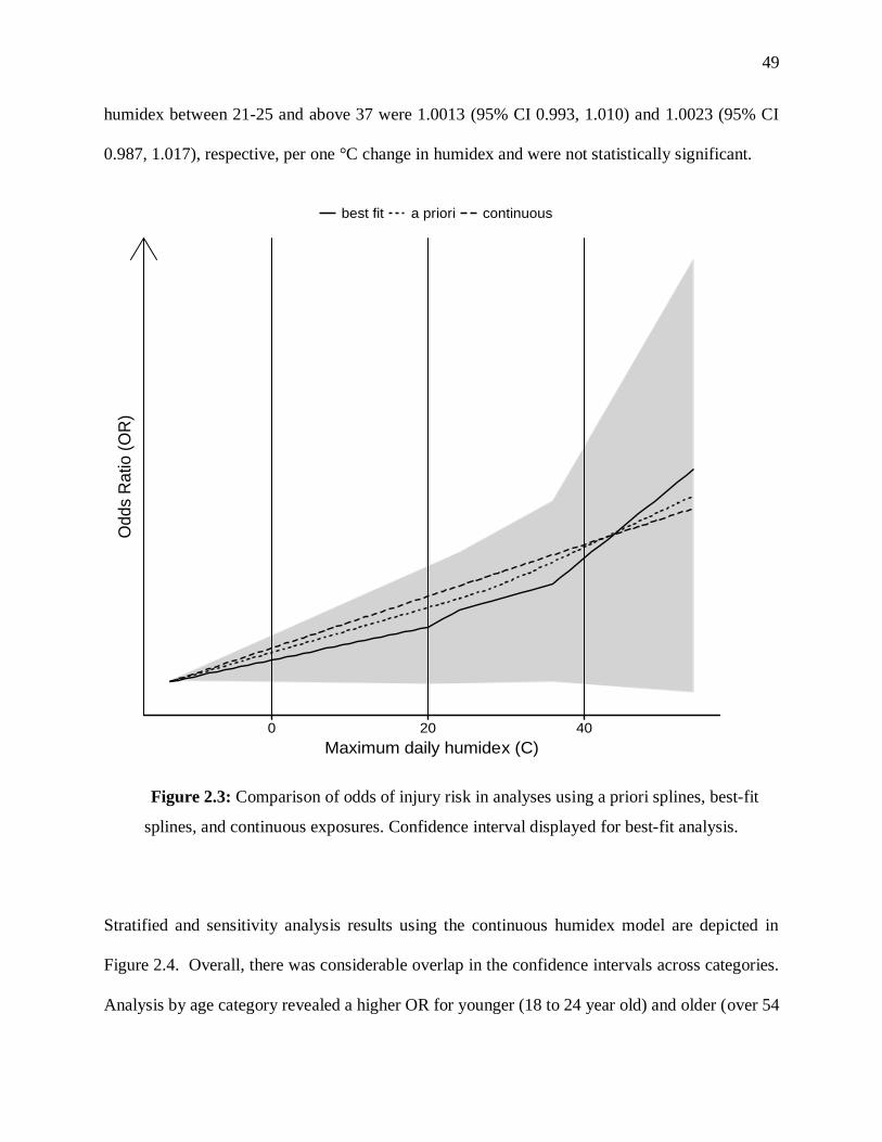
49
humidex between 21-25 and above 37 were 1.0013 (95% CI 0.993, 1.010) and 1.0023 (95% CI
0.987, 1.017), respective, per one °C change in humidex and were not statistically significant.
Figure 2.3: Comparison of odds of injury risk in analyses using a priori splines, best-fit
splines, and continuous exposures. Confidence interval displayed for best-fit analysis.
Stratified and sensitivity analysis results using the continuous humidex model are depicted in
Figure 2.4. Overall, there was considerable overlap in the confidence intervals across categories.
Analysis by age category revealed a higher OR for younger (18 to 24 year old) and older (over 54
0 20 40
Maximum daily humidex (C)
Odd
s R
atio (
OR
)
best fit a priori continuous
Change in Odds Ratio

50
years) worker claims. Lower extremity injury claims were also characterized by a higher OR as
were those associated with less worker experience. Lower ORs were observed for injuries
occurring later in the afternoon and for the large employer size (≥50 employees). The OR for
Eastern Washington was slightly lower than for Western Washington. Sensitivity analyses did not
result in substantially different relationships between humidex and traumatic injuries.
Figure 2.4: Stratified and sensitivity analyses.
●
●
●
●
●
●
●
●
●
●
●
●
●
●
●
●
●
●
●
●
●
●
●
●
●
●
Primary Case Definition
Age
Body Part
OIICS Event
Experience
Firm Size
Region
Time of Day
MET
Season
Geocoded Location
Days to 1st Provider
Geocoding Score
Time Loss
Outdoor Context
Previous Claims
0.989 1.000 1.010 1.020
Continuous exposure
55 or older45 to 5435 to 4425 to 3418 to 24
Multiple Body PartsTrunk
Lower ExtremityUpper Extremity
OtherBodily Reaction & Exertion
Falls
MoreLess
50 or more10 to less than 50
Less than 10
EasternWestern
1631 to 19311231 to 16300931 to 12300531 to 0930
>54 to 5
<4
May 1st through Sept 30th
Accident Address
Less than 2 days
0.8
Less than 7 days
80% or more
No previous injury claim
Odds Ratio
Pre
dic
tor
● Effect Modifier Main Effect Sensitivity Analysis
Effect Modification and Sensitivity Analyses

51
2.5 DISCUSSION
Our findings of an association of increasing occupational heat exposure with increasing risk of
traumatic injuries in WA outdoor construction contributes to the growing body of evidence
suggesting occupational heat exposure impacts the health and safety of workers beyond HRI. Our
results of potentially higher risk in younger and older workers, workers with lower extremity
injuries, workers with less job experience, smaller employers, workers working in Western
Washington, and time of injury before 12:30 pm provide opportunities for further study of the
nuances of this phenomenon in outdoor construction workers. A better understanding of these
nuances could lay the groundwork for construction injury prevention approaches that address the
role heat plays in the risk of an injury.
In the best-fit spline analysis, increasing humidex during warmer months of the year was
characterized by a nearly linear association with the risk of a traumatic injury. A similar trend in
effect estimates was seen in the a priori spline, continuous, and categorical exposure analyses.
This positive relationship is consistent with findings in the existing literature. In a study using a
similar modeling approach and population of interest, Xaing et al. reported an injury incidence rate
ratio (IRR) of 1.006 (95% CI: 1.002, 1.011) per degree °C increase in maximum daily temperature
between 14.2 and 37.7 °C for construction workers in Adelaide, Australia (Xiang et al., 2014).
This increase is on the same order of magnitude as the ORs reported in this study for the continuous
analyses using maximum daily humidex (OR 1.005 per degree °C; 95% CI: 1.003, 1.007) and
maximum daily temperature (1.007 per degree °C; 95% CI: 1.005, 1.009). Similarly, Adam-
Poupart et al. reported an IRR of 1.003 (95% CI: 1.000, 1.006) per degree °C increase in maximum
daily temperature in Quebec, Canada for construction workers, and McInnes et al. reported an OR
of 1.008 (95% CI: 1.001, 1.015) per degree °C increase maximum daily temperature in young

52
workers (<25 years of age) in Melbourne, Australia (McInnes et al., 2017). Using wet bulb globe
temperature (WBGT) as the metric for exposure, Garzon-Villalba et al.’s study of acute injuries in
Deep Water Horizon disaster cleanup workers reported a relative risk (RR) for acute injury of 1.13
(95% CI: 1.09, 1.17) above a maximum WBGT of 20 °C (Garzon-villalba et al., 2016). While
WBGT was not used in this study, the effect estimates are on a similar order of magnitude to those
found in this analysis.
In a study of agricultural workers in Eastern Washington using a categorical exposure approach,
Spector et al. report a peak OR of 1.15 for a maximum daily humidex between 30-33 °C, relative
to < 25 °C (Spector et al., 2016). This estimate is higher than the OR reported for a similar range
in exposure in this study (OR 1.09 for a maximum daily humidex between 30-34 °C, relative to
<17 °C). The higher OR in agriculture at lower humidex values may reflect differences in safety
culture, task-related hazards that are not characterizable with the available data, or payment
method, since piece-rate pay is more common in agricultural work and has been reported to be
associated with more symptoms of HRI and heat strain than hourly-payment methods (Spector et
al., 2015).
Consistent with McInnes et al (McInnes et al., 2017) and Adam-Poupart et al(Adam-Poupart et al.,
2015), who report linear relationships between increasing heat and increasing injury risk, we report
a near-linear relationship, with only slight non-linearity was observed in the best-fit spline analysis
and categorical exposure analysis. In the analysis using splines, we report greater per °C increases
in the OR at humidex between 21-25 °C and above 37 °C. The ranges in exposures associated with
these steeper slopes are noteworthy because they fall at humidex values considered to be
comfortable and at values above which periods of rest are recommended for workers who are

53
unacclimatized or are completing heavy physical work, respectively (Canadian Centre for
Occupational Health and Safety., 2011).
The near-linear trend in our results are, however, contrary to the findings of Spector et al (3), Xiang
et al (Xiang et al., 2014), and Morabito et al (Morabito et al., 2006), who report a reversed u-
shaped association between increasing heat and the risk of injury. While heat exposure metrics and
populations vary by study, injury risk has been reported to decline above a maximum daily
temperature of 37.7 °C (Xiang et al., 2014), maximum daily apparent temperature of 31.7 °C
(Morabito et al., 2006), and maximum daily humidex of 34 °C (Spector et al., 2016). It has been
hypothesized that the reversal of effects at the upper extremes of exposures are not the result of a
true reduction in risk at high temperatures, but rather reflect exposure misclassification related to
risk reduction practices used to prevent HRI, such as ending work shifts early on the hottest days.
Work organization and behavior is challenging to characterize using population data, such as
workers’ compensation claims, emergency department visits, or hospitalizations and may lead to
exposure misclassification. These factors, however, may be more accurately characterized in
workplace studies. Fogleman et al (Fogleman et al., 2005) used aluminum smelter company health
and safety records combined with hourly weather data to assess the relationship between heat and
injuries in aluminum smelter workers. In Fogleman et al’s study, where work hours and hourly
weather data were known, acute injury ORs were observed above exposures of 32°C.
Unlike in agriculture, less flexibility to modify work hours to avoid working during the hottest part
of the day may exist in construction. For example, noise and light ordinances may prohibit
construction activities outside of typical business hours. The pace of work may also be driven by
pressure to complete a task due to weather or material considerations, putting workers in a position
where they are unable to adequately self-pace or practice recommended work-rest cycles. In

54
addition, adjustment of work processes so that easier or less strenuous tasks can be completed
during periods of high heat stress, when workers often experience greater fatigue and productivity
is expected to wane, may be unattainable due to scheduling constraints and the nature of the tasks
needing to be completed. For example, framers may rush to finish load-bearing walls prior to the
delivery of trusses so as to avoid rescheduling the delivery for potentially a much later date.
Roofing workers may feel pressure to complete the water proofing of a building before the end of
the shift if the weather forecast indicates any chance of rain. Workers often need to work within
local regulations and accommodate the schedule of other trades (such as an elevator operator).
Large employers (50 or more employees) were characterized by a lower injury effect estimate in
stratified analyses than medium and smaller employers, although confidence intervals of effect
estimates for different categories of employer size overlapped. This finding is consistent with
findings by Xiang et al. where medium employers (20-199 employees) and large employers (≥200
employees) were characterized by lower injury effect estimates than small-sized employers (1-19
employees) (RR 1.004 and 1.000 compared with 1.007, respectively) (Xiang et al., 2014). Larger
employers in our study may have greater capacity to implement heat risk prevention strategies, are
required to have Safety Committees in Washington (WAC 296-800-130), and are more likely to
have the financial capacity to utilize health and safety technology and employ dedicated health
and safety specialists. There are also trends in employer size by other industry characteristics.
Smaller companies are more commonly involved residential work and larger companies in
commercial work (Holizki et al., 2015), and this may result in different occupation- or task-related
risk factors by employer size. Additional support for small businesses may be indicated to
effectively prevent heat-related traumatic injuries.

55
We did not find evidence suggestive of effect modification by MET level. Contributions to
occupational heat stress include environmental conditions, metabolic activity, and clothing. In this
study, metabolic activity was evaluated using MET estimates developed from the ATUS.
Metabolic activity is notoriously difficult to assess accurately, and values provided at an
occupational level cannot describe the variability in metabolic demands across tasks or even
individuals conducting similar work. Further work is needed to more accurately assess metabolic
activity in order to assess its contribution to occupational heat-related injuries.
Age is a known risk factor for heat-related health effects. We report that younger (18-24 years of
age) and older (over 54 years) claimants exhibited greater heat-related injury risk, although
confidence intervals of effect estimates for different categories of age overlapped. In a setting with
high metabolic demand and high ambient heat, older individuals may be more susceptible to the
effects of heat due to decreased skin blood flow (Holowatz & Kenney, 2010) and decreasing
cardiac capacity (Armstrong & Kenney, 1993), as well as have a higher prevalence of pre-existing
conditions. Young workers may be more likely to exert rather than pace themselves, may be more
likely to be assigned tasks with higher metabolic demands than their older counterparts, and have
been reported to display more negative attitudes towards safety and personal protective equipment
(Lombardi, Verma, Brennan, & Perry, 2009; Siu et al., 2003). In other similar research, higher risk
estimates have been reported for workers less than 25 years of age per °C increase in maximum
daily temperature in Australia (McInnes et al., 2017) and in Canada (Adam-Poupart et al., 2015).
None of these studies report higher risks for older workers, except for McInnes et al (2017), by
minimum daily temperature.
Less experience was also characterized by a higher injury effect estimate with less precision than
more experience in stratified analyses. We observed slightly less experience in the youngest age

56
category, with 73% of claimants age 18-24 categorized as having more experience compared with
80% for the full population. Claimants over 54 years of age were observed to have the most
experience (84%). Experience was defined as working in the previous quarter, according to ESD
data, or working for the employer for at least 90 days according the self-report data on the injury
claims form. This definition does not describe experience acquired over longer periods of time that
could influence a worker’s tasks, responsibilities, standing with an employer, or perceived job
security. However, this definition of experience is expected to reflect familiarity with processes
and tasks performed during the referent window as well as acclimatization to environmental
conditions present within a work environment. Research by Choudhry et al describes how actual
experience, in addition to training, is required to adequately prepare workers for the conditions
present on a job site, including the presence of heat and fast-paced work (Choudhry & Fang, 2008).
There were several possible factors that could contribute to a smaller effect in Eastern WA than
Western WA. The climate in Washington State is characterized by two distinct regions that are
separated by the Cascade Mountains: a relatively milder western region and an eastern region with
hotter, drier summers and colder winters. These different climates may affect patterns of
acclimatization (timing and threshold tolerance) and could trigger differences in heat-related
practices. These regions are also characterized by different economic and development profiles
with a larger, booming urban center in Western WA (Seattle-Tacoma) compared to Eastern WA.
The injury claims data were dominated by claims in the western region (80%). In addition to the
implications for precision of estimates, Western Washington data likely drove the knot selection
for the best-fit selection of spline model to a greater extent than the Eastern WA claims.
We observed higher ORs for injuries to the lower extremities than other parts of the body, although,
again, confidence intervals of ORs for body part categories overlapped. Of these injuries, the most

57
common precipitating event was falls (48%). In comparison, falls accounted for 34% of injuries
in the full dataset. This is consistent with existing literature attributing 50-60% of lower extremity
injuries to falls in non-military settings (Mackenzie & Fowler, 2008). Research investigating the
mechanisms suspected in the relationship between heat and traumatic injuries have focused on the
potential relationship between decrements to balance and cognitive performance, including
vigilance—mechanisms identified to increase the risk of falls—and conditions characterized by
heat stress. Changes in balance resulting from fatigue have been documented in controlled settings
related to extreme muscle fatigue (Parijat & Lockhart, 2008) and exercise in hot conditions
(Distefano et al., 2013), as well as in review articles of exercise-induced fatigue (Zemková &
Hamar, 2014). The association between fatigue and heat has been documented in similar controlled
settings (Ganio et al., 2011; Nielsen, Hyldig, Bidstrup, González-Alonso, & Christoffersen, 2001).
In some of this work, changes in cognitive performance have also been documented. Ganio et al
(Ganio et al., 2011) reported increased tension and anxiety as well as vigilance and memory errors
occurred under conditions of hyperthermia and dehydration; Mazlomi et al (Mazlomi et al., 2017)
reported higher levels of stress hormones, including cortisol, in foundry workers working in high
WBGT conditions; and Sharma et al (Sharma et al., 1983) reported a greater effect of heat on
psychological functions with humidity was also high. Other factors may also contribute to the
relationship between heat and traumatic injuries as well, such as changes in safe work practices
(Ramsey et al., 1983).
There are a number of potential explanations for why risk might decrease with later work-shift
hours that should be explored further. Tasks may differ by time of day. For example, tasks earlier
in the day may include more active movement to set up the site and move materials into place in
preparation for more stationary activities in later hours. Changes in task could affect metabolic
58
contribution to heat stress as well as traditional risk factors for injuries (e.g. trip hazards). Heat
exposure in the morning may also have been low enough so that workers did not recognize early
signs of HRI or heat strain, such as excessive sweating. These lower exposures would also likely
not have triggered HRI awareness or intervention tactics that may have been utilized later in the
day. Diurnal patterns have also been observed in vigilance and balance research, where
performance was worse in early morning tests. In field studies with agricultural workers in WA
State, Spector et al (Spector et al., 2018) observed significantly longer mean reaction time and a
greater number of lapses measured using a psychomotor vigilance test (PVT) as well as longer
mean total path length, a measure of postural sway, in pre-shift assessments (i.e. prior to a mean
shift start time of 06:00). Further research should investigate specific tasks and associated
metabolic heat production throughout the work-shift, construct task-related injury risk factor
profiles by time of day, and better characterize vigilance and postural sway within workers over
time and between workers.
2.6 STRENGTHS AND LIMITATIONS
A strength of this study is our novel approach to identify workers more likely to be working
outside. Separation of outdoor and indoor environments is particularly important for analyses of
heat in settings where the presence of air conditioning is inconsistent, such as construction sites in
the Pacific Northwest. In settings where air conditioning is available, the indoor environment may
be characterized by reasonably predictable cooler conditions. However, even when indoors,
construction work may occur prior to the installation or use of air conditioning or in areas of a
building not typically climate controlled, leading to unpredictable thermal conditions. Xiang et
al’s study (Xiang et al., 2014) included a high level separation of indoor and outdoor exposures by
grouping the construction sector with “agriculture, forestry, and fishing” and “electricity, gas, and

59
water” under the name “outdoor industries”. While this approach is an improvement over analyses
of all industries combined, it still includes some occupations with predominantly indoor work. Our
analysis takes advances this approach by excluding occupations within the construction industry
identified with less than 50% O*NET context outside. By restricting the inclusion criteria for
injury claims, we minimize non-differential exposure misclassification and reduce bias of results
towards the null. Further work is needed to better characterize the work environment by task, job
site, or other factors that could improve categorization of indoor and outdoor contexts.
The availability of both high-resolution meteorological data and injury location addresses enabled
spatial pairing of the outdoor conditions with the injury location at a higher resolution than has
been achievable in other studies of heat exposure and traumatic injuries in construction. This
approach to assigning environmental exposures also reduced the potential exposure
misclassification introduced by using one monitoring station per large geographic area
(representative weather stations) or aggregating across political boundaries (city-, county-, etc.).
These approaches do not account for variations in weather conditions and climate associated with
geographic features. The use of representative stations or mean exposures across political
boundaries also inherently minimizes the presence of extremes.
This study has several limitations. First, in nearly half of the claims, accident address was either
missing or not complete enough to be geocoded accurately. As a result there may have been
exposure misclassification from assigning the address of the first medical provider to the injury
location. Out sensitivity analysis suggests this missing data did not substantially alter the estimate
in the primary analysis.

60
Second, we were unable to take into account variability in clothing. Clothing is an important
consideration when assessing heat stress since it can act as an insulating barrier between the body
and the environment. WA workers’ compensation records do not contain systematic information
about a claimant’s clothing at the time of injury. We explored the use of personal protective
equipment (PPE) that would necessitate inclusion of a clothing adjustment factor by occupation
(SOC) using O*NET survey responses and expert opinion, but ultimately deemed clothing-related
PPE to be too difficult to quantify. Therefore, we did not stratify by clothing and assumed that
workers wore the same clothing on the day of injury and referent days.
The third limitation of this study was that we did not take into account solar radiation. In
occupational settings, the wet bulb globe temperature (WBGT) is often considered to be the gold
standard for measuring environmental heat and is central to recommendations by the United States
National Institute for Occupational Safety and Health (NIOSH), American Conference of
Governmental Industrial Hygienists (ACGIH), International Organization of Standardization
(ISO), US Armed Services, American College of Sports Medicine, and other
organizations(NIOSH, 2016). The WBGT assesses solar radiation through the black globe
temperature. Adjustment factors that take into account solar radiation have been used to estimate
WBGT from dry temperature and relative humidity alone (Bernard & Barrow, 2013). While the
validity of these calculations has been demonstrated (Bernard & Barrow, 2013) use of this
approach still hinges on knowledge of the presence or absence of solar radiation to inform use of
the appropriate equation: WBGT in the sun or WBGT in the shade. In large studies such as this
one, where a metric for clouds or solar radiation is not available in the meteorological data and
there exists substantial spatiotemporal variability in weather conditions, calculation of the WBGT
may increase non-differential misclassification of exposure. We therefore did not pursue

61
estimation of WBGT in this study. We were also unable to take into account differences in worker
microclimates influenced by point sources of heat, shade, or shift breaks. We assumed claimants
were working on the same job site and under the same conditions on referent days. Potential shifts
in work location, whether between multiple sites or even conditions within a site, may have
influenced a claimant’s exposure on injury and referent days.
Forth, we were unable to adjust for several potential time-varying confounders. At the individual
level, the task a worker performed may change as a result of an injury, where a claimant who
returned to work after an injury may have been placed on light duty, laterally shifted to a different
crew or worksite, or altered how he or she performed the task. Tasks may also change as a result
of the heat, where the claimant adjusted the timing of tasks to optimize productivity or comfort in
different weather conditions. The tasks also had the potential to change at the worksite or employer
level as a result of administrative controls or implementations aimed at the same outcomes.
Changes to worksite safety practices or awareness of HRI-prevention could also change as a result
of an injury or heat conditions. If such changes were implemented after injuries occurred early in
the referent window or due to high heat exposure, results would likely be biased toward the null.
2.7 CONCLUSIONS
Environmental heat exposure in outdoor construction workers in Washington State is positively
associated with traumatic injuries. For this population, we report a nearly linear association with
the risk of an injury at exposures lower than thresholds recommended in occupational health and
safety guidelines for heat stress controls based on HRI risk. Stratified analyses suggested higher
risk in younger (18-24 years) and older (over 54 years) workers, for lower extremity injuries,
workers with less job experience, smaller employers, workers working in Western Washington,

62
and time of injury before 12:30 pm, although there was there was overlap in confidence intervals
of effect estimates across categories. Further research is needed to better characterize metabolic
heat production within occupational groups, understand the mechanism of association between
heat exposure and traumatic injuries, and formally explore effect modification by key factors. The
findings in this study suggest that injury prevention efforts in construction should address heat-
related risk factors, particularly for high-risk workers. Additionally, this information could be
used to inform combined heat stress and injury prevention efforts in the highest risk construction
workers as well as expand broad occupational heat awareness campaigns to address outcomes
beyond heat-related illness.
Chapter 3. A COMPARISON OF OCCUPATIONAL HEAT
EXPOSURE MEASURED AT THREE SPATIAL
RESOLUTIONS IN COMMERCIAL ROOFING
WORKERS: IMPLICATIONS FOR HEAT HEALTH
RESEARCH AND PRACTICE.
3.1 ABSTRACT
Background: Exposure to heat is known to adversely affect health. In occupational settings, heat
exposure is traditionally quantified using area monitoring devices. Data from weather stations and
personal monitoring devices have also been used to assess heat-health relationships. The objective
of this analysis was to compare how regional-, area-, and personal-level measurement approaches
influence the quantification of environmental heat exposure in an occupational setting.
Methods: Full work-shift measurements of heat were collected in a sample of 22 commercial
roofing workers in the Greater Seattle area in a repeated-measures study during the summer and
63
fall of 2016. Measurements were made using county weather stations at the regional-level (RL),
3MTM QUESTempTM 36 Heat Stress Monitors at the area-level (AL), and hygrochron iButtons at
the personal-level (PL). Using the area monitor as the baseline, we described differences in air
temperature and wet bulb globe temperature (WBGT) measured at the personal and regional levels
as the difference from the area monitor, where a positive difference indicated a higher temperature
at the personal or regional level than measured at the area level. The Newey-West estimator was
used to adjust for temporal autocorrelation. Differences between worksites were quantified as the
standard deviation of the means from analyses stratified by site.
Results: We report a positive mean (95% confidence interval) difference between PL-AL
temperature of 4.4 (4.1, 4.7) °C and WBGT of 1.5 (1.3, 1.8)°C-WBGT, and a difference between
RL-AL temperature of 0.2 (-0.3, 0.6) °C-WBGT. The direction of the difference between regional
and area monitors varied by site with a standard deviation of site-specific mean differences of 1.04
°C. We observed variability in heat exposure in PL measurements that was not captured at the AL.
Conclusions: Personal measurement data were observed to be consistently higher than area data,
but the difference between regional and area monitors varied in direction by site. Differences in
heat measurements based on AL, RL, PL approaches may have implications for epidemiologic
study inferences and for workplace health and safety practice, where area-level measurements are
typically used in conjunction with occupational heat stress guidelines.
3.2 INTRODUCTION
Heat exposure can increase the risk of heat related illness (Bonauto et al., 2007; Kerr, Casa,
Marshall, & Comstock, 2013; NIOSH, 2016; Parsons, 2002; Michael N. Sawka et al., 2011;
Spector et al., 2014), which may be fatal if not treated promptly (Bouchama & Nochel, 2002;

64
Parsons, 2002; Michael N. Sawka et al., 2011). Heat stress in occupational settings may also reduce
performance and productivity (Lundgren et al., 2014; Mckinnon et al., n.d.; Sahu et al., 2013;
Zander, Botzen, Oppermann, Kjellstrom, & Garnett, 2015), increase the risk of a traumatic injury
(Adam-Poupart et al., 2015; Fogleman et al., 2005; Garzon-villalba et al., 2016; McInnes et al.,
2017; Morabito et al., 2006; Spector et al., 2016; Xiang et al., 2014), and adversely affect overall
quality of life through morbidity related to repeated exposure such as kidney damage. Recent
research suggests a relationship between heat exposure and acute kidney injury in US agricultural
workers (Moyce et al., 2017), and repeated intermittent dehydration related to heavy physical work
in hot conditions is hypothesized to contribute to chronic kidney disease of unknown origin
(CKDu), an emerging epidemic in Central America, Sri Lanka, and other areas of the world
(Orantes Navarro et al., 2015; Rajapakse, Shivanthan, & Selvarajah, 2016).
Thorough evaluation of the human thermal experience, or human heat balance, requires calculation
of energy produced through metabolic processes, energy transferred to and from the human body
from the surrounding environment, and the impact of factors influencing the efficiency of energy
transfers, such as clothing (McGregor & Vanos, 2017; Parsons, 2002; Michael N. Sawka et al.,
2011). Precise quantification of these factors is often problematic because of the inherent
challenges in estimating energy from numerous sources that may be in multiple forms (radiation,
convection, and conduction) and the perpetually changing nature of environmental conditions and
metabolic demands. Variability in heat removal efficiency between and within individuals based
on physical fitness, medical conditions, medications, age, and other factors (Parsons, 2002;
Michael N. Sawka et al., 2011) also complicates quantification efforts. Over the past century, many
rational, empirical, and direct indices have been developed to describe how humans perceive and
respond to the environmental conditions of their thermal environment (Brake & Bates, 2002;

65
Epstein & Moran, 2006; McGregor & Vanos, 2017; Parsons, 2002). The choice of indices depends
on the setting, availability of input parameters, exposures and outcomes of interest, regional
climate, and spatiotemporal scale. At a minimum, these metrics rely on climatic conditions. While
comparisons between these metrics have been conducted in a number of settings (Barnett et al.,
2010; Parsons, 2002), few comparisons have been reported where the same metric is measured at
different spatial and temporal scales (Basu & Samet, 2002; Bernhard et al., 2015; Kuras et al.,
2015).
3.2.1 High risk population: Roofing construction workers
In Washington State, the highest workers’ compensation injury claims rate for heat related illness
(HRI) during third quarter months (July, August, and September) was reported for the roofing
industry at 161.2 injury claims per 100,000 FTE for 1995-2005 (Bonauto et al., 2007). Roofing
work often involves exposure to the elements (National Center for O*NET Development, n.d.-c),
high metabolic demands (National Cancer Institute, 2016), and point-sources of heat, such as in
torch-applied roofing, where an open flame and hot air are used to apply localized heat to roofing
materials (OSHA, 2015).
Metabolic demands in roofing vary by task and often require activities such as walking, bending,
and lifting, moving, or cutting materials. Some tasks, such as operating a torch or hot air welder,
may involve less physical movement but still require energy from pushing, pulling, and holding
equipment (Parsons, 2002; Vezina et al., 2014). In addition to the standard work boots, long pants,
and t-shirt often worn by construction workers, built-up applications usually require long-sleeved
shirts to prevent burns from contact with hot tar; torch operators and precision workers may opt to
use heat-protective Kevlar sleeves. Roofing and other construction occupations may

66
disproportionately experience the anticipated climate-induced increases in the frequency, duration,
and severity of extreme temperatures due to the nature and location of their work in urban centers,
often on rooftops with no shading, where the effects of urban heat islands would be greatest.
3.2.2 Heat exposure assessment approaches at different spatial scales
In population level heat assessments, data collected through meteorological services (e.g. weather
stations) provide representative measurements for large geographic regions that can be used to
calculate direct indices, such as the wet bulb globe temperature (WBGT), humidex, or heat index.
These data are often available free of charge at up to a daily, if not sub-hourly, resolution for
current and historic conditions and are increasingly accessible with the growing use of smart
phones and robust networks of weather monitoring stations (King-TV, n.d.; The Weather
Company LLC, n.d.). Weather station data are appealing for retrospective assessments,
comparisons between different regions, and remote monitoring. In some settings, models have
been used to improve the spatial resolution of the data (Daly et al., 1997). However, even with
high-resolution meteorological data, point-sources of heat and microclimates are likely not
captured.
Increased precision of heat exposure measurements for an individual or group at a particular site
can be accomplished through the use of small, portable weather stations or area heat stress meters.
This approach can provide data at a higher temporal resolution and is particularly advantageous in
settings where a representative weather station is not expected to capture environmental
conditions, such as indoor settings (e.g. a factory) and underground (e.g. a mine). Heat stress
meters are used to provide heat stress assessments for populations with particularly high risks of
adverse heat-health outcomes, such as outdoor workers, and have been used as a basis for heat

67
stress recommendations for the military, workers, and athletes (Havenith & Fiala, 2016; NIOSH,
2016; Parsons, 2002). In occupational settings, a direct index, the wet bulb globe temperature
(WBGT), is usually captured by a WBGT meter positioned as close as possible to the work area,
or with several monitors “when the conditions vary substantially in the work area” (OSHA, 2017).
This approach is designed to assess the conditions of the job site rather than individual exposures
(American Conference of Governmental Industrial Hygienists, 2015) and can be inadequate in
assessing individual exposures when individuals move rapidly and repeatedly between different
environments (e.g. from hot attics to air-conditioned vehicles) or when resources (e.g. financial,
equipment, etc.) are sparse. WBGT monitors may cost between $500 to $4000, depending on the
model and data logging needs.
Monitoring of personal, or individual, heat exposure has been increasingly used in heat health
research (Bernhard et al., 2015; Kuras et al., 2017, 2015; Mitchell et al., 2017). Availability of
monitoring devices that are small, affordable, accurate, having data logging capabilities, and
capture parameters necessary to directly calculate heat indices facilitates mapping of an
individual’s thermal environment over time and space, when paired with GPS or location data and
time use surveys (Kuras et al., 2017). When coupled with personal-health, fitness, and physiology
tracking technology (e.g. heart rate monitors, activity monitors, etc.) there exists the potential for
individualized heat stress assessments and recommendations; a hugely prospect that is incredibly
advantageous for monitoring and intervention, as well as education, purposes. However, approach
is not without challenges, including identification of the best approach for affixing a device to an
individual so it captures the ambient environment rather than unintentional environments such as
within an individual’s jacket pocket and precise understanding of how temperature measured on
these devices compares with other monitoring strategies. Understanding how these measurements

68
relate to traditional monitoring approaches is critical for interpreting measurements in the context
of existing heat health guidelines and for research.
3.2.3 Study objective
The purpose of this study was to assess how different monitoring approaches (regional-, area-, and
personal-level) influence the quantification of environmental heat exposure in a sample of
commercial roofing workers in the Greater Seattle area. We hypothesized that in this population,
where task-specific point sources of heat are common and access to shade is rare, air temperature
measured at the personal-level would be higher and characterized by greater variability than
temperature measured at the area and regional level.
3.3 METHODS
Regional-, area-, and personal-level environmental heat exposures were measured in commercial
roofing workers in the Greater Seattle area during the summer and fall of 2016 as part of a larger
repeated measures study designed to assess the relationship between occupational heat stress, heat
strain, and traumatic injury risk.
3.3.1 Study population & recruitment
Commercial roofing workers were selected for the study population because roofing workers are
at high risk for adverse heat health effects (Bonauto et al., 2007), primarily work outdoors
performing tasks that require high metabolic demands (National Cancer Institute, 2016; National
Center for O*NET Development, n.d.-c), and often use task-specific point-sources of heat such as
hot-air torches (OSHA, 2015). Commercial, rather than residential, roofers were targeted for this

69
study to facilitate larger within-site sample sizes and to more easily allow for measurements over
multiple days per participant within the study’s geographic region.
Roofing companies in the Greater Seattle area were recruited during the winter and spring of 2016
to participate in the study using contacts through the University of Washington’s Department of
Construction Management. Enrolled companies provided a letter of consent to participate and
facilitated access to job sites with the site owners and general contractors, when applicable.
Participants were recruited from enrolled companies during small on-site safety meetings as well
as during an all-hands meeting—a large, quarterly safety meeting attended by all employees within
a company. Eligibility criteria are described in Chapter 4. Study researchers participated in safety
orientations on a site-by-site basis at the request of the general contractor or lead health and safety
specialist for each job site. All study procedures were approved by the University of Washington
Human Subjects Division, and participants provided written informed consent in advance of study
participation.
3.3.2 Data collection
All data collection was performed at the worksite for the full work-shift. Monitoring days were
selected based on two criteria: weather conditions and participant availability. We aimed to assess
each worker on one “hot” and one “cool” day. Forecasted weather conditions were monitored
closely through the National Weather Service. Days with forecasted maximum temperatures of
25°C or greater were anticipated to be “hot days,” and days with forecasted maximum temperatures
of 22°C or lower were anticipated to be “cool days”. At the end of each sampling day,
reclassification of the day as either hot or cool was performed based on area-level measurements
taken at the worksite. Days that did not meet the originally anticipated classifications were

70
reclassified such that the maximum temperature on cool days did not exceed 25°C and each
participant’s hot day was a minimum of 5°C hotter than his cool day. Each participant’s monitoring
days were scheduled a minimum of three days apart and, when possible, repeated measures were
performed at the same worksite.
3.3.3 Environmental measurements
Environmental measurements of heat were collected at three levels: personal, area, and regional
(Table 3.1). Personal-level (PL) measurements were collected using DS1923-F5 hygrochron
iButtons (Maxim Integrated; Son Jose, CA, U.S.) attached to the workers’ clothing using blue fobs
and carabiner-style attachments at approximately hip height. Workers were instructed not to cover
the devices with clothing or personal protective equipment (PPE). This location on the body was
selected based on research indicating that measurements taken from iButtons attached at foot,
waist, and neck height do not significantly differ on individuals exercising outdoors (Dumas,
Jagger, & K.W., 2016), considerations for potential task-related point-sources of heat directed at
the roofing surface and workers’ boots that could impact the vertical heat profile, and attainable
consistency in placement given differences in required personal protective equipment (PPE) such
as fall-protection harnesses by site. The devices measured and logged air temperature (Ta) and
relative humidity (RH) at two-minute intervals for the duration of the work-shift and remained on
the workers during breaks.
Area-level (AL) measurements were collected at the worksites using a 3MTM QUESTempTM 36
Heat Stress Monitor (3M; St Paul, MN, U.S.). The device was mounted on a tripod at
approximately one meter above the surface of the work site. Due to restricted access on many of
the worksites, researchers asked the study participants to position the area monitor in a location

71
Table 3.1: Monitoring devices by level and environmental variable.
Level Device(s) Monitoring
frequency Ta Tg Tnwb Tdew RH V
Personal Hygrochron iButtons 2 minutes ✓ ✓
Area 3M QuesTemp 36 3 minutes ✓ ✓ ✓ ✓
Regional NOAA weather
station 1 minute ✓ ✓ ✓
Air temperature (Ta), black globe temperature (Tg), natural wet bulb temperature (Tnwd), dew point temperature
(Tdp), relative humidity (RH), and pressure (V)
that was as close as possible to their work area, was representative of work conditions (i.e. in the
sun if the workers were in the sun), and would not be in the way of work-related tasks. Participants
were asked to re-position the monitoring device in the event the work moved to a different area
during the shift. The QUESTemp collected dry temperature (Ta), black-globe temperature (Tg),
natural wet bulb temperature (Tnwb), and relative humidity (RH) at three-minute intervals and
remained on the worksite during breaks. Prior to data collection, the QUESTemp was factory
calibrated and tested against the iButtons in a controlled, indoor setting to verify consistency of
measurements across monitoring devices.
The regional-level (RL) measurements were sourced from National Oceanic and Atmospheric
Administration (NOAA) Automated Surface Observing System (ASOS) for weather stations at
county airports in the two counties in which monitoring occurred: Seattle Tacoma International
Airport and Everett Snohomish County Airport (National Climate Data Center (NCDC), n.d.). This
data source was selected for consistency with other similar assessments of personal heat exposure
(Basu & Samet, 2002; Bernhard et al., 2015; Kuras et al., 2015) as well as epidemiologic studies
assessing the heat and heat related health effects at a city or regional level (Bernard & Barrow,
2013; Lemke & Kjellstrom, 2012; Lin, Wang, Chiang, Peng, & Yang, 2013; Nguyen, Schwartz,
72
& Dockery, 2014; Rhea et al., 2012; White-Newsome et al., 2012) and is representative of data
that may be available to the population of interest from local weather services, phone weather
applications, etc. Weather station observation data were available at one minute intervals (National
Oceanic and Atmospheric Administration, Department of Defense States, Federal Aviation
Administration, & United States Navy, 1998) for dry temperature (Ta) and dew point temperature
(Tdp).
3.3.4 Metabolic heat production
Metabolic heat production resulting from physical activity was estimated using hip-mounted
ActiGraph GT3Xs and accompanying ActiLife software (ActiGraph; Pensacola, FL, U.S.). These
tri-axial accelerometers measured changes in movement on three planes that were then converted
to estimates of daily (kcal/day) and hourly (kcal/hour) mean energy expenditure (EE) using
proprietary filters and the Freedson VM3 equation (Sasaki, John, & Freedson, 2011). Since the
area- and personal-level exposure monitors measured heat at a higher temporal resolution (e.g.
every 6 min), hourly EE values were assigned to all time intervals within a given hour; for example,
the EE for 13:00 to 14:00 was assigned to time intervals from 13:00, 13:06, 13:12, 13:18, … to
13:54. This allowed for calculation of rolling hourly averages over the entire workshift. Hourly
metabolic activity is relevant to occupational recommendations that are often based on hourly
interventions such as work-rest cycles (American Conference of Governmental Industrial
Hygienists, 2015; NIOSH, 2016).
In order to compare the values produced from the ActiGraphs with NIOSH and ACGIH
occupational recommendations for heat exposure, the participant’s daily resting (or basal) energy

73
expenditure (REE) was calculated using the Mifflin-St. Jeor Equation (Eq Error! Reference
source not found.) for males.
REE = 9.99weight + 6.25height – 5age +5, 3.1
where REE is in kcal/day, weight is in kg, height is in cm, and age is in years (Mifflin et al., 1990).
Daily REEs were converted to kcal/hour and added to the hourly estimates of EE, which were then
converted to Watts by multiplying by 1.163.
3.3.5 Clothing and worksite characteristics
Additional data were collected by researcher observation and photographs, including worker
clothing and worksite characteristics, such as the height of the building and proximity to water,
other buildings, and trees. Workers reported roofing processes and task-related point-sources of
heat during the shift directly to research staff. Characteristics of roofing processes used in the
previous week were assessed using an adapted computer-assisted survey instrument administered
electronically using hand-held tablets (Spector et al., 2015). This information was used to
descriptively inform the understanding of differences across worksites.
3.3.6 Exposure metrics
The primary metric used for comparison of heat exposure in this analysis was temperature (Ta),
which was directly available at all three spatial resolutions. Two direct indices of heat exposure
were calculated for use in secondary analyses: wet bulb globe temperature (WBGT) and Humidex.
All methods and results pertaining to Humidex are reported in Appendix X. WBGT was reported
by the area-level monitoring device (QUESTemp). Regional- and personal-level WBGT was
calculated from temperature and relative humidity using the following equations:

74
RH =100 e
17.625*Tdp( )/(243.04+T
dp)æ
èöø
/ e17.625*T
a( )/(243.04+Ta
)( )é
ëê
ù
ûú
3.2
P
v= RH /100( ) 0.61067e
17.27*Ta( )/(T
a+237.2)( ) , 3.3
T
pwb= 0.0376 + 5.79P
v+ 0.388 - 0.0465P
v( )Ta 3.4
T
nwb= 0.0376 + 5.79P
v+ 0.388 - 0.0465P
v( )Ta+ 1.0, 3.5
T
g= T
a+ DT
g-a, 3.6
WBGT
outdoors= 0.7 T
nwb( ) + 0.2 Tg( ) + 0.1 T
a( ) , 3.7
where Tdp is the dew point temperature (°C), RH is relative humidity (%), Ta is dry bulb
temperature (°C), Pv is vapor pressure (kPa), Tnwb is the natural wet bulb temperature (°C), Tpwb is
the psychometric wet bulb (°C), Tg is the globe temperature (°C), ΔTg-a is the difference in globe
temperature from the dry bulb temperature measured using the QuesTemp at the area-level (°C),
and WBGToutdoors (°C-WBGT) (Bernard & Barrow, 2013). This approach to calculating WBGT
from meteorological data is accurate within a 95% confidence interval of 2 °C-WBGT. Liljegren
et al. 2008 (Liljegren, Carhart, Lawday, Tschopp, & Sharp, 2008) present an approach with greater
precision (within 95% CI of 1 °C-WBGT), however it requires additional parameters not available
in the personal monitoring data .
3.3.7 Occupational thresholds
Two occupationally relevant exposure thresholds were calculated using equations 8 and 9 below:
1) the U.S. National Institute for Occupational Safety and Health (NIOSH) Recommended
Exposure Limit (REL) for acclimatized workers; and 2) the Recommended Action Limit (RAL)
for unacclimatized workers (NIOSH, 2016). These equations are identical to those used by the
75
American Conference of Governmental Industrial Hygienists (ACGIH) Heat Stress/Strain
Threshold Limit Value (TLV) and Action Limit (AL) (ACGIH, 2008).
REL = 56.7– 11.5log
10M , 3.8
RAL = 59.9– 14.1log
10M , 3.9
where the REL and RAL are in °C-WBGT and M is the metabolic rate in watts (joules/second)
(Garzon-Villalba, 2016; NIOSH, 2016) calculated as the mean metabolic rate for the study
population.
3.3.8 Statistical Analysis
Descriptive statistics were used to summarize measurements, including Ta, RH (since it is used to
calculate personal and regional WBGT), and WBGT for the full study and by exposure
classification (“hot” and “cool” days). The differences in temperature measurements across the
three levels were calculated using the area level measurements as the reference. To account for
different measurement frequencies of each monitoring device, six minute intervals were calculated
for data at all three levels for calculation of the differences. Means were calculated from the
difference at each six-minute interval between two datasets (each personal or regional dataset and
the corresponding area data) before averaging across time. A positive difference indicated the
measurement of heat at a given level (PL or RL) was greater than at the AL.
In the primary analysis, differences in Ta across monitoring levels were described using descriptive
statistics and box and whisker plots for different shift activity categories (full work shift, time
working only, and breaks only) and grouped into eight exposure categories (<10, 10-15, 15-20,
20-25, 25-30, 30-35, 35-40, and 40-45°C) by the AL as well as by the PL or RL. Paired t-tests
were conducted to test for statistically significant differences across monitoring levels. The

76
Newey-West estimator was used to adjust for temporal autocorrelation (Zeileis, Lumley, Berger,
& Graham, 2017). Differences were also stratified by exposure classification (hot and cool days),
worksite ID, metabolic activity (for PL-AL only), date, and time of day. The impact of the site on
the difference between monitoring levels was described as the mean and standard deviation of site-
specific differences for both the PL-AL ad RL-AL analyses.
Secondary analyses were conducted using WBGT, measured at the AL and calculated for the PL
and RL, as the metric of heat exposure using a similar approach to the primary analysis.
Additionally, the number of days and total number of monitored shifts during which the WBGT
met or exceeded the NIOSH heat stress/heat strain REL and RAL were compared across all three
monitoring levels. Since occupational thresholds are designed for one hour time weighted average
(TWA) exposures, the rolling hourly-mean WBGT was calculated for all three levels such that the
value at a given time represents the previous hour (e.g. WBGT at 13:00 is the mean of 12:01-
13:00). The earliest time at which the WBGT exceeded a threshold was compared for days where
multiple levels exceeded a threshold.
All analyses were conducted using R, and figures were produced using the ggplot2 package. (R
Development Core Team, 2011). The Newey-West estimator was implemented using the sandwich
package (Zeileis et al., 2017), and rolling means were calculated using the zoo package in R
(Zeileis, Grothendieck, Ryan, Urlich, & Andrews, 2018).
3.4 RESULTS
3.4.1 Sampling, work, and worker characteristics
Twenty-two commercial roofing workers from two companies in the Greater Seattle area
participated in the study during the summer and fall of 2016 (Table 3.2). Of these participants,

77
twenty participated on cool days, twenty-one participated on hot days, and one completed an
additional hot day, resulting in a total of 42 full-shifts measured throughout the study. Due to
monitoring device error, two cool days and one hot day were removed from the analysis for a total
of 39 shifts. These 39 shifts were collected across 13 days (six hot and seven cool) at seven
worksites with a mean of three workers monitored per day.
All participants were male with a mean (standard deviation) age of 43 (12) (Table 3.2). Shifts
typically started around 6:45 and ended around 15:04. All participants took a lunch break, with a
mean duration of 38 minutes, and 34 of the 39 shifts included a morning break, but no shift
included an afternoon break. The median number of days between repeated measures was fourteen,
and the repeated measures were collected on the same worksite in sixteen of the seventeen workers
who completed both hot and cool day measurements.
Worksites varied in physical characteristics as well as roofing processes. Sites ranged in height
from one to fourteen stories tall and were located across downtown urban, residential, and
industrial settings. Access to and utilization of shade varied by site. None of the sites had consistent
access to shade during work activities. On three sites, workers came off the roof during lunch break
and sat under trees or other more formal structures attached to the building. On two sites, the
workers remained on the roof during lunch breaks, but had shade access either from covered
sections of the building itself or man-made structures using portable tents. The remaining two sites
had inconsistent access and use of available shade.
The most commonly used roofing processes in this study were torch applied (“torchdown”)
roofing, followed by single-ply applications involving hot work. Of the seven sites and 39 shifts
monitored, only one site, where three participants completed both days of participation (totaling

78
six shifts), used a heat-free single-ply membrane application. One site, where only one cool-day
shift was monitored, used a built-up roofing application involving hot tar. However even on sites
Table 3.2: Sampling characteristics and worker demographics
Statistic
Full study
(hot and
cool days) Hot days Cool days
Companies n 2 2 2
Sites n 7 6 7
Days n 13 6 7
Participants n 22 21 18
Participants per day mean (sd) 3 (1) 3.5 (0.5) 2.6 (1.3)
Participants with repeated measures n 17 - -
Repeated measures at same worksite nyes/n 16/17 - -
Time between repeated measures
(days) median (min, max) 14 (9, 83) - -
Work characteristics by shifts
monitored number of shifts 39 21 18
Start time (H:M) mean (sd) 6:45 (00:23) 6:40 (00:22) 6:51 (00:23)
End time (H:M) mean (sd) 15:04 (00:53) 14:48 (1:06) 15:29 (00:37)
AM break (yes no) nyes/n 34/39 19/21 16/18
AM break duration (minutes) mean (sd) 20 (1) 22 (9) 20 (7)
Lunch break duration (minutes) mean (sd) 38 (10) 35 (9) 40 (11)
Used hot process during shift nyes/n 18/39 11/21 7/18
Participant demographics
Age (years) mean (sd) 43 (12)
Gender % male 100 Metabolic load for all shifts
combined
Rest (≤116 W) % of time 1.4% 1.1% 1.6%
Light (117-233 W) % of time 38.8% 46.3% 31.7%
Moderate (234-349 W) % of time 45.9% 48.5% 43.4%
Heavy (350-465 W) % of time 8.7% 0.0% 16.9%
Very Heavy (≥466 W) % of time 5.2% 4.1% 6.4%

79
with similar roofing materials and methods, monitoring days captured different stages within these
processes, such as tearing off old roofing material, laying down new roofing material, and general
site safety, set up, or material unloading. Tasks also ranged between and within workers even on
the same worksite. Participants reported tasks involving hot tools or materials on eleven of the
twenty-one hot day shifts, and seven of the eighteen cool day shifts, with more of these activities
being completed in late morning or afternoon (Table 3.2).
3.4.2 Exposure characteristics
The mean (interquartile range) temperature (Ta) of all six-minute interval, area level data was 20.1
°C (16.1 °C, 24.1 °C) for the full study (Table 3.3). Hot and cool days were characterized by a
mean (IQR) Ta of 24.3 °C (21.5 °C, 26.8 °C) and 16.7 °C (14.0 °C, 19.5 °C), respectively. The
mean (minimum, maximum) within person difference in maximum shift AL Ta between hot and
cool sampling days was 7.5 °C (4.3 °C, 12.4 °C). Exposure characteristics for humidity and WBGT
are available in Table 3.3.
3.4.3 Metabolic heat production
The mean (standard deviation) energy expenditure for the study population was moderate at 270.4
W (105.4 W), with a slightly higher mean on cool days (278.8 W [106.0 W]) than on hot days
(262.7 W [104.3 W]). Energy expenditure peaked between 8:00 – 9:00 on cool days and 7:00 –
8:00 on hot days and then steadily decreased with increasing hours throughout the shift as well as
increasing ambient temperature. For the study as a whole, participants spent 1.4%, 38.8%, 45.9%,
8.7%, and 5.2% of their time in rest (≤116 W), light (117-233 W), moderate, (234-349 W) heavy
(350-465 W), and very heavy (≥466 W) metabolic loads, respectively (NIOSH, 2016) (Table 3.2).

80
On cool days, slightly more time was categorized as heavy or very heavy, with reduced time in
light and moderate categories, while on hot days the opposite was observed.
Table 3.3: Exposure characteristics by monitoring level and metric for the full study, hot
days only, and cool days only. Statistics include the number of (six-minute average)
measurements (n), mean, and interquartile range (IQR).
Day Level n Air Temperature (°C) WBGT (°C-WBGT) Relative Humidity (%)
All
Personal 3241 25.6 (22.1, 29.1) 22.9 (20.6, 25.6) 51.9 (42.1, 63.6)
Area 1101 20.1 (16.1, 24.1) 20.4 (16.5, 24.5) 50.1 (33.0, 66.7)
Regional 1113 20.2 (15.6, 24.3) 18.9 (15.9, 22.4) 61.4 (45.9, 75.6)
Hot
Personal 1682 28.2 (25.1, 31.3) 24.7 (23.1, 26.7) 47.4 (36.1, 57.2)
Area 493 24.3 (21.5, 26.8) 23.9 (22.8, 25.9) 37.4 (27.7, 40.7)
Regional 496 25.1 (22.1, 28.4) 22.2 (20.7, 23.9) 48.0 (36.2, 57.6)
Cool
Personal 1559 22.7 (19.8, 25.9) 21.0 (18.8, 23.5) 60.6 (48.2, 70.4)
Area 608 16.7 (14.0, 19.5) 17.6 (14.7, 20.8) 60.4 (43.6, 75.3)
Regional 617 16.3 (13.3, 19.4) 16.2 (13.7, 18.4) 72.2 (62.2, 83.6)
The greater n in the personal data compared with the area and regional data is attributable to monitoring of
multiple subjects per worksite (area monitor).
3.4.4 Primary analysis
We observed the hypothesized positive difference between the PL-AL, indicating higher
temperature measured in the personal monitors. In this study, the mean (95% confidence interval)
difference in the PL-AL Ta was 4.4 (4.1, 4.7) °C for the full shift. The mean difference during
work activities only was slightly higher, while during breaks it was observed to be lower (Table
3.4). Without accounting for differences between sites, the mean (95% confidence interval) of the
RL-AL difference in Ta was 0.2 (-0.3, 0.6) °C. The difference during activities was identical,
however breaks were characterized to be slightly higher.

81
When stratified by the seven worksites monitored in this study, the mean RL-AL differences
calculated using the Newey-West estimator differed by a standard deviation of 1.04 (Table 3.5),
with negative relationships observed in two sites, strongly positive relationships observed in three
sites, and weaker positive relationships observed in the final two sites. Variability was observed
in the site-specific comparison of PL-AL differences as well (SD 0.88), although all differed in
the same direction.
Table 3.4: Differences in exposure by level. Statistics include number of measurements (n),
mean, standard error (se), and 95% confidence intervals (95% CI) using Newey-West estimator.
Temperature (°C) WBGT (°C-WBGT)
n Mean 95% CI n Mean 95% CI
Δ Personal - Area
Full Shift 3241 4.4 (4.1, 4.7) 3241 1.5 (1.3, 1.8)
Work Activities 2870 4.6 (4.3, 5.0) 2870 1.7 (1.4, 2.0)
Break Activities 344 3.0 (2.2, 3.8) 344 0.5 (-0.3, 1.2)
Δ Regional - Area
Full Shift 1113 0.2 (-0.3, 0.6) 1113 -1.6 (-2.0, -1.1)
Work Activities 1003 0.2 (-0.3, 0.6) 1003 -1.5 (-2.0, -1.0)
Break Activities 110 0.4 (-0.3, 1.0) 110 -1.9 (-2.4, -1.3)
When assessed by temperature category, the pattern in the magnitude of the difference between
PL-AL during work activities changed based on the level used to construct the categories (Table
3.6). By AL, the mean difference slightly decreased from 5.6 at Ta <10 °C to 3.9 at Ta between 30-
34 °C (the highest observed AL Ta range), but by PL, the difference increased from 0.9 at Ta <10
°C to 11.1 at Ta between 40-44 °C. When stratified by hot and cool monitoring days, the PL- AL
difference within each PL Ta category was greater on cool days than hot days (Figure 3.1). This
was also the case when compared across shift hours, with a noticeably greater difference during
mid-day when participants were on lunch break and the hot-day differences were minimized
(Figure 3.3a). In the RL-AL differences, the change across categories was substantially smaller

82
than in the PL-AL comparison. By RL Ta category, the trend was similar to in the PL-AL analysis
by PL Ta category, however the difference started negative in the <10 °C category and increased
to a positive value in the 30-34 °C category. By AL Ta category, the mean difference dipped in the
middle categories from a positive to a negative difference. When stratified by hot and cool days or
by time, the RL-AL differences showed little to no difference by hot versus cool monitoring day
(Figure 3.2) and no obvious change in the pattern during break periods (Figure 3.3b). However,
hot and cool day differences did diverge in the later hours of the shift, with the hot days
characterized by an increasingly positive difference and the cool days hovering slightly below zero
(Figure 3.3b).
Table 3.5: Differences in exposure levels by site. The mean and standard deviation of
the site-specific mean differences between levels is presented along with the site-specific
mean, standard error, and 95% confidence intervals of the difference between levels
calculated using the Newey-West estimator.
Temperature WBGT Mean SD Mean SD
Δ Personal - Area 4.60 0.88 1.80 0.88
Δ Regional - Area 0.05 1.04 -1.59 0.58
Site n Mean SE 95% CI Mean SE 95% CI
Δ P
erso
nal
- A
rea A 417 3.57 0.33 2.91 4.22 0.98 0.46 0.07 1.90
B 524 3.57 0.42 2.73 4.41 1.35 0.40 0.54 2.16
C 413 4.76 0.43 3.89 5.62 1.84 0.21 1.42 2.27
D 687 4.15 0.28 3.60 4.71 1.11 0.20 0.71 1.50
E 482 5.56 0.33 4.91 6.21 2.09 0.25 1.59 2.59
F 638 4.81 0.35 4.11 5.50 1.66 0.27 1.12 2.20
G 80 5.76 0.74 4.28 7.25 3.59 0.44 2.71 4.47
Δ R
egio
nal
- A
rea A 168 -1.35 0.31 -1.98 -0.72 -2.57 0.96 -4.49 -0.66
B 154 0.75 0.89 -1.03 2.52 -1.34 1.01 -3.36 0.67
C 209 0.26 0.81 -1.35 1.87 -0.68 0.50 -1.68 -1.22
D 175 0.61 0.18 0.25 0.98 -1.76 0.27 -2.29 -1.22
E 162 0.77 0.38 0.01 1.53 -1.86 0.83 -3.52 -0.20
F 165 0.86 0.38 0.11 1.61 -1.38 0.24 -1.86 -0.90
G 80 -1.53 0.43 -2.40 -0.66 -1.56 0.60 -2.76 -0.35

83
3.4.5 Secondary analyses
The mean (95% confidence interval) of the PL-AL difference in WBGT was 1.5 (1.3, 1.8) °C-
WBGT, 1.7 (1.4, 2.0) °C-WBGT, and 0.5 (-0.3, 1.2) °C-WBGT for the full shift, during work
activities only, and during breaks, respectively (Table 3.4). The mean (95% confidence interval)
of the RL-AL difference in WBGT was -1.6 ( -2.0, -1.1) °C-WBGT, -1.5 (-2.0, -1.0), and -1.9 (CI
-2.4, -1.3) °C-WBGT for the full shift, during work activities only, and during breaks, respectively
(Table 3.4). All differences observed by site in the RL-AL analysis were negative with a standard
deviation of site means of 0.58 (Table 3.5).
Table 3.6: Difference in exposure by temperature (°C) category during work activities
only. Statistics include the number of (six-minute average) measurements (n), mean,
standard error (se), and 95% confidence intervals (95% CI).
By Area Ta (°C) By Personal/Regional Ta (°C)
n Mean SE 95% CI n Mean SE 95% CI
Δ P
erso
nal
- A
rea T
a
less than 10 59 5.6 0.99 3.7 7.6 3 0.9 0.05 0.8 1.0
10 to 14 213 4.9 0.28 4.4 3.2 67 2.6 0.28 2.1 3.2
15 to 19 991 5.0 0.24 4.6 5.5 345 3.3 0.29 2.7 3.9
20 to 24 884 4.5 0.20 4.1 4.9 891 4.1 0.21 3.7 4.6
25 to 29 656 4.2 0.24 3.7 4.6 960 4.9 0.29 4.3 5.4
30 to 34 47 3.9 0.44 3.0 4.7 491 5.6 0.32 5.0 6.3
35 to 39 - - - - - 104 7.4 0.63 6.2 14.9
40 to 44 - - - - - 9 11.1 1.88 7.4 14.9
Δ R
egio
nal
-
Area T
a
less than 10 30 2.3 1.54 -0.8 5.4 28 -0.5 0.63 -1.8 0.7
10 to 14 146 -0.4 0.35 -1.1 0.3 204 -0.6 0.50 -1.6 0.4
15 to 19 336 -0.1 0.33 -0.8 0.5 274 -0.5 0.28 -1.1 0.0
20 to 24 275 -0.1 0.25 -0.6 0.4 275 0.4 0.43 -0.4 1.3
25 to 29 189 1.2 0.31 0.6 1.8 173 1.3 0.24 0.8 1.8
30 to 34 15 0.2 0.26 -0.3 0.8 49 1.8 0.57 0.7 3.0
Using the mean energy expenditure of the study population, 270.4 W, the NIOSH REL was
determined to be 28.7 °C and the RAL 25.6 °C-WBGT. The REL was never exceeded in the rolling

84
hourly-mean RL monitoring data, however it was exceeded on two days in the rolling hourly-mean
AL data and on three hot days in the rolling hourly-mean PL data. The RAL was exceeded on one
day in the RL data, five days in the AL data, and all six hot days as well as three cool days in the
PL data. Comparing the number of shifts measured (at the PL level) or represented (at the AL and
RL levels), no shifts, eight shifts, and six shifts exceeded the REL using RL data, AL data, and PL
data, respectively. Four shifts, eighteen shifts, and twenty-seven shifts exceeded the RAL using
RL data, AL data, and PL data, respectively. Using the day in which all three levels exceeded the
RAL for comparison (Figure 3.4), the earliest time at which the rolling mean WBGT for the
previous hour exceeded the RAL in the RL, AL, and PL data was at 11:48, 10:06, and 8:54,
respectively. For the REL, this occurred at 12:42 and 10:36 in the AL and PL data, respectively.
We did not observe a consistent difference in the time of first exceedance by task or process in the
PL.

85
Figure 3.1: Difference in PL-AL Ta by exposure categories stratified by hot (red bars) and
cool (blue bars) days. (A) Work periods by AL Ta. (B) Work periods by PL Ta. (C) Break periods
by AL Ta. (D) Break periods by PL Ta.

86
Figure 3.2: Difference in RL-AL Ta by exposure categories stratified by hot (red bars) and
cool (blue bars) days. (A) Work periods by AL Ta. (B) Work periods by RL Ta. (C) Break periods
by AL Ta. (D) Break periods by RL Ta.

87
A
B
Figure 3.3: Difference in PL-AL and RL-AL Ta by time stratified by hot (red bars) and cool
(blue bars) days. (Top) PL-AL by time of day. (Bottom) RL-AL by time of day. Median lunch
break start and end times were 11:55 and 12:30.

Figure 3.4: Exposure on the two days with area level exceedance of NIOSH REL for 270.4
W metabolic activity
3.5 DISCUSSION
This is the first published study that we are aware of to compare heat exposure metrics measured
at three distinct spatial resolutions—regional-, area-, and personal- (or individual-) levels—in an
occupational setting with exposure to outdoor weather conditions, work-related metabolic
89
demands, and process-dependent point-sources of heat. We report a positive difference in air
temperature and WBGT at the PL compared to the AL. The difference between the RL and AL
temperature varied by site, with some sites exhibiting negative differences and others positive. All
of the site-specific differences in the RL-AL WBGT were negative, indicating the area WBGT
was on average higher across all sites monitored in this study. These findings inform the
interpretation and application of different monitoring strategies and sources of exposure data to
research and practice.
Our overall finding—a mean difference in temperature of 4.4 °C from personal to area (PL-AL)
and relatively similar regional and area temperatures (Table 3.4)—demonstrates that area and
regional measurements have the potential to underestimate the magnitude of temperatures
experienced at the personal level. The variability observed in the mean difference between the RL-
AL observations by site suggests the presence of microclimates within the geographic area
represented by meteorological weather data. These differences may be the result of variability in
environmental conditions, work-related sources of heat, or, most likely, a combination of the two,
including the presence of dark impermeable surfaces, proximity to building ventilation, heat-
producing machinery, etc. (Oke, 1982; Rosenzweig, Solecki, & Slosberg, 2006; Taha, 1997).
These results are consistent with results reported by Kuras et al (2015), where neighborhood Ta
measurements, collected use iButtons placed in trees in the South End in Boston, MA were slightly
higher than weather station data from Logan International Airport during a summer heat wave
(Kuras et al., 2015), demonstrating a site-specific difference in temperature.
The magnitude and direction of the PL-AL observations suggest that area monitors inadequately
capture differences within and between workers on a worksite, such as those resulting from point-
sources of heat emitted closer to the workers than the area monitoring device, movement between

90
sun and shade, and human-emitted long wave radiation or heat removed from the body through
convective energy transfer (McGregor & Vanos, 2017; Parsons, 2002). While not directly
comparable, this strong positive difference is inconsistent with results reported by Bernhard et al
(2015) for occupational heat exposure in groundskeepers in Alabama, where temperature
measured at the personal level was slightly lower than weather station data. Differences between
the occupational settings of groundskeepers and roofers, including less impermeable surfaces and
the absence of point-sources of heat in groundskeeping work, may explain these contrary findings.
Two other studies comparing PL Tas with weather station data also report lower PL Tas than RL
Tas, but monitor different populations and include time indoors, often with air conditioning, in the
analysis (Basu & Samet, 2002; Kuras et al., 2015).
Utilization of breaks to reduce occupational heat stress in high heat environments and/or from
tasks requiring high metabolic demand is strongly recommended in occupational settings (Brake
& Bates, 2002; Hsie, Hsiao, Cheng, & Chen, 2009; Mckinnon et al., n.d.; NIOSH, 2016; OSHA,
2011). We observed a smaller mean difference in Ta during breaks than during work in the PL-AL
comparison (Table 3.4). This change in the difference between the PL-AL suggests that workers
were seeking cooler, shaded environments and reducing metabolic activity during these periods of
intentional rest, a behavioral practice that was observed by study researchers, however none of the
participants were observed to take breaks indoors or in climate controlled settings (such as a
personal vehicle with air conditioning). This difference is particularly dramatic when higher
temperatures were recorded (Figure 3.1, 3.3a). In contrast, RL and AL measurements were not
significantly influenced by personal break behavior, and RL-AL differences were similar during
breaks and work (Figure 3.2, 3.3b). In secondary analyses, the difference in WBGT levels between
breaks and work followed similar trends to the analysis of Ta.
91
We observed a greater positive mean difference in PL-AL Ta at higher PL Ta than lower PL Ta
(Figure 3.1b). In contrast, the PL-AL difference remained relatively consistent during work
activities across AL Ta categories (Figure 3.1a). PL temperatures exhibited greater variability. For
example, PL temperatures of 40 °C and 35 °C, the lower ends of the highest two categories in
Figure 3.1b, correspond with AL Tas in the same category (25-29 °C), when adjusted using the
mean difference from each PL category (11.1 °C and 7.4 °C, respectively). While Figure 3.1a
suggests a relatively consistent median PL-AL difference of ~5°C, applying a uniform “adjustment
factor” to AL measures in order to estimate PL Ta is likely not appropriate given the observed
variability in PL Ta.
When stratified by exposure days (cool and hot), the difference between PL-AL by PL Ta was
noticeably higher on cool days than hot days (Figure 3.1b). We identify several potential
contributing factors to this difference. First, convective heat transfer away from a source of heat,
such as a hot air torch, is largely driven by the thermodynamic properties of air. Hot and cool air
mix to achieve a state of equilibrium, and hot air is less dense and characterized by greater
buoyancy (Parsons, 2002). As a result, in an open-air worksite heat released in a worker’s
immediate surroundings may dissipate before reaching an area monitor. On cool days, this
phenomenon may be more prominent, leading to greater PL-AL differences. Had area and personal
monitors been compared in a non-climate controlled enclosed setting, it is possible that the area
monitor would have better captured the heat emitted from point-sources of heat. Second, the
attachment of the personal devices to participants’ clothing, while necessary so as not to interfere
with tasks or PPE, may have also captured human emitted long wave radiation. In this study, we
estimated slightly higher mean metabolic activity on cool days than hot days, with 23.3% of shift
hours on cool days spent in the heavy and very heavy metabolic activity categories, but only 4.1%

92
of shift hours on hot days spent at that intensity. A cooler environment may allow workers to
sustain longer periods of work at higher metabolic rates. Greater metabolic heat may have therefore
been released from the body on cool days and captured in the PL monitors.
Personal sensors may also have captured convective heat in the boundary layer next to the body—
a layer of air that forms at the juncture between the warmer human body and cooler air in the
surrounding environment (Parsons, 2002). Preliminary results from a separate experimental study
of exercising participants in the sun and shade, where Ta was measured using the personal devices
attached to participants as well as at two, five, and ten feet away, suggest that monitors attached
to the participant capture the release of some body heat but that this dissipates by two feet away
from the participant. Preliminary results also suggest that, while monitors positioned facing the
sun capture some of the effects of solar radiation, monitors in the shade or facing away from the
sun do not. Further research is needed to identify the impact of body heat and the boundary layer
on personal devices, particularly when used in conjunction with clothing characterized by different
insulation factors.
We observed a smaller mean decrease in relative humidity (RH) on hot days in the PL data than
in the RL and AL data when compared with cool days and the full-study mean (Table 3.3), however
this comparison does not take into account differences in worksite observed in for temperature and
WBGT. Relative humidity (RH) is inversely related to temperature. It describes the amount of
moisture in the air as a percentage of the moisture holding capacity of the air. As Ta increases, the
holding capacity of the air increases, thus resulting in a smaller relative humidity for the same
amount of moisture (absolute humidity). The observed higher RH (smaller decrease) in the PL at
higher Tas compared with the AL and RL indicates that there may have been additional moisture
added to the air near the personal monitoring devices, such as in the form of sweat, particularly on

93
hot days. We also observed lower RH values in the AL than anticipated based on the RH observed
at the RL for similar Tas. This may have resulted from differences in microclimates, such as more
impermeable surfaces (Hass, Ellis, Mason, Hathaway, & Howe, 2016)on the worksites or from
device error, however the AL monitoring device was calibrated by the manufacturer shortly before
the start of the study.
3.5.1 Implications for Practice
AL monitoring for occupational heat stress in laboratory settings has been the basis for many of
the existing occupational exposure recommendations (American Conference of Governmental
Industrial Hygienists, 2015; OSHA, 2017; Parsons, 2013). However, area monitors are often
expensive, present logistical challenges for deployment across multiple work locations
simultaneously, and may poorly capture variability within and between workers. Regional
monitoring data are convenient when monitoring outdoor workers across a large area from a
remote location and can be accessed through websites and weather applications, but similarly are
unable to capture variability between sites and are only directly applicable to outdoor settings.
Individualized heat exposure assessments through the use of personal monitoring equipment may
provide enhancement to the monitoring resolution at the worksite. However, occupational
guidelines and standards were not designed to utilize personal data.
We explored how the monitoring level influenced whether the WBGT exceeded occupational
recommendations (Figure 3.4). We report a positive difference in WBGT between the PL-AL and
a negative difference between the RL-AL. Based on the AL measurements, the NIOSH
Recommended Exposure Limit (REL) was exceeded on two study days and the Recommended
Action Limit (RAL) was exceeded on five study days. At the RL, neither of the AL-identified REL

94
exceedances were captured, and only one of the five days exceeding the RAL at the AL was
captured. Underestimation of exposure using RL data could result in failure to implement heat
illness and injury prevention interventions, including alternating work-rest cycles. Interestingly,
while the PL data resulted in more days where a shift exceeded the REL, a greater number of shifts
exceeded the REL in the AL data. This suggests that when using AL data on a worksite with
substantial variability in tasks-related sources of heat, both high and low exposures may not be
accurately captured. Overestimating exposures has implications for productivity, as work activities
may be unnecessarily restricted, and for compliance, as workers may be less likely to carry out
heat safety behaviors if PL exposures are lower than exposures measured at the area monitor.
The influence of metabolic heat on PL monitoring devices is a potential concern when using PL
data for direct heat stress management. In these settings, human emitted heat is likely present, but
not accounted for in AL measurements. While use of personal monitors may provide valuable
information regarding a worker’s microenvironment, additional research is necessary to
understand the relationship between PL heat exposure and health effects and to validate existing
occupational recommendations in field settings using PL measurements.
3.5.2 Implications for research
We report that RL data, which are commonly used in epidemiologic studies, likely provide
inaccurate estimates of temperature for physically active populations and populations working in
certain microenvironments, with or without additional point-sources of heat. We observed
different directions in the relationships between measurements at the AL and RL by site, depending
on the metric used for comparison. This presents a challenge in comparing exposures assessed
using different metrics across different heat-health studies. A better understanding of how these
95
relationships differ for different metrics between regional and area monitors in different settings
and climates is needed to inform recommendations for consistent exposure assessment approaches.
We found that PL data better characterize the potential range in exposures on a worksite.
Integration of some metric of metabolic heat should be considered in future studies to avoid heat
stress exposure misclassification, including when assessing cooler days when higher intensity
tasks may be more likely to be performed. Further research is needed to understand the effect of
spatially refined heat exposure estimates on the relationship between heat exposure and health in
epidemiologic studies. Once metabolic contributions to PL measurements, and the relationship
between PL measurements and health effects, are better understood, PL data have the potential to
inform research aimed at understanding acceptable exposure periods and potential differences in
the relationship between heat and health for intermittent exposures compared with continuous
exposures (NIOSH, 2016).
3.6 LIMITATIONS
This study has a number of limitations. Task observations were not optimal in this study. Access
to the workers and worksite on monitoring days was often limited to staging areas in adjacent
parking lots. The lead researcher was granted access to the physical work area on three of the seven
worksites for varying amounts of time. In this population, video recordings of task were not a
viable alternative due to industry-imposed limitations. There was also inconsistent reporting of
tasks across the population. The roofing process was reported in all cases, but the stage of the
process varied over time on some sites. We were not able to collect refined task or movement-
based information to inform the estimates of energy expenditures.

96
Further work should be conducted to better understand what exactly iButtons measure in different
settings and how to adapt them for better comparison to AL devices. While the personal monitoring
devices used in this study possess many practical characteristics for studying heat exposure in field
settings (precision, accuracy, small device size, durability, and affordability) and have been used
in other settings (Basu & Samet, 2002; Bernhard et al., 2015; Kuras et al., 2015), they do not
measure a true dry temperature shielded from solar radiation (Kuras et al., 2017). Given the
movement of participants on the worksite, it is unlikely that these devices were subject to long
periods of sustained direct solar radiation. However, solar radiation may have influenced
measurements, and further research is needed to quantify the impact of solar radiation on personal
monitoring devices with different use patterns, placement on the body, and potential solar radiation
shields (Holden, Klene, F. Keefe, & G. Moisen, 2013).
The population was recruited from roofing companies with existing relationships with an academic
institution and therefore may represent roofing companies with a greater/higher commitment to
health and safety. As a result, results may not be generalizable to all commercial roofing
companies. The small sample size may have reduced study power. Research involving industry
participation can be challenging to facilitate. In this study, data collection was not only limited by
the number of companies willing to be involved, eligible workers interested in volunteering, and
approval from general contractors and/or site owners, but also by a weather condition-dependent
design.
3.7 CONCLUSIONS
This study contributes a better understanding of the differences between heat exposure measured
using three levels of data: publically-accessible regional weather station data with limited spatial

97
resolution; area-monitoring data captured by expensive monitors that are currently considered the
gold-standard in occupational settings; and personal monitoring data captured by affordable
sensors that likely also sense metabolic and convective heat in addition to ambient heat. We report
no statistically significant difference between regional weather station temperature and
temperature measured using gold standard area monitoring equipment in the study population. We
observed higher heat exposure during work activities with substantial variability between and
within workers in PL measurements that was not captured at the AL. These findings have
implications for both heat health research and practice.
Chapter 4. HEAT STRESS, HEAT STRAIN, PSYCHOMOTOR
VIGILANCE, AND POSTURAL SWAY IN COMMERCIAL
ROOFING WORKERS
4.1 ABSTRACT
Introduction: Epidemiologic evidence suggests that heat stress increases the risk of occupational
traumatic injuries. However, potential mechanisms underlying this relationship are not well
understood.
Methods: Commercial roofing workers were monitored on one hot and one cool work-shift in the
Great Seattle area during the summer and fall of 2016 for environmental heat exposure, metabolic
heat generation, physiological heat response (heat strain), and dehydration. Psychomotor vigilance
(mean reaction time and minor lapses) and balance (postural sway) were measured during the
lunch break (psychomotor vigilance outcomes only) and at the end of the shift. The association
between heat exposure, quantified as the mean difference between the recommended exposure
limit (REL) and the worksite wet bulb globe temperature (WBGT) (ΔREL) one-hour prior to the

98
break or end of shift, and the mean reaction time, minor lapses, and postural sway were modeled
using linear GEE with an exchangeable correlation structure.
Results: Twenty-two workers were monitored over 39 individual shifts. Most participants did not
exceed the REL during the work shift. However, workers on average exhibited moderate heat
strain (mean physiological strain index 3.8), and 40% of participants were dehydrated (urine
specific gravity ≥1.030) by the end of the shift on hot days. We observed a positive association
between heat stress and psychomotor vigilance (0.3; 95% CI -3.0, 3.5) and a negative association
between heat stress and postural sway (-0.9; 95% CI -1.7, -0.1). Post hoc analyses of an interaction
between heat stress and dehydration demonstrated positive associations between heat stress and
postural sway, as well as reaction time, in dehydrated participants.
Conclusion: In this population of commercial roofing workers, no decrements in psychomotor
vigilance or postural sway were observed with the relatively low levels of heat stress measured in
this study. However dehydration may modify the effect of heat stress on injury risk. Adequate
hydration should be supported in occupational settings with high risks for heat stress and traumatic
injuries.
4.2 INTRODUCTION
Traumatic injuries are a substantial contributor to the burden of work-related injuries and illnesses
in the construction industry and remain a high priority for occupational safety and health research
(N. J. Anderson et al., 2013; NORA Construction Sector Council, 2008). The lifetime risk of a
fatal injury in construction tradesworkers is estimated, based on data from 2003-2007, to be
0.506%, or approximately one fatality in every 200 full-time equivalent (FTE) workers over 45
years of work (Dong et al., 2014). It is estimated that the direct cost from falls from heights at

99
work amount to approximately $50,000 per injury, with higher costs estimated for roofing workers
at $106,000 per injury (Occupational Safety and Health Administration, 2012).
The potential contribution of heat exposure to traumatic injury risk has been evaluated in
epidemiologic studies. These studies have suggested an increased risk of injury in different
climates and occupational settings. Construction-specific studies have reported a traumatic injury
odds ratio (OR) of 1.0053 (95% CI 1.003, 1.007) per °C increase in humidex in Washington State
outdoor construction workers [Chapter 2], an injury OR of 1.006 (Xiang et al., 2014) and 1.008
(McInnes et al., 2017) per one °C increase in maximum daily temperature for the construction
industry and for young workers (<25 years of age), respectively, in Australia, and an injury
incidence rate ratio (IRR) of 1.003 per one °C increase in maximum daily temperature in Quebec,
Canada (Adam-Poupart et al., 2015). Similar results have been reported for general industry and
other specific industries, such as an OR for Washington State agricultural workers of 1.15 for
humidex values between 30-33°C, compared to less than 25 °C (Spector et al., 2016). Despite the
growing evidence of a relationship between heat exposure and traumatic injury risk, considerable
gaps exist in our understanding of physiological mechanisms mediating the observed relationship.
Physiological mechanisms through which heat may affect injury risk that have been evaluated
include changes in psychomotor and cognitive performance (Ganio et al., 2011; Mazlomi et al.,
2017; Sharma et al., 1983), impaired balance (Erkmen et al., 2010; Lion et al., 2010; Zemková &
Hamar, 2014), altered mental status and mood (Ganio et al., 2011), changes in safety behavior
(Ramsey et al., 1983), muscle fatigue (Distefano et al., 2013; Rowlinson et al., 2014; Zemková &
Hamar, 2014), poor sleep or sleepiness (Li et al., 2017; M. N. Sawka et al., 1983; Tokizawa et al.,
2015), dehydration (Erkmen et al., 2010; Ganio et al., 2011), and inadequate acclimatization during
training (Choudhry & Fang, 2008). Heat strain and heat related illness literature describe numerous

100
potential pathways of cerebral impairment with heat stress, including reduced blood flow due to
high demands on the cardiovascular system, cerebral edema, and neuron degeneration (Michael
N. Sawka et al., 2011). Mechanistic research has been conducted primarily in controlled laboratory
settings. Few studies have evaluated intermediate outcomes in workplace settings.
Changes in psychomotor vigilance (Mazlomi et al., 2017; Spector et al., 2018) and postural sway
(Spector et al., 2018) have been assessed in different occupational populations experiencing
different levels of heat stress with mixed results. Mazlomi et al, 2017 report an association between
heat stress and slower reaction times in foundry workers working under conditions of high heat
stress. Spector et al. 2017 reported no association between heat exposure and psychomotor
vigilance and postural sway in Washington State agricultural workers working close to
recommended exposure limits for heat stress. In Washington State, construction workers have
higher rates of heat-related illness (Bonauto et al., 2007) and traumatic injury (Marcum, Chin,
Anderson, & Bonauto, 2017), and may have higher heat exposures, than agricultural workers. In
roofing occupations, we anticipate task-specific point sources of heat, including hot roofing
materials and tools (e.g. hot air torches), would contribute to higher levels of environmental heat
(OSHA, 2015).
4.2.1 Study objective
The primary object of this study was to assess the relationship between occupational heat stress
and psychomotor vigilance and postural sway, factors that may affect traumatic injury risk, in a
sample of commercial roofing workers at the worksite. We hypothesized that a positive association
exists between increasing heat stress and decrements in psychomotor vigilance and postural sway.

101
4.3 METHODS
A repeated measures field study was conducted among commercial roofing workers in the Greater
Seattle area in Washington State during the summer and fall of 2016.
4.3.1 Study Population and Recruitment
Commercial roofing companies in the Greater Seattle area were recruited to participate in the study
using contacts through the University of Washington’s Department of Construction Management.
Participants were recruited from enrolled companies during small on-site safety meetings as well
as during an all-hands meeting—a large, quarterly safety meeting attended by all employees within
a company. Study researchers participated in safety orientations on a site-by-site basis at the
request of the general contractor or lead health and safety specialist for each job site. Addition
recruitment and eligibility criteria are described in Chapter 3.
4.3.2 Data Collection
All data collection was performed at the worksite for the full work-shift. Monitoring days were
selected based on two criteria: weather conditions and participant availability. We aimed to assess
each worker on one exposed (“hot”) day where the maximum work shift temperature was ≥ 25°C
and one unexposed (“cool”) day were the maximum works shift temperature was ≤ 22°C, measured
with an onsite, area, monitor. Each participant’s monitoring days were scheduled a minimum of
three days apart and, when possible, repeated measures were performed at the same worksite.
Participants were asked to arrive 30 minutes before the scheduled start of the work shift so study-
related activities would not delay the start of work. Additional data collection details are described
in Chapter 3.

102
4.3.3 Individual characteristics
We collected self-reported occupational experience, work factors and behaviors, indicators of
acclimatization, medical conditions, demographic information, history of heat-related illness
symptoms, sleep quality in the past week, and Epworth sleepiness scale questions (ESS) (MW,
1991) for each participant with an electronic survey administered on hand-held tablets in English
and Spanish. The ESS asks the individual to rate how likely he is to fall asleep during a number of
situations, such as sitting and reading, as no change, slight chance, moderate change, or high
chance. The full surveys were administered on each participant’s first day of monitoring, and
abbreviated surveys containing questions concerning time-varying variables were administered on
each subsequent day. Workers were given the option to complete the survey during the lunch
break, after the shift ended, or a combination of the two. In the event a worker required assistance
completing the survey, researchers were available to answer questions.
4.3.4 Hydration
Participants were provided urine collection cups in brown paper bags and given verbal instructions
for urine collection. Participant hydration status was assessed pre- and post-shift using urine
specific gravity (Usg), measured with a calibrated, handheld refractometer (Atago A300CL, Tokyo,
Japan). Refractometry has been used successfully in field settings (Bates & Schneider, 2008;
Donoghue, Sinclair, & Bates, 2000; Spector et al., 2018) and provides a reliable measure of
hydration. In this study, all samples were evaluated by two researchers at the worksite to ensure
consensus of the readings.

103
4.3.5 Heat stress
Occupational heat stress assessment includes measures of environmental heat, metabolic heat, and
clothing. A worker is considered to be in a state of heat stress when the net heat load “results in an
increase in heat storage in the body” (NIOSH, 2016).
Environmental heat (wet bulb globe temperature and air temperature) and metabolic heat (energy
expenditure in Watts) were measured and estimated, respectively, as described in Chapters 3. In
brief, metabolic production was estimated from physical movement using hip-mounted ActiGraph
GT3Xs (ActiGraph; Pensacola, FL, U.S.). These tri-axial accelerometers measured changes in
movement on three planes that were then converted to estimates of daily (kcal/day) and hourly
(kcal/hour) mean energy expenditure (EE) using proprietary filters and the Freedson VM3
equation (Sasaki et al., 2011) in the accompanying ActiLife software (ActiGraph; Pensacola, FL,
U.S.). To account for metabolic heat not directly attributable to activity, each participant’s daily
resting (or basal) energy expenditure (REE) was calculated using the Mifflin-St. Jeor Equation (Eq
4.1) for males.
REE = 9.99weight + 6.25height – 5age +5, 4.1
where REE is in kcal/day, weight is in kg, height is in cm, and age is in years (Mifflin et al., 1990).
Daily REEs were converted to kcal/hour and added to the hourly estimates of EE, which were then
converted to Watts by multiplying by 1.163.
Environmental heat was monitored at the worksite (“area”) using a 3MTM QUESTempTM 36 Heat
Stress Monitor (3M; St Paul, MN, U.S.) and for each individual worker (“personal”) using
DS1923-F5 hygrochron iButtons (Maxim Integrated; Son Jose, CA, U.S.). The area monitor was
mounted on a tripod at approximately one meter above the surface of the work site. Due to
104
restricted access on many of the worksites, researchers asked the study participants to position the
area monitor in a location that was as close as possible to their work area, was representative of
work conditions (i.e. in the sun if the workers were in the sun), and would not be in the way of
work-related tasks. Participants were asked to re-position the monitoring device in the event the
work moved to a different area during the shift, however the monitor remained on the worksite
during breaks. The QUESTemp measured dry temperature (Ta), black-globe temperature (Tg),
natural wet bulb temperature (Tnwb), and relative humidity (RH) at three-minute intervals.
Additionally, the QUESTemp calculated wet bulb globe temperature (WBGT) using equation 4.2
below.
WBGT
outdoors= 0.7 T
nwb( ) + 0.2 Tg( ) + 0.1 T
a( ) , 4.2
where Ta is dry bulb temperature (°C), Tnwb is the natural wet bulb temperature (°C), Tg is the globe
temperature (°C), and WBGT is wet bulb globe temperature (°C-WBGT).
Personal monitors were attached to the workers’ clothing using blue fobs and carabiner-style
attachments at approximately hip height. Workers were instructed not to cover the devices with
clothing or personal protective equipment (PPE). The devices measured air temperature (Ta) and
relative humidity (RH) at two-minute intervals for the duration of the work-shift and remained on
the workers during breaks. Prior to data collection, the QUESTemp was factory calibrated and
tested against the iButtons in a controlled, indoor setting to verify consistency of measurements
across monitoring devices.
We used two metrics to describe heat exposure in this analysis. The primary metric was the ΔREL
(Eqs 4.3 & 4.4), describes the relationship between the WBGT and the NIOSH Recommended
Exposure Limit (REL) for heat exposure estimated from metabolic activity, and the secondary

105
metric was air temperature (Ta) measured by personal monitoring devices. The calculation for the
REL and the approach to the ΔREL are identical to the heat stress threshold limit value (TLV) and
the ΔTLV from the American Conference of Governmental Industrial Hygienists (ACGIH)
(ACGIH, 2008; NIOSH, 2016). The REL and ΔREL were calculated using equations 4.3 and 4.4.
REL[°C –WBGT]=56.7-11.5log
10M , 4.3
DREL[°C –WBGT] = WBGT
outdoors-REL, 4.4
where REL is the recommended exposure limit for WBGToutdoors (°C-WBGT), WBGToutdoors is the
WBGT measured and calculated by the QUESTemp for outdoor conditions (°C-WBGT), and M
is metabolic heat (W) (NIOSH, 2016). A negative ΔREL indicates the area WBGT was below the
REL, while a positive ΔREL indicates the WBGT exceeded the REL.
Exposure windows consisting of the one-hour prior to the lunch break and one-hour prior to the
end of the shift were used to quantify heat exposure. One-hour windows are traditionally used to
assess continuous occupational heat exposure and are suitable for standard work schedules (five
days of work with two days of rest per week, 8 hours of work per day, a 30-minute lunch break,
and two 15-minute breaks) (ACGIH, 2009). Sensitivity analyses were conducted with two-hour
windows for both the primary and secondary exposure metrics (ΔREL and Ta, respectively). Two-
hour windows are more appropriate for intermitted or irregular exposures (ACGIH, 2008, 2009;
NIOSH, 2016). Workers were free to take breaks per their usual activity, and many of the two-
hour windows included break time.
Clothing characteristics were assessed through researcher-observations and documented using
photographs. Workers were consistently observed wearing conventional one-layer work attire,

106
corresponding to a clothing adjustment factor of zero, using the ACGIH TLV approach (ACGIH,
2008; Bernard & Ashley, 2009; NIOSH, 2016).
4.3.6 Heat strain
Heat rate (HR) and core temperature (Tc) were monitored continuously throughout the work shift
and used to quantify the level of heat strain in the study population. Heat strain describes the
“physiological response to the heat load experienced by a person, in which the body attempts to
increase heat loss to the environment in order to maintain a stable body temperature” (NIOSH,
2016). A worker was considered to be in a state of heat strain when his heart rate exceeded 180
beats per minute (bpm) minus his age for a minimum of three consecutive minutes or when his
core body temperature exceeded 38.5 °C or 38 °C for acclimatized and unacclimatized workers,
respectively (ACGIH, 2008, 2009; NIOSH, 2016).
HR was monitored during the work shift using Polar® T31 chest strap heart rate monitors (Polar
Electro Inc., Bethpage, NY, USA) at 20 second intervals. Core body temperature (Tc) was
measured as the gastrointestinal temperature (Tgi) using CorTemp® Ingestible Core Body
Temperature Sensors (HQInc. Palmetto, LF, USA) at 20 second intervals. HR and Tgi data were
processed to remove biologically implausible values, impute short runs of missing data, and
calculate rolling median values. Rolling medians were calculated for all HR and Tgi data using the
“zoo” package in R (Zeileis et al., 2018) as a rolling, five-integer window. Additional details are
available in the Appendix.
In addition to established heat strain thresholds, overall physiological strain was calculated using
the Physiological Strain Index (PSI) developed by Moran, Shitzer, and Pandolf 1998. This index
produces a value of physiological strain on a 10-point scale where 3-4 is considered mild

107
physiological strain, 4-6 is moderate, 6-8 is high, and 8-10 is very high. This index incorporates
simultaneous measures of core body temperature and heart rate, using the following equation (Eq
4.5).
PSI =5 T
git-T
gi0( ) 39.5-Tgi0( )
-1
+ 5 HRt- HR
0( ) HRmax( )- HR
0( )-1
, 4.5
where Tgit is the gastrointestinal temperature at a given time, Tgi0 is the baseline gastrointestinal
temperature taken at the beginning of the shift, HRt is the heart rate at a given time, HR0 is the
resting heart rate, and HRmax is the maximum heart rate for the individual calculated as 220-age
(Moran et al., 1998).
Resting heart rate and initial core temperature are necessary for calculating the PSI. Resting heart
rate was measured as a 30-second radial pulse and was taken by the lead field researcher after the
pre-shift PVT test (a period of 5 minutes where participants were not moving). Initial core
temperature was calculated as the mean of three readings measured using an Extech IR200 infrared
thermometer (FLIR Commercial Systems Inc, Nashua, NH, USA) directed as instructed at the
forehead.
4.3.7 Psychomotor vigilance
Psychomotor vigilance was assessed using similar methods to those described by Spector et al.
2018 (Spector et al., 2018). Psychomotor vigilance is measured using stimuli that require a
response from the test taker. For this study, a 5-minute tablet version of the PVT-Touch test was
used to test the reaction time of participants. The PVT-Touch method was developed and tested to
be as accurate and intuitive to users as possible, with minimal delays in response from the software
itself (Kay et al., 2013). Psychomotor vigilance task (PVT) tests have been extensively used in
sleep-deprivation studies (Skornyakov et al., 2015; Hans P A Van Dongen & Dinges, 2005) as

108
well as for other studies where cognitive impairment is expected, such as from dehydration (Ganio
et al., 2011). The two measures of interest from the PVT include the mean reaction time (RT) in
milliseconds (ms) and the number of minor lapses in response (ML), defined as a response that
takes greater than 500 ms (Basner, Mollicone, & Dinges, 2011; Lee, Bardwell, Ancoli-Israel, &
Dimsdale, 2010). The test was administered pre-shift, at the beginning of the lunch break, and
post-shift on Android touchscreen tablet computers (Asus Eee Pad Transformer Prime 10.1 inch
screen, ASUS Computer International, Fremont, CA, USA). Participants were instructed to sit
holding the tablet in both hands and to use their dominant thumb for all responses. Noise-cancelling
headphones were provided to minimize worksite and staging area distractions.
4.3.8 Postural sway
Balance was assessed as postural sway with a Nintendo Wii force plate, using similar methods
described by Spector et al. 2018 (Spector et al., 2018). The Nintendo Wii balance board method
has been validated (Clark et al., 2010) against the gold standard, force plates (Haas & Burden,
2000). Postural sway is measured as the change in the weight distribution across a force plate
around the center of pressure (COP) (Clark et al., 2010; Haas & Burden, 2000). The path created
by the change in pressure, laterally and anterior-posteriorly, is calculated as the total path length
(TPL) in centimeters (cm). The test is completed with the eyes open and closed to measure
different mechanisms in balance impairment. Impaired balance with the eyes closed would be
interpreted as disruption or distortion of the proprioception or vestibular function (Khasnis &
Gokula, 2003). Impaired balance with the eyes open would be interpreted as cerebral dysfunction
(Lanska, 2002) or disruption of visual systems (Zemková & Hamar, 2014). Numerous potential
pathways of cerebral impairment are document for exertional heat stress/stroke, such as reduced
blood flow due to high demands on the cardiovascular system, cerebral edema, and neuron

109
degeneration (Michael N. Sawka et al., 2011). Less evidence of heat-related vestibular or
proprioception damage exists (Michael N. Sawka et al., 2011).
To calculate the TPL, raw data were initially processed using the LABview Program (National
Instruments Corporation, Austin, TX, USA) (LabView Professional Development System, 2014)
to extract the middle 30-seconds of each 60-second test, where start and stop times correspond to
when participants stepped on and off the board, respectively. The TPL for the COP for each test
was then calculated using the following equations (Eq 4.6-8).
ML = å X
2- X
1 + X
3- X
2...| X
n- X
n-1|( ) , 4.6
AP = å Y
2-Y
1 + Y
3-Y
2...|Y
n-Y
n-1|( ) , 4.7
TPL = å Ö X
2- X
1
2
+ Y2-Y
1
2æè
öø
+ ...Ö Xn- X
n-1
2
+ Yn-Y
n-1
2æè
öø
é
ëêù
ûú, 4.8
where ML is the medial-lateral path length, AP is the anterior-posterior path length, TPL is the
total path length, and n indicates the total number of center of pressure (COP) samples (Halverson,
2013).
The balance tests were administered pre- and post-shift in the staging area on a level platform
within a two-sided structure to minimize peripheral distractions.
4.3.9 Statistical analyses
We characterized participant demographics, work characteristics, and other individual-level
characteristics using descriptive statistics for the full study and by hot and cool monitoring days.
We summarized heat stress and measures of heat strain full-shift and the one- and two-hour
windows prior to each test. The number of participants who exceeded ACGIH thresholds (ACGIH,
2008) of heat stress and heat strain were also calculated.

110
The relationships between heat exposure and psychomotor vigilance and postural sway were
assessed using linear generalized estimating equations (GEE) with an exchangeable correlation
structure grouped by participant. GEE provides a comparison of population means, however when
a linear model is used, it is very similar to a linear mixed model approach (LME) but less sensitive
to model misspecification due to the sandwich form of the variance estimate (Hubbard et al., 2016).
Given the repeated measures study design and multiple tests within each day, we used an
exchangeable working correlation structure, which assumes an equal correlation between
observations within subjects (Hubbard et al., 2016). Participants who reported a medical diagnosis
in the questionnaire of sleep problems, including obstructive sleep apnea, or conditions affecting
balance, including stroke or problems with the inner ear, were excluded from the PVT and postural
sway analyses, respectively.
Primary analyses assessed the relationship between the one-hour mean area ΔREL and the 1) mean
reaction time (RT) during lunch break and post shift tests in the PVT analysis and 2) total path
length with eyes open tested post shift in the postural sway analysis. Secondarily, we assessed
exposure using the one-hour mean personal Ta and outcomes using minor lapses (ML) for the PVT
analysis and total path length with eyes closed for the postural sway analysis. Two-hour exposure
windows were assessed in a sensitivity analysis. Pre-shift tests were excluded from analyses for
several reasons. First, there were insufficient exposure data prior to pre-shift tests. Second, diurnal
variability in psychomotor vigilance associated with circadian rhythms has been described, with
early morning vigilance consistently worse than early afternoon vigilance (Hans P A Van Dongen
& Dinges, 2005). Third, the repeated measure design captured multiple tests per participant. We
verified the absence of learning behavior or a practice effect with repeated tests.

111
We adjusted models of the effects of heat on PVT and postural sway (models 1) for confounding
by a delay of greater than 13 minutes (reference: less than 13 minutes) between the exposure
window and time the test was administered (models 2). Postural sway research suggests TPL
returns to baseline within approximately 13 minutes after exercise (Fox, Mihalik, Blackburn,
Battaglini, & Guskiewicz, 2008) or 20 minutes after exercise (Erkmen et al., 2010). The limited
research assessing the relationship between PVT and exercise, heat, and dehydration has yet to
identify a consistent recovery window. Additionally, model 2 for the PVT analysis adjusted for
confounding by the time of the test (continuous variable), since psychomotor vigilance is strongly
affected by diurnal patterns of circadian rhythm and homeostatic pressure (Hans P A Van Dongen
& Dinges, 2005). Vigilance is typically optimal during early-mid afternoon. Epworth sleepiness
was included as a categorical precision variable in the PVT analysis (PVT model 3) (unlikely to
be excessively sleepy [reference], average daytime sleepiness, and may be excessively sleepy).
Higher levels of daytime sleepiness have been shown to significantly increase the number of minor
lapses and reaction time on PVT tests (Li et al., 2017). Fully adjusted models (PVT model 4 and
postural sway model 3) additionally adjusted for continuous variables of age in years, and body
mass index (BMI) in kg/m2. Caffeine intake has been known to affect PVT outcomes (H. P.A. Van
Dongen et al., 2001) but was excluded from the analysis due to relatively minimal reported
consumption during the work shift (five shifts before the lunch test and two before the post-shift
test).
In two post-hoc analyses, we tested for interaction effects of post shift dehydration (hydrated [Usg
<1.025] [reference], mildly dehydrated [Usg ≥1.025 & Usg <1.030], and dehydrated [Usg ≥1.030])
and a delay of 13 minutes (reference: less than 13 minutes) in the fully adjusted models of heat
(one-hour mean ΔREL) and psychomotor vigilance and postural sway. Urine specific gravity is

112
known to lag behind plasma osmolality (a more precise, but invasive, measure of dehydration). In
studies of rehydration in dehydrated athletes, subjects’ plasma osmolality returned to a euhydrated
state within an hour of recovery with substantial fluid intake, but Usg remained elevated (Oppliger,
Magnes, Popowski, & Gisolfi, 2005). However since times between beginning of the lunch break
and the end of the shift always exceeded one hour and information on fluid consumption during
the shift was not collected, the lunch tests were excluded from the analysis testing for an interaction
effect of dehydration.
All analyses were conducted using RStudio. GEE analyses were completed using the “geepack”
package. All study procedures were approved by the University of Washington Human Subjects
Division and participants provided written informed consent in advance of study participation.
4.4 RESULTS
4.4.1 Sampling, worker, and work characteristics
Twenty-two commercial roofing workers were monitored on thirteen days at seven worksites in
the summer and fall of 2016. We monitored a mean of three workers on each sampling day and
captured repeated measures (both hot and cool days) in seventeen of these workers, for a total of
thirty-nine monitored work shifts (Table 4.1). All but one worker with repeated measures
completed both days of participation at the same worksite. All shifts started at approximately 6:45
(SD 23 minutes) and ended around 15:04 (SD 53 minutes). On average, shifts monitored on
exposed “hot” days ended slight earlier than shifts monitored on unexposed “cool” days. Further
details pertaining to data collection are summarized in Chapter 3.
All participants were male with a mean (SD) age of 43 (12) years and body mass index (BMI) of
28 (4) kg/m2. Only two participants (9%) had less than one year of roofing experience, and thirteen

113
(59%) had ≥10 years (Table 4.1). All participants reported starting outdoor work in 2016 before
the month of May.
Table 4.1: Worker demographics and characteristics, n (%), mean (sd), or ratio (nyes/n).
Statistic
Full study
(hot and cool
days) Hot days Cool days
Demographics Age (years) Mean (SD) 43 (12) 44 (13) 46 (11)
Male gender n (%) 22 (100%) 21 (100%) 18 (100%)
Years of roofing work
experience >1 n (%) 2 (9%)
1-2 n (%) 2 (9%) 3-5 n (%) 2 (9%) 6-9 n (%) 3 (14%) ≥10 n (%) 13 (59%)
BMI Mean (SD) 28 (4) 26 (2) 28 (4)
Sleep quality Good n (%) 31 (79%) 16 (26%) 15 (83%)
Bad n (%) 8 (21%) 5 (24%) 3 (17%)
Sleepiness scale Unlikely abnormally sleepy (0-7) n (%) 10 (45%) Average daytime sleepiness (8-9) n (%) 5 (23%)
May be excessively sleepy (10-
15) n (%) 7 (32%) Are excessively sleepy (16-24) n (%) 0 (0%)
Work characteristics Shifts n (%) 39 (100%) 21 (54%) 18 (46%)
Start time (H:M) Mean (SD) 6:45 (23 min) 6:40 (22 min) 6:51 (23 min)
End time (H:M) Mean (SD)
15:04 (53
min)
14:48 (66
min)
15:29 (37
min)
AM break (yes no) nyes/n 34/39 19/21 16/18
AM break duration (minutes) Mean (SD) 20 (1) 22 (9) 20 (7)
Lunch break duration (minutes) Mean (SD) 38 (10) 35 (9) 40 (11)
Used hot process during shift nyes/n 18/39 11/21 7/18
Based on survey responses for outdoor work and activity, participants were considered
acclimatized in this study. When asked the number of days during the past week in which each

114
worker had performed work or exercise activities outside that caused sweating, only one
participant reported less than three days; of the remaining thirty-eight responses, twenty-six
reported five or more days. While the gold standard for heat acclimation requires targeted exercise
and heat exposure regimes, two-hour windows of elevated metabolic activity in hot conditions is
sufficient to achieve acclimatization (ACGIH, 2009).
On thirty-one (79%) of the monitored shifts, participants reported sleeping well (“good”) in the
past week, with the remaining eight (21%) reporting sleeping poorly. On the Epworth Sleepiness
Scale (MW, 1991), no participants’ sleepiness score fell in the “are excessively sleepy” category
(16-24 points), but seven (32%) received scores indicating they “may be excessively sleepy” (10-
15 points). Of these seven, only one reported ever being told by a medical professional that he had
a sleep-related condition.
4.4.2 Hydration
Hydration assessed pre- and post-shift is summarized in Table 4.2. Urine specific gravity (Usg)
greater than 1.030 was used as a cutoff for frank dehydration (Bates & Schneider, 2008; Farshad
et al., 2014; Montazer et al., 2013), however participants with Usg ≥1.025 and <1.030 were
considered mildly dehydrated (Oppliger et al., 2005). Three participants were unable to provide
post-shift samples due to reduced access to worksite facilities after the shift ended. The mean
(interquartile range) pre- and post-shift Usg were 1.023 (1.019, 1.029) and 1.027 (1.024, 1.030),
respectively. Seven (18%) and ten participants (28%) were classified as dehydrated pre- and post-
shift, respectively. On hot days, 40% of participants were dehydrated by the end of the shift; half
of these participants (4/8) started the shift dehydrated, one started in a mildly dehydrated state, and
the remaining three began the shift hydrated. On cool days, only two participants were dehydrated

115
at the end of the shift and both started in a state of mild dehydration. Three participants transitioned
from being dehydrated (one participant) or mildly dehydrated (two participants) pre-shift to a state
of euhydration post-shift. Changes in hydration status pre- and post-shift are summarized in
Appendix Table A.1 for all days, hot days, and cool days.
Table 4.2: Hydration levels.
Pre shift Post Shift
n Mean (IQR) Usg
n (%) Usg ≥
1.030 n Mean (IQR) Usg
n (%) Usg ≥
1.030
Full Shift 39 1.023 (1.019, 1.029) 7 (18) 36 1.027 (1.024, 1.030) 10 (28)
Hot 21 1.024 (1.021, 1.029) 5 (24) 20 1.028 (1.025, 1.031) 8 (40)
Cool 18 1.022 (1.018, 1.028) 2 (11) 16 1.026 (1.022, 1.028) 2 (13)
IQR interquartile range; Usg urine specific gravity
4.4.3 Heat stress
The mean (interquartile range) area ΔREL was -7.4 °C (-9.9, -4.3 °C), -6.5 °C (-9.0, -3.5 °C), and
-4.8 °C (-6.5, -2.6 °C) for the full shift, one-hour prior to lunch, and one-hour prior to the end of
the shift, respectively (Table 4.3). The ΔREL over a two-hour monitoring window was similar to
the one-hour windows, although slightly more negative. None of the full-shift or pre-lunch mean
ΔRELs exceeded zero, and only three of the one-hour (and two of the two-hour) mean ΔRELs
prior to the end of the shift exceeded zero. The mean (interquartile range) personal temperature
(Ta) was 25.6 °C (22.1, 29.1 °C), 27.7 °C (24.6, 30.9 °C), and 29.1 °C (25.7, 32.3 °C) for the full
shift, one-hour prior to lunch, and one-hour prior to the end of the shift, respectively.
Individually monitored mean activity indicated moderate energy expenditure with a mean
(interquartile range) of 270 W (191, 324 W), 278 W (192, 321 W), and 247 W (177, 311 W) for
the full shift, one-hour prior to lunch, and one-hour prior to the end of the shift, respectively

116
(Appendix Table A.2). The corresponding REL for a mean energy expenditure of 270 W is 28.7
°C-WBGT. The mean (interquartile range) area WBGT was 21.4 (18.0, 24.8) °C-WBGT, 22.5
(19.8, 25.4) °C-WBGT, and 24.1 (23.5, 26.1) °C-WBGT for the full shift, one-hour prior to lunch,
and one-hour prior to the end of the shift, respectively, including both hot and cool days (Appendix
Table A.2).
4.4.4 Heat strain
Core temperature (Tc) exceeded 38.5 °C, the threshold for heat strain in acclimatized workers, in
four (10%) of participant shifts, but did not remain elevated through the end of the shift. No
participant exceeded a Tc of 38.5 °C during the one-hour exposure windows prior to the lunch
break or end of shift (Table 4.4). Heart rate exceeded the threshold for heat strain in 17 (44%)
participant shifts. Eight (21%) and seven (18%) participants exceeded the heat rate threshold
during the one-hour prior to lunch and one-hour prior to the end of shift, respectively. Based on
the mean PSI (3.8), participants were on average moderately strained throughout the study. Time
Table 4.3: Exposure characteristics of area ∆REL °C and personal temperature (Ta) °C.
Area ∆REL (°C) Personal Ta (°C)
Mean (IQR)
n subjects
∆REL>0 Mean (IQR)
n
Full Shift 3241 -7.7 (-10.8, -4.4) 0 (0%) 25.6 (22.1, 29.1)
Hot 1682 -5.3 (-7.1, -3.2) 0 (0%) 28.2 (25.1, 31.3)
Cool 1559 -10.2 (-13.9, -6.4) 0 (0%) 22.7 (19.8, 25.9)
Pre lunch 1-hour 400 -6.5 (-9.0, -3.5) 0 (0%) 27.7 (24.6, 30.9)
2-hours 788 -7.1 (-9.9, -3.9) 0 (0%) 26.7 (23.9, 29.3)
Pre shift
end
1-hour 383 -4.8 (-6.5, -2.6) 3 (9%) 29.1 (25.7, 32.3)
2-hours 771 -4.9 (-6.6, -2.8) 2 (6%) 29.1 (26.0, 31.6)
IQR interquartile range; REL recommended exposure limit; n (%) subjects who exceeded the threshold at
any point in shift

117
series plots containing exposure and measures of heat strain were compared for the population.
For these time series plots, rolling mean hourly ΔRELs were calculated such that the mean ΔREL
at a given time represents the previous hour. Visual inspection of the time series data illustrated
very similar temporal trends in personal temperature, energy expenditure, heart rate, and core
temperature.
Table 4.4: Measures of heat strain including heart rate (HR) bpm, core temperature
as gastrointestinal temperature (Tgi) °C, and physiological strain index (PSI).
HR (bpm) Tgi (°C) PSI
Mean (IQR)
n (%)
subj.
HR>180-
age
Mean (IQR)
n (%)
subj.
Tgi >
38.5 C
Mean (IQR)
n (%)
subj.
PSI>7 n
Full Shift 58626 104 (89, 115) 17 (44) 37.4 (37.2, 37.7) 4 (10) 3.8 (3.0, 4.6) 7 (18)
Hot 31665 104 (90, 116) 9 (43) 37.5 (37.3, 37.7) 3 (14) 4.0 (3.2, 4.7) 6 (29)
Cool 26961 103 (86, 114) 8 (44) 37.4 (37.2, 37.7) 1 (6) 3.5 (2.6, 4.3) 3 (17)
Pre
lunch
1-hour 7210 107 (92, 118) 8 (21) 37.6 (37.4, 37.8) 0 (0) 4.2 (3.2, 5.0) 3 (8)
2-hours 14294 105 (89, 116) 9 (23) 37.5 (37.3, 37.8) 2 (5) 3.9 (3.0, 4.8) 4 (22) Pre
shift
end
1-hour 6882 107 (92, 118) 7 (18) 37.6 (37.5, 37.8) 0 (0) 4.1 (3.4, 4.8) 2 (5)
2-hours 13871 108 (94, 119) 11 (28) 37.6 (37.5, 37.8) 0 (0) 4.2 (3.5, 4.8) 5 (13)
IQR interquartile range; n (%) subjects who exceeded the threshold at any point in shift
4.4.5 Psychomotor vigilance and postural sway
Psychomotor vigilance measured during the lunch break and post shift as well as postural sway
measured post-shift are summarized in Table 4.5. Two participants were excluded from the PVT
analysis, and three were excluded from the analysis of postural sway for medical conditions
anticipated to impact the outcome. The mean reaction time (standard deviation) for the
psychomotor vigilance test was 415 (98) ms and 406 (85) ms during lunch breaks and post shift,
respectively, for the full study. The mean number of minor lapses (standard deviation) measured

118
during lunch breaks and post shift was 5.7 (6.6) and 6.2 (9.0), respectively. The mean (standard
deviation) total path length (TPL) measured post-shift was 38.6 (13.6) cm and 59.6 (21.4) cm for
eyes open and eyes closed, respectively. The mean PVT reaction time and TPLs measured with
the eyes open and eyes closed were higher on cool days in the study than hot days. PVT and
balance tests occurred slightly later in the afternoon on cool days.
4.4.6 Association between heat exposure, psychomotor vigilance, and postural sway
GEE results for the primary and secondary analyses are reported in Tables 4.6 and 4.7. We
observed an effect of -0.9 (-1.7, -0.1) cm in postural sway measured as the total path length with
eyes open per one °C increase in the ΔREL in the fully adjusted models. Similar results were
observed using personal Ta as the metric for heat exposure in the postural sway analysis, with a
mean (standard deviation) effect of -0.8 (-1.4, -0.2) cm. Analyses with eyes closed were not
statistically significant. In the psychomotor vigilance analyses, we observed a mean (standard
deviation) effect of 0.3 (-3.0, 3.5) ms in reaction time per one °C increase in the ΔREL and a mean
(standard deviation) effect of -0.5 (-3.2, 2.2) ms per one °C increase in personal Ta. Sensitivity
analyses using two-hour exposure windows did substantially not affect the inference (Appendix
Table A.3).
In post hoc analyses of an interaction between heat stress and hydration (Table 4.8), we observed
a mean (standard deviation) effect of -0.7 (-1.0, -0.3) cm in total path length with eyes open per
°C increase in the ΔREL. We observed overall positive effects, indicating poorer performance, of
being dehydrated and negative effects, indicated improved performance, of being mildly
dehydrated compared with euhydrated participants in both the intercept and the effects of heat

119
Table 4.5: Measures of psychomotor vigilance and balance.
All Days Hot Days Cool Days
Lunch Break Post Shift Lunch Break Post Shift Lunch Break Post Shift
n
Mean
(SD) n
Mean
(SD) n
Mean
(SD) n
Mean
(SD) n
Mean
(SD) n
Mean
(SD)
Psychomotor vigilance test
(PVT)
3
6
3
5
2
0
1
9
1
6
1
6
Reaction time (ms) 415 (98) 406 (85) 415 (96) 400 (61) 416 (104) 413 (109)
Minor lapses (count) 5.7 (6.6) 6.2 (9.0) 6.1 (7.1) 4.7 (6.6) 5.2 (6.1) 7.9 (11.2)
Postural sway
3
2
1
7
1
5
Total path length eyes open
(cm)
38.6
(13.6)
34.4
(10.0)
43.3
(15.9)
Total path length eyes closed
(cm)
59.6
(21.4) 54 (18.5)
65.9
(23.2)
SD standard deviation

120
Table 4.6: Effect estimates (Est.), standard error (SE), and 95% confidence intervals (95% CI) for primary exposure (1-hr area
∆REL) and both primary and secondary psychomotor vigilance and balance outcomes. Significant results are in bold.
Est. SE 95% CI Est. SE 95% CI Est. SE 95% CI Est. SE 95% CI
PVT Model 1 Model 2 Model 3 Model 4
Rea
ctio
n T
ime
Intercept 400.9 12.4 (376.1, 425.8) 445.7 57.5 (330.7, 560.7) 420.1 58.5 (303.2, 537.1) 626.5 197.3 (231.8, 1021.1)
∆REL -0.6 1.9 (-4.4, 3.2) -0.2 2.0 (-4.2, 3.8) 0.2 1.7 (-3.3, 3.7) 0.3 1.6 (-3, 3.5)
Time of test 0.0 0.0 (-0.1, 0.1) 0.0 0.0 (-0.1, 0.1) 0.0 0.0 (-0.1, 0.1)
Delay in test (> 13 min) -2.7 13.3 (-29.4, 24) -5.4 13.3 (-32, 21.2) -9.0 14.5 (-38.1, 20.1)
Sleepiness [ref: unlikely
abnormally sleepy
Average daytime sleepiness 13.2 29.0 (-44.8, 71.3) 3.2 31.2 (-59.2, 65.7)
May be excessively sleepy 63.5 45.4 (-27.3, 154.2) 77.0 37.9 (1.2, 152.7)
Age (years) -3.0 1.5 (-5.9, -0.1)
BMI (kg/m2) -2.9 6.0 (-15, 9.1)
Min
or
Lap
ses
Intercept 5.2 1.3 (2.6, 7.7) 6.3 3.8 (-1.3, 13.9) 3.5 3.9 (-4.3, 11.3) 17.0 16.4 (-15.8, 49.9)
∆REL -0.1 0.2 (-0.4, 0.3) -0.1 0.2 (-0.5, 0.3) 0.0 0.2 (-0.4, 0.4) 0.0 0.2 (-0.4, 0.3)
Time of test 0.0 0.0 (0, 0) 0.0 0.0 (0, 0) 0.0 0.0 (0, 0)
Delay in test (> 13 min) 1.5 1.4 (-1.3, 4.2) 1.1 1.2 (-1.4, 3.5) 0.5 1.2 (-2, 2.9)
Sleepiness [ref: unlikely
abnormally sleepy
Average daytime sleepiness 0.9 1.9 (-2.8, 4.6) 0.3 2.2 (-4.1, 4.6)
May be excessively sleepy 7.2 3.3 (0.6, 13.8) 8.1 2.9 (2.3, 13.9)
Age (years) -0.2 0.1 (-0.4, 0)
BMI (kg/m2) -0.2 0.5 (-1.2, 0.8)
Postural sway Model 1 Model 2 Model 3
TP
L E
yes
Open
Intercept 32.6 2.7 (27.2, 38) 39.5 4.6 (30.4, 48.7) 17.8 14.5 (-11.2, 46.8) ∆REL -1.0 0.4 (-1.8, -0.3) -0.8 0.4 (-1.6, 0) -0.9 0.4 (-1.7, -0.1) Delay in test (> 13 min) -8.3 4.5 (-17.3, 0.7) -4.9 3.9 (-12.7, 2.9) Age (years)
0.3 0.2 (-0.1, 0.7) BMI (kg/m2) 0.1 0.4 (-0.7, 0.9)
TP
L E
yes
Clo
sed
Intercept 52.6 6.2 (40.3, 64.9) 59.7 9.5 (40.7, 78.7) 48.6 28.9 (-9.2, 106.4) ∆REL -1.2 0.7 (-2.7, 0.3) -1.1 0.7 (-2.6, 0.4) -1.0 0.7 (-2.4, 0.4) Delay in test (> 13 min) -10.1 8.3 (-26.7, 6.5) -1.7 10.0 (-21.7, 18.3) Age (years)
0.7 0.3 (0.1, 1.3) BMI (kg/m2)
-0.8 0.8 (-2.4, 0.8)

121
Table 4.7: Effect estimates, standard error (SE), and 95% confidence intervals (95% CI) for secondary exposure (1-hr personal
temperature (Ta) °C) and both primary and secondary psychomotor vigilance and balance outcomes. Significant results are in bold.
Est. SE 95% CI Est. SE 95% CI Est. SE 95% CI Est. SE 95% CI
PVT Model 1 Model 2 Model 3 Model 4
Rea
ctio
n T
ime
Intercept 432.9 53.0 (326.8, 538.9) 468.7 85.3 (298.1, 639.4) 442.5 78.3 (286, 599) 632.2 201.0 (230.2, 1034.3)
Ta -1.0 1.4 (-3.8, 1.8) -0.7 1.5 (-3.6, 2.2) -0.7 1.4 (-3.6, 2.2) -0.5 1.4 (-3.2, 2.2)
Time of test 0.0 0.0 (-0.1, 0) 0.0 0.0 (-0.1, 0.1) 0.0 0.0 (-0.1, 0.1)
Delay in test (> 13 min) -0.8 13.1 (-27.1, 25.4) -2.6 13.2 (-29.1, 23.8) -6.8 14.3 (-35.3, 21.7)
Sleepiness [ref: unlikely
abnormally sleepy Average daytime sleepiness 13.3 30.6 (-47.8, 74.4) 3.0 32.1 (-61.2, 67.2)
May be excessively sleepy 63.0 47.8 (-32.6, 158.7) 76.6 40.5 (-4.5, 157.6)
Age (years) -3.0 1.5 (-6, -0.1)
BMI (kg/m2) -2.5 6.1 (-14.8, 9.7)
Min
or
Lap
ses
Intercept 8.9 4.6 (-0.2, 18.1) 11.3 5.9 (-0.4, 22.9) 8.0 5.2 (-2.4, 18.3) 20.3 17.5 (-14.7, 55.2)
Ta -0.1 0.1 (-0.4, 0.1) -0.1 0.2 (-0.4, 0.2) -0.1 0.2 (-0.4, 0.2) -0.1 0.1 (-0.4, 0.2)
Time of test 0.0 0.0 (0, 0) 0.0 0.0 (0, 0) 0.0 0.0 (0, 0)
Delay in test (> 13 min) 1.8 1.4 (-1, 4.5) 1.5 1.3 (-1, 4) 0.8 1.3 (-1.7, 3.4)
Sleepiness [ref: unlikely
abnormally sleepy Average daytime sleepiness 1.0 2.0 (-3, 4.9) 0.3 2.2 (-4.1, 4.8)
May be excessively sleepy 7.3 3.6 (0.1, 14.5) 8.2 3.2 (1.8, 14.6)
Age (years) -0.2 0.1 (-0.4, 0)
BMI (kg/m2) -0.2 0.5 (-1.2, 0.8)
Postural sway Model 1 Model 2 Model 3
TP
L E
yes
Open
Intercept 63.9 9.9 (44.1, 83.7) 69.3 10.1 (49.1, 89.5) 58.0 18.8 (20.4, 95.6) Ta -0.9 0.3 (-1.5, -0.3) -0.9 0.3 (-1.4, -0.3) -0.8 0.3 (-1.4, -0.2)
Delay in test (> 13 min) -8.2 4.3 (-16.9, 0.4) -4.7 3.8 (-12.3, 2.9) Age (years)
0.3 0.2 (-0.1, 0.7) BMI (kg/m2) -0.2 0.5 (-1.2, 0.8)
TP
L E
yes
Clo
sed
Intercept 88.3 18.1 (52.2, 124.4) 93.5 17.8 (58, 129.1) 101.5 27.9 (45.7, 157.3) Ta -1.0 0.6 (-2.2, 0.2) -0.9 0.6 (-2.2, 0.3) -1.1 0.6 (-2.3, 0.1) Delay in test (> 13 min) -10.3 7.8 (-25.9, 5.4) -0.6 9.2 (-19, 17.8) Age (years)
0.6 0.3 (0, 1.2) BMI (kg/m2)
-1.4 0.8 (-3, 0.2)

122
stress. Being dehydrated and mildly dehydrated had mean (standard deviation) effects of 17.2
(11.9, 22.6) cm and -9.8 (-19.0, -0.6) cm, respectively, compared with euhydrated participants.
The interaction effect between the ΔREL and level of hydration was 3.0 (2.5, 3.5) cm in dehydrated
participants (Usg≥1.030) and -0.1 (-1.4, 1.2) cm compared with hydrated participants, per degree
°C increase in the ΔREL. The stronger positive effects of dehydration reversed the direction of the
main effect of the ΔREL. Reaction time in the post hoc analysis of psychomotor vigilance, we
observed a mean (standard deviation) effect of 0.3 (-9.4, 10.0) ms in reaction time per °C increase
in the ΔREL. The overall effect in dehydrated participants was negative, while the effect in mildly
dehydrated participants was positive, however the intercept in mildly dehydrated participants was
negatively affected. Being dehydrated and mildly dehydrated had mean (standard deviation)
effects of -40.6 (-121.3, 40.1) ms and -18.5 (-142.0, 105.8) ms, respectively. The interaction effects
of the level of hydration and the ΔREL was -2.0 (-14.7, 10.8) ms in dehydrated participants and
4.2 (-19.7, 29.0) ms in mildly dehydrated participants.
In post hoc analyses of an interaction between heat stress and a delay of greater than 13 minutes
between the work shift and the tests (Table 4.9), we observed positive effects, indicating poorer
performance, and negative effects, indicating improved performance, in the analyses of postural
sway (total path length with eyes open) and psychomotor vigilance (reaction time), respectively,
in participants completing the test more than 13 minutes after the end of the shift. We observed a
mean (standard deviation) effect of -1.3 (-2.1, -0.5) cm in total path length with eyes open per °C
increase in the ΔREL, a 4.2 (-8.0, 16.5) cm effect of a delay in the test, and an interaction effect of
2.0 (0.5, 3.5) cm per °C increase in the ΔREL in participants who completed the tests after 13

123
Table 4.8: Post hoc analysis of an interaction between hydration and the primary exposure
(1-hr area ∆REL) for primary psychomotor vigilance and balance outcomes. Significant results
are in bold.
Est. SE 95% CI
PVT
Rea
ctio
n T
ime
Intercept 777.8 255.7 (266.5, 1289.1)
∆REL 0.3 4.8 (-9.4, 10.0)
Time of test -0.1 0.1 (-0.3, 0.1)
Delay in test (> 13 min) -3.5 32.6 (-68.7, 61.7)
Sleepiness [ref: unlikely abnormally sleepy Average daytime sleepiness 4.6 37.8 (-70.9, 80.1)
May be excessively sleepy 77.6 39.6 (-1.7, 156.8)
Hydration [ref: Usg<1.025] Mildly dehydrated (1.025≥Usg<1.030) -18.5 62.1 (-142.7, 105.8)
Dehydrated (Usg≥1.030) -40.6 40.3 (-121.3, 40.1)
Age (years) -2.7 1.4 (-5.6, 0.1)
BMI (kg/m2) -4.0 5.5 (-15.1, 7.0)
∆REL * mildly dehydrated 4.2 11.9 (-19.7, 28)
∆REL * dehydrated -2.0 6.4 (-14.7, 10.8)
Postural sway
TP
L E
yes
Open
Intercept 41.5 27.8 (-14, 97.1)
∆REL -0.7 0.2 (-1.0, -0.3)
Delay in test (> 13 min) -11.2 2.5 (-16.2, -6.2)
Hydration [ref: Usg<1.025] Mildly dehydrated (1.025≥Usg<1.030) -9.8 4.6 (-19, -0.6)
Dehydrated (Usg≥1.030) 17.2 2.7 (11.9, 22.6)
Age (years) 0.4 0.2 (0.0, 0.7)
BMI (kg/m2) -0.5 1.1 (-2.7, 1.7)
∆REL * mildly dehydrated -0.1 0.7 (-1.4, 1.2)
∆REL * dehydrated 3.0 0.2 (2.5, 3.5)
minutes. In postural sway, we observed a mean (standard deviation) effect of 0.5 (-2.8, 3.8) ms in
reaction time per °C increase in the ΔREL, a -15.4 (-86.2, 55.5) ms effect of a delay in the test,
and an interaction effect of -1.2 (-15.2, 12.8) ms per °C increase in the ΔREL in participants who
completed the tests after 13 minutes.

124
Table 4.9: Post hoc analysis of an interaction between a delay in the test and the primary
exposure (1-hr area ∆REL) for primary psychomotor vigilance and balance outcomes. Significant
results are in bold.
Est. SE 95% CI
PVT
Rea
ctio
n T
ime
Intercept 628.7 196.6 (235.5, 1021.9)
∆REL 0.5 1.6 (-2.8, 3.8)
Test timing (post-shift) 0.0 0.0 (-0.1, 0.1)
Delay in test (> 13 min) -15.4 35.4 (-86.2, 55.5)
Sleepiness [ref: unlikely abnormally sleepy
Average daytime sleepiness 2.9 31.4 (-59.9, 65.8)
May be excessively sleepy 75.9 37.1 (1.6, 150.1)
Age (years) -3.0 1.5 (-5.9, 0.0)
BMI (kg/m2) -2.9 6.0 (-14.9, 9.1)
∆REL * delay in test (>13 min) -1.2 7.0 (-15.2, 12.8)
Postural sway
TP
L E
yes
Open
Intercept 43.2 26.2 (-9.1, 95.6)
∆REL -1.3 0.4 (-2.1, -0.5)
Delay in test (> 13 min) 4.2 6.1 (-8,.0 16.5)
Age (years) 0.2 0.1 (-0.1, 0.5)
BMI (kg/m2) -0.7 1.0 (-2.7, 1.3)
∆REL * delay in test (>13 min) 2.0 0.7 (0.5, 3.5)
4.5 DISCUSSION
In this small field study of heat exposure in commercial roofing workers, we report no worsening
of psychomotor vigilance or balance performance with increasing heat stress. Most participants
did not exceed the heat REL during the work shift as characterized by area WBGT and individual
estimates of metabolic heat. However, workers on average exhibited moderate heat strain (mean
physiological strain index 3.8), and 40% of participants were dehydrated (urine specific gravity
≥1.030) by the end of the shift on hot days compared to 13% on cool days. In post hoc interaction
analyses of hydration, we observed a positive relationship between heat stress and postural sway

125
with eyes open in dehydrated participants and a positive association between heat stress and
reaction time on PVT tests in mildly dehydrated participants.
There are several possible reasons for the observed absence of an effect of heat stress on
psychomotor vigilance or balance performance in the overall study population. It is possible heat
exposures were not substantial enough to observe an effect in our study. Mozlomi et al. reported
a significant association between WBGT and poor cognitive performance in foundry workers
(Mazlomi et al., 2016). The exposure reported by Mazlomi et al. was higher both in metabolic heat
production (between 366-407 W) and environmental heat (30.81-35.41 °C-WBGT) (Mazlomi et
al., 2016) than in our study (mean metabolic heat of 273 and 235 W and WBGT of 25.2 and 26.2
°C-WBGT in exposed workers one hour prior to lunch and the end of shift, respectively). The
predominantly negative ΔRELs measured in this study suggest occupational exposures were likely
not high enough to result in heat accumulation in the body in all participants (ACGIH, 2009;
NIOSH, 2016).
However, the absence of an effect of heat stress on psychomotor vigilance or balance performance
in the overall study population is not entirely consistent with epidemiologic studies, which suggest
an effect of heat on injury risk at comparable exposures in the larger construction population in
Washington State [Chapter 2]. In Chapter 2, we report an OR of 1.005 (95% confidence intervals
1.003, 1.007) per °C increase in temperature across the full range in maximum daily temperatures
during warm months, with a higher OR of 1.012 (95% CI 1.002, 1.023) per °C degree increase in
temperature between 19.3 and 22.7 °C—temperatures that were observed during the course of this
study. It is possible that the outcome measures of interest were not adequately captured, or that the
mechanism of increased risk of traumatic injury in the heat does not involve altered postural sway
or vigilance. In this study, the tests used for assessing changes in cognitive performance and

126
postural sway have been validated in controlled settings (Clark et al., 2010; Haas & Burden, 2000;
Kay et al., 2013; Lee et al., 2010; Tokizawa et al., 2015), but not in field settings. Other
mechanisms that may mediate the relationship between heat exposure and traumatic injuries,
including muscle fatigue (Distefano et al., 2013; Rowlinson et al., 2014), changes in mood (Ganio
et al., 2011), and unsafe work behaviors (Ramsey et al., 1983), were not assessed in this study.
Further research in needed to refine tests of injury risk appropriate for field settings and to elucidate
the role of other factors in the development of heat-related injuries.
We report similar trends in the association between heat stress and postural sway using both the
gold standard measure of heat, where environmental conditions (area WBGT) and metabolic heat
were measured separately and then combined into one metric (ΔREL), and personal temperature
monitoring, where metabolic heat released from the body may be measured by the monitoring
device in addition to environmental conditions. While neither effect was significant, the analysis
of personal temperature and psychomotor vigilance resulted in a negative effect; a reversal of the
direction observed with the ΔREL. Individual variability in heat exposure and response is a known
challenge in assessing and characterizing population effects of heat. While we did not observe
substantial heat stress in the population overall, we did observe the occurrence of heat strain,
primarily driven by elevated heart rates, in a large percentage of the population. The question of
whether individual-level heat exposure monitoring is necessary and how to interpret personal-
monitoring data has received significant attention in heat-health research recently (Kuras et al.,
2017)[Chapter 3]. Further research is needed to better understand the role and utility of personal
monitoring in heat health studies such as this one.
A substantial percentage of participants reported excessive sleepiness (35% of participants met
criteria indicating they “may be excessively sleepy” on the Epworth sleepiness scale). Sleepiness

127
as well as sleep deficits have been demonstrated to adversely affect cognitive performance (Basner
et al., 2011; Li et al., 2017; Skornyakov et al., 2015; Hans P A Van Dongen & Dinges, 2005),
which can increase injury risk (Quadri et al., 2011). As expected, we found an association between
higher sleepiness score categories (particularly “may be excessively sleepy”) and mean reaction
time in fully adjusted models. Approaches for supporting adequate quality and quantities of sleep
in construction workers should be explored in future studies.
The magnitude of dehydration observed in our study was within what has been observed in other
studies of construction workers. In a study of sixty construction workers in Iran, Montazer et al.
2013 reported a mean Usg of 1.026 (+/- 0.005) and 1.0213 (+/- 0.0054) in workers exposed to the
sun and control workers working in the shade, respectively. The percentage of the study population
considered dehydrated with a Usg exceeding 1.030 was slightly lower than we report, at 12.72% of
exposed workers and 0.58% of the control population (Farshad et al., 2014; Montazer et al., 2013).
We observed a positive relationship between heat stress and postural sway with eyes open in
dehydrated participants in post-hoc analyses. A plausible physiological basis for heat to affect
balance with the eyes open exists (Lanska, 2002; Michael N. Sawka et al., 2011; Zemková &
Hamar, 2014). Studies have reported decreased postural performance immediately following
exercise that induced mild dehydration and fatigue (Lion et al., 2010) and poorer balance
performance following one hour of intense exercise (75-85% maximum heart rate) (Erkmen et al.,
2010). The lack of an association between heat and postural sway with the eyes closed was
anticipated in this study. Mechanisms for impairment of balance with the eyes closed are less
likely to be affected by heat (Michael N. Sawka et al., 2011).

128
We also observed a positive association between heat stress and reaction time on PVT tests in
mildly dehydrated participants, but a negative association in dehydrated participants, although
these associations were not statistically significant. Dehydration has been reported to have adverse
effects on cognitive performance, mood, and balance in controlled settings (Zemková & Hamar,
2014). Ganio et al. 2011 report increased visual vigilance errors, slower memory response latency,
and greater fatigue and anxiety in subjects with greater than 1% decrease in body mass loss (Ganio
et al., 2011). Future studies should investigate whether dehydration mediates the effects of heat
stress on balance performance and vigilance, and to what extent intense exercise versus heat stress
might contribute to this effect.
4.5.1 Limitations
This study has several important limitations. First, researcher observations of tasks and worksite
characteristics were extremely limited. As a result, this study relies on imperfect surrogate
measures of metabolic activity. Metabolic heat production is ideally measured more directly via
oxygen consumption (VO2) (Michael N. Sawka et al., 2011) and is known to vary substantially
across the population. Numerous occupation- and task-specific estimates of metabolic activity
exist and are useful when comparing large populations, however these estimates fail to capture
individual variability in metabolic demands as well as the effects of self-pacing, and require
detailed activity logs or observations to accurately capture temporal changes in task. Video-
monitoring has been used with some success (Distefano et al., 2013; Freedson, Bowles, Troiano,
& Haskell, 2012), but was not an acceptable tool per employers for use in this study. In this study,
we estimated activity using tri-axial accelerometers to measure acceleration across three planes:
vertical, horizontal, and lateral. These monitors have been used in a number of occupational and
exercise settings to capture movement and estimate metabolic heat exposure (Hills et al., 2014;

129
Spector et al., 2018). For tasks where metabolic demands primarily result from physical
movement, such as running or jumping, these monitors perform well (Rowlands & Stiles, 2012;
Sasaki et al., 2011). However, for tasks where movement across these planes is minimal, but work
being done on an object is substantial, such as slowly pushing or pulling a heavy object, the tri-
axial accelerometers likely underestimate metabolic demands. In this study, underestimation of the
metabolic contribution to heat exposure may have resulted in a more negative ΔREL, potentially
biasing the results towards the null.
Second, restricted access to worksites required pre- and post-shift testing be completed in an
adjacent staging area. For some worksites, the staging area was immediately adjacent to the
worksite, such as a parking lot next to a two-story building where the roof was accessible from a
ladder, but for others the travel between the worksite and staging area required walking through
air an conditioned building or waiting for an elevator to descend from the fourteenth-floor work
area to a parking structure below the building. For these worksites, mid-day PVT tests, requiring
easily moveable hand-held tablets, were completed in the work area, but the delay between work
activities and the administration of the PVT and postural sway tests at the end of the shift was up
to an hour long. In controlled laboratory studies, the effects of exercise on postural sway reduced
to baseline within 13 minutes (Fox et al., 2008). The fixed effects of a 13 minute delay in the test
was include in the GEE analyses.
The positive association observed in the post hoc interaction analysis of heat stress and postural
sway may in part be due to unaccounted for activity completed after the shift ended. Some
participants were observed to continue being highly active after the shift ended and area
environmental data collection ceased. Future research is needed to develop and validate tests that

130
can be used in field settings to assess for psychomotor changes that may mediate the relationship
between heat stress and injury risk.
Third, diurnal patterns in psychomotor vigilance are strongly associated with circadian rhythm and
homeostatic pressure, where the greatest deficits in performance typically occur in early morning
hours and improve to a peak performance in the early afternoon (Hans P A Van Dongen & Dinges,
2005). In this study, we addressed diurnal patterns by 1) conducting the PVT test at multiple points
throughout the day, 2) limiting the analysis to tests where homeostatic pressure was limited and
information on recent exposure and sleep activity was available, and 3) adjusting for the time of
the test in the analyses. PVT was tested at three points throughout the day (pre-shift, pre-lunch,
and post-shift) on exposed (hot day) and unexposed (cool day) work shifts in most participants.
Lunch and post shifts tests generally occurred around the same time of day within participants,
although variability between participants on different worksites was observed and on some
worksites the hot day, post shift test was conducted slightly earlier than the cool day test. While
the pre-shift test was also administered at approximately the same time of day for all workers, this
test was problematic due to a lack of information on recent sleep behavior, including the time the
individual had been awake that morning, and the absence of exposure data prior to the test. When
multiple tests on an individual are not available, the difference from the pre-shift test has been
used to account for variability between subjects when quantifying the effects of temperature of
psychomotor vigilance (Spector et al., 2018). Since this study administered multiple PVT tests
using a repeated measures design where exposures were compared within participants, individual
variability was accounted for in the design and the pre-shift PVT was excluded.
Forth, worksites varied in the level and types of distractions. To minimize the effect of distractions
from other workers, traffic, or overall stimuli, noise-cancelling headphones were provided during
131
the PVT test, and a tent structure was used during the postural sway test, but there may still have
been an effect on worker performance. The presence of distractions in the testing area may have
increased the presence of noise in the data by inflating the reaction time and total path length
measured in PVT and postural sway tests, respectively. This may have affected our ability to
measure changes attributable to the predictor of interest. Assuming the level of distractions was
consistent on each worksites and not associated with cooler or warmer environmental conditions,
this limitation would have biased our results towards the null.
Fifth, the small sample size restricted our ability to adjust for confounders, effect modifiers, and
precision variables in the analyses. Variables of interest to this analysis that we were unable to
adjust for include sleep quality, due to minimal variability in responses across the small population;
fatigue, which was ascertained throughout the day from a questionnaire that yielded limited
variability in responses; tasks, which varied substantially between workers and days; and roofing
processes, which were relatively similar across all workers. Finally, the study population was
recruited from companies with strong commitments to occupational safety and health. Self-pacing
and adequate hydration was often encouraged within work crews. As a result, the metabolic
demands as well as adherence to heat illness and injury prevention may not be representative of
all commercial roofing workers.
4.6 CONCLUSIONS
In this repeated measures field study of commercial roofing workers, improvements in postural
sway and slight decrements in psychomotor vigilance were associated with increasing heat
exposure. In post hoc analyses of the interaction between hydration and heat stress, increasing heat
stress was associated with worsening balance in dehydrated participants and longer reaction times

132
in mildly dehydrated participants. Further work is needed to optimize injury risk outcome
measures for use in field settings, investigate other mechanisms of increased injury risk in heat
exposed workers, and evaluate hydration status as an effect modifier of the relationship between
heat stress and traumatic injury risk. Adequate hydration should be supported in occupational
settings with high risks for heat stress and traumatic injuries.
Chapter 5. DISCUSSION
5.1 OVERVIEW
In this dissertation, we assessed the relationship between environmental heat and traumatic injury
workers’ compensation claims in outdoor construction workers in WA State, measured and
compared heat at three spatial resolutions in a sample of commercial roofing workers across a
range in summer and fall exposures, characterized the presence of heat strain in relation to the
occurrence of heat stress above recommended exposure thresholds in these workers, and assessed
the association between heat stress and psychomotor vigilance and postural sway. The methods
used in this series of studies build upon methods used in previous studies by: introducing novel
methods for identifying outdoor workers and methods for improving the accuracy of heat exposure
quantification in epidemiologic assessments; exploring the utility of personal versus area heat
monitoring in different settings and populations; exploring heat exposure windows of importance
for heat-related injuries; exploring the effect of industry-specific, occupational, and individual-
level factors that could impact the effects of heat exposure on injury risk; and testing for an effect
of heat on mechanisms anticipated to mediate the observed relationship between heat exposure
and injury risk in a field setting

133
5.1.1 Key findings
Key findings for each chapter and aim are summarized in Table 5.1. We observed an increasing
risk of a traumatic workers compensation injury claim associated with increasing heat exposure in
outdoor construction workers in a case-crossover study. The traumatic injury odds ratio (OR) of
1.0053 (95% CI 1.003, 1.007) per one °C change in humidex. We observed near-linearity in an
analysis using linear splines, however some of highest incremental effects occurred at relative low
exposures (21 to 25 one °C humidex) and very high exposures (≥37 one °C humidex). Younger
(18-24 years) and older (over 54 years) workers, workers with lower extremity injuries, workers
with less job experience, smaller employers, workers working in Western Washington, and time
of injury before 12:30 pm were associated with high risk.
In the repeated measures field study of commercial roofing workers, we observed a consistent
positive difference between temperature monitored at the personal level and area (worksite) level.
The mean difference between temperatures monitored at regional weather stations and worksite
monitors varied by worksite, with regional data consistently lower than worksite monitors on two
sites, consistently higher on three sites, and approximately the same on the remaining two.
Participants in this study rarely exceeded the NIOSH REL based on WBGT measured at worksites
and estimates of individual metabolic activity. Heat strain was experienced primarily through
elevated heart rate, but core temperature monitored using ingestible sensors rarely exceeded the
threshold for heat strain of 38.5 °C for acclimatized workers. Increasing heat stress did not result
in decrements in postural sway or psychomotor vigilance. However, in post hoc analyses of the
interaction between hydration and heat stress, increasing heat stress was associated with worsening
postural sway in dehydrated participants and longer reaction times in mildly dehydrated
participants.

134
Table 5.1: Key findings.
Chapter Study Aims Key findings
Chapter 2
Epidemiologic study
using occupational
injuries recorded in
Washington State
(WA) Labor and
Industries workers’
compensation claims
data for the
construction industry
Aim 1. Assess the relationship between
outdoor apparent temperature and
occupational traumatic injuries.
• Traumatic injury odds ratio (OR) of 1.0053
(95% CI 1.003, 1.007) per one °C change in
humidex.
• Potentially higher risk in younger (18-24
years) and older (over 54 years) workers,
workers with lower extremity injuries,
workers with less job experience, smaller
employers, workers working in Western
Washington, and time of injury before 12:30
pm
Chapter 3
Field study using
repeated measures in
a sample of
commercial roofing
workers in the greater
Seattle, WA area.
Aim 2.
Characterize the
exposure to heat.
2a. Quantify
differences in heat
exposure measured at
three spatial
resolutions.
• Mean (95% confidence interval) difference
between personal and area temperature of 4.4
(4.1, 4.7) °C and WBGT of 1.5 (1.3, 1.8)°C-
WBGT.
• The mean difference between regional and
area temperature varied in direction and
magnitude by site.
Chapter 4
2b. Characterize heat
stress. • Participants rarely exceeded the NIOSH REL.
• Adverse effects of heat stress were minimal
except in dehydrated participants.
• Improvements in postural sway and slight
decrements in psychomotor vigilance were
associated with greater heat exposure.
• In post hoc analyses of the interaction between
hydration and heat stress, heat stress was
associated with worsening balance and longer
reaction times in dehydrated or mildly
dehydrated participants.
Aim 3. Assess the
relationship
between heat
stress and
psychomotor
vigilance and
postural sway.
3a. Characterize heat
strain.
3c. Assess the
relationship between
heat stress and
psychomotor vigilance
and postural sway.

135
5.1.2 Comments on approach and methodology
In the case-crossover approach used for the epidemiologic study (Chapter 2), we paired high-
resolution meteorological data with the geocoded location of the injury to improve the accuracy of
weather-related heat exposure assessment. Additionally, we restricted claims to those occurring in
outdoor construction workers using O*NET. In the field study (Chapters 3 and 4), we were able
to collect repeated measures in a small sample of workers on both hotter and cool days in a typical
warm month season in the Greater Seattle area. This facilitated within person comparisons of the
effects of heat on psychomotor vigilance and postural sway. Environmental conditions were
measured at multiple spatial scales along with high-temporal resolution measures of physiological
characteristics (heart rate and core temperature). We did experience challenges in conducting tests
of psychomotor vigilance and postural sway, including challenges in limiting the presence of
distractions and completing the tests in a timely manner.
5.1.3 Implications for practice
Our findings of an association between heat and traumatic workers compensations injuries in
construction workers, including at relatively low levels of meteorologically-driven heat add to the
understanding of the burden of heat stress. Findings suggest the need for heat-related injury
prevention interventions and awareness in conditions of lower heat exposure than for HRI. In
occupations where the risk of injury is high, addressing heat exposure in injury reduction strategies
may help prevent injuries.
While further research is needed to elucidate the mechanisms mediating the relationship between
heat and injury risk, suboptimal hydration appeared to worsen the effects of heat stress on postural

136
sway and psychomotor vigilance. Efforts to further support optimal hydration in workers should
be pursued.
5.1.4 Implications for research
We demonstrate the feasibility of methods used to improve the accuracy of heat exposure
assessment and definition of outdoor working populations in heat-injury research through the use
of higher resolution meteorological data and application of the O*NET system. Further research
should be conducted evaluating the necessity of greater accuracy in heat exposure assessment in
heat-injury epidemiology. Research into personal monitoring devices in settings with high
metabolic and radiant sources of heat (including solar) is needed to better understand the
comparability of personal monitoring devices and individually monitored temperature to gold
standard measures of heat. Sub-shift differences in task (hourly or sub-hourly) and the proximity
of workers to one another may be necessary to fully understand the causal factors resulting in
higher temperatures from personal monitoring devices.
The challenges we experienced in trying to test for changes in balance and cognitive performance
suggest these tests need to be further optimized for field studies. Future work should attempt to
further minimize the time between the end of the shift (or the end of activity) and the test, develop
evaluations that do not rely on extensive equipment or set-up time to facilitate easier movement
around a worksite, and structures and tools designed to eliminate distractions. Additionally, future
research should aim to capture skin temperature and fluid balance (beverage consumption,
sweating, etc.).

137
5.2 CONCLUSION
The research presented in this dissertation contributes to the growing body of literature describing
an association between heat exposure and traumatic injuries. We used more refined methods for
assessing environmental heat in both the epidemiologic and field studies. While we provided
evidence of an effect of heat on occupational injuries in WA State, we were unable to definitively
determine the mechanism by which heat might increase the risk of traumatic injury in a sample of
commercial roofing workers. Based on the observed interaction between heat and dehydration in
the sample of commercial roofing workers, additional investigation of hydration should be
included in future research into the mechanisms mediating the relationship between heat and injury
risk a population with both high risk for injuries and heat related illness.

138
BIBLIOGRAPHY
Abdullah, S. (2012, July 1). Midday work ban comes into force. Saudi Arabia. Retrieved from
http://www.arabnews.com/saudi-arabia/midday-work-ban-comes-force
ACGIH. (2008). Heat stress and strain. In Threshold Limit Values and Biological Exposure
Indices for Chemical Substances and Physiological Agents. Cincinnati, OH: AIHA.
ACGIH. (2009). Heat stress and strain--ACGIH supporting document.
Adam-Poupart, a., Smargiassi, a., Busque, M. -a., Duguay, P., Fournier, M., Zayed, J., &
Labreche, F. (2015). Effect of summer outdoor temperatures on work-related injuries in
Quebec (Canada). Occupational and Environmental Medicine, 72(5), 338–345.
http://doi.org/10.1136/oemed-2014-102428
American Conference of Governmental Industrial Hygienists. (2015). TLVs and BEIs Basedon
the Documentation of the Threshold Limit Value for Chemical Substances and Physical
Agents & Biological Exposure Indices. Cincinnati, OH.
Anderson, G. B., Bell, M. L., & Peng, R. D. (2013). Review Methods to Calculate the Heat
Index as an Exposure Metric in Environmental Health Research. Environ Health Perspect,
121(10), 1111–1119.
Anderson, N. J., Bonauto, D. K., & Adams, D. (2013). Prioritizing industries for occupational
injury prevention and research in the Services Sector in Washington State, 2002-2010.
(Vol. 64). Retrieved from http://www.occup-med.com/content/9/1/37
Armstrong, C. G., & Kenney, W. L. (1993). Effects of age and acclimation on responses to
passive heat exposure. Journal of Applied Physiology (Bethesda, Md. : 1985), 75(5), 2162–
2167.
Barnett, a. G., Tong, S., & Clements, a. C. a. (2010). What measure of temperature is the best
predictor of mortality? Environmental Research, 110(6), 604–611.
http://doi.org/10.1016/j.envres.2010.05.006
Barro, D., Olinto, M. T. A., Macagnan, J. A. A., Henn, R. L., Pattussi, M. P., Faoro, M. W., …
Paniz, V. M. V. (2015). Job characteristics and musculoskeletal pain among shift workers of
a poultry processing plant in Southern Brazil. Journal of Occupational Health, 57, 448–456.
Basner, M., Mollicone, D., & Dinges, D. F. (2011). Validity and Sensitivity of a Brief
Psychomotor Vigilance Test (PVT-B) to Total and Partial Sleep Deprivation. Acta
Astronautica, 69(11–12), 949–959. http://doi.org/10.1016/j.actaastro.2011.07.015

139
Basu, R., & Samet, J. M. (2002). An exposure assessment study of ambient heat exposure in an
elderly population in Baltimore, Maryland. Environmental Health Perspectives, 110(12),
1219–1224. http://doi.org/10.1289/ehp.021101219
Bates, G. P., & Schneider, J. (2008). Hydration status and physiological workload of UAE
construction workers: A prospective longitudinal observational study. Journal of
Occupational Medicine and Toxicology (London, England), 3, 21.
http://doi.org/10.1186/1745-6673-3-21
Benzinger, T. H. (1961). A newly discovered sensory organ in the brain precisely measures the
body temperature and trips heat-dissipating mechanisms that maintain the temperature
within a fraction of one degree. Scientific American, 203, 134–147.
Bernard, T. E., & Ashley, C. D. (2009). Short-term heat stress exposure limits based on wet bulb
globe temperature adjusted for clothing and metabolic rate. Journal of Occupational and
Environmental Hygiene, 6(10), 632–638. http://doi.org/10.1080/15459620903133642
Bernard, T. E., & Barrow, C. A. (2013). Empirical Approach to Outdoor WBGT from
Meteorological Data and Performance of Two Different Instrument Designs. Industrial
Health, 51, 79–85.
Bernhard, M. C., Kent, S. T., Sloan, M. E., Evans, M. B., McClure, L. A., & Gohlke, J. M.
(2015). Measuring personal heat exposure in an urban and rural environment.
Environmental Research, 137, 410–418. http://doi.org/10.1016/j.envres.2014.11.002
Bhatt, R., & UW Climate Impacts Group. (2016). Figure based on climate projections obtained
from the CMIP5 global model archive (Taylor et al. BAMS, 2012). Retrieved from
https://cig.uw.edu/resources/analysis-tools/projections/
Bonauto, D., Anderson, R., Rauser, E., & Burke, B. (2007). Occupational heat illness in
Washington state, 1995-2005. American Journal of Industrial Medicine, 50, 940–950.
http://doi.org/10.1002/ajim.20517
Bouchama, A., & Nochel, J. P. (2002). Heat Stroke. N Engl J Med, 346(25), 1978–1988.
http://doi.org/10.1056/NEJMra011089
Brake, R., & Bates, G. (2002). A valid method for comparing rational and empirical heat stress
indices. Annals of Occupational Hygiene, 46(2), 165–174.
http://doi.org/10.1093/annhyg/mef030
Brengelmann, G. (1987). Dilemma of Body Temperature Measurement. In K. Shiraki & M. K.

140
Yousef (Eds.), Man in Stressful Environments: Thermal and Work Physiology (pp. 5–22).
C.C. Thomas.
Brengelmann, G. (1989). Temperature Regulation. In C. C. Teitz (Ed.), Scientific Foundations of
Sports Medicine (pp. 77–116). B.C. Decker.
Calkins, M. M., Isaksen, T. B., Stubbs, B. A., Yost, M. G., & Fenske, R. A. (2016). Impacts of
extreme heat on emergency medical service calls in King County, Washington, 2007–2012:
relative risk and time series analyses of basic and advanced life support. Environmental
Health, 15(1), 13. http://doi.org/10.1186/s12940-016-0109-0
Canadian Center for Occupational Health and Safety. (2005). Working in Hot Environments:
Health & Safety Guide. Hamilton, Ontario, Canada.
Canadian Centre for Occupational Health and Safety. (2011). Humidex Rating and Work.
Retrieved November 1, 2014, from
http://www.ccohs.ca/oshanswers/phys_agents/humidex.html
Cheuvront, S. N., Kolka, M. A., Cadarette, B. S., Montain, S. J., & Sawka, M. N. (2003).
Efficacy of intermittent , regional microclimate cooling. J Appl Physiol, 94, 1841–1848.
Choudhry, R. M., & Fang, D. (2008). Why operatives engage in unsafe work behavior:
Investigating factors on construction sites. Safety Science, 46(4), 566–584.
http://doi.org/10.1016/j.ssci.2007.06.027
Clark, R. a., Bryant, A. L., Pua, Y., McCrory, P., Bennell, K., & Hunt, M. (2010). Validity and
reliability of the Nintendo Wii Balance Board for assessment of standing balance. Gait and
Posture, 31(3), 307–310. http://doi.org/10.1016/j.gaitpost.2009.11.012
Crider, K. G., Maples, E. H., & Gohlke, J. M. (2014). Incorporating occupational risk in heat
stress vulnerability mapping. Journal of Environmental Health, 77(1), 16–22.
http://doi.org/http://dx.doi.org/10.1108/17506200710779521
Dalton, M. M., Mote, P. W., & Snover, A. K. (Eds.). (2013). Climate Change in the Northwest.
Washington, DC: Island Press.
Daly, C., Taylor, G., & Gibson, W. (1997). The Prism Approach to Mapping Precipitation and
Temperature. 10th AMS Conference on Applied Climatology, (1), 1–4.
Davis, R. E., Hondula, D. M., & Patel, A. P. (2016). Temperature Observation Time and Type
Influence Estimates of Heat-Related Mortality in Seven U.S. Cities. Environ Health
Perspect, 124(6), 795–804.

141
Distefano, L. J., Casa, D. J., Vansumeren, M. M., Karslo, R. M., Huggins, R. a, Demartini, J. K.,
… Maresh, C. M. (2013). Hypohydration and hyperthermia impair neuromuscular control
after exercise. Medicine and Science in Sports and Exercise, 45(6), 1166–73. Retrieved
from http://www.ncbi.nlm.nih.gov/pubmed/23274594
Dong, X. S., Ringer, K., Welch, L., & Dement, J. (2014). Lifetime risk of injury and death in the
construction industry : Traumatic injury. American Journal of Industrial Medicine, 9762.
Donoghue, A. M., Sinclair, M. J., & Bates, G. P. (2000). Heat exhaustion in a deep underground
metalliferous mine. Occupational and Environmental Medicine, 57(3), 165–74.
http://doi.org/10.1136/oem.57.3.165
Dumas, J. S., Jagger, M. A., & K.W., K. (2016). Where to Wear iButtons: Individual Level
Temperature and Humidity Observations for Public Health Surveillance. In American
Meteorological Society. New Orleans. Retrieved from
https://ams.confex.com/ams/96Annual/webprogram/Paper280434.html
Epstein, Y., & Moran, D. S. (2006). Thermal comfort and the heat stress indices. Industrial
Health, 44(3), 388–398. http://doi.org/10.2486/indhealth.44.388
Erkmen, N., Taskin, H., Kaplan, T., & Sanioglu, A. (2010). Balance Performance and Recovery
After Exercise With Water Intake, Sport Drink Intake and No Fluid. Journal of Exercise
Science & Fitness, 8(2), 105–112. Retrieved from
http://www.sciencedirect.com/science/article/pii/S1728869X10600160
Erle, S. (2009). Geocoder::US. San Francisco, CA: GitHub. Retrieved from
https://github.com/geocommons/geocoder
ESRI 2011. (n.d.). ArcGIS Desktop: Release 10.2. Redlands, CA: Environmental Systems
Research Institute.
Farshad, A., Montazer, S., Monazzam, M. R., Eyvazlou, M., & Mirkazemi, R. (2014). Heat
Stress Level among Construction Workers. Iranian J Publ Health, 43(4), 492–498.
Retrieved from http://ijph.tums.ac.ir
Fogleman, M., Fakhrzadeh, L., & Bernard, T. E. (2005). The relationship between outdoor
thermal conditions and acute injury in an aluminum smelter. International Journal of
Industrial Ergonomics, 35(1), 47–55. http://doi.org/10.1016/j.ergon.2004.08.003
Fox, Z. G., Mihalik, J. P., Blackburn, J. T., Battaglini, C. L., & Guskiewicz, K. M. (2008).
Return of postural control to baseline after anaerobic and aerobic exercise protocols.

142
Journal of Athletic Training, 43(5), 456–463. http://doi.org/10.4085/1062-6050-43.5.456
Freedson, P., Bowles, H., Troiano, R., & Haskell, W. (2012). Assessment of physical activity
using wearable monitors: recommendations for monitor calibration and use in the field.
Medicine & Science in Sports & Exercise, 44, 1–6.
http://doi.org/10.1249/MSS.0b013e3182399b7e.ASSESSMENT
Ganio, M. S., Armstrong, L. E., Casa, D. J., McDermott, B. P., Lee, E. C., Yamamoto, L. M., …
Lieberman, H. R. (2011). Mild dehydration impairs cognitive performance and mood of
men. British Journal of Nutrition, 106(10), 1535–1543.
http://doi.org/10.1017/S0007114511002005
Garrett, J. W., & Teizer, J. (2009). Human Factors Analysis Classification System Relating to
Human Error Awareness Taxonomy in Construction Safety. Journal of Construction
Engineering and Management, 135(8), 754–763. http://doi.org/10.1061/(ASCE)CO.1943-
7862.0000034
Garzon-Villalba, X. P. (2016). Assessment of Prolonged Occupational Exposure to Heat Stress.
University of Southern Florida.
Garzon-villalba, X. P., Mbah, A., Wu, Y., Hiles, M., Moore, H., Schwartz, S. W., & Bernard, T.
E. (2016). Exertional Heat Illness and Acute Injury Related to Ambient Wet Bulb Globe
Temperature. American Journal of Industrial Medicine. http://doi.org/10.1002/ajim.22650.
Gasparrini, A., Guo, Y., Hashizume, M., Kinney, P. L., Petkova, E. P., Lavigne, E., …
Armstrong, B. G. (2015). Temporal variation in heat–mortality associations: A multicountry
study. Environmental Health Perspectives, 123(11). http://doi.org/10.1289/ehp.1409070
Haas, B. M., & Burden, A. M. (2000). Validity of weight distribution and sway measurements of
the Balance Performance Monitor. Physiotherapy Research International, 5(1), 19–32.
Halverson, M. (2013). Evaluating Whole Body Vibration and Standing Balance Among Truck
Drivers. University of Washington.
Hamlet, A. F., & Lettenmaier, D. P. (2005). Production of Temporally Consistent Gridded
Precipitation and Temperature Fields for the Continental United States*. Journal of
Hydrometeorology, 6(2002), 330–336. http://doi.org/10.1175/JHM420.1
Hancher, D. E., & Abd-Elkhalek, H. (1998). The Effect of Hot Weather on Construction Labor
Productivity and Costs. Cost Engineering, 40(4), 32–36.
Hass, A. L., Ellis, K. N., Mason, L. R., Hathaway, J. M., & Howe, D. A. (2016). Heat and

143
humidity in the city: Neighborhood heat index variability in a mid-sized city in the
Southeastern United States. International Journal of Environmental Research and Public
Health, 13(1). http://doi.org/10.3390/ijerph13010117
Havenith, G., & Fiala, D. (2016). Thermal indices and thermophysiological modeling for heat
stress. Comprehensive Physiology, 6(1), 255–302. http://doi.org/10.1002/cphy.c140051
Hills, A. P., Mokhtar, N., & Byrne, N. M. (2014). Assessment of physical activity and energy
expenditure: an overview of objective measures. Frontiers in Nutrition, 1(5), 1–16.
http://doi.org/10.3389/fnut.2014.00005
Holden, Z. A., Klene, A. E., F. Keefe, R., & G. Moisen, G. (2013). Design and evaluation of an
inexpensive radiation shield for monitoring surface air temperatures. Agricultural and
Forest Meteorology, 180, 281–286. http://doi.org/10.1016/j.agrformet.2013.06.011
Holizki, T., McDonald, R., & Gagnon, F. (2015). Patterns of underlying causes of work-related
traumatic fatalities - Comparison between small and larger companies in British Columbia.
Safety Science, 71(PC), 197–204. http://doi.org/10.1016/j.ssci.2014.06.008
Holowatz, L. a, & Kenney, W. L. (2010). Peripheral mechanisms of thermoregulatory control of
skin blood flow in aged humans. J Appl Physiol, 109(5), 1538–1544.
http://doi.org/10.1152/japplphysiol.00338.2010
Hsie, M., Hsiao, W. ta, Cheng, T. ming, & Chen, H. ching. (2009). A model used in creating a
work-rest schedule for laborers. Automation in Construction, 18(6), 762–769.
http://doi.org/10.1016/j.autcon.2009.02.010
Hubbard, A. E., Ahern, J., Fleischer, N. L., Laan, M. Van Der, Satariano, A., Jewell, N., …
Satarianoh, W. A. (2016). To GEE or Not to GEE: Comparing Population Average and
Mixed Models for Estimating the Associations Between Neighborhood Risk Factors and
Health, 21(4), 467–474. http://doi.org/10.1097/EDE.ObOl
Isaksen, T. B., Yost, M. G., Hom, E. K., Ren, Y., Lyons, H., & Fenske, R. A. (2015). Increased
hospital admissions associated with extreme-heat exposure in King COunty, Washington,
1990-2010. Reviews on Environmental Health, 30(1), 51–64. http://doi.org/10.1515/reveh-
2014-0050
Isaksen, T. B., Yost, M., Hom, E., & Fenske, R. (2014). Projected health impacts of heat events
in Washington State associated with climate change. Reviews on Environmental Health.
http://doi.org/10.1515/reveh-2014-0029

144
Jackson, J. E., Yost, M. G., Karr, C., Fitzpatrick, C., Lamb, B. K., Chung, S. H., … Fenske, R. a.
(2010). Public health impacts of climate change in Washington State: Projected mortality
risks due to heat events and air pollution. Climatic Change, 102, 159–186.
http://doi.org/10.1007/s10584-010-9852-3
Janes, H., Sheppard, L., & Lumley, T. (2005). Case-Crossover Analyses of Air Pollution
Exposure Data-Referent Selection Strategies and Their Implications for Bias. Epidemiology,
16(6), 717–726. http://doi.org/10.1097/01.ede.0000181315.18836.9d
Kay, M., Rector, K., Consolvo, S., Greenstein, B., Wobbrock, J. O., Watson, N. F., … Kientz, A.
(2013). PVT - Touch : Adapting a Reaction Time Test for Touchscreen Devices. In 7th
International Conference on Pervasive Computing Technologies for Healthcare and
Workshops (pp. 248–251). http://doi.org/10.4108/icst.pervasivehealth.2013.252078
Kerr, Z. Y., Casa, D. J., Marshall, S. W., & Comstock, R. D. (2013). Epidemiology of exertional
heat illness among U.S. High School Athletes. American Journal of Preventive Medicine,
44(1), 8–14. http://doi.org/10.1016/j.amepre.2012.09.058
Khasnis, A., & Gokula, R. (2003). Romberg’s Test. Clinical Signs, 49(2), 169–172. Retrieved
from http://www.jpgmonline.com/article.asp?issn=0022-
3859;year=2003;volume=49;issue=2;spage=169;epage=72;aulast=Khasnis
Kielblock. (1987). Heat Acclimatization with Special Reference to Heat Tolerance. In K. Shiraki
& M. Yousef (Eds.), Man in Stressful Environments: Thermal and Work Physiology.
King-TV. (n.d.). King 5 SchoolNet. Retrieved February 5, 2018, from
http://www.king5.com/schoolnet
Kuras, E. R., Hondula, D. M., & Brown-Saracino, J. (2015). Heterogeneity in individually
experienced temperatures (IETs) within an urban neighborhood: insights from a new
approach to measuring heat exposure. International Journal of Biometeorology, 59(10),
1363–1372. http://doi.org/10.1007/s00484-014-0946-x
Kuras, E. R., Richardson, M. B., Calkins, M. M., Ebi, K. L., Hess, J. J., Kintziger, K. W., …
Hondula, D. M. (2017). Opportunities and challenges for personal heat exposure research.
Environmental Health Perspectives, 125(8). http://doi.org/10.1289/EHP556
L&I. (2016). Labor Statistics (BLS). Retrieved January 1, 2016, from
http://lni.wa.gov/ClaimsIns/Insurance/DataStatistics/LaborStatistics/default.asp
LabView Professional Development System. (2014). LabVIEW. National Instruments, 1986-

145
2015.
Lanska, D. J. (2002). The Romberg sign and early instruments for measuring postural sway.
Seminars in Neurology, 22(4), 409–418. http://doi.org/10.1055/s-2002-36763
Lee, I.-S., Bardwell, W. A., Ancoli-Israel, S., & Dimsdale, J. E. (2010). Number of Lapses
during the Psychomotor Vigilance Task as an Objective Measure of Fatigue. JOURNAL OF
CLINICAL SLEEP MEDICINE, 6(2), 163–168. Retrieved from
http://apps.webofknowledge.com/full_record.do?product=WOS&search_mode=CitingArtic
les&qid=14&SID=3C7FYbnlRtTQInzlcpv&page=3&doc=21
Lemke, B., & Kjellstrom, T. (2012). Calculating Workplace WBGT from Meteorological Data:
A Tool for Climate Change Assessment. Industrial Health, 50(4), 267–278.
http://doi.org/10.2486/indhealth.MS1352
Li, Y., Vgontzas, A., Kritikou, I., Fernandez-Mendoza, J., Basta, M., Pejovic, S., … Bixler, E. O.
(2017). Psychomotor vigilance test and its association with daytime sleepiness and
inflammation in sleep apnea: Clinical implications. Journal of Clinical Sleep Medicine,
13(9), 1049–1056. http://doi.org/10.5664/jcsm.6720
Liljegren, J. C., Carhart, R. a, Lawday, P., Tschopp, S., & Sharp, R. (2008). Modeling the wet
bulb globe temperature using standard meteorological measurements. Journal of
Occupational and Environmental Hygiene, 5(10), 645–655.
http://doi.org/10.1080/15459620802310770
Lin, G.-Y., Wang, C.-W., Chiang, T.-T., Peng, G.-S., & Yang, F.-C. (2013). Multiple sclerosis
presenting initially with a worsening of migraine symptoms. The Journal of Headache and
Pain, 14(1), 70. http://doi.org/10.1186/1129-2377-14-70
Lion, A., Bosser, G., Gauchard, G. C., Djaballah, K., Mallié, J.-P., & Perrin, P. P. (2010).
Exercise and dehydration: A possible role of inner ear in balance control disorder. Journal
of Electromyography and Kinesiology : Official Journal of the International Society of
Electrophysiological Kinesiology, 20(6), 1196–202. Retrieved from
http://www.sciencedirect.com/science/article/pii/S1050641110001252
Lombardi, D. A., Verma, S. K., Brennan, M. J., & Perry, M. J. (2009). Factors influencing
worker use of personal protective eyewear. Accident Analysis and Prevention, 41(4), 755–
762. http://doi.org/10.1016/j.aap.2009.03.017
Lumley, T., & Levy, D. (2000). Bias in the case-crossover design: implications for studies of air

146
pollution. Environmetrics, 11, 689–704. http://doi.org/10.1002/1099-
095X(200011/12)11:6<689::AID-ENV439>3.0.CO;2-N
Lundgren, K., Kuklane, K., & Venugopal, V. (2014). Occupational heat stress and associated
productivity loss estimation using the PHS model (ISO 7933): a case study from workplaces
in Chennai, India, 1(Iso 7933), 1–9.
Mackenzie, E., & Fowler, C. (2008). Epidemiology. In D. Feliciano, K. Mattox, & E. Moore
(Eds.), Trauma (6e ed., p. 25). New York: McGraw-Hill Medical.
Majumder, J., Shah, P., & Bagepally, B. S. (2016). Task Distribution , Work Environment , and
Perceived Health Discomforts Among Indian Ceramic Workers. American Journal of
Industrial Medicine, 59, 1145–1155. http://doi.org/10.1002/ajim.22659.
Marcum, J. L., Chin, B., Anderson, N. J., & Bonauto, D. K. (2017). Self-Reported Work-Related
Injury or Illness — Washington , 2011 – 2014. MMWR Morbidity Mortality Weekly Report,
66(11), 302–306.
Maurer, E. P., Wood, A. W., Adam, J. C., & Lettenmaier, D. P. (2002). A long-term
hydrologically based dataset of land surface fluxes and states for the conterminous United
States: Update and extensions. American Meteorological Society, 15, 3237–3251.
http://doi.org/10.1175/JCLI-D-12-00508.1
Mazlomi, A., Golbabaei, F., Dehghan, S. F., Abbasinia, M., Khani, S. M., Ansari, M., &
Hosseini, M. (2017). The influence of occupational heat exposure on cognitive performance
and blood level of stress hormones: a field study report. International Journal of
Occupational Safety and Ergonomics (JOSE), 23(3), 431–439.
Mazlomi, A., Golbabaei, F., Dehghan, S. F., Abbasinia, M., Khani, S. M., Hosseini, A., &
Hosseini, M. (2016). The influence of occupational heat exposure on cognitive performance
and blood level of stress hormones : a field study report. International Journal of
Occupational Safety and Ergonomics (JOSE), 1–9.
http://doi.org/10.1080/10803548.2016.1251137
McGregor, G. R., & Vanos, J. K. (2017). Heat: a primer for public health researchers. Public
Health, 1–9. http://doi.org/10.1016/j.puhe.2017.11.005
McInnes, J. A., Akram, M., MacFarlane, E. M., Keegel, T., Sim, M. R., & Smith, P. (2017).
Association between high ambient temperature and acute work-related injury: a case-
crossover analysis using workers’ compensation claims data. Scandinavian Journal of

147
Work, Environment & Health, 43(1), 86–94. http://doi.org/10.5271/sjweh.3602
Mckinnon, M., Gueye, K., Toroitich, I., Ionesco, D., Mach, E., Maiero, M., … Lines, L. (n.d.).
Climate Change and Labour : Impacts of Heat in the Workplace Climate Change,
Workplace Environmental Conditions, Occupational Health Risks, and Productivity – an
Emerging Global Challenge To Decent Work, Sustainable Development and Social Equity.
Mifflin, M. D., St Jeor, S. T., Hill, L. A., Scott, B. J., Daugherty, S. A., & Koh, Y. O. (1990). A
new predictive equation in healthy individuals3 for resting energy. Am J Clin Nutr, 51, 241–
247.
Minnesota Depatment of Labor and Industry, O. S. and H. D. (2012). Heat stress. Minnesota
Depatment of Labor and Industry, Occupational Safety and Health Division.
Mitchell, D. C., Castro, J., Armitage, T. L., Vega-arroyo, A. J., Moyce, S. C., Tancredi, D. J., …
Schenker, M. B. (2017). Recruitment , Methods , and Descriptive Results of a Physiologic
Assessment of Latino Farmworkers : The California Heat Illness Prevention Study, 59(7).
http://doi.org/10.1097/JOM.0000000000000988
Montazer, S., Farshad, A. A., Monazzam, M. R., Eyvazlou, M., Akbar, A., Yaraghi, S., …
Farshad, A. A. (2013). ASSESSMENT OF CONSTRUCTION WORKERS’ HYDRATION
STATUS USING URINE SPECIFIC GRAVITY. International Journal of Occupational
Medicine and Environmental Health, 26(5), 762–769. http://doi.org/10.2478/s13382-013-
0143-x
Morabito, M., Cecchi, L., Crisci, A., Modesti, P. A., & Orlandini, S. (2006). Relationship
between work-related accidents and hot weather conditions in Tuscany (central Italy).
Industrial Health, 44(3), 458–464. http://doi.org/10.2486/indhealth.44.458
Moran, D. S., Shitzer, a, & Pandolf, K. B. (1998). A physiological strain index to evaluate heat
stress. The American Journal of Physiology, 275(1 Pt 2), R129–R134.
Morimoto, & Nose. (1987). Regulatory Responses to Thermal Dehydration. In K. Shiraki & M.
Yousef (Eds.), Man in Stressful Environments: Thermal and Work Physiology.
Moyce, S., Mitchell, D., Armitage, T., Tancredi, D., Joseph, J., & Schenker, M. (2017). Heat
strain, volume depletion and kidney function in California agricultural workers.
Occupational and Environmental Medicine, oemed-2016-103848.
http://doi.org/10.1136/oemed-2016-103848
MW, J. (1991). A New Method for Measuring Daytime Sleepiness: The Epworth Sleepiness

148
Scale. Sleep, 14(6), 540–545.
Nardone, A., Tarantola, J., Giordano, A., & Schieppati, M. (1997). Fatigue effects on body
balance. Electroencephalography and Clinical Neurophysiology/Electromyography and
Motor Control, 105(4), 309–320. http://doi.org/10.1016/S0924-980X(97)00040-4
National Cancer Institute. (2016). Metabolic Equivalent (MET) Values for Activities in the 2002
Census Occupational Classification System (OCS)--Table 21: Activity codes & MET values
assigned to construction and extraction occupations. Retrieved October 19, 2017, from
https://epi.grants.cancer.gov/ocs-met/
National Center for O*NET Development. (n.d.-a). Collection Overview. Retrieved June 20,
2011, from http://www.onetcenter.org/dataCollection.html
National Center for O*NET Development. (n.d.-b). Questionnaires. Retrieved June 20, 2011,
from http://www.onetcenter.org/questionnaires.html
National Center for O*NET Development. (n.d.-c). Work Context: Outdoors, Exposed to
Weather. Retrieved November 10, 2016, from
http://www.onetonline.org/find/descriptor/result/4.C.2.a.1.c
National Climate Data Center (NCDC). (n.d.). ASOS Surface 1-Minute. Asheville, NC: National
Oceanic and Atmospheric Administration (NOAA). Retrieved from
https://www.ncdc.noaa.gov/data-access/land-based-station-data/land-based-
datasets/automated-surface-observing-system-asos
National Oceanic and Atmospheric Administration, Department of Defense States, Federal
Aviation Administration, & United States Navy. (1998). Automated Surface Observing
System (ASOS) User’s Guide. Retrieved from http://www.nws.noaa.gov/asos/pdfs/aum-
toc.pdf
Nguyen, J. L., Schwartz, J., & Dockery, D. W. (2014). The relationship between indoor and
outdoor temperature, apparent temperature, relative humidity, and absolute humidity.
Indoor Air, 24(1), 103–112. http://doi.org/10.1111/ina.12052
Nielsen, B., Hyldig, T., Bidstrup, F., González-Alonso, J., & Christoffersen, G. R. J. (2001).
Brain activity and fatigue during prolonged exercise in the heat. Pflugers Archiv European
Journal of Physiology, 442(1), 41–48. http://doi.org/10.1007/s004240100515
NIOSH. (2016). NIOSH criteria for a Recommended Standard: Occupational Exposure to Heat
and Hot Environments. By Jacklitsch B, Williams WJ, Musolin K, Coca A, Kim J-H, Turner

149
N. Cincinnati, OH.
NORA Construction Sector Council. (2008). National Occupational Research Agenda (NORA)
National Construction Agenda.
Occupational Health and Safety Council of Ontario. (2007). HEAT STRESS AWARENESS
GUIDE. Canada: WSIB Ontario.
Occupational Safety and Health Administration. (2012). Workers’ Compensation Costs for Falls
in Construction.
Oke, T. R. (1982). The energetic basis of the urban heat island. Quarterly Journal of the Royal
Meteorological Society, 108(455), 1–24. http://doi.org/10.1002/qj.49710845502
Oppliger, R., Magnes, S., Popowski, L., & Gisolfi, C. (2005). Accuracy of urine specific gravity
and osmolality as indicators of hydration status. International Journal of Sports Nutrition
and Exercise Metabolism, 15(3), 236–251.
Orantes Navarro, C. M., Herrera Valdés, R., López, M. A., Calero, D. J., Fuentes de Morales, J.,
Alvarado Ascencio, N. P., … Orellana de Figueroa, P. (2015). Epidemiological
characteristics of chronic kidney disease of non-traditional causes in women of agricultural
communities of El Salvador. Clinical Nephrology, 83(7 Suppl 1).
http://doi.org/10.5414/CNP83S056
OSHA. (2011). Heat Illness Prevention Training Guide: A Lesson Plan for Employers.
OSHA. (2015). Protecting Roofing Workers. US Department of Labor, Occupational Safety and
Health Administration.
OSHA. (2017). OSHA Technical Manual, Section III: Chapter 4: Heat Stress. Retrieved from
https://www.osha.gov/dts/osta/otm/otm_iii/otm_iii_4.html#step1_optiona
Ozmec, M. N., Karlsen, I. L., Kines, P., Andersen, L. P. S., & Nielsen, K. J. (2015). Negotiating
safety practice in small construction companies. Safety Science, 71(PC), 275–281.
http://doi.org/10.1016/j.ssci.2014.03.016
Parijat, P., & Lockhart, T. E. (2008). Effects of lower extremity muscle fatigue on the outcomes
of slip-induced falls. Ergonomics, 51(12), 1873–1884.
http://doi.org/10.1080/00140130802567087
Parsons, K. (2002). Human Thermal Environments: The Effects of Hot, Moderate, and Cold
Environments on Human Health, Comfort, and Performance (3rd ed.). Boca Raton, FL:
CRC Press, Taylor & Francis Group.
150
Parsons, K. (2013). Occupational health impacts of climate change: current and future ISO
standards for the assessment of heat stress. Industrial Health, 51(1).
http://doi.org/10.2486/indhealth.2012-0165
Peterson, A. (2016). Koppen climate types of Washington state map.
Quadri, P., Merlo, A., Zanda, E., Ronchi, S., Meroni, F., Zemp, D., … Lucca, U. (2011). Balance
gait postural stability and falls in mild cognitive impairment: The canton ticino study.
Alzheimer’s and Dementia, 7(4), S544. http://doi.org/10.1016/j.jalz.2011.05.1535
Quiller, G. (2016). Heat stress, heat strain, and productivity in Washington State fruit
harvesters. University of Washignton.
R Development Core Team. (2011). R: A Language and Environment for Statistical Computing.
Vienna, Austria: R Foundation for Statistical Computer. Retrieved from http://www.r-
project.org
Rajapakse, S., Shivanthan, M. C., & Selvarajah, M. (2016). Chronic kidney disease of unknown
etiology in Sri Lanka. International Journal of Occupational and Environmental Health,
22(3), 259–264. http://doi.org/10.1080/10773525.2016.1203097
Ramsey, J. D., Burford, C. L., Beshir, M. Y., & Jensen, R. C. (1983). Effects of Workplace
Thermal Conditions On Safe Work Behavior. Journal of Safety Research, 14, 105–114.
Rhea, S., Ising, A., Fleischauer, A. T., Deyneka, L., Vaughan-Batten, H., & Waller, A. (2012).
Using near real-time morbidity data to identify heat-related illness prevention strategies in
North Carolina. Journal of Community Health, 37(2), 495–500.
http://doi.org/10.1007/s10900-011-9469-0
Rosenzweig, C., Solecki, W., & Slosberg, R. (2006). Mitigating New York City’s heat island
with urban forestry, living roofs, and light surfaces. A Report to the New York …, 173.
Retrieved from http://www.giss.nasa.gov/research/news/20060130/103341.pdf
Rowell, L. B. (1987). Cardiovascular Adjustments to Hyperthermia and Exercise. In K. Shiraki
& M. Yousef (Eds.), Man in Stressful Environments: Thermal and Work Physiology (pp.
99–114). C.C. Thomas.
Rowlands, A. V, & Stiles, V. H. (2012). Accelerometer counts and raw acceleration output in
relation to mechanical loading. Journal of Biomechanics, 45(3), 448–454.
http://doi.org/10.1016/j.jbiomech.2011.12.006
Rowlinson, S., & Jia, Y. A. (2015). Construction accident causality: An institutional analysis of

151
heat illness incidents on site. Safety Science, 78, 179–189.
http://doi.org/10.1016/j.ssci.2015.04.021
Rowlinson, S., Yunyanjia, A., Li, B., & Chuanjingju, C. (2014). Management of climatic heat
stress risk in construction: A review of practices, methodologies, and future research.
Accident Analysis and Prevention, 66, 187–198. http://doi.org/10.1016/j.aap.2013.08.011
RStudio Team. (2015). RStudio: Integrated Development for R. Boston, MA: RStudio, Inc.
Sahu, S., Sett, M., & Kjellstrom, T. (2013). Heat exposure, cardiovascular stress and work
productivity in rice harvesters in India: implications for a climate change future. Industrial
Health, 51(4), 424–31. http://doi.org/10.2486/indhealth.2013-0006
Salathe, E. P. (2013). Final Report-Uncertainty and Extreme Events in Future Climate and
Hydrologic Projections for the Pacific Northwest: Providing a Basis for Vulnerability and
Core/Corridor Assessments.
Sasaki, J. E., John, D., & Freedson, P. S. (2011). Validation and comparison of ActiGraph
activity monitors. Journal of Science and Medicine in Sport, 14(5), 411–416.
http://doi.org/10.1016/j.jsams.2011.04.003
Sawka, M. N., Gonzalez, R. R., Pandolf, K. B., & B, J. (1983). Effects of Sleep Deprivation on
Thermoregulation During Exercise. Medicine & Science in Sports & Exercise, 15(2), 168.
http://doi.org/10.1249/00005768-198315020-00377
Sawka, M. N., Leon, L. R., Montain, S. J., & Sonna, L. A. (2011). Integrated physiological
mechanisms of exercise performance, adaptation, and maladaptation to heat stress.
Comprehensive Physiology, 1(4), 1883–1928. http://doi.org/10.1002/cphy.c100082
Schoonover, T., Bonauto, D., Silverstein, B., Adams, D., & Clark, R. (2010). Prioritizing
prevention opportunities in the Washington State construction industry , 2003-2007.
Journal of Safety Research, 41(3), 197–202. http://doi.org/10.1016/j.jsr.2010.02.010
Sett, M., & Sahu, S. (2014). Effects of occupational heat exposure on female brick workers in
West Bengal, India. Global Health Action, 7(1). http://doi.org/10.3402/gha.v7.21923
Sharma, V. M., Pichan, G., & Panwar, M. R. (1983). Differential effects of hot-humid and hot-
dry environments on mental functions. International Archives of Occupational and
Environmental Health, 52(4), 315–327. http://doi.org/10.1007/BF02226897
Shinozaki, T., Deane, R., & Perkins, F. M. (1988). Infrared tympanic thermometer: Evaluation of
a new clinical thermometer. Clinical Care Medicine, 148–150.

152
Singh, S., Hanna, E. G., & Kjellstrom, T. (2015). Working in Australia’s heat: Health promotion
concerns for health and productivity. Health Promotion International, 30(2), 239–250.
http://doi.org/10.1093/heapro/dat027
Siu, O. L., Phillips, D. R., & Leung, T. W. (2003). Age differences in safety attitudes and safety
performance in Hong Kong construction workers. Journal of Safety Research, 34(2), 199–
205. http://doi.org/10.1016/S0022-4375(02)00072-5
Skornyakov, E., Shattuck, N. L., Winser, M. A., Matsangas, P., Sparrow, A. R., Layton, M. E.,
… Van Dongen, H. P. A. (2015). Sleep and performance in simulated Navy watch
schedules. Accident Analysis and Prevention. http://doi.org/10.1016/j.aap.2015.11.021
Spector, J. T., Bonauto, D. K., Sheppard, L., Busch-Isaksen, T., Calkins, M., Adams, D., …
Fenske, R. A. (2016). A Case-Crossover Study of Heat Exposure and Injury Risk in
Outdoor Agricultural Workers. Plos One, 11(10), e0164498.
http://doi.org/10.1371/journal.pone.0164498
Spector, J. T., Krenz, J., & Blank, K. N. (2015). Risk Factors for Heat-Related Illness in
Washington Crop Workers. Journal of Agromedicine, 20(3), 349–359.
http://doi.org/10.1080/1059924X.2015.1047107
Spector, J. T., Krenz, J., Calkins, M., Ryan, D., Carmona, J., Pan, M., … Sampson, P. D. (2018).
Associations between heat exposure, vigilance, and balance performance in summer tree
fruit harvesters. Applied Ergonomics, 67, 1–8. http://doi.org/10.1016/j.apergo.2017.09.002
Spector, J. T., Krenz, J., Rauser, E., & Bonauto, D. K. (2014). Heat-related illness in Washington
State agriculture and forestry sectors. American Journal of Industrial Medicine, 57, 881–
895. http://doi.org/10.1002/ajim.22357
Stocker, T. ., Qin, D., Plattner, G. K., Tignor, M., Allen, S. K., Boschung, J., … Midgley, P. M.
(Eds.). (2013). Climate Change 2013: The Physical Science Basis. Contributing to Working
Group I to the Fifth Assessment Report of the Intergovernmental Panel on Climate Change.
Cambridge United Kingdom and New York, New York, USA: Cambridge University Press.
Strickland, J. R., Wagan, S., Dale, A. M., & Evanoff, B. A. (2017). Prevalence and Perception of
Risky Health Behaviors among Construction Workers. Journal of Occupational and
Environmental Medicine, 59(7), 673–678. http://doi.org/10.1097/JOM.0000000000001051
Suárez Sánchez, F. A., Carvajal Peláez, G. I., & Catalá Alís, J. (2017). Occupational safety and
health in construction: a review of applications and trends. Industrial Health, 210–218.

153
http://doi.org/10.2486/indhealth.2016-0108
Taha, H. (1997). Urban climates and heat islands: albedo, evapotranspiration, and anthropogenic
heat. Energy and Buildings, 25(2), 99–103. http://doi.org/10.1016/S0378-7788(96)00999-1
Tawatsupa, B., Yiengprugsawan, V., Kjellstrom, T., Berecki-gisolf, J., Seubsman, S., & Sleigh,
A. (2013). Association between heat stress and occupational injury among Thai workers:
Findings of the Thai cohort study. Industrial Health, 51, 34–46.
http://doi.org/10.2486/indhealth.2012-0138
The PRISM Climate Group. (2013). Descriptions of PRISM Spatial Climate Datasets for the
Conterminous United States Long-Term Average (“ Normals ”) Datasets, (June 2013), 1–
14.
The Weather Company LLC. (n.d.). Weather Underground. Retrieved February 5, 2018, from
www.weatherunderground.com
Therneau, T. M. (2015). A Package for Survival Analysis in S. Retrieved from https://cran.r-
project.org/package=survival
Therneau, T. M., & Lumley, T. (2016). R Package: Survival Analysis. CRAN.
Tokizawa, K., Sawada, S.-I., Tai, T., Lu, J., Oka, T., Yasuda, A., & Takahashi, M. (2015).
Effects of partial sleep restriction and subsequent daytime napping on prolonged exertional
heat strain. Occupational and Environmental Medicine, 72(7), 521–528.
http://doi.org/10.1136/oemed-2014-102548
Tudor-Locke, C., Ainsworth, B. E., Washington, T. L., & Troiano, R. (2011). Assigning
metabolic equivalent values to the 2002 census occupational classification system. Journal
of Physical Activity & Health, 8(4), 581–586. http://doi.org/10.1123/jpah.8.4.581
United Arab Emirates, M. of H. R. & E. (2015). Midday break begins in UAE for outdoor
workers. Retrieved June 20, 2011, from https://www.mol.gov.ae/molwebsite/en/media-
centre/news/14/6/2015/ الظهيرة-وقت-العمل-حظر-قرار-تطبيق-غدا-تبدأ-العمل-وزارة .aspx
Van Dongen, H. P. A., & Dinges, D. F. (2005). Sleep, circadian rhythms, and psychomotor
vigilance. Clinics in Sports Medicine, 24(2), 237–49, vii–viii.
http://doi.org/10.1016/j.csm.2004.12.007
Van Dongen, H. P. A., Price, N. J., Mullington, J. M., Szuba, M. P., Kapoor, S. C., & Dinges, D.
F. (2001). Caffeine eliminates psychomotor vigilance deficits from sleep inertia. Sleep,
24(7), 813–819. http://doi.org/10.1093/sleep/24.7.813

154
Vezina, J. W., Der Ananian, C. A., Campbell, K. D., Meckes, N., & Ainsworth, B. E. (2014). An
examination of the differences between two methods of estimating energy expenditure in
resistance training activities. Journal of Strength and Conditioning Research, 28(4), 1026–
1031. http://doi.org/10.1519/JSC.0000000000000375
Washington State Department of Labor and Industries. WAC 296-62-095 Outdoor heat exposure
(2008). Washington State, USA. Retrieved from
http://app.leg.wa.gov/WAC/default.aspx?cite=296-62&full=true#296-62-095
Western Regional Climate Center. (n.d.). Climate of Washington. Retrieved November 1, 2016,
from http://www.wrcc.dri.edu/narratives/WASHINGTON.htm
White-Newsome, J. L., Sánchez, B. N., Jolliet, O., Zhang, Z., Parker, E. a., Timothy Dvonch, J.,
& O’Neill, M. S. (2012). Climate change and health: Indoor heat exposure in vulnerable
populations. Environmental Research, 112, 20–27.
http://doi.org/10.1016/j.envres.2011.10.008
Xiang, J., Bi, P., Pisaniello, D., Hansen, A., & Sullivan, T. (2014). Association between high
temperature and work-related injuries in Adelaide, South Australia, 2001-2010.
Occupational and Environmental Medicine, 71(4), 246–52. http://doi.org/10.1136/oemed-
2013-101584
Yang, Y., & Chan, A. P. C. (2014). Perceptual strain index for heat strain assessment in an
experimental study: An application to construction workers. Journal of Thermal Biology,
48, 21–27. http://doi.org/10.1016/j.jtherbio.2014.12.007
Yi, W., & Chan, A. P. C. (2013). Optimizing work-rest schedule for construction rebar workers
in hot and humid environment. Building and Environment, 104–113.
http://doi.org/10.1016/j.buildenv.2012.12.012
Zander, K. K., Botzen, W. J. W., Oppermann, E., Kjellstrom, T., & Garnett, S. T. (2015). Heat
stress causes substantial labour productivity loss in Australia. Nature Climate Change,
5(May). http://doi.org/10.1038/nclimate2623
Zeileis, A., Grothendieck, G., Ryan, J. A., Urlich, J. M., & Andrews, F. (2018). S3 Infrastructure
for Regular and Irregular Time Series (Z’s Ordered Observations.
http://doi.org/10.18637/jss.v014.i06
Zeileis, A., Lumley, T., Berger, S., & Graham, N. (2017). Robust Covariance Matrix Estimators
Description.

155
Zemková, E., & Hamar, D. (2014). Physiological mechanisms of post-exercise balance
impairment. Sports Medicine (Auckland, N.Z.), 44(4), 437–48. Retrieved from
http://link.springer.com/article/10.1007/s40279-013-0129-7/fulltext.html
Zhao, Y., Sultan, B., Vautard, R., Braconnot, P., Wang, H. J., & Ducharne, A. (2016). Potential
escalation of heat-related working costs with climate and socioeconomic changes in China.
PNAS, 113(17), 4640–4645. http://doi.org/10.1073/pnas.1521828113

156
APPENDIX A
This appendix contains additional methods for the heart rate and core temperature data; descriptive
statistics for energy expenditure, area WBGT, and area temperature; and time series plots
comparing heat stress and heat strain in a sample of study participants.
Methods—Heat rate and core temperature
The sensors on the Polar chest strap heart rate monitors were moistened prior to being put on the
workers and placement was checked during lunch breaks. Participants were asked to arrive at the
worksite 30 minutes prior to the start of the work shift and were given the CorTemp sensors with
water as soon as they arrived. All pills were checked prior to ingestion to ensure they were active.
Both HR and Tgi were recorded using the CorTemp Data Recorder (HQInc. Palmetto, LF, USA)
attached around participants’ waists with the data logger positioned against the lower back.
Data excluded for biological implausibility include HR values above 200 or below 40 bpm and Tgi
above 42 or below 34 °C as these values would be associated with physiological conditions that
would be accompanied by observable symptoms and require medical attention. Missing data,
including true missing data not recorded by the data logger and values excluded for biological
implausibility, were imputed as the median of the five values immediately before and five values
immediately after the missing data point. For consecutive missing values of four or more data
points, imputation was not completed due to insufficient available neighboring data.

157
Table A.1: Number of shifts by pre- and post-shift hydration (Usg) on all days,
hot days, and cool days (n all days, n hot days, n cool days).
Post-shift
Usg<1.025 1.025≥Usg<1.030 Usg≥1.030
Pre-shift
Usg<1.025 8, 4, 4 7, 3, 4 3, 3, 0
1.025≥Usg<1.030 2, 0, 2 6, 4, 2 3, 1, 2
Usg≥1.030 1, 0, 1 2, 1, 1 4, 4, 0
Table A.2: Exposure characteristics of energy expenditure (W), area WBGT (°C-WBGT), and
area temperature (°C).
Energy Expenditure
(W)
Area WBGT
(°C-WBGT) Area Ta (°C)
Mean (IQR) Mean (IQR) Mean (IQR)
n
Full Shift 3241 270 (191, 324) 21.4 (18, 24.8) 21.2 (17.5, 25.2)
Hot 1682 263 (188, 310) 23.9 (22.7, 25.9) 24.4 (21.6, 27.1)
Cool 1559 279 (198, 344) 18.7 (15.8, 21.9) 17.6 (15.6, 20.1)
Pre lunch 1-hour 400 278 (192, 321) 22.5 (19.8, 25.4) 22.1 (18.4, 24.6)
2-hours 788 281 (192, 328) 22.2 (19.5, 25.3) 21.5 (18, 24.4)
Pre shift
end
1-hour 383 247 (177, 311) 24.1 (23.5, 26.1) 25.1 (21.5, 28.6)
2-hours 771 263 (185, 322) 24.2 (23.5, 25.9) 24.8 (21, 28.2)
n measurements, IQR interquartile range; WBGT wet bulb globe temperature

Table A.3: Effect estimates (Est.), standard error (SE), and 95% confidence intervals (95% CI) for primary exposure (2-hr area
∆REL) and both primary and secondary psychomotor vigilance and balance outcomes. Significant results are in bold.
Est. SE 95% CI Est. SE 95% CI Est. SE 95% CI Est. SE 95% CI
PVT Model 1 Model 2 Model 3 Model 4
Rea
ctio
n T
ime
Intercept 402.2 12.8 (376.7, 427.7) 443.8 56.2 (331.4, 556.2) 419.4 58.0 (303.4, 535.4) 622.7 195.6 (231.5, 1013.9)
∆REL -0.4 1.7 (-3.8, 2.9) 0.0 1.7 (-3.3, 3.4) 0.3 1.5 (-2.7, 3.3) 0.4 1.4 (-2.4, 3.1)
Time of test 0.0 0.0 (-0.1, 0.0) 0.0 0.0 (-0.1, 0.1) 0.0 0.0 (-0.1, 0.1)
Delay in test (> 13 min) -4.2 12.4 (-29.0, 20.6) -6.5 12.4 (-31.3, 18.4) -10.1 13.8 (-37.8, 17.5)
Sleepiness [ref: unlikely
abnormally sleepy
Average daytime sleepiness 12.9 28.9 (-44.8, 70.7) 2.8 31.1 (-59.4, 65.1)
May be excessively sleepy 63.3 46.3 (-29.3, 155.8) 76.6 38.8 (-1, 154.2)
Age (years) -3.0 1.5 (-5.9, 0.0)
BMI (kg/m2) -2.8 6.0 (-14.8, 9.1)
Min
or
Lap
ses
Intercept 5.6 1.4 (2.9, 8.3) 6.5 3.9 (-1.2, 14.2) 3.7 3.9 (-4.2, 11.6) 17.9 16.4 (-14.9, 50.7)
∆REL 0.0 0.1 (-0.2, 0.3) 0.0 0.1 (-0.3, 0.3) 0.0 0.1 (-0.2, 0.3) 0.0 0.1 (-0.2, 0.3)
Time of test 0.0 0.0 (0.0, 0.0) 0.0 0.0 (0.0, 0.0) 0.0 0.0 (0.0, 0.0)
Delay in test (> 13 min) 1.3 1.3 (-1.2, 3.9) 1.0 1.1 (-1.2, 3.2) 0.3 1.1 (-1.9, 2.6)
Sleepiness [ref: unlikely
abnormally sleepy
Average daytime sleepiness 0.9 1.8 (-2.7, 4.6) 0.3 2.2 (-4.0, 4.7)
May be excessively sleepy 7.3 3.4 (0.4, 14.2) 8.2 3.0 (2.2, 14.2)
Age (years) -0.2 0.1 (-0.4, 0.0)
BMI (kg/m2) -0.3 0.5 (-1.3, 0.8)
Postural sway Model 1 Model 2 Model 3
TP
L E
yes
Open
Intercept 31.1 2.9 (25.4, 36.8) 34.1 3.1 (27.8, 40.3) 18.6 17.0 (-15.3, 52.5) ∆REL -1.4 0.4 (-2.2, -0.6) -1.4 0.4 (-2.2, -0.6) -1.4 0.4 (-2.1, -0.6) Delay in test (> 13 min) -4.5 2.6 (-9.6, 0.7) -2.9 2.5 (-7.9, 2) Age (years)
0.3 0.2 (0, 0.7) BMI (kg/m2) 0.0 0.5 (-1.1, 1)
TP
L E
yes
C
lose
d
Intercept 60.0 7.8 (44.4, 75.6) 72.7 8.2 (56.3, 89) 59.1 28.0 (3, 115.2) ∆REL 0.1 0.7 (-1.4, 1.5) -0.1 0.5 (-1.1, 0.9) 0.0 0.6 (-1.1, 1.1) Delay in test (> 13 min) -20.4 6.7 (-33.8, -7) -18.3 7.1 (-32.6, -4.1) Age (years)
0.5 0.3 (-0.1, 1.1) BMI (kg/m2)
-0.3 0.7 (-1.7, 1)

VITA
Miriam Calkins was born and raised outside of Boston, MA. She received her Bachelors in Arts
and Science (BA/BS) from The Evergreen State College in Olympia, WA with an emphasis in
Environmental Studies in 2009. After graduation, Miriam remained in Olympia and became a
founding member of a free clinic for acute care needs of un- and underinsured individuals. The
Olympia Free Clinic opened its doors in 2011and is still open today. Miriam returned to graduate
school in 2012 and in 2014 graduated with her Master of Science (MS) in Exposure Science from
the Department of Environmental and Occupational Health Sciences (DEOHS) at the University
of Washington in Seattle, WA in 2014. Miriam began working on her doctoral degree in
Environmental and Occupational Hygiene from DEOHS at the University of Washington
immediately following her MS, where she has continued to develop her expertise in occupational
hygiene, heat, and climate science.
In addition to her PhD, Miriam completed a Certificate in Climate Science through the University
of Washington Program on Climate Change in which she focused on developing climate
communications with labor audiences in King County, WA. Miriam was an Achievement Awards
for College Students (ARCS) Fellow and a recipient of the Castner Award during her PhD and she
is an active member of the International Society of Exposure Science (ISES), American Industrial
Hygiene Association (AIHA), and the American Meteorological Society (AMS) for which she was
a student member on the Board of Environment and Health until her graduation.