ëuotechnology.edu.iq/dep-electromechanic/typicall/lab/folder/theory... · 7. critical whirling...

-

Republic of Iraq

Ministry of Higher Education

and Scientific Research

University of Technology-Electromechanical

Department

1435 2014

1. simple pendulum.

2. mass-spring systems.

3. torsional oscillations of a single rotor with viscous damping.

4. forced vibration of rigid body – spring system with negligible damping.

5. forced damping (undamped) vibration.

6. torsional oscillations of two rotor system.

7. critical whirling speed of shaft.

September 14 2014 Lab. of Theory and Vibrations Electromechanical Eng. Dept

[2]

Experiment No. (1)

SIMPLE PENDULUM

1.1 Objective

(1) To determine the magnitude of gravitational constant (g). (2) Determine the natural frequency of oscillation of system.

1.2 Introduction

One of the simplest examples of free vibration with negligible damping is the simple pendulum. The motion is simple harmonic.

1.3Theory of Experiment

Figure ( 1.1 )

T =Tension in wire.

m=mass of ball.

= wire length.

=acceleration.

mg

m

m

(Tension) T

x

m


[3]

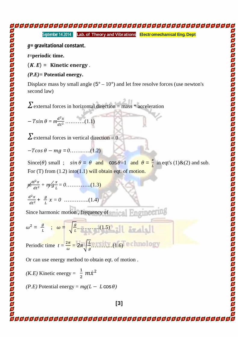
g= gravitational constant.

t=periodic time.

( . ) = .

(P.E)= Potential energy.

Displace mass by small angle (5° – 10°) and let free resolve forces (use newton's second law)

external forces in horizontal direction = mass * acceleration

= m .……….(1.1)

external forces in vertical direction = 0

=0…….…..(1.2)

Since( ) small ; = and cos =1 and = in eqt's (1)&(2) and sub. For (T) from (1.2) into(1.1) will obtain eqt. of motion.

m + m g = 0…………..(1.3)

+ = 0 …………..(1.4)

Since harmonic motion , frequency of

= ; = ..….……..(1.5)

Periodic time t = = 2 …………(1.6)

Or can use energy method to obtain eqt. of motion .

(K.E) Kinetic energy =

(P.E) Potential energy = mg( cos )


[4]

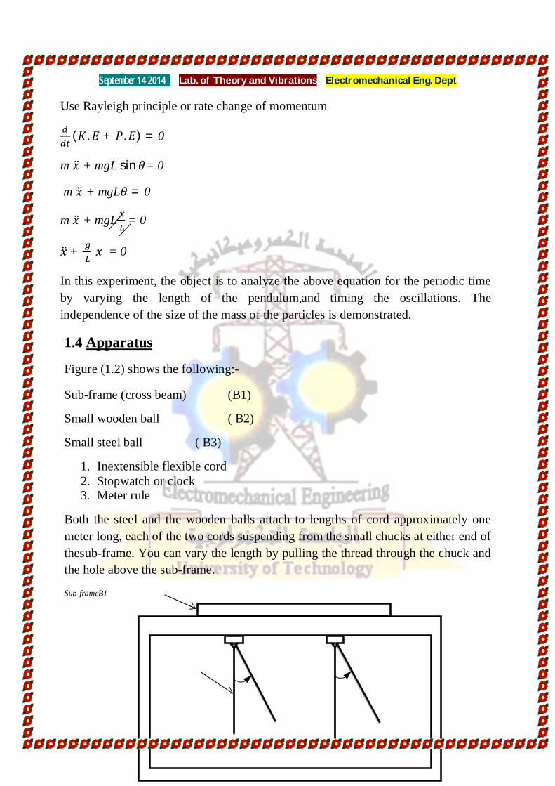
Use Rayleigh principle or rate change of momentum

( . + . ) = 0

m + mgL sin = 0

m + mgL = 0

m + mgL = 0

+ = 0

In this experiment, the object is to analyze the above equation for the periodic time by varying the length of the pendulum,and timing the oscillations. The independence of the size of the mass of the particles is demonstrated.

1.4 Apparatus

Figure (1.2) shows the following:-

Sub-frame (cross beam) (B1)

Small wooden ball ( B2)

Small steel ball ( B3)

1. Inextensible flexible cord 2. Stopwatch or clock 3. Meter rule

Both the steel and the wooden balls attach to lengths of cord approximately one meter long, each of the two cords suspending from the small chucks at either end of thesub-frame. You can vary the length by pulling the thread through the chuck and the hole above the sub-frame.

Sub-frameB1

Inextensible wire

Steel ball B3 B2 Wooden ball


[5]

Frame

Figure (1.2 ) Apparatus of Experiment

1.5 Procedure

Measure and note the lengthL,( the distance from the bottom of the chuck to center of the ball). Displace the pendulum through a small angle and allow swinging freely. Once settled measure the time taken for 50 oscillations and record the periodic time, t.

Repeat the procedure for various values of(L) for both the wooden ball and the steel ball. Enter the result in table (1.1). Plot a graph for values of against values of length L.

1.6 Results

Tablet (1.1) Experiment No. 1 Results

LengthL (m)

Time for 50 complete oscillations

Period t one oscillation Steel

wood

steel wood steel wood


[6]

Figure ( 1.3 ) “against for a simple pendulum”

The graph results in a straight one, giving a relation between ( ) and (L) of the form:

= KL

(slope of line) Where:Kis a constant equal to

Hence the value of g, the acceleration due to gravity, can be determined, also the natural frequency of the system can be obtain experimental for different length (L) and compare with theoretical values for different length.

Discussion of Results1.7

1. What inaccuracies exist in this method for calculating a satisfactory value for (g)?

2. How can you overcome these inaccuracies?

3. Make a comparative study between theoretical and experimental results.

1.8Conclusions


[7]

Experiment No. (2)

MASS - SPRING SYSTEMS

2.1 Object of experiment

1. Determination of helical spring stiffness (K). 2. Determination of natural period of oscillation and obtain natural un damped

frequency. 3. Determination of the effective mass of the spring.

2.2 Introduction

A helical spring, deflecting as a result of applied force, conforms toHooke's Law (deflection proportional to deflecting force).The graph of force against deflection is a straight line as shown in.


[8]

Figure (2.1 )

Slope ofthe line is the 'deflection coefficient' in meters per Newton. The reciprocal of this is the stiffness of the spring and is the forcerequired to produce unit deflection. A rigid body of mass M under elasticrestraint, supported by spring (S), forms the basis of all analysis of vibrationsin mechanical systems.

2.3 Theory of Experiment

M=mass of system

K=spring stiffness

=natural frequency of system.

T = periodic time .

X = deflection.

G = modulus of rigidity.

D = spring diameter.

R = outer diameter of spring.

N = number of spring turns.

= spring mass.

The governing equation of motion for the spring-mass system can be obtained using Newton’s force summation method.


[9]

external forces = mass * acceleration

………….(2.1)

= 0 …………(2.2)

Since system perform harmonic force motion , so can obtain the harmonic oscillating natural frequency .

= …………(2.3)

And periodic time T = 2 .………..(2.4)

2.4 Apparatus

Figure ( 2.2) shows the required set-up for the experiment. Suspend anyone of the three helical springs supplied from the upper adjustableassembly ( )and clamp to the top member of the portal frame.

K

M M

(a) (b) (c)

M x

Equilibrium position

Externalspring forces

inertia forces

kx


[10]

To the lower end of the spring a rod is bolted and integral platform( ) onto which an increment of 0.4kgmass may be added. The rod passes through a brassguide bush, fixed to an adjustable plate ( ), which attaches to the lowermember. A depth gauge is supplied which, when fitted to the uppreassembly withits movable stem resting on the top plate of the guide rod, canbe used to measure deflection, and thereby the stiffness, of a given spring.

Figure ( 2.2 )

2.5 Experiment

( A) (Determination of spring stiffness K)

Fix the specimen spring to the portal frame, with the loadingplatform suspended underneath and the guide rod passing through the guidebush. Carefully adjust the system to ensure that the guide bush is directlybelow the top anchorage point,since any misalignment will produceexperimental errors due to friction. Friction can be minimized by using greaseor oil around the bush.Using the gauge measure the length of the spring with the platformunloaded. Add weights in increments taking note ofthe extension record in Table (2.1),until reaching a suitable maximum load. Remove the Weights, again notingthe length at each increment, as the system unloaded. From these valuesdetermine the mean value of extension for the spring.


[11]

Table (2.1)

Plot a graph for the extension against load, and from this determinethe spring stiffness, k.

2.6 Experiment:

(B)Determination of natural period of oscillation then obtain natural undamped frequency for system.

Add masses-to the platform in varying increments, pull down on theplatform and release to produce vertical vibrations in the system. For eachincrement of Weight note the time taken for 20 complete oscillations record in Table (2.2 )and from this calculate the periodic time, T.

T = 2

Theoretically the periodic time , then natural frequency can be obtained , by calculating the stiffness of spring used from

K = ; G =modulus of rigidity


[12]

Also from known the experimental and theoretical values of natural frequency can obtain the mass of spring

=+

Table (2.2)

Mean coil diameter:

Mean wire diameter:

Number of coil:

M (kg) Time for 20 oscillations

Period T (s) for one oscillation ( )

0

0.4

0.8

1.2

1.6

2.0

Note that =

The mass of the rod and platform are included in (M) above. FromTable (2.2) plot a graph of T against M and find the slope ofthe graph, Figure (2.4)

2.7 Results


[13]

Figure (2.3) Part A graph

0 1.0 2.0 3.0 4.0 5.0 6.0

Mass , M (kg)

Figure (2.4) Part B graph

From the intercept of the line on the M-axis, the effective mass of thespring can be found (m). Compare the value of m obtained with thegenerally accepted value, that

is, mass of spring. Repeat the procedurewith the other springs provided.

Deflection (mm)

4.0 3.0 1.0 Mass , M (kg)

(Square of periodic time of one oscillation)


[14]

2.8 Discussion and Conclusions

1. State your conclusions in the light of the results obtained. Has the basic theory been verified?

2. From the experiments so far performed, discuss the relative merits of each in calculating an accurate value for (T, , ). Criteria for your comments should be:

a) Ease of experimentation. b) Inherent inaccuracies. c) Ease of computation.

3. Choosing some typical results, what error is introduced in calculating (T, , )by neglecting the effective mass of the spring also by considering the spring mass?


[15]

Experiment No. (3)

TORSIONAL OSCILLATIONS OF A SINGLE ROTOR WITH VISCOUS DAMPING

3.1 Object

1. Determining the damping period of oscillation. 2. Determining the logarithmic decrement. 3. Determining the damping coefficient of oil. 4. Determining how damping coefficient depends on the depth immersion of

the rotor in oil. 3.2 Introduction

In This experiment, the effect of including a damper in a system undergoing torsional oscillations is investigated. The amount of damping in the system depends on the extent to which the conical portion of a rotor is exposed to the viscous effects of a given oil. 3.3 Theory

I = mass moment of inertia.

= angular displacement.

K = shaft stiffness.

C = fluid damping coefficient.

= damping period.

=

The equation of the angular motion is: .

Which may be written?

+ + = 0


[16]

Where: = =

The angular displacement is: ( ) = cos ( + )

Where:(U) and ) are constants

The periodic time is: =

Where: is the damped natural freqancy Measuring amplitudes on the same side of the near position, the nth oscillation is

= ( )

Where( ): is a positive integer corresponding to the number of complete oscillations starting at a convenient datum (t=0) Putting ( ) =1 gives the logarithmic

Decrement log = . which is required by basic theory.

3.4 Apparatus

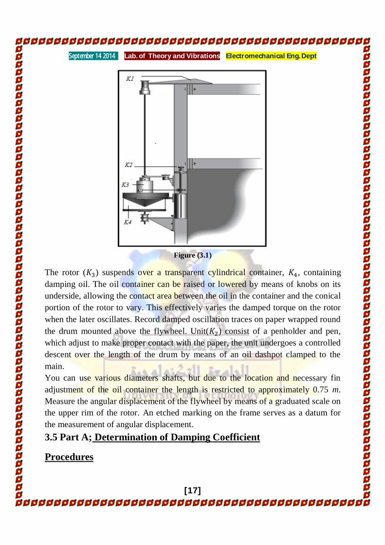
Figure (3.1) shows the apparatus, and consists of a vertical shaft gripped at is upper end by a chuck attached to a bracket ( ) and by a similar chuck attached to a heavy rotor ( ) at its lower end.


[17]

Figure (3.1)

The rotor ( ) suspends over a transparent cylindrical container, , containing damping oil. The oil container can be raised or lowered by means of knobs on its underside, allowing the contact area between the oil in the container and the conical portion of the rotor to vary. This effectively varies the damped torque on the rotor when the later oscillates. Record damped oscillation traces on paper wrapped round the drum mounted above the flywheel. Unit( ) consist of a penholder and pen, which adjust to make proper contact with the paper, the unit undergoes a controlled descent over the length of the drum by means of an oil dashpot clamped to the main. You can use various diameters shafts, but due to the location and necessary fin adjustment of the oil container the length is restricted to approximately 0.75 m. Measure the angular displacement of the flywheel by means of a graduated scale on the upper rim of the rotor. An etched marking on the frame serves as a datum for the measurement of angular displacement. 3.5 Part A; Determination of Damping Coefficient

Procedures


[18]

Fill the cylindrical container K4 with oil to within 10mm of the top.Adjust the knobs underneath to level the oil surface with one of the upper graduations on the conical portion of the rotor, K3.A depth, d of 175mm is suggested for maximum damping. Details of the graduations on the rotor are in Figure(3.2).

Figure(3.2) Conical graduation All dimensions in (mm)

Select and fit a suitable shaft, noting the length of shaft the two inside faces the chuck, together with the diameter of the shaft. Allow the pen to fall, and measure the rate of descent of the pen in ( mm/second) by timing the descent of the pen over a fixed length of paper, using a stopwatch.

The system is now ready for recording torsional oscillations. Raise the pen to the top of the paper on the drum and rotate the rotor to an angle of approximately 40o and then release. A trace of the oscillations can be obtained by bringing the pen into contact with the paper using the thumbnut on the support and allowing the pen to descend.

d=175

d=150

d=100

d=125

d=75

d=50

d=25

G

F

E

D

C

B

A

G

F

E

D

C

B

A

12.5 37.5 62.5 87.5 12.5 50.0 75.0

hi


[19]

Figure(3.3)

Record a trace of the amplitude of oscillation showing decay of vibration due to the damping. The rate of descent of the pen previously carried out will provide suitable time scale. From the trace given in Figure(3.3),measure five successive amplitudes starting with the initial one (n=0) and tabulate the results in Table (3.1) below.

Table (3.1)

n (mm) Logarithmic decrement

( ) = Damping factors


[20]

0 = 1 = 2 = 3 = 4 = 5 =

3.6 Part B; Investigation of How TheDamping Coefficient Depends on The

Depth of Immersion of The Rotor in The Oil

Repeat part A for each oil level as defined by the seven graduation on the conical portion of the rotor.The damping Coefficient depends on the area A of the curved surface of the conical portion of the rotor exposed to viscous damping. This area is equal to , where ( ) is the radius of base of core and ( ) is the slant height equal to + . Plot a graph of damping coefficient to a base of A times mean radius . Tabulate these as in Table (3.2).

Table (3.2)

(mm)

Mean radius ( )

Area A ( )

. ( )

Period ( )

Constant a Damping coefficient

12.5 6.25 25.0 12.50 37.5 18.75 50.0 25.00 62.5 31.25 75.0 37.50 87.5 43.75

3.7 Results


[21]

Plot a graph of log to a base of n. Confirm that the damping is viscous, and

that the slope of the line is equal to ( ) (the logarithmic decrement). The period can be found by timing a convenient number of oscillations using a stopwatch, whereupon the constant, , is determined and hence the value of the damping coefficient (the torque per unit angular velocity) in ( N.m / rad / )

0 100 200 300 400 500

Damping torque per unit angular

velocity

Damping area x effective(mean) radius mm x 10


[22]

Experiment No. (4)

FORCED VIBRATION OF A RIGID BODY – SPRING SYSTEM WITH NEGLIGIBLE DAMPING

4.1 Object of Experiment

1. Determine the natural frequency. 2. Determining the resonance condition. 3. Determining the angular displacement.

4.2Introduction

When external forces act on a system during it’s vibratory motion, it is termed

forced vibration. Under condition of forced vibration, the system will tend to

vibrate at it’s own natural frequency superimposed upon the frequency of the

excitation force.

Friction and damping effects, though only slight are present in all vibrating system;

that portion of the total amplitude not sustained by the external force will gradually

decay. After a short time, the system will vibrate at the frequency of the excitation

force, regardless of the initial conditions or natural frequency of the system.


[23]

4.3Theory

FO sin t

S

D

A CB

L1mg

L

Figure (4.1)

The system is shown in figure(4.1) and comprises of:

1. A beam AB, of length b, sensibly rigid, of mass m, freely pivoted at the left-hand end.

2. A spring of known stiffness S attached to the beam at the point C, at L2 from pivot.

3. A motor with out-of-balance discs attached to the beam at D, at L1 from pivot.

M=mass of the motor including the two discs.

m=mass of the beam.

is the moment of inertia of the system (beam mass+motor and disc) about

the pivot Axis, where:

Mg


[24]

= Angular displacement of the beam;

FO= Maximum value of the disturbing force;

= Angular velocity of rotation to the discs.

L = Total length of beam.

=unbalance mass removed from disc.

The equation of the angular motion can be obtain

By taking moment about pivot (A)

=F0

=M +

The above equation reduces to take the form:

+ = sin t

= e

+ b0 = A

natural frequency = b0 =

= ( ) +3

A = =

Equation solution of motion to give the steady state angular amplitude

. =

=


[25]

Resonance condition

= 0

Note that in practical circumstances the amplitude, although it may be very large, does not become infinite because of the small amount if damping that it always present.

4.4 Apparatus

Figure (4.2)

The apparatus shown in figure 2 consists of a rectangular beam (D6), supported at

one end by a trunnion pivoted in ball bearings located in a fixed housing. The outer

end of the beam is supported by a helical spring of known stiffness bolted to the


[26]

bracket C1 fixed to the top member of the frame. This bracket enables fine

adjustments of the spring, thus raising and lowering the end of the beam.

The DC motor rigidly bolts to the beam with additional masses placed on the

platform attached. Two out-of-balance discs on the output shaft of the belt driven

unit (D4) provide the forcing motion. The forcing frequency adjusts by means of

the speed control unit. The safety stop assembly (D5) limits the beam movement

for safety reasons. It is not a rest for the beam and should not be touching it during

the experiment or the reading will be false.

The chart recorder (D7) fits to the right-hand vertical member of the frame and

provides the means of obtaining a trace of the vibration. The recorder unit consists

of a slowly rotating drum driven by a synchronous motor, operated from auxiliary

supply on the Speed Control unit. A roll of recording paper is adjacent to the drum

and is wound round the drum so that the paper is driven at a constant speed. A felt-

tipped per, fits to the free end of the beam; means are provided for drum adjustment

so that the pen just touches the paper. A small attachable weight guides the paper

vertically downwards. By switching on the motor, we can obtain a trace showing

the oscillations of the end of the beam.

If the amplitude of vibration near to the resonance condition is too large we can

introduce extra damping into the system by fitting the dashpot assembly (pan

numbers D2, D3 and D9) near to the pivoted end of the beam.

4.5 Experimental Procedure

First plug the electrical lead from the synchronous motor into the auxiliary socket

on the Exciter Motor and Speed Control. Adjust the hand wheel of bracket C1 until

the beam is horizontal and bring the chart recorder into a position where the pen

just touches the recording paper. Switch on the speed control unit so the resulting

forced vibration causes the beam to oscillate. lt has been found that a frequency of


[27]

about 2Hz is suitable; the position of the motor can be adjusted accordingly. The

time for 20 oscillations will then be approximately 10 seconds. The chart recorder

can record the number of cycles performed by the beam in a given time (calculated,

knowing the speed of the paper or, better still, by visual counting).

Bring the pen into contact with the paper, then record the number of cycles and

calculate the cycles per unit time {i.e. the frequency) of the forced vibration beam.

You need to known the speed of the paper on the chart recorder. To obtain this,

record a trace for 20 seconds, for example, measure the length of the trace, thus

calculating the speed in mm/s. Determine the values of the relevant parameters as

described in the theory: lengths , magnitude of the masses m and M, also the

stiffness of the spring.

4.6 Results and Calculations

Using a stopwatch, time the linear speed of the drum for 20 vibrations and determine the time for one cycle (period of vibration). Using the two different methods determine the corresponding frequency. Calculate the relevant moment of inertia.

Table (4.1)

Mass of motor with discs, M kg Mass of beam m kg Lengths, L1 m Lengths, L2 m Lengths. L m

Calculate stiffness of the spring as calculated from Experiment No. 1

i.eS = =

Calculate frequency of the forced vibration. The constant:


[28]

b0 =

ƒ = i.e = ( ) cycles

Compare with the values of ƒ found above.

Measure the amplitude of forced vibration (A) from the plot for different exciting (forced) frequency, and compare with theoretical values using derived formula, also at resonance condition ( = ).

4.7 Conclusions

1. Make comparison between measured frequencies (theoretical and experimental) for forced vibration.

2. Make comparison between angular amplitudes. . 3. Measured resonance amplitude with calculated.

Experiment No. (5 )

FORCED DAMPING (UNDAMPED) VIBRATION

5.1 Object

To study the amplitude and phase characteristics of single mass damped system excited by rotating unbalance.

5.2 Theory

m =

beam

0

Beam cross section

2 2

h

b

m


[29]

Figure (5.1) system representation

I = moment of area of beam.

= equivalent mass.

M = removed unbalance mass.

= centrifugal force.

k = beam stiffness.

c=damping coefficient of fluid.

= rotational speed(exciting frequency).

e = eccentricity(distance from center of removed mass to center of

rotation). X = steady state amplitude.

= phase angle.

= damping factor.

= natural frequency.

= critical damping coefficient.

= resonance amplitude.

E = young's modulus of beam material.

b = width of beam.

h = depth of beam.

=12

= + +12


[30]

Equation of motion of the system

( – m) + m(x+c ) = -kx - c

Or; + c + k x = m sin( ) ………….(5.1)

Solution supposed

= X sin( ) …………..(5.2)

Where ; unknown amplitude , ; unknown angle of phase lag .

5.3 Analytical Representation

After substituting (5.2) into (5.1) we get ;

X ( ) + c X cos ( ) + k X ( )

=m sin( )

= ( )

X ( )+ c X ( + ) + k X ( )= m sin( ) ……….....(5.3)

5.4 Vector (Graphical) Representation

Y

X

C

m

kX


[31]

X

Figure (5.2 )Vector Representation

From the figure (5.2) can obtain

X=( )

; tan =

knowing that ; = ; = ; = 2 and = 2

= ( )

( ( ) ) ( )…………(5.4)

and; tan =( )

.…………(5.5)

in resonance =

= , = .….………..(5.6)

5.5 Equipment used

1. Rectangular beam simply supported. 2. Small motor with two graduated unbalance discs. 3. Stroboscope. 4. Micrometer. 5. Motor speed control unit. 6. Dashpot. 7. Contractor.

5.6 Procedure


[32]

1. For forced undamped vibration, remove dashpot. 2. Run the motor to a certain speed by the speed control unit. 3. At each speed measure the amplitude of vibration and the phase lag at the

instant when the earthed micrometer and the contactor are in contact (the first stroboscope flash).

4. Repeat (3) at various speeds. 5. Repeat 2, 3, 4 with dashpot.

5.7 Requirements

1. Determine the equivalent mass;

= + +12

2. Determine the stiffness at = 2 ,k= =

3. Determine theoretical natural frequency ; =

4. Measure and plot amplitude phase characteristics of investigated system. 5. Knowing , determine according to equation (6) 6. Knowing and corresponding verify

E=2.1*10 2 , L=80 cm , M=8 Kg , b=2.54 cm , D=1.5 cm (dia.of beam cross section )

=2.8*10 3 , t= 7 mm , e=4 cm , d=2 cm , h=1.27 cm

5.8 Discussion

1. Discuss the effect of ( ) on the amplitude and phase angle . 2. Discuss your results. 3. Discuss the effect of unbalance of the vibration. 4. State the advantages of oil on damping vibration. 5. State the application of vibration absorber.


[33]

Experiment No.(6)

Torsional Oscillations of Two Rotor System

Object of Experiment6.1

Determination of following:


[34]

1. moment of Inertia of rotors disc.

2. torsional stiffness of shaft.

3. natural period of oscillation of the two degree of freedom system.

Introduction6.2

Figure (6.1)

Systems that require two independent coordinates to describe their motion are called two degree of freedom system. The general rule for the computation of the number of degree of freedom can be stated as follows

So there are two equations of motion for a two degree system ,one for each degree they are generally in the form of coupled differential equations in values all the coordinate ,the equations of motion lead to a frequency equation that give two natural frequencies for the system. Thus a two degree system has two normal modes of vibration corresponding to the two natural frequencies .In multi degree of corresponding to the two natural frequencies .In

Number of degree of freedom of the system

Number of masses in the system ×number of possible types of motion of each mass

=


[35]

multi degree of freedom systems there is semi definite systems which known unstrained or degenerate systems in this case we have two degree System an two masses connected by spring { e.g (1) two railway cars, (2)turbine and air blower connected by shaft ,( 3) gear train}

It can be seen from solution of frequency equation that one of natural frequencies of the system is zero ,which means that the system is not oscillating .In other word the system as a whole without any relative motion between the two masses (rigid body translation).

Theory6.3

= Moment of inertia of rotor 1

=

L=Length of the shaft between the rotors

G= Modulus of rigidity of the material of the shaft

J=Polar second moment of area of the shaft section

=torsional stiffness of shaft.

1, 2) = angular displacement of rotors. = ( i=

Using summation of moment method… (Newton2nd law) External moment =

= ( ) .………..(6.1)

in

out gear

k

gear in mesh.


[36]

( ).………. (6.2) + =0……….….(6.3)

+ =0……….….(6.4)

Figure (6.2) Two degree of freedom torsional system

Assumed solution

( ) =

( )

[( ) ] = 0

[(

( )

To find natural frequencies to determinate of matrix.

( )( ) = 0 …….….(6.6)

[ ( + )] = 0 …….….(6.7)

L

…….… (6.5)


[37]

either = 0 or = ( )……..…(6.8)

= ( )rad/sec

Even it is two degree of freedom system but one can notice only one frequency because the system is degenerated.

The period of oscillation

= And using ( ) =

Then: = 2 1 2

( 1+ 2

This period can be calculate and compared with that obtained from the experimental values, also the value of obtained theoretically be compared with the experimental from previous experiments, and the mass moment of inertia of each disc can be compared from results.

6.4 Experimental procedure

One of the shafts clamps between the two rotors of predetermined inertia. Record the effective length of the shaft measured between the jaws of the chucks to insure that neither rotor can slip relative to the shaft. Rotate each rotor through a small angle in opposite directions and then release torsional oscillations of the system are thereby set up and the time for 20 oscillation recorded.

The periodic time of the system may be determined and compared with the theoretical value given by the formula quoted in the theory section determine the moment of inertia of each by measuring the time for 20 oscillation ,This system is a single degree of freedom.


[38]

When the frequency of oscillate can be obtain from

=( )

,then to obtain the moment of inertia from

= 2 =2

=

So

=4

6.5 Results and discussion

Obtain the period of oscillation for the system for certain number of Oscillation for different diameters and length of shafts and arrange in table and obtain the theoretical values using the equation for period and make comparison and discuss the effect of varying the length and diameter.

Also material (G) and state why there are differences and give reasons.

Theoretical value of period

Period Sec

Time for 20 oscillation

Shaft diameter

mm 3.17

4.76

6.35


[39]

ExperimentNo.(7)

CRITICAL WHIRLING SPEED OF SHAFT

7.1 Introduction

For any rotating shaft, a certain speed exists at which violent instability occurs. The shaft suffers excessive deflection and bows – a phenomenon known as “whirling” .

If this “critical speed of whirling” is maintained, then the resulting amplitude becomes sufficient to cause buckling and failure. However, if the speed is rapidly increased before such deleterious effects occur, then the shafts is seen to re-stabilize and run true again until, at another specific speed, a double bow is produced and so on for other speeds

Dunkerley first investigated the centrifugal forces involved and determined that the only stabilizing force was that due to the elastic properties (“stiffness”) of the shaft. Hence, he was able to deduce the speed at which the shaft would suffer an infinite deflection due to whirling

7.2 Object of Experiment

An accurate analysis of the critical whirling speed for the range of shaft geometry’s, both loaded and unloaded and with different combinations of end conditions.

7.3 Description of apparatus

The whirling of shaft apparatus is shown in Figure (7.1)two unique features are incorporated, which allow the shaft to adopt its actual whirling configuration predicted by elastic theory. The first is a kinematic coupling located at the driven


[40]

end of the shaft, which is designed to prevent the transmission of any restraining forces by the motor of the shaft. The second features is a sliding bushed end which affords sliding motion of the shaft on a longitudinal phosphor bronze bearing , whilst revolving in a radial ball bearing.

A diagrammatic representation of the whirling of shafts apparatus is shown in figure (7.1.a). The specimen shaft is of the form shown infigure (7.1.b) and is located in the kinematic coupling and either the fixed or free type sliding end bearing. Several shafts of various diameters and lengths are available and these appear tabulated in the table (7.1).

(a)

(b)

Figure (7.1) whirling of shaft apparatus (a) and shaft (b)

Table (7.1) Shaft Diameters and Lengths Available

Shaft No. d mm

m


[41]

1. 2. 3. 4.

3 3 6 7

0.750 0.900 0.900 0.900

The Kinematic coupling and sliding end bearings have been so designed as to allow the shaft movement in a longitudinal direction, for the purpose of location before tightening, and so provide directional clamping of the shaft end.With the standard apparatus, the sliding end bearing provides directional fixing to the end of the shaft, although an interchangeable sliding end bearing is available which provides a directionally free support. These bearings are showninfigures (7.2) and (7.3).


[42]

7.4 Theory

= Natural frequency of transverse vibration mode

E= Young's modulus

= Second moment of area of shaft

= Weight per unit length of shaft

2

Figure (7.3) sliding bearing (directionally free)

Figure (7.2) sliding bearing (fixed)


[43]

= Acceleration due to the gravity

= Constant dependent upon the end conditions and mode number

d = shaft diameter

=shaft length

A = amplitude

M = disc mass

= eccentricity

K = shaft stiffness

= exciting speed

= critical speed

= weights

= constants

If we examine the simplest case of a single, heavy rotor rigidly attached to a light (inertia-less) spindle, then the physical situation can be expressed in Figure (7.4)

Figure (7.4) whirling of shaft due to unbalance

G

C

A

O O D


[44]

The system consists of a disc of mass (M) located on a shaft simply supported by two bearings. The center of gravity (G) of the disc is at a radial distance from the geometric centre C. The centre line of the bearings OO intersects the plane of the disc at D, at which point the disc center C is deflected a distance A

The centre of gravity G thus around point D, describing a circle radius ( + ) and the centrifugal reaction thus produced is:

(A+ ) ………….(7.1)

For any given speed

This force, according to Dunkerley, is balanced by elastic righting forced of the shaft at point D equal to KA where K is stiffness of supported shaft.

Therefore

( + ) = …………… (7.2)

From which, the amplitude of vibration obtained

= …………… (7.3)

This equation will become infinite when = 0

(i.e resonance condition)

= …………. (7.4)

Therefore, if denotes the critical whirling speed, substituting in equation (7.3)

the value of = , we obtain

= ………….. (7.5)

Therefore, at < then A and have the same sign, i.e. the centre of gravity G is situated as shown in Figure (7.4).


[45]

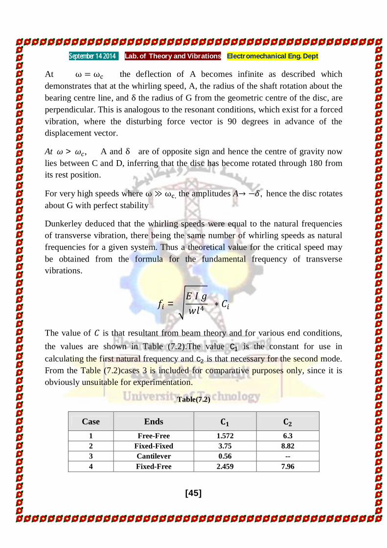
At the deflection of A becomes infinite as described which demonstrates that at the whirling speed, A, the radius of the shaft rotation about the bearing centre line, and the radius of G from the geometric centre of the disc, are perpendicular. This is analogous to the resonant conditions, which exist for a forced vibration, where the disturbing force vector is 90 degrees in advance of the displacement vector.

At > , A and are of opposite sign and hence the centre of gravity now lies between C and D, inferring that the disc has become rotated through 180 from its rest position.

For very high speeds where , the amplitudes A , hence the disc rotates about G with perfect stability

Dunkerley deduced that the whirling speeds were equal to the natural frequencies of transverse vibration, there being the same number of whirling speeds as natural frequencies for a given system. Thus a theoretical value for the critical speed may be obtained from the formula for the fundamental frequency of transverse vibrations.

=

The value of is that resultant from beam theory and for various end conditions, the values are shown in Table (7.2).The value c is the constant for use in calculating the first natural frequency and c is that necessary for the second mode. From the Table (7.2)cases 3 is included for comparative purposes only, since it is obviously unsuitable for experimentation.

Table(7.2)

Case Ends 1 Free-Free 1.572 6.3 2 Fixed-Fixed 3.75 8.82 3 Cantilever 0.56 -- 4 Fixed-Free 2.459 7.96


[46]

Table of constants to Calculate Frequency of Transverse Vibration for various End Conditions.

7.5 Results and discussion

The experimental result of speeds for each of above cases are carried out and each one been noted from the digital recorder, and verified by the stroboscope image of the specific mode as shown in Figure (7.5),(7.6).

Figure (7.5)


[47]

Which shows the first and second whirl mode .these values can be compared with the theoretical ones for each boundary conditions ,the difference between them is due two experiment environment.. etc

7.6 Conclusions:-

1. What can you deduce from the increase in speed on, shape… 2. Effect of boundary conditions on shapes and critical speed values.

Figure (7.6)


[48]

ëuotechnology.edu.iq/dep-electromechanic/typicall/lab/folder/theory... · 7. critical whirling...

Documents