vtechworks.lib.vt.edu~ geometrically nonlinear finite element analysis of space frames by ‘ jih...
TRANSCRIPT

GEOMETRICALLY NONLINEAR FINITE ELEMENT ANALYSIS
OF SPACE FRAMES
by
Jih JihhJau„
Dissertation submitted to the Faculty of the
Virginia Polytechnic Institute and State University
in partial fulfillment of the requirements for the degree of
DOCTOR OF PHILOSOPHY‘ in
Civil Engineering
APPROVED:
"ÄS(’Holzer, Cha rman
R. . Barker T. Ku pus y
M. P. Singh A. E. Somers
February, 1985‘
Blacksburg, Virginia
~Geometrically Nonlinear Finite Element Analysis
of Space Frames
by‘ Jih Jih Jau
(ABSTRACT)
The displacement method of the finite element is
adopted. Both the updated Lagrangian formulation and total
Lagrangian formulation of a three-dimensional beam element
is employed for large displacement and large rotation, but
small strain analysis.
A beam-column element or finite element can be used to
model geometrically nonlinear behavior of space frames. The
two element models are compared on the basis of their
efficiency, accuracy, economy and limitations.
An iterative approach, either Newton-Raphson iteration
or modified Riks/Wempner iteration, is employed to trace the
nonlinear equilibrium path. The latter can be used to
perform postbuckling anaylsis.

. ACKNOWLEDGEMENTS
The author would like to express his sincere appreciation
to Dr. S. M. Holzer for his guidance, encouragement and in-
finite patience. The author is also very much obliged to Dr.
R. M. Barker, Dr. T. Kuppusamy, Dr. M. P. Singh and Dr. A.
E. Somers for reviewing this dissertation, giving advice and
serving on the committee.
Finally, the author gives deep gratitude to his beloved
family for their complete devotion and encouragement.
iii
TABLE OF CONTENTS
ABSTRACT ........................ ii
ACKNOWLEDGEMENTS ................... iii
Chapterpage
I. INTRODUCTION ................... 1
Purpose and Scope ............... 1Survey of Literature ............. 3
V II. UPDATED AND TOTAL LAGRANGIAN FORMULATIONS INGEOMATRICALLY NONLINEAR FINITE ELEMENTANALYSIS .................. 7
Introduction ................. 7Incremental Equilibrium Equation in U.L.
Formulation ............... 11Incremental U.L. Continuum Mechanics
Formulation ............. 11Incremental Strain ............. 15Incremental Equilibrium Equation ...... 17Transformation Matrix ........... 25
Incremental Equilibrium Equation in T.L.Formulation ............... 28
Incremental T.L. Continuum MechanicsFormulation ............. 28
Incremental Strain ............. 31Incremental Equilibrium Equation ...... 32Transformation Matrix ........... 37
Convected Coordinate Formulation ....... 4OComparison of U.L. and T.L. Formulations . . . 46
III. DEFORMATION DISPLACEMENTS OF SPACE FRAME ELEMENT . 54
Introduction ................. 54Coordinate System of Space Frame ....... 55Nodal Displacements .............. 57Element Deformation Displacements ....... 61
IV. FINITE ELEMENT MODEL ............... 7O
Introduction ................. 7O
iv
Interpolation Functions for IncrementalDisplacements .............. 71
· Linear Strain Incremental Stiffness Matrix . . 74Nonlinear Strain Incremental Stiffness Matrix . 75Local Strain Incremental Stiffness Matrix . . . 76Global Strain Incremental Stiffness Matrix . . 77Local Element Forces ............. 81Global Element Forces ............. 88
V. BEAM-COLUMN MODEL ................ 90
Introduction ................. 90Element End Force-Deformation Relations .... 91Tangent Stiffness Matrix for Relative
Deformations .............. 94Local Element Tangent Stiffness Matrix .... 95Global Element Tangent Stiffness Matrix . . . 101
VI. SOLUTION ALGORITHMS .............. 106
Introduction ................ 106Newton—Raphson Method ............ 107Modified Riks/wempner Method ........ 111Convergence Criteria ............ 114
VII. SAMPLE ANALYSIS .............. , . 118
Introduction ................ 118Example 1: Williams' Toggle Frame ...... 118Example 2 : Three Dimensional Cantilever Beam
of a 45-Degree Bend .......... 119Example 3: 12 Member Model Frame ...... 130Example 4: Reticulated Dome ......... 131
VIII. PROGRAM DEVELOPMENT .............. 143
Introduction ................ 143Program Structure .............. 144
Main Program ............... 144Subroutine DATA ............. 147Subroutine STRUCT ............ 148Subroutine CODES ............. 149Subroutine DETMAX ............ 150Subroutine PROP ............. 152Subroutine LOAD ............. 154Subroutine JLOAD ............. 155Subroutine NEWRAP ............ 156Subroutine RIKWEM ............ 159Subroutine STIFF ............. 163Subroutine ELEMS1 ............ 165
v
Subroutine ELEMS2 ............ 167a
Subroutine ASSEMS ............ 169Subroutine STORE ............. 170Subroutine FORCES ............ 171Subroutine ELEMF ............. 174Subroutine BOWCOR ............ 177Subroutine RESULT ............ 180Subroutine JOINTF ............ 181Subroutine OUTPUT ............ 182
IX. CONCLUSION ................... 184
Conclusion ................. 184Suggestions for Future Development ..... 188
REFERENCES ...................... 190
Apgendixpage
A. JOINT ORIENTATION MATRIX FOR SMALL JOINTROTATIONS ................ 196
B. STABILITY FUNCTIONS .............. 203
C. GEOMETRIC MATRICES gi ............. 205
D. g(if = AT §(i)A ................. 207
E. NOTATION .................... 209
F. PROGRAM LISTING ................ 222
VITA ................................................... 261
vi
LIST OF FIGURES
Figurepage
2.1.Motion of an Element in Cartesian Coordinate System 9
2.2.Loca1 Element Displacements in U.L. formulation forPlane Frame ................... 23
2.3.Local Element Forces and Displacements in SpaceFrame ...................... 26
2.4.Global Element Forces and Displacements in SpaceFrame ...................... 27
2.5.Local Element Displacements in T.L. Formulation forPlane Frame ................... 38
2.6.Local Element Displacements in Convected CoordinateFormulation for Plane Frame ........... 42
3.l.Coordinate System of Space Frame .......... 56
3.2.Incrementa1 Nodal Rotations ............ 60
3.3.Element Deformation Displacements and AssociatedForces ..................... 64
4.l.Local and Natural Coordinate Systems ........ 73
4.2.Deformation Displacements and Forces in xl-x2 Plane 83
4.3.Deformation Displacements and Forces in xl—x3 Plane 84
4.4.Relative Element Forces and Displacements in SpaceFrame Element .................. 87
5.1.The Relative Member End Deformations and AssociatedForces in Space Frame .............. 93
5.2.Basic Local Element Forces Associated with Oran‘sBeam—Column Model in Space Frame ........ 97
6.l.Newton—Raphson Iteration ............. 109
6.2.Modified Newton—Raphson Iteration ........ 110
vii
6.3.Modified Riks/Wempner Iteration along the NormalPlane ..................... 115
6.4.Iteration Prodedure along Normal Plane with UpdatingK ....................... 116
7.1.Williams' Toggle Frame .............. 120
7.2.Finite Element Model ............... 121
7.3.Comparison of Models ............... 122
7.4.Three Dimensional Cantilevel Beam of 45-Degree Bend 123
7.5.Finite Element Model ............... 125
7.6.Beam—Column Model ................ 126
7.7.Comparison of Models ............... 127
7.8.Load Deflection Curves .............. 128
7.9.Deflected Shapes of a 45-Degree Circular Bend usingthe Beam-Column Model ............. 129
7.10.12 Member Model Frame .............. 132
7.11.Finite Element Model .............. 133
7.12.Beam—Column Model ................ 134
7.13.Comparison of Models .............. 135
7.14.Load Deflection Curves ............. 136
7.15.Load Deflection Curves ............. 137
7.16.Reticulated Dome ................ 139
7.17.Finite Element Model .............. 140
7.18.Beam-Column Model ..............·. . 141
7.19.Comparison of Frame Dome with Truss Dome .... 142
8.1.Program Structure ................ 146
A.1.Smal1 Joint Rotation ............... 199
A.2.Small Joint Rotation P2 about X2—axis ...... 200
viii
A.3.Smal1 Joint Rotation P3 about b3-axis......201
A.4.Small Joint Rotation P1 about al-axis......202
ix
Chapter I
INTRODUCTION
1.1 PURPOSE ggg ggggg
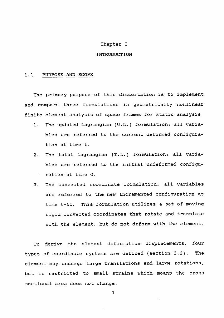
The primary purpose of this dissertation is to implement
and compare three formulations in geometrically nonlinear
finite element analysis of space frames for static analysis
1. The updated Lagrangian (U.L.) formulation: all varia-
bles are referred to the current deformed configura-
tion at time t.
2. The total Lagrangian (T.L.) formulation: all varia-
bles are referred to the initial undeformed configu-
‘ ration at time O.
3. The convected coordinate formulation: all variables
are referred to the new incremented configuration at
time t+At. This formulation utilizes a set of moving
rigid convected coordinates that rotate and translate
with the element, but do not deform with the element.
To derive the element deformation displacements, four
types of coordinate systems are defined (section 3.2). The
element may undergo large translations and large rotations,
but is restricted to small strains which means the cross
sectional area does not change.
1
2
The second purpose is to compare two models of geometri-
cally' nonlinear space frames. To predict the structural
response accurately, it is necessary to select the proper
mathematical models, either finite element model or a beam-
column model can be used. The finite element model is for-
mulated by the principle of virtual work with Lagrangian and
Hermitian interpolation functions used for discretization.
The beam-column model, developed by Oran [l], [2], [3], is
based on the conventional beam-column theory.
The solution procedure is iterative as well as incremen-
tal. The Newton-Raphson method and the modified kiks/Wemp-
ner method [27] are employed. The Newton-Raphson method can-
not be used to trace equilibrium path beyond the limit
point; for this reason the modified Riks/Wempner method was
developed.
The final purpose is to develop a computer program for
geometrically nonlinear static analysis of space frames. The
U.L. formulation was implemented in this program. Several
test examples were investigated using the computer program.
The results compared well with available data in the litera-
ture.

3
1.2 SURVEY Q; LITERATURE
The analysis of geometrically nonlinear framed structures
has attracted considerable attention during the last two de-
cades. An early paper by Connor [16] presented a nonlinear
formulation for a rigid-jointed space frame with small rota-
tions subjected to loads applied only at the joints. Oran
[1], [2], [3] derived a tangent stiffness matrix for elastic
frame structures based on the conventional beam-column theo-
ry [23] in which small relative deformations of the members
were assumed, however the rotations and translations of the
joints were considered to be arbitrarily large. Belytschko
and coworkers [5],[17] employed a convected coordinate sys-
tem in which the deformation displacements were seperated
from the rigid body motion, and node orientations were de-
scribed by unit vectors that only three components of two
unit vectors were stored. Mikkola [4] combined Oran's and
Belytschko's formulations in which joint displacements and
element deformations were described, and derived the tangent
stiffness matrix in the different form.
A large displacement problem in structural analysis can
be analyzed in three types of formulationsz U.L., T.L. and
convected coordinates formulations.

4
References [25],[26],[39],[4l] adopted the U.L.
formulation: Murray and Wilson [25],[4l] investigated the
response of thin elastic plates and employed in-plane dis-
placement functions and plate bending displacement functions
which maintained boundary compatibility for the in-plane and
bending problems, respectively, but violated boundary compa-
tibility when superimposed in the large deflection problem.
Yang [26] applied a linearized midpoint tangent incremental
approach to predict the nonlinear equilibrium path. Chu and
coworkers [39] developed the constant load method to deter-
mine buckling loads of space frames based on the large de-
flection theory in which the iteration may start at any load
level and the stiffness matrix developed for small deflec-
tion theory could be used directly.
References [7],[l2],[l9],[20],[32] adopted the T.L. for-
mulation: Rajasekaran and Murray [7] showed that the equi-
librium equation and the linear incremental equilibrium
equation did not necessarily follow from the total potential
energy in the form introduced by Mallett and Marcal [8], and
derived the particular forms of the incremental stiffness
matrices. Hibbitt and coworkers [12] developed a large dis-
placement, large strain formulation by introducing an addi-
tional initial load stiffness matrix into the large dis-
- 5
placement, small strain formulation, and took the material
to be elastic-plastic. Remseth [19],[32] presented nonlinear
static and dynamic analysis of space frames in which the
node rotations were limited to 12 to 15 degree, and higher
order axial interpolation polynomials were included in order
to obtain an appropriate coupling between axial forces and
bending. Wood and Zienkiewicz [20] presented the geometri-
cally nonlinear analysis of the two dimensional inplane
structures, e.g. beams,frames and arches, which omitted mid-
side nodes in the "thickness" direction, thereby reducing
the number of degrees of freedom, and employed a paralinear
isoparametric element.
Cook [33] gave an basic introduction to the geometric
nonlinear problem. Bathe [9],[10],[38] presented an U.L. and
a T.L. formulation, derived from the continuum mechanics, of
space frame element for large displacement analysis. Tang
[18] described these three formulations and explained that
in the convected coordinate formulation an incremental con-
cept was impracticable, thus the tangent stiffness matrix
was difficult to be established.
Wood and Schrefler [6] gave a correlation between the
so—called N—notation and the B—notation of the T.L. formula-
6
tion of geometrically nonlinear problems. Mallet [8] and Ra-
jasekaran [7] adopted the N-notation, Zienkiewicz and co-
workers [3l], [20] adopted the B—notation.
Katzenberger [48] derived the secant stiffness matrices
for the plane frame element from which element forces can be
obtained. Butler [29] compared two models for geometrically
nonlinear finite element analysis of plane frames.
To trace nonlinear equilibrium paths into the postbuck—
ling range, Holzer [27] employed the modified Riks/Wempner
method. Bathe and Cimento [49] described the practical
procedures for the incremental solution of nonlinear finite
element equations and proposed specific ways to measure con-
vergence.
Papadrakakis [21] employed the vector iteration methods
to study the post—buckling behavior of spatial structures in
which there is no need to compute or formulate the tangent
stiffness matrix.
Chapter II
UPDATED AND TOTAL LAGRANGIAN FORMULATIONS INGEOMATRICALLY NONLINEAR FINITE ELEMENT ANALYSIS
2.1 INTRODUCTION
Large displacement analysis may be formulated in three
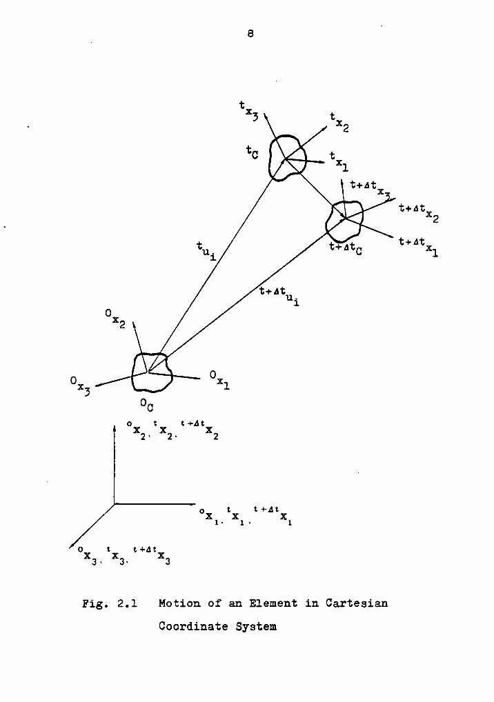
types of coordinate systems (Fig. 2.1):
1. The total Lagranginan (T.L.) formulation which refers
to the initial undeformed equilibrium configuration
Oc at time O.
2. The updated Lagrangian (U.L.) formulation which re-
fers to the current deformed equilibrium configura-
tion tc at time t.
3. The convected coordinate (Eulerian) formulation which
refers to the new incremented configurationt+AtC at
time t+At.
In Fig. 2.1 0Xi, tXi, t+AtXi are the global coordinate
systems in the configuration at time O, t, t+At respective-
ly, i=l, 2, 3; Oxi, txi, t+Atxi are the local coordinate
systems at time O, t, t+At respectively;tui, t+Atui
are the
displacement components from initial position at time O to
configuration at time t, t+At respectively.
4 7
t
· 2
tc tX1t+Atx
t+At. X2
t+Ati
t+Atui
OX2
OO xx3 lOc
ox tx t +AtX2- 2· 2
Qx SX I +ÄIX1 · 1 - 1
Ox IX t +AtX3- 3· 3
Fig. 2.1 Motion of an Element in Cartesian
Coordinate System
9
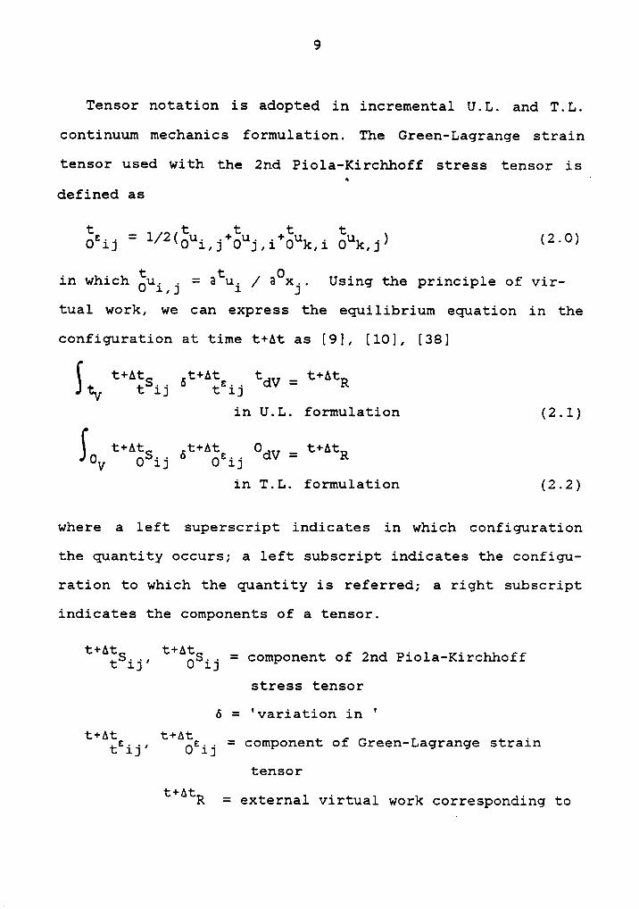
Tensor notation is adopted in incremental U.L. and T.L.
continuum mechanics formulation. The Green—Lagrange strain
tensor used with the 2nd Piola-Kirchhoff stress tensor is
defined as
t _ t t t tOsij i Ouklj) (2.0)
. . t _ t O . . . .in which Oui j— 8 ui / 8 xj. Using the principle of v1r-
tual work, we can express the equilibrium equation in the
configuration at time t+At as [9], [10], [38]
t+At t+At t _ t+AtStv tSij 6 tsij dV — R
in U.L. formulation (2.1)
S t+At t+At 0 _ t+AtOV 0Sij 6 Osij dV — R
in T.L. formulation (2.2)
where a left superscript indicates in which configuration
the quantity occurs; a left subscript indicates the configu-
ration to which the quantity is referred; a right subscript
indicates the components of a tensor.
component of 2nd Piola-Kirchhoff
stress tensor
6 = 'variation in 't+A;sij,
t+Aäsij = component of Green-Lagrange strain
tensort+At _ . .
R — external virtual work corresponding to
10
configuration at time t+At
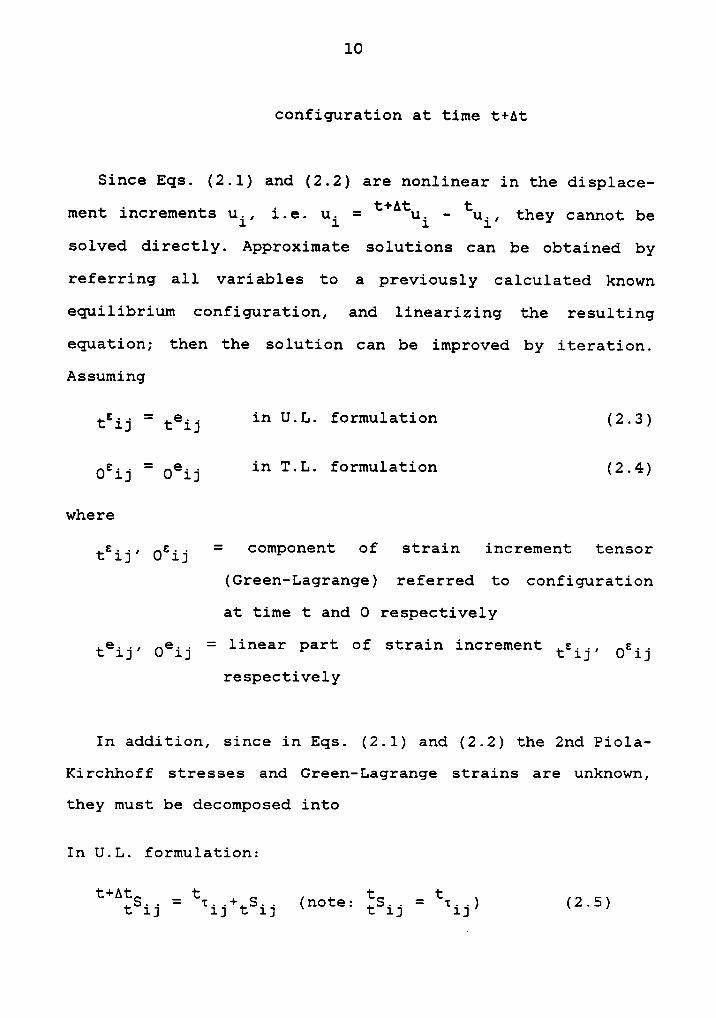
Since Eqs. (2.1) and (2.2) are nonlinear in the displace-
ment increments ui, i.e. ui = t+Atui — tui, they cannot besolved directly. Approximate solutions can be obtained bY
referring all ·variables to a previously calculated known
equilibrium configuration, and linearizing the resulting
equation; then the solution can be improved by iteration.
Assuming
ttij = teij in U.L. formulation (2.3)
Osij = Oeij in T.L. formulation (2.4)
where
tsij, Osij = component of strain increment tensor
(Green—Lagrange) referred to configuration
at time t and O respectively
teij, Oeij = linear part of strain increment tsij, Osij
respectively
In addition, since in Eqs. (2.1) and (2.2) the 2nd Piola-
Kirchhoff stresses and Green-Lagrange strains are unknown,
they must be decomposed into
In U.L. formulation:
t+At _ t _ t _ ttSij - 1ij+tSij (note. tSij - rij) (2.5)
11
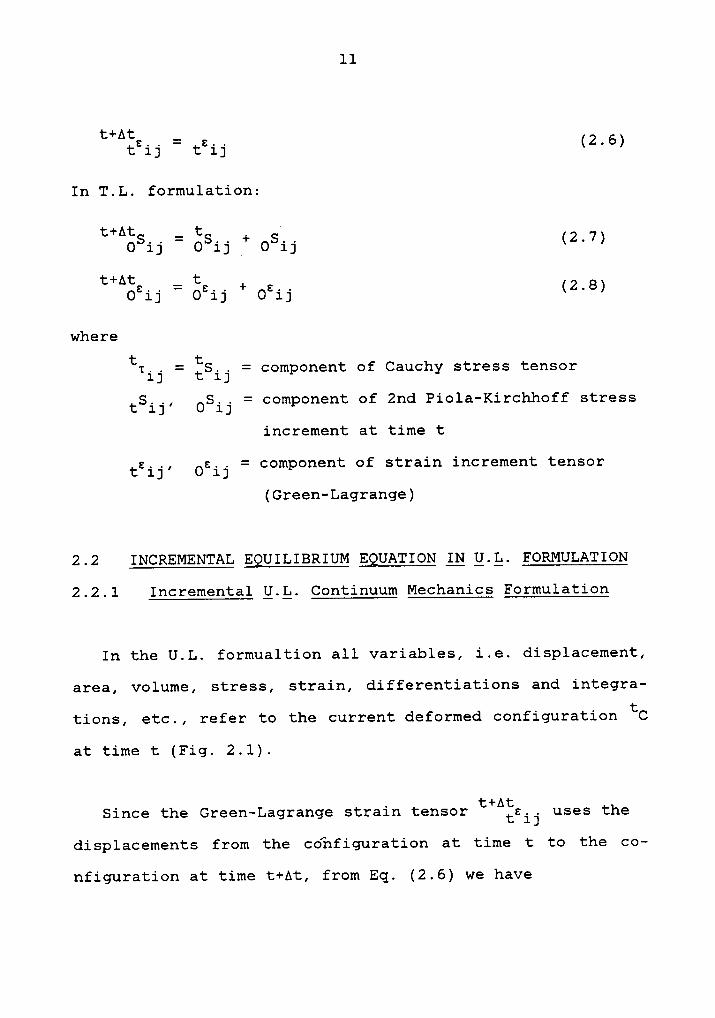
t+Attsij = tzij (2.6)
In T.L. formulation:
t+At _ t0Sij - 0Sij + 0Sij (2.7)
t+At _ tOsij
— Osij + Osij (2.8)
wheret _ t _rij —
tSij - component of Cauchy stress tensor
tSij, 0Sij = component of 2nd Piola-Kirchhoff stress
increment at time t
tsij, Osij = component of strain increment tensor
(Green-Lagrange)
2.2 INCREMENTAL EQUILIBRIUM EQUATION IQ Q.g. FORMULATION
2.2.1 Incremental Q.g. Continuum Mechanics Formulation
In the U.L. formualtion all variables, i.e. displacement,
area, volume, stress, strain, differentiations and integra-
tions, etc., refer to the current deformed configurationtc
at time t (Fig. 2.1).
. . t+AtSince the Green-Lagrange strain tensor tsij uses the
displacements from the configuration at time t to the co-
nfiguration at time t+At, from Eq. (2.6) we have
12
t+At _6 tcij
— ötsij (2.9)
Substituting Eqs. (2.5), (2.9) into Eq. (2.1) yields
t t t _ t¥AtStv rij ötsij dV + j;v_tSij ötsij dV - R (2.10)
The strain increment components can be separated into li-
near and nonlinear parts
615 = $15‘“
913 (L11)
where
e.. = „t 13 1/2 (tuilj + tuj’i) (2.12)
tnij = 1/2 tukli tuk j (2.13)
u = au /atx
(2 14)t 1.5 i 5 '_ t+At _ t _ .=ui — ui ui , 1 1,2,3 (2.15)
tnij is the nonlinear part of strain increment ésij; tui jis the derivative of displacement increment with respect to
local coordinate txj; uiare the increments in the displace-
ments from time t to time t+At; tui, t+Atui are the dis-placement components in the local coordinate system from the
initial configuration at time 0 to the deformed configura-
tion at time t and time t+At respectively.
13
tui = txi — Oxi (2.15a)t+At _ t+At 0ui — xi xi (2.15b)
t t+At . . . .where ui and ui are the functions of position coord1—
nates (xl, x2, x3) respectively.
The constitutive law is [10]
615 = tcijrs 61-5 (266)
where tCijrS is the component of incremental material prop-
erty tensor at time t referred to the configuration at time
t.
Using Eqs. (2.11), (2.16), Eq. (2.10) can be transformed to
t t tStvtC15tS 61·s 6615 dv * Stv *15 6615 dv
_ t+At _ t t— R Stv tij öteij dV (2.17)
Eq. (2.17) is nonlinear in the incremental displacements ui,
and it can be linearized by using the approximations
ötsij = öteij (2.18)
tsij = tcijrs ters (2°19)
Therefore Eq. (2.17) becomes
t t t,ttvtC151~s ttm 6615 dv 6 Stv *15 6615 dv
_ t+At t t- R Stv tij öteij dV (2.20)
14
Eq. (2.20) is the incremental equilibrium equation of a
deformed element, linear in the incremental displacements
ui, corresponding to the local coordinate system.
In three dimensional beam element for our problem, small
deformation and uniaxial state of strain (i.e. tell only)
are assumed, and torsion is treated independently from bend-
ing and axial force so that it can be obtained from linear
theory; in this situation Eq. (2.20) can be specialized as
t 5 t tEjtvtell ötell dV + tv ¤ ötnll dV
_ t+At _ t t- R ugtv c ötell dV (2.21)
whereV
= 2.22E tcllll ( )t¤ = tell (2.23)
E is the Young's modulus and to is the axial Cauchy stress.
Eq. (2.21) can be expressed in matrix form. By using in-
terpolation functions for incremental displacements to eval-
uate the derivatives of displacements, we will obtain the

15
linear and nonlinear strain-displacement transformation ma-
trices. For a beam element it is more effective to first
evaluate the finite element matrices in the local coordinate
axes xi, and then transform them to the global coordinate
axes Xi prior to the element assemblage process.
2.2.2 Incremental Strain
For our uniaxial strain problem, the ui in Eq. (2.15) me-
ans the displacement increments along the centroid axis of
elements and is only the function of xl-axis. By using in-
terpolation function, ui can be expressed in the nodal dis-
placement increments.
·A
Atdl
Atdz
tu? . 0 thz 0 0 0 ths E 0 th8 0 0 0 thlz .II
tus 0 0 tus 0 ths 0 l 0 0 tus 0 thll 0 .
cAdu
Atdlz
(2.24)
where
tui = increment in displacement component of element from
16
t to t+At measured in the local axes txi; i = 1,2,3
thk = finite element interpolation function corresponding
to Atdk, k = 1 to 12
Atdk = increment in nodal displacement component of
element from t to t+At measured in the local
taxes x.1
In Eq. (2.24) we use the Hermitian interpolation func-
tions to describe bending deformations and linear interpola-
tion functions to describe axial and torsional displace-
ments; however, the torsional end displacements do not
effect the local element displacements ul, u2, u3 of the
centroid axis.
Assuming the cross section of element do not change dur-
ing deformation for small strain analysis, thus the distanc-
es from the centroid axis in the local x2, x3-axes direc-
tions respectively, say y,z, are constant. The term tul 1 in
Eq. (2.13) is always small compared to unity, and the square
of tulil is negligible in comparison with tulll. Therefore,
from Eq. (2.11) the incremental uniaxial strain along the
beam element for small deformation is
tell = tell + tnll (2*25)
where

17
tell ‘EBEL ;§’_E(Q,11 ’ Z tu3,11 (2-26)due to due to ge;d1ng
ax1a1 force
:**11 2 (tu2,l)2 * 2 (tu3,1)2 (M7)
u = 62u /aex2 (2.28)t 1.JJ 1 J
2.2.3 Incremental Eggilibrium Eggation
Eqs. (2.25), (2.26), (2.27) can be expressed in matrix
form introduced by Wood and Schrefler [6]
ts = te + tn (2.29)
where
_ Tte — tL t0 (2.30)
_ Ttn — 1/2 t0 H t@ (2.31)
tLT is the row vector defining linear strains te from dis-
placement gradients given by
tLT= [ 1 O 0 —y -z 1 (2.32)
18
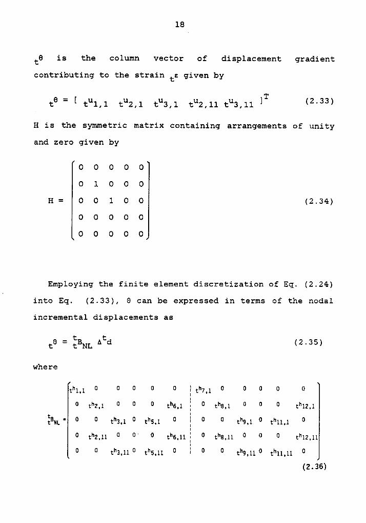
tü is the column vector of displacement gradient
contributing to the strain ts given by
0 = [ u u u u u 1T(2 33)t t 1,1 t 2,1 t 3,1 t 2,11 t 3,11 '
H is the symmetric matrix containing arrangements of unity
and zero given by
O 0 O O O
O 1 O O O
H = O O 1 O O (2.34)
O O O O 0
O O O O O
Employing the finite element discretization of Eq. (2.24)
into Eq. (2.33), 0 can be expressed in terms of the nodal
incremental displacements as
_ t tt0 —tBNL A d (2.35)
where
thll 0 0 0 0 0 }th71 0 0 0 O 09
I SI
°:*2,1 ° ° ° :*6,1 I °
:*6,1 ° ° °:*12,1
I
@11;* ** ** :*2,1 ** :*6,1 ** I ** ** :*9,1 ** :*11,1 **I
°:*2,11 °
°'° :*6,11 I ° :*6,11 ° ° °
:*12,11
** ** :*2,11** :**6,11 ** I ** ** :*9,11** :*11,11 **(2.36)
19 -
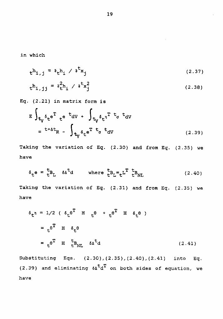
in which
h = a h /atx
(2 37)t i,j t i j '
_ 2 t 2thiljj - athi / a xj (2.38)
Eq. (2.21) in matrix form is
E StV6teT te tdv + Lvatnfr to tdV
= t*^tR - StvÖt€Ttc tdv (2.39)
Taking the Variation of Eq. (2.30) and from Eq. (2.35) we
have
_ t t t _ T töte - tBL 6A d where tBL—tL tBNL (2.40)
Taking the Variation of Eq. (2.31) and from Eq. (2.35) we
have
_ T Tötn — 1/2 ( öt0 H tü + tö H ötü )
_ T- ta H ata
_ T t t— t0 H tBNL 6A d (2.41)
Substituting Eqs. (2.30),(2.35),(2.40),(2.41) into Eq.
(2.39) and eliminating öAtdT on both sides of equation, we
have

2O
tT 1:T 1: t 1: T1: 1: 1: 1:3-tVtBL E tBL A d dV +-LvtBNL 6 H tBNL A d dV
= t+^tr - t6 tdV (2.42)tVtL1:+At . .Where r 1S the vector of externally applied element no-
dal loads at time t+At in the local coordinate system.
Let
0 0 0 0 0
0 t6 0 0 0”°1=t6H=0 OtOOO (2.43)
O O O 0 O
0 0 0 0 0
which is a symmetric Cauchy stress matrix in configuration
at time t.
Substituting Eq. (2.43) into Eq. (2.42) we obtain the incre-
mental equilibrium equation
(2.44)
where
1: _ :*2 1: 1:tkL —StVtBLEtBL dV (2.45)
1: _ 1: Tt 1: 1:tkm]-StVtBNL 1 tBNL dV (2.46)
u k _ c+At k _ c+At k—1A d — td td (2_47)
21
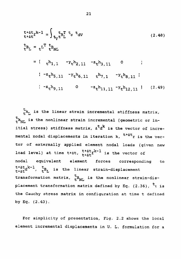
t+At k-1 _S t T t t
t+Atf—
tVtBL 0 dV (2.48)
t _ T tcBL ' t2 tBNL
= ( th1,l -yth2,l1 _zth3,1l O )
( -zth5,l1 -yth6,11 th7,l —yth8,ll (
· - - -· Zth9,ll O zthll,l1 ythl2,l1 ) (2*49)
EkL is the linear strain incremental stiffness matrix,t is the nonlinear strain incremental (geometric or in-t L
itial stress) stiffness matrix, Atdk is the vector of incre-
mental nodal displacements in iteration k, t+Atr is the vec-
tor of externally applied element nodal loads (given new
load level) at time t+At, Eiääfk-1 is the vector ofnodal equivalent element forces corresponding to
EIä€dk—1, EBL is the linear strain-displacement
transformation matrix, EBNL is the nonlinear strain-dis-placement transformation matrix defined by Eq. (2.36), tr is
the Cauchy stress matrix in configuration at time t defined
by Eq. (2.43).
For simplicity of presentation, Fig. 2.2 shows the local
element incremental displacements in U. L. formulation for a

22
6 1;+A xl6+46}: 6+46C
2 .Ätd6 3 61 td l:2 ^ 6 ^ 5
*61; *14 612 4 d4
4 dl
O *¤*2
O
:2 °c
Lxl
Fig. 2.2 Local Element Displacements in U.L.
Formulation for Plane Frame
23
plane frame, although the theoretical development is carried
out for a space frame.
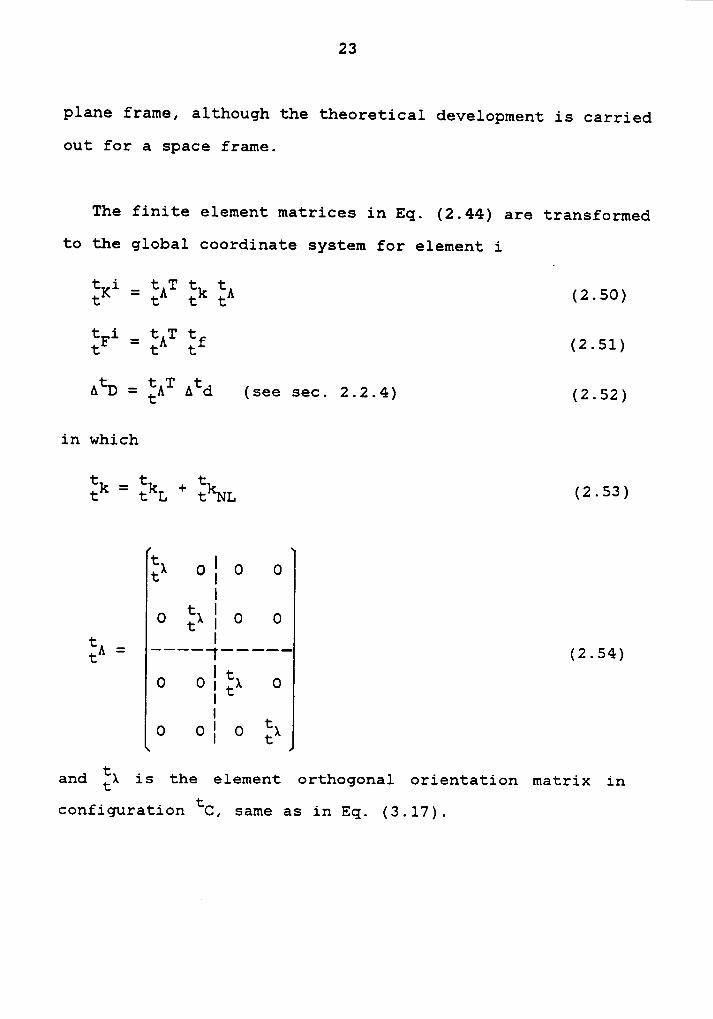
The finite element matrices in Eq. (2.44) are transformed
to the global coordinate system for element i
t i _ t T t ttK — tA tk tA (2.50)
t i _ t T ttF — tA tf (2.51)
AtD = EAT Atd (See sec. 2.2.4) (2.52)
in which
t _ t tuk “ ckn. + +;k1~1L (2.53)
t Itl O I O 0
I1:0 tx I 0 0tA — ———— I ————— 2 54t — ·I I - >
0 0I;) 0I
I t0 O I 0 tx
and Ex is the element orthogonal orientation matrix in
configuration tC, same as in Eq. (3.17).

24
By employing the member code technique [28] (i.e. direct
stiffness procedure), the incremental equilibrium equation
in U.L. formulation of the whole structure is
EK Aqk = t+^tQ - EIQEFRÄ (2.55)
where
EK = structural strain incremental stiffness matrix
corresponding to qk-1
Aqk= vector of incremental nodal displacements at kth
iteration in configuration at time t
t+AtQ= vector of given new load level in configuration
configuration at time t+At
§I2EFk—l = vector of nodal equivalent element
forces corresponding to qk_1
qk_l= vector of nodal displacements at k—l iteration
Here the structural tangent stiffness matrix K, is a
function of displacements q, since the problem is nonlinear.
In Eq. (2.55) the response of a nonlinear structure may be
approximated for incremental nodal displacements by a linear
relationship. Because the final configuration is based on
equilibrium balance between the nodal element forces and the
applied nodal load, the stiffness used to solve Eq. (2.55)
need not be exact [41].
25
2.2.4 Transformation Matrix
The global element displacements are transformed to the
local element displacements by the transformation (Fig. 2.2
to Fig. 2.4)
t _ t ttd — tA tD (2.56)
Similarly, the local element forces are transformed to
the global element forces by equation
t i _ t T ttF — tA tf (2.57)
where EA is transformation matrix defined by Eq. (2.54).
Because all variables refer to the current deformed con-
figuration tcin the U.L. formulation, the transformation
matrix §A in Eq. (2.54) remains constant from configura-
tion tc to t+AtC. Eqs. (2.56) and (2.57) yield the incre-
ments of local element displacements and global element
forces
Atd = EA AtD (2.58)
AtFi = IQAT Atf (2.59)
26
*2 fll’d1l ll xlfd6*6
flO’dlOfsrds2*
2\ fl2’d12
z. :11* 1
z ,.1E X3
X2
/ X1X6
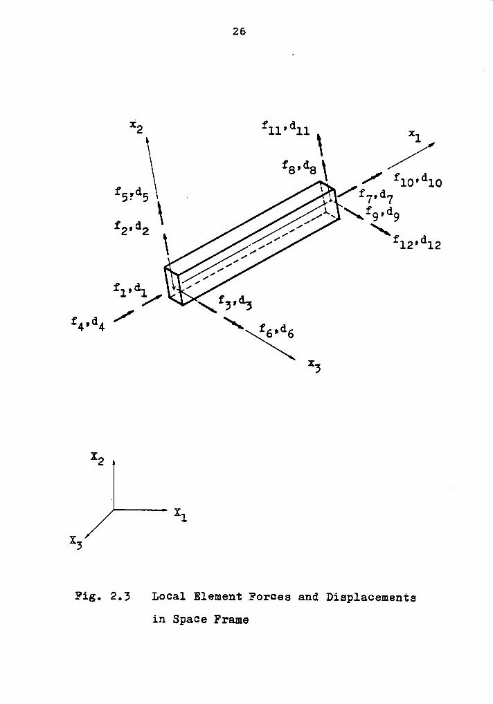
Fig. 2.3 Local Element Forces and Displacements
in Space Frame
zv
Fll’Dll
Fa•Da
1/Fl2’Dl2
F5•Ds . /F9'D9 „—•· —•-F D10- lO
x2 0
LX1 .X3
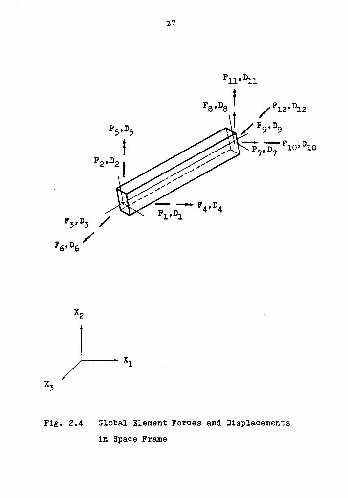
Fig. 2.4 Global Element Forces and Displacements
in Space Frame
28
where Atf and AtFi are the vectors of the local and global
incremental element forces from time t to t+At respectively,
referred to configuration at time t.
2.3 INCREMENTAL EQUILIBRIUM EQUATION lg T.Q. FORMULATION
2.3.1 Incremental T.g. Continuum Mechanics Formulation
The T.L. formulation is based on the same procedures that
are used in the U.L. formulation, but all variables refer to
the initial undeformed configuration Oc at time O (Fig.
2.1).
Taking the Variation of Eq. (2.8), we have
t+At _6 Osij
— öosij (2.60)
Substituting Eqs. (2.7), (2.60) into Eq. (2.2)
t O 0 _ t+At*5Ov, Osij öosij dV + OV 0Sij öosij dV - R (2.61)
The strain increment components can be separated into linear
and nonlinear parts
0%; = 0%; + 0%; (2*62)
where
e = 1/2 ( u + u + tu uO ij O i,j O j,i O k,i O k,jt+ Oukli Ouklj) (2.63)
29
Onij = 1/2 Ouk i Ouk j (2.64)
_ OOuilj — 8 ui / 8 xj (2.65)
1: _ 1: 0 'ouilj — 8 ui / 8 xj (Z-66)
Onij lS the nonlinear part of strain increment Osij, Oui jis the derivative of displacement increment with respect to
local coordinate Oxj, äui j is the derivative of dislace-ment component in configuration at time t with respect to
local coordinate Oxj.
The constitutive law is [10]
0S1j = ocijrs 0°rs (2·67)
where OCijrS is the component of incremental material prop-
erty tensor at time 0 referred to the configuration at time
O.
Using Eqs. (2.62), (2.67), Eq. (2.61) can be transformed to
O S_t O,[oV ocijrs 0*:s d0°15 dv 0V osij d0“1j dv
_ t+At _ t O- R gov Osij aoeij dV (2-68)
Eq. (2.68) is nonlinear in the incremental displacements ui,
and it can be linearized by using the approximations
öosij = öoeij (2.69)
30
osij = ocijz-5OersThen
Eq. (2.68) becomes
O S t Ogov Ocijrs Oers do%3 dv + ov 0%; 60**13 dv_ t+At _ t Ü 2R Lv Osij soeij dV ( - )
which is linear equation in the incremental displacements
ui, corresponding to the local coordinate system.
For three dimensional beam element with small deformation
and uniaxial state of strain (i.e.0:11 only), in which tor-
sion is treated independently, Eq. (2.71) can be specialized
as
·d
O t 0E Sg Oell öoell dV +jg. Oc öonll dVV} V
_ t+A‘C _ t O 2_72- R so 05 öoell dV ( )V
where
t _ tog - 0511 (2.73)is the 2nd Piola—Kirchhoff stress.
31
2.3.2 Incremental Strain
The incremental displacement components along the cen-
troid axis of elements are interpolated as
0¤d1
Aodz
001 001 0 0 0 0 01
OÜ7 0 0 0 0 0 .I002 - 0 002 0 0 0 000E
0 000 0 0 0 0012 . (2.174)
_ 0¤d11
^°°12
where
Oui = increment in displacement component of element from
t to t+At measured in the local axes Oxi; i=l,2,3
Ohk = finite element interpolation function corresponding
to Aodk, k = 1 to 12
Aodk= increment in nodal displacement component of
element from t to t+At measures in the localOaxes xi
Neglecting the 2nd order terms of äulll, Oulil, from Eq.(2.62) the incremental uniaxial strain along the beam ele-
ment for small deformation is
Osll = Oell + Onll ° (2*75)
32
where
e = u + tu u + tu u0 11 0 1,1 0 2,1 O 2,1 O 3,1 0 3,1¤-—v——v \-•——————1g,————•—————1
due to due to initialaxial force displacement
;l’.<>3a11j,f.¤B=111due to bending (2.76)
n = 1/2 ( u )2+ 1/2 ( u )2
(2 77)0 11 O 2,1 O 3,1 ‘
and
äui j = atui/
6Oxjj (2.78)
2.3.3 Incremental Eguilibrium Eggation
Expressing Eqs. (2.75), (2.76), (2.77) in matrix form in-
troduced by Wood and Schrefler [6]
Os = Oe + On (2.80)
where
Oe = OLT 00 (2.81)_ TOn — 1/2 00 H 00 (2.82)
33
T _ t tOL - [ 1 Ouzll Ou3I1 y z ] (2.83)
_T00 “
* 0**1,1 0**2,1 0**6,1 0**2,11 0**6,11**2·0‘**
OLT is the row vector defining linear strains Oe fromdisplacement gradients, 00 is the column vector of displace-
ment gradient contributing to the strain Os, H is defined as
in Eq. (2.34).
Employing Eq. (2.74) into Eq. (2.84), we express 0 in
terms of the nodal incremental displacements as
_ t OOG — OBNL A d (2.85)
where _
0n1_1 0 0 0 0 0 { 0h7’1 0 0 0 0 01 ,
° 0**2,1 ** ° °0**6,1*
°0**6,1
° ** ** 0**12,1I
*5 ' ** ** 0**6,1 **0**6,1° * ** ** 0**9,1 **0**11,1 **0uL {
** 0**2,11 ** ° °0**6,11*
° 0**6,11° ** ° 0**12,11
I
° ** 0**6,11°0**s,11 ** * ° ** 0**6,11**0**11,11°(2.86)
in which
_ OObi j - aohi / 6 xj (2.87)
34
- 2 O 2 2.88Ohiljj -aohi/axj (( )
Eq. (2.72) in matrix form is
E ¤° °°" * IW ‘¤"T §° §¤ ¤dv (2.89)
Taking the Variation of Eq. (2.81) and using Eq. (2.85) we
obtain •
öoe = EBL 6AOd (2.90)
where
t _ T t _ t t0BL. ‘ 0L 0Bm. ‘ 0BLo ‘“OBL1 (2·91a)
and
tI¤°L¤ ° [¤“1•1
"¤"2.l1 " ¤"3.11
°·¢ 0h5,11 ·¥ oh6,11 ;
E ¤h7,1 ·Y ¤h8,l1 ·* ¤h9,l1° -= „¤11,11 -y ,,h12_11] (2_Q1b)
c z c z ,¤BL1‘ L~° ¤“2.1 ¤*‘2.1 ¤u3„1¤h3,1 °¤u3,1 o"s.1 §u2,1oh6,1 :
{ t c c c· ° ¤u2,1 0h8,1 ou3,l oh9,1 ° 0u3,1 ¤"11,1 ou2,1 0*112,1] (2·9l°)
Taking the Variation of Eq. (2.82) and from Eq. (2.85) we
have
35
1 T T6°n 2 (606 H O6 + oa H 606)T= 06 H 6°6
T t= 6 H B 6A°d0 0 NL (2.92)
Substituting Eqs. (2.81),(2.85),(2.90),(2.92) into Eq.
(2.89), we have
I,v ÄBI E ÄBL 6¤d odv + [0V §6;L S6 H :B„L ¤°d °dV ;° °dV ·
. (2.93)
Let
I0 0 0 0 0
0 Qu 0 0 0gs- gun - 0 0 gc 0 0 (2.94)
_ 0 0 0 0 0
0 0 0 0 0
which is the 2nd Piola-Kirchhoff stress matrix.
Substituting Eq. (2.94) into Eq. (2.93), we obtain the in-
cremental equilibrium equation
(ERL + äkNL) AOdk = t+Atr _ t+Aäfk—l (2.95)
where1
36
t _ t T t O .0kL — OVOBL E OBL dV (2.96)T
0kNL =_)· tB T ts tB Odv 2 97)ovo NL. 0 0 NL. ( ·Aodk = vector of incremental nodal displacement at
time t in iteraion k; i.e.
t+Aädk = t+Aädk-1 + A0dk (2.98)t+At _ .r — vector of externally applied element nodal
loads at time t+Att+At k·1 _ t T t 0Of —
SOVOBL Oc dV (2.99)
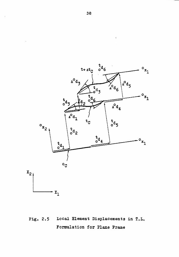
For the simplicity of presentation, Fig. 2.5 shows the
local element displacements in T.L. formulation for a plane
frame.
The finite element matrices in Eq. (2.95) are transformed
to the global coordinate system for element i
t i _ t T t tOK — OA Ok OA .· (2.100)
t i _ t T tOF — OA Of (2.101)
AOD = äAT Aoca (see sec. 2.3.4) (2.102)
in which
t = t t 103)ok 0kL ‘”0kNL (z'
37
äA = transformation matrix (see sec. 2.3.4)
Employing the member code technique [28], the incremental
equilibrium equation in T.L. formulation of the whole struc-
ture is
3K Aqk = t+AtQ _ t+AäE.k-1 (ZJO4)
2.3.4 Transformation Matrix
Similar to Eqs. (2.56) to (2.59), we have (Fig. 2.3 to
Fig. 2.5)
t _ t t _Od - OA OD (2.105)
t __ t TtOF- OA Of (2. )
where
tO). 0 0 0
t 0 E1 0 00 A = t (2.107)0 0 >. 00
t0 0 0 Ox
38
t ,t+ Atc .od6 oxl
oA dsO A°d5
tdAo5— td OX1
O 3 :2 Aqd. 4
oA dl tc tao o 5x2 td
o 2td o
td ·/·"'
°cX2\
X1
Fig. 2.5 Local Element Displacements in T.L.
Formulation for Plane Frame
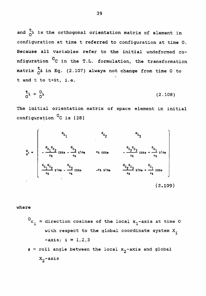
39
and gl is the orthogonal orientation matrix of element in
configuration at time t referred to configuration at time 0.
Because all variables refer to the initial undeformed co-
nfiguration Ocin the T.L. formulation, the transformation
matrix SA in Eq. (2.107) always not change from time 0 to
t and t to t+At, i.e.·
t _ 0Ok — OA (2.108)
The initial orientation matrix of space element in initial
configurationOc
is [28]
ocl 6cz 6c3
6 6 6 66glcom sim ¤1 c6s• -
ig- c6s« + —l sim¤1 ¤1 ¤1 ¤1
6 6 6 6 6 6sim cos¢ -91. sim li sim cos6
0; I 0; 0; 0;
(2.109)
where
Oci = direction cosines of the local x1—axis at time 0
with respect to the global coordinate system Xi
—axis; i = 1,2,3
¢ = roll angle between the local x2—axis and global
X2-axis

40
Oz = (Oc? + °c§)l/2 (2.110)
Eqs. (2.105), (2.106) yield the increments of the local
element displacements and global element forces in T.L. for-
mulation
Aod = gA 100 (2.111)
AOFi=
gAT Aof(2.112)
where Aof and AOFi are the vectors of the lcoal and global
incremental element forces from time t to t+At respectively,
referred to configuration at time 0.
2.4 CONVECTED COORDINATE FORMULATION
In the convected coordiante formulation developed by Be-
lytschko [5], [17], all variables refer to the new incre-
mented configuration at time t+At. The convected coordinate
system means that each element is associated with a rigid
cartesian coordinate system that rotates and translates with
the element but does not deform with the element. Because
the coordinate systems corresponding to the configurations
at time t and t+At are independent of each other, an incre-
mented concept in this formulation cannot be directly ap-
plied [18]. Hence, in the convected coordinate formulation
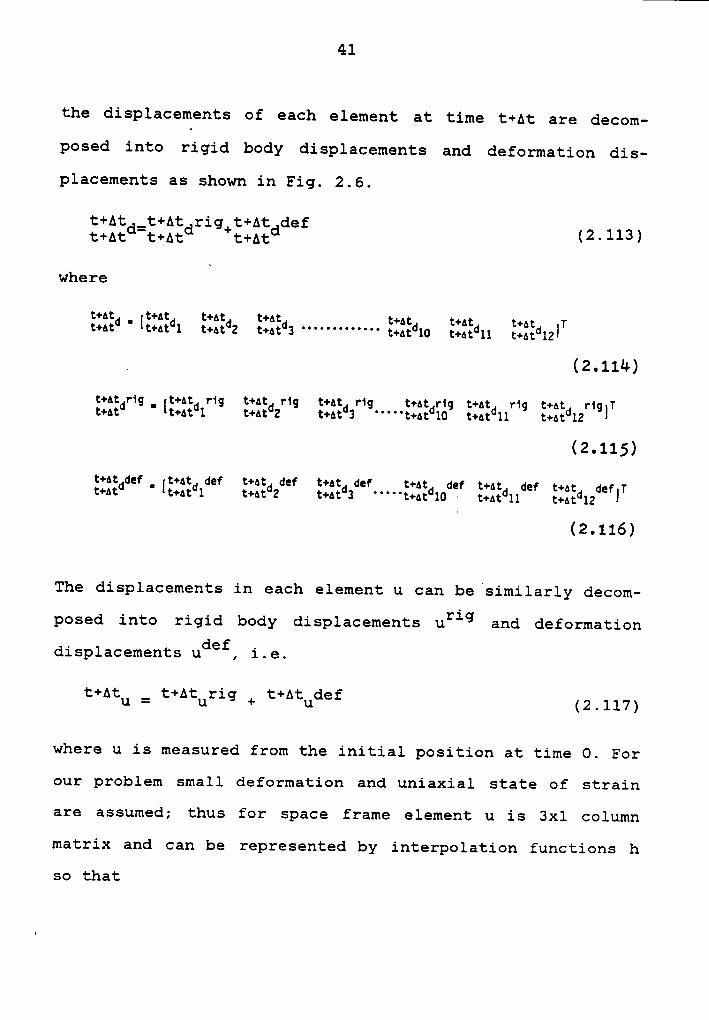
41
the displacements of each element at time t+At are decom-
posed into rigid body displacements and deformation dis-
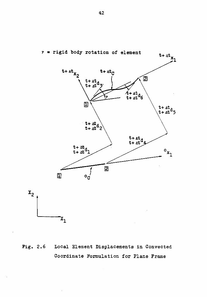
placements as shown in Fig. 2.6.
t+At _t+At rig t+At deft+Atd-t+Atd +t+Atd (2.113)
where
:+4: _ :+4: :+4: :+4: : : : ::+4:d [:+4:dl :+4:d2 :+4:d3 '°'''°'''‘''' ::::d10 tiätdll:::€d;z]T
_ (2.114)
:+4:dr1g_
[:+4:d rig :+4:d rig :+4:d rig :+4:dr1g :+4:d rig :+4:d r1g]T:+4: :+4: 1 :+4: 2 :+4: 3 ''''':+4: 10 :+4: 11 :+4: 12
(2.115)
:+4: def. :+4: def :+4: def :+4: df :4: df t : dfÜütd[C+Atd]. t+AtdZ t+4td3
e""'tißtdlo tzgtdll(2.116)
The displacements in each element u can be similarly decom-
1>¤S¤d i¤t<> riqid b¤dy displacements urig and deformationdisplacements udef,
i.e.
t+Atu = t+Aturig + t+Atudef (2*117)
where u is measured from the initial position at time O. For
our problem small deformation and uniaxial state of strain
are assumed; thus for space frame element u is 3xl column
matrix and can be represented by interpolation functions h
so that
42
v = rigid body rotation of element 1:+ Atxl
t+ Atxz t+AtcI2]t+ Atd
t+ At+At -v t+ nds
1 1:+ Atdt+At 5
1:+ Atdt+ At 2
t+Att+ Atd
t+ At L
E °g
X2 ‘
X1 .
Fig. 2.6 Local Element Displacements in Convected
Coordinate Formulation for Plane Frame
43
:0:tiatdl
mädzt‘^tu1hl 0 0 0 0 0 E hy 0 0 0 0
0AE
"*^*u2-0 nzo 0 0 hs E 0 nac 0 0 nlz•E°*^°03 0 0 ng 0 n5‘ 0 { 0 0 ng 0 nll 0 g
t ctiätdll1:+Atd1:+6: 12
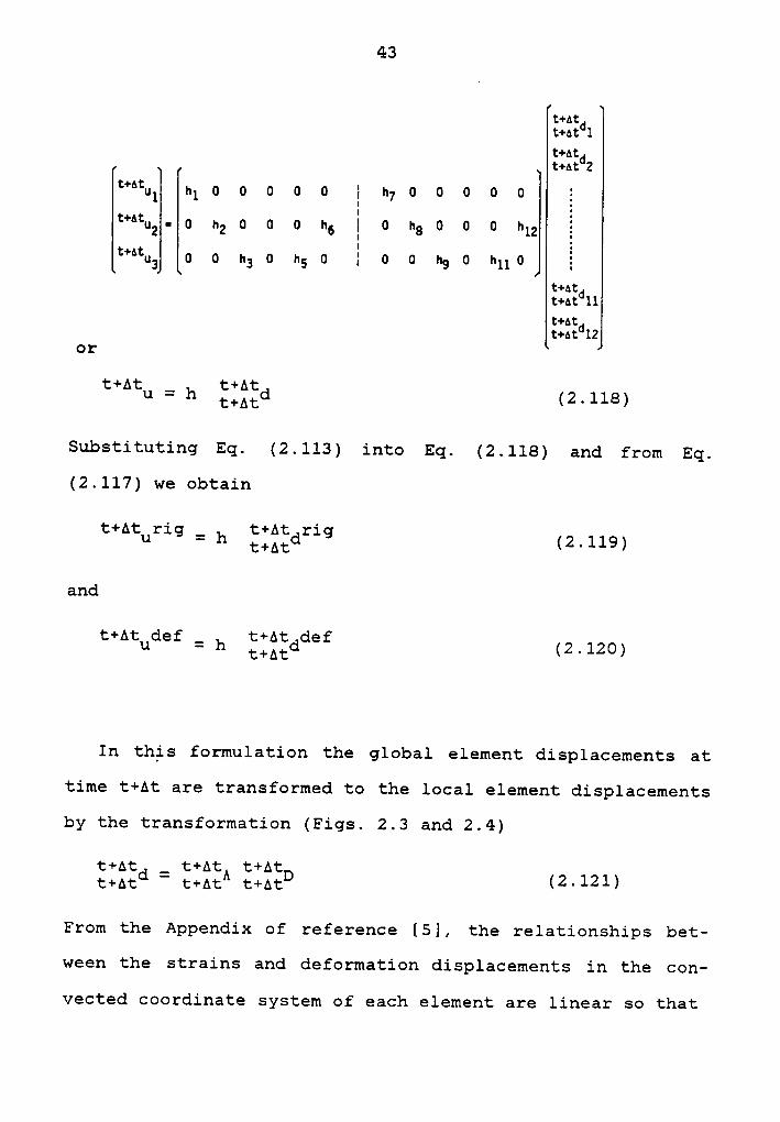
or
t+At _ t+Atu — h t+Atd (2.118)
Substituting Eq. (2.113) into Eq. (2.118) and from Eq.
(2.117) we obtain
t+At rig _ t+At rigu — h t+Atd (2.119)
and
t+At def _ t+At defu — h t+Atd (2.120)
In this formulation the global element displacements at
time t+At are transformed to the local element displacements
by the transformation (Figs. 2.3 and 2.4)
t+At _ t+At t+Att+A1;d ' 1;+A·c^ 1;+AtD (2-121)
From the Appendix of reference [5], the relationships bet-
ween the strains and deformation displacements in the con-
vected coordinate system of each element are linear so that
44
t+At _ t+At déf 2BL t+A1;d ' ( )
where BL is the linear strain displacement transformation
matrix and can be obtained from the Eq. (2.120) and appro-
priate linear strain displacement equations.
As shown in the appendix of reference [5], consider two
successive configurations at time t and t+At,tho global in-
ternal nodal forces of each element can be derived from the
principle of Virtual work and it yields
t+At =t+At T t+At t+At . (2_l23BL O dv )
Vt _ t T T t t .tF — tA §¥VBL c dV (2.124)
. . t t+At . .in which o and c are the axial Cauchy stresses at time
t and t+At respectively, V is the element volume which the
change of volume can be neglected in the volume integration
for small deformations, A is the transformation matrix from
the global coordinate system to the convected, coordinate
system, defining
t _ t+At _ tA A —t+AtA tA (2.125)
Atc=
t+Atc — to(2.126)
and
45
t _ t+At _ tA F —t+AtF tF (2.127)
From Eqs. (2.123) to (2.127), we obtain
A°°B‘=tAT BT Ata dV+AtAT BT t+^t¤ dV · 1 (2-128)t V L V L
To establish the global tangent stiffness matrix for an
element, we must express Ata and AtA in Eq. (2.128) in terms
of the nodal incremental displacements AtD defined as
_ t+A _AtD - UAED ED (2.129)
Because in this convected coordinate system the nodal
element dsiplacements between the configurations at time t
and t+At are independent of each other, the nodal incremen-
E tal displacements in Eq. (2.129) are not vector quantity.
Hence, it is inappropriate to express Ata and AtA in Eq.
(2.128) in terms of AtD.Therefore, using the finite ele-
ment model in the convected coordinate formulation to estab-
lish the local element tangent stiffness matrix is inconve—
nient.
46
2.5 COMPARISON gg Q.L. AND T.L. FORMULATIONS
The main difference between the U.L. and T.L. formula-
tions lies in the coordinate system referred to formulate
the incremental equilibrium equations; the former refers to
the current deformed configuration tC; the latter refers to
the initial undeformed configuration OC.
Regardless of which formulation used, we will show that
the incremental equilibrium Eqs. (2.55) and (2.104) are
identical in both formulations [9]. From Eqs. (2.50) and
(2.100) the global element tangent stiffness matrices are
t i _ t T t ttK — tA tk tA
for U.L. formulation (2.130)
Elf = Ef El Elfor T.L. formulation (2.131)
in which
EA, SA = transformation matrix between the local
coordinate axes in configuration at time t and
the global coordinate axes
Let
t _ ttA — R OA (2.132)
47
where R is the transformation matrix from the local coordi-
nates Oxi to txi in space (Fig. 2.1); it has been derived by
Bathe [9] and will not be described here.
Substituting Eq. (2.132) into (2.130)
t i _ t T t ttK — OA Ok OA (2.133)
where
t _ T tOk — R tk R (2.134)
From Eqs. (2.131) and (2.133), we have
t i _ t itK — OK (2.135)
Therefore, the global element tangent stiffness matrices
Ki are identical in both formulations.
As a result of Eq. (2.135), the assembled system tangent
stiffness matrices K in Eqs. (2.55) and (2.104) are identi-
cal in both formulations.
t _ ttK — OK (2.136)
Similarly, from Eqs. (2.51),(2.101) the global element forc-
es are
+;+A1;F1k'l = t+At^k-1T t+Atfk-1t+At t+At t+At
48
for U.L. formulation (2.137)
t+AtE.ik-1 = t+At^k—1T t+Atfk—1O O O
for T.L. formulation (2.138)
Substituting Eq. (2.132) into Eq. (2.137)
.k-1 Tt+At 1 _ t+At k-1 t+At k-1t+AtF
— OA Of (2.139)
where
t+^§fk‘T = RT äääfkd (2.140)
From Eqs. (2.138),(2.139), we have
.k-1 .k—1t+At 1 _ t+At 1t+AtF
— OF (2.141)
Therefore, the global element force vectors are identical
in both formulations.
As a result of Eq. (2.141), the vectors of equivalent no-
dal element forces F in Eqs. (2.55),(2.104) are identical in
both formulations.
t+At k-1 _ t+At k-1t+AtF
— OF (2.142)
49
From Eqs. (2.136),(2.l42) we may conclude that the incre-
mental equilibrium Eqs. (2.55) and (2.104) are identical in
both formulations.
As a result of Eqs. (2.55) and (2.104), we are led to the
conclusion that
The main advantages of the U.L. formulation are:
l. Since the rotation referred to the current configura-
tion tc is infinitesimal, it can be treated as vector
in space frame [2], [18].
2. The linear incremental strains in Eq. (2.12), refer-
red to the current configurationtC,
not include the
initial displacement effect; it results that the li-
near strain incremental stiffness matrix EKL in Eq.
(2.55) is not including the initial displacement ef-
fect.
3. Because the strains, referred to the current configu-
ration tC, are so infinitesimal that sometimes we can
neglect the nonlinear part of incremental strains in
Eq. (2.11); it results that even the nonlinear strain
incremental stiffness matrix EKNL in Eq. (2.55) can
be omited. In fact, as we pointed out earlier, the
stiffness used to solve Eq. (2.55) need not be exact.

50
4. Items 2 and 3 result that simple and approximate for-
mulations of the U.L. in Eq. (2.55) may be developed,
which make the U.L. formulation very efficient and
clearly superior to the T.L. formulation.
5. Especially more suitable for the large displacement
but small strain problems which are very common in
practice for many types of problems [36].
6. If the relative member deformations are small enough
that. we can. directly employ the beam-column. model
which uses convected coordinate system to formulate
the tangent stiffness matrix and nodal equivalent
force in Eq. (2.55), in addition to finite element
model.
The disadvantages of the U.L. formulation are:
l. The transformation matrix EA in Eq. (2.54), refer-
red to the current configuration tC, must be updated
at each time step (iteration).
2. The stresses at time t+At as in Eq. (2.5)
Umésij = t‘1j + tsij
where the stress increments tSij from time t to t+At
are the 2nd Piola—Kirchhoff stresses referred to time
t, which must be transformed into Cauchy stresses.
51 „
_Therefore, it is slightly more complicated than. in
T.L. formulation to compute the stresses [36].
3. Mass matrix would be updated at each iteration which
leads to complexity in the U.L. formulation to dynam-
ic problems.
4. As to economic consideration, items l to 3 result in
more computational effort than T.L. formulation.
On the other hand, the advantages of the T.L. formulation
are:
1. The transformation matrix SA in Eq. (2.107) remains
unchanged throughout each iteration as in Eq.
(2.108).
2. The use of a unique type of the 2nd Piola—Kirchhoff
stresses in Eq. (2.7).
3. Because the mass matrix would then be constant in the
extension to dynamic problems throughout each itera-
tion, it leads to simplification in the T.L. formula-
tion [12], [3].
4. Items 1 to 3 result in less computional effort than
U.L. formulation which saves computer time and money.
The disadvantages of the T.L. formulation are:
52
1. Because the rotation referred to the undeformed con-
figurationOc
is finite, it cannot be treated as vec-
tor in space problems; therefore, the merit of matrix
operation will be lost [3], [18].
2. The linear incremental strains in Eq. (2.63), refer-
red to the initial configuration OC,include the ini-
tial displacement effect; it results that the linear
strain incremental stiffness matrix EKL in Eq.
(2.104) include the initial displacement effect.
3. Because the strains referred to the initial configu-
ration Oc is finite, as displacements become larger
and larger, nonlinear term of incremental strains in
Eq. (2.62) are significant; in other words, the non-
linear strain incremental stiffness matrix SKNL in
Eq. (2.104) must be taken into account to obtain the
exact stiffness for large displacements.
4. Employing the beam-column model, which uses convected
coordinate system, in T.L. formulation, the local
element stiffness matrix and force vector must. be
transformed to the initial coordinate system.
In conclusion, no matter which formulation we use, the
same structural stiffness matrices and nodal equivalent ele-
53
ment forces should be obtained. Therefore, the solutions
using different formulations must be the same, if the same
number of elements are employed [9]. whether to use the
U.L. or the T.L. formulations depends largely on the program
design and the practical problems. In beam analysis the U.L.
formulation is more effective than the T.L. formulation in
which the additional ÄBL1 matrix must be evaluated as in
Eq. (2.91c). Based on this concept, in next chapters we will
only employ the U.L. formualtion to solve the incremental
equilibrium equation as shown in Eq. (2.55).
Chapter III
DEFORMATION DISPLACEMENTS OF SPACE FRAME ELEMENT
3.1 INTRODUCTION
The element displacements are decomposed into rigid body
displacements and deformation dispacements. In this chapter
the deformation displacements are derived for a space frame
element with large displacements and rotations of nodes and
members. However, the strain in each element is assumed to
be small; that is, the element deformations are restricted
to be small. Four types of coordinate systems are employed
to derive the element deformation displacements.
The beam element is assumed to be straight and so slender
that shear deformations can be neglected in comparison with
bending deformations. It is assumed that the cross section
of the beam remains plane and normal to the centroidal axis
during deformation. The cross section is doubly symmetric,
and the torsional stiffness will be treated independently
from bending and axial stiffnesses. However, interaction of
axial force and bending is considered [21].I
54
55
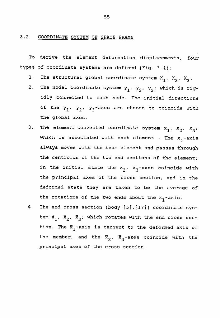
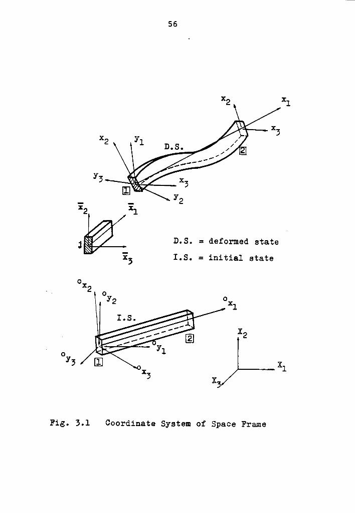
3.2 COORDINATE SYSTEM QF SQQQE FQQME
To derive the element deformation displacements, four
types of coordinate systems are defined (Fig. 3.1):
1. The structural global coordinate system X1, X2, X3.2. The nodal coordinate system yl, y2, y3; which is rig-
idly connected to each node. The initial directions
of the yl, y2, y3—axes are chosen to coincide with
the global axes.
3. The element convected coordinate system xl, x2, x3;which is associated with each element . The x1—axisalways moves with the beam element and passes through
the centroids of the two end sections of the element;
in the initial state the x2, x3-axes coincide withthe principal axes of the cross section, and in the
deformed state they are taken to be the average of
the rotations of the two ends about the xl-axis.4. The end cross section (body [5],[l7]) coordinate sys-
tem xl, x2, E3; which rotates with the end cross sec-
tion. The xl—axis is tangent to the deformed axis of
the member, and the R2, E3-axes coincide with theprincipal axes of the cross section.
56
x2 xl
)\‘xl
X Y2 J- D•S• l
Y; Ql ol?
-_ y2
*2 *1
D.S. = deformed stateE3 I.S. = initial state
o._ *2 Oy O2 l xl
X2O s yl
V3 l _ - xlx3 x3
Fig. 3.1 Coordinate System of Space Frame
57
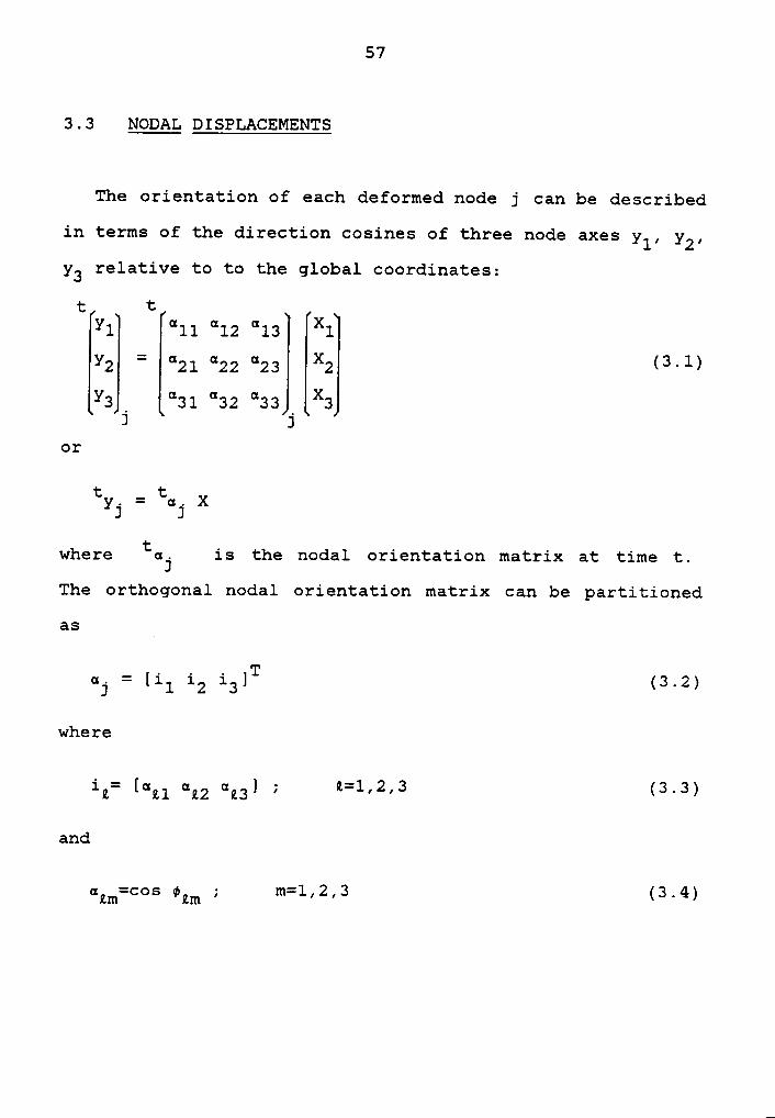
3.3 NODAL DISPLACEMENTS
The orientation of each deformed node j can be described
in terms of the direction cosines of three node axes yl, y2,
y3 relative to to the global coordinates:
t tY1 all °‘12 °l3 X1y2 = ¤2l ¤22 °‘22 X2 (31)Ya _ (131 ¤32 °‘2„:s _ X2
J Jor
t t. = . XY1 GJ
where taj is the nodal orientation matrix at time t.The orthogonal nodal orientation matrix can be partitioned
as _
aj = [il 12 i3]T(3.2)
where
iß= [all aßzaßß] ; ß=l,2,3 (3.3)
and
a£m=cos ¢£m ; m=l,2,3 (3.4)

58
atm is the direction cosine and ¢ßm is the direction an-gle between the nodal yß-axis and the global Xm—axis.
In analyzing large displacements of a space frame, the
deformed configuration of each node j can be represented in
terms of a translation vector [Djl DjzDj3]T relative to the
global coordinate system and an node orientation matrix aj.
Consider the increments of nodal displacements which are
assumed to be small during a load step. The incremental dis-
placement vector of node j is
AUjtAUj = ———-
(3.5)AUjr
in which AUjt, AUjr are the translational and rotationalincremental vectors of node j in the global coordinate sys-
tem:
AU = [ AD AD AD.1T
(3.6)Jt J1 J2 J3
AU. = [ AD. AD. AD. 1T(3.7)Jr J4 J5 J6
where ADjl, ADj2, ADj3 are the incremental. deflections atnode j and ADj4, ADj5, ADj6 are the incremental rotations atnode j.

59
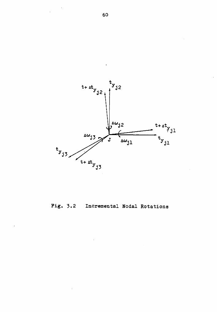
According to appendix A, the node transformation from the_configuration tc to the configuration t+AtC is (Fig. 3.2)
t+At t t. = I+ R. . 3.8Y] < J) yj ( )
where I is identity matrix and tRj is the rotation matrix atnode j, defined as
t t0 A —A .
t t tR- = - . .
'C tA w32 ·-A A31A
0
where Awji is the incremental nodal rotation at node j about
tyi—axis (Fig. 3.2), i= 1, 2, 3; defining
tA wjlt tA . = A . 3.10w] w32 ( )
tA wjß
where Atwj can be obtained from Eq. (3.1) as
t t t. = . U. 3.11A oo] aj A Jr ( )
Substituting Eq. (3.1) into Eq. (3.8) yields
t+^ty. = (I+tR.) ta. x (3.12)J J J
= ta. X + Ata. X (3.13)-3 -., --3,.-.t t. A .Y] Y]
‘60
t·¤+ At V32
AU-32 *6+ AtVjl
AU-.13 tJ Atdjl yjlt .VJ;
1:+ AtVJ3 3
Fig. 3. 2 Iucrameutal Nodal Rotatious
61
or
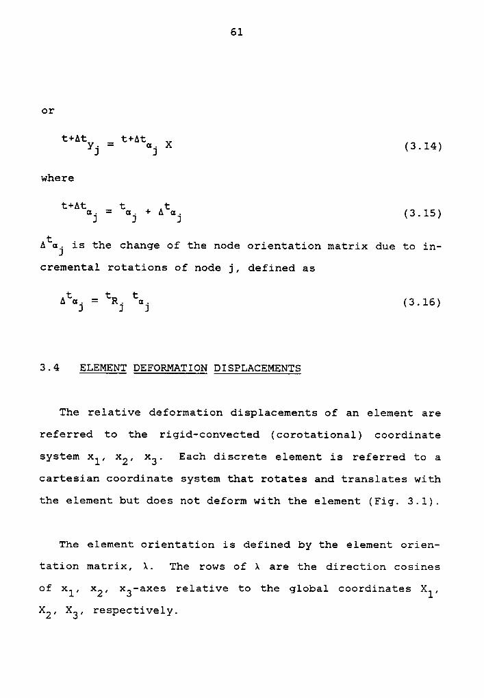
t At+y. =
t+Ata.X (3,14)J J
where
t+At t tGJ GJ aj ( ). = . + A . 3.15
Ataj is the change of the node orientation matrix due to in-
cremental rotations of node j, defined as
t t tA . = R. . 3.16°‘JJ
°”J ( )
3.4 ELEMENT DEFORMATION DISPLACEMENTS
The relative deformation displacements of an element are
referred to the rigid-convected (corotational) coordinate
system xl, x2, x3. Each discrete element is referred to acartesian coordinate system that rotates and translates with
the element but does not deform with the element (Fig. 3.1).
The element orientation is defined by the element orien-
tation matrix, X. The rows of X are the direction cosines
of xl, x2, x3-axes relative to the global coordinates X1,X2, X3, respectively.
62
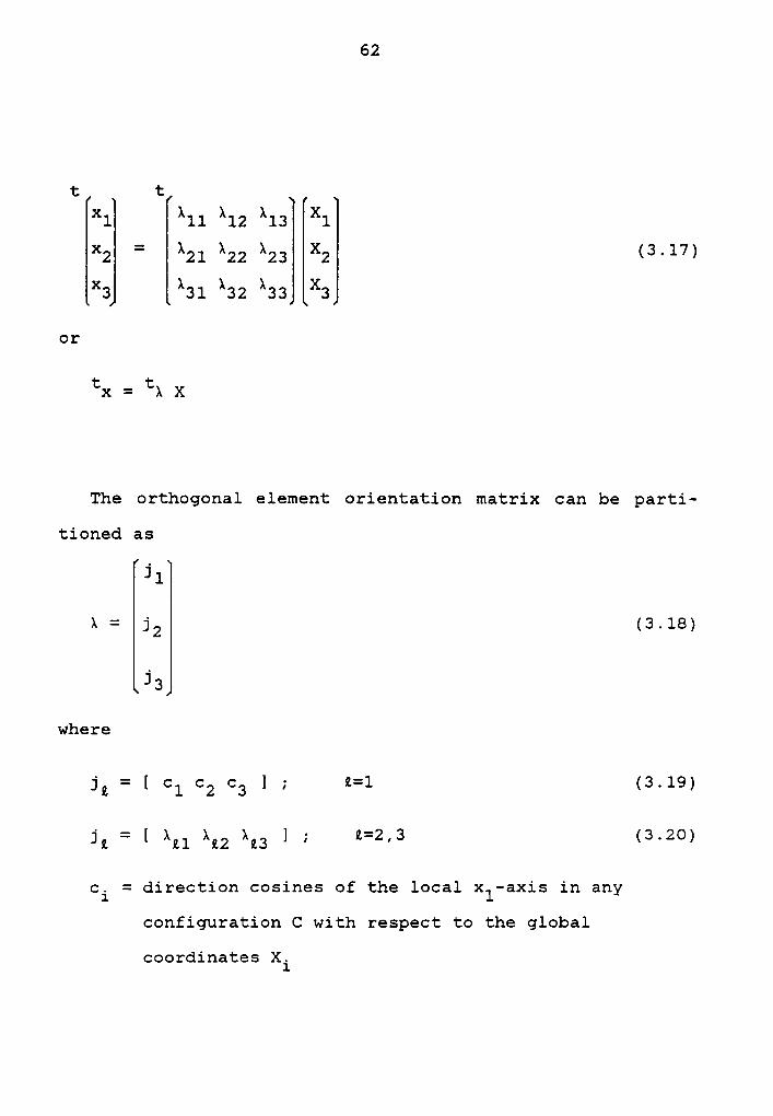
t tX1 *11 *12 *13 X1x2 = kzl XZZ X23 X2 (3.17)
X3 *31 *32 *33 X3
or
tx = tk X
The orthogonal element orientation matrix can be parti-
tioned as
jl
k = jz (3.18)
j3
where
jl = [ cl cz c3 ] ; ß=1 (3.19)
jl = [ xu xßz xu ] ; 2=2,3 (3.20)
ci = direction cosines of the local x1—axis in any
configuration C with respect to the global
coordinates Xi

63
and
Xßm = cos wßm ; m=l,2,3 (3.21)
kam is the direction consine and wßm is the direction an-
gle between the local element xß-axis and the global
X -axis.m
The element orientation matrix of a space element depends
on the orientations of the principal plane of the element
defined by the local xl, x2-axes. The initial orientation
matrix of the space element in configurationOc
is defined
in Eq. (2.109).
In the formulation developed here, no restrictions are
made on the rotations and translations of the node. However,
the relative deformations of the members are small such that
we can apply the conventional beam—column theory to the mem-
ber-force deformation relations.
The deformation displacements of a space frame element is
represented. by the end angles el3, e23, elz, e22; total °
twist ¢t, and relative axial displacemnet u (Fig. 3.3).

P64
l
- x:2 2·
\J 21M
M *5 613 P Mw'?t13
L-u uL
i'1x M
P 2 812 2 ::22 xlinn :1 1 11-·—•M12e22 P Mw'?t
E:3 3
Fig. 3.3 (Element Deformation Displacements
and Associated Forces
65
Consider the increments of nodal displacements and
element deformations which are assumed to be small during a
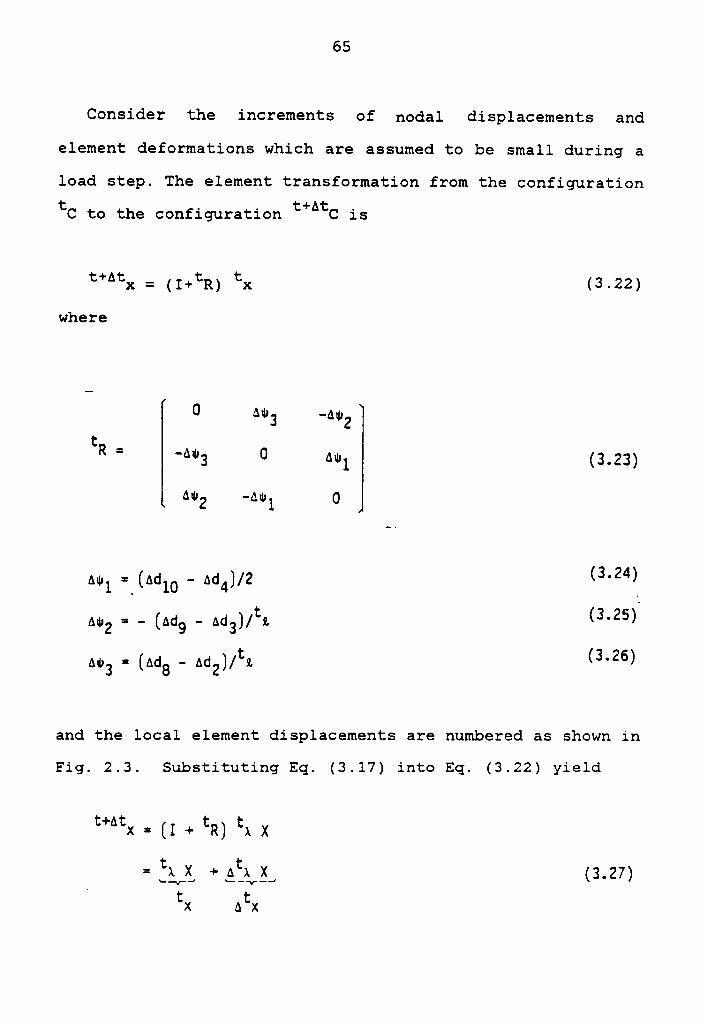
load step. The element transformation from the configurationtc to the configuration t+AtC is
t+Atx= (I+tR)
txwhere
0 -603 602tR = 6 0' W3 601 (3.23)
602 -601 O
601 = (6dlO - Ad4)/2 (3'24)
602 = —(6d9603
= (Ada - 6d2)/tz (3‘26)
and the local element displacements are numbered as shown in
Fig. 2.3. Substituting Eq. (3.17) into Eq. (3.22) yield
t*^tx = (1 + tn) tx x
= E6 K * A5 X- (3·27)tx Atx
66
or
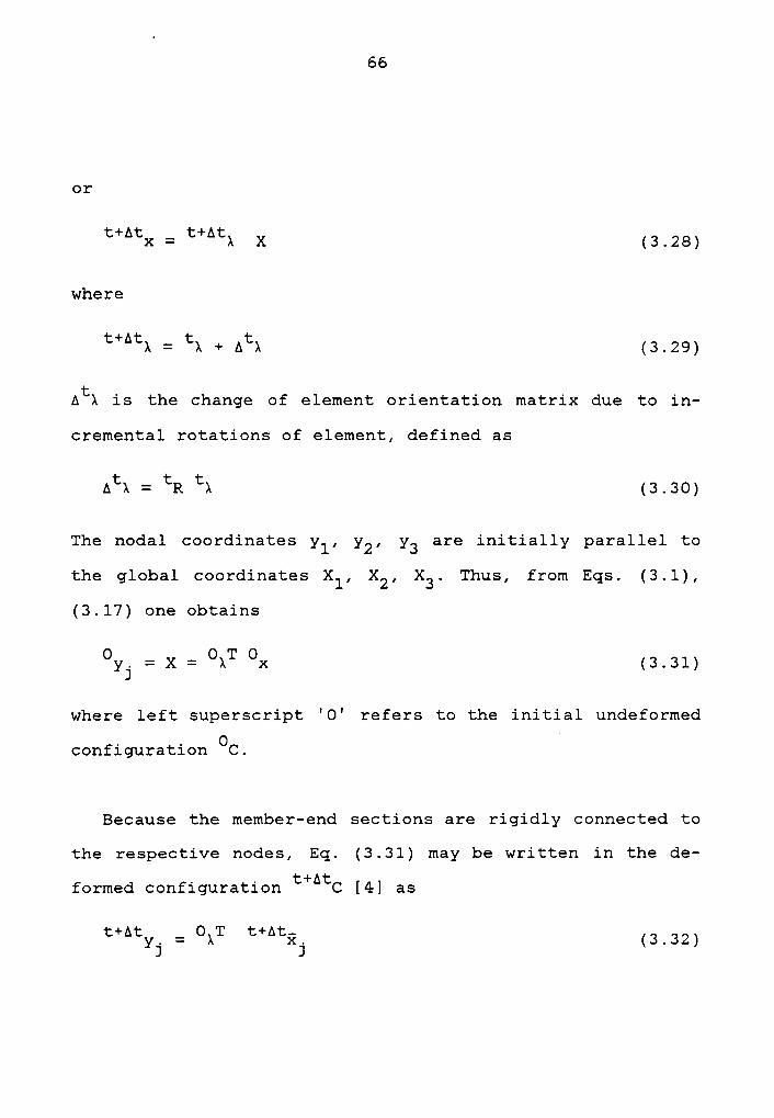
t+^tx = t+^tx x (3.28)
where
t+^tx = tx + Atx (3.29)
Atx is the change of element orientation matrix due to in-
cremental rotations of element, defined as
Atx = tR tx (3.30)
The nodal coordinates yl, y2, y3 are initially parallel to
the global coordinates X1, X2, X3. Thus, from Eqs. (3.1),
(3.17) one obtains
Oyj = x = Ox": Ox (3.31)
where left superscript 'O' refers to the initial undeformed
configurationOC.
Because the member—end sections are rigidly connected to
the respective nodes, Eq. (3.31) may be written in the de-
formed configuration t+AtC [4] as
t+Atyj = OXT t+Atäj (3.32)

67
t+At• . . _where xj is the coordinate vector of end section at nodej in the t+AtC configuration.
From Eqs. (3.32),(3.14),(3.l7) one obtains
t+^t ij « 0; t+Atyj „ Ol t+^t°j
X(3.33)
Since deformations are small
.. ! • • 3 1S1n eJn eau , COS eJn (3_34)
where ejn is the relative element rotation at node j about
xn-axis.
From Figs. 3.1 and 3.3 one obtains
1 c¤s(90' - ejg) cos(90° + ejz)mt ij · ¢¤s( 9¤‘ + eig) 1 cos(90' z •t/2) ‘*^tx
' cos( 90' - ejz) cos(90° : gt/2) 1
(3.35)
where j is 1 for the left end and 2 for the right end; ejz,
ej3 are the relative end rotations at node j about the x2,
x3-axes respectively, ¢t is the relative angle of twist of
the element ends about the xl—axis, and the upper and lower
signs apply to nodes 1 and 2, respectively.
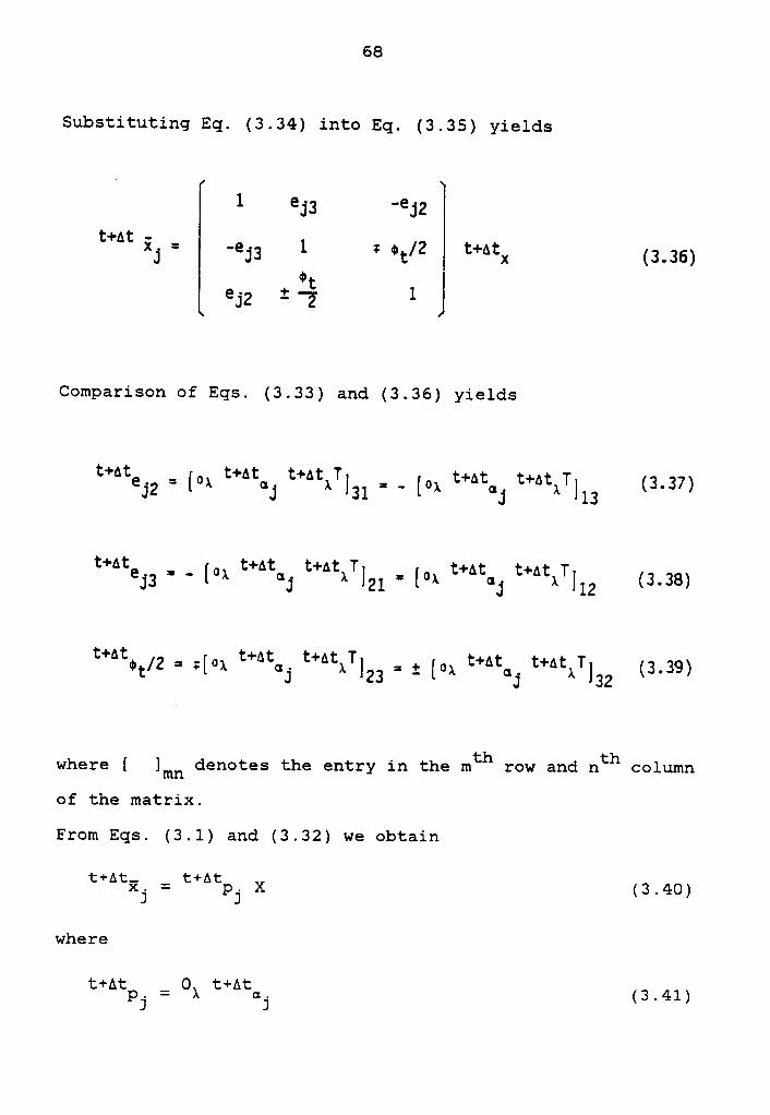
68
Substituting Eq. (3.34) into Eq. (3.35) yields
1 Ejg -€j2t+At ·
_xj — —ej3 1 = ¢t/2 t+Atx (3.36)
°·cEjz I 1
Comparison of Eqs. (3.33) and (3.36) yields
t+At2j2 2 2 (3-37)
t+At 2 _ t+At t+At T t+At t+6t Taj} [°* ¤j 1 ]2l == [°x aj A ]12 (3.38)
t+6t t+6t t+6t T t+At t+ t T2 = 0-
=where[ Imn denotes the entry in the mth row and nth column
of the matrix.
From Eqs. (3.1) and (3.32) we obtain
t+^t2. = t+^tp. x (3.40)J J
where
t+Atpj 2
69
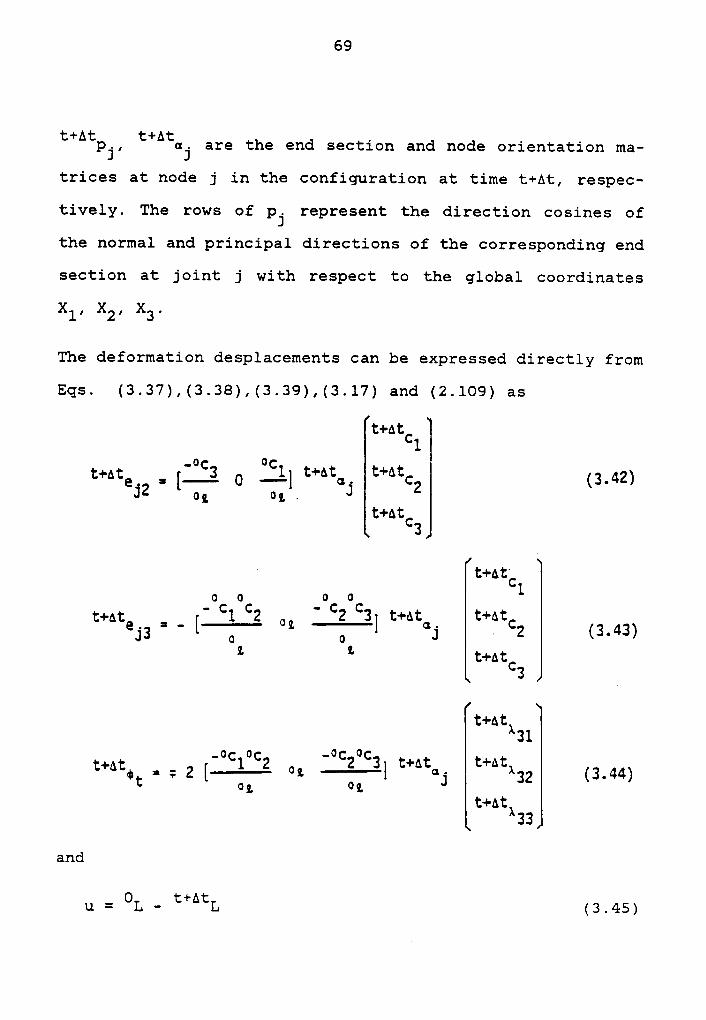
t+Atpj, t+At¤j are the end section and node orientation ma-trices at node j in the configuration at time t+At, respec-
tively. The rows of pj represent the direction cosines of
the normal and principal directions of the corresponding end
section at joint j with respect to the global coordinates
xl, X2, X3.
The deformation desplacements can be expressed directly from
Eqs. (3.37),(3.38),(3.39),(3.l7) and (2.109) as
:+6:°1
, 0t+A‘Ce _[ °°3 0 :+6:cz (BM)
jz 0; Og . J
:+6:°3
· t+ACtOC Oc Oc Oc 1
:+6: ' 1 2 0 ° 2 3 :+6: :+6:Q. ·———- 9. —-T- a. C
J3S [
6 oz]
J · 2 (3.43)
'- :+6:°3
:+6:l3l-0; 0; -0; 0;
:+6: 1 2 2 3 :+6: t+ACX=;z ——— ¤z —i} ¤- 3.44°: [ 6, 66 .1 32 ( )t+AtX
33
and
u = O1. — t+^”°L(3.45)
Chapter IV
FINITE ELEMENT MODEL
4.1 INTRODUCTION
To solve the incremental equilibrium equation in the U.L.
formulation we must to evaluate the finite element matrices
in Eq. (2.55). The local element secant stiffness matrix of
the plane frame element, developed by Katzenberger [48], is
extended to form the local element secant stiffness matrix
of the space frame element in which the torsional forces are
treated independently and obtained by linear theory.
For a straight small strain beam of constant cross sec-
tion in the convected coordinate system, Hermitian interpo-
lation functions are employed to interpolate the transverse
bending displacements, and Lagrange interpolation functions
are used to interpolate the axial and torsional displace-
ments [9],[33],[34].
For convenience, the left superscripts and subscripts are
not shown in this formulation.
70
71
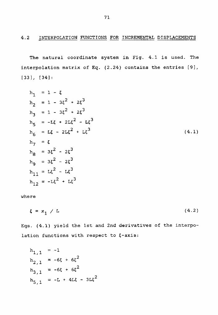
4.2 INTERPOLATION FUNCTIONS FOR INCREMENTAL DISPLACEMENTS
The natural coordinate system in Fig. 4.1 is used. The
interpolation matrix of Eq. (2.24) contains the entries [9],
[33], [34]:
hl = 1 —E
hg =1-2;2+2;3hg =1-3;2+2;3hg = -L; + 2L;2 — L;3
_ 2 3h6 — LZ - 2LZ + LZ (4.1)
h7 = ;_ 2 _ 3h8 - 3E 2E
hg = s;2 — 2;3_ 2 _ 3
hll— Li LZ_ _ 2 3
hlg — LZ + LZ
where
; = xl / L (4.2)
Eqs. (4.1) yield the 1st and 2nd derivatives of the interpo-
lation functions with respect to ;-axis:
hl,l = '1h = -6; + 6;22,1
_ _ 2hgll - 6; + 6;
_ 2hgll — -L + 4L; 3L;
72
h6ll = L — 4L; + 3L€2(4.3)
h7’1 = 1
11 = 6E - 6;28,1
119,1 = 6i - 6;2
11119 = 211; — 3L£2hlzil = -2LE + 3L£2
and
hzill = -6 + 12;
h3 ll = -6 + l2£
hslll = 4L - 6L£
hölll = -4L + 6LE
hglll = 6 - 12E (4.4)
hglll = 6 - 12E
hlllll = 2L - 6L;
hlzlll = -2L + 6L;
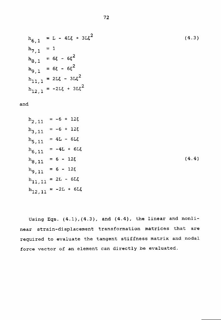
Using Eqs. (4.l),(4.3), and (4.4), the linear and nonli-
near strain-displacement transformation matrices that are
required to evaluate the tangent stiffness matrix and nodal
force vector of an element can directly be evaluated.
73- A
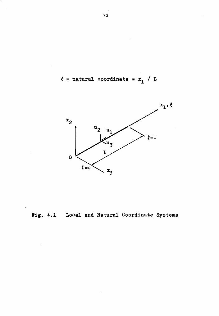
6 = natural coordinate = xl / L
Xlog
X2u
2
*6. LO$=0
*6
Fig. 4.1 Local and Natural Coordinate Systems
74
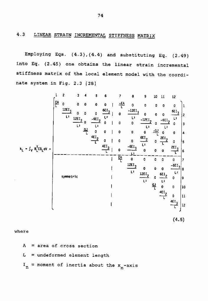
4.3 LINEAR STRAIN INCREMENTAL STIFFNESS MATRIX
Employing Eqs. (4.3),(4.4) and substituting Eq. (2.49)
into Eq. (2.45) one obtains the linear strain incremental
stiffness matrix of the local element model with the coordi-
nate system in Fig. 2.3 [28]
1 2 3 4 5 6 7 6 9 10 11 12
ä 0 0 0 0 0 | 0 0 0 0 0 11261 661 -1261 6610 0 0 -——E| 0 -—-—! 0 0 0 ———E 21261 -661 L2 L’
-1261 -661 L2———! 0 -—-! 0 | 0 0 -—-—! 0 -—-! 0 3v L2 L= wEQ 0 0 | 0 0 0 SEQ 0 0 44EI 661 261—T! 0 | 0 0 —-! 0 jr! 0 s
T 4613 -6613 LZ 2613RL ' IV BLEBLdV ' —__——_____——__**il_2——iLL—_(L——(L_(L—_T_ 6
| EQ 0 0 0 0 0 71261 -661| ———E 0 0 0 ———E6L’
12EIz 6EIz L'symetric | —— 0 0 9.
L3 |_2
| EQ 0 0 104U| —j! 0 11
ar| —j! 12
. (4.5)
where
A = area of cross section
L = undeformed element length
In = moment of inertia about the x¤—axis
· 75
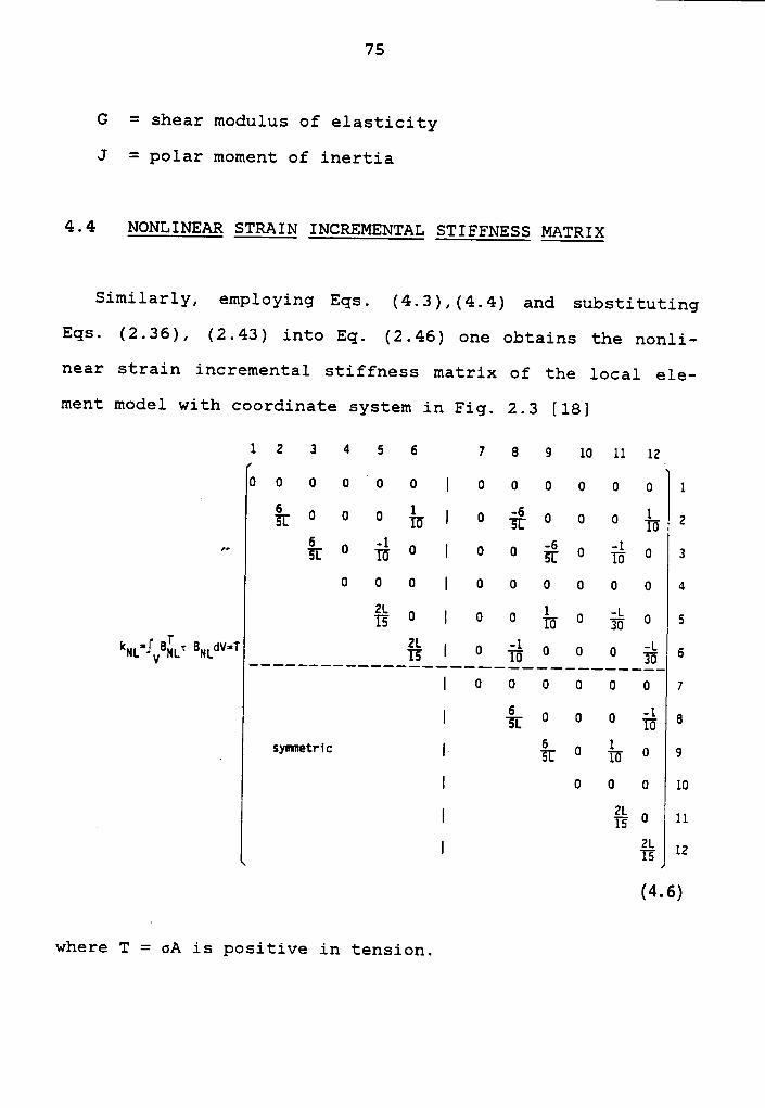
G = shear modulus of elasticity
J = polar moment of inertia
4.4 NONLINEAR STRAIN INCREMENTAL STIFFNESS MATRIX
Similarlyy employing Eqs. (4.3),(4.4) and, substituting
Eqs. (2.36), (2.43) into Eq. (2.46) one obtains the nonli-
near strain incremental stiffness matrix of the local ele-
ment model with coordinate system in Fig. 2.3 [18]
1 2 3 4 6 6 7 6 9 10 ll 12*0 0 0 0 °0 0 | 0 0 0 0 0 0 1u
Q5 0 0 0 {5 | 0 5% 0 0 0 1% 2„ QT 0 {-5 0 | 0 0 ff 0 {5 0 3
0 0 0 | 0 0 0 0 0 0 4
{5 0 | 0 0 {-5 0 ä 0 s6
| 0 0 0 0 0 0 7
| §5 0 0 0 {5 6*
symetric |- gt 0 {5 0 9
| 0 0 0 m
| % 0 11| {5 12
(4.6)
where T = oA is positive in tension.
1 76
The nonlinear strain incremental stiffness matrix RNL isindependent of elastic properties. It depends only on the
element's geometry, displacement field, and the current
state of stress level.
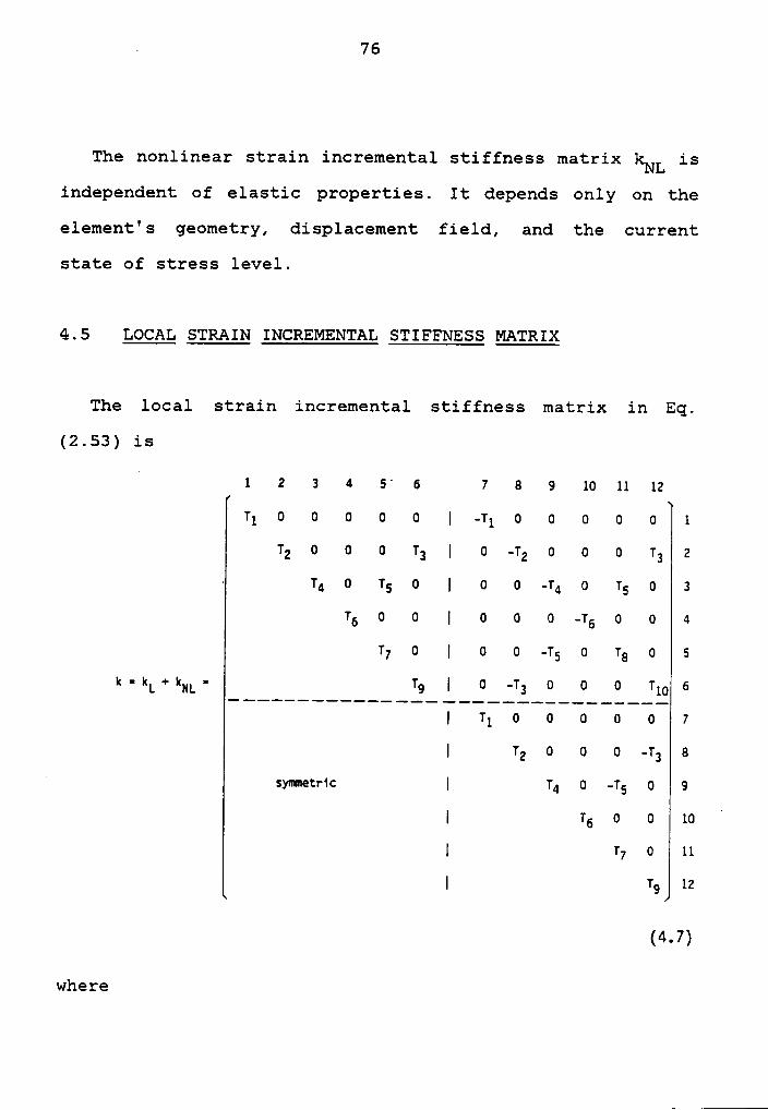
4.5 LOCAL STRAIN INCREMENTAL STIFFNESS MATRIX
The local strain incremental stiffness matrix in Eq.
(2.53) is
1 2 3 4 6* 6 7 6 9 10 11 12
T1 0 0 0 0 0 | -T1 0 0 0 0 0 1
T2 0 0 0 T3 | 0 -T2 0 0 0 T3 2~ T4 0 T6 0 | 0 0 -T4 0 T6 0 3
T6 0 0 | 0 0 0 -T6 0 0 4
T7 0 | 0 0 -T6 0 T6 0 5
k = k1 + kNL · T3 | 0 -T3 0 0 0 T10 6
| T1 0 0-0-
0v0-
7
| T2 0 0 0 -T3 6
symetri c | T4 0 -T6 0 9
{ T6 0 0 10 '
| 5 0 u
| 5 M
(4.7)
where
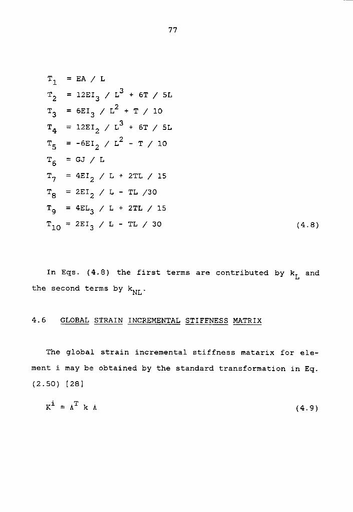
77
Tl = EA / L
T2 = l2EI3 / L3 + 6T / 5L_ 2T3 — 6EI3 / L + T / 10_ 3T4 — 12EI2 / L + 6T / 5L-_ 2_T5 — 6EI2 / L T / 10
T6 = GJ / L
T7 = 4EI2 / L + 2TL / 15
T8 = 2EI2 / L — TL /30
Tg = 4EL3 / L + 2TL / 15
T10 = 2EI3 / L — TL / 30 (4.8)
In Eqs. (4.8) the first terms are contributed by kL and
the second terms by kNL.
4.6 GLOBAL STRAIN INCREMENTAL STIFFNESS MATRIX
The global strain incremental stiffness matarix for ele-
ment i may be obtained by the standard transformation in Eq.
(2.50) [28]
1<i=ATkA (4.9)
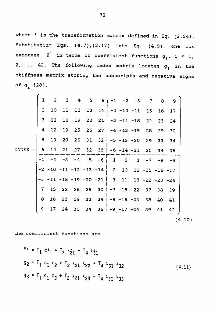
78
where A is the transformation matrix defined in Eq. (2.54).
Substituting Eqs. (4.7),(3.17) into Eq. (4.9), one can
exppress Ki in terms of coefficient functions gi, i = 1,
2,.... 42. The following index matrix locates gi in the
stiffness matrix storing the subscripts and negative signs
of gi [28].
1 2 3 4 5 6| -1 -2 -3 7 8 9I2 10 11 12 13 14I -2 -10 -11 15 16 17
3 11 18 19 20 21 :-3 -11 -18 22 23 244 12 19 25 26 27: -4 -12 -19 28 29 305 13 20 -26 31 32 :-5 -13 -20 29 33 34
INDEX = 6 14 21 27 32 35 |-6 -14 -21 30 34 36
-1 -2 -3 -4 -5 -6| 1 2 3 -7 -8 -9
-2 -10 -11 -12 -13 -14: 2 10 11 -15 -16 -17-3 -11 -18 -19 -20 -21: 3 11 18 -22 -23 -24
7 15 22 28 29 30I -7 -15 -22 37 38 39I
8 16 23 29 33 34| -8 -16 -23 38 40 41I9 17 24 30 34 36| -9 -17 -24 39 41 42
(4.10)
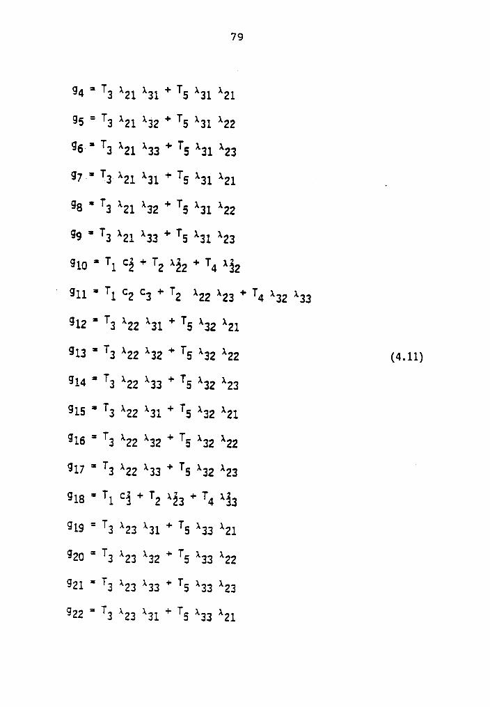
the coefficient functions are
g=1 Tl czl + T2 xäl + T4 xäl
C2 ’ T1 C1 C2 * T2 *21 *22 * T4 *21 *22 (4.11)= TC3 1 C1 C2 * T2 *21 *22 * T4 *21 *22
79
94 * T2 *21 *21 * Ts *21 *2195 * T2 *21 *22 * Ts *21 *22962* T2 *21 *22 * Ts *21 *22g7‘= T2 *21 *21 * Ts *21 *21 .98 * T2 *21 *22 * Ts *21 *2299 * T2 *21 *22 * Ts *21 *22Q10 * T1 92 * T2 *22 * T4 *22
T 911 * T1 92 92 * T2 *22 *22 * T4 *22 *22912 * T2 *22 *21 * Ts *22 *21913 * T2 *22 *22 * Ts *22 *22 (4-11)914 * T2 *22 *22 * Ts *22 *22915 * T2 *22 *21 * Ts *22 *21916 * T2 *22 *22 * Ts *22 *22917 * T2 *22 *22 * Ts *22 *22918 * T1 92 * T2 *22 * T4 *22919 * T2 *22 *21 * Ts *22 *21920 * T2 *22 *22 * Ts *22 *22921 * T2 *22 *22 * Ts *22 *22922 * T2 *22 *21 * Ts *22 *21

80
923 ' T2 *22 *22 * Ts *22 *22 .924 ’ T2 *22 *22 * Ts *22 *22925 ’ T6 9i * T9 *21 * T7 *21 _926 ' T6 91 92 * T2 *21 *22 * T7 *21 *22927 ‘ T6 91 92 * T2 *21 *22 * T7 *21 *22
928 ' ‘ T6 9i * T10 *21 * T6 *21929 ‘ ‘T6 91 92 * T10 *21 *22 * Ta *21 *22930 ’ ‘T6 91 92 * T10 *21 *22 * T6 *21 *22
~ 931 ’ T6 92 * T2 *22 * T7*22932‘ T6 92 92 * T2 *22 *22 * T7 *22 *22
933 ‘ ‘T6 92 * T10 *22 * T6 *22934 ‘ ‘T6 92 92 * T10 932933 * Ta *22 *22935 ’ T6 92 * T9 *22 * T7 *22935 ‘ ‘T6 92 * T10 *22 * T6 *22937 ’ T6 92 * T9 *21 * T7 *21938 ‘ T6 91 92 * T92931 *22 * T7 *21 *22939 ‘ T6 91 92 * T9 *21 *22 * T7 *21 *22940 ’ T6 92 * T9 *22 * T7 *22941 ’ T6 92 92 * T2 *22 *22 * T7 *22 *22942 ‘ T6 92 * T2 *22 * T7 *22
81
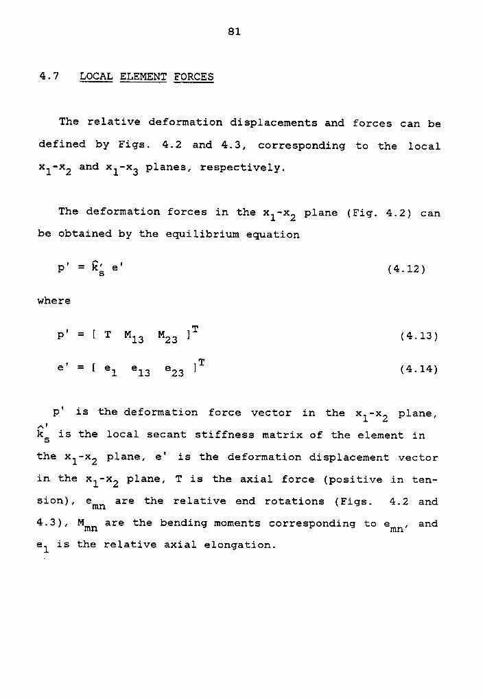
4.7 LOCAL ELEMENT FORCES
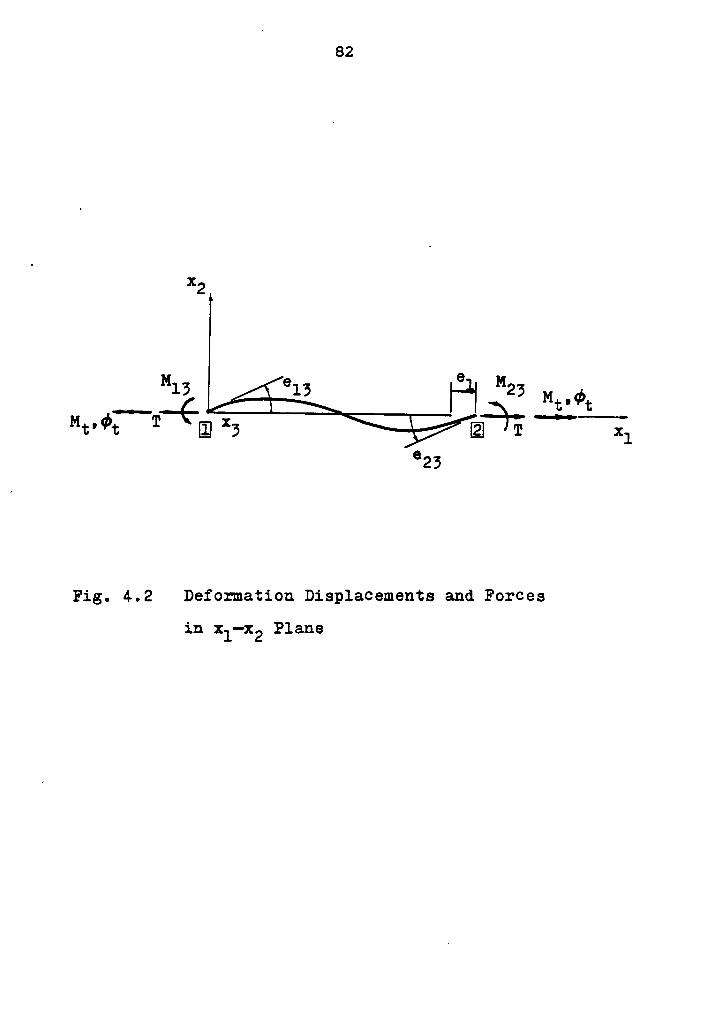
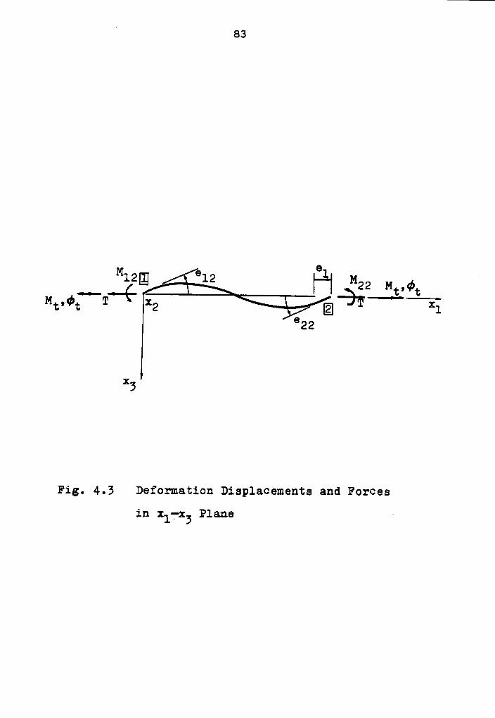
The relative deformation displacements and forces can be
defined by Figs. 4.2 and 4.3, corresponding to the local
xl-x2 and xl-x3 planes, respectively.
The deformation forces in the xl-x2 plane (Fig. 4.2) can
be obtained by the equilibrium equation
p' = Hg e' (4.12)
where
p' = [ T M M ]T(4 13)13 23 '
|_
Te — [ el e13 e23 ] (4.14)
p' is the deformation force vector in the xl-x2 plane,I
QS is the local secant stiffness matrix of the element inthe xl—x2 plane, e' is the deformation displacement vector
in the xl·x2 plane, T is the axial force (positive in ten-
sion), emn are the relative end rotations (Figs. 4.2 and
4.3),Mmn
are the bending moments corresponding toemn,
and
el is the relative axial elongation.
82
*2
6M15 815 t-J-I M25 Mt_¢tM·c·¢t T li! *5 121 TT xl
°25
Fig. 4.2 Deformation Displacements and Forces
in xl-x2 Plane
° es
M12 912 alM ‘
6 |"| B22 Mw.°22
xs
Fig. 4.5 Deformation Displacements and Forces
in xlrxj Plane ·
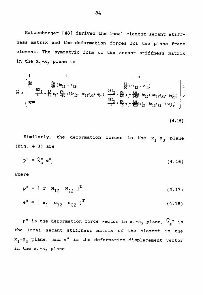
84
Katzenberger [48] derived the local element secant stiff-
ness matrix and the deformation forces for the plane frame
element. The symmetric form of the secant stiffness matrix
in the xl-x2 plane is
1 2 l3
gg EA ML ä ("*12 ' *22) E5 ("*22 ’*12) 1
Fig- &+EAe+%(12e 3ee+ )ä EA +£3 4L T5 1 420 i2‘ 13 23 *52 L ‘ E *1 840(” *12* *12*22‘ 3*22) 2sym ä + E^ + 2 + 12 1 2L T5 *1 420 *i2° *12*22 *52) j
(4.15)
Similarly, the deformation forces in the xl-x3 plane
(Fig. 4.3) are
p" = ü; e"' (4.16)
where
p" = [ T M M 1T(4 17)12 22 °
e" = [ e e e ]T(4 18)1 12 22 '
Ap" is the deformation force vector in xl-x3 plane, kS" isthe local secant stiffness matrix of the element in the
xl-x3 plane, and e" is the deformation displacement vector
in the xl-x3 plane.

85
Comparing Fig. 4.2 with Fig. 4.3, we obtain the local
element secant stiffness matrix in xl—x3 plane, similar toEq. (4.15): _
1 4 5EA EA [T m BU ("*12 ‘ *22)
BE€'1"*22 ‘ *12) *1- ZEI"’°
' * 1% *1* %(1**1z° 3*12*22* *22) T3 ‘ gg *1* %(‘3*i2* ‘*12*22‘3*§2)‘
sm mz+ EA EL ,
1 T5 *1* 4201*12**)*12*22* 1**22) 5
(4.19)
Combining Eqs. (4.12) and (4.16), one obtains the deforma-
tion forces of the space frame element
— {2p —S e (4.20)
where
= Tp [ T M13 M23 M12 M22 ] (4.21)
= Te [ el e13 e23 elz e22 ] (4.22)
p, e are the deformation force and displacement vectors of
the space frame element, respectively.
The relative element forces and displacements are as
shown in Fig. 4.4. The superposition of Eqs. (4.15) and
(4.19) in accordance with the sequence in Eqs. (4.21) and

‘ 86
xl•
M22’€22 AtX2 }/T,el
[Z]
“12·°12 {=$·\ M16•°16E*6
Fig. 4.4 Relative Element Forces and‘Displacements
in Space Frame Element

87
(4.22) yields the local element secant stiffness matrix of
space frame
1 2 3IEA EA I*^"· an '6?5I"'*13 ' *23) zu B6 I"*23 ‘ *13) }EA 3 EA EAL 3 EA EA1 ‘
3b’I‘*13’ *23) T * T5 *1* ¤öIl**i3'**13*23**23) T ' 56*1* §EI°**i3*“*13*23‘**23)I· EA ***3 EA EAL ‘*‘3 EA EA1 '"s’ Bb‘I‘*23'*13) T ‘ Kö *1* W[°3°i3+4°13°23” **23)T * T5 *1* mI*i3‘**13*23*1**ä3)IEA I1 55 I"*12 ‘ *22) °°EA I
E5 I“*22' *12)° ° I
EA EAI B5 I“*12' *22) E I"*22‘ *12) II 0 0 ‘ 2I 0 0 3
***2 EA EAI. 2**2 EA EALIE * E *1* II**i2' **12*22* *22) T ‘ BB *1* I‘**f2* "*12*22‘ **22) “‘
2 EA EA1 ***2 EA EA1 ,I 1 ° 56 *1* I‘**i2* "*12*22' **22) T * T5 *1* Téö I*i2‘ **12*22*‘**22) S
(4.23)
From equilibrium conditions one obtains the local element
forces corresponding to Fig. 2.3:
fl = -T
88
fz = (M13+M23) / Lf3 = '(M12+M22) / Lfs = M12fö = M13f7 = —fl
f8 = —f2
fg = -f3
fll = M22flz = M23 (4.24)
The torsional forces are treated independently and can be
obtained from the linear theory [28]
f4 = ·(GJ/L) ¢t
flo = -f4 (4.25)
where ¢t is the relative rotation of element ends about the
element axis.
4.8 GLOBAL ELEMENT FORCES
The global element forces for element i can be obtained
from Eq. (2.51):
Fi = AT f (4.26)
where A is defined in Eq. (3.17). The components of Fi are

89
F1 = Clfl+x21f2+X31f3
F2 : c2fl+X22f2+x32f3
F3 = c3fl+k23f2+Ä33f3
F4 = Clf4+x2lf5+X3lf6
F5 = C2f4+x22f5+X32f6
F6 = c3f4+x23f5+x33f6
F7 = °1f7+x21f6+x31f9
F6 = C2f7+x22f8+x32f9
F9 = °3f7+F22f6+x33F9
F10 = °1f10+x21F11+“31F12
F11 = c2f10+x22fll+x32f12
F12 = c3flO+X23fll+Ä33fl2 (4‘27)
Chapter V
BEAM-COLUMN MODEL
5.1 INTRODUCTION
This chapter presents the three-dimensional beam-column
model in U.L. formulation [2],[4], which is based on the
conventional beam—column theory [23]. Because using the ac-
tural solution to the differential equation, the beam-column
model can trace equilibrium path accurately. In this model
the behavior of the element is referred to the convected
coordinate system, and then a transformation is applied from
a local to a global coordinate system.
The rotations and translations of the nodes are consid-
ered to be arbitrarily large, but the relative deformations
of the element are assumed to be small such that the conven-
tional beam-column theory can be applied. In the beam-column
model, the effect of length shortening due to bending is
considered, and the external loads are supposed to be ap-
plied at the nodes only.
90
91
5.2 ELEMENT END FORCE-DEFORMATION RELATIONS
The relationships between element-end forces and deforma-
tions (Fig. 5.1) based on the conventional beam—column theo-
ry are (2l,l3].l23l=
Mln = Eln / L (clneln +c2ne2n) (5'l)
M2n = EIn / L (c2ne1n + C1ne2n) (5'2)
Mt = (GJ / L) ¢t (5.3)
P = EA (u / L - cbz - cb3) (5.4)
in which
emn = relative end rotations (Fig. 5.1); the first sub-
script refers to the node where the angle is mea-
sured (1 for left node and 2 for right node); the
second subscript indicates the axis about which the
rotation takes place
Mmm = bending moment corresponding to emnMt = torgue
P = axial force, positive in compression
cmn = stability functions [1],[4] associated with
bending moments about the xn-axis (Appendix B)
L = element length
u = relative axial displacement
92
cbn is length correction factor resulting from the flexural
deformations about the xn-axis [l],[Z] defined as
Q =b (Q +Q )2+b (Q -Q )2 (55)bn ln ln Zn Zn ln Zn '
bln, bznare the bowing functions given by
b = (c +c )(c -2) / 8 nzpln ln Zn Zn n
bzn = czn / 8(cln+c2n) (5.6)
in which
pn = P / PE¤ - (5.7)
pn is the dimensionless axial force parameter and
_ 2 2PE¤ — n E In / L (5.8)
Thus
pn = 121.2 / nz E in (5.9)
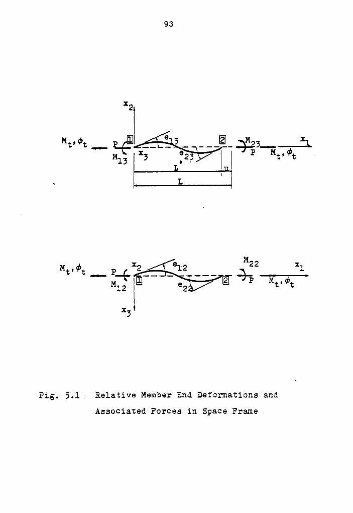
93
XZI
8”¤·"’¤..- Lg? -- -3-----2-- .;*226...-;.M :3 623
I
'
P .13 •
·L
I
. L
Mx 6. 22 :“¤"2t-.. Lg, 2.{i22 --- .;. .....i.P26
Fig. 5.1. Relative Member End Deformations and
Associated Forces in Space Frame

94
5.3 TANGENT STIFFNESS MATRIX FOR RELATIVE DEFORMATIONS
The relation between incremental vectors, the relative
end forces and deformations is
A bc— e ( . )f — Q A s 10
where
_ TAfbc — [ AMl3 AM23 AMl2 AM22 AMt APL ]
Ae = [ Ael3 Ae23 Aelz Aezz A¢t Au/L IT (5.11)
is the tangent stiffness matrix for relative deforma-
tions of the beam-column model and has been derived by Oran
[2]:
Gis 613623 @13‘2°1s* M ‘a°2a* M °
G G T
G13G23 623G33‘2°22* M £3C13+
° ° ° T
0 0 0 G12‘2°12 M M T
(5.12)~ EI G12G22 Gäz Gk = T 0 0 52:22+ 52c12+OÜ
Ü Ü Ü n Q
E E E 2; 0 .2H H H H T'
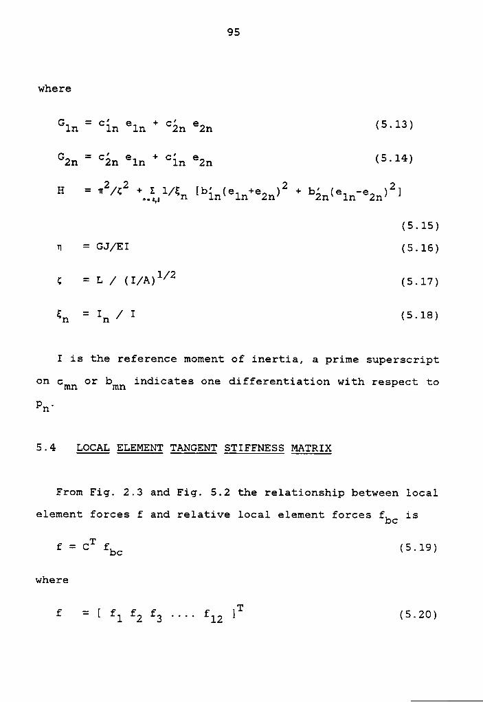
95
where
Gln = cln eln + c2n€2n
(5°l3)
Gzn = °2n eln + cln °2n (S14)
_ 2 2 , 2 , _ 2He2n) 1
(5.15)
H = GJ/EI (5.16)
c = L / <1/A>l/2 (5-17)
En = In / 1 (5.18)
I is the reference moment of inertia, a prime superscript
on cmn or bmn indicates one differentiation with respect to
Pn-
5.4 LOCAL ELEMENT TANGENT STIFFNESS MATRIX
From Fig. 2.3 and Fig. 5.2 the relationship between local
element forces f and relative local element forces fbc is
6 = cT6bc (5.19)
where
£ = [ f f E f 1T(5 20)
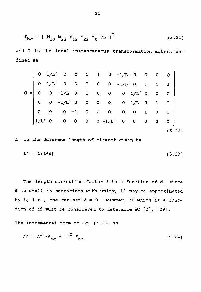
96
_ Tfbc - [ M13 M23 M12 M22 Mt PL ] (5.21)
and C is the local instantaneous transformation matrix de-
fined as
O 1/L' O O O 1 O -1/L' 0 O O O
O 1/L' O O 0 O O -1/L' O O O 1
C = O O -1/L' O 1 O O O 1/L' O O O
O O -1/L' 0 O O O O 1/L' O 1 O
O O O -1 O O O O O 1 O O
1/L' O O O O 0 -1/L' O O O O O
(5.22)
L' is the deformed length of element given by
L' = L(1+6) (5.23)
The length correction factor 6 is a function of d, since
6 is small in comparison with unity, L' may be approximated
by L; i.e., one can set 6 = O. However, A6 which is a func-
tion of Ad must be considered to determine AC [2], [29].
The incremental form of Eq. (5.19) is
Af = cT Asbc + AcT fbc (5.24)
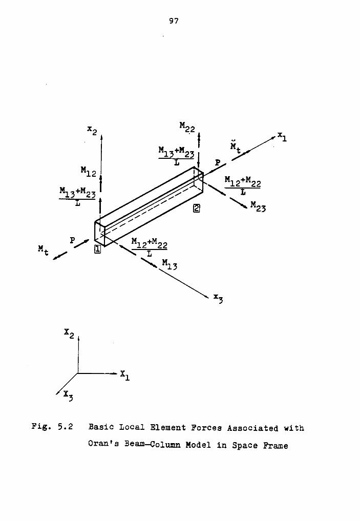
97
Mx 22I
2I ii
lxl1413+142: t
ML I P
12 M +M12 22M +M L13 23
I Q M234
P/' E} M12*M22Mt III\
M
*3
M2
X1M3
Fig. 5.2 Basic Local Element Forces Associated with
Oran's Beam-Column Model in Space Frame
98
where AC is the change in C resulting from Ad (see Appendix
C)
By contragredience from Eq. (5.19)
Ae = C Ad (5.25)
Substituting Eqs. (5.10), (5.25), (C.1) into Eq. (5.24), one
obtain
Af = k Ad (5.26)
where k is the local tangent stiffness matrix of element de-
fined as
k = kL + RNL (5.27)
where
TA .kL = C k C (5.28)
= Q f gn) (5.29)kNLi=1 bci
kL’ kNL are the linear and nonlinear tangent stiffness ma-
trix respectively, g(i) are the geometric matarices defined
in appendix C.
Substituting Eqs. (5.12),(5.22) into Eq. (5.28), one can ex-
press the kL in terms of coefficient functions gi, i =
l,....20:
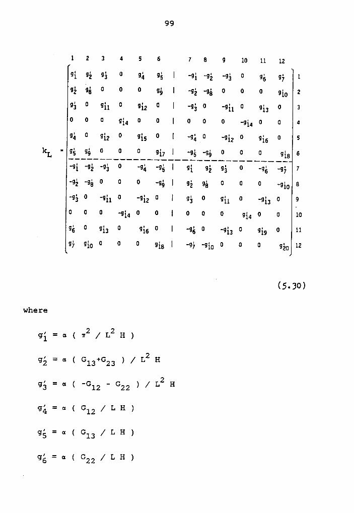
99
”123456 769101112Qi Qé 9ä 0 95 Qé I -95 -95 -95 0 Qé 95 1
0é0é°°°0éI·0é·0é°°°0i830ä
° 011 ° 0iz ° I -010 ·0i1° 018 °
30 0 0 954 0 0 I 0 0 0 -954 0 0 4gi
° giz °gis
° I ‘gÄ_° 'giz°
gis°
5kL*9é9§0 0 0 957I-95-950 0 0 9556
-95 -95 -95 0 -95 -95 I 9i 95 Qä 0 -95 -95 7
-01-080 ° °·0éI 0101
° ° ° -0183‘gä°
°gi10 'giz ° I gä° gi1 °
‘gia°
90 0 0 -954 O 0 I O 0 0 954 0 0 10gs
°gis
° gis °I ‘gs
° 'gis °gis
°III
01 018 0 0 0 018 I -0% -0111 0 0 0 018 I3
‘ (5•3¤)
where
295 = 8 < 82 x L H >g’=a(G+G )/LZH2 13 23
g'=a(-G -G )/LZH3 12 22
9j5=¤=(Gl2/LH)
95=¤=(Gl5/LH)
I —q6—¤(G2_-5/LH)
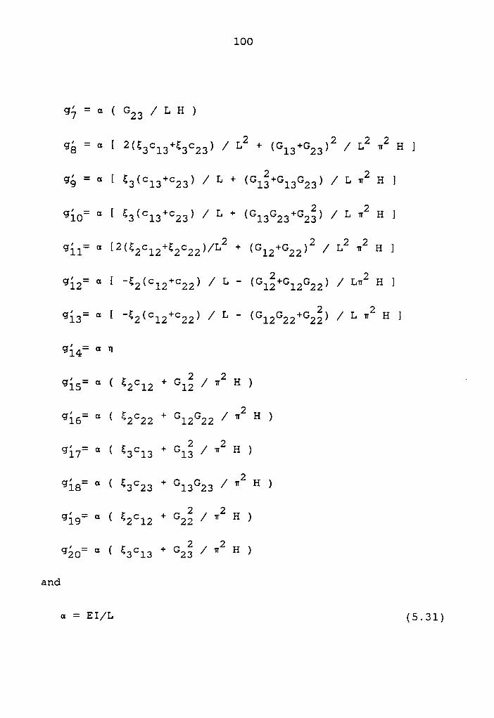
100
9’·}=¤=(G23/LH)
gé : g L2 + (Gl3+G23)2 / L2 “2 H 1
gé L + (G1§+G1sG2s) / L "2 H ]
gio: g L + (G1sG2s+G2§) / L “2 H 1
Has H H Hgiz: g L L“2 H 1
gis: g [ 'g2(°12+°22) / L L “2 H 1
gi4: ° "gis: g ( g2°12 + Giä / “2 H ) L
gi6: g ( €2C22 + Gl2G22 / “2 H )
giv: "2 H )
gis: ° ( gsczs + G13G23 / “2 H )
H1g= H H >géo: ° ( gscis + Gzä / “2 H )
amd
„ = E1/L (5.31)
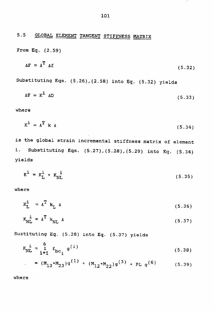
101
5.5 GLOBAL ELEMENT TANGENT STIFFNESS MATRIX
From Eq. (2.59)
AF = AT Af (5.32)
Substituting Eqs. (5.26),(2.58) into Eq. (5.32) yields
AF =Ki AD (5.33)
where
Ki = AT K A (5.34)
is the global strain incremental stiffness matrix of element
i. Substituting Eqs. (5.27),(5.28),(5.29) into Eq. (5.34)
yields
Ki = Ki + KN; (5.35)where
Kä = AT KL A (5.36)
KNä = AT KNL A (5.37)Sustituting Eq. (5.28) into Eq. (5.37) yields
KNä = igl sbci g(T) (5.38). = (M13+M23)g(T) + (Ml2+M22)g(3) + pg g(6) (5.39)
where
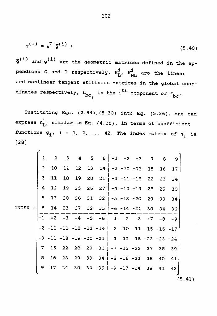
102
gu) = AT §(T) A (6.40)§(i) and g(i) are the geometric matrices defined in the ap-
pendices C and D respectively. Kä, K;L are the linearand nonlinear tangent stiffness matrices in the global coor-
dinates respectively, fbci is the ith component of fbc.
Sustituting Eqs. (2.54),(5.30) into Eq. (5.36), one can
express Ki, similar to Eq. (4.10), in terms of coefficient
functions gi, i = 1, 2,.... 42. The index matrix of gi is
[28]
1 2 3 4 5 6 :-1 -2 -3 7 8 92 10 11 12 13 14 :-2 -10 -11 15 16 173 11 18 19 20 21 :-3 -11 -18 22 23 244 12 19 25 26 27 :-4 -12 -19 28 29 30
5 13 20 26 31 32 :-5 -13 -20 29 33 34
INDEX = 6 14 21 27 32 35 :-6 -14 -21 30 34 36
-2 -10 -11 -12 -13 -14 : 2 10 11 -15 -16 -17
-3 -11 -18 -19 -20 -21 : 3 11 18 -22 -23 -24
7 15 22 28 29 30 :-7 -15 -22 37 38 39
8 16 23 29 33 34 :-8 -16 -23 38 40 41
9 17 24 30 34 36 :-9 -17 -24 39 41 42
(5.41)
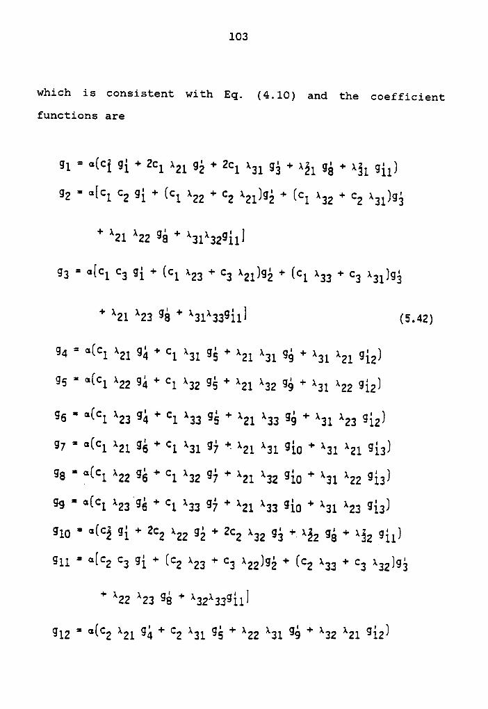
103
which is consistent with Eq. (4.10) and the coefficient
functions are
91 9 9*91 91 9 991 *21 92 9 991 *31 93 9 *21 93 9 *31 911*92 9 9*91 92 91 9 *91 *22 9 92 *21*92 9 *91 *32 9 92 *31*93
9 *21 *22 93 9 *31*32911*
93 9 9*91 93 91 9 *91 *23 9 93 *21*92 9 *91 *33 9 93 *31*939 *21 *23 93 9 *31*33911* (5-42)
94 9 9*91 *21 93 9 91 *31 93 9 *21 *31 93 9 *31 *21 912*95 9 9*91 *22 93 9 91 *32 93 9 *21 *32 93 9 *31 *22 912*96 ‘ 9*91 *23 93 9 91 *33 93 9 *21 *33 93 9 *31 *23 912*97 ' 9*91 *21 93 9 91 *31 91 9 *21 *31 910 9 *31 *21 913*96 ‘ 9*91 *22 93 9 91 *32 91 9 *21 *32 910 9 *31 *22 913*99 ' 9*91 *23 93 9 91 *33 91 9 *21 *33 910 9 *31 *23 913*910 9 9*92 91 9 992 *22 92 9 992 *32 93 9 *22 93 9 *32 911*911 9 9*92 93 91 9 *92 *23 9 93 *22*92 9 *92 *33 9 93 *32*93
9 *22 *23 93 9 *32*33911*
g12S °*C2
921 93 + C2 931 gg + 922 X3], gé + 932 921 932)

104
913 9 9192 *22 91 9 92 *22 96 9 *22 *22 95 9 *22 *22 912)914 9 9192 *22 91 9 92 *22 96 9 *22 *22 95 9 *22 *22 912)915 9 9192 *21 96 9 92 *21 91 9 *22 *21 910 9 *22 *21 912)916 9 9192 *22 96 9 92 *22 91 9 *22 *22 910 9 *22 *22 912)917 9 9192 *22 96 9 92 *22 91 9 *22 *22 910 9 *22 *22 912)918 9 9192 91 9 292 *22 92 9 292 *22 96 9 *22 96 9 *62 911)916 9 9192 *21 91 9 92 *21 96 9 *22 *21 95 9 *22 *21 912)920 9 9192 *22 91 9 92 *22 96 9 *22 *22 95 9 *22 *22 912)921 9 9192 *22 91 9 92 *22 96 9 *22 *22 95 9 *22 *22 912)922 9 9192 *21 96 9 92 *21 91 9 *22 *21 910 9 *22 *21 912)922 9 9192 *22 96 9 92 *22 91 9 *22 *22 910 9 *22 *22 912)924 9 9192 *22 96 9 92 *22 91 9 *22 *22 910 9 *22 *22 912)926 9 9191 914 9 *21 916 9 *21 911) (5.42)926 9 9191 92 914 9 *21 *22 916 9 *21 *22 911)921 9 9191 92 914 9 *21 *22 916 9 *21 *22 911)926 9 °1°c1 914 9 *21 916 9 *21 916)
926 9 91991 92 914 9 *21 *22 916 9 *21 *22 916)
920 9 91991 92 914 9 *21 *22 916 9 *21 *22 916)921 9 9192 914 9 *22 916 9 *22 911)
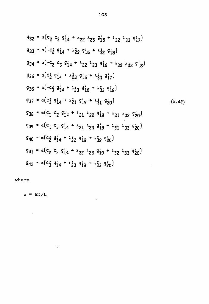
· 105
932 ’ 9192 92 914 * *22 *22 gis * *22 *22 917)
933 ' 9(‘92 914 * *22 gis * *22 gis)
934 ’ 9(‘92 92 914 * *22 *22 gis * *22 *22 gis)935 ’ 9192 914 * *22 gis * *22 917)
935 “ 9(‘92 914 * *22 916 * *22 gis)
937 ‘ 9(91 914 * *21 gis * *21 920) 15.421938 ’ 9(91 92 914 * *21 *22 gis * *21 *22 920)939 ‘ 9191 92 gi4 * *21 *22 gis * *21 *33 920)
940 · 9192 912 + *22 91s + *22 920)941 “ 9(92 92 914 * *22 *22 gis * *22 *22 920)
942 ’ 9192 914 * *22 gis * *22 920) ·
where
a = EI/L

Chapter VI
SOLUTION ALGORITHMS
6.1 INTRODUCTION
The response of a nonlinear structure may be solved ap-
proximately for incremental nodal displacements by taking a
series of linear steps. Many different solution schemes
have been proposed to solve the nonlinear equilibrium Eqs.
(2.55) and (2.104). Here the numerical solutions are ob-
tained by applying either the Newton-Raphson method or the
modified Riks/Wempner method to the nonlinear equilibrium
equation. The former, efficient for low convergence toler-
ance [16], is popularly used to trace nonlinear prebuckling
paths of structures; however, it cannot trace the response
beyond the limit point. The latter has been especially pro-
posed to overcome this problem and can trace nonlinear post
critical response [27]. Both solution techniques are de-
scribed briefly in this chapter.
106
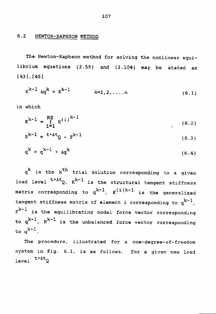
107
6.2 NEWTON-RAPHSON METHOD
The Newton-Raphson method for solving the nonlinear equi-
librium equations (2.55) and (2.104) may be stated as
[43l,[45l
Kknl Aqk=
Rk—lk=l,2,....n (6.1)
in which
_ NE . k-1Kk 1 = _x 1<(1) (6.2)1:1 •
Rk-1 = t+AtQ _ Fk-1 (6.3)
k k—1 kq = q + Aq (6-4)
k . th . . . .q 1S the k trial solution corresponding to a given
load level t+AtQ, Kk-1 is the structural tangent stiffness
matrix corresponding to qk-1, K(i)k·1 is the generalized
tangent stiffness matrix of element i corresponding toqk—l,
Fk—lis the equilibrating nodal force vector corresponding
to qk_l,Rk_l
is the unbalanced force vector corresponding
toThe procedure, illustrated for a one-degree-of-freedom
system in Fig. 6.1, is as follows. For a given new load
level t+AtQ
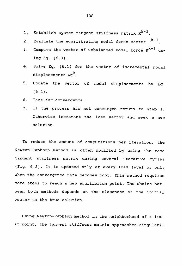
108
1. Establish system tangent stiffness matrix Kk—l.
2. Evaluate the equilibrating nodal force vector Fk-1.
3. Compute the vector of unbalanced nodal forceRk—l
us-
ing Eq. (6.3).
4. Solve Eq. (6.1) for the vector of incremental nodal
displacements Aqk.
5. Update the vector of nodal displacements by Eq.
(6.4).
6. Test for convergence.
7. If the process has not converged return to step 1.
Otherwise increment the load vector and seek: a new
solution.
To reduce the amount of computations per iteration, the
Newton-Raphson method is often modified by using the same
tangent stiffness matrix during several iterative cycles
(Fig. 6.2). It is updated only at every load level or only
when the convergence rate becomes poor. This method requires
more steps to reach a new equilibrium point. The choice bet-
ween both methods depends on the closeness of the initial
vector to the true solution.
Using Newton-Raphson method in the neighborhood of a lim-
it point, the tangent stiffness matrix approaches singulari-
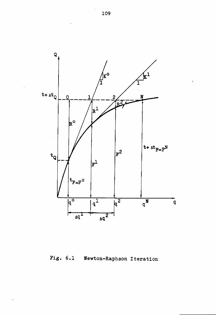
l109
‘ Q
Ko An:·1 1
t+AtQ -0---.-Ä ----2 __ N2'
111/I'
1:+ AtF=FNtQ —
1 2 N|<1° Ia Ia q q^‘1
M12 '
Fig. 6.1 Newton-Raphson Iteration
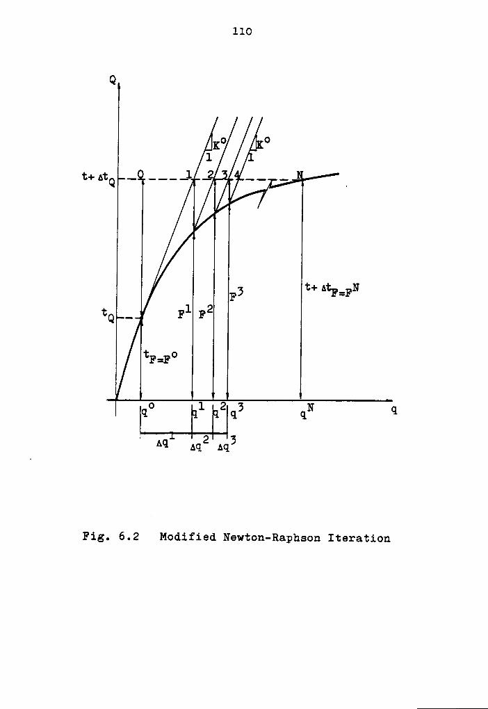
110
Q
lv1
• ]_·
_
F3 t+ ßtF=FN
1tq _ F
tF=F°l 2 N[¤°
ttlqß q q
^q M12 AQ}
Fig. 6.2 Modified Newton-Raphsou Iteratiou

lll
ty resulting in an increasing number of iterations and
smaller and smaller load step; finally the solution diverg-
es. Therefore, it cannot trace the response beyond the lim-
it point. To solve this problem, the modified Riks/Wempner
method is recommended [27].
6.3 MODIFIED RIKSÄWEMPNER METHOD
The theoretical development was recently summarized in
reference [27]. Therefore, details are omitted here. The ba-
sic idea of the Riks/Wempner method is to choose a general-
ized arc length to facilitate the procedure of seeking a new
solution [45],[46]. For a given basic load incremental AX1,
the generalized arc legngh AS can be computed from the
constraint equation. Then the iteration path follows a nor-
mal plane to the tangent, and the new equilibrium point will
be the intersection of the normal plane with the equilibrium
path. Iteration along a circle (or sphere in space) will not
be considered here [27],[47]. In this section the notation
of reference [27] is adopted.
The algorithm of the modified Riks/Wempner method is
briefly summarized as follows (Figs. 6.3 and 6.4):
For the First Step
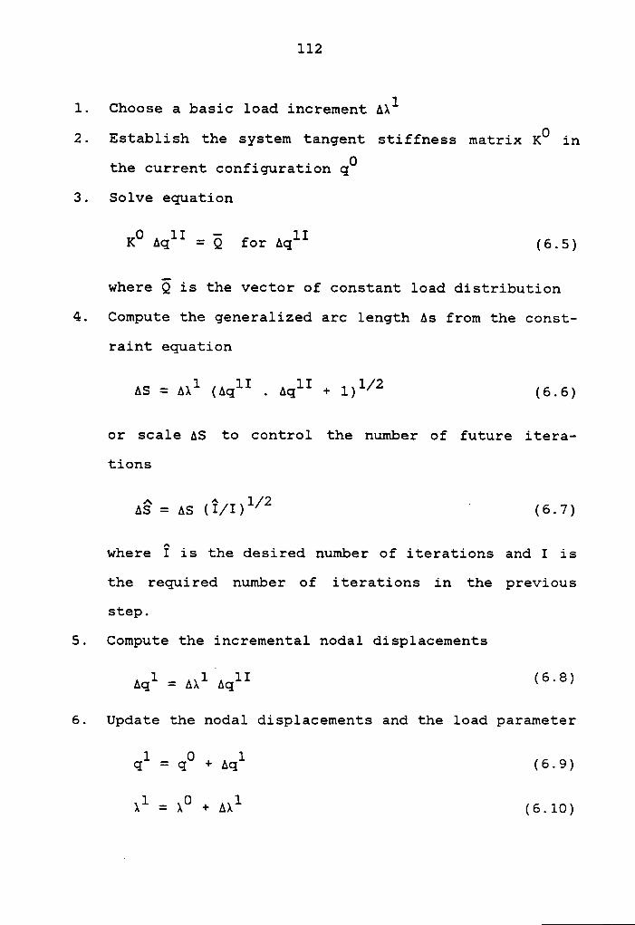
112
1. Choose a basic load increment A11
2. Establish the system tangent stiffness matrix KO in
the current configuration qo
3. Solve equation
KO Aqll = 6 66: AqlI (6.5)
where Ö is the vector of constant load distribution
4. Compute the generalized arc length As from the const-
raint equation
AS = A11 (AqlI . Aqll + 1)l/2 (6.6)
or scale AS to control the number of future itera-
tions
1 2 .A§ = AS (lf/I) / (6-7)
where 1 is the desired number of iterations and I is
the required number of iterations in the previous
step.
5. Compute the incremental nodal displacements
Aql = AÄ1 Aqll (6.8)
6. Update the nodal displacements and the load parameter
ql=
qo+
Aql(6.9)
11=
10 + A11 (6.10)
113
During the kthiteration on normal plane, k=2,3, ....
7. Compute the nodal force vector Fk_l corresponding to
k—1q
8. Update the load vector
Qk'l = )k'l Q (6.11)
9. Compute the unbalanced force vector
Rk-1 = Qk—1 _ Fk-1 (6-12)
10. Update the system tangent stiffness matrixKk_1
if
desirable
kl kll . .11. Solve for Aq and Aq from the two sets of equ1l1-
brium equations
Kkel Aqkl= Ö (6.13)
Kk-1 AqkII= Rk-1 (6-14)
12. Compute the incremental load parameter
Mk = -(Aql. AqkII)/(Aql.AqkI + M1) (6.15)
13. Compute the incremental nodal displacement vector
Aqk = Mk Aqkl + AqkII (6.16)
114
14. Update the nodal displacement vector and the load
parameter
k k-1 kq = q + Aq (6.17)
xk = )k'l + Mk (6.18)
15. Repeat steps 7 to 14 until process has converged
16. Start a new step by returning to step 2.
In conclusion, the modified Riks/Wempner method has been
successfully applied to a variety problems [27],[43].
6.4 CONVERGENCE CRITERIA
The incremental solution at the end of each iteration
should be checked to see whether it has converged within
preset tolerances. Two displacement criteria and one force
criterion are discussed in this section.
Cook [33] adopted the displacement criterion based on the
infinity vector norm:
||Aqk|| qk|| 6 cpmc (6.19)m Q
where Aqk is the maximum incremental displacement, qkis the
maximum total displacement of same type, and CPDC is the
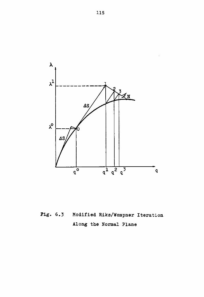
115
Ä
Al ___________ „3Ahn;
AS
AS‘
· 5<1° ql qz q q
Fig. 6.3 Modified Rika/Wempner Iteration
Along the Normal Plane
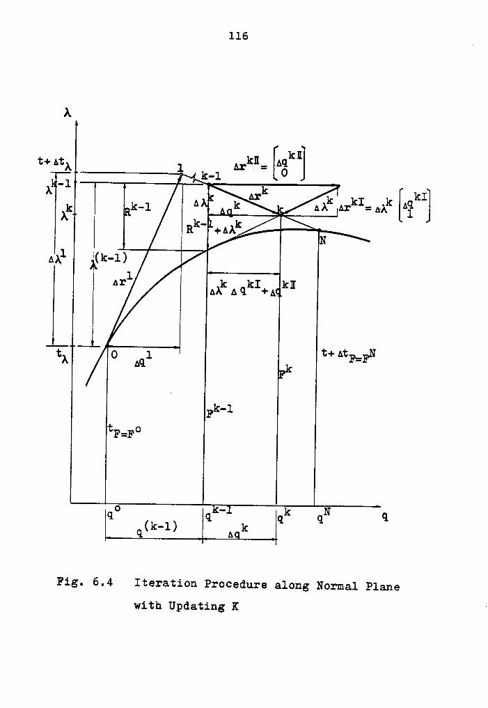
116
A
klk_1 0
A ·kIk ,. Mk ^’kI‘MkÄ
Rk- ÄN
AA; A$k—l)’
1Ar A qkI+A kl
T O 1 t+ At _FNÄ AQ I__ F-
Pk-1
tF=Fo
QO(k 1)
Q-k
Qk QN qq
_A
Fig. 6.4 Iteration Procedure along Normal Plane
with Updating K - °
117
displacement convergence parameter adopted by Cook with the
following range:
-6 -210 S CPDC S 10 (6.20)
Bathe [38],[49] recommends the displacement criterion
based on the Euclidean vector norm:
|| Aqk 2 x qk|| 2 6 c1=·¤B (6.21)where CPDB is the displacement convergence parameter adopted
by Bathe with the value
CPDB = 0.001 (6.22)
A third convergence criterion could be defined as the ra-
tio of the norm of the residual load to the norm of the ori-
ginal load increment [38],[49]:
II "“°^°¤ · EIEEFRIIZ / II‘°‘“^*¤
· )=‘°|I2 6 CPE <¤·23>where CPF is the convergence parameter for the unbalanced
force criterion with a convergence tolerance of 0.1.
Chapter VII
SAMPLE ANALYSIS
7.1 INTRODUCTION
The U.L formulation described in Chapter 2 has been em-
ployed in the computer program. Four examples were investi-
gated in this study and comparisons between the finite ele-
ment model and the beam-column model were made. All of the
test structures were treated as space frames and analyzed by
the modified Riks/Wempner method.
7.2 EXAMPLE 1: WILLIAMS' TOGGLE FRAME
Williams [24], Wood and Zienkiewicz [20], and Papadrakak-
is [21] investigated this problem. Fig. 7.1 shows the co-
nfiguration and properties.
The finite element solution is presented in Fig. 7.2 to
compare the effects of mesh refinement. One, four, six, and
twelve elements per member are used . The responses of the
different meshes are in close agreement up to near the limit
point. Beyond this region,the single element is too stiff,
but four elements are adequate for modeling the behavior of
the toggle frame.
118 V
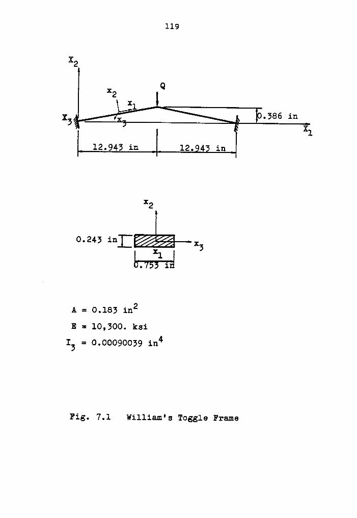
119
X2
QX2 IX1.586 inX6
X112.945 in 12. in
X2
9-29 i¤]i@—.,O 1IVv6x6L;I
A = 0.185 1112E = 10,500. 1191
13 = 0.00090059 IIJ14
Fig. 7.1 Wil1iam's Toggle Frame
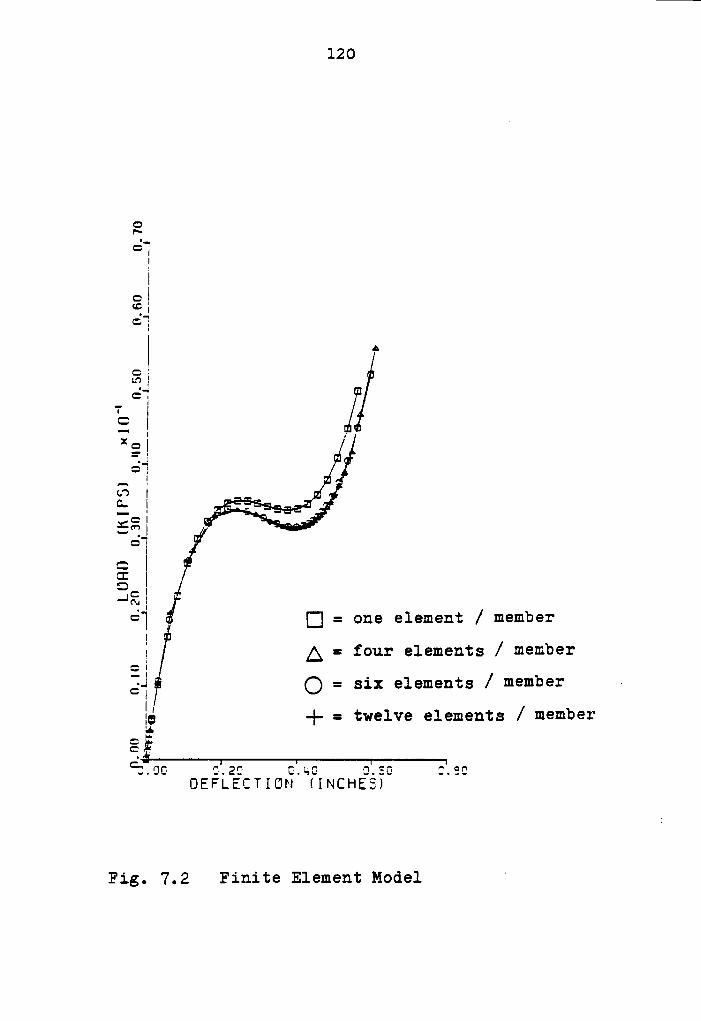
120
caf~
*57II
cI‘°I*57
I•
Qi¤=I
*7I5 IX2! II
-57cn Io. I _
EFIé”Ié Iis: I*57
:3),[:] = one element / member
IA = fOuI' elements / ¤1€!!1b€I‘
:I
Q = six elements / mémbér ~Iä
-|- = twelve elements / member
25··
c‘;‘.0G CJ.2'3 CAO SMEG C.9CÜEFLECTIÜN IINCHEE)
Fig. 7.2 Finite Element Model‘
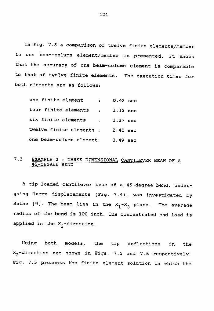
121
In Fig. 7.3 a comparison of twelve finite elements/member
to one beam-column element/member is presented. It shows
that the accuracy of one beam-column element is comparable
to that of twelve finite elements. The execution times for
both elements are as follows:
one finite element : 0.43 sec
four finite elements : 1.12 sec
six finite elements : 1.37 sec
twelve finite elements : 2.40 sec
one beam-column element: 0.49 sec
7.3 EXAMPLE 2 : THREE DIMENSIONAL CANTILEVER BEAM QF Q45-DEGREE BEND
A tip loaded cantilever beam of a 45-degree bend, under-
going large displacements (Fig. 7.4), was investigated by
Bathe [9]. The beam lies in the X1-X3 plane. The average
radius of the bend is 100 inch. The concentrated end load is
applied in the X2—direction.
Using both models, the tip deflections in the
X2-direction are shown in Figs. 7.5 and 7.6 respectively.
Fig. 7.5 presents the finite element solution in which the
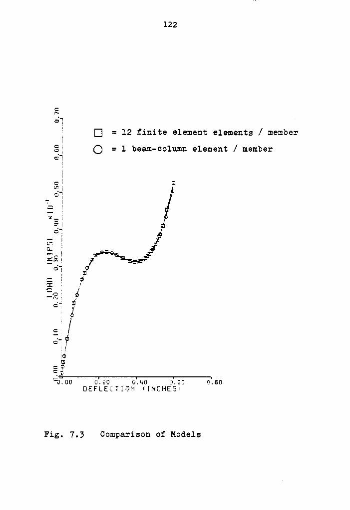
122
Cf*
öl[I] = 12 finite element elements / member
Q = 1 beam·column element / member
°II
cI '*‘Vis='I
E I§-IEis
el
- sigesEr ·’
7:; gg—~e ,6 7*I I
E?I6
m= S?ex:0.00 0.20 0.u0 0.60 0.60
DEFLECTIEIM IINCHESI
Fig. 7.3 Comparison of Models
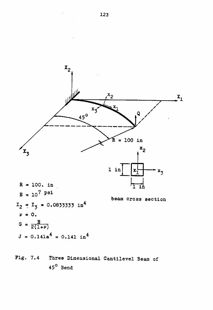
' 123
X2
. X2 X1
X x /1/O 3 ¤ 145
I 1 ·1
R = ].OO illx2X;
l in! g :3
R=lOO. inv I1 ii_ 7 psiE ° 10 beam cross sectionI2 Q I3 = 0.0833333 1114
V =O•
G _ E' 2Z1+v)
J = O.l41a4 = 0.141 1114
Fig. 7.4 Three Dimensional Cantilevel Beam of
45° Bend
124
effects of different mesh refinements are compared; it shows
that two and four elements fail (solution procedure breaks
down), but eight elements are adequate to model the behavior
of the curved beam. Fig. 7.6 presents the beam-column solu-
tion obtained using four and eight elements; it gives simi-
lar results for both meshes. Fig. 7.7 presents a comparison
of four beam-column elements to eight finite elements; the
response predicted by eight finite elements is slightly
stiffer and less accurate than the response predicted by
four beam-column elements.
The result obtained using four beam-column elements is
also compared to the Bathe's solution [9] using eight finite
elements (Fig. 7.8); it can be seen that the beam-column so-
lution produces a similar level of accuracy using a much
coarser mesh. The deflected shapes of the cantilever beam
at various load levels are depicted in Fig. 7.9. The execu-
tion times for both models are as follows:
four elements:
finite element model: 5.66 sec
beam-column model: 7.19 sec
eight elements:
finite element model: 37.27 sec
beam-column model: 37.35 sec
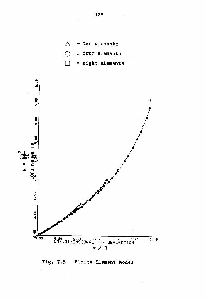
125 ·
A = two elementsl
Q = four elements .
Q = eight elements
c:•6
c .
3‘=‘..
S _ ··:5
IL: ..u.1Nälh, IQ .¤ E2 ..u in
MAd ··E}?„_~__ ..
2c
.-Vit"es ,··—ci g '
ä| Ä u·
71.00 0.08 0.16 0.24 0.32 0.40 0.48NUN—ÜIMENSIÜNF%L TIP ÜEFLECTIÜNv / R
Fig. 7.5 Finite Element Model
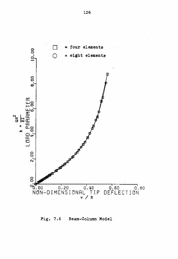
126
Ou
E] = four elements -¤ . .C; Q = eight elements
Il
:1Q
"I
LLJO ‘+-9U-'=¤ „
N é rl
Ü IE ¤Z ‘·
·· go .7I]ä=* ·.
Ü 0.1 _ UM
o.,2,}
O 'Jai _g „·—
0.20 0.40 0.60 0.80NON—D I MENS I ÜNQL T I P DEFLECT I 0N
v / R
Fig. 7.6 Bee,m—Co1umn Model
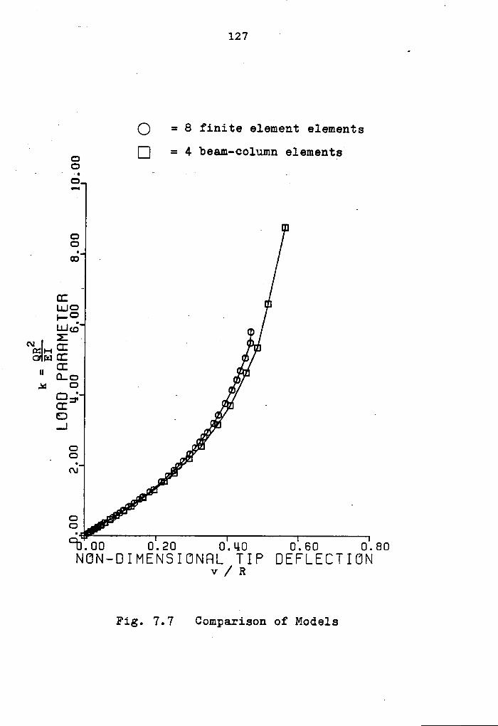
H u127
‘Q = 8 finite element elements
‘Q Ü = 4 beam·column elements
5 . . 6* .1 1 1 .Q
Q_ II
Q
‘
LUG II1-cf · · -U-ko „
Öl ä~ · Hu
u E "un,54 O . ÄC32 ·
Hä 1„¢..1„;‘·
Q $:2;,. ¤ ,,3
C ‘ ;·'
Q000 0.20 0.40 0.60 0.80NON—0IMENSION8L TIP DEFLECTIÜN
v / R
Fig. 7.7 Comparison of Models
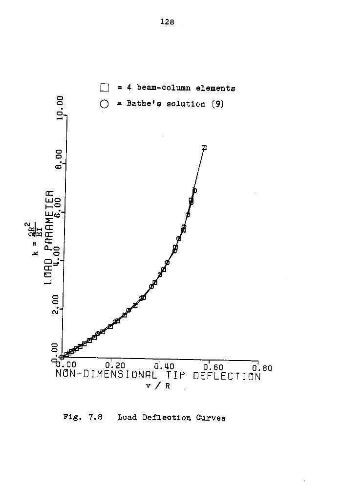
128
I:] = 4 beam—column elementsQ = Bathe's solution [9]
Ilc¤6
T.•—‘=3T28 "N cr: I';gk}: „
II G:1.¤ ca
EJ '·.1 U¤
O HczG;r/Qllb
·;ä.ä‘äO
ij-‘
°0.00 0.20 0.40 0.60 0.80NON—0IMEN‘5ION8L TIP DEFLECTIONv /
RFig.7.8 Load Deflection Curves

129
X2 (inch)
6OO
Q=577.04lb(66.4) 52..39 _1 (600*
501
40 1 0:260.1610(69.6) 38.57 —--__1 1
(600.)30 1
‘I 11 1120 D.S. 1 1I |
lO { {DOSO: I
20• O• O•/ I O•/ O• O;
/ 1 / // X1
___________.. -1/1 // /
20. Ix Q=.<Q'·°—————————————————J 1/(0.)9 —-——————-————————————
X6(inch)
( ) = Bathe¥s results [9]
Fig. 7.9 Deflected Shapes of a 45O Circular Bendusing the Beam·C0lumn Model
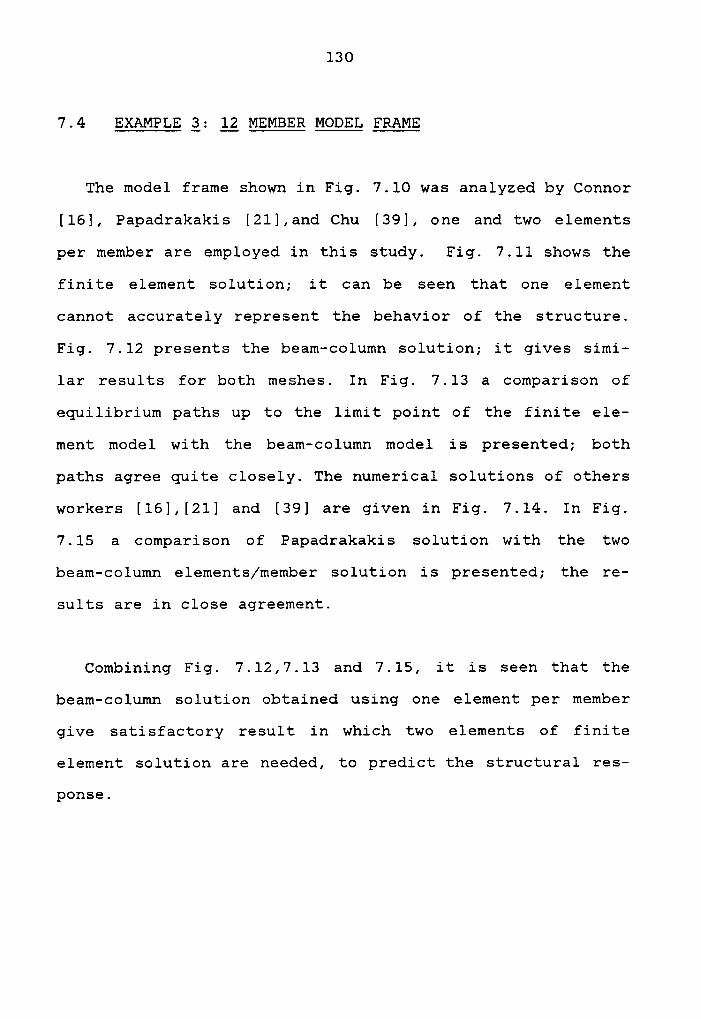
130
7.4 EXAMPLE 3: 12 MEMBER MQQEQ FRQME
The model frame shown in Fig. 7.10 was analyzed by Connor
[16], Papadrakakis [21],and Chu [39], one and two elements
per member are employed in this study. Fig. 7.11 shows the
finite element solution; it can be seen that one element
cannot accurately represent the behavior of the structure.
Fig. 7.12 presents the beam—column solution; it gives simi-
lar results for both meshes. In Fig. 7.13 a comparison of
equilibrium paths up to the limit point of the finite ele-
ment model with the beam—column model is presented; both
paths agree quite closely. The numerical solutions of others
workers [16],[21] and [39] are given in Fig. 7.14. In Fig.
7.15 a comparison of Papadrakakis solution waith the two
beam-column elements/member solution is presented; the re-
sults are in close agreement.
Combining Fig. 7.12,7.13 and 7.15, it is seen that the
beam-column solution obtained using one element per member
give satisfactory result in which two elements of finite
element solution are needed, to predict the structural res-
ponse.
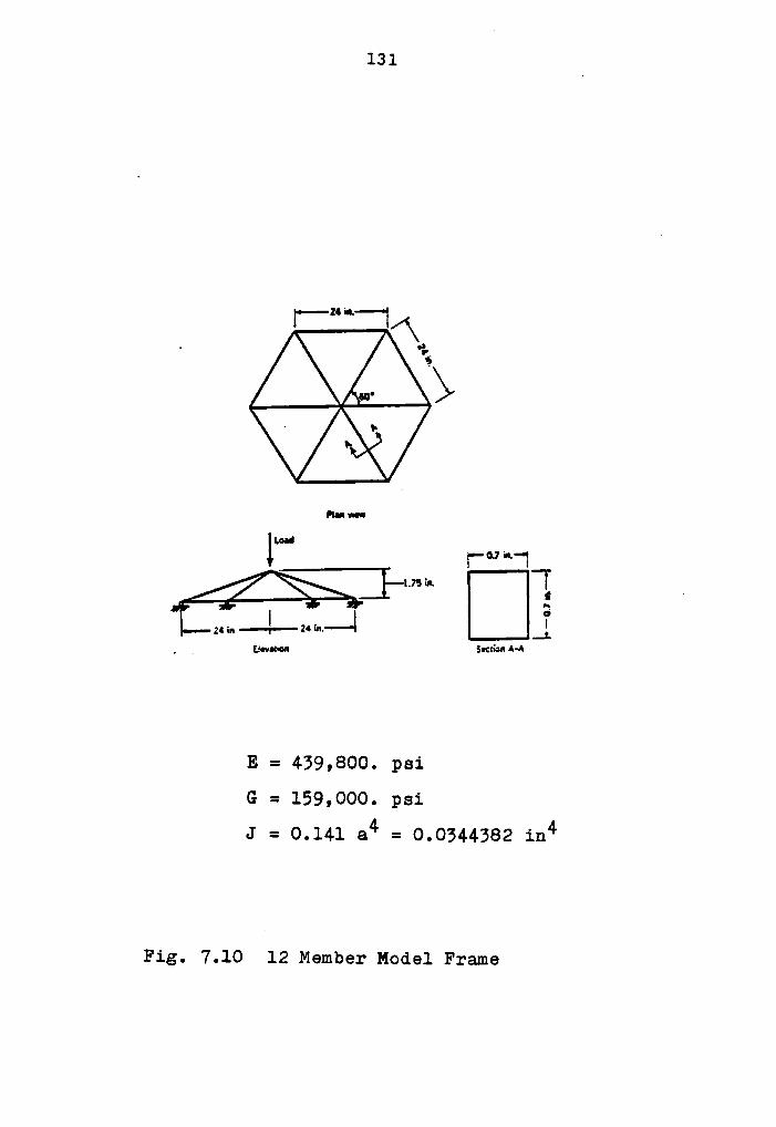
131
l•——z•a•.——~|
’>
H•nv•••
luxV-0.7in.·•7
· PLBM. -1-lE
z•¤••.l·!····•Z"^·“*\gmgmn S•¢xionA·A
E = 439,800. psiG = 159,000. psiJ = 0.141 a4 = 0.0344382 i¤‘*
Fig. 7.10 12 Member Medel Frame
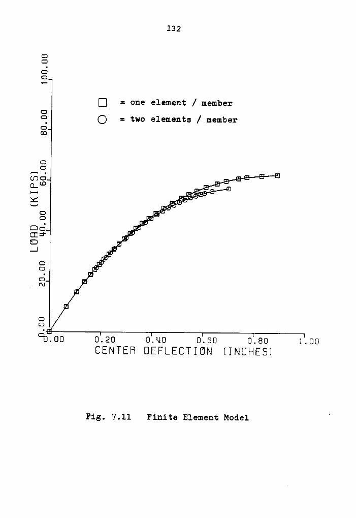
132
CJO
6O
E] = one element / membergi
Q = two elements / member3
OCJ’—‘' .. 3 LI(DO _, : = °0—(-D ._ SDA
9•—• ..;6é=“ ‘K xi: ‘
Q ww:16 .-4*CE=*' „„’*‘Ü *4
—
.1D
gi?C) -2*6 „ "
_ Cu
c>CJ Q00.00 0.20 0.L10 0.60 0.60 1.00
CENTER 0EFI.ECT I 0N (INCHE6]
Fig. 7.11 Finite Element Model”
133
OQ6O
g Ü = O!16 €1€m6¤.‘12 / m8I!1‘b81‘
gg Q = two elements / member
6 .UÜO¤_¢DQ'.
:1.-:;:2
O ,4;.,;-O
„ ‘*'E „,".1 Ä_._'·
G •;’
6 ,_"N
czO
Q0.00 0.20 0.40 0.60 0.80CENTER DEFLECTIÜN IINCHESJ
Fig. 7.12 Beam-Columu Model
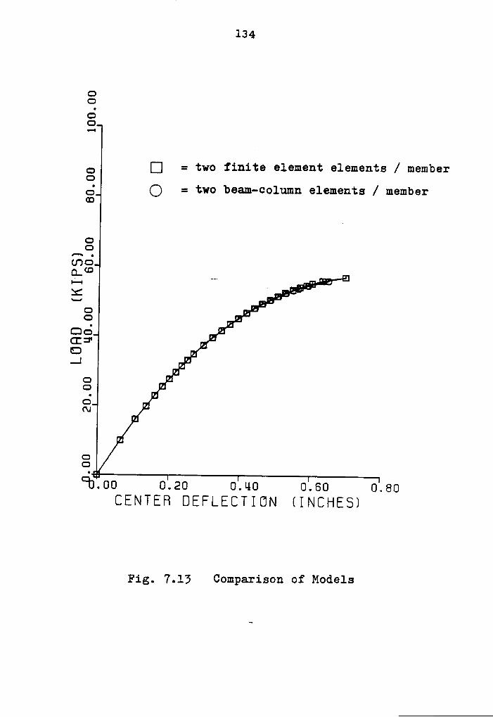
134
QC1
:5Q
5 Q = two finite element elements / memberQ
5 Q = two beam-column elements / memberQ
OO
cm;-SEm -„ =
ca ,*2Q uu
:::3 _ ·»CE=*' ,„
‘
E I4
..1 ,"·
c> _'·~G
' "cg ,_ ’C\.1
QCJ
Q000 0.205 0.110 0.60 0.60CENTER DEFLECTIÜN (INCHE61
Fig. 7.13 Comparison of Models
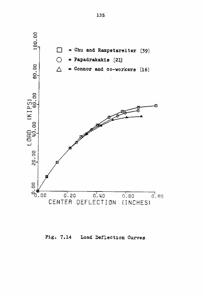
135
GO
si•·*[:| = Chu and Rampatsraitar [39]
Q = Papadrakakis [21]
A == Connor and co-workors [16]6G3
OO
=“
.-. =„ “
0CZ 6;/A
DoCE?u/
6: _„/...1 Il
’”_
caé 6<\1
OCJ
C0.00 0.20 0.LL0 0.60 0.80CENTER ÜEFLECTIUN IINCHESI
Fig. 7.14 Load Deflection Curves
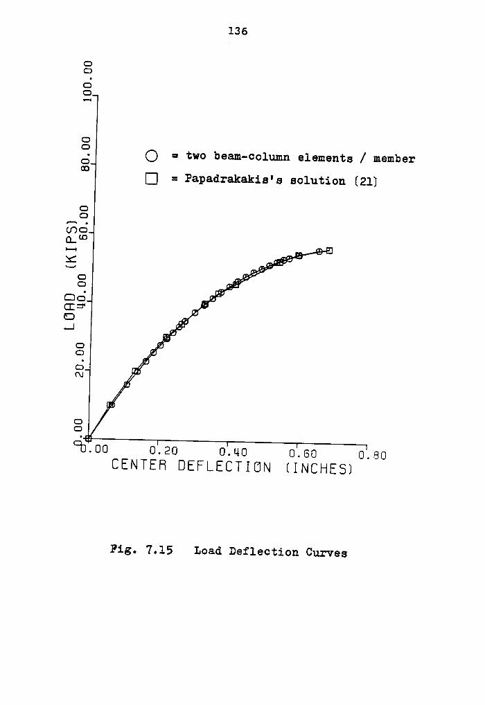
136
6Q
8C; Q = two beam-column elements / memberQ
[Z] = Papad1·akakis's solution [21]
QG
<.o6
QAva},
CJ Ü-?Q6Ü
.·a.I Ä'?
6C)7,*
O nft’\J/¤l
/!«,n
C:ca
0000 0.20 0.40 0.60 0.80CENTER 0EF|.ECTION (INCHESJ
Fig. 7.15 Load Deflection Curves

137
Employing two elements per member, the buckling load ob-
tained by the beam-column model is 56.14 lb and by the fi-
nite element model is 57.24 lb. The execution time for both
models are as followsz
one element:
finite element model: 10.55 sec
beam-column model: 14.55 sec
two elements:
finite element model: 71.53 sec
beam-column model: 75.59 sec
7.5 EXAMPLE 4: RETICULATED QQMQ
Shallow truss domes were investigated by Holzer
[27],[51], Hangai [52], Paradiso [53]. In. this study a
shallow frame dome designed in accordance with the Specifi-
cation of the Aluminum Association [54] is considered. The
geometry* of the reticulated frame dome is <given in. Fig.
7.16. The dome is subjected to a single vertical load at the
center.
Fig. 7.17 presents the finite element solution obtained
using one and two elements per member; it is seen that sin-
gle element is inadequate to model the structural behavior.
138
Fig. 7.18 presents the beam-column solution obtained using
one and two elements per member; similar results for both
meshes are obtained. Fig. 7.19 presents a comparison of two
finite elements to one beam-column element; it shows again
that fewer elements in the beam column model are often need-
ed than in the finite element model for satisfactory accura-
cy.
In addition Fig. 7.19 shows a comparison of two extreme
cases, the shallow truss dome, considered by Uliana [55],
with the present frame dome, is presented; it shows that the
behavior of the frame dome remains linear when the truss
dome reaches the limit point due to a central, concentrated
load. Clearly, the frame dome is much stronger than the
truss dome. The execution time for both models are given as
A
follows:
one element:
finite element model: 52.71 sec
beam—column model: 60.53 sec
two elements:
finite element model: 339.24 sec
beam-column model: 459.41 sec
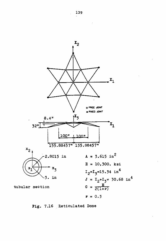
„ 139
12
.A_A_ X.
QFREE •ß|NT
QFIXED MMT
_6.4··X
l55.88457" l55.8845'7"2 1
2.8015 in A = 3.615 in2Q A&\ E = 10,300. 1:61
x‘l 3, 12.1;:16.64 iz143· 1** .1 = I2+I3= 30.68 in4
tubular: section G = E-(Tlßjy
V = O.3
Fig. 7.16 _Reticulated Dome
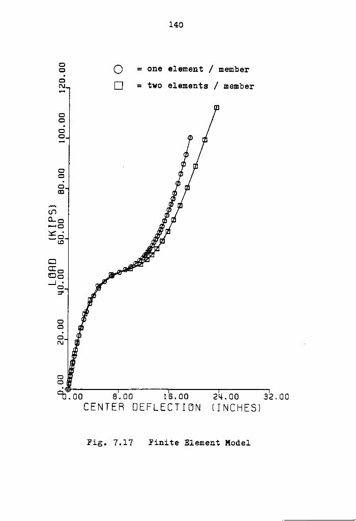
140
Q = one element / member
E] = two elements / member
GQ
ciE n N
> 0
0G
H® n
HQ-Q u U
•—•Qco ,;· *.;€=!".‘=¤"
uyfasuC.:
__·: 4og ‘
.1 ·,..’·
G .·;=• ,/
rf·.I
o "_uu
f\.I 75 ·
·=> é'Ocboo 8.00 18.00 2*4.00 32.00
CENTER ÜEELECT I ÜN (INCHES1
Fig. 7. 17 Finite Element Model
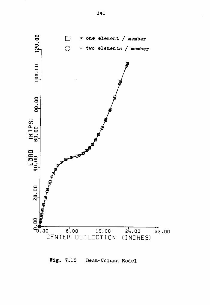
141 A
S E = one element / member
Q = two elements / member
nQ UD
6Il
Q ÜQ
vr1}
¤—cInM
LD "
caä ,. ·=”’
···lé 1;=• O1IA
O?QG J.‘
6 ..(\_| $1
ca X
Gcmoo 8.00 16.00 2*-1.00 32.00CENTER 0EELECTION (INCHE5)
Fig. 7.18 Beam·Column Model
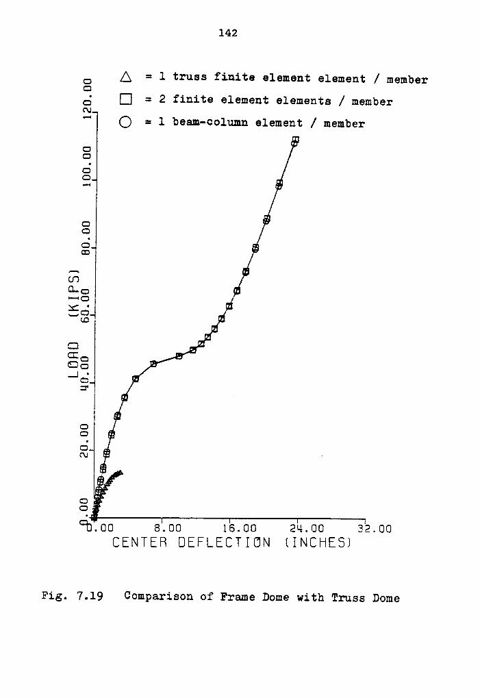
142
Q Ä = l truss finite element element / memberQ6 E] = 2 finite element elements / memberN"‘
Q = 1 beam-column element / member
ClO
6D
GO
6oo
G30-::
In
:.0 '*
Q: 2cg ·=,_
=" .
J!O E:6}N
nl
C3CJ
Q0.00 8.00 18.00 2*4.00 32.00CENTER ÜEFLECTIÜN KINCHEST
Fig. 7.19 Comparison of Frame Dome with Truss Dome
Chapter VIII
PROGRAM DEVELOPMENT
8.1 INTRODUCTION
The program developed by Butler [29], for the geometri-
cally nonlinear static analysis of plane frames, has been
modified and extended to the GNSSF (Geometrically Nonlinear
Static Analysis of Space Frames) program using U.L. formula-
tion as in appendix F. The modified program has the capabil-
ity to analyze space frames with arbitrary large displace-
ment. It is restricted to continuous, elastic structures,
i.e., only geometrical nonlinearity is considered.
The GNSSF computer program is written in the WATFIV ver-
sion of FORTRAN code having the following options:
1. Newton-Raphson method or modified Riks/Wempner method
2. beam-column model or finite element model
Subroutines FORCES and STIFF can be approached by using
either the beam-column model or the finite element model.
Subroutines FACTOR, REDUCE, and BACSUB, adapted from Bathe
[38] and Subroutines SOLVE, TEST, DISPLC, DISPLB, UNBALF,
UPDATE, DOTPRD, adapted from Butler [29], will not be de-
scribed here.
143
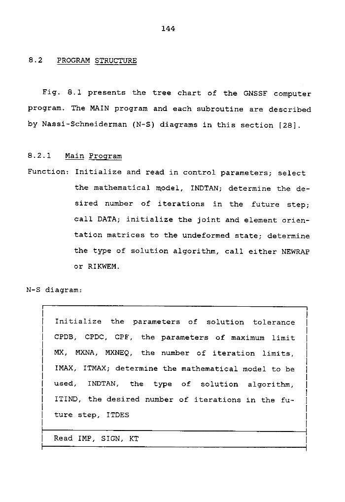
144
8.2 PROGRAM STRUCTURE
Fig. 8.1 presents the tree chart of the GNSSF computer
program. The MAIN program and each subroutine are described
by Nassi—Schneiderman (N-S) diagrams in this section [28].
8.2.1 Mglg Program
Function: Initialize and read in control parameters; select
the mathematical model, INDTAN; determine the de-
sired. number of iterations in the future step;
call DATA; initialize the joint and element orien-
tation matrices to the undeformed state; determine
the type of solution algorithm, call either NEWRAP
or RIKWEM.
N—S diagram:
I I{ Initialize the parameters of solution tolerance |
{ CPDB, CPDC, CPF, the parameters of maximum limit {
{ MX, MXNA, MXNEQ, the number of iteration limits, {
{ IMAX, ITMAX; determine the mathematical model to be {
{ used, INDTAN, the type of solution algorithm, {
{ ITIND, the desired number of iterations in the fu- {
{ ture step, ITDES {I I{ Read IMP, SIGN, KT |
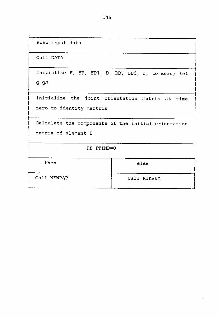
145
I Echo input data II II Call DATA |I II Initialize F, FP, FPI, D, DD, DDO, Z, to zero; let II II Q=QJ II II Initialize the joint orientation matrix at time II II zero to identity martrix II II Calculate the components of the initial orientation II II matrix of element I II I| If 1T1ND=0 |I II then else II II Call NEWRAP ca11 RTKWEM |I I
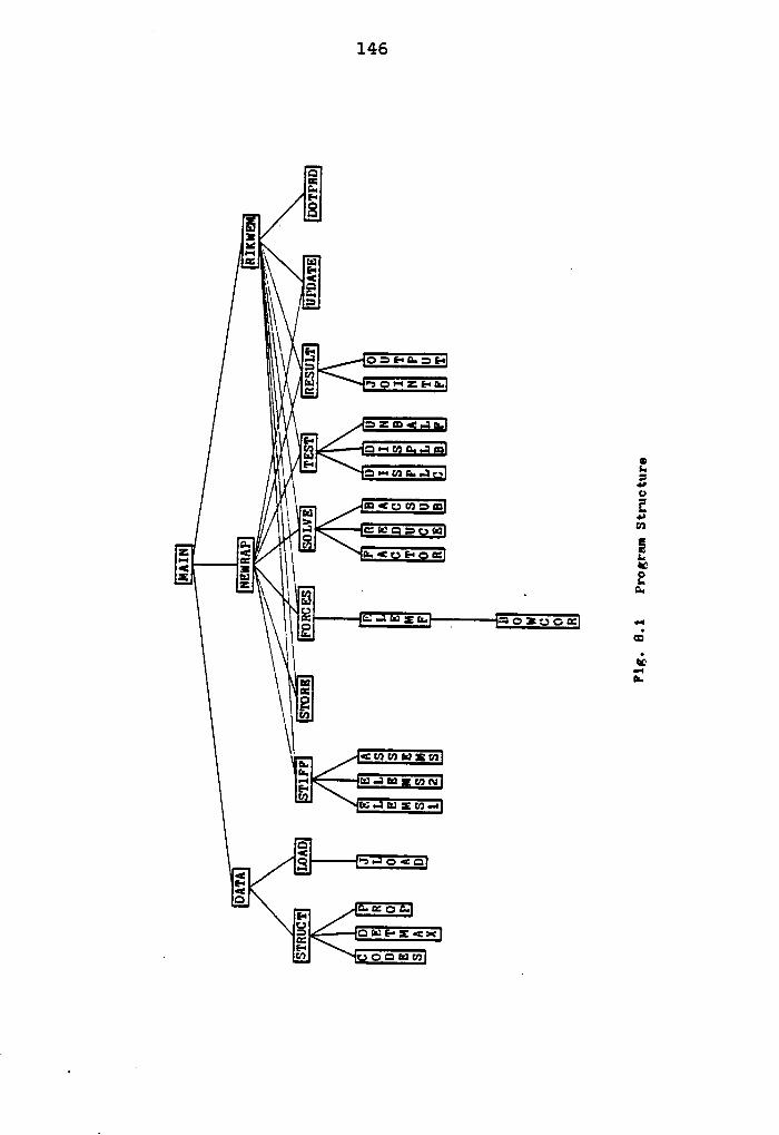
146
ES
aazrxsm
Emaarm '”
Ex\§
‘ aämzzmEumvazm
rzaaz@2:::1:;:1— utßzm
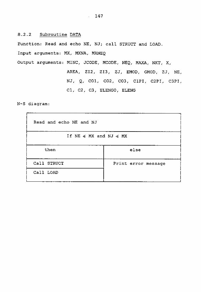
· 147
8.2.2 Subroutine QAQA
Function: Read and echo NE, NJ; call STRUCT and LOAD.
Input arguments: MX, MXNA, MXNEQ
Output arguments: MINC, JCODE, MCODE, NEQ, MAXA, NKT, X,
AREA, ZI2, ZI3, ZJ, EMOD, GMOD, ZJ, NE,
NJ, Q, CO1, CO2, CO3, C1PI, C2PI, C3PI,
C1, C2, C3, ELENGO, ELENG
N-S diagram:
I I| Read and echo NE and NJ II II If NE 6 Mx and NJ 6 Mx II I| then else |I II Call STRUCT Print error message I
I Call LoAD E
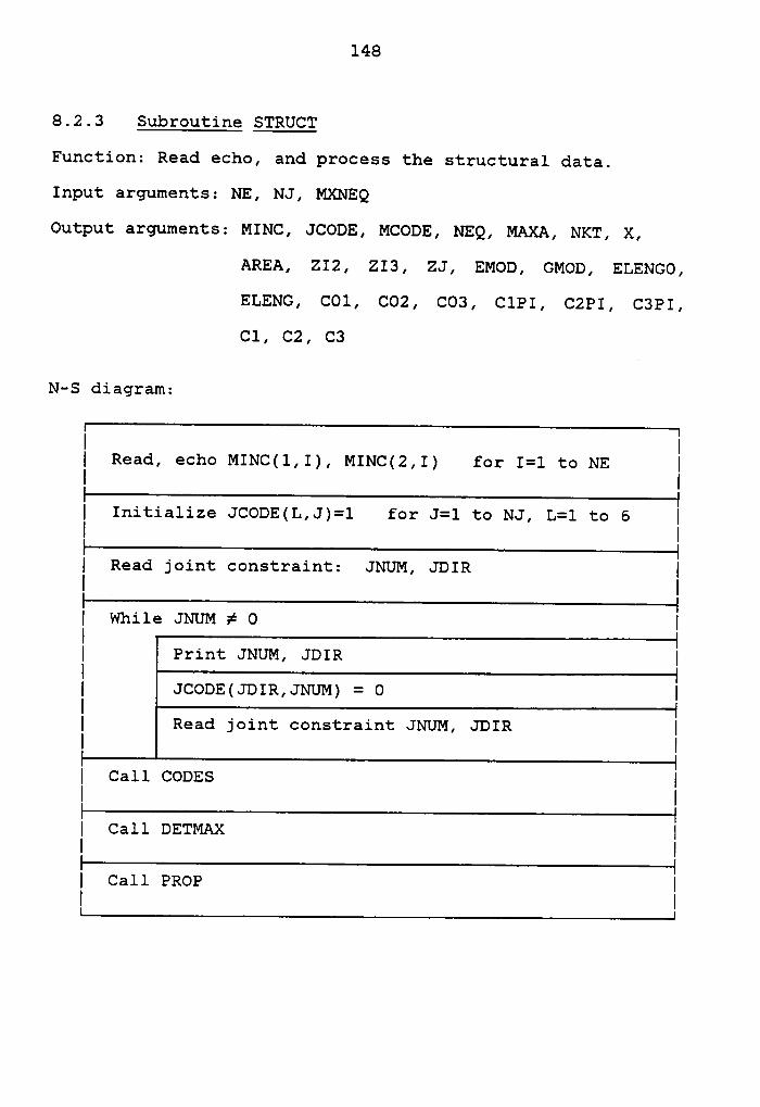
148
8.2.3 Subroutine STRUCT
Function: Read echo, and process the structural data.
Input arguments: NE, NJ, MXNEQ
Output arguments: MINC, JCODE, MCODE, NEQ, MAXA, NKT, X,
AREA, ZI2, ZI3, ZJ, EMOD, GMOD, ELENGO,
ELENG, CO1, CO2, CO3, C1PI, C2PI, C3PI,
Cl, C2, C3
N-S diagram:
I II Read, echo MINC(l,I), MINC(2,I) for I=l to NE |I II Initialize JCODE(L,J)=1 for J=1 to NJ, L=l to 6 II II Read joint constraint: JNUM, JDIR II II while JNUM ¢ 0 III Print JNUM, JDIR II| JCODE(JDIR,JNUM) = 0 |II Read joint constraint JNUM, JDIR II II Call comzs II II Call DETMAX
II
I Call PaopII
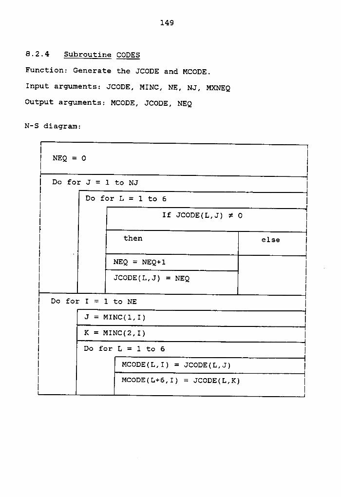
149
8.2.4 Subroutine QQQE§
Function: Generate the JCODE and MCODE.
Input arguments: JCODE, MINC, NE, NJ, MXNEQ
Output arguments: MCODE, JCODE, NEQ
N-S diagram:
I II NEQ = O II I{ Do for J = 1 to NJ {
{ Do for L = 1 to 6 {{ If JCODE(L,J) ¢ O {{ I{ then else {{ I I| NEQ = NEQ+1 { _{ JCODE(L,J) = NEQ {I I{ Do for I = 1 to NE {{ J = MINC(l,I) |{ K = M1Nc(2,1) |{ Do for L = 1 to 6 {
{ MCODE(L,I) = JCODE(L,J) {
{ MCODE(L+6,I) = JCODE(L,K){
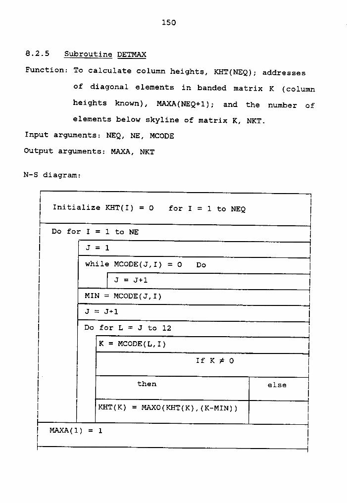
150 ·
8.2.5 Subroutine DETMAX
Function: To calculate column heights, KHT(NEQ); addresses
of diagonal elements in banded matrix K (column
heights known), MAXA(NEQ+1); and the number of
elements below skyline of matrix K, NKT.
Input arguments: NEQ, NE, MCODE
Output arguments: MAXA, NKT
N—S diagram:
I II
Initialize KHT(I) = 0 for I = 1 to NEQI
I Do for I = 1 to NE I
I J = l II while MCODE(J,I) = O Do I
I J=J+1 I
I MIN = MCODE(J,I) I
I J = J+1I
I Do for L = J to 12 I
I K = MCODE(L,I) I
I If K ¢ 0 II II _ .I then else I
I I
IKHT(K) = MAXO(KHT(K),(K—MIN))
I
IMAXA(l) = l
I
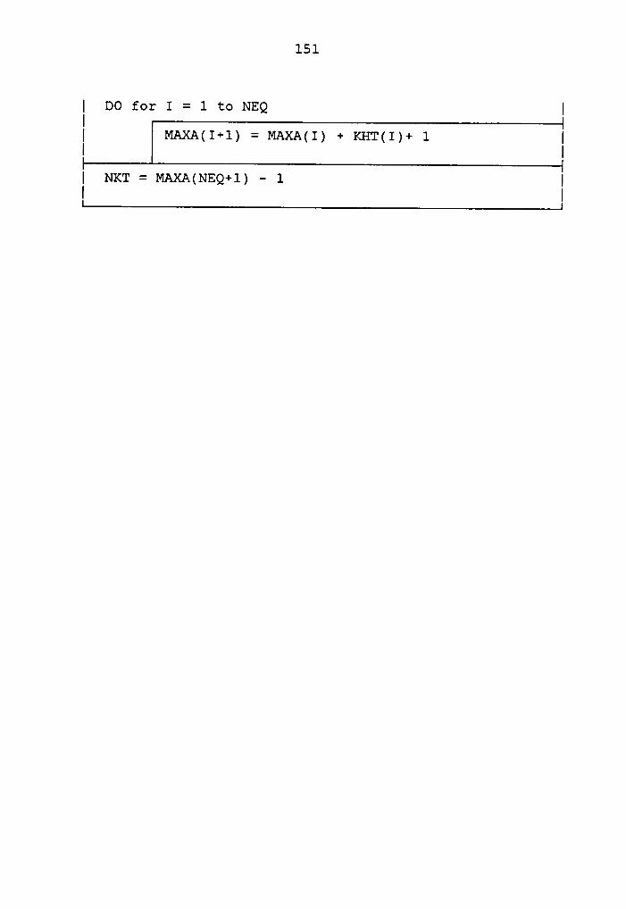
151
| DO for I = 1 to NEQ |I| MAXA(I+l) = MAXA(I) + KHT(I)+ 1 |I I| NKT = MAXA(NEQ+1) - 1 |I IL........_.............................................__J
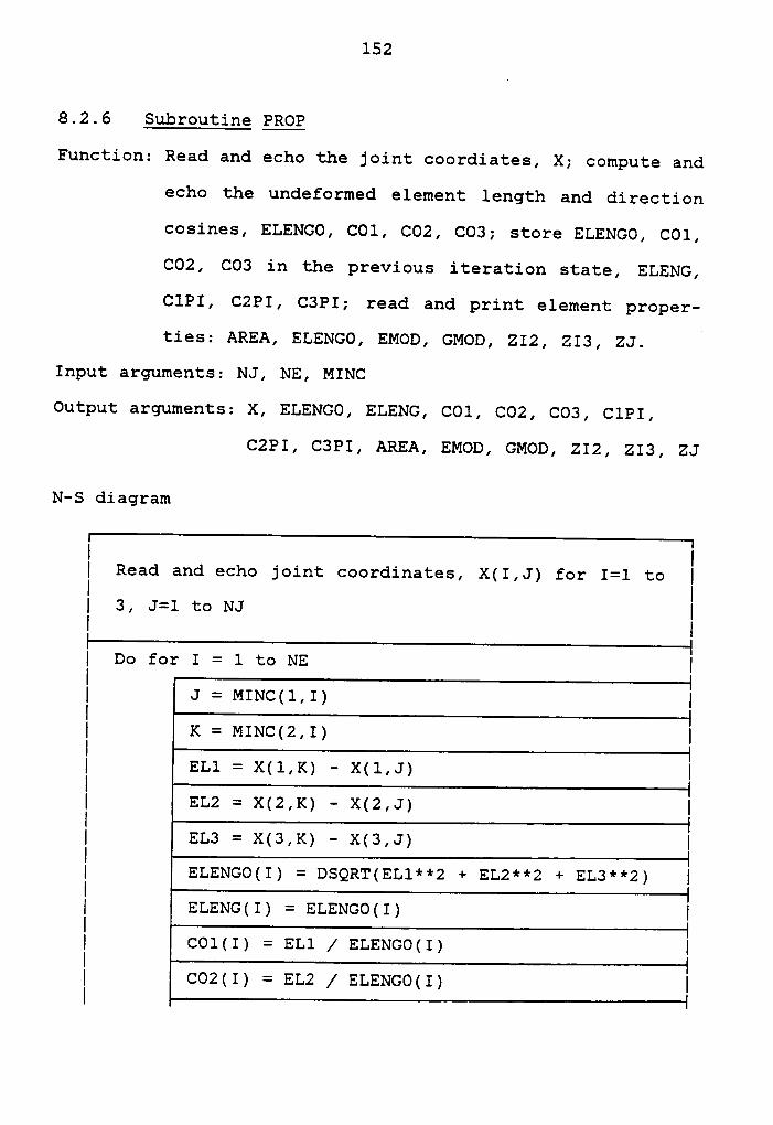
152
8.2.6 Subroutine QRQQ
Function: Read and echo the joint coordiates, X; compute and
echo the undeformed element length and direction
cosines, ELENGO, CO1, CO2, CO3; store ELENGO, CO1,
CO2, CO3 in the previous iteration state, ELENG,
ClPI, C2PI, C3PI; read and print element proper-
ties: AREA, ELENGO, EMOD, GMOD, ZI2, ZI3, ZJ.
Input arguments: NJ, NE, MINC
Output arguments: X, ELENGO, ELENG, CO1, CO2, CO3, ClPI,
CZPI, C3PI, AREA, EMOD, GMOD, ZI2, ZI3, ZJ
N-S diagram
I II Read and echo joint coordinates, X(I,J) for I=l to I
I 3, J=1 to NJII I
I Do for I = 1 to NE II J = M11~1c(1,1) |
I K = MINC(2,I) II EL1 = X(1,K) - X(1,J) II EL2 = X(2,K) — X(2,J) I
I EL3 = X(3,K) - X(3,J) I
I ELENGO(I) = DSQRT(EL1**2 + EL2**2 + EL3**2) I
I ELENG(I) = ELENGO(I) I
I CO1(I) = EL1 / ELENGO(I) I
EL2 / ELENGO(I) I
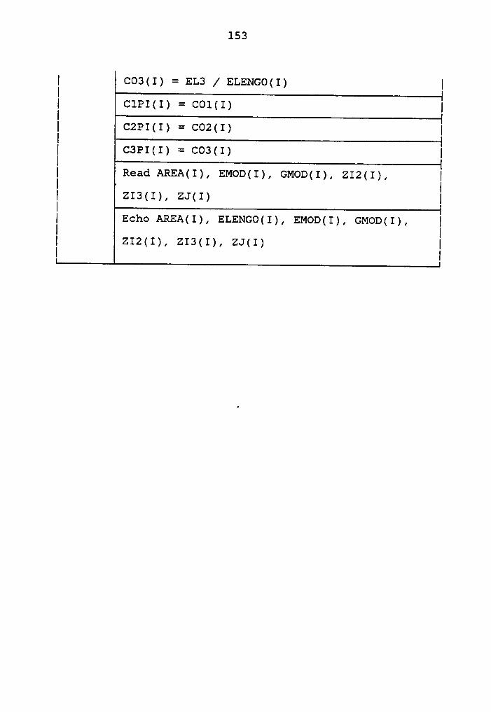
153
I CO3(I) = EL3 / ELENGO(I) I
I ClPI(I) = C01(I) II C2PI(I) = CO2(I) I
I C3PI(I) = CO3(I) I
I Read AREA(I), EMOD(I), GMOD(I), ZI2(I), I
I ZI3(I), ZJ(I) I
I Echo AREA(I), ELENGO(I), EMOD(I), GMOD(I), I
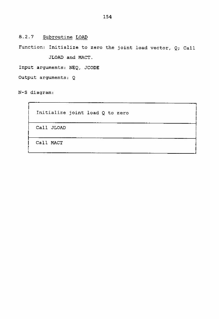
154
8.2.7 Subroutine LOAD
Function: Initialize to zero the joint load vector, Q; Call
JLOAD and MACT.
Input arguments: NEQ, JCODE
Output arguments: Q
N-S diagram:
I I| Initialize joint load Q to zero |I I| Call JLoAD |I I| Call MACT |I Il..........................................................4
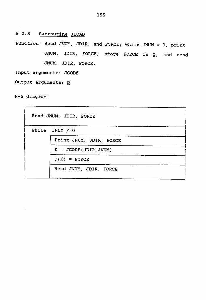
155
8.2.8 Subroutine QQQQQ
Function: Read JNUM, JDIR, and FORCE; while JNUM = O, print
JNUM, JDIR, FORCE; store FORCE in Q, and read
JNUM, JDIR, FORCE.
Input arguments: JCODE
Output arguments: Q
N—S diagram:
I II Read JNUM, JDIR, FORCE II II while JNUM ¢ O I
I Print JNUM, JDIR, FORCE I
I K = JCODE(JDIR,JNUM) I
I Q(K) = EoRcE I
I Read JNUM, JDIR, FORCEI
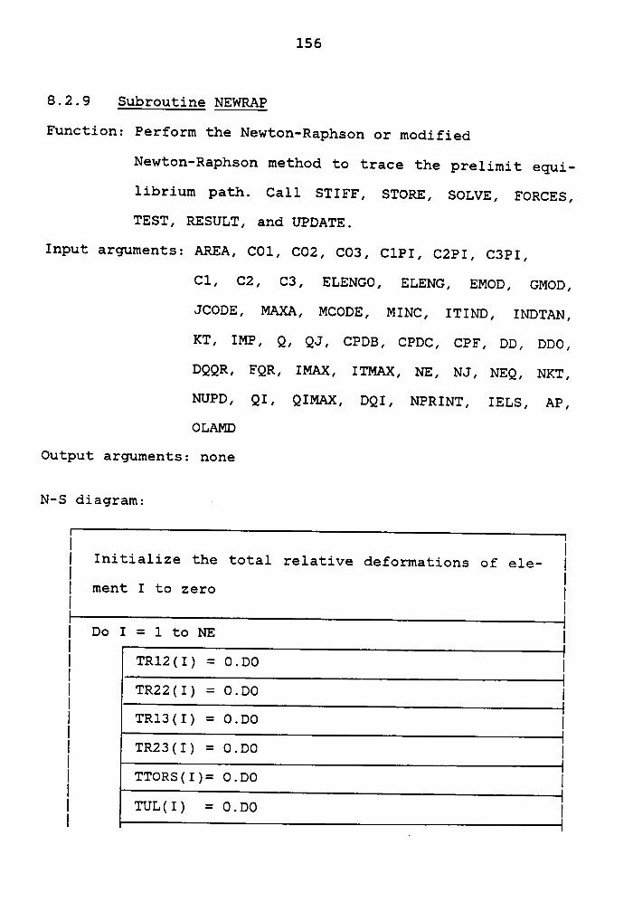
156
8.2.9 Subroutine NEWRAP
Function: Perform the Newton—Raphson or modified
Newton-Raphson method to trace the prelimit equi-
libriunn path. Call STIFF, STORE, SOLVE, FORCES,
TEST, RESULT, and UPDATE.
Input arguments: AREA, COl, CO2, CO3, C1PI, CZPI, C3PI,
C1, C2, C3, ELENGO, ELENG, EMOD, GMOD,
JCODE, MAXA, MCODE, MINC, ITIND, INDTAN,
KT, IMP, Q, QJ, CPDB, CPDC, CPE, DD, DDO,
DQQR, EQR, IMAX, ITMAX, NE, NJ, NEQ, NKT,
NUPD, QI, QIMAX, DQI, NPRINT, IELS, AP,
OLAMD
Output arguments: none
N—S diagram: ·
I II Initialize the total relative deformations of ele- I
I ment I to zero II II Do I = 1 to NE II TRl2(I) = 0.00 II TR22(1) = 0.00 II 1•R13(1) = 0.00 II TR23(I) = 0.00 II TTORS(I)= O.D0 I
ETUL(I) = O.DO I
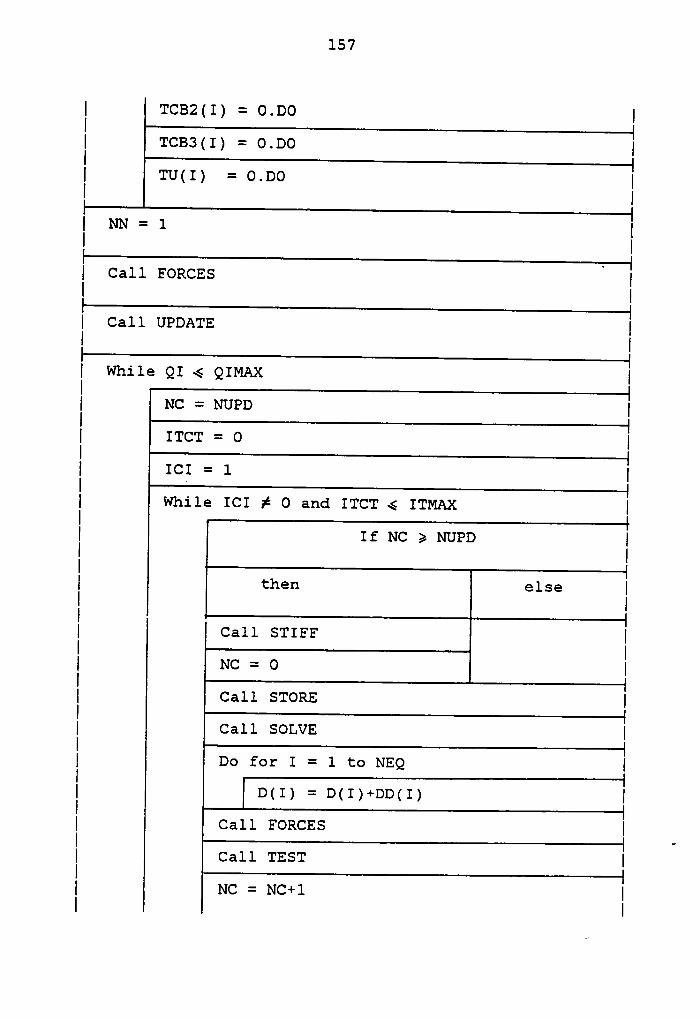
157
I TCB2(I) = 0.DO III TCB3(I) = O.DO III TU(I) = 0.DO II II NN = 1 II II Call FORCES I
II II Call UPDATE II II While QI S QIMAX III NC = NUPD III ITCT = O III ICI = l I—
I While ICI ¢ O and ITCT S ITMAX III If NC 2 NUPD II III then else I
I II Call STIEE II II NC = O III Call STORE III Call SOLVE III Do for I = 1 to NEQ II
I D(1) = D(1)+DD(1) II Call FORCES II„
I Call TEST III NC = NC+1 II I
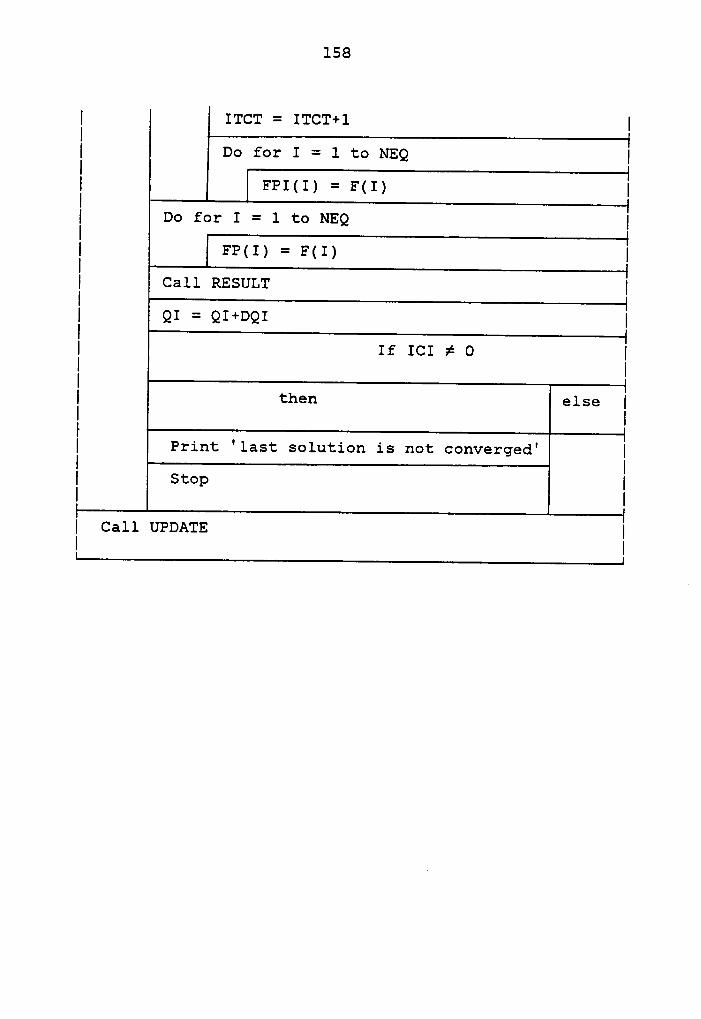
158
I ITCT = ITCT+l III Do for I = 1 to NEQ II
IFPI(I) = F(I) I
I Do for I = 1 to NEQ III
FP(I) = F(I) I
I Call RESULT II
IQI = QI+DQI I
I If ICI ¢ O IIIII then else II II Print 'last solution is not converged' II II Stop II II Call UPDATE II I
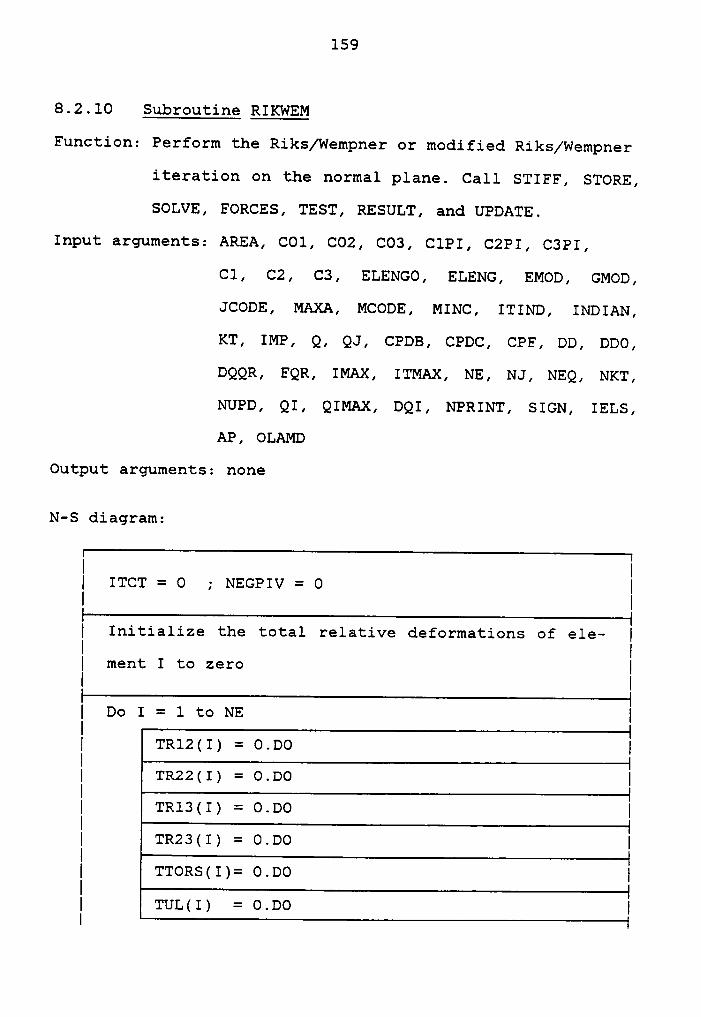
159
8.2.10 Subroutine RIKWEM
Function: Perform the Riks/Wempner or modified Riks/Wempner
iteration on the normal plane. Call STIFF, STORE,
SOLVE, FORCES, TEST, RESULT, and UPDATE.
Input arguments: AREA, C0l, CO2, CO3, ClPI, CZPI, C3PI,
C1, C2, C3, ELENGO, ELENG, EMOD, GMOD,
JCODE, MAXA, MCODE, MINC, ITIND, INDIAN,
KT, IMP, Q, QJ, CPDB, CPDC, CPF, DD, DDO,
DQQR, FQR, IMAX, ITMAX, NE, NJ, NEQ, NKT,
NUPD, QI, QIMAX, DQI, NPRINT, SIGN, IELS,
AP, OLAMD
Output arguments: none
N-S diagram:
I II ITCT = O ; NEGPIV = 0 II II Initialize the total relative deformations of ele—
I
I ment I to zero II Do 1 = 1 to NE II TR12(I) = o.¤o II TR22(1) = 0.Do I
I TR13(1) = o.¤0 II TR23(1) = 0.Do II TTORS(I)= 0.DO I
ITUL(I) = 0.Do I
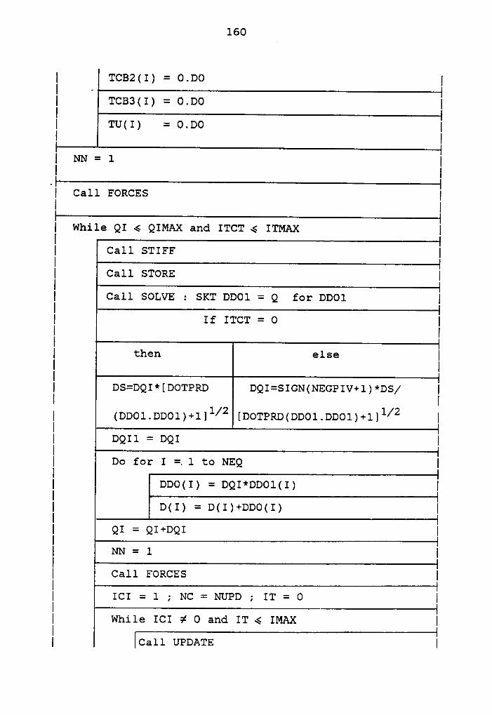
160
I TCB2(I) = 0.DO I
II
TCB3(I) = 0.DO I
I TU(I) = 0.DO II I II NN = 1 II IOI Call FORCES II II While QI 6 QIMAX and ITCT 6 ITMAX I
I Call STIFF II Call STORE II Call SOLVE : SKT DDO1 = Q for DDO1 I
I If ITCT = O II II then else I
I II
DS=DQI*[DOTPRD DQI=SIGN(NEGPIV+1)*DS/
I
I (DDOl.DDO1)+l]l/2 [DOTPRD(DDOl.DDO1)+l]l/2 II DQI1 = DQI I
I Do for I =. 1 to NEQ I
I DDO(I) = DQI*DDO1(I) I
I D(I) = D(I)+DDO(I) I
I Q1 = Q1+DQ1 II NN = 1 I
I Call FORCES I
I ICI=l;NC=NUPD;IT=O I
I While ICI ¢ O and IT 6 IMAX I
I ICall UPDATE I
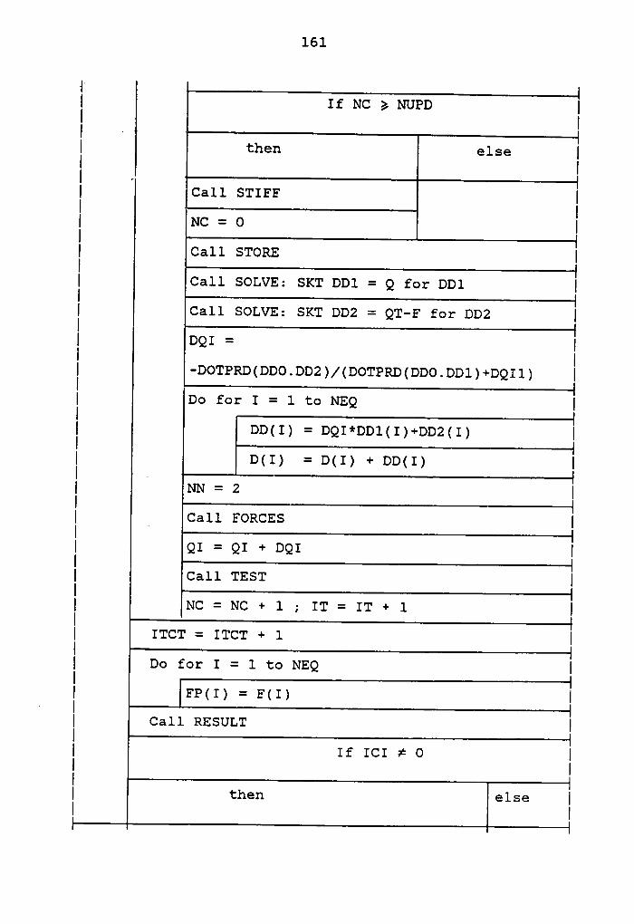
161
I If NC > NUPD II II .I then else I
I II ca11 STIFF II II II Call STORE III Call SOLVE: SKT DDl = Q for DDl III Call SOLVE: SKT DD2 =
Q'I‘—E‘for DD2 II
I DQI ‘II -DOTPRD(DDO.DD2)/(DOTPRD(DDO.DDl)+DQIl) II
I Do fo1:I=ltoNEQ III DD(1) = DQ1*DD1(1)+DD2(1) II
I DII) = D(I) + DD(I) I. ——-——————-———————————————————————+I NN = 2 II ———————————————————————————————%I Call EORcES I—
IQI = QI + DQ1 I
I ca11 TEST III NC = NC + 1 ; IT = IT + 1 III ITCT = ITCT + 1 III Do forI=ltoNEQ III FP(I) = E(1) I· II Call RESULT III If ICI ¢ 0 II III then else II I
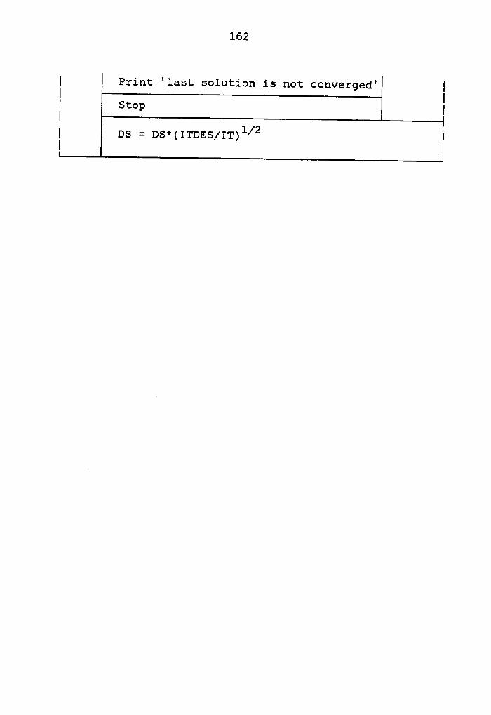
162
| Print 'last solution is not converged' |I I{ I{ DS = DS*(ITDES/IT)1/2
{
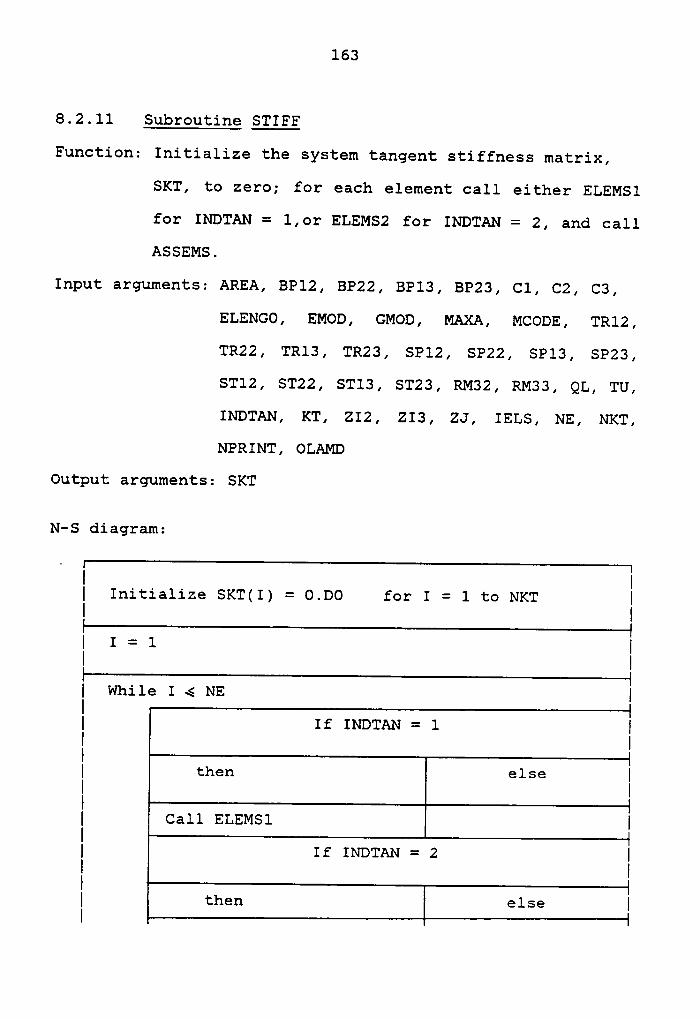
163
8.2.11 Subroutine STIFF
Function: Initialize the system tangent stiffness matrix,
SKT, to zero; for each element call either ELEMS1
for INDTAN = l,or ELEMS2 for INDTAN = 2, and call
ASSEMS.
Input arguments: AREA, BPl2, BP22, BP13, BP23, Cl, C2, C3,
ELENGO, EMOD, GMOD, MAXA, MCODE, TR12,
TR22, TRl3, TR23, SPl2, SP22, SPl3, SP23,
ST12, ST22, STl3, ST23, RM32, RM33, QL, TU,
INDTAN, KT, ZI2, ZI3, ZJ, IELS, NE, NKT,
NPRINT, OLAMD
Output arguments: SKT
N-S diagram:
-II
I Initialize SKT(I) = O.DO for I = 1 to NKT II II I = 1 II II wmie 1 4 NE III If INDTAN = 1 II III then else I
I II Call ELEMSI III If INDTAN = 2 II III then else II
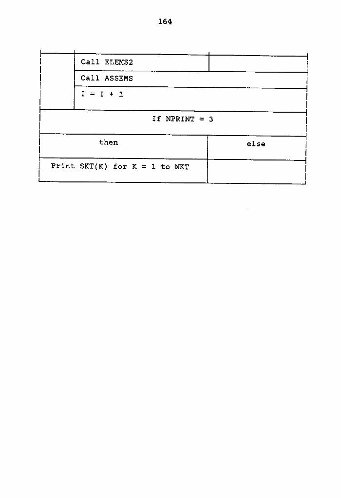
164
I Call ELEMSZ |I| Call ASSEMS |I| I = I + 1 |I I| If NPRINT = 3 |I Il then else |I I 1l Prim: SK'I‘(K) for K = 1 to NKT |I I
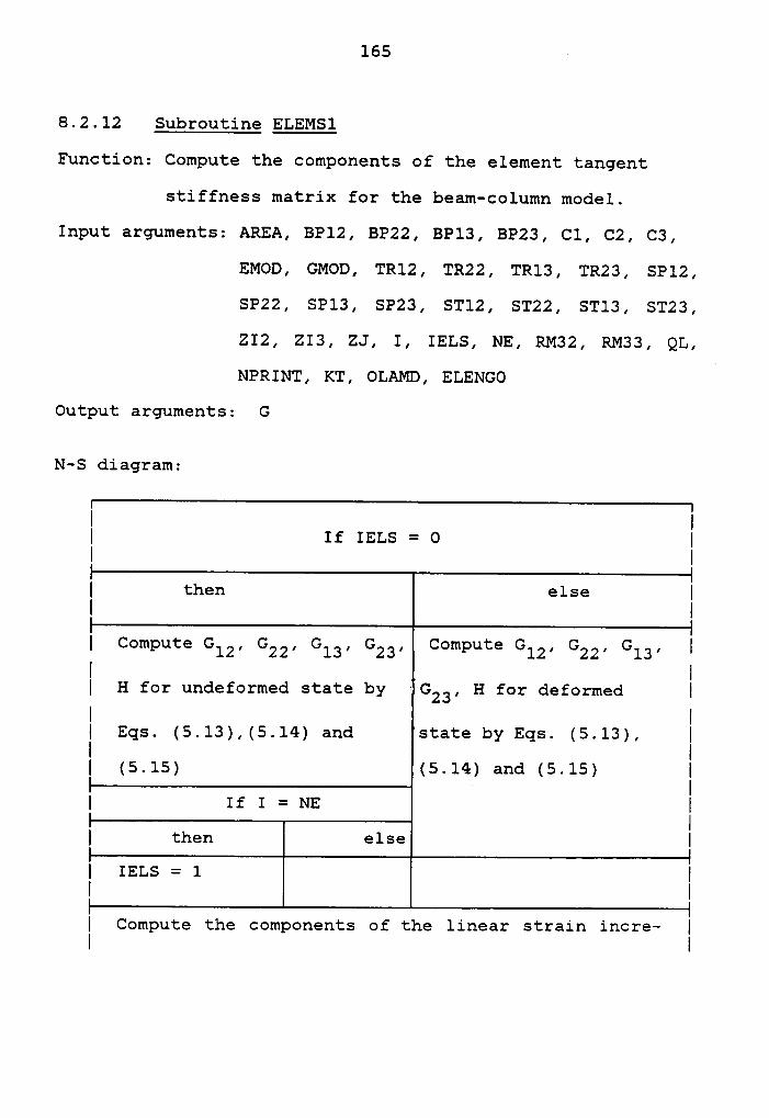
165
8.2.12 Subroutine ELEMS1
Function: Compute the components of the element tangent
stiffness matrix for the beam-column model.
Input arguments: AREA, BP12, BP22, BP13, BP23, Cl, C2, C3,
EMOD, GMOD, TR12, TR22, TR13, TR23, SP12,
SP22, SP13, SP23, ST12, ST22, ST13, ST23,
ZI2, ZI3, ZJ, I, IELS, NE, RM32, RM33, QL,
NPRINT, KT, OLAMD, ELENGO
Output arguments: G
N—S diagram:
I II If IELS = O II II then else II II Compute G12, G22, GI3, G23, Compute G12, G22, GI3, I
I H for undeformed state by ·G23, H for deformed I
I Eqs. (5.13),(5.14) and state by Eqs. (5.13), I
I (5.15) (5.14) and (5.15) I
I If I = NEI
I
I then else I
I IELS = 1
-
II I
{ Compute the components of the linear strain incre- {
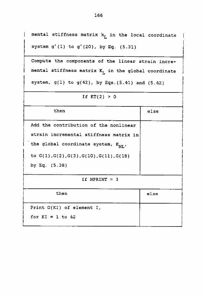
166
I mental stiffness matrix kL in the local coordinate II II system g'(l) to g'(20), by Eq. (5.31) II II Compute the components of the linear strain incre- II II mental stiffness matrix KL in the global coordinate II II system, g(1) to g(42), by Eqs.(5.41) and (5.42) II II If KT(2) > 0 II II then else II II Add the contribution of the nonlinear II II strain incremental stiffness matrix in II _ II the global coordinate system, KNL, II II t¤ @(1).G(2),G(3),G(10).G(11),G(18) II II by Eq. (5.38) II II If NPRINT = 3 II II then else II II Print G(KI) of element I, II II for KI = 1 to 42 II I

167
8.2.13 Subroutine ELEMS2
Function: Compute the components of the element tangent
stiffness matrix for the finite element model.
Input arguments: AREA, Cl, C2, C3, ELENGO, EMOD, GMOD, I,
ZI2, ZI3, ZJ, KT, QL, OLAMD
Output arguments: G
N-S diagram:
I II Initialize the components of the lcoal element tan- I
gant stiffness matrix tozeroI
If KT(l) > O II II then else II II Compute the components of the linear strain I
I incremental stiffness matrix in the local I
I coordinate system, RL II II If KT(2) > O II II then else II II Compute the components of the nonlinear I
I strain incremental stiffness matrix in the I
I local coordinate system, RNL I
I I

168
I Compute the components of the global element tan- II II gent stiffness matrix, Kl
II I
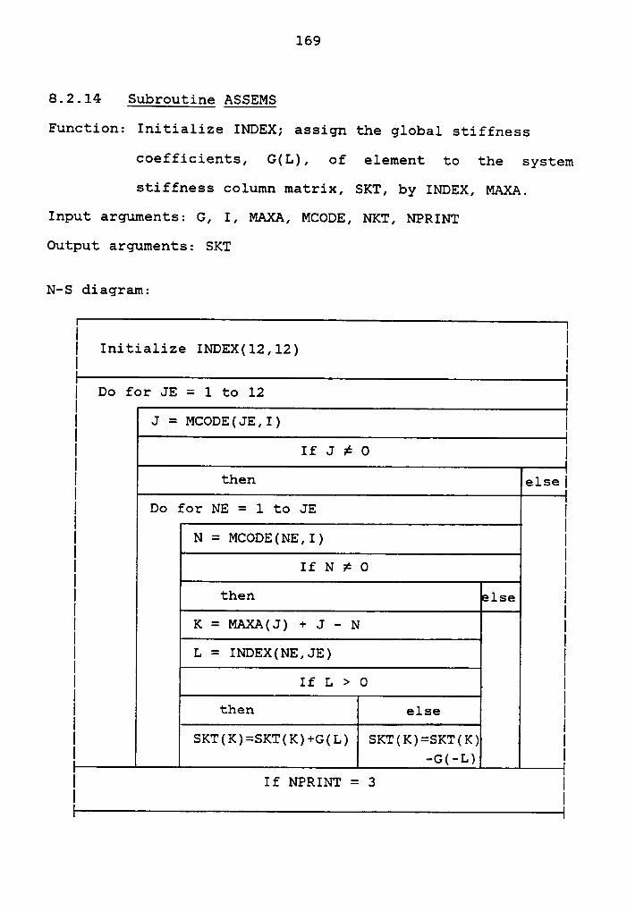
169
8.2.14 Subroutine ASSEMS
Function: Initialize INDEX; assign the global stiffness
coefficients, G(L), of element to the system
stiffness column matrix, SKT, by INDEX, MAXA.
Input arguments: G, I, MAXA, MCODE, NKT, NPRINT
Output arguments: SKT
N-S diagram:
I II
Initialize INDEX(l2,12)I
I Do for JE = 1 to 12 I
I J = MCODE(JE,I) I
I If J # O II then elsel
I Do for NE = 1 to JE I
I N = MCODE(NE,I) II If N ¢ O I
I then -lse I
I K = MAXA(J) + J - N I
I L = INDEX(NE,JE) I
I If L > O I
I then else I
I SKT(K)=SKT(K)+G(L) SKT(K)=SKT(K) II -c(-L) I
I If NPRINT = 3 I
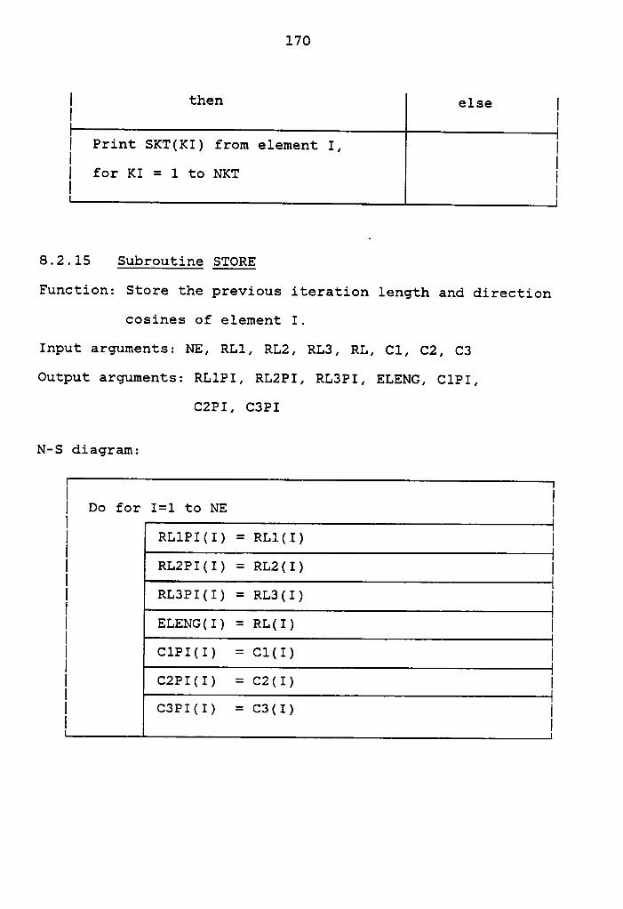
170
I then else II
'
II Print SKT(KI) from element I, I
I for KI = l to NKT II I
8.2.15 Subroutine SQQRE
Function: Store the previous iteration length and direction
cosines of element I.
Input arguments: NE, RLl, RL2, RL3, RL, C1, C2, C3
Output arguments: RL1PI, RLZPI, RL3PI, ELENG, ClPI,
CZPI, C3PI
N-S diagram:
I II Do for I=1 to NE I
I RL1PI(I) = RL1(I) I
I RL2PI(I) = RL2(I) I
I RL3PI(I) = RL3(I) I
I ELENG(I) = RL(I) I
I C1PI(I) = Cl(I) I
I C2PI(I) = C2(I) I
EC3PI(I) = C3(I)
I
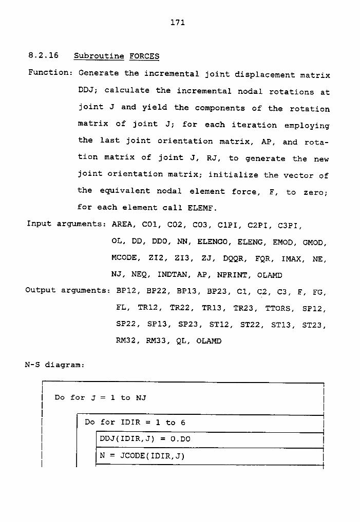
171
8.2.16 Subroutine FORCES
Function: Generate the incremental joint displacement matrix
DDJ; calculate the incremental nodal rotations at
joint J and yield the components of the rotation
matrix of joint J; for each iteration employing
the last joint orientation matrix, AP, and rota-
tion matrix of joint J, RJ, to generate the new
joint orientation matrix; initialize the vector of
the equivalent nodal element force, F, to zero;
for each element call ELEMF.
Input arguments: AREA, COl, CO2, CO3, C1PI, C2PI, C3PI,
OL, DD, DDO, NN, ELENGO, ELENG, EMOD, GMOD,
MCODE, ZI2, ZI3, ZJ, DQQR, FQR, IMAX, NE,
NJ, NEQ, INDTAN, AP, NPRINT, OLAMD
Output arguments: BP12, BP22, BP13, BP23, Cl, C2, C3, F, FG,
FL, TR12, TR22, TR13, TR23, TTORS, SP12,
SP22, SP13, SP23, ST12, ST22, ST13, ST23,
RM32, RM33, QL, OLAMD
N-S diagram:
I I|DoforJ=ltoNJ I
I|Do for IDIR = 1 to 6 I
I DDJ(IDIR,J) = O.DO I
N = JCODE(IDIR,J) I
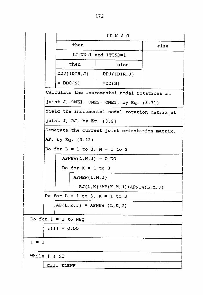
172
I If N ¢ 0 I{ then else |{ If NN=l and ITIND=1 |{ then else {{ DDJ(IDIR,J) DDJ(IDIR,J) {
{ = DDO(N) =DD(N) {
{ Calculate the incremental nodal rotations at |
{ joint J, OME1, OME2, OME3, by Eq. (3.11) {
{ Yield the incremental nodal rotation matrix at {
{ joint J, RJ, by Eq. (3.9) {
{ Generate the current joint orientation matrix, I{ AP, by Eq. (3.12) {
{ Do for L = 1 to 3, M = 1 to 3 {
{ APNEw(L,M,J) = O.DO I{ Do for K = 1 to 3
A{
{ APNEw(L,M,J) |{ = RJ(L,K)*AP(K,M,J)+APNEW(L,M,J) {
{ Do for L = 1 to 3, K = 1 to 3 I
{ AP(L,K,J) = APNEW (L,K,J){
{ Do for I = 1 to NEQ I{ s(1) = 0.00 II { II 1 = 1 II II wmie 1 6 ms: I{ { ca11 ELEME I
173 _
II
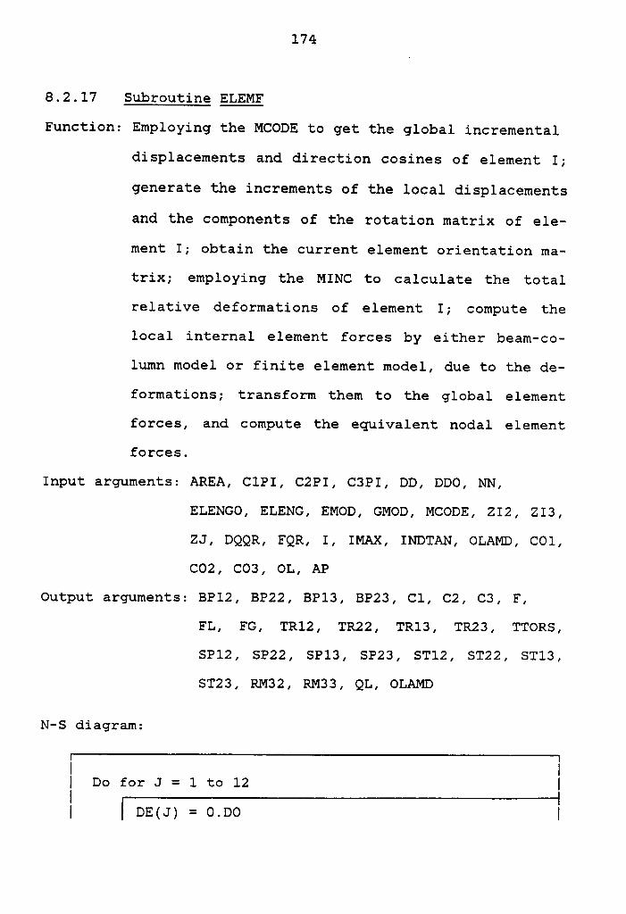
174
8.2.17 Subroutine ELEMF
Function: Employing the MCODE to get the global incremental
displacements and direction cosines of element I;
generate the increments of the local displacements
and the components of the rotation matrix of ele-
ment I; obtain the current element orientation ma-
trix; employing the MINC to calculate the total
relative deformations of element I; compute the
local internal element forces by either beam—co-
lumn model or finite element model, due to the de-
formations; transform them to the global element
forces, and compute the equivalent nodal element
forces.
Input arguments: AREA, ClPI, C2PI, C3PI, DD, DDO, NN,
ELENGO, ELENG, EMOD, GMOD, MCODE, ZI2, ZI3,
ZJ, DQQR, FQR, I, IMAX, INDTAN, OLAMD, COl,
CO2, CO3, OL, AP
Output arguments: BPl2, BP22, BP13, BP23, C1, C2, C3, F,
FL, FG, TR12, TR22, TR13, TR23, TTORS,
SP12, SP22, SP13, SP23, STl2, ST22, ST13,
ST23, RM32, RM33, QL, OLAMD
N-S diagram:
I Il Do for J = 1 to 12 II I DE(J) = 0.00 I
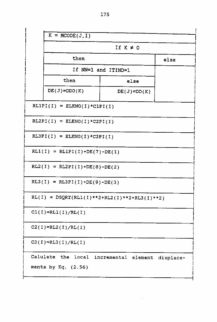
175
I I{
K = MCODE(J,I)I
{ If 1< ¢ 0 I
I I{ If NN=1 and ITIND=1 I
I{ then else II
{DE(J)=DDO(K) DE(J)=DD(K) I
I
{RL1PI(1) = ELENG(I)*ClPI(I) I
II—————————·——————————————————————————————————————————————4I RL2P1(1) = ELENc(1)*c2P1(1) II IP-·——————·————————————·—————————·—————·—————————————————4I RL3P1(1) = ELENG(I)*C3PI(I) II IF--———————————————————————————————————————————————%I RLl(I) = RL1P1(1)+DE(7)-DE(1) II IF———————————————————————————————————————————————————————4I RL2(I) = RL2P1(1)+DE(8)-DE(2) II IF-—————————————·—·—————————·———————————·——————————·——————4I RL3(I) = RL3PI(I)+DE(9)—DE(3) II IP————————··————————————·———————————————————————————————————II RL(1) = DsQRT(RL1(I)**2+RL2(1)**2+RL3(1)**2) II IP-————————————————————————————————————————————————————————%I Cl(I)=RL1(I)/RL(I) II II-——————————————————————————————·———————————————————————%I c2(1)=RL2(1)/RL(1) II IP-———————————————————————————————————————————————————————%I C3(I)=RL3(I)/RL(I)
{IF——————————————————————————————————————————————————————%I Calulate the local incremental element displace— II II ments by Eq. (2.56)
{IF————————————————————————————————————————————————————%
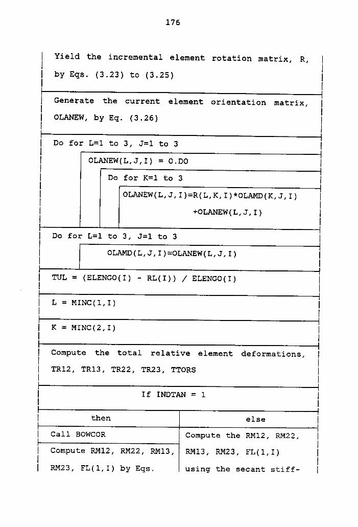
176
I Yield the incremental element rotation matrix, R, I
I by Eqs. (3.23) to (3.25) II II Generate the current element. orientation matrix, I
I OLANEW, by Eq. (3.26) II II Do for L=l to 3, J=l to 3 I
I OLANEW(L,J,I) = O.DO I
I Do for K=l to 3 I
I OLANEW(L,J,I)=R(L,K,I)*OLAMD(K,J,I) I
I +0LANEw(L,J,I) II II Do for L=1 to 3, J=l to 3 I
II
OLAMD(L,J,I)=OLANEw(L,J,I)I
ITUL = (ELENGO(I) — RL(I)) / ELENGO(I)
I
I L = MINC(1,I) II II K = MINC(2,I) II II Compute the total relative element deformations, I
I TR12, TR13, TR22, TR23, TTORSI
I If INDTAN = 1I
I then else I
I Call BOWCOR Compute the RMl2, RM22, I
I Compute RMl2, RM22, RMl3, RMl3, RM23, FL(l,I) I
I RM23, FL(l,I) by Eqs. using the secant stiff- I
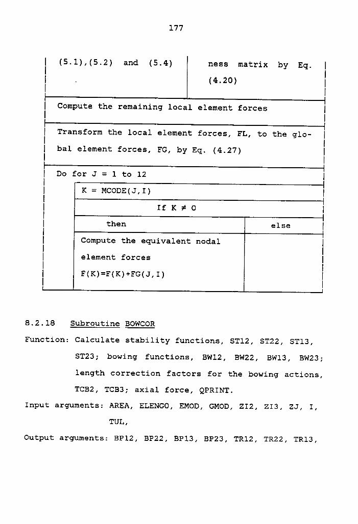
177
I (5.l),(5.2) and (5.4) ness matrix by Eq. II _ (4.20) II II Compute the remaining local element forces II II Transform the local element forces, FL, to the glo- I
Ibal element forces, FG, by Eq. (4.27)
I
I Do for J = 1 to 12 II K = MCODE(J,I) II If K ¢ O II then else II Compute the equivalent nodal II element forces I
I F(K)=F(K)+FG(J,I) II I
8.2.18 Subroutine BOWCOR
Function: Calculate stability functions, STl2, ST22, ST13,
ST23; bowing functions, BWl2, BW22, BW13, BW23;
length correction factors for the bowing actions,
TCB2, TCB3; axial force, QPRINT.
Input arguments: AREA, ELENGO, EMOD, GMOD, ZI2, ZI3, ZJ, I,
TUL,
Output arguments: BP12, BP22, BP13, BP23, TRl2, TR22, TRl3,
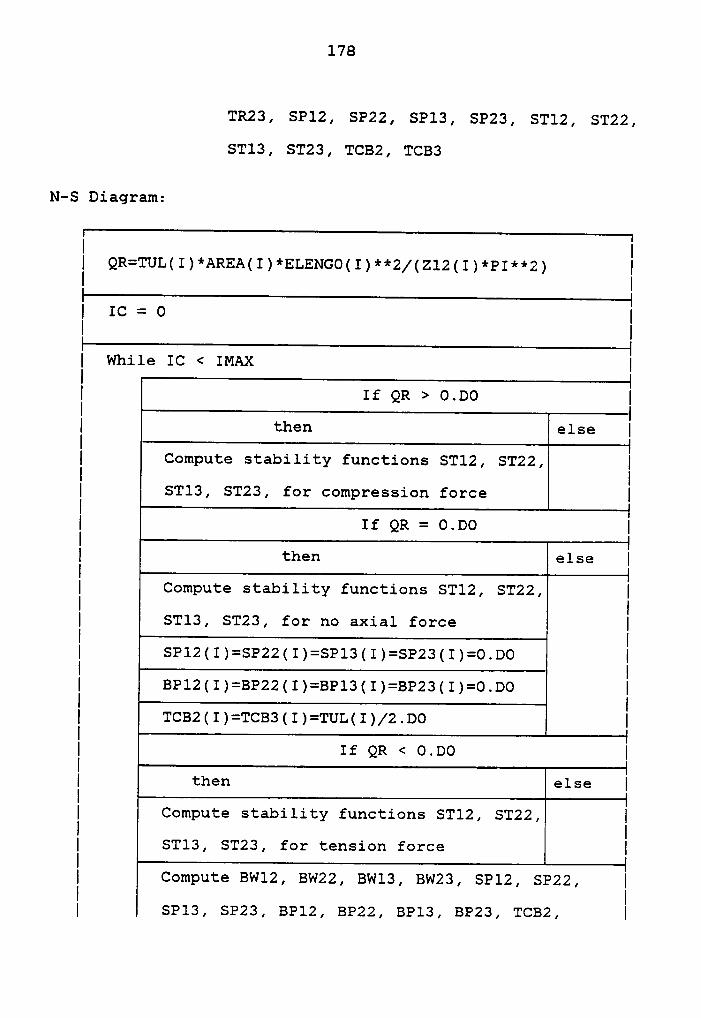
178
TR23, SP12, SP22, SPl3, SP23, STl2, ST22,
ST13, ST23, TCB2, TCB3
N-S Diagram:
I II
QR=TUL(I)*AREA(I)*ELENGO(I)**2/(Z12(I)*PI**2)I
I IC = O II II While IC < IMAX I
I If QR > O.DO I
I then else I
I Compute stability functions ST12, ST22, I
I STl3, ST23, for compression force I
I If QR = O.D0 I
I then else I
I Compute stability functions STl2, ST22, I
I STl3, ST23, for no axial force I
I SPl2(I)=SP22(I)=SPl3(I)=SP23(I)=O.DO I
I BPl2(I)=BP22(I)=BP13(I)=BP23(I)=O.DO I
I TCB2(I)=TCB3(I)=TUL(I)/2.DO I
I If QR < O.DO I
I then else I
I Compute stability functions ST12, ST22, I
I ST13, ST23, for tension force I
I Compute BW12, BW22, BWl3, BW23, SP12, SP22, I
I SP13, SP23, BP12, BP22, BP13, BP23, TCB2, I

179
| TCB3, TCBZP, TCB3P |] Compute FQRC and DQ (ref. [29]) |
E QR = QR + DQ I| DQQRC = DABS(DQ/QR) |
] IC = IC + 1 |] If DQ/QR s DQQR and |] FQRC s FQR ]
] then else |] IC = IMAX + 1 |] If DQ/QR > DQQR or |
] FQRC > FQR ]] then else |
Stop {
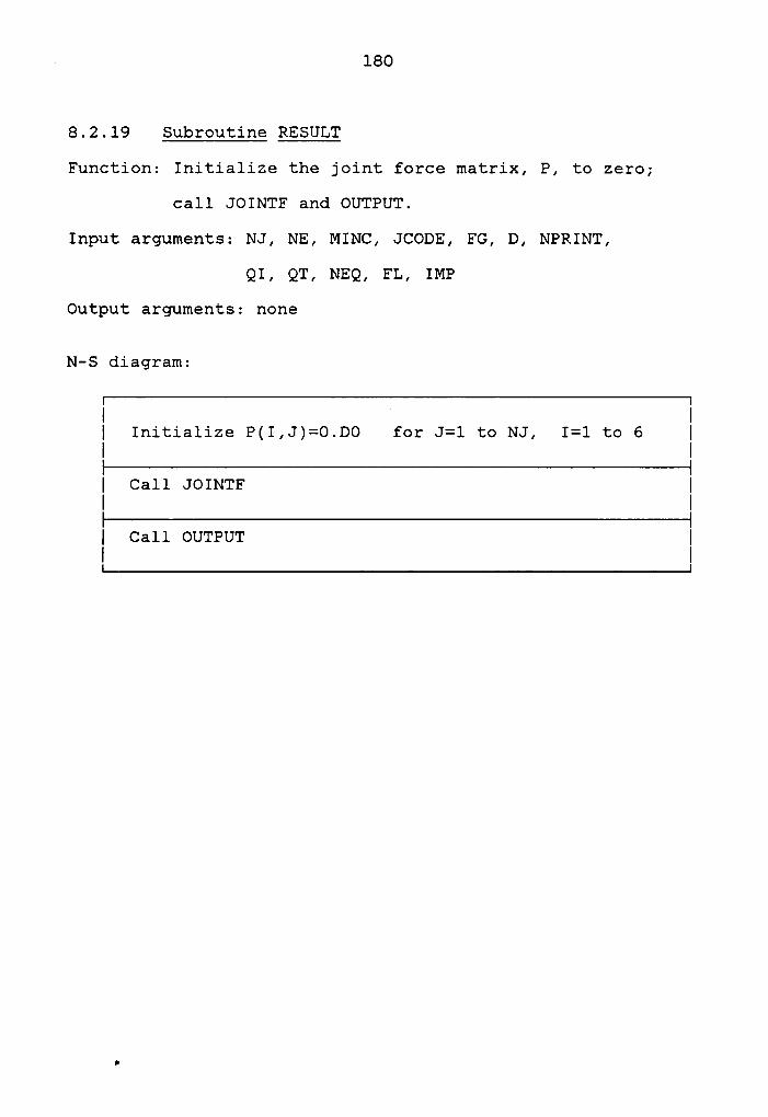
- 18O
8.2.19 Subroutine RESULT
Function: Initialize the joint force matrix, P, to zero;
call JOINTF and OUTPUT.
Input arguments: NJ, NE, MINC, JCODE, FG, D, NPRINT,
QI, QT, NEQ, FL, IMP
Output arguments: none
N—S diagram:
I II Initialize P(I,J)=O.DO for J=l to NJ, I=l to 6 II I| ca11 Jomnrr |I I
I ca11 oUT1¤UT IL..................................................._..J

181
8.2.20 Subroutine JOINTF
Function: Assign the global element forces, FG, to the
joint force matrix, P, via MINC.
Input arguments: NE, MINC, FG
Output arguments: P
N-S diagram:
V"'——”“—-——_—'_"—_°"_—___——”—_—_—_'—-—"‘-“'-—_—“—_‘-7
{ Do for I = 1 to NE {{ J = MINC(1,I) |{ K = MINC(2,I) . |{ Do for L = 1 to 6 {{ P(L,J) = P(L,J)+FG(L,I) . |
EP(L,K) = P(L,K)+FG(L+6,I)
{
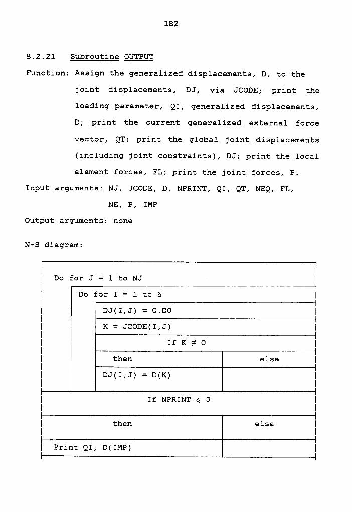
182
8.2.21 Subroutine OUTPUT
Function: Assign the generalized displacements, D, to the
joint displacements, DJ, via JCODE; print the
loading parameter, QI, generalized displacements,
D; print the current generalized external force
vector, QT; print the global joint displacements
(including joint constraints), DJ; print the local
element forces, FL; print the joint forces, P.
Input arguments: NJ, JCODE, D, NPRINT, QI, QT, NEQ, FL,
NE, P, IMP
Output arguments: none
N—S diagram:
I II Do for J = 1 to NJ · I
I D8 £8: 1 = 1 c8 6 |
I DJ(1,J) = o.D0 |
I K = JcoDE(1,J) |
I If K ¢ 0 II then else I
I DJ(I„J) = D(K) II I
I If NPRINT 6 3 II II then else II
'
II Print QI, D(IMP) I

183
I If NPRINT = 4 II then else II II Print QI I
I Print QT(I) for I = l to NEQ I
I Print DJ(I,J) for I=l to 6, J=l to NJ I
I Print FL(I,J) for I=1 to 12, J=l to NE I
I Print P(I,J) for I=l to 6, J=l to NJE
Chapter IX
CONCLUSION
9.1 CONCLUSION
Updated Lagrangian and a total Lagrangian formulations of
a geometrically‘ nonlinear three—dimensional beam element,
undergoing large displacements with small strain, have been
developed. In the T.L. formulation the incremental linear
strains Oeij (Eqs. (2.63) and (2.76)) contain an initial
displacement effect that leads to a more complex strain—dis—
placement matrix than in the U.L. formulation. The main
difference between the U.L. and the T.L. formulations is
that in the T.L. formulation the interpolation functions in
Eq. (2.74) are obtained by referring the displacements to
the initial configuration and the äBLl matrix (Eq. 2.9lc)
is included in the calculations.
It was been shown in Chapter' 2 that two formulations
yield identical element stiffness matrices and vectors of
nodal element forces. In fact, if the appropriate constitu-
tive relations are employed, same results are obtained. In
this study for three dimensional beam element with small de-
formations and uniaxial strain, the same Young's modulus
184
185l
used in the T.L. and U.L. formulations yields practically
the same results.
The choice of using either the U.L. or the T.L. formula-
tion depends on their numerical efficiency, i.e., economy.
Which formulation is most effective depends on the program
design and the actual structures.
The finite element model and the beam-column model have
been compared for space frame problems. Both the linear and
nonlinear strain incremental stiffness matrices must be con-
sidered in both models in order to predict the response ac-
curately and to detect instability of large displacement
problems. The finite element model is simple in theory, but
quite a number of elements are often needed for satisfactory
accuracy. The beam-column model uses the conventional beam-
column theory to determine the member force-deformation re-
lations so that fewer elements are often needed than in the
case of a finite element model to give the same accuracy.
Because the stability functions cmn in the beam-column
model depend on whether the axial force is compressive,
zero, or tensile, the axial force must be determined by an
iterative procedure (i.e. Newton method). Consequently, more
186computationaleffort is required in the beam-column model
than in the finite element model for the same mesh.
From the sample analyses (chapter 7) it is seen that both
element models are reliable for studying the behavior of
space frames. In conclusion the following observations are
presented:
The only disadvantage of the finite element model is that a
fine mesh is often needed for satisfactory accuracy. The
main advantages of the finite element model are:
1. The formulations are simple without recourse to com-
plex differential equations.
2. It can be extended to the elements undergoing large
deformations in which the cross-sectional area would
be updated.
3. The material properties can be adjusted at each ele-
ment integration point. Combinations of material non-
linearity and geometric nonlinearity is particularly
simple if the increment of the material properties
may be obtained. The operations required in the solu-
tion of problems of material and geometric nonlinear-
ity are similar.
4. The external loads can. be configuration-dependent,
i.e., nonconservative forces, like follower forces
can be involved [48].
187
On the other hand, the main advantage of the beam-column mo-
del is that it yields higher accuracy than the finite ele-
ment model for the same mesh. However, the disadvantages of
the beam-column model are:
l. The formulations are complicated by the fact that the
stability coefficients (appendix B) are functions of
the axial force which must be obtained by an itera-
tive procedure.
2. The basic element force-deformation relations (sec.
5.2) are derived from the conventional beam-column
theory [23]; thus the relative deformations of the
element are limited to be small.
3. Since the formulations are based on elastic behavior
(sec. 5.2), extensions to material nonlinearity is
impratical.
4. The external loads are assumed to be configuration-
independent, i.e., conservative forces, and applied
at the nodes only.
188
9.2 SUGGESTIONS Egg FUTURE DEVELOPMENT
Some interesting extensions of the present study are sug-
gested:
1. Implement the T.L. formulation in the computer pro-
gram using both models by transformation of the in-
terpolation functions [9].
2. Use numerical integration, that is, Newton-Cotes or
Gauss integration [38], to evaluate the vectors of
nodal element forces.
3. Include the material nonlinearity in the finite ele-
ment model.
4. The displacements in the U.L. formulation referred to
the current coordinates at time t are usually small
enough thatKNL
can be omitted [33]. The effects of
neglecting the nonlinear strain incremental stiffness
matrix in the U.L. formulation can be studied.
5. Different convergence criteria will effect the accu-
racy and computer cost. The effects of using diffe-
rent convergence criteria in nonlinear analysis are
of interest.
6. A comparative study of different numerical solution
techniques in nonlinear analysis.
189
7. The final goal is to develop a nonlinear dynamic ana-
lysis program to analyze space frames under earthq—
uake loads.
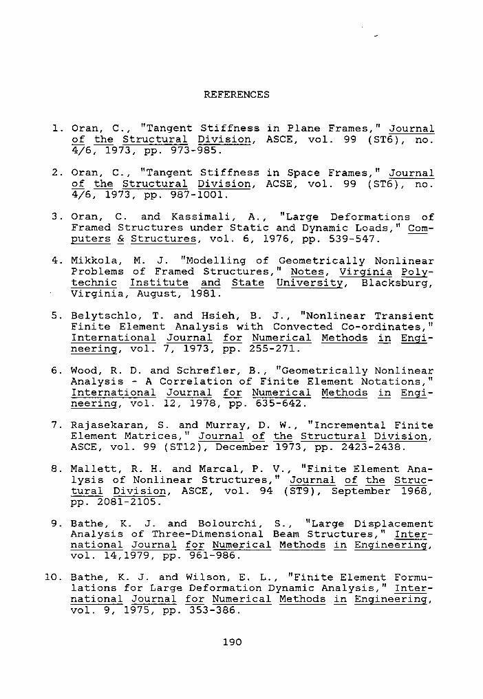
REFERENCES
1. Oran, C., "Tangent Stiffness in Plane Frames," Journalgg the Structural Division, ASCE, vol. 99 (ST6), no.4/6, 1973, pp. 973-985.
2. Oran, C., "Tangent Stiffness in Space Frames," Journalgg the Structural Division, ACSE, vol. 99 (ST6), no.4/6, 1973, pp. 987-1001.
3. Oran, C. and Kassimali, A., "Large Deformations ofFramed Structures under Static and Dynamic Loads," Com-puters Q Structures, vol. 6, 1976, pp. 539-547.
4. Mikkola, M. J. "Modelling of Geometrically NonlinearProblems of Framed Structures," Notes, Virginia Poly-technic Institute and State University, Blacksburg,
· Virginia, August, 1981.
5. Belytschlo, T. and Hsieh, B. J., "Nonlinear TransientFinite Element Analysis with Convected Co—ordinates,"International Journal for Numerical Methods gp Engi-neering, vol. 7, 1973, pp. 255-271.
6. Wood, R. D. and Schrefler, B., "Geometrically NonlinearAnalysis - A Correlation of Finite Element Notations,"International Journal for Numerical Methods ig; Engi-neering, vol. 12, 1978, pp. 635-642.
7. Rajasekaran, S. and Murray, D. W., "Incremental FiniteElement Matrices," Journal gg the Structural Division,ASCE, vol. 99 (ST12), December 1973, pp. 2423-2438.
8. Mallett, R. H. and Marcal, P. V., "Finite Element Ana-lysis of Nonlinear Structures," Journal gg the Struc-tural Division, ASCE, vol. 94 (ST9), September 1968,pp. 2081-2105.
9. Bathe, K. J. and Bolourchi, S., "Large DisplacementAnalysis of Three—Dimensional Beam Structures," Inter-national Journal for Numerical Methods gg Engineering,vol. 14,1979, pp. 961-986.
10. Bathe, K. J. and Wilson, E. L., "Finite Element Formu-lations for Large Deformation Dynamic Analysis," Inter-national Journal for Numerical Methods gg Engineering,vol. 9, 1975, pp. 353-386.
190

191
11. Carey, G. F., "A Unified Approach to Three Finite Ele-ment Theories for Geometric Nonlinearity," ComputerMethods ip Applied Mechanics and Engineering, vol. 4,1974, pp. 69-79.
12. Hibbitt, H. D., Marcal, P. V. and Rice, J. R., "A Fi-nite Element Formulation for Problems of Large Strainand Large Displacement," Int. Q. pg Solids And Struc-tures, vol. 6, 1970, pp. 1069-1086.
13. Holden, J. T., "On the Finite Deflections of ThinBeams," Int. Q. pg Solids and Structures, vol. 8, 1972,pp. 1051-1055.
14. Felippa, C. A., "Procedures for Computer Analysis ofLarge Nonlinear Structural Systems," Large EngineeringSystems, Proceedings of the International SymposiumHeld at the University of Manitoba, Winnipeg, Manitoba,Canada, August 1976, pp. 60-100.
15. Becker, Eric B., Carey, Graham F. and Oden, Tinsley J.,"Finite Elements, An Introduction," vol. 1, pp. 87-131.
16. Connor, J. J., Logcher, R. D. and Chan, S. C., "Nonli-near Analysis of Elastic Framed Structures," Journal pgthe Structural Division, ASCE, vol. 94 (ST6), June1968, pp. 1525-1545.
17. Belytschko, T. and Schwer, L., "Large Displacement,Transient Analysis of Space Frames," InternationalJournal for Numerical Methods gp Engineering, vol. 11,1977, pp. 65-84.
18. Tang, S. C., Yeung, K. S. and Chon, C. T., "On the Tan-gent Stiffness Matrix in a Convected Coordinates Sys-tem," Computers Q Structures, vol. 12, 1980, pp.849-856.
19. Remseth, S. N., "Nonlinear Static and Dynamic Analysisof Framed Structures," Computers Q Structures, vol. 10,pp. 879-897.
20. Wood, R. D. and Zienkiewicz, 0. C., "Geometrically Non-linear Finite Element Analysis of Beams, Frames, Archesand Axisymmetric Shells," Computers Q Structures, vol.7, 1977, pp. 725-735.
21. Papadrakakis, M., "Post-Buckling Analysis of SpatialStructures by Vector Iteration Methods," Computers QStructures, vol. 14, 1981, pp. 393-402.
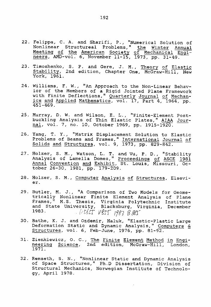
192
22. Felippa, C. A. and Sharifi, P., "Numerical Solution ofNonlinear Structureal Problems," the Winter AnnualMeeting pi the American Society pg: Mechanical Engi-neers, AMD-vol. 6, November 11-15, 1973, pp. 31-49.
23. Timoshenko, S. P. and Gere, J. M., Theory pg ElasticStability, 2nd edition, Chapter One, McGraw-Hill, NewYork, 1961.
24. Williams, F. W., "An Approach to the Non—Linear Behav-ior of the Members of a Rigid Jointed Plane Frameworkwith Finite Deflections," Quarterly Journal pg Mechan-ics and Applied Mathematics, vol. 17, Part 4, 1964, pp.451-469.
25. Murray, D. W. and Wilson, E. L., "Finite-Element Post-buckling Analysis of Thin Elastic Plates," AIAA Jour-nal, vol. 7, no. 10, October 1969, pp. 1915-1920.
26. Yang, T. Y., "Matrix Displacement Solution to ElasticProblems of Beams and Frames," International Journal pgSolids and Structures, vol. 9, 1973, pp. 829-842.
27. Holzer, S. M., Watson, L. T. and Vu, P. D., "StabilityAnalysis of Lamella Domes," Proceedings pg ASCE 1981Annal Convention and Exhibit, St. Louis, Missouri, Oc-tober 26-30, 1981, pp. 179-209.
28. Holzer, S. M., Computer Analysis pj Structures, Elsevi-er.
29. Butler, M. J., "A Comparison of Two Models for Geome-trically Nonlinear Finite Element Analysis of PlaneFrames," M.S. Thesis, Virginia Polytechnic Instituteand State University, Blacksburg, Virginia, December
1983-30.Bathe, K. J. and Ozdemir, Haluk, "Elastic—Plastic LargeDeformation Static and Dynamic Analysis," Computers QStructures, vol. 6, Feb—June, 1976, pp. 81-92.
31. Zienkiewicz, O. C., The Finite Element Method lp Engi-neering Science, 2nd edition, McGraw-Hill, London,1971.
32. Remseth, S. N., "Nonlinear Static and Dynamic Analysisof Space Structures," Ph.D Dissertation, Division ofStructural Mechanics, Norwegian Institute of Technolo-gy, April 1978.
193
33. Cook, R. D., Concepts and Applications pg Finite Ele-ment Analysis, 2nd edition, John-Wiley ] Sons, London,1981.
34. Desai, C. S., Elementary Finite Element Method, Pren-tice-Hall Inc., N.J., 1979.
35. Young, J. W., "A Computer Simulation of Nonlinear Tran-sient Response of Structures," Automobile Manufactur-ers' Association and the National Highway Traffic Safe-py Administration, DOT-HS-091-1-125-B, March 1972.
36. Glowinski, R., Rodin, E. Y. and Zienkiewicz, 0. C., Ep-ergy Methods ip Finite Element Analysis, 1979.
37. Fung, Y. C., Foundations pf Solid Mechanics, Prentice-Hall Inc., N.J., 1965.
38. Bathe, K. J., Finite Element Procedures lp EngineeringAnalysis, Prentice-Hall Inc., N.J., 1982.
39. Chu, Kuang-Han and Rampetsreiter, R. H., "Large Deflec-tion Buckling of Space Frames," Journal pf the Struc-tural Division, ASCE, vol. 98 (ST12), December 1972,pp. 2701-2722.
40. Dickie, J. F. and Broughton, "Geometric Nonlinearity,"Journal pf Structural Mechanics, 1(2), 1972, pp.249-266.
41. Murray, D. W. and Wilson, E. L., "Finite-Element LargeDeflection Analysis of Plates," Engineering MechanicsDivision, ASCE, vol. 95, (EM1), 1969, pp. 143-165.
42. Yaghmai, S. and Popov, E. P., "Incremental Analysis ofLarge Deflections of Shells of Revolution, " Interna-tional Journal pf Solids and Structures, vol. 7, no.10, 1971, pp. 1375-1393.
43. Ramm, E., "Strategies for Tracing Nonlinear ResponseNear Limit Points," Europe-U.§.-Workshop: Nonlinear Fg-nite Element Analysis lp Structural Mechanics, July28-31, 1980, Bochum, G. F. R,.
44. Gallagher, R. H., Yamada, Y. and Oden, T., Recent Ag-vances ip Matrix Methods pf Structural Analysis and Dp-sign, The University of Alabama in Huntsville, Alabama,August 1969.
194
45. Riks, E., "The Application of Newton's Method to theProblem of Elastic Stability, " Journal pf Applied Mp-chanics, vol. 39, 1972, pp. 1060-1066.
46. Wempner, G. A., "Discrete Approximatons Related to Non-linear Theories of' So1ids," International Journal pgSolids And Structures, vol. 7, 1971, pp. 1581-1599.
47. Crisfield, M. A., "A Fast Incremental/Iterative Solu-tion Procedure That Handles Snap-Through," Computers QStructures, vol. 13, 1981, pp. 55-62.
48. Katzenberger, G. S.,"Geometrically Nonlinear Analysisof Pressure-Loaded Arches, Rings, and Frames Using aFollower Force Algorithm", M. S. Thesis, Virginia Po-lytechnic Institute and State University, Blacksburg,Virginia, August, 1983.
49. Bathe, K. J. and Cimento, A. P., "Some Practical Proce-dures for the Solution of Nonlinear Finite ElementEquations," Journal pf Computer Methods gp Applied Mg-chanics and Engineering, vol. 22, 1980, pp. 59-85.
50. Bergan, P. G. and Soreide, T. H., "Solution of LargeDisplacement and Instability Problems Using the CurrentStiffness Parameter," Finite Elements ip Nonlinear Mg-chanics, vol. 2, 1977, pp. 647-669.
51. Holzer, S. M., Plaut, R. H., Somers, A. E. and White,W. S., "Stability of Lattice Structures under CombinedLoads," Journal pf the Engineering Mechanics Division,ASCE, vol. 106, No. EM2, April, 1980, pp. 289-305.
52. Hangai, Y. and. Kawamata, S., "Nonlinear Analysis ofSpace Frames and Snap-Through Buckling of ReticulatedShell Structures," IASS Pacific Sypposiunx Part Il_ ppTension Structures and Space Frames, Tokyo and Kyoto,Paper No. 9-4, 1972, pp. 803-816.
53. Paradiso, M. and Tempesta, G., "Member Buckling Effectsin Non-linear Analysis of Space Trusses," NumericalMethods for Non-linear Problems, vol. 1, September,1980, pp. 395-405.
54. The Aluminum Association, "Specifications for AluminumStructures," Construction Manual Series, Section 1, NewYork, N.Y., April,1982.
195
55. Uliana, D., "The Effects of Earthquake Excitations onReticulated Domes," M. S. Thesis, Virginia PolytechnicInstitute and State University, Blacksburg, Virginia,March,l985.

Appendix A
JOINT ORIENTATION MATRIX aj FOR SMALL JOINTROTATIONS
In this appendix Eq. (3.9) will be derived for small
joint rotation. A small change in the orientation of the
joint can be represented by rotation components pl, p2, p3,
in the global coordinates X1, X2, X3 (Fig. A.l). Let
P1P = P2P3
To derive Eq. (3.9) we can formulate the joint orienta-
tion matrix in three steps:
First, consider Fig. A.2 which shows a small joint rota-
tion p2 about X2-axis, similar to Eq. (3.1)
b = ajz XI
(A.2)
where
cos p2 cos 90° cos(9OO+p2)
ajz = cos 9o° cpp 0° pps 9o° (A.2)cos(9O°-p2) cos 90° cos p2
196

197
For infinitesimal p2:
p2 = O , cos p2 = 1 , sin P2 = P2 (A.4)
Substituting Eq. (A.4) into (A.3), we have
1 O -.p2
ajz = O 1 O (A.5)
p2 O l
Second, we rotate a small joint rotation p3 about b3-axis
(Fig. A.3). In a similar manner we have
a = ¤j3 b (A.6)
where
1 p3 O
°j3 = -p3 1 O (A.7)
O O 1
Third, we rotate a small joint rotation pl about al—axis
(Fig. A.4). Similarly
y = ajl a (A.8)
where
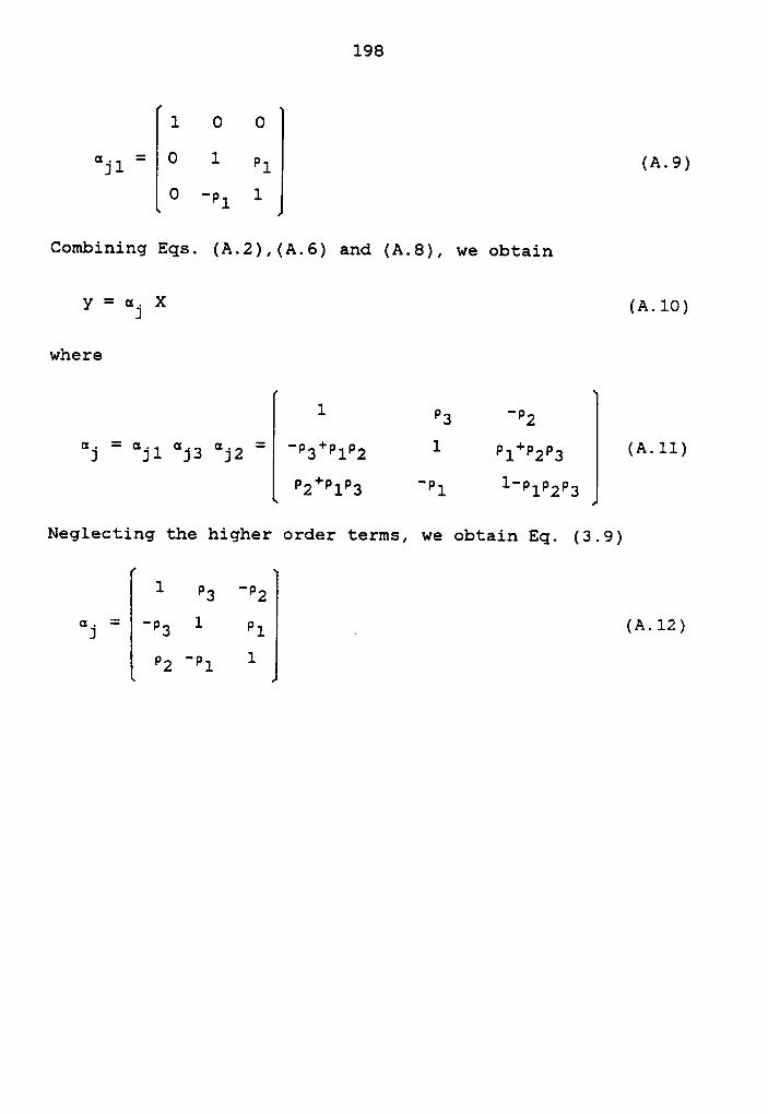
198
1 O O
ajl = O l pl (A.9)
O -pl l
Combining Eqs. (A.2),(A.6) and (A.8), we obtain
y = aj X (A.lO)
where
1 P3 ·P3°‘3 = ajl °‘js °‘j2 = '°3‘”"1°2 1 "1+"2"2 (All)
P2+P1P3 —pll"PlP2P3
Neglecting the higher order terms, we obtain Eq. (3.9)
1 P3 ·P3aj = -p3 1plP2
·p1 1

199
X2yly2P2
p I1 XI pl
1\\\| //
/ arX5A . 3
Fig• A.l Small Joint Rotation
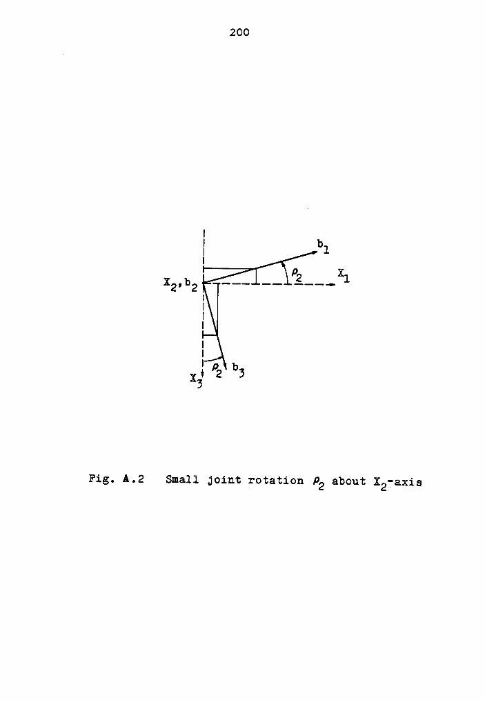
200
I b} 1
P X2 1"'i" ** iii?IIII
I
IXI‘°2 bz
3
Fig. A.2 Small joint rotation P2 about X2iaxis
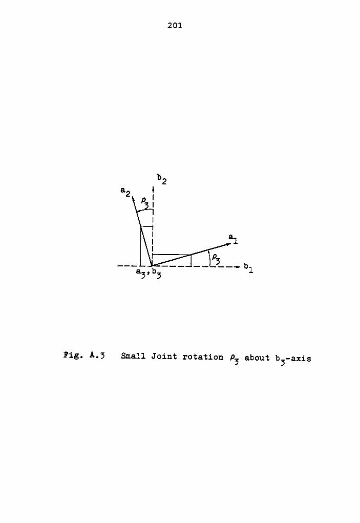
201
bza2
IP I
I
I alI ps
a3,b3
Fig. A.3 Small Joint rotation P3 about b5—axis
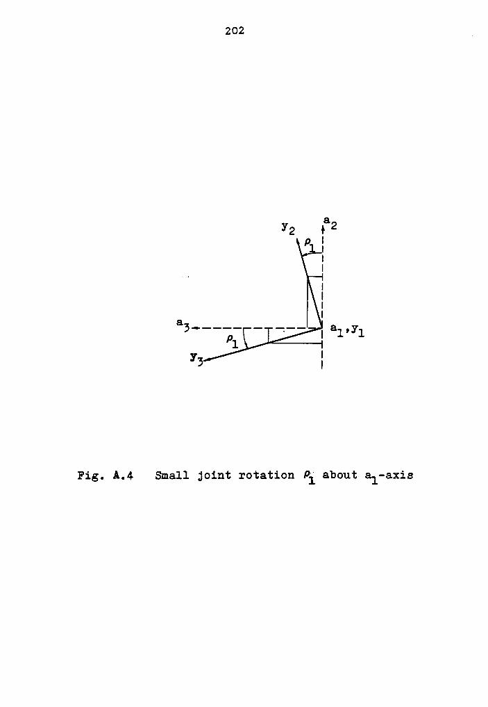
202
8Y22 I 2
p III
222 'III
a I3·———— — «——
I almlpl
I
Fig. A.4 Small joint rotation Pi about al-axis
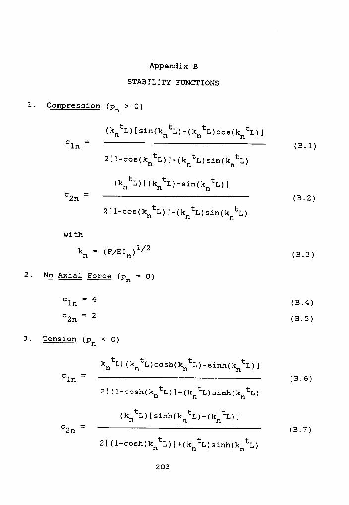
Appendix B
STABILITY FUNCTIONS
1. Compression (pn > O)
Clnwith
kn = (P/EIn)1/2(6.3)
2. gg Axial Force (pn = O)
cln = 4 (B.4)
czn = 2 (B.5)
3. Tension (pn < O)
clnczn203
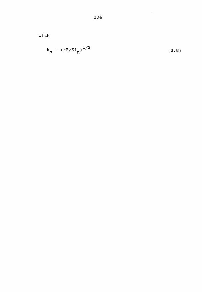
204l
with
kn = (-P/E1n)l/2 (B.8)
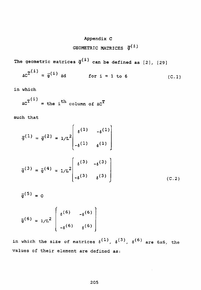
Appendix C
GEOMETRIC MATRICES §4i)
The geometric matrices §(i) can be defined as [2], [29]
(i) _·AcT = gn) Ad :61 1 = 1 cg 6 (c.1)
in which
(i)ACT= the ith column of ACT
such that
ö(l) _ö(l)- - 2g(l) = g(2) = 1/L
_ö(l) 6(l)
ö(3) _6(3)- - 4 2g(3) = g( ) = 1/L
-6n) an)
= O
6(6) _6(6)ä‘6) = 1/L2
_6(6) ö(6)
in which the size of matrices 6(l), 6(3), ö(6) are 6x6, the
values of their element are defined as:
205

206A
ag) = (sg) = 1 0 (C.3)(sg) = (sg) = -1, other (sg) = 0 (0.4)ag) = (sg) = -1, 61:1161: (sir?) = 0 (0.5)
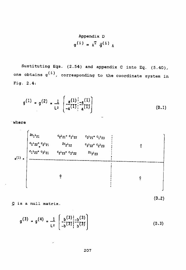
Appendix D
g(i) = AT §(i) A
Sustituting Eqs. (2.54) and appendix C into Eq. (5.40),
one obtains g(i),corresponding to the coordinate system in
Fig. 2.4:
gw . gw . i_g<1>:gg“>
I L2 _,gU7) am (D-1)
‘where
2°1^21 c2x21+ c1Ä22 c3A21+ c1Ä23 EI°1^22”’_°2^21 2c2Ä22 c3X22+ °z^za 9I
• .......-.,.,_,_,__________________________________i________________________“-_-·-
IJI
9 I o
(D.2)Q is a null matrix.
1gw 2 gw 2 i_g‘3’;;p"’
gg 3)L2•
207
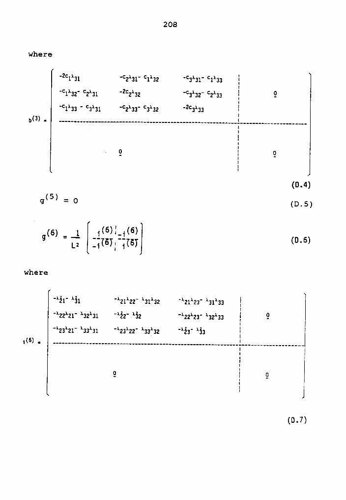
208
where
***1*21 **2*21* *1*22 **2*21* *1*22I**1*22* *2*21 ***2*22 **2*22* *2*22 I 9
I
**1*22 * *2*21 **2*22* *2*22 ***2*22x ••-•-,--.....----.......•.•••••--••-••..••••••••••-•..-....i----..............2..,-2 I1
II
· 9 I 9I
(D.4)5<2I I = O (12. 5)
I1
g(6)= Ä
-i(6)|Zi(6)(Q 5)L2 _iI67; (I6?
where
**51* *51 **21*22* *21*22 **21*22* *21*22 I1**22*21* *22*21 **52* .*52 **22*22* *22*22 I 91
**22*21*. *22*21 **22*22* *22*22 **52* *52 EM6). .............................................................1..,__..,___,_,__,__I1 1E I
0 I 0- 1 -II
(D.7)
Appendix E
NOTATION
A = area of cross section
t t _oBL· tBL ‘linear strain-displacement matrix at time t referred to
configuration at time O, t
t t _0BNL' tBNL ‘
nonlinear strain—displacement matrix at time t referred
to configuration at time O, t
b = bowing functionsmn
= (cln+c2H)(c2¤—2) / Snzqn for m = 1
= czn / 8(cl¤+c2¤) for m = 2
C = local transformation matrix defined in Eq. (5.22)
OCijrs’ tcijrs =
component of incremental material property tensor at
time t referred to configuration at time O, t
OC, tC, t+AtC= element configuration at time O, t, t+At
CPDB = displacement convergence parameter adopted by Bathe
CPDC = displacement convergence parameter adopoted by Cook
CPE = convergence parameter for the unbalanced force
criterion
cbm = length correction factors for bending action_ 2 2—
bln (e1n+€2n) +b2n(€ln e2n)
O -c. -i
209
210
direction cosines of the local xi—axis at time 0 withrespect to the global coordinate system Xi—axis;
i=l,2,3
C Zmn
stability functions corresponing to emh defined in ap-
pendix B [1], [4]
D. =jk
component of node displacement at node j in the global
coordinate system, k=l to 6 _
t t t+At _oD' tD' t+AtD "vector of nodal element displacements at time t, t,
t+At referred to configuration at time O, t, t+At in
global coordinate system
AD.. =jl
incremental component of nodal displacement at node j
in the global coordinate system; i=1 to 6
AOD, AtD =
incremental nodal displacement vector of element from t
to t+At measured in global axis 0Xi, tXit t t+At _od' td' t+lcd ’
vector of nodal element displacements at time t, t,
t+At referred to configuration at time O, t, t+At in
local coordinate system
lod, Atd =
211
incremental nodal displacement vector of element from t
to t+At measured in local axis Oxi, txi
Aodk, Atdk =increment 311 nodal displacement component of' element
from t to t+At measured in local axis Oxi, txi, k=1 to12
E = Young's modulus of elasticity
e = vector of deformation displacements in space
el = relative axial elongation of element
el, ez, e3 =relative deformation displacements of element for plane
frame
emn =
member relative end rotations: the first subscript
m=1,2 referred to the nodal point (1 for left and 2 for
right); the second subscript n=2,3 indicates the member
axis, xn, about which the rotation takes place (Fig.
3.3)
e', e" =
vector of deformation displacements in x1—x2 and xl—x3
plane
Oe, te =
linear part of incremental strain vector (Green—La—
grange) Os, ts
Oeij, teij = linear part of strain increment Osij, tsij
212
t i t i _0F'tF°vector of global end forces for element i at time t re-
ferred to configuration at time O, t
t+AtFk-1 t+AtFk—1 =0 ' t+At
vector of nodal equivalent element force at time t+At
referred to configuration at time O, t+At, during
(k—l)th iteration (see Figs. 6.2 and 6.4)AOFi, AtFi
=
vector of global incremental end forces for elment i
from time t to t+At referred to configuration at time
O, t
fbc =
vector of relative local element forces in beam—column
model
fi, Fi = component of local and global nodal element force
t t t+At _Of' tf'
t+Atf—
vector of local nodal element forces at time t, t, t+At
referred to configuration at time O, t, t+At
t+Atfk-1 t+Atfk-1 =O ' t+At
vector of nodal equivalent element forces corresponding
t+At k—1 t+At k—1t° od ' t+Atd
Aof, Atf =vector of local incremental element forces from time t
to t+At referred to configuration at time O, t
G = shear modulus of elasticity
213GJ
= torsional rigidity
gi =
coefficient function defined in Eqs. (4.11) and (5.42),
i= 1 to 42g(i) Z AT g(i) Agi = coefficient functions defined in Eq. (5.31)
g(i) = geometric matrix defined in Eq. (D.2)
H = symmetric matrix containing entries of 1 and O
hk =
interpolation function corresponding to nodal direction
k, k= 1 to 12.
oh1,j' ch1,j =derivative of component of interpolation function hi
with respect to coordinate Oxj, txj
0h1,jj' th1,jj =2nd order derivative of component of interpolation
function hi with respect to coordinate Oxj, txj
I = identity matrix or reference moment of inertia
In = moment of inertia about the xn—axis
INDEX =
location matrix of the components in the stiffness ma-
trix, which stores the subscripts and negative signs of
these components [28]
J = polar moment of inertia (torsional stiffness)
äx, EK =
214
structural strain incremental stiffness matrix at time
t referred to configuration at time O, t
t i t i _0K · tK 'strain incremental stiffness matrix at time t referred
to configuration at time O, t for element i in global
coordinate system<1>k'lK :
Q
generalized tangent stiffness matrix of element i cor-
responding to qk_l
t t _ok' tk “element strain incremental stiffness matrix at time t
referred to configuration at time O, t, in local coor-
dinate system
t t _0kL' tkL “linear strain incremental stiffness matrix at time t
referred to configuration at time O, t, in local coor-
dinate system
t t _OkNL’ tkm “
nonlinear strain incremental stiffness matrix at time t
referred to cofiguration at time O, t, in local coordi—
nate system/\k :
local tangent stiffness matrix of element for relative
deformations in spaceAk :
s
215
local secant stiffness matrix of element for relativedeformations in space
A1 Ank , k =s s
local secant stiffness matrix of element for relativedeformations in xl-x2, xl-x3 plane
L = undeformed element length
L' = new deformed element length
oL' tL =column vector defining linear strain oe, te from dis-placement gradients
OL, t+AtL= element length at time O, t+At
Mmn = bending moment corresponding to emnMt = torque
P = axial compression force
PE¤ = classical Euler buckling load = n2EIn / L2
p =
vector of deformation forces in space defined in Eq.
(4.21)
pn = dimensionless axial force parameter = P / PEnt+Atpj
= end section matrix at node j at time t+Atpl pn =
vector of deformation forces in xl—x2 and xl-x3 planet+At
Q :
216I
vector of given new load level in configuration at time
t+Atqk—1
= vector of nodal displacements at k-l iterationAqk
=
vector of incremental nodal displacements at kth itera-
tion in configuration at time t
R :
transformation matrix from local coordinates Oxi to txi
in spaceRk_l
= unbalanced force vector corresponding to qk_l
tR= rotation matrix defined in Eq. (3.23)
tRj= rotation matrix at node j at time t
t+AtR = external virtual work at time t+Att+Atr =
vector of externally applied element nodal loads at
time t+At in local cordinate system
:component of 2nd Piola-Kirchhoff stress tensor at time
t+At referred to configuration at time t
component of 2nd Piola-Kirchhoff stress tensor at time
t, t+At referred to configuration at time O
oS15' tsij =
217
component of 2nd Piola-Kirchhoff stress increment at
time t
T = axial force (positive in tension)
T.=1
entry of local strain incremental stiffness matrix de-
fined in Eq. (4.8), i=l to 10
AU. =J
increment vector of node displacements at node j in the
global coordinate system
AU. =jr
rotational increment vector of node displacements at
node j in the global coordinate system
AUjt =translational increment vector of node displacements at
node j in the global coordinate system
u = relative axial displacement
ui = increment in displacement component, ui = t+Atui — tui
tu. .0 1,j =
derivative of displacement component at time t with re-
spect to coordinate Oxjt+At _
L1.-
displacement vector in each element at time t+At mea-
sured from initial position at time 0
0ui* tui Z
218
increment in displacement component of element from t
to t+At measured in local coordinate system at time O,
t
tu t+Atu =i' 1
displacement component from initial position at time O
to configuration at time t, t+At
0“1,3' t“1,j :derivative of displacement increment with respect to
coordinate Ox., tx.J J
0“1,jj' c“1,jj =
2nd order derivative of displacement increment with re-
spect to coordinate Oxj, txjOV, tV, t+AtV
= volume at time O, t, t+At
Ox.,tx.,t+^tx. =1 1 1global coordinate system at O, t, t+At respectively
xi =end cross section (body) coordinate system of element
associated with each node, i=l,2,3O t t+At _x., x., x. -1 1 1
local coordinate system at time O, t, t+At respectively
Yi =
node coordinate system of element which is rigidly con-
nected to each node, i=l,2,3
tA . =Y1

219
increment vector of node coordinate vector of node j at
time t
YIZ =
distance from centroid axis in local x2, x3-axes direc-tion
a=EI /L
t t+At _G., G. —
J Jorthogonal node orientation matrix at node j at time t,
t+At
Ata. =J
incremental node orientation matrix of node j at time t
6 = 'variation in' or length correction factor
Os, ts =‘ incremental Green-Lagrange strain vector referred to
configuration at time O, t
t+At£ =t ij
component of Green-Lagrange strain tensor at time t+At
referred to configuration at time t (i.e. using dis-
placements from the configuration at time t to the con-
figuration at time t+At)
ts t+At8 =Oij’
O ij
component of Green-Lagrange strain tensor at time t+At,
t, referred to configuration at time O.
0‘13·613 =
220
component of strain increment tensor (Green—Lagrange)
referred to configuration at time O, t
n = GJ / EI
On] =
nonlinear part of incremental strain vector (Green—La-
grange) 0:, ts
0“1j' 1;"1j =nonlinear part of strain increment 0:.., :..
1] t 1]X = rigid body rotation of element for plane frame
t t t+At _OA' t^’
t+At^_
coordinate transformation matrix at time O, t, t+At de-
fined in Eqs. (2.54) and (2.107)
xij = component of element orientation matrixt t _0x' tx ‘
element orientation matrix at time O, t defined in Eqs.
(2.109) and (3.17)
Atx =
change of element orientation matrix due to incremental
element rotations
wßm =
direction angle between the local element x£—axis andthe global Xm-axis
Atwj= increment vector of nodal rotations at node j
¢ = roll angle between the local x2—axis and global X2—axis
¢£m =
221
direction angle between the local node yß-axis and the
global Xm—axis
¢t = member relative end torsion about xl-axis
A¢i = incremental element rotation in local xi-axis
direction
p = vector of small joint rotation
go = 2nd Piola—Kirchhoff stress = äSl1tc, t+Ato = axial Cauchy stress at time t, t+At
tr= Cauchy stress matrix at time t
trij = component of Cauchy stress tensor at time t = ;Sij
00, t0 = column vector of displacement gradient contributing
to strain Os, ts
u = Poisson's ratio
i = natural coordinate = xl / L
in = In / I
6 = L / (L/A>l/2
Appendix F
PROGRAM LISTING
222
‘223
C *www*****************************«********«***«**************C * GNSSF *C *«*****************«********«*****««*«******«****************C
EC PARAMETERSCC
C * TOLERANCES MAY BE DEFINED BY USER AT THEC * BEGINNING OF THE PROGRAM. SET A CONVERGENCEC * TOLERANCE GREATER THAN 1 TO NOT PERFORM THEE * CORRESPONDING TEST.
CPDB ¥g§¥ERGENCE TOLERANCE FOR 2—NORM DISPLACEMENTC CPDC CONVERGENCE TOLERANCE FOR INFINITY-NORMC DISPLACEMENT TESTC CPF CONVERGENCE TOLERANCE FOR UNBALANCED FORCE TESTC D§QR CONVERGENCE TOLERANCE FOR ITERATION IN BOWCORC I AX MAX NO. OF ITERATIONS PERMITTED IN BOWCORC IMP DEGREE OF FREEDOM FOR WHICH RESULTS ARE PRINTEDC FOR NPRINT = 0 1 2C ITMAX MAX NO. OF ITERATIONS PERMITTED FOR NEWTON-C RAPHSON OR MODIFIED RIKSéWEMPNER METHODC M MAX NUMBER OF ELEMENTS O NODESC MXNE$T MAX NUMBER OF EQUATIONS (D.O.F.}C NPRI PRINT INDICATOR = 0 FOR EQUIL BRIUM PATH PLOTC DATA (FOR ONE D.O.F.C (NO WORDS ARE PRINTEDC = 1 FOR ESUILIBRIUM PATH LOTC DATA ITH TANGENTSC = 2 FOR EOUILIBRIUM PATHC RESUL S INCLUDING EXPLANA-C TIONS OF RESULTSC = 3 FOR FULL DEBUGGING OUTPUTC = 4 FOR FULL EQUILIBRIUM CON-C FIGURATION OUTPUTC NUPD NUMBER OF ITERATIONS BETWEEN UPDATING TANGENTC STIFFNESS MATRIX. NUPD= 1 FOR UPDATING AT
EVERY ITERATION. (MUST BE .GE. 1 )
8C VARIABLESQ ·lc¤'c1'<·!¤'s•·In'c1'¢'l¤CC AREA(MX&M CROSS SECTIONAL AREA OF ELEMENT IC AP(3,3 ) CURRENT NODAL ORIENTATION MATRIXC APNEW(3 3 MEE NEW NODAL ORIENTATION MATRIXC BPl2(MX$,BP2 (ME% BP13(MX% BP23(MXgC IRST DER ÜATIVE O BW12 BW22 BW13,BW23C RESPECTIVELY WITH RESPECT TO ORC BW12,BW22,BW13,BW23C BOWING FUNCTIONSC C CONVERGENCE RATIO TO BE COMPARED TO CONVERGENCEC PARAMETERSC C01(ME),C02(ME),CO3(MX£C INITIA DIRECTION COSINES OF ELEMENT IC C1PI(MX),C2PI(ME) C3PI(MX}C CÜRRENT D RECTION COSINES OF ELEMENT IC Cl(ME),C2(ME),C3(MX)C NEW DIRECTION COSINES OF ELEMENT IC CD CN DENOMINATOR, NUMERATOR OF CC CPR,CPT CONVERGENCE RATIOS FOR ROTATION,TRANSLATION TOC BE COMPARED TO CONV. PARAMETER

224
C CR,CT MAXIMUM CHANGE IN ROTATION TRANSLATIONC D(MXNE3 TOTAL GLOBAL DISPLACEMENT VECTORC DD(MXN
äCHANGE IN D ("DELTA-D"g
C DDO(MXN ) DD FOR FIRST STEP OF M D. R/W ITERATION TO AC NEW EQUILIBRIUM POINTC DD01(MENEQ) FOR MOD. R6W METHOD: DDO CONTRIBUTIONC (DDO=DQI*D OlgC DD1(MENEQ) FOR N-R METHO : DD FOR FIRST ITERATIONC FOR MOD. R/W METHOD: DD CONTRIBUTIONC (DD=DQI*DD1+DD2%HC DD2(MNEQ) FOR MOD. R/W ME OD: DD CONTRIBUTIONC (DD=DQI*DDl+DD2&C DEä12gX GLOBAL DISPLACE ENTS OF ELEMENT BEING CONSIDEREDC DJ 6, Mg GLOBAL JOINT DISPLACEMENT MATRIXC DDJ(6 ) INCREMENTAL GLOBAL NODAL DISPLACEMENT MATRIXC DL(12g LOCAL DISPLACEMENTS OF ELEMENT BEING CONSIDEREDE DOT1( ),DOT2(N) FOR WHICH DOT PRODUCT IS OBTAINED INC DQ CHANGE IN QR USED TO CONVERGE TO QR IN BOWCORC DQI CHANGE IN LOAD INCREMENTC ELENGO(MX) INITIAL LENGTH OF ELEMENT IC ELENG(MX) CURRENT LENGTH OF ELEMENT IC EMOD(MX MODULUS OF ELASTICITY OF ELEMENT IC F(MXNE ELEMENT FORCE VECTOR CAUSED BY DEFORMATIONSC FG(l2, ) GLOBAL ELEMENT FOCE MATRIXC F(L Ig = LTH GLOBAL FORCE OF MEMBER IC FL(12,M) LOCAL EL MENT FORCE MATRIXC F(L,I&= LTH LOCAL FORCE OF ELEMENT IC FP(MXNEE F FROM P EVIOUS LOAD INCREMENTC FPI(MXN ) F FROM PREVIOUS N-R ITERATIONC G(42& GLOBAL ELEMENT STIFFNESS COEFFICIENTSC G12, 22,G13,G23 INTERMEDIATE FUNCTIONS USED TO COMPUTE SKT FORC BEAM-COLUMN MODELC GPl-GP20 INTERMEDIATE FUNCTION USED TO COMPUTE SKTC GMOD(MX) SHEAR MODULUS OF ELASTICITY OF ELEMENT IC H INTERMEDIATE FUNCTION USED TO COMPUTE SKTC IC ITERATION COUNTER IN BOWCORC ICI CONVERGENCE INDICATORC = 0 AFTER TEST FOR CONVERGEDC .NE.O AFTER TEST FOR NOT CONVERGEDC N-R OR MOD. R/W ITERATION PROCEDES AS LONG ASC ICI DOES NOT = 0 (UNTIL MAX NO. ITERATIONS)C ICI IS SET = 0 AT THE BEGINNING OF TEST SOC THAT SOLUTION IS ASSUMED TO BE CONVERGED UNTILC IT IS PROVEN OTHERWISE. ICI IS ONLY CHANGEDC FROM ITS ZERO VALUE IF A CONVERGENCE TESTC IS FAILED. AFTER TEST THE VALUE OF ICI MAY BEC PRINTED TO INDICATE WHICH TESTS WERE FAILED:C ICI=ICI+1 IF DISPLC WAS FAILEDC ICI=ICI+10 IF DISPLB WAS FAILEDC ICI=ICI+l00 IF UNBALF WAS FAILEDC INDEX(12,12) MATRIX DEFINING LOCATION OF G IN SKTC SKT(I J&=G(INDEX(I J)C THE SIG OF INDEX(I,J IS THE SIGN OF SKT(I JgC ITCT ITERATION COUNTER FOR N- AND MOD. R/W ITERATIONC ITDES NUMBER OF ITERATIONS DESIRED FOR MOD. R/W METHODC TO OBTAIN NEXT EQUILIB. CONFIGURATIONC JCODE(6,ME) NODAL CODE MATRI : JCODE(I J£= THE D.O.F. NUMBERC AT NODE J IN THE GLOBAL I·DI ECTIONC JDIR NODAL DIRECTION OF APPLIED NODAL FORCEC JNUM NODAL NUMBER THAT FORCE IS APPLIED TOC KHT(I) COLUMN HEIGHT OF FULL TANGENT STIFFNESS FORC DEGREE OF FREEDOM IC KT(5) KT(ég IS GREATER THAN ZERO TO INCLUDE THEC COR SPONDING CONTRIBUTION TO SKTC MAXA(I) STORES ADDRESSES OF DIAGONAL TERMS IN THE COLUMN

225
C VECTOR REPRESENTATION OF THE STIFFNESS MATRIXC MCODE(12,ME) MEMBER CODE MATRIX:C MCODE(I,J£ IS THE DEGREE OF FREEDOM NUMBER INC THE ITH G OBAL DIRECTION OF MEMBER JC MINC(2,M) MEMBER INCIDENCE MATRIX = NODAL NUMBERS AT EACHC END OF MMBERNC SQUNTER FOR NUMBER OF ITERATIONS BETWEEN UPDATINGC NE NUMBER OF ELEMENTSC NEGPIV NUMBER OF NEGATIVE PIVOTS ENCOUNTERED IN THEC FACTORIZATION OF SKT = NO. OF NEGATIVEC EIGENVALUESC NEQ NUMBER OF EQUATIONS (D.O.F.)C NJ NUMBER OF NODESC OLEIS (C0l(ä%**2+C03(I)**2g¥*0.5 OF ELEMENT IC O (3 3 CURRE ELEMENT ORIE ATION MATRIXC OLANEW(3,3, ) NEW ELEMENT ORIENTATION MATRIXC P(6,M) NODAL FORCE MATRIX:C P(I J%= FORCE AT NODE J IN DIRECTION IC QSNEQ) APPLIED ORCE DISTRIBUTION (UNFACTORED)C Q MULTIPLIER OF 3 FOR CURRENT LOAD LEVEL ORC INCREMENT (SOM REFERENCES CALL THIS LAMBDA)C QIMAX MAXIMUM ALLOWED LOAD LEVELC QL AXIAL FORCE / ELENG0C QT(NEQ) APPLIED LOAD VECTOR FOR CURRENT LOAD INCREMENTC QR RATIO OF AXIAL FORCE TO EULER BUCKLING LOADC R(3 3 MX) ROTATION MATRIX OF ELEMENT IC RJ§§ 3) ROTATION MATRIX OF NODE Jc RL MQ NEW LENGTH 01-* ELEMENT 1C RLl( ),RL2(ME),RL3(MX%C PROJEC ION OF NEW ELEMENT LENGTH ON TO THEC DIRECTION OF X1,X2,X3-AXISC RLlPI(M),RL2PI(MX) RL3PI(M%C PROJECTION O CURRENT ELEMENT LENGTH ON TO THEC DIRECTION OF Xl,X2,X3·AXISC RM12,RM22,RM13,RM23C MOMENTS AT A- AND B-END OF MEMBER ABOUT X2 ANDC X3·AXIS RESPECTIVELYC RM32§MXg RMl2+RM22 / ELENG0C RM33 MX RM13+RM23 ELENG0C RMR,RMT MAXIMUM RO ATION TRANSLATION IN STRUCTUREC SIGN(NEGPIV+1) +1.DO FOR A LOADING REGIONC -1.DO FOR AN UNLOADING REGIONC SKT(IgX SYSTEM TANGENT STIFFNESS MATRIXC SPl2( ),SP22(ME% SPl3(MX) SP23(MX%C IRST DER VATIVE O ST12,ST22,ST13,ST23 W.R.T. QRC ST12(MX),ST22(ME£ STl3(MX) ST23(MX)C TABILITY FUNCTION CORRESPONDING TO TR12,TR22C TRl3 TR23C TR12(M),TR22(ME% TRI3(MXÄ TRZBÄMXÄC OTAL ROT TION T - AND B-END OF MEMBER ABOUTC X2 AND X3-AXIS RESPECTIVELYC TTORS(I) TOTAL RELATIVE TORSION AT B-END ABOUT X1-AXISC OF ELEMENT IC TCB2 TCB3 LENGTH CORRECTION FACTOR FOR BENDING ACTIONC TCBZP TCB3P DERIVATIVES OF TCB2 TCB3 WITH RESPECT TO QRC TUL(I) TOTAL AXIAL SHORTENING DIVIDED BY INITIAL LENGTHC OF MEMBER I ħOS FOR SHORTENING%C U(I) INCREMENTAL IAL LENGTHENING O MEMBER IC TU( ) TOTAL AXIAL LENGTHENING OF MEMBER IC X(1,J),X(2,J),X(3 JgC GLO AL X1,X2 X3-COORDINATE OF NODE JC ZI2(I),ZI3(I) MOMENT OF INERTIA ABOUT LOCAL X2 ANDC X3-AXIS OF ELEM. IC ZJ(I) POLAR MOMENT OF INERTIA (TORSIONAL STIFFNESS)C OF ELEMENT I
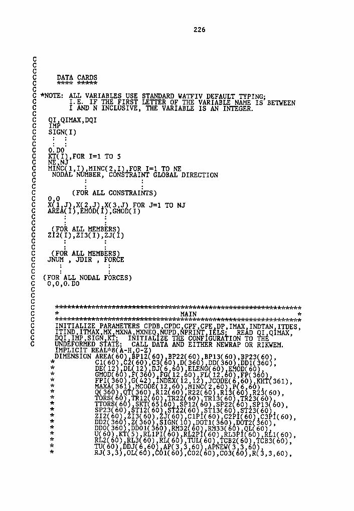
226
CCCC DATA CARDSQC
C *NOTE: ALL VARIABLES USE STANDARD WATFIV DEFAULT TYPING;C I.E. IF THE FIRST LETTER OF THE VARIABLE NAME IS BETWEENg I AND N INCLUSIVE, THE VARIABLE IS AN INTEGER.
8 Qä§QIMAX,DQISIGN(I)
c E EC 0.DOC KT(I),FOR I=1 TO 5
NINUJI I MINC(2 I) FOR I 1 TO NEg NODAL,NUMBER, CÖNSTRAINT—GLOBAL DIRECTION
0 E E0 0 (FOR ALL CONSTRAINTS)
C X(1 J X(2 J X(3,J FOR J=1 TO NJ
EAREA(}5,EM00(i),0M06(1)
c E EC (FOR ALL MMBERS}c E EC (FOR ALL MEMBERS)g JNUM , JDIR , FORCE
c E EC (FOR ALL NODAL FORCES)C 0,0,0.D0CCCQC
INITIALIZE PARAMETERS CPDB,CPDC,CPF,CPE DP,IMAX INDTAN ITDES,C ITIND,ITMAX,MX MXNA,MXNEQ NUPD NPRINT IELS• READ
QäQIMAX,2 2222222222222222 2222222222 R E?¥äS”§2?Jé2§E3IMPLICITREAL*8(A-H
O-ZDIMENSIONAREA(60 BP12(60 BP22 60 BP13(60 ,BP23 60 ,* C1ä60g,O2€60g,C3{60) D(360g DD(360ä DD1(g60g,?$2*
Q(360) Q;(360 ,R12(60)’R22(60) R13(60é R$ä(60),* TORS(6Ög TR12 60),TR22(60€,TR13(60€,T 23(602,* TTORS(6 ) SKT 65160% SP12 60%,SP22 60% SPl3 60),* SP23(60) STl2 60% S 22(60g S 13(60g S 23(60g# ZI2 60) 2I3(60), J(60) Cl I(60),C2 I(60 cs I(60),* DD2 360 ,Z(360 ,SIGN(1Ö2,DOT1(360) DOT2 360),* DD0 360 DD01(3602,RM32 60) RM33(6Ög QL 60g* U(60) K (5) RL1PI 60) RL2P (60) RL3 I(60% L1(60),* RL2(6Ö) RLs(60) RL(60) TUL(60g,TCB2(60) CB3(60),* TU€60) DDJ§6 605 Ap(6 5 602,A NEw(6,s 60)* RJ 3,3),OL 6Ö),CÖ1(60),CO2 60),CO3(60),R(3,3,60),
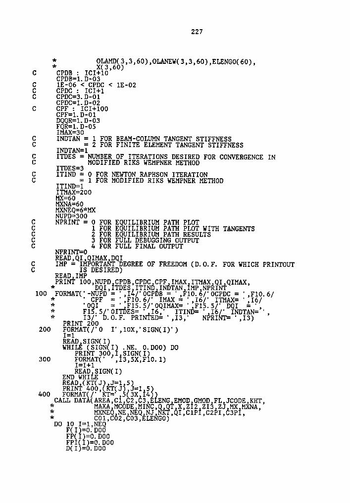
227
* OLAME(3,3,60),0LANEW(3,3,60) ELENGO(60* x(5,6o)
’ )’C CPDB : ICI+10
CPDB=1.D-O3C 1E-06 < CPDC < 1E-02C CPDC : ICI+lC CPDC=3.D-01
CPDC=1.D-02C CPF : ICI+l00
CPF=1.D—01DQQR=1.D-03
¥3§§lsB’°5C INDTAN = 1 FOR BEAM-COLUMN TANGENT STIFFNESSC INDTAN T 2 FOR FINITE ELEMENT TANGENT STIFFNESSC ITDES = NUMBER OF ITERATIONS DESIRED FOR CONVERGENCE INC ITDES 3 MODIFIED RIKS WEMPNER METHODC ITIND = O FOR NEWTON RAPHSON ITERATIONC = 1 FOR MODIFIED RIKS WEMPNER METHOD
ITIND=1ITMAX=200MX=60MXNA=6OMXNEQ=6*MENUPD=300
C NPRINT = 0 FOR EQUILIBRIUM PATH PLOTC 1 FOR EQUILIBRIUM PATH PLOT WITH TANGENTSC 2 FOR ESUILIBRIUM PATH RESULTSC 3 FOR F LL DEBUGGING OUTPUTC 4 FOR FULL FINAL OUTPUT
HEHD QIOQIMAX DQI) 9 9C IMP = IMPORTANT DEGREE OF FREEDOM (D.0.F. FOR WHICH PRINTOUTC IS DESIRED)
READ IMPPRINT 100,NUPD CPDB,CPDC CPF IMAX ITMAX QI QIMAX,
* DQI,ITDES ITIND INDTAN IMP,NPRINT100 FORMAT('-NUPD = ',I4/'OCPDB = ',F10.6/'OCPDC = ',F10.6/
* ' CPF = ',F10.6/' IMAX = ',I6é' ITMAX= ',I6/* '02I = ' F15.S/'0QIMAX= ' F1 .5/' DQI = ',* F1 .56'0ITDES= ' I6,' ITIND= ' I6é%_INDTAN= ',* I3/' .O.F. PRINTED= ',I3,' NPRI - ',I3)
PRINT 200200 FORMAT(/'0 I',l0X,'SIGN(I)')
READ SIGN(I2WHILE (SIGN I} .NE. 0.D00) DO
PRINT 300) SIGN(I)300 FORMAT(' ,I3,5X,F10.1)
I=I+1READ SIGN(I)
J 1 5)PRINT 400,(HT(Jé J=1 5400 FORMATÄ/' KT=' (3X I4 EECALL DAT (AREA,C1 C2,C3, NG EMOD GMOD FL JCODE KHT,
* MAxA Mcövz 215 25 Mx MXMA,* Mxuzé NE NEQ MJ, ,ÖI,C1PI,C2PI,C3PI,* C01,CÖ2,C03,ELENGO)
DO 10 I=1,NEQF(I}=0.DOOFP( %=0.D00FPI( )=0.D00D(I)=0.D00
228
DD(I)=0.D00DDO( )=0.D0Z(I&§0.D00
10 CONTIN
C IELS=0C INITIALIZE THE NODAL ORIENTATION MATRIX AT TIME 0 TOC IDENTITY MATRIX.
DO 35 J=1 NJDO 88 8811313QIF ÄK .EQ. L) THEN DOELSEP£§,L,J)=1.D0
AP(K,L,J)=0.D0END IF
20 CONTINUE30 CONTINUE
C 35 CONTINUEC CALCULATE THE COMPONENTS OF THE INITIAL ORIENTATION MATRIX
° 88 888888%O£iäg=(C0l(I)**2+C03(I)**2)**0.5O 1,1,I =C01 I
88% 8*8*8 :8888Q Q
88288 888 Z6888’*°°2“"°L"’
Q QOLAMD 2,3,I =—C02gIg*C03(I)/OL(I)
88288 8288 :8*88 I ’°8“’Q Q °OLAMD 3,3,I =C0l(I)/OL(I)
C 40 CONTINUEIF (ITIND .EQ. OÄETHEN DO
CALL NEWRAP(A A BP12 BP22 BP13 BP23 Cl C2 C3,D,DD DDl,1 00 0L0u0 0u00,0u00 0 00 0L FP,FPI 0 100001 MAXA,MCODEi$T R12 R22 R1s R23,TORS,TRl2,TR22,* TR13,TR23, ORS SÜT SP12 8P22 SPl3 SP23,ST12,1 ST22 STI3 s12s 212 2I3,ZJ 0000,0000 001,1 101 IELS 1uAx 11uA2,N0,N00 NJ,NKT,NÜPD,* 0,01 ClPI,C2PI,C3PI QIMAX,D¥I,DJ MINC,* R TIND Rusz Russ QL TU IND AN,K1 IMP1 NPRINT 01 RL1PI RLZPI RL3PI RL1 RL2 RL3 RL,* TUL,TC82,TCB3 001 A0,APu0w,äJ 0L 001 002* C03,DL,R,OLAMD,OLÄNEW,DQQR,FQR,ELENGÖ,DDO)ELS§ID8 DO
ALL RIKWEM(AREA BP12 BP22 BP13 BP23 Cl C2 C3,D,DD DDl1 00 0L0u0 Lu00,0u00 0 FG,FL FP,FPI 0 J0000,’* MAXA,MCOÖE QT R12 R22 R13 R2s,10Ré,1R12,1 TR22,TRl3,TR28,TTÖRS SKT,8Pl2 spzz SPl31 SP23,STl2 ST22 STl3,ST23 z12,21s,z1,0R00,* CPDC,CPF,ICI IELS IMAX ITMAX,NE NEQ NJ,« NKT NUPD,Q Q1 C1PI,C2PI,C3PI 002 z SIGN,1 ITDES QIMAX DÖI,DJ,MINC R DOT1,DÖT2 111u01 000 DÖOI RM82 RM33 QL,TÜ INDTAN KT iup NPRINT1 RLIPI RL2PI,RL3PI RL1 RL2 RLs RL 10L TÖB2,TCB8,1 DDJ,AP,APNEW RJ,0L 001 C02,C08,DL,R,ÖLAMD,* OLANEW 0QQR FQR ELENGO)Q Q Q
END IFSTOPEND
CC

229
************«*«*************«**************************«*«*HRR* R*****«******************«***«**2é;é************«*«*«**«*******SUBROUTINE DATA(AREA,C1 C2 C3 ELENG,EMOD,GMOD FL JCODE,
* KHT,MAXA,MCODE MINC,3éQT,X,ZI2,ZI3,* ZJ§MXÖMXNAéMMNEQÖNEÖ QéNJ,NKT,8I* C1 I 2PI, 3PI,C 1 02, 03 ELEN gg
g ägäg NE,NJ; IF NE .LE. MX AND NJ .LE. MX, CALL S UCT AND
IMPLICIT REAL*8(A-H O-Z)DIMENSION AREAä1g,CI(1€ C2(12 C3(1) ELENG(1)
* EN00 1 ,0NoD 1),FL iz 1) JCODE(6 15* KHT(1) MAXA(1),MCODE(12 ig MINC(2 15* 311} QT(l) X§3 lg 212115 I3(1) 25115,* IP (1) CZPI 15 3PI(1),Ö01(l),C02 1 ,*READ NE NJC03(1),ELENGO(1)
PRINT 100,NE NJ100
TgR?ÜE(LEE
Ex ’A§07XN0NJL; |MX§)THEN 001*
C1PI,C2PI C3PI;COI C02,Ö03,ELENGO)’
CALL L0A0101 C2,Ö3 ELENG,EMOD 0N0¤,PL,5000E,* MCÖDE,Q,ÖT,ZI2,ZI3,ZJ,MXNA,NE,NEQ,QI)
ELSE DOPRINT 200200 §¥ägAT('-***NE OR NJ EXCEDES MK; REDIMENSION ARRAYS')
ä§D IFEND
CC
*2******R*******************************«****«**«***«****«****E;=':¤'¤’¢·k·k·k¤'n\··lr·k7'¢1':in'r=':='¢v'r='c='¤'c*v’:¤'¢iri¤':*•!c·!r=§r§*§§’g=(;::;ir='r='r:'c·k·k2’:·Jr='r·!¢v'r='¢=':=’:1'::'r1':v':v':=':=':v'::'::'c:'¢v'rSUBROUTINE STRUCT(AREA,ELENG,EMOD GMOD,JCODE,KHT,MAXA MCODE,
* MINC,X ZI2 ZI3,ZJ,MXNEQ NE,Näg,NJ NRT,« C1PI,C2PI C3PI 001 002 Ö03,E NGOÄ0 READ AND E0H0, MINC· INITIALIZE THE ELEMENTS OF J00 EC TO UNITY· FOR EACH NODAL CONSTRAINT,READ AND ECHO, JNÜM,JDIR,C AND STORE A ZERO IN THE CORRESPONDING LOCATION OF JCODE;
DIMENSION AREA(1),ELENG21g EMOD(1) GMOD(12 JCODEE6,1 ,* KHT 1 ,MAXA(1) CODE(12 I) MINC 2 1) X 3 1 ,* 212 1 ,213 1g,ZJ(1) 01PT115 C2PI(I),C3PI(1 ,* 001 1 ,002 1 003115,ELEN00(1)
READ (MINC(1,I),MINC 2,I),I=1,NE)PRINT 100 _ _ _100 FORMAT(/ - ,7X, MINC )
DO 10 I=1 2PRINT 200,(MINC(I J; J=1,NE)
200 FORMAT('0 ,22(2X,I4 510 CONTINUE*’°
88 23*1**2 6J000E1T J)=120 00NTINuE’
30 CONTINUEPRINT 300 „
300 FORMAT( '-' 10X,'NODAL NUMBER',l0X,'CONSTRAINT DIRECTION')READ,JN{IM,JDIR
230
WHILE (JNUM .NE. 0) DOPRINT 400?JNUM,JDIR
400 FORMAT('0 ,1lX,I4 24X,I2)JCODE(JDIR JNUM)=ÖREAD JNuM,301R
C END wuxizCALL CODES(JCODE,MCODE MINC,MMNEQ,NE NEQ,NJ)CALL DETMAX(KHT MAXA,MCODE NE NEQ,NKT)CALL PROP(AREA ELENG,EMOD,ÖMOD,MINC X ZI2 ZI3 ZJ
* NE,NJ,C1PI,C2PI,C3PI,C0l,Ö02,C03,ELENGÖ)RETURNEND
C
8c *****************************«**********«***«****«**«***««**«*
* *g 7'c·J:='¤‘¢·k1cidnh'c~J\•1':i¤hgc=(2vI'2=§§¤':¤%fricv’¢ic1'¢=%i:¤¥1c=':·!n'¢·!¢='¢·kv\·1’c='c1'<=':=F¢i¢:'¢=‘:=kSUBROUTINE CODESÄJCODE,MCODE,MINC MXNEQ NE,NE3 NJ)
C GENERATE JCODE; ND GENERATE MCODE, BY ÜSING INC AND JCODE.IMPLICIT REAL*8EA-H O-Z5£éäE§SION JCODE 6,1),MC DE(12,1),MINC(2,1)
DO 20 J=1 NJ00 10 L=1 6IF (JCÖDE(L J) .NE. 0) THEN DO
NEQ=NEQ+1JCODE(L,J)=NEQ
END IF10 CONTINUE20 CONTINUE
IF (NE3T.GT. MXNEQ) THEN DOPRI 100
100 §$ggAT('- *** NEQ EXCEDES MMNEQ ; REDIMENSION ARRAYS ***')END IFPRINT 200
200 FORMAT(/'-',7X,'JCODE')DO 30 I=1 6
PRINT 300)(JCODE(I Jg,J=1,NJ)300 FORMAT('0 ,22(2X,I4)
30 CONTINUEDO 50 I=1 NEJ=MINCE1,Ig
K=MINC 2 I00 ao L=i 6MCODE€L,I)=JCODE(L J)MCODE L+6,I)=JCODE(L,K)
40 CONTINUE50 CONTINUE
PRINT 400400 FORMAT(/'-' 7X,'MCODE')00 60 1=1 1é
PRINT 500}(MCODE(I Jg,J=1,NE)500 FORMAT('0 ,22(2X,I4)
60 CONTINUERETURNEND
C
SC *«**«***w****«*****«************«*******w*******«**««**w******C * DETMAX *C fr=’:1':·!c1'c1'r·!r1%='¢·)¢='¢¤’¢v'¢1':ic7'¢·1'r='n'¢:'¤'c7'd:v'¤'n'c:'¢1'c1Vc·J¢1'::'¢2%='r=':='r:'Hc1'cin'¢v'r=':='¢9n'¢**i<icv'r·!¢7’rici:=kirv¥ic=’¢='r1r
SUBROUTINE DETMAX(KHT,MAXA,MCODE,NE,NEQ,NKT)
231
C CALCULATE COLUMN HEIGHTS KHT; AND CALCULATE ADDRESSES OFC DIAGONAL ELEMENTS IN BANDED MATRIX WHOSE COLUMN HEIGHTSC ARE KNOWN MAXA.
IMPLICIT REAL*8(A-H 0-2)DIMNSION KHT(1),MAXA(1 ,MCODE(12,1)DO 10 I=1,NEQ
KHT(I)=010 CONTINUEDO 301I=1,NE
WHILE( MCODE(J,I) .EQ. 0) DOJ=J+1
END WHILEMIN=MCODE(J,I)J=J+1DO 20 L=J 12‘§§”€,C2CC,%-„%· C2, mm ,0
KHTÄK)¥MAXO(KHT(K),(K-MIN))END IF
20 CONTINUECC %3¥”§%”‘£ä¤100 FORMAT(//'-' SX 'I' 10X 'KHT(I ' 10X °MAXA II I I I ) I I ( 9 )
DO 40 =1 NEQPRINT 200,1 KHT(Ig MAXA(I&
200 FORMAT('0 ,1X IS X IS 11 ,IS)MAXA(I+1)=MAXÄ(I)+KÜT(I)+1
40 CONTINUENKT=MAXA(NEQ+1)-1
I MAXA(I NKT600 F0RMAT('0C,iX,I5,2gX,I5//1X,'NKT = ·,1s)
RETURNEND
8Cg *****«******«**««**«***«*****«A«*««*A*««**«******«*««*«***«***A .
friririrvkirfcfdcivvkicirfciricicüicicidriciric1'd¤'r·lv·:'¢7':£§9¢=€=’:='cz·'c1‘:·!:·»'c=k1'cv'c·Ir1'¢ici¢1'r¤'cv'¢*='c='c='c1'c·l¢v'cs'c='cv':;
c READ AND Ecuo THE NODAL COÖRDINÄTES ’x(1fa& ’AND’ELzMEN%C PROPERTIES. FOR EACH ELEMENT COMPUTE THE I ITIAL ELEMENT
CDIMENSION AREA(1) ELENG21) EMOD(12 GMOD(12 MINC(2 1),* x($ 1) 2I2(l) z $(1) za ig ClPI ig C2PI(1 ,* C3PIä1) COIEI) C02(l),C03 1),ELEN 6(1)
!1§ä=§>d_(?fgä,J),X 2,3) ,X 3,—)),J=1,NJ)100*FORMAT({6g-QXQOLOBAL NODAL COORDINATES',/,18x,'x1·,10x,·Xg·,
DOJ (X(I J I 1 3)
NODE >:I3,3(2X,F10.4))PRINT 300
300 FORMAT([é'-' 'ELEMENT PROPERTIES'/ 9X,'N0.',9X,'AREA',10X,* LENÖ',12X,'EMOD',12X,'GMOD')
DO 20 I=1 NEJ=MINC£l,IgK=MINC 2 IEL1=X(1,X)—X(1,J)

232
EL2=X£2,K)-X22,JEL3=X 3 K -X 3 JELENGO(I)=DS3RTE L1**2+EL2**2+EL3**2)ELENG(Ig=ELE GO ICOl I = L1/ELENG0 ICO2 I =EL2/ELENG0 IC03 I =EL3/ELENG0 ISääägxääääßäC3PI I =C03 IREAD A A(I) MOD(I GMOD IPRINT 400,1 AREA(I£?ELENG§I) EMOD(I GMOD(1)
438 C0N¥?§gäT('0,6X,I4,7 ,F8.3,3(2X,D15.7 )
CPRINT 410
410 ä8Rä§g({£i'Né,8X,'NO.',l2X,'ZI2',18X,'ZI3',17X,'ZJ')
READ ZI2(I ZI3 I ,ZJ(IPRINT 420,I:ZI2§1) ZI3(I),ZJ(I)
420 FORMAT(' ,6X,I ,3X,D15. ,8X,D15.7,6X,D15.7)430 CONTINUE
RETURNC ENDCCg
«**************************«*******************«*«*****«******« R
SUBROUTINE LOAD(Cl C2,C3 ELENG,EMOD GMOD,FL,JCODE,
i gggDäiQ,0T,ZI2,ZI3,ZJ,MXNA,NE,
E ä§é¥IALIZE THE NODAL LOAD VECTOR,Q,TO ZERO. CALL JLOAD ANDIMPLICIT REAL*8(A—H O-Z)DIMENSION C1 l),C2(1) C3§1) ELENG(12 EMOD(12 GMOD(1),
* FL 12,1% JCODE 6 1g,MCODE 12,1),0 1),* gg 1),Z 2(1),ZI3(1 ,zJ(1)
DO10CONTINUE ·CALL JLOAD(JCODE,Q)RETURN
C ENDC
R*
SUBROUTINE JLOAD(JCODEg¥EAg,ECHO JNUM,JDIR,AND APPLIED FORCE, FORCE; STORE FORCE
IMPLICIT REAL*8§A-H O~Z)DIMENSION JCODE 6 1g,Q(1),QT(1)
DOPRINT Too'100 FORMAT([/'-' 3X,'NODAL NUMBER',10X,'GLOBAL DIRECT1ON',10X,
*END IF APPLIED FORCE')WHILE (JNUM .NE. 0) DO —
PRINT 200,JNUM JDIR FORCE200 FORMAT('O 6X I4,22X,I2,13X,F16.5,/)K=JCODE(JDIR,JNUM)
233
Q( §1))=FORCERE JNUM,JD1R,E0R0EEND WHIDE
RETURNEND
00
·k ic
gSUBROUTINE NEWRAP(AREA BP12 BP22 BPl3 BP23 C1 C2 06,D,DD,DD1,* DE EDENG EMOD,ÖMOD F FG,EL ÜP,ÜPI 0 JCODE,« MAXA,MCODE QT R12 R21 R13 ä23,TOR§,TR12,* TR22,TRl3,TR2$,TTÖRS éKT,éP12 spzz sR16« sP26,sT12 sT22 STl3,§T23 z12,Z16,z5,0pD6,* CPDC,CPF,1CI IELS IMAX ITMAX,NE,NEQ NJ,6 NKT NUPD 0,01 CIP1 CZP1 C3PI,QIMAX,D2I,DJ« MINÖ,P,IT ND,§M32 NM33 QL TU,INDTAN T IMÜ,« NPR1NT RL1P1 RLZP1 RLBÜ ÄLI RL2,RL$,RL* TUL,TCD2,TCBÄ DDJ ÄP,APNEW,Rj OL 001 001« 006,DL R OLAMD OLÄNEW DQQR,F8R EDENGÖ DDÖ)0 EMPLOY NEwT0N—RAPHs0N ITERÄTION ÖR MODIÜIED NE TÖN-RAPHÄON0 TTEREETQNREQLQRRÄVE 3TZ§HE EQUILIBRIUM POINT.
DIMENSION AREA(lß BDl2(1) BP22§1 ,BP13(lg BP23(1) 01(1) C2(1),* C3(l2 (12 DD(1 DD1 1 DE(1) LEN0(1% ÜMOD(1« GMOD 1),E ig FG 12,1g L(12,1 ,FP(l) F1(1§ 0 1 ,# J00DE(6 1) ÄXA 12 M 6DE 12 1 Q(1) ÖT(1) 12 1 ,:: 1 1612 1"RZS111 lg« SPl3 15’SP23 1é,STl2(1 éT22(1ä’sT16(1é’sT26(1 1* ZI2(1) ZI3(l) 1(1g 0161(é& C2 1(1g C3 1(1E* DJ 6 1éTM1N0(1 1) (6 1) 62(1g R 66(1& Q (1),* TU 15 (1 RL1P (1) §L2ÖI(1) R $R1(1g Ll(l),* RL2(15 RL6 1),RL(1 ,1UL(12 TCÜ2(1) TC $(1),« DDJ 6,1) AP(3 6 60 ,APNEW 6 6 60) ÄJ(3,l)* 0%Älg C01(1) éoägé ,006(1) 6L(äg,ä(6,6,605,# 0 M (6,6,605,0 W(3,3,6Ö),E N00(1),
C# DDO(1)
E ääägIALIZE THE TOTAL RELATTVE DEF0RMAT10N or ELEMENT 1 TODO S I=1 NE
TR12 1 =0.D0TR22 I =0.DO
$11 1’8·
B8$1*15 1‘86”°TCB2 =O. DOTCB3(I5=O.D0TU( Ig=0. DO
s CONTINU0NN=1CALL FORCES(AREA,BPl2,BP22,BP13 BP23 Cl 02,06 DD,DE ELEN0
* EMOD,GMOD,F FG,FL M60DE ÖT §12,R2é R13 Ü23 TOÄS,* TR12,TR22,TÄl3,TRé3,TTOÄS éPl2,SP2é,SP13 SÜ23,* STl2,ST22,STl3,ST23,ZI2 Z13 zJ IMAX,NE Näg,#
3QI,ClPI,C2PI 06p1 RM3Ö,RMä3 ÖL,TU INÖT ,ii T6111‘216§L1ä16R1ä§11111’$1111L11¢§1‘6*111*11*
* MINÖ,OL ÖO1 062,066 DL,§ ODAMD,OLANÜW,* DQQR,EQR,ELEN00,NJ,6D0,111ND,NN)CALL UpDATE(Q ,Q,NEQ,Q1)
234
WHILE( I .LE. QIMAX) DONC=N3PD
gUPSNDTHé§Cg0.LE. ITMAX) DOCALL STIFF(ARgA BP12 BP22 BP13 BP23 C1PI CZPI C3PI,
* ELENÖ Eu0Ö 6uoÖ 6 uAxA MÖODE,TR12,TR22,* TR13,TR23,§KT SP12,SP22 SPl3 sp2s,sT12,* ST22,ST13,ST23 ZI2 ZI3,2J,IELS,NE NKT* Rusz RM33 QL TÜ,INDTAN KT NPRINT,RL1PI,* RL2PI,RL3P RLl,RL2,RL3,RL,Cl,C2,C3,« OLAM®,ELENGÖ)
NC=O
CEND IFCALL STORE(RL1PI RLZPI RL3PI,ELENG,RL1,RL2,RL3,RL,
* C1PI,Ö2PI,C3PI C1,C2,C3,NEgCALL SOLVE(DD,F,MAXA,QT,SRT,NC,NEQ,NE PIV,NKT,NPRINT)D° ä?H‘ég&‘%2D¤m
10 CONTINOEIF (ITCT .EQ. 0) THEN DO
DO 20 I=1,NEQDD1(I)=DD(I)
20 CONTINUE
C END IFCALL FORCES(AREA BP12 BP22 BP13 BP23,C1 C2 C3 DD,DE# ELENÖ Eu0Ö 6uoÖ p,pé FL uc0Öp ÖT,Rl2 R22
* R13 R2s TORS TRI2 TR22 TR13 TR23 TTORS,SP12,* SP22,SP13 SP23,ST12,ST22,ST13,ST23,ZI2 zxs,* ZJ IMAX,NE,NEQ Q,QI C1PI,C2PI C3PI RM32« RM33 QL,Tu INDTAN NPRINT RLIPI RLZPI RLsp1,* RL1 RL2,RL3,RL,TUL TCB2,TCB3 ÖÖJ Jc0ÖE* AP Apuzw RJ,MINC 0L,C01,C02 cos ÖL R,0LAMD,« OLÄNEW DÖQR FQR,ELENGO,NJ,DDO TTTNÖ NNgCALL TEST(AREA BP12 BP22 BP13 Bpzs Cl C2,Ö3 Ö ÖÖ Ö 1,DE,* ELENÖ pu0Ö,6u0Ö p pé FL,FP ppx JcÖÖÖ,ué0¤E,* QT R12 R22 R13,R23 TÖRS SPi2,SP22 sp1s# SP23,ST12 §T22,ST13 ST23,ZI2 ZI3,2J cpÖB,* cpmc cpp ICI IMAX,NE,NEQ,NJ,Ö,QI,CI1,CI2,* c1s ITIND NPRINT)IF pRHL§TN’{0bE?TcT) MN DO
100 FORMAT([/;-' 7X,'NEWTON—RAPHSON ITERATION ',I5//10X,* QT' 20X,'F',20X,'D°)DO so 1=1 NEQ
PRINT 200,QTEI§,F(I) D(I)200 FORMAT('0 ,3 5 ,D15.Ü))
30 CONTINUE
C END IFNC=NC+1ITCT=ITCT+1DO 40 I=1,NE?
FPI(I)=F( )40 CONTINUE
END WHILEIF (NPRINT .E?. 3% THEN DOPRINT 300, CI TCT
300 FORMAT(// ICI=',I4,5X,'ITCT=',I4)END IFDO 50 I=1 NEQ
pp(1g=p(1)50 CONTINU

235
CALL RESULT(C1 C2,C3 D DJ ELENG EMOD GMOD FG FL,* JCÖDE Mc6DE MINC,P Q ZI2,ZI3,ZJ,* NE,NEQ,NJ,Q1,1MP,NéR1 5
?I=QI+DQIF (ICI .NE. 0) THEN DO
PRINT 400400 §"?_äb1;AT(' *** LAST SOLUTION IS NOT CONVERGED ***')END IFENDC$§¥LgPDATE(QT„Q,NEQ„QI)
RETURNEND
ccc
CSUBRQUTINE RIKWEM(AREA BP12 BP22 BP13 BP23 C1 cz C3,D,DD DDI,# DE ELENG EM00,éM0D E FG EL 1p,EP1 6 JCODE,* MARA,MCODE QT R12 R21 R13 R23,T0R§,1R12,* TR22,TRl3,TR2Ö,TTÖRS SKT,SPl2 spzz sP13* sP23,sT12 ST22 ST13,ST23 ZI2,ZI3,ZJ,CPDD,* CPDC,CPF,ICI IELS IMAX ITMAX,NE NEQ NJ,* NKT NUPD,Q Q1 C1PI,C2PI,C3PI DDÖ z SIGN,* ITDES QIMAÄ DOI,DJ,MINC P DOTl,DÖTÖ 1T1N0,* 000 DD01 RMÖ2 RM33,QL TÜ,INDTAN KT 1MP,* NPRINT,RL1PI RLZPI RLÖPI RL1,RLÖ,RL3,* RL TUL TCB2,TCB3,DDJ,AP ÄPNEW,RJ 0L,: %8é,g£§ügg3,¤L,R,0LAM0,6LANEw,¤QQR,
1MPL1c1T REAL*8(A-H oiz)«1’1’111"S1°11 88811 186111188% 188% 1;188%S1818§8€11’1$88%1 111 111L
* GMOD21),F€1g FG§L2,lg L§l2,l ,FP(l) gPI(l& cgi),ii $S$811S‘11%z11Xäz%21” $8%% 1 $$2158-11186111 1 1K 1 % K1TR13 1 ,TR23 1 ,TT0 (1 s 1 ,SPl2 1 ,sP22 1 ,* SPl3 1 SP23 1 ST12(1ß ST22 1 ST13 1 ST23 1* ZI2(1) 2I3(l) J(1) Cl I(l),C2 1 1),03 1(1 ,DD2(l),* Z(l) SIGN(1 DJ(6 1 MINC(2 1 ,P 6 1) DOTl 1),* D0T2(1&T¤00 1£,¤¤01 ig RM32(1 RM33ä1 ,QL(l)# TU(l) (12 R 1P1(1) L2PI(1é RLSPI 1 RL1(l$,* RL2 15 RL3 1),RL(1 ,TUL(1) T D2(1) TC 3(1)* 00J 6 1) AP(3,3 60 APNEW(Ö 3 60),RJ(3,1),ÖL(l),* co1 12 CO2(lg,CÖ3(lg ¤L(1) R($ 3,602* OLAMD $,3,60 ,0LANE (3,3,6Ö),ELENGO 1)
ITCT=0
C NEGPIV=0c INITIALIZE THE TOTAL RELATTVE DEEQRMATTQN or ELEMENT 1c TO zERO.
DO 5 I=1 NETR12 1 =o.¤0TR22 I =0.D0TR13 I =0.D0TR23 I =0.D0TTORs( g=O.DOTUL(I}= .D0TCB2§ g=0.DOTCB3 I =O.D0TU(ög=0.D0
C 5 c0NT1NNN=1
236
CALL FORCES(AREA,BP12,BP22,BP13 BP23 C1 C2,C3 DD DE ELENG# EMOD,GMOD,F FG,FL N600E QT §12,R22 R13626rc*
TUL TCL2 TCB3 001 ÜCODE Ap AÜNEW’RJ’ ’
* MIN0,0L 001 662,666 DL,Ä OLAM®,0LANEW,C * DQQR,FQÄ,ELENGO,NJ,DDO,ITIND,NN)
WHILE (QI .LE. QIMAX .AND. ITCT .LE. ITMAX DOCALL STIFF(AREA,BP12,BP22 BPl3 BP23 CIPI C2PI C3PI ELENG,
* EMOD 6N00 6 MAÜA N660E TEIZ TE22 T616 TÄ23,* SKT SP12,SP22 Spis SP23,ST12 ST22 ST134 ST23,ZI2,ZI3,ZJ IELS NE NKT EM32 ÄM33,0L,I T0,1N0TAN KT NPÄINT 6L161 RLZPI äL3PI,
RL RL2 RL3,ÄL Cl,C2 C3,0LAMD ELENGO&CALL STORE(RL1FI RLZPI RL3PI,ELENG,RL1,RL2,RL3, L,* ClPI,C2PI C3PI C1,C2,C3,NE)
CALL SOLVE(DDOl Z MAXA Q,SKT,0,NEQ,NEGPIV,NKT,NPRINT)IF
DDO1 NEQ)+l DO)ELSE 00’ ’ '
D$I=SIGN(NEGPIV+1 *DSéDSQRT(DOTPRD(DD01,DD0l,NEQ)+1.DO)I (NPRINT .EQ. 3 TH N DO
250 £äé§XTä50,SIGN NEGPIV+1g,NEGPIV§DSiDQI _ __[/ SIGN- D15. , NEG IV- ,I4/ DS- ,Dl5.7,
* DQI=',D1$.7)END IF
END IF
B8L1äL?LE NEDDO(IgéDQ?*DDO1(I)D(I&; (I)+DDO(I)
10 CONTIN
?%’?N$§?NE EQ E THEN DOPRINT 496,01 DQIMP) _ _400 ENDF?§MAT( ,2ÖX,F13.7/ ,20X,F14.8)
IF (NPRINT .EQ. 32 THEN DO
500 ' F13 7 ' D INIT ' ' F14 8Ä Q S ° S — S'C
NN=1CALL FORCES(AREA,BP12,BP22,BP13 BP23 C1 C2,C3 DD DE ELENG,# EN00,6N00,¥,E6,EL,u600E ÖT N12,R22 R13 626
i#NEQ O,QI C1PI,C2PI CBPI §M32’RM33 0L
TU,’ ’
* INDTAN,NÜRINT RLIPI RLZFI RL3PI RLl,§L2,RL3,# RL,TuL TCB2,TCB3 003 JCODE AP AFNEW RJ,4 MINC,0L 601 602,606 6L,R OLAMD,OLANEW,* ICI_1
DQQR,FQÄ,ELENGO,NJ,DDO,ITIND,NN)¥%’äLLL
C LLLXL LLIF (NC .6E. 069é E 0
ELLLL*TR13,TR23,SKT SFl2,SP22 SP13,SP23:ST12:
* ST22,ST13,ST2$,ZI2,ZI3,ZJ,IELS,NE,NKT,
237
* RM32 RM33 OL TU,INDTAN KT NPRINT,RLlPI,R RLZPI RL3P RL1 RL2 RL3 RL Cl C2 C3D D D D D D D DR NC O OLAMD,ELENGÖ)END IFCALL STORE(RL1PI RLZPI RL3PI,ELENG,RL1,RL2,RL3,RL,
* C1PI CZPI C3PI C1,C2,C3,NEgCALL SOLVE€DD1,Z,MAXÄ,Q SKT N0,NEQ,NE PIV,NKT,NPRINTCALL SOLVE DD2 F,MAXA,gT SKT 1 NEQ NEGPIV NKT NPRINTDD2 N Q))/(DOTPRDFDDO DDI NE 1=- D D D D 1
DD(I)=D?I*DD1(I)+DD2(I)
20CNN=2CALL FORCES(AREA BP12 BP22 BP13 BP23,Cl C2 C3 DD,DER ELENÖ EMOÖ 0MoD 1,16 FL M006E 61,R12 R22R R13 R23,TORS TRI2 TR22 TR13 TR23 TTORS,SP12,R SP22 6R16 SP23,STI2 6122 6116 6126 212,R 216 21 IMÄX NE NEQ,Ö QI ÖIPI ÖZPI ÖSPI RM32,R RM3Ö QL,TU INDTAN NPRINT RLIPI RL2PI RLBPI,R RL1 RL2 RL3,RL TUL TCB2 TCB3,DDJ JCODE AP,R ARN2w,R1 MINC ÖL CÖl 002 006 DL R,OLAMD,RI QI+DQI 0LANEw,D6QR,16R,LLEN60,N1,DD6,111ND,NN)
8ALL TEST(AREA BP12 BP22 BP13 BP23 C1 C2,C3 D DD DD1,DE,R ELENÖ EM06,0M06 F Fé FL,FP FPI JCÖDE MÖODER QT R12 R22 Rl3,R23 TORS,SPi2 SP22 SPI3 SPZÖ,R ST12 ST22,ST13 ST23,ZI2 216,21 0RDD,0p6c,R CPF,ICI IMAX NE,NEQ,NJ,Ö,QI,CII,CI2,CI3,R ITIND,NPRINT)¥¥‘ä’%I}IF (NPRINT .EQ. 3) THEN DO
PRINT600FORMAT(é/ I ERATION ' I3,' QI=',F13.7,‘ D= ',
* 13.7,' ICI=',I5)END IF
END WHILEITCT=ITCT+1DO 50 I=1 NEQ
FP(ég=F(I)50 CONTINIF §»ä¥§¥I¥00F?2 FI IIIFF I’°
700 FORMAT(//F ',I5,' ITERATIONS')END IFCALL RESULT(C1 C2,C3,D,DJ ELENG EMOD GMOD,FG,FL,JCODE,R MCÖDE MINC P O,QT,ZI2,ZI$,ZJ,NE,NEQ,NJ,R QI IMP NPRINT)IF (101 .NE. 05 THEN D0
PRINT 800800 FORMAT(' *** LAST SOLUTION IS NOT CONVERGED ***')0N0F}E?F
DS=DS*DS3RT(DFLOAT(ITDESS/DFLOAT(IT))IF (NPRI T .EQ. 3) THEN O
PRINT 350,DS350 FORMAT(// DS= ',F14.8,' ***')END IF
END WHILERETURNEND
CC

238
CC **************************«**********************6***%********C *C ********«****#***************«ä£l£§****«***«**«w*****«*««***w;SUBROUTINE STIFF(AREA BP12 BPZZ BP13 BP23 C1PI CZPI C3PI
* ELENG auob cmob 6 MAxA MCODE,TR1Z,TRZ2,TRl3,2:*
TU INDTAN KT,NPRINT RLIPI RLZPI RL3PI:’
* RL1,RLZ,RL3 äL C1 c2 C3,0LAMD,ELENGO)C INITIALIZE THE SYSTEM TANGENT STIFFNESS MATRIX SKT TO ZERO;C FOR EACH ELEMENT CALL ELEMS1 (BEAM-COLUM MODEL) oä ELEMSZC (FINITE ELEMENT MODEL) AND ASSEMS.
IMPLICIT REAL*8(A-H§O·Z)DIMENSION AREA 1 ,B BP13(1) BP23(l) ClPI(l),
1ZZääélä éääélä $$1%%% S§1ä€1§·§¥ä?€%’z§?1§“’· '* RM22115’RM22§1 :QL(1) 1ü(1 KT(12 RL1PI(l) RLZPI(1),* RL3PI(1éÄRLl 1 ,RLZ(léERL3 1),RL 1),C1(1),Ö2(l),* C3(l),0 MD(3, 60),E NGO 1
IF (NPRINT .EQ. 3) THEN DÖPRINT 100
100 FORMAT(//' STIFF CALLED')END IFDO 10 I=1,NKT
SKT(I)=0.D0010 CONTINUEC
WHILE fl .LE. NE) DOIF INDTAN .EQ. 1 THEN DO
CALL ELEMS1(AREA,BPlZ,BPZZ BP13 BP23 C1 C2 C3 ELENG* EMo¤,cM0¤,c TRI2 TRZ2 TR13 TRZ3 SPIZ SPZ2* SP13,SP23,ST1Z,STZ2 ST13 STZ3 212 ZI3 21,1* END IF
1ELs,NE,RM22,RM22,QL,NPR1NT,K1,0LAM¤,éL6N66)IF (INDTAN .EQ. ZE THEN DO
CALL ELEMS2(AR A,C1 CZ C3 ELENG0 EMOD GMOD,G TR1Z
END IFCALLlASSEMS(G,MAXA,MCODE,SKT,I,NKT,NPRINT)
C END WHILEIF (NPRINT .EQ. 3) THEN DO
PRINT 200200 FORMAT(//'0' 7X 'STIFFNESS MATRIX')
PRINT K=1 NKT)300 r0RMA1(· ,6(5x, 15.75)
END IF
ENDCCg
*************«************«*««*w*«*2*******%****************«*********2%*****fcic·i'¢·l¢*1'dc='c=h'c·I¢1k=’r1‘r='c~Irv'c=§·=]‘;;'§gicvägé=':='¤':=’¢·!r='cv‘c¤\··k1'r7’¢·»':1k='r=':¤'c1'r=':v'r·!:=’:·!¢·1c='cv'::SUBROUTINE ELEMS1(AREA,BP12,BPZZ,BP13 BP23 C1 CZ C3 ELENG
* EM0¤,6M0¤,6 TR12 TRZZ TR13 TRZ3 SPIZ SPZZ,* SP13 SPZ3,ST12,ST2Z,ST13 6122,212 ZI3 2J,* 1 IELS NE,RM22,RM22,QL,N§R1NT,KT,6LAMb,* ELENco5

239
C COMPUTE THE COMPONENTS OF THE ELEMENT TANGENT STIFFNESS MATRIXC FOR THE BEAM-COLUMN MODEL.IMPLICIT REAL*8(A-H O-Z)DIMENSION AREA(1é BR12(1E,BP22(1g BP13(1g BP23(1) Cl(1),« C2(l $(11 EL N6(1) E ÖD(1) 6 ÖD(l) 6(i)* TR12 ig,1R2éE1 ,TR13$l;,TR23£lg,SP12$1 ,SF22 1 ,
* SP13 1 SP23 1 ST12 1 ST22 1 ST13 1 ST23 1 ,E 212112 216(1;, 5(1ä RM32(l),RM33(1),QL 1),KT 1 ,* OLAME 3 3 60 ,ELEN Ö(1)
PI=3.141S92653589Ü93IF THEN DO$122 1 =zI¤0oST13 I =4.D00ST23 I =2.D00Gl2=0. 00
Sääää 383G23=O.DO0
IELS=l·END IF
ELSE DOG12=SPl2 I *TRl2 I +SP22 I *TR22 IG22=SP22 I *TRl2 I +SPl2 I *TR22 IG13=SP13 I *TR13 I +SP23 I *TR23 IG23=SP23 I *TR13 I +SP13 I *TR23 IH=(PI**2·Z 2(I)Eé( REASII; LENG0 I **2g+BP12(I)*(TR12(I}
* +TR22 I IZQII- 22(I )**2+ZI2(I)/ZI3( )** (BP13 I ETRISEI + 23EIg =**END IFBPZS I * TR13 I -TR23 I **2)
CC COMPUTE THE COMPONENTS OF THE CONVENTIONAL LINEAR STIFFNESSC MATRIX IN THE LOCAL COORDINATE.
ETA=GMOD(I?*ZJ(Ig/(EMODII *ZI2(I))GP1=PI**2/ H*ELE G0(I)* 2
=• • 77 «ä§§’ä°éi$GéääZ?§$ää§S8&€ $@1GP4=G12/éH*E G0§I§§GP5=G13/ H*ELENG0 I
GP6=G22/ H*ELENG0 IGP7=G23/ H*ELENG0 IGP8=2.D0 ZI3(Il/ZI2(Lg*(ST13iI)+ST23(II)/ELENG0(I)**2
* +(G13+G23) *2/EE NGO(I) *2*PI**2*GP9=ZI3(Ig/ZI2äI£* ST13(Ig+ST23(I))/ELENGO(I)+(G13**2
* +G13* 23%/ E ENGO(I)* I**2"'H)GP10=ZI3(I)/ I2 I£*(ST13(Ig+ST23(I))/ELENGO(I)+(G23**2
* +Gl3*G23)/ E ENGO(I)* I**2*H)GP11=2.D0*(ST12 I)+ST22( /ELENGO(I)**2+(G12+G22)**2/
·k I ) „:v'r2v'cPIv':=':2·:':GP12=·(ST12(I}+ST22iI)ħE NGO(I)·(G12**2+G12*G22)/
*GP13—(E饧g0I l§¥g;'%* ELENG0 I (G22**2+G12*G22
GP15=ST12 I +G12**2/(PI**2*HGP16=ST22äI$+G12*G224(PI**2*H)
ää}ä‘é%§§Ifäää%$?¥’§1%§§%§iä}äZ·"«ääé$ä’%·¥@"¥*211GP19=ST12( )+G22**2/(PI=*2*H)
CGP20=ZI3(I)/ZI2(I)*ST13(I)+G23**2/(PI**2*H)
C COMPUTE THE COMPONENTS OF THE CONVENTIONAL LINEAR STIFFNESSC MATRIX IN THE GLOBAL COORDINATE.
240
ALPHA=EMOD(1 *Z12(1 ELEN60(16(1)=(C1(1l**2*6P1+2(D0*C1(1g*0LAMD(2,1 1)*6P2
* +2.DO C1(1)*0LAMD(3 1 1 *GP3+0LAM®(2,1,1)**2*GP8* +0LAMD$3 1 1l**2*GP11§*ALPHA6(2)=(C£Ääß=C2(1) 6P1+(C1( 2*OLAMD(2 2,1)+C2(12*
* O 2,1, *6P2+(C1 1€*0LAMD£3 2,1 +C2 1)** OLAMD 3,1,1 *GP3+0LAMD 2 1 1)~OLAMD 2,2,1 *6P8* +OLAMD 3 1 1 *OLAMD(3 2*1g*6Ü11)*ALPH6(3)=(C12§B C3(1}·GP1+(C1(12 0 AMD(2 3,1)+C3(1)*i 8%A„3 §·1·1QjiSä§I3€ä„ä2ä°1^¥?i3121ä$$°ä‘§%i3p3‘ i E 1i +g%§Mß$2L%äÄ)*0LAM0(6,1,1)·6 9+0LAMD(3,1, )*OLAM®(2,1,1)*6(5 =(C1 1Ä*OLAMD(2 2 1 *GP4+C1 1 *0LAMD(3 2 1 *GP5
x)
+82éM $2i%äÄ)*0LAMß(6,2,1)*629+0LAM0(6,i,1)*0LAM¤(2,2,1)*
+“‘6’”i8ä2äħ2L1”?3%6ä1äß?§P§*¥%$é%39ä€ä§£€331‘1§§§äAM313 3 1)+* 6212 JALPÜA
’ ’ ’ ’ ü ’ ’
* 0LAM¤$2’1j1§*6216 *ALPÜA ’ ’G(8)=(CäÄ1g»0LAMD 2 2 1 *GP6+C1$1g*0LAMD(3 2,1)*GP7
* +0 M 2,1,1 *ÖLÄM $3 2 1) G 10+0LAMD(3,1,1)** OLAMD 2 2,1 *GP13 ALPÜA
* +0 M 2,1,1 * 3 3 1)*6 10+0LAMD 3 1,1)** 0LAMD22,6,1ä*6216)*AL2HA
’
if7€+°"°"‘8ä2äߧ§2E°1%Iä122äEä§ä2§°%^¥?iä1?3%äi3£ä§äz§°§°¥S¥l§+
* 6211 =ALPÜA’ ’ ’ ’
G(11)=(C2 1 *C3(1 *6P1+(C2(1 *0LAM®(2 3,1)+C3(I ** 0 M 2,2, *6P2+(C2 1 *OLAM®§3 3,1 +C3 1 ** OLAMD 3,2,1 £*GP3+0LAMD22,2 1)10LAMDä2,3,1g*GP8* +OLAMD 3 2,1 OLAMDQS 3,1)*GÖ11£XALPHG(12)=(c2$§ß~0LAMD 2 1 1g*G24+C2$1g*0 MD(3 1 1}*GPS* +0 2,2,1 *0LAM $6 1 1)*6 9+OLAMD(3,2, )** 0LAM0 2 1,1 *6P12 ·ALPÜA
* 0LAM¤§2’2§1§*6212 *ALPÜA’ ’
7¢
1 1)*6P7« -+0 M 2,2,1 *ÖLÄM 6 1 1) 6 10+0LAMD(3:2 1)** OLAMDEZ 1,1§*GP13 *ALPÜA
,
* 8LAM0§2’2’1 *GPl3 *ALPÜA)’ ’ )
G(17)=(CäÄéß*0LAMD 2 3 1ä*GP6+C2$1g*0LAMD(3 3,1)*GP7* +0 2,2,13*0LÄM $3 3 1)*6 10+OLAMD(3,2,1)** OLAMD 2 6 1 *6216)=AL2H2G(18)=(C3 1 ·=2*6P1+2.D0 C3(1)*0LAMD(2 3 1£*GP2+2.D0*
* C3 1 *OLAMD(3 3L1%*GP3+0LAMD(2,3,1) *2*GP8* +0 M $3 3,1)**2*6 11g*ALPHA
6(19)=(C3$%g'0LAMD(2 1 16*6 4+C3Q1g*0LAMD(3 1 1)*GPS* +0L 1 2,3,1 *ÖLÄM Q3 1 1)*6 9+0LAMD(3,3, )** 0LAM¤ 2 1,1 *GP12 *ALPÜA
6(20)=(CäÄ1ß*0LAMD(2 2 1ä*GP4+c3$1g*0LAMD(3 2 1{*GP5* +0 M 2,3,1g*ÖLÄM $6 2 1)*6 9+0LAMD(3,3, )** 0LAM0 2 2,1 *6P12 ·AÄPÜA
6(21)=(Cä$äg*0LAMD(2 3 1 *6P4+C3$1E*0LAMD(3 3 1)*GPS* +0 (2,6,1)*0 (3,3,1)~G 9+0LAMD(3,3, )*
241
* OLAMDSZ 3,I2*GP12 *ALPHAG(22)=(C3Ääß'0LAMD 2 1 I *GP6+C3i1g*OLAMD(3 1,1)*GP7
gäiéüä) G 10+0LAM®(3,3,I)*G(23)=(C3S1;~0LAM® 2 2!Iä*GP6+C3i1%*0LAMD(3 2,1)*GP7l' G ‘°"GG^”GGG·G·""G(24)=(CäÄ1g=OLAMD 2 3 1i*GP6+C3$1g*0LAM®(3 3,1)*GP7+8 M iätgää) 6 10+OLAMD(3,3,1)*
*G(25)=(g%ä1 +Ää;g§l4+OLAMD(2,1,1)**2*GP15+0LAM®(3,1,1)**2*
G(26)=(CäÄI *C2(1)*GP14+0LAMD(2 1 1)*0LAMD(2,2,1)*GP1S* +0 $3 1 )*OLAMD(3,2 1)*ÖP17)*ALPHA
G(27)=(C1S1ä=C3(I)~GPl4+OLAMD(2 1 1)*OLAMD(2,3,1)*GP15* +0 (3 1 *OLAMD(3 3,I)*ÖP17}*ALPHA
*G(28)=(ég1gElKä%ä§14+OLAMD(2,1,1)**2=GP16+0LAMD(3,1,1)**2*
G(29 = -C1( *C2(1 *GP14+0LAMD(2 1 1 *OLAMD 2,2 1)*GP16*
) g0LAMD23 1 1 *OLAMD(3 2 I)*GF1g)*ALPHÄ’
G(30)=(-C1(I *Ö3(1 *GP14+OLÄMD(2J1 1)*0LAMDg2,3,1)*GP16* +0LAMD 3 1 1 *OLAMD(3 3 I)~GÖ18)*ALPH*G(3l)=(gää1 =Kä;g§14+0LAMD(2,2, )**2*GPl5+0LAMD(3,2,1)**2*
fcG(32)=(C2 1 *C3(1 *GP14+0LAM(2 2 1)*OLAMD(2,3,1)*GP15
* +0 (3*2; %*OLAMD(3(3,1)*ÖPl7l*ALPHAG(33)=(—C2(I)* 2*G 14+OLAMD 2,2,1)**2 GP16+OLAM(3,2,1)**2*
* GP18 ·ALPHA
+G‘G“"$6€ä§Ä§§G§‘Bi8¥;ä§$?%"ä‘G&G+é1»{ä¥9’1ä*1%¥-’1§G·G·”"G*"G*G(36)=(ég3g lX;%;gP14+0LAMD(2,3,1)**2*GP16+OLAMD(3,3,1)**2*
*G(37)=(C1(1 ;:2*g§14+0LAM®(2,1,I)**2*GP19+0LAM®(3,1,1)**2*
G(38)=(g§§? *Cä€1)*GP14+OLAM(2 1 1)*0LAMD(2,2,1)*GP19* +0 (3 1 )*0LAMD(3,2 I)*¢P20)*ALPHAG(39)=(ClÄ1g*C3(I)*GP14+OLAMD(2 1 1)*0LAMD(2,3,1)*GP19
* +0L M $3 1 )*0LAMD(3 3 1§*ÖP20)*ALPHA*G(40)=(g§gé *Xä;ä§14+0LAMD(2,2, )**2*GP19+OLAMD(3,2,1)**2*
+ fc z':G(42)=(C3(1g *2*ÖP14+OLAM®(2,3,1)**2* P19+0LAM®(3,3,I)**2*
* GP20 *ALPHAC
IF (KT(2g .GT. 0) THEN DOG(1)— (1)+RM33ä1;*§2.D0*C1(1)*0LAMD(2 1 1);
* +RM32 1 * ·2.D0*C1( *OLAMDÄ3 1 )* + L(I * -0LAMD(2 1 1E**2-OL MD(3 1 1 **2G(2)=G(2)+gM33§1 *äC2(1{*ÖLÄM (2 1 I)+Cl(I)*O£AMD€2 2 1};« +RM32 15+ -c2( )*OLAMD(3 i )—Cl( )#0LAM¤(ä,2, )* +QL(1)* -OLAMDä2,1,I *OLÄMD£2,2,1* -OLAMD 3 1 I *0LAMD 3 2 I gG(3)=G(3)+RM33 1 * C3(I *0LÄM (2 1,1 +C1(1 0LAMD(2 3 1* +RM32 1 # ·C3( %*OLAMD(3 1 1-c1( )*OLAMD(3,3, )* +QL(1)* -0LAMD% ,1,1 *0LÄMD(2,3,1* G -ODAMD 3,léI *9LAMD 3é3é1
(10)=G(10)+RM33€1 *(2.DO~C ( )~OLAMD(3« +RM32 1 * -2.D0*C2( *0LAMDÄ3 2 )
* +QL(12* —0LAMD(2 2 1Ä**2·0L MD(3,2,1)**2)G(11)=G(l1)+RM33 1)*(C3(I}*ÖLÄM (2 2 I)
* +c2 *OLAMD 2,ä, )* +RM32(I)*(-C3 I *0LAMD 3,2,1* ·C2 1 *0LAMD 3,3,1 )
242
* +QL(1)*(-OLAMD 2,2,1 *OLAMD§2,3,1* -OLAMD 3 2 I *OLAMD 3 3 1 )6( 16)=6( 18)+RM33§1g*22. 110 C3(I{=0LAMD(2 5 1)* +RM32 I *= —2.D0*C3( g*OLAMD§$&§ )
*END IF+QL(I)*(-OLAME(2,3,I **2-O (3,3,1)**2)
C IF (NPRINT .E¥. 32 THEN DOPRINT 100 (G KI) KI=l 42)
100 FORMAT(é/P-) 2X,'G(42g FOR ELE.' 13/5(5X D15.7§/* £5X,Dl5.7g/52 X,D15.7g/5$5X,DlS.Ü;/$(5 ,Dl5.7;/*END IF
5 5X,Dl5.7 /5 SX,D1S.7 /5 SX,D15.7 /2 5X,DlS.7 /)
RETURNEND
CC
*SUBROUTINE ELEMS2(AREA,C1,C2 C3 ELENG0 EMOD GMOD,G TR12
jeELEMENT TANGENT STIFFNESS MATRIX
IMPLICIT REAL*8(A—H,O·Z)•
DIMENSION AREA(1 Cl(1) C2(1) C3(1) ELENGO(l) EMOD(1 GMOD(l* G(12 'I'R12E1g,'1'R22(1é T1213(1),1*R25(1$ 1”u(1)2212(1),)’=~ ZI3 1),2.1 1 ,1<1*(1), L(1),OLAMD(3,3,6Ö)
aäéääääääGGMOD=GMOD(I)EL=ELENGO(I)Z2=ZI2 Iäääzää 1CCl=C1 ICC2=C2 ICC3=C3 I
C T1=T2=T3=T4=T5=T6=T7=T8=T9=T10=0.DOC COMPUTE THE CONTRIBUTION OF THE CONVENTIONAL LINEAR STIFFNESSC MATRIX IN THE LOCAL COORDINATE.
IF (KT(l) .GT. 0) THEN DOT1=T1+E*A6EL ,T2=T2+12. 0='=E*Z3£EL**3T3=T3+6.D0*E*Z3/ L**2T4=T4+l2.D0*E*Z2éEL**3T5=T5-6. D0='=E='=Z2/ L**2T6=T6+GGMOD*ZZJ/ELT7=T7+4.D0*E*Z2/ELT8=T8+2.D0*E*Z2/ELT9=T9+4.D0*E*Z3éEL3/EL
CC COMPUTE THE CONTRIBUTION OF THE INITIAL STRESS (GEOMETRIC)C COORDINATE.
T2=T2+1:2D0*QL(I)/ELT3=T3+QL(I)/10.DOT4=T4+1. 2D0='=QL( I ) /ELT5=T5-QL(I)/l0.D0T7=T7+2.D0*QL(I)*EL/15.D0T8=T8-QL(I)*EL/30.DO
243
T9=T9+2.D0*?Li1£*EL/15.D0E /30.DO
CC COMPUTE THE COMPONENTS OF THE GLOBAL ELEMENT STIFFNESS MATRIX.
G51g=T1*CC1**2+T2*OLAMD(2 1 11**2+T4*OLAMD(3,1,1)**2G 2 =T1*CC1*CC2+T2*0LAMD 2 1 *0LAMD(2,2,1)
* +T4*OLAMD(3 1 IEXO Mb(6 IEG(3)=T1*CC1*CC3+T2*O MDÄ2 1 11*0 (2,3,1)
* +T4*OLAMD(3 1 1l*OL MÖ(3 1)G 4 =T3*OLAMD 2,1,1 OLAMD 3,1,1 +T5*OLAMD 3,1,1 *0LAMD 2,1,1G 5 =T3*OLAMD 2,1,1 *OLAMD 3,2,1 +T5*OLAMD 3,1,1 *OLAMD 2,2,1G 6 =T3*OLAMD 2,1,1 *OLAMD 3,3,1 +T5*OLAMD 3,1,1 *OLAMD 2,3,1G 7 =T3*OLAMD 2,1,1 *OLAMD 3,1,1 +T5*OLAMD 3,1,1 *OLAMD 2,1,1G 8 =T3*OLAMD 2,1,1 *OLAMD 3,2,1 +T5*OLAMD 3,1,1 *OLAMD 2,2,1G 9 =T3*0LAMD 2,1 1 *OLAMD 3,3 1 +T5*OLAMD 3 1 1 *OLAMD 2,3,16 lO§=T1*CC2*·2+T2* LAMD(2 2 11*·2+T4*OLAMD(3,2, )**2G 11 =T1*CC2*CC3+T2*OLAMD 2 2 )*OLAMD(2,3,1)
* +T4*OLAMD(3 2 12*OL b(é 6 1)*G(12)=gä§ggAäD&2i2,1)=OLAMD(3,1,1)+TS*OLAMD(3,2,1)*
*G(13)=gä§ggÄäÖé2i2,1)*OLAMD(3,2,1)+T5*OLAMD(3,2,1)*
*G(14)=gäÄgg2äÜg2i2,1)*OLAMD(3,3,1)+TS*OLAM®(3,2,1)*
*G(1S)=gäXggÄgÖg2i2,1)*OLAM(3,1,1)+T5*OLAMD(3,2,1)*
*G(16)=gäXggi§Ö$2i2,1)*OLAMD(3,2,1)+TS*0LAMD(3,2,1)*
*G(17)=gäXg%§äÖg2i2,1)*OLAME(3,3,1)+T5*OLAMD(3,2,1)*
Gä 18g=T1*=CC3='=*21·T2*OLAMD: 2 E 3 1 )**2+T4*OLAMD§ 3 , 3 , 11**2*G 19 =gäXg%A§Dä2i3,1)*O (3,1,1)+T5*OLAMD 3,3,1 **G(20)=gä§ggħÖg2i§,1)*0LAME(3,2,1)+TS*OLAME(3,3,1)*
G(21)=T3*OLÄMÜ(2 3,1)*OLAME(3,3,1)+TS*OLAMD(3,3,1)** OLAMDÄZ 6 1)*G(22)=gä;gg gÖä2i§,I)*OLAMD(3,1,I)+T5*OLAMD(3,3,1)*
*G(23)=gä§g3ÄgÖ$2i§,1)*OLAMD(3,2,1)+TS*OLAMD(3,3,1)*
*G(24)=gä§gB%äÖg2i§,1)*OLAMD(3,3,I)+T5*OLAMD(3,3,1)*
G2251=T6*CC1**2iT9*OLAMD(3 1 11**2+T7*OLAMD(2,1,I)**2G 26 =T6*CC1*CC2+T9*OLAMEÄ3 1 )*OLAMD(3,2,1)
* +T7*OLAMD(2 111iXO MÖ(2 211gAG(27)=T6*CC1*CC3+T9<O M£Ä3 1 1)*0 ME(3,3,1)
* +T7*OLAMD(2 1 16*0 MÜ(2,3 IlG€281=-T6*CC1**2+11Ö* LAMD(3 1 11* 2+T8*OLAMD(2,1,1)**2G 29 =—T6*CC1*CC2+T10*OLAMD(3 1 1*OLAMD(3,2,1)
* +T6*0LAM¤(2,1 1l*OLAMD(2 2 1G(30)=·T6*CCl*CC3+T10=OLAMD(3 1 11=OLAMD(3,3,1)* +T8*OLAMD(2 1 1)*0LAMD(2 6, )
G231g=T6*CC2**2+T9*ÖLAMD(3 2 11* 2+T7*OLAME(2,2,1)**2
fc*3
32G233g=-T6*CC2**2+11Ö*OLAMD(3 2’11**2+16*0LAM¤(2,2,1)**2G 34 =-T6*CC2*CC3+T10*OLAMD(3 2 1*OLAMD(3,3,1)
* +16*0L2g¤(2 2 1)*OLAMD(2 61 )G 35 =T6*CC3**2+T9*ÖLAMD(3 3,1)*«2+T7*OLAMD(2 3,1)**2G 36 =—T6='=CC3**2+T10*OLAMD( 3,3 1)**2+T8*0LAMD( 2,3 17)t**2G 37 =T6*CC1**2+T9*OLAMD( 3 1 11*='=2+T7*OLAMD( 2, 1, 1)* 2G 38 =T6*CC1*CC2+T9*OLAMDÄg 1 )*OLAMD(3,2,I)
* +T7*OLAMD(2 11IgÄ0L b(2 2,11G(39)=T6*CC1*CC3+19*O MD(3,1,1)*O (3,3,1)
244
* +T7*OLAM(2 1 I)*OLAM(2 3 I)6 2 1 2 , 2 , 1)**2
G 41 =T6*CC2*CC3+T9*OLAMDÄ3 2 )*OLAMD(3,3,I)* +T7*OLAMD(2 2 I)*OL MD(2 3 I)
G(42g=T6*CC3**2+T9*OLAMD(3,3,I)*%2+T7*OLAMD(2,3,1)**2REEND
SCC ********w*******«********«*********************************«**C * w
CSUBROUTINE ASSEMS(G MAXA,MCODE,SKT I,NKT,NPRIN§%C ASSEMBLE THE CONTRIBUTIONS FROM EACH ELEMENT I O THE GLOBALC SYSTEM STIFFNESS MATRIX.
IMPLICIT REAL*8(A-H O-ZgDIMENSION G(12 MAXA(1), CODE(12,1) SKT(l)INTEGER INDEX 12,12)/1 2,3,4 5,6 -1 -2 -3,7,8 9,
* 2,10,11,12,13,14,-2,-10,-11,15,16,17,* 3,11,18,19,20,21,-3,-11,-l8,22,23,24,* 4,12,19,25,26,27,-4,-12,-19,28,29,30,* 5,13,20,26,31,32,-5,-13,-20,29,33,34,
i 6,lg,2%,2Ä,3§,3g,iöé-%4,;21é30§34,36,D D D D
* -2,-10,-11,-12:-13,-14,2,10,1l,-15,-16,-17,* -3,-11 -18 -19,-20,-21 3,11 18 -22,-23,-24,* 7,l5,22,28,29,30,-7,-15,-22,31,38,39,* 8,16,23,29,33,34,-8,-16,-23,38,40,4l,* 9,l7,24,30,34,36,-9,-17,-24,39,41,42/
DO 20 JE=1 12J=MCODE(JE,I)IF (J .NE. 0 THEN DO
DO 10 NE=1 JEN=MCODE(NE,IIF (N .NE. 0 THEN DOK= MAXA€J +J-N
L=INDEX N ,JE)IF (L .GT .2% THEN DOSKT(K)=S (K)+G(L)
ELSE DOSKT(K)=SKT(K)-G(-L)
END IFEND IF
10 CONTINUEEND IF
20 CONTINUEIF (NPRINT .E?. 3&TTHEN DOPRINT 100, ,(S (KI) KI=1 NKT&
100 ENDF?§MAT(// ',7X,'S 1FFNESS F OM ELEMENT ',I3,/6(5X,D1S.7))
RETURNEND
ECCv':C
s'¢s'dc="n"¤'¢·I¤'::v\··I:1'¢1'c:'c='rv'c1'c='v1'c='¢=$c;£2%='v='¢1':1'c¤'c1'¢~;’c=':1'c·J:v‘c=':='n'r:'c·:'c~Jc='c=':=’:=’rv'<='r¤'r1'c1'c1*cCSUBROUTINE STORE(RLlPI RL2PI,RL3PI ELENG,RL1,RL2,RL3,RL,C1PI,
* C2PI C3PI C1 C2 C3,NEgC STORE THE PREVIOUS ITERATIÖN LENGTH AN DIRECTION COSINES OFC ELEMENT IIMPLICIT REAL*8EA-H O-Z}
DIMNSION RL1PI lg RLZP (1) RL3PI(12,ELENG(1) RL1€1g,RL2(1),* RL3(1), L(l),ClP (1),C2PI l),C3PI(1),Cl 1 ,C2(1),
245
C * C3(1)
DO 30 I=1 NERLIPI 1 =RL1 1RLZPI I =RL2 IRL3PI I =RL3 IELENG I =RL(I)Sé$¥§%§?€é§¥§
30 ¤6N¥¥§6EI‘°’ I
RETURNEND
CCCC 66*66666666666666666666*6666*666666666666666666666666666666666
6 .
SUBROUTINE FORCES(AREA BP12 BP22 BP13 BP23,C1 C2 C3 DD,DE6 ELENÖ EMOD cMOD,E,E6 FL MCOÖE 6T,R12 R226 R13 R23 TORS TRl2 TR22 TRI3 TE23 TTORS,SPl2,S S S S S S S
* RM 3 QL TU IND AN N RINT RLIP RL2 I RL PI6 RL1 RL2’RL2,RL TUL TcE2 TCB3,DDJ JCOÖEAp,’
* APNEW,RJ MINC ÖL CÖ1 002 002 DL R,OLAMD,c *FOR EACHELEMENTIMPLICITREAL*8(A-H O-Z) °
DIMENSION AREA(1ß BP12(12 BP22(1g BP13(1g BP23(1g C1(12 C2(1),6 C3§1), Ö(1ä DE 1 ,ELEN $1),EMO (1) 0M0€l),F
1)6 FG 12 Mc0DE 12 1),0T(15 R12 1 R22 i),6 Rl3(l) 3(lg 0 é(1) TRl2(l TR22 ig TRl3(l)i §¥§ä2}§·§¥2§(€%’s¥€%€€%’g¥§§€€"z¥$(1(‘%1ä?ä§(%3a1)6 1) ClÜI(l C2ÖI(1 C3ÖI(l RM32(1) ÖM22(1 ,ÖL(l),’6 605 RL1PI i)ÜRL2E (1% RL3 i(1 RLl(1 ,RL2 1 ,* RL3(1é RL(1) L(1) TC 2(1& TCB3(1g,TUg1) DDJ(6,1),6 JCODE 6 1) AE(3,3 66) APNE (2,2 60 RJ 2 i),6 MINC(2,1;,ÖLSlg CÖ1(1) C0äħg,CÖ3§l) DL(%g,* R(3 3 60 ,0 (3,3,605,0 w(3, ,6Ö),E NGO(1),6 DDO(15
EC GENERATE THE INCREMENTAL NODAL DISPLACEMENT MATRIXC DDJ(IDIR Jg.DO 53 1 6
B9§éäBé?1€}§°2“°IF Jg (SE. gg 1HE§NgO
ITIND EQ 1) THEN DODDJ(IDIR,J)=DDO(N) ' 'ELSE DO
END IF12 CONTINUE
CC CALCULATE THE INCREMENTAL NODAL ROTATIONS AT NODE J.
OME1=AP(1,1 J)*DDJ(4,J)+AP(1,2,J)*DDJ(5,J)* +AP(1 3 J£*DDJ26 J)
OM£2=AP(2 1 J) DDJ( ,J)+AP(2,2,J)*DDJ(5,J)6 +Ap(2 2 J)6DDJ26 J)OM3=AP(3,1,J)=DDJ( ,J)+AP(3,2,J)*DDJ(5,J)
246
C * +AP(3,3,J)*DDJ(6,J)
C YIELD THE COMPONENTS OF THE ROTATION MATRIX OF NODE J.RJ 1,1 =1.D0RJ 1,2 =0ME3RJ 1,3 =-OME2RJ 2,1 =·OME3RJ 2,2 =1.D0RJ 2,3 =OMElRJ 3,1 =OME2RJ 3,2 =—OME1
CRJ 3,3 =1.D0
C FOR EATCH ITERATION EMPLOYING THE LAST NODAL ORIENTATIONC AND ROTATION MATRICES OF NODE J TO GENERATE THE NEWC NODAL ORIENTATION MATRIX.
DO 25 L=l,3DO 20 M=1 3
APNEW(L,M,J)=0.D0DO
AFN§WäL3M J) RJ(L K)*AP(K M J)+APNEW(L M J)3 3 3 3 3 3 318 CONTINUE20 CONTINUE25 CONTINUE
DO 27 L=1 3DO
äF(§=K’3) APNEW(L K J)3 3 326 CONTINUE27 CONTINUE28 CONTINUE
DO 10 I=l,NEQF(äö=0.D0C 10 CONTI E
I=1WHILE EI .LE. NE DOIF NPRINT .E . 3) THEN DO
PRINT 100,100
ENDF?§MAT(/'ELEMENT ',I3)
CALL ELEME(AREA,BPl2,BP22,BP13 BP23 C1,C2 C3,DD DE,ELENG,F FM0D,cM0D,F F6,FL Méooß R12 R22 R13,R23 T0RsF TR12,TR22,TR13,TR23,TTORS SR12,SP22 SP13 SP23F sT12,sT22,sT16,sT26 212 ZI3,ZJ I,IMÄX CIRI CZPI,F c6F1 RM32,RM33 QL,TÜ,INDTAN NPRINT,RL1PI RLZPIF RL3PI,RLl,RL2,RL3 RL,TUL,TCE2 TCB3 DDJ 5é0¤F,AR,* APNEW,RJ MINC OL Ö01 C02 C03 DL R,ÖLAMD,F
I 1+1OLANEW,DÖQR,FÖR,ELENO0,DDO,ITIND,NN)
END WHILERETURNEND
C
SC*
*********««*****«FR*«***FFFFRFRFRFRFFFFFFSUBROUTINE ELEME(AREA BP12 BP22 BPl3 BP23,C1 C2 C3,DD DE,F ELENC Fuob GMOD,F,FÖ FL Mcobz R12 R22F R13 R23 TORS,TRl2 TR22 TRl3 TR23 TTORSF SPI2 SP22 SP13,SP23,STI2 ST22 STI3,ST23,F 212 216,25 I,IMAX,ClPI C2PI C3PI RM32,RM33,F QL Tu INDTÄN NPRINT,RLIPI RLZPI RL3PI,RL1F RL2,RL3,RL,TÜL,TCB2 TcB6 b¤J Jc6¤F AF,ARNRw,F RJ,MINC,OL,C0l,C02,Ö03,DL,R,ÖLAMD,ÖLANEW,
247
* DQSR FSR ELENGO,DD0 ITIND NN)C COMPUTE THE LOCAL I TER AL ELEMENT FORCES EL DUE TO THEC DEFORMATIONS· TRANSFORM THEM TO THE GLOBAL ELEMENT FORCESC FG· AND COMPUTE THE NODAL FORCES F CONTRIBUTED BY ELEMENT I.C SXECUTED FOR EACH ELEMENT,I.
DIMFNSION AREA(1g BEl2(1 BP22(1) BP13(1g BP23(1ß C1(1 ,C2(1),* Cßäl), D(1£ 00 1 ,ELENG£1),EM0 (12 GM0 (1) 1 1)iäägää*
TTORSE1) sp12 1) 6p22 1) SP13(1 SP23 1 6112 1* ST22§1g,STl3é1 ,ST23El ,ZI2(1) 113§1),z3(1 ,C1P1(1),* C2PI 1 C3PI 1 RM32 1 RM33(1?,QL 1 U(6O* RL1PI(%g RL2PI 1) RL3? (1),RLl 1) RL2(l),R 3(1),* RL(1g L(1) TCB2(l) TCB3(l2 TU(1) DDJ§6,l ,* 0000 (6 1) AE(3,3 605 Apuzw 3,3 605 RJ 3 1 ,# M1N0(2,1 ,0%Ä1ß CÖ1(1$ 00ä2§g,063(15 DL(1),* R(3,3 60 ,0 M (3,3,605,0 W(3,3,6Ö),* ELENGÖ(1 DDO(1gIF (NPRINT .E?. 3) THEN D
PRINT 100,100 ENDFO§MAT(' DE FOR ELEMENT',I3)DO 10 J=1 12DE(J)=Ö.D0O
K=MCODE(J,I)IF (K .NE. Oä THEN DOIF (NN .E . 1 .AND. ITIND .EQ. 1) THEN DO
DE(J)=DDO(K)ELSE DO
DE(J)=DD(K)END IF
END IFIF (NPRINT.EQ.32 THEN DO
PRINT 200,DE J)200 FORMAT(5X,D15. )
END IF
C 10 CONTINUE
RL3PI I =ELENG I *C3PI IRL1 I = L1PI I + E 7 ·DE 1RL2 I =RL2PI I +DE 8 ·DE 2RL3 I =RL3PI I +DE 9 ·DE 3
CRL(I)=DSQRT(RL1(I) *2+RL2( )**2+RL3(I)**2)
C1 I =RL1 I /RL IC2 I =RL2 I /RL I
CC3 I =RL3 I /RL I
E gä§ä§§¥EITHE INCREMENTS OF THE LOCAL DISPLACEMENTS OF
D 2 =OLAMD 2 ·DE 1 + 2,2, DE 21 I·‘ I "' I7f
DL(3)=OLAMD(3 1 1)£DE(1)+OLAM®(3,2,I)*DE(2)* +0LAMD(3 3 )¤DE23)
DL(4)=OLAMD(l 1 1)‘DE( )+0LAMD(l,2,I)*DE(5)* +0LAM0(1 3 l“DE26)DL(5)=OLAMD(2 1 1) DE( )+OLAM(2,2,I)*DE(5)« +0LAM0(ä 3 )“DE26)DL(6)=OLAMD(3 1 1)~DE( )+OLAMD(3,2,I)*DE(5)
* +OLAMD(33 )=’=DE(6)DL(7)=OLAMD(1,1,1)“DE(7)+OLAMD(1,2,I)*DE(8)
248
* +OLAME(l 3 I *DE(9)DL(8)=OLAMD(2 1 1%£DE(7g+OLAME(2,2,I)*DE(8)
* +OLAME(2 3 £*DE( )*DL(9)=OgAMD(3§1$1g Qg&7g;OLAMD(3,2,1)*DE(8)*DL(10)=O3AMD£ää1éI$*DEéäO%;OLAM(1,2,I)*DE(11)
DL(11)=OLAMD(2 1 1}£DE(10)+OLAME(2,2,I)*DE(1l)* +OLAMD(2 3 )JDE(12)
*DL(12)=OLAMD(3 1 1%JDE(10)+OLAME(3,2,I) DE(11)=~ +0LAm>(3,3, )*1>1·:(1z)
8 GENERATE THE COMPONENTS OF THE ROTATION MATRIX OFC ELEMENT I R.
R 1,1,1 =1.DOD D
—-
R 2,1,1 =-R(1,2,I)R 2,2,1 =1.D0R 2,3,1 =(DL(10)-DL(4))/2.D0R 3,1,1 =-R$1,3,1g
ä3·ä·1?i*‘¤3·3·%C D D —°
O EACH ITERATION EMPLOYING THE LAST ELEMENT ORIENTATIONE AND ROTATION MATRICES TO GENERATE THE NEW ELEMENTC ORIENTATION MATRIX.DO 1% 51521 3
OLANEW(L J 1)=0.D0DO 30 1<=i 3C0N¥L§§äW(L,J,I)=R(L,K,1)*OLAMD(K,J,I)+OLANEW(L,J,I)
3032 CONTINUE34 CONTINUE
DO 37 L=1 3DO 36 5=1 3OLAMD(L,J,I)=OLANEW(L,J,I)
36 CONTINUE37 CONTINUE
CUL=(ELENGO(I)-RL(I))/ELENGO(I)
CC EMPLOYING THE MINC CODE TO OBTAIN THE ELEMENT DEFORMATIONSC AT BOTH ENDS, A AND B.
L=MINC1,11<=1~11Nc%21i/ 1/ {
”1 = - AP 1 1 L +C01 I OL(I *AP(3 1 L
1 *— ’
1 *R13(1)=fۊ1g$)=98311
*C02§I /0L$I *AP(1 1 i+0L( )*AP(é,1,* * *§‘°°2§*
*9832% @31} §i8$ä3·3·1.l61.111: *°2‘I)9Äé€S*§ E2+(-C02{I{iC03Ä12/ÖL(1 )*AP(3,2,L))/ * +C3(I)*$-C01(1£<C02(Ig/O $1)* P 1 3 L +OL(I)+= p$z 3 )+(-co (1)=c03(I)/ÖL(1 2*APÄ3<3;L)&Rzz(1)=C1(I *$-C03 1% ÖL(I}*AP(1 1 K&+C01(I} O 1)**P 3élä’
* +C2$1 -C03$ /0LE *AP$1,ä, ;+C0l§ /0Lä jAPä , ,* +C3 I§*§·C03 1 OL I *AP 1 3 K +C01 I OL I JAP 323,KRg3(1)=-(c1( ) —C01£ *602 1 /OL£1 ·=AP(1 11 +OL( ) AP( ,1,I 1*9983,%*9832%=·«.+C3(I)*Ä-C0l(1?(—C02(I)/0 $1)* P 1 3 K +_OL(1)* * P(2 3 %+€-C02(1%=C03(I%§ÖL(1 gJAP$3,3,Kg))TORS(I)=2.D0*(OLAMD(3,1, )=(-CO1( )*C02( /OL( *AP 1,1,K

249
* +OL(1)*AP(2 1 K +(—C02(I *C03 I OL(I ** AP 3,1,K )+ÖLÄMDÄ3 2,1)*2-COIEI 4C02(1ä{OL(1)** AP 1 2 K +OL(I&* P(2 2 K)+(-CO2 1g*C03 )/* OL I§?*A (3 2 ))+OLÄMD(3 3 1%* · 01(1)*C02(I)/=·= OL 1 *AP(l 5 1’<)+0L(1)='=A1>Äé 5, )
C * +(· * )/0L( ))* P(3,3,K)))C COMPUTE OTAL RELATIVE DE ORMATIONS OF ELEMENT 1.
¥„‘?’;&I%‘?{s1zTR22 I =R22 Iäéäääääéä §TTORS( )=TORS 1)
C
8 T° THE RE‘*^“"EIF (INDTAN .EQ. lg THEN DO °
CALL BOWCOR(AR A,BP12,BP22,BP13,BP23,ELENG R12,R22 R13 R23,=~ SPl2 spzz s1>15,s1·26,s112,sT22 §Tl3 $1*25 ZIÖ,
j;RM12=EMOD§Ig*g12£1 * ST12(I *TR12€1g+ST22(1g*TR22(1gg/RLä1gRM22=EMOD I *ZI2 I * ST22 I *TR12 1 +ST12 1 *TR22 I /RL I
CRM32(1)=(RM12+RM22 / ELENG0 1)**2)
RM13=EMOD(Ig*Z13(1 * ST13(1 *TR1321;+ST23äI;*TR2321g3/RLä1gRM23=EMOD 1 *Z13 I * ST23 1 *TR13 1 +ST13 I *TR23 1 /RL 1
CRM33(I)=(RM13+RM23 / ELENG0 1)**2)
FL 1 I =EMOD(1 *AREA 1 *(TUL(I)-TCB2(I)-TCB3(1))
CQL€I)=FL(1,I)/ELENGO(Ig
C OR COMPUTE THE LOCAL ELEMENT FORCES DUE TO THE RELATIVEC Eä§gRgäT1ONS BY FINITE ELEMENT MODEL.U(1 =RL(1 -ELENG(1)TU( =TU( (jgfbrE1=TEl(I) T" 'E12=TR12 1E22=TR22 IE13=TR13 1E23=TR23 1A=AREA(IgEiääääjZ2=ZI2 ~Z3=ZI3äIg Qß (él /«( )CCPRINT 38 1 E1 E12 E22c 38 F0RMA1* 251 16 5x sizx 1116.7))RM12=E*A*i4.D0*E12·E22g*E1/60.D0+2.D0*E*Z2*i2.D0*E12+E22g/
* EL+E A*E1*E12/1S. 0+E*A*EL*((12.D0*E12·*2-3.D0*E12* 22* +E22**2l*E12/420.D0+(·3.D0*E12**2+4.D0*E12*E22-3.D0** E22**2)·E22/840.D02-E*A*El*E22660.D0RM22=E*A*(4.D0*E22-E12ß=E1/60.D0+2. 0*E*Z2*i2.D0*E22+E12g/* EL-E~A*E1*E12/60. 0+E*A*EL*((12.D0*E22·-2-3.D0*E12* 22* +E12**2)*E22/420.D0+(-3.D0*E12**2+4.D0*E12*E22-3.D0** E22**2)~E12/840.D0)+E*A*E1*E22615.D0RM13=E*A*(4.DO*E13-E23ß*E1/60.D0+2. 0*E*Z3*(2.D0*E13+E23g/* EL+E*A*E1*E13/15. 0+E*A*EL*((12.D0*E13**2-3.D0*E13* 23* +E23**2)*E13/420.D0+(-3.D0*E13**2+4.DO*E13*E23—3.D0** E23**2)*E23/840.DO)-E*A*E1*E23660.D0RM23=E*A*(4.D0*E23-E13B~E1/60.D0+2. O*E*Z3*$2.D0*E23+E13g/* EL-E=A*E1*E13/60. 0+E*A*EL*((12.D0*E23=*2-3.D0*E13* 23* +E13**2)*E23/420.D0+(-3.D0*E13**2+4.D0*E13*E23-3.D0*
250
* E23**2l*E13é840.D0g+E*A*El*E23 15.DOFL(1,I)=(-E·A)*( 1/EL+( .D0*El3—EZ3 *E13é60.D0* + 4.D0*E23-E13g*E23/60.D0+( .D0* 12-E22)*E12/60.DO* QL(I)_ F; ä.?g*E22-E12 *E22/60.DO)
C END IF ’c COMPUTE THE REMAINING LOCAL ELEMENT FORCES.
FL 2,1 =(RM13+RM23) RL(I}FL 3,1 =-(RM12+RM22 {RL( gFL 4,1 =—GMOD(1)*zJ )*TT RS(1)/RL(1)FL 5,1 =RM12FL 6,1 =RM13FL 7,1 =-FL 1,1FL 8,1 =-FL 2,Iää
261c
’ _F1 1%:15%%%’
IF (NPRINT .EQ. 3 THEN DOPRINT 40,1 RL(%{ RM12 RM22 RM13 RM23 STl2(%% ST22(I%ä
* 6113% ,ST2Ö 1 ,1cB2Ei),1cé6(1) ÖRS(I} 12(1),* TR22 1 TRl3 1 ,TR23 1RL2PI(#RL3F1(N5,RL1 1 ,RL2(1g ÄL3(I) (I),ELEN (1)
40 FORMAT(/' ELEME ' 13, L= ',Dl5.7/i Z ä§ä§??·B䧷?·Z äää?Z·Bää‘¥§6 · 6112; ',D15:7,' 6122; ':DlS:7/ii Z D15 7/6 j 1R12= ::Dl5:7:: TR22= ::D15:77
’ °*
_ TR13= _,D15.7,_ TR23= _,D15.7/_ _* RL1PI= ,D15.7, RL2P1= ,D15.7, RL3PI= ,D15.7/i Z R%~ä’Z·B䧷§·Z EL§ä1é’Z·3䧷ä;$
“”"·”‘5·’“PRINT so
_ ’ ' ’ _ ’ '50 FORMAT ' LOCAL ELEMENT FORcES'
PRINT é0,FL§1,Ig,FL§2,I ,FLä3,I§,FL§4 1) FL(5 1) FL(6 1),* FL 7,1 FL 6 1 ,FL 9,1 FL 16, 5 FL(il 1) FL(12,1)60 FORMAT(5X D15.7,5X D15. ,5X D15.7/5x D15.7,5X Di5.Ü,5X6 DI5.7/SX,D15.7,SX,D15.7,SX,Dl5.7/SX,Dl5.7,SX,Dl5.7,*END IF 5X,D15.7/)
cc TRANSFORM TO THE GLOBAL ELEMENT FORCES.
FG(1,I)=C1(I)*FL(l,I)+0LAMD 2,1,1 *FL 2,1* +0LAMD 3,1,1 *FL 3,1*FG(2,I)=C2(I)*FL(1,I)i8%ääB §,ä,1 ig? 2,1
äiäiä $$1%;%:%f°"‘·”“‘“”’Z”""·”I8ä%äiäiä "‘§}: 2:%ic«“"’·”‘°2""'“"*·”i8%3 äiäiä Ziää 2;}äiäzä "§¥: 2;%
:'c*FG(7,I)=Cl(I)*FL(7,I)I8ä2gB §i1i1 jää 3iI*FG(8,I)=C2(I)*FL(7,1):8%% giggggsG<9·I>=¤3<1>*“<7·I>:61—111262% :16 2%FG(l0 1 =C1(I *FL(1O 1 +OLAMD(2,l 1 6FL(11 1)6 ’ )
+0LAÄ(6,1,1)5FL(12,1)’’ ) ’
251
- R„fG‘“·”Ti䥄ä2„%"%‘ä°1§l§€%§’§”&§·2·"*FL‘“·”FG(12,I)=C3(I§*FL(lÖ l+OLAMD( ,3,I)*FL(11,I)
C * +0 (3,3,I) FL(12,I)
DO 80 J=1 12K=MCODE(J,I)IF (K .NE. 0) THEN DO
F(K)=F(K§¥FG(J,I)IF (NPRI .EQ. 3) THEN DO
PRINT 70,F(K&70 FORMAT(' F( )= ',D15.7)
END IFEND IF
80 CONTINUERETURN
C ENDC
* R
SUBROUTINE BOWCOR(AREA BP12 BP22 BPl3 BP23 ELENG R12 R22,* R13 R23 SPIZ SP22,SP13 SP23 ST12 ST22TiC
CALCULATE THE STABILITÜ FUNÖTIONS,ST12 ST22 ST13,ST23· THEC BOWING FUNCTIONS BWl2 BW22 BWI3 BW23· THE LENGTH CORRECTIONéowrwé ACTIONS,TCB2,TCB3; AN¤ THE Ax1AL
IMPLICI REAL%8(A·H O-Z)DIMENSION AREA(l) BPl2(1& BP22(1) BP13(1) BP23(l) ELENG(1): R12(1) R22(12, 13(1ä R23(1) SPl2(1) SP22(1) SPl3(1),SP23(1) ST12 1) ST2 (1% ST13(l% ST23(1g ZI2(l)* z13(1) EMOD(1),TUL(1), ÖB2(1), ÖB3(l), EENGO(1)
PI=3.14159265358Ö793QR=TUL(I)*AREA(I)*ELENGO(1)**2/(ZI2(I)*PI**2)
C QR=O.DO
C IC=0WHILE (IC .LT.IMAX) DOIF THEN DO
W2=DSQRT(W2)
*ST12(I)=Wö;iB§%§E¥ä§-W2*DCOS(W2))/(2.DOO-2.DO0*DCOS(W2)
ST22(I)=W2*(W2-DSIN &2))/(2.D0O-2.D00*DCOS(W2)-
C * W2*DSIN(W2))
W3=QR*PI**2*ZI2(I)/ZI3(I)W3=DSQRT(W3)
*ST13(I)=Wä;ig§I§€gg;—W3*DCOS(W3))/(2.D0O—2.D00*DCOS(W3)
ST23(I)=W3*(W3-DSIN &3))/(2.D00-2.D00*DCOS(W3)—* W3*DSIN(W3))
C END IFIF ($R .EQ. O.DO0) THEN DO
S 12 I =4.D00ST22 I =2.D00SPl2 I =0.DO0SP22 I =O.D00BP12 I =0.D00BP22 I =0.D00TCB2 I =TUL(I)/2.D0
252
CST13 I =4.D00ST23 I =2.D00SP13 I =0.D00SP23 I =0.D00ääää I ?8·B88ägßß I =TÜL(I)/2.D0
C END IFIF THEN DO
* (2.DO-2.DO*DCOS (W2)+W2*D (W2ggST22(I)=W2*iDSINH2W2)-W2)/(2.D00-2.D00*D SH(W2)C * +W2·DSINH W2 )ST23(I)=W3*$DSINHäW3)-W3)/(2.D00-2.D00*DCOSH(W3)#~· +W3<DSINH W3 )
END IFC
SP12 I =-2.D00*FI**2*äBW12+gW22gSP22 I =-2.D00*PI**2* BW12-BW22BP12 I =(QR*§ST12(I)*SP22äIg+ST22SIg*SP12(I +2.D0*ST22(I)*
* SP22 I)-2.D0*SP12 I -2.D0«S 22(Ig)- ST12(I)* +ST22 )*(ST22(I)·2.D0) §(8.D0* =2*QR**2)
BP22(I)=(SP22 I ·(ST12(I +ST22 -ST22(I * SP12(I)* +SP22 I ) {(8.DO·(STl2 I +ST22(I) * 2&
TCB2(Ig=BW12* R12? )+R22(I})**2+ W22*§R12 I)- 22(I))**2C
TCB2P= Pl2(I)·(Rl2( )+R22( )**2+BP22 I)* Rl2(I)-R22(I))**2
*Bw13=E §’§§3( I)-2. D00)*ZI3( I)/BW23=ST23(Iß/(8.D00*gST13( g+ST23(I)))SP13 I =-2. 00*PI**2*EBWl3+ W23SP23 I =-2.D00*PI**2* BW13—BW23BP13 I =(QR*ZI2(I)/ZI3(I%* ST13 I)*SP23EIg+ST23iIg*SP13(I)
i I‘I PS S IS‘I"‘
* äö.D0iPI**2*(QR*%I2(I)/ZI3(I%)**2BP23(I)= SP23 I)*(ST13(I)+ST23§I )-S 23(I *iSP13(I)RCTCB3P=gP13(I) (R13(I)+R23(I))**2+BP23EI)* R13(I)-R23(I))**2
RLA=ELENGO(I)é(DSQRT2ZI2§I)/AREA§I))%FQRC=DABS(QR— LA**2* TUL I -TCB2I*DQ=-2QR-RLA**2*(TUL(I)-TCB2(%)-TCB3(I%)/PI =2g{
C1.D0+RLA**2*(TCB P+TCB3 •ZI2(I)/ 3(I))/ **2)
IF (NPRINT .EQ. 3 THEN DO
* PRINT I°°·ä$}ä §é·ä$§ääI}·¥¥%äz¥NI§+ä§%§‘I§+ä§ä§‘I’·#7; _1;\gäI§(1;)23,SPl3 I),SP232I),BP132I),BP23ZI),
100 FORMAT(' ST12=',D15.7,' ST22=',D15.7/* ' BW12=',D15.7,' BW22=',D15.7/* ' SP12=‘,D15.7,' SP22=',D15.7/
253
* ' BP12=‘,D15.7,' BP22=',D15.7,' TCB2=',Dl5.7//* ' STl3=',D15.7,' ST23=',D15.7/* ' BW13=',Dl5.7,' BW23=',Dl5.7/* ' SPl3=',D15.7,' SP23=',D15.7/*
‘BP13=',D15.7,' BP23=',D15.7,' TCB3=',Dl5.7/)
C END IFQR=QR+DQD QRC=DABS(DQ/QR)I3=IC+lQPRINT=EMOD(I)*AREA%äg*(TUL(I)-TCB2(I)—TCB3(I))IF (NPRINT .EQ. 3; N DO
PRINT 200, C Q RINT200 ENDF?§MAT(' ITERATION ',I4,' Q= ',D15.7)
IF .LE. FQR) THEN DOPRINT 300 IC I FQRC DQQRC
300 FORMAT(' éowéoä CONÜERGED IN ',I5 ' ITERATIONS FOR* ELEM£NT',I5,' FQRC=',D15.7,' DQQRC=',Dl5.7)
END IFENDIC;IMAX+1END WHILE
C IF (DQSRC .GT. DQQR .OR. FQRC .GT. FQR) THEN DOC PRI T 400,1g 400 §¥ägAT(' NO CONVERGENCE IN BOWCOR FOR ELEMENT ',I3)C END IF
RETURNEND
8****************«***********«***«*«***«***w*******w********««** 1******************************§g£X§**«************1*%*********SUBROUTINE SOLVE(DD F MAXA 2T,SKT NC NEQ NEGPIV NKT NPRINT)c CALL FACTOR 11* THE ST1I-'FNES mmzix {ms 151:1:11 UPDATED· CALL
C REDUCE AND BACSUB TO SOLVE THE SIMULTANEOUS LINEAR SYSTEMC ESUATIONS FOR THE NODAL DISPLACEMENTS BY GAUSS ELIMINATION.I PLICIT REAL*8(A—H 0-ZgADIMENSIONIF
(NPRINT .EQ. 3) EN DOPRINT 100
100 FORMAT(////' SOLVE CALLED‘)
C END IFIF (NC .EQ. 0% THEN DO
CALL FACTO (MAXA SKT NEQ NEGPIV,NPRINT)11* (NPRINT .120. 5) 1*111::1 150
PRINT 200200 FORMAT(/' FACTORED STIFFNESS MATRIX')
PRINT 300,(SKT(Ig I=l NKT)600 1¤0RMA1*(‘ ,6(5X, 15.75)END IF
C END IFDO 10 I=l NE?
DD(Ig=QT( )-F(I)10 CONTINU
CALL REDUCE§DD,MAXA,SKT,NEQ)CALL BACSUB DD,MAXA,SKT,NEQRETURN
C END
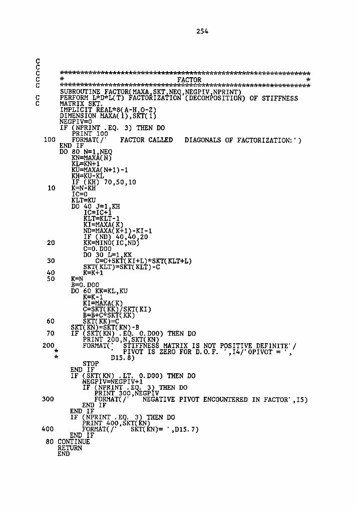
254
Sg
****2***«****«******«********«*****«***«****«*«**««*«***«««***C * FACTOR *c *«*«*«*«***«*«««*««***«2*******«*«***««*«*«*«*********««****«*SUBROUTINE FACTOR(MAXA SKT NE3,NEGPIV NPRINT&C PERFORM L*D*L(T) FACTORIZATIO (DECOMFOSITIO ) OF STIFFNESSC MATRIX SKT.IMPLICIT REAL*8(A-H 0-2)
IF 3) THEN DO100 ENDF0§MAT(/' FACTOR CALLED DIAGONALS OF FACTORIZATION:')
DO 80 N=l NEKN=MAxA(N?KL=KN+1
IF (KH) 70,50,1010 K=N-KH
IC=0KLT=KUDO 40 J=1 KHIC=IC+I
20 KK=MINO(IC:ND)gäoägog-1 KK
30 C=C+SKT(KI+L%*SKT(KLT+L)SKT(KLT)=SKT(KL )-C
40 K=K+150 K=N
B=0.DO0DO 60 KK=KL,KU
§I§MgXA(K)C=SKT KK /SKT(KIB=B+CiSKT(KK)
)
°° S¤N§§i5‘N§E€KN> B’° NN MN N°200 FORMAT(' °STIFFNESg MATRIX IS NOT POSITIVE DEFINITE'/
* ' PIVOT IS ZERO FOR D.0.F. ',I4/'OPIVOT = ',* D15.8)
EN¤N¥$"IF (SKT(KN§ .LT. 0.D00) THEN DO
NEGPIV= EGPIV+1IF (NPRINT .E3. 3) THEN DOPRINT 300, EGP V
300 ENDF0§MAT(/' NEGATIVE PIVOT ENCOUNTERED IN FACTOR',I5)
END IFNN ”°400 FORMAT(/', SKT(NN)= ',Dl5.7)
END IF80 CONTINUE
RETURNEND
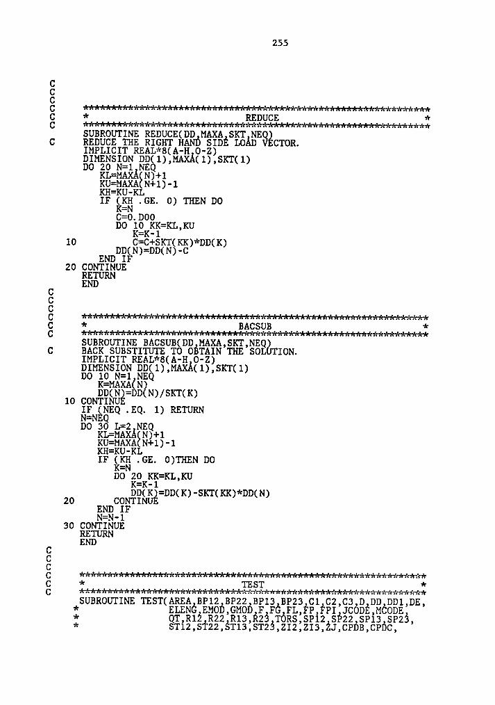
255
S8 ««*«****«*«******«****«*«****«*««*****«*««*«**««««««***««*****icE *«*****««****«*«******««*««««§§£gg£**«****«*«**«***«*****«*«*:SUBROUTINE REDUCE(DD MAXA SKT NESEc Rzoucz mz RIGHT HAND swf: LOÄD cTOR.
IMPLICIT REAL*8(A-H O-Z)DIMENSION DD(1),MAXÄ(1),SKT(1)CCIF
§Kg .GE. 0) THEN D0C=0.D00DO é0KKK=KL,KU
10 C=C+SKT(KK)*DD(K)DD(N)=DD(N)-C
END IF20 CONTINUE
RETURNEND
SC * BACSUB *CSUBROUTINE BACSUB(DD MAXA,SKT,NEQ&TC CCC CCC CCC
DIMENSION DD(1),MAXÄ(1),SKT(1)CC éC„§§äz§’§CDD(Ng=DD(N)/SKT(K)
10 CONTINUIF (NEQ .EQ. 1) RETURNN=NEQCC ä§;§§§ÄC§?+1
IF .GE. 0)THEN DODO §0KKK=KL,KU
DD(K =DD(K)-SKT(KK)*DD(N20 CONTINUE
)
END IFN=N-1
30 CONTINUERETURNEND
EE *****«**««*«******«*«******«*****««**««***********«*****«***«** *vh':¤'c·A·¤'¤'Hn'c*iv*ir1‘rv\·iric='c7\·1'rv\·1'v·!¢·ic='n'¢='d¢fH¢3Eg=§='£i:1'ci¢¤'¢ivi:=%=’ci:1'r=¥v%=':ik1':·A·=':v'¤'c=':v'c=':='r1’:=':=':¤':1':='r
SUBROUTINE TEST(AREA BP12 BP22 BP13 BP23 C1 C2,C3 D DD DD1,DE,
# STI2,ST22,$T13:ST23,ZI2:ZI3,ZJ,CPDB,CPDC,’
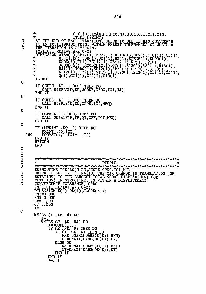
256
:CAT THE END OF EACH ITERATION CHECK TO SEE IF HAS CONVERGED
C TO AN EQUILIBRIUM POINT WITH1N PRESET TOLERANCES OR WHETHER
CDIMENSION AREA(1ß BP12(1) BP22(1 ,BP13(1g BP23S1) C1(1) C2(1),* C3(12 (12 ¤0(12 DD1 1 DE(1) LENG( EMOD(l),* 6M0¤ 1),F ig FG 12 1) L(12 lg FP(l) PI(l)« JCODE(6 lg ÖODE(12 1;,QT(1? 12(l) R22(1) Hl3(1),* R2s(1) To $(1) SP12(l spzz 1) SPl3$1g,SP23(1)* ST12(1%,ST22(1) ST13(12 ST23(1),ZI2 1 ,ZI3(1),ZJ(1),* Q(1),c l(l),CI2(1),CI3 1)
C ICI=OIF (CPDC .LT. l.D00) THEN DO
CALL DISPLC(D,DD,JCODE,CPDC,ICI,NJ)
C END IFIF (CPDB .LT. l.D00) THEN DO
CALL DISPLB(D,DD,CPDB,ICI,NEQ)
C END IFIF (CPF.LT. 1.DO0% THEN DO
CALL UNBALF(F, P,QT,CPF,ICI,NEQ)
C END IFIF (NPRINT .E¥. 3) THEN DO
PRINT 100) CI100 FORMAT(// ICI= ',IS)
END IFRETURNEND
SC * DISPLC *g
****«*********«**«**«*****««**«**«*«****«****«*****«**«*******SUBROUTINE DISPLC(D,DD JCODE CPDC ICI NJEC CHECK TO SEE IF THE RATIO: THE MAH CHÄNG IN TRANSLATION (ORC ROTATION TO THE LARGEST TOTAL NODAL DISPLACEMENT (ORC ROTATION IN STRUCTURE, IS WITHIN A DISPLACEMENTC CONVERGE CE TOLERANCE, CPDC.
IMPLICIT REAL*8(A-H O-Z)DIMENSION D(1),DD(1),JCODE(6,1)RMT=0.DOORMR=O.D0OCR=O.DOOCT=0.DOO
C I=1WHI§E1(I .LE. 6) DO
WHILE (J .LE. NJ) DO‘§§C€%2CC§é·C2„ THEN DOIF (1 Äcß. az THEN DORMR=DMAX1 DABS(D§K)g,RMR)ELSgR§gMAX1(DABS(DD K ,CR)RMT=DMAX1(DABS(D(Kgg,RMT)CT=DMAX1(DABS(DD K ,CT)
END IFEND IFJ=J+l
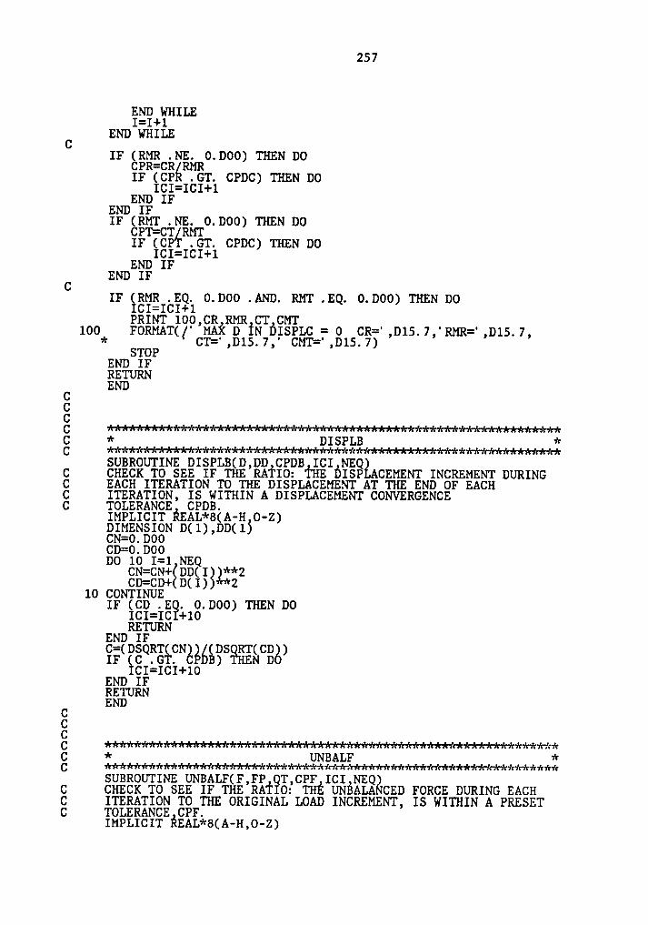
257
END WHILEI=I+1
C END WHILEIF (RMR .NE. O.D00) THEN DOCPR=CRéRMR
IF (CP .GT. CPDC) THEN DOICI=ICI+1
END IFEND IFIF (RMT .NE. 0.D00) THEN DOCPT=CT4RMT
IF (CP .GT. CPDC) THEN DOICI=ICI+1
END IF
C END IFIF (RMR .EQ. 0.DOO .AND. RMT .EQ. 0.D00) THEN DO
ICI=ICI+1PRINT 100,CR RMR CT CMT
100 FORMAT([' MAK D IN DISPLC = 0 CR=',D15.7,'RMR=°,D1S.7,* CT=‘,D15.7,' CMT=',Dl5.7)
STOPEND IFRETURNEND
C
8C *****************+*********+**************«******+**+********«C * DISPLB *C *****+******+**+**+*+*+*«*****+**w*+*****+*+******+«********+*SUBROUTINE DISPLB(D,DD CPDB ICI NEQEAC CHECK TO SEE IF THE RATIO: THE DISP CEMENT INCREMENT DURINGC EACH ITERATION TO THE DISPLACEMENT AT THE END OF EACHC ITERATION, IS WITHIN A DISPLACEMENT CONVERGENCEC TOLERANCE CPDB.
IMPLICIT REAL*8(A-H O-Z)DIMENSION D(1),DD(1$CN=0.D00CD=0.D00DO 10 I=1 NEQCN=CN+$DD(Igl:*2
CD=CD+ D(I) 210 CONTINUE
IF (CD .E?. O.D0O) THEN DOICI=IC +10RETURN
äN?DSäRT(CN (DS RT(CD )IF (C .GT. GBEB) ¥HEN DO
ICI=ICI+10END IFRETURNEND
C
SC *******+****+*+****w*+**«******+*******«*++******«*******«*«+*w +E **«*«***+*****«+******+*****g§£é£§***********«****+*«**+*«+***SUBROUTINE UNBALF(F,FP QT,CPF ICI NEQgC CHECK TO SEE IF THE RATIO: THE UNEALA CED FORCE DURING EACHC ITERATION TO THE ORIGINAL LOAD INCREMENT, IS WITHIN A PRESETC TOLERANCE CPF.
IMPLICIT REAL*8(A-H,O-Z)
258
DIMNSION F(1 FP(l T(lg§=g·B88 ), )„Q )00 10 I=l NE0CN=CN+€QTäIg-F(I}%**2
CD=CD+ QT I -FP( )**210 CONTINUEIF (CD .E?. 0.D00) THEN DORgI=IC +100
END IFC=(DSQRT(CN) (DS RT(CD)IF (C .GT. CR;) TEEN DO
)
ICI=ICI+100END IFRETURN
C ENDCg
*****+********w****+******«*****+*****«*****««***«******w++«**C *C ******«******«****«**«******«****+«+«*:SUBROUTINE RESULT(C1 C2,C3 D DJ ELENG EMOD GMOD FG,FL,* JCÖDE,MCÖDE Miwc P 0,0T ZI2,ZI3,« zJ,NE NEQ,NJ 01,iMP NPRINT)
E ħäTä3%%6¥ THE NODAL FORCE MATRIX ,P,T0 ZERO; CALL JOINTFIMPLICIT REAL*8(A-H 0-Z)DIMENSION C1(1 C2(1 C3(1 D 1 ,DJ(6 1 ELENG(1 EMOD(l
* GMODEI) FG212,1g?FL(12 12 Jé00éä6 lg MgÖDE(l2 15,* M1Nc 2,1),P(6,1 ,Q(l),ÖT 1),212 15, I3(l),ZJ(1)
DO 20 J=1 NJ00 10 I=l,6
10 001»¥&1£0ä"°·°°°20 CONTINUE
CALL JOINTF(FG MINC,P NEECALL OUTPUT D,DJ,FL,JCOD ,P,QT,NE,NEQ,NJ,QI,IMP,NPRINT)RETURN
C ENDC .gC
* JOINTF *C **«********««**+*************«********«*******«***««**********SUBROUTINE JOINTF(FG MINC P NEC ASSIGN THE GLOBAL ELEMENT’FÖRCES TO THE NODAL FORCE MATRIX,P.
IMPLICIT REAL*8(A-H,O—Z2DIMENSION FG(l2,1),MINC 2,l),P(6,1)DO 20 I=1 NE
1=¤1¤2$;·1200 10 L=i 6PäL,JgéP§L,J;+FGEL,I)P L K =P L,K +FG L+6,I)10 CONTINUE
20 CONTINUERETURN
C ENDCg
****************************kk%**ü********************%*%*k***C * OUTPUT *
259
C **************************************************#**kküüükäkkSUBROUTINE OUTPUT(D DJ FL JCODE P QT NE NEQ NJ,QI,IMP NPRINT)c PRINT THE N0¤AL DISPLACEMENTS (INCLUDINÖ NODAL CONSTRÄINTS)C DJ; PRINT THE LOCAL ELEMENT FORCES FL; PRINT THE NODAL FORCES,C P* PRINT THE LOAD VERSUS DISPLACEMENT VECTOR,QT AND D.
IMPLICIT REAL*8(A-H,O-2%DIMENSION D(1),DJ(6,l), L(12,1),JCODE(6,1),P(6,1),QT(1)DO 20 J=1 NJ00 10 i=1 6¤1(1 Jé=0.D00
K=1c00 (1,1)IF (K .NE. O? THEN DODJ(I,J)=D K)
END IF10 CONTINUE
C 20 CONTINUEIF (NPRINT .LE. 12 THEN DO
PRINT 100,QI D IMP)100 FORMAT(' ',F17.9/ ',F17.9)
C END IFIF (NPRINT .EQ. 2 .0R. NPRINT .EQ. 3) THEN DO
PRINT 200,QI,D(IMP)200 FORMAT(' QI EQUIL B =',F17.9,' D EQUILIB =',F17.9)
C END IFIF (NPRINT .EQ. 4) THEN DO
PRINT 300,QI300 FORMAT('- 80('_')§§31X,'QI=',F15.7//34X,'LOAD VECTOR'
* ysak 11('*00 30 1=1 NEQ
PRINT 400,QTäI)400 FORMAT('0 ,3 X,Fl6.5)
30 CONTINUEPRINT 500
500 FORMAT('-' 26X,'GLOBAL NODAL DISPLACEMENTS'/27X 26('*')* /41ÖX,' NODE' 7X,'1-DIRECTION' 8X,'2-DIRECTION'* 6 ,*9-¤1REcT10N* 8X,'4-DIRECTIÖN',8X,'S—DIRECTION',* 8X,'6-DIRECTION')
DO 40 J=1 NJPRINT 600,1 (DJ2I,J) I=1 6%
600 F0RMAT(· ,0X,I ,6(2X,F17. ))40 CONTINUE
PRINT 700700 FORMAT('-' 29X;‘LOCAL ELEMENT FORCES&630X,20('*‘)/
* ' ELE. 30X,'A—END',60X,'B-E '/' NUM.',3X,'1',* 9X,'2',9X '3 9X '4' 9X, 5' 9X,'6',9X,'7',9X,'8',9X,* *9 ,9X,'10',9X,'1l',9X, 12')
DO 50 J=1 NEPRINT 600,1 (FL(I J) I=1 12)
800 F0RMAT(*0 ,I2,l2(1X,F9.4))50 CONTINUE
PRINT 900900 FORMAT('-';33X 'NODAL FORCES'/34X 12('*')/10X ' NODE'
* 7X, 1-DIRECTION',8X,'2-DIRECTION',8X,'3-DIRECTION'* 8X,'4-DIRECTION',8X,'5-DIRECTION',8X,'6-DIRECTION')”°
31‘ä1§—?*6’ää 1 (111 11 1 1 61I I I I I60 CONTINUEPRINT 1000
1000 FORMAT('0',80('_'))END IFRETURN
C END
E 260
8C **********«*****«*******«*****«***«******«*«**««********«*«***C * DOTPRD *C ******«*««*******«************«***«**«***«********«*«**«*****«FUNCTION DOTPRD(DOT1 DOT2 NBC COMPUTE THE DOT PRODÜCT OP 0T1 AND DOT2.
IMPLICIT REAL*8(A-H O-Z)DIMENSION DOT1(1),DÖT2(1)DOTPRD=O.D00DO 10 I=1,N
DOTPRD=DOTPRD+DOT1(I)*DOT2(I)10 CONTINUE
RETURNEND
C
8C **«*«**********«««*****«**«***«***«**«******«**«***«**«*******C * UPDATE *C **««*******«**«*«**«****«******«*««**************«*****««*«***SUBROUTINE UPDATE(3T Q NEQ,QI)
mPL1c1T REAL*8(A· 6-Z)DIMENSION 3T(l),Q(15”° ‘·?« %=16«‘%‘§·«Q1
10 CON¥INUERETURNEND
CC//DATA