' Globalization' and Vertical Structure

byJohn McLaren, Columbia University

July 1996

Discussion Paper Series No. 9596-24

'Globalization' and Vertical Structure.

John McLarenDepartment of Economics

Columbia UniversityNew York, New York 10027

jeml8@columbia.edu

July, 1996

I am grateful for extremely helpful comments to Patrick Bolton, Jay Choi, Faruk Gul, ChrisSanchirico, and especially Andrew Newman. Many helpful suggestions were offered byseminar participants at the NBER Summer Institute International Trade and Investment group,July 1996. All remaining errors are my own.

Abstract.

This paper analyzes the effects of international openness on verticalintegration decisions. A simple model is presented to represent theasset specificity problem at the heart of many industrialorganization economists' analysis of vertical integration. Itsuggests that there is a kind of negative externality conferred byeach vertical integration, by 'thinning' the market for inputs andthus worsening opportunism problems; thus, in equilibrium theretends to be too much of it. Further, vertical integration features akind of strategic complementarity, which can lead to multipleequilibria in the outsourcing decision, thus providing a theory ofdifferent 'industrial systems' or 'industrial cultures' in ex anteidentical countries. In addition, the country that gets stuck in ahighly vertically integrated equilibrium suffers from lowerefficiency. Greater international openness forces convergence inthe degree of outsourcing across countries, and facilitates leaner,less integrated firms, thus providing a channel for welfareimprovements from international openness that appears to be quitedifferent from those that are familiar from the trade theoryliterature. This may be taken as one theory of 'outsourcing,''downsizing' and 'Japanization' as consequences of 'globalization.'

Much of topical economics implicitly or explicitly concerns changes in vertical integration

decisions of industrial corporations. For example, the phenomenon of 'downsizing' often has a

strong element of vertical divestiture1. Strong trends in 'outsourcing2' have been observed in

recent years in many industrial sectors3. The differences in industrial 'systems' across countries,

for example, between the U.S. and Japanese economies, have much to do with differences in

vertical structure, with Japanese industry very much less integrated than its major trading

partners4.

All of these trends in vertical structure are at times claimed by various observers to have

a strong relationship with international trade. Downsizing is held to be a response to increased

foreign competition; the leaner organizational structure of Japanese industry allegedly gives it

some advantages which have forced a partial 'Japanization' of some Western industries5.

However, the logic in each case is far from clear, and there does not appear to be a body of

'This was driven home emphatically by the brake workers' strike that crippled GeneralMotors this past spring; the principal issue was GM's desire to outsource more of its brakeproduction.

throughout this paper, the term 'outsourcing' will mean the provision of an input outsideof the firm that will use it, not necessarily outside of the country in which it will be used.This appears to be a difference in usage between the industrial organization and trade theoryliteratures.

3See Gardner (1991) for the rise in outsourcing of data management by hospitals; BankSystems & Technology (1991) on outsourcing of technology by banks; Buxbaum (1994) onthe recent outsourcing of distribution services by GM; Bamford (1994) on the recent trendtoward outsourcing of parts in the U.S. automotive sector; Bardi and Tracey (1991) on themove toward greater outsourcing of transport services across manufacturing; and Economist(1991) for an overview of the trend toward outsourcing in manufacturing in general.

4See Nishiguchi (1994) for an extensive analysis of the Japanese case; Morris (1991) andGertler (1991) offer comparisons with North American industry. See also Economist (1991).Similar comments are sometimes made about small-firm industrialization in the 'Third Italy'of Emilia-Romagna and other regions; see Gertler (1991, pp. 380-5) for a review.

5See, for example, Gertler (1991).

2

theory within international economics to address these questions. Can a rise in openness affect

the vertical structure of industry in a predictable way? If a 'leaner' organizational structure really

is a lower cost way of procuring inputs6, why would, say, an American auto firm wait until it is

battered by competitors to implement it? Why would a profit-maximizing corporation not always

choose to minimize costs? Further, does any of this have welfare implications?

This paper analyzes the effects of international openness on the vertical integration

decision in an industry equilibrium, and suggests that openness can indeed have strong effects

on vertical structure, and that this can have large welfare effects. A simple model is presented

to represent the asset specificity problem at the heart of many industrial organization economists'

analysis of vertical integration. It suggests that there is a kind of negative externality conferred

by each vertical integration, by thinning the independent market; thus, in equilibrium there tends

to be too much of it. This can lead to multiple equilibria in the outsourcing decision, thus

providing a theory of different 'industrial systems' or 'industrial cultures' in ex ante identical

countries despite profit maximizing behaviour. Nonetheless, globalization forces convergence in

the degree of outsourcing across countries, and there is a presumption that it results in less

vertical integration, thus providing a role for welfare improvements for international openness that

appears to be quite different from those that are familiar from the trade theory literature.

The outlines of the argument are as follows. In this model, each of a number of final

goods producers ('downstream firms,' or DSF's) tries to procure a specialized, indivisible input

from a supplier (or 'upstream firm,' or USF). Each USF can produce one unit of specialized

6As argued forcefully by, among many others, Nishiguchi (1994) and Economist (1991).See also the recent consultant's report on the US auto industry cited in Maynard (1996),which pushed outsourcing very hard.

3

input. There are two possible procurement methods: 'arm's length,' or market, procurement; and

'integrated' procurement. In the former, the two firms form an understanding, perhaps through

a verbal agreement, and come to terms on payment when the unit is ready. In the latter, some

costly commitment technology is brought to bear, either a long-term contract or a merger between

the two enterprises. This dichotomy is, of course, meant to capture some of the key issues in

choosing the degree of vertical integration; in practice there is a continuum of such degrees

available.

Because of the sunkeness of the cost of producing the input and its specialized nature, the

USF knows that under the arm's length arrangement it is in danger of being 'held up' by the DSF

and not recouping its costs ex post. Its only reassurance is that there may be alternative uses for

the input beyond the DSF for which it is intended, which will give the USF bargaining power

and allow it to demand a remunerative price. Thus, in the absence of a robust potential market

for the input, the USF may judge the input to be an unremunerative product and abandon it. The

alternative is the integrative arrangement, but this has its own disadvantages; either legal costs

from negotiating and enforcing a contract or the costs of a merger and its attendant heightened

'governance costs.'

Thus, as argued in an extensive literature, each DSF/USF pair in the industry chooses

between the two methods by trading off the 'hold-up' problem of arm's length trade against the

'governance costs' of the integrated solution7. However, three consequences of this reasoning

are noted which are not much acknowledged in the existing literature. First, the feasibility of the

arm's length system depends on the USF's prospects for recovering its sunk costs on the open

7This language is most closely associated with Willamson (1971, 1989).

4

market; but these prospects are better the more of the other firms have chosen arm's length

arrangements (or, the 'thicker' is the secondary market). The reason is that the equilibrium price

received by an unintegrated supplier is determined by the input's most attractive alternative use,

and the expected value of this is higher, the more alternative uses there are8. Since an

unintegrated DSF is much more likely than an integrated one to be a potential alternative use for

inputs from independent suppliers, it is thus natural that a rise in the number of unintegrated

firms makes unintegrated supply more remunerative. This is Proposition 6 of the paper. There

is thus a negative externality from vertical integration, making arm's length arrangements less

feasible for others. For this same reason there is a 'strategic complementarity' in the vertical

integration decision9, so if the firms in the industry are sufficiently similar, there can be two

equilibria: one with each firm choosing integration, and the other with all input suppliers

remaining independent. One interpretation of this is that two otherwise identical countries can

have completely different 'industrial cultures' or 'industrial systems' without in any way

departing from strict assumptions of economic rationality or profit mazimization.

Second, an additional means of thickening the secondary market is to open up the

economy to international trade. If two countries have similar industries facing the 'hold-up'

problems described above, then lowering trade costs between them will make it easier for an

input supplier to find an attractive alternative buyer abroad, thus strengthening its bargaining

8Put differently, an input's price is determined by the second order-statistic of a finitesample; raising the sample size clearly raises its expected value.

9This sort of effect might also be present in the seminal analysis of Hart and Moore(1990) if only there was not an efficient industry-wide ownership contract worked out at timezero. In the present paper, ownership arrangements are worked out only bilaterally.

5

power ex post and making an arm's length arrangement more attractive. Thus, international trade

can in principle lead to a substantial increase in the incidence of arm's length trade. Further,

procurement systems across countries will tend to 'converge' with increased openness. There is,

in addition, a sense in which increases in arm's length trade tend to be 'internationally

contagious'.

Third, since a thickening of the market simply gives each firm more options in its

procurement strategy, the effects of the opening up of trade on vertical structure are

unambiguously efficiency enhancing. They thus provide an avenue for efficiency benefits of

open trade that are completely separate from the well-understood avenues of increased

specialization and competition, and which seem to be completely unacknowledged in the trade

theory literature.

This paper builds on a well-established tradition in industrial organization which has not

been put to much use in trade theory. The 'transactions cost' approach to vertical integration has

been espoused by Williamson (1971, 1989) and Klein, Crawford and Alchian (1978). Although

it is by no means the only important theory of vertical integration (see Perry (1989) for a survey),

it has been shown to have a certain empirical explanatory power, as for example in Joskow

(1987), Monteverde and Teece (1982), and Masten (1984), each of whom shows that in the data

examined a greater level of 'integration' is predicted by a greater degree of asset specificity10.

The incentive effects of different ownership structures in the context of specific investments and

10In the former study, which examines relationships between electric utilities and coalsuppliers, the degree of integration is measured by the length of contract between the twofirms. The second study looks at the make/buy decision among U.S. automobile producers,and the third in the aerospace industry.

6

incomplete contracts are studied in Grossman and Hart (1986), Hart and Moore (1990), and

Bolton and Whinston (1993). Vertical integration emerges in some cases as the best response

to the incentive problem. In the international trade literature, Spencer and Jones (1991, 1992)

study the effects of vertical integration on strategic trade policy, without endogenizing the vertical

integration decision.

Despite the richness of the literature on which it draws, the model used here has a number

of novel features. It combines a simple formulation of the idea of technological serendipity with

the finiteness of the set of firms in a given sector to provide a meaningful sense of the 'thickness'

of a market11. It allows for endogenous choice of the degree of asset specificity by input

providers, a decision which is affected by the integration decision and which in turn has its own

effect on secondary market 'thickness.' In combining these elements, the model further shows

how vertical integration by one pair of firms can confer a negative externality on the rest of the

sector, thus pointing out that the analysis of the bargaining problem carried out by a number of

pairs of firms in an industry can be qualitatively different from the analysis of a single pair of

firms in isolation12. Although the model is itself quite special, these features in some form are

likely to survive a number of kinds of generalization; this is discussed at the end.

Section 2 sets up the model; section 3 studies the determination of prices on the

nThis concept of 'thickness' has a close relationship to the concept used by Telser (1981)to identify the advantages of organized futures markets.

12Another paper that focusses on horizontal interactions between firms in verticalintegration decisions is Bolton and Whinston (1993). That model is built with two DSF's andone USF, and a random capacity for the USF so that the issue of 'supply assurance' plays akey role. A different kind of negative externality from vertical integration emerges in thatcase: The expected profit of the DSF left out of the arrangement falls, because it makes theintegrated firm very aggressive in non-contractible investment.

7

independent market; section 4 derives equilibrium in the case of symmetric firms ('utter

homogeneity'), which tends to give corner solutions; section 5 studies the case in which the firms

are different enough that interior solutions are possible (the case of 'wide diversity'). Section

6 considers some alternative approaches.

2. The Model.

First we sketch the closed-economy version of the model; the open-economy version will

then be straightforward. Consider an economy with an 'industrial' sector composed of n firms

producing differentiated products, and an 'agricultural' sector, producing a homogeneous good

under perfect competition. Suppose that all consumers have utility function13 of the form

V(x]? x2,..., xn) + y, where x, denotes consumption of the ith 'industrial' good and y denotes

consumption of the 'agricultural' good. The latter is the numeraire, and is produced with

Ricardian technology with a marginal product of labor equal to unity, so that the wage is always

unity as well. Each industrial good is produced with a fixed labor requirement and a constant

marginal labor requirement; entry into that sector is prohibitively costly. Bertrand pricing

determines the price and gross profit of each of the n firms; because of the separability of

demand, these profits will be unaffected by any change in aggregate wealth.

Each firm in the industrial sector can reduce its fixed costs to some degree by procuring

13We will assume that the agents in the model maximize expected utility in cases inwhich there is a decision to be made under uncertainty. Given that, the form of the utilityfunction implies risk neutrality with respect to income.

a specialized input14. These inputs can be tailor-made for the firm by entrepreneurs, who require

K>0 units of labor to design and produce one unit of specialized input. This process takes two

periods: The cost is incurred, irreversibly, in period 1, and the output is obtained in period 2.

Call the input maker an upstream firm ('USF') and the firm interested in purchasing the input

a 'downstream firm' ('DSF'). Each DSF can make use of at most one unit of specialized input,

and each USF can produce only one unit.

Because of the lag between the costs and the output, the USF needs some

reassurance that it will be paid remuneratively. To focus on the choice of organization forms,

we assume that third-party verification problems preclude the possibility of purely contractual

solutions15; see the discussion below. This leaves two possible solutions. The first is the

'integrated solution,' in which the two partners form a merger; this would involve internal

'governance' costs, denoted L. We will denote the integrated firm resulting from the merger of

USF, and DSF, as IF,. Under the second solution, the USF simply produces the unit and

anticipates bringing it to open the market, hoping to fetch a high enough price ex post to recoup

its costs. This we will call the 'unintegrated' or 'arm's length' solution16, the use of an

14It would be natural to allow such inputs to affect marginal costs as well, but theresulting price effects would be a tremendous source of additional complication, and are notnecessary to get to the main points of the paper. Further, it would open up the possibility ofvertical integration for the purpose of 'vertical foreclosure', a motive very different from thetransactions cost motive that is the focus here. This is the subject of Hart and Tirole (1990),Ordover, et. al. (1990), and, in the international context, Spencer and Jones (1991).

15This is simply to keep the options for each firm pair down to two. A similar analysiscould be performed with contracts as an additional option, provided that there were limitationsor costs associated with them so that contractual solutions were not always optimal.

16The term is being used quite narrowly here. For a much richer conception of whatarm's length relationships mean, see Cremer (1996).

9

'independent supplier,' or simply the 'market' solution.

'Governance' costs, or more broadly, managerial incentive costs of integration, are widely

discussed in the economics literature17. We will have nothing new whatsoever to say about them

here. For a particularly simple and extreme way of making them concrete, suppose that

production of an input requires a U-asset and U-manager; production of the final good sold to

consumers requires a D-asset and a D-manager. There are actions a U-manager needs to take

from time to time to ensure that the asset will be useful, and there are actions a D-manager needs

to take from time to time to ensure that the downstream operation will be profitable. Call these

actions 'managerial care'. Suppose that the quality of the input is not verifiable to a third party,

hence not contractible; thus, it is not feasible to write a contract conditioned on the delivery of

a useful input18. Suppose that 'managerial care' is unobservable to anyone but the manager, and

hence not contractible; further, it involves some effort and consequently some disutility to the

manager. Thus, these actions will not be performed unless the manager owns the asset, and so

each asset must be managed by its owner19. In the case of a merger, this implies that the same

manager is managing two assets. We assume that there are diminishing returns to managerial

attention, so that this causes an increase in fixed costs equal to L>0 if one asset is a U-asset and

the other is a D-asset, and M>0 if they are both D-assets. We further assume that M is large

17See Williamson (1971, 1989) for extensive treatments; Calvo and Wellisz (1978) for aformal model; Grossman and Hart (1986) and Hart and Moore (1990) for treatments includingthis sort of incentive effect as part of a more general class.

18This precludes a simple contractual solution such as Noldeke and Schmidt (1995).Complicated contractual revelation mechanisms such as in Rogerson (1992) may still bepossible, but for our purposes we will suppose that they are impractical.

19Obviously, more generally the manager could own some fraction of the equity. Thebasic point is the same.

10

enough that horizontal integration is never profitable, simply so that we may focus on the issue

of vertical integration.

In an initial period of bargaining, each DSF simultaneously arranges with a USF which

of these two solutions will be pursued. Under the integrated solution, the two bargain ex ante

and strike a deal, splitting the surplus net of contract costs L; the merged entity then designs and

produces the input using the expected-profit-maximizing choice of technology. Under the arms'

length solution, the two partners may meet and form a mutual understanding ex ante, perhaps

through a verbal agreement, but there is no commitment on either side. The USF decides

whether or not to advance; if it advances, it incurs the fixed cost K in period 1 and chooses the

technology strategy to follow; in period 2 it receives the output and announces that it is accepting

bids on it. The input is then sold to the high bidder, ending the game. The sequence is

illustrated in Figure 1.

The USF is assumed to have

Initialdiscussionon integration.

Sunk cost isincurred;Specializationdecision is made.

Input arrives;benefit matrix,R, is revealed.

Bids areplacedfor inputs.

Figure 1. The Sequence of Events.

two options in its design strategy: a

s t r a t e g y of ' m a x i m a l

specialization'and a strategy of

'flexibility.' In the maximal

specialization strategy, the input is

designed in such close accordance

with the peculiarities of the production process of the DSF in question that it would be useless

for any other purpose. Define the cost reduction offered by the input designed for DSF i, when

used by DSF j , as R . We will refer to the matrix R as the 'benefit matrix.' Then under a

Exchangeoccurs.

11

strategy of maximal specialization, K1} = 0 if i^j. We normalize R,, in this case to unity. On the

other hand, the design process could allow more room for the input to be compatible with other

systems; since those other systems are likely to be less familiar to the USF, its uses with those

systems are more likely to have a serendipitous nature20 than the gains from the specialized

technology strategy. These specialization decisions could be interpreted, for example, as

choosing the degree of 'site specificity'21 or 'design specificity'22, to use Williamsonian terms.

This is incorporated into the model as follows.

20This implies a sort of uncertainty that can be extremely important in practice, especiallyin new or rapidly developing technologies. In a rapidly changing technological environment,the relative merits of alternative designs typically can not be identified at the design stage.Examples of ex ante uncertainty of this sort are legion; see Vincenti (1994) for an account ofuncertainty in the 1930's about whether retractable landing gear or various alternatives wouldprove superior, and Numagami (1996) for an account of similar uncertainty in the 1970'sabout which design for digital watches would prevail.

21This is specificity resulting from physical proximity. For example, a coal-burningelectric utility may become very specialized to a particular mine by locating close to the minemouth; utilities have a wide variety of choice in such location decisions (Joskow, 1987). Inthe aerospace industry, there are large cost savings to be had by locating the computerizedlathe for boring nose cones near the assembly plant in which the cones will be used; but oncethe lathe has been installed, it is extremely costly to move it. Thus, the location of the latheis an important determinant of its specialization toward a particular assembler (Masten, 1984).

22This is specificity resulting from the design process per se. For example, a softwaredesigner may write a program to fit the peculiarities of a single firm's business, or maydesign it for the mass market as packaged software; the vast majority of the output ofJapanese software houses fits the former category, and is never sold on an open market, insharp contrast to the American system (Baba, et. al, 1995). For another example, MeltonTruck lines provides customized shipping services for Butler Manufacturing, which assemblespre-fab buildings for Wal-Mart in Mexico. The shipping jobs are complex and involve muchcoordination of different components and of border paperwork. Melton had a computerizedsystem for this purpose, but it went the extra step of redesigning its own informationmanagement system to integrate it with Butler's system and provide a more effective service(Buxbaum, 1996). A notorious example of endogenously chosen asset specificity is the caseof IBM in the 1970's redesigning its mainframe computer interfaces to make it difficult fornon-IBM hard drives to be used with them (Brock, 1989).

12

Let the probability density function for R14 under the flexible technology strategy be given

by h:[0, 1]-»R, with jx h(x)dx > K. Let g:[0, l]x[0, 1]-»R be a non-negative valued function

satisfying:

(i) j ; g(y; x)dy M V x e [0, 1];

(ii) g(y; x) > 0 for x, y e [0, 1] with y<x;

(iii) g(y; x) = 0 otherwise.

Thus, g is the probability density function, conditional on a variable x, for a random variable y

on [0, 1] whose value never exceeds x. Now, if a USF has designed an input for DSF i, and has

used the flexible technology strategy, we can speak of the ex post 'suitability' of the input for

use with DSF j as measured by a random variable xtJ e [0, 1], where a value of 1 means complete

suitability and a value of zero means complete unsuitability, and where xt = (xn, xl2, ..., xm) has

a density function \y given by:

\j/(x,) = h(xu) n^gCxiji xn).

Thus, the input is always most suitable for its intended use, but it may happen to have other uses

that are almost as suitable. These suitabilities are realized as soon as the input is produced, and

at that moment they become known to all.

This input then can offer potential cost reductions to the various DSF's as follows:

13

if i*j

where ( e [0, 1] is an exogenous constant. Thus, the greatest possible cost reduction is to its

intended DSF; this cost reduction is less than would it would have been under maximal

specialization23; but if ( is not too small, the potential cost reductions for other DSF's might still

be substantial. The parameter ((), can be called USF i's "scope for flexibility." If it is close to

zero, there is not much the USF can do to allow for alternative uses for its product. It will be

a convenient parameter to vary in what follows.

An important consequence of these assumptions (particularly (iii) above) is that for either

technology strategy:

(1) RJJ > Ry with probability 1 for all i, where j^i .

In short, under an arm's length arrangement, a USF designs an input, choosing specialized

or flexible technology; once it is ready, the USF brings it to the market and sells it; after that,

the game ends.

In the case of the open economy, there will be two countries which will be identical in

every way. There will thus be 2n firms; those numbered 1 through n will be in country I and

the following n will be in country II. The density function given above for the 'suitabilities' of

23It would not change anything of interest to allow Rh under maximal specialization to berandom as well, provided that it was greater in expectation than Ru under flexibility.

14

the n firms in one country will extend in the same way to the 'suitabilities' for the other

country's firms as well. In order to focus on the vertical structure aspects of the situation and

to make the point that the effects of openness in this model have nothing to do with well-

understood effects through product-market competition, assume that the n final goods produced

in each country are unattractive to consumers in the other, so that the final goods are effectively

nontraded. Inputs, on the other hand, can be traded across the border at a cost of t. Thus, if i<n

and j>n, for an input i, RtJ = {^x-t} if it is designed with flexible technology, and R = -t if it

is maximally specialized. Apart from these changes, the open-economy version of the model

works in the same way as the closed-economy version.

3. Ex post price determination.

To solve the model, we work backward from the determination of prices and input

allocations on the open market. For the moment assume a closed economy.

Once the n inputs have been produced, the matrix of R values is known, and the various

DSF's can send bids (simultaneously) to the various input makers. Let bX] denote the bid made

by buyer i for input j (for the moment allowing for the possibility that either firm i or firm j is

integrated24; an integrated firm always have the option of selling its input or of placing a bid for

another firm's input). The bids are made simultaneously and each represents a commitment to

buy the stated input at the stated price, provided the seller accepts the bid. It will be convenient

to define the vector of winning bids P by P, = max^b^}, which can also be called the vector of

24But not both; it would be meaningless for an integrated firm to bid for its own input.

15

equilibrium prices. Without loss of generality we restrict bids to be non-negative. In addition,

since there is no meaningful difference between a bid of zero and no bid, we will without loss

of generality require each potential buyer to place a bid of at least zero each input (except for

an integrated firm's own good). Note that there is no contradiction between the impracticality

of an ex ante contract to buy and the desirability of an ex post commitment to buy. Since quality

is not contractible, an ex ante purchase contract would guarantee receipt of a worthless asset, by

removing the incentive of the U-manager to take proper managerial care, as discussed above.

However, once the input has been produced, that is not an issue.

Ignoring for parsimony costs incurred at earlier stages of the game, the payoff to an

unintegrated DSFj is given by the maximum of RJt for jeS(i), minus S^^by, where S(i) is the

set of bids made by i that were accepted by the respective sellers. (Recall that i can make use

of at most one unit of the input.) The payoff to an unintegrated USFj is equal to max^by}; the

USF simply accepts the high bid, perhaps randomizing over ties. The payoff to an integrated

firm IFj is the maximum of: max (R,,, max^^R^}) minus XjgsQ ij (which it receives if IFX does

not accept a bid for its own asset); and maxjeS(l){Rjl}+maxk{bki} minus Xjgs by (which it receives

if it does).

To eliminate some technical nuisances, assume that the bids must be made in discrete

units of currency; thus, for some 8>0, all bids must be an integer multiple of £. The symbol [x]~

will denote max{y| y is an integer multiple of £, and y<x}. We will be interested only in what

happens as e becomes small. It is very important to keep in mind that the difference between

Pb the winning bid for any good, and the second-highest bid for that good, can never exceed e

in a Nash equilibrium.

16

We will be interested in Nash equilibria of this bidding game, in order to discuss subgame

perfect equilibria of the full game. Propositions 1 through 5 provide a characterization. The first

point to note about these Nash equilibria is that their outcome is ex post efficient.

Proposition 1. In any Nash equilibrium of the bidding game, with probability 1, if e is small

enough, no IF sells its input, and each independently produced input is sold to its originally

intended buyer.

Proof. Suppose that in some equilibrium this is not so. In that case, denote z(i) as the input

finally used by buyer i. In no Nash equilibrium will any buyer buy more than one input, or any

input go unused, so the function z is invertible. Set M = {i | z(i)^i}? and note that z(M) = M.

If jeM, then buyer j chooses to purchase input z(j) rather than j ; if j is unintegrated, she could

have purchased j for P3+e, so we must have:

R J J " P J " £ ~ Rz(j)rPZG)-

If j eM is integrated, she has sold input j for a price of P, instead of using it herself, so:

Kfi * RZ0)rPz0)

+Pr o r

RJJ~PJ - RzG)j~Pz(j)-

Thus, if we denote by n the number of independent firms in M, we must have:

Since M = z(M), this implies:

17

^jeML^-iiJ"ne — 2ijeM[Rz0)jJ = ^jsML-^-j z(j)L

where the last equality follows from the invertibility of z. From (1), as e becomes small this

must become false. QED.

This considerably simplifies the problem. It allows us to write the condition for a Nash

equilibrium as the condition that for each i and j , buyer j prefers to buy the input designed for

her at price Pj rather than outbid buyer i for input i:

R^-Pj > Rij-Pi-e for all i25,

which implies:

(2) Pi > max] {maxOVRa+Pj, 0)}-e.

Since it shows that integrated firms will not engage in any purchase or sale in the market

stage, Proposition 1 also implies an immediate corollary:

Proposition 2. In a subgame perfect equilibrium, any integrated firm will choose the maximally

specialized technology.

25If j is integrated, this condition is unchanged. The payoff from keeping input j is R ;the payoff from selling it and buying another is PJ-(P1+e)+Rlj. The latter must not exceed theformer, and this is the stated inequality.

18

Any other choice would reduce EfRJ without having any other effect on IF,'s profits.

We obtain a further characteristic of equilibrium by eliminating weakly dominated strategies from

the strategy set, thus leaving only 'perfect' equilibria. In the context of this bidding game, this

set of strategies includes any bid by any buyer i for any input j such that bij>Rji, since lowering

such a bid to [RJ2]" will either raise i's profit or have no effect. Focussing on equilibria satisfying

this refinement immediately tells us that if good i is maximally specialized, b^O for j^ i , since

then Ry= 0 for j*i . Thus:

Proposition 3. As £->0, the equilibrium price of any maximally specialized good in a perfect

equilibrium goes to zero. In particular, in any perfect equilibrium of the full game, the

equilibrium price of any input produced by an integrated firm goes to zero.

It is therefore obvious that an unintegrated supplier would never choose the maximally

specialized technology. As a consequence of Propositions 2 and 3, we see that an input is

produced with flexible technology if and only if it is produced by an unintegrated supplier. There

is an exact correspondence between ownership structure and technology choice.

These conditions narrow the outcomes quite a bit; however, there are in general multiple

equilibria of the bidding game even after eliminating weakly dominated strategies. As an

illustration, consider the case in which n = 2, no firm is integrated, input 1 would offer 10 units

of cost reduction to DSFj and 9 to DSF2, and input 2 would offer 5 units of cost reduction to

DSFj but 7 to DSF2. Suppose that all integers are divisible by £. The bidding game here has

a range of perfect equilibria. One example is: [bn, b12, b21, b22] = [9, 5-e, 9-e, 5]; each DSF bids

19

for the other's designated input just e below the gross cost reduction that input would give her,

and for her own designated input the minimum bid required to acquire it, £ plus the competing

bid26. We might call this the 'high-price' equilibrium. By contrast, [2+e, 0, 2, e] is also an

equilibrium for the same benefit matrix. We might call this the 'low-price' equilibrium. We

need to make some sort of equilibrium selection, since the difference in payoffs between these

two is enormous.

Here the selection will be based on the following odd feature of the high-price

equilibrium. Consider DSFj's profit on its successful bid for input 1, valued at 1, compared with

its profit should its losing bid for input 2 be accepted instead. That hypothetical profit would be

(5 - [5-eJ) = e. Clearly, it would strictly prefer to lose its bid for good 2. Similarly, DSF2 earns

(7 -5) = 2 on its winning bid for input 2, but would earn £ on its bid for input 1 if that were

accepted instead, and so DSF2 strictly prefers to lose its bid for good 1. The natural question is:

Why, then, would it place that bid? Of course, in equilibrium it does not matter, since it does

lose the bid after all, but it seems to be a weak reed to support a high-price equilibrium solely

with losing bids placed by firms that would have no interest in winning them. By contrast, in

the low-price equilibrium, DSF2 makes a profit of (7-£) on its winning bid, and would make a

profit of 7 on its losing bid for input 1 if that were accepted instead; DSFj strictly prefers to win

its own input and does not bid anything for the other input. We will restrict attention to

equilibria in which the only non-zero losing bids a firm ever places are bids that would be at

26It is easy to check that this is a Nash equilibrium. DSFj buys input 1 at a price of 9,receiving a profit of (10-9) = 1; the best alternative move would be to buy input 2 instead, forwhich the lowest price would be 5+£. This would give a profit of -£, so the deviation wouldbe unprofitable. Analogous reasoning for DSF2 shows that its bid is optimal given DSFj's.

20

least as profitable as its winning bid, in the odd event that that bid were accepted instead. This

is summarized by requiring that for any buyer j and input i, either:

or bji = 0. We might call this the "only desirable bids" (ODB) condition. It can be written this

way:

bji < max (Ry-R.+b^, 0) = max (R1J-RJJ+PJ, 0),

so that

(3) ^ = bH < max^bjiJ+e < maXj {max (R^

Putting this together with the Nash equilibrium condition (2) tells us that in the limit as £—>0,

any ODB equilibrium price vector P can be written as27:

(4) P = TR(P),

where for any benefit matrix R, TR() is an operator on R£ such that for any n-vector q, the i01

component of TR(q) is:

[TR(q)L = maXj {max (R1J-RJJ+qJ, 0)}.

27From this point on, we will look only at the limit as e—>0, so this qualification should beunderstood in the statement of all subsequent propositions.

21

Equation (4) has a simple intuitive meaning. The term R -Ry+Pj can be read as the most

that buyer j would be willing to pay for input i, given that the price of input j is P r If R^Ry,

input i would do a better job for buyer j than j ' s own custom-made input, and j would be willing

to bid more for it as a result.

Note that there is no contradiction between the fact that R > R whenever i^j and the

possibility that Ry might exceed Rjr The distinction between the two is much like the difference

between absolute and comparative advantage. The statement that Ru > R for all firms implies

that the most efficient allocation of inputs is to place each one in the DSF for which it was

designed, and is much like saying that each input's comparative advantage is with its intended

use. However, the statement that Ry > R means that disregarding its opportunity cost, input i

would produce a larger benefit to DSF3 than the input designed for DSFJ5 and is much like saying

that input i has an absolute advantage over input j in serving DSFr This is what might give USF1

a possibility to enjoy a remunerative price: the higher its input's absolute advantage in use j , the

more buyer j will be eager to bid for it, even in the low-price equilibrium. Figure 2 illustrates

a case in which each of three firms' tailor-made inputs has a comparative advantage in use for

that firm, but input 3 has an absolute

advantage in all of them. This distinction is

key to the logic of the model: The workings

of the bidding game can be summarized by

suggesting that comparative advantage

determines the allocation of inputs, but

absolute advantage determines the distribution

R33

R>i.

R32

Rn=R22

R2.=Rl3 •

Ri^Riz

X

Cost reductionfrom input 3.

Cost reductionfrom input 1.

Cost reductionfrom input 2.

1Use to which D S F i D S F i D S F ]

input is put:

Figure 2. A Sample Pattern of Cost Reductions.

22

of income.

Equation (4) further tells us that in any ODB equilibrium, the price of any good, if it is

not zero, is determined by a 'chain of absolute advantage.' More precisely, for an equilibrium

price vector P and for any i, define A,(i; P) = argmax^, {R-R^+Pj} if this maximum is non-

negative28, and set X(i; P) = i otherwise. We can say that X(i; P) then identifies the 'runner-up

bidder' for input i in equilibrium, with A,(i; P) = i if and only if Pt = 0. We then have:

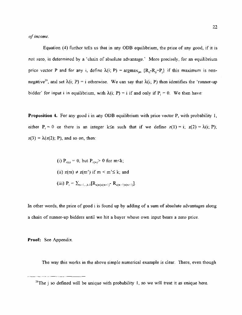
Proposition 4. For any good i in any ODB equilibrium with price vector P, with probability 1,

either P, = 0 or there is an integer k<n such that if we define z(l) = i; z(2) = X(i; P);

z(3) = X,(z(2); P), and so on, then:

(i) Pz(k) = 0, but Pz(m)> 0 for m<k;

(ii) z(m) ^ z(m') if m < m'< k; and

( i l l ) P j — 2 i m = i;..jk-lL

In other words, the price of good i is found up by adding of a sum of absolute advantages along

a chain of runner-up bidders until we hit a buyer whose own input bears a zero price.

Proof: See Appendix.

The way this works in the above simple numerical example is clear. There, even though

28The j so defined will be unique with probability 1, so we will treat it as unique here.

23

DSF2 can obtain its own designated input virtually for free, it still is interested in bidding for

input 1, since that input offers an absolute advantage of (9-7) = 2 in use by DSF2. Thus, DSF2

bids 2 for that other input. This is what forces DSFj to bid slightly above 2 for input 1. At the

same time, since good 2 offers no absolute advantage to DSF1? DSFj bids nothing for it. This

is what allows DSF2 to get it for free.

Finally, it is not difficult to show that the equilibrium can be simply calculated:

Proposition 5. There is a unique ODB equilibrium, and it is given by P = [TR]nl(0), where 0

is a vector of n zeroes, and [TR]nl denotes application of the TR operator n-1 times in succession.

Proof: See Appendix.

The ODB equilibrium has attractive properties aside from those mentioned above29, but

for the sake of robustness the consequences of making a different equilibrium selection will be

discussed in section 6.

Now we can discuss the equilibria of the full model. We do this under two contrasting

assumptions about the way the scope for flexibility differs across firms; first, the assumption that

it does not vary at all (the case of 'utter homogeneity'), and then the assumption that it varies

29For example, it can be shown using results from Giil and Stacchetti (1996) that it isequal to the marginal social value vector for the various inputs, in the sense that if P is theODB price vector, and if an additional copy of input i was added to the system (so that nowthere are n+1 inputs for n uses); and if the enhanced set of inputs were reallocated in asocially optimal way, the increase in social surplus that would result is P^ This is intuitive:The extra copy of input i would go to the use in which it would generate the greatest socialcost savings, X(i, P); there it would reduce gross costs by R: 1:P) -R^1;P} 1;P )5 and liberateinput X(i; P) for other uses; this input would then be moved to ^2(i; P), where it is mostneeded, and so on.

24

greatly, in a sense to be made precise later (the case of 'wide diversity').

4. Industry Equilibrium: The case of utter homogeneity.

Suppose that ( takes on the same value for all i, and denote this common value by (j).

An equilibrium can be constructed by working backward from the bidding game. For the

moment assume a closed economy.

It has already been noted that if in the initial bargaining an integrated solution is selected,

the maximally specialized technology strategy will be pursued, otherwise flexible technology will

be used if the input is produced at all. Let F denote the set of USF's using flexible technology,

and also the set of DSF's using independent suppliers. Note further that no firm will enter a non-

zero bid for an integrated firm's input; and if j is integrated, (Ry-R^+Pj) = (R^-l+O) < 0, so that

an integrated firm will not enter a non-zero bid for any other firm's input. Thus, P4 = 0 for any

integrated firm's input, and the prices of the non-integrated firm's input is affected only by the

presence of the other non-integrated firms. Under utter homogeneity, this means that we can

write:

, nF) ^ E[PJ,

for any non-integrated firm i, where F is the set of non-integrated (hence, flexible-technology)

firms, nF is the number of firms in this set, and the expectation is taken with respect to the

realizations of the random xXJ from which the benefit matrix is derived. The dependence of u on

25

nF is the sense in which the 'thickness' of the independent market for inputs matters.

Proposition 6. The function u is increasing in nF.

Proof: It is sufficient to compare the case in which firm n is integrated with the case in which

it is unintegrated. Thus, consider two cost matrices, R and R'. Suppose that R1J = R^ except

that Rnn= 1; Rnj= 0 if j^n; l>R^n>R^>0 for j^n. Then it is easy to confirm through element-by-

element comparisons that: (i) TR,(0)>TR(0); (ii) if q'>q, then TR,(q')>TR(q); and therefore

(iii) if [TR,]k(0)>[TR]k(0), then [TR,]k+1(0)>[TR]k+1(0). Using Proposition 5, the rest is then just

induction. QED.

This is the key to the argument of the paper. It may seem curious that a rise in nF,

effectively the addition of one buyer and one seller to the open market, should lead to a rise in

the expected prices of the various inputs. The explanation is that the price of an input is

determined by the most attractive alternative use, because that determines what the value of the

runner-up bid will be. Adding one more buyer and one more seller may either result in a new

bid for an existing input that is higher than the incumbent bids, thus raising the equilibrium price

of that input; or have no effect. There is no way it can lower the price of an input. This may

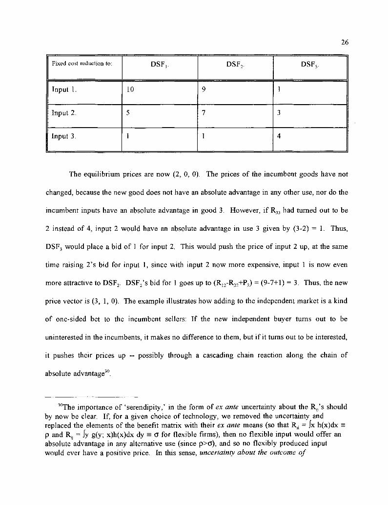
be illustrated with an extension of the earlier numerical example. Suppose that to that system

of two independent inputs, we add a third, and that the three offer cost reductions as in the

following table:

26

Fixed cost reduction to:

Input 1.

Input 2.

Input 3.

DSF^

10

5

1

DSF2.

9

7

1

DSF3.

1

3

4

The equilibrium prices are now (2, 0, 0). The prices of the incumbent goods have not

changed, because the new good does not have an absolute advantage in any other use, nor do the

incumbent inputs have an absolute advantage in good 3. However, if R33 had turned out to be

2 instead of 4, input 2 would have an absolute advantage in use 3 given by (3-2) = 1. Thus,

DSF3 would place a bid of 1 for input 2. This would push the price of input 2 up, at the same

time raising 2's bid for input 1, since with input 2 now more expensive, input 1 is now even

more attractive to DSF2. DSF2's bid for 1 goes up to (Ri2-R22+P2) = (9-7+1) = 3. Thus, the new

price vector is (3, 1, 0). The example illustrates how adding to the independent market is a kind

of one-sided bet to the incumbent sellers: If the new independent buyer turns out to be

uninterested in the incumbents, it makes no difference to them, but if it turns out to be interested,

it pushes their prices up — possibly through a cascading chain reaction along the chain of

absolute advantage30.

30-3The importance of 'serendipity,' in the form of ex ante uncertainty about the Ry's shouldby now be clear. If, for a given choice of technology, we removed the uncertainty andreplaced the elements of the benefit matrix with their ex ante means (so that RH = jx h(x)dx =p and Rjj = \y g(y; x)h(x)dx dy = G for flexible firms), then no flexible input would offer anabsolute advantage in any alternative use (since p>cr), and so no flexibly produced inputwould ever have a positive price. In this sense, uncertainty about the outcome of

27

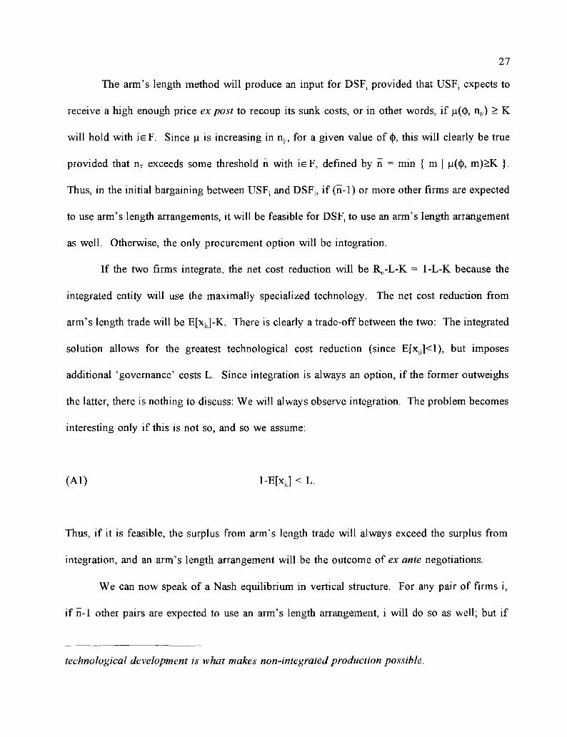
The arm's length method will produce an input for DSF, provided that USF, expects to

receive a high enough price ex post to recoup its sunk costs, or in other words, if u((|>, nF) > K

will hold with ie F. Since u is increasing in nF, for a given value of ((), this will clearly be true

provided that nF exceeds some threshold n with ieF, defined by n = min { m | u{(|), m)>K }.

Thus, in the initial bargaining between USF, and DSF1? if (n-1) or more other firms are expected

to use arm's length arrangements, it will be feasible for DSFX to use an arm's length arrangement

as well. Otherwise, the only procurement option will be integration.

If the two firms integrate, the net cost reduction will be R^-L-K = 1 -L-K because the

integrated entity will use the maximally specialized technology. The net cost reduction from

arm's length trade will be E[xlt]-K. There is clearly a trade-off between the two: The integrated

solution allows for the greatest technological cost reduction (since E f x ^ l ) , but imposes

additional 'governance' costs L. Since integration is always an option, if the former outweighs

the latter, there is nothing to discuss: We will always observe integration. The problem becomes

interesting only if this is not so, and so we assume:

(Al) 1-E[xu] < L.

Thus, if it is feasible, the surplus from arm's length trade will always exceed the surplus from

integration, and an arm's length arrangement will be the outcome of ex ante negotiations.

We can now speak of a Nash equilibrium in vertical structure. For any pair of firms i,

if n-1 other pairs are expected to use an arm's length arrangement, i will do so as well; but if

technological development is what makes non-integrated production possible.

28

fewer than n-1 are expected to integrate, i will integrate. It is immediate that this implies that

the only possible equilibria are nF= 0 and nF= n: complete integration of the sector and universal

use of independent suppliers.

Proposition 7. In a small closed economy (n<n) with utter homogeneity of firms, the only

equilibrium is complete vertical integration. In a large economy (n>n), there are two equilibria:

Complete integration and universal use of independent suppliers.

This highlights a point about the transactions-cost approach that does not appear to be

widely acknowledged: It implies a kind of strategic complementarity in integration decisions.

A larger number of firms using independent supply implies a wider use of flexible technology,

hence a thicker secondary market, and thus makes it more attractive for any given firm to use

independent supply. An immediate consequence is that two otherwise identical economies in

isolation from each other can evolve completely different 'industrial systems' or 'industrial

cultures', one strictly more efficient than the other. This outcome bears a resemblance to

descriptions of national differences in sourcing strategies and particularly the contrast between

the highly integrated 'fordist' model of Western economies and the striking predominance of

outsourcing in Japanese industry as compared to other economies, which many observers appear

to regard as an inherently more efficient sourcing system (for example, Nishiguchi (1994), Gertler

(1991), and The Economist (1991)). In addition, it carries with it the implication that despite this

inefficiency of the integrated outcome, no single firm in the vertically integrated economy would

wish to switch procurement methods: The secondary market would be too thin to make it

29

practical.

The open economy version of this model is then straightforward to analyze. We must

now write the unintegrated USF's expected revenue as u(<j>, t, nF, n r) , where nF, is the number

of unintegrated firms in the other country, to take account of the fact that R is a decreasing

function of t if i<n and j>n or vice versa. The parameter 't' could be either a tariff or transport

costs, or possibly extra transactions costs imposed by cross-border regulation. Whatever the

interpretation, we will call 'globalization' a reduction in 't,' where the initial value will be taken

as a sufficiently high value that in effect the two economies act as if closed. If we define an

economy as 'small', 'medium' or 'large' depending on whether n<n/2, n/2<n<n, or n>n, then it

is clear that for two small economies, globalization will have no effect on vertical structure (since

whatever value t takes, the only equilibrium will be integration). However, in the other two cases

it can have significant effects:

Proposition 8. In the case of utter homogeneity of firms, a sufficient globalization between

medium-sized countries will make the more efficient arm's length equilibrium possible in both

economies. It would not be possible in either economy without globalization.

Clearly, if t falls by enough, the above reasoning for the closed economy case will apply

to the combined economies of the two countries. Thus, the finding that the only equilibria

involved all firms acting in the same way applies as well:

Proposition 9. Whatever the size of the economies concerned, in the case of utter homogeneity

30

of firms, with a sufficient globalization any equilibrium will involve complete convergence of

the vertical structure of the two economies.

5. Industry Equilibrium: The case of wide diversity.

The above homogeneity assumption ought not to be taken too literally, since in practice

it certainly is not true that every single business enterprise within an industry in a given country

does business in exactly the same way. The reason is plausibly that there are some ex ante

differences between firms, for example in their scope for flexibility. Thus, suppose that within

each country each firm has a different value for (j . Let the firms in each country be ordered in

descending order of §{. Again, begin with the closed economy case. We can write the expected

payoff of an unintegrated supplier i as:

, F) = E[PJ.

This time, naturally, the ex ante payoff can differ between firms, and further not only the number

but also the identities of the firms in the unintegrated set F will matter. Not surprisingly, the

expected revenues of an unintegrated firm with a large scope for flexibility will be greater, ceteris

paribus, than those for a firm with less flexibility. This can be seen by considering two firms,

i and j , with ( = fy initially, and noting how their payoffs change with an increase in ((>,.

31

Proposition 10. If i, j e F and i^j, then:

^i!>^>o.

Proof: See Appendix.

Because the payoff to a higher ^ independent USF will be greater than that of a lower

(j), USF, in any Nash equilibrium pattern of vertical structure, F must be composed of an unbroken

sequence of firms from i=l up to and including a threshold firm, say fi, with u((j)fi, {I,-, fi}) > K

but u((j>fi+1, {1,-, n+1}) < K. If u*(i) = n(<j)p {1,..., i}) is a strictly decreasing function of i, there

is only one such fi, and hence one equilibrium. This will clearly be so if ( falls sufficiently fast

in i; here we assume that it does.

In the open economy case, USFj's expected revenue can be written

u ^ , t, (l,...n), {l,...n'}), where fi' is the number of unintegrated firms in country II. For any t

and n', we can find the value of ii consistent with equilibrium in country I. This gives a kind

of country I 'reaction function' (abusing the term somewhat, since each firm pair in country I acts

independently). Since a rise in n' shifts the function u up, this 'reaction function' necessarily

slopes upward. Once again, strategic complementarity is in evidence in integration decisions.

The same argument works for country II, and the two 'reaction functions' can be combined to

find the equilibrium number of independent suppliers (fi, n') in the two countries. This is

demonstrated in Figure 3, under the assumption:

(A2) u(( 1+1; {!,..., i+l}, {n+1,..., n+i'+l}) < u ^ ; {!,..., i},

32

for all i, i'<n. This is the meaning of the assumption of 'wide diversity' between business firms.

It implies that u ^ , {1,..., i+1}, {n+1,..., n}) slopes downward in i, but further that each country's

'reaction function' never has a slope exceeding unity. This is equivalent to so-called 'stability

assumptions' in simple oligopoly models.

Globalization unambiguously raises the incidence of independent supply in both countries,

moving the world economy from point A to point B. This leads to a welfare improvement in

both countries, because of Al.

Finally, note that under these conditions there is a sense in which outsourcing practices

are internationally 'contagious.' If country II undergoes an exogenous change in technology so

that each of its firms now has a greater scope for specialization (and so ()), goes up for each of

its firms), that will lead to a rise in its incidence of outsourcing for any given country I outcome.

This can be represented as the broken curve in Figure 3, a shift of country IPs 'reaction

function.' But this of course stimulates a greater use of outsourcing in country I, and this

reinforces the additional popularity of

outsourcing in country II. Thus, both

countries depend to a greater extent than

before on independent suppliers, with the final

outcome at point C. It should be remembered

that at no time does any trade occur between

these two countries at all: A change in

contracting behaviour in one country affects

the other through the thickness of the implicit

I a

o Country II's'reaction function.'

Country I's 'reaction function.

Indedpendent suppliers in country I, n.

Figure 3: International Equilibrium Under 'Wide Diversity.'

33

secondary market for inputs, thus changing bargaining power. Nonetheless, the process of

'globalization' has had substantial real effects in both countries.

6. Possible Extensions.

The object here has been to show that some simple ideas from industrial organization can

readily to brought into an international context, and offer some promise as a framework for

analyzing the relationship between international openness and vertical structure. In particular,

the central point has been the role of a rise in market 'thickness' resulting from greater openness.

To allow for greater focus on this one effect, the model has been extremely simplified. Here we

will discuss a few directions in which assumptions could be relaxed or altered.

First, there is no particular reason to cling in general to the two extremes of 'utter

homogeneity' and 'wide diversity.' Once those two cases are understood, it is straightforward

to extend the analysis to any intermediate case. The key result of strategic complementarity in

integration decisions, and the finding that the set of non-integrated firms will be the ones with

the highest values of (j),, will still hold. A case of particular interest would be the case in which

the function u*(i) = \i(fo {l,...,i}) has a value greater than K for i=l, falls below K as i rises, then

crosses K twice more as i rises to n. In this case, we have 'highly integrated' and 'highly

unintegrated' equilibria, neither of which is a corner. Thus, there is no reason in general to insist

that multiple equilibria must go hand in hand with a corner solution.

Second, although the appeal of the low-price equilibrium of the price game compared to

the other equilibria seems strong, some may be interested in the consequences of other equilibria.

34

The only other one that seems at all focal is the 'high-price' equilibrium. In this equilibrium (in

the limit as £—»0), the price of input i is given by F1 = max^R^}, or, in the most naive sense,

the value of its best alternative use31. It is straightforward that this reproduces every qualitative

result, mutatis mutandis, in Propositions 2, 3, 6, 8, 9, and 10 (with the exception that a rise in

<k will now increase only the price of input i). Thus, the main economic consequences of the

analysis will be unchanged. However, note that some odd features will be present; aside from

those already mentioned, note that even integrated firms, with their maximally specialized inputs

in hand, will bid positive sums for other firm's inputs, in which they have no interest.

More broadly, one may wish to depart from the Bertrand-type price determination

structure. It may be of interest to examine Walrasian prices, for example. This turns out not to

give any greater generality, however. Because the First Welfare Theorem will be satisfied (ex

post) by such an equilibrium, the allocation of the inputs will be the same as they are in the

bidding equilibrium studied above. Further, using this fact, it is easy to show that the set of

Walrasian price vectors, and the set of price vectors supportable by Nash equilibria of the above

price game, are one and the same. Using results from Giil and Stacchetti (1996), it is easy to

show that the lowest-price Walrasian equilibrium is given by the ODB price vector studied in the

text.

It may be of interest to examine bargaining versions of the model. Perhaps the simplest

way of formulating bargaining in this setting is to allow DSF, and XJSF1 to engage in Nash

bargaining once the input is ready; if the bargaining breaks down, they walk away from the table

31This is supported as a Nash equilibrium by b1} = [RJ" if j^ i and btl = max^fyj+e. Asnoted above, this involves firms making positive, but losing, bids which they strictly prefer tolose.

35

irrevocably and seek other partners; if they find willing partners, they follow Nash bargaining

with them and the game ends. The payoffs from the second (potential) stage of bargaining form

the threat point of the first stage of bargaining. The Appendix shows that this framework

provides conclusions qualitatively identical to the main ones of the text. Extensions to other

bargaining frameworks, including non-cooperative approaches, may be of some interest, as may

approaches that involve the Shapley value.

The relaxation of conditions ensuring condition (1) may be of some interest. If there is

a possibility that some input other than the one designed for DSF, has its socially most efficient

use with DSF13 then we may see 'downsizing' at some times taking the form of 'firing' one's

original input supplier (in other words, not purchasing its input). Thus, although welfare

enhancing, globalization may fail to be ex post Pareto improving. Further, in such a formulation

there would be a second interesting source of welfare benefit from market 'thickening': It would

raise the expected value of a match. In the current model, the expected surplus generated by an

equilibrium match between a USF and a DSF is always E[RJ; market thickening affects the

distribution of this surplus between the two partners, but not the level of this surplus. However,

if (1) does not hold, both effects will be at work, possibly accentuating the strategic

complementarity of integration decisions.

A further generalization that may be of some interest is the allowance for a wider set of

organizational choices. Aside from complete integration and a pure market approach,

procurement in practice involves partial equity control, quasi-integration, contracts of varying

lengths, forms, and complexities; and reputational solutions. It is speculated here that in a richer

model with some more such options specified, each with its own peculiar costs and constraints,

36

we may see a tendency for a thicker market to lead to relatively less integrated forms within

partially integrated firms, as well as a reduction in the number of totally integrated firms. In

addition, it could be quite interesting to inquire how the form of optimal procurement contracts,

for that portion of firms using them, is affected by the sort of general equilibrium effects outlined

here. However, this is beyond the scope of this paper.

Appendix.

Proof of Proposition 4.

First, it is simple to see that we can find a value of k satisfying (i) and (ii). Since there

are a finite number of inputs, for k large enough (ii) must be violated; choose the largest k such

that it is not. For this k, z(j) = z(k+l) for some j<k. Suppose that j<k. Then (Pz(]), PZ(j+i>-'PZ(k))

are all strictly positive (since XQ; P) = j if and only if P- = 0). Thus, from (4),

However, since z(j) = z(k+l), this implies that Iffl=z(a,.,z(k)[Rz(ni)z(m+1)- Rz(in+i)z(m+i)] = 0. However,

this sum can be written as:

which, since z(j) = z(k+l) is negative by (1). This is a contradiction; thus, j=k. By definition

of j , this means that z(k) = z(k+l), but by construction of the z's, this means that A,(z(k); P) =

z(k). But since A,(j; P) = j if and only if Pj= 0, this implies that Pz(k) = 0. Thus, k satisfies (i)

and (ii).

Having established that, (iii) follows by mechanical application of (4). QED.

(Appendix.) 2

Proof of Proposition 5.

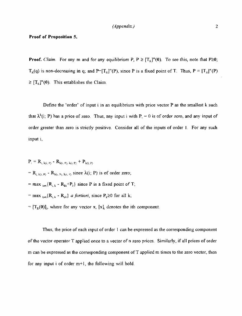
Proof. Claim. For any m and for any equilibrium P, P > [TR]m(0). To see this, note that P>0;

TR(q) is non-decreasing in q; and P=[TR]m(P), since P is a fixed point of T. Thus, P = [TR]m(P)

> [TR]m(0). This establishes the Claim.

Define the 'order' of input i in an equilibrium with price vector P as the smallest k such

that ?ik(i; P) has a price of zero. Thus, any input i with P, = 0 is of order zero, and any input of

order greater than zero is strictly positive. Consider all of the inputs of order 1. For any such

input i,

M = -K-i, Hi; P) " RA(i; P), X<i; P) ~*~ "x<i; P)

= Ri, /to, p) - Rx<i; P), m; P) s i n c e ^(i; p ) i s o f order zero;

= max k^i{Ri)k - Rkk+Pk} since P is a fixed point of T;

= max ^{Ri^ - Rkkl a fortiori, since Pk^0 for all k;

= [TR(0)L> where for any vector x, [x], denotes the ith component.

Thus, the price of each input of order 1 can be expressed as the corresponding component

of the vector operator T applied once to a vector of n zero prices. Similarly, if all prices of order

m can be expressed as the corresponding component of T applied m times to the zero vector, then

for any input i of order m+1, the following will hold.

(Appendix.) 3

i ~ Ri, Mi; P) " R^(i; P), MK P) + *<i; P)

max ^ { R ^ - R^ + Pk} since P is a fixed point of T;

max k^{Ri)k - R^ + [[TR]m(0)]k} (a fortiori, since Pk>[[TR]m(O)]k for all k by the above Claim);

Thus, the reasoning can be applied to all m by induction. Observing that

[[TR]m(0)]k=[[TR]r(0)]k for all m and r greater than or equal to the order of k, and that each input

is of order n-1 or less, completes the proof. QED.

Proof of Proposition 10.

Consider a realization of R and the price vector P that results. Holding all else constant, we may

write both as a function of (j : R(<|>1) and P ^ ) . Note that BR^/B^ takes a value of xkm if k =

i and m ^ i, and zero otherwise. Assume that PCc)),) is such that there exists a neigborhood S

around P ^ ) such that for all P'e S, and for any input m, A,(m; P') = A,(m; P^,)) (in other words,

there are no tying bids). This will be true with probability 1. By Proposition 4, P- will be

affected by <)>, if and only if there is a chain of runner-up bidders leading from input j to input

i, and P, > 0. Thus, if P1 = 0, dPfify = 0 and BP/Bifc = 0. If P, > 0, then by Proposition 4,

dP/d^ = Xi .p). Further, if P>0, then BPj/BcJ), takes a value of xt^p) if there is a chain of

runner-up bidders going from j to i, and zero otherwise. Thus, if we denote by A(i, j) the set of

realized values of R such that P1 > 0 and for some m > 0, i = XmQ; P); and denote by B(i) the

set of realized values of R such that P, > 0, then:

(Appendix.)

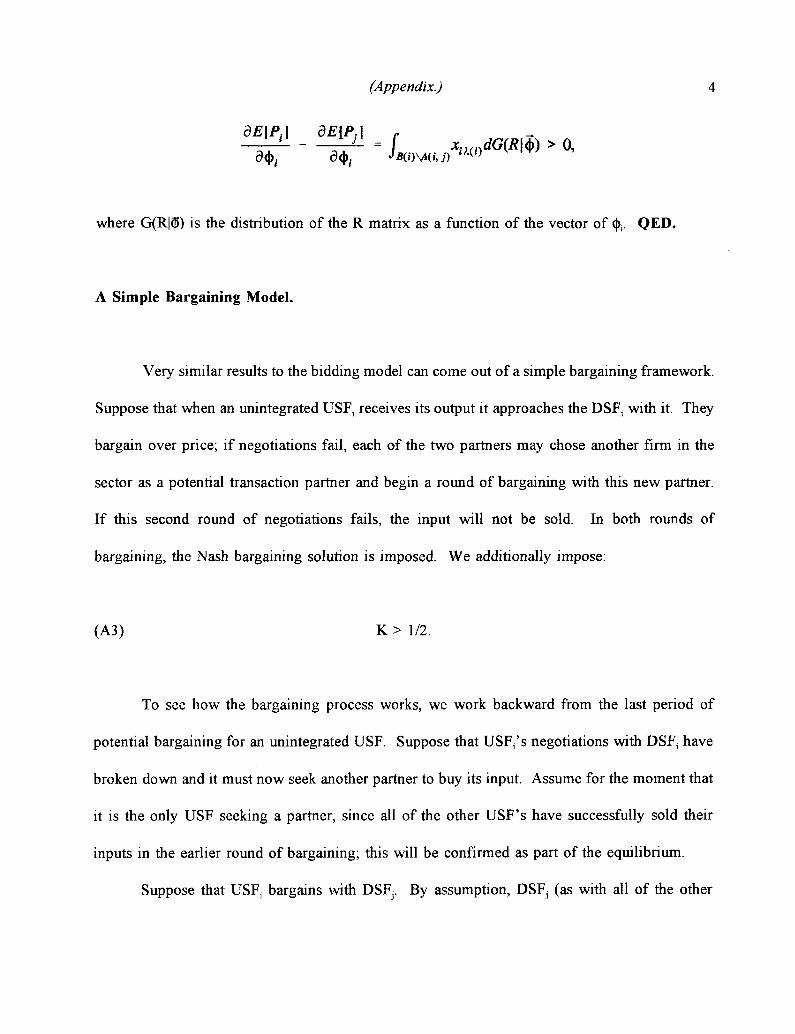
dE[P(] dE[Pj]

where G(R|$) is the distribution of the R matrix as a function of the vector of <j)r QED.

A Simple Bargaining Model.

Very similar results to the bidding model can come out of a simple bargaining framework.

Suppose that when an unintegrated USFa receives its output it approaches the DSF, with it. They

bargain over price; if negotiations fail, each of the two partners may chose another firm in the

sector as a potential transaction partner and begin a round of bargaining with this new partner.

If this second round of negotiations fails, the input will not be sold. In both rounds of

bargaining, the Nash bargaining solution is imposed. We additionally impose:

(A3) K > 1/2.

To see how the bargaining process works, we work backward from the last period of

potential bargaining for an unintegrated USF. Suppose that USF,'s negotiations with DSFX have

broken down and it must now seek another partner to buy its input. Assume for the moment that

it is the only USF seeking a partner, since all of the other USF's have successfully sold their

inputs in the earlier round of bargaining; this will be confirmed as part of the equilibrium.

Suppose that USFt bargains with DSFr By assumption, DSFj (as with all of the other

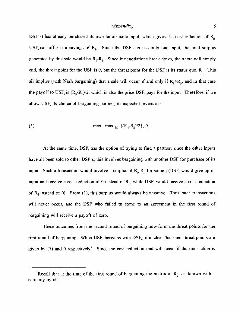
(Appendix.) 5

DSF's) has already purchased its own tailor-made input, which gives it a cost reduction of Rjr

USFj can offer it a savings of R,r Since the DSF can use only one input, the total surplus

generated by this sale would be R -R . Since if negotiations break down, the game will simply

end, the threat point for the USF is 0, but the threat point for the DSF is its status quo, R . This

all implies (with Nash bargaining) that a sale will occur if and only if R1J>R3J, and in that case

the payoff to USF1 is (R-R^)/^, which is also the price DSFj pays for the input. Therefore, if we

allow USFj its choice of bargaining partner, its expected revenue is:

(5) max {max {j} {(R^-R^/2}, 0}.

At the same time, DSF, has the option of trying to find a partner; since the other inputs

have all been sold to other DSF's, this involves bargaining with another DSF for purchase of its

input. Such a transaction would involve a surplus of R -R^ for some j (DSFj would give up its

input and receive a cost reduction of 0 instead of RJJ5 while DSFj would receive a cost reduction

of Rjt instead of 0). From (1), this surplus would always be negative. Thus, such transactions

will never occur, and the DSF who failed to come to an agreement in the first round of

bargaining will receive a payoff of zero.

These outcomes from the second round of bargaining now form the threat points for the

first round of bargaining. When USFj bargains with DSF15 it is clear that their threat points are

given by (5) and 0 respectively1. Since the cost reduction that will occur if the transaction is

Recall that at the time of the first round of bargaining the matrix of R^'s is known withcertainty by all.

(Appendix.) 6

completed is R11? the surplus from the transaction is R^ minus the value in (5); by (1), this is

always positive, so the transaction will occur. The price that USFt is paid for the input is:

(6)U + max

Thus, if we back up to the time at which the USF makes its decision as to whether or not to

proceed with the investment, we can calculate its expected revenue. Note that if the USF has

chosen maximal specialization, since Ry= 0 for j^ i , (6) takes a value of Rtl/2 < 1/2. By A3, this

is less than the cost of producing the input, so we know that the unintegrated USF would never

proceed with production of the input using the maximally specialized technology. Further, in

calculating (6) we can ignore any DSF that has chosen the maximally specialized technology,

since for such a firm R]J=1 and so R - RJJ

<0. Thus, we restrict attention to the case of the

flexible technology strategy, in which case the expected revenue to USFt is given by:

(7) = E 2 p +

where 3> is the set of USF's who have chosen the flexible technology strategy, no is the number

of USF's in this set, and the expectation is taken with respect to the random variables x for je<£.

Clearly, since adding one more firm with flexible technology simply adds one more value of

(Appendix.) 1

R-Rjj to the list from which a maximum is selected, (|> is increasing in n^. Thus, Proposition 6

carries over to this bargaining model. The other propositions follow similarly.

Bibliography.

Alchian, Armen A. and Harold Demsetz (1972). "Production, Information Costs, andEconomic Organization," American Economic Review 62: pp. 777-95.

Baba, Yasunori, Shinji Takai, and Yuji Mizuta (1995). "The Japanese software industry: the'hub structure' approach," Research Policy 24, pp. 473-86.

Bamford, James (1994). "Driving America to tiers" Financial World 163:23 (November 8),pp. 24-27.

Bardi, Edward J., and Tracey, Michael (1991). "Transportation Outsourcing: A Survey of USPractices" International Journal of Physical Distribution & Logistics Management,21:3, pp. 15-21.

Bank Systems & Technology (1991). "Technology Survey '91: Is Outsourcing About to Makethe Big Time?" 28:9 (September), pp. 49-52.

Bolton, Patrick and Michael D. Whinston (1993). "Incomplete Contracts, Vertical Integration,and Supply Assurance," Review of Economic Studies 60, pp. 121-48.

Brock, Gerald (1989). "Dominant Firm Response to Competitive Challenge: PeripheralManufacturers' Suit Against IBM (1979-1983)." Chapter 6 of Kwoka, John E. Jr. andLawrence J. White (ed.) (1989). The Antitrust Revolution (1st edition). New York:HarperCollins.

Buxbaum, Peter (1994). "Focusing on third parties," Distribution. 93:12. (November),pp.60-65.

Calvo, Guillermo A. and Stanislaw Wellisz (1978). "Supervision, Loss of Control, and theOptimum Size of the Firm," Journal of Political Economy 86:5 (October), pp. 943-52.

Cremer, Jacques (1996). "Arm's Length Relationships," Quarierly Journal of EconomicsCX:2 (May), pp. 275-95.

Economist (1991). "Manufacturing - The Ins and Outs of Outing," 320:7722 (August 31,1991). pp. 54,56.

Gardner, Elizabeth (1991). "Going On Line with Outsiders," Modern Healthcare 21:28, July15, 1991. p. 35-47.

Gertler, Meric S. (1991). "Canada in a High-Tech World: Options for Industrial Policy," inDaniel Drache and Meric S. Gertler, The New Era of Global Competition: State Policyand Market Power. Montreal: McGill/Queen's University Press.

Grossman, Sanford J. and Oliver D. Hart (1986). "The Costs and Benefits of Ownership: ATheory of Vertical and Lateral Integration." Journal of Political Economy 94:4, pp.692-719.

Gul, Faruk and Ennio Stacchetti (1996). "Walrasian Equilibrium without Complementarities,"Mimeo.

Hart, Oliver and John Moore (1990). "Property Rights and the Nature of the Firm," Journalof Political Economy 98:6, pp. 1119-58.

Hart, Oliver and Jean Tirole (1990). "Vertical Integration and Market Foreclosure."Brookings Papers: Microeconomics 1990, pp. 205-286.

Joskow, P. (1987). "Contract Duration and Relation-specific Investments: Empirical Evidencefrom Coal Markets." American Economic Review 77:1 (March), pp. 168-85.

Klein, Benjamin, Robert G. Crawford, and Armen A. Alchian (1978). "Vertical Integration,Appropriable Rents, and the Competitive Contracting Process," The Journal of Lawand Economics XXI, (October), pp. 297-326.

Masten, Scott E. (1984). "The Organization of Production: Evidence from the AerospaceIndustry," Journal of Law and Economics XXVII (October), pp. 403-17.

Maynard, Micheline (1996). "Study: Outsourcing gives edge," USA Today, June 25, 1996, p.B2.

Monteverde, Kirk and David J. Teece (1982). "Supplier Switching Costs and VerticalIntegration in the Automobile Industry," Bell Journal of Economics 13:1 (Spring), pp.206-13.

Morris, Jonathan (1991). "A Japanization of Canadian Industry?" in Daniel Drache andMeric S. Gertler, The New Era of Global Competition: State Policy and MarketPower. Montreal: McGill/Queen's University Press.

Nishiguchi, Toshihiro (1994). Strategic Industrial Sourcing: The Japanese Advantage. NewYork: Oxford University Press.

Noldeke, Georg and Klaus M. Schmidt (1995). "Option Contracts and Renegotiation: ASolution to the Hold-Up Problem," The RAND Journal of Economics 26:2 (Summer),pp. 163-79.

Numagami, Tsuyoshi (1996). "Flexibility trap: a case analysis of U.S. and Japanesetechnological choice in the digital watch industry," Research Policy 25, pp. 133-62.

Ordover, Janusz A., Garth Saloner and Steven C. Salop (1990). "Equilibrium VerticalForeclosure." American Economic Review 80:1, pp. 127-142.2.

Perry, Martin K. (1989). "Vertical Integration," in Richard Schmalensee and Robert Willig(ed.), Handbook of industrial organization, New York: North-Holland, pp. 135-82.

Rogerson, William P. (1992). "Contractual Solutions to the Hold-Up Problem," Review ofEconomic Studies 59, pp. Ill-19A.

Spencer, Barbara J., and Ronald W. Jones (1991). "Vertical Foreclosure and InternationalTrade Policy," Review of Economic Studies 58 (January), pp. 153-70.

(1992). "Trade and Protection in Vertically Related Markets," Journal ofInternational Economics 32 (February), pp. 31-55.

Telser, Lester C. (1981). "Why There Are Organized Futures Markets," Journal of Law andEconomics 24, pp. 1-22.

Vincenti, Walter, G. (1994). "Variation-selection in the innovation of the retractable airplanelanding gear: the Northrop 'anomaly,'" Research Policy 23, pp. 575-82.

Williamson, Oliver (1971). "The Vertical Integration of Production: Market FailureConsiderations," American Economic Review LXI:2 (May), pp. 112-23.

(1989). "Transaction Cost Economics." Chapter 3 in RichardSchmalensee and Robert Willig (ed.), Handbook of industrial organization, New York:North-Holland, pp. 135-82.

1995-1996 Discussion Paper Series

Department of EconomicsColumbia University

1022 International Affairs Bldg.420 West 118th Street

New York, N.Y., 10027

The following papers are published in the 1995-96 Columbia University Discussion Paper serieswhich runs from early November to October 31 of the following year (Academic Year).

Domestic orders for discussion papers are available for purchase at the cost of $8.00 (U.S.) Perpaper and $140.00 (US) for the series.

Foreign orders cost $10.00 (US) per paper and $185.00 for the series.

To order discussion papers, please write to the Discussion Paper Coordinator at the above addressalong with a check for the appropriate amount, made payable to Department of Economics,Columbia University. Please be sure to include the series number of the requested paper when youplace an order.

1995-96 Discussion Paper Series

9596-01 Protectionist Response to Import Competition in Declining Industries by: J. ChoiReconsidered

9596-02 New Estimates on Climate Demand: Evidence from Location Choice

9596-03 Enforcement by Hearing

9596-05 Simplification, Progression and a Level Playing Field

9596-06 The Burden of Proof in Civil Litigation

9596-07 Market Structure and the Timing of Technology Adoption

9596-08 The Emergence of the World Economy

9596-09 The Global Age: From a Skeptical South to a Fearful North

9596-10 A Conformity Test for Cointegration

9596-11 Identification and Kullback Information in the GLSEM

9596-12 Informational Leverage and the Endogenous Timing of ProductIntroductions

9596-13 Changes in Wage Inequality

9596-14 The Design of Monte Carlo Experiments for VAR Models

9596-15 A Topological Invariant for Competitive Markets

9596-16 Topology and Invertible Maps

9596-17 Smooth Infinite Economies

by: M. Cragg

M. Kahn

by: C. Sanchirico

9596-04 Preferential Trading Areas and Multilateralism: Strangers, Friends or by: J. BhagwatiF o e s ? A. Panagariya

by: W. Vickrey

by: C. Sanchirico

by: J. Choi

M. Thum

by: R. Findlay

by: J. Bhagwati

by: P. Dhrymes

by: P. Dhrymes

by: J. Choi

by: J. Mincer

by: P. Dhrymes

by: G. Chichilnisky

by: G. Chichilnisky

by: G. Chichilnisky

1995-96 Discussion Paper Series

9596-18 Measuring Neighborhood Investments: Urban Quality of Life by: D. DipasqualeExpenditures by Race M K h

9596-19 The Silver Lining of Industrial Decline: Rust Belt Manufacturing's by: M. KahnImpact on Particulates

9596-20 Education's Role in Explaining Diabetic Health Investment Differentials by: M. Kahn

9596-21 Limited Arbitrage and Uniqueness of Market Equilibrium by: G. Chichilnisky

9596-22 A Probabilistic Model of Learning in Games by: C. Sanchirico

9596-23 Minimal Inclusive Sets in Special Classes of Games by: C. Sanchirico

9596-24 'Globalization' and Vertical Structure by: J. McLaren

9596-25 Corruption, Black Markets and the Fiscal Problem in LDC's: Some by: J. McLarenRecent Findings

9596-26 Black Markets and Optimal Evadable Taxation by: J. McLaren