1

HomER Hemodynamic Evoked Response

NIRS data analysis GUI

Program User’s Guide Stand-alone executable version

(Version 4.0.0)

Release July 28th, 2005

Written by:

Theodore Huppert, M.Sc. David A. Boas, Ph.D.

Photon Migration Imaging Lab Massachusetts General Hospital/CNY

Charlestown, MA 02139

2

Copyright 2005: Massachusetts General Hospital End-User Licensing Agreement ("EULA") for HomER: IMPORTANT- READ CAREFULLY: 1. GRANT OF LICENSE. This EULA grants the licensee the following rights: Software. The licensee may install one copy of HomER on a single computer. Network Use. The licensee may use HomER over an internal network, and the licensee may distribute HomER to other computers over an internal network. Documentation. The licensee may make a copy of the documentation for internal use only. This EULA grants the licensee a nonexclusive, nontransferable, no-cost, royalty free right to use the HomER for licensee's internal, non-commercial, non-clinical, academic research purposes only, under the terms of this agreement. 2. LIMITATIONS Academic Version. HomER can only be used by Colleges, Universities, and other Non-Profit Research Organizations for research only. Colleges, Universities, and other Non-Profit Research Organizations may not use HomER in any commercial arrangement to any third-parties when payments are made for services rendered, either directly, or indirectly, when the functionality contained within HomER has been used. For-profit organizations and companies are explicitly prohibited from using this software for any purposes. Rental. The licensee may not rent or lease HomER. Commercial Use. The licensee may not charge anyone for any activity that uses HomER. For example, the licensee may not charge for segmentation, quantification, and/or corticalsurface reconstruction using HomER. The licensee cannot charge others for installation of the software, nor can they pay any entity, other than a full-time employee, to install and operate the software. The licensee may not incorporate HomER or any of its parts into any commercial code or product of any kind. Software Transfer. The licensee may not transfer HomER to any third party. Clinical Use: This software may not and should never be used for clinical purposes. Software used for clinical purposes may require regulatory documentation and associated filings. Termination. 3. COPYRIGHT and TRADEMARKS. HomER. All title and copyrights in and to HomER (including but not limited to any code, documentation, images, text or data) are owned by The General Hospital Corporation doing business as Massachusetts General Hospital. HomER is protected by copyright laws and international copyright treaties, as well as other intellectual property laws and treaties. HomER is licensed, not given away or sold. PMI toolbox. Parts of this software are based on the PMI toolbox software copyrighted by The Massachusetts General Hospital and John Stott. The original license terms of the PMI toolbox software distribution is included in the file docs 4. NO SUPPORT OR WARRANTY. HomER is provided with no support whatsoever. The General Hospital Corporation may, at their sole discretion, provide bug reports or upgrades at www.nmr.mgh.harvard.edu/DOT, The General Hospital Corporation do not have any obligation to notify users of this occurring. HomER may contain in whole or in part pre-release, untested, or not fully tested works. HomER may contain errors that could cause failures or loss of data, and may be incomplete or contain inaccuracies. LICENSEE expressly acknowledges and agrees that use of HomER, or any portion

3

thereof, is at LICENSEE's sole and entire risk, and that HomER is an experimental program. HomER is provided "AS IS" and without warranty, upgrades or support of any kind. THE GENERAL HOSPITAL CORPORATION EXPRESSLY DISCLAIMS ALL WARRANTIES AND/OR CONDITIONS, EXPRESS OR IMPLIED, INCLUDING, BUT NOT LIMITED TO, THE IMPLIED WARRANTIES AND/OR CONDITIONS OF MERCHANTABILITY OR SATISFACTORY QUALITY AND FITNESS FOR A PARTICULAR PURPOSE AND NONINFRINGEMENT OF THIRD PARTY RIGHTS. THE GENERAL HOSPITAL CORPORATION DOES NOT WARRANT THAT THE FUNCTIONS CONTAINED IN HOMER WILL MEET LICENSEE'S REQUIREMENTS, OR THAT THE OPERATION OF HOMER WILL BE UNINTERRUPTED OR ERROR-FREE, OR THAT DEFECTS IN HOMER WILL BE CORRECTED. NO ORAL OR WRITTEN INFORMATION OR ADVICE GIVEN BY THE GENERAL HOSPITAL CORPORATION OR A CORTECHS LABS, INC. AUTHORIZED REPRESENTATIVE SHALL CREATE A WARRANTY OR IN ANY WAY INCREASE THE SCOPE OF THIS WARRANTY. LICENSEE ACKNOWLEDGES THAT HOMER IS NOT INTENDED FOR CLINICAL USE AND SHOULD NOT BE USED FOR DIAGNOSIS, TREATMENT PLANNING, OR ANY OTHER CLINICAL PURPOSE. 5. LIMITATION OF LIABILITY. UNDER NO CIRCUMSTANCES SHALL THE GENERAL HSOPITAL CORPORATION BE LIABLE FOR ANY INCIDENTAL, SPECIAL, INDIRECT OR CONSEQUENTIAL DAMAGES ARISING OUT OF OR RELATING TO THIS LICENSE OR LICENSEE'S USE OR INABILITY TO USE HOMER, OR ANY PORTION THEREOF, whether under a theory of contract, warranty, tort (including negligence), products liability or otherwise. 6. MISCELLANEOUS. U.S. Government End Users. The Covered Code is a "commercial item" as defined in FAR 2.101. Government software and technical data rights in the Covered Code include only those rights customarily provided to the public as defined in this License. This customary commercial license in technical data and software is provided in accordance with FAR 12.211 (Technical Data) and 12.212 (Computer Software) and, for Department of Defense purchases, DFAR 252.227-7015 (Technical Data -- Commercial Items) and 227.7202-3 (Rights in Commercial Computer Software or Computer Software Documentation). Accordingly, all U.S. Government End Users acquire Covered Code with only those rights set forth herein. Waiver; Construction. Any law or regulation which provides that the language of a contract shall be construed against the drafter will not apply to this License. Quebec. Where LICENSEEs are located in the province of Quebec, Canada, the following clause applies: The parties hereby confirm that they have requested that this License and all related documents be drafted in English. Les parties ont exigé que le présent contrat et tous les documents connexes soient rédigés en anglais. Authority. The person submitting this registration warrants that he/she has the authority to bind to this Agreement the party which he/she represents.

Table of Contents: Overview of features:

4

Appendix: Quick overview of functions - - - - - - - - - - - - - - - - 5 Chapter 1: Download and Installation - - - - - - - - - - - - - - - - 21 Chapter 2: Data format and Preprocessing - - - - - - - - - - - - - - - - 24 Chapter 3: Starting an analysis session - - - - - - - - - - - - - - - - 28 Chapter 4: Filtering the data - - - - - - - - - - - - - - - - 31 Chapter 5: Averaging the stimulus response - - - - - - - - - - - - - - - - 39 Chapter 6: Image reconstructions - - - - - - - - - - - - - - - - 45 Chapter 7: Data display and Export - - - - - - - - - - - - - - - - 49 Chapter 8: Statistical Analysis - - - - - - - - - - - - - - - - 52 Chapter 9: Region-of-interest Analysis - - - - - - - - - - - - - - - - 53 Chapter 10: Sample Data - - - - - - - - - - - - - - - - 54 Simple_probe.nirs - - - - - - - - - - - - - - - - 54 OverlappingProbe.nirs - - - - - - - - - - - - - - - - 59 Physiology_Probe.nirs - - - - - - - - - - - - - - - - 65 Appendix I: HomER data structure - - - - - - - - - - - - - - - - 69 Appendix II: Technical reports - - - - - - - - - - - - - - - - 72 Filtering Code: DOTFilter - - - - - - - - - - - - - - - - 72 HomERFilt - - - - - - - - - - - - - - - - 79 PCAFilter - - - - - - - - - - - - - - - - 83 PCA_Filter_dConc - - - - - - - - - - - - - - - - 86 Averaging Code: AverageHRF - - - - - - - - - - - - - - - - 90 DeconvolveHRF - - - - - - - - - - - - - - - - 95 HRFStatistics - - - - - - - - - - - - - - - - 100

Overview of HomER features:

5

HomER is a data analysis program written by the PMI lab at MGH for the purpose of quick, reliable, and user-friendly analysis of near-infrared spectroscopy. Comments and suggestions are always welcome and should be sent to T. Huppert (thuppert@nmr.mgh.harvard.edu). Acknowledgements: HomER is developed under funds from the National Institute of Health (R01-EB002482, P41-RR14075), NCRR, and the MIND institute. T. J. H. is funded by the Howard Hughes Medical Institute Pre-Doctorial program.

Quick Overview of Features:

6

Filtering Filtering tab features:

1) Main Data display window. This window displays the data for the entire experimental time course. Display type is set by items 10) and 11). This window is cleared when multi-file averages are being displayed. Right clicking on this window allows export of the data displayed. Data can also be copied to the clipboard by right-clicking on a displayed data line. The colors of displayed data correspond to the color of the source-detector pair highlighted in window 2 (item 2).

2) Probe Geometry display This window displays the loaded probe geometry. Clicking on the probe positions changes the displayed source-detectors in window 1). The probe is specified by the “SD” variable and loaded with the *.nirs file. Clicking

1 2

3456 7

89

1011

121314

15

16

17

1819 20 21

1 2

3456 7

89

1011

121314

15

16

17

1819 20 21

7

near an optode position will move display to the nearest optode. Clicking on a line will toggle the display of the corresponding source-detector pair. X/Y labels are in centimeters. When lines are toggled off (displayed as dotted lines), they will be discluded from filtering (i.e. PCA analysis) averaging, and image reconstruction. This can be used to remove “noisy” data channels.

3) LP/HP filter settings These fields set the Low and High pass filtering parameters. Values are given in hertz. Invalid cut-off frequencies are skipped with a warning. To skip either filtering step, the filter cut-off should be set to “[]” (empty set). Filter parameters (inc. order, type etc) are specified under item 14). See section 4.2

4) Motion correction PCA filter settings This field specifies the number of principle components (singular values) filtered from the data. This uses a trunctated SVD filter. Eigen-values are displayed by item 9). If only one (1) value is specified, then all wavelengths are filtered together (i.e. both wavelengths are used in same SVD). To filter each wavelength separately, multiple values should be specified. This function operates on the normalized intensity. See section 4.3

5) dOD PCA filter settings This field specifies the number of baseline principle components filtered from the data. Only available if baseline data is present. See section 4.4

6) dConc PCA filter settings This field specifies the number of principle components of concentration filtered from the data. Principle components taken from current file OR baseline (if loaded). Selected by item 8) A value should be specified for each hemoglobin species [oxy-hemoglobin deoxy-hemoglobin] (in that order). See section 4.5

7) Component selection Menu Selects whether the priniple components removed by item 6) are taken from the current file OR baseline file. Only available if baseline data is specified. This also changes the display on item 9) to reflect this selection. See section 4.5.

8) Prune Source-detector list menu Launches measurement list pruning window. See items 72-82). See items 72-82

8

9) View Single-value spectrum Plots the single-value spectrum in a new window. See Section 4.6.

10) Data display choice menu Select which data type to display in window 1). Only raw data is avalaible until filtering is preformed.

11) Wavelength display choice menu Select which wavelength

12) Toggle Zoom control Toggles on/off the zoom control

13) Launch new window display

Launches window with data and average time traces.

14) Filtering Options menu Launches filtering options menu (items 59-71).

15) Show power spectral density Launches new window with plot of the power spectrum of the currently displayed data. Same section 7.5.

16) Display all data Displays color-scale plot of intensity verses channel number in window 1)

17) Probe geometry file Name of probe geometry file if loaded separately from *.nirs file

18) Select Session/Subject

Select the current session(or subject) to analyze (if multiple are open)

19) Select data file Switch between open data files.

20) Mark as Baseline data Mark the current data file (item 19) as a baseline measurement

21) Filtering Menu Tab

Displays filtering options Averaging Tab Features:

9

22) Average data display window Window for display of average data. Data type is specified by items 33-35.

23) HRF pretime edit field Specifies the hemodynamic response pretime (time prior to stimulus) to use in averaging/deconvolution. Specified for currently selcted regressor (item 33). See section 5.5.

24) HRF post-stimulus edit field Specifies the hemodynamic response post-time (time following stimulus) to use in averaging/deconvolution. Specified for currently selcted regressor (item 33). See section 5.5.

25) Calculate Average Preforms calculation of average response. See section 5.7 & 5.8.

26) Preform deconvolution of data

222324

25

26

27

2829

3031 32

333435

36 373839

4041

42

43

222324

25

26

27

2829

3031 32

333435

36 373839

4041

42

43

10

Preforms a deconvolution (rather then a block average) with item 25) See section 5.8.

27) Show stimulus points Displays stimulus points on window 1) See section 5.3.

28) Stimulus thresh-hold Threshold value for pruning “raw” stimulus data. See section 5.1.

29) Minimum ISI Minimum inter-stimulus interval value for pruning “raw” stimulus data. See section 5.1.

30) View original stimulus Plots raw stimulus data on window 1). See section 5.1.

31) Use User-defined stimulus Toggle button to use User-defined stimulus (item 32). See section 5.2.

32) Edit User-defined stimulus Edit field to enter User-defined stimulus points. See section 5.2.

33) Which regressor to display Select which regressor to display data for (if multiple regressors were used). See section 5.6.

34) Select type of data display Select which data trace to display (dOD or dConc).

35) Select Wavelength Select which wavelength to display

36) Display All data

Display all data traces

37) Edit min/max scale Edit the max/min values to scale the display in window 2

38) Set minimum scale

11

Apply minimum scaling to window 2

39) Set Maximum scale Apply maximum scaling to window 2

40) Toggle Zoom on 41) Averaging Options

Launch averaging options window

42) Averaging Tab Display averaging buttons

43) Reset measurement list

Resets measurement list of which source-detectors to include in analysis

12

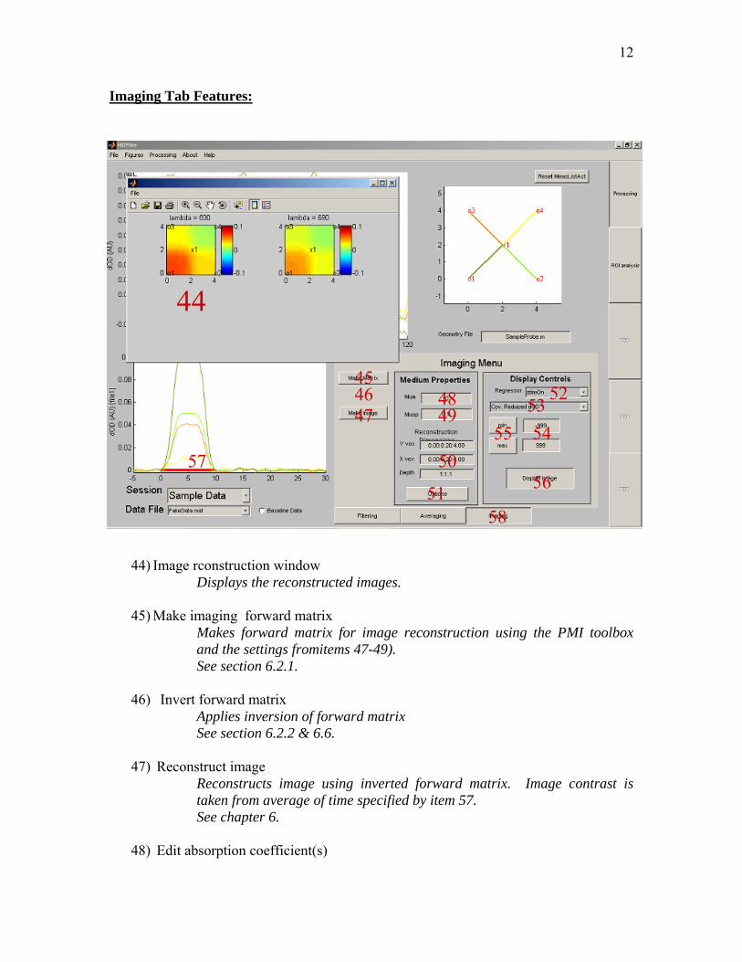
Imaging Tab Features:

44) Image rconstruction window Displays the reconstructed images.

45) Make imaging forward matrix Makes forward matrix for image reconstruction using the PMI toolbox and the settings fromitems 47-49). See section 6.2.1.

46) Invert forward matrix Applies inversion of forward matrix See section 6.2.2 & 6.6.

47) Reconstruct image Reconstructs image using inverted forward matrix. Image contrast is taken from average of time specified by item 57. See chapter 6.

48) Edit absorption coefficient(s)

44

454647

4849

50

5253

51

5455

5657

58

44

454647

4849

50

5253

51

5455

5657

58

13

Specify the baseline absorption coefficient for calculating the forward matrix. If only one value is specified, the same value is used for all wavelengths. See section 6.1.

49) Edit scattering coefficient(s) Specify the baseline reduced scattering coefficient for calculating the forward matrix. If only one value is specified, the same value is used for all wavelengths. See section 6.1

50) Image voxel dimensions These fields allow the user to specify the volume dimensions for image reconstruction. The default settings are based on the probe dimensions. Each direction is specified as [Start Coordinate: step size: End Coordinate]. All values are in centemeters.

51) Imaging options This launches a window with the options for image reconstrunction and display

52) Select which regressor In the case of multiple regressors in the linear regression model, this popup-menu selects which regressor is used in the image reconstruction.

53) Select image display type

Choice between reconstruction a delta-OD, concentration, or contrast-to-noise ratio image. See section 6.3.2.

54) Edit max/min image scale These fields set the maximum/minimum scales for image display. The effects are toggled on/off by item 54).

55) Use image scaling These buttons toggle whether to autoscale or use the image scaling properties specified by 53).

56) Redisplay image If an image has already been reconstructed, this will replot the image in a new window.

57) Select image time window This red bar is used to specify the time window over which to average when displaying an image. This is also used when specifying the t-

14

statistics value(s) for the response. Clicking above the red bar will change its length, while clicking below it will move the initial position. See section 6.3.1.

58) Imaging Tab This selects the imaging options window

Filtering Options menu Measurement Pruning menu

59) Current Absroption spectrum used This displays the partial citation for the currently selcted hemoglobin absorption spectrum.

60) View current absorption spectrum This plots the absoroption spectrum for oxy/deoxy-hemoglobin in a new window according to which absorption spectrum was selected in ite, 60) See section 4.8.

61) Change absorption spectrum This allows one to select which absorption spectrum for hemoglobin is used for the modified Beer-Lambert Law. A user-defined spectrum can also be loaded.

5960 61

62 6364

6566 67

68697071

5960 61

62 6364

6566 67

68697071

7 2 7 37 4 7 5

7 6

7 7 7 87 9 8 0

8 1

8 2

7 2 7 37 4 7 5

7 6

7 7 7 87 9 8 0

8 1

8 2

15

See section 4.8

62) Select type of iirfilter design This allows the user to specify the irrfilter design applied during signal processing. For the Chebshev or elptic filter designs, the tolerances for the pass-band and stop-band are also specified. See section 4.8.

63) Edit filter order This allows the user to specify a higher filter order (default 5) for the signal processing. See section 4.11.

64) View filter charectoristics This create a new window displaying the filter design charectoristics for the signal processing filters. See items 61 & 62. See section 4.11.

65) Add custom filtering step Check this box to include the custom filter step (if loaded). Note: This feature is not available in the stand-alone version. See section 4.10.

66) Load custom filtering function

This allows the user to specify a custom script that gets executed within the signal processing. Note: This feature is not available in the stand-alone version. See section 4.10

67) Name of custom file

This displays the name of the custom filter loaded by 64). Note: This feature is not available in the stand-alone version. See section 4.10

68) DPF correction factor Differential path-length factor to be included in the modified Beer-Lambert law. Defined separately for each wavelength. See section 4.9

69) Include DPF in calculations Check box to include DPF (item 68) in MBBL calculation of hemoglobin Default setting does NOT include this factor. See section 4.9

70) Partial volume corrections

16

Partial volume correction to be included on concentration calculations. Defined separately for each wavelength. See section 4.9.

71) Include partial volume correction to DPF Check box to include partial volume correction (item 70) in MBBL calculation of hemoglobin Default setting does NOT include this factor. See section 4.9

72) Use min intensity criterian in prune If checked, measurements will be excluded if below intensity (set by item 73). See section 4.12.

73) Set minimum intensity Sets minimum intensity for pruning. See section 4.12.

74) Use max intensity criterian in prune If checked, measurements will be excluded if below intensity (set by item 75). See section 4.12.

75) Set maximum intensity Sets maximum intensity for pruning. See section 4.12.

76) View histogram of intensities Displays a histogram of the mean (D.C.) intensities for the data. Useful for desciding the level of pruning.

77) Set maximum source-detector seperation Sets maximum source-detector distance (in cm) for pruning. See section 4.12.

78) Use max SD seperation in prune If checked, measurements will be excluded if the source-detector seperation if greater then this distance [in cm] (set by item 77). See section 4.12.

79) Set minimum source-detector seperation Sets minimum source-detector distance (in cm) for pruning. See section 4.12.

80) Use min SD seperation in prune

17

838485

8687

888990 91

838485

8687

888990 91

92 93

9495

9697

92 93

9495

9697

If checked, measurements will be excluded if the source-detector seperation if less then this distance [in cm] (set by item 77). See section 4.12.

81) View histogram of separations Displays a histogram of the source-detector distances for the data. Useful for desciding the level of pruning. See section 4.12.

82) Apply pruning to data This button applies the settings of 72-81) to the data. Measurements pruned from the dataset appear as dotted lines on the probe geometry (item 2).

See section 4.12.

Averaging Options menu Imaging Options menu

83) Display of currently used regressors This is a list of the currently used regressors for the multiple regressor deconvilution or the list of stimulus variables used for averaging. The default value is StimOn, which is the first column of the “s” variable loaded with the *.nirs dtata file. See section 5.6

84) Add a regressor This button will bring up a list box, where one can select from the choices of regressors available See section 5.6

18

85) Remove selected regressor This button will remove the currently highlighted regressor (in item 83) from the list. If all regressors are removed, the value will default to StimOn. See section 5.6.

86) View colinearity of design matrix This displays the covariance of the design matrix (i.e. XTX). Off diagonals of this matrix indicate collinear variables in the least-squares design. This will plot in a new window. See section 5.6

87) View design matrix This button will plot (spy) the design matrix in a new window. All regressors will be shown and any filtering will be applied to the design matrices. See section 5.6

88) Calculate statistics when averaging This check box will perform response statistics everytime the average/deconvolution is preformed. This will slow down this calculation.

89) Add detrending step to averages When this box is checked, a linear trend will be removed from the response functions.

90) Calculate statistics on average data This button will calculate the statistics for the reponse functions. This should be applied after the data average is calculated. See chapter 8.

91) Calculate average of auxillary data

This button will perform averaging on the auxillary data (if present). See section 5.9

92) Calculate image statistics

Ths button will calculate the statistics for a reconstructed image. Once calculated, the effects (t-stastics) can be displayed by item 93. See chapter 8.

93) Show Effects map for time window This images the effects map in a new figure. See chapter 8.

94) Set movie frame rate

19

This field changes the movie frame rate for the exported movie. The movie will be saved at a frame rate of the original sample frequency of the data resampled by this value. This value must be an interger.

95) Set movie avi file compression level This sets the compression level for the exported movie.

96) Display probe on image When this box is checked, the image will be displayed with the probe geometry overlain on top.

97)

Pull-down Menus:

98) File pulldown menu 99) Import data

Loads a save *.nirs data file Import to current session- loads the data to the currently open session Import new session- loads the data into a new session

100) Import Session Loads a saved *.hmr file.

101) Save data

Saves the wotking data as a *.hmr file Save session- saves only the currently selected session’s data Save all- saves every session’s data

9899

100101

102103

9899

100101

102103

104105

106107

108109

104105

106107

108109

20

102) Close data

Closes the data files or figures. Close current file- closes the currently selected data file Close session- closes the current sessions Close All- closes everything and provides a blank HomER Close all figures- closes all the open figures (except for HomER).

103) Clear memory

This removes all unneccasary data from the program, cleaning up memory.

104) Figures pull-down menu 105) Display data in new window

Ceates a summary plot of the current data.

106) Plot single-value spectrum Plots the eigen-value spectrum of the current file in a new window

See section 4.6.

107) Plot data power spectrum Plots the Fouier transfrom of the currently selected data.

108) Plot HRF for all source-detectors

Plots the hemodynamic reponse of every source-detector pair in a new window arranged according to the geometry.

109) Display options

Options for displaying hemoglobin concentrations and standard deviation.

21

Chapter 1: Downloading and Installation The HomER program is distributed as a self-extracting zip file and is available for download at http://www.nmr.mgh.harvard.edu/PMI/resources/. Registration, including name, email and institutional information is required to download HomER. This information is gathered for annual reporting reasons to the National Institutes of Health. This program was developed under NIH grants (R01-EB002482, P41-RR14075) and is distributed as a shared resource under that grant. Registration information IS NOT distributed for any private or commercial use. We appreciate that registrats be as accurate as possible in filling out this form, for these NIH reporting issues. Homer-users list server: Registratants are also automatically signed up to be on the homer-users@nmr.mgh.harvard.edu email server. This email list is used to communicate changes/fixes to the HomER program. Questions or comments can be sent between all registered users through to this email server. Information about how to be remove your email address from this list or change email settings can be found at http://mail.nmr.mgh.harvard.edu/mailman/listinfo/homer-users Previous questions and answers are archived and can be viewed by registered users at http://mail.nmr.mgh.harvard.edu/mailman/listinfo/homer-users 1.1 Unpacking program: After downloading the HomER setup file, windows should guide you through the installation process. A shortcut icon (of Homer Simpson) will be put on the computer desktop following installation. Following selecting the root directory, the HomER program will unpack into a number of directories including:

Documentation -- Contains the documentation support guides and setup information

Sample Data ----- Contains a sample set of data as well as sample code to

generate the *.nirs files which HomER accepts. See chapter 10 for a walk through using these sample files.

22

Open Source ---- Contains a limited number of the Matlab *.m scripts which are being run by HomER.

HomER.exe --- The actual binary executable file HomER.ctf --- The configuration file required by the Matlab Runtime Component

to execute HomER. MRCINSTALLER.exe --- This is the setup program for the Matlab Runtime

Component. 1.2: MRC Installer:

HomER.exe requires the Matlab Runtime Component to execute. Information about the MRC deployment process can be found on the Matlab website (www.mathworks.com). Additional information installing the MRC can be found at: (http://www.mathworks.com/access/helpdesk/help/toolbox/compiler/deployment_process6.html). In most cases, no additional setup changes (other then those automatically installed by the HomER setup code) should be required. The MRC MUST be installed the first time HomER is setup. Subsequent installations, including future updates and new releases to the program do not require the MRC to be reinstalled. 1.3: Running HomER for the first time: The first time HomER is run, the MRC must generate several files. These files are created into a folder entitled HomER_MCR. This folder contains the hundreds of binary codes that are part of the HomER program. The process of generating these files may take several minutes. This means that the FIRST time HomER is executed, the program may be unresponsive while these files get generated. Subsequent times HomER is run, the program should launch almost immediately. 1.4: Updating future releases: Future releases of the HomER program will be available distributed containing only the HomER.exe and HomER.cfg files. These files will be signifigantly smaller in size, since they will not include the MCR installer. To update the HomER program, simply replace the original (older) copies of these two files. The HomER_MCR folder should also be erased. This folder will be recreated the first time the new release is run.

23

24

Chapter 2: Data format and Preprocessing 2.1: NIRS file format: HomER accepts files with the extension *.nirs. These are simplily the standard Matlab format files, renamed with the .nirs extension. ---------------------------------------------------------------------- Note on saving/reading files in Matlab: Although the .nirs files are standard Matlab format, certain steps must be taken to

read or save Matlab files with extensions other then *.mat. The following code is an exsample of how to save a file with the .nirs extension. More information about this issue can be found in the files distributed in the Sample Data folder.

>> sampleData= rand(30,1); %create some variable to save >> save(‘MySampleData.nirs’,’sampleData’,’-MAT’); %the save step

The –MAT flag allows files to be saved with extensions other then .mat

>> clear sampleData

>> load(‘MySampleData.nirs’,’-MAT’); %Reloads the file. Again, the -

MAT flag is required to load the .nirs ext.

More information about saving in Matlab with various extensions can be found at:

(http://www.mathworks.com/access/helpdesk/help/techdoc/ref/save.html?cmdname=save). And Loading at: (http://www.mathworks.com/access/helpdesk/help/techdoc/ref/load.html) ---------------------------------------------------------------------- 2.2: Data Format:

Several sample nirs data files are included in the download of this program. Sample scripts used to generate these files are also included as templates for creating *.nirs data files.

The structure of each data file has a mimimum of 5 basic (required) fields. There are a number of additional, optional fields that can open additional features of HomER.

25

d - This is the actual raw data variable. This variable has dimensions of <number of

measurements> x <number of time points>. Rows in d are mapped by the measurement list (ml variable described below). The d variable can be complex (as in the case of sine-cosine demodulation for the laser carrier frequencies).

ml - The measurement list. This variable serves to map the data arrays onto the probe

geometry. This variable has the size <number of measurements> x <4>. Each row of this matrix describes the corresponding column in the data matrix.

For example, the third row in ml (i.e. ml(3,:) in Matlab) describes the third column of the data matrix (i.e. d(:,3) ).

Each row of the ml variable has four columns, which describe the measurement

conditions for this data. This has the format.

ml(#,:) = [source index, detector index, frequency, wavelength index] For example, ml(5,:) = [2 3 1 1]; would imply that the data in the 5th column of the d variable was measured between source position #2 to detector position #3. The frequency index is 1, impling that it was a continious wave measurement. Finally, the 4th column describes the wavelength. In this case, the 1 informs us that this measurement was taken at the first wavelength. Wavelengths (in nanometers) are described in the SD.Lambda variable (described later). Note: The source and detector indices refer to the optode naming (probe positions) and not the physical laser numbers on the instrument. Each source optode should have 2 or more wavelengths (hence lasers) plugged into it in order to calculate deoxy and oxy-hemoglobin concentrations. The data from these two wavelengths will be indexed by the same source, detector, and frequency values, but have different wavelength indices.

t- The time variable. This maps the aquisition time to index of the measurment. This

will almost always be a straight line with slope equal to the acquisition frequency. The size of this variable is <number of time points> x 1.

s- This is the stimulus variable. This variable is used to determine the impulse train

for averaging and deconvultion. Although this variable should (ideally) be a binary (zeros and ones) variable, with ones representing the starts of each stimulus epoch, HomER has stimulus pruning features that allow edge detection of raw stimulus data (i.e. a voltage line from a presentation computer).

HomER allows for parametric stimulus experiements. To provide the timing for

multiple conditions the s variable should have dimensions of <number of time

26

points> x <number of stimulus conditions>. Multiple condition averaging is described in section 5.6.

SD- This is a structured variable that describes the probe (source-detector) geometry.

This variable has a number of required fields.

SD.Lambda- This field described the wavelengths used. The indexing of this variable is the same as that used in the ml variable.

For example, SD.Lambda = [690 780 830]; implies that the

measurements were taken at three wavelengths (690nm,780nm, and 830nm). The wavelength index in the 4th column of the ml variable refers to this field. ml =[ <> <> <> 2] means this data was at 780nm and ml =[ <> <> <> 1] means 690nm (in the example above).

The number of wavelengths is not limited (except that at least two

are needed to calculate the two forms of hemoglobin). Each source-detector pair MUST have measurements at all wavelengths.

SD.SrcPos- This field describes the position (in cm) of each source optode.

This field has size <number of sources> x 3. For example, SD.SrcPos(1,:) = [1.4 1 0]; places source number 1 at x=1.4cm and y=0cm.

Dimensions are relative coordinates (i.e. to some aribitrary defined

zero point). Although the probe dimensions can be three dimensional, display and image reconstructions are currently only allowed in two dimensional (i.e. z=constant).

SD.DetPos- Same as SD.SrcPos, but decribing the detector positions. Note: In older versions of HomER, the SD variable was stored in a separate *.m script

file. This new SD variable provides IDENTICAL information to that script. The SD variable can be created by evaluating the lines in these script files. Since HomER is compable with the older versions of the data file format, the *.m (probe) file can still be loaded separately. If the SD variable does not exist in the *.nirs file, HomER will prompt you to select this probe script.

Optional variables: These variables are not required for basic functions, but might be usefull to get

more out of your data sets.

27

aux- This variable specifies the recorded auxillary data. These could be physiology measures (respiration, heart rate etc), that were recorded during the experimental run. This data can be used to model out systemic physiology changes through linear regression (see section 5.6) . These can also be averaged to determine the degree of systemic response to stimuli.

This variable has dimensions of <number of time points> x <number of

channels>. This variable can also be labeled “aux10” as per backward compatibility. 2.3: Version Compatibility: The stand-alone version of HomER is fully compatible with the older Matlab versions of the program.

To load raw data stored in the older format, first select to load the data (see section 3.1). Select the *.* (all file types) and select the raw data (*.mat) file(s). HomER will then load these files. Since the older file format did not include the probe geometry in the file (it was contained in a *.m script), HomER will ask you to select this script file. To load previously processed and saved files, choice to load session and select the *.* file type option to find the previously saved files. Older files may need to be re-updated since a number of fields have changed. Saved settings should be imported properly. 2.4: Preprocessing of Data: HomER is written to take data from virtually any existing NIRS instrument. The only requirement is for the data to be arranged into the signal intensity (i.e. voltage or light intensity) verses time for each source-detector pair of interest. Since optical density is a relative quantity (i.e. ∆OD = –log(Intenstity(time) / Intensityo) ), the units or scale on the input raw data do not matter. HomER does not reconstruct absolute changes, only relative ones. HomER can take any combination of probe geometry and/or wavelength selection. Although HomER will take any length of file (in terms of number of source-detector pairs, length of time, or sample frequency), it is recommended that data be preprocessed (down-sampled and/or remove source-detector pairs that are physically too far apart to expect signal) to reduce the size of this file as much as possible. This will make the processing within HomER much faster. For example, principle component analysis, whether it is used or not, requires the calculation and single-value decomposition of covariance matrices (meaning that the time required for this calculation can be considerable for long files).

28

Chapter 3: Starting an analysis session

Data processing within HomER takes place on three levels:

1. Data file- This is the data at the individual experimental run level. 2. Session- This is a collection of data files that make up the data for a

single subject. For example, a single session of experimental runs.

3. Multiple Session- This a collection of multiple subjects (or the same subject at multiple times). Only region-of-interest analysis is preformed between sessions, since probe positioning and registration between sessions is not prefromed.

3.1: Loading data to a session: Raw data is loaded into HomER by selecting the “Import Data” command (item 99) from the Files pull-down menu. Here, the user has the option to import data to a new session or to the current session. Adding data to the current session will add data files to the list of currently open data files. Importing data to a new session, will open a new (blank) session for these files. If this is the first data to be loaded into a session, HomER will prompt you to enter a session ID (i.e. a subject number etc) to identify this session. If a data file is loaded that matches the name of an already existing one, a number index is added to the end of the file name. Multiple files can be selected and loaded simultaneously through import data. These are loaded into the same session. All files loaded within a single session, must have the same probe geometry (i.e. source and detector positions and wavelengths). Individual files within the same session can have different measurement lists (ml). This means that large probes and number of source-detector pairs can be divided into separate files, which makes processing faster. These measurements will be concattinated in the averaging allowing image reconstruction (etc) to be preformed with the full set of source-detector pairs. This is also useful for combining overlapping measurements taken between source-detector pairs of different distances, where the dynamic range of the detectors may force these measurements to be split into multiple recordings.

29

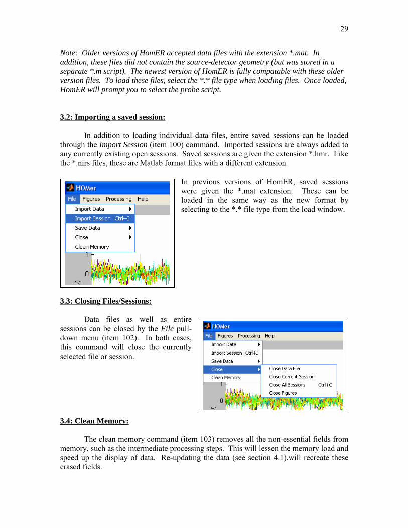
Note: Older versions of HomER accepted data files with the extension *.mat. In addition, these files did not contain the source-detector geometry (but was stored in a separate *.m script). The newest version of HomER is fully compatable with these older version files. To load these files, select the *.* file type when loading files. Once loaded, HomER will prompt you to select the probe script. 3.2: Importing a saved session: In addition to loading individual data files, entire saved sessions can be loaded through the Import Session (item 100) command. Imported sessions are always added to any currently existing open sessions. Saved sessions are given the extension *.hmr. Like the *.nirs files, these are Matlab format files with a different extension.

In previous versions of HomER, saved sessions were given the *.mat extension. These can be loaded in the same way as the new format by selecting to the *.* file type from the load window.

3.3: Closing Files/Sessions: Data files as well as entire sessions can be closed by the File pull-down menu (item 102). In both cases, this command will close the currently selected file or session. 3.4: Clean Memory: The clean memory command (item 103) removes all the non-essential fields from memory, such as the intermediate processing steps. This will lessen the memory load and speed up the display of data. Re-updating the data (see section 4.1),will recreate these erased fields.

30

3.5: Saving Data: Data processed with HomER can be saved for later use. Data can be saved by an individual session (saving only the currently selected session) or by saving all sessions (which saves all open sessions). There are several saving options, which can affect the size of the resulting saved files.

Save minimum: This saves only the most important fields. For example, the end filtered optical density and concentration, as well as the averaged data.

Save in 7.0 format: One of the upgrades from earlier versions to Matlab 7.0 was

a change in the compression of the files and figures. While this made the files more compressed, they no longer worked in older versions of Matlab. By default, HomER will save files such that they maintain backwards compatibility with older Matlab versions, however, this option will save smaller *.hmr files.

31

Chapter 4: Filtering Data The first step in analyzing data within HomER is to filter or update the data. This is a required first step even if no signal processing is desired since updating creates a number of fields that are required for averaging and eventual image reconstruction. Updating the data should always be done as a first step to analysis. Updating consists of a number of calculations including low and high pass filtering of the data, principle component analysis based filtering, and calculation of concentration changes by the Modified Beer-Lambert law. 4.1: Steps involved in updating: Its informative to understand the steps that are taken in updating, since it helps to understand the amount of processing done up to each level of the analysis. For more information, the updating/filtering code is provided in the appendix of this manual.

1. Intensity normalization. The raw intensity data is first normalized to provide a relative (percent) change by dividing by the mean of the data.

The intensity normalized data is then low-pass and/or high pass filtered. After high-pass filtering, unity again added to bring the data back to unity mean.

2. Delta-optical density. The change in optical density is then calculated for each wavelength. This is equal to:

3. Covariance Reduced dOD. Following calculation of delta-optical density, up to two different principle component analysis (PCA) filters are applied to the data. The first PCA filter corrects for motion in the data (i.e. subject head movement). The second PCA filter uses the principle components of the baseline data attempt to project out systemic physiology.

4. delta-Concentration. The covariance reduced dOD data is then

used to calculate delta-concentration from the Modified Beer-Lambert law. This step uses the differential-pathlength and partial volume information set in the advanced filtering options.

( ) ( ) / ONormInten t Inten t Inten=

( ( ))OD Log NormInten tΔ = −

2

2

#1 #1#1 2

#2 #2#2 2

* *[ ] * *[ ]

* *[ ] * *[ ]

Lambda LambdaLambda Hb HbO

Lambda LambdaLambda Hb HbO

OD L Hb L HbO

OD L Hb L HbO

ε ε

ε ε

Δ = +

Δ = +

32

1( ) [ ]T THbX e e e OD−Δ = Δ

5. Covariance reduced dConc. Following the MBLL, a third (potential)

PCA filter is applied to the concentration data (separately for the deoxy and oxy-hemoglobin components).

Note: The display of the data, controlled by the menu (item 10) is listed in order in order of increasing processing (i.e. following the steps just outlined). 4.2: Low/High Pass filtering: Low and high pass filtering of the normalized data is preformed according to the filter cutoffs given by the edit fields (item 3). By default, the filtering step uses the Matlab command filtfilt, which performs

a forward and reverse (zero-phase) iir-filtering. Low-pass and High-pass filtering is done as two separate steps. More information about filtfilt can be found at: (http://www.mathworks.com/access/helpdesk/help/toolbox/signal/filtfilt.html) The default irrfilter design is a 3rd order Butterworth filter. The filter design can be changes in the Advanced Filtering Options menu. (items 62 and 63) More information about these filter designs can be found at the Matlab home-page. Currently, HomER requires that both the Low and High-pass filters have the same design. The filter design can be shown by item 64. This uses the freqz command. (http://www.mathworks.com/access/helpdesk/help/toolbox/filterdesign/freqz.html). 4.3: Motion Correction (PCA filter #1): This is the first of three principle component analyisis (PCA) filtering steps that

are allowed by HomER. The purpose of this step is to attempt to remove the large motion artifacts in the data. This is done by projecting those components (eigen-vectors) that covary between all the source-detector channels. For example, a motion artifact will show as a large change of signal in all source-detector channels. In a PCA analysis, the first (strongest) couple of components calculated from the data will capture most of this motion artifact. Therefore, projecting

33

these first components from the data, will remove these artifacts. The edit field (item 4) sets the number of Singular-vectors that are removed.

There are two modes for this filtering step:

1) If a single value is given in the field (i.e. nSV = 1), then the principle components are calculated from the entire data file (i.e. all wavelengths as one). This is most appropriate for motion correction, since motion of an optode should affect all wavelengths).

2) If two or more values are given (i.e. nSV = [0 1] ), then the principle

components are calculated independently for each wavelength. If more wavelengths are present then values provided, the remaining are assumed to be zero. The PCA filter then acts on each wavelength independently.

Equation: Note on PCA filtering: The prinicple components of a data set do not equate to any one

feature of the data (for example, systemic physiology or motion (etc)). The principle components are simpily a set of basis functions describing the data. PCA filtering attempts to remove features of the data by determining this set of basis functions and then rewriting the data in terms of a limited subset of them. For example, by leaving out the first (strongest) basis function (principle component), the “most dominant features” which covary between all source-detector channels is removed.

Caution should be exercised when using PCA filtering since too much filtering (which may mean any at all) will likely remove components of the desired signal, since the components of the hemodynamic response will not in general be orthogonal to the first nth priniple components of the data. 4.4: Systemic Filtering (PCA filter #2):

1

'[ , , ] ( )

(:,1: ) (1: ,1: ) (:,1: ) '

BaseLine BaseLine

Data

Filtered Data

C dOD dODv s u svd C

EigVects dOD v sdOD dOD EigVects nSV s nSV nSV v nSV

−

==

== −

g

g gg g

34

The second PCA filter uses baseline data to derive the principle components and then projects them from the functional run data. The motivation for this is that the principle components of the baseline data should capture the features of the systemic physiology (blood pressure, respiration, cardiac cycle etc). Projecting these components from the functional run, attempts to filter out these systemic fluctuations from the data. This filter requires multiple values (one for each wavelength) to be entered into item 5. This Filtering step is ONLY available if baseline data is specified. More information about this filter can be found in: Zhang Y. et al. (2005). Eigenvector-based spatial filtering for reduction of physiological interference in diffuse optical imaging. Journal of Biomedical Optics 10(1). 4.5: dConc. Filtering (PCA filter #3): While the last two PCA filters acted on delta-Optical Density, the last PCA filter acts on the concentration of oxy and deoxy-hemoglobin. This allows one to further filter out systemic physisiology (which affects the venous and arterial compartments differently). This filter requires two values (one for oxy and deoxy hemoglobin- in that order) to be entered into item 6. There are two modes for this filter, which are set by item 7

1) Calculate components from data. In this mode, the filter works the same as PCA filter #1, but acts on concentration.

2) Calculate components from baseline

Here, the filter works the same as PCA filter #2. Baseline data must be specified to use the filter in this manner.

4.6: Displaying the SV-spectrum: In deciding to use the PCA filters above, it is important to remove an appropriate number of singular values. Removing too many will compromise the hemodynamic response. The Singular value spectrum can be displayed (Item 9). This will display a window showing the eigen-values for each of the principle components. This represents the “power” in each of the components.

35

4.7: Modified Beer-Lambert Law: Changes in hemoglobin concentrations are related to changes in optical density by the modified Beer-Lambert Law (MBLL). 4.8: Absorption Spectra: There are several choices for the absorption of hemoglobin available. These are

selected in the Advanced Filtering Options menu (item 61). The citation of the currently selected spectrum is given in item 59. The spectrum can be displayed by clicking item 60.

( ) ( )A dpfdOD L lλ μ λ λ= Δ g g

[ ] ( )HbO HbR dpfdOD HbO HbR L lλ λλ ε ε λ= Δ + Δg g g g

1( ' ) * 'HbO

E E E dODHbR

−⎡ ⎤=⎢ ⎥

⎣ ⎦g g

36

All spectra were taken from the Oregon Medical Laser Center (http://omlc.ogi.edu/spectra/)

The full citations for the available spectra are:

1) (Default)

• W. B. Gratzer, Med. Res. Council Labs, Holly Hill, London

• N. Kollias, Wellman Laboratories, Harvard Medical School, Boston

2)

• J.M. Schmitt, "Optical Measurement of Blood Oxygenation by Implantable Telemetry," Technical Report G558-15, Stanford."

• M.K. Moaveni, "A Multiple Scattering Field Theory Applied to Whole Blood," Ph.D. dissertation, Dept. of Electrical Engineering, University of Washington, 1970.

3)

37

• S. Takatani and M. D. Graham, "Theoretical analysis of diffuse reflectance from a two-layer tissue model," IEEE Trans. Biomed. Eng., BME-26, 656--664, (1987).

The option to load a custom spectrum is a feature that is under construction for future releases of HomER.

Multiple wavelengths: When more the two wavelengths are present, concentration is

calculated from the least-squares fit of the hemoglobin spectrum to the data. 4.9: Differential Path-length corrections: A DPF correction can be included in the caluculation of concentration. This will depend on the geometry and subject anatomy (skull thickness etc). This can be specified for all wavelengths together (in which case it is a scaling factor) or individually per wavelength. Note: Unless the option to include the DPF is checked, neither the DPF nor the source-detector distances are taken into account when calculating concentration. This makes the units on concentration, somewhat arbitrary (i.e. Moles * cm / Liter). This is because without the DPF correction, the pathlength is simplily a scaling factor and is inaccurate without this correction… meaning that without DPF correction, one shouldn’t trust the absolute quantity of concentration. Partial-volume Correction: A partial volume correction to the DPF can also be included. This correction only applies to concentration (i.e. no partial volume corrections are ever added to dOD). 4.10: Custom Filtering: This feature is not allowed in the stand-alone version of HomER. In the Matlab 7.0 version, this allows for additional Matlab function calls to be added at the end of the updating step.

38

4.11: Filtering Options: To be written…

4.12: Measurement List Pruning:

Pruning provides a way to remove unwanted source-detector pairs from being included in filtering, averaging and/or imaging (for example noisy or low signal channels). This can be done on the basis of source-detector seperation distances, min/max raw data intensities, or manually by clicking on the SD-geometry (item 2). Removed measurements will appear as dotted lines on the probe. The entire measurement list can be reset by the button above the probe geometry. Removed measurements are NOT included in the PCA analysis. These means that the principle components are calculated from only the remaining (active) measurements. Leaving noisy measurements in will create unwanted

results in the PCA analysis.

39

Chapter 5: Averaging the stimulus response 5.1: Pre-conditioning the stimulus:

The stimulus train is calculated from the “s” variable. To determine the timing of the stimulus, an edge detection can be preformed on this data. This will find the rising edge of each stimulus block. This is designed for dealing with finding the edge of (for example) voltage signals recorded from presentation computer.

Stimulus Threshold- The relative change in signal above which the point is

assumed a stimulus. Tsep- The minimum time seperation between stimuli.

The Reset Stim button recalculates the stimulus train from the “s” variable. The stimulus points are displayed on the data by the Stimulus toggle button. The View Original Stim button will display the original s variable (in blue) on the graph as well. 5.2: User-Defined Stimuli: In addition to supplying the stimulus timing in the s variable with the file, the stimulus timing can be manually entered. Stimuli timing is entered by either listing the times (in seconds) for the start of epoch or (for periodic timing) the stimuli can be specified by:

[Start time: step: Stop time] For example, a stimulus that occurred every 20 seconds, starting at 10 sec for the entire 6 minutes of the run would be specified by:

[10:20:360]

This would put stimulus points at 10,30,50,70… seconds. To specify HomER to use the user-defined stimulus timing, the user-defined stimulus timing field must be filled (item 32) and the toggle button (item 31) must be down.

40

5.3: Removing individual stimulus points. HomER allows you to remove individual stimulus points from the analysis (for example, those points that occurred during a motion artifact etc). This is done by clicking on the green stimulus lines, which turn to red, dotted lines when inactive.

Clicking on the line again will restore the point. The Reset Stim button will restore all stimulus points. 5.4: Removing blocks of data. A second feature that allows stimulus points to be removed from the analysis is to

remove entire blocks of time. This is more appropriate when dealing with deconvolution against the stimulus timing, since the removal of a line would result in the linear regression model considering that epoch as baseline, when in fact it is a noisy activation. Removing blocks of data is done by first RIGHT-clicking on the plot window (item 1). This brings up the context-menu for the window, with a number of other features on it. Chosing to Remove Data, you can select a region of time with a drag-window (click once and then drag the rectangle around the area to remove). This period of time will be highlighted in red. To reset the data, choice the Reset Data feature in the same menu. Choicing not to OverLay TDML (for time-domain measurement list) will make the red area disappear, but the data is still removed. Upon averaging or deconvolution, this data block will be masked out of the analysis. Note: Removing data will have an effect on the efficiency of the deconvolution (stimulus design matrix). This should be used carefully. The features to display the residual (and studentized residuals) should serve to help recognize outliers (artifacts) in the data.

41

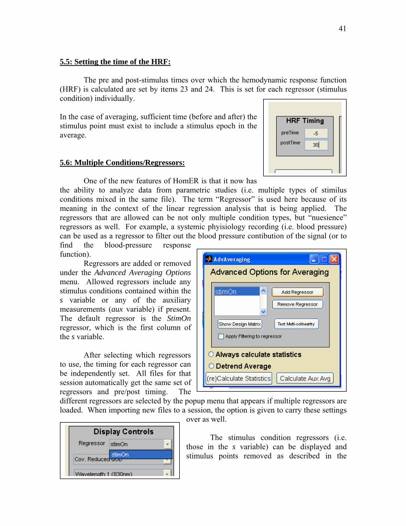
5.5: Setting the time of the HRF: The pre and post-stimulus times over which the hemodynamic response function (HRF) is calculated are set by items 23 and 24. This is set for each regressor (stimulus condition) individually. In the case of averaging, sufficient time (before and after) the stimulus point must exist to include a stimulus epoch in the average. 5.6: Multiple Conditions/Regressors: One of the new features of HomER is that it now has the ability to analyze data from parametric studies (i.e. multiple types of stimilus conditions mixed in the same file). The term “Regressor” is used here because of its meaning in the context of the linear regression analysis that is being applied. The regressors that are allowed can be not only multiple condition types, but “nuesience” regressors as well. For example, a systemic phyisiology recording (i.e. blood pressure) can be used as a regressor to filter out the blood pressure contibution of the signal (or to find the blood-pressure response function). Regressors are added or removed under the Advanced Averaging Options menu. Allowed regressors include any stimulus conditions contained within the s variable or any of the auxiliary measurements (aux variable) if present. The default regressor is the StimOn regressor, which is the first column of the s variable. After selecting which regressors to use, the timing for each regressor can be independently set. All files for that session automatically get the same set of regressors and pre/post timing. The different regressors are selected by the popup menu that appears if multiple regressors are loaded. When importing new files to a session, the option is given to carry these settings

over as well. The stimulus condition regressors (i.e. those in the s variable) can be displayed and stimulus points removed as described in the

42

previous sections. Those from the auxillary variable cannot be pruned. In addition the design matrix (item 87) and the covariance of the design matrix (which tests multi-colinearity of the regressors) (item 86) can be displayed for the choice of regressors. These should be used to judge the efficiency of the design. Equation: Note: Colinearity between regressors can cause the design matrix to be ill-conditioned. This will result in warning messages, but more importantly, will create undesired (and often horribly misleading) results. This can be avoided by carefull planning of the stimulus timing when creating parametric stimulus experiments. 5.7: Averaging: Block averaging of the data can be preformed once the response pre/post timings have been set and the stimulus is in order. Block averaging is preformed by averaging all active data blocks (i.e. those shown as green active stimulus points). Averaging is first preformed within a single run and then averaged across data files. Data files marked as baseline data are ignored (even if they might look to have stimulus points in them). Averaging is also preformed separately between the even and odd stimulus points before being averaged together. This allows the results from the even and odd stimuli to be displayed independently, a feature, which helps identify artifacts that can arise from a single bad data epoch. If multiple regressors (conditions) are selected, HomER averages only those which have binary data (i.e. distinct stimulus points, such as those loaded in the s variable). Regressors such as systemic physiology are ignored (and a warning message is given as such). More detailed information about averaging is found in the appendix to this user’s guide.

i ii

dConc IRF Regressor=∑ g

1_( ' ) '

_Stimulus IRF

X X X ConcPhysiol IRF

−⎡ ⎤= Δ⎢ ⎥

⎣ ⎦g g g

43

Note: The response functions for delta-optical density and delta-concentration are preformed separately. Optical density responses are calculated from the covariance-reduced optical density. Concentration responses are calculated from the covariance-reduced oxy and deoxy-hemoglobin concentrations. These two averages may not be completely consistent with each other, since the cov-reduced concentration data has an additional PCA filtering step. 5.8: Deconvolution: The check box (item 26) determines whether a block averaging or linear regression (deconvolution) is performed. In the case of deconvolution, a linear regression of the data against all of the selected regressors is performed.

There are several good resources on linear regression to which the user is referred for a more detailed description. Linear regression attempts to model the data as a linear superposition of the contribution of all the regressors used. In other words, the contribution from the stimulus (functional response) is the stimulus timing convoluted by the hemodynamic response function (impulse response). Similarly, the contribution from (for example) the cardiac cycle could be modeled as an EKG recording convoluted with a cardiac impulse response function. Linear regression (as used in HomER) attempts to calculate these various impulse response functions. A more detailed description of the linear regression calculations used in HomER are included in the appendix. Note: The use of systemic regressors (such as blood pressure and cardiac cycle) can allow for the calculation of a “cleaner” functional hemodynamic response. This should be used carefully since systemic changes may often be stimulus correlated (i.e. heart rate changes as the subject performs the task). Note: The response functions for delta-optical density and delta-concentration are preformed separately. Optical density responses are calculated from the covariance-reduced optical density. Concentration responses are calculated from the covariance-reduced oxy and deoxy-hemoglobin concentrations. These two averages may not be completely consistent with each other, since the cov-reduced concentration data has an additional PCA filtering step. 5.9: Auxillary Average: HomER also allows for the averaging or deconvolution of the auxillary channels (if present). This is done by item #91 on the Advanced Averaging Menu. This is done exactly the same as with the data.

44

The auxillary averages do NOT automatically update if the averaging conditions change. The average auxillaries button must be pressed each time to reflect the changed parameters.

45

Chapter 6: Image reconstructions Following averaging, image reconstructions can be created for any of the regressor variables (stimulus conditions). Calculation of the forward solutions (i.e. 3pt Green’s functions) and inversion techniques use functions from the PMI Toolbox (also separately available for download at http://www.nmr.mgh.harvard.edu/PMI/). Additional documentation related to these functions is included with this package. Image reconstruction in HomER currently only supports back-projection methods and linear forward models created from semi-infinite (homogeneous) slab geometries. 6.1: Medium Properties: The medium properties, including the absorption and reduced scattering coefficients, as well as the voxel dimensions and reconstruction depth are set by items 48-50 on the imaging tab menu. The absorption and reduced scattering coefficients are defined sepreately for each wavelength. If less values are provided then wavelengths, the remaining wavelengths are assumed to have the properties of the last index. Note: Although the forward matrixes are computed to project changes in optical density, HomER allows image reconstruction of concentration changes using the same forward matrices. In the case of concentration image reconstruction, a spectrally weighted forward matrix is used (the average of all the wavelengths weighted by the extinction coefficients). 6.2: Image Reconstruction: There are three steps to the reconstruction of images:

1. Make Forward Matrix: This function generates the forward models for image reconstruction using the PMI toolbox function genBornMat. This step must be repeated each time the measurement list (see section ??) changes or when switching image types (dOD, concentration, or Contrast/Noise images).

2. Invert Matrix: This function inverts the forward matrix using a back-projection technique. This function uses the inversion technique selected under the Tomography Options menu (see section ??). The default is a back-projection method.

46

3. Make Image: This final command generates and displays the reconstructed image in a new window.

6.3: Image Display: The displayed image is controlled by a number of additional fields on the HomER interface. These control the time range that the image is derived from as well as what type of image is displayed. 6.3.1: Controling the image timing: The image displayed is the average change over a period of time. This timing is controlled by the positioning of the red control bar (item 57) which appears at the bottom of the averaging window. Clicking above this line moves the length of the time range, while clicking below it controls the start time. Note: Item 57 is also used in some of the statistics menus. To move the time range without changing the image timing, toggle the Display Image button to the off position (item 56). Note: Multiple images (with different timings) can be opened at once. This is achieved by clicking the Make Image button again. A new window will appear. The timing and scaling controls now ONLY affect the newest window. 6.3.2: Controling the image scale: Image types: Images are reconstructed for the currently selected regressor. There are three choices for image types:

1. delta-Optical density This will display an image reconstructed from the cov-reduced dOD average response. Each wavelength will be displayed.

2. Contrast-to-noise ratio: This will display an image of the contrast-to-noise ratio of dOD. The noise is taken as either the standard error of the the (cov-reduced) baseline dOD (if baseline is available) or as the standard error of the pre-time (up until the zero-point) for the average response.

3. delta-concentration:

47

This will display images reconstructed from the cov-reduced oxy and deoxy-hemoglobin (with total hemoglobin being the sum of the two). The forward matrices used top generate these images use the spectrally weighted average of the wavelength specific forward models.

6.3.3: Overlaying the probe geometry: The Advanced Imaging Menu provides the option to overlay the probe geometry on each image. 6.4: Movies: Once images are reconstructed, movies of the entire response can be created and saved as AVI files (which can be viewed in most media views or inserted into PowerPoint presentations). All movie commands are found on the processing pull-down menu under imaging.

Make Movie: This command generates the movie from the collection of images. Only one set (i.e. wavelength or hemoglobin species) is generated at a time (all are processed sequentially).

Note: Make Movie uses the Matlab function getframe. Because of this the movie

must be displayed to the screen as it is generated. Do NOT close this window until the movie has been fully created (the window will automatically close).

Play Movie: This command plays the movie in a new window. The Matlab movie function first plays the movie quickly (which is Matlab loading it into memory) and then it plays it again at normal speed.

Save Movie: This command allows you to save a movie once created (movies

do not need to be played before being saved). HomER will prompt for a directory and file name for the *.avi file.

Each wavelength (or concentration) will be saved with the suffix ‘_###nm.avi’ or ‘_HbX.avi’ added to the file name. A separate file is generated for each movie type.

Delete Movie: Movie variables are rather large and tend to really slow the

HomER program when in memory. Deleting movies removes them from the memory.

6.5: Movie Options:

48

The Advanced Imaging Menu allows one to control the display speed and *.avi compression level (type) of the movie file. Tomography Options: This menu allows the user to chose from a selection of inversion techniques. This section of the user’s guide is not yet written

49

Chapter 7: Data display and Export The data processing in HomER is probably just the beginning of the processing needed to turn an experiment into a proper publication, therefore HomER allows several ways to display or export the data so it can be used in other processing. 7.1: Data Export Options:

Saving data fields: By Right-clicking on any of the display windows, the option to save data will be provided. This will allow the user to export the data type that is currently being displayed (i.e. that entire variable) to either a Matlab file (*.mat) or as an ASCII file (which can be read by Excel or other programs). This is done by selecting the save type on the put-file menu (either *.mat or *.dat).

The saved date file will be organized into a column vector for each

measurement. The ml variable refrences each column. This variable is saved along with the data with the *.mat option (but not in ASCII files).

Note: Certain fields are not allowed to be saved as ASCII files. These

include delta-concentration (since it is a three-dimensional array [measurements x time x {HbO2, HbR, HbT} ] and would need to be saved as three separate files) and the SD geometry (right-clicking the probe geometry-item 2).

Copy data: This feature copies the data to the Windows clipboard. This is

done by right-clicking on a displayed data line. Saving session data: Anouther option for exporting the data is to interface

directly with the .hmr format by saving the entire session. This format is described in the appendix to this guide.

7.2: Data Display: Note: Since HomER is being run as a Matlab 7.0 program, all figures saved as .fig files will be compressed in the 7.0 format. This format will not be readable from older Matlab versions (in other words, the figure files will not be able to be re-opened!!!). To get around this problem, when saving figures, one should choice to Save As into a format which will be readable (for example as a tiff or jpeg image). All other data saving (.mat) is done in backward compatible format by default (but I never figured out how to change the menu defaults on the figures in a stand-alone program)

50

There are a number of options for the display of data. Most of these are context specific, meaning that the options available depend on the processing (i.e. whether a block averaging or deconvolution was preformed etc).

Most of these options require no additional explanation. Here, however, are a few

of the finer points to these controls.

7.2.1: Displaying Error-bars: Data that has been block averaged will have error-bars (both standard deviation

and standard error) associated with it. Which of these the error-bars reflect is determined by right-clicking on the average display window and selecting the choice under plot options.

7.2.2: Confidence-bounds:

Data that has been processed by linear regression will have confidence bounds

associated with it. This is accessed by right-clicking on the average display window under plot options. This will over-lay the 95% confidence bounds on the average response.

Note: The option to display confidence bounds is only available AFTER statistics

(see section 8.x) have been calculated on the data and only for the linear regression model.

7.2.3: Residuals:

The residuals of the data that has been processed by linear regression

(deconvolution) can be displayed by right-clicking on the main display window (item 1) and selecting plot residuals under plot options. These will be plotted in a new window. This is only available for cov-reduced dOD or dConc.

Note: The option to display residuals is only available AFTER statistics (see

section 8.x) have been calculated on the data and only for the linear regression model.

7.2.4 Model Fit:

The modeled response of the data that has been processed by linear regression

(deconvolution) can be displayed by right-clicking on the main display window (item 1) and selecting plot model under plot options. The model is the regressor data convoluted by the impulse response function(s). (i.e. Data – Model = Residuals). The model is plotted as dotted lines over the cov-reduced dOD or dConc. data

51

Note: The option to display model is only available AFTER statistics (see chapter 8) have been calculated on the data and only for the linear regression model.

7.3: Plot in new window

All display windows can be replotted in new windows by right-clicking on the original display and selecting New Figure.

7.4: Plot All:

The command to Plot All (item 108) will open a new window and plot the average response for each (active) source-detector pair as they are spatially distributed. This will plot the data as either dOD or dConc according to the display controls. Although this feature works well for simple probe geometries, complex or overlapping probes may not be displayed properly with this option.

7.5: Plot PSD:

This will display the power-spectrum density (i.e. Fourier Transform) of the data. This will not be available for concentration data.

7.6: Display All:

This option will display the data as a psuedo-colored image of <measurement channel> verses <time>. The measurement channels are referenced by the ml variable.

52

Chapter 8: Statistical Analysis

HomER can perform a number of statistical tests on the data, which can help determine the proper way to process the data. These use many functions from the Matlab Statistics toolbox. These are built into the stand-alone version, but are required for the full function of the code under Matlab.

8.1 Processing Statistics: Statistics are calculated by the (Re)Calculate Statistics command (item 90) on the Advanced Averaging Menu. This command will perform an ANOVA analysis for the model fit on the entire time course. This also performs an effects analysis on the functional responses. If the Display Avg. All toggle button is down (i.e. the session average is being displayed), then the Calculate Statistics button will calculate the statistics for the session average. If this button is up, then only the currently displayed data file is processed. ANOVA analysis: An analysis of variance (ANOVA) analysis is preformed on the model fit This section of the user’s guide is not yet written

53

Chapter 9: Region-of-interest Analysis

This section of the user’s guide is not yet written

54

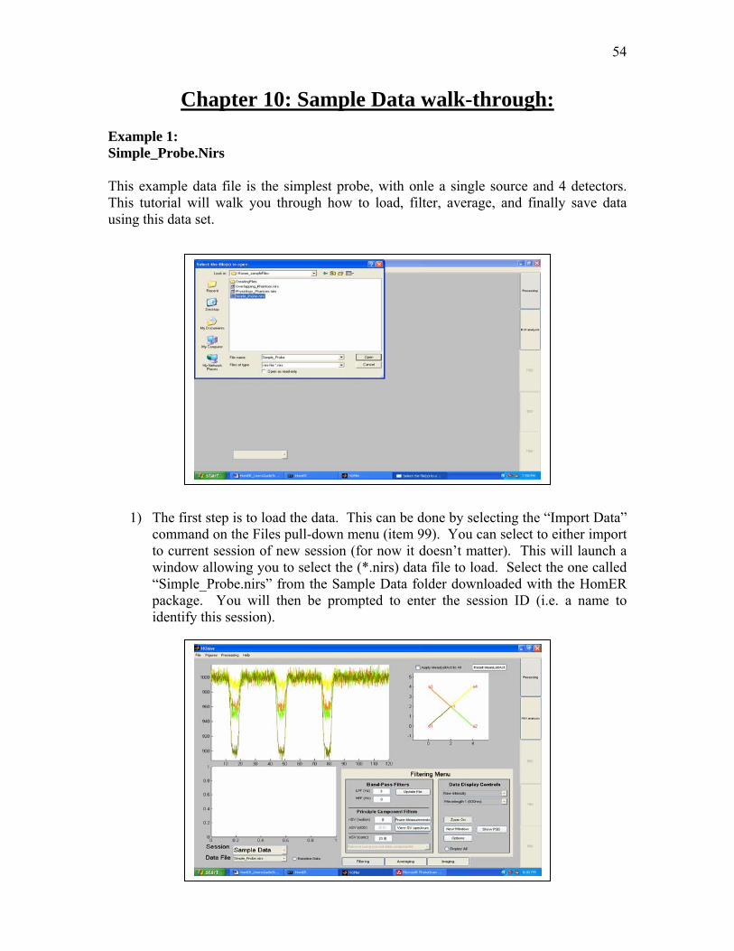
Chapter 10: Sample Data walk-through: Example 1: Simple_Probe.Nirs This example data file is the simplest probe, with onle a single source and 4 detectors. This tutorial will walk you through how to load, filter, average, and finally save data using this data set.

1) The first step is to load the data. This can be done by selecting the “Import Data”

command on the Files pull-down menu (item 99). You can select to either import to current session of new session (for now it doesn’t matter). This will launch a window allowing you to select the (*.nirs) data file to load. Select the one called “Simple_Probe.nirs” from the Sample Data folder downloaded with the HomER package. You will then be prompted to enter the session ID (i.e. a name to identify this session).

55

2) After selecting the file, HomER should appear as shown to the left. The probe geometry is shown in window 2. Clicking on this window will select different source-detectors to display. You can select which wavelength is displayed by item 11. There are 2 wavelengths in this file. Only “Raw Data” is avalaible until the data has been updated.

3) The next step is to UPDATE the data. First, enter the filter parameters into the

edit fields (item 3). The first field sets the low-pass filter (LPF) and the second sets the high-pass filter (HPF). To ignore one or both of these filters, the fields can be entered as “[]” (empty set). Once one of these fields has changed, HomER will make visible the “Update buttons”. Click here to update the files. This will apply the filter settings and (since this is the first time through), this will create the delta-optical density (etc) fields.

4) Once updated, you can now change the view to display processed data traces (as shown to the left). Concentration data is additionally displayed by the Figures>>Display Options>>Concentrations pull-down menu. This lets you select to display HbO2, HbR, or total-Hb species.

You can display the data in a new window by right-clicking with the mouse on the window. The data can also be copied to the clipboard by right-clicking on a data line. Data can also be exported to file (either ASCII or Matlab) in this way as well. The choices for displaying data are given in order of increasing processing (for example, raw data is the least processed, while Covarience reduced dConcentration has the most filtering/processing applied to it).

56

5) You can now calculate the average response. Switch to the averaging menu by selecting the averaging tab on the bottom of the screen. This will bring up options for displaying the stimulus.

To display the stimulus, click on the toggle-button called “Show Stim”. This will plot green lines showing the start of each epoch. This was taken from the “s” variable that is part of the nirs file structure. This variable may need to be manually pruned slightly to make it correct (for example, if the s variable was recorded from a stimulus computer and may need edge detection applied to it to determine the start times). The Stim Thresh variable controls the minimum amplitude of an edge (in normalized units of the derivative of the s-variable). The Stim Tsep sets the minimum time seperation between stim events. Reset Stim (available after one of these fields has changed) applies the changes and replots the epochs. Stimulus epochs can be removed by mouse clicking on the green lines. This will change the line color to red, indicating that the epoch is inactive. This can be used to manually remove epochs that have too much noise (i.e. motion artifacts).

57

The timing for the response is set by the PreTime and PostTime fields. This is the time before and after the stimulus start (green line) to calculate the response. Once the stimulus has been satisfactorally modified, you can click the button called “Calculate Average”. This will perform a block average of the epochs. In the case shown the the left, since the last stimulus was removed (i.e. a red line), the average is calculated from only the first two epochs. The response is now plotted in window 3.

6) You can now add statistics to the response. First open the Advanced Averaging Options menu. Now click the “Calculate Statistics” button. (The option to always calculate stats is given above this… this will automatically perform this analysis everytime the average button is clicked, but this can become computationally expensive for larger data sets).

58

Once the statsistics have been calculated, you can view them by using the mouse to right-click on the red bar on the plot window. This red bar selects the contrast timing for the statistics (also for image reconstruction). This will bring up a menu with information about the effects analysis of the hemodynamic model. If you right-click on a data trace in the window, you can display the ANOVA information about the individual source-detector data. Lastly, we can save our analysis for loading again in the future. This is done under the pull-down menu FILES>>Save Data. In this case, (since we only have a single session) we want to save session. This will bring up the window prompting us to select a file name and directory. Saved data will be given the extension *.hmr. If we had multiple sessions open, “save all sessions” saves everything, while “save current session” only save the currently selected session.

59

Example 2: Image Reconstruction This next example uses the OverLapping_Probe.nirs sample data file to demonstrate some of HomER’s image reconstruction features.

1) First, load the sample file named “OverLapping_Probe.nirs” following the steps outlined in the previous example.

2) Filter

(Update) and average the data as done in example 1. The result should be similar to the figure below. Once the data has been averaged, we can now reconstruct images. This sample data has overlapping measurements, which allows us to perform tomographic reconstructions (rather then simple back-projections)

3) Go to the Imaging window by clicking on the imaging tab on the lower right.

You can specify the dimensions of the reconstructed image as well as the absorption/scattering coeffiecients for each wavelength. The default depth for the image is 1cm deep.

60

4) Make the forward matrix by clicking the “Make Matrix” button.

5) Invert this matrix using the “Invert” button. Since we haven’t changed any of the

settings yet, this will use the default, which is to perform a back-projection of the data.

6) Click “Make Image” to make the final image. A new window should pop-up with

the dOD images in it. These images are the average HRF contrast over the time window defined by the red bar in window 3. Clicking on this bar (and dragging it) will move the contrast window and update the image.

You can change the scaling of the image by manually changing the Max/Min edit fields (type 999 to use autoscaling).

7) You can change the appearance of the images by clicking the button called “Display options”. This will bring up a new window as shown to the left. The check boxes for showing probe on image or colorbar will add these to the image as shown. The images may need to be redisplayed (i.e. click display image or the red bar) before these changes take effect

8) We can also perform tomographic reconstructions of images. To demonstrate this, first change the data type from dOD to dConc (item 53). Now, click the button marked “DOT options”. It will pop-up a new window as shown to the left.

61

Since we are now reconstructing dConc, we will be using spectral priors in the image reconstruction (i.e. see: Li et al. 2004. Optics Letters 29(3): 256-259). You can adjust the regularization amount through the “a” edit field and also the type of noise term that is used. This probe will still require quite a bit of regularization. The “Make Image” button applies these settings (this is the same as the “Make Image” button on the main page). 9) We will now reconstruct a movie of the activation and export it to a avi file so

that we can use it later. First select Processing >> Imaging >> Movies from the top pull-down menu. Now, chose the function to make movie. This will start forming the movie in a new window. This function uses the matlab function getframe, which means that it must plot each image before adding it to the movie. During this process, DO NOT close the window (this could result in an error). The window will automatically close when finished.

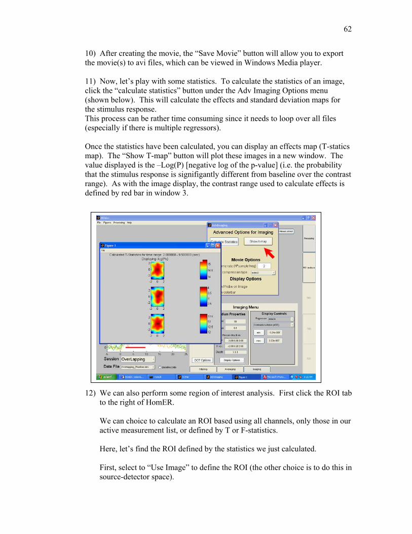
62

10) After creating the movie, the “Save Movie” button will allow you to export the movie(s) to avi files, which can be viewed in Windows Media player.

11) Now, let’s play with some statistics. To calculate the statistics of an image, click the “calculate statistics” button under the Adv Imaging Options menu (shown below). This will calculate the effects and standard deviation maps for the stimulus response. This process can be rather time consuming since it needs to loop over all files (especially if there is multiple regressors). Once the statistics have been calculated, you can display an effects map (T-statics map). The “Show T-map” button will plot these images in a new window. The value displayed is the –Log(P) [negative log of the p-value] (i.e. the probability that the stimulus response is signifigantly different from baseline over the contrast range). As with the image display, the contrast range used to calculate effects is defined by red bar in window 3.

12) We can also perform some region of interest analysis. First click the ROI tab to the right of HomER. We can choice to calculate an ROI based using all channels, only those in our active measurement list, or defined by T or F-statistics. Here, let’s find the ROI defined by the statistics we just calculated. First, select to “Use Image” to define the ROI (the other choice is to do this in source-detector space).

63

Clicking the button “Define Threshhold” will open a window with the image. The slider bar to the right is used to set the thresh-hold. Pixels included in the ROI will be shown in red (see below).

We have now defined the ROI, to calculate the average, first select whether you want this ROI calculated from the first, second, or union of wavelengths (union means the pixel must be active in all wavelengths to be included).

Since we want to use the statistics to define the ROI, we must also select

the “Use statistical ROI” option. Click the calculate ROI button.

The ROI time course will now be shown in the window.

64

13) Under the Figures pull-down menu at the top of HomER, the option to Plot All will display an image of the probe showing the time-course for each source detector pair. This is displayed as dOD or dConc (Red-HbO2; Blue-rHb; Green- total-Hb).

65

Example 3: Multiple Regression. This section has yet to be written…

66

67

68

69

Appendix I: HomER data format This section describes the format of the HomER variable (DOT). The DOT variable is a structured cell array. Each session is indexed to a cell in this array. For example, DOT{1} returns the fields for the first session (cells are indexed with curly {} brackets). Session Fields: DOT.subjectNum ------------ Session (Subject) Name DOT.SDGfilenm ------------ Source-Detector file Name DOT.SDGpathnm ------------ Path to Source-Detector file DOT.SD ------------ Source-Detector Variable DOT.SD.Lambda ------------ Wavelength List DOT.SD.SrcPos ------------ Source Positions DOT.SD.SrcAmp ------------ Source Amplitude (Gains) DOT.SD.DetPos ------------ Detector Positions DOT.SD.DetAmp ------------ Detector Amplitudes (Gains) DOT.SD.nSrcs ------------ Number of Sources DOT.SD.nDets ------------ Number of Detectors SD.color ------------ Colors used in displays SD.currentFile ------------ Index to currently selected file SD.plotLst ------------ Indices to currently plotted data SD.SrcPicked ------------ Source position currently picked SD.ImgAvgStart ------------ Start timing for contrast timing SD.ImgAvgLen ------------ Length of timing for contrast SD.data ------------ Data file structure- see below SD.dataAvg ------------Averaged file structure- see below SD.img ------------ Recon Image structure- see below SD.roi ------------ ROI structure- see below SD.roiAvg ------------ ROI (multi-session)- see below

70

Data Fields: The data (raw through processed) for each data file within a session is contained within the DOT.data(file) variable. This is a structured arrary, indexed by the file number. %File descriptors DOT.data.FILEpathnm ------------ Path to the file DOT.data.filenm ------------ Name of the data file DOT.data.BaselineData ------------ {Flag} – is file baseline data % Filtering parameters DOT.data.lpf ------------ Low pass filter value DOT.data.nSV ------------ # of SV to remove by PCA #1 DOT.data.hpf ------------ High pass filter value DOT.data.nSV_dOD ------------ # of SV to remove by PCA #2 DOT.data.nSV_dConc ------------ # of SV to remove by PCA #3 DOT.data.dOD_UpToDate ------------ {Flag} – is filtered? DOT.data.avgUpToDate ------------ {Flag} – is averaged? % Data fields DOT.data.MeasList ------------The ml variable DOT.data.MeasListAct ------------ Active measurements (binary) DOT.data.nMeas ------------Number of Measurements DOT.data.Sact DOT.data.Dact DOT.data.raw ------------The orignal (d variable) data DOT.data.norm ------------Intensity Normalized, LPF DOT.data.norm_cov ------------Cov Reduced (PCA #1) DOT.data. Intens_hpf ------------The high-pass filter correction DOT.data.dOD ------------delta-optical density DOT.data.dODc ------------Cov-reduced dOD (PCA #2) DOT.data.dConc ------------delta-concentration DOT.data.dConcc ------------ Cov-reduced dConc (PCA #3) DOT.data.t ------------ The time (t) variable DOT.data.svs ------------ Single-value spectrum (PCA #1) DOT.data.svsConc ------------ Single-value spectrum (PCA #3) DOT.data.Aux ------------The auxillary data

71

% Data Averaged fields DOT.data.HRF ------------Hemodynamic response-see below DOT.data.AuxAvg ------------Auxillary response-see below DOT.data.TDML ------------Block removal matrix DataAvg Fields: DOT.dataAvg.MeasList ------------The ml variable for combined files DOT.dataAvg.MeasListAct ------------ Active measurements (binary) DOT.dataAvg.HRF ------------Hemodynamic response-see below DOT.dataAvg.HRF_stats ------------Response statistics-see below HRF Fields: The hemodynamic response variable (under either DOT.data.HRF, DOT.DataAvg.HRF, DOT.ROI.HRF, or DOT.ROIavg.HRF) describes the averaged data from the individual file, average of all files in a session, region-of-interest average within a session, or region-of-interest average between sessions. This structure is indexed by regressor (i.e. HRF(1) first regressor). DOT.[].HRF.type ------------Regressor name DOT.[].HRF.regdata ------------Regressor data variable DOT.[].HRF.StimOn ------------Stimulus variable (if binary) DOT.[].HRF.numStim ------------Number of epochs (if app) DOT.[].HRF.pretime ------------Pretime of impulse response DOT.[].HRF.posttime ------------Posttime of impulse response DOT.[].HRF.lpf ------------Low-pass value (if used) DOT.[].HRF.hpf ------------High-pass value (if used) DOT.[].HRF.UseFilter ------------Flag- pre-filter regressor? Response data: DOT.[].HRF.tHRF ------------Response timing DOT.[].HRF.nHRF ------------Number of degrees of freedom DOT.[].HRF.Avg ------------dOD (covariance reduced) average DOT.[].HRF.AvgC ------------dConcentraion average DOT.[].HRF.AvgOdd ------------dOD (odd epochs only) DOT.[].HRF.AvgEven ------------dOD (even epochs only)

72

DOT.[].HRF.AvgStdErr ------------Standard Error dOD DOT.[].HRF.AvgStd ------------Standard Deviation dOD DOT.[].HRF.AvgCStdErr ------------Standard Error dConcentration DOT.[].HRF.AvgCStd ------------Standard Dev. dConcentration HRF statistics (regressor specific): DOT.[].HRF.to ------------dOD T-statistics DOT.[].HRF.P ------------dOD T-statistics (p-value) DOT.[].HRF.Conf_High ------------dOD 90% upper bound DOT.[].HRF.Conf_Low ------------dOD 90% lower bound HRF_Stats Fields (ANOVA): DOT.dataAvg.HRF_Stats.Fo ------------Model F-Statistic DOT.dataAvg.HRF_Stats.P ------------Model F-Statistic (p-value) DOT.dataAvg.HRF_Stats.StdRes ------------Studentized residual DOT.dataAvg.HRF_Stats.PRESS ------------PRESS statistic DOT.dataAvg.HRF_Stats.R2Adj ------------R^2 (adjusted) statistic Img Fields: DOT.IMG.A ------------Forward Model DOT.IMG.Ainv ------------Inverse Model DOT.IMG.Medium ------------Forward Model Medium DOT.IMG.Medium.idxRefr ------------Index of refraction DOT.IMG.Medium.Muao ------------Absorption coefficient DOT.IMG.Medium.Muso ------------Reduced Scattering coefffienct DOT.IMG.Medium.g ------------Anisotopic factor DOT.IMG.Medium.Geometry ------------Semi infinite DOT.IMG.Medium.Slab_Thickness ------------Slab thickness (cm) DOT.IMG.Medium.CompVol DOT.IMG.Medium.CompVol .Type ------------“Homogenous” DOT.IMG.Medium.CompVol .X ------------X coordinates (cm) DOT.IMG.Medium.CompVol Xstep DOT.IMG.Medium.CompVol Y ------------Y coordinates (cm) DOT.IMG.Medium.CompVol Ystep DOT.IMG.Medium.CompVol Z ------------Z coordinates (cm) DOT.IMG.Medium.CompVol ZStep DOT.IMG.img ------------Reconstructed Image

73

DOT.IMG.tHRF ------------Image response timing DOT.IMG.Movie ------------Stored Movie

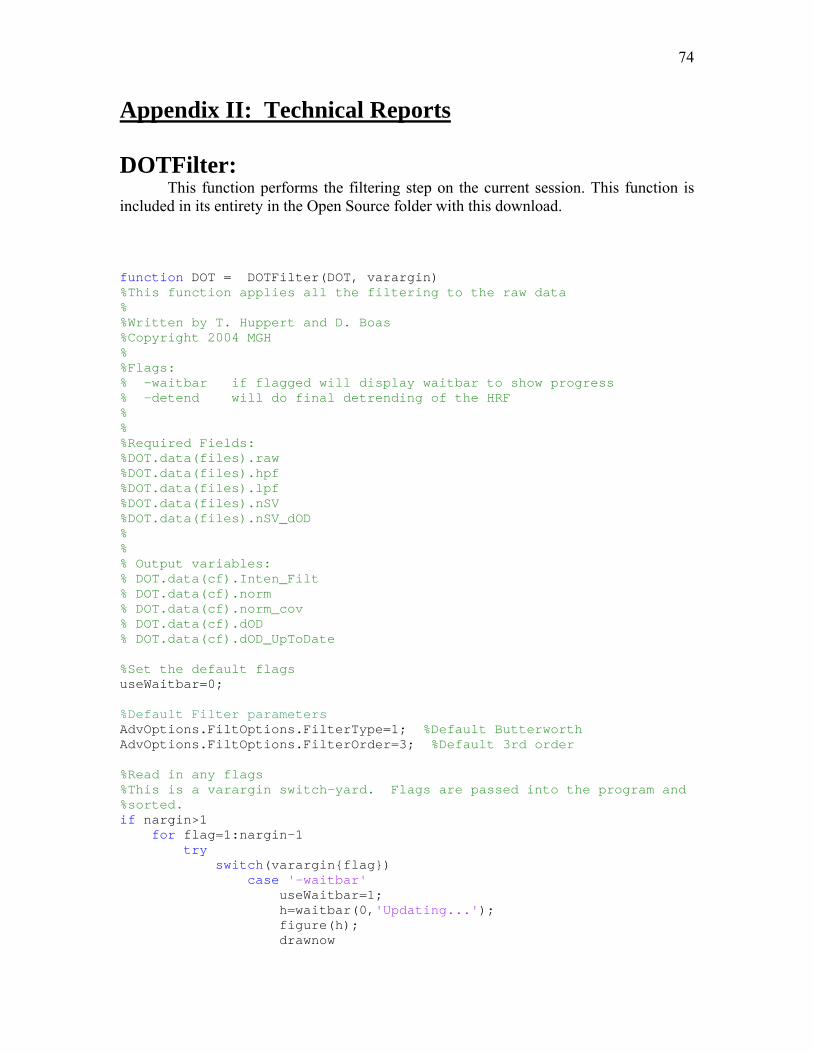
74

Appendix II: Technical Reports DOTFilter:

This function performs the filtering step on the current session. This function is included in its entirety in the Open Source folder with this download. function DOT = DOTFilter(DOT, varargin) %This function applies all the filtering to the raw data % %Written by T. Huppert and D. Boas %Copyright 2004 MGH % %Flags: % -waitbar if flagged will display waitbar to show progress % -detend will do final detrending of the HRF % % %Required Fields: %DOT.data(files).raw %DOT.data(files).hpf %DOT.data(files).lpf %DOT.data(files).nSV %DOT.data(files).nSV_dOD % % % Output variables: % DOT.data(cf).Inten_Filt % DOT.data(cf).norm % DOT.data(cf).norm_cov % DOT.data(cf).dOD % DOT.data(cf).dOD_UpToDate %Set the default flags useWaitbar=0; %Default Filter parameters AdvOptions.FiltOptions.FilterType=1; %Default Butterworth AdvOptions.FiltOptions.FilterOrder=3; %Default 3rd order %Read in any flags %This is a varargin switch-yard. Flags are passed into the program and %sorted. if nargin>1 for flag=1:nargin-1 try switch(varargin{flag}) case '-waitbar' useWaitbar=1; h=waitbar(0,'Updating...'); figure(h); drawnow

75

case '-AdvOptions' AdvOptions=varargin{flag+1}; end end end end %%%%%%%%%%%%%%%%%%%%%%%%%%%%%%%%%%%%%%%%%%%%%%%%%%%%%%%%%%%%% cf = DOT.currentFile; %Grab the current file being used in this

session Intens = DOT.data(cf).raw; %set d1 to the raw data then find the mean of the raw data fs = 1/(DOT.data(cf).t(2)-DOT.data(cf).t(1)); % sampling frequency [timepts,measurements]=size(Intens); lpf = DOT.data(cf).lpf; %Hz, low pass frequency hpf = DOT.data(cf).hpf; %high pass frequency %do the LPF Note: The MakeFilter program takes in the filter type {1= Butterworth, 2= Chebyshev type I, 3= Chebyshev type II, 4 = Elipic} and the Filter parameters {cut-off freq, sample freq, high/low, stop-band, ripple} and outputs the correct filter paraters (for example [fb,fa] =butter(order,[wn]*2/fs) ); %This section of code returns the filter parameters and then applies them using filtfilt to the Intens variable. The new variable Intens_LPF is now low-pass filtered. if lpf>0 & lpf<fs/2; if AdvOptions.FiltOptions.FilterType==1 [fb,fa] = MakeFilter(AdvOptions.FiltOptions.FilterType,…

AdvOptions.FiltOptions.FilterOrder,fs,lpf,'low'); elseif AdvOptions.FiltOptions.FilterType==4 [fb,fa] = MakeFilter(AdvOptions.FiltOptions.FilterType,…

AdvOptions.FiltOptions.FilterOrder,fs,lpf,'low',… AdvOptions.FiltOptions.Filter_Rp,… AdvOptions.FiltOptions.Filter_Rs);

else [fb,fa] = MakeFilter(AdvOptions.FiltOptions.FilterType,…

AdvOptions.FiltOptions.FilterOrder,fs,lpf,'low',… AdvOptions.FiltOptions.Filter_Rp);

end %[fa,fb]=butter(FilterOrder,lpf*2/fs); Intens_LPF=filtfilt(fb,fa,Intens); else if lpf>fs/2;

h=warndlg('Low pass filter frequency exceeds Nyquist frequency');

figure(h);

76

uiwait(h); end %do nothing (If didn’t LPF, then Intens_LPF is the same as Intens) Intens_LPF=Intens; end %Update the Waitbar (if usewaitbar flag was active) if useWaitbar h=waitbar(1/3,h); figure(h); end %Normalize data and convert to dOD meanIntens = mean(abs(Intens_LPF),1); %Take abs() to change from I/Q to reals Intens_Norm = abs(Intens_LPF./(ones(timepts,1)*meanIntens)); %set dm1 to the normalized data list The variable Intens_Norm (processed up untill this point) is the one displayed to the screen when the choice of Normalized Intensity is selected %Do the motion correction PCA filter (PCA filter #1) nSV = DOT.data(cf).nSV; %Number of Singular vectors to remove Intens_Norm_zM=Intens_Norm -1; %zero mean the data if length(nSV)<2

%If only one value was provided then preform the PCA analysis on both wavelengths together…

lst=find(DOT.data(cf).MeasListAct); %The active measuyrements

only c = Intens_Norm_zM(:,lst).' * Intens_Norm_zM(:,lst); %covarience matrix [v,s,foo] = svd(c); %single value decomposition and store as v,s,foo DOT.data(cf).svs = diag(s); %Store the variable for display by

SV-Spectrum if nSV>0 %If the nSV is a valid number, the perform the PCA filter u = Intens_Norm_zM(:,lst)*v*inv(s); lstSV = 1:nSV; Norm_Cov = Intens_Norm_zM;

Norm_Cov(:,lst) = Intens_Norm_zM(:,lst) - u(:,lstSV)*s(lstSV,lstSV)*v(:,lstSV)';

else Norm_Cov = Intens_Norm_zM;

77

end else %This is the case when more then one value was provided. Do the PCA per wavelength. This means we loop over the number of wavelengths

Norm_Cov = Intens_Norm_zM; %So those measurements which don’t get updated (i.e. not on the active ML) carry through

%If the number of values provided is less then the number of wavelengths, then zero-fill the rest

if length(nSV)<length(DOT.SD.Lambda) nSV(end:length(DOT.SD.Lambda))=0; end DOT.data(cf).svs=[]; %Loop over the number of wavelengths for idxLambda=1:length(DOT.SD.Lambda) if size(DOT.data(cf).MeasListAct,1)<

size(DOT.data(cf).MeasListAct,2)

DOT.data(cf).MeasListAct=DOT.data(cf).MeasListAct'; end

lst=find(DOT.data(cf).MeasList(:,4)==idxLambda &… DOT.data(cf).MeasListAct); %lst if the list of measurements at THIS wavelength and on the active ML

c = Intens_Norm_zM(:,lst).' * Intens_Norm_zM(:,lst); %covarience matrix [v,s,foo] = svd(c); %single value decomposition and

store as v,s,foo

DOT.data(cf).svs(:,idxLambda) = diag(s); if nSV(idxLambda)>0 u = Intens_Norm_zM(:,lst)*v*inv(s); lstSV = 1:nSV(idxLambda);

Norm_Cov(:,lst) = Intens_Norm_zM(:,lst) - u(:,lstSV)*s(lstSV,lstSV)*v(:,lstSV)';

end end end Norm_Cov=Norm_Cov+1; %add one to undo the effect of zero-mean %do the HPF %This is the same basic process as the LPF if hpf>0 & hpf<fs/2;

78

if AdvOptions.FiltOptions.FilterType==1 [fb,fa] = MakeFilter(AdvOptions.FiltOptions.FilterType,…

AdvOptions.FiltOptions.FilterOrder,fs,hpf,'high'); elseif AdvOptions.FiltOptions.FilterType==4 [fb,fa] = MakeFilter(AdvOptions.FiltOptions.FilterType,…

AdvOptions.FiltOptions.FilterOrder,fs,hpf,'high',… AdvOptions.FiltOptions.Filter_Rp,… AdvOptions.FiltOptions.Filter_Rs);

else [fb,fa] = MakeFilter(AdvOptions.FiltOptions.FilterType,…

AdvOptions.FiltOptions.FilterOrder,fs,hpf,'high',… AdvOptions.FiltOptions.Filter_Rp);

end %[fa,fb]=butter(FilterOrder,hpf*2/fs); Norm_Cov_HPF =filtfilt(fb,fa,Norm_Cov)+1; else if hpf>fs/2; h=warndlg('High pass filter frequency exceeds Nyquist frequency'); figure(h); uiwait(h); end %do nothing Norm_Cov_HPF =Norm_Cov; end dOD_Norm = -log(Norm_Cov_HPF); %delta-Optical Density is the negative

log of the normalized data The variable dOD_Norm (processed up untill this point) is the one displayed to the screen when the choice of dOD is selected if useWaitbar h=waitbar(2/3,h); figure(h); end %Put the variables into the DOT format. DOT.data(cf).Intens_hpf = abs(Intens_HPF); DOT.data(cf).norm = abs(Intens_Norm); DOT.data(cf).norm_cov = abs(Norm_Cov); DOT.data(cf).dOD = abs(dOD_Norm).*sign(real(dOD_Norm));

79

if useWaitbar h=waitbar(3/3,h); figure(h); end DOT.data(cf).dOD_UpToDate = 1; if useWaitbar close(h); end return … The output of this function is the Optical Density variable (and all processing done up until then). The second and third PCA filters and the MBLL are handled by a second program.

80

HomERFilt: %This is the partial code from the filtering script. Each data file (for the current session) is sequentially passed through this function. %This first part, just makes the call to the DOTFilter program (see above) passing it the correct flags (etc). AdvOptions=get(handles.OptionsStore,'userdata'); if DOT{currentsub}.data(cf).dOD_UpToDate dd1 = DOT{currentsub}.data(cf).dOD; waitbarcount=waitbarcount+3; else

if isfield(AdvOptions,'FiltOptions') & isfield(AdvOptions.FiltOptions,'FilterType') DOT{currentsub} = DOTFilter(DOT{currentsub},'-AdvOptions',AdvOptions);

else DOT{currentsub} = DOTFilter(DOT{currentsub}); end end %This performs the second (dOD-with Baseline) PCA filtering step (see later description) DOT{currentsub}=PCAFilter(DOT{currentsub}); %This is now the cov-reduced dOD variable dd1c = DOT{currentsub}.data(cf).dODc; The variable dd1c (processed up untill this point) is the one displayed to the screen when the choice of dOD-cov.reduced is selected %Now we start applying the MBLL law. We first do the partial volume/DPF corrections (if indicated to do so by the Adv. Averaging Window) %Do partial volume/pathlength correction if desired if isfield(AdvOptions, 'FiltOptions') &…

AdvOptions.FiltOptions.UsePartialVolumeCorr==1 partialVolCorr=AdvOptions.FiltOptions.PartialVolumeCorr; else %Dummy settings partialVolCorr=ones(length(DOT{currentsub}.SD.Lambda),1); end if isfield(AdvOptions, 'FiltOptions') & …

AdvOptions.FiltOptions.UsePathLengthCorr==1

81

DPF=AdvOptions.FiltOptions.DPF; MeasList=DOT{currentsub}.data(cf).MeasList; Distances=((DOT{currentsub}.SD.SrcPos(MeasList(:,1),1)-

DOT{currentsub}.SD.DetPos(MeasList(:,2),1)).^2 +... (DOT{currentsub}.SD.SrcPos(MeasList(:,1),2)-DOT{currentsub}.SD.DetPos(MeasList(:,2),2)).^2 +... (DOT{currentsub}.SD.SrcPos(MeasList(:,1),3)-DOT{currentsub}.SD.DetPos(MeasList(:,2),3)).^2).^0.5;

else %Dummy settings

DPF=ones(nLambda,1); Distances=ones(size(DOT{currentsub}.data(cf).MeasList,1),1); end %Apply the corrections to the dOD variable (now has units of cm-1) for idx=1:nLambda lst= find(DOT{currentsub}.data(cf).MeasList(:,4)==idx); for idx2=1:length(lst)

dd1c(:,lst(idx2))=dd1c(:,lst(idx2))*partialVolCorr(idx)/… (DPF(idx)*Distances(lst(idx2)));

end end %Update the progress bar waitbarcount=waitbarcount+1; try updateWaitbar=waitbar(waitbarcount/waitbartotal,updateWaitbar,msg); catch updateWaitbar=waitbar(waitbarcount/waitbartotal,msg); end figure(updateWaitbar); %Now we convert to concentrations. The GetExtinctions function returns the extinction coefficients for the specified wavelengths. It uses a look-up table (roughly every 1-5nm depending on spectra source) and uses a linear interp to determine intermediate wavelengths (so any wavelength can be used) %GetExtinctions(Wavelengths, AbsSprectum Type). AbsSprectum Type = 1 (Default/ if type not provided)

• W. B. Gratzer, Med. Res. Council Labs, Holly Hill, London

• N. Kollias, Wellman Laboratories, Harvard Medical School, Boston

AbsSprectum Type = 2

• J.M. Schmitt, "Optical Measurement of Blood Oxygenation by Implantable Telemetry," Technical Report G558-15, Stanford."

82

• M.K. Moaveni, "A Multiple Scattering Field Theory Applied to Whole Blood," Ph.D. dissertation, Dept. of Electrical Engineering, University of Washington, 1970.

AbsSprectum Type = 3

• S. Takatani and M. D. Graham, "Theoretical analysis of diffuse reflectance from a two-layer tissue model," IEEE Trans. Biomed. Eng., BME-26, 656--664, (1987).

%convert to concentrations if ~isfield(AdvOptions,'FiltOptions') | ~isfield(AdvOptions.FiltOptions,'AbsSpect') AdvOptions.FiltOptions.AbsSpect=1; end e = GetExtinctions(…

DOT{currentsub}.SD.Lambda,AdvOptions.FiltOptions.AbsSpect); e = e(:,[1 2]); einv = inv( e'*e )*e'; %For Least-squares solution ml = DOT{currentsub}.data(cf).MeasList; lst = find( ml(:,4)==1 ); for idx=1:length(lst) ML_lst=find(ml(:,1)==ml(lst(idx),1) & ml(:,2)==ml(lst(idx),2)); SD_lst=ml(ML_lst,:); [foo, ord]=sort(SD_lst(:,4)); concs(:,:,idx) = ( einv * dd1c(:,ML_lst(ord))' )'; end concs(:,3,:)=concs(:,1,:)+concs(:,2,:); %add total Hb =Oxy + deOxy concetration- stores to tensor of D x 3 x Ml concs = permute( concs, [1 3 2]); %Update the progress bar waitbarcount=waitbarcount+1; updateWaitbar=waitbar(waitbarcount/waitbartotal,updateWaitbar,msg); figure(updateWaitbar); DOT{currentsub}.data(cf).dConc = concs; The variable concs (processed up untill this point) is the one displayed to the screen when the choice of delta-Concentration is selected

83

%The final step is to apply the PCA filter (#3) on the dConc data. See later description. if get(handles.HomER_PCA_conc,'value')==2 UseBaselinePCA=1; else UseBaselinePCA=0; end %dConc PCA filtering step DOT{currentsub}=PCAFilterConc(DOT{currentsub},UseBaselinePCA); %The rest of this code deals with updating the displays to HomER etc…

84

PCAFilter: function DOT=PCAFilter(DOT) %This function applies the PCA filter based on the components of the %baseline % %Required Inputs: %DOT.SD.Lambda %DOT.data(cf).BaselineData %DOT.data(cf).dOD %DOT.data(cf).MeasList %covariance of dOD on each wavelength <moved outside if/end block so it is always preformed cf = DOT.currentFile; nLambda = length(DOT.SD.Lambda); if DOT.data(cf).BaselineData mlAct=DOT.data(cf).MeasListAct'; DOT.dataBaseCov.v = []; DOT.dataBaseCov.svs = []; DOT.dataBaseCov.s=[]; for idxLambda = 1:nLambda lst = find( DOT.data(cf).MeasList(:,4)==idxLambda & mlAct); c = detrend(DOT.data(cf).dOD(:,lst))' * detrend(DOT.data(cf).dOD(:,lst)); [v,s,foo] = svd(c); DOT.dataBaseCov.v(:,:,idxLambda)=v; DOT.dataBaseCov.s(:,:,idxLambda)=s; DOT.dataBaseCov.svs(:,idxLambda) = squeeze(diag(s)); end DOT.data(cf).dODc = DOT.data(cf).dOD; return end %covariance filter on dOD on each wavelength nFiles = length(DOT.data); idxBase = 0; for idx=1:nFiles if DOT.data(idx).BaselineData idxBase = idx; idx = nFiles + 1; end end if idxBase > 0 & isfield( DOT,'dataBaseCov') nSV=[]; nSV=DOT.data(cf).nSV_dOD; if length(nSV)~=nLambda nSV = nSV(1) * ones(1,nLambda); end

85

if ~any(nSV~=0) DOT.data(cf).dODc = DOT.data(cf).dOD; return end DOT.data(cf).dOD=detrend(DOT.data(cf).dOD); dataBaseCov=DOT.dataBaseCov; %Test to make sure the ML-active for the baseline and the data are %the same. If not, issue a warning and use the ML-act for the data %and recalculate the Cov from the new pruned baseline. mlAct=DOT.data(cf).MeasListAct'; mlActBase=DOT.data(idxBase).MeasListAct'; if any(mlAct ~= mlActBase) %Trouble... issue a warning/choice to proceed choice=menu('Warning: Measurement list for baseline and data do not match. Do you wish to...',... 'Use ML-active from data','Use ML-active from baseline','Skip PCA filtering step'); if choice==1 %Proceed to recalculate the cov using the ML from data for idxLambda = 1:nLambda dataBaseCov.v=[]; dataBaseCov.s=[]; lst = find( DOT.data(idxBase).MeasList(:,4)==idxLambda & mlAct); c = DOT.data(idxBase).dOD(:,lst)' * DOT.data(idxBase).dOD(:,lst); [dataBaseCov.v(:,:,idxLambda),dataBaseCov.s(:,:,idxLambda),foo] = svd(c); end elseif choice==2 %Use ML from baseline mlAct=mlActBase; else %cancel DOT.data(cf).dODc = DOT.data(cf).dOD; return end end DOT.data(cf).dODc = DOT.data(cf).dOD; for idxLambda = 1:nLambda lst = find( DOT.data(cf).MeasList(:,4)==idxLambda & mlAct==1); dOD=DOT.data(cf).dOD(:,lst); v=dataBaseCov.v(:,:,idxLambda); s=dataBaseCov.s(:,:,idxLambda);

86

lstSV= 1:nSV(idxLambda); u = dOD*v*inv(s); if nSV(idxLambda)>0 DOT.data(cf).dODc(:,lst) = dOD - u(:,lstSV)*s(lstSV,lstSV)*v(:,lstSV)'; else DOT.data(cf).dODc(:,lst) = dOD; end end elseif idxBase == 0 & any(DOT.data(cf).nSV_dOD~=0) & cf==min([1 idxBase+1]) %Only display once... DOT.data(cf).dODc = DOT.data(cf).dOD; h=warndlg('No Baseline data detected: Skipping Baseline PCA filter'); uiwait(h); else DOT.data(cf).dODc = DOT.data(cf).dOD; end return

87

PCA_Filter_dConc function DOT=PCAFilterConc(DOT,UseBaseline) %This function applies the PCA filter based on the components of the %baseline % %Required Inputs: %DOT.SD.Lambda %DOT.data(cf).BaselineData %DOT.data(cf).dOD %DOT.data(cf).MeasList %covariance of dOD on each wavelength <moved outside if/end block so it is always preformed cf = DOT.currentFile; if UseBaseline if DOT.data(cf).BaselineData mlAct=DOT.data(cf).MeasListAct'; DOT.dataBaseCovConc.v = []; DOT.dataBaseCovConc.svs = []; DOT.dataBaseCovConc.s=[]; for idxLambda = 1:2 lst = find( DOT.data(cf).MeasList(:,4)==1 & mlAct); c = detrend(DOT.data(cf).dConc(:,lst,idxLambda))' * detrend(DOT.data(cf).dConc(:,lst,idxLambda)); [v,s,foo] = svd(c); DOT.dataBaseCovConc.v(:,:,idxLambda)=v; DOT.dataBaseCovConc.s(:,:,idxLambda)=s; DOT.dataBaseCovConc.svs(:,idxLambda) = squeeze(diag(s)); end DOT.data(cf).dConcc = DOT.data(cf).dConc; return end %covariance filter on Conc nFiles = length(DOT.data); idxBase = 0; for idx=1:nFiles if DOT.data(idx).BaselineData idxBase = idx; idx = nFiles + 1; end end if idxBase > 0 & isfield( DOT,'dataBaseCovConc') nSV=[]; nSV=DOT.data(cf).nSV_dConc; if length(nSV)~=2 nSV = nSV(1) * ones(1,2); end if ~any(nSV~=0)

88

DOT.data(cf).dConcc = DOT.data(cf).dConc; return end dataBaseCov=DOT.dataBaseCovConc; %Test to make sure the ML-active for the baseline and the data are %the same. If not, issue a warning and use the ML-act for the data %and recalculate the Cov from the new pruned baseline. mlAct=DOT.data(cf).MeasListAct; if size(mlAct,1)<size(mlAct,2) mlAct=mlAct'; end mlActBase=DOT.data(idxBase).MeasListAct'; if any(mlAct ~= mlActBase) %Trouble... issue a warning/choice to proceed choice=menu('Warning: Measurement list for baseline and data do not match. Do you wish to...',... 'Use ML-active from data','Use ML-active from baseline','Skip PCA filtering step'); if choice==1 %Proceed to recalculate the cov using the ML from data for idxLambda = 1:2 dataBaseCov.v=[]; dataBaseCov.s=[]; lst = find( DOT.data(idxBase).MeasList(:,4)==1 & mlAct); c = DOT.data(idxBase).dConc(:,lst,idxLambda)' * DOT.data(idxBase).dConc(:,lst,idxLambda); [dataBaseCov.v(:,:,idxLambda),dataBaseCov.s(:,:,idxLambda),foo] = svd(c); end elseif choice==2 %Use ML from baseline mlAct=mlActBase; else %cancel DOT.data(cf).dConcc = DOT.data(cf).dConc; return end end for idxLambda = 1:2 DOT.data(cf).dConc(:,:,idxLambda)=detrend(DOT.data(cf).dConc(:,:,idxLambda));

89

DOT.data(cf).dConcc(:,:,idxLambda) = DOT.data(cf).dConc(:,:,idxLambda); lst = find( DOT.data(cf).MeasList(:,4)==1 & mlAct==1); dConc=DOT.data(cf).dConc(:,lst,idxLambda); v=dataBaseCov.v(:,:,idxLambda); s=dataBaseCov.s(:,:,idxLambda); lstSV= 1:nSV(idxLambda); u = dConc*v*inv(s); if nSV(idxLambda)>0 DOT.data(cf).dConcc(:,lst,idxLambda) = dConc - u(:,lstSV)*s(lstSV,lstSV)*v(:,lstSV)'; else DOT.data(cf).dConcc(:,lst,idxLambda) = dConc; end end elseif idxBase == 0 & any(DOT.data(cf).nSV_dConc~=0) & cf==min([1 idxBase+1]) %Only display once... DOT.data(cf).dConcc = DOT.data(cf).dConc; h=warndlg('No Baseline data detected: Skipping Baseline PCA filter'); uiwait(h); else DOT.data(cf).dConcc = DOT.data(cf).dConc; end else nSV = DOT.data(cf).nSV_dConc; if ischar(nSV) nSV=str2num(nSV); DOT.data(cf).nSV_dConc=nSV; elseif isempty(nSV) DOT.data(cf).nSV_dConc=[0 0]; nSV=[0 0]; end if length(nSV)<2 nSV(2)=nSV(1); end DOT.data(cf).svsConc=[]; for idxLambda = 1:2 mlAct=DOT.data(cf).MeasListAct; if size(mlAct,1)<size(mlAct,2) mlAct=mlAct'; end lst = find( DOT.data(cf).MeasList(:,4)==1 & mlAct);

90

dConc=detrend(DOT.data(cf).dConc(:,:,idxLambda)); DOT.data(cf).dConcc(:,:,idxLambda) = dConc; c=dConc(:,lst)'*dConc(:,lst); [v,s,foo] = svd(c); DOT.data(cf).svsConc(:,idxLambda) = diag(s); if nSV(idxLambda)>0 lstSV= 1:nSV(idxLambda); u = dConc*v*inv(s); DOT.data(cf).dConcc(:,lst,idxLambda) = dConc(:,lst) - u(:,lstSV)*s(lstSV,lstSV)*v(:,lstSV)'; else DOT.data(cf).dConc(:,lst,idxLambda) = dConc(:,lst); end end end DOT.data(cf).dConcc(:,:,3) = DOT.data(cf).dConcc(:,:,1)+DOT.data(cf).dConcc(:,:,2); Return

91

Averaging Functions: AverageHRF function [PMI]=AverageHRF(PMI,varargin) %This function calculates the average HRF from the PMI structure and stores %it back onto the structure % % %Written by T. Huppert and D. Boas %Copyright 2004 MGH % %Flags: % -waitbar if flagged will display waitbar to show progress % -detend will do final detrending of the HRF % % %Required Fields: %PMI.data(files).dODc -fully processed dOD variable for each file %PMI.data(cf).dConc %PMI.data(files).HRF(regressor).pretime- time before stimulus %PMI.data(files).HRF(regressor).posttime- time after stimulus %PMI.data(files).HRF(regressor).regdata- regressor data for this response %(i.e. stimOn or Cond) % % Output variables: % PMI.data(files).HRF(regressors).tHRF - time vector for HRF % PMI.data(cf).HRF(Regressor).Avg % PMI.data(cf).HRF(Regressor).AvgStd % PMI.data(cf).HRF(Regressor).AvgStdErr % PMI.data(cf).HRF(Regressor).AvgOdd % PMI.data(cf).HRF(Regressor).AvgEven % PMI.data(cf).HRF(Regressor).AvgEven % PMI.data(cf).HRF(Regressor).AvgC % PMI.data(cf).HRF(Regressor).AvgCStd % PMI.data(cf).HRF(Regressor).AvgCStdErr useWaitbar=0; useDetrend=0; UseAux=0; %Read in any flags if nargin>1 for flag=1:nargin-1 try switch(varargin{flag}) case '-detend' useDetrend=1; case '-waitbar' useWaitbar=1; h=waitbar(0,'Averaging...');

92

figure(h); drawnow case '-Aux' UseAux=1; case '-TDML' TDML=varargin{flag+1}; end end end end %%%%%%%%%%%%%%%%%%%%%%%%%%%%%%%%%%%%%%%%%%%%%%%%%%%%%%%%%%%%% cf = PMI.currentFile; numReg=length(PMI.data(cf).HRF); for Regressor=1:numReg %This doesn't really make sense to put in multiple regressors for an %average- but this keeps it consistent with the deconvolution way of %doing things and really doesn't hurt to do it here as well. lst2=[]; blocksConc=[]; blocks=[]; preTime=PMI.data(cf).HRF(Regressor).pretime; postTime=PMI.data(cf).HRF(Regressor).posttime; rate = 1/(PMI.data(cf).t(2)-PMI.data(cf).t(1)); nHRF = floor( (postTime-preTime) * rate + 1 ); nTpts = length(PMI.data(cf).t); nPRE = ceil(-preTime * rate); nPOST = nHRF - nPRE; regdata=PMI.data(cf).HRF(Regressor).regdata; if isfield(PMI.data(cf).HRF(Regressor),'StimOn') & ~isempty(PMI.data(cf).HRF(Regressor).StimOn) regdata=PMI.data(cf).HRF(Regressor).StimOn; end if exist('TDML') regdata=regdata.*TDML(:,1); end

93

lst = find(regdata==1); if ~UseAux blocks = zeros(nHRF,size(PMI.data(cf).dODc,2),length(lst)); else blocks = zeros(nHRF,size(PMI.data(cf).Aux,2),length(lst)); end nBlk = 0; for idx=1:length(lst) if useWaitbar h=waitbar(Regressor/numReg*idx/length(lst),h); figure(h); end if (lst(idx)-nPRE)>=1 & (lst(idx)+nPOST)<=nTpts nBlk=nBlk+1; lst2(nBlk)=idx; if ~UseAux blocks(:,:,idx) = PMI.data(cf).dODc((lst(idx)-nPRE):(lst(idx)+nPOST-1),:); %dOD blocksConc(:,:,:,idx) = PMI.data(cf).dConcc((lst(idx)-nPRE):(lst(idx)+nPOST-1),:,:); %dConc else blocks(:,:,idx) = PMI.data(cf).Aux((lst(idx)-nPRE):(lst(idx)+nPOST-1),:); end end end if ~exist('lst2') | isempty(lst2) %no stim points msg=['Warning: found no stim points found for regressor: ' PMI.data(cf).HRF(Regressor).type ... ' Skipping calculation...']; h2=warndlg(msg); uiwait(h2); continue end if ~UseAux PMI.data(cf).nkp=zeros(3,size(PMI.data(cf).dODc,2)); PMI.data(cf).nkp(1,:)=length(PMI.data(cf).dODc); PMI.data(cf).nkp(2,:)=size(blocks,1)*size(blocks,3); PMI.data(cf).nkp(3,:)=size(blocks,1)*size(blocks,3); %not sure PMI.data(cf).HRF(Regressor).Avg = mean(blocks(:,:,lst2),3); PMI.data(cf).HRF(Regressor).AvgStd = std(blocks(:,:,lst2),0,3);

94

PMI.data(cf).HRF(Regressor).AvgStdErr= PMI.data(cf).HRF(Regressor).AvgStd/ PMI.data(cf).HRF(Regressor).numStim^0.5; PMI.data(cf).HRF(Regressor).AvgOdd = mean(blocks(:,:,lst2(1:2:end)),3); if length(lst2)==1 PMI.data(cf).HRF(Regressor).AvgEven = PMI.data(cf).HRF(Regressor).AvgOdd; else PMI.data(cf).HRF(Regressor).AvgEven = mean(blocks(:,:,lst2(2:2:end)),3); end PMI.data(cf).HRF(Regressor).AvgC = mean(blocksConc(:,:,:,lst2),4); PMI.data(cf).HRF(Regressor).AvgCStd = std(blocksConc(:,:,:,lst2),0,4); PMI.data(cf).HRF(Regressor).AvgCStdErr = PMI.data(cf).HRF(Regressor).AvgCStd / PMI.data(cf).HRF(Regressor).numStim^0.5; PMI.data(cf).HRF(Regressor).tHRF = [preTime:1/rate:postTime]; if useDetrend PMI.data(cf).HRF(Regressor).Avg = detrend(PMI.data(cf).HRF(Regressor).Avg); PMI.data(cf).HRF(Regressor).AvgC(:,:,1) = detrend(PMI.data(cf).HRF(Regressor).AvgC(:,:,2)); PMI.data(cf).HRF(Regressor).AvgC(:,:,2) = detrend(PMI.data(cf).HRF(Regressor).AvgC(:,:,2)); PMI.data(cf).HRF(Regressor).AvgC(:,:,3) = detrend(PMI.data(cf).HRF(Regressor).AvgC(:,:,3)); PMI.data(cf).HRF(Regressor).AvgOdd = detrend(PMI.data(cf).HRF(Regressor).AvgOdd); PMI.data(cf).HRF(Regressor).AvgEven = detrend(PMI.data(cf).HRF(Regressor).AvgEven); end zeropt=find(min(abs(PMI.data(cf).HRF(Regressor).tHRF))==abs(PMI.data(cf).HRF(Regressor).tHRF)); %Point closest to zero (because of uneven fs, the zero might not be a %point PMI.data(cf).HRF(Regressor).Avg = PMI.data(cf).HRF(Regressor).Avg - ones(size(PMI.data(cf).HRF(Regressor).Avg,1),1)*PMI.data(cf).HRF(Regressor).Avg(zeropt,:); PMI.data(cf).HRF(Regressor).AvgC(:,:,1) = PMI.data(cf).HRF(Regressor).AvgC(:,:,1) - ones(size(PMI.data(cf).HRF(Regressor).AvgC,1),1)*PMI.data(cf).HRF(Regressor).AvgC(zeropt,:,1); PMI.data(cf).HRF(Regressor).AvgC(:,:,2) = PMI.data(cf).HRF(Regressor).AvgC(:,:,2) - ones(size(PMI.data(cf).HRF(Regressor).AvgC,1),1)*PMI.data(cf).HRF(Regressor).AvgC(zeropt,:,2); PMI.data(cf).HRF(Regressor).AvgC(:,:,3) = PMI.data(cf).HRF(Regressor).AvgC(:,:,3) -

95

ones(size(PMI.data(cf).HRF(Regressor).AvgC,1),1)*PMI.data(cf).HRF(Regressor).AvgC(zeropt,:,3); else PMI.data(cf).AuxAvg(Regressor).Avg = mean(blocks(:,:,lst2),3); PMI.data(cf).AuxAvg(Regressor).tHRF=[preTime:1/rate:postTime]; end end if useWaitbar close(h); end if isfield(PMI.data(cf),'HRF_Stats') PMI.data(cf).HRF_Stats=[]; for Reg=1:numReg PMI.data(cf).HRF(Reg).HRF_Stats=[]; end end return

96

DeconvolveHRF: function [DOT]=DeconvolveHRF(DOT,varargin) %This function calculates the average HRF from the DOT structure and stores %it back onto the structure % %Written by T. Huppert and D. Boas %Copyright 2004 MGH % %Flags: % -TDML {TDML} the time-domain measurement list- used to remove data points % -waitbar if flagged will display waitbar to show progress % -detend will do final detrending of the HRF % % %Required Fields: %DOT.data(files).dODc -fully processed dOD variable for each file %DOT.data(files).dConc %DOT.data(files).HRF(regressor).pretime- time before stimulus %DOT.data(files).HRF(regressor).posttime- time after stimulus %DOT.data(files).HRF(regressor).regdata- regressor data for this response %DOT.data(files).nkp - Degree of freedom variables %(i.e. stimOn or Cond) % % Output variables: % DOT.data(files).HRF(Regressor).tHRF - time vector for HRF % DOT.data(files).HRF(Regressor).Avg % DOT.data(files).HRF(Regressor).AvgC cf = DOT.currentFile; numReg=length(DOT.data(cf).HRF); useWaitbar=0; useDetrend=0; UseAux=0; TDML=ones(size(DOT.data(cf).raw)); %Read in any flags if nargin>1 for flag=1:nargin-1 try switch(varargin{flag}) case '-detend' useDetrend=1; case '-waitbar' useWaitbar=1; h=waitbar(0,'Deconvolving...'); figure(h); drawnow case '-TDML' TDML=varargin{flag+1};

97

case '-Aux' UseAux=1; end end end end %%%%%%%%%%%%%%%%%%%%%%%%%%%%%%%%%%%%%%%%%%%%%%%%%%%%%%%%%%%%% %Make the design matrix counter=0; A=[]; for Regressor=1:numReg %Since there can be more then one regressor variable, loop over the %number of regressors. regdata=DOT.data(cf).HRF(Regressor).regdata; if isfield(DOT.data(cf).HRF(Regressor),'StimOn') & ~isempty(DOT.data(cf).HRF(Regressor).StimOn) regdata=DOT.data(cf).HRF(Regressor).StimOn; end preTime=DOT.data(cf).HRF(Regressor).pretime; postTime=DOT.data(cf).HRF(Regressor).posttime; rate = 1/(DOT.data(cf).t(2)-DOT.data(cf).t(1)); nTpts = length(DOT.data(cf).t); nPast=floor(abs(preTime)*rate); DOT.data(cf).HRF(Regressor).tHRF = [preTime:1/rate:postTime]; nHRF= floor( (postTime-preTime) * rate + 1 ); DOT.data(cf).HRF(Regressor).nHRF =nHRF; Atemp=corrmtx(regdata,nHRF-1,'autocorrelation'); Atemp=Atemp./max(max(Atemp)); A=[A Atemp(1+nPast:nPast+nTpts,:)]; RegIdx(Regressor)=counter+1; counter=counter+nHRF; end RegIdx(numReg+1)=counter+1; nLambda=length(DOT.SD.Lambda); %initialize some variables dOD=zeros(size(A,2),size( DOT.data(cf).raw,2)); conc=zeros(size(A,2),size( DOT.data(cf).raw,2)/nLambda,3); %What this does is to take data points that are "not to be trusted" and %replaces them with a zero filled design matrix (so they don't contribute

98

%to the least squares result). This works only if afterward, every row in %the design matrix is still represented. %TDML is created by the "remove data" option in PlotAxes 1 % TDML=> "Time-domain Measurement list" %now sort the TDML to find the number of unique combinations- I want %to do this inverse a minimum nuber of times. TDML=TDML'; unqRows=unique(TDML,'rows'); %loop over the number of unique rows. The Remove data feature treats all %channels idenitically (so NumUnqRows==1) but for the TDML can be input %directly in the original file (as in the case with Time-division %multiplexing) and thus each channel potentially has a different NumUnqRow=size(unqRows,1); for row=1:NumUnqRow if useWaitbar h=waitbar(row/(2*NumUnqRow),h); figure(h); end rowlst=find(ismember(TDML,unqRows(row,:),'rows')); rowlstC=find(DOT.data(cf).MeasList(rowlst,4)==1); lstTDML=find(unqRows(row,:)==0); Atemp=A; Atemp(lstTDML,:)=[]; invATA=inv(Atemp'*Atemp); Ainv=invATA*Atemp'; lstTDML=find(unqRows(row,:)~=0); if any(any(Ainv==inf)) h2=warndlg('Design matrix is poorly scaled...Cannot preceed'); uiwait(h2); close(waitH) return end %do the actual deconvolutions if UseAux Aux = Ainv * detrend(DOT.data(cf).Aux(lstTDML,:)); else Aux = Ainv * detrend(DOT.data(cf).Aux(lstTDML,:)); dOD(:,rowlst) = Ainv * DOT.data(cf).dODc(lstTDML,rowlst); conc(:,rowlst(rowlstC),1)=Ainv*DOT.data(cf).dConcc(lstTDML,rowlst(rowlstC),1);

99

conc(:,rowlst(rowlstC),2)=Ainv*DOT.data(cf).dConcc(lstTDML,rowlst(rowlstC),2); conc(:,rowlst(rowlstC),3)=Ainv*DOT.data(cf).dConcc(lstTDML,rowlst(rowlstC),3); DOT.data(cf).nkp(1,rowlst)=length(lstTDML); DOT.data(cf).nkp(2,rowlst)=size(Atemp,2); DOT.data(cf).nkp(3,rowlst)=size(Atemp,2); end end %Now break it up into the various regressors and store into the proper %fields. for Regressor=1:numReg if useWaitbar h=waitbar(.5+Regressor/(2*numReg),h); figure(h); end if UseAux DOT.data(cf).AuxAvg(Regressor).Avg = Aux(RegIdx(Regressor):RegIdx(Regressor+1)-1,:); DOT.data(cf).AuxAvg(Regressor).tHRF=DOT.data(cf).HRF(Regressor).tHRF; else DOT.data(cf).AuxAvg(Regressor).tHRF=DOT.data(cf).HRF(Regressor).tHRF; DOT.data(cf).HRF(Regressor).Avg=zeros(DOT.data(cf).HRF(Regressor).nHRF,size(dOD,2)); DOT.data(cf).HRF(Regressor).AvgC=zeros(DOT.data(cf).HRF(Regressor).nHRF,size(dOD,2)/nLambda,3); DOT.data(cf).HRF(Regressor).AvgOdd=[]; DOT.data(cf).HRF(Regressor).AvgEven=[]; DOT.data(cf).HRF(Regressor).Avg=dOD(RegIdx(Regressor):RegIdx(Regressor+1)-1,:); DOT.data(cf).HRF(Regressor).AvgC(:,:,1)=conc(RegIdx(Regressor):RegIdx(Regressor+1)-1,:,1); DOT.data(cf).HRF(Regressor).AvgC(:,:,2)=conc(RegIdx(Regressor):RegIdx(Regressor+1)-1,:,2);

100

DOT.data(cf).HRF(Regressor).AvgC(:,:,3)=conc(RegIdx(Regressor):RegIdx(Regressor+1)-1,:,3); if useDetrend DOT.data(cf).HRF(Regressor).Avg = detrend(DOT.data(cf).HRF(Regressor).Avg); DOT.data(cf).HRF(Regressor).AvgC(:,:,1) = detrend(DOT.data(cf).HRF(Regressor).AvgC(:,:,1)); DOT.data(cf).HRF(Regressor).AvgC(:,:,2) = detrend(DOT.data(cf).HRF(Regressor).AvgC(:,:,2)); DOT.data(cf).HRF(Regressor).AvgC(:,:,3) = detrend(DOT.data(cf).HRF(Regressor).AvgC(:,:,3)); end %Set the t=0 point to zero. zeropt=find(min(abs(DOT.data(cf).HRF(Regressor).tHRF))==abs(DOT.data(cf).HRF(Regressor).tHRF)); %Point closest to zero (because of uneven fs, the zero might not be a %point1 DOT.data(cf).HRF(Regressor).Avg = DOT.data(cf).HRF(Regressor).Avg - ones(size(DOT.data(cf).HRF(Regressor).Avg,1),1)*DOT.data(cf).HRF(Regressor).Avg(zeropt,:); DOT.data(cf).HRF(Regressor).AvgC(:,:,1) = DOT.data(cf).HRF(Regressor).AvgC(:,:,1) - ones(size(DOT.data(cf).HRF(Regressor).AvgC,1),1)*DOT.data(cf).HRF(Regressor).AvgC(zeropt,:,1); DOT.data(cf).HRF(Regressor).AvgC(:,:,2) = DOT.data(cf).HRF(Regressor).AvgC(:,:,2) - ones(size(DOT.data(cf).HRF(Regressor).AvgC,1),1)*DOT.data(cf).HRF(Regressor).AvgC(zeropt,:,2); DOT.data(cf).HRF(Regressor).AvgC(:,:,3) = DOT.data(cf).HRF(Regressor).AvgC(:,:,3) - ones(size(DOT.data(cf).HRF(Regressor).AvgC,1),1)*DOT.data(cf).HRF(Regressor).AvgC(zeropt,:,3); end end if useWaitbar close(h); end if isfield(DOT.data(cf),'HRF_Stats') DOT.data(cf).HRF_Stats=[]; for Reg=1:numReg DOT.data(cf).HRF(Reg).HRF_Stats=[]; end end return

101

HRFStatistics: function DOT = HRFstatistics(DOT,varargin) %This function adds all the statistics for the HRF % %Required Inputs: %DOT.data.HRF.Avg %DOT.data.HRF.AvgC %DOT.data.HRF.tHRF %DOT.data.HRF.regdata %DOT.dataAvg.HRF.Avg %DOT.dataAvg.HRF.AvgC %DOT.dataAvg.HRF.tHRF % % %Outputs: % %These are for the entire model: % DOT.data(cf).HRF_Stats.Fo % DOT.data(cf).HRF_Stats.to % DOT.data(cf).HRF_Stats.P % DOT.data(cf).HRF_Stats.res % DOT.data(cf).HRF_Stats.StdRes % DOT.data(cf).HRF_Stats.PRESS % DOT.data(cf).HRF_Stats.R_student % % DOT.data(cf).HRF_Stats.Fo_Conc % DOT.data(cf).HRF_Stats.to_Conc % DOT.data(cf).HRF_Stats.P_Conc % DOT.data(cf).HRF_Stats.res_Conc % DOT.data(cf).HRF_Stats.StdRes_Conc % DOT.data(cf).HRF_Stats.PRESS_Conc % DOT.data(cf).HRF_Stats.R_student_Conc % % ind. HRFs % DOT.data(cf).HRF(Reg).t % DOT.data(cf).HRF(Reg).P % DOT.data(cf).HRF(Reg).Conf_High % DOT.data(cf).HRF(Reg).Conf_Low % % DOT.data(cf).HRF(Reg).t_Conc % DOT.data(cf).HRF(Reg).P_Conc % DOT.data(cf).HRF(Reg).Conf_High_Conc % DOT.data(cf).HRF(Reg).Conf_Low_Conc % %These are for the individual regressors (not included unless -All flag): %DOT.data.HRF.partpvalue - partial pvalue for just this regressor %DOT.data.HRF.partRes - partial residual % % -Flags: % '-all' - The output will contain all the statistics. This is a larger % data structure

102

% '-HRF_range' [# #] - i.e. [0:51],[51:100] - do t-stats over the 51:100 tPts range compared to the 0:51 range in HRF % '-waitbar' % '-cf' # % '-dataAvg' % '-Residualonly' alpha=0.95; cf = DOT.currentFile; useWaitbar=0; OutAll=0; HRF_range=0; useDataAvg=0; OutResOnly=0; AvgOnly=0; %Read in any flags if nargin>1 for flag=1:nargin-1 switch(varargin{flag}) case '-waitbar' useWaitbar=1; waitH=waitbar(0,'Processing Statistics...'); figure(waitH); drawnow case '-all' OutAll=1; case '-HRF_range' HRF_range=1; RangeOff=varargin{flag+1}; RangeOn=varargin{flag+2}; case '-cf' cf=varargin{flag+1}; case '-Residualonly' OutResOnly=1; case '-Averaged' AvgOnly=1; end end end %%%%%%%%%%%%%%%%%%%%%%%%%%%%%%%%%%%%%%%%%%%%%%%%%%%%%%%%%%%%% HRF=DOT.data(cf).HRF; numReg=length(DOT.data(cf).HRF); DOT.data(cf).HRF_Stats.Fo=[]; DOT.data(cf).HRF_Stats.to=[]; DOT.data(cf).HRF_Stats.P=[]; DOT.data(cf).HRF_Stats.StdRes=[]; DOT.data(cf).HRF_Stats.PRESS=[]; DOT.data(cf).HRF_Stats.R2Adj=[]; DOT.data(cf).HRF_Stats.res=[];

103

DOT.data(cf).HRF_Stats.res_Conc=[]; DOT.data(cf).HRF_Stats.Fo_Conc=[]; DOT.data(cf).HRF_Stats.to_Conc=[]; DOT.data(cf).HRF_Stats.P_Conc=[]; DOT.data(cf).HRF_Stats.StdRes_Conc=[]; DOT.data(cf).HRF_Stats.PRESS_Conc=[]; DOT.data(cf).HRF_Stats.R2Adj_Conc=[]; % DOT.data(cf).HRF_Stats.R_student=[]; for Reg=1:numReg DOT.data(cf).HRF(Reg).to=[]; DOT.data(cf).HRF(Reg).P=[]; DOT.data(cf).HRF(Reg).Conf_High=[]; DOT.data(cf).HRF(Reg).Conf_Low=[]; DOT.data(cf).HRF(Reg).to_Conc=[]; DOT.data(cf).HRF(Reg).P_Conc=[]; DOT.data(cf).HRF(Reg).Conf_High_Conc=[]; DOT.data(cf).HRF(Reg).Conf_Low_Conc=[]; end lstC=find(DOT.data(cf).MeasList(:,4)==1); if ~AvgOnly %Remake design matrix X=[]; counter=0; for Regressor=1:numReg if ~isempty(HRF(Regressor).Avg) preTime=DOT.data(cf).HRF(Regressor).pretime; postTime=DOT.data(cf).HRF(Regressor).posttime; rate = 1/(DOT.data(cf).t(2)-DOT.data(cf).t(1)); nTpts = length(DOT.data(cf).t); nPast=floor(abs(preTime)*rate); DOT.data(cf).HRF(Regressor).tHRF = [preTime:1/rate:postTime]; nHRF= floor( (postTime-preTime) * rate + 1 ); DOT.data(cf).HRF(Regressor).nHRF =nHRF; regdata=DOT.data(cf).HRF(Regressor).regdata; if isfield(DOT.data(cf).HRF(Regressor),'StimOn') & ~isempty(DOT.data(cf).HRF(Regressor).StimOn) regdata=DOT.data(cf).HRF(Regressor).StimOn; end Xtemp=corrmtx(regdata,nHRF-1,'autocorrelation')*sqrt(nHRF); X=[X Xtemp(1+nPast:nPast+nTpts,:)]; RegIdx(Regressor)=counter+1;

104

counter=counter+nHRF; end end RegIdx(numReg+1)=counter+1; if isfield(DOT.data(cf),'TDML') TDML=DOT.data(cf).TDML; else TDML=ones(size(DOT.data(cf).raw)); end TDML=TDML(:,1); %For now lstTDML=find(TDML==0); X(lstTDML,:)=[]; XtX=X'*X; C=inv(XtX); %Covariance matrix if any(any(C==inf)) h2=warndlg('Design matrix is poorly scaled...Cannot calculate statistics'); uiwait(h2); close(waitH) return end H=X*C*X'; %Hat matrix h=diag(H); clear Xtemp; %I guess we have to do this on a per channel basis: lenData=size(DOT.data(cf).raw,1); numMeas=size(DOT.data(cf).MeasList,1); numMeasC=length(find(DOT.data(cf).MeasList(:,4)==1)); %Initialize some things. DOT.data(cf).HRF_Stats.res=zeros(lenData,numMeas); DOT.data(cf).HRF_Stats.StdRes=zeros(lenData,numMeas); DOT.data(cf).HRF_Stats.PRESS=zeros(lenData,numMeas); DOT.data(cf).HRF_Stats.res_Conc=zeros(lenData,numMeasC,2); DOT.data(cf).HRF_Stats.StdRes_Conc=zeros(lenData,numMeasC,2); DOT.data(cf).HRF_Stats.PRESS_Conc=zeros(lenData,numMeasC,2); for ch=1:numMeas if useWaitbar try waitH=waitbar(ch/numMeas,waitH); figure(waitH); end

105

end lstTDML=find(TDML~=0); y=DOT.data(cf).dODc(lstTDML,ch); B=[]; for Regressor=1:numReg if ~isempty(HRF(Regressor).Avg) B=[B; HRF(Regressor).Avg(:,ch)]; end end e=y-H*y; DOT.data(cf).HRF_Stats.res(lstTDML,ch)=e; if OutResOnly %If you only want the residuals- exit here continue end %Degree of freedom variables: n=DOT.data(cf).nkp(1,ch); k=DOT.data(cf).nkp(2,ch); p=DOT.data(cf).nkp(3,ch); %Analysis of Variance approach... %Residual sum of squares: SSRes=sum(e.^2); MSRes=SSRes/(n); %Total sum of squares: SST=sum(y.^2); %Regression sum of squares: SSR=SST-SSRes; sigma2=SSRes/(n-p); %These are the overall model statistics Model_Fo=(SSR/k)/(SSRes/(n-k-1)); Model_to=Model_Fo^0.5; Model_R2Adj=1-(SSRes/(n-p))/(SST/(n-1)); Model_P=1-fcdf(Model_Fo,k,n-k-1); %From Fo with F(k,n-k-1) dist. StdR= e./(1-h).^0.5.*1/MSRes^0.5; %Studentized residuals (internally scaled) PRESS=e./(1-h); % S2=((n-p)*MSRes-e.^2/(1-h))./(n-p-1); % R_student=e./(S2*(1-h)).^0.5;

106

%Individual regression coefficients %I want the partial residual info here. Ind_to=B./(sigma2*diag(C)).^0.5; Ind_Po=1-tcdf(abs(Ind_to),n-k-1); %Confidence intervals for individual regressors Conf_t=tinv(1-alpha/2,n-k-1); deltaB=Conf_t*(sigma2*diag(C)).^0.5; Conf_High=B+deltaB; Conf_Low=B-deltaB; %Now store all the data... DOT.data(cf).HRF_Stats.Fo(ch)=Model_Fo; DOT.data(cf).HRF_Stats.to(ch)=Model_to; DOT.data(cf).HRF_Stats.P(ch)=Model_P; DOT.data(cf).HRF_Stats.StdRes(lstTDML,ch)=StdR; DOT.data(cf).HRF_Stats.PRESS(lstTDML,ch)=PRESS; DOT.data(cf).HRF_Stats.R2Adj(ch)=Model_R2Adj; % DOT.data(cf).HRF_Stats.R_student(:,ch)=R_student; %Sort back to ind. HRFs for Reg=1:numReg if ~isempty(HRF(Reg).Avg) DOT.data(cf).HRF(Reg).to(:,ch)=Ind_to(RegIdx(Reg):RegIdx(Reg+1)-1); DOT.data(cf).HRF(Reg).P(:,ch)=Ind_Po; DOT.data(cf).HRF(Reg).Conf_High(:,ch)=Conf_High(RegIdx(Reg):RegIdx(Reg+1)-1); DOT.data(cf).HRF(Reg).Conf_Low(:,ch)=Conf_Low(RegIdx(Reg):RegIdx(Reg+1)-1); end end %Now do Conc if ~isempty(find(ch==lstC)) lstTDML=find(TDML~=0); y_HbO=DOT.data(cf).dConcc(lstTDML,ch,1); y_HbR=DOT.data(cf).dConcc(lstTDML,ch,2); e(:,1)=y_HbO-H*y_HbO; e(:,2)=y_HbR-H*y_HbR; DOT.data(cf).HRF_Stats.res_Conc(lstTDML,ch,:)=e;

107

%Analysis of Variance approach... %Residual sum of squares: SSRes=sum(e.^2,1); MSRes=SSRes./(n); %Total sum of squares: SST=sum(y.^2,1); %Regression sum of squares: SSR=SST-SSRes; sigma2=SSRes/(n-p); %These are the overall model statistics Model_Fo=(SSR/k)./(SSRes/(n-k-1)); Model_to=Model_Fo.^0.5; Model_R2Adj=1-(SSRes/(n-p))./(SST/(n-1)); Model_P=1-fcdf(Model_Fo,k,n-k-1); %From Fo with F(k,n-k-1) dist. StdR= e./((1-h)*ones(1,2)).^0.5.*(ones(length(e),1)*(ones(1,2)./MSRes.^0.5)); %Studentized residuals (internally scaled) PRESS=e./((1-h)*ones(1,2)); B=[]; for Regressor=1:numReg if ~isempty(HRF(Regressor).AvgC) B=[B; HRF(Regressor).AvgC(:,ch,1:2)]; end end B=squeeze(B); %Individual regression coefficients %I want the partial residual info here. Ind_to(:,1)=B(:,1)./(sigma2(:,1)*diag(C)).^0.5; Ind_Po(:,1)=1-tcdf(abs(Ind_to(:,1)),n-k-1); Ind_to(:,2)=B(:,1)./(sigma2(:,2)*diag(C)).^0.5; Ind_Po(:,2)=1-tcdf(abs(Ind_to(:,2)),n-k-1); %Confidence intervals for individual regressors Conf_t=tinv(1-alpha/2,n-k-1); deltaB(:,1)=Conf_t*(sigma2(:,1)*diag(C)).^0.5; deltaB(:,2)=Conf_t*(sigma2(:,2)*diag(C)).^0.5; Conf_High(:,1)=B(:,1)+deltaB(:,1); Conf_Low(:,1)=B(:,1)-deltaB(:,1);

108

Conf_High(:,2)=B(:,2)+deltaB(:,2); Conf_Low(:,2)=B(:,2)-deltaB(:,2); %Now store all the data... DOT.data(cf).HRF_Stats.Fo_Conc(ch,:)=Model_Fo; DOT.data(cf).HRF_Stats.to_Conc(ch,:)=Model_to; DOT.data(cf).HRF_Stats.P_Conc(ch,:)=Model_P; DOT.data(cf).HRF_Stats.StdRes_Conc(lstTDML,ch,:)=StdR; DOT.data(cf).HRF_Stats.PRESS_Conc(lstTDML,ch,:)=PRESS; DOT.data(cf).HRF_Stats.R2Adj_Conc(ch,:)=Model_R2Adj; % DOT.data(cf).HRF_Stats.R_student(:,ch)=R_student; %Sort back to ind. HRFs for Reg=1:numReg if ~isempty(HRF(Reg).Avg) DOT.data(cf).HRF(Reg).to_Conc(:,ch,:)=Ind_to(RegIdx(Reg):RegIdx(Reg+1)-1,:); DOT.data(cf).HRF(Reg).P_Conc(:,ch,:)=Ind_Po; DOT.data(cf).HRF(Reg).Conf_High_Conc(:,ch,:)=Conf_High(RegIdx(Reg):RegIdx(Reg+1)-1,:); DOT.data(cf).HRF(Reg).Conf_Low_Conc(:,ch,:)=Conf_Low(RegIdx(Reg):RegIdx(Reg+1)-1,:); end end end end else %Do the average only version for Reg=1:numReg if useWaitbar waitH=waitbar(0.5+Reg/numReg,waitH); figure(waitH); end if ~isempty(HRF(Reg).Avg) & isfield(HRF(Reg),'AvgStdErr') n=DOT.data(cf).nkp(1,1); k=DOT.data(cf).nkp(2,1); MSE=HRF(Reg).AvgStdErr; Ind_to=HRF(Reg).Avg./MSE; DOT.data(cf).HRF(Reg).to=Ind_to; Ind_Po=1-tcdf(abs(Ind_to),n-k-1); DOT.data(cf).HRF(Reg).P=Ind_Po; Conf_t=tinv(1-alpha/2,n-k-1); deltaB=Conf_t*MSE;

109

Conf_High=HRF(Reg).Avg+deltaB; Conf_Low=HRF(Reg).Avg-deltaB; DOT.data(cf).HRF(Reg).Conf_High=Conf_High; DOT.data(cf).HRF(Reg).Conf_Low=Conf_Low; end %Now Conc. if ~isempty(HRF(Reg).AvgC) & isfield(HRF(Reg),'AvgCStdErr') n=DOT.data(cf).nkp(1,1); k=DOT.data(cf).nkp(2,1); MSE=HRF(Reg).AvgCStdErr; Ind_to=HRF(Reg).AvgC./MSE; DOT.data(cf).HRF(Reg).to_Conc=Ind_to; Ind_Po=1-tcdf(abs(Ind_to),n-k-1); DOT.data(cf).HRF(Reg).P_Conc=Ind_Po; Conf_t=tinv(1-alpha/2,n-k-1); deltaB=Conf_t*MSE; Conf_High=HRF(Reg).Avg+deltaB; Conf_Low=HRF(Reg).Avg-deltaB; DOT.data(cf).HRF(Reg).Conf_High_Conc=Conf_High; DOT.data(cf).HRF(Reg).Conf_Low_Conc=Conf_Low; end end end if useWaitbar try close(waitH); end end return