file
TRANSCRIPT
Comput Optim Appl (2016) 63:333–364DOI 10.1007/s10589-015-9779-8
Eigenvalue, quadratic programming, and semidefiniteprogramming relaxations for a cut minimizationproblem
Ting Kei Pong1 · Hao Sun2 · Ningchuan Wang2 ·Henry Wolkowicz2
Received: 20 January 2014 / Published online: 21 August 2015© Springer Science+Business Media New York 2015
Abstract We consider the problem of partitioning the node set of a graph into k setsof given sizes in order tominimize the cut obtained using (removing) the kth set. If theresulting cut has value 0, then we have obtained a vertex separator. This problem isclosely related to the graph partitioning problem. In fact, the model we use is the sameas that for the graph partitioning problem except for a different quadratic objectivefunction.We look at known and new bounds obtained from various relaxations for thisNP-hard problem. This includes: the standard eigenvalue bound, projected eigenvaluebounds using both the adjacency matrix and the Laplacian, quadratic programming(QP) bounds based on recent successful QP bounds for the quadratic assignmentproblems, and semidefinite programming bounds.We include numerical tests for largeand huge problems that illustrate the efficiency of the bounds in terms of strength andtime.
Presented at Retrospective Workshop on Discrete Geometry, Optimization and Symmetry, November24–29, 2013, Fields Institute, Toronto, Canada.
B Henry [email protected]
Ting Kei [email protected]
Ningchuan [email protected]
1 Department of Applied Mathematics, The Hong Kong Polytechnic University,Hung Hom, Hong Kong
2 Department of Combinatorics and Optimization, University of Waterloo,Waterloo, ON N2L 3G1, Canada
123
334 T. K. Pong et al.
Keywords Vertex separators · Eigenvalue bounds · Semidefinite programmingbounds · Graph partitioning · Large scale
Mathematics Subject Classification 05C70 · 15A42 · 90C22 · 90C27 · 90C59
1 Introduction
We consider a special type of minimum cut problem, MC. The problem consists inpartitioning the node set of a graph into k sets of given sizes in order to minimize thecut obtained by removing the kth set. This is achieved by minimizing the number ofedges connecting distinct sets after removing the kth set, as described in [22]. Thisproblem arises when finding a re-ordering to bring the sparsity pattern of a largesparse positive definite matrix into a block-arrow shape so as to minimize fill-in inits Cholesky factorization. The problem also arises as a subproblem of the vertexseparator problem, VS. In more detail, a vertex separator is a set of vertices whoseremoval from the graph results in a disconnected graph with k − 1 components. Atypical VS problem has k = 3 on a graph with n nodes, and it seeks a vertex separatorwhich is optimal subject to some constraints on the partition size. This problem canbe solved by solving an MC for each possible partition size. Since there are at most(n−1
2
)3-tuple integers that sum up to n, and it is known that VS is NP-hard in general
[16,22], we see that MC is also NP-hard when k ≥ 3.Our MC problem is closely related to the graph partitioning problem, GP, which
is also NP-hard; see the discussions in [16]. In both problems one can use a modelwith a quadratic objective function over the set of partition matrices. The model weuse is the same as that for GP except that the quadratic objective function is different.We study both existing and new bounds and provide both theoretical properties andempirical results. Specifically, we adapt and improve known techniques for derivinglower bounds for GP to derive bounds for MC. We consider eigenvalue bounds, aconvex quadratic programming, QP, lower bound, as well as lower bounds based onsemidefinite programming, SDP, relaxations.
We follow the approaches in [12,21,22] for the eigenvalue bounds. In particular,we replace the standard quadratic objective function for GP, e.g., [12,21] with thatused in [22] for MC. It is shown in [22] that one can equally use either the adjacencymatrix A or the negative Laplacian (−L) in the objective function of the model. Weshow in fact that one can use A − Diag(d),∀d ∈ R
n , in the model, where Diag(d)
denotes the diagonal matrix with diagonal d. However, we emphasize and show thatthis is no longer true for the eigenvalue bounds and that using d = 0 is, empirically,stronger. Dependence of the eigenvalue lower bound on diagonal perturbations wasalso observed for the quadratic assignment problem, QAP, and GP, see e.g., [10,20]. Inaddition, we find a new projected eigenvalue lower bound using A that has three termsthat can be found explicitly and efficiently. We illustrate this empirically on large andhuge scale sparse problems.
Next, we extend the approach in [1,2,5] from the QAP toMC. This allows for a QPbound that is based on SDP duality and that can be solved efficiently. The discussionand derivation of this lower bound is new even in the context of GP. Finally, we follow
123
Eigenvalue, quadratic programming, and semidefinite... 335
and extend the approach in [28] and derive and test SDP relaxations. In particular, weanswer a question posed in [28] about redundant constraints. This new result simplifiesthe SDP relaxations even in the context of GP.
1.1 Outline
We continue in Sect. 2 with preliminary descriptions and results on our special MC.This follows the approach in [22]. In Sect. 3we outline the basic eigenvalue bounds andthen the projected eigenvalue bounds following the approach in [12,21]. Theorem 3.7includes the projected bounds along with our new three part eigenvalue bound. Thethree part bound can be calculated explicitly and efficiently byfinding k−1 eigenvaluesand two minimal scalar products. The QP bound is described in Sect. 4. The SDPbounds are presented in Sect. 5.
Upper bounds using feasible solutions are given in Sect. 6. Our numerical tests arein Sect. 7. Our concluding remarks are in Sect. 8.
2 Preliminaries
We are given an undirected graph G = (N , E) with a nonempty node setN = {1, . . . , n} and a nonempty edge set E . In addition, we have a positive integervector of set sizesm = (m1, . . . ,mk)
T ∈ Zk+, k > 2, such that the sum of the compo-
nentsmT e = n. Here e is the vector of ones of appropriate size. Further, we let Diag(v)
denote the diagonal matrix formed using the vector v; the adjoint diag(Y ) = Diag∗(Y )
is the vector formed from the diagonal of the square matrix Y . We let ext(K ) representthe extreme points of a convex set K . We let x = vec(X) ∈ R
nk denote the vectorformed (columnwise) from the matrix X ; the adjoint and inverse is Mat(x) ∈ R
n×k .We also let A ⊗ B denote the Kronecker product; and A ◦ B denote the Hadamardproduct.
We let
Pm := {S = (S1, . . . , Sk) : Si ⊂ N , |Si | = mi ,∀i,Si ∩ S j = ∅,∀i �= j, ∪ki=1Si = N
}
denote the set of all partitions of N with the appropriate sizes specified by m. Thepartitioning is encoded using an n × k partition matrix X ∈ R
n×k where the columnX : j is the incidence vector for the set S j
Xi j ={1 if i ∈ S j
0 otherwise.
Therefore, the set cardinality constraints are given by XT e = m; while the constraintsthat each vertex appears in exactly one set is given by Xe = e.
The set of partition matrices is denoted byMm . It can be represented using variouslinear and quadratic constraints. We present several in the following. In particular, we
123
336 T. K. Pong et al.
phrase the linear equality constraints as quadratics for use in the Lagrangian relaxationbelow in Sect. 5.
Definition 2.1 We denote the set of zero-one, nonnegative, linear equalities, doublystochastic type, m-diagonal orthogonality type, e-diagonal orthogonality type, andgangster constraints as, respectively,
Z := {X ∈ Rn×k : Xi j ∈ {0, 1},∀i j} = {X ∈ R
n×k : (Xi j)2 = Xi j ,∀i j}
N := {X ∈ Rn×k : Xi j ≥ 0,∀i j}
E := {X ∈ Rn×k : Xe = e, XT e = m}
= {X ∈ Rn×k : ‖Xe − e‖2 + ‖XT e − m‖2 = 0}
D := {X ∈ Rn×k : X ∈ E ∩N }
DO := {X ∈ Rn×k : XT X = Diag(m)}
De := {X ∈ Rn×k : diag(XXT ) = e}
G := {X ∈ Rn×k : X :i ◦ X : j = 0,∀i �= j}
There are many equivalent ways of representing the set of all partition matrices.Following are a few.
Proposition 2.2 The set of partition matrices inRn×k can be expressed as the follow-ing.
Mm = E ∩ Z= ext(D)
= E ∩DO ∩N= E ∩DO ∩De ∩N= E ∩ Z ∩DO ∩ G ∩N . (2.1)
Proof The first equality follows immediately from the definitions. The second equal-ity follows from the transportation type constraints and is a simple consequence ofBirkhoff and Von Neumann theorems that the extreme points of the set of doublystochastic matrices are the permutation matrices, see e.g., [23]. The third equality isshown in [22, Proposition 1]. The fourth and fifth equivalences contain redundant setsof constraints. ��
We let δ(Si , S j ) denote the set of edges between the sets of nodes Si , S j , and wedenote the set of edges with endpoints in distinct partition sets S1, . . . , Sk−1 by
δ(S) = ∪i< j<kδ(Si , S j ). (2.2)
The minimum of the cardinality |δ(S)| is denoted
cut(m) = min{|δ(S)| : S ∈ Pm}. (2.3)
123
Eigenvalue, quadratic programming, and semidefinite... 337
The graph G has a vertex separator if there exists an S ∈ Pm such that the removal ofset Sk and its associated edges means that the induced subgraph has no edges across Siand S j for any 1 ≤ i < j ≤ k − 1. This is equivalent to δ(S) = ∅, i.e., cut(m) = 0.Otherwise, cut(m) > 0.1
We define the k × k matrix
B :=[eeT − Ik−1 0
0 0
]
∈ Sk,
where Sk denotes the vector space of k × k symmetric matrices equipped with thetrace inner-product, 〈S, T 〉 = trace ST . We let A denote the adjacency matrix of thegraph and let L := Diag(Ae)− A be the Laplacian.
In [22, Proposition 2], it was shown that |δ(S)| can be represented in termsof a quadratic function of the partition matrix X , i.e., as 1
2 trace(−L)XBXT and12 trace AXBXT , where we note that the two matrices A and −L differ only on thediagonal. From their proof, it is not hard to see that their result can be slightly extendedas follows.
Proposition 2.3 Let S ∈ Pm be a partition and let X ∈ Mm be the associatedpartition matrix. Then
|δ(S)| = 1
2trace (A − Diag(d)) XBXT , ∀d ∈ R
n . (2.4)
In particular, setting d = 0, Ae, respectively yields A,−L.Proof The result for the choices of d = 0, Ae, equivalently A,−L , respectively, wasproved in [22, Proposition 2]. Moreover, as noted in the proof of [22, Proposition 2],diag(XBXT ) = 0. Consequently,
1
2trace AXBXT = 1
2trace (A − Diag(d)) XBXT , ∀d ∈ R
n .
In this paper we focus on the following problem given by (2.3) and (2.4):
cut(m) = min 12 trace(A − Diag(d))XBXT
s.t. X ∈Mm;(2.5)
here d ∈ Rn . For simplicity we write G = G(d) = A − Diag(d) for d ∈ R
n , andsimply use G when no confusion arises. We recall that if cut(m) = 0, then we haveobtained a vertex separator, i.e., removing the kth set results in a graph where thefirst k − 1 sets are disconnected. On the other hand, if we find a positive lower boundcut(m) ≥ α > 0, then no vertex separator can exist for this m. This observationcan be employed in solving some classical vertex separator problems that look for
1 A discussion of the relationship of cut(m) with the bandwidth of the graph is given in e.g., [8,18,22].Particularly, for k = 3, if cut(m) > 0, then m3 + 1 is a lower bound for the bandwidth.
123
338 T. K. Pong et al.
an optimal vertex separator in the case that k = 3 with constraints on (m1,m2,m3).Specifically, since there are at most
(n−12
)3-tuple integers summing up to n, one only
needs to consider at most(n−1
2
)different MC problems in order to find the optimal
vertex separator.Though any choice of d ∈ R
n is equivalent for (2.5) on the feasible set Mm , aswe see repeatedly throughout the paper, this does not mean that they are equivalenton the relaxations that we consider. For similar observations concerning diagonalperturbation for the QAP, the GP and their relaxations, see e.g., [10,20]. Finally, notethat the feasible set of (2.5) is the same as that of the GP; see e.g., [21,28] for theprojected eigenvalue bound and for the SDP bound, respectively. Thus, the techniquesfor deriving bounds for MC can be adapted to obtain new results concerning lowerbounds for GP.
3 Eigenvalue based lower bounds
We now present bounds on cut(m) based on X ∈ DO , the m-diagonal orthogonalitytype constraint XT X = Diag(m). For notational simplicity we define M := Diag(m),m := (√m1, . . . ,
√mk)T and M := Diag(m). For a real symmetric matrix C ∈ S t ,
we let
λ1(C) ≥ λ2(C) ≥ · · · ≥ λt (C)
denote the eigenvalues of C in nonincreasing order, and set λ(C) = (λi (C)) ∈ Rt .
3.1 Basic eigenvalue lower bound
The Hoffman–Wielandt bound [14] can be applied to get a simple eigenvalue bound.In this approach, we solve the relaxed problem
cut(m) ≥ min 12 trace GXBXT
s.t. X ∈ DO ,(3.1)
where we recall that G = G(d) = A − Diag(d), d ∈ Rn . We first introduce the
following definition.
Definition 3.1 For two vectors x , y ∈ Rn , the minimal scalar product is defined by
〈x, y〉− := min
{n∑
i=1xφ(i)yi : φ is a permutation on N
}
.
In the case when y is sorted in an increasing order, i.e., y1 ≤ y2 ≤ · · · ≤ yn , fromthe renowned rearrangement inequality, the permutation that attains the minimumabove is the one that sorts x in a decreasing order. This fact is used repeatedly in thispaper.
123
Eigenvalue, quadratic programming, and semidefinite... 339
We also need the following two auxiliary results.
Theorem 3.2 (Hoffman and Wielandt [14]) Let C and D be symmetric matrices oforders n and k, respectively, with k ≤ n. Then
min{trace CXDXT : XT X = Ik
}=⟨λ(C),
(λ(D)
0
)⟩
−. (3.2)
The minimum on the left is attained for X = [pφ(1) . . . pφ(k)]QT , where pφ(i) is a
normalized eigenvector to λφ(i)(C), the columns of Q = [q1 . . . qk
]consist of the
normalized eigenvectors qi of λi (D), and φ is the permutation of {1, . . . , n} attainingthe minimum in the minimal scalar product.
Lemma 3.3 [22, Lemma 4] The k-ordered eigenvalues of the matrix B := M BMsatisfy
λ1(B) > 0 = λ2(B) > λ3(B) ≥ · · · ≥ λk−1(B) ≥ λk(B). ��
We now present the basic eigenvalue lower bound, which turns out to always benegative.
Theorem 3.4 Let d ∈ Rn, G = A − Diag(d). Then
cut(m) ≥ 0 > p∗eig(G)
where
p∗eig(G) := 1
2
⟨λ(G),
(λ(B)
0
)⟩
−= 1
2
(k−2∑
i=1λk−i+1(B)λi (G)+ λ1(B)λn(G)
)
.
Moreover, the function p∗eig(G(d)) is concave as a function of d ∈ Rn.
Proof Weuse the substitution X = Z M , i.e., Z = X M−1, in (3.1). Then the constrainton X implies that ZT Z = I . We now solve the equivalent problem to (3.1):
min 12 trace GZ(M BM)ZT
s.t. ZT Z = I.(3.3)
The optimal value is obtained using the minimal scalar product of eigenvalues as donein theHoffman–Wielandt result, Theorem3.2. From thiswe conclude immediately thatcut(m) ≥ p∗eig(G). Furthermore, the explicit formula for the minimal scalar productfollows immediately from Lemma 3.3.
We now show that p∗eig(G) < 0. Note that trace M BM = trace MB = 0. Thus
the sum of the eigenvalues of B = M BM is 0. Let φ be a permutation of {1, . . . , n}that attains the minimum value minφ permutation
∑ki=1 λφ(i)(G)λi (B). Then for any
permutation ψ , we have
123
340 T. K. Pong et al.
k∑
i=1λψ(i)(G)λi (B) ≥
k∑
i=1λφ(i)(G)λi (B). (3.4)
Now if T is the set of all permutations of {1, 2, . . . , n}, then we have
∑
ψ∈T
(k∑
i=1λψ(i)(G)λi (B)
)
=k∑
i=1
⎛
⎝∑
ψ∈Tλψ(i)(G)
⎞
⎠ λi (B)
=⎛
⎝∑
ψ∈Tλψ(1)(G)
⎞
⎠
(k∑
i=1λi (B)
)
= 0, (3.5)
since∑
ψ∈T λψ(i)(G) is independent of i . This means that there exists at least one
permutation ψ so that∑k
i=1 λψ(i)(G)λi (B) ≤ 0, which implies that the minimalscalar product must satisfy
∑ki=1 λφ(i)(G)λi (B) ≤ 0. Moreover, in view of (3.4) and
(3.5), this minimal scalar product is zero if, and only if,∑k
i=1 λψ(i)(G)λi (B) = 0, forall ψ ∈ T . Recall from Lemma 3.3 that λ1(B) > λk(B). Moreover, if all eigenvaluesof G were equal, then necessarily G = β I for some β ∈ R and A must be diagonal.This implies that A = 0, a contradiction. This contradiction shows that G(d) musthave at least two distinct eigenvalues, regardless of the choice of d. Therefore, we canchange the order and change the value of the scalar product on the left in (3.4). Thusp∗eig(G) is strictly negative.
Finally, the concavity follows by observing from (3.3) that
p∗eig(G(d)) = minZT Z=I
1
2trace G(d)Z(M BM)ZT
is a function obtained as a minimum of a set of functions affine in d, and recalling thatthe minimum of affine functions is concave. ��
Remark 3.5 We emphasize here that the eigenvalue bounds depend on the choice ofd ∈ R
n . Though the d is irrelevant in Proposition 2.3, i.e., the function is equivalenton the feasible set of partition matrices Mm , the values are no longer equal on therelaxed set DO . Of course the values are negative and not useful as a bound. We canfix d = Ae ∈ R
n and consider the bounds
cut(m) ≥ 0 > p∗eig(A − γ Diag(d)) = 1
2
⟨λ(A − γ Diag(d)),
(λ(B)
0
)⟩
−, γ ≥ 0.
From our empirical tests on random problems, we observed that the maximum occursfor γ closer to 0 than 1, thus illustrating why the bound using G = A is better thanthe one using G = −L . This motivates our use of G = A in the simulations belowfor the improved bounds.
123
Eigenvalue, quadratic programming, and semidefinite... 341
3.2 Projected eigenvalue lower bounds
Projected eigenvalue bounds for the QAP, and for GP are presented and studied in[10,12,21]. They have proven to be surprisingly stronger than the basic eigenvaluebounds. (Seen to be < 0 above.) These are based on a special parametrization ofthe affine span of the linear equality constraints, E . Rather than solving for the basiceigenvalue bound using the program in (3.1), we include the linear equality constraintsE , i.e., we consider the problem
min 12 trace GXBXT
s.t. X ∈ DO ∩ E,(3.6)
where G = A − Diag(d), d ∈ Rn .
We define the n × n and k × k orthogonal matrices P, Q with
P =[
1√ne V
]∈ On, Q =
[1√nm W
]∈ Ok . (3.7)
Lemma 3.6 [21, Lemma 3.1] Let P, Q, V,W be defined in (3.7). Suppose that X ∈Rn×k and Z ∈ R
(n−1)×(k−1) are related by
X = P
[1 0
0 Z
]
QT M . (3.8)
Then the following holds:
1. X ∈ E .2. X ∈ N ⇔ V ZWT ≥ − 1
n emT .
3. X ∈ DO ⇔ ZT Z = Ik−1.Conversely, if X ∈ E , then there exists Z such that the representation (3.8) holds. ��
Let Q : R(n−1)×(k−1) → Rn×k be the linear transformation defined by Q(Z) =
V ZWT M and define X = 1n em
T ∈ Rn×k . Then X ∈ E , and Lemma 3.6 states thatQ
is an invertible transformation between R(n−1)×(k−1) and E − X . Indeed, from (3.8),
we see that X ∈ E if, and only if,
X = P
[1 0
0 Z
]
QT M
=[
e√n
V] [1 0
0 Z
][1√nmT
WT
]
M
= 1
nemT + V ZWT M
= X + V ZWT M = X +Q(Z), (3.9)
for some Z . Thus, the set E can be parametrized using X + V ZWT M .
123
342 T. K. Pong et al.
We are now ready to describe our two projected eigenvalue bounds. We remark thatour bounds in (3.11) and in the first inequality in (3.14) were already discussed in [22,Proposition 3, Theorems 1, 3]. We include them for completeness. We note that thenotation in Lemma 3.6, Eq. (3.9) and the next theorem will also be used frequently inSect. 4 when we discuss the QP lower bound.
Theorem 3.7 Let d ∈ Rn, G = A − Diag(d). Let V , W be defined in (3.7) and
X = 1n em
T ∈ Rn×k . Then:
1. For any X ∈ E and Z ∈ R(n−1)×(k−1) related by (3.9), we have
trace GXBXT = α + trace G Z BZT + trace CZT
= −α + trace G Z BZT + 2 trace GX BXT , (3.10)
and
trace(−L)XBXT = trace L Z B ZT , (3.11)
where
G = V TGV, L = V T (−L)V, B = WT MBMW,
α = 1
n2(eT Ge)(mT Bm), C = 2V TG X BMW. (3.12)
2. We have the following two lower bounds:(a)
cut(m) ≥ p∗projeig(G)
where
p∗projeig(G) := 1
2
{−α +
⟨λ(G),
(λ(B)
0
)⟩
−+ 2 min
X∈Dtrace GX BXT
}
= 1
2
{
α +⟨λ(G),
(λ(B)
0
)⟩
−+ min
0≤X+V ZWT Mtrace CZT
}
= 1
2
{
−α +k−2∑
i=1λk−i (B)λi (G)+ λ1(B)λn−1(G)
+ 2 minX∈D
trace GX BXT}
. (3.13)
(b)
cut(m) ≥ p∗projeig(−L) := 1
2
⟨λ(L),
(λ(B)
0
)⟩
−≥ p∗eig(−L). (3.14)
123
Eigenvalue, quadratic programming, and semidefinite... 343
Proof After substituting the parametrization (3.9) into the function trace GXBXT ,we obtain a constant, quadratic, and linear term:
trace GXBXT = trace G(X + V ZWT M)B(X + V ZWT M)T
= trace GX B XT
+ trace(V TGV )Z(WT MBMW )ZT + trace 2V TG X BMW ZT
and
trace GXBXT = trace GX B XT + trace(V TGV )Z(WT MBMW )ZT
+ 2 trace GX B(V ZWT M)T
= trace GX B XT + trace(V TGV )Z(WT MBMW )ZT
+ 2 trace GX B(X − X)T
= trace(−G)X B XT + trace(V TGV )Z(WT MBMW )ZT
+ 2 trace GX BXT .
These together with (3.12) yield the two equations in (3.10). Since Le = 0 and henceL X = 0, we obtain (3.11) on replacing G with−L in the above relations. This provesItem 1.
We now prove (3.13), i.e., Item 2a. To this end, recall from (2.5) and (2.1) that
cut(m) = min
{1
2trace GXBXT : X ∈ D ∩DO
}.
Combining this with (3.10), we see further that
cut(m) = 1
2
(−α + min
X∈D∩DO
{trace G Z BZT + 2 trace GX BXT
})
≥ 1
2
(−α + min
X∈E∩DO
trace G Z BZT + 2 minX∈D
trace GX BXT)
= 1
2
(−α +
⟨λ(G),
(λ(B)
0
)⟩
−+ 2 min
X∈Dtrace GX BXT
)
= p∗projeig(G), (3.15)
where Z and X are related via (3.9), and the last equality follows from Lemma 3.6and Theorem 3.2. Furthermore, notice that
− α + 2 minX∈D
trace GX BXT = α + 2 minX∈D
trace GX B(X − X)T
= α + 2 min0≤X+V ZWT M
trace GX B(V ZWT M)T
= α + min0≤X+V ZWT M
trace CZT , (3.16)
123
344 T. K. Pong et al.
where the second equality follows from Lemma 3.6, and the last equality follows fromthe definition of C in (3.12). Combining this last relation with (3.15) proves the firsttwo equalities in (3.13). The last equality in (3.13) follows from the fact that
λk(B) ≤ λk−1(B) ≤ λk−1(B) ≤ · · · ≤ λ2(B) = 0 ≤ λ1(B) ≤ λ1(B), (3.17)
which is a consequence of the eigenvalue interlacing theorem [15, Corollary 4.3.16],the definition of B and Lemma 3.3.
Next, we prove (3.14). Recall again from (2.5) and (2.1) that
cut(m) = min
{1
2trace(−L)XBXT : X ∈ D ∩DO
}.
Using (3.11), we see further that
cut(m) ≥ 1
2min
{trace(−L)XBXT : X ∈ E ∩DO
}
= 1
2min
{trace L Z BZT : X ∈ E ∩DO
}
= 1
2
⟨λ(L),
(λ(B)
0
)⟩
−(= p∗projeig(−L))
≥ min
{1
2trace(−L)XBXT : X ∈ DO
},
where Z and X are related via (3.9). The last inequality follows since the constraintX ∈ E is dropped. ��Remark 3.8 Let Q ∈ R
(k−1)×(k−1) be the orthogonal matrix with columns consistingof the eigenvectors of B, defined in (3.12), corresponding to eigenvalues of B innondecreasing order; let PG , PL ∈ R
(n−1)×(k−1) be the matrices with orthonormalcolumns consisting of k − 1 eigenvectors of G, L , respectively, corresponding tothe largest k − 2 in nonincreasing order followed by the smallest. From (3.17) andTheorem 3.2, the minimal scalar product terms in (3.13) and (3.14), respectively, areattained at
ZG = PGQT , ZL = PLQ
T , (3.18)
respectively, and two corresponding points in E are given, according to (3.9), respec-tively, by
XG = X + V ZGWT M, XL = X + V ZLW
T M . (3.19)
The linear programming problem, LP , in (3.13) can be solved explicitly; seeLemma 3.10 below. Since the condition number for the symmetric eigenvalue problemis 1, e.g., [9], the above shows that we can find the projected eigenvalue bounds veryaccurately. In addition, we need only find k − 1 eigenvalues of G, B. Hence, if the
123
Eigenvalue, quadratic programming, and semidefinite... 345
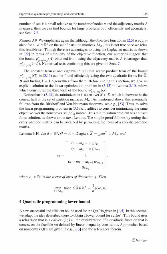
number of sets k is small relative to the number of nodes n and the adjacency matrix Ais sparse, then we can find bounds for large problems both efficiently and accurately;see Sect. 7.2.
Remark 3.9 We emphasize again that although the objective function in (2.5) is equiv-alent for all d ∈ R
n on the set of partition matricesMm , this is not true once we relaxthis feasible set. Though there are advantages to using the Laplacian matrix as shownin [22] in terms of simplicity of the objective function, our numerics suggest thatthe bound p∗projeig(A) obtained from using the adjacency matrix A is stronger thanp∗projeig(−L). Numerical tests confirming this are given in Sect. 7.
The constant term α and eigenvalue minimal scalar product term of the boundp∗projeig(G) in (3.13) can be found efficiently using the two quadratic forms for G,
B and finding k − 1 eigenvalues from them. Before ending this section, we give anexplicit solution to the linear optimization problem in (3.13) in Lemma 3.10, below,which constitutes the third term of the bound p∗projeig(G).
Notice that in (3.13), theminimization is taken over X ∈ D, which is shown to be theconvex hull of the set of partition matricesMm . As mentioned above, this essentiallyfollows from the Birkhoff and Von Neumann theorems, see e.g., [23]. Thus, to solvethe linear programming problem in (3.13), it suffices to consider minimizing the sameobjective over the nonconvex setMm instead. This minimization problem has a closedform solution, as shown in the next Lemma. The simple proof follows by noting thatevery partition matrix can be obtained by permuting the rows of a specific partitionmatrix.
Lemma 3.10 Let d ∈ Rn, G = A − Diag(d), X = 1
n emT ∈Mm and
v0 =
⎡
⎢⎢⎢⎢⎢⎢⎣
(n − mk − m1)em1
(n − mk − m2)em2
...
(n − mk − mk−1)emk−10emk
⎤
⎥⎥⎥⎥⎥⎥⎦
,
where e j ∈ Rj is the vector of ones of dimension j . Then
minX∈Mm
trace GX BXT = 1
n〈Ge, v0〉−.
4 Quadratic programming lower bound
Anew successful and efficient bound used for theQAP is given in [1,5]. In this section,we adapt the idea described there to obtain a lower bound for cut(m). This bound usesa relaxation that is a convex QP, i.e., the minimization of a quadratic function that isconvex on the feasible set defined by linear inequality constraints. Approaches basedon nonconvex QPs are given in e.g., [13] and the references therein.
123
346 T. K. Pong et al.
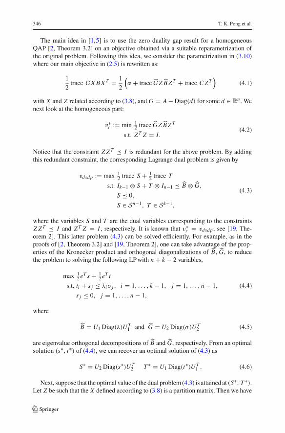
The main idea in [1,5] is to use the zero duality gap result for a homogeneousQAP [2, Theorem 3.2] on an objective obtained via a suitable reparametrization ofthe original problem. Following this idea, we consider the parametrization in (3.10)where our main objective in (2.5) is rewritten as:
1
2trace GXBXT = 1
2
(α + trace G Z BZT + trace CZT
)(4.1)
with X and Z related according to (3.8), and G = A−Diag(d) for some d ∈ Rn . We
next look at the homogeneous part:
v∗r := min 12 trace G Z BZT
s.t. ZT Z = I.(4.2)
Notice that the constraint Z ZT � I is redundant for the above problem. By addingthis redundant constraint, the corresponding Lagrange dual problem is given by
vdsdp := max 12 trace S + 1
2 trace T
s.t. Ik−1 ⊗ S + T ⊗ In−1 � B ⊗ G,
S � 0,
S ∈ Sn−1, T ∈ Sk−1,
(4.3)
where the variables S and T are the dual variables corresponding to the constraintsZ ZT � I and ZT Z = I , respectively. It is known that v∗r = vdsdp; see [19, The-orem 2]. This latter problem (4.3) can be solved efficiently. For example, as in theproofs of [2, Theorem 3.2] and [19, Theorem 2], one can take advantage of the prop-erties of the Kronecker product and orthogonal diagonalizations of B, G, to reducethe problem to solving the following LPwith n + k − 2 variables,
max 12e
T s + 12e
T t
s.t. ti + s j ≤ λiσ j , i = 1, . . . , k − 1, j = 1, . . . , n − 1,
s j ≤ 0, j = 1, . . . , n − 1,
(4.4)
where
B = U1 Diag(λ)UT1 and G = U2 Diag(σ )UT
2 (4.5)
are eigenvalue orthogonal decompositions of B and G, respectively. From an optimalsolution (s∗, t∗) of (4.4), we can recover an optimal solution of (4.3) as
S∗ = U2 Diag(s∗)UT
2 T ∗ = U1 Diag(t∗)UT
1 . (4.6)
Next, suppose that the optimal value of the dual problem (4.3) is attained at (S∗, T ∗).Let Z be such that the X defined according to (3.8) is a partition matrix. Then we have
123
Eigenvalue, quadratic programming, and semidefinite... 347
1
2trace(G Z BZT ) = 1
2vec(Z)T (B ⊗ G) vec(Z)
= 1
2vec(Z)T (B ⊗ G − I ⊗ S∗ − T ∗ ⊗ I )︸ ︷︷ ︸
Q
vec(Z)
+ 1
2trace(Z ZT S∗)+ 1
2trace(T ∗)
= 1
2vec(Z)T Q vec(Z)+ 1
2trace([Z ZT − I ]S∗)+ 1
2trace(S∗)
+ 1
2trace(T ∗)
≥ 1
2vec(Z)T Q vec(Z)+ 1
2trace(S∗)+ 1
2trace(T ∗),
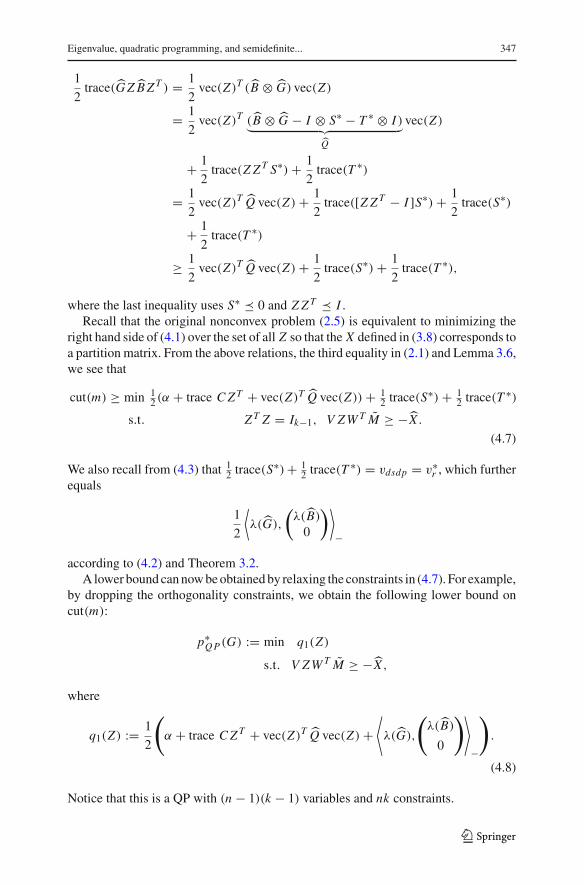
where the last inequality uses S∗ � 0 and Z ZT � I .Recall that the original nonconvex problem (2.5) is equivalent to minimizing the
right hand side of (4.1) over the set of all Z so that the X defined in (3.8) corresponds toa partition matrix. From the above relations, the third equality in (2.1) and Lemma 3.6,we see that
cut(m) ≥ min 12 (α + trace CZT + vec(Z)T Q vec(Z))+ 1
2 trace(S∗)+ 1
2 trace(T∗)
s.t. ZT Z = Ik−1, V ZWT M ≥ −X .
(4.7)
We also recall from (4.3) that 12 trace(S
∗)+ 12 trace(T
∗) = vdsdp = v∗r , which furtherequals
1
2
⟨λ(G),
(λ(B)
0
)⟩
−
according to (4.2) and Theorem 3.2.A lower bound cannowbeobtainedby relaxing the constraints in (4.7). For example,
by dropping the orthogonality constraints, we obtain the following lower bound oncut(m):
p∗QP (G) := min q1(Z)
s.t. V ZWT M ≥ −X ,
where
q1(Z) := 1
2
(
α + trace CZT + vec(Z)T Q vec(Z)+⟨
λ(G),
(λ(B)
0
)⟩
−
)
.
(4.8)
Notice that this is a QP with (n − 1)(k − 1) variables and nk constraints.
123
348 T. K. Pong et al.
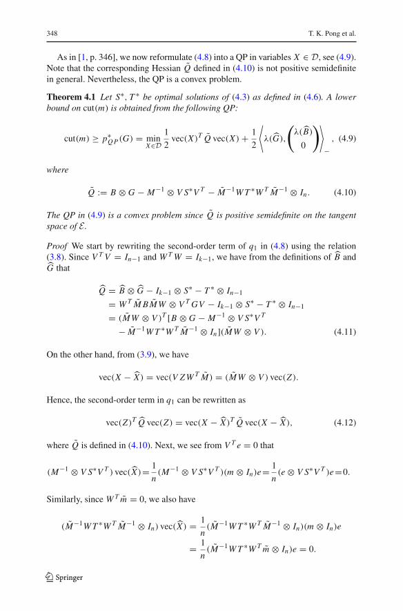
As in [1, p. 346], we now reformulate (4.8) into a QP in variables X ∈ D, see (4.9).Note that the corresponding Hessian Q defined in (4.10) is not positive semidefinitein general. Nevertheless, the QP is a convex problem.
Theorem 4.1 Let S∗, T ∗ be optimal solutions of (4.3) as defined in (4.6). A lowerbound on cut(m) is obtained from the following QP:
cut(m) ≥ p∗QP (G) = minX∈D
1
2vec(X)T Q vec(X)+ 1
2
⟨
λ(G),
(λ(B)
0
)⟩
−, (4.9)
where
Q := B ⊗ G − M−1 ⊗ V S∗V T − M−1WT ∗WT M−1 ⊗ In . (4.10)
The QP in (4.9) is a convex problem since Q is positive semidefinite on the tangentspace of E .
Proof We start by rewriting the second-order term of q1 in (4.8) using the relation(3.8). Since V T V = In−1 and WTW = Ik−1, we have from the definitions of B andG that
Q = B ⊗ G − Ik−1 ⊗ S∗ − T ∗ ⊗ In−1= WT MBMW ⊗ V TGV − Ik−1 ⊗ S∗ − T ∗ ⊗ In−1= (MW ⊗ V )T [B ⊗ G − M−1 ⊗ V S∗V T
− M−1WT ∗WT M−1 ⊗ In](MW ⊗ V ). (4.11)
On the other hand, from (3.9), we have
vec(X − X) = vec(V ZWT M) = (MW ⊗ V ) vec(Z).
Hence, the second-order term in q1 can be rewritten as
vec(Z)T Q vec(Z) = vec(X − X)T Q vec(X − X), (4.12)
where Q is defined in (4.10). Next, we see from V T e = 0 that
(M−1 ⊗ V S∗V T ) vec(X)= 1
n(M−1 ⊗ V S∗V T )(m ⊗ In)e= 1
n(e ⊗ V S∗V T )e=0.
Similarly, since WT m = 0, we also have
(M−1WT ∗WT M−1 ⊗ In) vec(X) = 1
n(M−1WT ∗WT M−1 ⊗ In)(m ⊗ In)e
= 1
n(M−1WT ∗WT m ⊗ In)e = 0.
123
Eigenvalue, quadratic programming, and semidefinite... 349
Combining the above two relations with (4.12), we obtain further that
vec(Z)T Q vec(Z) = vec(X)T Q vec(X)− 2 vec(X)T [B ⊗ G] vec(X)
+ vec(X)[B ⊗ G] vec(X)
= vec(X)T Q vec(X)− 2 trace GX BXT + α.
For the first two terms of q1, proceeding as in (3.16), we have
α + trace CZT = −α + 2 trace GX BXT .
Furthermore, recall from Lemma 3.6 that with X and Z related by (3.8), X ∈ D if,and only if, V ZWT M ≥ −X .
The conclusion in (4.9) now follows by substituting the above expressions into(4.8).
Finally, from (4.11) we see that Q is positive semidefinite when restricted to therange of MW ⊗ V . This is precisely the tangent space of E . ��
Although the dimension of the feasible set in (4.9) is slightly larger than the dimen-sion of the feasible set in (4.8), the former feasible set is much simpler. Moreover, asmentioned above, even though Q is not positive semidefinite in general, it is whenrestricted to the tangent space of E . Thus, as in [5], one may apply the Frank–Wolfealgorithm on (4.9) to approximately compute the QP lower bound p∗QP (G) for prob-lems with huge dimension.
Since Q � 0, it is easy to see from (4.8) that p∗QP (G) ≥ p∗projeig(G). This inequal-ity is not necessarily strict. Indeed, if G = −L , then C = 0 and α = 0 in (4.8). Sincethe feasible set of (4.8) contains the origin, it follows from this and the definition ofp∗projeig(−L) that p∗QP (−L) = p∗projeig(−L). Despite this, as we see in the numericsSect. 7, we have p∗QP (A) > p∗projeig(A) for most of our numerical experiments. Ingeneral, we still do not know what conditions will guarantee p∗QP (G) > p∗projeig(G).
5 Semidefinite programming lower bounds
In this section, we study the SDP relaxation constructed from the various equalityconstraints in the representation in (2.1) and the objective function in (2.4).
One way to derive an SDP relaxation for (2.5) is to start by considering a suitableLagrangian relaxation, which is itself an SDP. Taking the dual of this Lagrangianrelaxation then gives an SDP relaxation for (2.5); see [28,29] for the development forthe QAP and GP cases, respectively. Alternatively, we can also obtain the same SDPrelaxation directly using the well-known lifting process, e.g., [3,17,24,28,29]. In thisapproach, we start with the following equivalent quadratically constrained quadraticproblems to (2.5):
123
350 T. K. Pong et al.
cut(m) = min 12 trace GXBXT = min 1
2 trace GXBXT
s.t. X ◦ X = X, s.t. X ◦ X = x0X,
‖Xe − e‖2 = 0, ‖Xe − x0e‖2 = 0,
‖XT e − m‖2 = 0, ‖XT e − x0m‖2 = 0,
X :i ◦ X : j = 0, ∀i �= j, X :i ◦ X : j = 0, ∀i �= j,
XT X − M = 0, XT X − M = 0,
diag(XXT )− e = 0. diag(XXT )− e = 0,
x20 = 1.
(5.1)
Here: G = A − Diag(d), d ∈ Rn ; the first equality follows from the fifth equality
in (2.1), and we add x0 and the constraint x20 = 1 to homogenize the problem. Notethat if x0 = −1 at the optimum, then we can replace it with x0 = 1 by changing thesign X ← −X while leaving the objective value unchanged. We next linearize thequadratic terms in (5.1) using the matrix
YX :=(
1
vec(X)
)
(1 vec(X)T ).
Then YX � 0 and is rank one. The objective function becomes
1
2trace GXBXT = 1
2trace LGYX ,
where
LG :=[0 0
0 B ⊗ G
]
. (5.2)
By removing the rank one restriction on YX and using a general symmetric matrixvariable Y rather than YX , we obtain the following SDP relaxation:
cut(m) ≥ p∗SDP (G) := min 12 trace LGY
s.t. arrow (Y ) = e0,
trace D1Y = 0,
trace D2Y = 0,
GJ (Y ) = 0,
DO(Y ) = M,
De(Y ) = e,
Y00 = 1,
Y � 0,
(5.3)
123
Eigenvalue, quadratic programming, and semidefinite... 351
where the rows and columns of Y ∈ Skn+1 are indexed from 0 to kn, and e0 is the first(0th) unit vector. The notation used for describing the constraints above is standard;see, for example, [28]. For the convenience of the readers, we also describe them indetail in the “Appendix”.
From the details in the “Appendix”, we have that both D1 and D2 are positivesemidefinite. From the constraints trace DiY = 0, i = 1, 2 we conclude that thefeasible set of (5.3) has no strictly feasible (positive definite) point Y � 0. Numericaldifficulties can arise when an interior-point method is directly applied to a problemwhere strict feasibility, Slater’s condition, fails. Nonetheless, as in [28], we can find asimple matrix in the relative interior of the feasible set and use its structure to project(and regularize) the problem into a smaller dimension. This is achieved by finding amatrix V with range equal to the intersection of the nullspaces of D1 and D2. This iscalled facial reduction, [4,7]. Let Vj ∈ R
j×( j−1), V Tj e = 0, e.g.,
Vj :=
⎡
⎢⎢⎢⎢⎢⎢⎣
1 0 . . . . . . 0
0 1 . . . . . . 0
0 0 1 . . . 0
. . . . . . . . . . . . 1
−1 . . . . . . −1 −1
⎤
⎥⎥⎥⎥⎥⎥⎦
j×( j−1)
.
and let
V :=[
1 01nm ⊗ en Vk ⊗ Vn
]
,
where en is the vector of ones of dimension n. Then the range of V is equal to the rangeof (any) Y ∈ relint F , the relative interior of the minimal face, and we can faciallyreduce (5.3) using the substitution
Y = V Z V T ∈ Skn+1, Z ∈ S(k−1)(n−1)+1.
The facially reduced SDP is then given by
cut(m) ≥ p∗SDP (G) = min 12 trace V T LG V Z
s.t. arrow (V Z V T ) = e0
G J (V Z V T ) = G J (e0eT0 )
DO(V Z V T ) = M
De(V Z V T ) = e
Z � 0, Z ∈ S(k−1)(n−1)+1,
(5.4)
where we let J := J ∪ (0, 0).We now present our final SDP relaxation (SDP f inal) in Theorem 5.1 below and dis-
cuss some of its properties. This relaxation is surprisingly simple/strong with many of
123
352 T. K. Pong et al.
the constraints in (5.4) redundant. In particular, we show that the problem is indepen-dent of the choice of d ∈ R
n in constructing G. We also show that the two constraintsusingDO ,De are redundant in the SDP relaxation (SDP f inal). This answers affirma-tively the question posed in [28] on whether these constraints were redundant in theSDP relaxation for the GP.
Theorem 5.1 The facially reduced SDP (5.4) is equivalent to the single equality con-strained problem
cut(m) ≥ p∗SDP (G) = min 12 trace
(V T LG V
)Z
s.t. G J (V Z V T ) = G J (e0eT0 ) (SDP f inal)
Z � 0, Z ∈ S(k−1)(n−1)+1.
The dual program is
max 12W00
s.t. V TG J (W )V � V T LG V .(5.5)
Both primal and dual satisfy Slater’s constraint qualification and the objective functionis independent of the d ∈ R
n chosen to form G.
Proof It is shown in [28] that the second constraint in (5.4) along with Z � 0 impliesthat the arrow constraint holds, i.e., the arrow constraint is redundant. It only remainsto show that the last two equality constraints in (5.4) are redundant. First, the gangsterconstraint using the linear transformation G J implies that the blocks in Y = V Z V T
satisfy diag Y(i j) = 0 for all i �= j , where Y respects the block structure describedin (9.3). Next, we note that Di � 0, i = 1, 2 and Y � 0. Therefore, the Schurcomplement of Y00 implies that
Y � Y0:kn,0YT0:kn,0.
Writing v1 := Y0:kn,0 and X = Mat(Y1:kn,0), we see further that
0 = trace(DiY ) ≥ trace(Div1vT1 ) =
{‖Xe − e‖2 if i = 1,
‖XT e − m‖2 if i = 2.
This together with the arrow constraints show that trace Y(i i) = ∑nij=(i−1)n+1 Y j0 =
mi . Thus, DO(V Z V T ) = M holds. Similarly, one can see from the above and thearrow constraint that De(V Z V T ) = e holds.
The conclusion about Slater’s constraint qualification for (SDP f inal) follows from[28, Theorem 4.1], which discussed the primal SDP relaxations of the GP. That relax-ation has the same feasible set as (SDP f inal). In fact, it is shown in [28] that
Z=⎡
⎣1 0
0 1n2(n−1) (nDiag(mk−1)− mk−1mT
k−1)⊗ (nIn−1 − En−1)
⎤
⎦∈S(k−1)(n−1)+1+ ,
123
Eigenvalue, quadratic programming, and semidefinite... 353
where mTk−1 = (m1, . . . ,mk−1) and En−1 is the n − 1 square matrix of ones, is a
strictly feasible point for (SDP f inal). The right-hand side of the dual (5.5) differsfrom the dual of the SDP relaxation of the GP. However, let
W =[
α 0
0 (Ek − Ik)⊗ In
]
.
From the proof of [28, Theorem 4.2] we see that G J (W ) = W and
−V TG J (W )V = V T (−W )V
=[1 mT ⊗ eT /n
0 V Tk ⊗ V T
n
][−α 0
0 ((Ik − Ek)⊗ In
][1 0
m ⊗ e/n Vk ⊗ Vn
]
=[−α + mT (Ik − Ek)m/n (mT (Ik − Ek)Vk)⊗ (eT Vn)/n
(V Tk (Ik − Ek)m)⊗ (V T
n e)/n (V Tk (Ik − Ek)Vk)⊗ (V T
n Vn)
]
=[−α + mT (Ik − Ek)m/n 0
0 (Ik−1 + Ek−1)⊗ (In−1 + En−1)
]
� 0, for sufficiently large − α.
Therefore V TG J (βW )V ≺ V T LG V for sufficiently large −α, β, i.e., Slater’s con-straint qualification holds for the dual (5.5).
Finally, we let Y = V Z V T with Z feasible for (SDP f inal). Then Y satisfies thegangster constraints, i.e., diag Y(i j) = 0 for all i �= j . On the other hand, if we restrictD = Diag(d), then the objective matrix LD has nonzero elements only in the samediagonal positions of the off-diagonal blocks from the application of the Kroneckerproduct B ⊗ Diag(d). Thus, we must have trace LDY = 0. Consequently, for alld ∈ R
n ,
trace(V T LG V
)Z= trace LGV Z V T = trace LGY = trace L AY = trace V L AV
T Z .
��We next present two useful properties for finding/recovering approximate partition
matrix solutions X from a solution Y of (SDP f inal).
Proposition 5.2 Suppose that Y is feasible for (SDP f inal). Let v1 = Y1:kn,0 and(v0 vT2
)Tdenote a unit eigenvector of Y corresponding to the largest eigenvalue.
Then X1 := Mat(v1) ∈ E ∩ N . Moreover, if v0 �= 0, then X2 := Mat( 1v0
v2) ∈ E .Furthermore, if, Y ≥ 0, then v0 �= 0 and X2 ∈ N .
Proof The fact that X1 ∈ E was shown in the proof of Theorem 5.1. That X1 ∈ Nfollows from the arrow constraint. We now prove the results for X2. Suppose first thatv0 �= 0. Then
Y � λ1(Y )
(v0
v2
)(v0
v2
)T
.
123
354 T. K. Pong et al.
Using this and the definitions of Di and X2, we see further that
0 = trace(DiY ) ≥{
λ1(Y )v20‖X2e − e‖2, if i = 1,
λ1(Y )v20‖XT2 e − m‖2, if i = 2.
(5.6)
Since λ1(Y ) �= 0 and v0 �= 0, it follows that X2 ∈ E .Finally, suppose that Y ≥ 0.We claim that any eigenvector
(v0 vT2
)Tcorresponding
to the largest eigenvalue must satisfy:
1. v0 �= 0;2. all entries have the same sign, i.e., v0v2 ≥ 0.
From these claims, it would follow immediately that X2 = Mat(v2/v0) ∈ N .To prove these claims, we note first from the classical Perron–Fröbenius theory,
e.g., [6], that the vector(|v0| |v2|T
)Tis also an eigenvector corresponding to the largest
eigenvalue.2 Letting χ := Mat(v2) and proceeding as in (5.6), we conclude that
‖χe − v0e‖2 = 0 and ‖|χ |e − |v0|e‖2 = 0.
The second equality implies that v0 �= 0. If v0 > 0, then for all i = 1, . . . , n, we have
k∑
j=1χi j = v0 =
k∑
j=1|χi j |,
showing that χi j ≥ 0 for all i , j , i.e., v2 ≥ 0. If v0 < 0, one can show similarly thatv2 ≤ 0. Hence, we have also shown v0v2 ≥ 0. This completes the proof. ��
6 Feasible solutions and upper bounds
In the abovewehave presented several approaches for finding lower bounds for cut(m).In addition, we have found matrices X that approximate the bound and satisfy some ofthe graph partitioning constraints. Specifically, we obtain two approximate solutionsXA, XL ∈ E in (3.19), an approximate solution to (4.8) which can be transformed intoan n × k matrix via (3.9), and the X1, X2 described in Proposition 5.2. We now usethese to obtain feasible solutions (partition matrices) and thus obtain upper bounds.
We show below that we can find the closest feasible partition matrix X to a givenapproximatematrix X using linear programming,where X is found, for example, usingthe projected eigenvalue, QP or SDP lower bounds. Note that (6.1) is a transportationproblem and therefore the optimal X in (6.1) can be found in strongly polynomial time(O(n2)), see e.g., [25,26].
2 Indeed, if Y is irreducible, the largest in magnitude eigenvalue is positive and a singleton and the corre-sponding eigenspace is the span of a positive vector. Hence the conclusion follows. For a reducible Y , due tosymmetry of Y , it is similar via permutation to a block diagonal matrix whose blocks are irreducible matri-ces. Thus, we can apply the same argument to conclude similar results for the eigenspace corresponding tothe largest magnitude eigenvalue.
123
Eigenvalue, quadratic programming, and semidefinite... 355
Theorem 6.1 Let X ∈ E be given. Then the closest partition matrix X to X in Fröbe-nius norm can be found by using the simplex method to solve the linear program
min − trace X T Xs.t. Xe = e,
XT e = m,
X ≥ 0.
(6.1)
Proof Observe that for any partition matrix X , trace XT X = n. Hence, we have
minX∈Mm
‖X − X‖2F = trace(X T X)+ n + 2 minX∈Mm
trace(−X T X
).
The result now follows from this and the fact that Mm = ext(D), as stated in (2.1).(This is similar to what is done in [29].) ��
7 Numerical tests
In this section, we provide empirical comparisons for the lower and upper boundspresented above. All the numerical tests are performed in MATLAB version R2012aon a single node of the COPS cluster at University of Waterloo. It is an SGI XE340system, with two 2.4 GHz quad-core Intel E5620 Xeon 64-bit CPUs and 48 GBRAM,equipped with SUSE Linux Enterprise server 11 SP1.
7.1 Random tests with various sizes
In this subsection, we compare the bounds on structured graphs. These are formedby first generating k disjoint cliques (of sizes m1, . . . ,mk , randomly chosen from{2, ..., imax + 1}). We join the first k − 1 cliques to every node of the kth clique. Wethen add u0 edges between the first k − 1 cliques, chosen uniformly at random fromthe complement graph. In our tests, we set u0 = �ec p�, where ec is the number ofedges in the complement graph and 0 ≤ p < 1. By construction, u0 ≥ cut(m).
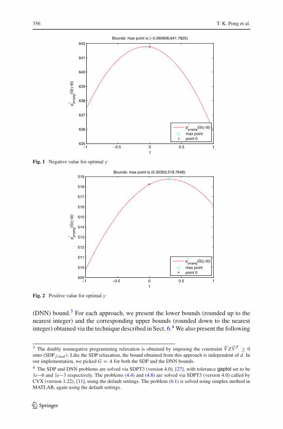
First, we note the following about the eigenvalue bounds. The two Figs. 1 and 2show the difference in the projected eigenvalue bounds from using A − γ Diag(d)
for a random d ∈ Rn on two structured graphs. This is typical of what we saw in
our tests, i.e., that the maximum bound is near γ = 0. We had similar results for thespecific choice d = Ae. This empirically suggests that using A would yield a betterprojected eigenvalue lower bound. This phenomenon leads us to use A in subsequenttests below.
In Table 1, we consider small instances where k = 4, 5, p = 20% and imax = 10.Weconsider the projected eigenvalue boundswithG = −L (eig−L ) andG = A (eigA),the QP bound with G = A, the SDP bound and the doubly nonnegative programming
123
356 T. K. Pong et al.
−1 −0.5 0 0.5 1635
636
637
638
639
640
641
642
γ
p* proj
eig(G
( γ d
))
Bounds: max point is (−0.060606,641.7825)
p*projeig
(G(γ d))
max pointpoint 0
Fig. 1 Negative value for optimal γ
−1 −0.5 0 0.5 1509
510
511
512
513
514
515
516
517
518
519
γ
p* proj
eig(G
(γ d
))
Bounds: max point is (0.30303,518.7646)
p*projeig
(G(γ d))
max pointpoint 0
Fig. 2 Positive value for optimal γ
(DNN) bound.3 For each approach, we present the lower bounds (rounded up to thenearest integer) and the corresponding upper bounds (rounded down to the nearestinteger) obtained via the technique described in Sect. 6.4 We also present the following
3 The doubly nonnegative programming relaxation is obtained by imposing the constraint V Z V T ≥ 0onto (SDP f inal ). Like the SDP relaxation, the bound obtained from this approach is independent of d. Inour implementation, we picked G = A for both the SDP and the DNN bounds.4 The SDP and DNN problems are solved via SDPT3 (version 4.0), [27], with tolerance gaptol set to be1e−6 and 1e−3 respectively. The problems (4.4) and (4.8) are solved via SDPT3 (version 4.0) called byCVX (version 1.22), [11], using the default settings. The problem (6.1) is solved using simplex method inMATLAB, again using the default settings.
123
Eigenvalue, quadratic programming, and semidefinite... 357
Table 1 Results for small structured graphs
Data Lower bounds Upper bounds Gap
n k |E | u0 eig−L eigA QP SDP DNN eig−L eigA QP SDP DNN
31 4 362 25 21 22 24 23 25 68 102 25 36 25 0.0000
18 4 86 16 13 14 15 16 16 22 35 16 19 16 0.0000
29 5 229 44 32 37 40 39 44 76 74 44 53 44 0.0000
41 5 453 91 76 84 86 86 91 159 162 101 125 102 0.0521
Table 2 Results for medium-sized structured graphs
Data Lower bounds Upper bounds Gap
n k |E | u0 eig−L eigA QP SDP eig−L eigA QP SDP
69 8 1077 317 249 283 290 281 516 635 328 438 0.0615
114 8 3104 834 723 785 794 758 1475 1813 834 1099 0.0246
85 8 2164 351 262 319 327 320 809 384 367 446 0.0576
116 10 3511 789 659 725 737 690 1269 2035 796 1135 0.0385
104 10 2934 605 500 546 554 529 1028 646 631 836 0.0650
78 10 1179 455 358 402 413 389 708 625 494 634 0.0893
129 12 3928 1082 879 988 1001 965 1994 1229 1233 1440 0.1022
120 12 3102 1009 833 913 926 893 1627 1278 1084 1379 0.0786
126 12 2654 1305 1049 1195 1218 1186 1767 1617 1361 1736 0.0554
measure of accuracy, defined as
Gap = best upper bound− best lower bound
best upper bound+ best lower bound. (7.1)
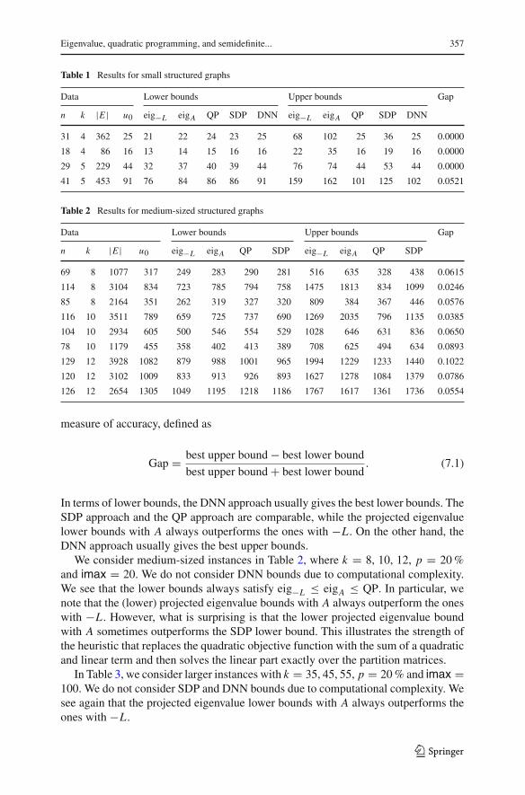
In terms of lower bounds, the DNN approach usually gives the best lower bounds. TheSDP approach and the QP approach are comparable, while the projected eigenvaluelower bounds with A always outperforms the ones with −L . On the other hand, theDNN approach usually gives the best upper bounds.
We consider medium-sized instances in Table 2, where k = 8, 10, 12, p = 20%and imax = 20. We do not consider DNN bounds due to computational complexity.We see that the lower bounds always satisfy eig−L ≤ eigA ≤ QP. In particular, wenote that the (lower) projected eigenvalue bounds with A always outperform the oneswith −L . However, what is surprising is that the lower projected eigenvalue boundwith A sometimes outperforms the SDP lower bound. This illustrates the strength ofthe heuristic that replaces the quadratic objective function with the sum of a quadraticand linear term and then solves the linear part exactly over the partition matrices.
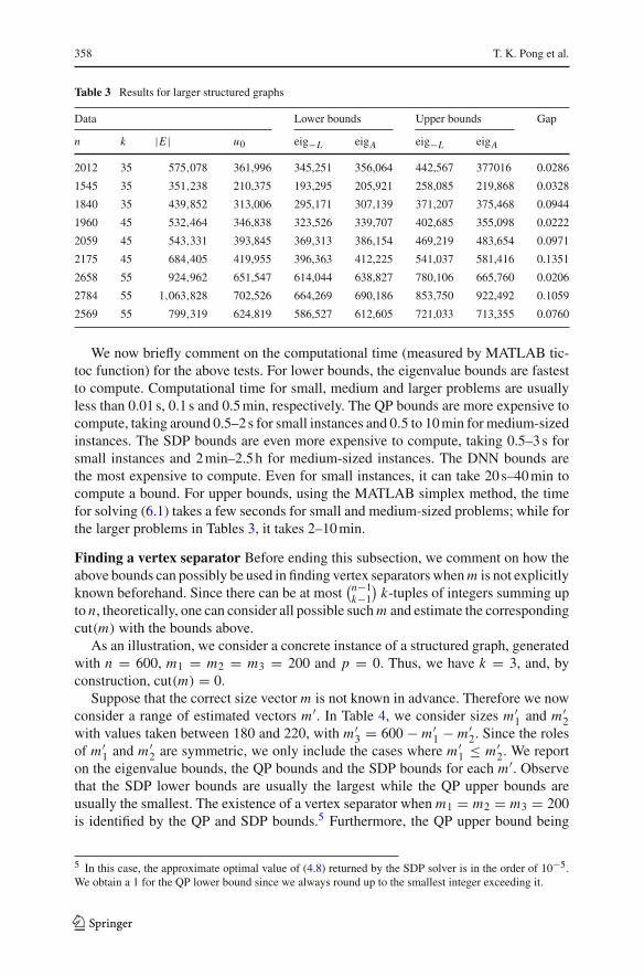
In Table 3, we consider larger instances with k = 35, 45, 55, p = 20% and imax =100. We do not consider SDP and DNN bounds due to computational complexity. Wesee again that the projected eigenvalue lower bounds with A always outperforms theones with −L .
123
358 T. K. Pong et al.
Table 3 Results for larger structured graphs
Data Lower bounds Upper bounds Gap
n k |E | u0 eig−L eigA eig−L eigA
2012 35 575,078 361,996 345,251 356,064 442,567 377016 0.0286
1545 35 351,238 210,375 193,295 205,921 258,085 219,868 0.0328
1840 35 439,852 313,006 295,171 307,139 371,207 375,468 0.0944
1960 45 532,464 346,838 323,526 339,707 402,685 355,098 0.0222
2059 45 543,331 393,845 369,313 386,154 469,219 483,654 0.0971
2175 45 684,405 419,955 396,363 412,225 541,037 581,416 0.1351
2658 55 924,962 651,547 614,044 638,827 780,106 665,760 0.0206
2784 55 1,063,828 702,526 664,269 690,186 853,750 922,492 0.1059
2569 55 799,319 624,819 586,527 612,605 721,033 713,355 0.0760
We now briefly comment on the computational time (measured by MATLAB tic-toc function) for the above tests. For lower bounds, the eigenvalue bounds are fastestto compute. Computational time for small, medium and larger problems are usuallyless than 0.01 s, 0.1 s and 0.5min, respectively. The QP bounds are more expensive tocompute, taking around 0.5–2s for small instances and 0.5 to 10min formedium-sizedinstances. The SDP bounds are even more expensive to compute, taking 0.5–3s forsmall instances and 2min–2.5h for medium-sized instances. The DNN bounds arethe most expensive to compute. Even for small instances, it can take 20s–40min tocompute a bound. For upper bounds, using the MATLAB simplex method, the timefor solving (6.1) takes a few seconds for small and medium-sized problems; while forthe larger problems in Tables 3, it takes 2–10min.
Finding a vertex separator Before ending this subsection, we comment on how theabove bounds can possibly be used in finding vertex separators whenm is not explicitlyknown beforehand. Since there can be at most
(n−1k−1)k-tuples of integers summing up
to n, theoretically, one can consider all possible suchm and estimate the correspondingcut(m) with the bounds above.
As an illustration, we consider a concrete instance of a structured graph, generatedwith n = 600, m1 = m2 = m3 = 200 and p = 0. Thus, we have k = 3, and, byconstruction, cut(m) = 0.
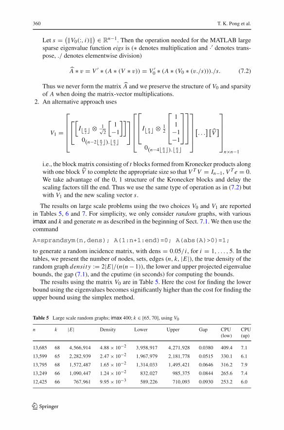
Suppose that the correct size vector m is not known in advance. Therefore we nowconsider a range of estimated vectors m′. In Table 4, we consider sizes m′1 and m′2with values taken between 180 and 220, with m′3 = 600 − m′1 − m′2. Since the rolesof m′1 and m′2 are symmetric, we only include the cases where m′1 ≤ m′2. We reporton the eigenvalue bounds, the QP bounds and the SDP bounds for each m′. Observethat the SDP lower bounds are usually the largest while the QP upper bounds areusually the smallest. The existence of a vertex separator when m1 = m2 = m3 = 200is identified by the QP and SDP bounds.5 Furthermore, the QP upper bound being
5 In this case, the approximate optimal value of (4.8) returned by the SDP solver is in the order of 10−5.We obtain a 1 for the QP lower bound since we always round up to the smallest integer exceeding it.
123
Eigenvalue, quadratic programming, and semidefinite... 359
Table 4 Results for medium-sized graph without an explicitly known m
Data Lower bounds Upper bounds
m′1 m′2 eig−L eigA QP SDP eig−L eigA QP SDP
180 180 −3600 −2400 −2400 −1800 2520 32,400 0 540
180 200 −1922 −1281 −1270 −949 2538 36,000 0 3240
180 220 −99 −66 −16 0 3600 39,600 3600 4312
200 200 0 0 1 0 2200 39,801 0 0
200 220 2074 2716 2759 4000 4000 40,000 4398 11, 832
220 220 4400 5867 5867 8400 8400 40,241 8400 12, 916
zero for the cases (m′1,m′2) = (180, 180), (180, 200) also indicates the existence of avertex separator.
7.2 Large sparse projected eigenvalue bounds
We assume that n k. The projected eigenvalue bound in Theorem 3.7 in (3.13) iscomposed of a constant term, aminimal scalar product of k−1 eigenvalues and a linearterm. The constant term and linear term are trivial to evaluate and essentially take noCPU time. The evaluation of the k − 1 eigenvalues of B is also efficient and accurateas the matrix is small and symmetric. The only significant cost is the evaluation ofthe largest k − 2 eigenvalues and the smallest eigenvalue of G. In our test below, weuse G = A for simplicity. This choice is also justified by our numerical results in theprevious subsection and the observation from Figs. 1 and 2.
We use the MATLAB eigs command for the k − 1 eigenvalues of V T AV forthe lower bound. Since the corresponding (6.1) has much larger dimension than weconsidered in the previous subsection, we turn to IBM ILOG CPLEX version 12.4(MATLAB interface) with default settings to solve for the upper bound. We use theMATLAB tic-toc function to time the routine for finding the lower bound, and reportoutput.time from the function cplexlp.m as the cputime for finding the upper bound.
We use two different choices V0 and V1 for the matrix V in (3.7).
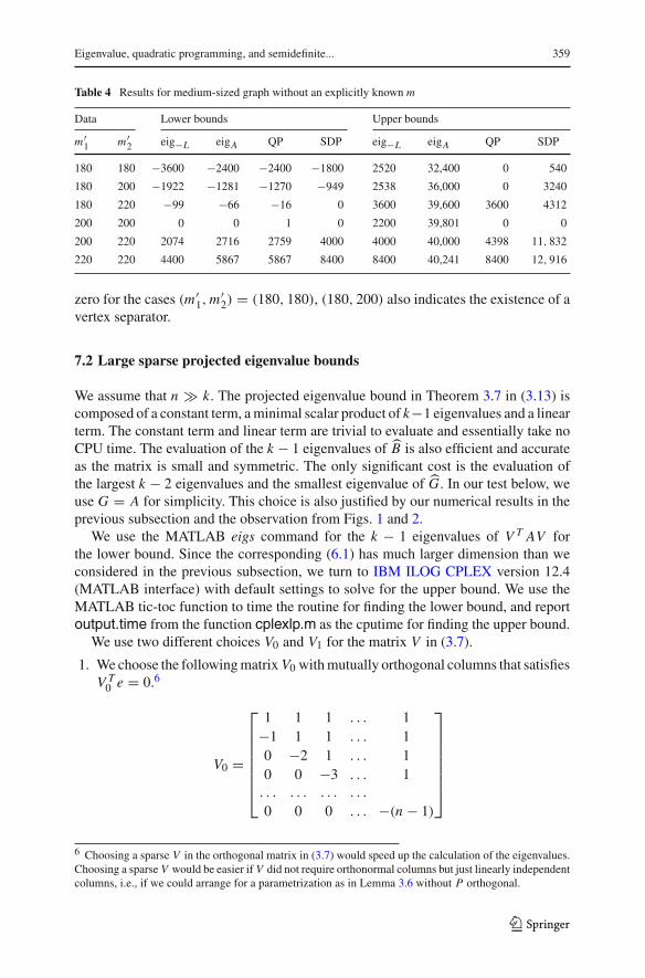
1. We choose the followingmatrix V0 withmutually orthogonal columns that satisfiesV T0 e = 0.6
V0 =
⎡
⎢⎢⎢⎢⎢⎢⎣
1 1 1 . . . 1−1 1 1 . . . 10 −2 1 . . . 10 0 −3 . . . 1. . . . . . . . . . . .
0 0 0 . . . −(n − 1)
⎤
⎥⎥⎥⎥⎥⎥⎦
6 Choosing a sparse V in the orthogonal matrix in (3.7) would speed up the calculation of the eigenvalues.Choosing a sparse V would be easier if V did not require orthonormal columns but just linearly independentcolumns, i.e., if we could arrange for a parametrization as in Lemma 3.6 without P orthogonal.
123
360 T. K. Pong et al.
Let s = (‖V0(:, i)‖) ∈ R
n−1. Then the operation needed for the MATLAB largesparse eigenvalue function eigs is (∗ denotes multiplication and ·′ denotes trans-pose, ./ denotes elementwise division)
A ∗ v = V ′ ∗ (A ∗ (V ∗ v)) = V ′0 ∗ (A ∗ (V0 ∗ (v./s)))./s. (7.2)
Thus we never form the matrix A and we preserve the structure of V0 and sparsityof A when doing the matrix-vector multiplications.
2. An alternative approach uses
V1 =
⎡
⎢⎢⎢⎢⎣
⎡
⎣
[I� n2 � ⊗ 1√
2
[1−1]]
0(n−2� n2 �),� n2 �
⎤
⎦
⎡
⎢⎢⎢⎢⎣
⎡
⎢⎢⎣I� n4 � ⊗ 1
2
⎡
⎢⎢⎣
11−1−1
⎤
⎥⎥⎦
⎤
⎥⎥⎦
0(n−4� n4 �),� n4 �
⎤
⎥⎥⎥⎥⎦
[. . .] [V]
⎤
⎥⎥⎥⎥⎦
n×n−1
i.e., the block matrix consisting of t blocks formed fromKronecker products alongwith one block V to complete the appropriate size so that V T V = In−1, V T e = 0.We take advantage of the 0, 1 structure of the Kronecker blocks and delay thescaling factors till the end. Thus we use the same type of operation as in (7.2) butwith V1 and the new scaling vector s.
The results on large scale problems using the two choices V0 and V1 are reportedin Tables 5, 6 and 7. For simplicity, we only consider random graphs, with variousimax and k and generatem as described in the beginning of Sect. 7.1. We then use thecommand
A=sprandsym(n,dens); A(1:n+1:end)=0; A(abs(A)>0)=1;
to generate a random incidence matrix, with dens = 0.05/ i , for i = 1, . . . , 5. In thetables, we present the number of nodes, sets, edges (n, k, |E |), the true density of therandom graph densi ty := 2|E |/(n(n−1)), the lower and upper projected eigenvaluebounds, the gap (7.1), and the cputime (in seconds) for computing the bounds.
The results using the matrix V0 are in Table 5. Here the cost for finding the lowerbound using the eigenvalues becomes significantly higher than the cost for finding theupper bound using the simplex method.
Table 5 Large scale random graphs; imax 400; k ∈ [65, 70], using V0
n k |E | Density Lower Upper Gap CPU(low)
CPU(up)
13,685 68 4,566,914 4.88× 10⁻² 3,958,917 4,271,928 0.0380 409.4 7.1
13,599 65 2,282,939 2.47× 10⁻² 1,967,979 2,181,778 0.0515 330.1 6.1
13,795 68 1,572,487 1.65× 10⁻² 1,314,033 1,495,421 0.0646 316.2 7.9
13,249 66 1,090,447 1.24× 10⁻² 832,027 985,375 0.0844 265.6 7.4
12,425 66 767,961 9.95× 10⁻³ 589,226 710,093 0.0930 253.2 6.0
123
Eigenvalue, quadratic programming, and semidefinite... 361
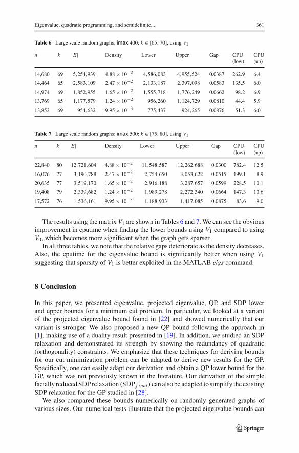
Table 6 Large scale random graphs; imax 400; k ∈ [65, 70], using V1
n k |E | Density Lower Upper Gap CPU(low)
CPU(up)
14,680 69 5,254,939 4.88× 10⁻² 4,586,083 4,955,524 0.0387 262.9 6.4
14,464 65 2,583,109 2.47× 10⁻² 2,133,187 2,397,098 0.0583 135.5 6.0
14,974 69 1,852,955 1.65× 10⁻² 1,555,718 1,776,249 0.0662 98.2 6.9
13,769 65 1,177,579 1.24× 10⁻² 956,260 1,124,729 0.0810 44.4 5.9
13,852 69 954,632 9.95× 10⁻³ 775,437 924,265 0.0876 51.3 6.0
Table 7 Large scale random graphs; imax 500; k ∈ [75, 80], using V1
n k |E | Density Lower Upper Gap CPU(low)
CPU(up)
22,840 80 12,721,604 4.88× 10⁻² 11,548,587 12,262,688 0.0300 782.4 12.5
16,076 77 3,190,788 2.47× 10⁻² 2,754,650 3,053,622 0.0515 199.1 8.9
20,635 77 3,519,170 1.65× 10⁻² 2,916,188 3,287,657 0.0599 228.5 10.1
19,408 79 2,339,682 1.24× 10⁻² 1,989,278 2,272,340 0.0664 147.3 10.6
17,572 76 1,536,161 9.95× 10⁻³ 1,188,933 1,417,085 0.0875 83.6 9.0
The results using the matrix V1 are shown in Tables 6 and 7.We can see the obviousimprovement in cputime when finding the lower bounds using V1 compared to usingV0, which becomes more significant when the graph gets sparser.
In all three tables, we note that the relative gaps deteriorate as the density decreases.Also, the cputime for the eigenvalue bound is significantly better when using V1suggesting that sparsity of V1 is better exploited in the MATLAB eigs command.
8 Conclusion
In this paper, we presented eigenvalue, projected eigenvalue, QP, and SDP lowerand upper bounds for a minimum cut problem. In particular, we looked at a variantof the projected eigenvalue bound found in [22] and showed numerically that ourvariant is stronger. We also proposed a new QP bound following the approach in[1], making use of a duality result presented in [19]. In addition, we studied an SDPrelaxation and demonstrated its strength by showing the redundancy of quadratic(orthogonality) constraints. We emphasize that these techniques for deriving boundsfor our cut minimization problem can be adapted to derive new results for the GP.Specifically, one can easily adapt our derivation and obtain a QP lower bound for theGP, which was not previously known in the literature. Our derivation of the simplefacially reducedSDP relaxation (SDP f inal) can also be adapted to simplify the existingSDP relaxation for the GP studied in [28].
We also compared these bounds numerically on randomly generated graphs ofvarious sizes. Our numerical tests illustrate that the projected eigenvalue bounds can
123
362 T. K. Pong et al.
be found efficiently for large scale sparse problems and that they compare well againstother more expensive bounds on smaller problems. It is surprising that the projectedeigenvalue bounds using the adjacencymatrix A are both cheap to calculate and strong.
Acknowledgments T. K. Pong was supported partly by a research grant from Hong Kong PolytechnicUniversity. He was also supported as a PIMS postdoctoral fellow at Department of Computer Science,University of British Columbia, Vancouver, during the early stage of the preparation of the manuscript.Research of H. Sun supported by an Undergraduate Student Research Award from The Natural Sciencesand Engineering Research Council of Canada. Research of N. Wang supported by The Natural Sciencesand Engineering Research Council of Canada and by the U.S. Air Force Office of Scientific Research. H.Wolkowincz: Research supported in part by The Natural Sciences and Engineering Research Council ofCanada and by the U.S. Air Force Office of Scientific Research.
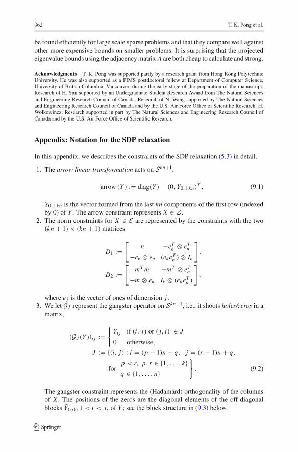
Appendix: Notation for the SDP relaxation
In this appendix, we describes the constraints of the SDP relaxation (5.3) in detail.
1. The arrow linear transformation acts on Skn+1,
arrow (Y ) := diag(Y )− (0,Y0,1:kn)T , (9.1)
Y0,1:kn is the vector formed from the last kn components of the first row (indexedby 0) of Y . The arrow constraint represents X ∈ Z .
2. The norm constraints for X ∈ E are represented by the constraints with the two(kn + 1)× (kn + 1) matrices
D1 :=[
n −eTk ⊗ eTn−ek ⊗ en (ekeTk )⊗ In
]
,
D2 :=[
mTm −mT ⊗ eTn−m ⊗ en Ik ⊗ (eneTn )
]
,
where e j is the vector of ones of dimension j .3. We let GJ represent the gangster operator on Skn+1, i.e., it shoots holes/zeros in a
matrix,
(GJ (Y ))i j :={Yi j if (i, j) or ( j, i) ∈ J
0 otherwise,
J := {(i, j) : i = (p − 1)n + q, j = (r − 1)n + q,
forp < r, p, r ∈ {1, . . . , k}q ∈ {1, . . . , n}
}
. (9.2)
The gangster constraint represents the (Hadamard) orthogonality of the columnsof X . The positions of the zeros are the diagonal elements of the off-diagonalblocks Y(i j), 1 < i < j, of Y ; see the block structure in (9.3) below.
123
Eigenvalue, quadratic programming, and semidefinite... 363
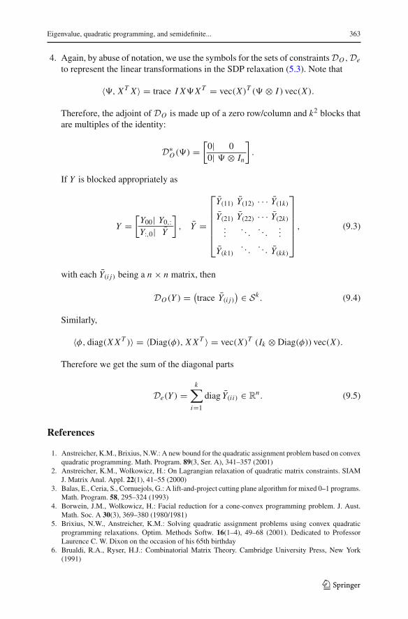
4. Again, by abuse of notation, we use the symbols for the sets of constraintsDO ,De
to represent the linear transformations in the SDP relaxation (5.3). Note that
〈�, XT X〉 = trace I X�XT = vec(X)T (� ⊗ I ) vec(X).
Therefore, the adjoint of DO is made up of a zero row/column and k2 blocks thatare multiples of the identity:
D∗O(�) =[0| 00| � ⊗ In
].
If Y is blocked appropriately as
Y =[Y00| Y0,:Y:,0| Y
], Y =
⎡
⎢⎢⎢⎢⎢⎣
Y(11) Y(12) · · · Y(1k)
Y(21) Y(22) · · · Y(2k)...
. . .. . .
...
Y(k1). . .
. . . Y(kk)
⎤
⎥⎥⎥⎥⎥⎦
, (9.3)
with each Y(i j) being a n × n matrix, then
DO(Y ) = (trace Y(i j)) ∈ Sk . (9.4)
Similarly,
〈φ, diag(XXT )〉 = 〈Diag(φ), XXT 〉 = vec(X)T (Ik ⊗ Diag(φ)) vec(X).
Therefore we get the sum of the diagonal parts
De(Y ) =k∑
i=1diag Y(i i) ∈ R
n . (9.5)
References
1. Anstreicher, K.M., Brixius, N.W.: A new bound for the quadratic assignment problem based on convexquadratic programming. Math. Program. 89(3, Ser. A), 341–357 (2001)
2. Anstreicher, K.M., Wolkowicz, H.: On Lagrangian relaxation of quadratic matrix constraints. SIAMJ. Matrix Anal. Appl. 22(1), 41–55 (2000)
3. Balas, E., Ceria, S., Cornuejols, G.: A lift-and-project cutting plane algorithm for mixed 0–1 programs.Math. Program. 58, 295–324 (1993)
4. Borwein, J.M., Wolkowicz, H.: Facial reduction for a cone-convex programming problem. J. Aust.Math. Soc. A 30(3), 369–380 (1980/1981)
5. Brixius, N.W., Anstreicher, K.M.: Solving quadratic assignment problems using convex quadraticprogramming relaxations. Optim. Methods Softw. 16(1–4), 49–68 (2001). Dedicated to ProfessorLaurence C. W. Dixon on the occasion of his 65th birthday
6. Brualdi, R.A., Ryser, H.J.: Combinatorial Matrix Theory. Cambridge University Press, New York(1991)
123
364 T. K. Pong et al.
7. Cheung, Y.-L., Schurr, S.,Wolkowicz, H.: Preprocessing and regularization for degenerate semidefiniteprograms. In: Bailey, D.H., Bauschke, H.H., Borwein, P., Garvan, F., Thera, M., Vanderwerff, J.,Wolkowicz, H. (eds.) Computational andAnalytical Mathematics. In Honor of Jonathan Borwein’s60thBirthday. Springer Proceedings in Mathematics & Statistics, vol. 50, pp. 225–276. Springer, NewYork (2013)
8. de Klerk, E., Nagy, M.E., Sotirov, R.: On semidefinite programming bounds for graph bandwidth.Optim. Methods Softw. 28(3), 485–500 (2013)
9. Demmel, J.W.: Applied Numerical Linear Algebra. Society for Industrial and Applied Mathematics(SIAM), Philadelphia (1997)
10. Falkner, J., Rendl, F., Wolkowicz, H.: A computational study of graph partitioning. Math. Program.66(2, Ser. A), 211–239 (1994)
11. Grant, M., Boyd, S., Ye, Y.: Disciplined convex programming. In: Global Optimization. NonconvexGlobal Optimization, vol. 84, pp. 155–210. Springer, New York (2006)
12. Hadley, S.W., Rendl, F.,Wolkowicz, H.: A new lower bound via projection for the quadratic assignmentproblem. Math. Oper. Res. 17(3), 727–739 (1992)
13. Hager, W.W., Hungerford, J.T.: A continuous quadratic programming formulation of the vertex sepa-rator problem. Report, University of Florida, Gainesville (2013)
14. Hoffman, A.J., Wielandt, H.W.: The variation of the spectrum of a normal matrix. Duke Math. 20,37–39 (1953)
15. Horn,R.A., Johnson,C.R.:MatrixAnalysis.CambridgeUniversityPress,Cambridge (1990).Correctedreprint of the 1985 original
16. Lewis, R.H.: Yet another graph partitioning problem is NP-Hard. Report. arXiv:1403.5544 [cs.CC](2014)
17. Lovász, L., Schrijver, A.: Cones of matrices and set-functions and 0–1 optimization. SIAM J. Optim.1(2), 166–190 (1991)
18. Martí, R., Campos, V., Piñana, E.: A branch and bound algorithm for the matrix bandwidth minimiza-tion. Eur. J. Oper. Res. 186(2), 513–528 (2008)
19. Povh, J., Rendl, F.: Approximating non-convex quadratic programs by semidefinite and copositiveprogramming. In: KOI 2006—11th International Conference on Operational Research, pp. 35–45.Croatian Operational Research Review, Zagreb (2008)
20. Rendl, F., Wolkowicz, H.: Applications of parametric programming and eigenvalue maximization tothe quadratic assignment problem. Math. Program. 53(1, Ser. A), 63–78 (1992)
21. Rendl, F., Wolkowicz, H.: A projection technique for partitioning the nodes of a graph. Ann. Oper. Res.58, 155–179 (1995). Applied mathematical programming and modeling, II (APMOD 93) (Budapest,1993)
22. Rendl, F., Lisser, A., Piacentini, M.: Bandwidth, vertex separators and eigenvalue optimization. In:Discrete Geometry and Optimization. The Fields Institute for Research in Mathematical Sciences.Communications Series. pp. 249–263. Springer, New York (2013)
23. Schrijver, A.: Theory of Linear and Integer Programming. Wiley-Interscience Series in Discrete Math-ematics. Wiley, Chichester (1986)
24. Sherali, H.D., Adams, W.P.: Computational advances using the reformulation-linearization technique(rlt) to solve discrete and continuous nonconvex problems. Optima 49, 1–6 (1996)
25. Tardos, E.: A strongly polynomial algorithm to solve combinatorial linear programs. Oper. Res. 34(2),250–256 (1986)
26. Tardos, E.: Strongly polynomial and combinatorial algorithms in optimization. In: Proceedings of theInternational Congress of Mathematicians, Vol. I, II (Kyoto, 1990), pp. 1467–1478. MathematicalSociety of Japan, Tokyo (1991)
27. Tütüncü, R.H., Toh, K.C., Todd, M.J.: Solving semidefinite-quadratic-linear programs using SDPT3.Math. Program. 95(2, Ser. B), 189–217 (2003). Computational semidefinite and second order coneprogramming: the state of the art
28. Wolkowicz, H., Zhao, Q.: Semidefinite programming relaxations for the graph partitioning problem.Discrete Appl. Math. 96(97), 461–479 (1999). Selected for the special Editors’ Choice, Edition 1999
29. Zhao, Q., Karisch, S.E., Rendl, F., Wolkowicz, H.: Semidefinite programming relaxations for thequadratic assignment problem. J. Comb. Optim. 2(1), 71–109 (1998). Semidefinite programmingand interior-point approaches for combinatorial optimization problems (Fields Institute, Toronto, ON,1996)
123