.. '"

I i I ! ~ I l

I

\ 1 ...

This microfiche was produced from documents received for inclusion in the NCJRS data base. Since NCJRS cann.ot exercise'

control over the physical condition of the documents submitted, th" individual frame quality will vary. The resolution chart on tbis frame may be used to evaluate .thedocument quality . . ,- .. "-_ ... _._,_., .. ,. .. ""'~I'

, l,

1.0 111112

.5

2.2

1.1 --------- 1111/1.8

111111.25 111111.4 111111.6'

MICROCOPY RESOLUTION TEST CHART . NATIONAL BUREAU OF STANOARDS-J963-A .. ----------------~ L_.,

(j

t\ f;' ,I

, 'J

"I ;'1 ",1 4

,,'I , ... \ i /~ ,j

:: ! ,':I ;d :j ,j '[ " ¥

\ ,'/ 1

~J ' .. '

Microiilminl procedures used to' create this fiche comply with

the standards set forth in 41CFR 101·11.504

Points of view or oPinions stated' in this doculilent are those of the authorls) and do not represent the official position or policies of the U.S. Department of Justice.

U.S. DEPARTMENT OF JUSTICE LAW ENFORCEMENT ASSISTANCE ADMINISTRATION' NATION'AL CRIMINAL JUSTICE REFERENCE SERVICE WASHINGTON, D.C. 20531

h

. I

I 9/16/75 \ , L. ,... ,"

" t~*~:~,~,.c.·'

, ,t,

REPRINTEP FROM URBAN ANALYSIS ..

VOLUME 2 :", 19.7'4

·f . ( ".

I.'. '.

\ \.,

" '~ ,

PLANNING IN Qo.~BAN .PUB.LI C SAFETY ,.'. \'\ ' ...

NAT IONALSCIENCI: II FOUNDAT IONGRANT"G 13800 4 .. ';. '. RESEAR.CH APPLI ED TO NATIONAL NEEDS ',;.

. D I.VI S ION OF soc I AL~YS TEMSAND HI)MAR.;R ESOURC.ES

'. i .. 'OPERATJONSRESEARCH 'CENTER.' MAssAcHUSETTS . INSTITUTE OF . TEC/-fNOt.OG'{ .'. !. ',:9AMBJ{I PG,E)MASSAJ~,US~TTS 02134,,' ..... .

, , .; ... ". ',.',

···.·.··,················t·,'.··.·········· .. ···••••· '1'-,"', :',;.' " ::"

" • ,": '. ."', : I :,' ~: .: , .... " , " ~ .,'

, "," '., "

.. ) ,''.,1. "". .

.'~·;.·~')~:k4·~'·;~h~~~~~~L,~ .

If you have issues viewing or accessing this file contact us at NCJRS.gov.

Urban Analysis, 1974, Vol. 2, pp. 51-91 © 1974 Gordon and Breach Science Publishers Ltd. Printed in Great Britain

} III U_S~r~!jY~.""EQlj~(:t.".SJ~Gtq r Red es i 9 n ~ - '-,

in District 4· in Boston ___ ~~;::,,~:,"".::'7.-:;.-~.s ,;:, .... ,'-"'," '::" :~~: _>r" y' " .'.&.

RICHARD C. LARSON

Associate Professor of Urban Studies and Electrical Engineering, Room 24-215, r4~ Massachusetts Institute of Technology, Cambridge, Massachusetts 02139

i (Received October 31, 1973)

A newly developed computer program, based on a multiserver queuing model, is applied to the problem oLpolice sector redesign in part of the City of Boston. Using commonly available data describing patterns of calls for service, travel times, dispatching strategies, and other factors, the model computes numerical values of several operational performance measures. These include mean travel times, workloads, and fractions of dispatches that are cross-sector.

Using 1971 call-for-service data, a case example is worked out requiring four iterations between the planner and the model for District 4 inBoston. Prior to the iterations, an attempt is made to describe the logic or intuition or rules-of-thumb that are used in arriving at various sector designs.

Members of a Resource Allocation Task Force at the Boston Police Department utilized several concepts of this methodology in a massive manpower reallocation program, "The Maximum Response and Patrol Plan", implemented by Commissioner Robert J. diGrazia in September 1973. .

This paper describes a computer model that estimates the operating per­formance of radio-dispatched police patrol cars in the field, given certain data regarding distribution of calls for service, service times, travel times, dis­patching strategies, and spatial distribution of patrol units while on patrol. Although the model has several potential uses, the author feels that its primary immediate application will be in the redesign of police patrol sectors and similar service regions for other public safety systems, such as ambulance dispatch areas. Our purpose in this paper is not to present technical details of the model (this is done in Larson (1973] and in other documentst), but

t A first preliminary computer implementation of the model used here is reported by Campbell (1972). A somewhat more complex model, which allows the dispatcher's prefer­ences for patrol units to vary, depending on which regions in the city are relatively congested, is reported by Jarvis (1973). A user's manual for the model used in this paper, developed by Larson (1973), is currently being written.

51

52 R. C. LARSON

rather to illustrate in a nontechnical way how the model may be used for police redesign in an actual operating environment. Our case example deals with Police District 4 in Boston. In part, this choice was motivated by the activities of the Task Force 011 Patrol Manpower Allocation in the Boston Police Department, which in July 1973 selected District 4 for trial imple­mentation of a new manpower allocation and sector design program.

Before presenting the details of the case example, we briefly review some of the obj-ectives of police sector design, we describe the input data that are used in the example, and we summarize some useful rules-of-thumb in sector design. A concluding section summarizes the methodology and discusses current implementation activities in the Boston-Cambridge area.

For those not familiar with police terminology, an abbreviated glossary is presented in Table I.

'FABLE I

Glossary of police terms relate,d to the BostoI'! case example

(Words set in italics are defined elsewhere in the gIOSS<lry.)

Call for service A communication to the police originating from a citizcn, an alarm system, a police offi(:er, or other detector, reporting an incident that requires on-scene police assistance.

Command (or District) An area or region comprising several.sectors that is administratively distinct, usually having a station-house used as a base of operations. Often called precincts or (as in Boston) districts. A patrol officer is usually assigned to one command for a period of time. Dispatch assignments are nearly always intra-command assignments.

Dispatch assignment A directive by the dispatcher to a patrol unit assigning the unit to respond to the scene of a reported incident or call for service.

Dispatcher An individual who has responsibility for assigning available radio-dispatchable patroilinits to reported incidents.

Effective travel speed That speed which, if constantly maintained over the path of a response journey, would result in the same travel time as that actually experienced by the respondingpatroilinit.

Flying A term applied to a patrol unit responding frequently to calls oU'lside its home sector.

Hazard formula A summation of crime statistics, geographical statistics, and other factors thought to be important in determining the need for patrol III/its in a region, each factor multiplied by a weighting indicating its subjective importance.

. ..

POLICE SECTOR REDESIGN 53 Home sector

The sector in which a patrol IlIIit is assigned to perform prevel/tive patrol.

Intersector (or cross-sector) assignment A dispatch assignment to a sector other than the unit's home sector.

Overlapping sectors Sectors that at least partially share common regions.

Patrol allocation

The entire process of determining the total required number of patrol units, their spatial arid temporal assignments, and rules governing their operation.

Patrol status

The condition of a patrol unit, particularly pertaining to dispatch availability. In some police departmcnts (he dispatch status of a patrol unit is restricted to one of (wo possibilities: available or unavailable; in others, finer distinc,tions are made, including such possibilities as meal break, auto maintenance, patrol-initiated action, station-house, or type of incident currently being serviced.

Patrol unit

A patrol car, scooter, or wagon and its assigned police officer(s); or a radio-dispatchable footpatrolman.

Preventive patrol

An activity undertaken by a patrol unit, in which the unit tours an area, with the officer(s) checking for crime hazards (for example, open doors and windows) and attempting to intercept any crimes while in progress.

Reporting area

A subarea within a command, typically no more than a few city blocks in size, that is used as the smallest geographical unit for aggregating statistics on the spatial distributions of calls for service and prevel/til'e patrol coverage.

Sector (or Beat)

An area in which one patrol UI/it has (usually exclusive) preventive patrol responsibility.

Sector identity

A term applied to an officer's personal commitment to maintain public order and provide effective police service within his home sector.

Service time

The total "off the air" time per call for service for a patrolllliit. Includes travel time, on­scene time and possibly related off-scene time.

Travel time

The time required for the dispatchedpatl'olunit to travel to the scene of the reported incident.

Utilization factor

The fraction of time a patrol unit is unavailable to respond to dispatch l'eqU\~sts. In this paper it is assumed that a unit can only be unavailable because of call-servicing duties. Sometimes called utilization rate.

Workload Same as utilization factor.

54 R. C. LARSON

BRIEF DESCRIPTION OF POLICE PATROL OPERATIONt

Our focus is on the radio-dispatched police patrol force. Each radio­dispatched unit (usually a patrol car, wagon or scooter) is assigned a primary area of patrol responsibility, which we refer to as the unit's sector, although "beat", "car area", and other terms are used, depending on local tradition.

One primary duty of the unit is to traverse its sector performing "crime preventive patrol", the purpose of which is to prevent crime by removing crime hazards and to deter crime by posing the threat of apprehension. Usually high crime rate regions within the sector receive relatively greater preventive patrol attention than low crime rate regions.

The second primary duty of the unit is to respond to calls for police service. These are usually generated by citizens calling the police emergency number. After the necessary information is obtained, a police dispatcher assigns or dispatches a patrol unit ,to the scene of the call. It is important to note that a call for service interrupts preventive patrol, since rapid response is considered to be of higher priority than general patrolling.

When possible, a call for service is usually assigned to the unit whose sector contains the location of the call. However, if this unit is already busy servicing a previolls call, then the dispatcher assigns an out-of-sector unit, resulting in an intersector dispatch. From a planning point of view, intra­sector dispatches are usually preferred to intersector dispatches because (1) they most often result in shorter travel times and (2) they enhance the officer's identity with his own sector by providing citizen contact within the sector at locations requiring police service.

At any given time the dispatcher has only a fixed pool of units that can respond to calls in each command (or "precinct", "district", or "division"), which is an administrative grouping of sectors. Most commands have a centrally located stationhouse to which all patrolmen report for a briefing ("roll call") prior to entering their cars and travelling to their sectors to commence a tour of duty (usually lasting eight hours).t The New York City Police Department averaged nine sectors per command (precinct) in 1969. Should the need arise, usually each unit can be dispatched to any point within its command. If, unfortunately, all units in a command are simul­taneously busy when a call arrives, then the dispatcher enters the call in queue for later dispatch. There are very few intercommand dispatches, and our sector design procedures wi11neglect them.

t The description of police patrol operation in this section is necessarily brief and focuses primarily on issues tllat relate to sector design. A much more complete picture including circumstances in which the dispatch-patrol system deviates from its normal set of operating procedures, is found in Larson (1972), Chapter 1.

t The stationhouse also houses the command's supervisory officers, serves as a receiving point for individuals arrested for crimes within the command, and provides a location for citizen "wa.lk-in" complaints.

...

..

POLICE SECTOR REDESIGN 55

For purposes of sector design, it is necessary to know the statistical ?atterns of demands for police service (for both calls and preventive patrol) ll1 subareas throughout the command. The subareas, or police reporting areas, or geographical cells should be significantly smaller than sectors so that sectors can be designed as combinations of subareas. Various cities use census tracts, city blocks, or specially designed police subareas as their police reporting areas. In our work, we will assume that each police sector is a particular com­bination of reporting areas.

Now, for a specific command, the two basic questions in sector design are

1) How many units should be assigned to the command during a particular time period?

2) How should the sectors of these units be designed? '

W~ will assume that the time period for each sector design is sufficiently s~o~t so that the statistical patterns of demands for police service do not slgm~cantly change during the period; but sufficiently long so that we can meanmgfully examine "average" behavior of the patrol units in the command. In most cities this period of time would range from two to six hours in dura­tion, depen~i~g o~ the time of day and 'season of the year. We ,recogni;e that many CitIes stIpulate as an administrative constraint that the sector plan must be fixed over a twenty-four hour period; while the model we use: in this paper. can be app~ied under this constraint (by calculating average system behaVIOr unde~ .dIfferent demand conditions but identical sector designs, and then combmmg results), for simplicity we focus on one time period under one set of demand conditions.

OBJECTIVES IN SECTOR DESIGN

We. now ask ~~e question, "What,' 'are reasonable objectives in designing polIce ~ec~~rs? The answers are dIfficult, depend on departmental policies and pnontIes, and are often mutually conflicting. Several first-order con-siderations come to mind: '.

1) There should not be marked disparities in workloads among the radio­dispatched patrol units. In other words, it would be inadvisable for one unit to work (on calls for service) a significant fraction of time greater than another unit. In part, this consideration is motivated by patrolmen's morale and efficiency considerations, equity, and perhaps by negotiated labor contract

• requirements. More fundamentally, a large workload imbalance implies an equally large, but reversed, imbalance in preventive patrol coverage. This latter problem is compounded by the fact that sectors whose units are busier

56 R. C. LARSON

than average often require the greatest amount of preventive patrol attention. Hereafter we use the term "workload balancing requirell1ent" to refer to these considerations. (Workload balancing would not apply to patrol super­visor cars or other such specialized units.)

2) The sector design should not be such that the average command-wide tral'el time is markedly above the minimum possible. In other words, the value of average travel time should be considered when evaluating alternative sector designs, although travel time minimization by itself is not a single primary objective. We refer to this as the "command-wide travel time requirement" .

3) To the extent controllable by sector designs, there should not be marked inequities in accessibility to police service in various parts of the command. That is, it would be undesirable if police consistently reached some neighbor­hoods within two minutes, while other neighborhoods experience 10 minute travel times. However, geographical considerations make it virtually im­possible to equalize travel times to ali areas, and all we can hope to do is make variations among travel times tolerably small. We refer to this as the "equity of accessibility requirement".

4) To the extent controllable by sector design, the number of cross-sector dispatches should be minimized. Continually dispatc,hing units outside of their own sector reduces the chance of an officer establishing a strong identity with his own sector, increases travel time, and may result in sending an officer to an area in which he is unfamiliar with the street pattern, as well as social mores, and other neighborhood characteristics. We refer to this as the "cross-sector dispatching requirement".

5) There are other considerations that are much less conducive to measure­ment but nevertheless may be equally as important as the above four quantita­tive requirements. For instance, to the extent possible, the police planner may wish to preserve "neighborhood integrity" when designing sectors. Under the assumption that an officer is trying to establish an identity with the citizens of his sector, he may do this best if he has one unified neighbor­hood to deal with rather than two or more neighborhoods artificially divided by sector boundaries. A similar consideration involves the extent to which a new sector plan deviates from the current plan; in many instances, it may be desirable to retain part of the current sector plan in the hope of reducing the amount of time required by patrolmen and dispatchers to learn the details of the new plan.

Undoubtedly each police planner has its own set of issues-some quantita­tively-oriented and some not-that are important in the sector design process. For instance, the well-known police planner O. W. Wilson (1963) focused

POLICE SECTOR REDESIGN 57

heavily on workload balancing in his recommended beat (or sector) design procedures. In most cases, however, regardless of the planner's particular set of issues and their relative priorities, the model described here should be useful in his thinking-primarily because it computes rapidly and effectively many operationally oriented performance measures that come into play in the sector design process, particularly under requirements 1 through 4 above. The model does not "optimize" any performance measures to find the "best" sector design. Rather, the philosophy behind the construction of the model is that in a public service as complex and multifaceted as an urban police depart­ment, the word "optimize" has little meaning. A satisfactory quantitative statement of objectives has been impossible to obtain, and even if it ,,,ere obtainable, one would have to list constraints explicitly-an even more difficult task considering all of the social, political, legal and spatial factors that come into play. Rather, it is felt that a police planner with an intimate knowledge of his own city can be an excellent judge of the qualitative factors that are relevant. USing the computer to calculate the important perform,ance measures, sector design can be viewed as an interative process. First the planner proposes a particular design of sectors and has the computer calculate the resulting values of the performance measures. The planner then incorporates this evidence, including possible workload imbalances and/o.r inequities in accessibility to police service, in with the remainder of his know­ledge of the area under consideration, and decides whether to accept the proposed sector plan or to devise an altered one. In the latter case, the entire process is repeated one, two or several times until a satisfactory sector design is obtained. In this way, good use is made of the planner's talents and the computer's computational power.

SOME USEFUL RULES OF THUMB

In this section we state certain rules of thumb that relate to the sector design problem.- By shedding light on interrelationships among various performance measures, these rules of thumb will assist our intuition in generating and evaluating alternative sector designs.

1) Relatiollship betweell sector area alld sector tralleltime

Other simpler modelst have suggested that allerage travel time withill a sector groll's witll the square root of the area of the sector. For example, if one sector has area 0.25 .;quare mile and another sector has identical geon'letry but four times the area (1.0 square mile), then the average t!'avel time within the second sector is about twice that of the first sector. In practical situations in which sectors have similar geometries and are "not too different" in

t Larson (1972), p. 84.

58 R. C. LARSON

size, this result suggests that average travel times within the sectors will be quite close in value. For instance, if sector B is as much as 40 percent larger (in area) than sector A, the intrasector average travel time of sector B will only be about 18 percent larger than that of sector A.

This rule-of-thumb also implies a probable area of conflicting objectives when trying to balance workloads of units distributed over both densely and sparsely populated areas. A sector design strategy of equalizing intrasector average travel time would dictate designing sectors of approximately equal area, while a strategy of equalizing workloads among units would require relatively larger sectors in the sparse areas. In the first instance, the work­loads of the units in the sparse areas would be considerably less than the workloads of those in the dense areas, but the average intrasector travel times would be about the same. In the second, the average travel times within the larger sectors (in the sparse area) would be greater than those within the smaller sectors (in the dense areas), but the workloads of units would be about the same. This is a conflict that will arise in our case example in District 4.

2) Compactness of sectors The possible geometric designs of a sector are constrained by street patterns, parks, rivers, and other natural and man-made barriers. Within these constraints, however, the police planner will want to arrive at a design that provides appropriate police accessibility to each point within the sector, especially for the sector unit and secondarily for nearby out-of-sector units.

If one focuses on average intrasector travel time as a measure of accessibility within the sector, then one finds that average intrasector travel time is not very sensitive to the exact sector geometry, as long as the sector is reasonably "compact".1" As a rule of thumb, if response speeds do not depend on direction of travel, the greater sector dimension (the "length") should not be more than twice the lesser dimension (the "width"), if reducing mean intrasector travel time is of concern. For example, if we consider two sectors of equal area, each with uniformly distributed calls for service and uniformly distributed preventive patrol coverage, and where the first sector is square and the second is twicG as long as it is wide, then the average intrasector travel time in the second (less compact) sector is only 6 percent greater than that in the first.

If the police planner is concerned with the worst possible situation that could occur in an intrasector response, then he should focus on the maximum possible travel time within the sector. In general, this measure of accessibility is quite sensitive to sector area, overall geometry, and impediments to travel such as one-way streets.t

3) The effect of differing travel speeds In some instances the responding patrol unit can travel significantly faster in one direction than another. For example, in many parts of Manhattan it is possible to travel "uptown" or "downtown" at a much greater speed than "crosstown". The same is true in parts of Boston's Back Bay area where it is usually more rapid to travel parallel to the Charles River (on Beacon Street or Commonwealth Avenue or Boylston 1':tre<:t) than perpendicular to the River (on Berkeley, Exeter or om: of the other "lettered" streets). In such cases the sector design ought to reflect the fact that travel is easier in one direction than another. To keep average intrasector travel time to a level near the minimum, the "longer" sector dimension should correspond. to the direction of greater travel speed and the "shorter" dimension should correspond to the direction of lesser travel speed. Suppose the sector dimensions run East-West and North-South; then the best design (where "best" is measured in terms of average intrasector travel time) is achieved when the average East-West (or West-East) travel time incurred while responding to a call for service within the sector is equal to the average North-South (or South-North) travel time. In Manhattan, where North-South corresponds to uptown-downtown, this would imply that sectors should be longer in the North-South direction and the ratio of the length to the width would be determined so that

1" Larson (1972), p. 84. t See Larson (1972), pp. 82-84, 102-115 fOf additional discussion.

POLICE SECTOR REDESIGN :>9

dUl:ing an averag~ response the patrol unit spends as much time travelling uptown-downtown as It does travellmg crosstown.

4) Relationships between number of cross-sector dispatches and amoullt of time busy all

~al!s for service In p.olice circles it is generally known that as a district becomes buslel,. th~ less the operatIOn of t~e patrol.force resembles the "one-car, one-sector" style of op~latlon that may have been I~ the m1lld of police planner who designed the current secto! plan. As ~ver~ll call-tor-servlce volume within the district increases, it is more likely that a patrol Untt Will service calls outside of his "own" sector because the car assigned to. the sector of the call ~as busy on a previous call at the time of dispatch. What isn't so Widely known .. howeyer, IS the ~xact nature of the relationships between "busyness" and cross-sector dispatchlllg. Here Simpler models again come into plaY1" and suggest that for lo.w to 1I10~erate workload levels the district-wide /raction of dispatches- that are cross-sector dispatches IS at least ~s gr~at as the average fraction of time that units are busy servicing calls. Stated another way, Ifumts are busy an average of 38 percent of the time (on the average) then at least 38 percent of all dispatch assignments will be cross-sector assignments. Further: more, the amount of cross-sector dispatching would be greater than 38 percent if work­loads, wer~ unevenly distributed among units. Thus, another rule-of-thumb: Decreasing I~ork/(/ad unbalances ('~lIally decrea~es the amount of cross-seCtor dispatching. For low to moderate workloads, It IS rarely pOSSible to decrease the fraction of dispatches that are cross­sector belo",:, the ave.rage fraction of time units are busy servicing calls.

Tl?e fractIOn ?f dispatches that are cross-sector tend.s to increase at higher workloads, but It may be slIghtly less than the average fraction of time busy, primarily due to the in­cr.eased number of calls .delayed in queue at. the dispatcher's position; such queued calls ale han~le.~ somewhat differently from calls Immediately dispatched, thereby allowing for the pOSSlblhty of reduced cross-sector dispatching.

5) A patrol unit's workload is /lot equal to its sector's workload This point is ,frequently overlooke~ when des!gni~g sect~rs. Becaus,:: of the frequency of ?ross-sector ~Ispatches, a large fractIOn of a Untt's tIme while responding to calls for service ~s sp~nt outSIde of its own sector and during these periods other units may be dispatched mto It~ sector to cov~r workloads that :ire generated while the sector unit is busy. Thus the followmg.statement IS /lot true: "If sector A generates twice the workload of sector B then patrol U~lt A 'works twice as hard' as patrol unit B."t The relationships between ~ector geome.tnes, sector workloa~s, dispatching strategies, and patrol unit workloads are quite comphcatcd and. are the pnmary motivating force for the model described in this paper. Among other pomts, the model calculations will indicate that a unit's sector can generate belo.w. average workload and y~t the unit can. incur an above-average fraction of time busy servlcl~g calls. Thus the followlllg statement IS also not true: "Equalizing sector workloads reslilts III equalizing patrol unit workloads."

6) The burden of central location A unit whose. sector is situated centrally in its command will be a prime candidate for cross-sector dispatches. Thus,. such a unit is apt to incur a workload greater than that su.ggested by the workload of Its own sector. On the other hand a unit assigned to an out-1~lllg or remote~y-positioned .sector is not likely to be a gooct' candidate for cross-sector dispatches, and Its workload IS apt to be less than that suggested by its sector's internally generated w?rkload. We thus say that the first type of unit suffers from "the burden Of central locatIOn".

From a practical point of view in the sector design process, in order to overcome this problem and thereby balance workloads, the police planner should attempt to design centrally located sectors with less-than-average call-for-service volume and remote sectors

1" Larson (1972), pp. 243-251. + This was a critical underlying assumption in O. W. Wilson's proposed beat design

procedures (Wilson [1963], p. 274).

60 R. C. LARSON

with greater-than-average call-for-service volume. However, the planner usually incurs another trade-off here. As the busy probability of outlying units increases, so does the chance that an out-of-sector unit will have to be dispatched to a call in an outlying sector. Often these responses require lengthy travel times. Thus, the average travel time to outlying points increases as the workload of the sector unit in the outlying sector increases. This is an instance in which equalizing workloads among units increases inequities among neighbor­hoods in accessibility to police service. We will experience this problem also when designing sectors in District 4.

TK~~ MODEL AND ITS DATA REQUIREMENTSt

1 ~le underlying model used in our case example assumes that calls for police ser1{jce arrive at a predictable average hourly rate from each police reporting area, but the exact time of arrival of calls is unpredictable. This is the so­called Poisson input assumption, which has been verified statistically [see, for instance, Larson (1967)]. In response to each call, the dispatcher selects one patrol unit to dispatch to the call, providing at least one is available within. the command. If no "nit is available, the call is entered in queue and assigned later in a first-come, first-served manner.

o mean' 40 minutes t!minutes)

FIGURE 1 Distribution of service time at the scene of an incident.

The time required to service each call, the service time, is the sum of the travel time to the scene, the on-scene time, and possible follow-up off-scene time. The current model assumes that the service time distribution is the same for each unitt This distribution, 1cnown as a negative exponential distribu­tion, is maximum for small service times, and diminishes ~:11oothly for larger

t A more technically detailed description of the model's assumptions is found in Larson (1973).

t Thus, variations in service time that are due solely to variations in travel times of units are ignored.

...

POLICE SECTOR REDESIGN 61

service times. An example is shown in Figure 1 for the case of a 40-minute mean service time. When service is completed on a particular call, it is assumed that the patrol unit is again located in its nome sector, either about to embark on preventive patrol or to be immediately reassigned to a call that has been delayed in queue, in particular, to the call that has been in queue the longest time.

In the foHowing subsections, we detail the data requirements of the lllodel and indicate the numerical values used in the Boston case example.

TABLE II

1971 Number of caUs for service by reporting area

Reporting area Number of calls Reporting area Number of calls

1 1659 36 819 2 2213 37 931 3 1656 38 967 4 888 39 2034 5 709 40 1294 6 1666 41 1412 7 1747 42 959 8 1479 43 2059 9 659 44 1228

10 1383 45 737 11 1350 46 1237 12 837 47 1396 13 618 48 406 14 973 49 1161 15 818 50 863 16 1432 51 451 17 l300 52 947 18 2176 53 645 19 986 54 440 20 1058 55 580 21 512 56 2106 22 1510 57 2703 23 1904 58 1175 24 2632 59 993 25 1299 60 1808 26 1494 61 855 27 675 62 1314 28 907 63 643 29 1171 64 814 30 1219 65 631 31 787 66 419 32 1001 67 950 33 l300 68 1162 34 1263 69 898 35 1049 70 497

--------_______________________ ~ .... ~I.

62 R. C. LARSON

Reporting areas

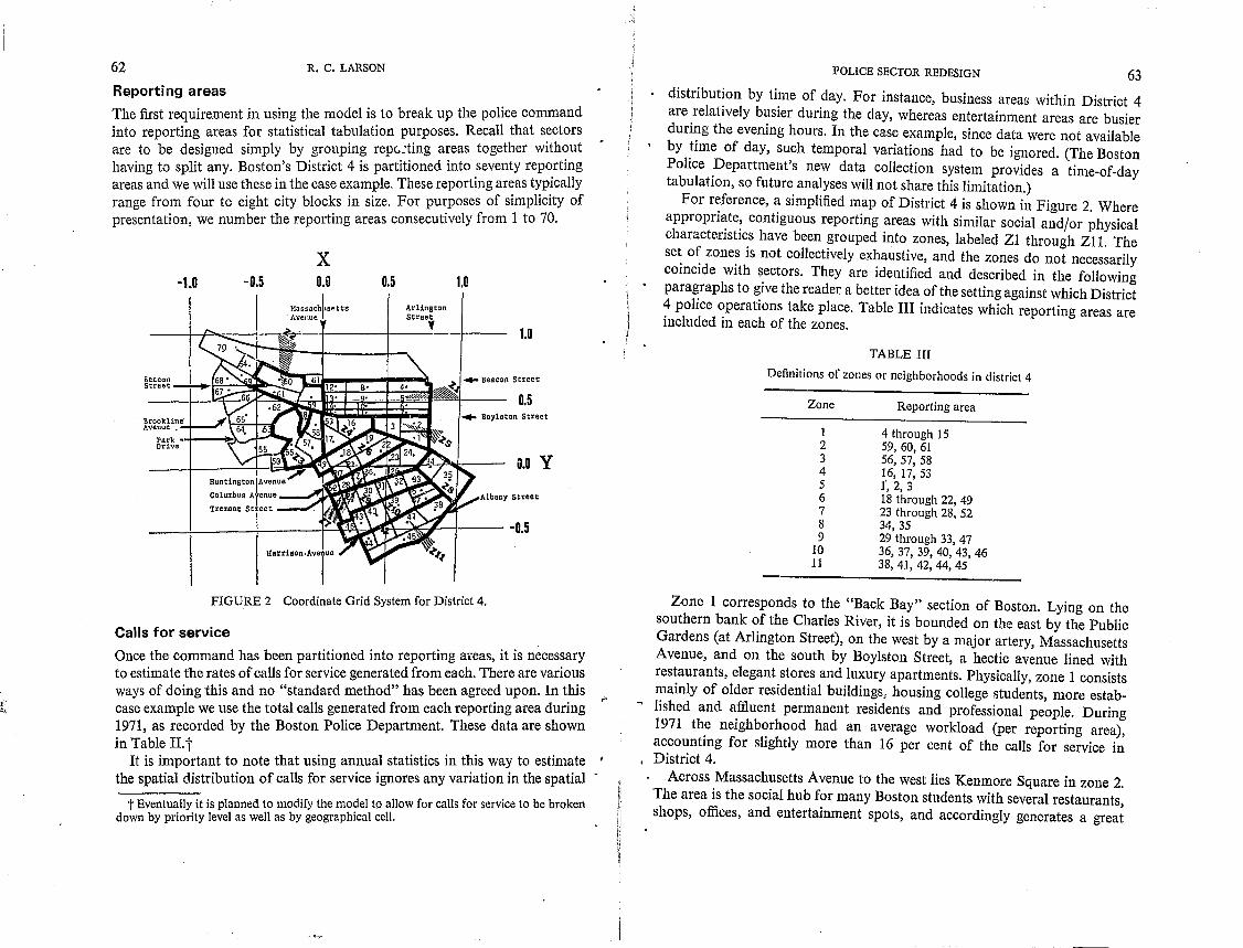
The first requirement in using the model is to break up the police command into reporting areas for statistical tabulation purposes. Recall that sectors are to be designed simply by grouping repc.:ting areas together without having to split any. Boston's District 4 is partitioned into seventy reporting areas and we will use these in the case example. These reporting areas typically range from four to eight city blocks in size. For purposes of simplicity of presentation, we number the reporting areas consecutively from 1 to 70.

-1.0

Brookline· Avenue.

x 0.0

MaSSBcnl-setts Avenue r

Park ·-!--~L--+--W Drive

0.5

Arlington Street y

1.0

1.0

0.0 y

Albany Street

--I----l-----F-~wJf~~rl-- -0.5

FIGURE 2 Coordinate Grid System for District 4.

Calls for service

Once the command has been partitioned into reporting areas, it is necessary to estimate the rates of calls for service generated from each. There are various ways of doing this and no "standard method" has been agreed upon. In this case example we use the total calls generated from each reporting area during 1971, as recorded by the Boston Police Department. These data are shown in Table II. t

It is important to note that using annual statistics in this way to estimate ' the spatial distribution of calls for service ignores any variation in the spatial

t Eventually it is planned to modify the model to allow for calls for service to be broken down by priority level as well as by geographical cell.

POLICE SECTOR REDESIGN 63

distribution by time of day. For instance, business areas within District 4 are relatively busier during the day, whereas entertainment areas are busier during the evening hours. In the case example, since data were not available by ~ime of day, such temporal variations had to be ignored. (The Boston PolIce .Department's new data collection system provides a time-of-day tabulatlOn, so future analyses will not share this limitation.)

For reference, a simplified map of District 4 is shown in Figure 2. Where appropri~te~ contiguous reporting areas with similar social and/or physical charactenstI~s have been grouped into zones, labeled Zl through ZIl. The se: o~ zone~ IS not collectively exhaustive, and the zones do not necessarily comclde wIth ~ectors. They are identified and described in the following paragraphs to gIve the reader a better idea of the setting against which District 4 police operations take place. Table III indicates which reporting areas are included in each of the zones.

TABLE 1Il

Definitions of zones or neighborhoods in district 4

Zone Reporting area

1 2 3 4 5 6 7 8 9

.10 11

4 through 15 59,60,61 56,57,58 16,17,53 r, 2, 3 18 through 22, 49 23 through 28, 52 34,35 29 through 33, 47 36, 37, 39, 40, 43, 46 38,41,42,44,45

Zone 1 corresponds to the "Back Bay" section of Boston. Lying on the southern bank of the Charles River, it is bounded on the east by the Public Gardens (at Arlington Street), on the west by a major artery, Massachusetts Avenue, and on the south by Boylston Street, a hectic avenue lined with restaurants, elegant stores and luxury apartments. Physically, zone 1 consists mainly of older residential buildings, housing college students, more estab-

~ lished and affluent permanent residents and professional people. During 1971 th.e neighb~rhood had an average workload (per reporting area), accountmg for slIghtly more than 16 per cent of the calls for service in

• District 4. Across Massachusetts Avenue to the west lies Kenmore Square in zone 2.

The area is the social hub for many Boston students with several restaurants shops, offices, and entertainment spots, and accordingly generates a grea~

t

64 R. C. LARSON

deal of police work. To the south is zone 3, bordered on the west by the Fenway and Hemenway Street and on the south by Huntington Avenue. The area includes many shops, bars, restaurants and once-elegant row houses. It is a neighborhood in transition with students, elderly whites and poorer blacks vying for apartments. Not surprisingly then, it contains the busiest reporting area in District 4, reporting area 57 with 2703 calls in 1971. The remainder of the District west of Massachusetts Avenue is a quiet residential area generating calls at a rate well below the average.

Moving east across Massachusetts Avenue we reach the triangular zone 4 between Boylston Street and Huntington Avenue. A product of urban renewal, it contains many of Boston's recent architectural "feats" in office complex and hotel construction. In 1971 it generated an average number of caUs. East of zone 4 is the Copley and Park Square area (zone 5). With its entertainment spots, restaurants, hotels and stores, it attracts people, and consequently the police, 5528 times in 1971.

South of Huntington Avenue is a large diverse neighborhood known in Boston as the "South End":, The northern portion (zone 6) is a transition area going from an entertainment and shopping zone (including the Boston Arena) to an older residential neighborhood, with many dead-end streets stopping at the tracks of the Penn-Cen'tral Railroad. This area generated 7403 caUs for service during 1971, a slightly above average rate considering the relatively small area covered.

Moving southward into zone 7 in the true South End, the reporting areas between Columbus Avenue and Tremont Street generated 9858 calls during 1971, a rate 20 percent above the average for seven reporting areas. Many of the old brownstones in this area either are single-owner occupied or have recently undergone renovation for multiple unit rental occupancy. Much of the remaining housing is in a poor state of repair, usually occupied by poorer families. Reporting area 24, in the extreme eastern portion of this area is the second most active reporting area in all of District 4 (reporting 2703 calls in 1971).t . To th~ south and east of reporting area 24 is a business area (zone 8), that In 1971 Included the Boston Herald-Traveller BUilding. This area gel'erated an average number of calls for service for two reporting areas in 1971.

To the west of this area and immediately south of Tremont Street is a number of older residential blocks whose housing stock is in various states ...

t Certain southern and western ~ortions of the South End merge into Boston's Roxbury area, a d~nsely populated, predommantly black, below-average income region. For ease of presentatIOn, howev.::r, we use "South End" as the single label for the collection of southern ' reporting areas in District 4.

t T~ler~ is so~e speCUlation that this figure is inflated since reporting area 24 includes . the DIstrict Statton House, and therefore addresses whose reporting areas are not known may be incorrectly recorded as being in a reporting area very familiar to all officers namely that containing the Station House. '

:1

Ii

POLICE SECTOR REDESIGN 65

of repair. This area (zone 9) generated 6874 calls for service in 1971, averaging 1146 per reporting area, which is about average for District 4.

The next southern "layer" in the South End (zone 10) runs between Shaw­mut Avenue and Harrison Avenue, with Washington Street running through the middle of the area. Here Washington Street is covered by an elevated MBTA line, and numerous shops, bars, and other establishments line the street under the elevated tracks. This section is generally in a poor state of repair. Blackstone Square and Franklin Square are included in this area. The zone generated 8374 calls for service in 1971, or 1396 per reporting area (19 percent above average),

The southernmost region of District 4 (zone 11), running between Harrison Avenue and the Albany Street-South Bay area, accounted for 5303 calls in 1971, or an average of 1061 calls per reporting area (about 9 percent below average).

Summarizing, the key areas of high call-for-service volume. according to 1971 data, are the Kenmore Square area, the Hemenway Street area, the Copley Square and Park Square areas, and the parts uf the South End bordering on Washington Street and on Columbu~ Avenue.

Travel times

As the next type of data input to the model, we require an estimate of the travel time from each reporting area to every other reporting area. In practice, for such a nonhomogeneous region as District 4, these estimates should be obtained from actualmeasurenlents of travel times and from interviews with patrol commanders and patrolmen in the cars. Then, using all available objective and subjective data, one can derive estimates for the average time required to drive, say, from Kenmore Square (reporting area 60) to Park Square (reporting area 2). These estimates are required for every pair of reporting areas.

For 70 reporting areas this is a huge data requirement (70 x 70 = 4900 estimated travel times). So, in practice a simpler estimation scheme will often suffice with exceptions to the scheme directly input to the model. The simpler scheme that is now incorporated in the model is based on the "Man­hattan" or "metropolitan" distance metric. This metric assumes a grid of mutually perpendicular streets and estimates the travel distance to be equal

• to the sum of the lengths of the two perpendicular street segments connecting the trip origin to the trip destination. For simplicity in presenting the case example, this scheme is used to estimate travel distances throughout District 4, recognizing that only the Back Bay section (zone 1) has a truly rectangular grid of streets. And, again for simplicity in the discussion, we assume travel

5

66 R. C. LARSON

time is directly proportional to travel distance.t Thus, to compute travel' times from travel distance one also needs to specify as input data the effective travel speed, which we assume to be 10 m.p.h. in this example. This value is motivated by a sample of travel times collected in Boston in 1966 which yielded a mean effective travel speed of approximately 9 m.p.h. (Larson [1967]).

In order to implement the metropolitan distance metric, it is necessary to

TABLE IV

Coordinates of centers of reporting areas

Coordinates Coordinates Reporting area of center Reporting area of center

1 (0.7,0.25) 36 (0.25, -0.2) 2 (0.7,0.35) 37 (0.775, -0.25) 3 (0.5, 0.325) 38 (0.85, -0.33) 4 (0.65,0.6) 39 (0.6, -0.3) 5 (0.65, 0.525) 40 (0.43, -0.375) 6 (0.65, 0.475) 41 (0.67, -0.425) 7 (0.65, 0.425) 42 (0.5, -0.51) 8 (0.35,0.6) 43 (0.325, -0.425) 9 (0.35, 0.525) 44 (0.39, -0.575)

10 (0.35, 0.475) 45 (0.65, -0.55) 11 (0.35, 0.425) 46 (0.23, -0.5) 12 (0.1, 0.6) 47 (0.175, -0.32) 13 (0.1, 0.525) 48 (-0.125, 0.375) 14 (0.1, 0.475) 49 (0,0) 15 (0.1, 0.425) 50 (-0.325, 0.03) 16 (0.25,0.3) 51 (-0.D75, 0.64) 17 (0.075, 0.2) 52 (0.1, -0.19) 18 (0.15, 0.1) 53 (0.075, 0.35) 19 (0.35,0.2) 54 (-0.55, 0.725) 20 (0.15, -.-0.05) 55 (-0.5, 0.15) 21 (0.26, 0.025) 56 (-0.225,0.18) 22 (0.475, 0.125) 57 (-0.08, 0.16) 23 (0.53, 0.06) 58 ( -0.05, 0.325) 24 (0.7,0.1) 59 ( -0.09, 0.53) 25 (0.6, -0.025) 60 ( -0.325, 0.65) 26 (0.425, -0.06) 61 (-0.375, 0.56) 27 (0.3, -0.1) 62 ( -0.4, 0.45) 28 (0.21, -0.13) 63 (-0.45, 0.275) 29 (0.25, -0.275) 64 ( -0.58, 0.25) 30 (0.375, -0.225) 65 (-0.575, 0.4) 31 (0.48, -0.18) 66 (-0.625, 0.51) 32 (0.58, -0.15) 67 (-0.7,0.575) 33 (0.7, -0.1) 68 (-0.7,0.65) 34 (0.8,0) 69 (-0.61,0.66) 35 (0.95, -0.15) 70 ( -0.65, 0.8.5)

t In actual implementations, each of these assumptions can be modified or completely removed.

POLICE SECTOR REDESIGN 67

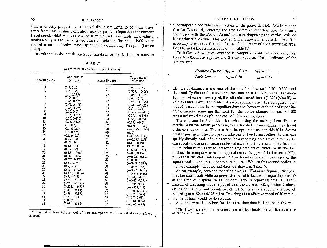
superimpose a coordinate grid system on the police district.t We have done this for District 4, centering the grid system in reporting area 49 (nearly coincident with the Boston Arena) and superimposing the vertical axis on Massachusetts Avenue. This grid system is shown in Figure 2. Then, it is necessary to estimate the coordinates of the center of each reporting area. For District 4 the results are shown in Table IV.

To indicate how travel distance is computed, consider again reporting areas 60 (Kenmore Square) and 2 (Park Square). The coordinates of the centers are:

Kenmore Square: X60 = -0.325

Park Square: Xz = 0.70

Y60 = 0.65

yz = 0.35

The travel distance is the sum of the total "x-distance", 0.70+0.325, and the total "y-distance". 0.65-0.35; the sum equals 1.325 miles. Assuming 10 m.p.h. effective travel speed, the estimated travel time is (1.325) (60)/(10) = 7.95 minutes. Given the center of each reporting area, the computer auto­matically calculates the metropolitan distances between each pair of reporting areas, thereby removing the need for the police planner to specify 4900 estimated travel times (for the case of 70 reporting areas).

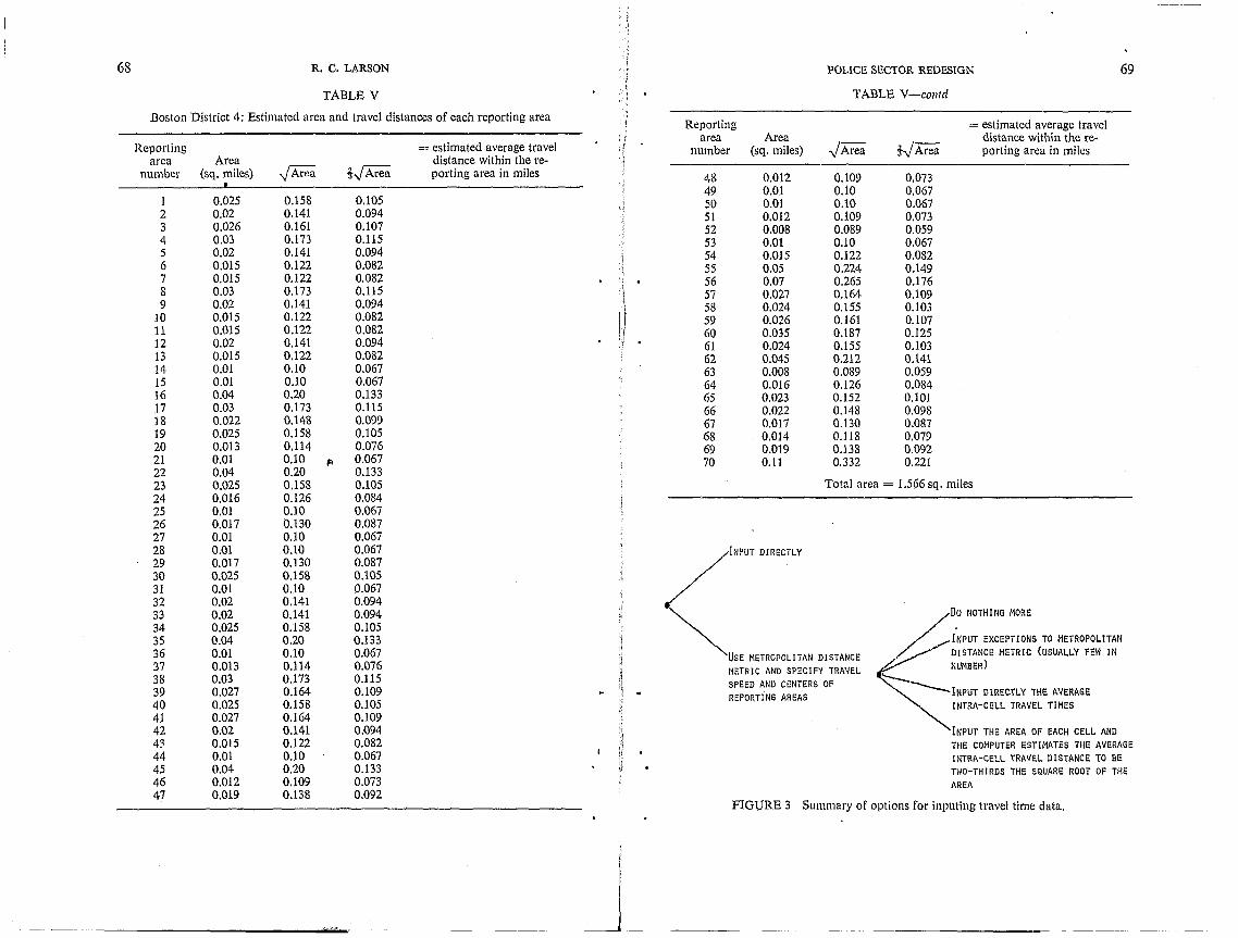
There is one final consideration when using the metropolitan dist:lUce metric. With the above procedure, the estimated intra-reporting area travel distance is zero miles. The user has the option to change this if he desires greater precision. The change can take one of two forms: either the user can specify directly each of the average intra-reporting area travel times or he can specify the area (in square miles) of each reporting area and let the com­puter estimate the average intra-reporting area travel times. With this last option, the computer uses the approximation (suggested in Larson (1972), p. 84) that the mean intra-reporting area travel distance is two-thirds of the square root of the area of the reporting area. We use this second option in the case example. The relevant data are shown in Table V.

As an example, consider reporting area 60 (Kenmore Square). Suppose that the patrol unit while on preventive patrol is located in reporting area 60 at the time of dispatch to an incident, also In reporting area 60. Then,

.. instead o~ assuming that the patrol unit travels zero miles, option 2 above estimates that the unit travels two-thirds of the square root of the area of reporting area 60, or 0.125 miles. Traveling at an effective speed of 10 m.p.h.,

• the travel time would be 45 seconds. A summary of the options for the travel time data is depicted in Figure 3.

t This is 1I0t necessary if all travel times are supplied directly by the police planner or other user of the model.

68 R. C. LARSON POLICE SECTOR REDESIGN 69

TABLE V TABLE V-coll/d

Boston District 4: Estimated area and travel distances of each reporting area Reporting = estimated average travel

area Area t.) Area

distance within the re-Reporting = estimated average travel number (sq. miles) .) Area porting area in miles

area Area distance within the re-number (sq. miles) .J Area i.) Area porting area in miles 48 0.012 0.109 0.073 • 49 om 0.10 0.067

0.025 0.158 0.105 SO 0.01 0.10 0.067 2 0.02 0.141 0.094 5J 0.012 0.109 0.073 3 0.026 0.161 0.107 52 0.008 0.089 0.059 4 0.D3 0.173 0.115 53 0.01 0.10 0.067 5 0.02 0.141 0.094 54 oms 0.122 0.082 6 0,Ol5 0.122 0.082 . 55 0.05 0.224 0.149 7 0.015 0.122 0.082 i

56 0.D7 0.265 0.176 1 . 8 0.03 0.173 0.115 i 57 0.027 0.164 0.109 9 0.02 0.141 0.094

1\ 58 0.024 0.155 0.103

10 0.D15 0.122 0.082 59 0.026 0.161 0.107 11 0.D15 0.122 0.082 J 60 0.035 0.187 0.125 12 0.02 0.141 0.094 I] 61 0.024 0.155 0.103 13 0.015 0.122 0.082 62 0.045 0.212 0.141 14 0.01 0.10 0.067 63 0.008 0.089 0.059 15 0.01 0.10 0.067 64 0.016 0.126 0.084 16 0.Q4 0.20 0.133 65 0.023 0.152 0.101 17 0.D3 0.173 0.115 66 0.022 0.148 0.098 18 0.022 0.148 0.099 67 0.017 0.130 0.087 19 0.025 0.158 0.105 68 0.014 0.118 0.079 20 0.013 0.114 0.076 69 0.019 0.138 0.092 21 0.Q1 0.10 ". 0.067 70 0.11 0.332 0.221 22 0.04 0.20 0.133 23 0.025 0.158 0.105 Total area = 1.566 sq. miles 24 0.016 0.126 0.084 25 0.01 0.10 0.067 26 0.Q17 0.130 0.087 27 0.01 0.10 0.067 28 0.01 0.10 0.067 INPUT DIRECTLY 29 0.017 0.130 0.087 30 0.025 0.158 0.105 31 0.01 0.10 0.067 32 0.02 0.141 0.094

Do NOTHING MORE 33 0.02 0.141 0.094 34 0.025 0.158 0.105 bi"", """"" TO MEm"'LlTA" 35 0.04 0.20 0.133 36 0.01 0.10 0.067 USE METROPOLITAN DISTANCE DISTANCE METRIC (USUALLY FEW IN 37 0.013 0.114 0.076 f1ETRIC AND SPECIFY TRAVEL NUMBER) 38 0.Q3 0.173 0.115 SPEED AND CENTERS OF

---INPUT DIRECTLY THE AVERAGE 39 0.027 0.164 0.109 REPORTI'NG AREAS 40 0.025 0.158 0.105 INTRA-CELL TRAVEL TIMES 41 0.027 0.164 0.109 42 0.02 0.141 0.094 ~ { INPUT THE AREA OF EACH CELL AND 43 0.015 0.122 0.082 H THE COMPUTER ESTIMATES THE AVERAGE 44 0.01 0.10 0.067 'f

Ii INTRA-CELL TRAVEL DISTANCE TO BE 45 0.04 0.20 0.133 i1 TWO-THIRDS THE SQUARE ROOT OF THE 46 0.012 0.109 0.073 AREA 47 0.019 0.138 0.092

FIGURE 3 Summary of options for inputing travel time data.

---------

_J_ ----- ------ ---

70 R. C. LARSON

Preventive patrol coverage

Next it is required to specify how each unit allocates time among its own reporting areas while on preventive patrol. For instance, suppose unit two's sector comprises reporting areas 4, 5, 6, 7, 10 and 11. Then, one must estimate the fraction of the time available for preventive patrol spent in each of these reporting areas. For example, th(~ results of such estimation may be that the unit spends 12.5 per cent of its preventive patrol time in each of the reporting areas 4, 7, 10 and 11, respectively, and 25 percent in each of the remaining two reporting areas (5 and 6).

From the point of view of the sector designer, preventive patrol coverage may be either a controllable 01' an uncontrollable factor in the entire sector design process. If controllable, then when considering a particular design of sectors, the designer must specify not only the overall geometric patterns of sectors (that is, which reporting areas fall into wl1ich sectors), but also how units spend their time when they are in their sectors on preventive patrol. A complete specification ofthe sector plan in this case is a list of which reporting areas fall into which sectors and another list giving the fractions of time each patrol unit spends in each of its reporting areas (while on patrol). Ifpreventive patrol coverage is not controllable by the sector designer, then the fractions of time spent in each reporting area still must be input to the model, but these fractions are prespecified by department rules or by the random behavior of the patrol units (which must be empirically measured).

If the police planner using the model does not specify the preventive patrol coverages, then the model (as a default) assumes that each unit will patrol its reporting areas in direct proportion to the call-for-service volumes from those reporting areas. FOlr instance, again assume that unit two's sector comprises reporting areas 4, 5, 6,7, 10 and 11. From Table II, the call-for­service volumes from these reporting areas are 888, 709, 1666, 1747, 1383 and 1350, respectively. The total call-for-service volume (throughout the sector) is 7743. Thus, the fractions of time spent on preventive patrol in the respective reporting areas are as follows:

Reportir l; Area 4: 888

7743 = 0.115

Reporting Area 5: 709

7743 = 0.092

Reporting Area 6: 1666 7743 = 0.215

Reporting Area 7: 1747 7743 = 0.226

I

, .

POLICE SECTOR REDESIGN

1383 Reporting Area 10: 7743 = 0.179

1350 Reporting Area 11: 7743 = 0.174

71

With such a coverage procedure, reporting area 7, which generates about twice the call~for-service workload of reporting area 4, receives about twice the preventive patrol coverage of reporting area 4.

This default procedure for preventive patrol coverages has an intuitive appeal, in that the more police-related call-for-service activity in a sub·area of a sector, the more likely it is that the sub-area requires preventive patrol attention. However, one must not assume that this default provides for optimal coverage, and ill fact, there are arguments that suggest alternative coverage procedures if one wishes to maximize the probability of intercepting a crime In progress (Larson (1972), pp. 141-148). (In future versions of the model we hope to incorporate an improved default option for preventive patrol coverages that would maximize crime intercept probability.)

To summarize the preventive patrol data requirements, the, planner either supplies the model directly with the fractions of time each unit spends in each of its sectors while on preventive patrol 01' allows the computer to ,assume the default option in which case the preventive patrol coverages within a sector are proportional to call-for-service rates from within the sector.

Average service time

The average service time is defined to be the average of the total "off·the-air" time associated with a call for service. This includes travel time to the scene, on-scene service time, and perhaps off-scene follow-up time spent on report writing, arrest and booking, etc. The workload and queuing characteristics of the system are quite sensitive to the particular numerical value of the ser~ vice time, especially if the system is heavily loaded. Thus, the average service time should be estimated to the nearest minute.

At the time of this writing the best estimate of average service time that we are aware of is based on 1966 data, using a sample of 1788 dispatches. (Larson (1967), p. 169). The average travel time in the District 4 area is approximately 6 minutes and the average on·scene (and off-scene) service time is approximately 32 minutes, yielding 38 minutes as the estimate of the total average service time. In general, other districts in the same city may have different service times.

Dispatcher assignment procedure

The next input data requirement involves the selection procedure used by the dispatcher in assigning units to calls. This is not only important in determining

72 R. C. LARSON

travel time statistics, but it is critically important in determining workloads of the units. In heavy workload situations, in which units may be spending more than half their time servicing calls, units are usually more likely to be assigned by the dispatcher to calls outside their own sector than to calls inside. Thus the amount of intersector or cross-sector dispatching and the manner in which it is directed by the dispatcher play an important role in determining the workload and response time of each unit.

Recalling the "burden of central location", it is possible to have a unit located centrally in a district in a small sector with very little internally generated workload, yet the central location of such a unit could make it an attractive alternative for a cross-sector dispatch to anyone of several sur­rounding sectors. If the frequency of such cross-sector dispatches is high enough for this unit, its workload (as measured by the fraction of time busy servicing calls) could be as high as that of any other unit. Thus the importance of the dispatcher assignment procedure, especially for cross-sector assign­ments.

The model assumes that the dispatcher has a rank ordering of preferred patrol units to dispatch to each reporting area. Forinstance, consider reporting area 7 and suppose there are six patrol units assigned to District 4, numbered consecutively from one to six. Then, the dispatcher probably first prefers the unit whose sector includes reporting area 7. Say that reporting area 7 is contained in sector 1; then unit 1 would be the first preferred. If sector 3 and sector 4 both touch sector 1, then the dispatcher is likely to prefer units 3 and 4 (or perhaps 4 and 3, respectively) as the second and third choices. The entire rank ordering may look something like this for reporting area 7: unit 1, 3, 4, 2, 6, 5. Then, when a call for service occurs from reporting area 7, the dispatcher always assigns the most preferred available unit. For example, ifunits 1, 3 and 6 are unavailable when a call is rep<?rted from reporting area 7, then the dispatcher assigns unit 4 to the call; unit 4 is the most preferred of the available units (which are units 2, 4 and 5).

This ranking scheme has sufficient flexibility to model many different police department operations. For instance, suppose that six regular sector cars and two patrol supervisor cars are fielded on a particular tour in District 4. t Given a call for service, the dispatcher may assign the sector car estimated to be the closest available, if at least one of the six is available; if not, he may select the closest available patrol supervisor car; if all eight cars are busy, he would delay the call in queue. In such a situation the rank orderings of the dispatcher would always place the two patrol supervisor cars at the end of the

t The computer model allows any degree of overlapping sectors. Thus, for instance, one could use the model to study the operational performance of a system with six regular sector units (assigned to nonoverlapping sectors) and two patrol supervIsor cars (each assigned to patrol and supervise three of the regular sectors).

POLlCE SECTOR REDESIGN 73

preference list (in slots seven and eight); entries in slots one through six would be determined by estimated travel times of the six sector cars.

As another example, it may be determined that the officers in a particular car are especially competent in servicing the calls from one particular neighborhood. For instance, in a Spanish-speaking neighborhood one would like to assign officers who are fluent in both English and Spanish. Such a preference for particular officers is likely to override concern for minimizing travel time, at least as long as travel time is kept within some reasonable limit. The police planner can model this situation by making the "Spanish­speaking car" first preference for all reporting areas within the command that have a large Spanish-speaking population, regardless of sector boun­daries that dictate where the unit performs preventive patrol and regardless of the fact that other units may be closer (in a travel time sense) to some or all of the Spanish-speaking neighborhoods.

Specifying the dispatcher preferences for each reporting area in a command often requires providing the model with a large set of numbers. In a case with 70 reporting areas and six patrol units, 6 x 70 = 420 numbers (preferences) are required. To help alleviate this burden the model has preprogrammed eight different dispatching strategies that fairly accurately depict the general types of dispatcher decision-making that are found in police departments through­out the United States. These eight are all based on geographical considera­tions and do not provide the richness in dispatching strategies that is allowed if one generates the dispatcher preferences directly. In using the model, however, the police planner can use a mixture of strategies by selecting one of the eight geographically-based strategies and then overriding that strategy for particular units and/or particular reporting areas. For instance, in the case of six regular sector units and two patrol supervisor units, the police planner could select geographically-based strategy number 3, but dictate to the model that units 7 and 8 (the patrol supervisors) are always to be given last preference, regardless of geographical considerations.

The eight geographically-based strategies fall into two groups: strategies 1 through 4 always give first preference to the sector car, while strategies 5 ': through 8 do not. Except for that qualification, strategies 1 and 5 are identical, . as are 2 and 6, 3 and 7, and 4 and 8. The differences among strategies 1 through 4 (and 5 through 8) depend on how accurately the dispatcher esti­mates travel distance from each unit's sector to each reporting area. At the crudest level, strategy 1 assumes that the dispatcher acts as if (1) each available unit were at the statistical center (based on relative allocations of preventive patrol effort) of its respective sector and (2) each call for service were at the statistical center (based on call-for-service data) of the patrol sector con­taining the call for service. Such a strategy generates the same list of dispatch preferences for every reporting ar.:a within the same sector. However crude

74 R. C. LARSON

this procedure is, the author has found it to be a fairly accurate model of the dispatching strategies of many different dispatchers.

At the other extreme, strategy number 4 assumes that the dispatcher uses in the best way possible all the information he has regarding the location of the call for service and its relationship to the statistical locations of all units. (It does not assume, however, that the dispatcher knows the exact location of any of the patrolling cars.)

Strategies 2 and 3 might be considered "intermediate" between strategies 1 and 4. The technical details of the strategies are discussed elsewheret and need not concern us here.

For ease in presentation of the case example, we assume that the dispatcher uses strategy 1 in which travel distance estimates are based on the assumption that both the patrol unit and the call for service are located at the statistical centers of their respective sectors. In the case study we assume that preventive patrol effort in a particular reporting area in a sector is proportional to the call-for-service rate from that reporting area. Thus, the distribution over reporting areas of calls for service and preventive patrol are identical. In such a situation the statistical center of a sector for the patrol unit is identica) to the statistical center of the sector for the call for service (since both are identically distributed over the reporting areas of the sector).

To provide an example, suppose the statistical centers of sectors 1 and 2 were as follows:

Sector 1: Xl = 0 mile

Sector 2: X2 = 1.5 miles Yl = 0 mile

Y2 = 0.5 mile

Then, when deciding dispatch preferences, the dispatcher would estimate that any call for service from sector 1 was located at its center (Xl = 0 and y 1 = 0) and any call from sector 2 was located at its center (X2 = 1.5 and Y2 = 0.5); similarly, the dispatcher wou.ld act as if the sector 1 car, while on patrol, was located at its center (Xl = 0, Yl = 0) and the sector 2 car, while on patrol, was at its center (X2 = 1.5, Y2 = 0.5). Then the estimated travel distance for the sector 1 car to reach a sector 1 call would be (0 - 0) + (0 - 0) = o miles (and similarly for the sector 2 car to each a sector 2 call). The estimated travel distance for the sector 1 car to reach a sector 2 call would be (1.5 - 0) + (0.5 - 0) = 2 miles (and similarly for the sector 2 car to reach a sector 1 call). Thus the sector 1 car would always be preferred to the sector 2 car for any cali from sector 1 (and vice versa for a call from sector 2).

Although these dispatch preferences are based on only crude estimates of travel times, the model subsequently computes the statistically exact average travel times (given the input data) that result from using the dispatching strategy. Thus, if a dispatching selection is made that estimates a mean travel

t Larson (1972), pp. 85-100.

POLICE SECTOR REDESIGN 75

time of 1 minUte but the true mean travel time is 2 minutes, the computed outputs correctly incorporate the latter 2-minute figure.

We have now completed all but one of the data requirements for the model and this follows.

The total number of units

We still need to specify how many units will be fielded in the district. Should a particular time period have four units, six, ten, or IS? The answer to that ~ue.stion . d~~en~s on. many factors, including legal constraints which may lImIt flexlbllIty m assIgnment procedures. One of the key operational factors that influences' the total number of units required is the anticipated number of calls for service to be received per hour during the tour. If one has an esti­mat~ of th!s call-for-service rate and of the average service time, then by relatIvely SImple global models-r the police planner can predict the overall average car workloads and congestion level of the district for each alternative number of cars that may be fielded. Thus, for instance, the police planner may ~tate his global planning objective in the following way: "I wish to assign suffiCIently many units to this time period so that at least 90 percent of all calls for service are assigned to cars without any dispatching delay." The "90 per.cent" may be changed to another value, say 80 percent or 95 percent, dependmg on departmental policy.

In this case example we assume that the police planner, using past statistics of calls for service, estimates that an average of 4.737 calls for service will be generated per hour during the period of interest. Given 4.737 calls per hour and 38 minutes average service time per call, he finds that six units nt!ed to be fielded during the period in order to assume that 90 percent will be handled without dispatch delay. This calculation is made using a simple queuing formula that is widely available (and suitable for calculation with an electronic calculator)·t

Since an average of 4.737 calls are generated each hour and since each requires an average of 38 minutes to service, we have 38 x 4.737 = 180 minutes of call-for-service workload each hour. If six units are allocated, then the average wo~kload per unit is

180 minutes of workload per hour (6 units) = 30 minutes per hour per unit.

Thus, on the average, units will be busy servicing calls 50 percent of the time. In District 4, four to five calls per hour is a below-average call-for-service

workload that may correspond to such periods as 12.0; a.m. to 3.00 a.m.

t See, for example, Chaiken and Larson (1972). + See Larson (1972), Chapter 5.

76 R. C. LARSON

(weekdays) or 6.00 a.m. to 11.00 a.m. (weekdays) or all day Sunday. Assum­ing sectors that vary by time of day, other heavier workload periods would require a greater number of units and thus a greater number of sectors.

SECTOR REDESIGN PROCESS

We are now confronted with the task of partitioning District 4 in Boston into six patrol sectors. Our data assumpti.ons are briefly summarized as follows:

1) The district is partitioned into 70 reporting areas, numbered consecu­tively from 1 to 70, as shown in Figure 2. Each sector to be designed must be made up of one or more entire reporting areas; no reporting area is to be split in two. Sectors are to be nonoverlapping. Each reporting area must be part of a sector.

2) O..1ls for service are distributed among reporting areas as shown in Table II.

3) Travel times are assumed to be proportional to travel distances, which are assumed to be based on the "Manhattan" distance metric. Effective trave~ speed is assumed to be 10 m.p.h.

4) The fraction of the available preventive patrol coverage in a sector given to a particular reporting area is assumed to be proportional to the call­for-service volume (workload) from that reporting area.

5) The average service time (travel time plus on-scene and perhaps off­scene follow-up time) is assumed to be 38 minutes.

6) The dispatcher, in his assignment procedure, always gives first prefer­ence to the sector car. If the sector car is not available, he assigns the out-of­sector car estimated to be closest to the call; he estimates travel distance (and consequently travel time) by assuming that both patrol units and caUs for service are at the statistical\. 'nters of their respective sectors.

7) There are six total units to be fielded, and thus six sectors to be designed.

8) An average of 4.737 calls for service arrive per hour from District 4. Units are busy servicing calls an average of 50 percent of the time.

Iteration number 1 : A rough cut at equal sector workloads

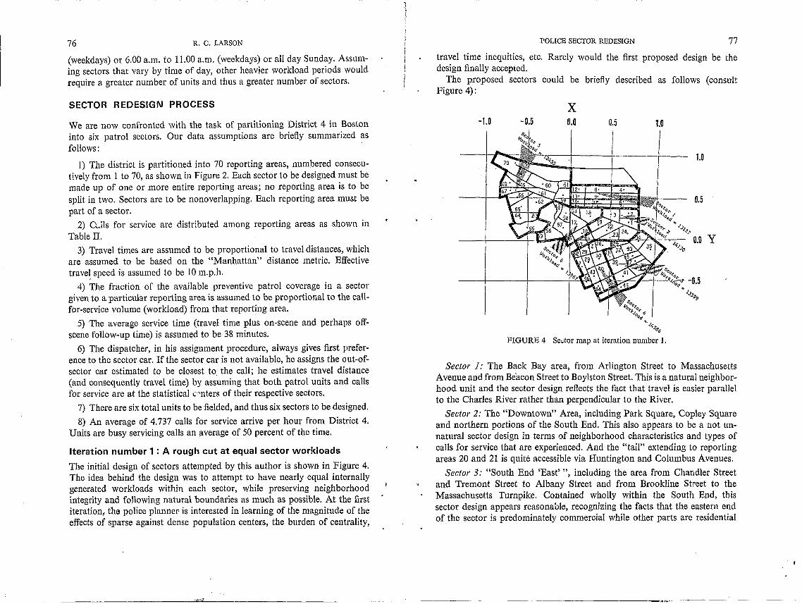
The initial design of sectors attempted by this author is shown in Figure 4. The idea behind the design was to attempt to have nearly equal internally generated workloads within each sector, while preserving neighborhood integrity and following natural boundaries as much as possible. At the first iteration, the police planner is interested in learning of the magnitude of the effects of sparse against dense population centers, the burden of centrality,

POLlCE SECTOR REDESIGN 77

travel time inequities, etc. Rarely would the first proposed design be the design finally accepted.

The proposed sectors could be briefly described as follows (consult Figure 4):

-1.0 -0.5 x 0.0 0.5 1.0

~IS'~~ Ol-oft-ot-

lo~/

~'./"s. O'.s-

FIGURE 4 Se ... tor map at iteration number 1.

1.0

0.5

y

Sector '1: The Back Bay area, from Arlington Street to Massachusetts Avenue and from Be'acon Street to Boylston Street. This is a natural neighbor­hood unit and the sector design reflects the fact that travel is easier parallel to the Charles River rather than perpendicular to the River.

Sector 2: The "Downtown" Area, including Park Square, Copley Square and northern portions of the South End. This also appears to be a not un­natural sector design in terms of neighborhood characteristics and types of calls for service that are experienced. And the "tail" extending to reporting areas 20 and 21 is quite accessible via Huntington and Columbus Avenues.

Sector 3: "South End 'East' ", including the area from Chandler Street and Tremont Street to Albany Street and from Brookline Street to the Massachusetts Turnpike. Contained wholly within the South End, this sector design appears reasonable, recognizing the facts that the eastern end of the sector is predominately commercial while other parts are residential

78 R. C. LARSON

and still others contain shops, bars and entertainment areas. Except for the inclusion of the elongated reporting area 45 (Albany Street), the sector geometry reflects a compact design, thereby keeping average intrasector travel time near the minimum possible value.

Sector 4: "South End 'West' ", including the area from Columbus Avenue and Warren Avenue to Albany Street and from Camden Street and Lenox Street to Brookline Street. This sector also has a "neighborhood" orientation and a compact design.

Sector 5: "Kenmore Square-Fenway Park", including the area west from Massachusetts Avenue and south from the River to the Park Drive area. This is one of the most troublesome areas for which to design an appropriate sector due to the diversity of the neighborhoods within the area and due to the relatively lighter workload per square mile in the area. The latter concern plus the area's relative remoteness from the remainder of District 4 will result in relatively large travel times in the area.

Sector 6: "Fens-Prudential Cel!ter", including the area from the Fenway to Copley Square and from Boylston Street to Columbus Avenue. This sector is perhaps least satisfactory from a "neighborhood" point of view, containing almost every type of neighborhood that is found in District 4. It is centrally located and relatively compact.

The estimated operating performance of District 4 with the proposed sector design is shown in Tables VI and VII. All of the numbers in these tables were generated from the computer model, under the assumptions discussed earlier. We now examine the entries in the tables to illustrate their meaning in the context of the District 4 example:

Maximum workload imbalance = 26% This means that if we subtract the workload of the least busy unit from the workload of the busiest unit, divide by the district-wide average workload, and multiply by 100 percent, we get the maximum workload imbalance of 26 percent. Note that the busiest unit is unit 2 (the "downtown unit"), which works 11.7 percent above the average, and the least busy unit is unit 5 (the Kenmore Squf\.re-Fenway Park unit), which works 14.3 percent below the average. As another measure of maximum workload imbalance, we could calculate that the busiest unit works 30 percent "harder" than the least busy unit.

Region-wide average travel time = 3.402 minutes

This means that the average travel time to calls in District 4, averaged over all call locations and all levels of patrol force saturation or nonsaturation, is 3.402 minutes. The four significant figures are retained not to support a claim of model precision (when compared to actual District 4 operations), but to

POLICE SECTOR REDESIGN 79

spot upward or downward shifts in travel time with alternative sector desi~ns. in subsequent ite:ations. (A similar comment applies to all other entnes 111 the table for whlCh more than two significant figures are retained.)

Average travel time for queued calls = 5.178 minutes

Assuming that queued. calls are handled in a first-in, first-out manner, this ~ays tha~ the average travel time required to reach a call that has been delayed 111 the dIspatcher queue (due to car unavailabilities) is 5.178 minutes.

Fraction of dispatches that are cross-sector = 0.485

Th.is means that ~8.5 percent of all dispatch assignments require sending a umt to a call outSIde of the unit's own sector.

The next part of the table provides a breakout of operating characteristics by patrol unit number. To interpret an example, patrol unit 2 spends 55.9 percent of its time servicing calls; this is 11.7 percent above the average workload; 57.6 percent of its assignments take it outside of sector 2 and this is 18.7 percent above the average amount of cross-secto, assignm;nts; and

Patrol unit no.

1 2 3 4 5 6

Sector no.

1 2 3 4 5 6

TABLE VI

Maximum workload imbalance = 26 % Region-wide average travel time = 3.402 minutes Average travel time for queued calls = 5.178 minutes Fraction of dispatches that are cross-sector = 0.485

Profile of patrol unit operations

%of Fraction of dispatches % of Workload mean out of sector mean

0.519 103.8 0.539 111.3 0.559 .111.7 0.576 118.7 0.496 99.2 0.477 98.5 0.490 98.0 0.426 87.9 0.428 85.7 0.373 no 0.507 101.5 0.487 100.4

Profile of sector operations

Fraction of district's % of Fraction of dispatches total workload mean that are cross-sector

0.160 96.2 0.503 0.172 103.6 0.542 0.166 99.7 0.480 0.178 106.9 0.474 0.152 91.3 0.412 0.170 102.4 0.491

Iteration #1

Average travel time

3.432 3.378 3.090 3.180 3.978 3.414

Average travel time

3.312 3.120 3.324 3.258 4.218 3.258

80 R. C. LARSON

unit 2 requires an average of 3.378 minutes to reach the scene of a caIl to which it is dispatched.

The final part of the table provides a breakdown by sector. Looking at sector 2, we note that it generates 17.2 percent of the district's total workload, and this is 3.6 percent above the mean; 54.2 percent of caIls for service from sector 2 require a unit other than unit 2 to respond to the call; and the average travel time to a sector 2 call for service is 3.120 minutes.

The second table (Table VII) provides a breakdown for selected reporting areas. (The model calculates similar figures for all 70 reporting areas, but these figures are too numerous to report here.) As an example, reporting area 16 (Prudential Center) generates an average of 8.3 calls per 100 hours; it experiences an average travel time delay of 3.078 minutes and 12 percent of its calls are handled by unit 1, 19 percent by unit 2, 4 percent by unit 3, 5 percent by unit 4, 9 percent by unit 5, and 51 percent by unit 6, the unit whose sector includes the Prudential Center.

TABLE VII Iteration #1

Profile of selected reporting areas

Fraction of calls handled by unit: Calls! Average 100 travel 2 3 4 5 6

hours time

ReporUng area 2: 12.8 3.204 0.23 0.46 0.14 0.05 0.04 0,07 Park Square

Reporting area 16: Prudential Center 8.3 3.078 0.12 0.19 0.04 0.05 0.09 0.51

Reporting area 26: Warren and Columbus Aves. 8.6 2.928 0.04 0.10 0.21 0.53 0.04 0.08

Reporting area 39: Washington St. and Union Park 11.8 3.006 0,07 0.10 0.52 0.21 0.04 0.05

Reporting area 45 : Albany St. 4.3 4.158 0,07 0.10 0.52 0.21 0.04 0.05

Reporting area 57: Hemenway St. to Mass. Ave. 15.6 3.108 0.12 0.19 0.04 0.05 0.09 0.51

Reporting area 60: Kenmore Square 10.5 3.924 0.09 0.05 0.04 0.05 0.59 0.18

Reporting area 68: Beacon St. and Park Drive 6.7 4.938 0.09 0.05 0.04 0.05 0.59 0.18

The author spent about 30 to 45 minutes studying the results in these two tables and interpreting them in terms of the sector map (Figure 4). Playing the role of police planner, he decided that the workload imbalance was too

POLICE SECTOR REDESIGN 81

great, so he tried to devise an alternative sector map to reduce workload imbalance.

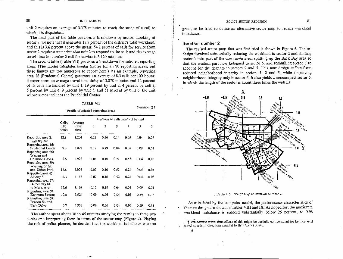
Iteration number 2 The revised sector J,11ap that was first tried is shown in Figure 5. The re­

design involved substantially reducing the workload in sector 2 and shifting sector 1 into part of the downtown area, splitting up the Back Bay area so that the western part now belonged to sector 5, and reshuffiing sector 6 to account for the changes in sectors 2 and 5. This new design suffers from reduced neighborhood integrity in sectors 1, 2 and 5, while improving neighborhood integrity only in sector 6. It also yields a noncompact sector 5, in which the length of the sector is about three times the width. t

x

FIGURE 5 Sector map at iteration number 2.

As calculated by the computer model, the performance characteristics of the new design are shown in Tables VIII and IX. As hoped for, the maximum workload imbalance is reduced substantially below 26 percent, to 9.98

t The adverse travel time effects of this might be partially compensated for by increased travel speeds in directions parallel to the Charles RIver.

6

82 R. C. LARSON

percent. However, unit 2 is still the busiest unit (5.5 percent above average) and unit 5 is still the least busy unit (4.6 percent below average). The reduc­tion in workload imbalances also caused a very slight reduction in the amount of cross-section dispatching. The district-wide av.erage travel time increased slightly to 3.456 minutes (an increase of about 1.3 percent). Mbredisturbing are the approximately 10 percent increases in travel times in sectors 5 and 6, due primarily to the revised geometries and the increased workload of unit 5. The average travel time to reporting area 68 (Beacon Street and Park Drive) is increased from 4.938 minutes to 5.676 minutes (an increase of 15 percent).

Patrol unit no.

1 2 3 4 5 6

Sector no.

J 2 3 4 5 6

TABLE VIII

Maximum workload imbalance = 9.98 % Region-wide average travel time = 3.456 minutes Average travel time for queued calls = 5.178 minutes Fraction of dispatches that are cross-sector = 0.483

Profile of patrol unit operations

% of Fraction of dispatches % of Workload mean out of sector mean

0.509 101.9 0.516 106.8 0.527 105.5 0.563 116.5 0.501 100.1 0.486 100.7 0.504 100.8 0.457 94.5 0.477 95.5 0.426 88.3 0.481 96.2 0.441 91.3

Profile of sector operations

Fraction of district's % of Fraction of dispatches total workload mean that are cross-sector

0.162 97.3 0.493 0.157 94.2 0.511 0.166 99.7 0.484 0.178 106.9 0.488 0.169 101.6 0.461 0.167 100.4 0.465

Iteration #2

Average travel time

3.246 3.360 3.210 3.168 4.164 3.636

Average travel time

3.018 3.066 3.318 3.258 4.422 3.612

The police planner must study these figures, weigh the importance of balanced workloads against that of police accessibility to various neighbor­hoods and other factors, and he must decide to alter the sector map still further, to accept the currently proposed sector map, or to retrace steps and accept a previously examined sector map.

Playing the role of police planner here, this author decided to pursue the balancing of workloads, in effect discounting the importance of police

POLICE SECTOR REDESIGN 83

accessibility as measured by travel times. It must be emphasized that this is a purely arbitrary choice that may not reflect the priorities of many police

planners.

TABLE IX Iteration #2

Profile of selected reporting areas

Calls! Average Fraction of calls handled by unit: 100 travel hours time 2 3 4 5 6

Reporting area 2 : Park Square 12.8 2.g:28 0.51 0.20 0.13 0,03 0.09 0.05

Reporting area 16: Prudential Center 8.3 3.108 0.22 0.49 0.07 0.13 0.04 0.06

Reporting area 26: Warren and Columbus Aves. 8.6 2.898 0.07 0.11 0.21 0.51 0.04 0.06

Reporting area 39: Washington St.

0.52 0.21 0.04 0.06 and Union Park 11.8 3.150 0.07 0.11 Reporting area 45 :

0.11 0.52 0.21 0.04 0.06 Albany St. 4.3- 4.164 0.07 Reporting area 57:

Hemenway St. to Mass. Ave. 15.6 3.138 0.06 0.11 0,03 0.05 0.21 0.54

Reporting area 60: Kenmore Square 10.5 4.260 0.11 0.06 0,03 0.05 0.54 0.21

Reporting area 68: Beacon St. and Park Drive 6.7 5.676 0.11 0.06 0.03 0.05 0.54 0.21

Iteration number3: Interchanging St. Cecilia Street reporting area

Examining the performance of the district with the sector map of iteration number 2, this planner initially felt that removing just one reporting area from sector 2 could reduce the workload of patrol unit two to near normal. Since sectors 3 and 4 scored high on the "neighborhood integrity" scale and since their units had almost exactly average workloads, it was decided to leave sectors 3 and 4 intact. The workload of unit 1 was also very close to average, so sector one was left intact. The only viable option was to reassign reporting area 53, centering on St. Cecilia Street, to either sector 5 or sector 6. Even though sector 5 would be the obvious choice on grounds of workload balancing, it was ruled out on grounds of neighborhood integrity and resulting noncompact sector geometry. Thus reporting area 53 was assigned to sector 6, in the hope that the workload of unit 6 would increase above the 96.2 mark; it was also hoped that the workload of unit 5 would increase above the

~-------------------------,-.,------

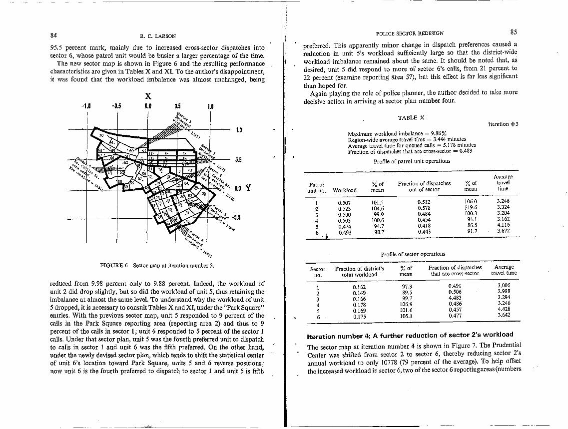
84 R. C. LARSON

95.5 percent mark, mainly due to increased cross-sector dispatches into sector 6, whose patrol unit would be busier a larger percentage of the time.

The new sector map is shown in Figure 6 and the resulting performance characteristics are given in Tables X and XI. To the author's disappointment, it was found that the workload imbalance was almost unchanged, being

-0.5 X 0.0 0.5 1.0

FIGURE 6 Sector map at iterlltion number 3.

reduced from 9.98 percent only to 9.88 percent. Indeed, the workload of unit 2 did drop slightly, but so did the workload of unit 5, thus retaining the imbalance at almost the same level. To understand why the workload of unit 5 dropped, it is necessary to consult Tables X and XI, under the "Park Square" entries. With the previous sector map, unit 5 responded to 9 percent of the calls in the Park Square reporting area (reporting area 2) and thus to 9 perct~nt of the calls in sector 1; unit 6 responded to 5 percent of the sector 1 calls. Under that sector plan, unit 5 was the fourth preferred unit to dispatch to calls in sector 1 and unit 6 was the fifth rreferred. On the other hand, under the newly devised sector plan, which tends to shift the statistical center -of unit 6's location toward Park Square, units 5 and 6 reverse positions; now unit 6 is the fourth preferred to dispatch to sector 1 and unit 5 is fifth

POLICE SECTOR REDESIGN 85

preferred. This apparently minor change in dispatch preferences caused a reduction in unit 5's workload sufficiently large so that the district-wide workload imbalance remained about the same. It should be noted that, as desired, unit 5 did respond to more of sector 6's calls, from 21 percent to 22 percent (examine reporting area 57), but this effect is far less significant than hoped for.

Again playing the role of police planner, the author decided to take more decisive action in arriving at sector plan number four.

Patrol unit no.

1 2 3 4 5 6

"

Sector no.

1 2 3 4 5 6

TABLE X

Maximum workload imbalance = 9.88% Region-wide average travel time = 3.444 minutes Average travel time for queued calls = 5.178 minutes Fraction of dispatches that are cross-sector = 0.483

Profile of patrol unit operations

% of Fraction of dispatches % of Workload mean out of sector mean

0.507 101.5 0.512 106.0 0.523 104.6 0.578 119.6 0.500 99.9 0.484 100.3 0.503 100,6 0.454 94.1 0.474 94.7 0.4J8 86.5 0.493 98.7 0.443 91.7

Profile of sector operations

Fraction of district's % of Fraction of dispatches total workload mean that are cross-sector

0.162 97.3 0.491 0.149 89.5 0.506 0.166 99.7 4.483 1,).178 106.9 0.486 0.169 101.6 0.457 0.175 105.1 0.477

Iteration #3

Average travel time

3.246 3.324 3.204 3.162 4.116 3.672

Average travel time

3.006 2.988 3.294 3.246 4.428 3.642

Iteration number tl: A further reduction of sector 2's workload

The sector map at ite\\'ation number 4 is shown in Figure 7. The Prudential Center was shifted frli)m sector 2 to sector 6, thereby reducing sector 2's annual workload to only 10778 (79 percent of the average). To help offset the increased workload in sector 6, two of the sector 6 reporting areas (numbers

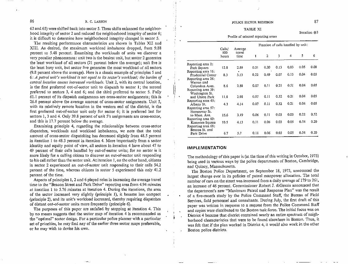
86 R. C. LARSON

62 and 65) were shifted back into sector 5. These shifts enhanced the neighbor­hood integrity of sector 2 and reduced the neighborhood integrity of sector 6; it is difficult to determine how neighborhood integrity changed in sector 5.

The resulting performance characteristics are shown in Tables XII and XIII. As desired, the maximum workload imbalance dropped, from 9.88 percent to 5.48 percent. Examining the workloads of units we discover a very peculiar phenomenon: unit two is the busiest unit, but sector 2 generates the least workload of all sectors (21 percent below the average); unit five is the least busy unit, but sector five generates the most workload ur all sectors (9.8 percent above the average). Here is a classic example of principles 5 and 6: A patrol unit's workload is not equal to its sector's workload; the burden of central location causes increased workloads. Unit 2, with its central location, is the first preferred out-of-sector unit to dispatch to sector 1; the second preferred to sectors 3, 4 and 6; and the third preferred to sector 5. Fully 61.1 percent of its dispatch assignments are cross-sector assignments; this is 26.6 percent above the average amount of cross-sector assignments. Unit 5, with its relatively remote location in the western end of the district, is the first preferred out-of-sector unit only for sector 6; it is preferred last for sectors 1,3 and 4. Only 39.8 percent of unit 5's assignments are cross-sector, and this is 17.7 percent below the average.

Examining principle 4, regarding the relationships between cross-sector dispatches, workloads and workload imbalances, we note that the total amount of cross-sector dispatching has decreased slightly from 48.5 percent in iteration 1 to 48.3 percent in iteration 4. More importantly from a sector identity and equity point of view, all sectors in iteration 4 have about 47 to 49 percent of their calls handled by out-of-sector units; for no sector is it more likely for 11 calling citizen to discover an out-of-sector unit responding to his call rather than the sector unit. At iteration 1, on the other hand, citizens in sector 2 experienced an out-of-sector unit responding to their caIls 54.2 percent of the time, whereas citizens in sector 5 experienced this only 41.2 percent of the time.

Aspects of principles 1,2 and 6 played roles in increasing the average travel time to the "Beacon Street and Park Drive" reporting area from 4.94 minutes at iteration 1 to 5.76 minutes at iteration 4. During the iterations, the area of the sector increased very slightly (principle 1), it became less compact (principle 2), and its unit's workload increased, thereby requiring dispatches of distant out-of-sector units more frequently (principle 6).

The purposes of this paper are satisfied by stopping at iteration 4. This by no means suggests that the sector map of iteration 4 is recommended as the "optimal" sector design. For a particular police planner with a particular set of priorities, he may find any of the earlier three sector maps preferrable, or he may wish to devise his own.

POLICE SECTOR REDESIGN 87

TABLE XI Iteration #3

Profile of selected reporting areas

Fraction of caBs handled by unit: Calls! Average

100 travel hours time 1 2 3 4 5 6

Reporting area 2: Park Square 12.8 2.89 0.5\ 0.20 0.13 0.03 0.05 0.08

Reporting area 16: Prudential Center 8.3 3.13 0.22 0.49 0.07 0.13 0.04 0.05

Reporting area 26: Warren and Columbus Aves. 8.6 2.88 0.07 0.11 0.21 0.51 0.04 0.05

Reporting area 39: Washington SI. and Union Park 11.8 2.98 0.Q7 O.ll 0.52 0.21 0.04 0.05

Reporting area 45: Albany SI. 4.3 4.14 0.07 0.11 0.52 0.21 0.04 0.05

Reporting area 57: Hemenway St. to Mass. Ave. 15.6 3.19 0.06 0.11 0.03 0.05 0.22 0.52

Reporting area 60: Kenmore Square 10.5 4.13 0.11 0.06 0.03 0.05 0.54 0.20

Reporting area 68: Beacon SI. and Park Drive 6.7 5.7 0.11 0.06 0.03 0.05 0.54 0.20

IMPLEMENTATION

The methodology of this paper is (at the time of this writing in October, 1973) being used in various ways by the police departments of Boston, Cambridge, and Quincy, Massachusetts.

The Boston Police Department, on September 18, 1973, announced the largest change ever in its policies of patrol manpower allocation. The total number of cars on the street was increased from a daily average of 179 to 261, an increase of 46 percent. Commissioner Robert J. diGrazia announced that the department's new "Maximum Patrol and Response Plan" was the re~ult of a five-month study by the Police Command Staff, t.he Bureau of FIeld Services, field personnel and consultants. During July, the first draft of this paper was written in response to a request from the Poli.ce. ~ommand Staff and copies were distributed to the Boston task force. The Huhal focus wa~ on District 4 because that district contained nearly an entire spectrum of neIgh­borhood characteristics that were to be found elsewhere in Boston. TllUs, it was felt that if the plan worked in District 4, it would also work in the other Boston police districts.

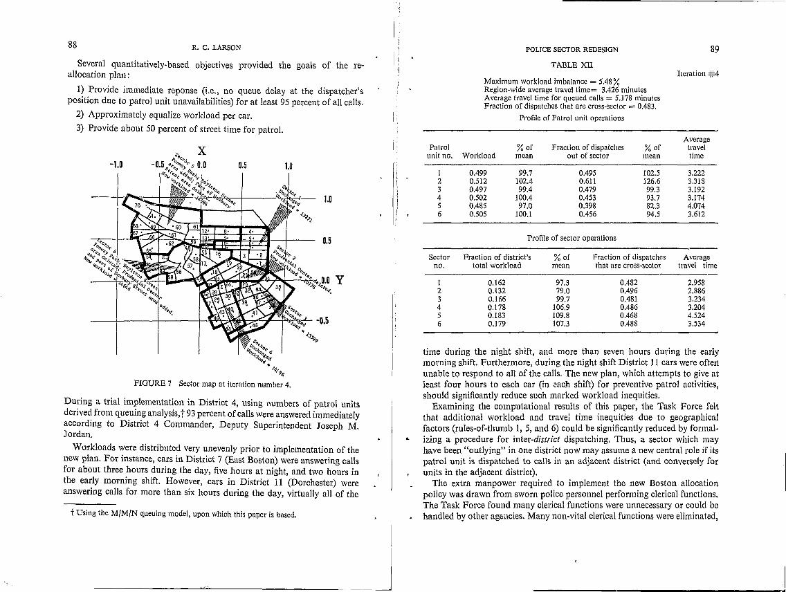
88 R. C. LARSON

Several quantitatively-based objectives provided the goals of the re­allocation plan:

1) Provide immediate reponse (i.e., no queue delay at the dispatcher's position due to patrol unit unavailabilities) for at least 95 percent of all calls.

2) Approximately equalize workload per car.

3) Provide about 50 percent of street time for patrol.

y

FIGURE 7 Sector map at iter,ation number 4.

During a trial implementation in District 4, using numbers of patrol units derived from queuing analysis, t 93 percent of calls were answered immediately according to District 4 Commander, Deputy Superintendent Joseph M. Jordan.

Workloads were distributed very unevenly prior to implementation of the new plan. For instance, cars in District 7 (East Boston) were answering calls for about three hours during the day, five hours at night, and two hours in the early morning shift. However, cars in District 11 (Dorchester) were answering calls for more than six hours during the day, virtually all of the

t Using the M/M/N queuing model, upon which this paper is based.

i -,;

;

I'

i,

Patrol unit no.

2 3 4 5 6

Sector no.

1 2 3 4 5 6

POLlCE SECTOR REDESIGN

TABLE XU

Maximum workload imbalance = 5.48 % Region-wide average travel time= 3.426 minutes Average travel time for queued caBs = 5.178 minutes Fraction of dispatches that are cross-sector = 0.483.

Profile of Patrol unit operations

% of Fraction of dispatches % of Workload mean out of sector mean

0.499 99.7 0.495 102.5 0.512 102.4 0.611 126.6 0.497 99.4 0.479 99.3 0.502 100,4 0.453 93.7 0.485 97.0 0.398 82.3 0.505 100.1 0.456 94.5

Profile of sector operations

Fraction of district's % of Fraction of dispatches total workload mean that are cross-seclor

0.162 97.3 0.482 0.132 79.0 0.496 0.166 99.7 0.481 0.178 106.9 0.486 0.183 109.8 0.468 0.179 107.3 0.488

89

Iteration #4

Average travel time

3.222 3.318 3.192 3.174 4.074 3.612

Average travel time

2.958 2.886 3.234 3.204 4.524 3.534

time during the night shift, and more than seven hours during the early morning shift. Furthermore, during the night shift District 11 cars were often unable to respond to aU of the calls. The new plan, which attempts to give at least four hours to each car (in ~ach shift) for preventive patrol activities, should significantly reduce such marked workload inequities.

Examining the computational results of this paper, the Task Force felt that additional workload and travel time inequities due to geographical factors (rules-of-thumb 1, 5, and 6) could be significantly reduced by formal-

.. izing a procedure for inter-district dispatching. Thus, a sector which may have been "outlying" in one district now may assume a new central role if its patrol unit is dispatched to calls in an adjacent district (and conversely for units in the adjacent district).

The extra manpower required to implement the new Boston allocation policy was drawn from sworn police personnel performing clerical functions. The Task Force found many clerical functions were unnecessary or could be handled by other agencies. Many non-vital clerical functions were eliminated,

90 R. C. LARSON

TABLE XIII Iteration #4

Profile of selected reporting areas

Calls/ Average 100 travel

hOllrs time 2 3 4 S 6

Reporting area 2: Park Square 12.8 2.82 0.S2 0.20 0.13 0.04 0.04 0,07

Reporting area 16: 0.05 Prudential Center 8.3 3.47 0,07 0.12 0.D3 0.22 O.Sl

Reporting area 26: Warren and Columbus Aves. 8.6 2.87 0.04 0.11 0.21 0.51 0.04 0.08

Reporting area 39: Washington St. and Union Park 11.8 2.92 0.07 0.11 0.S2 0.21 0.04 O.OS

Reporting area 45: Albany St. 4.3 4.08 0.D7 0.11 0.52 0.21 0.04 0.05

Reporting area S7: Hemenway St. to Mass. Ave. lS.6 3.16 0.Q7 0.12 0.03 O.OS 0.22 0.51

Reporting area 60: Kenmore Square 10.5 4.34 0.12 0.06 0.D3 0.05 0.S3 0.20

Reporting area 68: Beacon St. and Park Drive 6.7 S.76 0.12 0.06 0.03 O.OS 0.S3 0.20

including such functions as duplicating records at the district level that were available at headquarters. New organizations were drawn for district per­sonnel and new procedures developed to speed the remaining paper work, theteby making policemen who previously performed clerical functions avail­able for street duty.

Use of the model by the Cambridge and Quincy Police Departments is still at a more preliminary stage. The directors of planning and research of both departments are now collecting the data required to operate the model. Both plan to perform the sector redesign iterations themselves, using the computer programs developed at M.LT.

The Cambridge sector plan has not been redesigned for more than 20 years, and there is evidence of marked inequities in patrol workloads. An officer assigned to the most centrally located sector has recently complained to planning and research staff about the operation of his police car radio. He was asked, "What is the matter? Doesn't it work?" He responded, "Yes, it works-that's the problem. Every time I'm free, I'm being sent to someplace else,in Cambridge on another assignment." Naturally, the Cambridge Director of Police Planning and Research hopes to reduce this burden of centrality by exploring different sector design options with the aid of the model.

~ _______ ~..01.!_ ~ -- - ____ ---J

POLICE SECTOR REDESIGN 91

The Quincy Police Department is performing a broad-based operational analysis under a grant for innovative planning, supported by the Massa­chusetts Governor's Public Safety Committee.t Part of this activity requires use of analytical and simulation models of police activity to improve plaun.ing and day-to-day decision making. The city of Quincy is situated on Quincy Bay and has many natural and man-made barriers' to travel, thereby limiting the number of feasible alternative sector designs. The Director of Planning and Research therefore is particularly interested in learning the magnitudes of the effects on performance discussed here in a Boston context.

Both the Cambridge and Quincy implementation experiences will be documented as reports of our supporting project, "Innovative Resource Planning in Urban Public Safety Systems", Laboratory of Architecture and Planning, M.LT., Cambridge, Massachusetts.

Acknowledg ment

This paper was prepared at the Laboratory of Architecture and Planning at the Massa­chusetts Institute of Technology, under the auspices of Grant GI38004, "Innovative Re­source Planning in Urban Public Safety Systems", National Science Foundation, Research Applied to National Needs, Division of Social Systems and Human Resources. The author is indebted to K. A. Stevenson, T. R. Willemain, M. McKnew, and J. A. Lash for useful comments on an earlier draft. He is also indebted to Michael Duggan (Cambridge), Hugh Finley (Quincy), and Mark Furstenberg (Boston), all Directors of Planning and Research in their .respective police departments, and David Fahrland (Quincy) for continued interest and encouragement.

References

Campbell, G. L. (1972). A spatially distributed queuing model for police patrol sector design. Technical Report No. 7S, M.LT. Operations Research Center, Cambridge, Massachusetts.

Chaiken, J. M. and R. C. Larson (1972). Methods for allocating urban emergency units: A survey. Managemellt Science, 4, 19-II, pp. 110-130.

Jarvis, J. P. (1973). Optimal dispatch policies for urban server systems. Report TR-02-73, Innovativ~ Resource Planning in Urban Public Safety Systems, Laboratory of the School of Architecture and Planning, M.LT., Cambridge, Massachusetts.

Larson, R. C. (1967). Operational study of the police response system. Technical Report No. 26, M.LT. Operations Research Center, Cambridge, Massachusetts.

Larson, R. C. (1972). Urban Police Patrol Analysis. M.LT. Press, Cambridge, Massachusetts. Larson, R. C. (1973). A hypercube queuing model for facility location and redistricting in

urban emerge;ncy services. New York City Rand Institute R-1238-HUD. To appear in Joul'I1al of Computers and Operations Research.

Wilson, O. W. (1963). Police Administration. McGraw-Hill, New York.

t This is the state planning agency in Massachusetts for the Law Enforcement Assistance Administration of the U.S. Department of Justice.