© k. cuthbertson, d. nitzsche financial engineering: derivatives and risk management (j. wiley,...

© K. Cuthbertson, D. Nitzsche

FINANCIAL ENGINEERING:DERIVATIVES AND RISK MANAGEMENT(J. Wiley, 2001)

K. Cuthbertson and D. Nitzsche

Lecture

Credit Risk

Version 1/9/2001


CreditMetrics (J.P. Morgan 1997)

Transition probabilities

Valuation

Joint migration probabilities

Many Obligors: Mapping and MCS

Other Models

KMV Credit Monitor

CSFB Credit Risk Plus

McKinsey Credit Portfolio View

Topics


CreditMetrics (J.P. Morgan 1997)


Key Issues

. CreditMetrics (J.P. Morgan 1997)

calculating the probability of migration between different credit ratings and the calculation of the value of bonds in different potential credit ratings.

using the standard deviation as a measure of C-VaR for a single bond and for a portfolio of bonds.

how to calculate the probabilities (likelihood) of joint migration between credit ratings.


Fig 25.1:Distribution (+1yr.), 5-Year BBB-Bond

50 60 70 80 90 100 1100.000

0.025

0.050

0.075

0.100

0.900

Default CCCB

BB

BBB

A

AAAAA

Revaluation at Risk Horizon

Freq

uenc

y


Figure 25.2: Calculation of C-VaR

Credit Rating Seniority CreditSpreads

MigrationLikelihoods

Recovery Rate inDefault

Value of Bond innew Rating

Standard Deviation or PercentileLevel for C-VaR


Single Bond

Mean and Standard Deviation of end-year Value

Calculation end-yr value (3 states, A,B D)

3

1iiim VpV

3

1

223

1

2

imii

imiiv VVpVVp

67,1

32, )1(

106$...

)049.1(

6$

)043.1(

6$

)037.1(

6$6$

fV AA

67,1

22, )1(

106$...

)08.1(

6$

)07.1(

6$

)06.1(

6$6$

fV BA


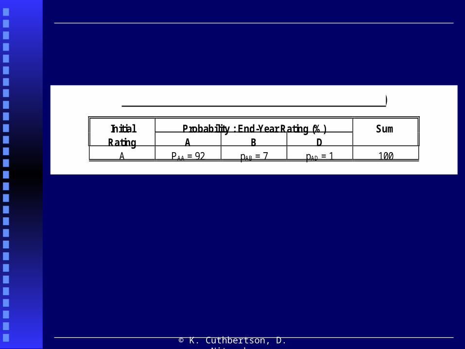
Table 25.1 : Transition Matrix (Single Bond)

Initial Probability : End-Year Rating (%) SumRating A B D

A PAA = 92 pAB = 7 pAD = 1 100


Table 25.2 : Recovery Rates After Default (% of par value)

Seniority Class Mean (%) Standard Deviation (%)Senior Secured 53 27Senior Unsecured 51 25Senior Subordinated 38 24Subordinated 33 20Junior Subordinated 17 11


Table 25.3 : One Year Forward Zero Curves

Credit Rating f12 f13 f14

A 3.7 4.3 4.9B 6.0 7.0 8.0

Notes : f12 = one-year forward rate applicable from the end of year-1 to the end of year-2 etc.


Table 25.4 : Probabilities and Bond Value (Initial A-Rated Bond)

Year End Rating Probability % $ValueA pAA = 92 VAA = 109B pAB = 7 VAB = 107D pAD = 1 VAD = 51

Notes : The mean and standard deviation for initial-A rated bond are Vm,A = 108.28, V,A = 5.78.

Mean and Standard Deviation

Vm,A = 0.92($109) + 0.07($107) + 0.01($51) = $108.28

v,A = [0.92($109)2 + 0.07($107)2 + 0.01($51)2 - $108.282]1/2 = $5.78


Table 25.5 : Probability and Value (Initial B-Rated Bond)

Year End Rating Probability $Value1. A pBA = 3 VBA = 1082. B pBB = 90 VBB = 983. D pBD = 7 VBC = 51

Notes : The mean and standard deviation for initial-B rated bond are Vm,B = 95.0, V,B = 12.19.


Table 25.6 : Possible Year End Value (2-Bonds)

Obligor-1 (initial-A rated) Obligor-2 (initial-B rated)

1. A 2. B 3. DVBA = 108 VBB = 98 VBD = 51

1. A VAA = 109 217 207 1602. B VAB = 107 215 205 1583. D VAD = 51 159 149 102

Notes : The values in the ith row and jth column of the central 3x3 matrix are simply the sum of the values in the appropriate row and column (eg. entry for D,D is 102 = 51 + 51).


Table 25.7 : Transition Matrix (ij (percent))

Initial Rating End Year Rating Row Sum1. A 2. B 3. D

1. A 92 7 1 1002. B 3 90 7 1003. D 0 0 100 100

Note: If you start in default you have zero probability of any rating change and 100% probabilityof staying in default.


Two Bonds

Requires probabilities of all 3 x 3 joint end-year credit

ratings and for each state

~ joint probability (see below)

~ value of the 2 bonds in each state (T25.6 above)


Table 25.8 : Joint Migration Probabilities : ij (percent) ( = 0)

Obligor-1 (initial-A rated) Obligor-2 (initial-B rated)1. A 2. B 3. Dp21 = pAB = 3 p22 = pBB = 90 p23 = pBD = 7

1. A p11 = pAA = 92 2.76 82.8 6.442. B p12 = pAB = 7 0.21 6.3 0.493. D p13 = pAD = 1 0.03 0.9 0.07

Notes : The sum of all the joint likelihoods in the central 3x3 matrix is unity (100). The joint migration probability i,j =p1,i p2,j (where 1 = initial A rated and 2 = initial B rated). We are assuming statistical independence so forexample the bottom right entry 33 = p13 p23 = 0.07% = 0.07x0.01x100%). The transition probabilities (eg. p12 =7%) are included as an aide memoire. The figures on the left (eg. p12 = 7%) equal the sum of the likelihood rowentries (eg. 92= 2.76+82.8+6.44) and the figures at the top (eg. p22 = 90%) equal the sum of the columnentries.

Assumes independent probabilities of migration

p(A at A, and B at B) = p(A at A) x p(B at B)


Two Bonds

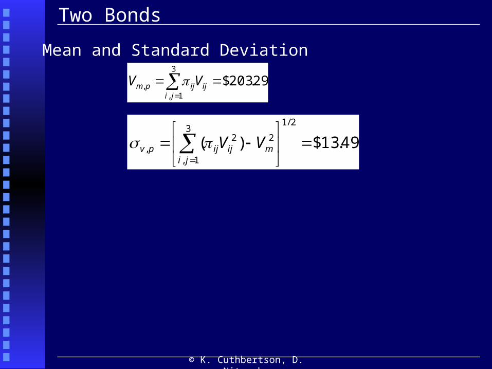
Mean and Standard Deviation

29.203$3

1,,

jiijijpm VV

49.13$)(

2/13

1,

22,

jimijijpv VV


Table 25.9 : Marginal Risk

Bond Type Standard DeviationA 5.87B 12.19

A + B 13.49Marginal Risk of Bond-B 7.62

Notes : The marginal risk of adding bond-B to bond-A is $7.62 ( = A+B - A = 13.49- 5.87), which is much smaller thanthe “stand-alone” risk of bond-B of B =12.19, because of portfolio diversification effects.

Marginal Risk of adding Bond-B


Fig 25.3: Marginal Risk and Credit Exposure

Credit Exposure ($m)

7.55 10 15

Asset 18 (BBB)

Asset 15 (B)

Asset 9

Asset 16

Asset 7 (CC)

00.0%

2.5%

5.0%

7.5%

10%

Mar

gina

l Sta

ndar

d D

evia

tion

(

p+i -

p)

/i

Source : J.P. Morgan (1997) CreditMetricsTM Technical Document Chart 1.2.


Percentile Level of C-VaR

Order VA+B in table 25.6 from lowest to highestthen add up their joint likelihoods (table 25.8) until these reach the 1% value.

[25.10] VA+B = {$102, $149, $158, $159, …, $217} i,j = {0.07, 0.9, 0.49, 0.43, …, 2.76}

Critical value closest to the 1% level gives $149Hence:

C-VaR = $54.29 (= Vmp - $149 = $203.29 - $149)


Credit VaR

The C-VaR of a portfolio of corporate bonds depends on

the credit rating migration likelihoods

the value of the obligor (bond) in default (based on the seniority class of the bond)

the value of the bond in any new credit rating (where the coupons are revalued using the one-year forward rate curve applicable to that bonds new credit rating)

either use the end-year portfolio standard deviation or more usefully a particular percentile level



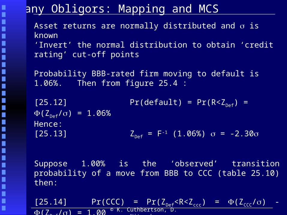
Asset returns are normally distributed and is known‘Invert’ the normal distribution to obtain ‘credit rating’ cut-off points

Probability BBB-rated firm moving to default is 1.06%. Then from figure 25.4 :

[25.12] Pr(default) = Pr(R<ZDef) = (ZDef/) = 1.06%Hence:[25.13] ZDef = F-1 (1.06%) = -2.30

Suppose 1.00% is the ‘observed’ transition probability of a move from BBB to CCC (table 25.10) then:

[25.14] Pr(CCC) = Pr(ZDef<R<Zccc) = (ZCCC/) - (ZDef/) = 1.00

Hence: (ZCCC/) = 1.0 + (ZDef/) = 2.06

and ZCCC = -1(2.06) = -2.04


Figure 25.4: Transition Probabilities: Initial BB-Rated

Probability

Transition probability:

DefCCC

B

BB BBB

A

AAAAA

-2.301.06

-2.041.00

-1.238.84 80.53

1.377.73

2.39 0.67

2.930.14

3.430.03

Standard Deviation:

We assume (for simplicity) that the mean return for the stock of an initial BB-rated firm is zero

Probability of a downgrade to B-rated

Probability of default

Z



Calculating the Joint Likelihoods i,j

Asset returns are jointly normally distributed and covariance matrix is known, as is the joint density function f

For any given Z’s we can calculate the integral below and assume this is given by ‘Y’

[25.15] Pr(ZB <R<ZBB, Z’BB <R’<Z’BBB) = dR dR’ = Y%

‘Y’ is then the joint migration probability

We can repeat the above for all 8x8 possible joint migration probabilities

),,( ''

' RRf

BBB

BB

BB

B

Z

Z

Z

Z


MCS

Find the cut-off points for different rated bonds

Now simulate the joint returns (with a known correlation) and associate these outcomes with a JOINT credit position.

Revalue the 2 bonds at these new ratings ~ this is the 1st MCS outcome, Vp

(1)

Repeat above many times and plot a histogram of Vp

Read off the 1% left tail cut-off point

Assumes asset return correlations reflect changing economic conditions, that influence credit migration


Table 25.10 : Threshold Asset Returns and Transition Probabilities (Initial BB Rated Obligor)

Final Rating Transition Prob Threshold Asset Return(cut off)

AAAAAA

BBBBBB

CCCDefault

0.030.140.677.7380.538.841.001.06

-ZAA

ZA

ZBBB

ZBB

ZB

ZCCC

ZDef

-3.432.932.391.37-1.23-2.04-2.30

Source: J.P. Morgan (1997) Table 8.4 (amended)


Table 25.11 : Individual Firm’s Transition Probabilitie

End-year Individual Transition Probabilities % Rating Firm 1(BBB) Firm 2(A) Firm 3(CCC)

AAAAAA

BBBBBB

CCCDefault

0.020.335.9586.93

---

0.18

0.092.27

91.055.52

---

0.06

0.220.000.221.30

---

19.79Sum 100 100 100

Source: J.P. Morgan (1997) Table 9.1


Table 25.12 : Asset Return Thresholds

Threshold Firm-1 (BBB) Firm-2 (A) Firm-3 (CCC)ZAA

ZA

ZBBB

ZBB

ZB

ZCCC

ZDef

3.542.781.53-1.49-2.18-2.75-2.91

3.121.98-1.51

--

-3.19-3.24

2.862.862.63

--

1.02-0.85

Notes: The Z’s are standard normal variates. For example, if the standardised asset return for firm-1 is –2.0 then thiscorresponds to a credit rating of BB. Hence if ZB R ZBB then the new credit rating is BB. If from run-1 of the MCS weobtain (standardised) returns of -2.0, -3.2 and +2.9 then the ‘new’ credit ratings of firm’s 1, 2 and 3 respectively would beBB, CCC and AAA respectively.

Source: J.P. Morgan (1997) Table 10.2


Other Models


KMV Credit Monitor

Default model~ uses Merton’s , equity as a call option

Et = f(Vt, FB, v, r, T-t)

KMV derive a theoretical relationship between the unobservable volatility of the firm v and the observable stock return volatility E:

E = g (v)

Knowing FB, r, T-t and E we can solve the above two equations to obtain v.

Distance from default = std devn’s

If V is normally distributed, the ‘theoretical’ probability of default (i.e. of V < FB) is 2.5% (since 2 is the 95% confidence limit) and this is the required default frequency for this firm.

210

80100)1(

v

Bv FV


Uses Poisson to give default probabilities and mean default rate can vary with the economic cycle.

Assume bank has 100 loans outstanding and estimated 3% p.a. implying = 3 defaults per year.

Probability of n-defaults

p(0) = = 0.049, p(1) = 0.049, p(2) = 0.149, p(3) = 0.224…p(8) = 0.008 ~ humped shaped probability distribution (see figure 25.5).

Cumulative probabilities:p(0) = 0.049, p(0-1) = 0.199, p(0-2) = 0.423, … p(0-8) = 0.996“p(0-8)” indicates the probability of between zero and eight defaults in Take 8 defaults as an approximation to the 99th percentile Average loss given default LGD = $10,000 then:

!),(

n

edefaultsnp

n

CSFP Credit Risk Plus


Average loss given default LGD = $10,000 then:

Expected loss = (3 defaults) x $10,000 = $30,000

Unexpected loss (99th percentile) = p(8) x 100 x 10,000 = $80,000

Capital Requirement = Unexpected loss-Expected Loss = 80,000 - 30,000 = $50,000

PORTFOLIO OF LOANSBank also has another 100 loans in a ‘bucket’ with an average LGD = $20,000 and with = 10% p.a.

Repeat the above exercise for this $20,000 ‘bucket’ of loans and derive its (Poisson) probability distribution.

Then ‘add’ the probability distributions of the two buckets (i.e. $10,000 and $20,000) to get the probability distribution for the

portfolio of 200 loans (we ignore correlations across defaults here)

CSFP Credit Risk Plus


Figure 25.5: Probability Distribution of Losses

Loss in $’s

Probability

Unexpected Loss

Expected Loss

Economic Capital

$30,000 $80,000

0.224

0.049

0.008

99th percentile


Explicitly model the link between the transition probability (e.g. p(C to D)) and an index of macroeconomic activity, y.

pit = f(yt) where i = “C to D” etc.

y is assumed to depend on a set of macroeconomic variables Xit (e.g. GDP, unemployment etc.)

Yt = g (Xit, vt) i = 1, 2, … nXit depend on their own past values plus other random errors it. It follows that:

pit = k (Xi,t-1, vt, it)

Each transition probability depends on past values of the macro-variables Xit and the error terms vt, it. Clearly the pit are correlated.

McKinsey’s Credit Portfolio View, CPV


Monte Carlo simulation to adjust the empirical (or average) transition probabilities estimated from a sample of firms (e.g. as in CreditMetrics).

Consider one Monte Carlo ‘draw’ of the error terms vt, it (which embody the correlations found in the estimated equations for yt and Xit above).

This may give rise to a simulated probability pis = 0.25 of whereas

the historic (unconditional) transition probability might be p ih = 0.20 .

This implies a ratio of

ri = pis / pi

h = 1.25

Repeat the above for all initial credit rating states (i.e. i = AAA, AA, … etc.) and obtain a set of r’s.



Then take the (CreditMetrics type) historic 8 x 8 transition matrix Tt and multiply these historic probabilities by the appropriate ri so that we obtain a new ‘simulated ‘transition probability matrix, T.

Then revalue our portfolio of bonds using new simulated probabilities which reflect one possible state of the economy.

This would complete the first Monte Carlo ‘draw’ and give us one new value for the bond portfolio.

Repeating this a large number of times (e.g. 10,000), provides the whole distribution of gains and losses on the portfolio, from which we can ‘read off’ the portfolio value at the 1st percentile.

Mark-to-market model with direct link to macro variables



TABLE 25.13 : A COMPARISON OF CREDIT MODELS

Characteristics J.P.MorganCreditMetrics

KMVCredit Monitor

CSFPCredit Risk Plus

McKinseyCredit Portfolio

ViewMark-to-Market(MTM) or DefaultMode (DM)

MTM MTM or DM DM MTM or DM

Source of Risk Multivariate normalstock returns

Multivariate normalstock returns

Stochastic defaultrate (Poisson)

MacroeconomicVariables

Correlations Stock pricesTransition

probabilities

Option pricesStock pricevolatility

Correlation betweenmean default rates

Correlation betweenmacro factors

Solution Method Analytic or MCS Analytic Analytic MCS


End of Slides

© k. cuthbertson, d. nitzsche financial engineering: derivatives and risk management (j. wiley,...

Documents

nitzsche slide

bondb slide

mcs slide

nitzsche credit var

standard deviation slide

b d slide

nitzsche creditmetrics

nitzsche fig