•

•

. -. -~... ~. --. -.<-_.- .~~

. __,' : I. _.._.- "', ..---- -'T---'" -_ ... "j ......

........._- _._- _._,_ ~-- -~ ~.,,~,.,.. ,. I

,PROPORTIONAL ODDS AND PARTIAL PROPORTIONALODDS MODELS FOR o~tfINAL'-RESl?ON~E" VARIABLES

. ~_ .••. ' t • .~._-_---r,'--4""~' ~ .hA.· --- --- """, ~-_. ~.,.

b .,-,-~,",.I-,,-_-,-_..¥.... !:.....__ ..._.....

'0 iBerced~~s.c..:.Le.ola .. Pe.t.erson""',:-::"

DepartITienl:-"ot-l::ftosEatisticsUniversity of North-CarO~ina at Chapel Hill

Institute of Statistics Mimeo Series No. 1809T

October 1986

•

PROPORTIONAL ODDS AND PARTIAL PROPORTIONAL ODDS MODELS

FOR ORDINAL RESPONSE VARIABLES

by

Bercedis Leola Peterson

A Dissertation submitted to the facultyof the University of North Carolina atChapel Hill in partial fulfillment of

the requirements for the degree ofDoctor of Philosophy in the Department

of Biostatistics

Chapel Hill

1986

Approved by:

•

ABSTRACT

BERCEDIS LEOLA PETERSON. Proportional Odds and PartialProportional Odds Models for Ordinal Response Variables.(Under the direction of Frank E. Harrell, Jr.)

The logistic linear regression model for a binary

response variable (see Walker and Duncan, 1967, section 3)

has been extended to allow for an ordinal response variable

that takes on k+l possible values (Walker and Duncan, 1967,

section 6; also described later by McCullagh, 1980). The

resulting analysis fits a set of k cumulative logits to.

linear functions of the explanatory variables so that k

models are formed. The regression coefficients are

identical across the k models, except for the intercept

terms, ~j' j=l, ••• ,k, which are ordered to reflect the order

of the cumulative probabilities.· The assumption of

identical regression coefficients across models is referred

to variously as proportional odds (McCullagh, 1980), uniform

association (Agresti, 1984), and homogeneity of category

boundaries across subpopulations (Williams and Grizzle,

1972).

Although Koch, Amara, and Singer (1984) suggest a test

for the validity of this assumption, a test based on maximum

likelihood procedures has not appeared. This dissertation

develops such a test as well as a maximum likelihood

procedure for fitting a model that does not require

iii

proportional odds. In addition, simulations are presented

to compare the power and Type I error rates of the procedure

p~oposed by Koch, Amara, and Singer with the newly developed

procedure based on maximum likelihood. Finally, graphical

methods for assessing the proportional odds assumption of

the ordinal logistic model are discussed, and the new

procedures are demonstrated using cardiovascular disease

data.

•

iv

ACKNOWLEDGME~~S

My sincerest thanks go to the three men who made it

possible for me to write this dissertation: Frank Ha~~ell,

John Barefoot, and David Shore. Dr. Harrell suggested the

topic and gave me constant guidance and encouragement~

without him this paper would not have been possible. Dr.

Barefoot, my boss, allowed me to use work time to do my own

research. And, David, my husband, was totally supportive

and gave me the emotional strength to do what had to be

done.

Finally, to the four members of my advisory committee:

you were very kind to me, and I am grateful to you for your

time and encouragement. Thank you, Drs. Gary Koch, Dave

Kleinbaum, Larry Kupper, and Vic Schoenbach .

ACKNOWLEDGMENTS ..

LIST OF TABLES ..

LIST OF FIGURES

CHAPTER

TABLE OF CONTENTS

. . . . . . . . . . . . . .

v

Page

iv

· . vii

· . vii i

1. INTRODUCTION AND REVIEW OF THE LITERATURE · 1

1.1 Introduction · · · · · · · · · · · · · 11.2 Koch, Amara, and Singer's Model · · · 151.3 Anderson's "Stereotype" Model · · · · · · 191.4 Nonparametric Competetors to the Ordinal

e Logistic Model · · · · · · 24

I I • MODELS AND STATISTICS · · · · · · · · · · · · · 27

2.1 The Partial Proportional Odds Model · · · 272.2 The Maximum Likelihood Solution · · · 292.3 Score Test of the Proportional Odds

Assumption • · · · · · · · · · · · · · 342.4 The "Constrained" Partial Proportional

Odds Model . · · · · · · · · · · · · · 422;5 A Computer Program to Obtain Statistics

from the Partial Proportional Odds Model · 45

2.5.1 Wald Statistics · · · · • · · • · · 452.5.2 Score Tests of Proportional Odds. · 462.5.3 Tests of the Goodness of Fit of

the Constrained PartialProportional Odds Model · · · · · · 47

2.5.4 Limitations of the ComputerProgram · · · · · · · · · · 49

.. I I I • INVALIDITY IN THE SCORE AND WALD TESTS 50

3.1 Introduction · · · · • · 503.2 Detection of Ill-Conditioning in the

Information Matrix · · · · · • • · 563.3 Detection of Invalidity in KAS's

Wald Statistic · · · · · · · · · · · · 613.4 Simulation Results · · · · · · • · 64

vi

IV. THE SIMULATIONS · · · · · · · · · · · ·4.1 Introduction · · · · · · · · · · · ·4.2 Design 1 · · · · · · · · · · · ·4 ~ Design 2 · · · · · · · · · · · ·.-4.4 Design 3 · · · · · · · · · · · ·4.5 Design 4 · · · · · · · · . .4.6 Design 5 · · · · · · · · · ·4.7 Design 6 · · · · · · · · · · · · · ·4.8 Design 7 · · · · · · · ·4.9 Design 8 · · · · · ·4.10 Design a.- · · · · · · · · · · · ·4.11 Design 10 · · · · · · · · · · · · · ·4.12 Summary of Simulation Results · · · ·

73

737876808183868891949698

V. A DATA ANALYSIS STRATEGY · . . . . 104

5.1- ?0._

5.35.45.55.6

Introduction . . . . . . . . . • . 104Graphical Methods for AssessingProportional Odds . . . • . •. . .. 104A Data Analysis Strategy . . ..... 113Example 1 . . . • •. 117Example 2 • • .. ..•.•. .. 123Example 3 . . . . • . . . . . • . 125

VI. SUMMARY AND SUGGESTIONS FOR FUTURE RESEARCH •• 133 ~

6.16.26.36.4

APPENDICES

Introduction • •. •.•... 133Problems with the Test Statistics .•.• 134Questions of Power •••.....••.• 138Programming Suggestions . . . •• .. 140

1. COMPUTATIONAL METHOD"FOR GENERATINGSIMULATED DATA FOR THE KOCH, AMARA, ANDSINGER WALD TEST • • • • • • • • • • • • • • • 142

BI BLl OGRAPHY • • . • • • • • • • • • • • .

2.

3.

COMPUTATIONAL METHOD FOR GENERATINGSIMULATED DATA FOR THE SCORE TEST OFPROPORTIONAL ODDS • • • • • • . •

PROGRAM FOR GRAPHICALLY ASSESSINGTHE PROPORTIONAL ODDS ASSUMPTION

146

148

150

vi i

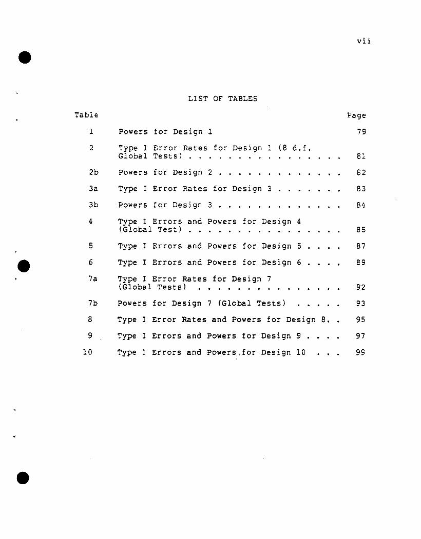
LIST OF TABLES

Table Page

1 Powers for Design 1 79

2 Type I E:-ror Rates for Design 1 (8 d. f.Global Tests) . . · · · · · · · · · · · · 81

2b Powers for Design 2 · · · · · · · · · 62

3a Type I Error Rates for Design 3 · · · · · · · 83

3b Powers for Design 3 · · · · · · · · · 84

4 Type I Errors and Powers for Design 4(Global Test) · · · · · · · · · · · · 85

5 Type I Errors and Powers for Design 5 · · · · 87

e 6 Type I Errors and Powers for Design 6 · · · · 89

7a Type I Error Rates for Design 7(Global Tests) . · · · · · · · · 92

7b Powers for Design 7 (Global Tests) · · · 93

8 Type I Error Rates and Powers for Design 8. · 95

9 Type I Errors and Powers for Design 9 · · 97

10 Type I Errors and Powers.. for Design 10 · · · 99

F·igure

1

2

3

4

5

6

7

8

LIST OF FIGURES

Odds Ratios for Relationship BetweenCardiovascular Disease and Smoking Status

Odds Ratios for the Relationship BetweenCardiovascular Disease and Duration 0:Symptoms, Dichotomized at the Median ..

Odds Ratios for the Relationship BetweenCardiovascular Disease and Duration ofSymptoms (Odds Ratios Estimated by MaximumLikelihood •...•..•.•......

Proportions of CAD> j (j=l-S) vs. CADDUR(CADDUR Grouped into 10 Quantile Groups)

Odds Ratios for the Relationship BetweenCardiovascular Disease andHypercholesterolemia • • • • • • • • • •

Results of a Maximum Likelihood Analysisof Example 1 • . • • • . • • • • . . . •

Results of a Maximum Likelihood Analysisof Example 1 • . • • • . • • . . . • . .

Results of a Maximum Likelihood Analysisof Example 2 • • • • • • • • • • . . • •

viii

PagE

106

lOS

110

112

118

121

122

124

..

9

10

11

12

13

Results of a Maximum Likelihood Analysisof Example 3 (Steps 1 and 3) ••••••

Odds Ratios for the Relationship BetweenCardiovascular Disease and Sex • . • • •

Odds Ratios for the Relationship BetweenCardiovascular Disease and Age •..••

Results of a Maximum Likelihood Analysisof Example 3 (Steps 4 and 5) ••••.•

Results of a Maximum Likelihood Analysisof Example 3 (Step 6) .•••..•••

· . .

· . .

· . .· . .

126

127

128

130

132

CHAPTeR I

INTRODUCTION AND REVIEW OF THE LITERATURE

1.1. Introduction to Ordinal Response Models

Lite~ature on the analysis of o~dina1 data can be

classified as dealing either with measurement of association

or model building, although naturally these two

classifications often overlap. Within the latter catego~y,

two distinct types of models exist. In the loglinear model

a cross-classification table containing at least one ordinal

variable is analyzed in terms of associations and

interactions among all the variables. Agresti (1984) and

Bishop et ale (1975) thoroughly examine this model. In the

other type of model, one variable, an ordinal variable, is

considered a response variable to be explained by the

remaining set of variables. Structural relationships among

the set of explanatory variables is ignored. This paper is

concerned only with the latter type of model.

Although many ordinal response models have been

suggested, some have attracted greater interest than others.

Mean response, logistic, and probit models are among the

more widely used. These three models can be thought of as

generalizations of simpler models in which the response

variables are binary. For the discussion, let Y denote a

response variable that can assume only two values, say 0 and

2

1, so that the expected value of Y, denoted by P, is the

probability that Y=l. The standard linear model is often

used to model this expected value as a function of a set of

explanatory variables:

( 1 )

Here, ~ is the expected value of Y for the ith observation,

X. is a design vector whose elements are observation i's-.values on p explanatory variables, and ~ and $ are unknown

~

parameters to be estimated. This model is usually fitted

using weighted least squares.

If i indexes not individual observations but

subpopulations having n~ observations, i=l, ... ,s, and if ~;

is a design vector with coding for group membership, then

the data can be represented by a cross-classification table

with sx2 cells. In this situation, ~ is the probability

that v -. - 1 within subpopulation i. If i indexes

individuals, however, then the model can take a more general

form, where the p elements of ~; can be either observed

values on continuous variables or a coding indicating group

membership.

For the case where i indexes subpopulations, several

authors have extended model (1) above to permit an ordinal

response variable. For example, if the score ~ is assigned

to the jth response category of an ordinal variable, then

the mean of Y within each subpopulation can be used as the

response function. If n;j is the number of observations in

3

subpopulation i with score ~ , then the subpopulation mean

can be calculated asY. = ~y. n.. In;. ,. and the expected value.. j J OJ

of the mean c·an be modeled as

E(~·) = 0( + x:~ .~ ..... - ( 2 )

Bhapkar (1968), Grizzle et all (1969), and Williams and

Grizzle (1972) suggest this model and present weighted least

squares solutions. Models similar to the one above have

also been used in which the response scores are suggested by

the data. These scores take the form of rank function

measures such as ridits. Agresti (1984) discusses some of

the literature in this area.

When Y is binary, model (1) above is not the most

appropriate model. As Neter and Wasserman (1974), among

others, point out, a good form for a probability model is

the logistic model:

PI =1

1 + exp (- D( -~~ ~

Simple algebraic manipulations allow this model to be

linearized as

= 0( + X~ $ •.... -P'..In

1 - p.

For the case where i indexes subpopulations, Cox(1970)

presents several ways to estimate and test the regression

parameters in this model. One of his methods, a weighted

least squares approach, is also described in detail by

Grizzle et al. (1969) and Theil (1970). When i indexes

4

individuals and the explanatory variables are a mixture of

continuous and categorical variables, Walker and Duncan

(1967) and Cox (1970) show how maximum likelihood methods

can be use:c ~c est ima tEo -< ana f.The logistic model has been extended to include cases

where the dependent variable has several categories. If the

categories of the dependent variable can be considered

ordered, then several ways of forming a set of logits are

available. Let ~ denote the probability that a randomly

selected observation falls in the j~h response category,

j=O,l, ... ,k. Then accumulated or cumulative logits are

defined by

In(~~ /££PL ), j=1,2, ... ,k,hj I~j

continuation ratio logits by

1 n (Pj / 1~P1 ), j =1 , 2 , • • • , k ,J

and adjacent categories logits by

1n (P. /P. \), J' =1 , 2 , ••• , kJ J-

(Agresti, 1984). These three sets of logits take category

order into account. Another set of logits that is

appropriate even for unordered categories is the polytomous

10git defined by

InPoi / (po + Pj )

Po / (PD + Pj= In(Pj/Po )' j=1,2, ••• ,k.

5

This logit is also called a conditional logit, since it is

the log odds of being in category j instead of category 0,

conditional upon being in one of these two categories. This

set of logits can handle any ca=egoric61 dependent variable,

but cannot readily incorporate information on ordering if

such information is available. Anderson (:984), however,

does use it in the development of his "stereotype" model for

ordered categorical variables. This model will be discussed

later.

The cumulative logits discussed above are the focus of

this paper. In the literature, the model for these logits

has frequently been interpreted under the assumption of an

underlying, unobservable, continuous random variable, Z,

whereby an observation is classified into category j if the

observation falls between Lj and Lj+1 (e.g., Plackett, 1981).

These division points are assumed unknown and can be

estimated by the model. Although the assumption of an

underlying continuum is not essential for interpretation of

the model, such an assumption does make the interpretation

"direct and incisive" (McCullagh, 1980). Anderson (1984),

likewise, claims that the model is "most appropriate when

the categories are related monotonically to an unobservable,

continuous variable."

The problem of relating an observed ordinal response to

an underlying quantitative response is considered in detail

by Hewlett and Plackett (1956) in the context of the

biological assay. They claim that the quantal dose-response

6

relationship can be derived from the corresponding

quantitative dose-response relationship, in that every

quantal response is the result of an underlying graded

response reaching a cer~ain level of intensity. In the

literature, data arising by such a partition of an

underlying continuous distribution are usually modeled by

using either the logistic or the normal distribution to

define the cumulative probabilities. For example, the

normal distribution has been used in the area of biological

assay by Ashford (1959) and Gurland et ale (1960), and in

entomology by Aitchison and Silvey (1957). In biological

assay the problem is usually to predict a response to a drug

given the dose administered. When the response is assumed

to have an underlying normal distribution, then the

probability of an observation with the ith dosage falling in

or above response level j of an ordinal variable, Y, is

given by the probit model(!110

Ci~ = Pr (Y ~ j I1) = ~~ j ~- '3"/,..,~

7'j -}I.D""

,j=l, ••• ,k, ( 4 )

where the response categories are coded O,l, •.• ,k, and the

choice of category is controlled by a response process Z

distributed N(fI... , c?'). Here, t'j is the threshold value

corresponding to the lower boundary of category j, and thus

these'S define successive intervals on the underlying

continuum. Another way to write this model is to let

cXj = OCJ/Cf and ~ = -,Pi-It/' so that ('Cj - p..J/tJ' = o(j + a~. Note

7

that the inverse normal functions corresponding to the

probabilities in model (4) define the normits

..,:-1y.J (C·) =IJ

"",.... o.J p .... ( 5)

•When the response is assumed to have an underlying

logistic distribution, the model is

Cij = Pr (y ~ j /~;) =1 + exp [- O<j - ~~E ]

j=l, ... ,k,

where ~,> ~~ >"'>~k' Appropriate algebraic manipulation

of the above equation gives the cumulative logits

•In

CooOJ = a<J' + ~.' I') )'-1 k- p, -, • • ., •..... ( 7 )

Use of the logistic distribution to define the cumulative

probabilities in terms of just one continuous explanatory

variable was initiated by authors such as Gurland et ale

(1960). Several authors later extended the model to include

a mixture of continuous and categorical explanatory

variables, although Walker and Duncan (1967) were the first

to publish a method for fitting this more general model.

In a special case of this model frequently seen in the

literature, group membership in one of s subpopulations is

used to predict Y. If i is used to index the populations, so

that Cu = Prey ~ j/i), then the model can be written

InC·,

IJ

1 - Cj~

= a{j + ~~ , i =1, ••. , s,j =1, ••• , k •

(8 )

8

I dent i f iabi 1i ty of ·the parameters can be assured by a.s

cot'ldi t ion such as ~ e4 = 0 or ~s = 0, where the ~A. are the'-1

population effects (Plackett, 1981). This model is, of

course, J'ust mode: (7) above ex~ept that the elements of I·-4

are either 0 or 1 to indicate group membership. If an

underlying continuum is assumed, then in both these models

the oXj are the category division points on a logit scale.

Notice in these models that given any two distinct values of

i, the log odds ratio remains constant across all choices of

j, j=l, ... ,k. That is, in terms of model (7), the log odds

ratio,

InCoo / (l-C·· )IJ ,,,)

C· .... / (I-C·,. )• ,) IJ

= (0" +X.' ~ ) - (0<:. +X' ~ ) =J ........ J"'~" "'"

does not depend on j. This aspect of the model is called

proportional odds.

Note that if ~ in model (7) above were replaced with,..

~j (or if $~ in model (8) were replaced with Pij), then it

would be possible to get

InCoO

'J < 1nCoO'"OJ

, j < j',

so that Coo ... > C", But this is obviously not permissibleIJ IJ

under the assumption of a single underlying distribution.

Walker and Duncan (1967) use an example where subjects are

classified as having suffered myocardial infarction (Y=2),

angina pectoris (Y=l), or are considered free of disease

..

•

"

9

(Y=O). To paraphrase Walker and Duncan, the only way the

probability of having at least angina pectoris could be less

than the probability of having just an infar~tion would be

if ~ we~e sufficient to entail an infarctior. but not

sufficient to entail the less severe angina pectoris. If

myocardial infarction and angina pectoris are indeed grades

of severity of the same disease, then this could not occur.

Thus, the model assumes that Y represents grades of

intensity of a single underlying dimension. Walker and

Duncan explain that this assumption is seen in the fact that

c.o j > Coj"" for j < j', if and only if the "slope" coefficient

is identical for each logit.

If an underlying continuum, Z, for the ordinal variable

Y is assumed, then the proportional odds probit and logit

models above imply that the category boundaries and the

variance of the underlying latent variable do not depend on

~. Since this may not be immediately obvious from looking

at the model, an explanation follows. The assumption of

identical category boundaries will be discussed first, and

then the assumption of constant variance.

If an underlying continuous distribution is assumed,

the use of ~..j instead of ~.;, in model (8) above (or ~j

instead of ~ in model (7» permits an interaction between

the categories of the response variable and the

subpopulations (Williams and Grizzle, 1972). These authors

point out that this interaction indicates that the

categories of response have different category boundaries

10

for the different subpopu1ations. If this point is not

clear, consider this simple example. Suppose that an

underlying continuous random variable, Z - U(1,10), has been

t~ansformeo into a three-level ordinaJ. ~andom variable, Y.

Further suppose that for one subpopulation, the category

boundaries used to make this transformation are at Z = 4 and

Z = 5, whereas for another subpopulation the boundaries are

at Z = 3 and Z = 6. Finally suppose that Z is identically

distributed within the two subpopulations. If in each

subpopulation nine observations are sampled with values on Z

of 1.5,2.5, ... ,9.5, then even though no difference between

the groups on the continuous variable Z exists, the

resulting crosstabulation of the data would reveal

otherwise, Le.:

xo 1

+------+-------+0 I 3 I 2 I+------+-------+

Y 1 I 1 I 3 I+------+-------+2 -, 5 I 4 I+------+-------+

Further, the log odds ratios corresponding to the two

cumulative probabilities would not be equal to each other or

to 0 even though the distribution of Z is the same in the

•

two subpopulations. Forcing the log odds ratios to be

equal, Le., requiring ~;I = ~;.~ =... = tk is sensible only

if the category boundaries are identical for each

subpopulation.

Now consider the assumption of constant variance on the

•

..

•

11

underlying continuum across the subpopulations. Bock (1975)

and McCullagh (1980) have presented non-linear probit and

logit models, respectively, that do not require this

assumption. McCullagh's model is

(.. O<j + X~eIn 'J -.. «:.. ~.' ~.i. ( 9 )= = +

"t"..: .J1 - C·. ....

AJ

where X~~ and ~ are called, respectively, the "location",..-and "scale" for the i-th population. In McCullagh's words,

~his model permits "shifted distributions" on the underlying

continuum. Bock's model is very similar to McCullagh's,

being just the probit model given earlier with ~ allowed toI

vary with subpopulation. Bock refers to the assumption of

constant variance as the assumption of "homogeneity of the

response-process dispersions." A test for constant variance

involves test ing whether the 't"... or 0:. ' i = l, ..• , k, are

equal.

The interpretation of the proportional odds assumption

in terms of an underlying continuum for Y is only one way to

view the model. Proportional odds also straightforwardly

asserts that the odds ratio for the association of a

dichotomized ordinal response variable with a predictor

variable is the same regardless of how the response variable

is dichotomized. For example, suppose Y, an ordinal

variable describing severity of cardiovascular disease, is

being predicted by smoking status. Then a constant odds

ratio simply implies that the association between smoking

12

status and disease is the same whether disease is

dichotomized as 'no disease/some disease' or 'at most mild

disease/more severe disease' or 'at most moderate

disease/most severe disease'.

Estimation of the regression parameters in models (7)

and (8) above is discussed by several authors. Maximum

likelihood analysis of model (8) is discussed by Snell

(1964), Bock (1975), Simon (1974), ana McCullagh (1977,

1978), all of whom handle the requirement of constant

population effects across logits by incorporating this

restraint into their maximum likelihood equations. These

authors differ, however, in their reference to the

underlying continuous distribution. Both Simon and

McCullagh ignore this distribution, being most interested in

differences among the subpopu1ations on Y. Bock

acknowledges the underlying distribution and stresses that

the model can be used to estimate the "thresholds" or

category boundaries of Z. To do this, of course, he calls

upon the assumption of homogeneity of the category

boundaries across the subpopulations. Snell's main goal is

to develop a method of determining category boundaries or

scores for the ordinal response variable, so that these

scores can then be used in analyses dependent upon the

assumption of normality. Both Bock and Snell work with the

logistic distribution only because it is very similar to the

normal distribution, but simpler to use.

William and Grizzle (1972) use the weighted least

•

...

13

squares methods developed by Grizzle et ale (1969) to

analyze a table with two categorical explanatory variables

and one ordinal response variable. The model they use is a

modification of model (8): the ~ are repla=ed by ~ so

that the regression coefficients are dependent upon j.

These authors were most interested in a test for the

homogeneity of category boundaries across several

populations and thus develop a test of identical population

effects across all k logits, i.e., in the notation used

above, a test of g;. = ~.:.. = ••• = $;." for all i. As an aside,

it may be pointed out that these authors, having accepted

the hypothesis of homogeneity, test the main effects of

their explanatory variables by averaging the ~~ across the k

logits.

For the simple case of two subpopulations, Clayton

(1974) presents a solution to model (8) using the method of

weighted least squares with empirically estimated weights

applied to the k log odds ratios. For a simple analysis

having only one explanatory variable, Gurland et ale (1960)

use the minimum logit chi-square method to obtain a solution

to model (7).

Model (7) in its most general form was first fitted by

Walker and Duncan who apply a maximum likelihood procedure

to provide estimates of the regression parameters and their

variance-covariance matrix. This model is also discussed in

a paper by McCullagh (1980) in which he links several

different models for the analysis of ordinal response data.

14

All of his models permit the assumption that the response

categories form successive intervals on a continuous scale,

although :his assumption is not necessaiy. McCullagh calls

model (7) the proportior.al odds model since the ratio of

odds for any two values of ~ does not depend on which

cumulative probability is used. Because of this attribute,

~ car. be used in model (7) instead of ~. Thus, we see that

Williams and Grizzle's test is a test for proportional odds.

The logistic model discussed by Walker and Duncan and by

McCullagh is elaborated upon by Anderson and Philips (1981).

In particular, they give maximum likelihood estimation

procedures for three different sampling schemes: (1)

sampling from Y conditional on ~ as in the prospective

study, (2) mixture sampling or sampling from the joint

distribution of Y and! as in the cross-sectional study, and

(3) sampling from X conditional on Y as in the retrospective~

study.

In conclusion, note the similarity between tests of

proportional odds and the use of time-dependent covariates

in Cox's proportional hazards model. Tests of significance

of the interaction between a covariate and some function of

time are comparable to tests of partial proportional odds in

the ordinal logistic model. In the survival model, we test

to determine if the effect of the covariate varies with

time, while in the ordinal logistic model, we test to

determine if the effect of the covariate depends on the

cumulative logit.

15

1.2. Roch, Amara, and Singer's Model

Roch, Amara, and Singer (1985)' discuss a generalization

of logistic model (7) above in which. both f and ~~ are

allowed ~o vary with j. Thus, no: only may the proportional

odds assumption not hold, but the cumulative logits may be

functions of different sets of explanatory variables. In

the notation used in this paper, the model 1S

lnc··'J , j =1, ••• , k , (10)

..

•

where x.. and $. are vectors of length t... When the X.. do• 'J .. ,) .. -"j

not depend on j, the authors use the model as an

unrestricted model for developing a test of the proportional

odds assumption. This model calls to mind the model of

Williams and Grizzle (1972) discussed previously, with the

exception that Williams and Grizzle deal only with

categorical explanatory variables. Under the assumption

that all cell counts are large enough to have a multivariate

normal distribution, Williams and Grizzle use weighted least

squares to fit their model and test the assumption of

proportional odds. Their technique, however, is not

appropriate when one or more explanatory variables are

continuous or when some cell counts are small. The Roch,

Amara, and Singer (RAS) paper thus suggests using a two­

stage method of estimation called functional asymptotic

regression methodology (FARM), described by Imrey et ale

(1981).

"confused with the ~ in model (7».....

16

In the first stage of this procedure separate maximum

likelihood analyses are used to estimate each of the k

cumulative logits, In[Pr(Y ~ j)/Pr(Y < j»)~ thus each

analysis is a logistic regression using a binary response

variable. Simultaneous goodness of fit of these preliminary

models is assessed through a residual score statistic having

an approximate chi-square distribution. Since this

statistic is of little relevance to our paper, it will not

be discussed. Let it suffice to say that this statistic

tests whether the set of models would be significantly

improved if additional columns, ~, were added to e. These

extra columns typically correspond to higher order

interaction terms.

"From these preliminary models are obtained ~~ of length.. "

sand varianceY(IJ)' j=l, ... ,k. The ~j are concatenated"into one longer vector of length t = ~ tj to get ~ (not to be

J ...

If proportional odds is

to be tested, the same set of explanatory variables is used

for each cumulative logit so that to =t~= ..• tK = p+l and

t = k(p+l). Note that the maximum likelihood estimate of

"the variance of 2~ can be written as:

= (X'D.. X)""" ... JJ ..

where !' = (!tI ' • • • , ~"') and Pij i sadi agonalmat r i x 0 f s i ze

n x n with functions of the predicted probabilities from the

model on the diagonal. That is,

•

Cr-

•

17

D.. = diag[C ,J" (1-C ,i ), ••• ,C",.(1-C",')].-.lJ II J ~

,.. "-

The covariance between B. and RJ·, can be written as:NJ

where

(The definition of ~jj/ given here is slightly different from

in the KAS paper, since they predict Pr(Y ~ j) whereas we

"predict Pr{Y ~ j).) The variance of ~, y!, can now be

written by defining a matrix that has the ~ terms as block

diagonal components and the Yjj/ terms as blocks on the off­

diagonal.

The proportional odds structure of the model can be

tested by using the Wald statistic given by:,. I "

Q~ = ~ t ~ t (~y! £t f ~e (11 )

where £ is a contrast matrix of rank c, and Qc has an~ -

approximate ~~ distribution under the null hypothesis.

can be chosen to test proportional odds for any subset of

the p explanatory variables.

If the proportional odds assumption is found to hold

for one or more explanatory variables, then in the second

stage of the FARM analysis new regression coefficients that

take proportionality into account are estimated using

weighted least squares to fit models of the form:

..E(~ ) = z'l,.. ... -

Here, z is a constant matrix of full rank u and size.-

18

k(p+l) x u, and 1 is a uxl vector of unknown second-stage

parameters to be estimated. The weighted least squares

estimate of '( is givE:n by:

t = (Z' v~ Z f' z.v,J..., ""'" ""'f.... - 'V ~ -

and its variance is estimated by:

A

v( ~ ) = (Z'v ... Z)-I._ N ,.,.. -~ ."

,..

The Wald chi-square goodness of fit test for reduction of

the space spanned by ~ to the space spanned by r has

k(p+l)-u degrees of freedom and is given by:

A nonsignificant value from this test implies that the....

expected value of? is adequately modeled by ~t.,.

As an example, if a three-level ordinal response

variable is to be predicted by one explanatory variable x,

the initial model

= X.' ~. = e( , +~. x , j =1 , 2 ,-A ... J .. JIn

is used to get

c·,AJ

1 - C.,;... " ,. "~ = (&., VI 0<. ... ~~)'. The Wald statistic is

then used to test PI =~J by using £ = (0 1 0 -1). If this,..

hypothesis is accepted, the final two-stage model E{f) = ~!

is fitted with •

z =

) , . In this simple example, the Wald

19

goodness of fit statistic in (12) would be identically equal

to s~atistic (11).

The final model developed using statistic (12) above

permits partial proportionality in that some explanatory

variables may meet the proportionality assumption, while

others may not. However, statistic (11) does not allow the

assumption of proportional odds to be tested for one set of

variables while constraining another set to have

proportional odds.

The authors note that a maximum likelihood estimation

procedure might be considered for fitting model (10),

although they give two reasons why such a procedure might be

"computationally less attractive" than the FARM procedure.

One, "it may require specialized iterative algorithms

formulated on an individual model basis," and two, "the

design of such algorithms may be further complicated by the

need to avoid zero or negative probabilities at each

iteration." If these problems can be surmounted, however, a

maximum likelihood procedure may have more desirable

properties than a procedure that uses Wald tests (Hauck and

Donner, 1977) or weighted least squares. Furthermore,

unlike the first stage of the FARM procedure, a maximum

likelihood procedure takes the covariance structure among

the k cumulative probabilities into account.

1.3. Anderson's "Stereotyoe" Model

As mentioned earlier, Anderson (1984) presents a

20

logistic model for ordinal data called the "stereotype"

model that uses the polytomous or conditional logit, a logit

not usual!y used with these type cf data. Examination of

this model will sho~ why Ande~son's no~dinalityn is

different from the ordinality of Wald and Duncan. Actually,

Anderson's stereotype model for ordinal data is a subset of

a much broader model that is appropriate for any categorical

response variable. Letting ~j be the probability that the

response of observation i falls into category j, Anderson's

broadest model is

lnp .

...~

p... o

= oI..j~ ?;~B., j=1, ••. ,k.A "J

.This model is different from the model of Walker and Duncan

not only in the choice of logit, but also in the fact that

the regression coefficients vary with j. The model can be

manipulated to get expressions for the p~ in terms of ~j and

B·. Using the fact that probabilities sum to 1, we get-J

~ exp[ o(J' + X.'Q.]i -.-J

where cc:. = 0 and 8. = O.- -

, j=O, ••• ,k,

The stereotype model follows from this model by making

the restriction that

wheregj = - ~j ~ , j =0 , .. ., k ,

1· = ~~ > ¢t<-I> ••• > ¢o = O.

(14)

..

21

Anderson points out that the orderings in the stereotype

model are io terms of the regression relationship between Y

and~. In pa~ticular, the stereotype model assumes that log

oads ratios based on polytomous logits are ordered by

category of the response variable. In contrast, in Walker

and Duncan's anc McCullagh's model the definition of

ordinality is that log odds ratios based on cumulative

logits are constant across the set of logits. Obviously,

the ordering in the proportional odds model is not

necessarily with respect to e'An important concept related to Anderson's general

model is that of the dimensionality of the regression

relationship between Y and !, where dimensionality is

determined by the number of linear functions needed to

describe the relationship. Anderson gives as a clarifying

example the prediction of category of pain relief from X.,..

If only one function X'~ is needed for prediction, then the,. ,.,

relationship is one-dimensional. If different functions

X'~ and X'~~ are required to distinguish between the""/W' fI#,...".,

categories (worse, same) and (same, better), respectively,

then the relationship is at least two-dimensional. Although

the stereotype model is one-dimensional, in general a one-

dimensional model is defined by model (13) with the

restriction that fj = -~j~' j=O, ••• ,k, ~a = 0 and P, = 1.

Notice that no order is imposed on the ¥j .A two-dimensional model can be defined by allowing

~. = - f· B - t/'. 't-.1 J,.. J IV

22

with constraints Po =0, ~=o, I>, =0, 'P. =1, ¢.. =1, and 'f~=0 for

identifiability. The extension to a d-dimensional model

follows in like fashion. Let us examine the two-dimensional

model more closely by writins It in terms of scalars ano

assuming only two explanatory variables <i.e., p = 2). Let

E= ($~ ~:) I and ~ = ( ~,'t 'i/')'. Then the restriction can

be written

Pj = - ~j (:D - 'i'j ( ~~:)so that

~Q = 0,- ...

This two-dimensional model is identical to Anderson's most

general model when p=2, suggesting that the number of

dimensions cannot exceed p. In fact, by writing out a few

models while varying dimension, p, and k, one can see that

the maximum dimension possible is d = min(k,p).

The one-dimensional model in this situation is obtained

from the restriction ~. = -~. B with constraints,oj J- 40 = 0 and

¢. = 1. This implies that

/9,.)~o = p, ~, = -l ~/

(;$/\

- ~3 P..*') ,... ,What distinguishes this one-dimensional model from the two-

dimensional model is that in the one-dimensional model the

same quantity ~j multiplies each of the elements in ~

get P,. Anderson does not seem to have a model where<-J

that is, a model which assumes only a subset of the

to

23

explanatory variables are one-dimensional with respect to Y.

In addition to dimensionality, Anderson also introduces

the concept of indistinguishability. If X is of no use in-.distinguishing between two categories, then these categories

are said to be indistinguishable with respect to X. If-indistinguishable categories can be detected, the model can

be simplified. In the stereotype model this amounts to

test i ng Ho: ~j = ~.I'

Anderson's most general model, model (13) above, can be

used as the unrestricted model for testing

distinguishability, dimensionality, and stereotype

ordinality. Unfortunately, Anderson's models have severe

numerical difficulties and do not yield asymptotic chi­

square distributions. This results from the fact that

parameters are multiplicative in the model (e.g., in the

stereotype model ~.i =¢j~)' Furthermore, in the case of the

stereotype model, Anderson does not have a method for

forcing the ~'s to be in order: he simply hopes they corne

out in order. In any case, although Anderson has presented

a very interesting set of models for ordinal data, they are

of no use to us in developing a test of proportional odds

24

for the cumulative logit model.

1.4. Nonoarametric Comoetitors of the Ordinal Looistic

ModEl

The orcina~ logis:ic model competes with several

nonparametric tests when the model contains one continuous

explanatory variable or when the explanatory variables

define s independent populations as in model (8) above.

Moses et al. (1984) and Mehta et al. (1984) show, for

example, how exact significance levels for the Wilcoxon­

Mann-Whitney test for the difference in medians of two

independent populations can be obtained when two populations

are compared on an ordinal response variable. Since an

ordinal variable has only a few possible responses, many

ties are present. In general, the test involves ranking the

response values without regard for population and then

calculating the mean rank within population. When the

response variable is an ordinal variable taking on only a

few values, all observations with the same response on the

ordinal variable are given the midrank value and the test

proceeds as usual.

Equivalent to taking the mean rank within population is

to compare each observation in population 1 with each

observation in population 2 and count the number of times

the individual from population 1 falls in the higher (or

lower) response category. Half the ties are counted as

favoring population 1. This method of calculating the

statistic reveals the statistic's meaning. That is, the

25

Wilcoxon-Mann-Whitney statistic is a linear transformation

of Pr(Y, >Y1 ) +±'Pr(Y, =Y2..)' where Y. is from population 1 and

v . f 1 .. ' 2_~ 15 _rom popu a~10n .

For further insight into ~his statistic's distribu:ion,

suppose the data in the above situation are summarized by a

2x(k·l) contingency table with p~ denoting the probability

that an observation from population i falls in response

category j, j=O, •.. ,k. Then Mehta et al. (1984) show that

the distribution of the Wilcoxon statistic depends on the ~.~J

values only through the odds ratio parameters

PJ' = (P1'/P'J'+1 )/(~./p•.• ), j=O, ... ,k-l. Note that these odds~. J ....J t

ratios are based on adjacent category probabilities, not on

cumulative probabilities.

The Kruskal-Wallis test generalizes the Wilcoxon test

above to s populations. That is, using the same type of

calculations as in the Wilcoxon test, the Kruskal-Wallis

test uses mean ranks within populations to arrive at a test

for differences among the population medians. If the

response variable is an ordinal variable taking on only a

few discrete values, then ordinal logistic regression offers

an alternative to the Kruskal-Wallis test. Ordinal logistic

regression also completes with another nonparametric test,

Spearman's rho, when the task is to measure the association

between two variables that are at least ordinal. Like the

Wilcoxon and Kruskal-Wallis tests, Spearman's rho applies

rank-type scores to the levels of ordinal variables before

proceding with the calculation of the test statistic

(Kendall, 1970).

26

CHAPTER II

MODELS AND STATISTICS

2.1. The Partial ProDortional Odds Model

In this chapter a model for cumulative proportions 1S

developed that allows the assumption of proportional odds to

be tested for a subset of q of the p explanatory variables,

q ~ p. A model that permits nonproportional odds for a

subset of the predictor variables is also formulated. The

parameters of this model can be estimated by the standard

maximum likelihood method. We assume that n independent

random observations are sampled and that the responses of

these observations on an ordinal variable Yare classified

into k+l categories, so that Y = O,l, .•• ,k. Thus, each

observation has an independent multinomial distribution.

The model suggested for the cumulative probabilities is

C~ = Pr(Y ~ j I ~

j=l, ••• ,k, where:

0(, > 0(.2,. > ••• > o(jt. ;

=1

(15)

X is a pxl vector containing the values of observation i

on the full set of p explanatory variables;

~ is a pxl vector of regression coefficients associatedN

with the p variables in x. ;,. ..

T. is a qxl vector, q ~ p, containing the values of...observation i on that subset of the p explanatory variables

for which the p~oportional odds assumption either is not

assumed or is to be tested;

~. is a exl vector of regression coefficients associated-J •

with the q variables in T. , so that T,'l' is an increment- -4 ....... J

associated only wjth the jth cumulative logit, j=2, ... ,k,

and ~I = E·The elements of ~ and ~ will be denoted by BL

(1=1, ... ,p) and ~jl (1=1, ... ,q), respectively. This

indexing implies that T. is equivalent to the first q",I,

elements in X.: that is, proportional odds holds only for....the last p-q variables in ~l' Obviously i f !~ = Q for all

j, then model (15) reduces to the proportional odds model

given earlier. Thus a simultaneous test of the proportional

odds assumption for the q variables in '1'.:. is a test of the

null hypothesis that ~'l = 0 for all j=2, ... ,k...." ...

Since t,= Q, in effect the model above uses the odds

ratio associated with the dichotomization of Y into Y=O vs

Y>O as a base odds ratio. That is, the odds ratio

associated with this dichotomization depends only on X~~,-.. -whereas the odds ratios associated with the remaining

cumulative probabilities involve incrementing X:~ by T:~..,..". - - .....J

This model will be called the partial proportional odds

model, because proportional odds is not assumed for a subset

of the predictor variables.

29

2.2. The Maximum Likelihood Solution

As mentioned earlier, a maximum likelihood solution

to the proportional odds model (model 7) is given by Walke~

ana Duncan (1967). Harrell (1983), using Har:ley's (1961)

modified Gauss-Newton method for solving the likelihood

equations, has programmea a solution to the proportional

odds model; his program is the LOGIST procedure in the SAS

system. A brief description of the ~echnique that is used

to get the MLEs for model (15) follows. The proportional

odds model is, of course, just a special case of model (15).

The likelihood for model (15) is

/lito k. 7f JT [pr (y = j I X.)] I;~.-1 J=O -It

where I~j is an indicator variable for observation i such

that !~ = 1 if Y = j and ~l = 0 if Y ~ j, j=O, ••• ,k. The

log-likelihood, denoted by L, is

j Ix, )..... (16 )

where L~ is the independent contribution of observation i to

L. Recalling that ~,= Q, note that this contribution is

the log of the following term:

30

pr(Y = O/X,) = 1 -- ..1

1 + exp[- 0(, - X'I)]"'i.~

if Y = 0;

pr(Y = jlx.) ="'A

l

1

1 + exo[-o(. - X'B - '!':t. ]• J~ ... ~ .. "'. "J-\I

; &, ...... o < Y < k;

pr (Y = k I~;.) =1

1 + exp[ - e("" - X:~ - T.' 1 ]A1>4ll.fW " .. -IC.-

, if Y = k.

To find the values of the -<.i, ~J' and ~~t that maximize

the log-likelihood, L, the modified Gauss-Newton technique

is used. This technique is an iterative procedure for

finding the values at which a suitably well-behaved function

is maximized. To use it, an initial guess of these values

is made. Then, a Taylor expansion of the function is made

around this initial guess. Using only the first two terms

of this expansion, we then find the values at which this

approximation is maximized. These values become a second,

revised, guess, and the process begins a second iteration.

In the second iteration, the function is approximated in the

region of the second guess by another second-degree Taylor

expansion, and the values which maximize this approximation

become a third guess. The procedure continues in this

manner until two times the log-likelihood changes by less

than a specified constant, e.g., .005.

31

Specifically, suppose maximum likelihood solution, ~,

to a log-likelihood function f(~) is wanted. Let 2 be the

rxl vector of first partial derivatives of f(~), i.e., (~)

= of(~)/~6..:. Let I bE' the r>i r symmetric information

matrix, a matrix of the negative of the second partial

derivatives of f(§), Le., (I;j) = - )~f(~)/~e~)ej. Finally,(il <.t) h . . . d c.''f:) hlet 9 and 1 be t ese quant1tles evaluate at ~ , t e t-

th iterate in the sequence of approximations of~. Then the

Taylor approximation of f (~) around an initial guess §(O) is

f(~) ~ Ie) ) •

To find the maximum of this approximation, set its

derivative with respect to ~ equal to Q:

and solve for § to get the next approximation:

8") = 0 (0) + [I (0') r' u co) •- ... ...

d .. 8u ) . T 1 . dA 'secon 1terat1on now uses _ 1n a ay or expans1on, an

the procedure continues until the guesses converge. Thus

the estimate of e after the t-th iteration is..ttl Ct-·} ) )e = e + [I a-I ] -I U (to'.- ..,

This formula shows that the estimate of ~ from iteration t-l

[l Cto/

)] 2ct-o')tois adjusted by get the estimate from iteration

t.

This iterative procedure is ~eferred to as "modified"

because a technique called step-halving has been added to

32

the basic calculations. Step-halving involves checking at

each iteration to ensure that the estimate of the function

f(~} is increasing. If at iteration t, the estimate of f(~}

is less than at iteration :-1, then instead of proceeding

\t.'ith the next iteration, the estimate cf ~l-t) is taken to be

elt )-(t-.) '[ ctOI)] (t.,)

=8 +- I U.... ;z... _

ct·,) (t)That is, the usual adjustment to & for getting ~ is

h 1 d f h . h . d . f' d e(t) h .a ve. I, w en uS1ng t 1S mo 1 1e . , t e est!mate of

f(~} is still less than the estimate at iteration t-1, thenH-') It)

the adjustment to e above is itself halved and ~ is re-

calculated.

When this procedure is applied to get maximum

likelihood estimates for model (1S), f(§} becomes log

likelihood (16) above, and ~ becomes a k+p+q(k-1} vector

containing the oc'j, P.I' and )'j.t parameters. For initial

estimates we set the 6~ and ~j.t parameters to 0 and set the

~j parameters to the logits of the observed cumulative

proportions.

When Y is dichotomous the maximum likelihood equations

obtained by differentiating the log likelihood with respect

to the regression parameters can easily be expressed in

either scalar or matrix form (see, for example, the Koch,

Amara, and Singer article). Comparable equations when Y is

ordinal would be much more bulky and inelegant and will not

be derived here. Instead, general formulas for the first

and second derivatives of log likelihood (16) with respect

33

to all regression parameters in model (lS) are given below.

To facilitate writing these formulas, let ~. =1 and ~ ~I=O,,

and let ". +x.' 8 +T.' 'I.J ~. - •• - J

be denoted bv D.•- .J (wit h ~o = D... k~' == 0 ) •,

Then the first derivative of the log likelihood with respect

to any regression parameter 8 involves the calculation of:

= [C .. (l-C'J)~'" (D.·) - c· (l-C.. ,+,)f-e(D,. »)/p..,'J • _"J ...J+l .J 0 ',J+' 4J

i=l, .•. ,n, j=l, ... ,k. The second derivative of the log

likelihood with respect to any two regression parameters 8,

and e~ requires the calculation of:

I

') log PAj

09.) e2" = [P~j [C':j (l-C..j ) (l-2C4j)fe;(DAj );e;l.(DA)

- C;,,+,(l-C~J''''> (1-2C~ ;"I}~e (D; '4,}f& (D.i' .)]>oJ , .~. • I ,J? & ,~+

[CAj (l-C..) :" (D..j ) - C';,j-.. (l-C;',j) :9, (D.,j+I)] *

[C... (l-C.. }-h(D•. } - C" O-c" }-) (D.. }])/P~:J AJ o.,a J ...,~+I "Jt4 )S.,a ",J+I AJ

i=l, •.. ,n, j=l, •. ,k.

One consideration in fitting model (lS) was

constraining the probabilities, ~j = Clj - C.,j+l' to be

between 0 and 1. With the proportional odds model, this was

no problem, since 0 < ~.~l< C~ < 1, an inequality that must

hold since o(j > o<.j+l. In model (IS), however, C"j could have

become less than C;,j+' during the maximum likelihood

interations, since «j+ !;~ could have become less than

1(. + T'l. • This undesirable possibility is dealt with byJ+l .... .;. "J+I

invoking the step-halving technique already used by the

modified Gauss-Newton algorithm. That is, if at any

34

iteration any observation is found to have a predicted

probability outside pf (0,1), then step-halving is

immediately called upon to adjust the parameter estimates.

Among the many partial propor:ional odds mode~5 analyzed so

far with this technique, only a few required step-halving.

2.3. Score Test of the Prooortional Odds Assumotion-----One way to test the proportional odds assumption that

~ = 0 for all j=2, ... ,k is with the likelihood ratio test-J ...

"Here, L(~A) is the log-likelihood maximized under the

alternative hypothesis of non-proportional odds for q of the

p explanatory variables, and L(~o) is the log-likelihood

maximized under the null hypothesis that the proportional

odds assumption holds for all variables. Although/l has the

most desirable statistical properties when compared to its

statistical competitors, it is costly to implement since it

requires two maximizations of likelihood functions.

Furthermore, the likelihood ratio test is susceptible tc the

problem of negative probabilities mentioned above since all

parameters must be estimated. Also, there is always the

problem of numerical difficulties (divergence) in getting

the maximum likelihood estimates from the iterative

procedure.

Because of the computational complexity of the

statistic, Rao's efficient score statistic (Rao, 1947, 1973)

was used to develop a test of proportional odds. The

35

implementation of this statistic requires maximization of

the log likelihood only under the null hypothesis of

.proportionality. Only if the null hypothesis of

proportional odds is rejected aoes the partial proportional

odds model (15) need to be fitted. Bartolucci and Fraser

(1977) propose the use of :his statistic in stepwise

variable selection with an exponential survival moael. ~ee

et ale (1963) found that the score statistic compares

favorably to the likelihood ratio statistic in data analysis

involving Cox's (1972) proportional hazaras model. Like

Bartolucci and Fraser, Lee et ale recommend the score

statistic for stepwise variable selection when building a

survivorship model. This application of the statistic

closely resembles the way the statistic will be used in this

paper as a test for proportional odds.

To establish a general notation needed to describe the

score statistic, let ~ be a vector containing the r

parameters in a full, unrestricted model. Partition ~ into

(~I ~~), so that ~1 contains those m elements for which the

null hypothesis H. :~~= Q is to be tested, and ~I contains

the remaining r-m elements for which MLEs are obtained under~

a reduced model. Denote these MLEs by ~,. Now, as in the

description of the Gauss-Newton proceaure, let U denote the-vector of first partial derivatives of the log-likelihood

function L(~), and let I(~) be the information matrix for

L(e). Notice that the derivatives here are being taken with-respect to all parameters in the full, unrestricted model.

36

Let the mxl vector U* denote the subset of U that consists~ ~

of those first partial derivatives involving ~~ only •

a:e....

these derivatives when evaluated at e~ , for e-,

.&l. ..

and 0 for e. With this no~a~ion the s~ore s~atistic :or-1.

testing Ho : e = 0 can be written as:-:I., •

~

It should be noted that the term [Q1'_m' 2*(~, ,Q.,..)] in the,A

formula for R is identically equal to lJ(§, ,g.,..), since the

first derivative of a function with respect to a parameter,

when evaluated at the MLE for that parameter, is by

definition equal to O. Also note that because of the~ ~

pattern of zeros in Q(~, ,2...... }, the only elements of r'(@, ,Q..,.,} ethat are involved in the R statistic are those in its lower

right-most m x m submatrix. Rao (1973) showed that in the

case of independent and identically distributed random

variables, R has an asymptotic chi-square distribution with

m degrees of freedom under the null hypothesis.

To test the proportional odds assumption that ~ = p,j=2, ••• ,k, the R statistic above is used by letting ~I

contain the ~~ and ~ parameters of model (1S) and ~~

contain the ~~ parameters. Thus R has an asymptotic chi-

square distribution with m = q(k-1} degrees of freedom.

the null hypothesis is rejected, this indicates that the

proportional odds assumption does not hold for one or more

of the explanatory variables in T.. To discover which are-,..

the culpable variables, a special case of this score

37

statistic can be used to test the proportional odds

assumption separately for each explanatory variable in

this gives a test of the null hypothesis that

T. ~-...

J41 = r - -'!- 0 for an" 1=1, ... ,C;. This tes: is madeJ1 - ••• - 1<:1- ~

with the R statistic above by letting ~I contain the 0(. andJ

eJ as before and letting e = ('~:ll r3• ... 'tt4; ) , . This R has-).

an asymptotic chi-square distribution with k-l 6egreees of

freedom. Likewise, one degree of freedom tests for each~!

can be obtained by letting ~~= ~1'

A computational algorithm that makes use of

calculations from the fit of the proportional odds model can

be used to calculate the score statistics above. A

description of the algorithm is not only necessary for

thoroughness, but the description can also enhance one's

understanding of the nature of the score statistic. The

algorithm avoids the calculation of the inverse of !(l 'Pm)

from scratch, and thus the cost of calculating R is reduced.

Now the Gauss-Newton procedure for finding a maximum

likelihood solution to model (10) requires calculation of

the inverse of the {k+p}x{k+p} information matrix associated

with the log-likelihood of the proportional odds model. If

this inverse is calculated with the algorithm to be

discussed, then elements needed for the calculation of R can

be obtained as a by-product. The key to this procedure is

the sweep operator, and thus a description of what it means

to sweep a matrix follows. The sweep operator is thoroughly

described from the perspective of statistical computation in

38

two papers by Goodnight (1979a, 1979b).

Recall that an r x r positive-definite matrix A can be..inverted by augmenting b with an r x r identity matrix ly to

• A I .,. ~ . . , I~. t ~ 1,·1ge ..... ':1' ana nen row reau: 1 ns ~!:Y" ao\In. o.:!.,., ~ • One

systematic way of approaching this task is to restrict row

operations to pivots on the diagonal elements of ~: then for

any given column of b the diagonal element is reduced to 1

and then the off-diagonal elements are reduced to O. If

this procedure is followed for the first, say, r-m columns

of A, then A is said to be swept on the first r-m diagonal,. ..,

elements. Partition A into four submatrices as follows:..

A- fA AJ- II """1

= ~.11 b~a.

so that All is (r-m)x(r-m) and A is m x m. Then the process~ .~~

of sweeping on the first r-m diagonal elements of A can be

described symbolically by:

AlI ---->'" -r

I... T.""o

where the dashes indicate submatrices of no relevance to the

algorithm. M is equal to A~~ - A A,A.", and it is the-.. "4'" -~,." .... &.

partially swept matrix corresponding to those diagonal

elements of A which have not been swept.""

To apply this procedure to the situation at hand, A is00J

,..identified with the matrix 1 (~I ,2..,"') of dimension k + P +

39

q(k-l) seen above in the formula for R. ~'I is O.+p)x(k+p)

and contains the second derivatives ·involving.(j and ~.t

paramete~s only~ A = AI is (k+p) x q(k-l) and contains the-1-. -;/,/second oe~ivatives involvin~ a ~1 pa~ameter ana either a «j

or a ~~ parameter; and ~~~is q(k-l) x q(k-l) and contains

the second derivatives involving the ~~ only. We sweep on

the first k+p diagonal elements of 1(8 ,0 ) so that our A'.., ... , ~"n'l -II

is the inverse of the information matrix associated with the

proportional odds model. Not only is this matrix needed in

the Gauss-Newton proceoure, but the diagonal elements of

this matrix can be used in Wald statistics to test

hypotheses about individual parameters in the proportional

odds model.

Now remember that in the calculation of the R statistic

it was mentioned that the only elements of r l (§, ,Q'l.) that

were involved in the calculation of R were those in theI Alower right-most m x m submatrix of r (~\ ,g~). Also note

Joo

that in sweeping !(~ ,g~), only the first r-m diagonal

elements have been used as pivots, not the entire r needed, Joo

to get r (~, ,9,....). However, there is no need to sweepJoo •

~ (~, ,9"",) any further, Slnce the inverse of the ~ matrix

mentioned above is identically equal to the lower right-most

m x m submatrix of r ' (~, ,.9"",,). Thus, the R statistic given

earlier in (17) for the test of ~ =0, j=2, .•• ,k, can also

be written as

R = (18)

40

(Hopkins, 1974).

M can be described as the partially swept submatrix of,..,..

!(8,0 ) cor~esponding to the terms in model (15) for.... -I -Vlc~l)

which the nu:: hypothesis is being tested. Thus M involves...only those elements of ~ (§, ,9'(1(-1)) having to do with the

second partial derivatives with respect to two ~t

parameters. If the rows and columns of 1(8,0 ) are.. ..., .. \(I(-I)

ordered so ~hat the y~ parameters involving the l-th

explanatory variable are grouped together, then M can betv

thought of as a block matrix with the l-th (k-l)x(k-l) block

on the diagonal corresponding to the I-th explanatory

variable in T.• If we let ~j indicate the l-th diagonal...~

block, then the k-l degree of freedom score statistic

mentioned earlier for testing the proportional odds ~

assumption for the I-th explanatory variable in T. is~"

Here y; contains the elements of 2* involving only the ~t

parameters associated with the l-th explanatory variable.

In the special case of k=2, the l-th diagonal block of M isoJ

a scalar, and the above statistic can be written

A 1.[UJ..* (S, ' 0 ) J 1M •

.. "\-Ck-,)

The one degree of freedom tests mentioned earlier for each

lit can be wr i t ten as

41

where Uj~ is the e 1emen t of !:J* i nvol vi ng ~jl and Mj { is the

diagonal element of ~ involving ljl'

So as not to distract the reader ~ith notation, the

above discussion of the score statistics was slightly shy of

the truth on one small point. It was said that q of the p

predictor variables could either be fit for nonproportional

odds or tested for nonproportional odds. The implication

was that the score tests accompanied a maximum !ikelihood

fit to a proportional odds model. However, it is also

possible to divide these q variables into two groups of size

q. and q~ (q.+q.=q) so that a partial proportional odds

model is fitted to q of the variables while providing score

tests of proportional odds for the remaining q~. The

generalization of the previous discussion to handle this

possibility is straightforward. That is, the vector of

parameters for which a maximum likelihood fit is obtained,

at, can now contain ~jl parameters as well as o(j and ~J.

parameters. The ~! in the model will now be indexed by

l=l, •.. ,ql. The ~~ out of the model for which score tests

will be provided will be indexed by 1=q.+1, ... ,q.

As a final comment on the score test, note that the

score test of proportional odds for any given variable can

be calculated under the assumption that either all other

variables have proportional odds or that only a subset of

the other variables have proportional odds. This is in

contrast to Wald statistic (11) proposed by Koch, Amara, and

42

Singer, where proportional odds is assumed for none of the

variables. Such a restriction on KAS's Wald test may allow

the score test to obtain greater power in certain obvious

situations.

2.4. The "Constrained" Partial Proportional Odds Model

In a dataset at Duke University Medical Center it was

found that the ~t pa~ameters for two important predictor

variables of cardiovascular disease were ordered:

~~l > ~3J > ••• > 1k1 • For example, the odds ratio for the

relationship between a six-level measure of cardiovascular

disease and a 2-level smoking status variable was the

greatest when the cumulative logit involved no 'disease/at

least some disease' and was the smallest when the cumulative ~

logit involved 'less than most severe disease/most severe

disease'. The odds ratios for the intermediate cumulative

logits were ordered between these two extremes. Now since

model (15) requires four ~~ parameters to deal with this

particular non-proportional odds situation, we wondered if

the model could be simplified by constraining the ~L to be

linear in j. Such a simplification would require only one

additional parameter in the model, not four. Further, if

such a simplification were appropriate for all predictor

variables not having proportional odds, then model (15)

could be rewritten as:

43

C'. = pr( Y ~ j Ix.) =~J .....

1

1 + exp[ - 0(' - X.' ~ - T.' ~ r. ]J ~~ ... - ..... J

(21)

j=l, ... ,k. Here the ~ are fixec pre-specified s=alars ana

r. = O. Note the new parameter,! ' a vector of length q

whose elements, denoted by ~ , are unsubscripted by j.

Although! is not dependent upon j, it is multiplied by the

fixed scalar constant, ~ , in the calculation of the j-th

cumulative logit.

In the cardiovascular disease/smoking status situation

above where k=5 and a linear trend in the odds ratios is

expected, the analyst would specify r, =0, r~=l, ... ,rK =4,

i.e., ~ =j-1. Thus the log odds ratio associated with the

first cumulative logit (j=1) is simply ~R' while the log

odds ratios associated with the second through fifth

cumulative logits are ~J+~' ~J+2l.t, ~A.+3t.(, and B1+4gj,

respectively. From this example it can be seen that the

constants can be used to constrain the odds ratios to have a

specified relationship among themselves. This relationship

need not be 1inear. For example, if rk were set to 1 and

all the remaining ~ were set to zero, this would imply a

constant odds ratio across the first k-1 cumulative

probabilities, with a divergence from proportional odds

occurring only when observing the k-th cumulative

probability. Note that it makes sense to use the

constrained model only if k > 2.

The ordered odds ratios of the smoking example above

44

may call to mind Anderson's (1984) stereotype model

described earlier, i.e.,

Inp.

oJ

Po= O<J' + Yo,~, , j =1 , ••• , k •

- .. "J

where ~. = -~.~ and 1 =',.>'.. > •• • >.l, = O...J J ... " ..-I '(IThe resemblence

between these two models, however, is superficial, since the

Anderson model uses the polytomous logit, not the cumulative

10git. To make this point clearer, note that the log odds

ratios estimated by the ~ in Anderson's model compare each

category of Y against category O. Thus, as Anderson

emphasizes, if ;j = ~j.. , the implication is that categories j

and j+1 of Yare "indistinguishable" and can be combined.

In our model, )'.iJ. = )'j." •.l implies no such conclusion. Another eway to see the distinction between the two models is to

speculate as to the results that would be obtained if

Anderson's model were fit to the cardiovascular

disease/smoking status example. Whereas in our model the

odds ratios decrease as Y is dichotomized between categories

involving higher levels of disease, in Anderson's model the

odds ratios would increase as the subjects free of disease

were compared to subjects with greater and greater disease.

Both conclusions make sense, but they are different

conclusions.

4S

2.S. A Computer Program to Obtain Statistics from the

Partial Proportional Odds Model

2.5.1. Wald Statis~ics

A computer program to f:t a maximum like15hood

solution to partial proportional odds models (lS) and (21)

has been incorporated into the LOGIST procedure of SAS.

This program prints the log likelihood of the model as well

as the regression coefficients and their standard errors,

Wald chi-squares, and p-values. The 1 degree of freedom

Wald chi-square is just the square of the regression

coefficient divided by its standard error, and the standard

error is simply the square root of the appropriate diagonal

element of the inverse of the model's information matrix.

Note that when constrained model (2l) is used, the same

constraint is applied to all q. of the predictor variables

specified by the user as departing from proportional odds.

In a partial proportional odds model a Wald test of the

association between the I-th predictor variable (l=l, ..• ,q,)

and the dependent variable no longer has just 1 degree of

freedom. That is, in terms of model (lS) the appropriate

null hypothesis is not Ho : ~l =0, but rather Ho : ~.( =0; '1')1 =0,

j=2, ••• ,k. This is a k degree of freedom test. Likewise,

in the constrained partial proportional odds model (2l), the

two degree of freedom null hypothesis is Ho : ~t=O, ~ =0.

The Wald test for these hypotheses is:

46

... .where e 1S a vector containing the m parameter estimates..,

specified in the null hypothesis and cov(§) is an m by m

ma~rix containing the elements associat~c with these m

parameters in the inverse of the moael's information matrix.

PROC LOGIST now prints this m degree of freedom "total

regression" test for Each predictor variable for which

nonproportional odds is fit.

If an unconstrained partial proportional odds model is

requested, a k-1 degree of freedom Wald test for

proportional oads is also calculated for each of the q,

predictor variables for which proportional odds is not

assumed (i. e., those f or which YjJ parameter's are est ima ted) .

'"This test takes the form above, except that e now contains,..

the k-1 ~1 parameters associated with the l-th predictor

variable (1=1, .•. ,q, ).

2.5.2. Score Tests of Proportional Odds

PROC LOGIST can also print score tests of proportional

odds for any predictor variables not already specified to be

fitted for nonproportional odds. First, the q~(k-1) degree

of freedom global score test of proportional odds described

in (18) is printed; this is a test of the null hypothesis

that ~it =0, for all l=q, +1, ••• ,q, j=2, ..• , k. Then, for each

of the q~predictor variables indexed by 1=q,+1, •• q, the k-l

degree of freedom score statistic described in (19) is

pr inted f or the simultaneous test of ~jt =0, j =2, .• , k. The

47

k-l separate 1 degree of freedom tests described in (20) are

also printed. If constrained model (21) is requested, the 1

degree of freedom score test of ~ =0 is also printed in

addition to the above tests for ea=h l -q .": C-, -' ... '.-

2.5.3. Tests of Goodness of Fit of the Constrained Model

Although the score and Wald tests of ~ =0 described

above are tests of whethe: there is nonproportional odds in

the form of a specified constraint across YJt , 1!{, ..• , ~~t'

they should not be interpreted as tests of whether the

constrained model fits the data as well as the more bulky

unconstrained model. Such a test can be obtained, however,

by using the likelihood ratio test to compare the log

likelihoods of the two models. This gives an approximate

chi-square with (k-l)-l = k-2 degrees of freedom. An

approximation to this test for the predictor variables

indexed by l=q.+l, ••• ,q can be obtained by taking the

difference between the k-1 degree of freedom score statistic

for proportional odds and the 1 degree of freedom score

statistic for the pre-specified constraint. This gives an

approximate chi-square with k-2 degrees of freedom (Lee et

al., 1983). Both of these statistics have drawbacks. The

likelihood ratio test requires two maximizations and

. presents more potential convergence problems. The statistic

discussed by Lee et al., although based on simpler

calculations, fluctuates in its performance compared to the

more reliable likelihood ratio test.

Because of these drawbacks, we propose to test the

48

goodness of fit of the constrained partial proportional odds

model for variable Xl'" with a score test of the form given in

(17). This tes~ can be described by referring to (17) while

redefining S. and fl;l.. as follows. Le~ £, contain o('j

( j =1 , .. , k), ~, and ~.e (l =1 , .. ., q I ), the pa rame t e r sin a..constrained model for which a maximum likelihood fit is

obtained. \. for variable Yl~ is included among these

parameters. Let~:L contain the k-l 'tjJ.' s for variable Xj ••

Since both ~. and the k-l ~t'S are in ~ = (~ ~~), the

parameter space is overspecified. That is, the k-1 possible

departures from proportional odds for variable ~~ are

represented by k parameters. Thus the score test for

'iaJ = l31"=."= ~kl"=O will have only k-2 degrees of freedom,

since 1 degree of freedom is taken up by the ~f in the 4Itmodel. This then is a test of whether a one degree of

freedom constraint across IJJ.'" QUi, ••• , 0kl fo fits the data as

well as using all k-l ~t's.

To get such a test using PROC LOGIST, one must request

both that variable ~i be fitted in a constrained partial

proportional odds model and that a score test of

proportional odds be printed for ~~. Note that if a

variable can now have terms both in and out of the model,

q. +q~ no longer must sum to q, the total number of variables

being tested or fit for nonproportional odds. In addition,

the degrees of freedom of the global score test no longer is

always equal to q~(k-l). The degrees of freedom now depends

on whether any of the q. variables out of the model are

49

contributing a constrained ~ to the model. That is, if q3

of the q~ variables have a constrained 11 in the model, the

global score test will have q3(k-2) + (q~-q3)(k-l) degrees

& (. •0," .reeaom.

2.5.4. Limitations of the Comouter Proaram-.--In summary, in one execution of the computer program,

q, variables can be fitted and q~ variables can be

automatically tested for nonproportional odds. Further, qi

variables can be both fitted and tested at the same time so

as to give a test. of the goodness of fit of the constrained

partial proportional odds model. Nevertheless, in the

interest of keeping the computer program from becoming

prohibitively ~xpensive, several restrictions have had to be

made. One, as mentioned earlier, if a constrained model is

requested, the same constraint will be used on all variables

involved in nonproportional odds. Two, only one constraint

across the ~~'s may be applied, although it is easy to

imagine situations where more than one constraint might be

needed to fit the data optimally. For example, a quadratic

trend across the ~l's would require both a linear and a

quadratic constraint. Three, if q3> 0, all p variables must

either be fitted or tested for nonproportional odds, i.e.,

p=q. See Appendix 3 for documentation of the computer

program to understand why this restriction was necessary.

CHAPTER III

INVALIDITY IN THE SCORE AND WALD TESTS

3.1. Introduction

One of the main goals of this paper is to compare the

performance of the score test of proportional odds with the

Koch, Amara, and Singer (KAS) Wald test described in Chapter

2. (This Wald test will be referred to frequently

throughout the remainder of the paper, and it should not be

confused with the Wald test that is available from the ML

analysis.) For the most part, the comparison of the two 4Ittest statistics involves simulation results, although

several of the simulations are based on real data. That is,

some simulations use experimental designs, regression

coefficients, and sample sizes suggested by real examples

from the KAS paper. Although the main body of the

simulation results are given in the next chapter, the

present chapter will discuss situations discovered in the

simulations that cause the two test statistics either to be

invalid or to be unable to preserve the Type I error rate.

Since many of the problems encountered arose from

simulations based on real data, the problems are real ones

for which solutions must be found.

The situation that causes the most dramatic invalidity

in the statistics is best described by an example. In a

51

simulation in which all Ojj parameters are set at zero, one

of the 4 d.f. global score tests of ·proportional odds has an

approximate chi-square of 133.15. The corresponding Wald

chi-squa~e from the FARM procedure is 67.71. Since a test

statistic of size 9.49 will allow the null hypothesis of

proportional odds to be rejected at the .05 level, these

test statistics are obviously unusually large. A frequency

table of the data that produces these results is:

o 1y

2 3

s

+-----------------------+1 I 64 I 0 I 5 I 1 I+-----------------------+2 I 55 I 13 I 19 I 1 I+-----------------------+3 I 129 I 45 I 80 I 15 I

+-----------------------+

The subpopulations here define a three-level categorical

variable and are thus represented by two dummy coded vectors

in the design matrix. Notice the cell of size zero. It is

this cell that causes the proportional odds tests to go

awry: by merely moving 4 of the 64 observations in the upper

lefthand corner cell into the neighboring cell, both the

score test and the Wald test become quite reasonable (test

statistics of about 1.5).

Despite the large global score statistic, the two

2-d.f. score tests for testing proportional odds for each of

the dummy variables separately are nonsignificant (test

statistics of 1.29 and 1.09). However, when only one of the

two predictor variables is tested for proportional odds, the

52

other being fitted for nonproportional odds in the model,

the resulting 2 d.f. score test statistic is again large.

Unlike the score test, the Wald test gives overly large 2

d.f. test sta~isti=s for the two predictor variables

separately. Since the Wald statistic tests for propor~ional

odds in the presence of nonproportional odds for all

remaining predictor variables, these results match the

results of the two 2-d.f. score statistics.

This table is not an isolated case. For example, in a

simulation aimed at replicating the third example in the KAS

paper, many of the score and Wald statistics are obviously

»

inflated. Although in this simulation the parameters are

not all zero, it is obvious that these enormous test

statistics are invalid. This can be seen by noting that

although the observed 6 d.f. Wald statistic associated with

the table in the KAS paper is 11.33, a very slight

modification to this table (2 observations are moved,

leaving a cell of size zero) gives a test statistic of

118.8.

As a third and final example that was deliberately

created to throw further light on this problem, consider the

simple table below:

•

53

y

o 1 2+----+-----+-----+

1 I 20 I 3 0S +----+-----T-----+

2 I 20 I 5 'I+----T-----+-----+

The 1 d.f. Wald and score tests for proportional odds for

this table give values of .03 and 1.35, respectively.

However, when the very similar-looking table

Y

o ,.. 2+----+-----+-----+

1 I 20 I 0 I 3 IS +----+-----+-----+

2 I 20 I 5 I 4 I+----+-----+-----+

is analyzed, the test statistics become 5.53 and 40.5 for

the Wald and score tests, respectively. This result

suggests that it is not the presence of cells of size zero

itself that is problematic, but the presence of these cells

in the inner values of Y. In fact, the simulations seem to

bear this out, while also suggesting that, for the score

test only, the inner zero cell problem is simulation-

dependent. That is, in all but one simulation an inner zero

cell always results in an invalid score statistic. On the

other hand, in all simulations an inner zero always causes

the Wald test to become invalid.

The cells referred to above are those uniquely defined

by a single value of Y and a single value on one of the

explanatory variables. Thus a cell is defined by collapsing

54

across all the remaining explanatory variables. Zero cells

defined by crossing Y with subpopulations do not appear to

be a problem fo~ either the FARM or ML procedures, probably

because all possible interaction~ are not being

pa~ameterized by these models. To avoid confusion in the

~emainder of this paper, note that unless otherwise

specified the word "cells" will always refer to those cells

defined by one of the explanatory variables. Note also that

the explanatory variables referred to are those categorical

variables with r levels represented by r-l dummy vectors in

the design matrix.

One other situation was discovered during the

simulations that causes the score test, but not the Wald

test, to become obviously inflated. That is, the score test

often becomes invalid if a small sample size is observed on

the observed marginal distribution of Y. By marginal

distribution it is meant that distribution found by

collapsing across all subpopulations. Whether or not the

score test becomes invalid in this situation seems to be

design-dependent. For example, in a table having k=2 and

one dichotomous predictor variable, only 2 out of 52

observations had Y=l, yet the score test had a reasonable

value and compared favorably to the likelihood ratio test.

However, in another table having k=3 and one continuous

predictor variable, 5 out of 100 observations had Y=2 and

the score statistic was unrealistically large. (One should

not be tempted to speculate from this example that the cells

•

55

defined by the levels of a continuous variable and the

levels of Y must be nonzero, since this is most certainly

not t~ue.) In a final example, a table with k=3 and five

dichotomous p~edictor variables had 15 of i~s 320

observations at the largest level of Y and gave a large

s=ore statistic that, although not obviously inflated,

appeared questionable, since the simulation from which this

table arose overestimated the Type I error rate (from Table

6, null case). These three examples suggest that perhaps

the problem is design-dependent only in that it is not the

absolute magnitude of the sample sizes which is important,

but the sizes relative to the total sample size. The

problem also seems to depend on the size of k, since in a

simulation with k=9, the Type I error rate is maintained

even though the marginal distribution has small percentages

(Table 4a).

The inner zero cell and the problematic marginal

distribution of Yare the only two situations found through

the simulations that could be reliably counted upon to

produce invalid test statistics in many designs. However,

several other tables seem to give slightly large Wald and

score statistics. These tables have at least two sparse

cells, and their test statistics, although large, are not

enormous. Although these types of tables are rather rare in

the designs examined, it is quite probable that other

designs may be even more sensitive to sparseness of cell

sizes. In fact, an inner zero cell or sparse sample sizes

56

in the marginal distribution of Y might simply be the most

dramatic causes of an invalid test statistic. It is not

clear if a statistic becomes "more invalid" as a table

increases in "badness," o~ if, instead, there is a threshold

of "badness" at which a statistic suddenly loses its

validity.

3.2. Detection of Ill-Conditioning in the Information

Matrix

Obviously, some indicator that a test statistic is

invalid is needed. In several of the examples just given,

the bad statistics are obvious, but in some cases the

problem may be more subtle. In addition, not only do bad

statistics need to be flagged, but a modified statistic that

more accurately reflects the true character of the data

being analyzed is needed. In addition, it is important to

identify those characteristics of a dataset, such as the

existence of an inner zero cell, that cause a statistic to

be invalid.

The source of the problem with the score statistic

appears to some extent to involve near-singularity in

'"~ (2. ' Q~Lk-I»' the inf ormat i on rna tr ix of dimens i on k+p+q (k -1)

evaluated at maximum likelihood estimates for the ~j and e1parameters and at 0 for the ~~\ parameters. {For

convenience, in the remainder of this section the notation

will assume that all q variables are being tested for

nonproportional odds, since generalization to the situation

where q, variables are fitted and q~ are tested is

•

57

straightforward. Also, in the remainder of this section....

1(8 ,0 (L ) will be denoted by I.) To see why inner zeros- -, "1 n-I) ...,

might cause near-singularity in l, whereas outer zeros might

not, each cell's con~~ibution to I neeas to be conside~ed.....In the simplest example, a three-level response variable

predicted by one dichotomous explanatory variable, the six

cells in the frequency table can be numbered as follows:

y

o 1 2+----+-----+-----+

0 I 1 I 2 I 3 IX +----+-----+-----+

1 I 4 I 5 I 6 I+----+-----+-----+

Although it is not intuitively obvious, the only

observations that directly contribute to the (~ , «~) element

of I are those observations in· cells 2 and 5 (i.e., the

derivative with respect to ~I and «~is 0 for observations in

the remaining cells). Cell 5 is the only cell that

contributes to the (~I ,~,) element. Thus if cell 2 is

empty, then the (0(." ~) and (0(" y~,) elements of ! are equal.

If, instead, cell 3 is empty, then these elements are

unequal. Now this line of thinking certainly does not prove

that 1 is ill-conditioned when cell 2 is empty, but it does

show how the position of the empty cell has a significant

effect on the information matrix.

In the context of stepwise regression, authors such as

Marquardt and Snee (1975) and Berk (197i) advocate the use

of "variance inflation factors" (VIFs) for detecting

58

numerical instability in a non-singular covariance matrix.

These VIFs are the diagonal elements of the inverse of the

p~edictor variable correlation matrix. The ith VIF is

~ = l/(l-R;). where R~ is the multiple co~~elation of

predictor variable Xl with the others. The reciprocal of \~

is called the tolerence of X~ after entering the other

predicto~s. The largest of these \~, denoted by v*, is

considered a good measure of numerical instability.

The VIFs for I are the diagonal elements of the inverse..of the ~co~relational form~ of this matrix. I can be..conve~ted to its correlational form by dividing each element

in I by the square root of appropriate diagonal elements ....That is, letting D(~) denote a diagonal matrix with

diagonal elements equal to the square root of the diagonal ttelements of I, the correlational form of I can be defined

N ~

by:

P = D(l / If. ) I (e ,0 ( ) D(l / U;. ) •.. - ,........1 ... 2 le'l) ..

The inverse of this matrix is:

and the diagonal elements of p-I are the VIFs. Note that the

ith VIF is thus simply the ith diagonal element of I times

the ith diagonal element of r'.o.

In a stepwise regression, all p predictor variables

are, of course, not entered into the model at once and VIFs

then calculated on a pxp correlation matrix. Rather,

59

predictor variables are entered one at a time and after each

addition to the model VIFs are calculated. Likewise, in

applying this procedure to the score statistic, not all

parameters are ~entered~ at once, but rather the ~l are

~entered" one at a time with VIFs calculated after each

addition. Thus the procedure starts with an 1 matrix that

has been swept only on the ~j and 6~ parameters. Next this

partially swept l matrix is swept on the first y~ parameter

and the k+p+l VIFs are calculated. If any of these VIFs are

greater than a specified value, say 100, then the matrix is

"unswept" on the same ~~ parameter so that the matrix

reverts to its previous form. Then all el:ments in the row

and column containing that l~ are set to zero. The result

of this last step is that the parameter under consideration

is effectly "unparameterized." This same sequence is then

carried out on the remaining ~l parameters, until J is

completely swept out. When the final ljl parameter is used

as a pivot for sweeping, a total of k+p+q(k-l) VIFs will be

calculated. Whenever v* is found to exceed some preset

value so that a row and column of I must be zeroed out, theN

degrees of freedom of the score test are reduced by one. It

is easy to see that this procedure can also be applied the

k-l and 1 d.f. score tests.

This technique for detecting an ill-conditioned

information matrix and adjusting the score statistic is used

in the simulations. The decision as to what value of V* is

large enough to declare a matrix near-singular was arrived

60

at empirically by looking at the results ~rom many different

analyses. The three examples of unrealistically large test

statistics given earlier were among the designs analyzed.

To a great extent it appears that this value of V* depends

upon the design under consideration. For example, in the

very simple design with one dichotomous predictor variable,

a value of 50 worked best, while in a slightly more complex

design, a value of 200 seemed more appropriate. It was

decided to let the cutoff value of V* be controlled by the

analyst, although a default value was set at 100 (a

tolerance of .01). In addition, a warning message was

always printed if v* was greater than 50 on any sweep

through I.

Instead of monitoring I for ill-conditioning, one might...consider restricting one's attention to that lower right

submatrix of L involving only ~l parameters. Since this

submatrix is the only part of I directly involved in the...calculation of the score statistic, this suggestion has an

intuitive appeal. However, there are two reasons for using

the entire I matrix. One, since, as shown above, an inner..,zero cell can cause the (0(., fi'1.) and (Q('., 1.2.1) elements of 1 to

be equal, it seems important to be able to monitor the

tension between the «j parameters and the ~~ parameters. In

fact, very frequently in the simulations the largest VIF by

far is associated with an ~~ parameter. TWo, use of IIV

instead of its submatrix simply means that additional

matrices, not different ones, will be declared ill-

61

conditioned, since more VIFs will be examined to determine a

maximum. Since whether a matrix is declared ill-conditioned

or not can also be manipulated by the rather arbitrary

choice of the cutoff value 0: V*, it is obvious that the

decision as to a matrix's condition is also somewhat

arbitrary. Perhaps eventually an optimal value of V* will

be discovered that will give the best conditioning criterion

when used with either I or its submatrix.-

3.3. Detection of Invalidity in KAS's Wald Statistic

Obvious invalidity in the Wald statistic appears to be

provoked only if a frequency table has an inner zero cell,

at least for all the tables examined in this paper. Not

even small sample sizes on the marginal distribution of Y

make the Wald statistic blatantly large. Still, there are

reasons one might want to find a criterion comparable to V*

to indicate when the Wald statistic becomes invalid. One,

in a few simulations that use small sample sizes, the Wald

test gives observed Type I error rates that are just

slightly too large, suggesting perhaps that inner zero cells

are not the only source of trouble for the Wald test. Two,

the fact that a statistic is not overly large does not mean

that the statistic is valid. For example, in the third

e~ample at the beginning of this chapter, a Wald statistic

of 5.53 (1 d.f.) is shown to be invalid.

To get some idea of why the Wald statistic might become

invalid because of an inner zero cell, consider the simplest

table having a three-level response variable and one

62

dichotomous predictor variable. Here the first stage of the

FARM procedure yields the ML estimates 0<, and 13, for the

fir-st cumulative logit and o(:i.. and ~.1. for the second

cumulative logit. If the table has an inne~ zero cell, then

all = ot~ and Var- (oC.) = Var (a(.;l.) = cov (0(, , ac:'.;L)' However, if

instead an outer cell is zero, 0(, ~ 0(,., and none of these

three covariance terms are equal.

Since the Wald statistic is given by:

the most plausible source of the error would appear to be in

an ill-conditioned CVAC' matrix. That the condition of this~ ... 11..

matrix will not be helpful can be seen by example. In two

separate simulations in which many Wald statistics are

obviously invalid, condition numbers were calculated for all

C~ C' matrices. The condition number, K, of a matrix is the~ -~­,.

ratio of its largest eigenvalue to its smallest, and R is

related to V* by:

V* ~ K < P (V, +V:L. +••• +VIC. ) •

In both simulations (using Designs 7 and 8 in Chapter 4),

all tables with outer zero cells had condition numbers of

zero, and all other tables, even those with inner zero

cells, had small positive condition numbers. In one of

these simulations the "good" tables had even smaller

condition numbers than did the tables with inner zero cells.

Ill-conditioning in Yt might also be suspected, and, as

63

it turns out, the eigenvalues of Y$ seem to be related to~

whether the frequency table has inner or outer zero cells,

at least in the two simulations examined. In particular, in

bo~h of these simulations if the frequency table had an

outer zero cell, then the condition number was zero; if the

table had an inner, but not an outer, zero cell then the

condition number was negative. The two simulations

differed, however, in that in one simulation, tables with no

zero cells always had positive condition numbers, whereas in

the other simulation, tables with no zero cells had either

positive or negative condition numbers. To the eye, the

tables with the positive condition numbers looked no

different from those with negative condition numbers: both

types of tables often had sparse cell sizes and their chi-

squares were in the same range. However, it is possible

that the negative condition numbers did reflect a slight

ill-conditioning in these tables, even though the tables had

no zero cells and the Wald statistics appeared reasonable.

It seems, therefore, that the condition number of Yp is a~

better indicator of ill-conditioning than the condition

number of fY~S" Nevertheless, the search for a good

indicator of ill-conditioning stopped here, for two reasons.

One, as seen in the simulations, such an indicator was not

required for the goals of this paper, since the simple

presence/absence of inner zero cells seemed to work well.

Two, even if an accurate indicator could be derived, there

still is no obvious way to create a modified Wald statistic

64

comparable to the modified score statistic. Part of the

problem here is that it is the inverse of the fYpf' matrix

-that is used in the Wald statistic, no: the inverse of VA.-,~

In general, since the calculation of eigenvalues, and hence

K, is too expensive to be included routinely in a data

analysis program, future examination 0: ill-conditioning in

these two matrices might want to focus on a criterion such

as V*, which can be obtained as a by-product of matrix

inversion.

3.4. Simulation Results

Since it is only in the null case that it is known

exactly how our test statistics should perform, only null

case simulations can be used to judge the performance of the

modified and original score tests and the Wald test in

handling the problem tables. Of course, that the Wald and

original score statistics are unable to handle tables with

inner zero cells is already clear. In one null-case

simulation in which many of the 100 tables have inner zero

cells, neither the modified score statistic, original score

statistic, Wald statistic, nor, surprisingly, the likelihood

ratio statistic can maintain the nominal Type I error rate

(using a cutoff value for V* of lOa) (see Table 7a). By

eliminating the tables with inner zeros, all four tests give

observed Type! error rates that are not statistically

different from the nominal Type! error rates. Eliminating

the tables with inner zero cells does not appreciably change

this situation (Table 7a).

65

Such a result is not evident in Table 8, however, where

the design suffers not only from zero cells, but also from

the fact that the probability that Y=l is only .04. Here

the Type 1 error ra:es are quite large for bo:h sco~e tes:s,

even when tables with inner zero cells are eliminated.

Furthermore, the modified and original tests offer 'almost

identical results, showing that the V* criterion is

ineffective in this situation. Results from other

simulations (to be discussed shortly) clarify that what is

probably happening here is that V* is of little use in

detecting problems arising from small percentages on the

marginal distribution of Y.

The results from the null simulations above suggest

that the original and modified score tests perform similarly

after eliminating tables with inner zeros. To explore this

result further, these two statistics were examined on a

table by table basis for the simulations in Table 7a, 7b,

and 8. As expected, the difference between these two

statistics is large only when the analyzed table has an

inner zero cell. Although tables without inner zero cells

are often flagged as having ill-conditioned matrices, the

differences between their modified and original score tests

are much smaller than for tables with inner zero cells.

Nevertheless, Table 7b shows that, after eliminating

problem tables, the original test has more power than the

modified test, especially at the lower alpha levels. This

result, plus an examination of the individual statistics,

66

shows that for these "good" tables the modified test is

lowering some of the chi-square values just enough to reduce

the alpha level at which they are significant. This effect,

however, is not seen in Table E, where the powers for the

two tests are identical after eliminating the 16 tables with

inner zeros. Examination of all statistics from this latter

simulation shows that only in four tables is the modified

statistic different from the original statistic, but

obviously not enough to make a difference in powers.

Although Table 70 shows a difference in power between

the modified and original score tests, even after

elimination of tables with inner zeros, there are still at

least two problems with the use of the modified statistic.

One, the modified score test in this Table has less power 4Itthan the Wald test, a very unsatisfactory result, since, as

will be seen, in no other simulation or data analysis does

the score test have less power than the Waldo It could be

that using a cutoff of 100 for V* is too low for this design

and too many valid statistics are being adjusted downward.

This leads to the second problem with the modified score

test: if the cutoff for V* were raised, the power of the

modified score test would increase. This is a problem,

since the cutoff value was rather arbitrarily chosen in the

first place.

Table 7b also shows that in this simulation the

likelihood ratio test has the lowest power of all three

tests, after eliminating problem tables. This rather

67

amazing result has two possible explanations. One, perhaps

the likelihood ratio test can maintain its higher powers

only when frequency tables do not have to be selectively

eliminated on the basis of the size of their cells. Two,

perhaps the Wald and score tests remain invalid even after

eliminating tables ~ith zero cells. This suggestion seems

implausible, on the one hand, since the individual chi­

square statistics look, to the eye, quite reasonable, and

also, both tests maintain the Type I error rate after these

problem tables are eliminated. On the other hand, although

the Type I e~ror rate is maintained here, in other

simulations to be discussed shortly both the Wald and

original score tests overestimate the Type I error rate.

The fact that the Type I errors are too large in other

designs may seem irrelevant in explaining the powers in

Table 7b, but there is a very real connection. That is, in

the test of proportional odds the interpretation of the

relationship between the null and non-null cases within the

same design is quite different from, say, in a t test where

the null distribution differs from the non-null distribution

by a simple difference in noncentrality parameters. In the

proportional odds test, the null and non-null cases describe

the way the various cell sizes are dispersed within an

s x (k+l) table. Changing the ~lparameters from zero to

nonzero can dramatically effect the pattern of the cell

sizes and thus the probability that Y=j, j=O, ..• ,k, for each

subpopulation. Thus, the fact that the test statistic

68

cannot preserve the Type I error rate due to, say,

sparseness of cell sizes, does not mean that the non-null

case will provide inaccurate powers. It is quite possible

that the switch from the null to the non-null case will

cause a re-distribution of cell sizes, so that no cells are

sparse and the powers are valid estimates. Likewise,

reasonable Type I error estimates do not imply that the

powers will not be based on spuriously inflated statistics.

This line of reasoning suggests that the null case presented

in Table 7a is simply more "well-behaved" than the non-null

case presented in 7b. This suggestion is, of course, only

speculative, and the powers in Table 7b remain one of the

most inexplicable results arising from the simulations.

In other simulations, the original score statistic ~

cannot maintain the Type I error rate when 3% or less of the

total sample size is observed at one of the values of Y,

even though there are no inner or outer zero cells. One of

these simulations is reported in Table 6; the other, using a

continuous predictor variable and k=4, is not reported in

this paper. As mentioned, the problem also seems to depend

on the size of k, since in Table 4a with k=9, the Type I

error rate is maintained even though the marginal

distribution has small percentages. The Wald test appears

to do quite well in all three of these simulations. Only a

small part of the problem with the score statistic is that a

cutoff for V* of 100 is too large to catch all ill-

conditioned tables. For the unreported simulation, a cutoff

69

of 50 caught several problems, but a value of 30 would have

been necessary to catch all of them. Although the

individual V*'s for Table 6 were not examined, it is known

that no V* ~as large~ than 50. Doub~ing the sample size for

the null simulation in Table 6 does not improve the Type I

error rates for the score test, thus supporting the previous

observa~ion that it is the relative, not absolute, sample

sizes in the marginal distribution of Y that are important.

Other simulations show that both the original score

statistic and the Wald statistic have a slight tendency to

be anti-conservative for designs having relatively small

overall sample sizes, even though the tables look "good"

(see Tables la, 2a, 3a, 9, and 10). For these simulations,

examination of the individual statistics shows that none are

grossly large, but that some are slightly larger than would

have been expected. Although the Wald test usually comes

slightly closer to the nominal Type I error rate for these

situations, the largest Wald statistics are associated with

the largest score statistics, indicating that the two

statistics are performing comparably. For this situation,

where the tables seem "good", one might be tempted to

suggest using the modified score test instead of the

original test, but this suggestion will not work. For

example, when the frequency tables that generate the largest

two score and Wald statistics in one null simulation are

examined (Table 3a, n=4l7), it is found that the largest VIF

is less than 16.

70

As shown in Tables la, 2a, 3a, 9, and 10, increasing

the overall sample size allows the observed Type I error

:ates to be closer to the nominal rates for both test

statistics, possibly implying that the larger sample size

corrects a slight ill-conditioning problem. Due to the very

slight changes referred to here, however, this phenomenon

could be more apparent than real. It is the consistency of

the phenomenon across these five tables that is most

compelling.

In the discussion directly above, the results from

Table 6 are interpreted separately from the results in

Tables la, 2a, 3a, 9, and 10, although, in truth, a very

fine line may exist between these two situations. Table 6

describes a simulation where relatively few observations are 4Itfound at one of the values of Y and where the Type I error

rate cannot be maintained. The other five tables describe

simulations that show an improvement in maintaining the Type

I error rate with increasing sample size. However, as in

the simulation in Table 6, in two of these five simulations

the marginal distribution of Y contains relatively small

sample sizes. That is, Table 2a describes a simulation

where only 5% of the observations fall in the highest level

of Y, and Table 3a describes a simulation where only 7% of

the observations fall in the lowest level of Y. In this

way, these two simulations resemble the simulation in Table

6. However, in the discussion, Table 6 is handled

separately from the other Tables, since its results appear

71

to be quite distinctive. There is a strong possibility that

all of these six simulations reflect a single underlying

problem ~ith the statistics that these few simulations can

no~ revea~. Whatever this problem is, i: mos: cer~~i~ly

does not involve inner zero cells, since none of the tables

in these simulations has any. Furthermore, it does not seerr.

to involve outer zero cells or even sma:ler-than-average­

cells, as can be seen by scanning the 100 tables from any

given simulation. For example, the three largest score

statis~ics from Table 2a (n=634) are associated with tables

with no outer zeros, and which, to the eye, look no

different from their brothers. In any case, since the

marginal distribution of Y seems to be somehow related to

the poor performance of the statistics, this distribution is

presented at the bottom of all Tables in Chapter 4.

The results above indicate that not all problems with

the score statistic can be detected with an ill-conditioning

criterion. In fact, even the flagging of the detectable

problems depends upon the choice of the cutoff v* value.

Because of these results, for all but three simulations the

generation of problem tables is deliberately avoided and the

original score test is used. When that rare table with an

inner zero cell is generated, it is not included in the

analysis. The three simulations that are the exception are

deliberately used to study the problem table situation

(Designs 6, 7, and 8). Although the modified score

statistic is not used, the simulations do monitor whether v*

72

exceeds 50. The only time this happens is for Designs 7 and

8 and for those rare tables with inner zero cells. Since a

method fo~ adjusting on invalid Wald statistic was not

available, ano~he: advan~age to this approach is that ::

provides a method for avoiding these invalid values. In

practice, if a user encounters either of these potential

problem situations, he is encouraged to col~apse neighboring

values of Y until there are no inner zero cells and a

reasonable marginal distribution of Y is obtained.

Although the calculation of power estimates for situations

that provoke these unruly tables is of little interest and

although simulations were planned around what were hoped

would be non-problematic tables, still, not all problem

tables are avoided. For the most part, simulations that

deliberately generate "bad" tables will have to be left for

future research (see Chapter 6).

CHAPTER IV

THE SIMULATIONS

4.1. Introduction

The Koch, Amara, and Singer paper briefly mentions the

potential advantages and disadvantages of a maximum

likelihood (ML) procedure as compared to the FARM procedure.

The two disadvantages mentioned have been successfully

countered in this paper: (1) there is no need to design a

specialized algorithm for each model considered, and (2)

zero and negative probabilities are avoided by using step­

halving in the Gauss-Newton mminimization algorithm. The

possible advantage of a ML procedure is that it may offer

more power than the FARM procedure; to examine this

possibility requires numerous com~uter simulations.

In the complex analysis procedures being considered

here, there are many aspects of a data analysis scenario

that must be specified to do a simulation. Several are

listed below. A simulation requires that each of these

characteristics be carefully considered so that the final

results are meaningful.

(1) The number of levels of the ordinal response

variable can be specified to be as small as 3 (2 levels do

not involve a proportional odds assumption) or as large as

100 (the maximum allowed by PROC LOGIST).

74

(2) The number of predictor variables, p, must be

chosen.

(3) The nature of the design matrix must be specified.

For example. the exp:ana:ory variables can be either

categorical or continuous, and if a variable is categorical,

the number of values it can assume must be chosen. Some of

the variables could be interaction terms or quadratic or

cubic terms.

(4) A sample size must be chosen, not only for the

total design, but for each individual subpopulation defined

by the categorical variables in the design matrix.

(5) Values for the ~j and ~parameters must be fixed.

In testing for proportional odds, the ~1 are the parameters

of interest, but, still, the size of the ~j and BLwi11

greatly affect the performance of the proportional odds

test.

(6) Values for the ~l parameters must be set. This

requires choosing a pattern of nonproportiona1 odds across

the k cumulative logits. For example, the ~1 for the 1-th

predictor variable could increase as j increases, or all the

~1 could be equal to zero except for 1M, or only the ~L

indexed by the middle values of j could be nonzero.

Furthermore, a decision must be made for each of the p

predictor variables, some of which may have proportional

odds.

(7) Since several statistics are available for testing

proportional odds, a decision must be made as to which

75

statistics to compare. The g~(k-l) d.f. global test, the

k-l d.f. tests, or the individual 1 d.f. tests could be

examinee. In the M~ procedure either Wald or score tests

could be examinee, while in the FAR¥. procedure either 0: :he

statistics given by (11) or (12) are available.

Furthermore, the constrained partial proportional odds model

allows for the possibility of examining a test that a

specified pattern of odds ratios across the k cumulative

logits fits the data.

Once the above decisions are made and a specific

scenario is simulated, there is still no guarantee that the

results will reveal an interesting comparison of the two

procedures. Powers for both procedures could be found to be

either very close to zero or almost one. Then the parameter

values and/or sample sizes would have to be adjusted

accordingly.

The simulations for the FARM procedure were programmed

completely within SAS's PROC ¥~~RIX. (See Appendix 1 for an

example of the FARM program.) In this program the data are

conceptualized slightly differently than in the description

of the technique given in Chapter 2. Instead of

manipulating n independent observations, the program treats

the observations as having been independently drawn from ss

sUbpopulations, each of size n~, where n = .En .• Regarding~=I •

the data as coming from s subpopulations simply allows for a

more efficient computer program when the explanatory

variables are categorical.

76

The FARM simulation program allows eight user inputs:

(1) the number of simulations, (2) the subpopulation sizes,

n;., i =1 , . . . , s, (3) the o(j' j :: 1 , . . , k, (4) ~, (5) a ma t r i x 0 f

size p >; (k-l) con:'oir;ing the ~.1 coe::icients (Since this

matrix has p, not q, rows, the rows corresponding to

explantory variables for which proportional odds holds are

set to zero.), (6) a design matrix of size s x (p·l), (7) a

contrast matrix, >, of size c x k(p+l) used in calculating

statistic (11), and (8) a ~ matrix of size k(p+l) x u used

in calculating statistic (12).

Slight modifications to this program allow it to be

used to analyze a single user-specified frequency table. To

use this program the user provides four Quantities: (1) an

s x (k+1) table of observed cell frequencies, (2) a design

matrix of size s x (p+l), (3) a contrast matrix, ~, of size

c x k(p+l), and a l matrix of size k(p+l) x u. This program

is easier to use than the sequence of programs used in the

KAS paper when the data can be presented in tabular form.

If only a few more changes are made to this program, it will

accept a typical SAS dataset instead of a frequency table as

input. In such a dataset the individual observations form

the rows, and the response and explanatory variables form

the columns.

The ML simulation for any given scenario is performed

by first generating all random numbers using PROC MATRIX and

then invoking PROC LOGIST, using the BY statement to get

analyses BY simulation number. PROC PRINTTO is used to

77

route most printed output to a DUMMY dataset~ only relevant

chi-square statistics are output to a permanent dataset.

See Appendix 2 for a listing of the pr09ram. The ML

simulation program regu:res the first six user inputs listec

for the FARM simulation program.

In both the FARM and ML simulation programs the SAS

function RANUNI is used to generate uniform ran60m numbers.

For any given scenario the same seed is used in both

simulation programs. The code used to transform these

random numbers into "observed" values of Y can be seen in

either simulation program given in the Appendix.

Rather than simulating only a few scenarios with a

large number of replications, a larger number of scenarios

with a relatively small (lOO) number of replications is

simulated. The goal is to get a general idea of how the

FARM and ML procedures compare in a variety of situations,

not to find powers with small confidence intervals. Among

the scenarios that are simulated, several are inspired by

examples given in the KAS paper. The remaining reflect

situations thought to commonly occur in real-world data

analyses. In addition, designs are chosen that are hoped

will reveal the greatest difference in power between the

Wald and score statistics. Accompanying the results of each

simulation are the seven defining characteristics given at

the beginning of this chapter. Since the marginal

distribution of Y appears to affect the performance of the

score statistic, and possibly the Wald statistic, this

78

distribution is also given at the bottom of each Table.

4.2. Design 1

Inspired by Example 1 in ~he KAS paper, this simple

design has a three-level aepenaent variable (k:2) that is

predicted by a single independent variable reflecting a

linear trend across four subpopulations. Specifically, the

dependent variable is dumping syndrome severity, an

undesirable complication following surgery for duodenal

ulcer. Its three levels of severity are none, slight, and

moderate. The four subpopulations correspond to four

operations that involve removal of a, 25, 50, and 75 percent

of gastric tissue. In the observed table presented in the

KAS paper each of the subpopulations has about 100 subjects. 4tBoth the score test, R, and the KAS Wald test, Q~, for

proportional odds give 1 d.f. chi-squares of .02 for this

observed table.

Three simulations are performed using this basic

design. Two are null case simulations that differ only in

their sample size, 100 or 400. The third is a non-null

simulation using a sample size of 100. The ~jand ~

parameters used in the simulations are those estimated from

the observed frequency table. Results are presented in

Table 1.

4.3. Design £

This design is inspired by the second example in the

. KAS paper. Here a four-level response variable describing

79

TABLE 1

Powers for Design 1

1:/1 =0, n=lOC tal = 0, n=400 t~, = ~ n=lOO..... ,

Wald Score Wald Score Wald Score. 0(.

:or- .02 .02 .00 .00 .49 .6£.025 .03 .04 .00 .02 .64 .77.05 .05 .10 .04 .05 .76 .62.10 .14 .15 .04 .08 .87 .93

k=2~ p=l; design matrixall n... = n/o4;~ = -.66, -2.'1~

~ = .225~

f (y) when t..,=0 is. 58, • 31, . 11 ;f (y) when tu = • 5 is. 58, . 18, •2' .

severity of chronic respiratory disease is predicted by

three completely crossed categorical explanatory variables.

These variables are low/high air pollution (AP),

presence/absence of job exposure (JB), and a three-level

smoking status variable represented by two dummy vectors SSl

and SS2. Although the total sample size of the twelve

sUbpopulations in the observed table is large (n=2089), some

n~ are quite small and many cells in the 12x4 table are

sparse.

The 8 d.f. global test of proportional odds in the

observed table is nonsignificant (at the .05 level) for both

the Wald and score tests, although the score statistic is

larger: 12.07 as compared to 10.59. The likelihood ratio

80

test, by the way, is significant (Jt= 16.87, P = .031). The

4.d.f. test of proportional odds for smoking status is

significant for the score statistic (R = 10.21, p=.037), bu~

nonsignificant for the Wale s:atisti: (Q£= 9.30, p=.05~),

while the likelihood ratio test givesh = 14.01 (p=.007).

As a consequence of these results, in a simulation mimicking

the obse~vee table only smoking status has non-proportional

oads. All regression coefficients in the simulation are set

equal to those estimates produced when the ML procedure is

used on the observed table, fitting only smoking status for

nonproportional oads. Results for the 4 and 8 d.f. tests

are given in the top half of Table 2b. In the bottom half

of this table are given the results of simulations based on

the same parameters but with about 2/5 the sample size.

Table 2a presents similar comparisons for the 8 d.f. tests

in the null case where all ~1 parameters equal zero. One

table with an inner zero cell was found in a null case

simulation and was dropped from the analysis.

4.4. Design ~

In Design 2 above many of the cell sizes are quite

small not only because of small subpopulation sizes, but

also because very few subjects have severe respiratory

disease within those subpopulations containing non- and ex­

smokers. This latter cause of sparseness is manipulated

within a simulation by the size of -the regression

parameters. Although here in Design 3 many of the cells in

the simulated tables are once again sparse, the regression

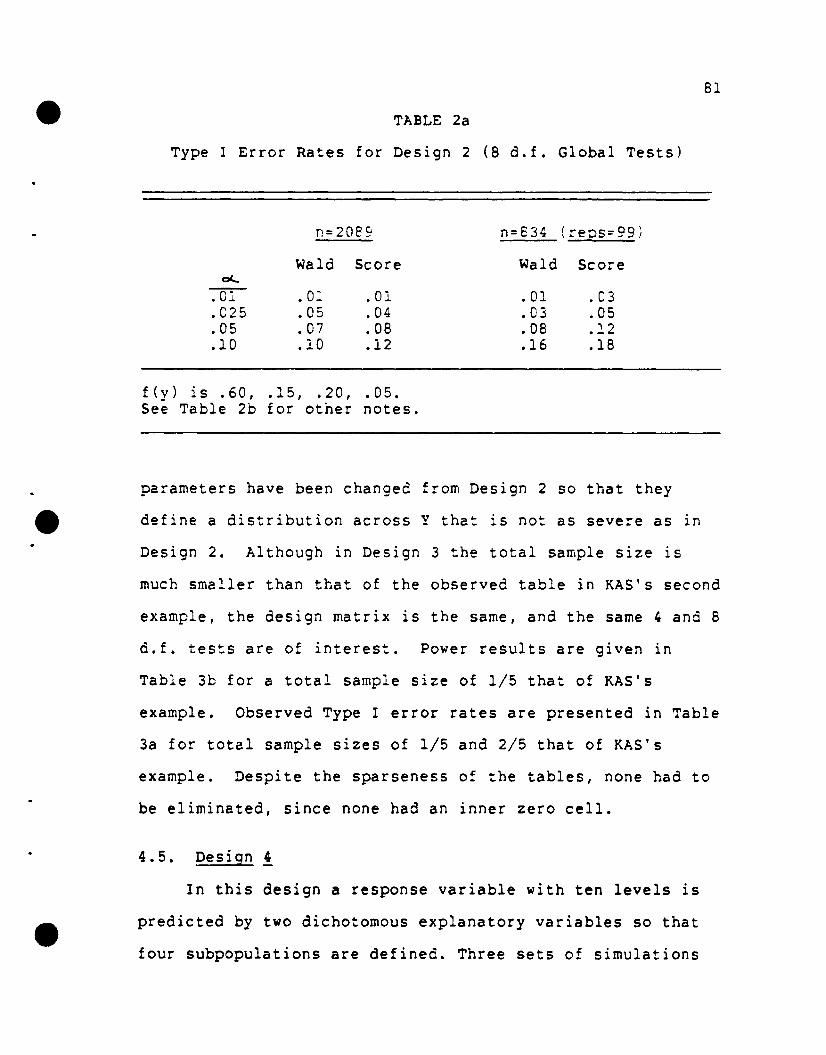
81

TABLE 2a

Type I Error Rates for Design 2 (8 d.f. Global Tests)

n=208S' n=834 (reos=99)

Wald Score Wald Score0(..

:D"l .01 .01 .01 .03.C25 .05 .04 .03 .05.05 .07 .08 .08 .12.10 .10 .12 .16 .18

f (y ) is . 60, .15, .20, . 05 .See Table 2b for other notes.

parameters have been changed from Design 2 so that they

define a distribution across Y that is not as severe as ln

Design 2. Although in Design 3 the total sample size is

much smaller than that of the observed table in KAS's second

example, the design matrix is the same, and the same 4 and 8

d.f. tests are of interest. Power results are given in

Table 3b for a total sample size of 1/5 that of KAS's

example. Observed Type I error rates are presented in Table

3a for total sample sizes of 1/5 and 2/5 that of KAS's

example. Despite the sparseness of the tables, none had to

be eliminated, since none had an inner zero cell.

4.5. Design 4

In this design a response variable with ten levels is

predicted by two dichotomous explanatory variables so that

four subpopulations are defined. Three sets of simulations

82

TABLE 2b

Powers for Design 2

n=20898 d. f. 4 d. f.

Wald Score Wale Score0<.

:or- .16 .29 .31 .43.025 .29 .42 .42 .59.05 .40 .51 .54 .71.10 .47 .61 .69 .83

n=8348 e.. f. 4 • &c . .l. •

Wald Score Wale. Score0<.

:or- .08 .11 .09 .12.025 .09 .12 .10 .20.05 .12 .23 .18 .31 e.10 .19 .31 .26 .44

k=3: p=4:~= -2.082, -2.867, -5.027:l = (-.037 .860 .428 1.830)':'tjl for S51 = -. 39, . 83 :ljJ for S52 = -. 07, 1. 20 :

The n~ are either as in the KA5paper or 2/5 that size.

f(y) is .60, .16, .12, .12.

Design matrix has dummycoded vectors for (inthis order) AP, JE, 551,and 552.

are run in which only the ~jL parameters are different. In

the first simulation all lj~ parameters are zero. In the

second simulation the ~l associated with the lowest and

highest values of Yare larger than the ~j.l. associated with

the middle values of Y, and in the third simulation the

parameters are more or less of uniform size across·the

83

TABLE 3a

Type I Error Rates for Design 3 (8 d.f. Global Tests)

n=417

Wald Score

n=834

Wald Score0<.­

:or­.025.05.10

.01

.04

.08

.14

.02

.04

.09

.15

.00

.04

.04

.08

• C2.02.06.13

f(y) is .07, .14, .25, .53.See Table 3b for other notes.

levels of Y. The subpopulation sizes and the regression

parameters are chosen so that some sparseness in the cells

is evident, especially for the smallest and largest values

of Y. Results are given in Table 4 for the 16 d.f. global

tests. Three of the tables from the second simulation had

to be eliminated.

4.6. Design 5

In this design the sparse cell situation is

deliberately avoided: all cells uniquely defined by a level

of Y and a level on one of the explanatory va~iables have

substantial sample sizes. A four-level dependent variable

is predicted by five completely crossed dichotomous

predictor variables so that 32 subpopulations are defined.

All n' =.. 10 so that n = 320. Three sets of simulations are

run that differ only in their ~j.t parameters. In the first

84

TABLE 3b

Powers for Design 3

Mo6era~elv laroe rj~

8 d. f. test 4 d. f. test

Wald Score Wald Score~

.01 .44 .66 .57 .72

.025 .60 .74 .75 .79

.05 .76 .82 .82 .87

.10 .83 .88 .91 .90

4 6.. f. ~est, Smaller tjl

Wald Score0<-

.01 .18 .25

.025 .29 .36

.05 .43 .49

.10 .51 .54

k=3: p=4:"j =1 . 39, 0, -1. 39:t = (-.037 .860 .428 1.830)'.

The n~ are 1/5 the size ofthose in Ex. 2 of the KASpaper; n=417.

Design matrix is thesame as in Table 2b.

La rger J,;1. are 3/4 thesize of those in Table2b; smaller are 1/2those in Table 2b.

f (y) for 1a r ge r 'tjJ is. 07, •15 , •11, •66:f (Y) for sma11e r rj.l is. 07, •15 , •15 , • 62 •

simulation all five predictor variables have proportional

odds; in the second all five variables have nonproportional

odds, although the pattern of nonproportional odds is

different for each variable. In the third simulation only

the fifth predictor variable has nonproportional odds; the

pattern of nonproportional odds for this variable is chosen

85

TABLE 4

Type I Errors and Powers for Design 4 (Global Test)

h' - 'tjJ = 0J.J.

Wald Score0<.

:or .00 .01.025 .00 .03.05 .01 .04.10 .04 .10

The ~. are ouite variable (Reps=97)

Wald Score

:or.025.05.10

.21

.28

.38

.52

.31

.41

.53

.69

The 'l/jt. are re1a t i ve 1y homogeneous

Wald Scorec;>(....

:or­.025.05.10

.11

.19

.27

.38

.17

.27

.31

.48

.08, .05;

.08, .05;

.11, .04.

simulations are:.14, .15, .17, .12,.12, .19, .14, .13,.16, .15, .17, .10,

the three.08, .13,.07, .14,.10, .10,

k=9; p=2;All n4 =100; n=400;~j= 3.18,2.20,1.39,.62,0,-.62,-1.39,-2.20,-3.18;i= (.3 .3)'.The f(y) for

.03, .04,

.03, .05,

.03, .03,

86

to be the same as in the first simulation. In the latter

two simulations, six test statistics are compared: the 10

d.f. global statistics and the five individual 2 d.f.

statistics. In the fi~st simulatio~ o~ly the 10 d.f. globa:

statistics are compared. Results are given in Table 5.

Since the first four predictor va~iables in the third

simulation have proportional odds, the corresponding entries

in Table 5 are observed Type I error rates for the 2 d.f.

statistics.

Compared to the designs considered previously, this

design shows ve~y little diffe~ence in power between the

Wald and score statistics. This is particularly surprising

for the test of proportional odds for the fifth explanatory

variable in the third simulation. Here the other four

predictor variables have proportional odds, so it would seem

that the score test would be at an advantage. That is, the

score statistic is calculated under the assumption that the

other four variables have proportional odds, whereas the

Wald statistic is not. An equally surprising result is that

the power of the Wald statistic for the fifth explanatory

variable in the third simulation is slightly larger than its

power in the second simulation where all five variables have

nonproportional odds.

4.7. Design 6

In this design, as in the previous design, five

completely crossed dichotomous predictor variables are used

to predict a four-level response variable, but in this

•

TABLE 5

Type I Errors and Powers for Design 5

Global Test, all ~jr = 0

Wald ScoreC"C-.

• 01 .C2 .03.025 .05 .07.05 .07 .09.10 .09 .14

87

Five oredictor variables have nonprooortional odds

Wald/Score

Global Xl X2 X3 X4 X50<-

:or .52/.59 .07/.06 .14/.15 .08/.10 .12/.11 .36/.41.025 .68/.70 .13/.15 .20/.23 .18/.20 .19/.20 .53/.57.05 .79/.79 .20/.19 .34/.34 .24/.29 .28/.27 .66/.67.10 .85/.85 .26/.27 .42/.42 .36/.37 .42/.37 .73/.73

Only fifth variable has nonproportional odds

Wald/Score

Global Xl X2 X3 X4 X50<...

:or .16/.21 .00/.00 .01/.01 .00/.00 .00/.01 .41/.45.025 .32/.34 .01/.01 .02/.02 .02/.02 .02/.03 .59/.60.05 .42/.46 .02/.03 .04/.05 .08/.07 .05/.06 .72/.76.10 .56/.62 .08/.05 .06/.07 .09/.10 .10/.12 .85/.84

k=3; p=5;o(~ = .405, -.847, - 2.20 ;~= {.5 .5 .5 .5 .5}'.

All n~=10; n=320.

The f{y} for the 3 simulations are:.17, .23, .30, .29:.17, .23, .39, .21:.17, .18, .35, .29.

Xl: -.3, -.5X2: -.4, -.4X3: .3, .5X4: 0, -.5X5: .5, 0

88

design the regression coefficients are chosen so as to

provoke the sparse cell problem. In particular, the ~~ are

identical to those used in the first (null) and second (non­

null) simulations of Design 5, but all the ~J and B~

parameters are much smaller. The net result is that for

both the null and non-null simulations very few observations

in any subpopulation have Y=3. In fact, summed a:ross all

subpopulations, the larger the value of Y, the smaller the

sample size. The Type I error rates for total sample sizes

of 320 ana 640 given in Table 6 show that the score teSt is

performing poorly, probably due to the sparse sample size at

Y=3. Powers for n=320 are also given in Table 6, where it

can be seen that the difference in power between the 10 d.f.

Wald and score global tests is larger than it is in the

second simulation in Design 5. For example, for a Type I

error rate of .05, powers of .40 and .58 for the Wald and

score tests, respectively, are obtained in Design 6, whereas

powers of .66 and .67 are obtained in the previous design.

Whether the extreme marginal distribution of Y causes the

score test to have more power than the Wald statistic cannot

be ascertained from this simulation alone, but there seems

to be some evidence that it does, since the score statistic

overestimates the Type I error rates.

4.8. Design 2

The simulations for this design are based on the third

example in the KAS paper, a clinical trial with 235 patients

that compares an active treatment with a placebo. Twelve

,

89

TABLE 6

Type I Errors and Powers for Design 6

Globa: Tes:, a:: lit =0

n=320 n=640

Walo Sco:-e Wald Score0(.

.01 .00 .06 .00 .03

.025 .02 .Oi .04 .07

.05 .03 .09 .04 .10

.10 .09 .16 .12 .20

All five variables have nono:-ooor'tional oads (n=320)

Wald/Score

Global Xl X2 X3 X4 X5oc.

:or .18/.35 .02/.04 .06/.09 .04/.06 .00/.03 .16/.20.025 .31/.48 .04/.06 .15/.18 .06/.11 .00/.06 .25/.30.05 .40/.58 .07/.08 .25/.28 .11/.18 .03/.13 .38/.41.10 .53/.71 .14/.18 .33/.34 .26/.31 .14/.22 .55/.59

k=3: p=5:01..;= -.85, -2.20, -3.90:~= (.2 .2 .2 .2 .2)';

All n.=n/32.f(y) for null case: .59,f(y) for non-null case:

All l~t as in Table 5.

.26, .12, .03.

.59, .24, .15, .02.

subpopulations are defined by six investigators and two

treatment groups, so that the design matrix has five dummy­

coded vectors defining investigator and one vector defining

treatment. A three-level ordinal response variable

indicates cure-status: cured at 2 weeks, cured at 4 weeks

but not at 2 weeks, or not cured by 4 weeks. Previously it

was mentioned that in this simulation many of the Wald and

90

score statistics are unrealistically large because of inner

zero cells. This is largely due to one investigator who has

only 7 patients under the active treatment and only 10 under

the placebo.

When used on KAS's observed table, the 6 d.f. global

Wald test of proportional odds has an approximate chi-square

value of 11.332 (p=.079), whereas the score test has a value

of 13.26 (p=.039). The five d.f. Walo test of proportional

odds for the investigator effect gives Q~= 11.06 (p=.050),

whereas the comparable score test gives R = 12.56 (p=.028).

Both of the 1 d.f. tests of proportional oods for the

treatment effect are quite small (Q,=.14 and R=.26). As a

consequence of these results, a non-null simulation allows

only the treatment effect to have proportional odds, and all

regression coefficients used in this simulation are set

equal to those estimates produced when the ML procedure is

used on KAS's observed table, with only investigator being

fitted for nonproportional odds. Another simulation uses

the same ~j and ~ parameters as in the first simulation,

but all the r~ parameters are set to zero.

Since many statistics in both of these simulations were

obviously too large, this design was used to study the

performance of the modified score statistic. The likelihood

ratio statistic was calculated as a standard by which to

compare the other statistics, but, surprisingly, this

statistic, which was previously thought ~o perform quite

-well, does not preserve the nominal Type I error rate.

•

•

•

•

•

91

Table 7a gives the observed rates for the likelihood ratio

test, the Wald test, and the modified and original score

tests for three situations: when all 100 replications are

usee, wher only rep:ica:ions with no inner zero ce:ls are

used, and when only replications with no inner or outer zero

cells are used. As mentioned before, this Table shows that

eliminatins f:equency tables with inner zero cells is

sufficient to allow all four test statistics to preserve the

nominal Type I error rate. The Table also shows that the

modified and original score tests seem to perform equally

well, once these problem tables are eliminated.

Table 7b gives power estimates for the Wald, score, and

likelihood ratio tests under the same three situations as in

the null case. These results were discussed in some detail

in section 3.4.

4.9. Desion 8

This design follows from KAS's fourth example, a

randomized clinical trial comparing an active treatment with

a placebo (n=193). The five-level ordinal response variable

categorizes pain condition as either poor, fair, moderate,

good, or excellent. Sixteen subpopulations are defined by

the cross-classification of four types of diagnostic status,

two investigators, and two treatments.

Analysis of the observed table presented in the paper

gives 15 d.f. global tests of Qt= 35.02 and R • 46.22, bothN

significant. Tests for each of the three effects separately

give nonsignificant 9 d.f. tests for diagnostic status,

92

TABLE 7a

Type I Error Rates for Design 7 (Global Tests)

•

All 100 Reo~ications ..Modified

Wald Score Score L.R.0<.

.01 .23 .24 .08 .17

.025 .24 .26 .10 .17

.05 .26 .29 .15 .22

.10 .27 .31 .17 .31

Reolications deleted if inner zero cell (Reps=73)

0<.

:ar- .027 .027 .027 .027.025 .041 .055 .041 .027.05 .068 .062 .062 .082.1(1' .082 .123 .123 .151 •

Replications deleted i f an\, cell = 0 (Reos=46) e~

,

:ar- .043 .022 .022 .022.025 .065 .043 .043 .022.05 .065 .065 .065 .065.10 .087 .065 .065 .087

f(y) is .39, .17, .42.See Table 7b for other notes.

...

TABLE 7b

Powers for Design 7 (Global Tests)

),1::- 100 Rep1ica:ions

ModifiedWald Score Sco:-e L.R.

0<.

:or- .4i .36 .55 .42.025 .56 .52 .65 .55.05 .65 .61 .74 .66.10 .74 .70 .80 .74

Reolications deleted if inner ze:-o cell (ReDs=69)

0<..

:or- .30~ .333 .420 .232.025 .420 .4i8 .551 .420.05 .551 .609 .681 .580

.. .10 .681 .696 .754 .700

e Reolications deleted if any cell = 0 (Reps=46)

~

:or- .391 .370 .522 .261.025 .543 .590 .652 .478.05 .674 .652 .761 .652.10 .804 .739 .826 .739

93

k=2: p=3:eCj =- 1 . 48, - 2 • 31 :t = (2.05 2.00 3.98 2.77 1.70 -.53):rjl for investigator effects ...

-1.99, -.69, -172, -1.34,-.71;The n: are as in the KAS paper: n=235.£(y) is .39, .40, .20.

Design matrix has5 dummy codedvectors forinvestigator and1 for treatment.

94

nonsignificant 3 d.f. tests for treatment, and significant 3

d.f. tests (Qc = 22.98 and R = 33.76) for investigator. As

a conseguen:e of these results. a no~-null simulation allo~5

only investigato: tc have nonproportional odds. The

regression coefficients used in the simulation were

initially set equal to those estimates produced when the ML

procedure was usee on the observed table. Since these

coefficients gave powers of almost 1, the coefficients

eventually used were half this size. A null case simulation

~as also run which used the same ~d and ~L parameters, but

the 1jl were set to zero.

Since both the Wald and score tests behaved so poorly

in the null case, this design was used to study the modified

score statistic. Results for both simulations, given in

Table 8, were discussed in some detail in section 3.4.

Because the probability that Y=l is small (.04) in the null

simulation, Type I error rates for both the original and

modified score test are too large. Powers, based on 84

tables not eliminated due to inner zero cells, are probably

less subject to invalid statistics, since the marginal

distribution of Y is more uniform.

4.10. Design ~

In this design a 4-level response variable is

predicted by a "pseudo-continuous" explanatory variable.

This explanatory variable has 10 values ranging from 0 to 9

with the same number of observations at each value. Four

sets of simulations are presented: null and non-null

Design matrix has3 vectors for diagnosis,1 for investigator,and 1 for treatment.

95

TABLE 8

Type I Error Rates and Powers for Design 8 (Global Test)

All toi, = (1, 100 Rep1 i cat ion s

Modified'Wald Score Score

0<-

-:D'l .11 .65 .66.025 1 1 .65 .66.--.05 .15 .72 .73.10 .21 .74 .76

All tjf = o, Replications deleted if inner zero cell(Reps = 36)

Modified'Wald Score Score

-<-:or- 0 0 0.025 0 .105 .105.05 0 .289 .289.10 .053 .368 .368

All ~jl =O. Replications deleted if inner zero cell(Reps = 84)

Modified'Wald Score Score

C'<.-:or- .24 .44 .44.025 • 2-7 .52 .52.05 .40 .65 .65.10 .60 .80 .80

k=4: p=5:lX,)' = -. 23, -. 45, -1. 16, - 3.16 :t = (1.25 .75 .03 1.36 .52)':~L for investigator are

-.62, -.48, -.30.The ~are as in the KAS paper: n=193.f(y) for null case is .25, .04, .14, .38, .19.f{y) for non-null case is .25, .10, .14, .35, .16.

96

simulations with total sample sizes of either 200 or 300.

The results in Table 9 show that both tests seem to maintain

the nominal Type! error rate a little better for the larger

sample size. Nc diffe~ences lr. powe~s are apparent.

2.11. Desion 10

This is the only design in which the test of a linear

constraint is examined. Ins:ead of using the Wale sta:is:ic

from the FARM procedure, statistic (12) described in Chapter

2 is used. Recall that this statistic is a test of the

goodness of fit of the mode~ described

= Z1--The comparable score statistic is described on page 46 of

Chapter 2. The particular design considered here has a

five-level response variable and one dichotomous explanatory

variable. For this situation, the FARM procedure tests the

goodness of the weighted least squares fit of the f02lowing

model (using FARM procedure notation):

•

TABLE 9

Type I Errors and Powers for Design 9

97

Non-null

Non-null

n=200Null

Wald Scoreex

~ .0:3 .03.025 .04 .03.05 .07 .08.10 .14 .16

n=300Null

Wald Score0<-

:ol .00 .00... .025 .00 .01

e .05 .05 .04.10 .08 .08

Wald

.18

.25

.36

.46

Wald

.30

.41

.51

.57

Score

.20-~• L. I

.38

.46

Score

.29

.42

.52

.59

Design matrix has one"continuous" variablewith 10 values.

k=3; p=l;"".j = 1.1,0,-1.1;e. - - 03'- . ,t~ = •05 , • 1 0 ;all n~ = n/lO.fey) for null case is .28, .26, .24, .23;fey) for non-null case is .28, .20, .21, .31.

....E ( P) =.. z

100 0 0 00000' 0o 1 0 C C Go 0 00: J.001 CJ 0 000001 2o 0 0 1 0 0o 0 0 013

-98

Both this test and the comparable score test have 2 d.f.

Three simulations differing in sample size and ln their

se lee t ion 0 f the ~.it. pa rame t e r suse t his des i gn . Us i ng P =

.1 (ML procedure notation), two null case simulations with

sample sizes of 120 and 240 have ~1 parameters of. 1, .2,

and .3, so that the log odds ratios for the four cumulative

probabilities are linear: .1, .2, .3, and .4. Another

simulation uses a sample size of 120 and ~.i.l parameters of

.4, .7, and .1, while a fourth simulation uses this same

sample size and the parameters 1.0, .4, and .7. Results are

given in Table 10.

4.12. Summary of Simulation Results

Results from the null case simulations and all

simulations in Tables 7b and 8 are discussed in some detail

in section 3.4 where these simulations are used to study

invalidity in the score and Wald tests. Although both tests

are anti-conservative when the frequency tables contain

inner zero cells, only the score test appears to have

..

•

TABLE 10

Type I Errors and Powers for Design 10

~J..l = .1, .2, .3

99

0<...:Dl.025.05.10

Wala

.01

.03

.05

.08

n=120

Score

.03

.05

.09

.12

Wald

.01

.03

.04

.07

n=240

Score

.02

.03

.04

.09

~j~ = .4, .7, .1, n=120

Wala Score0(.

:or .12 .23.025 .19 .27.05 .27 .34.10 .36 .44

tJ.t = 1, .4, .7, n=120

Wa1d Score~

:or- .64 .86.025 .77 .90.05 .83 .91.10 .86 .93

k=4; p=l:~=.69, -.34, -1.61, -2.4:!. = .1; n = n/2.The f(y) for the 3 simulations are:

.32, .24, .25, .08, .10:

.32, .20, .24, .15, .09;

.32, .13, .34, .08, .13.

Design matrix hadone dichotomousvariable.

100

problems when the marginal distribution of Y is markedly

non-uniform. In particular, if, relative to k, any of the

marginal percentages of Yare small, then the score test

appears to be anti-conservative. Thus, a marginal percen:

of .03 when k=3 causes a problem for the design in Table 6,

but this same percentage when k=9 is no problem for the

design in Table 4. Doubling the sample size in Table 6 does

not improve the Type I error rates. Both tests have a

slight tendency to overestimate the Type I error rates for

the simulations in Tables la, 2a, 3a, and 9, although

increasing the sample size appears to improve these

estimates. Since the tables in these simulations have no

immer zero cells and have less problematic marginal

distributions of Y, this result was interpreted to imply

that some other source of ill-conditioning might exist,

perhaps a general sparseness of cell sizes.

For the score test only, the null case simulations from

Tables 5 and 10 show Type I error rates that are slightly

larger than expected, even though the frequency tables

appear "good." When the sample size is doubled in the

simulation in Table 10, the observed Type I error rates are

improved. This suggests that such an increase in sample

size might also improve the estimates in Table 5.

Since both test statistics seem to have problems with

sparse cells, and the score test, in addition, has a problem

with the marginal distribution of Y, power results should be

approached with caution. For example, the powers in Table 6

101

are based on a simulation scenario where Y has four possible

values, but only 2% of the observations fall in the highest

value. ~he comparable null case simulation has only 3% of

its obse~va:ions at this value, anc the s=ore test canno:

maintain the Type I error rate. Therefore, the powers in

this Table may be incorrect. However, the powers in other

Tables are probably more trustworty, since the marginal

distributions of Yare not as extreme and since the Type 1

error rates are more reasonable. The use of the observed

Type 1 error rates in judging the validity of the powers is,

however, of uncertain relevance, since, as mentioned in

section 3.4, the difference between the null and non-null

cases is more complex than in, say, the simple t test. For

example, in Table 1 the Wald and score tests both give the

same observed Type I error rate of .02 for the nominal rate

of .01. At the nominal rate of .05, however, the Wald test

correctly gives .05, while the score test gives .10.

Nevertheless, the powers in this situation show the biggest

difference between the two statistics at the nominal rate of

.01 (Wald has .49, score .66) and the smallest difference at

.05 (Wald .78, score .82). This seems counterintuitive,

since one would expect the greatest difference in powers to

occur at the greatest difference in Type I error rates.

Table 2a shows that the Type I error rates for both

tests look better for a sample of size 2089 than for a

sample of size 834, especially for the score test. The

comparable powers in Table 20 ~how that for both sample

102

sizes the score test has considerably more power than the

Wald test. For this design the marginal probability that

Y=3 is .05 in the null case simulation, while in the non­

null simula~ion all marginal probabili~ies are at leas: .:2.

These results suggest that even if the tests cannot maintair.

the Type! error rate, the powers may not be distorted.

The difference in power be:ween the Wald ana score

statistics depends upon the simulation and the nominal Type

I error rate. For example, Tables 2b, 4, 8, and 10 display

rather large differences in power (.10-.25), whereas Tables

5 and 9 show quite small, insignificant differences. Tables

1, 3b, and 10 show cases where the smaller the nominal Type

I error rate, the larger the power differences, while other

Tables such as 2b, 4, and 8 show no such result.

Use of these simulations to characterize those

situations that cause the greatest difference in power may

lead to overinterpretation of the data. The problem is

obvious: this paper can present only a few simulations

based on only a few of the many possible designs.

Nevertheless, if a guess must be ventured, it does appear

that the difference in power is somehow related to cell

sizes. That is, in general, simulations that use tables

with sparse cells show larger differences in power than do

simulations that use tables with less sparse cells. Table

5, for example, shows very small differences in power, and

here sparse cells are rare. Table 8, OM the other hand,

. shows very large differences in power (.20 or larger), and

103

the sparse cell problem is so severe that 14 tables had to

be eliminated due to inner zero cells. By the way, the

distribution of Y for this latter simulation has no small

percentages that coule be contributins tc this resu~t.

Table 9 displays Type I error rates and powers for the

only design using a continuous predictor variable and thus

the only design in which references to sparse cells are

irrelevant. The design here has k=3 and a rather uniform­

looking marginal distribution of Y in the null and non-null

simulations. The powers for the Wale and score tests are

almost identical for total sample sizes of both 200 and 300.

For both the Wald and score statistics, the Type I error

rates are improved when the sample size is increased from

200 to 300. This latter result, seen also in several Tables

that use categorical predictor variables, suggests that

sparseness of cell sizes may not be the only cause of

inflated Type I error rates, but that the total sample size

may also be important. Whether the powers of the two teSt

statistics are similar because the predictor variable is

continuous instead of categorical cannot be determined from

this one simulation.

CHAPTER V

A DATA ANALYSIS STRATEGY

5.1 Introduction

This chapter describes an approach for fitting the

{constrained} partial proportional odds model described in

this paper. The approach is illustrated by using as an

example the p~ediction of cardiovascular disease from a set

of standard risk factors such as age and smoking status.

Since the current ML program has the limitations detailed in

section 2.5.4, the analyst may not always be able to fit the

most appropriate model, and thus the example illustrates how

the analyst must work within these limitations.

Graphical methods for assessing proportional odds are

also described in this chapter. These methods can help the

analyst decide what type of constraint, if any, should be

applied across the k log odds ratios associated with each

predictor variable in the model. The graphical methods are

described first, using two predictors of cardiovascular

disease as examples.

5.2. Graphical Methods for Assessing Prooortional Odds

One way to graphically assess the assumption of

proportional odds for the relationship between an ordinal

response variable and a dichotomous predictor variable is to

105

consider the k possible log odds ratios arising from the k

possible dichotomizations of Y: Y~j vs. Y<j, j=1, ... ,k.

These log odds ratios and their con~idence intervals, ~hen

plo:tec against j, car. assist the ana2ys: in assessing

proportional odds. Specifically, if the relationship

between a dichotomous ?redictor variable X and the jth

dichotom:~a:ion of a response variable Y is represented by

the 2x2 crosstabulation table

X1 0

+-----+-----+Y~j I a I b I+-----+-----+Y<j I c I d I+-----+-----+

then the log odds ratio is log(ad/bc) and its Taylor series

confidence interval is:

z\_.~ is the value of a standard normal variate, Z, such that

pr(Z > Z,-oI,J2.) = oC/2 (Kleinbaum and Kupper, 1982).

A simple SAS macro to calculate and plot the above

statistics is given in Appendix 3; in this macro ZI-CIl./~ is

currently set at 1.96 so that 95% confidence intervals are

calculated. As an example of the results from this program,

in Figure 1 is a plot of the relationship between severity

of cardiovascular disease (CAD) and smoking status (SMK) in

the Duke dataset discussed in section 2.4. Here the

response variable has six levels, and the predictor

Figure 1

Odds Ratios for Relationship BetweenCardiovascular Disease and Smoking Status

106

J OR LOGOR LOWER UPPER

1 3.45865 1.24088 1.00820 1.473562 2.67925 0.98554 0.77777 1.193313 1.86331 0.633C3 0.~3723 0.828834 1.55676 0.44389 0.23500 0.652785 0.98660 -0.01349 -0.36609 0.33912

P:"OT OF LOGOR*JPLOT OF LOWER*JP:"OT OF UPPER*J

LOGOR

1.5 +

1. 0 +

0.5 +

0.0 +

-0.5 +

SYMBOL USED IS *SYMBOL USED IS +SYMBOL USED IS +

+

* + e+ *

++

* +

*+ +

+

*

+

I---+-------+-------+-------+-------+-------+--

o 1 2

J

3 4 5

107

variable, smoking status, is dichotomous. In the plot the

vertical axis gives the log odds ratios and the horizontal

axis gives j, the point of dichotomization of the disease

variable. The values of a:l plotteD points are given

directly above the plot. The figure shows that the

relationship between cardiovascular disease and smoking

s~atus does not fit the proportional odds assumption. In

particular, notice that as j increases the log odds ratio

decreases, and that, in fact, this relationship appears to

be linear. Thus, the analyst will probably want to test the

goodness of fit of a linear constraint.

If a predictor variable is continuous and a plot

similar to the one in Figure 1 is wanted, then one

alternative is to dichotomize this continuous variable and

use the SAS macro described above. Figure 2, for example,

shows the relationship between cardiovascular disease and

duration of symptoms (actually, log,o of duration of

symptoms, CAD_DUR) where duration has been dichotomized

around its observed median. The plot shows that the

relationship does not fit the assumption of proportional

odds. Notice in this plot that there appears to be no

relationship between disease and duration of symptoms until

j is at least 3, i.e., the log odds ratios at j = 1 and 2

are not significantly different from zero. The reason for

this rather surprising result is that the dataset contains

many patients with no disease (Y=O) or insignificant disease

(Y=l) who have nevertheless been complaining of symptoms for

lOB

Figure 2

Odds Ratios for the Relationship BetweenCardiovascular Disease and Duration of Symptoms,

Dichotomized at the Mediar.

J OR LOGOR LOWER UPPER

, 1.23152 0.208246 -0.018964 0.'35461...2 1.15261 C.l'2205 -0.057898 0.3423093 1.77687 0.574855 0.390730 0.7589804 1.81511 0.596148 0.402929 0.7893675 1.75975 0.565170 0.220294 0.910047

PLOT OF LOGOR*J SYMBOL USED IS '"PLDT OF LOWER*J SYMBOL USED IS ~

PLOT OF UPPER'i<"J SYMBO:' USED IS •

LOGOR +

+0.75 + e

'"* *

0.50 ++

+ ++

0.25 + +

**

0.00 + ++

-0.25 +---+-------+-------+-------+-------+-------+--

a 1 2

J

3 5

109

years. These patients are either hypochondriacs or have

heart problems unrelated to coronary artery disease. The

plo: indicates that a linear constraint will probably not

fit this relationship, al~hougn a more appropriate

constraint will be discussed in the next section.

If the predictor variable is continuous and the analyst

does not want to artificially dichotomize, then ano~her more

expensive plotting strategy is possible. That is, each of

the k possible dichotomizations of Y can be separately

regressed on the predictor variable, resulting in k maximum

likelihood analyses. From each of these regressions is~

obtained a ~, which is the log oads ratio, and its standardA A

error, Var(p). These statistics can then be plotted and

interpreted in the same way as statistics resulting from an

artificial dichotomization. As an example, Figure 3 gives

such a plot for the CAD/CAD DUR relationship. A comparison

of Figures 2 and 3 shows that the plots lead to very similar

assessments of the relationship between duration of symptoms

and CAD.

The technique just described for producing plots

involving continuous predictor variables can also be used

when the analyst wants to examine the proportional odds

assumption for one predictor variable while controlling for

one or more covariates. Thus, the k maximum likelihood

analyses simply contain covariates as well as the predictor

variable being studied for proportional odds. As before,

·the regression coefficient, ~, associated with the predictor

Figure 3

Odds Ratios for the Relationship BetweenCardiovascular Disease and Duration of Symptoms

(Odds Ratios Estimated by Maximum Likelihood)

110

J OR LOGOR LOWER UPPER

1 1.28403 0.25 0.0540 0.44602 1.27125 0.24 0.0636 0.4:'643 1.89648 0.64 0.4636 0.816~

4 1.99372 0.69 0.5136 0.86645 2.41090 0.88 0.4488 1.3112

PLOT OF LOGOR*J SYMBOL USED 1S *PLOT OF UPPER*J SYMBOL USED IS +PLOT OF LOWER*J SYMBOL USED IS +

1. 50 +

+ e1.25 +

1.00 +

LOGOR + *+

0.75 +

**

0.50 + ++ + + +

0.25 + * *

+ +0.00 +

---+-------+-------+-------+-------+-------+--o 1 2

J

3 4 5

111

variable of interest is the log odds ratio to be plotted.

In all the plots described above, the k possible log

odds ratios are plottec against j, the point of

dichotomization of Y. These plo:s give the analyst a ve~y

good visual impression of whether the proportional odds

assumption is met. They are also useful in assessing what

:ype of constraint can be imposed across the k log odds

ratios. However, there is another entirely different type

of plot which can be useful in assessing proportional odds

when the predictor variable, X, is continuous. That is, for

each J, j=l, ... ,k, the logit of the proportion of Y~j is

plotted against X, so that k probability curves appear on

the same plot. As an example, such a plot for the

CAD/CAD DUR relationship is given in Figure 4. If the jth

regression line on such a plot is given by

log i t [ Pr (Y~ j I X») = o(j + 6j X,

then proportional odds implies that

=

10git[Pr(Y~j IX=x») - 10git[Pr(Y~j' IX=x»)

oCj - j'" + (~j - ~';/) X

is independent of X. This can occur only if ~~ = ~J'. Thus,

proportional odds is equivalent to the k regression lines

being parallel. In Figure 4 for example, proportional odds

appears not to hold since the lines are further apart at the

low values of j than they are at the higher values of j.

Such an assessment is, however, hampered by the lack of

Figure 4

Proportions of CAD>=j (j=1-5) vs. CADDURCADDUR Crouped Into f 0 Quantile Croups

2.52.01.51.00.5

/~, /~-~--AIt- /' .,,/___~ _--~---r--

+- ' .............; "'..__-+----+-~~t •

)f-- ...... '

__ u __u_...- " - ,.. __ ----M--_.... ,..' -----KK-------K "----- ",--- --~ .....--"")f--- .... --..------

/~, ////

........ ... ---- ---.-------~ ~--- ---~-

1.0

0.9

0.8

0.7

0.6-i>i 0.5

0.4­

0.3

0.2

0.1 I

o 0 1 +---- ~~---.----+--. - ---+---.• I"""" ,----.- --.,_.t"'" ·I-'·'i""

00'"·'''''''1'''''''''

• I

CADDURI-'I-'IV

e e.•e

113

confidence intervals, although such intervals could be

calculated. Nevertheless, even with confidence intervals,

the plot would not be helpful in finding a good constraint

tc: fit :'he data, i.e., the plo: does not immediiOtely sU9ges:

good ~ values to be used in the constrained partial

proportional odds model.

5.3. A Data Analysis Strategy

In this section an approach to fitting a partial

proportional odds model is suggested that appears to work

well on the aatasets considered so far. Certainly, other

approaches are possible, and the analyst may want to tryout

his or her own ideas for building a model. The approach to

data analysis outlined below takes the limitations of the

current computer program into account, while at the same

time revealing the ideal analysis strategy. The step-by­

step outline below will be followed by an example that

illustrates its application to a real dataset.

Step 1. Build a proportional odds model using a

recommended procedure, for example the forward selection

procedure or backward elimination procedure described by

Kleinbaum and Kupper (1982). The resulting model will

contain, in addition to main effects, "significant"

interaction terms and "significant" quadratic or cubic terms

involving continuous predictors.

Step 2. Use a graphical procedure described in the

previous section on all main effects selected into the model

in step 1. Examination of the resulting plots will help the

114

analyst interpret the results from Step 3.

Step 3. Using the final model developed in Step 1,

calculate k-l d.f. score tests of proportional odds for all

ma:~ effects, or at least for :hose main e:fec:s whose plo:s

in Step 2 suggest nonproportional odds. Since the

relationship among the k log odds ratios seems frequently to

be linear, a 1 c.f. score test of a linear constraint ror

each of the main effects might also be performed at this

time. Obviously, however, the analyst is free to test any

constraint she wishes, or to test none at all. If both the

k-l d.f. score test and the 1 d.f. test of a constraint are

significant, the k-2 d.f. score test for the goodness of fit

of the constraint should be examined. If this k-2 d.f. test

is nonsignificant at some preset level, indicating that the

constraint fits the data, the analyst will want to fit this

constraint to the predictor variable. If no simple

constraint can be found to fit a variable having

nonproportional odds, then all k-l ~k parameters will have

to be used in the model.

Step 4. Fit the {constrained} partial proportional

odds model suggested by the score tests in Step 3.

Unfortunately, at the present time if the analyst wants to

fit a constraint to anyone of the predictor variables

having nonproportional odds, the same constraint must be

used on all q. of these variables. Although admittedly

limiting, this is the only strategm possible with the

. present software. Thus, the analyst must try to find a

•

115

constraint that fits all q, variables at least modestly.

If it is impossible to fit a common constraint to the

~ variables, the analyst has two options. One, she may

simply fit an unconst~aineo pa~tigl propo~tional od6s mODel,

realizing, of course, that the model degrees of freedom may

increase drama~ically. This option is, therefore, probably

only feasible if both q, and k are small. The second optior.

is to ignore the nonproportionality of one or more of the q.

va~iables and fit a common constraint to the remaining

variables. The resulting model will not be optimal, but it

will certainly be better than the strict proportional odds

model which had been the only ML model generally available

up until now that used the ordinality of the dependent

variable.

Step 5. When fitting the model in step 4 above, the ML

program also simultaneously allows the analyst to obtain two

types of score tests. For those variables with a

constrained ~ term in the model, a k-2 d.f. score test of

the goodness of fit of the constraint can be obtained. In

Step 3 a similar statistic was obtained by taking the

"difference between a k-l d.f. score statistic and a 1 d.f.

score statistic. The analogous statistic obtained here in

Step 5, however, is the better statistic, as was explained

in section 2.5.3. Recognize, nevertheless, that a large

disparity between these two goodness of fit statistics may

simply be due to the fact that they are calculated in the

presence of two entirely different models. That is, in Step

116

3 the tests are calculated in the presence of a proportional ~.

odds model, whereas in Step 5 they are calculated in the

p~esen=e of a partial p~opo~tional odds model.

Fc~ those variables in the mooel for which propor:iona:

odds is assumed, the usual k-l d.f. score statistics can be

obtainee. The analyst will probably want to test

in~eraction terms as well as main effects. The k-2 and 1

d.f. score tests involving a constraint can also be obtained

for these variables. Although in Step 3 the main effects

had been previously tested for proportional oods and the

tests found nonsigni:icant, here in Step 5 they are being

tested in the presence of a different model. For example,

the score test for variable Xl, say, might be nonsignificant

when variables Xl and X2 are fitted in a proportional odds

model, but a similar score test for Xl when X2 is fitted for

nonproportional odds might be significant.

Step 6. The results of the score tests in Step 5

should be used to decide whether to modify the (constrained)

partial proportional odds model fitted in Step 4. If so,

Step 6 involves fitting this revised model, while

simultaneously obtaining for some variables k-2 d.f. score

tests for the goodness of fit of the constraints and for

other variables k-l d.f. score tests of proportional odds.

These score tests are used to judge the adequacy of the

revised fitted model.

As is obvious, the steps above cannot be mechanically

followed, but, rather, require. considerable judgment on the

•

117

part of the analyst. The need for the application of

different constraints for the different predictor variables

is only one example of the need for the analyst to make

careful de:isions. hS another example, ~he a6di~ion of a ~

term for one variable might cause the ~L or 'tJ. parameter for

another variable to become nonsignificant. The analys:

would then have to decide, most ~ikely by examining p­

values, which of the two terms to leave in the model. The

point is that whenever a model is revised, all Wald chi­

squares must be re-examined, and all appropriate k-1, k-2,

and 1 d.f. score statistics must be calculated. These Wald

and score statistics must then be examined to determine

whether any more adjustments need to be made to the existing

model. On some occasions equivalent fits may be obtained

(in terms of overall model chi-square) by including either

nonproportional odds terms for a main effect or interaction

terms. The analyst must then decide which model

complication is preferable.

5.4. Example 1

Before proceeding to an example of a data analysis with

several main effects and interaction terms, an example is

given showing how the type of plot displayed in Figures 1,

2, and 3 is used to fit a constrained partial proportional

odds. In this example, cardiovascular disease is regressed

on both duration of symptoms (CAD_DUR) and presence/absence

of high cholesterol levels (CH). The CAD/CH relationship is

plotted in Figure 5, where there appears to be a slight

Figure 5

Odds Ratios for the Relationship BetweenCardiovascular Disease and Hypercholesterolemia

118

•

J OR LOGOR LOWER UPPER

1 1.91676 0.65168 0.40898 0.8943792 1.76255 0.57804 0.36968 0.7864043 1.52751 0.42364 0.24046 0.6068044 1. 38480 0.32556 0.13842 0.5126955 0.69525 -0.36349 -0.69362 -0.033362

PLOT OF LOGOR*J SYMBOL USED IS *PLOT OF LOWER*J SYMBOL USED IS +PLOT OF UPPER*J SYMBOL USED IS +

LOGOR ++

** + •

0.5 + + e+ + **

++

0.0 + +

*-0.5 +

+

-1.0 +---+-------+------_.-------+-------+-------+--

o 1 2

J

3 4 5

..

..

119

linear relationship across the odds ratios. (A 4 d.f. score

test of proportional odds f~r CH in a model by itself,

however, gives a p-value of .31, while a 1 d.f. test of a

linea~ cor.straint gives a p-value of .08.) Plots of the

CAD/CAD DUR relationship, given earlier ln Figures 2 and 3,

show that the fi~st and second log odds ratios a~e about the

same size and that the thi~c, fou~th, and fifth log odes

ratios, although much larger than the first two, are quite

similar to one another. This pattern suggests that the

following values of ~, j=2, •.. ,5, be t=ied in the

constrained model given by (21) in Chapter 2:

That is, ~=O implies that no increment to the first log odds

ratio is needed to get the second log odds ratio. The

remaining ~ terms are all equal to 1, implying that the last

three log odds ratios are equal to one another, but

different from the first log oads ratio.

Figure 6 shows selected results of fitting a

proportional odds model to these data, while simultaneously

obtaining score tests of proportional odds. Note that for

CAD DUR both the 4 d. f. score test of proport ional odds and

the 1 d.f. test of the constraint are significant (chi­

squares of 35.38 and 34.18, respectively). The difference

between these two statistics, 1.20, which the analyst must

calculate himself, gives a 3 d.f. score test for the

goodness of fit of the constraint. Since this test is

120

obviously nonsignificant, the analyst can conclude that the

constraint fits the data well.

The 1 d.f. score statistics for eacr. ~1 parameter are also

given in Figure 6, al~hough these s:a:istics are of no

additional benefit in assessing proportional odds. They are

given here for completeness, but will be omitted in the

follo~ing figures. Comparab~e 4, 3, and 1 d.f. tests for CH

are also given in Figure 6, all of which are nonsignificant.

Note that the test of the constraint for CH is actually of..no interest, since CAD_DUR is the only predictor variable

for which the constraint ~as intended. (A test of a linear

constraint for CH in this context gives a p-value of .10.)

Figure 7 gives selected results from fitting the

constrained partial proportional odds model suggested by the

analysis in Figure 6. In the top half of the figure, the

line labelled "(CONSTRAINT)" gives the 1 d.f. Wald test of

..

..

the constraint, and the line labelled "(CAD_DUR 2 D.F.)"

gives the 2 d.f. Wald test for the duration of symptoms main

effect. The Wald test for CH has only 1 d.f., since CH is

assumed to have proportional odds. At the bottom of Figure

7 are given the score tests. The 3 d.f. score test of the

goodness of fit of the constraint for CAD_DUR is obviously

nonsignificant (p=.73), indicating that the specified

constraint is a good fit to the data. The chi-square value

of 1.30 is quite comparable to the value 1.20 obtained from

Figure 6. The 4 d.f. score test of proportional odds for CH

is again nonsignificant, indicating that CH has proportional

..

Figure 6

Results of a Maximum Likelihood Analysis of Example 1

121

VARIABLE

ALPHA1ALPHA2ALPH~.3

ALPHA4ALPHASCAD DURCH

BETA

0.527190.01524

-0.77186-1. 59185-4. 05497

0.496320.54998

STD. ERROR

0.109700.107210.109370.113940.161210.074550.08622

CHI-SQUARE

23.090.02

50.73195.18632.6744.3240.68

P

0.00000.88700.00000.00000.00000.00000.0000

GLOBAL TEST OF PROPORTIONAL ODDSRESIDUAL CHI~SQUARE= 41.38 WITH 8 D.F. P=O.OOOO

TEST OF PROPORTIONAL ODDS FOR INDIVIDUAL VARIABLES

VARIABLE

CAD DUR(CONSTRAINT)(CAD >= 2)(CAD >= 3)(CAD >= 4)(CAD >= 5)

CH(CONSTRAINT)(CJl.D >= 2)(CAD >= 3)(CAD >= 4)(CAD >= 5)

CHI-SQUARE

35.3834.1814.2411.19

0.861.244.032.510.280.260.320.73

DF

411111411111

P

0.00000.00000.00020.00080.35350.26620.40200.11330.59640.611J:0.56940.3933

R

0.0680.074

-0.0450.0390.0000.0000.000

-0.0090.0000.0000.0000.000

Figure 7

Results of a Maximum Likelihood Analysis of Example 1

122

VARIJ..B:"E BET).. STD. ERROR CHI-SQUJ..RE P

ALPHA1 0.82199 0.12367 44.17 0.0000ALPHA2 0.31073 0.12171 6.52 0.0107ALPHJ..3 -0.95600 0.ll578 68.17 0.0000ALPH)..4 -1.77649 0.12096 216.08 0.0000ALPH.2'.5 -L 25013 0.16694 648.10 O.OOOCCAD DUR 0.24357 0.08554 8.11 O.004~

(CONSTRAINT) 0.38783 0.06574 34.80 0.0000(CAD DUR 2 D. F . ) 77.49 0.0000CH 0.55168 0.08638 40.78 0.0000

GLOBAL TEST OF PROPORTIONAL ODDSRESIDUAL CHI-SQUARE= 7.03 WITH 7 D.F. P=0.4261

TEST OF PROPORTIONAL ODDS FOR INDIVIDUAL VARIABLES

VARIABLE

CAD DUR'CH -

(CONSTRAINT)

CHI-SQUARE

1. 305.684.23

DF

341

P

0.72960.22440.0397

R

0.0000.000

-0.019

123

odds both with and without a constraint on CAD DUR in the

model. The 1 d.f. test of the constraint is irrelevant,

since this const~aint was intended onlv for CAD DUR. Note. -howeve~, that if this constrain: hao been prespecifiec for

CH, it would have been significant (p=.04), indicating

nonproportional odds in that direction.

5.5. Example 2

This example is very similar to the previous example

except that instead of using one constrained ~ parameter in

the model, all k-l ~~ parameters associated with the

duration of symptoms effect are used. Results are given in

Figure 8. Although such a model is definitely inferior to

the previous model, it is used here to illustrate two

points. One, note that in the constrained model in Figure

7, the 2 d.f. Wald statistic for the CAD DUR main effect is

77.49, while in the model in Figure 8 the 5 d.f. Wald

statistic for CAD DUR is 78.65. In other words, the three

additional degrees of freedom in the latter model add

nothing to the predictive ability of the model.

The second point to be made is that even though this

unconstrained partial proportional odds model is inferior to

its constrained counterpart, both models are an improvement

over the fully parameterized model containing five terms for

CAD DUR and five terms for CH. Such a model can be obtained

by requesting that both CAD_DUR and CH be fitted for

nonproportional odds in an unconstrained model. This type

of model can also be obtained from SAS's FUNCAT procedure,

Figure 8

Results of a Maximum Likelihood Analysis of Example 2

124

VARIAB:"E BETJ.. STD. ERROR CHI-SQUARE P

ALPHA1 0.83486 0.13967 35.73 0.0000ALPHh2 0.33779 0.12574 7.22 0.0072ALPHA3 -0.92055 0.121 7 9 57.13 0.0000ALPHA4 -1.8G780 0.13746 172.95 0.0000ALPH,ll.5 -~.55224 0.35463 :1.64.77 0.0000CAD DUR 0.23115 0.10160 5.18 0.0229

(CAD >= 2 ) -0.01179 0.06431 0.03 o.8545(CAD >= 3 ) 0.37006 0.08907 17.26 0.0000(CAD >= 4: ) 0.41958 0.10938 14.71 0.0001(CAD >= 5) C.6C274 0.23260 6.71 0.0096(NON P.O. 4: D.F.) 35.93 0.0000

(CAD DUR 5 D. F. ) 76.65 0.0000CH 0.55132 0.08634 40.77 0.0000

GLOBAL TEST OF PROPORTIONAL ODDSRESIDUAL CHI-SQUARE= 5.74 WITH 4 D.F. P=0.2197 eTEST OF PROPORTIONAL ODDS FOR INDIVIDUAL VARIABLES

VARIABLE CHI-SQUARE DF P R

CH 5.74 4 0.2197 0.000

125

although this procedure uses, not the cumulative logit, but

the polytomous logit defined by 1n(~ /~), j=l, .•. ,k.

Unlike the ML procedure in ~hi5 pape:, however, FUNCAT is

not capable of !itting a ~constrained~ mo6el, i.e., a mo6e:

in which the degrees of freedom for a main effect a~e less

than k, the number of logits.

5.6. Example 3

This example illustrates the step-by-step approach

outlined in section 5.3 for fitting a (constrained) partial

p~oportional odds model. In this example, cardiovascular

disease is regressed on some standard risk factors for the

disease, i.e., age, sex, a dichotomous smoking status

variable, and presence/absence of high cholesterol levels.

In step 1, illustrated in Figure 9, a proportional odds

model is fitted which includes these four main effects as

well as the interaction terms sex by smoking and age by

smoking. In step 2, plots of the relationship between CAD

and the four maln effects are obtained. The plots for

smoking status and cholesterol were given earlier in Figures

1 and 5, respectively, where it was seen that smoking status

requires a linear constraint and cholesterol either has

proportional odds or has a slight tendency for linearity in

its odds ratios. Plots for age and sex are given in Figures

10 and 11. These latter two plots show that although age

seems to fit the proportional odds assumption, sex

definitely does not. The plot for sex indicates it might be

worthwhile to test a linear constraint on this variable.

Figure 9

Results of a Maximum Likelihood Analysisof Example 3 (Steps 1 and 3)

126

VARIABLE BETA STD. ERR CHI-SQUARE P

ALPHh1ALPHh2ALPHJ..3ALPHA4ALPHA5SEX SMKAGE-SMKAGESEXSMKCH

-3.36246-4.01941-4.99663-5.93713-8.53004

0.84698-0.03876

0.09648-2.20241

2.467530.59678

0.496900.499980.5038S0.507600.525020.207500.011070.009330.168810.563450.08861

45.7964.6398.33

136.81263.9616.6612.26

106.89170.2017.8945.36

c.oooo0.00000.00000.00000.00000.00000.00050.00000.00000.00000.0000

GLOBAL TEST OF PROPORTIONAL ODDSRESIDUAL CHI-SQUARE= 59.61 WITH 16 D.F. P=O.OOOO

TEST OF PROPORTIONAL ODDS FOR INDIVIDUAL VARIABLES

,

VARIABLE

AGE(CONSTRAINT)

SEX(CONSTRAINT)

SMK(CONSTRAINT)

CH(CONSTRAINT)

CHI-SQUARE

10.662.66

31.1010.2511.9810.271.150.68

DF

41414141

P

0.03070.10280.00000.00140.01750.00130.88640.4095

R

0.021-0.011

0.0620.0370.026

-0.0370.0000.000

Figure 10

Odds Ratios for the Relationship betweenCardiovascular Disease and Sex

J OR LOGOR LOWER UPPER., 5.93863 1.78148 1.54577 2.01716J.

2 6.26840 1.83552 1.62000 2.051043 4.69980 1.5'752 1.33457 1. 760474 3.12580 1.13969 0.90574 1.373645 1.85391 0.61730 0.22600 1.00860

127

PLOT OF LOGOR*JPLOT OF LOWER*JPLOT OF UPPER*J

LOGOR

2.0 +e1.5 +

1.0 +

SYMBOL USED IS *SYMBOL USED IS +SYMBOL USED IS +

+ +*

* ++

+ *+ +

*+

+

*0.5 +

+

0.0 +---+-------+-------+-------+-------+-------+--

o 1 2

J

3 4 5

Figure 11

Odds Ratios for the Relationship betweenCardiovascular Disease and Age

128

J OR LOGOR LOWER UPPER

1 2.19469 0.786039 0.560863 1.011222 1.67328 0.627690 0.431178 0.82~20

3 1.9379~ 0.661626 0.~81892 0.841364 1. 76098 0.565872 0.377433 0.754315 1.87924 0.630869 0.301236 0.96050

PLOT OF LOGOR*JPLOT OF LOWER*JPLOT OF UPPER*J

LOGOR

1.00 +

0.75 +

+

*

SYMBOL USED IS *SYMBOL USED IS ~

SYMBOL USED IS +

++

+

+

0.50 +

0.25 +

+

* *

+*

+

*

+

---+-------+-------+-------+-------+-------+--o 1 2

J

3 4 5

129

In step 3, illustrated in Figure 9, sc~re tests of

proportional odds for all four main effects are calculated

in the presence of the p~oportional odds model of step 10

Since score tests 0: a linear constrain: are wanted for

smoking status, cholesterol, and sex, these tests are also

calculated. Figure 9 sho~s that smoking status definitely

req~ires a linear constraint and that choles:erol definitely

has proportional odds. The tests for the other two

variables are more ambiguous. Sex has a significant 1 dof.~

test of the constraint (I. =10.25), but its 3 d.f. goodness

of fit test indicates that the fit is not good~

(~3 = 31.10 - 10.25 = 20.85). Nevertheless, for lack of a

better alternative at this time, in the next step sex will

be fit with a linear constraint as will be smoking status.

Age's 4 dof. test of proportional odds has the rather

marginal p-value of .03, and its 1 d.f. test of the linear

constraint is nonsignificant. Since the analyst may desire

to either fit a linear constraint to this variable or fit it

as proportional odds, the decision is to leave it as

proportional odds.

In steps 4 and 5 the constrained partial proportional

odds model suggested by step 3 is fitted, and several 3 and

4 d.f. score tests are calculated. That is, smoking status

and sex are fitted with a linear constraint, while age and

cholesterol are fitted for proportional odds. Results are

given in Figure 12. Note that sex's 3 d.f. test of the

goodness of fit of the constraint is, as expected,

Figure 12

Results of a Maximum Likelihood Analysisof Example 3 (Steps 4 and 5)

130

VARIABLE BETA STD. ERROR CHI-SQUARE P

ALPHAIALPHA2A~PHA3

ALPHA~

ALPHASSEX

(CONSTRAINT)(SEX 2SMK

(CONSTRAINT)(SMK 2CHAGESEX SMKAGE-SMK

-3.13914-3.79581-4.71406-5.56832-8.0621i-2.22977

0.15750D. F • )

2.37585-0.14986

D. F • )0.591280.090570.57405

-0.03039

0.491460.497030.508220.521720.551280.190260.05573

0.579750.05318

0.088690.009440.217590.01136

40.8058.3286.04

113.9l213.67137.34

7.99141.9816.79i.94

26.2044.4492.06

6.967.15

0.00000.0000o.oooe0.00000.00000.00000.00470.00000.00000.00480.00000.00000.00000.00830.0075

GLOBAL TEST OF PROPORTIONAL ODDSRESIDUAL CHI-SQUARE= 41.43 WITH 22 D.F. P=0.0073

TEST OF PROPORTIONAL ODDS FOR INDIVIDUAL VARIABLES

VARIAB:"E

SEXSMKCH

(CONSTRAINT)AGE

(CONSTRAINT)SEX SMK

(CONSTRAINT)AGE SMK

(CONSTRAINT)

CHI-SQUARE

17.941.271.250.79

18.939.485.820.013.702.89

DF

3341414141

P

0.00050.73630.87030.37450.00080.00210.21290.91960.44670.0890

R

0.0450.0000.0000.0000.043

-0.0350.0000.0000.000

-0.012

131

significant, indicating a poor fit. Smoking status's

comparable test is, however, nonsignificant, indicating a

gooc fit. Cholesterol's 4 d.!. test of proportional odds is

stil~ nonsignifi=ant, while the compa~able tes: fo~ age no~,

quite unexpectedly, rejects the assumption of proportional~

odds (l~ =18.93). Furthermore, age's 1 d.f. test of the&

linear constraint is no~ also significant (1, ~9.48). The

difference between ~hese two statistics (1: =9.45, p=.02)

shows that the constraint may, nevertheless, not provide an

aoequate fit. The tests of proportional odds for the two

interaction terms are nonsignificant.

AS a consequence of these score test~, the partial

proportional odds model fitted in step 4 is revise~ so as to

include a linear constraint for age. The results, given in

Figure 13, show that all Wald statistics for the main

effects and interactions are significant. Ideally, all

score tests should be nonsignificant, but the significant

3 d.f. goodness of fit tests for sex and age are a

reflection of the decision to apply the same constraint to

all nonproportional odds variables.

Figure 13

Results of a Maximum Likelihood Analysisof Example 3 (Step 6)

VARIABLE BETA STD. ERROR CHI-SQUARE P

A~PHAl -3.75291 0.53526 49.16 0.0000ALPHA2 -3.97346 0.50402 62.15 0.0000A~PH}..3 -4.45085 0.51547 74.56 0.0000ALPHA4 -4.63579 0.56838 72.39 o.oooeALPHA5 -6.62548 0.67148 103.32 0.0000SEX -2.30041 0.19296 142.12 0.0000

(CONSTRAINT) 0.18773 0.05644 11.06 0.0009(SEX 2 D. F. ) 145.61 0.0000SMK 2.16316 0.56399 13.98 0.0002

(CONSTRAINT) -0.19357 0.05456 12.58 0.0004(SMK 2 D. F . ) 28.67 0.0000AGE 0.10365 0.01048 97.71 0.0000

(CONSTRAINT) -0.00868 0.00280 9.57 0.0020(AGE 2 D. F. ) 99.17 0.0000CH 0.57971 0.08878 42.63 0.0000SEX SMK 0.57793 0.21861 6.99 0.0082 eAGE-SMK -0.02529 0.01150 4.83 0.0280

GLOBAL TEST OF PROPORTIONAL ODDSRESIDUAL CHI-SQUARE= 31.31 WITH 21 D.F. P=0.0686

TEST OF PROPORTIONAL ODDS FOR INDIVIDUAL VARIABLES

VARIABLE CHI-SQUARE DF P R

SEX 16.91 3 0.0007 0.043SMK 1.35 3 0.7170 0.000AGE 9.37 3 0.0248 0.024CH 1.39 4 0.8458 0.000

(CONSTRAINT) 0.83 1 0.3629 0.000SEX SMK 5.41 4 0.2478 0.000

(CONSTRAINT) 0.10 1 0.7527 0.000AGE SMK 1.43 4 0.8394 0.000

(CONSTRAINT) 0.84 1 0.3602 0.000

CHAPTER v:

SUMMARY AND SUGGESTIONS FOR FUTURE RESEARCH

6.1. Introduction

This dissertation develops a maximum likelihood fi: tc

an ordinal logistic model that permits nonproportional odds

for a subset of the predictor variables. A "constrained"

model is also presented which allows a structure, such as

linearity, to be imposed upon the k-l log odds ratios

associated with the predictor variables in the

nonproportional odds model. In addition, score and Wald

tests of proportional odds are developed, as well as two

score tests of the goodness of fit of the constrained model.

Two of these tests are compared through simulation results

to analogous tests suggested by Koch, Amara, and Singer.

Under certain circumstances both the score test of

proportional odds and KAS's Wald test of proportional odds

have problems in maintaining the Type I error rate and in

test statistics becoming greatly inflated. Although the

presence of inner zero cells definitely causes problems,

other factors affecting the performance of the test

statistics are more nebulous. An unsuccessful attempt was

made to find good indicators of invalidity in the

statistics. Although an adjustment to the score test was

developed that corrects for ill-conditioning in the

134

information matrix, this modified score statistic was shown

to have a number of problems.

Because of the various problems with the two test

sto:is:ics, the simulated powers have tc be interpretec w::r.

care. Nevertheless, it does appear that the difference in

powers between the two statistics depends greatly on the

Type 1 error rate and the size of a:l the regression

parameters. Although the score tes~ never has less power

than the KAS Wald test and frequently has considerably more,

it does under certain circumstances perform no better than

the Wald test.

As the brief summary above shows, many of the questions

addressed by this dissertation were left unanswered, thus

leaving many possibilities for future research. These

possibilities, discussed in the remainder of this chapter,

are divided into three categories: (1) problems with the

test statistics, (2) questions of power, and (3) programming

suggestions.

6.2. Problems with the Test Statistics

To the extent that the simulations reveal problems with

the test statistics, these problems are detailed in the

previous chapters. As these simulations show, work needs to

be done to discover criteria that indicate when the test

statistics are invalid, and, if possible, statistics that

correct this invalidity need to be developed. In addition,

a description of the type of data that result in invalid

statistics needs to be made more explicit. These three

135

suggestions are covered in more detail below.

In Chapter 3 an attempt was made to develop a criterion

~hat would detect ill-conditioning in the information mat~ix

anc thus indicate wher. the s~ore statistic might be invalid.

This criterion, V*, based on variance inflation factors,

does not wo=k as well as was hoped, since that value of V*

which indicates invalidity in one design may be too low o~

too high in another design. Furthermore, v* appears to be

insensitive to some situations that produce invalid

5ta~istics, such as scanty sample sizes on the marginal

distribution of Y. Therefore, an improvement to V* is

needed, one that will work well for all designs and that

will detect all the factors which result in invalid

statistics.

Such a criterion is also needed for the Wald test.

Development of an indicator of ill-conditioning in y~ is a

possibility, since the condition number of y£ seems to be

somewhat related to invalidity in the Wald statistic. The

condition number of ~Ye~', on the other hand, is

problematic, since for some of of the tables examined,

invalid statistics have larger condition numbers than do the

valid statistics. Even if a good indicator of ill­

conditioning in Ye is found, the problem is that the choice

of contrast matrix, ~, used in calculating ~y,.~', and hence~

Q~, also determines whether a statistic is valid or invalid.

That is, even though one choice of contrast matrix might

result in perfect Type I error rates, another choice might

136

not.

A validity criterion can indicate when a statistic is

invalid, but, ideally, a ~eplacement for the invalid

statistic is also desiree. Although the mocifiee score

statistic has problems, it may be a starting place for

developing a bette~ statistic, since it is obvious that il1-

conditioning in the information matrix must be taken into

account. A technique similar to the one used to create the

modified score statistic was not used on the Wald statistic,

since the technique woule have to be applied to ~~ ~', a

matrix whose condition numbers do not appear to be related

to invalidity in the Wald statistic. Although development

of modified Wald and score statistics might be ideal,

perhaps the ultimate solution will simply be to combine

levels of Y so that sparse cells and a sparse marginal

distribution of Yare avoided. Whatever solution is finally

used, more simulations will be needed to compare powers and

to verify that Type 1 error rates are maintained.

This paper has suggested several possible causes of

invalidity in the score and Wald statistics, but, still,

many questions remain unanswered. Aside from the most

general question regarding the cause of the invalidity, the

following specific questions are of interest. Ideally,

these questions would be addressed mathematically, but

failing that, simulations would have to be used.

(1) Why do small percentages on the marginal

distribution of Y affect the score but not the Wald

137

statistic?

(2) Under what circumstances do these small

pe~centages on the marginal dist~ibution of Y become a

problem for ~he score s~a~isti:? For example, a percen~age

of .03 when k=9 is no problem, but the same percentage when

k=3 is. Is the problem relatec to the number of predictor

variables or the number of subpopulations?

(3) Why does increasing the sample size improve the

Type I errors for both tests? Sparseness of cell sizes is

only part of the problem here, since the same effect is seen

when the precictor variable is continuous.

(4) What causes the likelihood ratio test to become

invalid, besides inner zero cells? Why do inner zero cells

prevent this test from maintaining the Type I error rate?

(5) Why do the Wald and score tests have more power

than the likelihood ratio test in Table 7b? What other

types of scenarios provoke such a phenomenon?

(6) Is part of the reason that V* works so poorly in

detecting invalidity in the score statistic that the cutoff

value of 100 is inappropriate? If so, what influences the

range of V* within a given design? Does the optimal cutoff

value for v* depend on characteristics of the dataset being

analyzed? Is V* truly incapable of detecting detecting

invalidity problems stemming from the marginal distribution

of Y?

(7) The score test of proportional odds is not the

only score test that has been found to obtain unreasonably

138

large values. Harrell (1983) uses a global score test for

stepwise variable selection with the proportional odds

ordinal logistic model, and unde~ certain circumstances,

~his s=ore ~est also becomes invalid. lr. pa~ticular. :he

two apparent requirements needed for this statistic to be

inva:ic are (1) the variables contribu~ing to the global

s=ore test are highly correlated and (2) there are very fe~

observations for at least one of the values of Y. Note tha:

this latter requirement might also be interpreted as the

presence of an inner zero cell. These two requirements

closely resemble the causes of invalidity in the score test

of proportional odds. That is, the requirement that the

variaples be highly correlated parallels the hypothesis that

invalidity in the score test of proportional odds is caused

by near-redundancy between the ~j and ~l parameters. The

fact that the score test developed in this paper is not the

only score test that suffers from invalidity problems may be

used to help address the invalidity problems in the test of

proportional odds.

6.3. Questions of Power

One of the initial goals of this paper was to make some

strong statements regarding the relative powers of the score

and Wald tests. Unfortunately, there are two reasons why

this goal could not be achieved. One, both statistics were

found to have problems with invalidity and problems

maintaining the Type! error rate, and, two, the differences

in powers were found to vary unpredictably from design to

139

design. Because of these problems, the strongest statement

that can be made is that the score test always has at least

as much power as the Wald test, and often more. The

simulations de not unambiguously reveal when the powers a-~

most different and when they are most similar. All that can

be offeree are weak speculations. Thus, it was speculated

earlier tha: a small total sample size or small cell sizes

may allow the biggest differences in powers. This

speculation has some support from the few simulations in

this paper, but not enough to draw firm conclusions.

Another speculation, unfortunately not supportec by the

simulation results in Table 5, is that the score test has

more power than the Wald test when those predictor variables

being fitted for proportional odds meet the proportional

odds assumption. This follows since the score statistic car.

be calculated in the presence of the assumption of

proportional odds for all other variables, while the Wald

statistic cannot. Although this speculation was not

supported by this one simulation, more simulations

addressing this particular issue are needed.

Indeed, more simulations in general are needed to

address the question of what characteristics influence the

relative powers of the score and Wald statistics. These

future simulations would be greatly aided by having a

concise way of summarizing the scenarios being simulated.

In this paper the regression parameters and the marginal

distribution of Yare presented, but these do not

140

immediately reveal cell sizes or other characterisitcs of ~.

the scenario that might affect power. For example, possible

in!luences on power diffe~en=es might in=lude the number of

"small~ =ells i~ the frequen=y table, the percentage of

"small" cells in the table, or the number of "small" cells

at the inner values of Y, to give just three examples.

6.~. P~oc~amminc Suoaestions

The limitations of the computer program developed in

this paper are discussed in section 2.5.4. Although all

limitations were deliberately chosen are in the inte~est of

keeping the program from becoming overly expensive, still,

as the data analysis in Chapter 5 shows, the limitations a~e

too restrictive.

As the program now stands, only one constraint across

the ~1 parameters may be applied and this same constraint

must be applied to all variables for which proportional odds

is not assumed to hold. Therefore, a program is needed that

would allow separate and multiple constraints for each

variable. Furthermore, in the existing program, if a score

test for the goodness of fit of the constrained model is

needed, all p variables must either be fitted or tested for

proportional odds, i.e., p=q. Relaxing of this restraint

would allow q, variables to be fitted for nonproportional

odds, q~ variables to be tested for proportional odds, qa

variables to be both fitted and tested (i.e., a test of the

goodness of fit of the constraint would be provided

141

for q~ variables}, and p-(q, +q~-q!) variables to be totally

uninvolved in questions of nonproportional odds.

J.(2,21,O);J.(2,lB,O);J.(2,15,O);J.(2,12,O);J.(2,9,0);J.(2,6,O);J.(2,3,0);

142

APPEND:}~ 1

COMPUTATIONA~ METHOD FOR GENERATING SIMU~ATED

DATA FOR THE KOCH, A~~RA, AND SINGER WALD TEST

Below is a typical SAS program used to simulate powers

and Type I errors ~or the Wa~d test presented in :he Ko:h,

Amara, and Singer article.

1/ EXEC SAS,OPTIONS='NONEWS'PROC MATRIX;*NUMSIM .. 100;SAMSIZ .. 100/100/100/100;AP = 3.18/2.2/1.39/.62/0/-.62/-1.39/-2.2/-3.18;BP ... 3/.3;GA~1 = 0 .08 .09 -.05 .09 -.09 .05 -.08 .03/

o -.05 .09 .08 .07 -.08 .05 .04 -.08;X = 1 1 1/ 1 1 0/ 1 0 1/ 1 0 0;

*** CALCULATION OF C-MATRIX;Z2 .. J.(2,1,O); 12 .. 1.(2);Cl = Z2 12 Z2 -12C2 .. Z2 121 J.(2,3,O) Z2 -12C3 .. Z2 12 J.(2,6,O) Z2 -12C4 = Z2 12 J.(2,9,O) Z2 -12CS .. Z2 12 J.(2,12,0) Z2 -12C6 = Z2 12 J.(2,15,O) Z2 -12C7 = Z2 12 J.(2,lB,0) Z2 -12CB = Z2 12 J.(2,21,0) Z2 -12;C = C1//C2//C3//C4//C5//C6//C7//CB//C9;

*S = NROW(X);P -= NCOL(X);K .. NROW(AP);R • K+1;KP .. K#P;KS .. K#S;Q .. J.(NUMS1M,1,0);

DO IS1M .. 1 TO NUMS1M;THETA • J(K,S);B .. J(K,P);NN .. J(S,K+l,O);

143

CP = J(K,1):

DO I = 1 TO S:DO J = 1 TO K:C?(J,) = 1 *./(1 + EXP(-AP(J,) - Y.(l ,2:P)*BP - X(I ,2:P)*GAMY.( ,J))):CP(J,) = 1 - CP(~,):

END;

DO N = 1 TO SAMS!Z(I,):RANDOM = RANUNI(123604S):DO J = 1 TO K:

IF RANDOM LE CP(J,) THEN DO:Y = J - 1:NN \ I , J) = NN (I , J) + 1:GOTO OUT:END:

END:Y = K:NN(I,K+1) = NN(I,K+1) + 1:OUT:END: **END FOR N:END: **FOR 1=1 TO S:

ROWN = NN ( , + ) :

DO ITT = 1 TO K:

TEMPI = NN(,ITT+1:R):N1 = TEMP1 ( , + ) :POBS = N1 #/ ROWN:BETA = J(P,l,O):TEMP = N1(+,) #/ ROWN(+,):BETA(1,1) = LOG(TEMP) - LOG(1-TEMP):LINK PROB;

CRIT = I:DO IT= 1 TO 8

WHILE(CRIT>.OOOS):SI • (DIAG(PI)-PI*PI') #(DIAG(ROWN»:G = X'*(ROWN # (POBS-PI»:H = X'*SI*X:DELTA = SOLVE(H,G):BETA = BETA + DELTA:LINK FROB:CRIT = MAX(ABS(DELTA»:END:

THETA(ITT,) = PI' :B(ITT,) = BETA':END:THETA1 = 1 - THETA:VARB = J(KP,KP,O);P = NCOL(X):

BETA = SHAPE(B,KP)~

RBEGIN = 1~ REND = P~

DO I = 1 TO K~

~EMP = THETA(I,) * THE~Al(I,) * ROWN':D: = D:AG(~EMP);

V} = I NV (X' * D:; * X):VARB(RBEGIN:REND,RBEGIN:REND) = VI;RBEG!N = RBEGIN + P~ REND = REND + P;END;

RBEGIN =1~ REND = P;CBEGIN =P+l; CEND = 2¥FDO I = 1 TO K-:;DO J = 1+1 TO K;TEMP = THETA(J,) # THETAl(I,) # ROWN' ~

DI = D1AG(TEMP)~

A = 1 + P# (I -1 ) ~

BB = I#P~

CC = 1 + P~(J-l)~

D = J#P;COV = VARB(A:BB,A:BB) * X' * DI * X * VARB(CC:D,CC:D)~

VARB(RBEGIN:REND, CBEGIN:CEND) = COV~

VARB(CBEGIN:CEND,RBEGIN:REND) = COV' ~

CBEGIN = CBEGIN + P~

CEND = CEND +P;END~

CBEGIN = P # (1+1) + 1;CEND = CBEGIN + P - 1;RBEGIN = RBEGIN + P~

REND = RBEGIN + P - 1~

END; ** FOR J =1+1 TO K;

Q(ISIM,) = BETA * C' * INV(C*VARB*C') * C * BETA';END; **END FOR IS!M;

OUTPUT Q OUT=TEMP(RENAME=(COLl=Q) DROP=ROW)~

RETURN;

PROB: LA=EXP(X*SHAPE(BETA,I»;PI = LA#/«I+LA(,+»);PI = SHAPE(PI,I);RETURN;

DATA TEMP;SET TEMP;** 16 D.F.;IF Q GE 31.999923 THEN GROUP =0;ELSE IF Q GE 28.845350 THEN GROUP = 1;ELSE IF Q GE 26.296227 THEN GROUP =2;ELSE IF Q GE 23.541828 THEN GROUP =3;ELSE GROUP = 4;

144

PRoe FREQ~

TABLES GROUP~

PRoe PRINT~

145

146

APPEND: >: 2

COMPUTATI0NA~ METHOD FOR GENERATING SIMULATEDDATA FOR THE SCORE TEST OF PROPORTINAL ODDS

Below is a typical SAS program used to simu~ate powe~s

ane Type I e:~o:s :0: the sco:e test of proportional oacs.

//*PROCLIB=DCBIOS.PROCLIB// EXEC SAS,OPTIONS='NONEWS'//SASLIB DD DSN=UCEDIS.SAS.LIBRARY,DISP=SHR// DD DSN=DCBIOS.SAS.LIBRARY,DISP=SHR//FT22F001 DD DUMMY//FT33F001 DD DSN=UCEDIS.RAW63,UNIT=DISK,// DISP=(MOD,CATLG)

OPTIONS NONOTES~

*** The statement below routes SAS procedure outputto FT22F001 instead of to a standard print file.In this job FT22F001 is DUMMY, indicating that noSAS procedure output is wanted.

PROC PRINTTO UNIT=22 NEW~

PROC MATRIX;* .,* GAMM IS OF DIMENSION P X K. THAT IS, THE J-TH COLUMN OF* GAMM CORRESPONDS TO THE J-TH CUMULATIVE LOGIT. OF COURSE,* THE FIRST COLUMN IS ALWAYS EQUAL TO ZERO~

*NUMSIM = 100;SAMS1Z = 100/100/100/100~

AP = 3.18/2.2/1.39/.62/0/-.62/-1.39/-2.2/-3.18;BP = .3/.3;GAMM = 0 .08 .09 -.05 .09 -.09 .05 -.08 .03/

o -.05 .09 .08 .07 -.08 .05 .04 -.08;X = 1 1/1 0/ 0 1/ 0 0;*S -= NROW(X);K I: NROW(AP);RAW = J.(SAMS1Z(+,),NCOL(X)+2);CP = J(K,l);

DO 1S1M = 1 TO NUMSIM;COUNTER = 1;DO I = 1 TO S;

147

DO J = 1 TO K:CP(J,} = 1 #/(1 + EXP(-AP(J,} - X(I, }*BP - X(I,}*GAMM(,J}»:CP(J,} = 1 - CP(J,};END:

DO ~ = 2 TO SAMSIZ(I I);RANDOM = RANUNI (1236045);DO J = 1 TO K;

IF RANDOM LE CP(J,) THEN DO;Y = J - 1;GOTO OUT;

IEND;END;Y = K;OUT: RAW(COUNTER,) = 151M I I y I I X(I,):COUNTER = COUNTER + 1;END; **END FOR N;END; **FOR 1=1 TO 5;

OUTPUT RAW OUT=TEMP(DROP=ROW RENAME=(COL1=ISIM COL2=Y»;END; **END FOR 151M:

*** In the SA5 statement below, option 18 is requested.This option allows global score statistics to bewritten to unit FT33F001. In this job FT33F001is the disk file UCEDIS.RAW63. UCEDIS.RAW63 isread by the SAS job below, which calculates Type Ierror rates or powers from the 'score statistics.

PROC LOGIST R=9 18:MODEL Y = COL3 COL4 ISLPO=.OO TESTPO=2:BY 151M:

II EXEC SAS,OPTIONS='NONEWS'IIDATAIN DD DSN=UCEDIS.RAW63,DISP=SHR

DATA NEW:INF1LE DATAIN:INPUT Q DF:

*** The cutoff values in the statements below definethe upper .01, .025, .05 and .10 percentiles ofthe chi-square distribution with 16 d.f.

IF Q GE 31.999923 THEN GROUP -0;ELSE IF Q GE 28.845350 THEN GROUP = 1;ELSE IF Q GE 26.296227 THEN GROUP =2;ELSE IF Q GE 23.541828 THEN GROUP =3;ELSE GROUP • 4;

PRoe FREQ;TABLES GROUP DF ;

148

APPEND:X 3

PROGRA~ FOR GRAPHICALLY ASSESSINGTHE PROPORTIONAL ODDS ASSUMPTION

Below is a SAS macro that produces the plo~s desc~ibec

in sec~ion 5.2.

%~~CRO PODDS(X,Y,K=,DATA=_LAST_):OPTIONS NOCENTER:DATA STATS (KEEP=J OR LOGOR LOWER UPPER ABC D):SET &DATA END=EOF;%LET Kl=%EVAL(&K+l);RETAIN Vl-V&Kl Wl-W&Kl 0:ARRAY V(J) Vl-V&Kl:ARRAY W(J) Wl-W&Kl:

IF &X=O THEN VTOT+l:ELSE IF &X=l THEN WTOT+l:

DO OVER V:IF &X=O AND &Y=(J-l) THEN DO:

V+l:GO TO OUT:END:

ELSE IF &X=l AND &Y=(J-l) THEN DO:W+l:GO TO OUT:END:

END:

OUT:IF EOF THEN DO:

A=~~OT: B=O: C=VTOT: D=O:DO J = 1 TO &K:

A=A-W:,B=B+W:CI:C-V:D=D+V:OR = (A*D)/(B*C):LOGOR = LOG(OR):TERM I: 1.96 * SQRT(l/A + liB + llC + liD):LOWER = LOGOR -TERM:UPPER = LOGOR + TERM::OUTPUT:END:

..

END;

PRoe PRINT;VAR J OR LOGOR LOWER UPPER ;TITLEl ODDS RATIOS FOR RELATIONSHIP BETWEEN;TITLE2 &Y AND &X.;

1~9

PROC PLOT';PLOT LOGOR*J='*' LOWER*J='+'/HAXIS = 0 TO &K BY 1 OVERLAY

%MEND PODDS;

UPPER*J='+'VPOS=30 HPOS=45;

150

BIBLIOGRAPHY

Agresti,New York:

A. (198'). Analvsis of Ordinal CateooricalJohn Wiley & Sons.

Data.

Aitchison, J. and Silvey, S.D. (1951). The oeneralizationof probit analysis to the case of multiple responses.Biometrika 44, 131-140.

Anaerson, J.A. ana Philips, P.R. (1981). Regression,discrimination and measurement models for orderedcategorical variables. ~. Statist. lQ, 22-31.

Andrich, D. (1979). A model for contingency tables havingan ordereo response classification. Biometrics~, 403-415.

Ashford, J.R. (1959). An approach to the analysis of datafor semi-quantal responses in biological assay. Biometrics15, 573-581.

Bartolucci, A.A. and Fraser, M.D. (1977). Comparative step- ~

up and composite tests for selecting prognostic indicators ..,associated with survival. Biometrical Journal 19, 437-448.

Berk, K.N. (1977). Tolerance and condition in regressioncomputations. Journal of the American StatisticalAssociation 72, 863-866-.-

Bhapkar, V.P. (1968). On the analysis of contingecy tableswith a quantitative response. Biometrics 24, 329-338.

Bishop, Y.M.M., Fienberg, S.E., and Holland, P.w. (1975)Discrete Multivariate Analysis. Cambridge: MIT Press.

Bock, R.D. (1975). Multivariate Statistical Methods inBehavioral Research. New York: McGraw-Hill.

Clayton, D.G. (1974). Some odds ratio statistics for theanalysis of ordered categorical data. Biometrika 61,525-531.

Cox, D.R. (1972). Regression models and life tables (withdiscussion). Journal of the Royal Statistical'Society,Series! 34, 187-220.

Cox, D.R. (1970). The Analysis of Binary Data. London:Methuen , Co. LTD.

151

Goodnight, J.H. (1979). The SWEEP operator: Its importancein statistical computing. SAS Technical Report Series,R-I06. Cary, NC: SAS Institute.

Goodnight, J.H. (1979). A tutorial on the SWEEP operator.The Ame~ican S:atis:iciar. 33, 149-15E.

Grizzle, J.E., Starmer, C.F., and Koch, G.G. (1969).Analysis of categorical data by linear models. Biometrics25, 489-504.

Gurland, J., Lee, J., and Dahm, P.A. (1960). polycno:omou5quantal response in biological assay. Biometrics 16,382-396.

Harrell, F.E. (1983). The LOGIST procedure. In SUGISupplmental Library User's Guide. Cary, NC: SAS Institute.

Hartley, H.O. (1961). Least squares estimators. Ann. Math.Sta~ist. 40, 633-643.

Hauck, Jr., W.W. and Donner, A. (1977) Wald's tests asapplied to hypotheses in logit analysis. J. Amer. Statist.Assoc. 2£, 851-853. - ----

Hewlett, P.S. and Plackett, R.L. (1956). The relationbetween quantal and graded responses to drugs. Biometrics12, 72-78.

Hopkins, A. (1984). Rao's statistic for variable selectionin Cox's survival model. Biometrics 40, 561-562.

Imrey, P.B., Koch, G.G., and Stokes, M.E. (1981).Categorical data analysis: Some reflections on the loglinear model and logistic regression. Internat. Statist.Rev. 49, 265-283.

Kendall, M.G. (1970). Rank Correlation Methods, 4thedition. London: Griffin.

Kleinbaum, D.G., Kupper, L.L., and Morgenstern, H. (1982).EpidemioloQic Research: Principles and QuantitativeMethods. Belmont, CA: Lifetime Learning Publications.

Koch, G.G., Amara, I.A., and Singer, J.M. (1985). A two­stage procedure for the analysis of ordinal categoricaldata. In Biostatistics: Statistics in Biomedical, PublicHealth and Environmental Sciences, P.R: Sen (ed.), 357-367.Elsevier-5cience Publishers B.V. (North-Holland).

Lee, K.L., Harrell, F.E., Tolley, H.D., and Rosati, R.A.(1983). A comparison of test statistics for assessing theeffects of concomitant variables in survival analysis.Biometrics 34, 341-350.

152

Marquardt, D.W. and Snee, R. (1975). Ridge regression inpractice. American Statistician 29, 3-20.

McCullagh, P. (1977). A logistic model for pairedcomparisor.s with ordered categorical data. Biometrika 64,449-453.

M:Cullagh, P. (2978). A class of parametric models for theanalysis of square cotingen:y tables with orderedcategories. Biometrika 65, 413-418.

M:Cullagh, P. (1980). Regression models for ordinal oa~a.

J. R. Statist. So:. B !1, 109-142.

Mehta, C.R., Patel, N.R., and Tsiastis, A.A. (1984). Exactsignificance testing to establish treatment equivalence ~ith

ordered categorical data. Biometrics 40, 819-825.

Moses, L.E., Emerson, J.D., and Hosseini, H. (1984).Analyzing data from ordered categories. The New Ena1andJournal of Medicine, 4'2-448.

Neter, J. and Wasserman, W. {1974). Applied LinearStatistical Models. Homewood, Illinois: Richard D. Irwin,Inc.

Plackett, R.L. (1981). The Analysis of Categorical Data,2nd ed. London: Griffin.

Rao, C.R. (1947). Large sample tests of statisticalhypotheses concerning several parameters with application toproblems of estimation. Proceedinos of the CambridgePhilosoohical Society 44, 50-57.

Rao, C.R. (1973). Linear Statistical Inference, 2nd ed.New York: Wiley.

Simon, G. (1974). Alternative analyses for the singly­ordered contingency table. J. Amer. Statist. Assoc. 69,971-976.

Snell, E.J. (1964). A scaling procedure for orderedcategorical data. Biometrics 20, 592-607.

Theil, H. (1970). On the estimation of relationshiosinvolving qualitative variables. Amer.~. Sociol. 76,103-154.

Walker, S.H. and Duncan, D.B. (1967). Estimation of theprobability of an event as a function of several independentvariables. Biometrika 54, 167-178.

153

Williams, O.D. and Grizzle, J.E. (1972). Analysis ofcontingency tables having ordered response categories. J.Am. Statist. Assoc. 67, 55-63.