learnthermo · shomate equation constants for common gases 581 appendix f - conversion factors and...
TRANSCRIPT


Introduction to Engineering
Thermodynamics
4th Edition 2014 Le
arnT
herm
o
By
William B. Baratuci B - Cubed
Used by permission from Trane

Copyright © 2014 by B-Cubed. All rights reserved. No part of this publication may be reproduced, stored in a retrieval system or transmitted in any form or by any means, electronic, mechanical, photocopying recording, scanning or otherwise except as per-mitted under Sections 107 or 108 of the United States Copyright Act, without the prior written permis-sion of B-Cubed. Requests for permission should be emailed to [email protected]. To order books or for customer service, send email to [email protected]. Printed in the United States of America 10 9 8 7 6 5 4 3 2
Editor William Baratuci Cover Illustration Ariana Pinto and William Baratuci Layout William Baratuci Illustrations William Baratuci Jennifer Kilwien Kory Mills

Page 4
Foreword This Workbook is an integral part of the LearnThermo learning package for the Introduction to Thermodynamics Course. This Workbook is intended to provide five benefits to the student of thermodynamics.
1- The Workbook provides an off-line reference for the LearnThermo website. 2- It provides a structured environment for taking notes both in class and while interacting
with the LearnThermo website. 3- It provides all of the thermodynamic data to solve the homework problems, test
problems and many real-world problems. 4- The Workbook contains brief summaries of the chapters that make up the
LearnThermo website. These include all of the key equations and concepts from each of the chapters.
5- The Workbook also contains the 151 example problems from the LearnThermo website. These problems are worked out in great detail and the solutions follow the problem solving procedure developed on the LearnThermo website.
LearnThermo.com is an interactive website designed to help students learn thermodynamics without excessive reading. Learning still takes time and effort, but the mini-lecture format of each screen in the LearnThermo website allows students to see and read equations and graphs as well as to hear an explanation of their meaning, use and function. How to Use This Workbook Although the LearnThermo website is the centerpiece of this learning package, the key to success is the effective combination of this Workbook with the LearnThermo website. This Workbook is filled with hyperlinks to specific pages on the LearnThermo website. The header and footer on almost every page are linked to the website. Almost every image in the chapters of the Workbook is linked to the related information on the website. Some of the links in Chapter 1 are highlighted to help you learn to use the links. A good strategy is to take notes while studying the LearnThermo website. It might be best to take those notes in this Workbook using the highlighting and sticky-note capabilities of Acrobat Reader 11 (or newer). Then, you can bring this Workbook to class. You can ask questions in class based on the notes derived from the LearnThermo website and supplement your notes with information from the lecture. This process of repeated exposure to the material, linked by this Workbook, helps many students learn thermodynamics faster, more easily and more thoroughly. I hope it works well for you. Learning thermodynamics is challenging. I hope that the LearnThermo learning package makes it easier. Enjoy the learning process as you might enjoy practicing and training for a sporting event. William Baratuci March 27, 2014

Page 5
TABLE OF CONTENTS LEARNTHERMO CHAPTER SUMMARIES
CHAPTER 1 – Introduction: Basic Concepts of Thermodynamics 6 CHAPTER 2 – Properties of Pure Substances 7 CHAPTER 3 – Heat Effects 9 CHAPTER 4 – The First Law of Thermodynamics – Closed Systems 10 CHAPTER 5 – The First Law of Thermodynamics – Open Systems 12 CHAPTER 6 – The Second Law of Thermodynamics 14 CHAPTER 7 – Entropy 15 CHAPTER 8 – Thermodynamics of Flow Processes 16 CHAPTER 9 – Power Systems 18 CHAPTER 10 – Refrigeration and Heat Pump Systems 20
LEARNTHERMO NOTEBOOK
CHAPTER 1 – Introduction: Basic Concepts of Thermodynamics 22 CHAPTER 2 – Properties of Pure Substances 62 CHAPTER 3 – Heat Effects 126 CHAPTER 4 – The First Law of Thermodynamics – Closed Systems 164 CHAPTER 5 – The First Law of Thermodynamics – Open Systems 216 CHAPTER 6 – The Second Law of Thermodynamics 269 CHAPTER 7 – Entropy 316 CHAPTER 8 – Thermodynamics of Flow Processes 380 CHAPTER 9 – Power Systems 440 CHAPTER 10 – Refrigeration and Heat Pump Systems 488
APPENDICES - THERMODYNAMIC DATA TABLES .
Appendix A – STEAM TABLES SI Units 525 American Engineering Units 534
Appendix B – AMMONIA TABLES SI Units 544 American Engineering Units 549
Appendix C – R-134A TABLES SI Units 555 American Engineering Units 561
Appendix D – IDEAL GAS PROPERTY TABLES SI Units 567 American Engineering Units 574
Appendix E - IDEAL GAS, CONSTANT PRESSURE HEAT CAPACITY Shomate Equation Constants for Common Gases 581
Appendix F - Conversion Factors and the Universal Gas Constant 582

Summary Sheet LearnThermo.com
Page 6Copyright © 2014 B-Cubed - All Rights Reserved.
Kinetic Energy Energy associated with the net linear or angular velocity of the system.
Potential Energy Energy associated with the position of the system within a potential field.
Pc
gE m z
g
2
Kc
1 m vE
2 g
Fundamental Dimensions Mass, Length, Time, Temperature, moles and sometimes Force.
Derived Dimensions Can be calculated or derived by multiplying or dividing fundamental dimensions. Examples: area, velocity, density, and volume.
Closed System A fixed amount of mass. No mass can cross the boundary of the system. Open System A fixed region of space, a device, or a collection of devices in which mass crosses the boundary during a process.
Intensive Properties Do not depend on the size of the system during a process. Examples include: P & T.
Extensive Properties Do depend on the size of the system. Examples include: m, V, & U.
Molar Properties The ratio of any extensive property to the number of moles in the system. (intensive properties) Examples include: molar volume, and molar internal energy.
Specific Properties The ratio of any extensive property to the mass of the system. (Intensive property) Examples include: specific volume and specific internal energy.
Properties Characteristics of a substance that do not depend on the events that brought the substance to its current condition. Examples include: P, T, m, V, & U.
State The condition of a piece of matter or system as determined by its intensive properties.
Thermodynamics Comes from the Greek words therme (heat) and dynamis (power).
1st Law of Thermo Energy can neither be created nor destroyed; it can only change forms.
2nd Law of Thermo Energy in the form of heat only flows spontaneously from regions of higher T to regions of lower T.
Internal Energy Energy associated with the structure and motion of molecules within the system.
Dimensions Multiplication/Division is always possible with any dimensions. Addition/Subtraction is only allowed when both quantities have the same dimensions. (If an eqn follows this rule the eqn is said to be dimensionally homogeneous.)
Process When the value of a property of the system changes the system is in a different state.
Process Path The series of states that a system passes through as it moves from an initial state to a final state.
Isobaric- Constant Pressure Isothermal- Constant Temperature Isochoric- Constant Volume
Cycle A process in which the initial and final states are the same.
Thermodynamic Cycle When 2 or more processes occur and the system returns to its initial states.
Equilibrium A system is at equilibrium when no unbalanced potentials or driving forces exists within the system boundary. Thermal Equilibrium No T driving force Chemical Equilibrium No chemical driving force Phase Equilibrium No mass transfer driving force Mechanical Equilibrium No unbalanced forces
Phase Equilibrium Thermodynamics Characterizes the behavior of multiple phases that exist in equilibrium with each other.
Classical Thermodynamics Characterizes the behavior of large groups of molecules based on properties of the entire group of molecules, such as T & P.
Pure Component Thermodynamics Characterize the behavior of systems that contain a pure component.
Quasi-Equilibrium A process during which the system only deviates from equilibrium by an infinitesimal amount.
Chapter 1
Summary Sheet LearnThermo.com
Copyright © 2014 B-Cubed – All rights reserved. Page 7
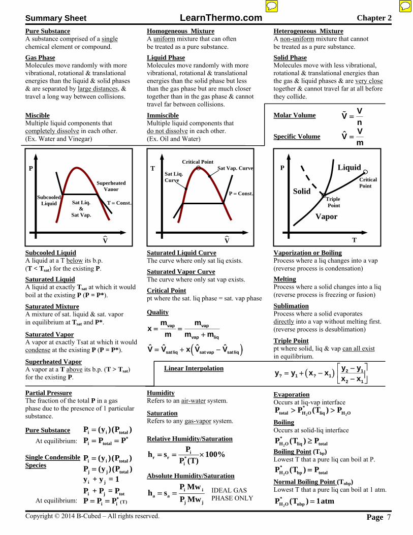
Pure Substance A substance comprised of a single chemical element or compound. Gas Phase Molecules move randomly with more vibrational, rotational & translational energies than the liquid & solid phases & are separated by large distances, & travel a long way between collisions.
Miscible Multiple liquid components that completely dissolve in each other.(Ex. Water and Vinegar)
Homogeneous Mixture A uniform mixture that can often be treated as a pure substance. Liquid Phase Molecules move randomly with more vibrational, rotational & translational energies than the solid phase but less than the gas phase but are much closer together than in the gas phase & cannot travel far between collisions.
Immiscible Multiple liquid components that do not dissolve in each other. (Ex. Oil and Water)
Heterogeneous Mixture A non-uniform mixture that cannot be treated as a pure substance. Solid Phase Molecules move with less vibrational, rotational & translational energies than the gas & liquid phases & are very close together & cannot travel far at all before they collide.
Molar Volume
Specific Volume
V
P
T Const.Sat Liq. &
Sat Vap.
Superheated Vapor
Subcooled Liquid
V
TCritical Point
P Const.
Sat Liq. Curve
Sat Vap. Curve
Vapor
Liquid
Solid
P
T
Critical Point
Triple Point
Subcooled Liquid A liquid at a T below its b.p. (T < Tsat) for the existing P. Saturated Liquid A liquid at exactly Tsat at which it would boil at the existing P (P = P*).
Saturated Mixture A mixture of sat. liquid & sat. vapor in equilibrium at Tsat and P*.
Saturated Vapor A vapor at exactly Tsat at which it would condense at the existing P (P = P*).
Superheated Vapor A vapor at a T above its b.p. (T > Tsat) for the existing P.
Saturated Liquid Curve The curve where only sat liq exists. Saturated Vapor Curve The curve where only sat vap exists. Critical Point pt where the sat. liq phase = sat. vap phase
Quality
Linear Interpolation
Melting Process where a solid changes into a liq (reverse process is freezing or fusion)
Vaporization or Boiling Process where a liq changes into a vap (reverse process is condensation)
Sublimation Process where a solid evaporates directly into a vap without melting first. (reverse process is desublimation)
Triple Point pt where solid, liq & vap can all existin equilibrium.
i i totalP (y )(P )
Partial Pressure The fraction of the total P in a gas phase due to the presence of 1 particular substance.
j j totalP (y )(P )i jy + y = 1
i j totP + P = P
i totalP P P
(T)i iP P P
Pure Substance
At equilibrium:
Single Condensible Species
i i totalP (y )(P )
At equilibrium:
i ia a
j j
P Mwh s
P Mw
ir r *
i
Ph s 100%
P (T)
Humidity Refers to an air-water system.
Saturation Refers to any gas-vapor system.
Relative Humidity/Saturation
Absolute Humidity/Saturation
IDEAL GAS PHASE ONLY
Evaporation Occurs at liq-vap interface
2 2
*total H O liq H OP P (T ) P
Boiling Occurs at solid-liq interface
2
*H O liq totalP (T ) P
Boiling Point (Tbp) Lowest T that a pure liq can boil at P.
2
*H O bp totalP (T ) P
Normal Boiling Point (Tnbp) Lowest T that a pure liq can boil at 1 atm.
2
*H O nbpP (T ) 1atm
Chapter 2
VV
n
VV
m
2 1? 1 ? 1
2 1
y yy y x x
x x
vap vap
vap liq
m mx
m m m
sat liq sat vap sat liqˆ ˆ ˆ ˆV V x V V

Summary Sheet LearnThermo.com
Page 8Copyright © 2014 B-Cubed - All Rights Reserved.
Equations of State (EOS) An equation that relates P, T & molar V of a substance.
PV nRTPV RT
Ideal Gas EOS Good approximation at high T (above 0oC) & low P (1 atm or less).
Universal Gas Constant
Critical Properties Properties at the critical point such as the critical T, critical P & critical molar V (although the ideal critical molar volume is ofen used instead).
idealC C CV RT / PPV
ZnRT
PV nZRTPV ZRT
Graphical EOS: Compressibility Charts Z accounts for the deviation from IG.
2 2 2
C2
C
27 R T P Va
64 P mol
2
RT aP
V b V
C
C
R Tb 0.08664
P
2 5 / 2C
C
R Ta 0.42748
P
1/ 2
RT aP
V b V V b T
Redlich-Kwong Modification of the Van der Waal EOS which includes a correction for the T dependence of the Van der Waal attraction term.
Virial EOS Based on the IG EOS where Z is expanded as an infinite power series.
2
PV B(T) C(T)Z 1 ...
RT V V
PV B(T)Z 1
RT V
Truncated Virial EOS
ideal true
true
X X100
X
Ideal Gas at Std. Cond.
V RT P 20L/ mol
1% if :
Ideal Gas EOS Validity
V RT P 5L/ mol
for most gases
for diatomic & noble gases
Reduced Properties Dimensionless properties determined from critical properties.
Species Ammonia 0.250 Argon - 0.004 Carbon Dioxide 0.225 Carbon Monoxide 0.049 Chlorine 0.073 Ethane 0. 098 Hydrogen Sulfide 0.100 Methane 0.008 Methanol 0.559 Nitrogen 0.040 Oxygen 0. 021 Propane 0. 152 Sulfur Dioxide 0.251 Water 0. 344
Van der Waal EOS Constant b accounts for the volume the molecules occupy. a/V2 accounts for attractive forces between molecules (Van der Waal’s forces).
~
o0 C, 1atm: 22.415L / mol
C
C
RT Vb
8P mol
RC
TT
TR
C
PP
P
idealR ideal
C CC
V VV
RT / PV
2
R1 m 1 T
2m 0.48508 1.55171 0.1561
C
C
R Tb 0.08664
P
2 2C
C
R Ta 0.42748
P
R T a
PV b V V b
Soave-Redlich-Kwong
C0 1
C
RTB B B
P
0 1.6R
0.422B 0.083
T
1 4.2R
0.172B 0.139
T
Estimating the first virial coefficient:
Chapter 2
3
3
f
3
8.3144621 kJ/kmol K
8.3144621 kPa m /kmol K
0.083144621 bar m /kmol K
82.05746 L atm/kmol K
1.985884 Btu/lbmol R
1545.348 ft lb /lbmol R
10.73159 psia ft / lbmol R
R =


22
Introduction: Basic Concepts
of Thermodynamics
In this chapter, you will discover the nature of thermodynamics and how it effects your life. The scope of this book is provided so you will know what you will and will not learn. Many of the key terms that are used to discuss thermodynamics are introduced and explained.
Used by permission from Trane
Ch
ap
ter
1
Ch
ap
ter
1

Workbook LearnThermo.com Chapter 1
Basic Concepts of Thermodynamics Page 23
Thermo touches the lives of most people asa means of transportation.
Heating and cooling systems make manypeople’s lives more comfortable and keep food from spoiling.
Thermo is also the key to electrical powergeneration.
If you live in a mild climate, such as Seat-tle’s, you may have one of these behind your house.
Ever wonder what is inside or how itworks ?
How Does Thermo Affect You ?
Engines: Trains, Planes & Automobiles Heating Systems: Heat Pumps Cooling Systems:
Air Conditioning Refrigeration
Others: Aspects of Thermo that are beyond the scope of this
course make it a key aspect of chemical and biologi-cal systems
Water-Source Heat Pump
Used by permission from Trane

Workbook LearnThermo.com Chapter 1
Page 24 Basic Concepts of Thermodynamics
Looks kind of complicated. Reversible heat pumps, like this one, can
also be used as air-conditioners So, what is the purpose of this device ?
In cooling mode, the heat pump uses elec-trical work to transfer heat from cool air (inside your home) into the warm air (outside your home).
The cool part is that, for each Watt ofelectrical power used by the A/C unit, more than one Watt of energy is removed from the air inside your home.
Not bad ! What happens when the reversing valve is
switched ?
Water-Source Heat Pump
refrigerant-to-water heat exchanger
refrigerant-to-air heat exchanger
compressor
reversing valve
expansion device
compressor
reversing valve
refrigerant-to-water heat exchanger
water loop
Used by permission from Trane
Heat Pump in Cooling Mode
expansion device
refrigerant-to-air heat exchanger

Workbook LearnThermo.com Chapter 1
Basic Concepts of Thermodynamics Page 25
In heating mode, the heat pump uses electri-cal work to transfer heat from cool air (outside your home) into the warm air (inside your home).
The cool part is that, for each Watt of elec-trical power used by the heat pump unit, more than one Watt of energy is added to the air inside your home.
So, a heat pump is more efficient than anelectrical resistance heater ! Nice.
A refrigerator works in much the same waythat a heat pump does.
In fact an A/C unit is technically a refrigera-tor because the purpose is to keep the cool space cool.
The Continuum Scale A large group of molecules is larger than
100 mm across Behavior of individual molecules is not
studied Only the properties of the large group of
molecules are studied: think P, V and T 1st Law – Energy is a conserved quantity
This is the basis for much of this course. 2nd Law – A simple and sensible idea,
right ? The implications of the 2nd law are
ENORMOUS Forms of Energy
There are many types of potential energy,but we will generally only consider gravita-tional potential energy
I suspect you already have a pretty goodunderstanding of Kinetic Energy
You were introduced to Internal Energy ingeneral chemistry, but in this class, you will learn a lot more about how to use this quan-tity to solve problems.
Classical Thermodynamics
Heat Pump in Heating Mode
compressor
reversing valve
refrigerant-to-water heat exchanger
water loop
Used by permission from Trane
expansion device
refrigerant-to-air heat exchanger
Large Groups of Molecules – Continuum Scale The Laws of Thermodynamics
1st Law: Energy can neither be created nor destroyed. It can onlychange form.
2nd Law: Energy in the form of heat only flows spontaneously fromregions of higher temperature to regions of lower temperature.
Forms of Energy
Gravitational Potential
Kinetic
Internal Heat Work
PC
gE m z
g P
C
gE z
g
2
KC
1 vE m
2 g
2
KC
1 vE
2 g
UQ
W W
Q
U

Workbook LearnThermo.com Chapter 1
Page 26 Basic Concepts of Thermodynamics
Dimensions are more fundamental thanunits
Other dimensions include electrical chargeand temperature
Units are not very difficult except when wemust convert between systems of units, such as AE and SI.
The easiest way to keep this straight is touse gc and Newton’s 2nd Law of Motion.
We will work a problem using this in class. Online, I like the FootRule website. Check
it out !
Systems The entire universe is divided into two re-
gions: the system and the surroundings. The surface that separates the system from
the surroundings is called the boundary of the system.
If mass flows across the system boundary,then the system is called OPEN.
If NO mass flows across the system bound-ary, then the system is called CLOSED.
Properties Intensive properties are more important in
this course because they determine the STATE of the system.
Molar and specific properties are intensivevariables. We will use them MUCH more than we will use extensive properties, such as volume.
States Consider a system that contains a pure sub-
stance in a single phase. If we measure just TWO intensive properties
of the system, then we don’t need to measure any more properties.
They are all fixed and could be determinedfrom the two values that we measured.
This cool part is a special case of the GibbsPhase Rule. We’ll learn more about this in Lesson 3C.
Terminology or Nomenclature
Dimensions & Units
Dimensions: Mass, Length, Time Units: m, ft, kg, lbm, J, Btu Force
IS a fundamental unit in the AE System Is NOT a fundamental unit in the SI System Newton’s 2nd Law of Motion:
AE:
SI:
Conversion Factors Download from the course website Online: “The Foot Rule” website
http://www.FootRule.com
mC 2
f
lb ftg 32.174
lb s
C 2
kg mg 1
N s
Cg F ma
System: The material or volume that we are studying Systems have boundaries Closed Systems: Mass does not cross the boundary Open Systems: Mass does cross the boundary
Properties Intensive vs. Extensive Properties
Extensive properties depend on the size of the system, in-tensive properties do not.
Molar Properties: per mole. Molar volume:
Specific Properties: per kg or per lbm. Specific volume: States
The condition of a piece of matter or system as determined by itsintensive properties.
If ANY intensive property is different, then the system is in adifferent state.
V
V

Workbook LearnThermo.com Chapter 1
Basic Concepts of Thermodynamics Page 27
Most of the problems we solve in thiscourse will involve the analysis of processes
One key to understanding the effects of anyprocess on a system is to know which states the system passes through during the proc-ess. That is, we need to understand the process path
Special types of processes are a little biteasier to analyze because one property does not change.
These are the big three special processes,but we will add 3 or 4 more special types of processes later in the course.
Cycles are special and cool types of proc-esses.
Engines, refrigerators and heat pumps alloperate on Thermodynamic Cycles.
Analysis of cycles is the ultimate goal ofthis course !
Equilibrium For a system to truly be in equilibrium, it
must be in equilibrium thermally, chemi-cally, mechanically and it must be in phase equilibrium as well.
Quasi-Equilibrium Processes All forces are balanced or nearly balanced
throughout the process Q-E processes must occur very slowly so
the system only deviates slightly from equilibrium.
Although no real process is actually a Q-E process, we can use the Q-E process as a best case.
Then we can compare the performance of real processes to the performance of equivalent Q-E processes.
Equilibrium
More Nomenclature
Process A change in the state of a system
Process Path The series of states that a system moves through on its way from the
initial state to the final state. Special Types of Processes
Isobaric – constant pressure Isothermal - constant temperature Isochoric - constant volume
Cycles Special process paths in which the initial state is the same as the
final state Thermodynamic cycles are a key topic in this course
A system is in equilibrium when no unbalanced potentialsor driving forces exist within the system boundary.
Thermal: no temperature driving forces Chemical: no chemical driving forces Phase: no mass transfer driving forces Mechanical: no unbalanced mechanical forces
Quasi-Equilibrium Processes A process during which the system only deviates from equi-
librium by an infinitessimal amount. Every state along the process path is very nearly an equilib-
rium state.

Workbook LearnThermo.com Chapter 1
Page 28 Basic Concepts of Thermodynamics
Volume is pretty straightforward and theunits should be very familiar.
The units of pressure for SI may not all befamiliar.
My favorite unit for pressure is the kPa. 1atm = 101.325 kPa = 14.696 psia
Oddly enough, there are different types ofpressures.
Before today, you only worked with abso-lute pressure and that is what you want to continue to use.
So, if you are given a vacuum pressure orgage pressure, the first thing you want to do is convert it to absolute pressure.
Pgage = Pabs – Patm
Pvac = Patm – Pabs
Remember that absolute pressure cannot benegative, but gage pressure can.
Technically, vacuum pressure can be nega-tive, but it is not usually expressed as vac-uum pressure in that case.
The barometer eqn helps you calculate thepressure the bottom of a tank, P2, given the pressure at the top of the tank, P1, and the depth and density of the fluid.
Remember that the pressure at the bottomof the tank is always greater than the pres-sure at the surface of the liquid.
A manometer lets you calculate the differ-ence between the pressure in two different locations, such as the difference between the pressure inside a tank and the ambient pressure.
All you need to know is the density of themanometer fluid and the difference in the height of the manometer fluid in the two legs of the manometer. (assuming the den-sity of the fluid in the tank is negligible, usually this means it is a gas).
The differential manometer eqn lets youcalculate the difference in pressure between two locations, even if the fluid density is similar to the density of the manometer fluid.
This is especially useful for measuring thepressure drop that occurs as a fluid flows through a pipe.
Manometers
Pressure, Volume & Temperature
Volume:
SI: L, m3, mL=cm3
AE: ft3
Pressure: acts in all directions to all surfaces SI: Pa, kPa, MPa, bar, atm AE: psia Absolute, Gage and Vacuum Pressures
VV
n V
Vm
m 1
ˆV V
Barometer Eqn:
Manometer Eqn:
DifferentialManometer Eqn:
2 1 fc
gP P h
g
in out fc
gP P h
g
up down m fc
gP P h
g

Workbook LearnThermo.com Chapter 1
Basic Concepts of Thermodynamics Page 29
Engineers usually use thermocouples orother temperature measuring devices be-cause they are well-suited to electronic data acquisition.
Ideal Gas Thermometers provide some ofthe most accurate temperature measure-ments available.
The downside is that several experimentsmust be run at decreasing pressure so the results can be extrapolated back to ZERO pressure.
Why ? Because only at zero pressure is anyreal gas actually ideal.
Once this calibration is complete, the IGThermometer is ready to measure the tem-perature of a sample of the same gas that was used in the calibration.
In order to measure the temperature of adifferent gas, the IG Thermometer must be recalibrated.
The IG thermometer is very accurate, butnot practical for most applications.
Temperature
Thermometers and Thermocouples Temperature conversions are straightforward T (oC) = T(K) and T (oF) = T(oR) Ideal Gas Thermometry
Must be calibrated Tedious, but extremely accurate IG T-scale is identical to the Kelvin Scale !

1A-1 6 pts
Read :
Given: g(m/s2) = a - b * h v 750 km/ha 9.8066 m/s2 h 12000 mb 3.20E-06 s-2 Wsea level 50 kN
gc 1 kg-m/N-s2
Find: a.) Ekin ??? MJ b.) Epot ??? MJ
Assumptions:
Equations / Data / Solve :
Newton's 2nd Law of Motion: Eqn 1
or Eqn 2
g 9.8066 m/s2
Eqn 3
m 5099 kgNow, we are ready to solve the rest of the problem.
Part a.) The definition of kinetic energy is : Eqn 4
Ek 1.106E+08 JEk 111 MJ
At sea level, according to the eqn given in the problem statement, the acceleration of gravity is :
Now, we can solve Eqn 1 for m and plug in values :
Since gravitational acceleration is LESS at higher altitude, the gravitational potential energy of the airplane will not be quite as great as you might ordinarily expect. We need the weight of the airplane at sea level in order to determine the mass of the airplane. We need ot know the mass in order to calculate both the kinetic and gravitation potential energies of the plane.
1- Gravitational acceleration is a function of altitude only.
Let's begin by determining the mass of the airplane from the weight at sea level.
Gravitational acceleration is less at higher altitudes than at sea level. Assume gravitational acceleration as a function of
altitude is described by g(m/s2) = 9.806 - 3.2 x 10⁻⁶ * h, where h is the altitude (relative to sea level).
Consider an aircraft flying at 750 km/h at an altitude of 12 km. Before take-off, the aircraft weighed 50 kN at sea level. Determine its:a.) kinetic energyb.) potential energy relative to sea level.
Kinetic and Potential Energy of an Airplane in Flight
g F mac
c sea levelg W m g
csea level
gm W
g
2
KC
1 vE m
2 g
Dr. B - LearnThermo.com Ex 1A-1 Copyright B-Cubed 2014, all rights reserved

Part b.)
Eqn 5
Let's think about this part a bit more carefully. Eqn 6
Eqn 7
Eqn 8
Eqn 9
Epot 5.988E+08 J Epot 598.8 MJ
or : Eqn 10
Answers : a.) Ek 111 MJ b.) Epot 599 MJ
So, the average effective value of the gravitational acceleration for determining the potential energy of the airplane in this problem is equal to the gravitational acceleration at HALF of the actual altitude of the airplane.
Would this be true if g = a - b x -c x2 ?? Nope. What is special about the equation for g given in this problem that leads to the interesting result in Eqn 10 ?
Now, if m, g and gc are all constants, Eqn 7 simply reduces to Eqn 5 because the integral of dx from 0 to h is
just h. In our problem, however, g is NOT a constant. Therefore :
So, what "average" value of g should we have used in Eqn 5 ? Let's combine Eqns 5 and 8 and see what we get.
The differential increase in the potential energy of an object infinitessimally above sea level is:
So, the gravitational potential energy of anoject that is a distance h above sea level is :
The definition of gravitational potential energy, relative to sea level, is :
The problem is what value of g do we use ? Do we simply use g at the altitude of the plane? Or do we use some sort of average value of g ?
PC
gdE m dx
g
PE h
P P0 0 C
gE dE m dx
g
hg a b
2 C C
g m hm h a b h
g g 2
h2 2h
P0C C C C0
m m x m h m hE a bx dx ax b ah b a b h
g g 2 g 2 g 2
PC
gE m h
g
PC
gE m h
g
Dr. B - LearnThermo.com Ex 1A-1 Copyright B-Cubed 2014, all rights reserved

1A-2 5 pts
Read:
Given: Eqn 1 K = spring constant
x = displacement of the spring, in this case compression.
m 50000 kgv 2.4 m/s gc 1 kg-m/N-s2
x 0.6 m
Find: K ??? N/m
Assumptions: 1- The spring is a linear spring and therefore the given equation applies.2- All of the kinetic energy of the boat is absorbed by the springs.
Equations / Data / Solve:
Eqn 2
Because there are two identical springs : Eqn 3
Plugging given values into Eqn 2 and Eqn 3 yields: Ekin 144000 JEspring 72000 J
Next, we can solve Eqn 1 algebraically for the spring constant, K. Eqn 4
It is important to note that two springs are used to stop the vehicle.All of the initial kinetic energy of the vehicle must be absorbed by the springs and converted to spring potential energy.
The key to solving this problem is to recognize that the final potential energy of the two springs must be equal to the initial kinetic energy of the vehicle. So, we should begin by calculating the initial kinetic energy of the boat.
Conversion of Kinetic Energy into Spring Potential Energy
It takes energy to compress a spring. This energy is stored as spring potential energy, which can be calculated using: Espring
= 1/2 K x2, where K is the spring constant and x is the distance the spring is compressed.At a dock, a boat with a mass of 50,000 kg hits a bumper supported by two springs that stop the boat and absorb its kinetic energy.
Determine the spring constant of the springs that is required if the maximum compression is to be 60 cm for a boat speed of 2.4 m/s.
2spring
1E K x
2=
2kin
c
1E mv
2g=
kinspring
EE
2=
spring
2
2 EK
x=
Dr. B - LearnThermo.com Ex 1A-2 Copyright B-Cubed 2014, all rights reserved

First, let's work on the units. Eqn 5
Now, let's calculate the value of the spring constant. K 4.00E+05 N/m
Answers: K 4.00E+05 N/m
[ ] [ ] [ ]2 2
J N m NK
mm m
⋅= = =
Dr. B - LearnThermo.com Ex 1A-2 Copyright B-Cubed 2014, all rights reserved
1B-1 4 pts
Read:
Given: m 124 lbm a 5.3 ft/s2
Find: a.) Fwt ??? lbf b.) mbeam ??? lbm
Assumptions:
Equations / Data / Solve:
Part a.)Eqn 1
Eqn 2
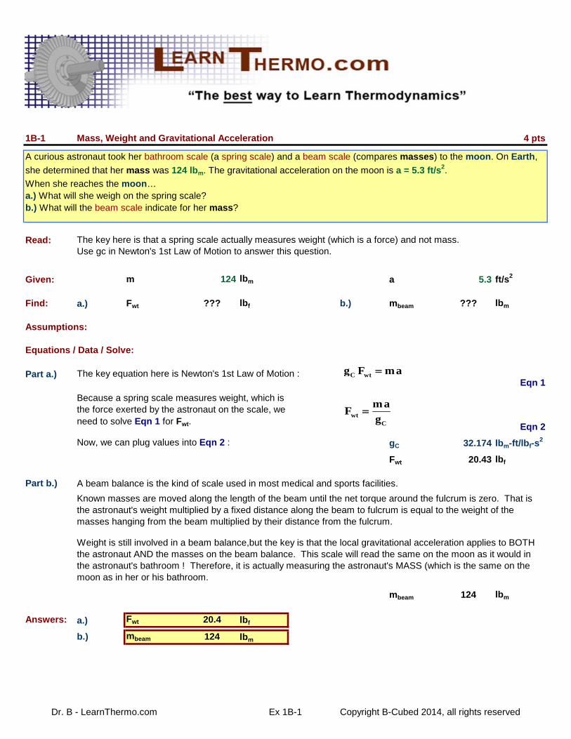
Now, we can plug values into Eqn 2 : gC 32.174 lbm-ft/lbf-s2
Fwt 20.43 lbf
Part b.)
mbeam 124 lbm
Answers: a.) Fwt 20.4 lbf
b.) mbeam 124 lbm
Because a spring scale measures weight, which is the force exerted by the astronaut on the scale, we need to solve Eqn 1 for Fwt.
A beam balance is the kind of scale used in most medical and sports facilities.
Known masses are moved along the length of the beam until the net torque around the fulcrum is zero. That is the astronaut's weight multiplied by a fixed distance along the beam to fulcrum is equal to the weight of the masses hanging from the beam multiplied by their distance from the fulcrum.
Weight is still involved in a beam balance,but the key is that the local gravitational acceleration applies to BOTH the astronaut AND the masses on the beam balance. This scale will read the same on the moon as it would in the astronaut's bathroom ! Therefore, it is actually measuring the astronaut's MASS (which is the same on the moon as in her or his bathroom.
When she reaches the moon…a.) What will she weigh on the spring scale?b.) What will the beam scale indicate for her mass?
Mass, Weight and Gravitational Acceleration
A curious astronaut took her bathroom scale (a spring scale) and a beam scale (compares masses) to the moon. On Earth,
she determined that her mass was 124 lbm. The gravitational acceleration on the moon is a = 5.3 ft/s2.
The key here is that a spring scale actually measures weight (which is a force) and not mass.Use gc in Newton's 1st Law of Motion to answer this question.
The key equation here is Newton's 1st Law of Motion : C wtg F ma
wtC
maF
g
Dr. B - LearnThermo.com Ex 1B-1 Copyright B-Cubed 2014, all rights reserved

1B-2 4 pts
Read:
Given: m 2 kg g 9.74 m/s2
Fthrow 100 N
Find: a ??? m/s2
Assumptions: None.
Equations / Data / Solve:
Eqn 1
Eqn 2
We know that : gC 1 kg-m/N-s2
Eqn 3
Eqn 4
We can solve Eqn 4 for Fwt, as follows : Eqn 5
Fwt 19.5 NFnet 80.52 N
a 40.26 m/s2
Answers: a 40.3 m/s2
The net force acting on the rock in the upward direction is :
We can apply Newton's 1st Law of Motion again to evaluate Fwt.
Plugging values into Eqn 5, then Eqn 3 and, finally, Eqn 2 yields :
The key here is to recognize that two forces are acting on the rock: the 100 N and the weight of the rock (due to gravity). Then, the problem becomes an application of Newton's 1st Law of Motion.
The key equation here is Newton's 1st Law of Motion :
We can solve Eqn 1 for the rate at which the rock accelerates :
So, all we need to is determine the net force acting on the stone.
A free-body diagram might be helpful.
Mass, Force and Acceleration
A strong boy throws a rock straight up with a force of 100 N. At what rate does the rock initially accelerate upwards, in m/s2?
Assume the mass of the rock is 2 kg and the local gravitational acceleration is 9.74 m/s2.
C netg F ma
C netg Fa
m
Rock
Fwt
Fthrow
net throw wtF F F
C wtg F mg
wtC
gF m
g
Dr. B - LearnThermo.com Ex 1B-2 Copyright B-Cubed 2014, all rights reserved

1B-3 4 pts
Read:
Given: mCO2 0.5 kg CO2 / kW-h Power 350 kW-h/house/yearN 500000 houses
Find: MCO2 ??? mton CO2 / year
Assumptions: None.
Equations / Data / Solve:
Eqn 1
Check the units in this equation :
Eqn 2
Plug in the values : MCO2 8.75E+07 kg CO2 / year
Unit conversion factor : 1 metric ton = 1000 kg
Therefore : MCO2 87500 mton CO2 / year
Answers: MCO2 87500 mton CO2 / year
Units and Carbon Dioxide Emissions
A new, energy-efficient home refrigerator consumes about 350 kW-h of electricity per year. Assume the electricity is generated by burning fossil fuels. When fossil fuels like coal, oil, natural gas and gasoline are burned, most of
the carbon in the fuel burns completely to form carbon dioxide (CO2). CO2 is a greenhouse gas that contributes to global
warming and that is undesirable. In a typical natural gas power plant, 0.5 kg of CO2 is produced for each
kW-h of electricity generated. Consider a city with 500,000 homes with one refrigerator in each home. How much CO2, in
metric tons, is produced by the refrigerators in the city in one year?
This problem is all about unit conversions.Keep careful track of units and it will not be difficult.A kW-h is unit of energy. A Watt is energy per time and when you multiply by hours (time) you are left with units of energy. A kW-h is kW times hours. It is the amount of energy consumed in an hour by a device that uses 1 kW of power (1 kJ/s for 3600 sec).
The total mass of CO2 produced per year is the product of the rate of CO2 production per kW-h, the rate at which power is used by each house and the number of houses.
CO2 CO2 housesM Power m N
2 2CO2
kgCO kgCOkW hM house
house year kW h year
Dr. B - LearnThermo.com Ex 1B-3 Copyright B-Cubed 2014, all rights reserved

1B-4 4 pts
Read:
Given: m 35000 lbm gc 32.174 lbm-ft/lbf-s2
a 125 ft/s2
Find: Fup ??? lbf
Assumptions: 1- Assume: g 32.174 ft/s2
Equations / Data / Solve:
We begin with Newton's 2nd Law of Motion : Eqn 1
Eqn 2
We can now substitute Eqn 1 into Eqn 2 to get :
Eqn 3
Now, we can plug in the values : atotal 157.174 ft/s2
Fwt 35000 lbf
Facc 135979 lbf
Ftotal 170979 lbf
Answers: Fup 171000 lbf
Force Required to Accelerate a Rocket
NASA would like a rocket to accelerate upward at a rate of 125 ft/s2. The mass of the rocket is 35,000 lbm. Determine the
upward thrust force, in lbf, that the rocket engine must produce.
This is a direct application of Newton's 2nd Law of Motion in the AE System of units.The key to solving this problem is a clear understanding of gc.
The force required to lift the rocket and accelerate it upward depends on both the weight of the rocket (and
therefore the g) and the rate at which the rocket must be accelerated…120 ft/s2. Therefore:
Note, in the absence of gravity, weightlessness, it would still require a force of Facc = 135,979 lbf to accelerate
the rocket at a rate of 125 ft/s2.
cg F ma
up weight accelerateF F F
totalup
c c c c
g a am g maF m m
g g g g
Dr. B - LearnThermo.com Ex 1B-4 Copyright B-Cubed 2014, all rights reserved

1B-5 5 pts
Read:
Given: Patm 100 kPa H2O 1000 kg/m3
gc 1 kg-m/N-s2 Hg 13600 kg/m3
a.) Pgage 17 kPa c.) Pabs 55 mmHgb.) Pabs 225 kPa d.) Pgage 32 m H2O
Assumptions: 1- Assume: g 9.8066 m/s2
Find: Pgauge ??? kPa Pabs ??? mmHgPabs ??? kPa Pgauge ??? m H2O
Equations / Data / Solve:
There are two key relationships in the solution to this problem.The first is the relationship between absolute and gage pressure :
Eqn 1
Eqn 2
Now, let's see how we use these 2 equations to complete the table.
Part a.)
The reason we use the Manometer Equation is that when a pressure unit involves a length of a given fluid, as in the last two columns of the table given in this problem, it really means that this is the height that an open-ended manometer (for gage pressure) or a closed end manometer (for absolute pressure) would read if the given fluid were used as the manometer fluid.
Eqn 3In order to fill in the 2nd column, we must solve Eqn 1 for the absolute pressure :
This problem requires an understanding of the relationship between absolute and gage pressure.It will also require the effective use of unit conversions.
The second relationship is required in order to make sense of the units for pressure in the last two columns of the table in the problem statement. The 2nd relationship is the Manometer Equation.
Relationships between Different Types of Pressures
Fill in the blank values in the table below. Assume Patm = 100 kPa and the density of liquid mercury (Hg) is 13,600 kg/m3.
gage abs atmP P P
abs gage atmP P P
in out fc
gP P h
g
Dr. B - LearnThermo.com Ex 1B-5 Copyright B-Cubed 2014, all rights reserved

Therefore : Pabs 117 kPa
Eqn 4
Eqn 5
Be sure to convert kPa to Pa=N/m2 when plugging values into Eqn 5.
Pabs = h = 0.877 m Hg Pabs 877 mm Hg
In this case, Pin = Pabs and Pout = Patm (because it is a closed-end manometer).
Eqn 6
Eqn 7
Pgage = h = 1.7335 m H2O Pgage 1.734 m H2O
Parts b-d)
Answers: Pgage
(kPa)
Pabs
(kPa)
Pabs
(mmHg)
Pgage
(m H2O)
a.) 17 117 877 1.73b.) 125 225 1690 22.9c.) -92.7 7.34 55 -0.909d.) 314 414 3100 32
The solution of the remaining parts of this problem involve the algebraic manipulation of Eqns 1, 3, 5 and 7, but does not involve any additional concepts, techniques or data. The final answers to parts b through d are provided in the table below.
Column 4 requires a gage pressure, so the open-end form of the Manometer Equation is used :
Next, we solve Eqn 6 for h and make use of Eqn 1 if we want to use the given value of the gage pressure.
In this case, Pin = Pabs and Pout = 0 (because it is a closed-end manometer).
Actually, Pout should be equal to the vapor pressure of the manometer fluid, but that is a topic for chapter 2.
Therefore, Eqn 2 becomes :
In this case, the answer for column 3 is actually the value of h, so we need to solve Eqn 4 for h :
To complete column 3, we must convert the units from our result for Pabs using Eqn 2.
This is somewhat arbitrary since the problem statement does not make it very clear how many significant figures exist in the given information. When in doubt, 3 significant figures is a reasonable choice.
Notice that I chose to use 3 significant figures in my answers.
abs c
Hg
P gh
g
abs Hgc
gP h
g
abs atm H2Oc
gP P h
g
gageabs atm c c
H2O H2O
PP P g gh
g g
Dr. B - LearnThermo.com Ex 1B-5 Copyright B-Cubed 2014, all rights reserved
1B-6 5 pts
Read:
Given: D 0.2 m gc 1 kg-m/N-s2
h 3 m
Find: Fup ??? kN
Assumptions: 1- Assume: g 9.8066 m/s2
Patm 100 kPaH2O 1000 kg/m3
Equations / Data / Solve:
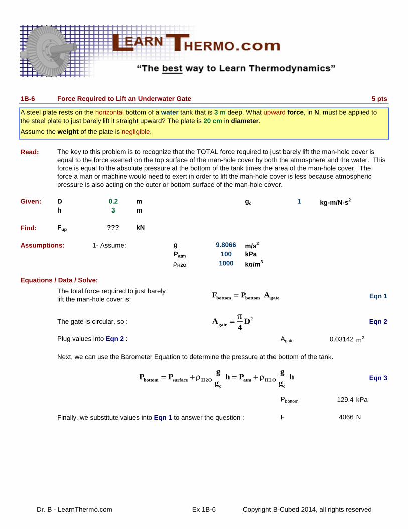
The gate is circular, so : Eqn 2
Agate 0.03142 m2
Eqn 3
Pbottom 129.4 kPa
F 4066 N
Next, we can use the Barometer Equation to determine the pressure at the bottom of the tank.
Plug values into Eqn 2 :
Finally, we substitute values into Eqn 1 to answer the question :
Assume the weight of the plate is negligible.
Force Required to Lift an Underwater Gate
A steel plate rests on the horizontal bottom of a water tank that is 3 m deep. What upward force, in N, must be applied to the steel plate to just barely lift it straight upward? The plate is 20 cm in diameter.
The key to this problem is to recognize that the TOTAL force required to just barely lift the man-hole cover is equal to the force exerted on the top surface of the man-hole cover by both the atmosphere and the water. This force is equal to the absolute pressure at the bottom of the tank times the area of the man-hole cover. The force a man or machine would need to exert in order to lift the man-hole cover is less because atmospheric pressure is also acting on the outer or bottom surface of the man-hole cover.
The total force required to just barely lift the man-hole cover is: Eqn 1
bottom surface H2O atm H2Oc c
g gP P h P h
g g
bottom bottom gateF P A
2gateA D
4
Dr. B - LearnThermo.com Ex 1B-6 Copyright B-Cubed 2014, all rights reserved
Eqn 4
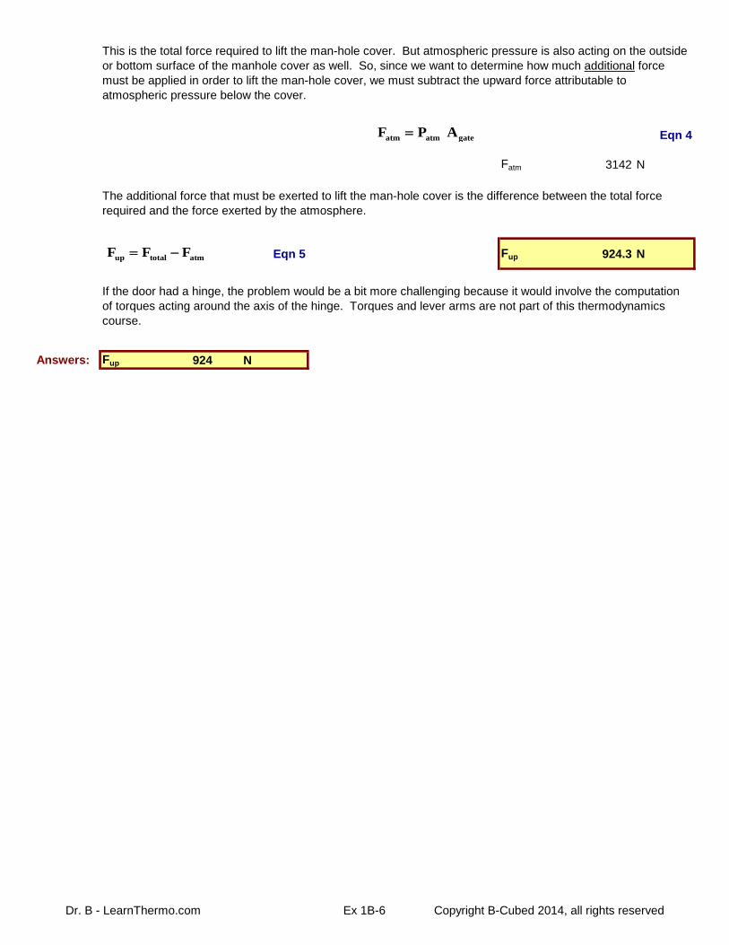
Fatm 3142 N
Eqn 5 Fup 924.3 N
Answers: Fup 924 N
This is the total force required to lift the man-hole cover. But atmospheric pressure is also acting on the outside or bottom surface of the manhole cover as well. So, since we want to determine how much additional force must be applied in order to lift the man-hole cover, we must subtract the upward force attributable to atmospheric pressure below the cover.
The additional force that must be exerted to lift the man-hole cover is the difference between the total force required and the force exerted by the atmosphere.
If the door had a hinge, the problem would be a bit more challenging because it would involve the computation of torques acting around the axis of the hinge. Torques and lever arms are not part of this thermodynamics course.
atm atm gateF P A
up total atmF F F
Dr. B - LearnThermo.com Ex 1B-6 Copyright B-Cubed 2014, all rights reserved

1B-7 5 pts
Read: 1 Zerf exerts 1 Spund of force when a = 3.7 m/s2.
Given: amoon 3.7 m/s2
m 350 Zerf
Find: a.) gc ??? m-Zerf/Spund-s2
b.) Fwt ??? Spund for mMars 350 Zerfc.) Fwt ??? Spund for mEarth 350 Zerfd.) Is this Z-S system similer to the SI or AE system?
Assumptions: 1- The acceleration of gravity at the surfae of the Earth is: aEarth 9.8066 m/s2
Equations / Data / Solve:
Eqn 1
Part a.) Eqn 2
gc 3.70 m-Zerf/Spund-s2
Solve Newton's 2nd Law for gc :
Newton's 2nd Law :
d.) To which system of units is the Zerf-Spund system most similar, SI or AE?
The key here is that Newton's 2nd Law of Motion applies regardless of where the system is located or what system of units is used.
Mass, Weight and Gravitational Acceleration: Keebos and Tweeks
In the future, we may encounter a civilization from another planet. They will not use the SI or AE systems of units. Suppose we meet aliens who use the Zerf as a unit of mass and the Spund as a unit of force.
One Spund is the weight of a mass of one Zerf on the surface of Mars. The gravitational acceleration on Mars is 3.7
m/s2.a.) What is gc in the alien system of units? Be sure to include the numerical value and the units.
b.) How much would a 350 Zerf object weigh on the surface of Mars, in Spunds?c.) How much would a 350 Zerf object weigh on the surface of the Earth, in Spunds?
cg F ma=
c
mag
F=
( )( )2
c
1 Zerf 3.7m / sg
1 Spund=
Dr. B - LearnThermo.com Ex 1B-7 Copyright B-Cubed 2014, all rights reserved

Part b.) Eqn 3
Fwt 350 Spund
Part c.) Eqn 4
Fwt 928 Spund
There are two important points to this problem:1 - The value of gc is the same everywhere in the universe.
Part d.)
Answers: a.) gc 3.70 m-Zerf/Spund-s2
b.) Fwt 350 Spund
c.) Fwt 930 Spund
d.) AE
Solve Newton's 2nd Law for F :
Solve Newton's 2nd Law for F :
2 - If a person weighs a certain amount more on the Earth than on Mars in one system of units, then he or she also weighs proportionally more on the Earth than on Mars in any other sytem of units as well !
The Zerf-Spund system of units is analogous to the American Engineering System of units because gc is not equal to 1 and 1 unit of mass exerts 1 unit of force (on the Mars).
c
maF
g=
( )( )2
2
350 Zerf 3.7m / sF
3.7 m Zerf / Spund s=
⋅ ⋅
c
maF
g=
( )( )2
2
350 Zerf 9.8066m / sF
3.7 m Zerf / Spund s=
⋅ ⋅
Dr. B - LearnThermo.com Ex 1B-7 Copyright B-Cubed 2014, all rights reserved


1E-1 6 pts
Read:
Given: h1 0.24 m w 1000 kg/m3
h2 0.35 m oil 790 kg/m3
h3 0.52 m Hg 13600 kg/m3
P2 101.325 kPa
Find: P1,gauge ??? kPa gauge
Assumptions: 1- The fluids in the system are completely static.2- The densities of the liquids are uniform and constant.3- The acceleration of gravity is: g 9.8066 m/s2
gC 1 kg-m/N-s2
Pressure Measurement Using a Multi-Fluid Manometer
A pressurized vessel contains water with some air above it, as shown below. A multi-fluid manometer system is used to determine the pressure at the air-water interface, point F. Determine the gage pressure at point F in kPa gage.
Data:h1 = 0.24 m, h2 = 0.35 m and h3 = 0.52 m
Assume the fluid densities are water: 1000 kg/m3, oil: 790 kg/m3 and mercury(Hg): 13,600 kg/m3.
Use the barometer equation to work your way through the different fluids from point 1 to point 2.
Remember that gage pressure is the difference between the absolute pressure and atmospheric pressure.
Dr. B - LearnThermo.com Ex 1E-1 Copyright B-Cubed 2014, all rights reserved

Equations / Data / Solve:
Gage pressure is defined by :Eqn 1
Eqn 2
The key equation is the Barometer Equation : Eqn 3
Eqn 4
Some key observations are: Eqn 5
Eqn 6
Eqn 7
Eqn 8
Combine Eqns 2, 5 & 6 to get : Eqn 9
Eqn 10
Eqn 11
Eqn 12
P1,gage 64287 Pa gage
P1,gage 64.29 kPa gage
Answers: P1,gage 64.3 kPa gage
If you are curious : P1 165.61 kPa PA = PB 170.68 kPa
P2 101.325 kPa PC = PD = PE 167.97 kPa
Plugging values into Eqn 12 yields :
Now, solve for P1 - P2 :
Use Eqns 3 & 5 to eliminate PC from Eqn 7 :
Combining Eqns 10 & 2 yields :
These are true because the points are connected by open tubing, the fluid is not flowing in this system and no change in the composition of the fluid occurs between A & B or C & D or D & E.
PA > P2, therefore :
PE > P1, therefore :
PB > PC, therefore :
If we assume that P2 is atmospheric pressure,
then Eqn 1 becomes :
Now, apply Eqn 1 repeatedly to work our way from point 1 to point 2.
bottom topC
gP P h
g
A BP P
C D EP P P
A 2 Hg 3C
gP P h
g
E 1 w 1C
gP P h
g
B C oil 2C
gP P h
g
2 Hg 3 C oil 2C C
g gP h P h
g g
2 Hg 3 1 w 1 oil 2C C C
g g gP h P h h
g g g
gage abs atmP P P
1 2 Hg 3 w 1 oil 2C C C
g g gP P h h h
g g g
1,gage 1 2P P P
1,gage Hg 3 w 1 oil 2C
gP h h h
g
Dr. B - LearnThermo.com Ex 1E-1 Copyright B-Cubed 2014, all rights reserved

62
Properties of
Pure Substances
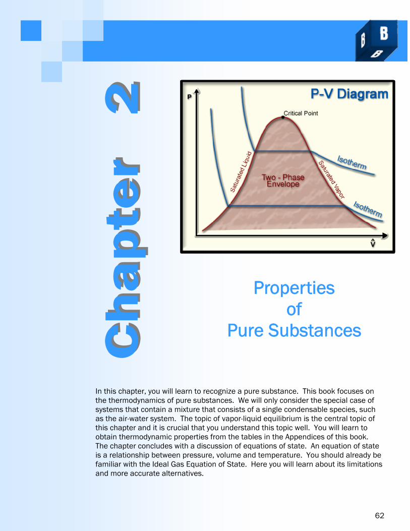
In this chapter, you will learn to recognize a pure substance. This book focuses on the thermodynamics of pure substances. We will only consider the special case of systems that contain a mixture that consists of a single condensable species, such as the air-water system. The topic of vapor-liquid equilibrium is the central topic of this chapter and it is crucial that you understand this topic well. You will learn to obtain thermodynamic properties from the tables in the Appendices of this book. The chapter concludes with a discussion of equations of state. An equation of state is a relationship between pressure, volume and temperature. You should already be familiar with the Ideal Gas Equation of State. Here you will learn about its limitations and more accurate alternatives.
Ch
ap
ter
2
Ch
ap
ter
2

Workbook LearnThermo.com Chapter 2
Properties of Pure Substances Page 63
Pure Substance Dry air is a pure substance Humid air can be considered to be a pure
substance A tank containing liquid water with humid
air above it cannot be considered to be a pure substance !
Phases Multiple liquid phases can exist in equilib-
rium: oil and water Multiple solid phases can exist in equilib-
rium: diamond and carbon, different types of ice crystals, different types of steels.
Only ONE gas phase can exist at equilib-rium. All the molecules always mix.
Phase Changes What is the difference between boiling and
evaporating ? Sublimation: Did you ever notice that old
ice cubes in your home freezer have shrunk ? Do you think they melted ? No. They sublimated !
Phase Diagrams An isobaric process path is a smooth way to
introduce Phase Diagrams Phase Diagrams are our FRIENDS…they
make any process a little easier to under-stand.
Quality: x = fraction of the mass in the systemthat exists in the gas or vapor phase.
1 – Subcooled LiquidT < Tsat and P*(T) < P and x is undefined
2 – Saturated LiquidT = Tsat and P*(T) = P and x = 0
3 – Saturated MixtureT = Tsat and P*(T) = P and 0 < x < 1
4 – Saturated VaporT = Tsat and P*(T) = P and x = 1
5 – Superheated VaporT > Tsat and P*(T) > P and x is undefined
Isobaric Heating of a Pure Substance
Nomenclature
Pure Substance Uniform chemical composition throughout the system
Phases Liquids: Multiple liquid phase
Solids: Multiple solid phases Gases: Only ONE gas phase can exist
Phase Changes
Liquid » Gas: Boiling or Evaporating / Condensing Liquid » Solid: Melting / FreezingGas » Solid: Sublimating / Desublimating
Liquid » Gas : An Isobaric Process Path Consider the isobaric process on the next slide in which energy is
added to a closed system that initially contains liquid water at a T < Tsat

Workbook LearnThermo.com Chapter 2
Page 64 Properties of Pure Substances
1
2 3 4
5
Elements of the Vapor-Liquid region of a phase diagram
Sat’d Liquid Curve Sat’d Vapor curve Critical Point Two Phase Envelope where vapor and
liquid both exist within the system at equi-librium
Subcooled liquid region Superheated vapor region Supercritical fluid region
Isobaric Heating Process Slides up and to the left along an isobar
This PV diagram extends down into the solid region
We will focus on the vapor-liquid region in this course.
Same elements in this diagram as in the TV Diagram, but they are located in slightly different positions.
Isobaric Heating Process Slides to the left along a horizontal isobar
Isothermal Heating Process Path on a PV Diagram
Isobaric Heating Process Path on a TV Diagram


2A-1 2 pts
As long as the composition remains constant and uniform throughout, a homogeneous mixture can be treated as a pure substance. We call this a pseudo-component.
Think About Tea
Tea is a mixture of one or more tasty oils dissolved in hot water. Is this a heterogeneous or homogeneous mixture? Are there any conditions under which this tea can be considered to be a pure substance? Explain.
If the tea is well-mixed, perhaps by stirring, then the mixture can be adequately described as homogeneous.
Dr. B - LearnThermo.com Ex 2A-1 Copyright B-Cubed 2014, all rights reserved

2C-3 4 pts
Read :
Given: D 0.14 m Patm 101.325 kPamlid 3.7 kg
Find: Tboil ???oC
Assumptions: None.
Equations / Data / Solve:
Eqn 1
Eqn 2
Let's begin by determining the pressure within the pot required to lift the lid. This can be accomplished by writing a force balance on the lid. See the diagram.
The lid will lift slightly and let some air escape when the upward force exerted by the gas inside the pot just balances the sum of the weight of the lid and the downward force due to atmospheric pressure on the outside of the lid.
The fact that the lid is not flat on top does not affect the solution of this problem, as long as the lid is axially symmetric about its centerline.
All of the horizontal components of the forces acting on the lid cancel each other out (vector sum is zero). The downward force is the same regardless of the shape of the top of the lid. Remember that pressure always acts in the direction perpendicular or normal to a surface. So as the lid surface curves, the downward component of the pressure force decreases. But the total surface area of the pot increases. These two factors are equal and opposite. The result is that the force exerted by the outside atmosphere on the pot lid is the same as if the lid were flat. The area of an equivalent flat surface is called the projected area (I use the symbol Aproj).
Water Boils at a Higher Temperature in a Covered Pot
A large pot has a diameter of 14 cm. It is filled with water and covered with a heavy lid that weighs 3.7 kg. At what temperature does the water begin to boil if ambient pressure is 101.325 kPa?
The key to this problem is to recognize that the total pressure at the surface of the liquid water must be greater than 101 kPa before the water can boil because of the weight of the lid. This is true whether there is an air space between the liquid water and the lid or not. As the temperature of the contents of the pot rises, the pressure will increase. When the 1st bubble of water vapor forms, it will displace some air. The displaced air will escape by lifting the lid.
The liquid water will boil when it reaches the temperature at which the vapor pressure of the water is equal to the pressure required to lift the lid and let some air escape.
P,in P,out wtF F F= +
P,out atm projF P A=
Dr. B - LearnThermo.com Ex 2C-3 Copyright B-Cubed 2014, all rights reserved

Eqn 3
The only term left is the weight of the pot lid. This is an application of Newton's 2nd Law.
Eqn 4
Eqn 5
Eqn 6
Eqn 7 Aproj 0.015394 m2
1 kPa 1000 N/m2
g 9.8066 m/s2
gc 1 kg-m/N-s2 Pin 103.68 kPa
Tsat (oC) Psat (kPa)
100.00 101.42Tboil 103.68
105.00 120.90 Interpolation yields : Tboil 100.5810 oC
Verify: None.
Answers : Tboil 100.6 oC
Following the same logic, the upward force exerted by the air in the pot on the lid can be determined using :
The goal is to determine the pressure inside the pot when the lid lifts and the water boils, so let's solve Eqn 5 for the unknown Pin.
At last, we can plug numbers into Eqn 6 and evaluate the pressure in the pot when the water boils.Just be sure to use the unit conversion :
Because 102.25 kPa is not an entry in the Saturation Pressure Table, an interpolation is required.
Now, we can substitute Eqns 2, 3 & 4 into Eqn 1 :
The only unknown quantity on the right-hand side of Eqn 6 is the projected area. We can calculate its value using :
Finally, we can go to the Saturation Pressure Table in the Steam Tables to determine the saturation pressure at Pin. This is the temperature at which the water in the pot will boil.
P,in in projF P A=
wt lidc
gF m
g=
in proj atm proj lidc
gP A P A m
g= +
lidin atm
proj c
m gP P
A g= +
2projA D
4
p=
Dr. B - LearnThermo.com Ex 2C-3 Copyright B-Cubed 2014, all rights reserved

126
Heat Effects
Ch
ap
ter
3
Ch
ap
ter
3
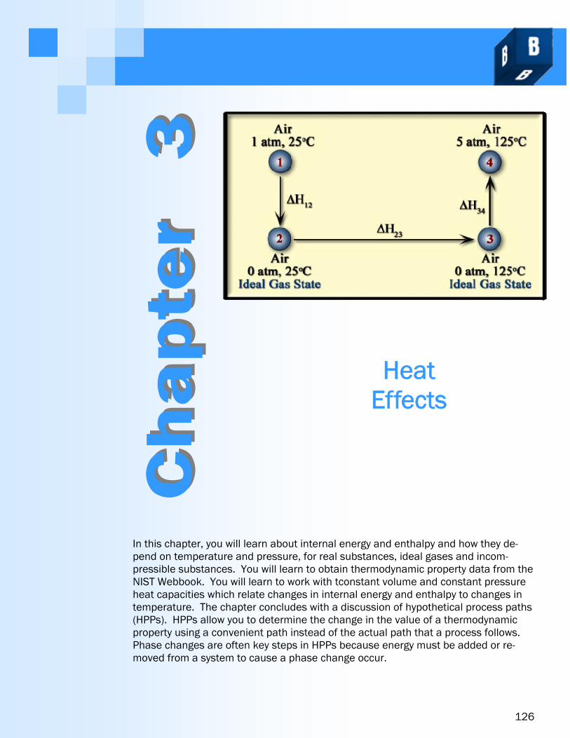
In this chapter, you will learn about internal energy and enthalpy and how they de-pend on temperature and pressure, for real substances, ideal gases and incom-pressible substances. You will learn to obtain thermodynamic property data from the NIST Webbook. You will learn to work with tconstant volume and constant pressure heat capacities which relate changes in internal energy and enthalpy to changes in temperature. The chapter concludes with a discussion of hypothetical process paths (HPPs). HPPs allow you to determine the change in the value of a thermodynamic property using a convenient path instead of the actual path that a process follows. Phase changes are often key steps in HPPs because energy must be added or re-moved from a system to cause a phase change occur.

Workbook LearnThermo.com Chapter 3
Heat Effects Page 127
Atoms are in motion in all phases, even solids
They vibrate, rotate and translate. This behavior is a strong function of tem-
perature Internal energy is a weak function of P. U
decreases slightly as P increases. At the same Temperature, Ugas > Uliq > Usolid
Special Cases Ideal Gases: U = fxn(T) only. U ≠ fxn(P) Incompressible Liquids: U = fxn(T) only.
U ≠ fxn(P) Solids: U = fxn(T) only. U ≠ fxn(P)
Enthalpy H = U + P V H = U + (PV) is NOT always the
same as H = U + PV Specific and Molar forms of this equation
are valid. For ideal gases, H ≠ fxn(P) For solids and incompressible liquids, H
is a fxn(P) H = U + (PV) = (PV) = V (P)
because V is constant !
Item 4 is VERY important ! We will always use the “Default for Fluid”
setting, unless I ask you to do otherwise. But, what is a “Standard State Conven-
tion” ? I call it a Reference State.
Internal Energy and Enthalpy
Internal Energy Isobaric – constant pressure Non-nuclear energy stored within molecules Sum of the vibrational, translational and rotational kinetic energies U = strong fxn of T and a weak fxn of P U sharply as T but U slightly as P . Ideal Gas, Incompressible Liquids, Solids U = fxn(T) only U fxn(P)
Enthalpy H = U + P V dH = dH + d(PV) H = U + (PV) H = strong fxn(T) H = moderate fxn(P) Ideal Gas: H fxn(P)S


164
The First Law of
Thermodynamics:
We begin this chapter by introducing the concepts of work and heat. This leads to the study of multi-step processes in which a system interacts with the surroundings by exchanging heat and work. When heat and work are exchanged with the surroundings, the P, V and T of the system can change. We can show the process path on a PV Diagram. Several special types of process paths are discussed in this chapter. The First Law of Thermodynamics is introduced and used to analyze processes that take place in closed systems (no mass crosses the system boundary). The chapter concludes with a discussion of heat engines and their thermal efficiency and refrigeration and heat pump cycles and their coefficients of performance.
Ch
ap
ter
4
Ch
ap
ter
4

Workbook LearnThermo.com Chapter 4
The First Law of Thermodynamics Page 165
increases as T increases, so changes in
have a natural sign.
This is not true for work A system can do work on the surroundings or the
surroundings can do work on the system We choose which is positive and which is negative.
We choose a sign convention. In this course we choose work done BY the system
on the surroundings to be positive Always include an arrow for work
on our sketches to indicate the sign convention we are using.
Sign Convention for Work
Work
Definition A force acting through a distance A restraining force is overcome to move an object
Boundary Work or PV Work: F = P A
Thermodynamic Definition of Work Work is done by a system on its surroundings if the sole effect of
a process on its surroundings could have been raising a weight. This definition allows for other forms of work, such as spring
work, electrical work, gravitational work and acceleration work.
State 2
12State1
W F dx N m J
State 2 State 2
bState1 State1
W P A dx P dV
U
System
WORK


216
The First Law of
Thermodynamics: Open Systems
Many important processes take place in open systems. Application of the First Law of Thermodynamics to an open system leads to the rate form of the First Law. The concept of flow work is introduced and this allows us to eliminate internal energy terms in favor of enthalpy terms in the First Law. The next part of Chapter 5 shows how the First Law can be used to analyze a wide variety of steady-state processes including pumps, compressors, turbines, nozzles and heat exchangers. Chapter 5 concludes with a discussion of transient or unsteady-state processes. We learn how to analyze transient uniform state, uniform flow processes.
Used by permission from Trane
Ch
ap
ter
5
Ch
ap
ter
5

Workbook LearnThermo.com Chapter 5
The First Law of Thermodynamics: Open Systems Page 217
Rate of change of mass in the system = totalrate at which mass enters the system - total rate at which mass leaves the system
A feed stream enters the system An effluent stream leaves the system These equations look complicated, but, in
practice, they are pretty simple.
The 2nd equality in the equation for volu-metric flow rate only applies to conduits with circular cross-sectional area.
Flow Rates and Velocity
Conservation of Mass
Mass is neither created nor destroyed Integral Mass Balance on an Open System
Differential Mass Balance on an Open System
Specific Volume: or:
Therefore:
Volumetric Flow Rate:
Where: <v> = average fluid velocity Across = cross-sectional area for flow
Conclusion:
#feeds #effluents
sys in,i out , ji 1 j 1
m m m
#feeds #effluents
in,i out, jsysi 1 j 1
dm m m
dt
in,1m
in,2m
in,3m
out,1m
out,2m
VV
m VV
m
Vm
V
R
cross0
V v dA 2 v dr v A
crossv AVm
ˆ ˆV V


269
The Second Law of
Thermodynamics
In this chapter, we begin with the concept of a thermal reservoir and show how they can be used in heat engines, refrigerators and heat pumps.Next, we introduce a sim-ple, intuitive statement of the Second Law of Thermodynamics. In this chapter and the next one, we develop progressively more useful statements of the Second Law. These help us understand and analyze the feasibility and performance of processes and cycles.
Next, we discuss the concept of reversibility and sources of irreversibility. The Carnot Cycle is a reversible cycle that leads to two new and important implications of the Second Law called the Carnot Principles. The Carnot Principles are used with the Kelvin Relationship to establish the fact that the Kelvin temperature scale is a thermodynamic temperature scale. This establishes a relationship between the thermal efficiency of a power cycle and the temperatures of the thermal reservoirs with which it interacts. This leads to the key idea that the usefulness or value of 1 kJ of energy depends on the temperature of the reservoir from which you take it.
Ch
ap
ter
6
Ch
ap
ter
6

Workbook LearnThermo.com Chapter 6
The Second Law of Thermodynamics Page 270
A cup of water left out on a table at roomtemperature does not spontaneously freeze unless room temperature drops below 0oC.
A cup of water left out on a table at roomtemperature does not spontaneously boil unless room temperature climbs above 100oC.
But if these things did happen, it wouldNOT VIOLATE the 1st Law !
As long as 100 kJ leaves the water and 100kJ enters the surroundings, the 1st Law is satisfied.
And yet this NEVER happens. So, the 1st Law is completely inadequate to
explain WHY these things never happen. We can take advantage of things that hap-
pen spontaneously. Don’t think of things that are not in equilib-
rium as being bad or negative. We would not be alive if we were in equi-
librium with our surroundings !
Examples of bodies that are nearly perfectthermal reservoirs include a lake, an ocean and the Earth’s atmosphere.
For practical purposes, their temperaturedoes not change because my kitchen refrig-erator is operating.
Another good example of a thermal reser-voir is a body in which phase equilibrium exists.
The temperature of an ice-water bath doesnot change as heat is transferred into the bath.
Instead the heat transferred supplies thelatent heat of fusion required to melt some of the ice.
Thermal Reservoirs and Cycles
1st Law and Spontaneity
1st Law: Energy is neither created nor destroyed Places no restriction on the direction that energy flows sponta-
neously Imagine a cup of water rejecting 100 kJ to the surrounding air and
freezing solid. Imagine a cup of water absorbing 100 kJ from the surrounding air and
boiling. We need another law to help us understand why these things do
not happen spontaneously. Spontaneity
Unbalanced forces tend to drive the state of a system towards an equilibrium state
We can harness these unbalanced driving forces to do work for us.
The greater the unbalanced driving force, the greater thepotential to do work.
Thermal Reservoirs Bodies than can exchange an infinite
amount of heat, but the temperature of the thermal reservoir never changes.
Heat Sink: Reservoir that absorbs heat Heat Source: Reservoir that puts out
heat Types of Thermodynamic Cycles
Power Cycle Purpose: produce WS, Input: QH, Waste: QC
Refrigeration Cycle Purpose: produce QC, Input: WS, Waste: QH
Heat Pump Cycle Purpose: produce QH, Input: WS, Waste: QC
Hot Reservoir
Cold Reservoir
Cycle


316
Entropy
In this chapter, we use the Kelvin Relationship and the Carnot Pricniples to show that the Clausius Inequality is true. This leads to the definition of entropy. The TS Diagram will be used frequently in the remainder of this course because it provides a great deal of insight into the performance of processes and cycles. The Principle of Increasing Entropy leads to the concept of entropy generation.
The 1st and 2nd Gibbs Equations are introduced to facilitate the evaluation of changes in entropy associated with processes. We apply the Gibbs equations to incompressible liquids and ideal gases. This analysis leads to the Ideal Gas Entropy Function and to relative properties. These are tabulated in the Appendix.
The chapter concludes with a discussion of polytropic, isentropic and other special processes and their representation on PV and TS Diagrams.
Ch
ap
ter
7
Ch
ap
ter
7

Workbook LearnThermo.com Chapter 7
Entropy Page 317
Cyclic integrals are new, but they are not scaryor terribly difficult when applied to thermody-namic cycles.
All you need to do is integrate through all thesteps of the cycle, so that you begin and end in the same state.
The funky “” is a common way of indicatingthat the differential is not an exact differential, “”, nor is it a partial differential, “¶”.
It is absolutely crucial that you understand thesetwo examples of how to evaluate a cyclic inte-gral.
Example 1 In the cyclic integral, our sign convention applies,
but in the tie-fighter diagram, both QH and QC are positive quantities.
When we evaluate the cyclic integral, we get some-thing like Q12 + Q23 + Q34 + Q41 for a Carnot cycle.
In a Carnot Cycle, Steps 2-3 and 4-1 are adiabatic, so Q23 = Q41 = 0.
So, the cyclic integral is just Q12 + Q34 . Because of the sign convention conflict, QH = Q12
and QC = - Q34 . Therefore, the cyclic integral is QH – QC . The 1st Law tells us that QH = QC + WHE Since WHE > 0, QH > QC and finally
QH – QC > 0
Reversible Cycles Kelvin Relationship applies to reversible cycles like
Carnot Depends on the fact that the temperature scale we
use, the Kelvin Scale, is a thermodynamic tem-perature scale
Irreversible Cycles: Consider an irreversible HE that operates be-
tween the same hot and cold thermal reservoirs and receives the same amount of heat from the hot reservoir, QH.
1st Carnot Principle : the reversible HE is more efficient than the irreversible HE
Thermal efficiency is defined as the ratio of the work output to QH. Since QH is the same for both HE’s and the effi-
ciency of the reversible HE is greater, we con-clude that the work output of the irreversible HE must be less than the work output of the reversible HE.
The 1st Law allows us to replace the work output with QH – QC for each HE.
The QHterm on each side of the inequality cancels leaving us with the fact that the irreversible HE must reject more heat to the cold reservoir than the re-versible HE does.
The Cyclic Integral We can now apply the cyclic integral of dQ/T to
the irreversible process. The key here is that we can use the Kelvin Rela-
tionship (applied to the reversible HE, not this irreversible one) to replace QH / TH with QC,rev / TC .
We just showed that QC,rev < QC,irr , so we con-clude that the cyclic integral must be negative for all irreversible cycles !
Clausius: Int. Rev. and Irrev. Cycles
The Clausius Inequality
Cyclic Integrals Integrate through all the steps in
a cycle and return to the initial state. Inexact Differentials: Q & W
Used for path variables, Q and W Evaluating Cyclic Integrals
Example 1: Carnot HE
Example 2: Carnot HE
Hot Reservoir
Cold Reservoir
HER
QH
QC,rev Wrev
Q0
T
2 4
12 34 H C1 3
Q Q Q Q Q Q Q 0
42
2 4C,rev3 341 12 H
H C H C H C1 3
QQQQQ QQ Q Q
T T T T T T T T T
Reversible Cycle, such as Carnot:
Kelvin: or:
Therefore:
Irreversible Cycles: Definition of efficiency : 1st Law :
Hot Reservoir
Cold Reservoir
HEIr
QH
QC,irr Wirr
All Cycles :
C,revH
H C
QQQ
T T T
C,rev H
C H
Q Q
T TC,rev C
H H
Q T
Q T
Q0
T
rev irr
rev irrW W
H C ,rev H C ,irrQ Q Q Q
C ,rev C ,irrQ Q
C,irr C,rev C,irrirr H
H C C C
Q Q QQ Q0
T T T T T
Q0
T
Example 2 Because the Carnot Cycle is completely reversible, all heat transfer must occur through an
infinitessimal temperature difference. Therefore, the temperature of the hot reservoir must be equal to the temperature of the
working fluid in the system to which it transfers heat. And the temperature of the cold reservoir must be equal to the temperature of the working
fluid in the system from which it receives heat. Since the reservoir temperatures are constant, the temperatures within the system where the
heat exchange occurs must also be constant.
Conclusions The Clausius Inequality is TRUE ! The equality applies for int. rev. cycles and the “less
than” part applies for irreversible cycles. Why relax the rule from reversible to just internally reversible ? If the temperatures inside
the system are NOT equal to the temperatures of the hot and cold reservoirs, then the heat exchange is NOT reversible.
But, the Kelvin Relationship applies if the cycle is internally reversible. As long as the cycle is internally reversible, the equality in the Clausius Inequality applies. The temperature within the system at which heat exchange occurs does not need to be con-
stant for the equality part of Clausius to hold true. It just makes it a WHOLE LOT easier to evaluate the cyclic integral.


380
Thermodynamics of
Flow Processes
The concept of entropy generation allows us to write entropy balance equations for both closed and open systems. Combination of the 1st and 2nd Laws and the 2nd Gibbs Equation leads to the Mechanical Energy Balance Equation, the Bernoulli Equation and a surprising relationship between shaft work, pressure and volume. Equations are derived for the shaft work of various polytropic processes.
This leads to the definition of isentropic efficiencies for turbines, nozzles and compressors. Isentropic efficiency is best visualized on an HS Diagram. Multi-stage compression with intercooling is discussed and represented on an HS Diagram.
The utility of the concept of entropy generation lies in its relationship to lost work. Equations relating entropy generation to lost work are derived for processes and cycles. Second Law Efficiency of a process is defined and discussed.
Ch
ap
ter
8
Ch
ap
ter
8

Workbook LearnThermo.com Chapter 8
Thermodynamics of Flow Processes Page 381
We start with closed systems, just to bethorough. The interesting application of the 2nd Law is for open systems.
This is a quick run down of all the equa-tions that apply to closed systems.
The new part is the entropy balance equa-tion. The integral form is the one we will use
most for closed systems. It is essentially the definition of entropy
generation. It is not really new.
The rate form is a nice lead in to entropy balances on open systems.
The general form of the entropy balanceequation states that the entropy of the sys-tem changes for four different reasons. Mass entering and leaving the system
carries entropy with it. The rate at which the entropy of the
system changes as a result is equal to the rate at which mass flow carries en-tropy into the system minus the rate at which mass flow carries entropy out of the system.
Heat transfer to and from the system re-sults in a change in the entropy of the sys-tem. Each place in the system where heat
transfer occurs changes the entropy of the system at a rate of Qdot / T , where T is the temperature of the system at the particular location where heat transfer occurs.
The net rate at which heat transferchanges the entropy of the system is the sum of all the individual Qdot / T terms.For example: QH / Tsys,H – QC / Tsys,C for a heat engine with an evapora-tor operating at Tsys,H and a condenser operating at Tsys,C .
Note: These T’s are the temperatures withinthe system and NOT the temperatures of the
Entropy Balance: Open System
Entropy Balance: Closed System
1st Law:
2nd Law, InternallyReversible Processes:
Boundary Work, InternallyReversible Processes:
Gibbs 1st Equation:
Entropy Balance Equation
Integral Form:
Differential Form:
Rate Form:
Steady-state, SISO:
General:
Entropygeneration within the system: gen out in
sys
Qˆ ˆS m S ST
genout insys
Qˆ ˆm S S ST
inlets outletssys
in out genin outsys
dS Qˆ ˆm S m S Sdt T
gendS Q
Sdt T
gen
QdS S
T
2
2 1 gen1
QS S S
T
dU T dS p dV
bW P dV
Q T dS
dU Q W
The general entropy balance equation can be simplified a great deal for aSISO system operating at steady-state.
Often, our objective is to determine the rate of entropy generation in a sys-tem. You will see why this is a key quantity later in this chapter.
It is very important to realize that this is ONLY the entropy generationwithin the system.
What about the reservoirs and the surroundings ? Irreversible heat exchange leads to additional external entropy generation.


440
Power Systems
This chapter focuses on practical aspects of power generation using heat engines. In particular, we look at how the efficiency of power cycles can be increased.
The first part of the chapter covers the Rankine vapor power cycle. Five variations on the Rankine Cycle that increase the thermal efficiency of the cycle are discussed in detail.
In the second half of this chapter, gas power cycles are discussed. Many gas power cycles exist, but we limit our discussion to the Air-Standard Brayton Power Cycle. Four variations on the Air-Standard Brayton Power Cycle that increase the thermal efficiency of the cycle are discussed.
The impact of process irreversibilties on the thermal efficiencies of these cycles are also discussed.
Ch
ap
ter
9
Ch
ap
ter
9

Workbook LearnThermo.com Chapter 9
Power Systems Page 441
Power systems use a high-temperature heatsource to produce work, usually shaft work.
So far, we have only discussed closed cy-cles. The working fluid is recycled. Open cycles are often used in transporta-
tion systems, such as cars and planes. The working fluid is almost always air. This type of cycle eliminates the heat
exchanger in which the working fluid is cooled or condensed to complete the cycle and return to the original state.
Instead, fresh working fluid is drawninto the system put through 3 steps of the cycle and then flows out of the sys-tem.
Think of automobile exhaust or jet en-gine contrails and you will have the right idea.
We will model open cycles as if theywere really closed cycles.
◊ This makes it easier to see the similarities between cycles. ◊ It also simplifies the analysis some- what. ◊ More about open cycles in Lessons
9E & 9F.
We learned in Ch 8 that for internally re-versible, SISO processes operating at steady-state with negligible changes in ki-netic and potential energies… The specific shaft work for a process is
minus the integral of V^ dP. We apply this to each of the four processes
that make up a Carnot Cycle and find that… The area enclosed by the cycle path is
equal to the specific shaft work produced by the cycle.
Remember that power cycles proceed clockwise around the cycle path on PV Diagrams.
PV Diagram: Power Cycles
Vapor and Gas Power Systems
Vapor Cycles
Use evaporator and condenser for isothermal heat transfer steps Gas Cycles
No phase changes Use isobaric heat exchangers for heat transfer steps
Closed Cycles Not piston-and-cylinder devices Working fluid remains inside the system Use two HEX’s to absorb and reject heat Power generation turbines
Open Cycles Fresh working fluid drawn into the cycle Spent working fluid discarded after 1 pass through the cycle Usually air is the working fluid Only 1 HEX because the fluid doesn’t actually complete the cycle
Automobile and jet engines
In Vapor or Gas Power Cycles, the area enclosed bythe cycle path is equal to the specific shaft work pro-duced by the cycle.
This is a PV Diagram of aGas Power Cycle
A Vapor Power Cycle looksthe same, but the 2-phase envelope is also shown on the plot.
2 3 4 1Sh ,cycle
1 2 3 4
W ˆ ˆ ˆ ˆV dP V dP V dP V dP Enclosed Aream
P
V
QH
QC
1
2
3 4
TH
TC


488
Refrigeration and
Heat Pump Systems
In this chapter, we discuss refrigeration and heat pump systems in a manner analo-gous to our discussion of power systems in Chapter 9.
We begin with a discussion of ideal vapor-compression refrigeration (VCR) and follow with a discussion of the impact of irreversibilities on the coefficient of performance. Refrigerant selection criteria are discussed, with special attention to the vapor pres-sure—temperature relationship. Cascade and multi-stage VCR cycles are covered. Heat pumps and the key reversing valve are discussed.
The chapter concludes with a discussion of Air-Standard Gas Refrigeration Cycles. Regeneration can be used to increase the coefficient of performance. Irreversibilities decrease the coefficient of performance.
Ch
ap
ter
10
Ch
ap
ter
10

Workbook LearnThermo.com Chapter 10
Refrigeration and Heat Pump Systems Page 489
Refrigeration revolutionized fooddistribution.
◊Limits the growth of bacteria in the food supply.
Air-conditioning dramatically improved lifein the tropical and subtropical regions. Facilitated the economic development of the
southern US. Gas refrigeration is not as efficient as V-C
refrigeration. But, it is lightweight. This makes it well-
suited to use in passenger aircraft. The other great attribute of gas refrigeration
cycles is that they can reach very, very low temperatures, even into the cryogenic range.
Thermoelectric refrigerators make use ofthe Peltier Effect. When a current is passed through the junction
between two wires made of different metals, heat is either released or absorbed, depending on the direction of the electrical current.
This is also the principle upon which thermo-couples operate.
Thermoelectric refrigerators are lightweight and inexpensive, but not very efficient. (Less than 10% of Carnot Efficiency, so generally less than 5%.)
Harrison Ford builds a giant ammonia ab-sorption refrigeration system in the film Mosquito Coast !
The refrigeration system in the VW Euro-van and most campers is an ammonia re-frigeration system! It is VERY important to park the Eurovan
or camper on level ground in order to make the refrigerator work.
See why by visiting the Ammonia Refrig-eration Technicians Association website.
Ammonia Absorption Refrigeration
Applications of Refrigeration Systems
V-C Refrigeration Cycle Food preservation Air conditioning Industrial cooling processes
Gas Refrigeration Cycle Air conditioning on passenger aircraft Cryogenic refrigeration (very low temperatures, < 150 K)
Thermoelectric Refrigeration Systems Peltier Effect Very small and lightweight
Very low efficiency
Ammonia Absorption Refrigeration No moving parts No work input Well-suited to remote and portable applications
Locations where electric power is not available
RV’s and campers Invented by a student in Sweden
See external flow diagram or visit:http://www.nh3tech.org/absorption.html

Workbook LearnThermo.com Chapter 10
Page 490 Refrigeration and Heat Pump Systems
The ideal VCR Cycle is not internallyreversible because flow through the expansion valve has lots of friction and is therefore irreversible.
Notice that the expansion valve (step 4-1) isNOT isentropic !
◊There is a great deal of friction in athrottling device.
◊Lots of irreversibility. ◊Lots of lost work ! ◊The expansion valve is isenthalpic.
The evaporator effluent is saturated vapor.
Ideal VCR Cycle: TS Diagram
Ideal V-C Refrigeration Cycle The Ideal V-C Refrigeration Cycle
Step 1-2: Evaporator Heat absorbed at constant pressure Step 2-3 Compressor Isentropic compression Step 3-4: Condenser Heat rejected at constant pressure Step 4-1: Expansion Valve Isenthalpic expansion
C 2 1R
cycle 3 2
ˆ ˆH HQCOP
ˆ ˆH HW

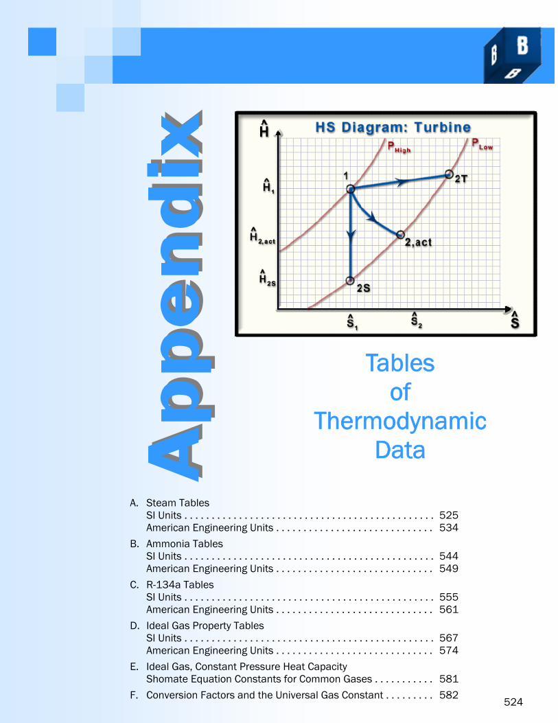
524
Tables of
Thermodynamic Data
A. Steam Tables SI Units . . . . . . . . . . . . . . . . . . . . . . . . . . . . . . . . . . . . . . . . . . . . . . 525 American Engineering Units . . . . . . . . . . . . . . . . . . . . . . . . . . . . . 534
B. Ammonia Tables SI Units . . . . . . . . . . . . . . . . . . . . . . . . . . . . . . . . . . . . . . . . . . . . . . 544 American Engineering Units . . . . . . . . . . . . . . . . . . . . . . . . . . . . . 549
C. R-134a Tables SI Units . . . . . . . . . . . . . . . . . . . . . . . . . . . . . . . . . . . . . . . . . . . . . . 555 American Engineering Units . . . . . . . . . . . . . . . . . . . . . . . . . . . . . 561
D. Ideal Gas Property Tables SI Units . . . . . . . . . . . . . . . . . . . . . . . . . . . . . . . . . . . . . . . . . . . . . . 567 American Engineering Units . . . . . . . . . . . . . . . . . . . . . . . . . . . . . 574
E. Ideal Gas, Constant Pressure Heat Capacity Shomate Equation Constants for Common Gases . . . . . . . . . . . 581
F. Conversion Factors and the Universal Gas Constant . . . . . . . . . 582
Ap
pe
nd
ixA
pp
en
dix

Workbook LearnThermo.com Appendix A
Saturation Temperature Table WaterSI
Sat. Liq Sat. Vap Sat. Liq Sat. Vap Sat. Liq Sat. Vap Sat. Liq Sat. Vap
0.01 0.61165 0.0010002 205.99 0 2374.9 6.1178E-04 2500.9 0 9.15555 0.87258 0.0010001 147.01 21.019 2381.8 21.020 2510.1 0.076254 9.0248
10 1.2282 0.0010003 106.30 42.020 2388.6 42.021 2519.2 0.15109 8.899815 1.7058 0.0010009 77.875 62.980 2395.5 62.981 2528.3 0.22446 8.780320 2.3393 0.0010018 57.757 83.912 2402.3 83.914 2537.4 0.29648 8.666025 3.1699 0.0010030 43.337 104.83 2409.1 104.83 2546.5 0.36722 8.556630 4.2470 0.0010044 32.878 125.73 2415.9 125.73 2555.5 0.43675 8.452035 5.6290 0.0010060 25.205 146.63 2422.7 146.63 2564.5 0.50513 8.351740 7.3849 0.0010079 19.515 167.53 2429.4 167.53 2573.5 0.57240 8.255545 9.5950 0.001009950 12.352 0.001012155 15.762 0.001014660 19.946 0.001017165 25.042 0.001019970 31.201 0.001022875 38.595 0.001025880 47.414 0.001029185 57.867 0.001032490 70.182 0.001036095 84.608 0.0010396
100 101.42 0.0010435105 120.90 0.0010474110 143.38 0.0010516115 169.18 0.0010559120 198.67 0.0010603125 232.24 0.0010649130 270.28 0.0010697135 313.23 0.0010746140 361.54 0.0010798145 415.68 0.0010850150 476.16 0.0010905155 543.50 0.0010962160 618.23 0.0011020165 700.93 0.0011080170 792.19 0.0011143175 892.60 0.0011207180 1002.8 0.0011274185 1123.5 0.0011343190 1255.2 0.0011415195 1398.8 0.0011489200 1554.9 0.0011565205 1724.3 0.0011645210 1907.7 0.0011727215 2105.8 0.0011813220 2319.6 0.0011902225 2549.7 0.0011994230 2797.1 0.0012090235 3062.5 0.0012190
Reference States: U = 0 and S = 0 at for saturated liquid at the triple point (0.01oC and 0.61165 kPa).
Temp.
(oC)Pressure
(kPa)
Page 525
S (kJ/kg*K)V (m3/kg) U (kJ/kg) H (kJ/kg)

Workbook LearnThermo.com Appendix A
Saturation Temperature Table WaterSI
Sat. Liq Sat. Vap Sat. Liq Sat. Vap Sat. Liq Sat. Vap Sat. Liq Sat. Vap
240 3346.9 0.0012295 0.059705 1033.4 2603.1 1037.6 2803.0 2.7020 6.1423245 3651.2 0.0012403 0.054654 1057.0 2602.7 1061.5 2802.2 2.7478 6.1072250 3976.2 0.0012517 0.050083 1080.8 2601.8 1085.8 2800.9 2.7935 6.0721255 4322.9 0.0012636 0.045938 1104.8 2600.5 1110.2 2799.1 2.8392 6.0369260 4692.3 0.0012761 0.042173 1129.0 2598.7 1135.0 2796.6 2.8849 6.0016265 5085.3 0.0012892 0.038746 1153.4 2596.5 1160.0 2793.5 2.9307 5.9661270 5503.0 0.0013030275 5946.4 0.0013175280 6416.6 0.0013328285 6914.7 0.0013491290 7441.8 0.0013663295 7999.1 0.0013846300 8587.9 0.0014042305 9209.4 0.0014252310 9865.1 0.0014479315 10556 0.0014724320 11284 0.0014990325 12051 0.0015283330 12858 0.0015606335 13707 0.0015967340 14601 0.0016376345 15541 0.0016846350 16529 0.0017400355 17570 0.0018079360 18666 0.0018954365 19821 0.0020172370 21044 0.0022152
373.95 22064 0.0031056
Reference States: U = 0 and S = 0 at for saturated liquid at the triple point (0.01oC and 0.61165 kPa).
Page 526
Temp.
(oC)Pressure
(kPa)V (m3/kg) U (kJ/kg) H (kJ/kg) S (kJ/kg*K)

Workbook LearnThermo.com Appendix A
Saturation Pressure Table WaterSI
Sat. Liq Sat. Vap Sat. Liq Sat. Vap Sat. Liq Sat. Vap Sat. Liq Sat. Vap
1.0 6.970 0.0010001 129.18 29.298 2384.5 29.299 2513.7 0.10591 8.97491.5 13.02 0.0010007 87.958 54.681 2392.8 54.683 2524.7 0.19556 8.82702.0 17.49 0.0010014 66.987 73.426 2398.9 73.428 2532.9 0.26056 8.72262.5 21.08 0.0010021 54.240 88.417 2403.8 88.420 2539.4 0.31182 8.64203.0 24.08 0.0010028 45.653 100.97 2407.9 100.98 2544.8 0.35429 8.57644.0 28.96 0.0010041 34.791 121.38 2414.5 121.39 2553.7 0.42239 8.47345.0 32.87 0.0010053 28.185 137.74 2419.8 137.75 2560.7 0.47620 8.39387.5 40.29 0.0010080 19.233 168.74 2429.8 168.75 2574.0 0.57627 8.250110 45.81 0.0010103 14.670 191.80 2437.2 191.81 2583.9 0.64920 8.148815 53.97 0.0010140 10.020 225.93 2448.0 225.94 2598.3 0.75486 8.007120 60.06 0.0010172 7.6480 251.40 2456.0 251.42 2608.9 0.83202 7.907225 64.96 0.0010198 271.93 2462.4 271.96 2617.4 0.89319 7.830230 69.10 0.001022240 75.86 0.001026450 81.32 0.001029975 91.76 0.0010372
100 99.61 0.0010432125 106.0 0.0010482150 111.3 0.0010527175 116.0 0.0010568200 120.2 0.0010605225 124.0 0.0010640250 127.4 0.0010672275 130.6 0.0010703300 133.5 0.0010732325 136.3 0.0010759350 138.9 0.0010786375 141.3 0.0010811400 143.6 0.0010836450 147.9 0.0010882500 151.8 0.0010925550 155.5 0.0010967600 158.8 0.0011006650 162.0 0.0011044700 164.9 0.0011080750 167.7 0.0011114800 170.4 0.0011148850 172.9 0.0011180900 175.4 0.0011212950 177.7 0.00112421000 179.9 0.00112721100 184.1 0.00113301200 188.0 0.00113851300 191.6 0.00114381400 195.0 0.00114891500 198.3 0.00115391750 205.7 0.00116572000 212.4 0.0011767
Reference States: U = 0 and S = 0 at for saturated liquid at the triple point (0.01oC and 0.61165 kPa).
S (kJ/kg*K)V (m3/kg) U (kJ/kg) H (kJ/kg)Pressure(kPa)
Temp.
(oC)
Page 527

Workbook LearnThermo.com Appendix A
Saturation Pressure Table WaterSI
Sat. Liq Sat. Vap Sat. Liq Sat. Vap Sat. Liq Sat. Vap Sat. Liq Sat. Vap
2250 218.41 0.0011873 0.088715 933.57 2600.9 936.24 2800.5 2.5029 6.29542500 223.95 0.0011974 0.079949 958.91 2602.1 961.91 2801.9 2.5543 6.25583000 233.85 0.0012167 0.066664 1004.7 2603.2 1008.3 2803.2 2.6455 6.18563500 242.56 0.0012350 6.12434000 250.35 0.0012526 6.06965000 263.94 0.0012864 5.97376000 275.58 0.0013193 5.89017000 285.83 0.0013519 5.81488000 295.01 0.0013847 5.74509000 303.34 0.0014181 5.6791
10000 311.00 0.0014526 5.616011000 318.08 0.0014885 5.554512000 324.68 0.0015263 5.493913000 330.85 0.0015665 5.433614000 336.67 0.0016097 5.372715000 342.16 0.0016570 5.310616000 347.35 0.0017094 5.246317000 352.29 0.0017693 5.178718000 356.99 0.0018398 5.106119000 361.47 0.0019268 5.025620000 365.75 0.0020400 4.931421000 369.83 0.0022055 4.807922000 373.71 0.0027044 4.544622064 373.95 0.0031056 4.4070
Reference States: U = 0 and S = 0 at for saturated liquid at the triple point (0.01oC and 0.61165 kPa).
Page 528
Pressure(MPa)
Temp.
(oC)V (m3/kg) U (kJ/kg) H (kJ/kg) S (kJ/kg*K)

Workbook LearnThermo.com Appendix A
Superheated Vapor WaterSI
Temp.
(oC)
V
(m3/kg)
U(kJ/kg)
H(kJ/kg)
S(kJ/kg*K)
V
(m3/kg)
U(kJ/kg)
H(kJ/kg)
S(kJ/kg*K)
V
(m3/kg)
U(kJ/kg)
H(kJ/kg)
S(kJ/kg*K)
Sat 14.670 2437.16 2583.9 8.148850 14.867 2443.3 2592.0 8.1741
100 17.196 2515.5 2687.5 8.4489150 19.513 2587.9 2783.0 8.6892200 21.826 2661.3 2879.6 8.9049250 24.136 2736.1 2977.4 9.1015300 26.446 2812.3 3076.7 9.2827400 31.063 2969.3 3279.9 9.6094500 35.680 3132.9 3489.7 9.8998600 40.296 3303.3 3706.3 10.163700 44.911 3480.8 3929.9 10.406800 49.527 3665.3 4160.6 10.631900 54.142 3856.9 4398.3 10.843
1000
Temp.
(oC)
V
(m3/kg)
U(kJ/kg)
H(kJ/kg)
S(kJ/kg*K)
V
(m3/kg)
U(kJ/kg)
H(kJ/kg)
S(kJ/kg*K)
V
(m3/kg)
U(kJ/kg)
H(kJ/kg)
S(kJ/kg*K)
Sat 0.60576 2543.2 2724.9 6.9916150 0.63401 2571.0 2761.2 7.0791200 0.71642 2651.0 2865.9 7.3131250 0.79644 2728.9 2967.9 7.5180300 0.87534 2807.0 3069.6 7.7037400 1.0315 2966.0 3275.5 8.0347500 1.1867 3130.6 3486.6 8.3271600 1.3414 3301.6 3704.0 8.5914700 1.4958 3479.5 3928.2 8.8344800 1.6500 3664.3 4159.3 9.0604900 1.8042 3856.0 4397.3 9.2724
1000 1.9582 4054.5 4642.0 9.4726
Temp.
(oC)
V
(m3/kg)
U(kJ/kg)
H(kJ/kg)
S(kJ/kg*K)
V
(m3/kg)
U(kJ/kg)
H(kJ/kg)
S(kJ/kg*K)
V
(m3/kg)
U(kJ/kg)
H(kJ/kg)
S(kJ/kg*K)
Sat 0.24034 2576.0 2768.3 6.6616200 0.26088 2631.0 2839.7 6.8176250 0.29320 2715.9 2950.4 7.0401300 0.32416 2797.5 3056.9 7.2345400 0.38428 2960.2 3267.6 7.5734500 0.44332 3126.6 3481.3 7.8692600 0.50185 3298.7 3700.1 8.1354700 0.56011 3477.2 3925.3 8.3794800 0.61820 3662.4 4157.0 8.6061900 0.67619 3854.5 4395.5 8.8185
1000 0.73411 4053.2 4640.5 9.0189
Reference States: U = 0 and S = 0 at for saturated liquid at the triple point (0.01oC and 0.61165 kPa).
P = 10 kPa (Tsat = 45.81oC)
P = 40 kPa (Tsat = 143.6oC)
P = 100 kPa (Tsat = 99.61oC) P = 50 kPa (Tsat = 81.32oC)
P =300 kPa (Tsat = 133.5oC)
P = 500 kPa (Tsat = 151.8oC) P = 600 kPa (Tsat = 158.8oC) P = 800 kPa (Tsat = 170.4oC)
Page 529
P = 200 kPa (Tsat = 120.2oC)
58.758 4055.2 4642.8 11.043

Workbook LearnThermo.com Appendix A
Superheated Vapor WaterSI
Temp.
(oC)
V
(m3/kg)
U(kJ/kg)
H(kJ/kg)
S(kJ/kg*K)
V
(m3/kg)
U(kJ/kg)
H(kJ/kg)
S(kJ/kg*K)
V
(m3/kg)
U(kJ/kg)
H(kJ/kg)
S(kJ/kg*K)
Sat 0.14078 2591.8 2788.8 6.4675200 0.14303 2602.7 2803.0 6.4975250 0.1635608 2698.9 2927.9 6.7488300 0.18232 2785.7 3040.9 6.9552400 0.21782 2953.1 3258.1 7.3046500 0.25216 3121.8 3474.8 7.6047600 0.28597 3295.1 3695.4 7.8730700 0.31951 3474.4 3921.7 8.1183800 0.35287 3660.2 4154.3 8.3457900 0.38614 3852.7 4393.3 8.5587
1000 0.41933 4051.7 4638.8 8.7594
Temp.
(oC)
V
(m3/kg)
U(kJ/kg)
H(kJ/kg)
S(kJ/kg*K)
V
(m3/kg)
U(kJ/kg)
H(kJ/kg)
S(kJ/kg*K)
V
(m3/kg)
U(kJ/kg)
H(kJ/kg)
S(kJ/kg*K)
Sat 0.0995851 2599.1 2798.3 6.3390250 0.11150 2680.2 2903.2 6.5475300 0.12551 2773.2 3024.2 6.7684400 0.15121 2945.9 3248.3 7.1292500 0.17568 3116.9 3468.2 7.4337600 0.19961 3291.5 3690.7 7.7043700 0.22326 3471.6 3918.2 7.9509800 0.24674 3658.0 4151.5 8.1790900 0.27012 3850.9 4391.1 8.3925
1000 0.29342 4050.2 4637.0 8.5936
Temp.
(oC)
V
(m3/kg)
U(kJ/kg)
H(kJ/kg)
S(kJ/kg*K)
V
(m3/kg)
U(kJ/kg)
H(kJ/kg)
S(kJ/kg*K)
V
(m3/kg)
U(kJ/kg)
H(kJ/kg)
S(kJ/kg*K)
Sat 0.066664 2603.2 2803.2 6.1856250 0.070627 2644.7 2856.5 6.2893300 0.081179 2750.8 2994.3 6.5412400 0.099379 2933.5 3231.7 6.9234500 0.11620 3108.6 3457.2 7.2359600 0.13245 3285.5 3682.8 7.5103700 0.14841 3467.0 3912.2 7.7590800 0.16420 3654.3 4146.9 7.9885900 0.17988 3847.9 4387.5 8.2028
1000 0.19549 4047.7 4634.1 8.4045
Temp.
(oC)
V
(m3/kg)
U(kJ/kg)
H(kJ/kg)
S(kJ/kg*K)
V
(m3/kg)
U(kJ/kg)
H(kJ/kg)
S(kJ/kg*K)
V
(m3/kg)
U(kJ/kg)
H(kJ/kg)
S(kJ/kg*K)
Sat 0.049776 2601.7 2800.8 6.0696300 0.058870 2726.2 2961.7 6.3639400 0.073431 2920.7 3214.5 6.7714500 0.086442 3100.3 3446.0 7.0922600 0.098859 3279.4 3674.9 7.3705700 0.11098 3462.4 3906.3 7.6214800 0.12292 3650.6 4142.3 7.8523900 0.13476 3844.8 4383.9 8.0674
1000 0.14652 4045.1 4631.2 8.2697
Reference States: U = 0 and S = 0 at for saturated liquid at the triple point (0.01oC and 0.61165 kPa).
P = 2500 kPa (Tsat = 224.0oC) P = 3000 kPa (Tsat = 233.9oC) P = 3500 kPa (Tsat = 242.6oC)
Page 530
P = 4000 kPa (Tsat = 250.4oC) P = 4500 kPa (Tsat = 257.4oC) P = 5000 kPa (Tsat = 263.9oC)
P = 1600 kPa (Tsat = 201.4oC)
P = 1000 kPa (Tsat = 179.9oC)
P = 2000 kPa (Tsat = 212.4oC)
P = 1400 kPa (Tsat = 195.0oC) P = 1200 kPa (Tsat = 188.0oC)
P = 1800 kPa (Tsat = 207.1oC)

Workbook LearnThermo.com Appendix A
Superheated Vapor WaterSI
Temp.
(oC)
V
(m3/kg)
U(kJ/kg)
H(kJ/kg)
S(kJ/kg*K)
V
(m3/kg)
U(kJ/kg)
H(kJ/kg)
S(kJ/kg*K)
V
(m3/kg)
U(kJ/kg)
H(kJ/kg)
S(kJ/kg*K)
Sat 0.027378 2581.0 2772.6 5.8148300 0.029492 2633.5 2839.9 5.9337400 0.039958 2879.5 3159.2 6.4502500 0.048157 3074.3 3411.4 6.8000600 0.055665 3260.9 3650.6 7.0910700 0.062850 3448.3 3888.2 7.3486800 0.069855 3639.5 4128.4 7.5836900 0.076750 3835.7 4373.0 7.8014
1000 0.083571 4037.5 4622.5 8.0055
Temp.
(oC)
V
(m3/kg)
U(kJ/kg)
H(kJ/kg)
S(kJ/kg*K)
V
(m3/kg)
U(kJ/kg)
H(kJ/kg)
S(kJ/kg*K)
V
(m3/kg)
U(kJ/kg)
H(kJ/kg)
S(kJ/kg*K)
Sat 0.020490 2558.5 2742.9 5.6791 0.0103384 2455.6 2610.7 5.3106350 0.025816 2724.9 2957.3 6.0380400 0.029960 2849.2 3118.8 6.2876 0.015671 2740.6 2975.7 5.8819500 0.036793 3056.3 3387.4 6.6603 0.020827 2998.4 3310.8 6.3480600 0.042861 3248.4 3634.1 6.9605 0.024921 3209.3 3583.1 6.6796700 0.048589 3438.8 3876.1 7.2229 0.028621 3409.8 3839.1 6.9572800 0.054132 3632.0 4119.1 7.4606 0.032121 3609.2 4091.1 7.2037900 0.059562 3829.6 4365.7 7.6802 0.035503 3811.2 4343.7 7.4288
1000 0.064918 4032.4 4616.7 7.8855 0.038808 4017.1 4599.2 7.6378
Temp.
(oC)
V
(m3/kg)
U(kJ/kg)
H(kJ/kg)
S(kJ/kg*K)
V
(m3/kg)
U(kJ/kg)
H(kJ/kg)
S(kJ/kg*K)
V
(m3/kg)
U(kJ/kg)
H(kJ/kg)
S(kJ/kg*K)
Sat
400 0.0019108 1854.9 1931.4 4.1145 0.0016329500 0.0056231 2681.6 2906.5 5.4744 0.0029522600 0.0080891 3026.8 3350.4 6.0170 0.0048330700 0.0099297 3282.0 3679.1 6.3740 0.0062649800 0.011521 3511.8 3972.6 6.6612 0.0074560900 0.012980 3733.3 4252.5 6.9106 0.0085188
1000 0.014360 3952.9 4527.3 7.1355 0.0095043
Reference States: U = 0 and S = 0 at for saturated liquid at the triple point (0.01oC and 0.61165 kPa).
P = 20000 kPa (Tsat = 365.8oC) P = 40000 kPa P = 60000 kPa
Page 531
S u p e r c r i t i c a l
P = 8000 kPa (Tsat = 295.0oC)
P = 9000 kPa (Tsat = 303.3oC) P = 10000 kPa (Tsat = 311.0oC) P = 15000 kPa (Tsat = 342.2oC)
P = 6000 kPa (Tsat = 275.6oC) P = 7000 kPa (Tsat = 285.8oC)

Workbook LearnThermo.com Appendix A .
Subcooled Liquid WaterSI
Temp.
(oC)
(kg/m3)
V
(m3/kg)
U(kJ/kg)
H(kJ/kg)
S(kJ/kg*K)
(kg/m3)
V
(m3/kg)
U(kJ/kg)
H(kJ/kg)
S(kJ/kg*K)
10 1002.0 0.00099797 41.893 46.883 0.15062 1004.4 0.00099564 41.762 51.719 0.1500920 1000.4 0.00099956 83.609 88.61 0.29543 1002.7 0.00099731 83.308 93.281 0.2943540 994.36 0.0010057 166.92 171.95 0.57046 996.52 0.0010035 166.33 176.36 0.5685160 985.33 0.0010149 250.29 255.36 0.82865 987.48 0.0010127 249.42 259.55 0.8260280 973.97 0.0010267 333.82 338.95 1.0723 976.17 0.0010244 332.69 342.94 1.0691
100 962.93 0.0010385 416.23 426.62 1.2996120 947.94 0.0010549 500.18 510.73 1.5191140 931.28 0.0010738 584.71 595.45 1.7293160 912.95 0.0010954 670.06 681.01 1.9315180 892.88 0.0011200 756.48 767.68 2.1271200 870.94 0.0011482 844.31 855.80 2.3174220240260280300
Sat
Temp.
(oC)
(kg/m3)
V
(m3/kg)
U(kJ/kg)
H(kJ/kg)
S(kJ/kg*K)
(kg/m3)
V
(m3/kg)
U(kJ/kg)
H(kJ/kg)
S(kJ/kg*K)
10 1009.0 0.000991069 41.486 61.307 0.1488820 1007.1 0.000992916 82.708 102.57 0.2920740 1000.8 0.000999233 165.17 185.16 0.5646160 991.71 0.0010084 247.75 267.92 0.8208080 980.49 0.0010199 330.50 350.90 1.0627
100 967.44 0.0010337 413.50 434.17 1.2920120 952.72 0.0010496 496.85 517.84 1.5105140160180200220240260280300320340360
Sat
U = 0 and S = 0 at for saturated liquid at the triple point (0.01oC and 0.61165 kPa).
P = 15000 kPa (342.2oC)
P = 5000 kPa (263.9oC) P = 10000 kPa (311.0oC)
P = 20000 kPa (365.8oC)
Reference States:
Page 532

Workbook LearnThermo.com Appendix A .
Subcooled Liquid WaterSI
Temp.
(oC)
(kg/m3)
V
(m3/kg)
U(kJ/kg)
H(kJ/kg)
S(kJ/kg*K)
(kg/m3)
V
(m3/kg)
U(kJ/kg)
H(kJ/kg)
S(kJ/kg*K)
1020406080
100120140160180200220240260280300320340360380Sat
U = 0 and S = 0 at for saturated liquid at the triple point (0.01oC and 0.61165 kPa).
S u p e r c r i t i c a l
Page 533
P = 30000 kPa P = 50000 kPa
Reference States:
S u p e r c r i t i c a l

Workbook LearnThermo.com Appendix A
Saturation Temperature Table WaterAE
Sat. Liq Sat. Vap Sat. Liq Sat. Vap Sat. Liq Sat. Vap Sat. Liq Sat. Vap
32.018 0.088713 0.016022 3299.7 0 1021.7 2.6319E-04 1075.9 0 2.188235 0.099980 0.016020 2945.4 3.0056 1022.7 3.0059 1077.2 0.0060944 2.177740 0.12173 0.016020 2443.3 8.0373 1024.3 8.0377 1079.4 0.016215 2.160445 0.14757 0.016021 2035.5 13.061 1026.0 13.061 1081.6 0.026219 2.143550 0.17814 0.016024 1702.8 18.077 1027.6 18.078 1083.8 0.036110 2.127155 0.21414 0.016029 1430.2 23.089 1029.3 23.089 1086.0 0.045895 2.111160 0.25640 0.016035 1206.0 28.096 1030.9 28.096 1088.2 0.055576 2.095465 0.30580 0.016043 1020.7 33.099 1032.5 33.100 1090.3 0.065158 2.080270 0.36336 0.016052 867.11 38.100 1034.2 38.101 1092.5 0.074644 2.065375 0.43017 0.016062 1035.8 43.100 2.050880 0.50747 0.016074 1037.4 48.097 2.036685 0.59660 0.016086 1039.0 53.093 2.022890 0.69904 0.016100 1040.6 58.088 2.009395 0.81642 0.016115 1042.3 63.083 1.9961
100 0.95051 0.016131 1043.9 68.078 1.9832110 1.2767 0.016166 1047.1 78.069 1.9583120 1.6950 0.016205 1050.3 88.062 1.9346130 2.2259 0.016247 1053.4 98.059 1.9118140 2.8930 0.016293 1056.6 108.06 1.8901150 3.7232 0.016342 1059.7 118.07 1.8693160 4.7472 0.016394 1062.7 128.08 1.8493170 5.9998 0.016449 1065.8 138.11 1.8302180 7.5195 0.016508 1068.8 148.14 1.8118190 9.3496 0.016569 1071.8 158.18 1.7942200 11.538 0.016633 1074.7 168.24 1.7772210 14.136 0.016701 1077.5 178.31 1.7609212 14.709 0.016715 1078.1 180.33 1.7577220 17.201 0.016771 1080.4 188.40 1.7451230 20.795 0.016845 1083.1 198.51 1.7299240 24.986 0.016921 1085.8 208.63 1.7153250 29.844 0.017001 1088.5 218.78 1.7011260 35.447 0.017084 1091.0 228.95 1.6874270 41.878 0.017170 1093.5 239.14 1.6741280 49.222 0.017259 1095.9 249.37 1.6612290 57.574 0.017352 1098.3 259.62 1.6487300 67.029 0.017448 1100.5 269.91 1.6365310 77.691 0.017548 1102.6 280.23 1.6246320 89.667 0.017652 1104.7 290.60 1.6131330 103.07 0.017760 1106.6 301.00 1.6018340 118.02 0.017872 1108.5 311.45 1.5908350 134.63 0.017987 1110.2 321.95 1.5800360 153.03 0.018108 1111.8 332.50 1.5694370 173.36 0.018233 1113.3 343.11 1.5591380 195.74 0.018363 1114.6 353.77 1.5489390 220.33 0.018498 1115.8 364.50 1.5388400 247.26 0.018639 1116.9 375.30 1.5289410 276.68 0.018785 1117.8 386.17 1.5192420 308.76 0.018938 1118.6 397.12 1.5096
Reference States: U = 0 and S = 0 at for saturated liquid at the triple point (32.018oF and 0.088713 psia).
S (Btu/lbmoR)V (ft3/lbm) U (Btu/lbm) H (Btu/lbm)Temp.
(oF)Pressure
(psia)
Page 534

Workbook LearnThermo.com Appendix A
Saturation Temperature Table WaterAE
Sat. Liq Sat. Vap Sat. Liq Sat. Vap Sat. Liq Sat. Vap Sat. Liq Sat. Vap
430 343.64 0.019097 1.3505 406.94 1119.2 408.15 1205.1 0.60420 1.5000440 381.48 0.019263 1.2177 417.91 1119.6 419.27 1205.6 0.61648 1.4905450 422.46 0.019437 1.0999 428.97 1119.9 430.49 1205.9 0.62872 1.4811450 422.46 0.019437 1.0999 428.97 1119.9 430.49 1205.9 0.62872 1.4811460 466.75 0.019619 0.99506 440.11 1119.9 441.81 1205.9 0.64092 1.4718470 514.52 0.019810 0.90154 451.35 1119.8 453.24 1205.7 0.65309 1.4624480 565.95 0.020010 1119.4 464.78 1.4531490 621.23 0.020220 1118.8 476.46 1.4438500 680.55 0.020441 1118.0 488.27 1.4344510 744.11 0.020675 1116.9 500.23 1.4250520 812.10 0.020923 1115.5 512.35 1.4155530 884.74 0.021185 1113.9 524.65 1.4059540 962.24 0.021464 1111.9 537.14 1.3962550 1044.8 0.021761 1109.5 549.84 1.3863560 1132.7 0.022080 1106.8 562.77 1.3762570 1226.2 0.022422 1103.6 575.96 1.3658580 1325.5 0.022791 1099.9 589.44 1.3552590 1430.8 0.023193 1095.8 603.25 1.3443600 1542.5 0.023631 1091.0 617.42 1.3329610 1660.9 0.024113 1085.6 632.02 1.3210620 1786.2 0.024647 1079.3 647.11 1.3085630 1918.9 0.025247 1072.2 662.79 1.2953640 2059.2 0.025930 1063.9 679.19 1.2812650 2207.8 0.026720 1054.3 696.48 1.2659660 2364.9 0.027661 1042.8 714.96 1.2491670 2531.2 0.028826 1029.1 735.12 1.2301680 2707.3 0.030361 1011.8 757.89 1.2078
705.10 3200.1 0.049747 867.19 896.67 1.0533
Reference States: U = 0 and S = 0 at for saturated liquid at the triple point (32.018oF and 0.088713 psia).
Page 535
Temp.
(oF)Pressure
(psia)V (ft3/lbm) U (Btu/lbm) H (Btu/lbm) S (Btu/lbm
oR)

Workbook LearnThermo.com Appendix A
Saturation Pressure Table WaterAE
Sat. Liq Sat. Vap Sat. Liq Sat. Vap Sat. Liq Sat. Vap Sat. Liq Sat. Vap
1 101.70 0.016137 333.50 69.766 1044.4 69.769 1106.2 0.13271 1.97892 126.03 0.016230 173.71 94.079 1052.2 94.085 1116.5 0.17511 1.92073 141.42 0.016300 118.70 109.47 1057.0 109.48 1122.9 0.20104 1.88714 152.91 0.016357 90.626 120.97 1060.6 120.98 1127.7 0.22000 1.86345 162.18 0.016406 73.521 130.26 1063.4 130.27 1131.5 0.23504 1.84516 170.00 0.016449 61.977 138.09 1065.8 138.11 1134.6 0.24756 1.83027 176.79 0.016489 53.647 144.90 1067.8 144.92 1137.4 0.25832 1.81768 182.81 0.016525 47.343 150.93 1069.6 150.96 1139.8 0.26776 1.80689 188.22 0.016558 42.402 156.37 1071.2 156.40 1141.9 0.27619 1.797310 193.16 0.016589 38.421 161.33 1072.7 161.36 1143.8 0.28381 1.7887
14.696 211.95 0.016714 26.802 180.24 1078.1 180.28 1151.0 0.31236 1.757815 212.99 0.016722 26.294 181.28 1078.4 181.33 1151.4 0.31391 1.756120 227.9225 240.0330 250.3035 259.2540 267.2245 274.4150 280.9955 287.0560 292.6865 297.9570 302.9175 307.5880 312.0285 316.2490 320.2695 324.11
100 327.81105 331.35110 334.77115 338.07120 341.25125 344.33130 347.32135 350.21140 353.03145 355.76150 358.42155 361.01160 363.54165 366.01170 368.41175 370.77180 373.07185 375.32190 377.52195 379.68
Reference States: U = 0 and S = 0 at for saturated liquid at the triple point (32.018oF and 0.088667 psia).
Pressure(psia)
Temp.
(oF)
Page 536
S (Btu/lbmoR)V (ft3/lbm) U (Btu/lbm) H (Btu/lbm)

Workbook LearnThermo.com Appendix A
Saturation Pressure Table WaterAE
Sat. Liq Sat. Vap Sat. Liq Sat. Vap Sat. Liq Sat. Vap Sat. Liq Sat. Vap
200 381.80 0.018387 2.2882 355.02 1114.8 355.70 1199.6 0.54417 1.5470220 389.87 0.018496 2.0872 363.61 1115.8 364.36 1200.8 0.55434 1.5390240 397.39 0.018602 1.9185 371.65 1116.6 372.48 1201.9 0.56376 1.5315260 404.44 0.018703 1.7750 379.214 1117.3 380.114 1202.8 0.57256 1.5246280 411.07 0.018801 1.6513 386.368 1117.9 387.342 1203.5 0.58081 1.5182300 417.35 0.018897 1.5435 393.16 1118.4 394.21 1204.1 0.58859 1.5121320 423.31 0.018990 1.4488 399.64 1118.8 400.77 1204.7 0.59596 1.5064340 429.00 0.019081 1.3648 405.84 1119.1 407.04 1205.1 0.60296 1.5010360 434.42 0.019170 1.2898 411.78 1119.4 413.06 1205.4 0.60964 1.4958380 439.62 0.019257 1.2225 417.50 1119.6 418.85 1205.6 0.61602 1.4909400 444.62 423.00 1119.8420 449.42 428.32 1119.9440 454.05 433.47 1119.9460 458.52 438.46 1119.9480 462.85 443.30 1119.9500 467.04 448.01 1119.8550 476.98 459.25 1119.6600 486.24650 494.94700 503.13750 510.89800 518.27850 525.30900 532.02950 538.461000 544.651100 556.351200 567.261300 577.491400 587.141500 596.261600 604.931700 613.181800 621.071900 628.612000 635.852100 642.802200 649.492300 655.942400 662.162500 668.172600 673.982700 679.602800 685.04
3200.1 705.10
Reference States: U = 0 and S = 0 at for saturated liquid at the triple point (32.018oF and 0.088713 psia).
Page 537
Pressure(psia)
Temp.
(oF)V (ft3/lbm) U (Btu/lbm) H (Btu/lbm) S (Btu/lbm
oR)

Workbook LearnThermo.com Appendix A
Superheated Vapor WaterAE
ToF
Vft3/lbm
UBtu/lbm
HBtu/lbm
SBtu/lbm
oR
Vft3/lbm
UBtu/lbm
HBtu/lbm
SBtu/lbm
oR
Vft3/lbm
UBtu/lbm
HBtu/lbm
SBtu/lbm
oR
Sat 73.52 1063.4 1131.5 1.8451150200 78.15 1076.9 1149.3 1.8729250 84.22 1094.5 1172.5 1.9068300 90.25 1112.1 1195.6 1.9383350 96.25 1129.7 1218.8 1.9678400 102.25 1147.4 1242.1 1.9957500 114.21 1183.4 1289.1 2.0475600 126.15 1220.0 1336.8 2.0948700 138.09 1257.5 1385.3 2.1385800 150.02 1295.8 1434.7 2.1793
1000 173.86 1375.1 1536.1 2.25401200 197.70 1458.0 1641.1 2.32141400 221.54 1544.7 1749.8 2.3832
ToF
Vft3/lbm
UBtu/lbm
HBtu/lbm
SBtu/lbm
oR
Vft3/lbm
UBtu/lbm
HBtu/lbm
SBtu/lbm
oR
Vft3/lbm
UBtu/lbm
HBtu/lbm
SBtu/lbm
oR
Sat 10.500 1092.8 1170.6 1.6777250300 11.040 1105.9 1187.7 1.7008350 11.841 1125.1 1212.8 1.7328400 12.625 1143.8 1237.3 1.7622500 14.165 1181.0 1285.9 1.8156600 15.686 1218.3 1334.5 1.8637800 18.702 1294.7 1433.3 1.9491
1000 21.700 1374.3 1535.1 2.02411200 24.691 1457.5 1640.4 2.09171400 27.678 1544.3 1749.3 2.15361600 30.662 1634.8 1861.9 2.2111
ToF
Vft3/lbm
UBtu/lbm
HBtu/lbm
SBtu/lbm
oR
Vft3/lbm
UBtu/lbm
HBtu/lbm
SBtu/lbm
oR
Vft3/lbm
UBtu/lbm
HBtu/lbm
SBtu/lbm
oR
Sat 7.1761 1098.9 1178.6 1.6454300 7.2603 1102.0 1182.7 1.6507350 7.8172 1122.3 1209.2 1.6845400 8.3548 1141.7 1234.5 1.7149600 10.426 1217.3 1333.1 1.8181800 12.448 1294.1 1432.4 1.9039
1000 14.454 1373.9 1534.5 1.97911200 16.452 1457.2 1640.0 2.04681400 18.446 1544.1 1749.0 2.10881600 20.438 1634.6 1861.7 2.16631800 22.428 1728.8 1978.0 2.2202
Reference States: U = 0 and S = 0 at for saturated liquid at the triple point (32.018oF and 0.088713 psia).
P = 60 psia (Tsat = 292.7oF) P = 80 psia (Tsat = 312.0oF) P = 100 psia (Tsat = 327.8oF)
Page 538
P = 1 psia (Tsat = 101.70oF)
P = 40 psia (Tsat = 267.2oF)
P = 10 psia (Tsat = 193.2oF) P = 5 psia (Tsat = 162.2oF)
P = 20 psia (Tsat = 227.9oF) P = 14.696 psia (Tsat = 212.0oF)
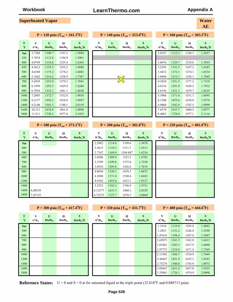
Workbook LearnThermo.com Appendix A
Superheated Vapor WaterAE
ToF
Vft3/lbm
UBtu/lbm
HBtu/lbm
SBtu/lbm
oR
Vft3/lbm
UBtu/lbm
HBtu/lbm
SBtu/lbm
oR
Vft3/lbm
UBtu/lbm
HBtu/lbm
SBtu/lbm
oR
Sat 3.7288 1108.7 1191.5 1.5894 2.8347 1112.3 1196.3 1.5657350 3.7834 1112.8 1196.9 1.5961400 4.0799 1134.8 1225.4 1.6303 3.0076 1129.7 1218.8 1.5925450 4.3612 1155.3 1252.2 1.6606 3.2293 1151.5 1247.2 1.6245500 4.6340 1175.2 1278.2 1.6883 3.4412 1172.1 1274.1 1.6534600 5.1642 1214.2 1328.9 1.7387 3.8484 1212.1 1326.1 1.7049700 5.6829 1253.0 1379.3 1.7841 4.2434 1251.5 1377.2 1.7510800 6.1950 1292.3 1429.9 1.8260 4.6316 1291.0 1428.2 1.7932900 6.7030 1332.1 1481.1 1.8650 5.0156 1331.1 1479.7 1.8325
1000 7.2083 1372.7 1532.8 1.9018 5.3968 1371.8 1531.7 1.86951200 8.2137 1456.2 1638.8 1.9697 6.1540 1455.6 1638.0 1.93761400 9.2148 1543.3 1748.1 2.0319 6.9069 1542.9 1747.5 1.99991600 10.213 1634.0 1861.0 2.0896 7.6574 1633.7 1860.5 2.05771800 11.211 1728.3 1977.4 2.1435 8.4063 1728.0 1977.1 2.1116
ToF
Vft3/lbm
UBtu/lbm
HBtu/lbm
SBtu/lbm
oR
Vft3/lbm
UBtu/lbm
HBtu/lbm
SBtu/lbm
oR
Vft3/lbm
UBtu/lbm
HBtu/lbm
SBtu/lbm
oR
Sat 2.2882 1114.8 1199.6 1.5470400 2.3615 1124.2 1211.7 1.5613500 2.7247 1169.0 1269.887 1.6254600 3.0586 1209.9 1323.2 1.6782700 3.3795 1249.8 1375.0 1.7250800 3.6934 1289.8 1426.6 1.7676900 4.0030 1330.1 1478.3 1.8072
1000 4.3098 1371.0 1530.6 1.84431200 4.9182 1455.0 1637.1 1.91271400 5.5222 1542.4 1746.9 1.97511600 6.80539 6.12377 1633.3 1860.1 2.03291800 7.47155 6.72375 1727.7 1976.7 2.0869
ToF
Vft3/lbm
UBtu/lbm
HBtu/lbm
SBtu/lbm
oR
Vft3/lbm
UBtu/lbm
HBtu/lbm
SBtu/lbm
oR
Vft3/lbm
UBtu/lbm
HBtu/lbm
SBtu/lbm
oR
Sat 1.1616 1119.8 1205.8 1.4862500 1.2851 1151.2 1246.4 1.5298600 1.47653 1198.4 1307.8 1.5907700 1.65073 1241.5 1363.8 1.6413800 1.81661 1283.3 1417.9 1.6860900 1.97772 1324.9 1471.4 1.7269
1000 2.13582 1366.7 1524.9 1.76491200 2.44647 1451.9 1633.1 1.83431400 2.75274 1540.0 1743.9 1.89731600 3.05647 1631.4 1857.8 1.95551800 3.35861 1726.1 1974.9 2.0098
Reference States: U = 0 and S = 0 at for saturated liquid at the triple point (32.018oF and 0.088713 psia).
P = 300 psia (Tsat = 417.4oF) P = 350 psia (Tsat = 431.7oF) P = 400 psia (Tsat = 444.6oF)
Page 539
P = 160 psia (Tsat = 363.5oF)
P = 180 psia (Tsat = 373.1oF) P = 200 psia (Tsat = 381.8oF) P = 250 psia (Tsat = 401.0oF)
P = 120 psia (Tsat = 341.3oF) P = 140 psia (Tsat = 353.0oF)
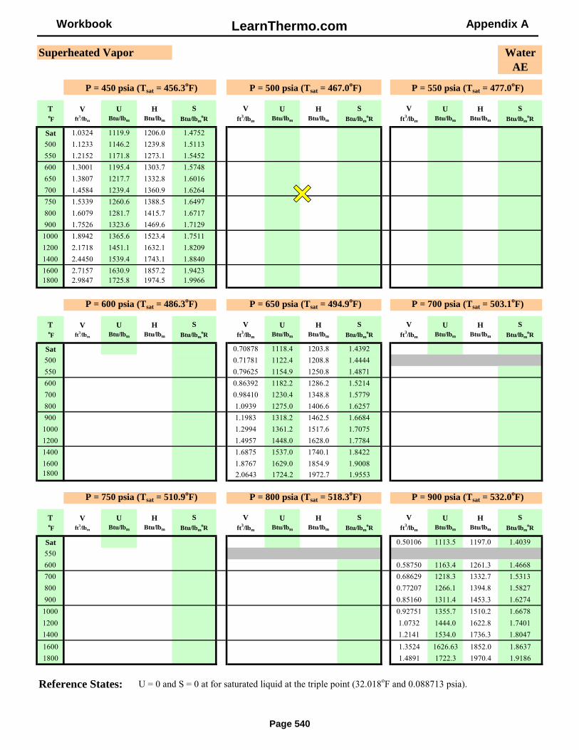
Workbook LearnThermo.com Appendix A
Superheated Vapor WaterAE
ToF
Vft3/lbm
UBtu/lbm
HBtu/lbm
SBtu/lbm
oR
Vft3/lbm
UBtu/lbm
HBtu/lbm
SBtu/lbm
oR
Vft3/lbm
UBtu/lbm
HBtu/lbm
SBtu/lbm
oR
Sat 1.0324 1119.9 1206.0 1.4752500 1.1233 1146.2 1239.8 1.5113550 1.2152 1171.8 1273.1 1.5452600 1.3001 1195.4 1303.7 1.5748650 1.3807 1217.7 1332.8 1.6016700 1.4584 1239.4 1360.9 1.6264750 1.5339 1260.6 1388.5 1.6497800 1.6079 1281.7 1415.7 1.6717900 1.7526 1323.6 1469.6 1.7129
1000 1.8942 1365.6 1523.4 1.75111200 2.1718 1451.1 1632.1 1.82091400 2.4450 1539.4 1743.1 1.88401600 2.7157 1630.9 1857.2 1.94231800 2.9847 1725.8 1974.5 1.9966
ToF
Vft3/lbm
UBtu/lbm
HBtu/lbm
SBtu/lbm
oR
Vft3/lbm
UBtu/lbm
HBtu/lbm
SBtu/lbm
oR
Vft3/lbm
UBtu/lbm
HBtu/lbm
SBtu/lbm
oR
Sat 0.70878 1118.4 1203.8 1.4392500 0.71781 1122.4 1208.8 1.4444550 0.79625 1154.9 1250.8 1.4871600 0.86392 1182.2 1286.2 1.5214700 0.98410 1230.4 1348.8 1.5779800 1.0939 1275.0 1406.6 1.6257900 1.1983 1318.2 1462.5 1.6684
1000 1.2994 1361.2 1517.6 1.70751200 1.4957 1448.0 1628.0 1.77841400 1.6875 1537.0 1740.1 1.84221600 1.8767 1629.0 1854.9 1.90081800 2.0643 1724.2 1972.7 1.9553
ToF
Vft3/lbm
UBtu/lbm
HBtu/lbm
SBtu/lbm
oR
Vft3/lbm
UBtu/lbm
HBtu/lbm
SBtu/lbm
oR
Vft3/lbm
UBtu/lbm
HBtu/lbm
SBtu/lbm
oR
Sat 0.50106 1113.5 1197.0 1.4039550600 0.58750 1163.4 1261.3 1.4668700 0.68629 1218.3 1332.7 1.5313800 0.77207 1266.1 1394.8 1.5827900 0.85160 1311.4 1453.3 1.6274
1000 0.92751 1355.7 1510.2 1.66781200 1.0732 1444.0 1622.8 1.74011400 1.2141 1534.0 1736.3 1.80471600 1.3524 1626.63 1852.0 1.86371800 1.4891 1722.3 1970.4 1.9186
Reference States: U = 0 and S = 0 at for saturated liquid at the triple point (32.018oF and 0.088713 psia).
P = 750 psia (Tsat = 510.9oF) P = 800 psia (Tsat = 518.3oF) P = 900 psia (Tsat = 532.0oF)
Page 540
P = 600 psia (Tsat = 486.3oF)
P = 450 psia (Tsat = 456.3oF)
P = 700 psia (Tsat = 503.1oF)
P = 550 psia (Tsat = 477.0oF) P = 500 psia (Tsat = 467.0oF)
P = 650 psia (Tsat = 494.9oF)

Workbook LearnThermo.com Appendix A
Superheated Vapor WaterAE
ToF
Vft3/lbm
UBtu/lbm
HBtu/lbm
SBtu/lbm
oR
Vft3/lbm
UBtu/lbm
HBtu/lbm
SBtu/lbm
oR
Vft3/lbm
UBtu/lbm
HBtu/lbm
SBtu/lbm
oR
Sat 0.18813 1067.5 1137.2 1.2872600650 0.20586 1092.1 1168.4 1.3155700 0.24894 1148.4 1240.6 1.3793750 0.28074 1188.2 1292.1 1.4228800 0.30763 1221.3 1335.2 1.4577900 0.35390 1278.3 1409.4 1.5145
1000 0.39479 1329.6 1475.8 1.56161100 0.43266 1378.4 1538.6 1.60321200 0.46864 1426.0 1599.6 1.64111300 0.50332 1473.3 1659.7 1.67631400 0.53708 1520.5 1719.4 1.70931600 0.60269 1616.0 1839.3 1.77051800 0.66660 1713.7 1960.6 1.8267
ToF
Vft3/lbm
UBtu/lbm
HBtu/lbm
SBtu/lbm
oR
Vft3/lbm
UBtu/lbm
HBtu/lbm
SBtu/lbm
oR
Vft3/lbm
UBtu/lbm
HBtu/lbm
SBtu/lbm
oR
Sat 0.08466 970.58 1017.6 1.1597700 0.09837 1006.0 1060.6 1.1969750 0.14840 1114.8 1197.2 1.3127800 0.17601 1168.3 1266.1 1.3685850 0.19771 1209.0 1318.8 1.4096900 0.21639 1243.6 1363.8 1.4433950 0.23321 1274.7 1404.3 1.4726
1000 0.24876 1303.7 1441.9 1.49881200 0.30367 1409.0 1577.7 1.58611400 0.35249 1508.0 1703.8 1.65791600 0.39830 1606.3 1827.6 1.72111800 0.44236 1705.8 1951.6 1.7785
ToF
Vft3/lbm
UBtu/lbm
HBtu/lbm
SBtu/lbm
oR
Vft3/lbm
UBtu/lbm
HBtu/lbm
SBtu/lbm
oR
Vft3/lbm
UBtu/lbm
HBtu/lbm
SBtu/lbm
oR
Sat
700 0.028713 742.81 764.08 0.93536750 0.063703 962.70 1009.9 1.1417800 0.10520 1095.0 1172.9 1.2743850 0.12848 1157.4 1252.6 1.3364900 0.14647 1203.3 1311.8 1.3808
1000 0.17538 1275.4 1405.3 1.44731200 0.22121 1391.3 1555.1 1.54371400 0.26028 1495.3 1688.1 1.61931600 0.29620 1596.5 1815.9 1.68461800 0.33033 1698.0 1942.6 1.7434
Reference States: U = 0 and S = 0 at for saturated liquid at the triple point (32.018oF and 0.088713 psia).
P = 2000 psia (Tsat = 635.9oF) P = 1000 psia (Tsat = 544.7oF) P = 1500 psia (Tsat = 596.3oF)
P = 4000 psia P = 5000 psia P = 6000 psia
Page 541
S u p e r c r i t i c a l
P = 2500 psia (Tsat = 668.2oF) P = 3000 psia (Tsat = 695.4oF) P = 3500 psia

Workbook LearnThermo.com Appendix A .
Subcooled Liquid WaterAE
ToF
lbm/ft3
Vft3/lbm
UBtu/lbm
HBtu/lbm
SBtu/lbm
oR
lbm/ft3
Vft3/lbm
UBtu/lbm
HBtu/lbm
SBtu/lbm
oR
32.02 62.632 0.015966 0.051537 3.0081 9.4391E-0550 62.611 0.015972 18.002 20.959 0.035953
100 62.179 0.016083 67.738 70.716 0.12908150 61.380 0.016292 117.50 120.51 0.21430200 60.315 0.016580 167.42 170.49 0.29309250 59.028 0.016941 217.66 220.80 0.36659300 57.536 0.017380 268.42 271.64 0.43581350 55.835 0.017910 319.98 323.30 0.50167400 53.903 0.018552 372.73 376.16 0.56501450 51.689 0.019347 427.22 430.80 0.62678500 49.097 0.020368 484.35 488.12 0.68811
Sat 46.297 0.021600 539.02 543.019 0.74400
ToF
lbm/ft3
Vft3/lbm
UBtu/lbm
HBtu/lbm
SBtu/lbm
oR
lbm/ft3
Vft3/lbm
UBtu/lbm
HBtu/lbm
SBtu/lbm
oR
32.02 62.846 0.015912 0.090413 5.9833 1.4281E-04 63.056 0.015859 0.11927 8.9292 1.5155E-0450 62.812 0.015921 17.922 23.819 0.03577 63.010 0.015870 17.839 26.656 0.03556
100 62.365 0.016035 67.407 73.345 0.12847 62.547 0.015988 67.083 75.964 0.12785150 61.564 0.016243 116.95 122.96 0.21338 61.746 0.016195 116.41 125.41 0.21247200 60.508 0.016527 166.65 172.77 0.29190 60.698 0.016475 165.90 175.05 0.29073250 59.237 0.016881 216.64 222.89 0.36513 59.442 0.016823 215.65 225.00 0.36370300350400450500550600640680Sat
U = 0 and S = 0 at for saturated liquid at the triple point (32.018oF and 0.088713 psia).
P = 500 psia (467.0oF) P = 1000 psia (544.7oF)
P = 3000 psia (695.4oF)
Reference States:
Page 542
P = 2000 psia (635.9oF)
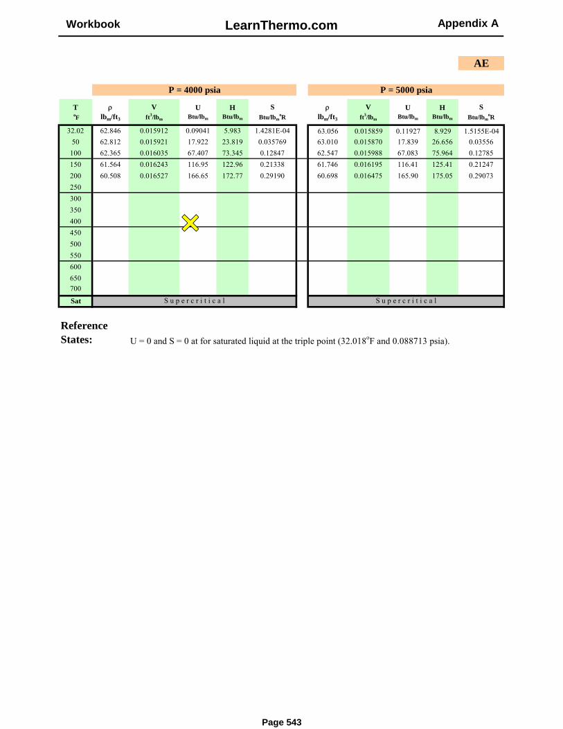
Workbook LearnThermo.com Appendix A .
AE
ToF
lbm/ft3
Vft3/lbm
UBtu/lbm
HBtu/lbm
SBtu/lbm
oR
lbm/ft3
Vft3/lbm
UBtu/lbm
HBtu/lbm
SBtu/lbm
oR
32.02 62.846 0.015912 0.09041 5.983 1.4281E-04 63.056 0.015859 0.11927 8.929 1.5155E-0450 62.812 0.015921 17.922 23.819 0.035769 63.010 0.015870 17.839 26.656 0.03556
100 62.365 0.016035 67.407 73.345 0.12847 62.547 0.015988 67.083 75.964 0.12785150 61.564 0.016243 116.95 122.96 0.21338 61.746 0.016195 116.41 125.41 0.21247200 60.508 0.016527 166.65 172.77 0.29190 60.698 0.016475 165.90 175.05 0.29073250300350400450500550600650700
Sat
U = 0 and S = 0 at for saturated liquid at the triple point (32.018oF and 0.088713 psia).
Page 543
Reference States:
P = 4000 psia P = 5000 psia
S u p e r c r i t i c a l S u p e r c r i t i c a l

Workbook LearnThermo.com Appendix B
Saturation Temperature Table NH3
SI
Sat. Liq Sat. Vap Sat. Liq Sat. Vap Sat. Liq Sat. Vap Sat. Liq Sat. Vap
-60 21.893 0.0014013 4.7057 -87.262 1251.5 -87.232 1354.6 -0.39078 6.3735-55 30.145 0.0014126 3.4895 -65.679 1258.2 -65.637 1363.4 -0.29069 6.2600-50 40.836 0.0014243 2.6277 -43.956 1264.7 -43.897 1372.0 -0.19223 6.1529-45 54.489 0.0014364 -22.096 1380.4 6.0517-40 71.692 0.0014490 -0.10388 1388.6 5.9558-35 93.098 0.0014619 22.015 1396.5 5.8648-30 119.43 0.0014753 44.257 1404.1 5.7784-25 151.47 0.0014891 66.617 1411.5 5.6960-20 190.08 0.0015035 89.095 1418.5 5.6174-15 236.17 0.0015183 111.69 1425.2 5.5422-10 290.71 0.0015336 134.39 1431.5 5.4701-5 354.76 0.0015495 157.22 1437.5 5.40090 429.38 0.0015660 180.16 1443.1 5.33435 515.75 0.0015831 203.22 1448.2 5.2700
10 615.05 0.0016009 226.41 1452.9 5.207915 728.52 0.0016195 249.74 1457.2 5.147720 857.48 0.0016388 273.21 1461.0 5.089125 1003.2 0.0016590 296.83 1464.3 5.032130 1167.2 0.0016802 320.63 1467.0 4.976435 1350.8 0.0017024 344.60 1469.2 4.921840 1555.4 0.0017258 368.78 1470.7 4.868245 1782.7 0.0017505 393.18 1471.7 4.815350 2034.0 0.0017766 417.84 1471.9 4.763055 2311.1 0.0018044 442.76 1471.4 4.711060 2615.6 0.0018340 468.00 1470.1 4.659165 2949.1 0.0018658 493.59 1467.9 4.607170 3313.5 0.0019000 519.58 1464.8 4.554875 3710.5 0.0019371 546.02 1460.6 4.501780 4142.0 0.0019776 572.98 1455.1 4.447785 4610.0 0.0020221 600.55 1448.4 4.392190 5116.7 0.0020714 628.84 1440.0 4.334695 5664.3 0.0021269 657.97 1429.8 4.2744
100 6255.3 0.0021899 688.13 1417.5 4.2107105 6892.3 0.0022630 719.58 1402.4 4.1424110 7578.3 0.0023496 752.71 1383.9 4.0675115 8317.0 0.0024559 788.14 1360.8 3.9835120 9112.5 0.0025941 827.11 1331.1 3.8852
132.25 11333 0.0044444 1049.7 1100.1 3.2674
Reference States: H = 0 kJ/kg for saturated liquid at-40°C.S = 0 kJ/kg-K for saturated liquid at -40 °C.
S (kJ/kg*K)V (m3/kg) U (kJ/kg) H (kJ/kg)
Page 544
Temp.
(oC)Pressure
(kPa)

Workbook LearnThermo.com Appendix B
Saturation Pressure Table NH3
SI
Sat. Liq Sat. Vap Sat. Liq Sat. Vap Sat. Liq Sat. Vap Sat. Liq Sat. Vap
10 -71.22 0.0013773 9.8000 -135.17 1236.1 -135.16 1334.1 -0.62165 6.654530 -55.08 0.0014124 3.5053 -66.014 1258.1 -65.972 1363.3 -0.29223 6.261750 -46.52 0.0014327 2.1749 -28.743 1269.1 -28.671 1377.9 -0.12459 6.0818
100 -33.59 0.0014656 1284.9 28.429 5.8400200 -18.85 0.0015068 1301.1 94.591 5.5998250 -13.65 0.0015224 1306.4 118.18 5.5225500 4.14 0.0015801 1322.2 200.03 5.2809750 15.88 0.0016228 1330.6 255.06 5.1373
1000 24.90 0.0016586 1335.7 297.99 5.03331250 32.32 0.0016904 1339.0 333.86 4.95091500 38.70 0.0017196 1341.1 365.04 4.88211750 44.31 0.0017470 1342.4 392.87 4.82252000 49.35 0.0017732 1343.0 418.17 4.76972250 53.94 0.0017984 1343.1 441.49 4.72202500 58.16 0.0018229 1342.7 463.21 4.67822750 62.07 0.0018469 1342.0 483.62 4.63763000 65.72 0.0018706 1341.0 502.94 4.59963250 69.16 0.0018941 1339.7 521.33 4.56363500 72.40 0.0019175 1338.1 538.93 4.52943750 75.48 0.0019408 1336.2 555.84 4.49674000 78.40 0.0019642 1334.2 572.15 4.46514250 81.19 0.0019878 1331.9 587.93 4.43464500 83.86 0.0020115 1329.4 603.26 4.40494750 86.42 0.0020356 1326.7 618.18 4.37605000 88.88 0.0020599 1323.8 632.75 4.34775250 91.25 0.0020847 1320.7 647.00 4.31985500 93.54 0.0021100 1317.3 660.97 4.29235750 95.75 0.0021358 1313.8 674.70 4.26516000 97.89 0.0021622 1310.0 688.22 4.23826250 99.96 0.0021894 1306.1 701.55 4.21136500 101.97 0.0022173 1301.9 714.74 4.18456750 103.92 0.0022461 1297.4 727.80 4.15777000 105.81 0.0022760 1292.8 740.76 4.13077250 107.65 0.0023069 1287.8 753.65 4.10367500 109.45 0.0023392 1282.6 766.49 4.07627750 111.20 0.0023729 1277.0 779.33 4.04848000 112.90 0.0024083 1271.2 792.18 4.02018500 116.18 0.0024851 1258.3 818.10 3.96179000 119.32 0.0025725 1243.6 844.64 3.89989500 122.31 0.0026755 1226.5 872.39 3.8325
11333 132.25 0.0044444 1049.7 1100.1 3.2674
Reference States: H = 0 kJ/kg for saturated liquid at-40°C.S = 0 kJ/kg-K for saturated liquid at -40 °C.
S (kJ/kg*K)
Page 545
Pressure(kPa)
Temp.
(oC)V (m3/kg) U (kJ/kg) H (kJ/kg)

Workbook LearnThermo.com Appendix B
Superheated Vapor NH3
SI
Temp.
(oC)
V
(m3/kg)
U(kJ/kg)
H(kJ/kg)
S(kJ/kg*K)
V
(m3/kg)
U(kJ/kg)
H(kJ/kg)
S(kJ/kg*K)
V
(m3/kg)
U(kJ/kg)
H(kJ/kg)
S(kJ/kg*K)
Sat 1.1381 1284.9 1398.7 5.8400-40-30 1.1573 1291.2 1406.9 5.8739-20 1.2102 1308.3 1429.4 5.9645-10 1.2622 1325.2 1451.5 6.05020 1.3136 1342.0 1473.3 6.1317
10 1.3646 1358.6 1495.1 6.209820 1.4153 1375.2 1516.7 6.285030 1.4656 1391.8 1538.3 6.357540 1.5158 1408.4 1560.0 6.427850 1.5657 1425.2 1581.7 6.496160 1.6155 1442.0 1603.5 6.562670 1.6652 1458.9 1625.4 6.6274
Temp.
(oC)
V
(m3/kg)
U(kJ/kg)
H(kJ/kg)
S(kJ/kg*K)
V
(m3/kg)
U(kJ/kg)
H(kJ/kg)
S(kJ/kg*K)
V
(m3/kg)
U(kJ/kg)
H(kJ/kg)
S(kJ/kg*K)
Sat 0.48216 1306.4 1426.9 5.5225 0.16980 1330.6 1457.9 5.13730 0.51293 1331.9 1460.2 5.6473
25 0.56685 1376.5 1518.2 5.8507 0.17770 1350.7 1484.0 5.226150 0.61898 1420.0 1574.7 6.0327 0.19781 1401.6 1550.0 5.438875 0.67012 1463.4 1630.9 6.2002 0.21661 1449.4 1611.9 5.6233
100 0.72063 1507.3 1687.5 6.3570 0.23469 1496.1 1672.2 5.7906125 0.77075 1552.0 1744.7 6.5054 0.25231 1542.8 1732.0 5.9459150 0.82058 1597.7 1802.8 6.6470 0.26963 1589.9 1792.1 6.0923175 0.87022 1644.4 1862.0 6.7829 0.28673 1637.8 1852.8 6.2317200 0.91971 1692.4 1922.3 6.9139 0.30369 1686.6 1914.4 6.3653225 0.96909 1741.6 1983.9 7.0407 0.32053 1736.5 1976.9 6.4941250 1.0184 1792.2 2046.8 7.1639 0.33728 1787.7 2040.6 6.6188275 1.0676 1844.1 2111.0 7.2838 0.35395 1840.0 2105.5 6.7400300 1.1168 1897.4 2176.6 7.4008 0.37058 1893.7 2171.6 6.8580
Reference States: H = 0 kJ/kg for saturated liquid at-40°C.S = 0 kJ/kg-K for saturated liquid at -40 °C.
P = 100 kPa (-33.59°C)
P = 250 kPa (-13.65°C) P = 500 kPa (4.14°C) P = 750 kPa (15.88°C)
Page 546
P = 50 kPa (-46.52°C) P = 200 kPa (-18.85°C)

Workbook LearnThermo.com Appendix B
Superheated Vapor NH3
SI
Temp.
(oC)
V
(m3/kg)
U(kJ/kg)
H(kJ/kg)
S(kJ/kg*K)
V
(m3/kg)
U(kJ/kg)
H(kJ/kg)
S(kJ/kg*K)
V
(m3/kg)
U(kJ/kg)
H(kJ/kg)
S(kJ/kg*K)
Sat 0.064453 1343.0 1471.9 4.76972550 0.064729 1344.9 1474.4 4.777375 0.074231 1409.8 1558.3 5.0277
100 0.082479 1465.9 1630.9 5.2293125 0.090095 1518.6 1698.7 5.4054150 0.097332 1569.8 1764.5 5.5654175 0.10432 1620.7 1829.3 5.7143200 0.11114 1671.8 1894.1 5.8550225 0.11782 1723.5 1959.2 5.9891250 0.12441 1776.1 2024.9 6.1178275 0.13093 1829.7 2091.5 6.2422300 0.13739 1884.4 2159.1 6.3628325 0.14380 1940.3 2227.8 6.4801
Temp.
(oC)
V
(m3/kg)
U(kJ/kg)
H(kJ/kg)
S(kJ/kg*K)
V
(m3/kg)
U(kJ/kg)
H(kJ/kg)
S(kJ/kg*K)
V
(m3/kg)
U(kJ/kg)
H(kJ/kg)
S(kJ/kg*K)
Sat 0.013810 1282.6 1386.1 4.0762100125 0.017196 1370.4 1499.3 4.3667150 0.020803 1461.2 1617.2 4.6543175 0.023672 1533.9 1711.5 4.8709200 0.026196 1599.4 1795.9 5.0543225 0.028513 1661.6 1875.4 5.2181250 0.030692 1722.0 1952.2 5.3686275 0.032773 1781.9 2027.7 5.5094300 0.034781 1841.6 2102.5 5.6429325 0.036731 1901.7 2177.2 5.7704350 0.038637 1962.4 2252.1 5.8932375 0.040506 2023.8 2327.6 6.0119400 0.042346 2086.2 2403.8 6.1272425 0.044161 2149.5 2480.8 6.2395
Reference States: H = 0 kJ/kg for saturated liquid at-40°C.S = 0 kJ/kg-K for saturated liquid at -40 °C.
Page 547
P = 1000 kPa (24.9°C) P = 1500 kPa (38.7°C) P = 2000 kPa (49.35°C)
P = 5000 kPa (88.88°C) P = 7500 kPa (109.45°C) P = 10000 kPa (125.17°C)

Workbook LearnThermo.com Appendix B
Subcooled Liquid NH3
SI
Temp.
(oC)
V
(m3/kg)
U(kJ/kg)
H(kJ/kg)
S(kJ/kg*K)
V
(m3/kg)
U(kJ/kg)
H(kJ/kg)
S(kJ/kg*K)
V
(m3/kg)
U(kJ/kg)
H(kJ/kg)
S(kJ/kg*K)
Sat 0.0017732 414.62 418.17 1.502340 0.0017242 368.10 371.55 1.355630 0.0016778 319.52 322.87 1.197720 0.0016361 271.87 275.15 1.037610 0.0015981 224.98 228.18 0.874580 0.0015633 178.72 181.84 0.70798
-10 0.0015311 132.99 136.05 0.53721-20 0.0015011 87.77 90.77 0.36177-30 0.0014732 43.018 45.964 0.18120-40-50-60
0.0014471 -1.2430 1.6512 -0.00489400.0014227 -44.991 -42.146 -0.196880.0013998 -88.194 -85.395 -0.39516
Temp.
(oC)
V
(m3/kg)
U(kJ/kg)
H(kJ/kg)
S(kJ/kg*K)
V
(m3/kg)
U(kJ/kg)
H(kJ/kg)
S(kJ/kg*K)
V
(m3/kg)
U(kJ/kg)
H(kJ/kg)
S(kJ/kg*K)
Sat 0.0023392 748.95 766.49 2.4566110110100 0.0021621 681.11 697.33 2.273690 0.0020388 619.34 634.63 2.103380 0.0019462 562.76 577.35 1.943470 0.0018715 509.36 523.40 1.788560 0.0018087 458.14 471.71 1.635650 0.0017543 408.50 421.65 1.483140 0.0017061 360.04 372.84 1.329630 0.0016629 312.51 324.98 1.174320 0.0016236 265.71 277.88 1.016310 0.0015876 219.51 231.42 0.855090 0.0015542 173.84 185.49 0.68996
-10 0.0015233 128.62 140.04 0.52045-20 0.0014943 83.838 95.046 0.34612-30 0.0014672 39.488 50.492 0.16656-40 0.0014418 -4.4130 6.4009 -0.018597-50 0.0014181 -47.831 -37.196 -0.20971-60 0.0013958 -90.728 -80.260 -0.40714
Reference States: H = 0 kJ/kg for saturated liquid at-40°C.S = 0 kJ/kg-K for saturated liquid at -40 °C.
Page 548
P = 1 MPa (24.9°C) P = 2000 kPa (49.35°C)P = 1500 kPa (38.7°C)
P = 5000 kPa (88.88°C) P = 7500 kPa (109.45°C) P = 10000 kPa (125.17°C)

Workbook LearnThermo.com Appendix B
Saturation Temperature Table NH3
AE
Sat. Liq Sat. Vap Sat. Liq Sat. Vap Sat. Liq Sat. Vap Sat. Liq Sat. Vap
-100 1.2374 0.021994 182.19 -61.999 530.52 -61.994 572.26 -0.15922 1.6042-95 1.5234 0.022085 149.92 -56.940 532.19 -56.934 574.48 -0.14525 1.5862-90 1.8637 0.022177 124.12 -51.862 533.86 -51.854 576.69 -0.13142 1.5689-85 2.2661 0.022272 103.35 -46.765 535.50 -46.755 578.87 -0.11773 1.5521-80 2.7394 0.022368 86.546 -41.648 537.13 -41.637 581.03 -0.10416 1.5359-75 3.2930 0.022467 72.857 -36.512 538.75 -36.499 583.17 -0.090721 1.5202-70 3.9374 0.022567 540.34 -31.341 1.5050-65 4.6837 0.022669 541.92 -26.165 1.4904-60 5.5439 0.022773 543.47 -20.969 1.4761-55 6.5312 0.022879 545.01 -15.754 1.4624-50 7.6592 0.022988 546.52 -10.521 1.4490-45 8.9429 0.023098 548.01 -5.2695 1.4360-40 10.398 0.023210 549.48 0 1.4235-35 12.041 0.023324 550.92 5.2872 1.4113-30 13.890 0.023441 552.34 10.592 1.3994-25 15.962 0.023560 553.73 15.914 1.3878-20 18.279 0.023681 555.09 21.253 1.3766-15 20.859 0.023804 556.42 26.609 1.3657-10 23.723 0.023929 557.73 31.982 1.3550-5 26.895 0.024057 559.00 37.372 1.34460 30.397 0.024187 560.24 42.779 1.33455 34.253 0.024320 561.45 48.203 1.3246
10 38.487 0.024456 562.63 53.644 1.315015 43.126 0.024594 563.77 59.103 1.305520 48.194 0.024735 564.88 64.579 1.296325 53.720 0.024879 565.95 70.072 1.287330 59.731 0.025025 566.98 75.585 1.278435 66.255 0.025175 567.97 81.116 1.269840 73.322 0.025328 568.93 86.666 1.261345 80.962 0.025484 569.84 92.237 1.252950 89.205 0.025644 570.72 97.828 1.244755 98.083 0.025808 571.55 103.44 1.236760 107.63 0.025975 572.33 109.08 1.228765 117.87 0.026146 573.07 114.73 1.221070 128.85 0.026322 573.77 120.42 1.213375 140.59 0.026502 574.41 126.13 1.205780 153.13 0.026686 575.01 131.86 1.198285 166.51 0.026876 575.55 137.62 1.190990 180.76 0.027070 576.04 143.42 1.1836
100 212.01 0.027476 576.86 155.10 1.1692120 286.60 0.028364 577.76 178.90 1.1411140 379.36 0.029379 577.54 203.40 1.1136160 492.95 0.030563 575.95 228.83 1.0858180 630.24 0.031986 572.60 255.47 1.0572200 794.38 0.033761 566.86 283.81 1.0265220 989.03 0.036110 557.63 314.65 0.99193240 1218.7 0.039556 542.46 349.77 0.94966
270.05 1643.7 0.071193 451.57 473.25 0.78093
Reference States: H = 0 Btu/lbm for saturated liquid at -40°F.S = 0 Btu/lbm°R for saturated liquid at -40°F.
Temp.
(oF)Pressure
(psia)
Page 549
S (Btu/lbmoR)V (ft3/lbm) U (Btu/lbm) H (Btu/lbm)

Workbook LearnThermo.com Appendix B
Saturation Pressure Table NH3
AE
Sat. Liq Sat. Vap Sat. Liq Sat. Vap Sat. Liq Sat. Vap Sat. Liq Sat. Vap
1 -104.96 0.021906 222.48 -67.002 528.84 -66.998 570.04 -0.17323 1.62275 -63.08 0.022709 49.310 -24.192 542.52 -24.171 588.17 -0.059178 1.4848
10 -41.31 0.023181 25.805 -1.4228 549.10 -1.3799 596.88 -0.0032891 1.426715 -27.99 0.023488 18.007 12.668 552.90 12.732 601.90 0.029867 1.394720 -16.61 0.023764 13.497 24.799 556.00 24.887 605.98 0.057608 1.369130 -0.54 0.024173 9.2292 42.056 560.11 42.191 611.38 0.095871 1.335640 11.68 0.024502 563.02 55.477 1.311850 21.68 0.024783 565.24 66.424 1.293260 30.21 0.025032 567.02 75.822 1.278070 37.70 0.025257 568.49 84.109 1.265180 44.39 0.025465 569.73 91.558 1.253990 50.46 0.025659 570.79 98.347 1.2440
100 56.03 0.025842 571.71 104.60 1.2350120 66.00 0.026181 573.21 115.87 1.2194140 74.76 0.026493 574.38 125.85 1.2061160 82.61 0.026784 575.30 134.86 1.1944180 89.74 0.027060 576.02 143.12 1.1839200 96.30 0.027323 576.58 150.76 1.1745220 102.38 0.027576 577.02 157.89 1.1658240 108.05 0.027820 577.34 164.60 1.1578260 113.37 0.028057 577.58 170.94 1.1504280 118.40 0.028289 577.73 176.97 1.1434300 123.17 0.028515 577.81 182.72 1.1368350 134.11 0.029064 577.74 196.10 1.1217400 143.94 0.029597 577.35 208.33 1.1081450 152.89 0.030119 576.69 219.66 1.0957500 161.12 0.030636 575.81 230.29 1.0842550 168.76 0.031152 574.73 240.33 1.0734600 175.90 0.031670 573.45 249.89 1.0632650 182.60 0.032193 572.00 259.05 1.0533700 188.93 0.032725 570.38 267.88 1.0438750 194.92 0.033268 568.59 276.42 1.0345800 200.63 0.033824 566.64 284.73 1.0255900 211.26 0.034992 562.20 300.79 1.0077
1000 221.03 0.036254 557.02 316.34 0.99001200 238.49 0.039233 543.92 346.89 0.95331300 246.36 0.041098 535.51 362.52 0.93321400 253.75 0.043431 525.16 379.12 0.910721500 260.70 0.046709 511.50 398.09 0.883571600 267.24 0.053180 489.23 425.50 0.84322
1643.7 270.05 0.071193 451.57 473.25 0.78093
Reference States: H = 0 Btu/lbm for saturated liquid at -40°F.S = 0 Btu/lbm°R for saturated liquid at -40°F.
Pressure(psia)
Temp.
(oF)
Page 550
S (Btu/lbmoR)V (ft3/lbm) U (Btu/lbm) H (Btu/lbm)

Workbook LearnThermo.com Appendix B
Superheated Vapor NH3
AE
ToF
Vft3/lbm
UBtu/lbm
HBtu/lbm
SBtu/lbm
oR
Vft3/lbm
UBtu/lbm
HBtu/lbm
SBtu/lbm
oR
Vft3/lbm
UBtu/lbm
HBtu/lbm
SBtu/lbm
oR
Sat 25.805 549.10 596.88 1.4267-90-80-70-60-50-40 25.894 549.63 597.58 1.4284-20 27.242 557.70 608.15 1.45300 28.569 565.63 618.53 1.4761
20 29.882 573.49 628.82 1.498040 31.185 581.31 639.06 1.518960 32.480 589.13 649.27 1.538980 33.769 596.97 659.50 1.5583
100 35.054 604.84 669.76 1.5769
ToF
Vft3/lbm
UBtu/lbm
HBtu/lbm
SBtu/lbm
oR
Vft3/lbm
UBtu/lbm
HBtu/lbm
SBtu/lbm
oR
Vft3/lbm
UBtu/lbm
HBtu/lbm
SBtu/lbm
oR
Sat 13.497 556.00 605.98 1.3691-20-10 13.730 558.83 609.68 1.37740 14.078 563.06 615.20 1.3896
10 14.423 567.23 620.65 1.401320 14.764 571.36 626.04 1.412630 15.103 575.45 631.38 1.423740 15.439 579.52 636.69 1.434450 15.772 583.56 641.98 1.444960 16.104 587.60 647.24 1.455170 16.435 591.62 652.49 1.465190 17.092 599.66 662.96 1.4845
ToF
Vft3/lbm
UBtu/lbm
HBtu/lbm
SBtu/lbm
oR
Vft3/lbm
UBtu/lbm
HBtu/lbm
SBtu/lbm
oR
Vft3/lbm
UBtu/lbm
HBtu/lbm
SBtu/lbm
oR
Sat 9.2292 560.11 611.38 1.33560 9.2424 560.35 611.70 1.3363
10 9.4836 564.79 617.47 1.348720 9.7211 569.15 623.15 1.360730 9.9554 573.44 628.74 1.372240 10.187 577.67 634.26 1.383460 10.644 586.03 645.16 1.4048
100 11.540 602.51 666.62 1.4445150 12.637 623.04 693.25 1.4901200 13.721 643.82 720.04 1.5323300 15.864 686.73 774.86 1.6097400 17.990 732.03 831.97 1.6803
Reference States: H = 0 Btu/lbm for saturated liquid at -40°F.S = 0 Btu/lbm°R for saturated liquid at -40°F.
P = 30 psia (-0.54°F) P = 40 psia (11.68°F) P = 50 psia (21.68°F)
Page 551
P = 14.696 psia (-27.99°F)
P = 1 psia (-104.96°F)
P = 25 psia (-7.93°F)
P = 10 psia (-41.31°F)P = 5 psia (-63.08°F)
P = 20 psia (-16.61°F)

Workbook LearnThermo.com Appendix B
Superheated Vapor NH3
AE
ToF
Vft3/lbm
UBtu/lbm
HBtu/lbm
SBtu/lbm
oR
Vft3/lbm
UBtu/lbm
HBtu/lbm
SBtu/lbm
oR
Vft3/lbm
UBtu/lbm
HBtu/lbm
SBtu/lbm
oR
Sat 3.8834 569.14 623.07 1.259360 4.0822 578.46 635.16 1.283080 4.2843 587.88 647.38 1.3061
100 4.4800 596.98 659.20 1.3276120 4.6709 605.88 670.75 1.3479140 4.8582 614.66 682.13 1.3672160 5.0426 623.36 693.39 1.3857180 5.2249 632.03 704.60 1.4035200 5.4052 640.71 715.78 1.4207240 5.7618 658.13 738.15 1.4536280 6.1142 675.75 760.67 1.4849320 6.4635 693.66 783.42 1.5149360 6.8105 711.90 806.49 1.5437400 7.1557 730.52 829.90 1.5716
ToF
Vft3/lbm
UBtu/lbm
HBtu/lbm
SBtu/lbm
oR
Vft3/lbm
UBtu/lbm
HBtu/lbm
SBtu/lbm
oR
Vft3/lbm
UBtu/lbm
HBtu/lbm
SBtu/lbm
oR
Sat 0.99749 577.81 633.22 1.1368120140 1.0570 589.16 647.88 1.1616160 1.1217 601.41 663.73 1.1876200 1.2393 623.61 692.46 1.2325240 1.3474 644.20 719.05 1.2717280 1.4497 664.07 744.60 1.3072320 1.5482 683.64 769.64 1.3402360 1.6439 703.17 794.49 1.3712400 1.7376 722.81 819.34 1.4008440 1.8297 742.67 844.32 1.4292500 1.9658 773.00 882.21 1.4700600 2.1885 825.36 946.94 1.5342
ToF
Vft3/lbm
UBtu/lbm
HBtu/lbm
SBtu/lbm
oR
Vft3/lbm
UBtu/lbm
HBtu/lbm
SBtu/lbm
oR
Vft3/lbm
UBtu/lbm
HBtu/lbm
SBtu/lbm
oR
Sat 0.58080 575.81 629.58 1.0842150200 0.67434 605.33 667.77 1.1440250 0.77209 635.99 707.48 1.2021300 0.85835 663.52 743.00 1.2505350 0.93835 689.81 776.69 1.2934400 1.0144 715.68 809.60 1.3329450 1.0878 741.54 842.26 1.3698500 1.1593 767.64 874.97 1.4048600 1.2982 821.13 941.33 1.4706800 1.5667 935.17 1080.2 1.5905
Reference States: H = 0 Btu/lbm for saturated liquid at -40°F.S = 0 Btu/lbm°R for saturated liquid at -40°F.
P = 400 psia (143.94°F) P = 500 psia (161.12°F) P = 1000 psia (221.03°F)
Page 552
P = 200 psia (96.3°F)
P = 75 psia (41.13°F)
P = 300 psia (123.17°F)
P = 150 psia (78.78°F)P = 100 psia (56.03°F)
P = 250 psia (110.75°F)

Workbook LearnThermo.com Appendix B
Subcooled Liquid NH3
AE
ToF
lbm/ft3
Vft3/lbm
UBtu/lbm
HBtu/lbm
SBtu/lbm
oR
lbm/ft3
Vft3/lbm
UBtu/lbm
HBtu/lbm
SBtu/lbm
oR
Sat 38.697 0.025842 104.13 104.604 0.2233550 38.999 0.025642 97.371 97.85 0.2101740 39.490 0.025323 86.246 86.714 0.1881230 39.972 0.025018 75.199 75.662 0.1657720 40.443 0.024726 64.226 64.684 0.1431210 40.906 0.024446 53.323 53.776 0.120140 41.361 0.024177 42.487 42.93463 0.096808
-10 41.808 0.023919 31.716 32.159 0.073108-20 42.247 0.023670 21.011 21.449 0.049022-30 42.679 0.023431 10.371 10.804 0.024532-40 43.103 0.023200 -0.20238 0.2272 -3.7599E-04-50 43.519 0.022978 -10.706 -10.281 -0.025718-60 43.928 0.022764 -21.139 -20.717 -0.051509-70 44.329 0.022559 -31.498 -31.080 -0.077767-80 44.722 0.022360 -41.781 -41.367 -0.10451-90 45.106 0.022170 -51.987 -51.577 -0.13176
-100 45.481 0.021987 -62.117 -61.710 -0.15955
ToF
lbm/ft3
Vft3/lbm
UBtu/lbm
HBtu/lbm
SBtu/lbm
oR
lbm/ft3
Vft3/lbm
UBtu/lbm
HBtu/lbm
SBtu/lbm
oR
Sat
9080706050403020100
-10-20-30-40-50-60-70-80-90-100
P = 150 psia (78.78°F)
P = 50 psia (21.68°F) P = 100 psia (56.03°F)
P = 200 psia (96.3°F)
Page 553

Workbook LearnThermo.com Appendix B
Subcooled Liquid AmmoniaAE
ToF
lbm/ft3
Vft3/lbm
UBtu/lbm
HBtu/lbm
SBtu/lbm
oR
lbm/ft3
Vft3/lbm
UBtu/lbm
HBtu/lbm
SBtu/lbm
oR
Sat
140120100806040200
-20-40-60-80
-100
ToF
lbm/ft3
Vft3/lbm
UBtu/lbm
HBtu/lbm
SBtu/lbm
oR
lbm/ft3
Vft3/lbm
UBtu/lbm
HBtu/lbm
SBtu/lbm
oR
Sat 32.641 0.030636 227.45 230.29 0.44104220200180160 32.725 0.030557 225.98 228.81 0.43866140 34.124 0.029305 200.58 203.29 0.39680120 35.380 0.028265 176.28 178.90 0.35544100 36.535 0.027371 152.76 155.30 0.3140080 37.616 0.026585 129.81 132.27 0.2721160 38.639 0.025881 107.28 109.68 0.2294640 39.616 0.025242 85.109 87.446 0.1858320 40.555 0.024658 63.225 65.508 0.141030 41.460 0.024120 41.601 43.834 0.094874
-20 42.336 0.023621 20.225 22.412 0.047228-40 43.182 0.023158 -0.8984 1.2457 -0.0020402-60 44.000 0.022728 -21.754 -19.650 -0.053053-80 44.786 0.022329 -42.322 -40.255 -0.105940-100 45.538 0.021959 -62.591 -60.558 -0.160871
Reference States: H = 0 Btu/lbm for saturated liquid at -40°F.S = 0 Btu/lbm°R for saturated liquid at -40°F.
Page 554
P = 300 psia (123.17°F) P = 400 psia (143.94°F)
P = 500 psia (161.12°F) P = 1000 psia (221.03°F)

Workbook LearnThermo.com Appendix C
Saturation Temperature Table R-134aSI
Sat. Liq Sat. Vap Sat. Liq Sat. Vap Sat. Liq Sat. Vap Sat. Liq Sat. Vap
-100 0.55940 0.00063195 25.193 75.362 322.76 75.362 336.85 0.43540 1.9456-95 0.93899 0.00063729 15.435 81.287 325.29 81.288 339.78 0.46913 1.9201-90 1.5241 0.00064274 9.7698 87.225 327.87 87.226 342.76 0.50201 1.8972-85 2.3990 0.00064831 330.49 93.182 345.77 0.53409 1.8766-80 3.6719 0.00065401 333.15 99.161 348.83 1 1.8580-75 5.4777 0.00065985 335.85 105.17 351.91 0.59613 1.8414-70 7.9814 0.00066583 338.59 111.20 1.8264-65 11.380 0.00067197 341.35 117.26 1.8130-60 15.906 0.00067827 344.15 123.36 1.8010-55 21.828 0.00068475 346.96 129.50 1.7902-50 29.451 0.00069142 349.80 135.67 1.7806-45 39.117 0.00069828 352.65 141.89 1.7720-40 51.209 0.00070537 355.51 148.14 1.7643-35 66.144 0.00071268 358.38 154.44 1.7575-30 84.378 0.00072025 361.25 160.79 1.7515-25 106.40 0.00072809 364.12 167.19 1.7461-20 132.73 0.00073623 366.99 173.64 1.7413-15 163.94 0.00074469 369.85 180.14 1.7371-10 200.60 0.00075351 372.69 186.70 1.7334-5 243.34 0.00076271 375.51 193.32 1.73000 292.80 0.00077233 378.31 200 1.72715 349.66 0.00078243 381.08 206.75 1.7245
10 414.61 0.00079305 383.82 213.58 1.722115 488.37 0.00080425 386.52 220.48 1.720020 571.71 0.00081610 389.17 227.47 1.718025 665.38 0.00082870 391.77 234.55 1.716230 770.20 0.00084213 394.30 241.72 1.714535 886.98 0.00085653 396.76 249.01 1.712840 1016.6 0.00087204 399.13 256.41 1.711145 1159.9 0.00088885 401.40 263.94 1.709250 1317.9 0.00090719 403.55 271.62 1.707255 1491.5 0.00092737 405.55 279.47 1.705060 1681.8 0.00094979 407.38 287.50 1.702465 1889.8 0.00097500 408.99 295.76 1.699370 2116.8 0.0010038 410.33 304.28 1.695675 2364.1 0.0010372 411.32 313.13 1.690980 2633.2 0.0010773 411.83 322.39 1.685085 2925.8 0.0011272 411.67 332.22 1.677190 3244.2 0.0011936 410.45 342.93 1.666295 3591.2 0.0012942 407.23 355.25 1.6492
100 3972.4 0.0015357 397.03 373.30 1.6109101.06 4059.3 0.0019535 381.71 389.64 1.5621
Reference States: H = 200 kJ/kg for saturated liquid at 0°C.S = 1 kJ/kg-K for saturated liquid at 0°C.
S (kJ/kg*K)V (m3/kg) U (kJ/kg) H (kJ/kg)
Page 555
Temp.
(oC)Pressure
(kPa)

Workbook LearnThermo.com Appendix C
Saturation Pressure Table R-134aSI
Sat. Liq Sat. Vap Sat. Liq Sat. Vap Sat. Liq Sat. Vap Sat. Liq Sat. Vap
50 -40.45 0.00070471 0.36925 147.54 355.25 147.57 373.71 0.79317 1.7650100 -26.36 0.00072593 0.19256 165.37 363.34 165.44 382.60 0.86756 1.7475150 -17.13 0.00074104 0.13128 177.25 368.63 177.36 388.32 0.91482 1.7388200 -10.08 0.00075337 372.64 186.60 1.7334250 -4.28 0.00076406 375.91 194.27 1.7296300 0.67 0.00077366 378.68 200.90 1.7267350 5.03 0.00078249 381.10 206.79 1.7244400 8.93 0.00079073 383.24 212.11 1.7226450 12.48 0.00079852 385.16 216.99 1.7210500 15.73 0.00080595 386.91 221.50 1.7197550 18.75 0.00081308 388.51 225.72 1.7185600 21.57 0.00081998 389.99 229.68 1.7175650 24.22 0.00082667 391.36 233.43 1.7165700 26.71 0.00083320 392.64 236.99 1.7156750 29.08 0.00083959 393.84 240.39 1.7148800 31.33 0.00084585 394.96 243.65 1.7140850 33.47 0.00085202 396.02 246.77 1.7133900 35.53 0.00085811 397.01 249.78 1.7126950 37.50 0.00086412 397.95 252.69 1.7119
1000 39.39 0.00087007 398.85 255.50 1.71131100 42.97 0.00088185 400.49 260.87 1.71001200 46.31 0.00089351 401.98 265.95 1.70871300 49.46 0.00090511 403.32 270.78 1.70751400 52.42 0.00091671 404.54 275.40 1.70621500 55.23 0.00092836 405.64 279.84 1.70491600 57.91 0.00094010 406.64 284.11 1.70361700 60.46 0.00095197 407.54 288.25 1.70221800 62.90 0.00096400 408.35 292.26 1.70071900 65.23 0.00097626 409.06 296.15 1.69922000 67.48 0.00098877 409.70 299.95 1.69762200 71.73 0.00101474 410.72 307.30 1.69412400 75.69 0.00104234 411.42 314.38 1.69022600 79.41 0.00107211 411.80 321.26 1.68582800 82.90 0.00110474 411.84 328.01 1.68073000 86.20 0.00114128 411.49 334.70 1.67483200 89.33 0.00118330 410.70 341.43 1.66793400 92.30 0.00123354 409.32 348.31 1.65953600 95.12 0.00129737 407.11 355.58 1.64873800 97.80 0.00138860 403.41 363.77 1.63364000 100.34 0.00158011 395.13 375.57 1.6046
4059.3 101.06 0.0019535 381.71 389.64 1.5621
Reference States: H = 200 kJ/kg for saturated liquid at 0°C.S = 1 kJ/kg-K for saturated liquid at 0°C.
S (kJ/kg*K)
Page 556
Pressure(kPa)
Temp.
(oC)V (m3/kg) U (kJ/kg) H (kJ/kg)

Workbook LearnThermo.com Appendix C
Superheated Vapor R-134aSI
Temp.
(oC)
V
(m3/kg)
U(kJ/kg)
H(kJ/kg)
S(kJ/kg*K)
V
(m3/kg)
U(kJ/kg)
H(kJ/kg)
S(kJ/kg*K)
V
(m3/kg)
U(kJ/kg)
H(kJ/kg)
S(kJ/kg*K)
Sat 0.31123 357.27 375.94 1.7601-30 0.32149 361.93 381.22 1.7821-20 0.33608 368.74 388.91 1.8131-10 0.35049 375.70 396.73 1.84340 0.36476 382.80 404.69 1.8730
10 0.37893 390.07 412.81 1.902220 0.39303 397.50 421.08 1.931030 0.40705 405.10 429.52 1.959340 0.42102 412.86 438.12 1.987250 0.43495 420.79 446.88 2.014760 0.44884 428.88 455.81 2.041970 0.46269 437.14 464.90 2.068880 0.47652 445.56 474.15 2.095490 0.49032 454.14 483.56 2.1217
100 0.50410 462.89 493.14 2.1477
Temp.
(oC)
V
(m3/kg)
U(kJ/kg)
H(kJ/kg)
S(kJ/kg*K)
V
(m3/kg)
U(kJ/kg)
H(kJ/kg)
S(kJ/kg*K)
V
(m3/kg)
U(kJ/kg)
H(kJ/kg)
S(kJ/kg*K)
Sat 0.083906 375.30 395.44 1.7303-100 0.086170 379.43 400.11 1.7475
10 0.090262 387.13 408.79 1.778720 0.094233 394.89 417.51 1.809030 0.098118 402.75 426.30 1.838540 0.10193 410.74 435.20 1.867450 0.10570 418.86 444.22 1.895760 0.10942 427.11 453.37 1.923670 0.11310 435.51 462.65 1.951180 0.11675 444.06 472.08 1.978190 0.12038 452.75 481.64 2.0048
100 0.12398 461.59 491.35 2.0312110 0.12756 470.58 501.20 2.0573
Reference States: H = 200 kJ/kg for saturated liquid at 0°C.S = 1 kJ/kg-K for saturated liquid at 0°C.
P = 100 kPa (-26.36°C)
P = 180 kPa (-12.71°C) P = 200 kPa (-10.08°C) P = 240 kPa (-5.37°C)
Page 557
P = 60 kPa (-36.93°C) P = 140 kPa (-18.76°C)

Workbook LearnThermo.com Appendix C
Superheated Vapor R-134aSI
Temp.
(oC)
V
(m3/kg)
U(kJ/kg)
H(kJ/kg)
S(kJ/kg*K)
V
(m3/kg)
U(kJ/kg)
H(kJ/kg)
S(kJ/kg*K)
V
(m3/kg)
U(kJ/kg)
H(kJ/kg)
S(kJ/kg*K)
Sat 0.051207 383.24 403.72 1.72260
10 0.051506 384.12 404.72 1.726120 0.054214 392.32 414.01 1.758430 0.056797 400.50 423.22 1.789340 0.059293 408.73 432.45 1.819250 0.061724 417.05 441.74 1.848460 0.064104 425.47 451.11 1.877070 0.066443 434.01 460.58 1.905080 0.068748 442.67 470.17 1.932590 0.071023 451.47 479.88 1.9597
100 0.073275 460.41 489.72 1.9864110 0.075505 469.48 499.68 2.0127120 0.077717 478.69 509.78 2.0387130 0.079914 488.05 520.02 2.0645140 0.082097 497.55 530.39 2.0899
Temp.
(oC)
V
(m3/kg)
U(kJ/kg)
H(kJ/kg)
S(kJ/kg*K)
V
(m3/kg)
U(kJ/kg)
H(kJ/kg)
S(kJ/kg*K)
V
(m3/kg)
U(kJ/kg)
H(kJ/kg)
S(kJ/kg*K)
Sat 0.034300 389.99 410.57 1.71752030 0.035984 397.37 418.96 1.745540 0.037865 406.01 428.73 1.777250 0.039659 414.63 438.43 1.807760 0.041389 423.30 448.13 1.837370 0.043070 432.04 457.88 1.866180 0.044710 440.87 467.70 1.894390 0.046319 449.82 477.61 1.9220
100 0.047900 458.88 487.62 1.9492110 0.049459 468.06 497.74 1.9759120 0.050998 477.37 507.97 2.0023130 0.052520 486.82 518.33 2.0283140 0.054027 496.39 528.81 2.0540
150 0.055522 506.11 539.42 2.0794160 0.057006 515.96 550.16 2.1045
Reference States: H = 200 kJ/kg for saturated liquid at 0°C.S = 1 kJ/kg-K for saturated liquid at 0°C.
Page 558
P = 280 kPa (-1.23°C) P = 320 kPa (2.48°C) P = 400 kPa (8.93°C)
P = 500 kPa (15.73°C) P = 600 kPa (21.57°C) P = 700 kPa (26.71°C)

Workbook LearnThermo.com Appendix C
Superheated Vapor R-134aSI
Temp.
(oC)
V
(m3/kg)
U(kJ/kg)
H(kJ/kg)
S(kJ/kg*K
)
V
(m3/kg)
U(kJ/kg)
H(kJ/kg)
S(kJ/kg*K)
V
(m3/kg)
U(kJ/kg)
H(kJ/kg)
S(kJ/kg*K)
Sat 0.025625 394.96 415.46 1.714040 0.027036 402.97 424.59 1.743650 0.028547 412.00 434.84 1.775860 0.029974 420.97 444.95 1.806770 0.031340 429.96 455.03 1.836580 0.032659 438.99 465.12 1.865490 0.033942 448.10 475.25 1.8937
100 0.035193 457.30 485.45 1.9214110 0.036420 466.60 495.74 1.9486120 0.037626 476.02 506.12 1.9754130 0.038813 485.55 516.60 2.0017140 0.039985 495.21 527.20 2.0277150 0.041144 504.99 537.91 2.0533160 0.042291 514.91 548.74 2.0786170 0.043427 524.96 559.70 2.1036180 0.044554 535.14 570.78 2.1283
Temp.
(oC)
V
(m3/kg)
U(kJ/kg)
H(kJ/kg)
S(kJ/kg*K
)
V
(m3/kg)
U(kJ/kg)
H(kJ/kg)
S(kJ/kg*K)
V
(m3/kg)
U(kJ/kg)
H(kJ/kg)
S(kJ/kg*K)
Sat 0.016718 401.98 422.04 1.708750 0.017201 405.77 426.41 1.722360 0.018404 415.70 437.79 1.757070 0.019502 425.36 448.76 1.789580 0.020530 434.90 459.53 1.820490 0.021506 444.41 470.22 1.8502
100 0.022443 453.94 480.87 1.8792110 0.023348 463.53 491.54 1.9074120 0.024228 473.18 502.25 1.9350130 0.025087 482.92 513.03 1.9621140 0.025928 492.76 523.87 1.9886150 0.026753 502.70 534.81 2.0148160 0.027566 512.76 545.84 2.0405170 0.028367 522.93 556.97 2.0660
180 0.029159 533.23 568.22 2.0911190 0.029941 543.64 579.57 2.1158
Reference States: H = 200 kJ/kg for saturated liquid at 0°C.S = 1 kJ/kg-K for saturated liquid at 0°C.
Page 559
P = 800 kPa (31.33°C) P = 900 kPa (35.53°C) P = 1000 kPa (39.39°C)
P = 1200 kPa (46.31°C) P = 1400 kPa (52.42°C) P = 1600 kPa (57.91°C)

Workbook LearnThermo.com Appendix C
Subcooled Liquid R-134aSI
Temp.
(oC)
V
(m3/kg)
U(kJ/kg)
H(kJ/kg)
S(kJ/kg*K)
V
(m3/kg)
U(kJ/kg)
H(kJ/kg)
S(kJ/kg*K)
V
(m3/kg)
U(kJ/kg)
H(kJ/kg)
S(kJ/kg*K)
Sat 0.00087007 254.63 255.50 1.187635 0.00085591 248.14 249.00 1.166730 0.00084104 240.87 241.72 1.142825 0.00082731 233.73 234.56 1.119020 0.00081454 226.69 227.50 1.095215 0.00080260 219.74 220.55 1.071210 0.00079136 212.88 213.68 1.04720 0.00077069 199.39 200.16 0.99860
-10 0.00075198 186.17 186.92 0.94921-20 0.00073485 173.18 173.91 0.89881-30 0.00071903 160.39 161.11 0.84722-40 0.00070428 147.79 148.50 0.79425
Temp.
(oC)
V
(m3/kg)
U(kJ/kg)
H(kJ/kg)
S(kJ/kg*K)
V
(m3/kg)
U(kJ/kg)
H(kJ/kg)
S(kJ/kg*K)
V
(m3/kg)
U(kJ/kg)
H(kJ/kg)
S(kJ/kg*K)
Sat 0.00091671 274.12 275.40 1.24895550 0.00090646 270.32 271.59 1.237145 0.00088706 262.63 263.87 1.213140 0.00086962 255.12 256.34 1.189235 0.00085376 247.76 248.96 1.165430 0.00083919 240.53 241.71 1.141725 0.00082569 233.42 234.57 1.118020 0.00081312 226.40 227.54 1.094215 0.00080134 219.48 220.60 1.070310 0.00079024 212.64 213.75 1.04635 0.00077974 205.88 206.97 1.02220 0.00076978 199.18 200.26 0.99782-5 0.00076029 192.55 193.61 0.97327
-10 0.00075123 185.98 187.03 0.94850-15 0.00074256 179.47 180.51 0.92346-20 0.00073423 173.01 174.04 0.89815-25 0.00072622 166.60 167.62 0.87254-30 0.00071850 160.24 161.25 0.84661-40 0.00070383 147.66 148.64 0.79368
Reference States: H = 200 kJ/kg for saturated liquid at 0°C.S = 1 kJ/kg-K for saturated liquid at 0°C.
Page 560
P = 800 kPa (31.33°C) P = 1000 kPa (39.39°C)P = 900 kPa (35.53°C)
P = 1200 kPa (46.31°C) P = 1400 kPa (52.42°C) P = 1600 kPa (57.91°C)

Workbook LearnThermo.com Appendix C
Saturation Temperature Table R-134aAE
Sat. Liq Sat. Vap Sat. Liq Sat. Vap Sat. Liq Sat. Vap Sat. Liq Sat. Vap
-40 7.4272 0.011299 5.7839 63.718 152.95 63.733 160.90 0.19016 0.42169-35 8.5756 0.011364 5.0544 65.219 153.63 65.237 161.66 0.19371 0.42076-30 9.8624 0.011429 4.4330 66.725 154.32 66.746 162.41 0.19724 0.41989-25 11.299 0.011496 155.00 0.20074 0.41907-20 12.898 0.011565 155.69 0 0.41831-15 14.671 0.011635 156.38 0.20766 0.41760-10 16.632 0.011706 157.06 0.41693-5 18.794 0.011779 157.75 0.416310 21.171 0.011853 158.43 0.415725 23.777 0.011929 159.11 0.41518
10 26.628 0.012007 159.79 0.4146715 29.739 0.012086 160.47 0.4141920 33.124 0.012168 161.14 0.4137425 36.800 0.012251 161.82 0.4133232 42.468 0.012372 162.75 0.4127840 49.741 0.012515 163.81 0.4122245 54.749 0.012608 164.47 0.4119050 60.134 0.012703 165.12 0.4115955 65.913 0.012802 165.77 0.4113160 72.105 0.012903 166.41 0.4110365 78.729 0.013008 167.05 0.4107770 85.805 0.013116 167.67 0.4105275 93.351 0.013229 168.30 0.4102880 101.39 0.013345 168.91 0.4100585 109.93 0.013465 169.51 0.4098290 119.01 0.013590 170.11 0.4095995 128.65 0.013720 170.69 0.40937
100 138.85 0.013856 171.26 0.40914105 149.65 0.013998 171.82 0.40891110 161.07 0.014146 172.37 0.40867115 173.14 0.014301 172.90 0.40842120 185.86 0.014464 173.41 0.40815125 199.28 0.014636 173.91 0.40787130 213.41 0.014817 174.38 0.40757135 228.28 0.015010 174.83 0.40725140 243.92 0.015214 175.26 0.40689145 260.36 0.015432 175.66 0.40650150 277.61 0.015666 176.02 0.40606160 314.73 0.016191 176.64 0.40503170 355.53 0.016815 177.05 0.40371180 400.34 0.017588 177.19 0.40196190 588.75 0.031292 164.22 0.37335200 503.59 0.020096 175.80 0.39577
213.91 588.72 0.031292 164.22 0.37335
Reference States: H = 85.985 Btu/lbm for Saturated Liquid at 32°F.S = 0.23885 Btu/lbm-°R for Saturated Liquid at 32°F.
Page 561
Temp.
(oF)Pressure
(psia)V (ft3/lbm) U (Btu/lbm) H (Btu/lbm) S (Btu/lbm
oR)

Workbook LearnThermo.com Appendix C
Saturation Pressure Table R-134aAE
Sat. Liq Sat. Vap Sat. Liq Sat. Vap Sat. Liq Sat. Vap Sat. Liq Sat. Vap
5 -53.07 0.011135 8.3793 59.821 151.16 59.832 158.92 0.18072 0.4244110 -29.50 0.011436 4.3756 66.877 154.39 66.898 162.49 0.19759 0.4198015 -14.13 0.011647 2.9882 71.548 156.50 71.581 164.80 0.20826 0.4174820 -2.40 0.011817 158.10 75.194 166.54 0.21624 0.4160025 7.20 0.011963 159.41 78.184 0.4149530 15.40 0.012093 160.52 80.760 0.4141535 22.60 0.012211 161.49 83.040 0.4135240 29.05 0.012320 162.36 85.095 0.4130145 34.90 0.012423 163.14 86.974 0.4125750 40.27 0.012520 163.85 88.709 0.4122055 45.24 0.012612 164.50 90.326 0.4118860 49.88 0.012701 165.11 91.844 0.4116065 54.23 0.012787 165.67 93.276 0.4113570 58.34 0.012869 166.20 94.633 0.4111280 65.92 0.013028 167.16 97.162 0.4107385 69.45 0.013104 167.61 98.346 0.4105590 72.82 0.013179 168.03 99.484 0.4103995 76.05 0.013253 168.43 100.58 0.41023
100 79.16 0.013325 168.81 101.64 0.41009110 85.04 0.013466 169.52 103.66 0.40982120 90.53 0.013604 170.17 105.56 0.40957130 95.68 0.013738 170.77 107.36 0.40934140 100.55 0.013871 171.32 109.08 0.40911150 105.16 0.014002 171.84 110.72 0.40890160 109.54 0.014132 172.32 112.30 0.40869170 113.73 0.014261 172.76 113.82 0.40848180 117.73 0.014389 173.18 115.28 0.40827190 121.57 0.014517 173.57 116.70 0.40807200 125.26 0.014645 173.93 118.07 0.40786220 132.25 0.014902 174.59 120.70 0.40743240 138.77 0.015163 175.16 123.21 0.40698260 144.89 0.015428 175.65 125.61 0.40651280 150.67 0.015699 176.07 127.91 0.40600300 156.15 0.015978 176.42 130.14 0.40546320 161.35 0.016268 176.71 132.30 0.40487340 166.30 0.016570 176.93 134.41 0.40424360 171.04 0.016888 177.08 136.47 0.40355380 175.58 0.017223 177.17 138.50 0.40280400 179.93 0.017582 177.19 140.51 0.40197450 190.09 0.018614 176.88 145.47 0.39948475 194.83 0.019238 176.50 147.98 0.39793500 199.37 0.019977 175.91 150.57 0.39607
588.75 213.91 0.031292 164.22 167.63 0.37335
Reference States: H = 85.985 Btu/lbm for Saturated Liquid at 32°F.S = 0.23885 Btu/lbm-°R for Saturated Liquid at 32°F.
Page 562
Pressure(psia)
Temp.
(oF)V (ft3/lbm) U (Btu/lbm) H (Btu/lbm) S (Btu/lbm
oR)

Workbook LearnThermo.com Appendix C
Superheated Vapor R-134aAE
Temp.
(oC)
Vft3/lbm
UBtu/lbm
HBtu/lbm
SBtu/lbm
oR
Vft3/lbm
UBtu/lbm
HBtu/lbm
SBtu/lbm
oR
Vft3/lbm
UBtu/lbm
HBtu/lbm
SBtu/lbm
oR
Sat 37.834 145.20 152.20 0.43789-20 46.109 156.61 165.14 0.470220 48.229 159.78 168.72 0.47816
20 50.346 163.06 172.38 0.4859740 52.461 166.44 176.15 0.4936660 54.574 169.91 180.01 0.5012480 56.685 173.47 183.97 0.50871
100 58.796 177.13 188.02 0.51608120 60.906 180.88 192.16 0.52335140 63.015 184.73 196.40 0.53053160 65.123 188.66 200.72 0.53762180 67.231 192.68 205.13 0.54463200 69.338 196.79 209.63 0.55156220 71.445 200.99 214.22 0.55841240 73.552 205.28 218.90 0.56519
Temp.
(oC)
Vft3/lbm
UBtu/lbm
HBtu/lbm
SBtu/lbm
oR
Vft3/lbm
UBtu/lbm
HBtu/lbm
SBtu/lbm
oR
Vft3/lbm
UBtu/lbm
HBtu/lbm
SBtu/lbm
oR
Sat 1.1761 162.36 171.07 0.413010
2040 1.2126 164.41 173.39 0.4177060 1.2768 168.15 177.60 0.4259780 1.3389 171.92 181.83 0.43396
100 1.3995 175.74 186.11 0.44173120 1.4589 179.63 190.44 0.44933140 1.5173 183.59 194.83 0.45678160 1.5751 187.63 199.29 0.46410180 1.6322 191.73 203.82 0.47130200 1.6888 195.92 208.43 0.47839220 1.7449 200.18 213.11 0.48537240 1.8007 204.53 217.86 0.49227
Reference States: H = 85.985 Btu/lbm for Saturated Liquid at 32°F.S = 0.23885 Btu/lbm-°R for Saturated Liquid at 32°F.
Page 563
P = 20 psia (-2.4°F) P = 30 psia (15.4°F) P = 40 psia (29.05°F)
P = 1 psia (-97.56°F) P = 10 psia (-29.5°F) P = 14.696 psia (-14.93°F)

Workbook LearnThermo.com Appendix C
Superheated Vapor R-134aAE
Temp.
(oC)
V
(m3/kg)
U(kJ/kg)
H(kJ/kg)
S(kJ/kg*K)
V
(m3/kg)
U(kJ/kg)
H(kJ/kg)
S(kJ/kg*K)
Vft3/lbm
UBtu/lbm
HBtu/lbm
SBtu/lbm
oR
Sat 0.68214 166.20 175.04 0.4111260 0.81790 167.11 176.20 0.4160180 0.72710 170.56 179.99 0.42048
100 0.76618 174.57 184.50 0.42869120 0.80372 178.59 189.01 0.43661140 0.84013 182.66 193.55 0.44431160 0.87565 186.78 198.13 0.45183180 0.91047 190.97 202.77 0.45919200 0.94472 195.22 207.46 0.46642220 0.97849 199.54 212.22 0.47352240 1.0119 203.93 217.05 0.48051260 1.0449 208.39 221.94 0.48741280 1.0776 212.93 226.90 0.49421300 1.1101 217.54 231.93 0.50092320 1.1424 222.23 237.04 0.50756
Temp.
(oC)
V
(m3/kg)
U(kJ/kg)
H(kJ/kg)
S(kJ/kg*K)
V
(m3/kg)
U(kJ/kg)
H(kJ/kg)
S(kJ/kg*K)
Vft3/lbm
UBtu/lbm
HBtu/lbm
SBtu/lbm
oR
Sat 0.53121 168.03 176.88 0.4103980 0.54389 169.55 178.61 0.41362
100 0.57729 173.71 183.33 0.42221120 0.60874 177.85 188.00 0.43040140 0.63885 182.01 192.65 0.43830160 0.66796 186.20 197.33 0.44597180 0.69629 190.44 202.04 0.45345200 0.72400 194.74 206.80 0.46078220 0.75120 199.10 211.62 0.46797240 0.77797 203.52 216.49 0.47503260 0.80438 208.02 221.42 0.48198280 0.83049 212.58 226.42 0.48884300 0.85634 217.22 231.49 0.49559320 0.88196 221.92 236.62 0.50227
Reference States: H = 85.985 Btu/lbm for Saturated Liquid at 32°F.S = 0.23885 Btu/lbm-°R for Saturated Liquid at 32°F.
Page 564
P = 80 psia (65.92°F) P = 90 psia (72.82°F) P = 100 psia (79.16°F)
P = 50 psia (40.27°F) P = 60 psia (49.88°F) P = 70 psia (58.34°F)

Workbook LearnThermo.com Appendix C
Superheated Vapor R-134aAE
Temp.
(oC)
Vft3/lbm
UBtu/lbm
HBtu/lbm
SBtu/lbm
oR
Vft3/lbm
UBtu/lbm
HBtu/lbm
SBtu/lbm
oR
Vft3/lbm
UBtu/lbm
HBtu/lbm
SBtu/lbm
oR
Sat 0.17810 175.41 183.66 0.40675120140160 0.19527 180.33 189.37 0.41611180 0.21146 185.40 195.19 0.42535200 0.22600 190.30 200.76 0.43393220 0.23945 195.13 206.21 0.44206240 0.25213 199.93 211.60 0.44988260 0.26421 204.74 216.97 0.45744280 0.27584 209.56 222.33 0.46480300 0.28709 214.43 227.72 0.47198320 0.29803 219.33 233.13 0.47901340 0.30872 224.28 238.58 0.48591360 0.31919 229.29 244.07 0.49269380 0.32947 234.36 249.61 0.49937
Temp.
(oC)
Vft3/lbm
UBtu/lbm
HBtu/lbm
SBtu/lbm
oR
Vft3/lbm
UBtu/lbm
HBtu/lbm
SBtu/lbm
oR
Vft3/lbm
UBtu/lbm
HBtu/lbm
SBtu/lbm
oR
Sat 0.14271 176.42 184.35 0.40546 0.065644 175.91 181.98 0.39607160 0.14656 177.63 185.77 0.40776180 0.16356 183.34 192.42 0.41833 0.017125 138.11 139.70 0.33168200 0.17777 188.60 198.48 0.42765 0.066753 176.38 182.56 0.39695220 0.19044 193.67 204.25 0.43627 0.086577 185.65 193.66 0.41355240 0.20211 198.65 209.88 0.44443 0.098822 192.26 201.41 0.42479260 0.21306 203.59 215.43 0.45226 0.10876 198.19 208.26 0.43444280 0.22347 208.53 220.95 0.45982 0.11745 203.81 214.69 0.44326300 0.23346 213.48 226.45 0.46716 0.12535 209.28 220.89 0.45153320 0.24310 218.46 231.97 0.47433 0.13269 214.67 226.96 0.45942340 0.25247 223.48 237.51 0.48134 0.13960 220.02 232.95 0.46700360 0.26159 228.54 243.08 0.48822 0.14618 225.36 238.90 0.47435380 0.27052 233.66 248.69 0.49498 0.15250 230.71 244.83 0.48150400 0.27928 238.82 254.34 0.50164 0.15860 236.08 250.76 0.48848
Reference States: H = 200 kJ/kg for saturated liquid at 0°C.S = 1 kJ/kg-K for saturated liquid at 0°C.
P = 400 psia (179.93°F) P = 500 psia (199.37°F)
Page 565
P = 150 psia (105.16°F) P = 200 psia (125.26°F) P = 250 psia (141.88°F)
P = 300 psia (156.15°F)

Workbook LearnThermo.com Appendix C
Subcooled Liquid R-134aAE
Temp.
(oC)
V U H S Vft3/lbm
UBtu/lbm
HBtu/lbm
SBtu/lbm
oR
Vft3/lbm
UBtu/lbm
HBtu/lbm
SBtu/lbm
oR
Sat 0.015978 129.25 130.14 0.31743150 0.015624 126.70 127.57 0.31323120 0.014360 115.20 115.99 0.29377100 0.013754 108.06 108.83 0.2812080 0.013253 101.21 101.95 0.2686860 0.012823 94.565 95.277 0.2560840 0.012446 88.089 88.780 0.2433432 0.012307 85.539 86.223 0.2381810 0.011952 78.634 79.298 0.223770 0.011803 75.542 76.198 0.21710
-10 0.011660 72.478 73.125 0.21034-20 0.011522 69.438 70.078 0.20349-30 0.011390 66.423 67.056 0.19653-40 0.011262 63.430 64.056 0.18947-50 0.011139 60.460 61.079 0.18229
Temp.
(oC)
Vft3/lbm
UBtu/lbm
HBtu/lbm
SBtu/lbm
oR
Vft3/lbm
UBtu/lbm
HBtu/lbm
SBtu/lbm
oR
Vft3/lbm
UBtu/lbm
HBtu/lbm
SBtu/lbm
oR
Sat
350 0.057233 212.59 223.19 0.44466300 0.042185 194.14 201.95 0.41754250 0.023076 166.29 170.56 0.37474200 0.016985 142.57 145.72 0.33851180 0.015906 134.65 137.60 0.32602160 0.015084 127.17 129.96 0.31389140 0.014423 120.00 122.67 0.30193120 0.013870 113.07 115.63 0.29000100 0.013396 106.33 108.81 0.2780380 0.012980 99.760 102.163 0.2659360 0.012609 93.328 95.663 0.2536640 0.012274 87.019 89.292 0.2411532 0.012149 84.527 86.776 0.2360820 0.011969 80.819 83.04 0.228380 0.011687 74.718 76.882 0.21527
-20 0.011425 68.706 70.822 0.20180-30 0.011301 65.732 67.825 0.19490-40 0.011181 62.778 64.848 0.18789-50 0.011064 59.843 61.891 0.18076
Reference States: H = 200 kJ/kg = 85.985 Btu/lbm for Saturated Liquid at 0°C = 32°F.S = 1 kJ/kg = 0.23885 Btu/lbm-°R for Saturated Liquid at 0°C = 32°F.
P = 100 psia (79.16°F) P = 200 psia (125.26°F) P = 300 psia (156.15°F)
P = 500 psia (199.37°F) P = 1000 psia P = 5000 psia
S u p e r c r i t i c a l S u p e r c r i t i c a l
Page 566

Workbook LearnThermo.com Appendix D
Ideal Gas Property Table: AIR MW = g/mole SI
T Uo Ho So Pr Vr T Uo Ho So Pr Vr
(K) (kJ/kg) (kJ/kg) (kJ/kg-K) (K) (kJ/kg) (kJ/kg) (kJ/kg-K)
298.15 820300 840310 860320 880330 900340 920350 940360 960370 980380 1000390 1020400 1040410 1060420 1080430 1100440 1150450 1200460 1250470 1300480 1350490 1400500 1450510 1500520 1550530 1600540 1650550 1700560 1750570 1800580 1850590 1900600 1950610 2000620 2100630 2200640 2300650 2400660 2500670 2600680 2700690 2800700 2900710 3000720 3500730 4000740 4500750 5000760 5500770 6000780790800
Page 567
28.970
^ ^ ^ ^ ^^

Workbook LearnThermo.com Appendix D
Ideal Gas Property Table: CO MW = g/mole SI
T Uo Ho So Pr Vr T Uo Ho So Pr Vr
(K) (kJ/kg) (kJ/kg) (kJ/kg-K) (K) (kJ/kg) (kJ/kg) (kJ/kg-K)
298.15 820300 840310 860320 880330 900340 920350 940360 960370 980380 1000390 1020400 1040410 1060420 1080430 1100440 1150450 1200460 1250470 1300480 1350490 1400500 1450510 1500520 1550530 1600540 1650550 1700560 1750570 1800580 1850590 1900600 1950610 2000620 2100630 2200640 2300650 2400660 2500670 2600680 2700690 2800700 2900710 3000720 3500730 4000740 4500750 5000760 5500770 6000780790800
Page 568
28.013
^ ^ ^ ^ ^^

Workbook LearnThermo.com Appendix D
Ideal Gas Property Table: CO2 MW = g/mole SI
T Uo Ho So Pr Vr T Uo Ho So Pr Vr
(K) (kJ/kg) (kJ/kg) (kJ/kg-K) (K) (kJ/kg) (kJ/kg) (kJ/kg-K)
298.15 820300 840310 860320 880330 900340 920350 940360 960370 980380 1000390 1020400 1040410 1060420 1080430 1100440 1150450 1200460 1250470 1300480 1350490 1400500 1450510 1500520 1550530 1600540 1650550 1700560 1750570 1800580 1850590 1900600 1950610 2000620 2100630 2200640 2300650 2400660 2500670 2600680 2700690 2800700 2900710 3000720 3500730 4000740 4500750 5000760 5500770 6000780790800
Page 569
44.010
^ ^ ^ ^ ^^

Workbook LearnThermo.com Appendix D
Ideal Gas Property Table: H2 MW = g/mole SI
T Uo Ho So Pr Vr T Uo Ho So Pr Vr
(K) (kJ/kg) (kJ/kg) (kJ/kg-K) (K) (kJ/kg) (kJ/kg) (kJ/kg-K)
298.15 820300 840310 860320 880330 900340 920350 940360 960370 980380 1000390 1020400 1040410 1060420 1080430 1100440 1150450 1200460 1250470 1300480 1350490 1400500 1450510 1500520 1550530 1600540 1650550 1700560 1750570 1800580 1850590 1900600 1950610 2000620 2100630 2200640 2300650 2400660 2500670 2600680 2700690 2800700 2900710 3000720 3500730 4000740 4500750 5000760 5500770 6000780790800
Page 570
2.016
^ ^ ^ ^ ^^

Workbook LearnThermo.com Appendix D
Ideal Gas Property Table: H2O MW = g/mole SI
T Uo Ho So Pr Vr T Uo Ho So Pr Vr
(K) (kJ/kg) (kJ/kg) (kJ/kg-K) (K) (kJ/kg) (kJ/kg) (kJ/kg-K)
298.15 1000500 1020510 1040520 1060530 1080540 1100550 1120560 1140570 1160580 1180590 1200600 1220610 1240620 1260630 1280640 1330650 1380660 1430670 1480680 1500690 1550700 1600710 1650720 1700730 1750740 1800750 1850760 1900770 1950780 2000790 2050800 2100810 2150820 2250830 2350840 2450850 2550860 2650870 2750880 2850890 2950900 3000910 3100920 3500930 4000940 4500950 5000960 5500970 60009809901000
Page 571
18.016
^ ^ ^ ^ ^^

Workbook LearnThermo.com Appendix D
Ideal Gas Property Table: N2 MW = g/mole SI
T Uo Ho So Pr Vr T Uo Ho So Pr Vr
(K) (kJ/kg) (kJ/kg) (kJ/kg-K) (K) (kJ/kg) (kJ/kg) (kJ/kg-K)
298.15 0 88.503 0 1 1 820 408.49 651.90 1.0837 38.507 0.071424300 1.3579 90.410 0.0063766 1.0217 0.98482 840 425.20 674.54 1.1110 42.213 0.066742310 8.7063 100.73 0.040205 1.1450 0.90804 860 441.97 697.25 1.1377 46.189 0.062449320 16.069 111.06 0.073005 1.2788 0.83927 880 458.82 720.04 1.1639 50.450 0.058504330 23.447 121.40 0.10484 1.4236 0.77748 900 475.74 742.89 1.1896 55.009 0.054875340 30.841 131.77 0.13578 1.5800 0.72176 920 492.73 765.82 1.2148 59.882 0.051530350 38.252 142.15 0.16586 1.7485 0.67137 940 509.79 788.82 1.2395 65.084 0.048442360 45.680 152.54 0.19515 1.9298 0.62567 960 526.92 811.88 1.2638 70.631 0.045587370 53.126 162.96 0.22369 2.1245 0.58412 980 544.11 835.01 1.2876 76.540 0.042944380 60.590 173.39 0.25151 2.3333 0.54623 1000 561.37 858.21 1.3111 82.827 0.040494390 68.072 183.84 0.27865 2.5567 0.51162 1020 578.70 881.48 1.3341 89.511 0.038220400 75.573 194.31 0.30516 2.7955 0.47991 1040 596.10 904.81 1.3568 96.610 0.036106410 83.093 204.80 0.33106 3.0504 0.45081 1060 613.56 928.21 1.3790 104.14 0.034139420 90.632 215.30 0.35638 3.3220 0.42404 1080 631.08 951.67 1.4010 112.13 0.032306430 98.191 225.83 0.38115 3.6111 0.39938 1100 648.67 975.20 1.4226 120.58 0.030597440 105.77 236.38 0.40539 3.9185 0.37662 1150 692.91 1034.3 1.4751 143.92 0.026800450 113.37 246.94 0.42914 4.2448 0.35556 1200 737.54 1093.7 1.5257 170.68 0.023581460 120.99 257.53 0.45241 4.5909 0.33606 1250 782.52 1153.6 1.5745 201.21 0.020837470 128.62 268.14 0.47522 4.9576 0.31797 1300 827.87 1213.8 1.6217 235.89 0.018484480 136.28 278.76 0.49759 5.3457 0.30116 1350 873.55 1274.3 1.6674 275.14 0.016457490 143.96 289.41 0.51954 5.7560 0.28552 1400 919.57 1335.1 1.7117 319.39 0.014702500 151.66 300.08 0.54109 6.1894 0.27095 1450 965.91 1396.3 1.7546 369.10 0.013176510 159.37 310.76 0.56225 6.6468 0.25735 1500 1012.6 1457.8 1.7963 424.76 0.011844520 167.11 321.47 0.58304 7.1290 0.24465 1550 1059.5 1519.6 1.8368 486.88 0.010678530 174.87 332.20 0.60348 7.6370 0.23276 1600 1106.7 1581.7 1.8763 556.02 9.6515E-03540 182.65 342.94 0.62356 8.1717 0.22164 1650 1154.2 1644.0 1.9146 632.75 8.7461E-03550 190.45 353.71 0.64332 8.7342 0.21121 1700 1202.0 1706.6 1.9520 717.68 7.9448E-03560 198.27 364.50 0.66276 9.3252 0.20142 1750 1250.1 1769.5 1.9885 811.45 7.2334E-03570 206.11 375.31 0.68189 9.9460 0.19222 1800 1298.3 1832.6 2.0240 914.72 6.6001E-03580 213.97 386.14 0.70072 10.597 0.18357 1850 1346.8 1896.0 2.0587 1028.2 6.0347E-03590 221.85 396.98 0.71926 11.281 0.17542 1900 1395.6 1959.6 2.0927 1152.6 5.5287E-03600 229.75 407.85 0.73753 11.997 0.16775 1950 1444.5 2023.4 2.1258 1288.8 5.0748E-03610 237.67 418.74 0.75553 12.746 0.16051 2000 1493.7 2087.4 2.1582 1437.5 4.6666E-03620 245.61 429.65 0.77327 13.531 0.15368 2100 1592.6 2216.0 2.2209 1775.8 3.9664E-03630 253.57 440.58 0.79075 14.352 0.14723 2200 1692.2 2345.3 2.2811 2174.7 3.3931E-03640 261.55 451.52 0.80799 15.210 0.14112 2300 1792.5 2475.2 2.3389 2641.9 2.9200E-03650 269.55 462.49 0.82500 16.107 0.13535 2400 1893.4 2605.8 2.3944 3185.7 2.5268E-03660 277.56 473.48 0.84177 17.044 0.12988 2500 1994.8 2736.9 2.4479 3815.0 2.1979E-03670 285.60 484.49 0.85832 18.021 0.12470 2600 2096.6 2868.4 2.4995 4539.2 1.9211E-03680 293.66 495.51 0.87466 19.041 0.11978 2700 2198.9 3000.4 2.5493 5368.4 1.6869E-03690 301.74 506.56 0.89079 20.104 0.11512 2800 2301.6 3132.7 2.5975 6313.3 1.4875E-03700 309.84 517.62 0.90671 21.212 0.11069 2900 2404.5 3265.4 2.6440 7385.2 1.3170E-03710 317.95 528.71 0.92243 22.365 0.10647 3000 2507.8 3398.3 2.6891 8596.0 1.1706E-03720 326.09 539.81 0.93796 23.567 0.10247 3500 3026.9 4065.8 2.8949 17193 6.8277E-04730 334.24 550.94 0.95331 24.817 0.098660 4000 3548.2 4735.6 3.0737 31409 4.2714E-04740 342.42 562.08 0.96847 26.117 0.095032 4500 4070.2 5406.0 3.2317 53472 2.8226E-04750 350.61 573.24 0.98345 27.469 0.091575 5000 4593.4 6077.6 3.3732 86133 1.9470E-04760 358.82 584.42 0.99826 28.874 0.088280 5500 5120.4 6753.0 3.5019 132894 1.3881E-04770 367.06 595.62 1.0129 30.334 0.085138 6000 5655.8 7436.8 3.6209 198429 1.0142E-04780 375.31 606.84 1.0274 31.850 0.082139790 383.57 618.08 1.0417 33.424 0.079275800 391.86 629.33 1.0558 35.057 0.076539
Page 572
28.010
^ ^ ^ ^ ^^

Workbook LearnThermo.com Appendix D
Ideal Gas Property Table: O2 MW = g/mole SI
T Uo Ho So Pr Vr T Uo Ho So Pr Vr
(K) (kJ/kg) (kJ/kg) (kJ/kg-K) (K) (kJ/kg) (kJ/kg) (kJ/kg-K)
298.15 820300 840310 860320 880330 900340 920350 940360 960370 980380 1000390 1020400 1040410 1060420 1080430 1100440 1150450 1200460 1250470 1300480 1350490 1400500 1450510 1500520 1550530 1600540 1650550 1700560 1750570 1800580 1850590 1900600 1950610 2000620 2100630 2200640 2300650 2400660 2500670 2600680 2700690 2800700 2900710 3000720 3500730 4000740 4500750 5000760 5500770 6000780790800
Page 573
32.000
^ ^ ^ ^ ^^

Workbook LearnThermo.com Appendix D
Ideal Gas Property Table: AIR MW = lbm/lbmole AE
T Uo Ho So Pr Vr T Ho Pr Vr
(oR) (Btu/lbm) (Btu/lbm) (Btu/lbm oR) (oR) (Btu/lbm) (Btu/lbm) (Btu/lbm oR)
536.67 1060540 1080550 1100560 1120570 1140580 1160590 1180600 1200610 1250620 1300630 1350640 1400650 1450660 1500670 1550680 1600690 1650700 1700710 1750720 1800730 1850740 1900750 1950760 2000770 2100780 2200790 2300800 2400810 2500820 2600830 2700840 2800850 2900860 3000870 3100880 3200890 3300900 3400910 3500920 3600930 3700940 3800950 3900960 4000970 4500980 5000990 55001000 60001010 65001020 70001030 75001040 8000
Page 574
28.970
^ ^ ^^

Workbook LearnThermo.com Appendix D
Ideal Gas Property Table: CO MW = lbm/lbmole AE
T Uo Ho So Pr Vr T Uo Ho So Pr Vr
(oR) (Btu/lbm) (Btu/lbm) (Btu/lbm oR) (oR) (Btu/lbm) (Btu/lbm) (Btu/lbm oR)
536.67 1060540 1080550 1100560 1120570 1140580 1160590 1180600 1200610 1250620 1300630 1350640 1400650 1450660 1500670 1550680 1600690 1650700 1700710 1750720 1800730 1850740 1900750 1950760 2000770 2100780 2200790 2300800 2400810 2500820 2600830 2700840 2800850 2900860 3000870 3100880 3200890 3300900 3400910 3500920 3600930 3700940 3800950 3900960 4000970 4500980 5000990 55001000 60001010 65001020 70001030 75001040 8000
Page 575
28.013
^ ^ ^ ^ ^^

Workbook LearnThermo.com Appendix D
Ideal Gas Property Table: CO2 MW = lbm/lbmole AE
T Uo Ho So Pr Vr T Ho Pr Vr
(oR) (Btu/lbm) (Btu/lbm) (Btu/lbm oR) (oR) (Btu/lbm) (Btu/lbm) (Btu/lbm oR)
536.67 1060540 1080550 1100560 1120570 1140580 1160590 1180600 1200610 1250620 1300630 1350640 1400650 1450660 1500670 1550680 1600690 1650700 1700710 1750720 1800730 1850740 1900750 1950760 2000770 2100780 2200790 2300800 2400810 2500820 2600830 2700840 2800850 2900860 3000870 3100880 3200890 3300900 3400910 3500920 3600930 3700940 3800950 3900960 4000970 4500980 5000990 55001000 60001010 65001020 70001030 75001040 8000
Page 576
44.010
^ ^ ^^

Workbook LearnThermo.com Appendix D
Ideal Gas Property Table: H2 MW = lbm/lbmole AE
T Uo Ho So Pr Vr T Uo Ho So Pr Vr
(oR) (Btu/lbm) (Btu/lbm) (Btu/lbm oR) (oR) (Btu/lbm) (Btu/lbm) (Btu/lbm oR)
536.67 0 528.65 0 1 1 1060 1294.0 2338.2 2.3517 10.884 0.18147540 8.0991 540.03 0.021138 1.0217 0.98484 1080 1343.8 2407.7 2.4166 11.626 0.17310550 32.449 574.23 0.083893 1.0889 0.94117 1100 1393.6 2477.1 2.4803 12.403 0.16525560 56.838 608.47 0.14559 1.1593 0.90011 1120 1443.4 2546.7 2.5430 13.218 0.15789570 81.263 642.75 0.20625 1.2329 0.86146 1140 1493.2 2616.2 2.6045 14.070 0.15098580 105.72 677.06 0.26592 1.3099 0.82505 1160 1543.1 2685.8 2.6650 14.961 0.14447590 130.21 711.40 0.32463 1.3903 0.79072 1180 1593.0 2755.4 2.7245 15.892 0.13835600 154.73 745.76 0.38239 1.4743 0.75833 1200 1642.9 2825.0 2.7830 16.865 0.13258610 179.27 780.16 0.43924 1.5619 0.72773 1250 1767.9 2999.2 2.9253 19.485 0.11954620 203.84 814.57 0.49520 1.6532 0.69881 1300 1893.1 3173.7 3.0621 22.389 0.10819630 228.42 849.01 0.55030 1.7483 0.67145 1350 2018.6 3348.5 3.1940 25.597 0.098274640 253.03 883.47 0.60457 1.8473 0.64555 1400 2144.4 3523.5 3.3213 29.129 0.089557650 277.66 917.95 0.65802 1.9503 0.62101 1450 2270.5 3698.9 3.4444 33.006 0.081860660 302.30 952.44 0.71069 2.0574 0.59773 1500 2397.1 3874.7 3.5636 37.250 0.075034670 326.96 986.95 0.76258 2.1687 0.57565 1550 2524.0 4050.8 3.6791 41.885 0.068954680 351.63 1021.5 0.81373 2.2843 0.55468 1600 2651.3 4227.4 3.7913 46.936 0.063520690 376.32 1056.0 0.86415 2.4043 0.53476 1650 2779.1 4404.5 3.9003 52.426 0.058645700 401.02 1090.6 0.91386 2.5287 0.51581 1700 2907.5 4582.1 4.0063 58.383 0.054257710 425.72 1125.1 0.96288 2.6577 0.49778 1750 3036.3 4760.2 4.1095 64.835 0.050295720 450.44 1159.7 1.0112 2.7915 0.48061 1800 3165.7 4938.8 4.2102 71.810 0.046707730 475.17 1194.3 1.0589 2.9299 0.46426 1850 3295.7 5118.0 4.3084 79.338 0.043449740 499.91 1228.9 1.1060 3.0733 0.44866 1900 3426.2 5297.8 4.4043 87.451 0.040484750 524.65 1263.4 1.1524 3.2216 0.43379 1950 3557.4 5478.3 4.4980 96.182 0.037777760 549.40 1298.0 1.1982 3.3751 0.41959 2000 3689.2 5659.3 4.5897 105.56 0.035302770 574.16 1332.7 1.2435 3.5337 0.40603 2100 3954.9 6023.5 4.7674 126.43 0.030951780 598.92 1367.3 1.2881 3.6976 0.39307 2200 4223.2 6390.4 4.9380 150.34 0.027266790 623.69 1401.9 1.3323 3.8669 0.38068 2300 4494.4 6760.1 5.1024 177.64 0.024126800 648.47 1436.5 1.3758 4.0417 0.36882 2400 4768.5 7132.6 5.2609 208.66 0.021432810 673.25 1471.1 1.4188 4.2222 0.35747 2500 5045.5 7508.1 5.4142 243.79 0.019108820 698.03 1505.8 1.4613 4.4083 0.34661 2600 5325.3 7886.5 5.5626 283.43 0.017093830 722.82 1540.4 1.5033 4.6003 0.33619 2700 5608.1 8267.7 5.7065 328.00 0.015338840 747.62 1575.1 1.5448 4.7982 0.32621 2800 5890.9 8649.0 5.8451 377.58 0.013818850 772.41 1609.7 1.5858 5.0021 0.31663 2900 6177.4 9034.1 5.9803 433.09 0.012477860 797.22 1644.4 1.6263 5.2122 0.30745 3000 6467.4 9422.6 6.1120 495.05 0.011292870 822.02 1679.0 1.6664 5.4286 0.29862 3100 6760.6 9814.3 6.2404 564.00 0.010242880 846.83 1713.7 1.7060 5.6513 0.29015 3200 7056.9 10209 6.3657 640.52 0.0093091890 871.64 1748.3 1.7452 5.8806 0.28201 3300 7356.0 10607 6.4881 725.23 0.0084787900 896.46 1783.0 1.7839 6.1164 0.27418 3400 7657.8 11007 6.6076 818.77 0.0077376910 921.28 1817.7 1.8222 6.3589 0.26665 3500 7962.2 11410 6.7244 921.83 0.0070747920 946.10 1852.4 1.8601 6.6083 0.25941 3600 8269.0 11815 6.8386 1035.1 0.0064804930 970.93 1887.0 1.8976 6.8647 0.25244 3700 8578.1 12223 6.9503 1159.4 0.0059465940 995.76 1921.7 1.9347 7.1281 0.24572 3800 8889.5 12633 7.0596 1295.5 0.0054657950 1020.6 1956.4 1.9714 7.3987 0.23926 3900 9203.1 13045 7.1666 1444.2 0.0050320960 1045.4 1991.1 2.0077 7.6766 0.23302 4000 9518.7 13459 7.2715 1606.4 0.0046399970 1070.3 2025.8 2.0437 7.9619 0.22701 4500 11126 15559 7.7660 2653.8 0.0031596980 1095.1 2060.5 2.0793 8.2548 0.22121 5000 12777 17703 8.2177 4197.8 0.0022194990 1120.0 2095.2 2.1145 8.5553 0.21562 5500 14469 19887 8.6339 6405.3 1.6000E-031000 1144.8 2129.9 2.1494 8.8637 0.21022 6000 16198 22108 9.0205 9483.1 1.1789E-031010 1169.7 2164.6 2.1839 9.1799 0.20501 6500 17962 24365 9.3816 13683 8.8514E-041020 1194.5 2199.3 2.2181 9.5042 0.19998 7000 19759 26654 9.7210 19311 6.7544E-041030 1219.4 2234.0 2.2520 9.8367 0.19511 7500 21588 28976 10.041 26731 5.2280E-041040 1244.3 2268.7 2.2855 10.177 0.19041 8000 23446 31327 10.345 36376 4.0980E-04
Page 577
2.016
^ ^ ^ ^ ^^

Workbook LearnThermo.com Appendix D
Ideal Gas Property Table: H2O MW = lbm/lbmole AE
T Uo Ho So Pr Vr T Uo Ho So Pr Vr
(oR) (Btu/lbm) (Btu/lbm) (Btu/lbm oR) (oR) (Btu/lbm) (Btu/lbm) (Btu/lbm oR)
536.67 1420900 1440910 1460920 1480930 1500940 1520950 1540960 1560970 1580980 1600990 16501000 17001010 17501020 18001030 18501040 19001050 19501060 20001070 20501080 21001090 21501100 22001110 22501120 23001130 24001140 25001150 26001160 27001170 28001180 29001190 30001200 31001210 32001220 33001230 34001240 35001250 36001260 37001270 38001280 39001290 40001300 45001310 50001320 55001330 60001340 65001350 70001360 75001370 8000138013901400
Page 578
18.016
^ ^ ^ ^ ^^

Workbook LearnThermo.com Appendix D
Ideal Gas Property Table: N2 MW = lbm/lbmole AE
T Uo Ho So Pr Vr T Uo Ho So Pr Vr
(oR) (Btu/lbm) (Btu/lbm) (Btu/lbm oR) (oR) (Btu/lbm) (Btu/lbm) (Btu/lbm oR)
536.67 1060540 1080550 1100560 1120570 1140580 1160590 1180600 1200610 1250620 1300630 1350640 1400650 1450660 1500670 1550680 1600690 1650700 1700710 1750720 1800730 1850740 1900750 1950760 2000770 2100780 2200790 2300800 2400810 2500820 2600830 2700840 2800850 2900860 3000870 3100880 3200890 3300900 3400910 3500920 3600930 3700940 3800950 3900960 4000970 4500980 5000990 55001000 60001010 65001020 70001030 75001040 8000
Page 579
28.010
^ ^ ^ ^ ^^

Workbook LearnThermo.com Appendix D
Ideal Gas Property Table: O2 MW = lbm/lbmole AE
T Uo Ho So Pr Vr T Uo Ho So Pr Vr
(oR) (Btu/lbm) (Btu/lbm) (Btu/lbm oR) (oR) (Btu/lbm) (Btu/lbm) (Btu/lbm oR)
536.67 1060540 1080550 1100560 1120570 1140580 1160590 1180600 1200610 1250620 1300630 1350640 1400650 1450660 1500670 1550680 1600690 1650700 1700710 1750720 1800730 1850740 1900750 1950760 2000770 2100780 2200790 2300800 2400810 2500820 2600830 2700840 2800850 2900860 3000870 3100880 3200890 3300900 3400910 3500920 3600930 3700940 3800950 3900960 4000970 4500980 5000990 55001000 60001010 65001020 70001030 75001040 8000
Page 580
32.000
^ ^ ^ ^ ^^

Workbook LearnThermo.com Appendix E
Gas Phase Heat Capacity (Shomate Equation)
Cp° = A + (B/1000) T + (C/10002) T 2 + (D/10003) T 3 + (E/1000-2) T -2
T = temperature (K)
Compound SymbolTemperature
Range (K)A B C D E
Air * N2 (g) / O2 (g) 298 - 6000 26.84107 7.7816776 -1.8103208 0.14594026 -0.01102637Ammonia NH3 (g) 298 - 1400Ammonia NH3 (g) 1400 - 6000Oxygen O2 (g) 298 - 6000Carbon Dioxide CO2(g) 298 - 1200Carbon Dioxide CO2(g) 1200 - 6000Carbon Monoxide CO (g) 298 - 1300Carbon Monoxide CO (g) 1300 - 6000Methane CH4 (g) 298 - 1300Methane CH4 (g) 1300 - 6000Nitrogen N2 (g) 298 - 6000Nitrogen Dioxide NO2 (g) 298 - 1200Nitrogen Dioxide NO2 (g) 1200 - 6000Nitric Oxide NO (g) 298 - 1200Nitric Oxide NO (g) 1200 - 6000Nitrous Oxide N2O (g) 298 - 1400Nitrous Oxide N2O (g) 1400 - 6000Sulfuric Acid H2SO4 (g) 298 - 1200Sulfuric Acid H2SO4 (g) 1200 - 6000Hydrogen H2 (g) 298 - 1500Hydrogen H2 (g) 1500 - 6000Hydrogen H (g) 298 - 6000Helium He (g) 298 - 6000Water H2O(g) 500 - 1700Water H2O(g) 1700 - 6000Sulfur S2(g) 298 - 6000Sulfur Dioxide SO2(g) 298 - 1200Sulfur Dioxide SO2(g) 1200 - 6000
* Air is assumed to consist of 79 mole% N2 and 21 mole% O2.
Cp = heat capacity (J/mol*K)
© 1991, 1994, 1996, 1997, 1998, 1999, 2000, 2001 copyright by the U.S. Secretary of Commerce on behalf of the United States of America. All rights reserved.
Page 581

Workbook LearnThermo.com Appendix F
For Metric UnitsUnit Prefix Multiple Unit Prefix Multiple
tetra (T) 10 12 deci (d) 10 -1
giga (G) 10 9 centi (c) 10 -2
mega (M) 10 6 milli (m) 10 -3
kilo (k) 10 3 micro () 10 -6
hecto (h) 10 2 nano (n) 10 -9
deka (da) 10 1 pico (p) 10 -12
Conversion FactorsLength m ft in yd mi
1 m 1 3.2808 39.3701 1.0936 6.2137E-041 ft 0.30480 1 12 0.33333 1.894E-041 in 0.02540 0.08333 1 0.027777 1.5782E-051 yd 0.91440 3 36 1 5.6812E-041 mi 1609.34 5280 63360 1760 1
Mass kg lbm slug ton tonne
1 kg 1 2.20462 0.06852 0.001102 0.0011 lbm 0.453592 1 0.031081 0.00050 4.5359E-041 slug 14.5939 32.174 1 0.01609 0.014591 ton 907.1847 2000 62.1619 1 0.907181 tonne 1000 2204.62 68.5218 1.10231 1
Area 1 m2 1 ft2 1 in2
1 m21 10.7639 1550.00 Example
1 ft20.092903 1 144 1 m2 = 10.7639 ft2
1 in20.00064516 0.0069444 1
Volume m3 ft3L US gallon
1 m31 35.3147 1000 264.172
1 ft30.028317 1 28.317 7.48052
1 L 0.001 0.035315 1 0.2641721 US gallon 0.0037854 0.133681 3.78541 1
Velocity m/s ft/s mi/h
1 m/s 1 3.28084 2.239641 ft/s 0.30480 1 0.681821 mi/h 0.44704 1.46667 1
Temperature K R Example
1 K 1 1/1.8 T(oC) = T(K) - 273.15 = [T(0F) - 32]/1.8
1 R 1.8 1 T(oF) = T(oR) - 459.67 = 1.8 T(oC) + 32
Page 582