warwick.ac.uk/lib-publicationswrap.warwick.ac.uk/91877/1/wrap_theses_kearney_2017.pdf · these...
TRANSCRIPT

warwick.ac.uk/lib-publications
A Thesis Submitted for the Degree of PhD at the University of Warwick
Permanent WRAP URL:
http://wrap.warwick.ac.uk/91877
Copyright and reuse:
This thesis is made available online and is protected by original copyright.
Please scroll down to view the document itself.
Please refer to the repository record for this item for information to help you to cite it.
Our policy information is available from the repository home page.
For more information, please contact the WRAP Team at: [email protected]

ELECTRON TRANSPORT IN LOW DIMENSIONAL
DISORDERED SYSTEMS
by
Michael John Kearney
A thesis
presented to the University of Warwick
in partial fulfilment of the requirements
for entry to the degree of
Doctor of Philosophy
Department of Physics
May 1988
.j.
Abstract The transport properties of low dimensional systems (especially wires) are investigated when the dominant scattering is due to the impurities and is elastic. Such a situation is expected to be relevant to experiments carried out at very low (liquid Helium) temperatures.
Initially a Boltzmann formalism is used to illustrate the effects of multiple sub-band occupancy. Structure is found in the electrical conductivity, thermal conductivity and thermopower when plotted as a function of chemical potential, due to the lateral quantisation of the electron states. These quantum size effects (QSE) are most pronounced in the thermopower, which is expected to show sign changes when the chemical potential sweeps through a sub-band minimum.
A more sophisticated treatment based on Green's function methods reveals the importance of lifetime broadening in quasi-one-dimensional systems, which smears out the single-particle density of states and the QSE. The type of behaviour expected of realistic devices is explored, and it is shown that the thermopower offers the best chance of observing confinement effects.
The formal theory may also be applied to the weak localisation corrections in multi-sub-band systems. An expression for the correction term is obtained which is valid for arbitrary channel width, and enables the crossover from a linear to logarithmic scaling in L. to be demonstrated. A transverse inelastic length is derived, and shown to be the length scale which controls the system dimensionality rather than L •. The implication for experiment in narrow channels is discussed.
Weak localisation corrections are also calculated for the thermopower and the thermal conductivity. This corrects a result due to Ting et al (1982) that there are no weak localisation corrections to the thermopower in 2D. These results are shown to be a consequence of a rather general scaling theory of thermal transport which has wider implications, such as for the behaviour expected near a Metal-Insulator transition for example. Comparison with the single parameter scaling theory of the zero temperature conductance is made. Fluctuation effects for thermal transport in mesoscopic samples are also explored (both numerically and analytically), and the analogue of universal conductance fluctuations explicitly demonstrated.

·ii·
Table of Contents
Abstract .................................................................................................................................. ..
Contents ................................................................................................................................... ii
List of illustrations ................................................................................................................... v
Acknowledgements .................................................................................................................. vii
Declaration .......................................................... ......... ............................................................ viii
CHAPTER1: SIMPLE CONCEPTS OF LOW DIMENSIONAL PHYSICS. ....................... 1
1.1 Introduction ............................................................ ............................................................ 1
1.2 Transport in bulk solids .. ................................................................................................... 2
1;3 The silicon MOSFET ..................................................................................... .................... 4
1.4 One dimensional systems ............................................................................... .................... 7
1.5 Localisation and fluctuation phenomena ........................................................................... 8
1.6 Applications in technology ................................................................................................ 9
1.7 Outline of thesis ................................................................................................................. 10
CHAPTER2: BOLTZMANN TRANSPORT IN QUASI-ONE-DIMENSIONAL
WIR.ES ................................................................................................................................... .. 11
2.1 The transport coefficients .................................................................................................. . 11
2.2 Boltzmann transport theory ............................................................................................... . 11
. -d' . al . 2.3 The quasI-one unenslon regune ................................................................................... . 12
. al d .. 2.4 The electrlc con UCtlVlty ................................................................................................ . 15
2.5 Thermal transport in sub-band systems ........................................................................... .. 17
CHAPTER3: LIFETIME BROADENING OF SUB-BAND STRUCTURE ........................ .. 21
-jjj-
3.1 Introduction to lifetime broadening ...................... ................................................... .......... 21
3.2 The single-particle Green's function ........................................................................•........ 22
3.3 The single particle density of states ................................................................................... 26
3.4 The electrical conductivity ................................................................................................. 28
3.5 The Chester-Thellung theorem .......................................................................................... 32
3.6 Thermal conduction and thermopower in disordered wires .............................................. 35
CHAPTER4: THE THEORY OF LOCALISATION IN DISORDERED SOLIDS ................ 36
4.1 The role of disorder in solids ............................................................................................. 36
4.2 Consequences of low dimensionality ................................................................................. 38
4.3 The scaling theory of localisation ...................................................................................... 39
4.4 The weak localisation regime ............................................................................................ 42
4.5 Magnetic fields and interaction effects .............................................................................. 46
4.6 The one and quasi-one-dimensional regime ...................................................................... 47
4.7 Fluctuation phenomena ...................................................................................................... 49
CHAPTERS: WEAK LOCALISATION IN THE QUASI-ONE-DIMENSIONAL
REGIME ...............................................••...............•................................................................. 52
5.1 Introduction to the problem ............................................................................................... 52
5.2 The single-particle self-energy .......................................................................................... 53
5.3 The weakly localised conductance ..................................................................................... 55
5.4 The one dimensional limit for !J..GwL •••••••••••••••••••••••••••••••••••••••••••••••••••••••••••••••••••••••••••••••••• 59
5.5 The intermediate regime and the 2D crossover ................................................................. 60
5.6 Comparison to and implications for experiment ................................................................ 62
CHAPTER6: THERMAL TRANSPORT IN DISORDERED SYSTEMS ............................. 65
6.1 Weak localisation in thermal transport .............................................................................. 65
6.2 The Chester-Thellung theorem revisited ........................................................................... 68

-iV-
6.3 Scaling theories of thermal transport ...............................•................................................. 69
6.3.1 The thermal conductance ......•....•..............•..........................................................•..•....... 69
6.3.2 The therrnopower ...............................................................................................•....•.•....• 70
6.4 Fluctuation phenomena in thermal transport ..................................................................•.. 71
CHAPTER7: CONCLUSIONS AND FUTURE DEVELOPMENTS .................................... 75
7.1 Summary and directions for improvement ........................................................................ 75
7.2 Future developments .......................................................................................................... 78
APPENDIX: FORMAL IDENTITIES FOR A MULTI-SUB-BAND WIRE ......................... 82
REFERENCES ............... ......................................................................................................... 85

-v-
LIST OF ILLUSTRATIONS
1.1: Schematic drawing of a silicon MOSFET.
1.2: Band-bending in a MOSFET.
1.3: A plot of the two-dimensional sub-band structure.
1.4: The density of states for more than one sub-band.
1.5: The quasi-one-dimensional density of states.
2.1: Schematic plot of the relaxation times in the first three sub-bands.
2.2: The conductivity as a function of chemical potential.
2.3: The thennal conductivity as a function of temperature.
2.4: The thennopower as a function of temperature.
2.5: A plot of the variation of the chemical potential with temperature.
2.6: The thennopower plotted as a function of temperature.
3.1: The imaginary component of the self-energy plotted against the chemical potential.
3.2: The single-particle density of states for different impurity concentrations.
3.3: Electrical conductivity as a function of chemical potential and changing mobility.
3.4: Thennal conductivity as a function of chemical potential, temperature and mobility.
3.5: The thennopower as a function of chemical potential and temperature in a high mobility sample.
3.6: The thennopower as a function of chemical potential and temperature in a low mobility sample.
3.7: The thennopower as a function of temperature.
4.1: The one parameter scaling function.
4.2: Typical diffusion paths for an electron in a weakly disordered solid.
4.3: Example of paths that contribute to the backscattering.
6.1: The fluctuating conductance in a mesoscopic sample.
6.2: The fluctuating conductance at finite temperatures.
6.3: The evolution with temperature of a peak in the zero temperature conductance.
6.4: Fluctuations in the thennal conductance.
6.5: Fluctuations in the thennopower.

-Vi-
6.6: Evolution with temperature of a particular feature in the thermopower.
6.7: Fluctuations in the thermopower at higher temperatures.

-Vii-
Acknowledgements
I would like to take this opportunity to thank some of the many people who have helped me reach
this stage.
My fiancee and parents for their support and encouragement
Professor P.N.Butcher for his excellent supervision
My colleagues at Warwick, GEC and to all the people who have shown friendship and taken a
helpful interest in this work
The SERC and the GEC Hirst research centre for financial support through a CASE award.
Finally, to all those who enabled me to attend conferences both in this country and abroad.

-Viii-
DECLARATION
This thesis contains an account of my own independent research work performed in the Depart
ment of Physics at the University of Warwick between October 1985 and May 1988 under the
supervision of Professor Paul N Butcher.
Some of the work has previously been published as follows:-
1. "A calculation of the effect of sub-band structure on the thermopower of a quasi-one
dimensional wire"
M J Keamey and P N Butcher 1986 J. Phys. C 1,2 5429
2. "The effect of lifetime broadening on the conductivity and thermopower of a quasi-ID wire"
M J Keamey and P N Butcher 1987 J. Phys. C 2.,9 47
3. "Thermal transport in disordered systems"
M J Keamey and P N Butcher 1988 J. Phys. C ~ L265
4. "Weak localisation in the quasi-one-dimensional regime with many occupied sub-bands"
M J Keamey and P N Butcher 1988 accepted for publication and to appear in J. Phys. C

To Sally
-I-
CHAPTER 1
SIMPLE CONCEPTS OF LOW DIMENSIONAL PHYSICS.
1.1 Introduction.
This thesis represents an attempt to study theoretically some of the features of electron tran
sport expected in low dimensional systems. The easiest way to envisage how low dimensionality
may arise is to imagine a cube of metal or doped semiconductor, and consider the role the boun
daries play in detennining its behaviour as a function of the side length L. When L is large. the
customary view is that the boundaries are sufficiently far away to have no effect on the local
behaviour. This is commonly referred to as the bulk. or three dimensional limit. for obvious rea
sons. As L becomes smaller however, there will obviously come a point when the presence of the
boundaries can no longer be ignored. If L is of the order of the mean free path of the conduction
electrons for example, then boundary scattering may be important which in turn will affect the
resistance of the solid. Decreasing L still further will have progressively more effect until when L
is of the order of the de Broglie wavelength A. of the electrons they can no longer be regarded as
free particles. Momentum is not a good quantum number in such a situation and not surprisingly.
the physical properties become drastically different from their bulk behaviour.
Instead of a cubic sample, we can now imagine thin sheets or wires where the confinement
occurs in only one or two directions respectively. If this confinement is on the scale of A.. then the
number of dimensions in which the conduction electrons are essentially free to move is only two
or one accordingly. This then defines the effective dimensionality of the system from the point of
view of electronic transport. These low dimensional systems should have interesting properties
which are quite different to those encountered in bulk solids on account of the confinement of the
electrons. Studying transport in such systems from a theoretical point of view is therefore
expected to be both exciting and challenging. We shall find that the behaviour is not just quantita
tively different from that of the bulk. but also highlights new phenomena unique to these small
systems, especially in wires where the confinement effects are greatest.

-2-
1.2 Transport in bulk solids.
Before commencing with a study of low dimensional transport, it is helpful to recall some
corresponding results for three dimensional solids. This is useful both in providing similarities
and underlining differences when and where they arise. We have in mind metals and doped sem-
iconductors which have a partially filled conduction band, so that the dominant contribution to
the transport comes from conduction electrons which are essentially free to move throughout the
solid. Three particularly useful quantities to consider (both experimentally and theoretically) are
the electrical conductivity, the thermal conductivity and the thermoelectricpower, or thermo-
power. Many aspects of the theory of these coefficients when conduction electrons dominate the
transport process are now rather well understood in bulk materials (Butcher 1986. Blatt 1968.
Nag 1980, Smith et al 1967). For the pwpose of illustration we shall consider a simple model of
transport which is pertinent to the low temperature scattering (elastic) of free particles by ran
domly placed impurities. This so-called Sommerfeld-Boltzmann theory is described in many
sources (see e.g. Ashcroft and Mermin 1981).
Perhaps the easiest transport phenomenon to understand (at least conceptually) is that of
electrical conduction, where a current flows in a solid in response to an applied electric field. The
current is carried by the conduction electrons (since they are free to move). and remains finite
because scattering tends to degrade it. The constant of proportionality relating the current to the
field, assuming the applied field is small. is the electrical conductivity (J. In the simple Sommer-
feld model it has the form,
(J - nelt --...- (1.l) m
where n is the (conduction) electron density, m* is the conduction band effective mass and 't is a
timescale characteristic of the scattering. This simple expression describes many different sys-
terns reasonably well and more sophisticated formulae obviously give better results. The salient
features of this expression are that (J is finite at T = 0, and through depending linearly upon t, is
inversely proportional to the rate at which the electrons scatter. This conductivity is a property of
a given sample, and although it depends upon the actual impurity concentration, it does not

-3-
depend upon the size or the shape of the sample. One of the first things we shall find when inves-
tigating low dimensional systems is that this is no longer the case.
Conduction electrons can also carry heat as well as electrical currenL The thennal conduc-
tivity 1C is a measure of the rate at which this heat can be transported through a solid. A similar
level of calculation to the above gives for the electronic contribution to K at low temperatures
(Ashcrofi and Mermin 1981),
1[2 kgTnt K=j m' (1.2)
At zero temperature there can be no heat transport and so 1C(T=O) vanishes. The interesting point
about equations (1.1) and (1.2) is that lCIaT is apparently a universal number (the Lorenz
number); a relationship known as the Wiedemann-Franz law,
~ = ~ 4? = 2.44 X 10⁻⁸ Watt-Ohm/K2 (1.3)
which although only derived crudely, describes a number of solids surprisingly well (Ashcroft
and Mermin 1981). Deviations from the Wiedemann-Franz law at higher temperatures due to ine
lastic scattering can also be accounted for. It is important to stress that the second law of thermo-
dynamics demands that 1C is always a positive quantity.
The third commonly measured transport coefficient is the thennopower S. When a tempera-
ture gradient is applied across an isolated sample where no current can flow, a potential differ-
ence will in general appear across its ends. The thennopower is the constant of proportionality
relating the resulting electric field to this temperature gradient. At low temperatures, the Mott
(Cutler and Mott 1969) fonnula for an electron gas is,
(1.4)
which, intriguingly, is independent of the relaxation time 'to The Mott formula predicts that as
T -+<>, S is negative and should vanish linearly with T. Experimentally however this expression is
often found to be drastically wrong, sometimes even having the incorrect sign. The thermopower
is possibly the least well understood of all transport coefficients, being notoriously sensitive to
microscopic details of the system (Mahan 1981) and being complicated by the presence of

-4-
phonon-drag (Blatt 1968), which relates to the non-equilibrium nature of the phonons in the pres
ence of a temperature gradient Excellent accounts of the problems involved in treating thenno
power theoretically have been given by Herring (1954), Bailyn (1967), Vilenkin and Taylor
(1978), Sivan and Imry (1986) and Stedman and Kaiser (1987). The sensitivity to detail,
although complicating the theory, is perhaps the most important reason why thermopower is stu
died, because of the information it can potentially yield about the way solids behave. We shall
see that this is equally applicable to low dimensional systems as well, where thermal transport
has received comparatively little attention.
1.3 The Silicon MOSFET.
Easily the most versatile example of a two dimensional electron system is the MOSFET
(Metal Oxide Semiconductor Field Effect Transistor), so it is convenient to begin a discussion
with a look at this system. A schematic drawing of an n-channel silicon device is shown in figure
(1.1). Current can only flow between the source and the drain if a positive voltage is applied to
the metal gate. If this voltage is sufficiently large, the resulting band-bending leads to a confining
potential which binds the electrons to a thin layer near the Si -SiO 2 interface (figure 0.2». This
n-type inversion layer is responsible for carrying the current in the device. The width of the inver
sion layer depends upon the gate voltage, but is typically very narrow, of the order of 3 - 5 run.
As a result, the electrons are free to move in two directions (parallel to the interface), but not in
the third. Such a device, when conducting, exhibits many of the properties one would associate
with a purely 2D system (for a comprehensive overview see the review by Ando et al 1982).
The first interesting question concerns the nature of the electron states in the device. Elec
trons moving in the inversion layer of a MOSFET obviously experience a complicated potential,
however systematic studies (Ando et al 1982 and references therein) have revealed several impor
tant facts which simplify analysis of the problem considerably. Firstly, the periodic potential due
to the Silicon atoms is rather well described within the confines of effective mass theory (Butcher
1973, Smith et al 1967), and so in the plane of the inversion layer, the conduction electrons can
be treated as plane waves (at least to a first approximation). Transverse to the inversion layer, the

METAL GATE
SOURCE DRAIN
Figure 1.1: A schematic diagram of an n-channel silicon MOSFET.
Figure 1.2: The gate voltage produces band bending until the conduction band drops below the Fenni level. leading to the creation of the inversion layer (shaded region). Et: and E" are the conduction and valence band edges respectively.
- 5 -
electrons experience a confining potential due to the combined effect of the gate voltage, inter
face potentials and coulomb interactions (Hartree term) with the other electrons. To find this
potential one can solve the Schrodinger and Poisson equations in a self -consistent fashion. T'ne
net result is a confining potential sufficiently narrow to lead to quantisation perpendicular to the
plane of the interface. If we consider an area A of the two dimensional electron system, the eigen
functions are then simply,
(1.5)
where,
- :tn2, fz2z ~(z) + V (z) ~(z ) = Ea l;a(z). (1.6)
In general, the eigenvalue k may be taken to be continuous. reflecting the translational symmetry
in the plane of the interface. The eigenvalue Ea on the other hand is discrete if the potential V(z)
is narrow. As an illustration, consider the model "box" potential,
V (z) = 0 O<z <I
= 00 otherwise
when Ea can take the values 1i2a2rt2/(2m. 12) ( a is a positive integer). When the Fermi energy
EF = El the effect of lateral quantisation will be important. which occurs when the thickness 1 is of
the order of the de Broglie wavelength =lIkF. The index a is known as the sub-band index, and
each Ea defines the bottom of a sub-band upon which a continuum of states is built from the
plane-wave component of the wavefunction. A representation of the band structure arising in
such a situation is shown in figure (1.3).
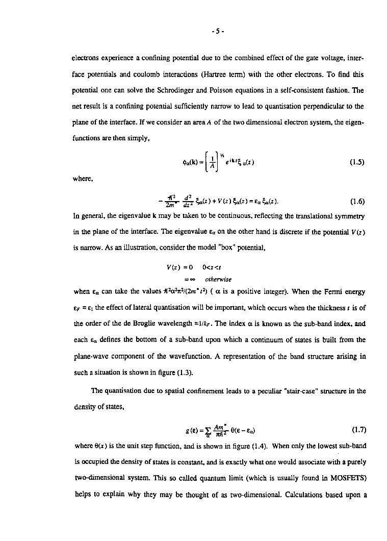
The quanti8ation due to spatial confinement leads to a peculiar "stair-case" structure in the
density of states,
g(£)=~ ~; 9(£-Ea) (1.7)
where 9(x) is the unit step function, and is shown in figure (1.4). When only the lowest sub-band
is occupied the density of states is constant, and is exactly what one would associate with a purely
two-dimensional system. This so called quantum limit (which is usually found in MOSFETS)
helps to explain why they may be thought of as two-dimensional. Calculations based upon a

ENERGY
Figure 1.3: A representation of the sub-~and structure for a given direction in k-space. The elE~trons occupy all the states up to the Femu level (at T = 0 ).
a) b)
en w
en ~ w ~ ~ :: IJl
I'- en 0 I'-
> 0 ~
> v; ~ z en w z 0 w 0
ENERGY ENERGY
Figure 1.4: a) The density of states in a MOSFET with several occupied sub-bands. b) A wideri MOSFET with many occupied sUb-bands. The envelope of the steps varies as E~, characteristic oP.' a 3D density of states. i
,

-6-
model of a simple 2DEG have proved to be very successful in discussing MOSFET physics
(Ando et al 1982). The most important feature of the system is that the electrons are essentially
free to move in only two directions. Details of the exact form of the sub-band wavefunctions and
the confining potential are. (at least from the point of view of transport properties) of lesser
importance. which is helpful since it permits simple models to be used with relative accuracy.
The same is also found to be true for the effects of exchange and correlation. and so the single
particle description is a reasonable basis with which to work. (There are of course situations
where this is certainly not the case. and a many-body description must be invoked. Probably the
most graphic illustration of this in a 2DEG is the fractional quantum hall effect (Laughlin 1983),
which is inherently a many-body phenomenon).
By increasing the gate voltage it is possible to draw more electrons into the inversion layer
and thus have more than one occupied sub-band. When several sub-bands are occupied we have a
region of quasi-two-dimensionality. in which the electrons are still free to move in the plane of
the layer. but inter-sub-band scattering generates an "effective" motion perpendicular to the inter
face. It is not hard to imagine that the singularities in the density of states (figure (1.4» will lead
to potentially novel behaviour in this regime. due for example to the changing scattering rates as
a function of Fermi level. In later chapters we shall look at phenomena of this kind. The three
dimensional limit is associated with a great many (closely spaced) sub-bands or equivalently,
with confinement channels that are very wide. Just what constitutes "wide" is a pertinent question
and will form a recurring theme throughout this work. The 2D to 3D crossover in the density of
states is demonstrated graphically in figure 0.4). The great advantage of using MOSFETS to
study 2D behaviour is that the Fermi level can be altered, which makes it possible to probe dif
ferent regimes within the same sample. There are other examples of quasi-two-dimensional sys
terns which have also proved useful in investigating 2D physics. and we mention some of these in
passing. The GaAs - AlGaAs heterojunction can confine electrons in a small layer near the inter
face because of band bending in the presence of an abrupt compositional change. Details of the
confining potential are different. but transport is similar to that found in MOSFETS (Ando et al
1982. Thornton et al 1986). Thin (deposited) films of metal and semiconductor often behave

-7-
two-dimensionally and have been especially useful in studying localisation phenomena (Berg-
mann 1984). Certain bulk solids can show aspects of low dimensionality due to strong spatial
anisotropy in the system, the well defined planes in graphite being a good example. Finally, it has
even proved possible to study electrons on the surface of liquid helium, where electrons have
very high mobilities, and where crystallisation of a 2DEG has been observed at sufficiently low
temperatures (Grimes and Adams 1979).
1.4 One dimensional systems.
Systems which are inherently one dimensional may be constructed in analogous fashion by
spatially restricting the electrons in two dimensions instead of one. A sub-band structure will
develop as in the MOSFET, although each sub-band will be labelled by two indices rather than
one. The resulting density of states is even more peculiar,
(1.8)
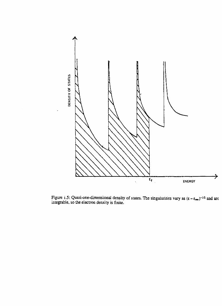
and is shown schematically in figure (1.5). The most interesting feature is the singularities which
occur when the energy coincides with a sub-band minimum. As it stands, we can expect more
exotic behaviour to arise in quasi- one-dimensional systems (compared to MOSFETS) because of
these singularities. Devices to potentially probe such behaviour have been made in a variety of
ways. Most of the early work concentrated upon constricting the 2DEG of a MOSFET in onc
more direction, either electrostatically (Fowler et al 1982), or by defining a narrow channel using
electron beam (Skocpol et al 1982 ) or optical (Wheeler et al 1982) lithography. In a similar
fashion, narrow channels may be defined in the 2DEG of a GaAs-AIGaAs heterojunction (Thorn
ton et al 1986, van Houten et al 1988). As lithographic teChniques have become more advanced,
it has proved possible to fabricate wires of sufficiently small cross-sectional area to observe
quasi-ID behaviour. A variety of materials have been used for this, such as AuPd alloy (Masden
and Giordano 1982), aluminium (Santhanam et al 1984), lithium (Licini et al 1985) and n+GaAs
(Whittington et al 1986). Wires which are free standing in space have also been fabricated, from
amorphous silicon nitride (Lee et al1984) and AuPd (Smith et alI985). Each of these devices is
slightly different and highlights different aspects of one-dimensional transport. Typical
.... o > '"" Vi z w C
Figure i.5: Quasi-one-dimensional density of states. The singularities vary as (£ - £IM till and are integrable, so the electron density is finite.

- 8 -
dimensions are lengths measured in microns and lateral dimensions measured in some hundreds
of angstroms; more will be said about this later. What is evident from the experiments is that
these systems can behave very differently from the way simple models suggest This raises a very
important question; is the model which works well in 30 and 20 wrong in lower dimensions, or
is there some new physics found in quasi-ID (and to a lesser extent quasi-20) systems which
masks the effect? Perhaps one such possible mechanism can be guessed at immediately, namely
the presence of statistical features associated with the small numbers of electrons and impurities in
such devices. We shall see that fluctuations are indeed an important facet of transport in
extremely small structures.
1.5 Localisation and fluctuation phenomena.
Studies of transport in low dimensional structures have also shown the importance of
disorder. Conventional transport theory is based upon the idea that plane wave states (which
have a well defined momentum) are capable of carrying current Scattering causes these plane
wave states to scatter into other plane wave states, which controls the size of the current induced
by an external stimulus. The scattering is not however considered to affect the nature of the elec
tron states, which remain extended throughout the sample. That things might not be so simple in
low dimensional systems became apparent after the pioneering work of Anderson (1958), who
showed that if the disorder (Le. impurity concentration) was strong enough, then the electrons
would become localised instead of extended throughout space. Pursuing this idea, Abrahams et al
(1979) predicted that all infinite 20 and 10 disordered solids will be insulators at T=O! Even for
finite sized systems the effect of this localisation significantly alters the behaviour of electron
transport, especially in one dimension. Localisation is a quantum phenomenon which is ignored
by conventional semiclassical transport theory, but is clearly an important factor in low dimen
sional physics. Although localisation effects are also present in bulk specimens, they are (usually)
considerably smaller, and so ignoring them does not lead to any noticeable inaccuracies.
In the previous section we touched upon the question of statistics in very small systems.
Al'tshuler (1985) and Lee and Stone (1985) have shown that such "mesoscopic" samples exhibit

-9-
very interesting fluctuation phenomena and sample specific propenies which are not evident in
larger samples. For example, the conductance of a given sample will show a reproducible, noise
like structure as a function of chemical potential or magnetic field. Such "Universal Conductance
Fluctuations" were initially observed by Umbach et al (1984) in small Au and AuPd rings and
wires, and have been reproduced many times since (Webb et al 1987). These fluctuations are
washed out as a function of increasing temperature and system size exactly as expected. At T=O,
they have universal behaviour which is independent of system shape and only weakly dependent
on the dimensionality. Like localisation, these fluctuations are a quantum phenomenon which
conventional theories (that calculate average quantities) overlook. Both of these effects, impor
tant in small structures and interesting in their own right, will be discussed in detail throughout
the rest of this thesis.
1.6 Applications in technology.
With the advent of microfabrication and the increasing degree of miniaturisation in sem
iconductor technology, electronic components are now reaching a size where quantum
confinement effects are becoming important in determining device performance. In addition, and
perhaps most excitingly of all, modem growth teChniques such as MOCVD (Metal Organic
Chemical Vapour Deposition) and MBE (Molecular Beam Epitaxy) have reached a degree of
sophistication where it is possible to grow specifically designed structures on the low dimensional
length scale (see Physics and Fabrication of Microstructures and Devices ed. KeUy and Wiesbuch
1986). It is then possible to imagine even incorporating the novel physics of quantum
confinement into the mode of device operation. These ideas have been explored in the review
articles by Board (1985), Kelly and Nicholas (1985), who have discussed for example the super
lattice and the quantum well laser, and by Bate (1988). In a series of papers, Capasso et al .
(1983a,1983b,1984) have discussed compositionally graded devices and pointed out the possibili
ties for negative differential resistance, switching and storing devices, photodetectors and pho
tomultipliers as well as diodes and transistors of various types. These ideas have been discussed
in more detail recently by Heiblum and Eastman (1987). Quantum interference devices based

- 10-
upon the Aharonov-Bohm effect have also been postulated (Bandyopadhyay et al 1986, Datta and
Bandyopadhyay 1987). Already certain of these structures are showing promising signs, and
improvement in device perfonnance can only get better as the physics of these ultra-small devices
becomes more clearly understood. By studying such devices theoretically we can attempt to see
which are the important features, and which are irrelevant as far as device application is con
cerned.
1.7 Outline of thesis.
In the previous sections we have discussed some of the important aspects of transport in low
dimensional (especially quasi-one-dimensional) systems. The rest of this thesis will focus on
investigating Lhese and additional features of electrical and thennal transport in such systems,
concentrating on quantum confinement effects, localisation and fluctuation phenomena. In
chapter 2, a simple Boltzmann method is used to further illustrate the ideas and to calculate the
effect of sub-blmd structure on the transport coefficients in a wire. In chapter 3, the full quantum
nature is introduced by considering a more sophisticated fonnalism based on Green function
techniques. The results of Chapter 2 are recalculated which explicitly demonstrates the impor
tance of lifetime broadening in these systems. Chapter 4 is a general review of the theory of local
isation and conductance fluctuations relevant to the remaining discussion. Chapter 5 presents a
calculation of the weak localisation correction in the quasi-one-dimensional regime, but as a
function of an arbitrary number of occupied sub-bands. This allows explicit demonstration of
finite width effects ignored in the usual treatments. In Chapter 6, the effects of localisation on the
thermal conductivity and thennopower are calculated both in the weak localisation regime and in
the vicinity of a Metal-Insulator transition, which leads to a highly plausible scaling theory of
thermal transport. Fluctuation effects in thermal transport are also calculated and demonstrated.
Finally, in Chapter 7, conclusions are given and possible outlines are presented on the prospects
for the future, such as ballistic transport, the relation of fluctuations to l/f noise, and problems
relating to measurement in ultra-small devices.

- 11 -
CHAPTER 2
BOLTZMANN TRANSPORT IN QUASI-ONE-DIMENSIONAL WIRES.
2.1 The transport coefficients.
Under conditions of equilibrium, the conduction electrons in a metal or doped semiconduc-
tor are distributed over their energy levels according to the Fenni-Dirac distribution function.
Upon applying an external stimulus (an electric field or temperature gradient for example), the
electron distribution will be perturbed away from its equilibrium value and, as a result, currents
defined on a macroscopic scale will begin to flow. Assuming these stimuli are small, we can
relate them linearly to the electric and heat current densities J and Q,
J =LlI E' -!:.p- VT (2.1a)
Q E' L22 V =L21 -""I T (2.1b)
where E' = E + I e I-I VIl. E is the applied electric field and Il the chemical potential. The L ~ are
characteristic of the system under consideration and are the quantities we wish to calculate. In
general they will be second rank tensors, a complication we shall ignore by restricting the discus
sion to systems with cubic symmetry where they reduce to scalar multiples of the unit tensor
(Butcher 1973). We can then relate the Lap to the commonly measured electrical conductivity <7,
the thennal conductivity 1C and the thennopower S by.
<7=LI\
1C = (L22 L 11 - L21 L 12)' (TL 1\)
S = Lu' (TLu).
(2.2a)
(2.2b)
(2.2c)
These quantities will be calculated for a quasi-one-dimensional model system when several sub-
bands are occupied. Within the framework of Boltzmann theory we shall see that this regime is
much more interesting than the one where only the lowest sub-band is occupied.
2.2 Boltzmann transport theory.
Boltzmann theory concerns itself with the calculation of the perturbed electron distribution
function. Although it treats the underlying dynamics very simply. it nevertheless provides intui
tive insight into an otherwise complicated problem (Greenwood 1958), and has proved very

- 12-
successful in analysing a wide range of phenomena in bulk semiconductors and metals (Blatt
1968, Nag 1980, Butcher 1986). Since the method is well known, we shall content ourselves
with only a brief description. The central idea is that since electrons cannot be destroyed, the per-
turbed distribution function I (k.r J) must obey a continuity equation of the following type,
(J[ +v.Vr/ - le I E'.V",I = [Of] Tt -r Tt coli
(2.3)
Equation (2.3) represents the competition between the applied fields which tend to drive the sys
tem away from eqUilibrium and scattering (contained within the collision term) which tends to
restore it. Since impurity scattering dominates at low temperatures (where most of the interesting
effects are observed) we shall consider this particular mechanism in detail. The word impurity
will be used somewhat loosely, it could refer to donor atoms for example or equally well to
defects and disorder within the solid. All such static deviations from periodicity will scatter the
electrons elastically, which further simplifies the analysis. Once we have calculated the distribu-
tion function for a particular model, the electric and heat current densities are given by (Butcher
1973, 1986),
J le I ~f ' =---~ va.la. dk 1t a
Q= ~ ~f va.(£-lL)/a. dk' a
(2.4a)
(2.4b)
We shall also assume that steady state has been attained, and leave it understood that if I is an
explicit function of the variable r, then equations (2.4a) and (2.4b) represent the current densities
at the point r. The index a is a band index, and in the present problem refers to the sub-bands.
2.3 The quasi-one-dimensional regime.
In a quasi-ID system, the electrons in the (m.n )th sub-band will be described by a distribu
tion function I"", (k .r), each of which will obey an equation of the type (2.3). The collision term
must account for scattering between the sub-bands as well as scattering within the same sub-band,
and so we write,
[¥t] = I; f [P (k'ij;kmn) /;j(t') (1-1"", (k» coli '')
(2.5)
- P(kmn ;k'ij) I"", (k) (l-lij(k'»] iit dk'
- 13-
where P (kmn ;k';j) is the transition rate from a full state Ikmn> to an empty state I k'ij >. The first
tenn accounts for scattering into the state I kmn > and the second for scattering out of it Equations
(2.3) and (2.5) then provide a set of coupled equations for the distribution functions. To solve
them we make a number of approximations of a standard type (Butcher 1973. Nag 1980). Firstly
we note that since the scattering is assumed to be elastic. detailed balance implies.
P(kmn ;k'ij) = P(k'ij;kmn) (2.6)
Secondly. by asSUII'ing the fields are weak we can line arise I by writing.
(2.7)
where 10 is the Fermi-Dirac distribution and I..!.. is a small correction which is linearly related to
E' and VT. TIllrdly. we can employ the relaxation time approximation (strictly valid for elastic
scattering and symmetric energy bands).
[aLl - I..!.. Tt coU - - 't"", (2.8)
't ..... is an energy dependent relaxation time which characterises the electron-impurity interaction.
Within these three approximations we find.
f..!.. = 't/llll v ..... [I e lE' + + 1[; (E;.t)] a/EO (2.9)
v ..... is the velocity of an electron in sub-band (m.n) with wavevector k. We are going to assume
that the sub-bands are parabolic. whereupon VIM =-Ifklm· = (2(E-t ..... )lm· )\ofa. It is of course possible
to include non-parabolic effects (Nelson et al 1987). but we expect the effect on the transpon
coefficients to be small unless the non-parabolicity in unusually large. The relaxation times are
given by.
-t1 = r.I P(kmn;k'ij)..!;. dk' - r.I P(k'ij;kmn).3JL Tk' ...!= dk'. ..... I.) "'~ I.) t_ '''It
(2.10)
There are several points which should be stressed about the relaxation times. In the case of
multi-sub-band transport they are generally coupled together because of inter-sub-band scattering
(Siggia and Kwok 1970. Milsom and Butcher 1986). Secondly. the relaxation times are not the
scattering times of plane wave states (we shall return to this shortly). Finally. they are only
independent of temperature because we have assumed the scattering to be entirely elastic. There
are various subtleties associated with elastic scattering which must be handled carefully. and we

-14 -
shall address them as they are encountered. In the presence of inelastic scattering equation (2.10)
would explicitly contain the Fenni function.
The relaxation times may be calculated once the transition rate is specified. For this we use
Fermi's Golden Rule:
P (kmn ;k'ij) = 1:;- 1 <kmn 1 VI k'ij > 12 o(e-e') (2.11)
which requires the fonn of the wavefunctions in the absence of disorder and the impurity poten-
tial to be known. Clearly for a qualitative discussion of transport through a device, the exact fonn
of the sub-band wavefunctions is less important than the fact that there are discontinuities in the
density of states (although this is not necessarily true for other quantities such as optical absorp-
tion for example). We therefore content ourselves with a model confining potential of the infinite
"box" type where,
,,_(k): [ rlFj" ,ih ,in(nula) ,in(mKylb) (2.12)
and a and b are the channel widths in the x and y directions of a wire of length L (L » a ,b ).
More sophisticated calculations have been performed (Berggren and Newson 1986, Laux et al
1988) and show this basis set is a reasonable one. The simplest fonn of scattering which is elastic
and pointlike is of the standard 0 - function type,
V (r) = ~ U 0 O(r-r.) (2.13)
where r. is the position of the Ith impurity and U 0 is a measure of the strength of the interaction.
o - function scatterers have the nice, additional feature of being velocity randomising in the sense
that scattering to another sub-band is equally favoured to states k and -k in that sub-band. The
last term in equation (2.10) is then zero and the equations decouple (a similar effect occurs in 3D
systems and is well known (Butcher 1973». The transition rate however still depends upon the
positions of all the impurities. This dependence may be removed by assuming the system is
sufficiently large and the impurity coordinates sufficiently uncorrelated that we can average over
all possible impurity configurations. This ensemble averaging was first discussed in detail by
Kohn and Luttinger (1957). The fundamental assumption behind it is that the mean behaviour of
all macroscopically similar samples is the same as the typical behaviour of a given sample.

- 15 -
Naturally this neglects fluctuation effects such as Universal Conductance Fluctuations (Lee et al
1987) and we will return to discuss these later. Configuration averaging (by integrating over the
impurity coordinates) assuming the density of impurities is small gives,
1 -2 [ Uo J2[m.J~~ (2+Ojm)(2+~jll)e(£-£ij) -:-r:::\ - no ~ ~ ~ ()'A t"", \£) .t;TlUO ~ I J £-£jj
(2.14)
where no is the number of scatterers per unit length. It should be noted that in the limit a or b
tending to zero the right hand side of this expression appears to diverge. This is an artifact of 8 -
function potentials; for a potential with a finite range R the relaxation times become independent
of a and b in the limit a «R, b «R as may easily be verified. There is no problem however in
discussing the physical behaviour of the transport coefficients by using zero-range scattering
potentials.
A schematic plot of the relaxation times as a function of energy in the lowest three sub-
bands is shown in figure 2.1. The behaviour one would associate with a purely 10 system,
namely t N £~ is clearly visible in the lowest sub-band. When e coincides with a sub-band
minimum however, the relaxation times drop discontinuously to zero. This reflects the fonn of
the quasi-ID density of states (figure 1.5), since at each new sub-band minimum there is an
infinite density of states for the electrons to scatter to. This structure in t(e) is more pronounced
than that found in 20 structures (see e.g. Mori and Ando 1979, Semelius et al 1985», precisely
because the density of states shows sharper discontinuities. Since the transport properties of the
system depend upon t(e), we should therefore expect to see considerable structure in the transport
coefficients as the chemical potential is varied. This structure will be evident in the vicinity of the
sub-band minima, irrespective of the actual value of the energies of these minima, which is
a.,other reason why the exact sub-band wavefunctions do not need to be known.
2.4 The electrical conductivity.
Having found the perturbed distribution function, we can insert it into equations (2.4a) and
(2.4b) to derive expressions for the electric and heat currents. Comparison with equations (2.1a)
and (2.1b) directly leads to the Laf, and hence the electrical conductivity, thennal conductivity
and thermopower. We find,

<J) w ~ ~
z o
~ x et ...... w Cl::
I
5 10
, ,
,-..., . ..,. ,...-:;-- . , , -'
. ", '", . ~ "
/"
ENERGY / meV
Figure 2.1: A schematic plot of the relaxation times of the lowest three sub-bands as a function of energy. The second sub-band minimum is at 5 meV. the third is at 10 meV.
1
80
-is 6 -' t! ...
./ '2 ... )(
.....
> != ,., >
, \
~ \
U .< :l "./ \ 0 Z / 0 40 ,/ u ,/
5 10
CHEMICAL POTENTIAL I meV
Figure 2.2; The conductivity as a function of chemical potential for three different temperatures andlcFl =30:--T =O.3K ,-------T =3K and -'-'-'T =30K .
-16 -
Lll = I a(e)(-o/O'oe) de
L 12 = L21 = - -rtr I aCe) (e-l.1) (- a/O(oe) de
L22= ~ I aCe) (e-I.1)2 (- a/o/ae) de
where,
a(e) = I: n/M (e) e! 't/M (e) m", m
and,
(2.1Sa)
(2.1Sb)
(2.1Sc)
(2.16a)
(2.16b)
There are several interesting features to these results. Firstly, since Lll is equal to the conduc-
tivity, and at T::O, of 10e = -i>(e-eF), a(eF) in the above equations is simply the zero temperature
conductivity of the system. Correspondingly, n/M (£F) is simply the density of electrons in the
(m,n)th sub-band (compare equation (2.16a) with the 3D result, equation 0.1». Secondly, the
function aCe) enters the expressions for all the Lalh and so the thermal transport coefficients are
intimately related to the electrical conductivity. This is not accidental as will be explained in sec
tion 3.5. The third very important result is that L 12 = L2lt which is guaranteed by an Onsager rela
tion (Butcher 1986) and is not just a consequence of the relaxation time approximation. We will
find this a useful identity when we come to discuss the thermopower in a little more detail.
We will consider a representative system with sub-bands separated by a typical energy of
order 5 mev (Semelius et al 1985). The effectiveness of the scattering depends upon the impurity
density no and their strength Vo, and may be characterised by specifying the dimensionless
number kFl for some value of kF ( kF is the Fermi wavevector and I is the mean free path at the
Fermi surface). The value of kF I we shall quote is for a Fermi energy of 2.5 mev, half way up the
ground sub-band. Later we shall find it more convenient to specify the disorder through the sam
ple mobility, in order to compare with experiment Notice that larger values of kFl refer to less
disorder. The conductivity is plotted as a function of chemical potential for several different tem
peratures in figure (2.2). When the temperature is low, the conductivity drops when 1.1 passes
through a sub-band minimum due to the increased scattering (recall the behaviour of the relaxa-
tion times). Such features in the transport coefficients are known collectively as quantum size

-17 -
effects or QSE. As the temperature is raised, thermal broadening becomes more important until
when ks T is comparable to the sub-band separation all the structure is smeared out ( 5 mev
corresponds to approximately 30 K). In this regime, a is almost linear in J..L and all information
about the sub-bands is lost. This explains incidently why experiments have to be performed at
low temperatures ifQSE are to be observed. We have not plotted the conductivity as a function of
disorder ( kFl ), since in Boltzmann theory a is simply proportional to kFl or inversely propor
tional to the impurity concentration.
The above calculation is very simplistic and supports our conjecture that sub-band structure
should lead to QSE in the conductivity. This idea is not new, and has been anticipated in 20 sys
tems for a long time (Mori and Ando 1979, Sernelius et al 1985, Milsom 1987). Inclusion of ine
lastic scattering via phonons for example does little to change the structure of the results (Fish
man 1987, Milsom and Butcher 1986). Comparison with experiments produces in general, how
ever, very poor agreement. The most suitable device for performing the experiments on is the
pinched MOSFET (see introductory chapter), since it allows the chemical potential to be varied
continuously. In the experiments carried out by Skocpol et al (1984), some tantalising evidence
for QSE was observed but was very inconclusive. Further experiments on devices with greater
resistance (and hence more disorder) (Hartstein et al 1984) produced even less agreement, with
marked (though reproducible) ftuctuations being apparent. In an effort to reduce the effect of
these ftuctuations (to try and resolve sub-band structure in the conductivity), Warren et al (1986)
performed an experiment on 250 parallel inversion lines simultaneously, and produced perhaps
the best evidence for QSE in quasi-ID conduction. What is very clear however is that the size of
the effect is very much reduced from the Boltzmann predicted values, and that the role of increas
ing disorder is much more important than this simple theory would have us believe. To treat
quasi-one-dimensional systems properly we are therefore going to have to go beyond simple sem
iclassical theories.
2.5 Thermal transport in sub-band systems.
It is useful to calculate the thennal transpon coefficients within the Boltzmann framework

!le: 20 .... E -;; ~
~ '2 16
)(
" > !:: > ;::
12 u ::l C Z 0 U
-' < 8 lE D:: w Z ~
4
5 10
CHEMICAL POTENTIAL I meV
Figure 2.3: The thennal conductivity of the same system for the same three temperatures as in the previous figure.
80
40 !le: \ .... I \ > I \ :1- I "- / D:: w / ~ / .- -.-0 ,/ -~
, . \
'- ..... 0 ... -_." .-lE / D:: -40 .... Z ~
CHEMICAL POTENTIAL I
-80
.-... , , ..
.-.. /'
'" '"
Figure 2.4: The thennopower as a function of chemical potential for, --T = O.3K • - ·_·-T=3K and ··· ·· ···T=30K.
meV
- 18 -
to compare with later results. Some calculations have been performed in the pure 10 regime for
these coefficients (Kubakaddi et al 1985, Jali et al 1987a, 1987b) but as we have stressed, the
more interesting regime is when several sub-bands are occupied. The thermal conductivity 1C is
plotted in figure (2.3) as a function of Il, again for several values of T. The first point is that 1C is
always positive, a consequence of the second law of thermodynamics. Like a, the thermal con
ductivity also exhibits QSE which are gradually washed out by thermal broadening at higher tem
peratures. It is interesting to note that at higher temperatures both 1C and a are approximately
linear in Il, which nicely supports the Wiedemann-Franz law (equation 1.3) both in scaling and
magnitude. The thermopower S on the other hand shows a very different type of behaviour to a
and 1C (figure 2.4). When Il is near a sub-band minimum, S may even change sign (Cantrell and
Butcher 1985a) and in general varies more rapidly with Il than either a or !C. The magnitude of the
positive peaks is also rather large (of order 70 IlVK-1 ). This suggests that if we wish to observe
QSE, then the thermopower is the best quantity to measure being so sensitive to the sub-band
structure in the system. The two other interesting features about the thermopower are its indepen
dence of both the degree of disorder in the system and also the effective mass m· . This leads us to
suspect that the thermopower may have certain universal features independent of the material
used in the experiments (we shall see later than in some respects this is indeed true), which
should be readily verifiable.
The fact that the thermopower can have either sign is of course well known, though the
mechanisms by which a change in sign arises are hardly ever discussed. This is because in order
to explain the change in sign of the coefficient L 12, it is necessary to think about how almost
degenerate electrons couple to a temperat1Jre gradient, which is generally hard to do. Fortunately
there is a way of getting around this problem. The Onsager relation L 12 = L 21 provides a con
venient identity in this respect, since if we can explain any sign change in Lu we will have
accomplished our task. This coefficient defines the rate of heat transport in the presence of an
electromotive force rather than a temperature gradient (equation 2.tb), and is conceptually easier
to think about. Consider a Fermi sea of electrons. At finite temperature a certain number will be
excited above the Fenni surface, leaving some hole-like excitations below it. When an electric

-19 -
field is applied. the electrons and holes drift in opposite directions but since they have opposite
charge. they both contribute to the current in the same sense. The conductivity is thus always
positive. When we talk about heat transfer however. the electrons and holes carry heat in opposite
directions. When kg T is small these two contributions nearly cancel. Normally. the heat flux due
to the electron-like excitations will be slightly greater than the heat flux transported by the holes
(in the opposite direction) because the electrons have slightly greater velocity. If the Fermi level
lies just below a sub-band minimum however. the electrons will experience a rapid increase in
scattering compared to the holes because their excited energies lie in the region of this minimum.
They therefore transport heat far less effectively and the hole contribution takes over. The
coefficient L21 changes sign in this case. and as a result, so does the thermopower. Having seen this
argument we can now understand why the coefficient L 12 might change sign. When a temperature
gradient is applied (in the absence of any electric fields). the electrons and holes both drift in the
same direction (from hot to cold) and the two contributions to the electric current nearly cancel.
The argument for the sign change then goes through exactly as before.
To see how long these positive peaks stay in the therrnopower. we should calculate S UL.T)
as a function of temperature rather than chemical potential. When doing this. it should be remem-
bered that ~ is also a function of T. because the number of electrons in the system remains con-
stanL This is often overlooked. The variation ~(T) may therefore be calculated numerically from.
(2.17)
where the number of electrons N is determined from the Fermi energy ( £F = ~(O) ) in the limit
T -+0. Several results for ~(T) are shown in figure (2.5). The variation of ~ is most pronounced
when £.F lies just below a sub-band minimum; the proximity of the next sub-band means there is a
large number of states with £. slightly greater than £F for the electrons to occupy as T is raised.
which makes I.l fall off rapidly. Taking the temperature dependence of ~ into account. S is plotted
as a function of T for two values of £F in figure (2.6). Near a sub-band minimum we can expect
positive thermopower to persist up to T <6K. When £.F is many kg T away from a sub-band
minimum • S is negative and linear in T, and is well represented by the usual Mott formula (equa-

0 .1
~ -0.1 E
" -w
- 0.3
-0.5
" ... , , , " ,
" "
B
" , ...
.-. 3
... ... ... ... ...
'-'-'- '
... A ' ............
.......
.-.-.-. c
' - ' -'- ''-'- ' -
6
TEMPERATURE I K
Figure 2.5: The deviation of the chemical potential from the Fermi energy as a function of temperature. for three different values of the Fermi energy EF A) 4.9 meV. B) 5.2 meV and C) 7.5 me V. The second sub-band minimum is at 5 me V.
:a:: " 20 5-" ~ TEMPERATURE I " w ~ 0 ~ 0 ~ ~ w :z:: ....
-20
Figure 2.6: The thermopower as a function of temperature for two different values of the Fermi energy A) 4.9 meV and B) 7.5 meV. and kd = 30.
- 20-
tion (l.4». Although we have only perfonned the calculations for the lowest three sub-bands, all
the ideas discussed above will hold in higher sub-bands. In particular, we expect to see a positive
contribution to the diffusion thennopower in the region of all sub-band minima as long as k8 T is
considerably less than the sub-band separation.
Experimental measurement of the thennopower of low dimensional structures is being per
fonned more and more, despite the difficulties involved. Although no measurements have been
carried out for quasi-ID systems, promising results are now being obtained in 20 and in silicon
microcontacts (Davidson et al 1986, Retcher et al 1986, Gallagher et al 1987, Trzinsld et al 1986.
Ruf et al 1988), as well as some intriguing observations in graphite (Sugihara et al 1986)
reflecting the strong spatial anisotropy of this system. No concrete evidence for QSE has yet
been universally found (the experiments so far have not generally been looking for them), though
very recent experiments have shown a change of sign of the type expected (C.Ruf private com
munication). It has been demonstrated, however, that phonon-drag (which we have ignored) is
also important. (In the experiments of Ruf et al they subtracted this phonon-drag component from
the total result in order to show a sign change in the diffusive component of the thennopower).
Simple calculations for the phonon-drag thennopower in 'ID have been perfonned (Nicholas
1985, Cantrell and Butcher 1987a.b), and the agreement with experiment is encouraging. The
expectation however is that the diffusive component of S we have calculated and the phonon
drag components will be additive, and so experiments designed to look for QSE are still well
worth performing. especially in wires where the effect is expected to be largest Work is currently
underway to further understand phonon-drag in low dimensional structures.
- 21 -
CHAFfER 3
LIFETIME BROADENING OF SUB-BAND STRUCTURE.
3.1 Introduction to lifetime broadening_
We have discussed Boltzmann transport theory in a quasi-one-dimensional wire, and found
that the results for the conductivity do not agree well with experiment We therefore need to
improve the theory and go beyond the simple approximations that the Boltzmann method
assumes. Hopefully we will find that some of the features highlighted in the previous chapter will
persist and surface also in a more sophisticated treatment.
Certainly one approximation that Boltzmann theory relies on, namely that the scattering
does not affect the single particle properties such as the nature of the electron states between col
lisions or the density of states, must be considered dubious. On general quantum mechanical
grounds, a state characterised by a lifetime t has a natural uncertainty in its energy;vtf It, and this
broadening must modify the single particle properties. For weakly disordered 3D systems this
effect is usually small, and correspondingly the Boltzmann method often works quite well. For
low dimensional systems on the other hand this need not be the case at all (Cantrell and Butcher
1985b). One consequence of this will be that the QSE in the transport coefficients are consider
ably reduced when broadening is introduced into the theory.
Our aim then is to develop a systematic theory which may be applied to a quasi-one
dimensional wire and which implicitly allows for broadening. This is achieved using Green's
function methods and standard field theory techniques. Unlike most other workers we choose to
work at finite temperature at the outset through the Matsubara method. The results obtained will
also be of considerable use later in this work. An approximate calculation will then be performed
and for the purposes of comparison, the results of the last Chapter are recalculated. For general
accounts of the methods used the reader is refelTed to standard texts e.g. Abrikosov et al 1965,
Fetter and Walecka 1971 or Mahan 1981. The book by Nakajima et al1980 provides an excel
lent introduction to the ideas of Fermi-Liquid theory, and at a simpler level, an illuminating dis
cussion of the impurity problem is given by Doniach and Sondheimer 1974. The specific

- 22-
question of doping effects on the electron states in semiconductors has been addressed by
Bonch-Bruevich 1966.
3.2 The single-particle Green's function.
The model used previously for the unperturbed system provides a convenient set of basis
states for the calculation. Introducing the field operators,
\jI(X) = b Il>IIk (x) C Ilk
'f"(x) = b ,~(x) C c1t
the N-electron Hamiltonian may be cast into second quantised form,
(3.1a)
(3.1b)
1 1 . H = r ~ f:lf2k2/2m· + ea) C+1Ik C Ilk + r ~. M c4i(X"Y"q) eU(Z' CctA:+q Cp.A: (3.2)
tit a,1f.r' .q .1
Map(X"Y"q) = f ~ U(x-X"y-Y"q) ~Il tU dy
with U the potential of the llh scatterer and q the wave number of the Fourier transfonn of the z
coordinate. For convenience the sub-band labels are labelled by one index a, and the spin labels
suppressed. The single particle Green's function which describes the excitations at finite tempera-
tures is,
Gc4i(k, k';t) = - <T" C pt' (t) C ctt (0) > (3.3)
where < .... > denotes the thermodynamic average over the N-particle states of the system.
(Further discussions and details may be found in Appendix A). Equation (3.3) may be Fourier
transformed to give a more useful representation (Mahan 1981),
(3.4)
The Matsubara frequencies for Fermions are odd; Pit = (2n + 1)1tI~ with ~ = lIks T, and contain
infonnation about the temperature of the system.
The (real-time) retarded Green's function may be obtained from the Matsubara function by
making the analytic continuation to the real axis ipIt -+ £+i 3 (see Appendix A). The variable £ is
an energy variable with domain -00<£<00, and is measured relative to the natural energy origin
which is the chemical potential. As in a general Fenni-Liquid theory, £ describes the energy of an
excitation in the system; those with £>0 are then quasi-particles and those with £<0 quasi-holes.

- 23-
Many useful properties of the system are given by the retarded (and advanced) Green's functions.
For example, the single-particle density of states is related to the diagonal components of GR (see
Appendix A),
g(E)=-! bImG~(k,k.E)
Another quantity of interest is the spectral function A u(k .E) defined by,
Aa(k.E) =-2 Im Gb(k. k ,E)
(3.5)
(3.6)
which is interpreted as being the probability that an excitation labelled by I k , u> has energy E. It
thus has an associated conservation law,
(3.7)
which is also shown in Appendix A. Not only are GR and GA useful in determining the equili
brium properties, we shall see that they are also related to the transport coefficients in the linear
response regime.
The second term in the Hamiltonian (3.2) represents the perturbation due to the impurities.
To evaluate the Green's function systematically in the presence of this perturbation, we write it in
the form,
G (k l' )=_ <T't[S«(3)C~t)Citt(O)l>o ~ , ,t <S »0 (3.8)
where < .... >0 now denotes a thermodynamic average over the unperturbed states of the system,
and the operators are defined in the interaction representation. Expanding the S - matrix, S «(3),
produces an infinite number of terms which may be conveniently represented graphically using
Feynman diagrams. The important diagrams are those which when summed. yield the proper
self-energy (Fetter and Walecka 1971, Mahan 1981) which is related to the Green's function via a
Dyson equation. The self-energy I has several important mathematical properties which hold
irrespective of the form of the perturbation (Nakajima et al 1980). If we regard ~ (k, k', Z) as a
function of the complex variable z. then I is analytic except on the real axis. Furthermore. the
real axis is a branch cut of the function such that the analytic continuation Z -+ xii a (x real)
yields.

- 24-
l:(Z~x± H» = 6(x).f ir(x) ,r(x»O (3.9)
where the real pan 6(x) shifts the energies of the excitations and the imaginary part r(x) deter
mines their damping. The imaginary part is the most important in determining the transport pro
perties of a given system because it directly relates to the scattering within the system.
The self-energy is configuration averaged to remove the dependence of the impurity coordi-
nates (Kohn and Luninger 1957, Edwards 1958). For a 3D system on a macroscopic length scale,
this implies the system is homogeneous (and as such translationally invariant), whereupon the
self energy and hence Green's function will be diagonal in k (Abrikosov et al 1965). For a sub
band system, impurity averaging still leads to !: and G being diagonal in k, but not in the sub-
band indices (because of the lack of translational symmetry in the confined directions). As a
result, the Dyson equation in general is of the matrix type,
G aP(k ,ip,,) = G g (k ,ip" )oaP + ~ G g (k ,ip" ) I.a:.l.k ,ip" ) G lII(k ,ip,,) y
where G g is the unperturbed Matsubara function,
Gg(k ,ip,,) = i t ~ 'p" -
~a.t = fj 2k 2/2m· + tu - ~
(3.10)
(3.11)
For impurity scattering, the proper self-energy has contributions of the following type after
configuration averaging (Mahan 1981),
+ *' I , , , I ,
I , I \
* ,,' , I "
" I ' " I '.,
+ _ ..
ok yk ok A q v yk ok yk ~ ~
I , , \
+ I \ . , + , \ I \ , , , I . \ , . J ) \ ,
yk ok
A cross represents scattering from a single scatterer, a dotted line denotes an electron-impurity
interaction which carries the appropriate matrix element and a full line is the full (perturbed)
Green's function. Since the scattering is taken to be elastic, all the Green's functions in the
diagrams have the same frequency ip", and so when evaluating the self-energy there are no fre
quencies summations to be performed. In principle we can now sum all the self-energy diagrams
and derive the exact Green's function through equation (3.10). This is of course impractical, and
- 25-
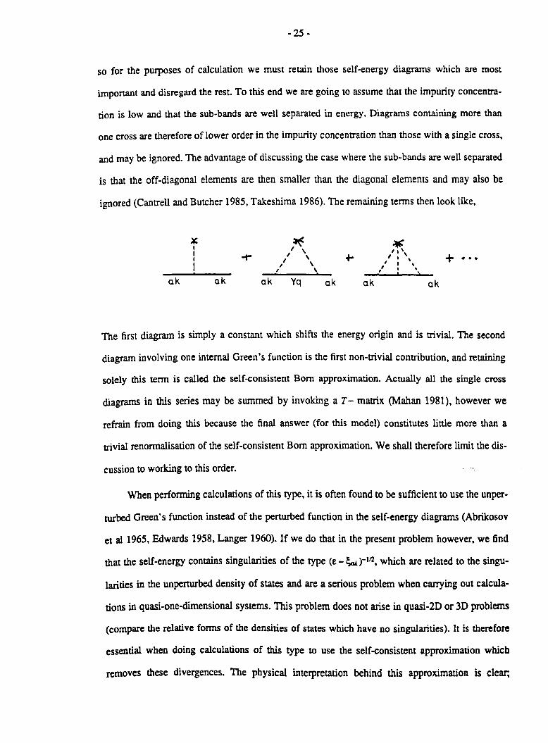
so for the purposes of calculation we must retain those self-energy diagrams which are most
imponant and disregard the rest. To this end we are going to assume that the impurity concentra
tion is low and that the sub-bands are well separated in energy. Diagrams containing more than
one cross are therefore of lower order in the impurity concentration than those with a single cross,
and may be ignored. The advantage of discussing the case where the sub-bands are well separated
is that the off-diagonal elements are then smaller than the diagonal elements and may also be
ignored (Cantrell and Butcher 1985. Takeshima 1986). The remaining tenns then look like,
X ,~ ~ I I -t- I ' +- '1\ + I
I ' , 1 , ' ..
I I , I I \ I , \
, 1 \ I , , , , I
ok ok ok Yq ok ok ok
The first diagram is simply a constant which shifts the energy origin and is trivial. The second
diagram involving one internal Green's function is the first non-trivial contribution, and retaining
solely this tenn is called the self-consistent Born approximation. Actually all the single cross
diagrams in this series may be summed by invoking a T- matrix (Mahan 1981), however we
refrain from doing this because the final answer (for this model) constitutes little more than a
trivial renonnalisation of the self-consistent Born approximation. We shall therefore limit the dis-
cussion to working to this order.
When performing calculations of this type, it is often found to be sufficient to use the unper-
turbed Green's function instead of the penurbed function in the self-energy diagrams (Abrikosov
et al 1965, Edwards 1958, Langer 1960). If we do that in the present problem however, we find
that the self-energy contains singularities of the type (t -I;a.t )-1/2, which are related to the singu
larities in the unpenurbed density of states and are a serious problem when carrying out calcula
tions in quasi-one-dimensional systems. This problem does not arise in quasi-2D or 3D problems
(compare the relative fonns of the densities of states which have no singularities). It is therefore
essential when doing calculations of this type to use the self-consistent approximation which
removes these divergences. The physical interpretation behind this approximation is clear;
- 26-
between collisions electrons are not free but move in the background potential of all the other
scatterers and are consequently damped (Langer and Neal1966). The Green's function and self-
energy must then be solved self-consistently retaining the same degree of approximation for both.
Within all these approximations we then have,
(3.12a)
(3.12b)
where < .... > means an ensemble average of the matrix elements M')6 given in equation (3.2), and
no is the impurity concentration per unit length. These quantities will now be calculated for the
model wire considered in the previous chapter.
3.3 The single particle density of states.
The evaluation of this self-energy is still not an easy task. To facilitate the calculation we
will therefore make one last approximation and justify it later. The real part of the self-energy
which shifts the energy of the excitations is usually small and so will neglect iL The imaginary
component. r, may then be calculated itemtively from equation (3.12b). For the ~ function scatter-
ing potentials, the averaged matrix elements are k independent and so the self-energy is depen
dent only on the sub-band labels and on the energy. The quantity of interest is the retarded self-
energy (which may be obtained from the above through the analytic continuation ;PII -+ £ + i 6 ).
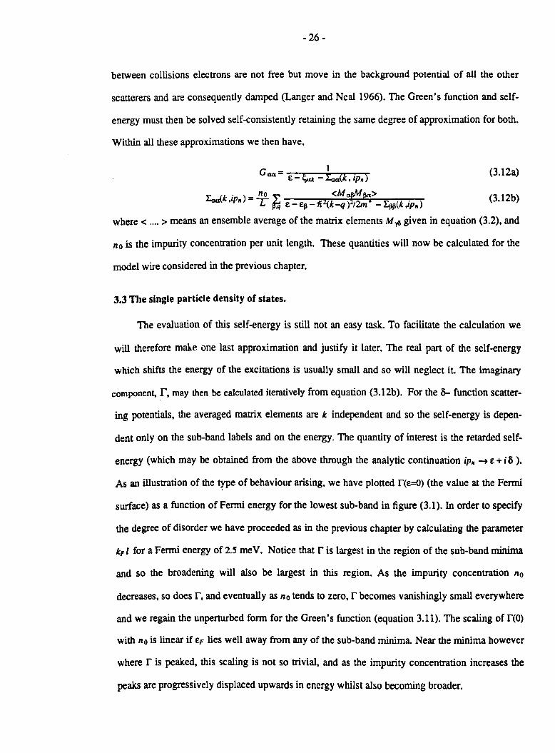
As an illustration of the trPe of behaviour arising. we have plotted n£=o) (the value at the Fermi
surface) as a function of Fermi energy for the lowest sub-band in figure (3.1). In order to specify
the degree of disorder we have proceeded as in the previous chapter by calculating the parameter
kF I for a Fermi energy of 2.5 me V. Notice that r is largest in the region of the sub-band minima
and so the broadening will also be largest in this region. As the impurity concentration no
decreases, so does r, and eventually as no tends to zero, r becomes vanishingly small everywhere
and we regain the unperturbed form for the Green's function (equation 3.11). The scaling of nO)
with no is linear if £F lies well away from any of the sub-band minima. Near the minima however
where r is peaked, this scaling is not so trivial, and as the impurity concentration increases the
peaks are progressively displaced upwards in energy whilst also becoming broader.

....
""" >-
0.5
~ 0.25 z ~ ~ :lE
5 10
CHEMICAL POTENTIAL I. meV
Figure 3.1: Imaginary part of the self-energy in the lowest sub-band as a function of cbemicat potential for A) kFJ = 30 and B) kFJ = 5.
u. o >-!:: In 2-.... Cl
.1
5 10 CHEMICAL POTENTIAL I meV
Figure 3.2: The single-particle density of states as a function of chemical potential A) kF 1 = 30. B) kFl = 5.
- 27-
Having found r(e) we can now calculate the single particle density of states. Before doing
so, we must be clear about the interpretation of the energy variable e. In a general theory, £ is sim-
ply an energy characteristic of the excitations which has no real physical significance, beyond
that of a dummy variable which is summed over to derive the physical quantities of interest
(Bonch-Bruevich 1966). For the present problem where the electrons are non-interacting how-
ever, we can identify the density of states at the Fermi level ( e = 0 ) as the analogous expression
to the unpenurbed density of states discussed in the previous chapter for the single electron prob-
lem. The broadened density of states (calculated from equation (3.5) ) is ploned in figure (3.2) for
two values of kFl. For a large value of kFl, the system is pure. r is therefore small and the density
of states is similar to the unperturbed form (figure l.S). To demonstrate the Boltzmann limit
analytically, we note that r -4 ()+ as kFl -4 00• so we may replace Im G§..(k .e) by - Jt 0 (e - ~a.t)
whereupon,
g (e) = ~ () (e - Sa.t) (3.13)
(£=0) = b. [ m· J ~ ~ O(eF-ea) g 1t 21f2 fi' (eF-£a)""
which is precisely the free electron form (equation 1.8). Notice however that the singularities
only occur in the actual limit no = O. As kFl decreases, the effects of the broadening become
apparent and the sub-band structure becomes less well defined. Eventually there comes a point
where the typical size of r is of the order of the sub-band spacing, and the density of states
becomes featureless. At this point it no longer makes sense even to think. about sub-bands
because they are so poorly defined. Clearly in this case the QSE in the transport coefficients will
also have vanished and the Boltzmann formalism (based on the idea of well defined sub-bands)
will have become completely invalid.
Many approximations used in deriving these results were rather crude, and so we should be
sure that the results derived are not simply a consequence of these approximations. Fortunately,
subsequent calculations which are more sophisticated tend to support these results quite well. Oas
Sarma and Xie (1987) use the same method as outlined above, but for a realistic screened
electron-impurity interaction. Their results are qualitatively very similar. Takeshima (1986) con-
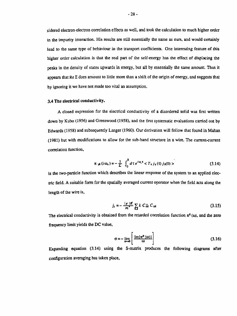
- 28 -
sidered electron-electron correlation effects as well, and took the calculation to much higher order
in the impurity interaction. His results are still essentially the same as ours, and would certainly
lead to the same type of behaviour in the transpon coefficients. One interesting feature of this
higher order calculation is that the real pan of the self-energy has the effect of displacing the
peaks in the density of states upwards in energy, but all by essentially the same amount Thus it
appears that Re I does amount to little more than a shift of the origin of energy, and suggests that
by ignoring it we have not made too vital an assumption.
3.4 The electrical conductivity.
A closed expression for the electrical conductivity of a disordered solid was first written
down by Kubo (1956) and Greenwood (1958), and the first systematic evaluations carried out by
Edwards (1958) and subsequently Langer (1960). Our derivation will follow that found in Mahan
(1981) but with modifications to allow for the sub-band structure in a wire. The current-current
correlation function,
(3.14)
is the two-panicle function which describes the linear response of the system to an applied elec-
tric field. A suitable form for the spatially averaged current operator when the field acts along the
length of the wire is,
jz =- 1~!1f' bk CJ.t Ca}( (3.15)
The electrical conductivity is obtained from the retarded correlation function 7r.R (00), and the zero
frequency limit yields the DC value,
(3.16)
Expanding equation (3.14) using the S-matrix produces the following diagrams after
configuration averaging has taken place,

- 29-
+ ...
where the full lines are damped Matsubara functions and the off-diagonal terms are once again
taken to be small. The rules for these diagrams are exactly the same as for the self-energy
diagrams. These two-particle terms describe the correlation between panicle-like (upper line) and
hole-like (lower line) excitations propagating in the presence of disorder.
The upper series of diagrams shown in this particle-hole channel (the ladder diagrams) are
known to lead to the Boltzmann result in the limit of low disorder (Edwards 1958). For 6 - tunc-
tion scattering potentials only the first of these diagrams is non-zero after the summation over
momentum is carried out This simple bubble graph then provides the leading order contribution
to the conductivity. and retaining only this diagram will give the broadened equivalent of the
Boltzmann conductivity. We therefore write.
(3.17)
The evaluation of this is not difficult. but it is nevertheless instructive to illustrate the ideas we
shall use in later calculations (detailed discussions are given in Mahan 1981). The first step is to
perfonn the summation over the Matsubara frequencies ip" = (2n + 1)1ti I~. which is achieved by
considering the contour integral.
I = f 1~ f (Z) G (Z) G (Z +i Ol" ) (3.18)
The contour will be defined shortly. (We have temporarily suppressed the k and a labels; they
will be reinsened at the end). The function 1 (Z) is simply the Fermi function: I(Z) = (epz + 1)-1.
and since this has poles at Z = ip,.. the residues of equation (3.18) will be the terms in our summa
tion. An evaluation of this integral will thus give us the sum over the Matsubara frequencies. The
self-energy and hence Green's functions are not analytic on the real axis. so there are branch cuts
at Z = £ and Z = £ - i CJl" (with epsilon real). An imponant point is that the frequencies i Ol" which

- 30-
refer to the two panicle function are Bose (even) frequencies and so do not lie on the ip" poles.
The contour for the integral is therefore, x
z=£
Z =£-iw
x
to be evaluated in the limit R ~ 00. By Jordan's lemma. the conuibution from the arc vanishes in
this limit and we are left with,
Noting that.
I = f t:ti f (e) [a (e + i (J)~)(Q (e + i 3) - a (e - i 3»
+G(e - iw,.) (G(e + is) - G(e - ;(5»]
a (e + i3) - a (e - is) = a R (e) - ail (e) = -iA (e)
where A (e) is the spectral function, gives us for for the correlation function
(3.19)
1to(;(J)~)= (~.~~ ~k2 J 4i-f(e)A(e)(a(e+i(J)~)-G(e-;(J)~» (3.20)
Next we take the analytic continuation ; (J)~ ~ (J) + ; 15 to generate the retarded function. and take
the limit (J) ~ 0 to find the DC conductivity. Carrying out these steps and noting.
ll!!t ~ (f (E) - f (E+OO» = -* gives us the final expression for a.
a= e'1r3 ~J k 2dk J de A (k E)2 [_ ar] n?"T ft -m- 1i' 11. de (3.21)
This equation represents the broadened version of the Boltzmann conductivity. and explicitly
contains the spectral function of the system. To demonstrate the Boltzmann limit we again
assume the limit r ~O and note that to lowest order.
P!!6 A 2 = P.!!b[ xrfr!] 2 = 2~~a) where x = e+Il-EIl-1I2k 2/2m· • If we associate in the usual fashion r = 1( 12f. equation (3.21) reduces
to (at zero temperature),

- 31 -
2e 2 [2m.]Y.~ (£F-£a)\lae(EF-£~'ta(EF) <1= T 1fl 1r' m'
which is identical to the Boltzmann result (equation (2.16». Both expressions are therefore the
same at finite temperatures as well. since both involve only an integral over of /OE to obtain the
finite temperature result. Let us be clear upon the meaning of the timescale we have introduced
through r. This timescale t =1il2r relates to the damping of a quasi-panicle in the presence of
scattering. and characterises the time over which it is meaningful to label an excitation as having
momentum k and being in sub-band a. The timescale entering the conductivity on the other hand
refers to the two-particle function and is a transport time. In general these two timescales are not
the same as each other. and indeed. may be very different (Das Sarma and Stem 1985). They are
only the same here accidently. because the scatterers are assumed to have zero range and the
scattering is elastic. Had the potential range been finite. the scattering would have been k depen
dent whereupon the ladder diagrams in the particle-hole channel would have been non-zero. The
timescale entering the Boltzmann limit would then no longer have been 1f/2r but the usual tran-
sport time (Butcher 1973, 1986).
Before solving equation (3.21) numerically. it is worthwhile briefly considering its analyti-
cal structure. The factor relating to the spectral function may be written in the form,
A 2(k ,E) = 2 GR (k ,E) GA (k ,E) - 2Re[(GR (k ,£»2]. (3.22)
This is exactly the form that the results of the zero temperature calculations of Langer (1960) and
Cantrell and Butcher (1985) are written in. When the impurity concentration is very low, the first
term in this expression dominates and the second may be neglected (the presence of the second
term does ensure though that all the singularities are cut-off in the k integrals). This is a standard
approximation made when evaluating the conductivity. however if we explicitly want to discuss
broadening the second term should be retained. Later on though we shall perform some calcula-
tions ignoring this second term. Within the framework of the present model it is possible to per-
form the sum over k by a contour integral. The answer however is complicated and no more
intuitive than the above expressions for the conductivity, which we therefore choose to evaluate
numerically.

- 32-
A plot of the fully broadened conductivity as a function of chemical potential is shown in
figure (3.3). We have dispensed with the parameter kFI (which is a little abstract) and instead.
have speCified the degree of disorder by calculating the mobility of the device ( CJ=ne J..I. ). This
makes comparison to experiment a little easier. The simplest experiments to perform in which the
chemical potential may be varied are in silicon MOSFETS (Hartstein et al 1984. Skocpol et al
1984, Wheeler et al 1984, Warren et at 1986). and so the results we calculate are pertinent to
these devices. The effective mass used is O.2mo (Ando et al1982). and we quote the mobility at a
Fenni energy of 12.5 meV, where the areal density of electrons is N 2xlOl2cm-2 and is typical of
these devices. The two mobilities chosen are 3000 cm 2IVs ( which is quite low) and 20.000 cm 2IVs
which is rather high. In figure (3.3) we see that in the high mobility device QSE effects are still
predicted. though even here they are much smaller than Boltzmann theory predicts. In the low
mobility system however the QSE are almost entirely absent because of the lifetime broadening.
In the light of this it is hardly surprising that the experimental results discussed previously show
so little structure. In addition, we have chosen devices with sub-bands that are spaced by S meV
(corresponding to a device width of =20nm). Wider channels mean correspondingly closer spaced
sub-bands; for example the Warren device (1986) has a width of order SOnm and a sub-band
separation of about 2 meV. In this case the effect of the broadening is enhanced since the degree
of mixing between the sub-bands is larger, and so the QSE are correspondingly reduced. Our cal
culations show that the structure found by Skocpol et al (1984) and Warren et al (1986) is con
sistent with the effect of broadening due to the impurities. Subsequent calculations by Das Sarma
and Xie (1987) support these conclusions for screened electron-impurity scattering rather than
phenomenological S - function potentials. The conclusion we draw from these results is that dev
ices currently available are just on the borderline of being able to resolve sub-band structure in
the conductivity, insofar as localisation and fluctuations can be ignored. After we have discussed
these effects we shall be able to quantify this statement further.
3.5 The Chester-Thellung theorem.
The calculation of thermal transport coefficients via the Kubo formula is in general rather

~ ~ -I~ :::
0 IQ
>C
... > I-
~ I-U ::::I Cl Z 0 u
16
12-
8
4
/
5 10
CHEMICAL POTENTIAL I maY
Figure 3.3: The electrical conductivity against chemical potential for two different mobilities A) 20000cm 2/Vs and B) 3000cm 2/Vs.

- 33-
difficult (Mahan 1981, Vilenldn and Taylor 1978, Stedman and Kaiser 1987) owing to the com-
plexity of deriving the correct heat current operator. Chester and Thellung (1961) however were
able to derive an exact relationship between the correlation functions governing thermal tran-
sport, within certain restrictions. Starting from the Kubo formula, their proof rests upon assuming
that the electrons are non-interacting and that the scattering is elastic, but is otherwise quite gen-
era!. In particular, it does not depend upon any assumption about the strength of the disorder. In
the context of our present problem it is therefore very useful because it enables us to express
(exactly) the thermal transport coefficients in terms of the zero temperature conductivity.
Although we shall consider only the the isotropic case again, Smrcka and Streda (1977) have
extended the proof to show its validity for anisotropic systems as well.
We will sketch only an outline of the proof. The coefficients Lof> defined in equations (2.1a)
and (2.1b) are given by the general Kubo formula,
Lof>=- [ dl e-sl [ d~'Tr[poh(-I-iW)ju(O)] o 0
(3.23)
where po is the equilibrium density matrix. The operator j 1 is the electric current ol'erator and J 1
is the heat current operator. (As defined here, the Lof> are slightly different to the Sjj used by Ches-
ter and Thellung. though each set leads to the same expressions for the physical observables). Of
crucial importance to the argument is that the total Hamiltonian is separable into a sum of single
particle Hamiltonians, since the electrons are assumed non-interacting. If we define the complete
set of one-electron eigenfunctions In> such that.
H In>=E" In>
then it is clear that the separability of the total Hamiltonian implies that Po is diagonal in this
representation. This leads to significant simplifications in the formal manipulation of equation
(3.23). Using the In> as the basis of the representation, the operators may be cast into second
quantised form,
ju(O) = ~ <n Ilaln'> C,,+ CII
, (3.24a) ""
• ( 'R' ~ .' -{iI-P')(E -E ) JP -1-' ... > = ... <m IJplm > e •• C,: C '
"",,' III (3.24b)
The integrals over I and P' are trivial, as is the evaluation of the trace since,

- 34-
Tr[po C~ Cm' C,t C/I] = I m (l-I,,) a"'m am'/I
I m = Tr [Po C~ Cm]
(3.25)
where Im is the usual Fermi-Dirac distribution function. The tenn with m=m',n=n' is not con-
sidered; this is a subtlety necessary to ensure that the transport coefficients are finite. and does not
result in any serious loss of generality (Greenwood 1958. Chester and Thellung 1961). Combin-
ing equations (3.23). (3.24) and (3.25) gives.
(3.26)
As defined here. the electric current operator h "" -I e Ij (where j is the particle current operator)
and the heat current operator h = UE - ~j) where the energy current,
j£ = -t(Hj + jH)
Using this result. and letting the size of the system L -+ 00 so that the energy levels become quasi-
continuous and the summation may be replaced by an integral. gives.
Lll = I a(e) (-alldE) dE
L 12 = L21 = -fer J a(E) (E-Jl) (-aI'dE) dE
L22 = ~ I a(e) (e-fl)2 (-al'de) de
and,
a(E) = 1t p(E) 1: 1 <n Ih Im > 12 a(E-Em ) m
(3.27a)
(3.27b)
(3.27c)
where p(e) is the density of states. This is the Chester-Thellung resulL Notice that at no point has
it been necessary to assume anything about the strength of the disorder. As before, the function
O(tF) is just the zero temperature conductivity of the system, and in general this will be a very
complicated function of its arguments. The important point however is that the function O(E)
occurs in the integrand of all the Laf,. Compare this to the relaxation time result (equations 2.15
and 2.16). The result is exactly the same, but we have now established a much wider range of
validity. The very abstract nature of the proof leads us to suspect that the above results are gen
eral to all disorders and dimensionalities. and we shall make extensive use of this hypothesis
later.

- 35-
3.6 Thermal conduction and thermopower in disordered wires.
Using the Chester-TheUung relationships we can now calculate the thermal transport
coefficients in the devices considered above. The effect of broadening on the QSE in the conduc
tivity was particularly severe. This is also true of the thennal conductivity (figure 3.4), where the
size effects are even less observable, even in the high mobility device. Given the experimental
difficulty of measuring 1C in very small systems, it seems unlikely that it will prove possible to
observe QSE in the thermal conductivity. The thennopower on the other hand is much less sensi
tive to the effects of the broadening (Cantrell and Butcher 1985c). In the high mobility (
20,OOOcm 2/Vs ) device (figure 3.5), the structure is almost the same as that predicted by
Boltzmann theorj. As the temperature is raised, so the positive peaks become smaller, but even at
8K considerable structure is visible. In the lower mobility ( 3000cm 21Vs ) system (figure 3.6) the
evidence of the sub-band structure is still apparent. despite the fact that for these parameters the
electrical and thermal conductivities are almost featureless. These results are relevant to the War
ren device (1986), and we predict that in many of the quasi-ID MOSFET devices so far discussed
quantum size effects will be observable in the thermopower. Figure (3.7) shows the variation of
the thermopower with temperature for the two devices and two different Fermi levels. Again we
have allowed for the variation of the chemical potential with temperature by calculating the
number of electrons in the system (using the perturbed density of states) and ensuring that it
remains constant. The conclusion is that it should be possible to observe a positive contribution to
the diffusive thermopower for temperatures below about 6K, if the Fermi energy lies in the vicin
ity of a sub-band minimum and the sub-bands are relatively well separated. even if the electrical
conductivity shows no evidence for QSE at all.

~ ... E -ii 18 .. ~
'Q )(
" > 16 .... ~ .... u :::> 0 z 0 1:2-u ...I -< ~ Q: w :t .... 8
4
5 10
CHEMICAL POTENTIAL I meV
Figure 3.4a: Thermal conductivity versus chemical potential for a mobility of 20000cm 21Vs and temperatures of A) T = 2K and B) T = 8K.
~
" e -:; ~~ 1Q
)(
.... > .... > .... u :::> 0 z 0 (,)
...I -< ~ a: w :t ....
10
5 10
CHEMICAL POTENTIAL I meV
Figure 3.4b: Thermal conductivity versus chemical potential for a mobility of 3000cm 21Vs anc temperatures of A) T = 2K and B) T = 8K.

50
30
:.: 10 "-
~
:.: ... > ~
... a:: w :: 0 Cl. 0 ~ a:: w :t ~
-10
CHEMICAL POTENTIAL I meV
-30
-50
10
- 10
-30 CHEMICAL ponNTIAL I meV
- 50
Figures 3.5 and 3.6: The thermopower as a function of chemical potential for the temperatures indicated. The upper graph is the high mobility case (20000cm 2/Vs) and the lower corresponds to the low mobility case (3000cm 2/Vs).
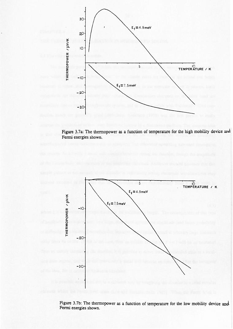
x: .... > :::1..
er w ;: o nO ~ er w :t I-
30
-10
-lO
10 TEMPERATURE I K
Figure 3.7a: The thennopower as a function of temperature for the high mobility device and Fenni energies shown.
x: .... > :::1.. .... er w ;: 0 n-o ::E er w :t I-
-10
-2.0
-30
5 10 TEMPERATURE I K
Figure 3.7b: The thennopower as a function of temperature for the low mobility device and. Fenni energies shown.

- 36-
CHAPTER 4
THE THEORY OF LOCALISATION IN DISORDERED SOLIDS.
4.1 The role of disorder in solids.
The transport properties of solids are intimately related to the wavefunctions of the elec
trons within the solid. Electrons "close" to the atomic cores for example are bound and hence
localised in space, and consequently do not contribute to the transport of heat or charge. Ionic
compounds are therefore usually poor conductors. Conduction electrons on the other hand are
essentially free to move throughout the system, and as a result solids with fractionally filled con-
duction bands are generally good conductors. Anderson (1958) was the first person to really
address the question as to how wavefunctions behave in a disordered medium. The simplest idea
is that disorder merely results in Bloch-like (if we are discussing the conduction electrons)
wavefunctions losing coherence due to scattering, but otherwise remaining extended throughout
the system. As a result, a metal will conduct however strong the disorder, though the magnitude
of the conductivity will decrease as the scattering increases. Anderson showed however that this
simple picture is not correct; if the disorder is sufficiently strong electronic wavefunctions may
become localised in the sense that their envelope decays exponentially from a given point in
space,
1'I'(r)l,ve-lr-r.ll~ (4.1)
where; is a characteristic length known as the localisation length. The consequences of this type
of localisation are remarkable. In a large, disordered system, the amplitude (and hence probability
of diffusing) of a localised wavefunction becomes exponentially small at arbitrary large distances
away from its centre. If this is the case, then an infinite system (at T = 0 ) will be an insulator!
Thus by simply increasing the disorder. it is possible to move from an extended state to a local
ised state regime, and what was previously a metal will become an insulator. After the instigator
of the idea, this is called an Anderson transition.
It is possible to think of this in a different way by imagining the disorder in a solid remains
constant whilst the Fenni level alters (Lee and Rarnakrishnan 1985). When the Fenni level is

- 37 -
low the electrons will "see" the potential fluctuations due to the disorder and may become local-
ised. When the Fenni level is high on the other hand the electrons see less of the disorder poten-
tial and so their chance of remaining extended is increased. As the Fenni level (or correspond-
ingly the electron concentration) is altered therefore, it is possible to imagine moving from an
extended (metallic) to a localised (insulator) regime, which is known as the Metal-Insulator tran-
sition. The energy which marks the boundary between localised and extended states is believed to
be sharp and is called the mobility edge Ec. This energy obviously marks the boundary between
conducting and insulating regimes. A natural question to ask then is exactly how does the con-
ductivity go to zero as the Fermi energy approaches Ep from the metallic side? Assuming that the
Boltzmann formula (equation 1.1) remains valid for £F arbitrarily close to Ec on the metallic side,
and that the lowest sensible limit for the mean free path is the interatomic separation a , suggests
that the transition is discontinuous and there that is a minimum metallic conductivity of the form.
a 3DN 1 e 2 1.. mm 3n2 T a (4.2)
There is a great deal of experimental evidence for the existence of a Metal-Insulator transition in
disordered 3D systems (see the articles by Mott et al (1975), Mott and Davies (1979), Ando et al
(1982) and Milligan et al (1985». On the other hand, careful experiments have questioned the
existence of amin, with conductivities lower than amin having been measured (see the beautiful
experiments on phosphorus doped silicon by Paalanen et al 1982, 1983). Experiments such as
these argue the case that the transition is more likely to be continuous than discontinuous. even
though it is very sharp near the mobility edge.
Although the concept of a minimum metallic conductivity is easy to understand, there are
disturbing theoretical (as well as experimental) reasons for believing it is in fact incorrect. Firstly
it assumes. without justification, that the Boltzmann formula is universally valid on the metallic
side of the transition. Secondly it assumes that localisation effects are entirely absent on the
metallic side, but are present on the insulating side leading to a divergent localisation length as
E -+ Ec. Abraharns et al (1979) proposed a scaling theory of the Metal-Insulator transition,
describing it within the language of phase transitions and critical phenomena.. which neatly

- 38-
sidestepped these problems. Near the mobility edge they argued that the only relevant length
scales are a correlation length on the metallic side and the localisation length on the insulating
side, both of which diverge as £ -+ Ec from above and below. The conclusion which is drawn from
this is that the conductivity must go to zero continuously at the mobility edge, and as a result
there is no Omin.
The scaling theory of localisation (which we shall look at shortly) highlights the importance
of the various length scales in the problem, particularly in relation to the localisation length 1;. If
the system size L is very large ( L »1; ), then the likely hood of diffusion across the sample van
ishes exponentially with L. This is known as the strongly localised regime. In the opposite limit (
L «I; ), the wavefunction is to all intents and purposes extended throughout the sample. We anti
cipate that in this weakly localised regime, the conductivity will be well described by a
Boltzmann like term plus a (size dependent) correction due to the localisation. As the system size
increases, the size dependent corrections will either decrease so that as L -+00 we recover the
metallic limit, or increase until the conductivity saturates to zero, depending upon the disorder in
the system. This implies the existence of a critical disorder, below which O-+<Js as L-+oo and
above which 0-+0 as L -+00. This critical disorder may be specified by the conductance at a length
scale of the mean free path I.
4.2 Consequences of low dimensionality.
The arguments so far have been applicable to disordered three dimensional solids. Very
quickly it also became clear that dimensionality is a crucial variable in determining the extent of
the localisation. For example. Mott and Twose (1961) were able to show quite generally that in
one dimension all the states are localised no matter how weak the disorder, due to repeated back
scattering. In the limit of weak disorder the localisation length in 10 is therefore of the order of
the mean free path (Thouless 1973). As a result, all infinite one-dimensional disordered systems
are insulators at T=O, except for very unlikely (i.e. periodic) impurity configurations. Naturally
then there is no mobility edge and no Metal-Insulator transition in one dimension. The same con
clusions have also been reached from different standpoints by Abrikosov and Rhyzkin (1978) and
- 39-
Landauer (1970). Thouless (1977) considered the case of a wire of finite cross section, and con
cluded that if its resistance R >2file 2 then the states within it would become exponentially local-
ised. The arguments he used were a precursor to the development of the scaling theory, espe-
cially in recognising that the nature of the eigenstates could be effectively described by the sys
terns resistance (or equivalently, conductance). For a resistance greater than about lOkO there-
fore, it is impossible to have metallic conduction at T = 0, and the resistance of a wire will grow
exponentially rather than linearly with its length.
The situation in two dimensions was for a long time rather unclear (scaling theory shows
that d=2 is a critical dimension for localisation). Licciardello and Thouless (1975a,b) extended
Mott's amin idea to two dimensions to predict,
a~- 0.1 e 2/t1 (4.3)
Simply on dimensional grounds there is no length scale which enters aJ!i:,., which is therefore a
universal quantity for all materials. This is the first sign that d =2 is in some sense special. Their
numerical simulations on a range of differing types of W lattice supponed the existence of this
universal minimum conductivity rather well. The situation experimentally was reviewed in detail
by Pepper (1977), who showed that this simple universality was not quite correct however. Again
we should worry about the fact that there is no a priori reason for assuming there is a region of
extended states in W. We could equally well have assumed the same in ID where it is known
that all the states are localised. The nice feature of the scaling theory is that it allows the dimen
sionality to be treated as a continuous variable and so questions such as these can be tackled. In
2D the prediction is that, in fact, all the states are localised, although the localisation length can
be very large in pure samples and diverges exponentially as the degree of disorder goes to zero.
This explains why the numerical simulations were misinterpreted, because the system sizes con-
sidered were not really large enough.
4.3 The Scaling theory of localisation.
The ideas behind the scaling theory were developed by Thouless and others (see the refer-
ences already cited). They asked the question as to what controls the behaviour of a disordered
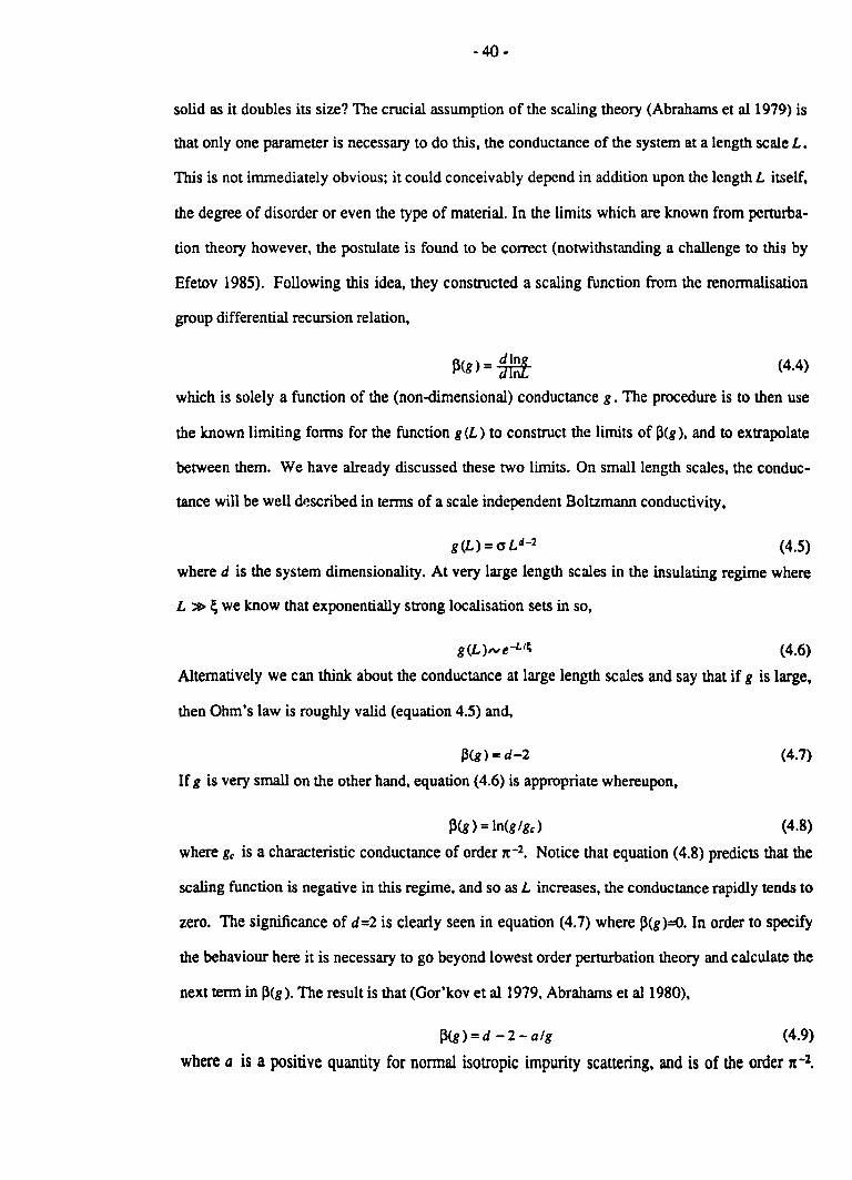
-40 -
solid as it doubles its size? The crucial assumption of the scaling theory (Abrahams et al 1979) is
that only one parameter is necessary to do this, the conductance of the system at a length scale L.
This is not immediately obvious; it could conceivably depend in addition upon the length L itself,
the degree of disorder or even the type of material. In the limits which are known from perturba-
tion theory however, the postulate is found to be correct (notwithstanding a challenge to this by
Efetov 1985). Following this idea, they constructed a scaling function from the renonnalisation
group differential recursion relation,
(4.4)
which is solely a function of the (non-dimensional) conductance g. The procedure is to then use
the known limiting fonns for the function g (L) to construct the limits of ~(g), and to extrapolate
between them. We have already discussed these two limits. On small length scales, the conduc
tance will be well described in tenns of a scale independent Boltzmann conductivity,
g(L) = (J Ld-2 (4.5)
where d is the system dimensionality. At very large length scales in the insulating regime where
L »l; we know that exponentially strong localisation sets in so,
g(L)NrL'f. (4.6)
Alternatively we can think about the conductance at large length scales and say that if g is large,
then Ohm's law is roughly valid (equation 4.5) and,
j3(g) = d-2 (4.7)
If g is very small on the other hand, equation (4.6) is appropriate whereupon,
~(g) = In(glgc) (4.8)
where gc is a characteristic conductance of order 1t-2• Notice that equation (4.8) predicts that the
scaling function is negative in this regime, and so as L increases, the conductance rapidly tends to
zero. The significance of d=2 is clearly seen in equation (4.7) where ~(g)=O. In order to specify
the behaviour here it is necessary to go beyond lowest order perturbation theory and calculate the
next tenn in j3(g). The result is that (Gor'kov et al1979, Abrahams et al1980),
j3(g)=d -2-alg (4.9)
where a is a positive quantity for nonnal isotropic impurity scattering, and is of the order n-2•

- 41 -
The scaling function is now constructed from these two limits by making the plausible assump
tions that ~(g) is both continuous and monotonic. The results are displayed graphically in figure
(4.1).
The three dimensional curve contains a point where ~(g3) is zero. This an unstable fixl:d
point from which the scaling trajectories flow outwards. Thus if g is slightly greater than g3, ~>O
and so g increases with L, eventually reaching its Boltzmann value. Conversely if g <g3, then ~<O
and so g decreases with increasing L, the system eventually becomes an insulator. The point
~(g3)=O then clearly defines the mobility edge and marks the Metal-Insulator transition. The con
ductance g3 marks the minimum metallic conductance (not conductivity) a system can have. The
assumption of continuity in the scaling function, ~,implies that there is a continuous transition as
E---+Ec and therefore that there is no minimum metallic conductivity. Furthermore, in the vicinity of
the transition we can write on the metallic side (Lee and Ramakrishnan 1985),
a",~ i;-where the correlation length l;c"" (E-£c )-V and v is a critical exponent which is universal. On the
localised side of the mobility edge we can also show that the localisation length ~ diverges
exactly as ~ with the same critical exponent. This has been verified (Paalanen 1983). Further
more, this is not restricted (in an abstract sense) to d=3. The scaling function will have a zero for
all d>2, and so there will be a Metal-insulator transition for d>2. If we write d = 2+£ and assume
£«1, then we can calculate the perturbative estimate of v, which is unity (Lee and Ramakrishnan
1985). Obviously this will not be exact for d = 3 ( £ = 1 ), and values of order 0.5 are found experi
mentally (Paalanen 1983).
Two dimensions marks the critical value of d for which ~(g) has no zero. Scaling theory
therefore predicts that there are no extended states in UJ and hence no Metal-Insulator transition.
As the system size increases, eventually the conductance will tend to zero and the sample will
become an insulator. For pure systems this only becomes apparent at truly large length scales,
since when g is large, ~(g) is very small. For many UJ systems of interest we can therefore
expect L«~, whereupon traditional transport theory will provide reasonable answers. The
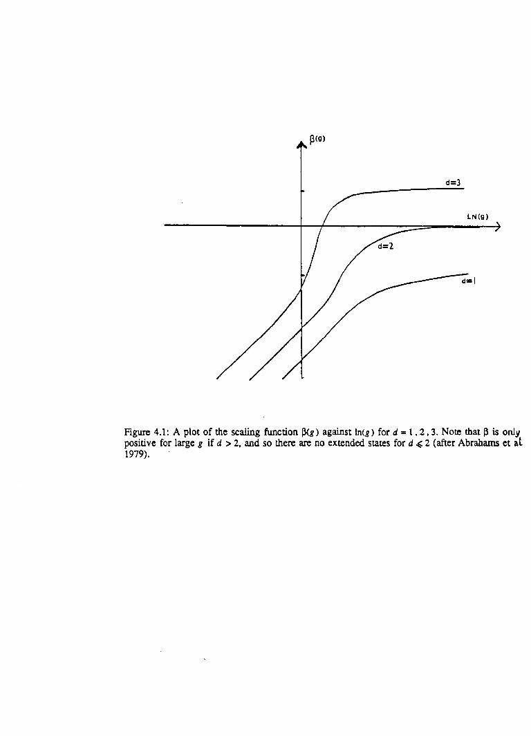
d=]
Figure 4.1: A plot of the scaling function ~(g) against In(g) for d = 1 ,2,3. Note that ~ is onl'y positive for large g if d > 2, and so there are no extended states for d ~ 2 (after Abrahams et at 1979).

- 42-
prediction for one dimension however is that as L increases the conductance rapidly tends to
zero. This case will be further discussed in section (4.6). For now we note that scaling theory cer-
tainly supports the results of Mott and Twose (1961) and Landauer (1970) that there are no
extended states in pure ID and no metallic regime.
4.4 The weak localisation regime.
The scaling theory of localisation gives us a prescription for the behaviour of the conduc
tance at zero temperature of a disordered solid, and leads to concrete predictions such as the
existence of certain universal exponents near the mobility edge. In the weakly localised regime
we can say a great deal more because the traditional methods of diagrammatic perturbation theory
are still valid. In the strongly localised regime, transport at finite temperature occurs via hopping
which is calculated in a different manner, by using rate equations, percolation theory and the
theory of random walks. For reviews of this regime see Butcher (1976), Shklovskii and Efros
(1984). We should also mention in passing that attempts have been made to treat the transition
(from the weak to strong localisation) within one theory, using self-consistent perturbation
methods (Vollhardt and Wolfle 1980) It is not clear however how to reconcile all of the
difficulties which arise when taking this approach.
A helpful picture to consider when thinking about the weakly localised regime ( kF I» 1 ) is
to think of the electrons executing random walks from impurity to impurity· with a mean step I
(Al'tshuler and Aronov 1985). Imagine an ensemble of impurities in real space and ask what is
the probability for an electron to diffuse in this manner from a point A to another point B (see
figure 4.2)1 If we sum the amplitudes for all possible paths, then the probability is simply the
square modulus of this quantity,
Prob. = Il:As 12 (4.10) s
which may be written as,
(4.11)
The first term is simply the classical sum of all the probabilities to travel along any path. The
second term represents an interference of all the various amplitudes which when averaged over a
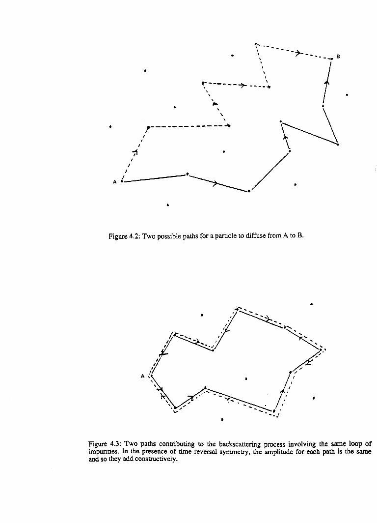
•
•
• "-, --, ----;t>-
\ --- __ B , \
\ \ -- \ .. -----~ ----~ , , , .,.. . /..------------\ ON
A !_'--/~------.~./O ° •
Figure 4.2: Two possible paths for a particle to diffuse from A to B.
• '-. / .. ~' ........... , ...
I ...
I .' ... ,~, , I· ........... I "
• ,
........ , I
...... J •
"
Figure 4.3: Two paths contributing to the backscattering process involving the same loop of impurities. In the presence of time reversal symmetry, the amplitude for each path is the same and so they add constructively.

-43 -
large number of paths. will usually be zero. This is the assumption that Boltzmann theory makes.
There is however one very imponant case where this need not necessarily be true. Consider the
probability for a particle to return to its initial starting point (figure 4.3). and in particular. con
sider the two paths shown where the amplitudes A I and A 1 correspond to a passage around a
closed loop of impurities but in opposite senses. In this case. A I and A 1 interfere constructively so
we must write.
IAI+A111= IA111+ IAlI2+2ReA1Ai _4IA\12 (4.12)
The classical result neglects the interference term and so predicts the probability of return is
21A 112. Providing we can show they have a finite weight. inclusion of these interference terms
will therefore mean there is a greater possibility of returning to the starting point (backscattering)
and so the resistance of a sample will increase. This physical picture emphasizes the quantum
nature of the localisation phenomenon. which leads to a negative correction term to the
Boltzmann conductivity.
When we expanded the S-matrix to calculate the conductivity (equation 3.14) an infinite
number of diagrams were produced. One subset gave rise to the Boltzmann result. We anticipate
that another subset will represent the leading correction to aB and will have its origins in weak
localisation. These diagrams are the maximally crossed diagrams. first discussed in a different
context by Langer and Neal (1966), Neal (1967) and in detail by Gor'kov et al (1979) and Abra-
hams et al (1980), /( /(' /( /(./(, /(' k /(./(, k· K2 k'
i ~ , '> , < ,) , , , ,
'*X* I
~* ~ , I , , . ,
+ " ... 'J.: it ••• " ,., , ... , ... , ... , I , ,
I ,
I • , ... .' , I , ...
oC , . (' "
/( /(, /( /(' ok, /(' K /(' -k 2 k'-/(, /('
They account for precisely the kind of interference terms we have just been considering, but
represented in momentum rather than real space (Bergmann 1983). A customary redrawing is to
reverse the lower line which gives the ladder diagrams in the particle-particle channel (known as
the Cooperon).

- 44-
k k' if 1<+1<, k' k k+It, k+k2 If'
i ') ) , "
i I , I , I
1< ~ ';I( ~ ~ )( 0 ... ... 00
0 , ) > )'
/(, It k' k' -k, k k' Jr' -It, It' -It 2 k
Each diagram is of the same order so the entire series has to be summed. For zero-range scatter
ers, the diagrams fonn a geometric series and so the summation is trivial. The interesting thing is
that the sum diverges for small Q .co*'( where Q = k+k' ) like (DQ 2 - i (0)-'. D is the diffusion con-
stant =v; T./d. This strong correlation between states of opposite momenta is the signature of
localisation; naively if one wanted to make a localised wavepacket, one would add together plane
waves of opposite momenta to make standing waves. This idea that correlation between states of
opposite momenta is responsible for localisation incidently disagrees with the model of Kaveh
and Mott (1981), and Berggren (1982a),b» which is now (for this reason) believed to be incorrect
(Davies 1987, private communication).
The divergence arises because in an infinite system there are arbitrarily many loops which
can contribute to the backscattering process. In a finite system however the maximum loop size I~
of the order of the system size L, which introduces a lower cut-off in the Q - summation of order
lIL. The correction to the conductivity is then (for ro=O),
(4.13)
where the upper Q cut-off is 11/. Notice that the correction term is both negative and size depen-
dent. In 3D.m and ID this predicts (assuming that L »1 ),
e 2 t 1 030 = OB - 1IftJ (T - r) (4.14a)
e2 . aw ... 08 - 1i ltZ In(Ul) (4.14b)
t 1 aID = a8 - u L (4.14c)
The weak localisation correction depends only upon simple constants and so is the same for all
materials, whether they are semiconductors or metals. This agrees with the predictions of scaling
theory. As the length scale L increases, the 3D conductivity saturates to i1 length independent
-00 refers to the frequency of the external applied field.
- 45-
constant as we anticipated would happen above the Metal-Insulator transition. In ID and ID, the
weak localisation tenn grows until it dominates the Boltzmann tenn (at which point perturbation
theory breaks down). From the length scale at which aWL =aB we can deduce the approximate
size of the localisation length. We find that in ID ~ = iexp(7tk,1I2) (so if k,l is large then the
localisation length is also). whilst in ID. ~Ioc = ru. and all states are localised on a length scale of
the mean free path (Thouless 1973).
So far the discussion has been restricted to zero temperature. Before discussing finite tem
perature. recall the nature of the singularity in the Cooperon at finite frequencies. Had we retained
ro, then the length scale LO) = (D Iro)Ya would have provided a natural cut-off in the Q - summation,
and would (if LIJ)<.L ) have replaced L in the above fonnulae (equation 4.14a),b),c». This is
extremely significant for it is saying that finite frequencies can cut-off the weak localisation
phenomenon (Gor'kov et al 1979, Al'tshuler et al 1982). If the loop size (figure 4.3) is greater
than LIJ)t the A.C. field destroys the phase coherence needed for localisation and so provides the
length scale which determines the magnitude of the weak localisation tenn. To introduce finite
temperatures, we make an analogy with the above and note that inelastic scattering will also des
troy the phase coherence necessary for localisation. If the inelastic effects are characterised by a
time ~, the length scale L~ = (D ~)Ya will then be the length scale which replaces L. Thouless
(1977) interpreted the time 'tQ as the lifetime of an eigenstate of the disordered system. Al'tshuler
et al (1982) however pointed out the fact that the significant timescale is the time over which
phase coherence is lost, and called 't, the phase relaxation time. The phase relaxation time need
not be the same as the the inelastic time.
The phase relaxation time 't, is temperature dependent, and at low temperatures is con
trolled by electron-electron scattering. When low momentum transfers are important, the phase
relaxation time is the same as the electron-electron scattering time, which in disordered systems
varies as T-4/2 (Schmid 1974). When low energy transfers are important, the relevant process is
equivalent to the interaction of an electron with fluctuating electromagnetic fields, the so called
Nyquist mechanism. The temperature dependence of't. in this case goes as T'}j(d~) (Al'tshuler et
al 1981, 1982). The sensitivity of the weak localisation tenn means that it controls the
- 46-
temperature dependence of the conductivity, since at low temperatures, GB is essentially indepen
dent of T. As the temperature drops, so inelastic effects become less important, causing the weak
localisation correction to G to increase and the resistance to increase. In 2D the prediction is that
there will be a In(T) correction to the resistance. This was first observed by Dolan and Osheroff
(1979) and has been reproduced many times (see the reviews by Bergmann 1984, Lee and
Ramakrishnan 1985). In one dimensional wires it is more difficult to interpret the data, though
there are now reports of the observation of the Nyquist mechanism. with a T-li3 dependence found
in the length L. (Thornton et al 1986, Lin and Giordano 1987).
4.5 Magnetic fields and interaction effects.
The inherent instability of the Cooper channel to perturbations which destroy phase coher
ence (violate time reversal symmetry) means many other effects can introduce new length scales
into the problem. In the presence of a magnetic field, the change of phase gained by going around
a loop of impurities depends upon the sense in which the loop is traversed. As a result, the rela
tive phase upon recombination depends upon the loop size and so on average, magnetic fields will
destroy localisation, and lead to negative magnetoresistance. The theory was first worked out for
3D systems by Kawabata (1980,1981), and for 2D systems in a perpendicular field by Al'tshuler
et al (1980). The extension to longitudinal fields in a 2D system of width a, as well as cylindrical
wires with either field orientation was made by Al'tshuler and Aronov (1981). The behaviour
found in these cases depends subtly on the relative magnitudes of the magnetic length LH ,L.
and the channel width a. Experimental results are in good agreement (for example Newson and
Pepper 1985, Newson et al 1985, Thornton et al 1986, Lin and Giordano 1987). Magnetic fields
can also lead to very interesting effects in multiply connected structures, with both oscillations in
~ (the flux quantum) and ~2 being predicted and observed (Al'tshuler et al 1981, Sharvin and
Sharvin 1981, Datta and Bandyopadhyay 1987, Dolan et al1986, Washburn et alI987). Many of
the relevant experiments are described in the recent review by Aronov and Sharvin (1987).
Spin-orbit scattering defines a new timescale '(.0 and a new length scale Lso. Hikami et al
(1980) considered the behaviour of a system at finite temperature and magnetic field, when spin-

- 47-
orbit scattering is present. The magnetoresistance can now have quite exotic behaviour and may
be both positive and negative. The spin-orbit effect is greatest in metals, and the theory has been
confirmed to quite remarkable accuracy (Bergmann 1982, Santhanam et al 1984, Licini et al
1985, Lin and Giordano 1987). Another mechanism which can produce similar effects is spin-flip
scattering due to magnetic impurities (Bergmann 1984).
So far we have said little about electron-electron interactions. In addition to localisation,
which is a single particle phenomenon, interaction effects have also been studied extensively in
disordered solids. In the strongly localised regime, the theory is usually developed in terms of
various parameters (such as the Hubbard U ) which characterise the electron-electron repulsion
term. It is believed that interaction effects can produce a similar effect to the Metal-Insulator tran
sition (the Mott transition) by opening up a gap in the density of states at the Fermi level (the
coulomb gap). For detailed reviews of these and other phenomena in the strongly disordered
regime see the reviews by Pollak and Ortuno 1985 and Efros and Shklovskii 1985. In the weakly
localised regime, more is known qualitatively because diagrammatic perturbation theory is appli
cable. The important point is that because the electron motion is diffusive rather than ballistic,
the electron-electron interaction is generally enhanced. It is known for example that interactions
lead to a loT term in the conductivity in 2D, exactly as the localisation term does. It is also
known that interaction effects are much less sensitive to weak magnetic fields than localisation
effects are, and so it is possible to distinguish the two contributions by suppressing the weak
localisation term in a magnetic field. To a first approximation, the two effects are additive. It is
only because of this that it makes sense to talk of the localisation problem in isolation. Excellent
reviews of interaction effects in the weakly disordered regime have been given by Al'tshuler and
Aronov 1985, Fukuyama 1985 and Lee and Ramakrishnan 1985.
4.6 Tbe one and quasi-one-dimensional regime.
As we have been interested in systems which are inherently one dimensional we shall study
this regime in a little more detail. This will highlight some of the important ideas we wish to
return to later in this work. Since Mott and Twose (1961), further investigations have proceeded

-48 -
along two distinct paths. The first route has relied on the Green's function methods; essentially
solving a kinetic equation. Berezinskii (1973) considered the disorder to all orders to prove that
all the states in one dimension are indeed . localised. This view was also supported by Abriko-
sov and Rhyzkin (1978). For wires in the weak localisation regime, AI'tshuler and Aronov (1985)
argued that the corrections to the conductance will be strictly one dimensional if the width of the
wire is less than the relevant length scale, otherwise they will be two or three dimensional
depending on the geometry. In the absence of magnetic fields they suggested that the relevant
length scale is the phase breaking length L •. They also considered finite length effects (AI'tshuler
and Aronov 1984) and showed that for very short wires (L,..,L.) boundary effects in the longitu-
dinal direction are also important This idea has been developed by Santhanam (1987), and the
effect has been observed experimentally by Masden and Giordano (1984).
The second approach to the problem has utilised the Landauer formula (1970), or variations
of it. Landauer expressed the conductance of a one-dimensional system in terms of the transmis-
sion probability T for an incident particle to per,etrate a length L ,
(4.15)
and showed that the ensemble average <G > 00( e-LI~. Clearly this implies localisation of the states
as L-+-. The derivation of equation (4.16) is sufficiently simple to make it an attractive method
for studying transport in disordered solids. (A word of warning; although the derivation is simple
it is also subtle. and attempts to generalise the result to higher dimensions lead to controversy for
a number of years. This has now been satisfactorily resolved; for a chronological development of
the problem see Landauer 1970, Economou and Soukoulis 1981. Fisher and Lee 1981. Langreth
and Abrahams 1981. Thouless 1981, Economou and Soukoulis 1981. Buttiker et al1985. Eranen
and Sinkkonen 1987). A most important point is that the Landauer formula can be applied to a
single sample rather than representing some kind of ensemble average. This has revealed a whole
range of new phenomena in small systems which are not seen after averaging has taken place. In
the strongly localised regime, the conductance is a violently fluctuating function of Fermi energy
in ID (Azbel and Soven 1983. Lee 1984. Mclnnes and Butcher 1985). For a given Fermi energy.
- 49-
the conductance will also vary enormously from sample to sample, and as a result <G> is not a
statistically well defined quantity. This reflects the fact that the mean conductance is very dif
ferent to the typical conductance in ID. Anderson et al (1980) used the Landauer formula to show
that In(1+g-1) is the well defined scaling variable in that it has additive mean. This idea was pur
sued in a second paper by Anderson (1981) and a heuristic generalisation to higher dimensions
given. Using these higher dimensional type expressions, the conductance of finite cross-sectional
wires has been discussed by Azbel (1980a.b, 1981), small rings by Buttiker et al (1985) and even
device characteristics have been calculated (see e.g. Davies 1987). The Landauer formula is ideal
for performing numerical calculations of this type. On the other hand it is not so easy to extract
analytical results, and the extension to finite temperatures is not trivial. Nevertheless it seems that
the Landauer expressions are becoming more widely used in studying small systems, especially
when the scattering is small or even non-existent (Van Wees et al 1988).
4.7 Fluctuation phenomena.
The Landauer picture tells us that the conductance of small samples is sample dependenL
Experiments in ring geometries and in wires have revealed such sample dependent features as a
function of magnetic field (Umbach et al 1984) and chemical potential (Kaplan and Hartstein
1986). The important feature of these fluctuations is that they are reproducible in a given device
and of universal amplitude at T=O. The samples they are observed in are metallic ( L »~ ) and are
called mesoscopic, meaning somewhere between macroscopic and microscopic. The fluctuations
in mesoscopic devices (Universal Conductance fluctuations) are now relatively well understood
(Al'tshuler 1985, Lee and Stone 1986, Al'tshuler and Khmel'nitskii 1986, Lee et alI987).
The Kubo formula. in principle, gives us the conductance of a specific sample with a
specific impurity configuration. In practice this is too difficult to evaluate which is why an ensem
ble average is taken. In order to study sample specific fluctuations therefore. we need a way of
getting around this problem. Lee and Stone (1985) hypothesised that the fluctuations in the con
ductance of a given sample as a function of Fermi energy or magnetic field could be viewed as
the statistical fluctuations which would occur in an ensemble of samples differing only in their

- 50-
microscopic impurity configurations. This enabled ensemble averaging and standard techniques
to be reintroduced into the problem. In particular, they considered the correlation function,
F(£p, &. B. AB) = <g (£F. B) g(£F+&. B+AB» - <g (£F, B»<g(£F+&.B +AB» (4.16)
where < .... > denotes ensemble averaging over many samples. When & = MJ = 0, F is simply the
variance of the conductance amongst the ensemble of samples for a given £F, B. The assumption
of the ergodic hypothesis is that this is representative of the magnitude of the fluctuations in a
given sample. In the other limit where ~£ and MJ are large, the conductances will be uncorrelated
and F will be zero. The decay lengths Ec. Bc of F will then be representative of the mean spacing
between the fluctuation peaks. The correlation function has been evaluated diagrammatically
(Lee et al 1987) and the main results are as follows. The amplitude of the fluctuations in £F or B
is independent of the size of the sample and only weakly dependent upon its shape. Furthennore,
this amplitude is universal and of order e2/h at T=O. The spacing between the peaks in energy is
given by,
Ec =1f1t2DILl (4.17)
which just relates to the time for the electrons to diffuse the length of the sample in the current
carrying direction (Thouless 1977). The corresponding expression for Bc is a little more compli
cated since it depends upon the orientation of the field (Lee et al 1987). We shall find later that
similar ideas can be found for the thennal transport coefficients, which also show fluctuations in
mesoscopic devices. The important point to stress is that the origin of these fluctuations is quan-
turn mechanical and not classical. To see this, imagine forming a large conductance by the adding
together of smaller conductances which are essentially randomly distributed. Classically the vari-
ance of the total conductance is given by the central limit theorem,
(4.18)
and since < G > ... L d - 2. this predicts that var (G),.., L d - 4. In all dimensions less than d = 4 the
conductance therefore self-averages classically. In the present problem however the variance is
independent of system size; the quantum mechanical origin of the fluctuations exactly cancels the
classical self-averaging behaviour and the fluctuations persist out to all length scales. This is true
for T = O. At finite temperatures however there are two important length scales which enter the

- 51 -
problem and lead to averaging effects. Firstly the work on weak localisation has shown that a sys
tem is quantum mechanical up to a length scale L. whereupon classical combination rules are
appropriate. At length scales greater than L. we can therefore sub-divide our sample into regions
of size L. which are then added classically to give,
var G(L,T) =var G(L =L., T) [ ¥-r (4.19)
As the sample size exceeds the phase breaking length, the fluctuations therefore begin to self
average, and die away completely in the thermodynamic limit. The other important length scale is
the thermal diffusion length LT = (hDlkT)v-. which determines energy averaging (thermal broaden-
ing) in the sub-regions defined on a length scale L .. In particular if LT «L. the fluctuations will
have been essentially averaged out even at a length scale Lr = L., because in this case ks T » Ec.
What we are then left with is the average behaviour such as weak localisation. Experiments to
look for fluctuations must therefore be performed at suitably low temperatures where the system
size is much less than either of these lengths. A very detailed account of all finite temperature
effects has been given by Lee et al (1987), and recent reviews have been given by Lee 1987,
Al'tshuler 1987 and Webb et al1987.

- 52-
CHAPTERS
WEAK LOCALISATION IN THE QUASI-ONE-DIMENSIONAL REGIME.
5.1 Introduction to the problem.
In the previous chapter, a general overview of localisation and in particular weak localisa-
tion was given. We now wish to perform a calculation of the weak localisation term in a quasi-
one-dimensional system explicitly retaining the sub-band picture to account for finite width
effects. This will accomplish two things. Firstly the results will be expressed in terms of an aniso-
tropic diffusion constant, with differing longitudinal and transverse components. Secondly, since
the results are valid for an arbitrary number of occupied sub-bands, and hence arbitrary channel
width, it enables an explicit calculation of the dimensional crossover from a ID to a ID scaling.
This is particularly interesting since many experiments can now probe such a transition. The role
the sub-bands play in determining the weak localisation correction turns out to be rather different
from their role in determining the Boltzmann term.
Most of the work that has been carried out on weak localisation has assumed an isotropic
diffusion constanL Anisotropy can arise in many ways however so it important to understand how
this affects the results. The simplest way it can happen is if the effective mass is anisotropic, as in
silicon for example. This case was considered by Wolfie and Bhatt (1984), who found that the
effect of the anisotropy can be completely absorbed into an anisotropic diffusion constant,
00 = - 2e 2 D 0 ~ t 1111 n:II 1111 t -i co + t D~11 q J
11
(5.1)
We shall find a similar result holds when the anisotropy is due to finite width effects (sub-bands).
and shall derive analytic expressions for the D~ for this case. The correction term always has
the same anisotropy as the Boltzmann term. The consequences of equation (5.1) have been inves-
tigated experimentally and found to be correct (Bishop et al1984).
When sub-bands were discussed earlier, a general feature was the lack of translational sym
metry in the confined directions leading to Green's functions non-diagonal in the sub-band
indices. The problem was simplified by assuming that the sub-bands were sufficiently far apan

- 53-
for the off-diagonal elements to be small. If on the other hand we want to demonstrate a ID to a
2D crossover where near the 2D limit the sub-bands are necessarily almost degenerate. this
approximation is no longer good enough. In order to proceed we shall therefore use a slightly dif
ferent model which assumes periodic boundary conditions in all directions (Fisher and Lee 1981,
Cantrell and Butcher 1985). The repeat symmetry in the confined directions produces a Green's
function which is diagonal in the sub-band labels without recourse to approximation once the
ensemble average is taken. The choice of such a model is not expected to affect the essential phy-
sics in the problem (a point we shall return to) and is certainly sufficient for illustrative purposes.
For a non-interacting electron gas confined to a region ( L xW ) the wavefunctions in this model
are,
'" _ 1 ik;C w yaA: - (LW)"" e e (5.2)
where k is taken to be continuous and,
ko. = 2na I W (a = O.±1.±2, ... )
a thus plays the role of a sub-band index, and the unpenurbed sub-band origins are simply
(2n:1W)2 a2/(2m). (In the interests of conciseness, we set 1(=1 and m· =rn, and restore the full depen
dences at the end of the calculation). The thickness in the third dimension will be taken to be
sufficiently small that the electrons are always in the ground sub-band associated with
confinement in that direction. Consequently it can be ignored altogether without loss of general-
ity. This situation is relevant to pinched MOSFETS for example. When the width W is small, the
ko. are discrete and represent the different sub-bands. In the opposite limit, the ka are quasi-
continuous and the wavefunction is simply a 2D plane wave. This simple crossover in the
wave function will reflect the crossover in the transpon coefficients we wish to explore.
5.2 The single-particle self-energy.
The same model for the impurities will be used as in previous chapters. Within the present
model the matrix elements (squared) are simple constants. and so the self-energy is only a func-
tion of the energy variable E. In order to ensure the correct divergence in the Cooperon (which is
responsible for the weak localisation behaviour and guaranteed in the presence of time reversal
- 54-
symmetry), it is important that the self-energy is treated consistently with the approximations
made in evaluating the current-current correlation function. The divergence arises as a result of a
delicate cancellation between these one and two particle properties. We will show that the self-
consistent Born approximation considered earlier is appropriate. Again we will ignore the real
part of the self-energy. (Retaining the real part throughout leads to the same divergence in the
Cooperon and only alters the single-particle properties). If - ne) is the imaginary part of the
retarded self -energy then,
- ne) = Im [ '1fJ J It, (£+~-q 2/2m -k i /2m +i ne)r1 (5.3)
which, since r is independent of momentum or sub-band labels is equivalent to saying,
(5.4)
lIP: where GR.A are the retarded and advanced Green's functions respectively. As well as determining
r this equation provides a consistency requirement which must be maintained throughout the cal-
culation. Since q is a quasi-continuous, one-dimensional variable, the sum over q may be per-
fonned by a contour integral. with the result that,
(5.5)
where the identity,
(a +ib)=(2m(e~)-ki+i2mn',\ b>O (5.6)
defines a and b. As it stands. equation (5.6) is still a complicated expression for r since a and b
depend upon r themselves. and in general must be solved numerically. The density of states in
this model is linearly related to r.
gee) = 2Lwr njU3n
(5.7)
and when the sub-bands are well separated. will show structure similar to that discussed previ-
ously (figure 3.2).
The various limiting behaviours of r serve as a demonstration of dimensional crossover in
multi-sub-band transport. The separation of the sub-bands is controlled by the system width W •
If W is sufficiently narrow so that the broadening is less than the sub-band separation energy.

- 55 -
then the sub-band concept is meaningful and they are well defined. As the width of the channel
increases, so the sub-band separation decreases (as lIW2 ) and eventually r will be of the order of
this spacing. At this point, the concept of sub-bands becomes meaningless and the self-energy
rapidly approaches its two-dimensional limit As an order of magnitude estimate of this effect,
suppose the system is in the 2D limit where r IX nj Uo2m. As we decrease the width W, r will stay
roughly at this value until the sub-band spacing is of same order. If the Fermi energy at this point
lies between the nth and (n +l)th sub-bands this is equivalent to saying,
2 2 2 -K241t2 r2D~njUom=[(n+l) -n] 2m'Wz
Now since kFal21t111W, this implies,
W2 - 41tWl - 4n21lkF = 0
where I is the 2D mea., free path =1f2kFI2mr. In the weakly disordered regime where the theory
is applicable, kF I» 1 and so W =' 47tl. This is an important result. It states that if we define a nar-
row channel in a WEG, then the sub-band structure only becomes apparent for widths less than
the mean free path in the 2DEG . At length scales smaller than this the density of states will begin
to show structure and the possibility of observing QSE becomes realistic. At greater length scales
the density of states is simply a constant, exactly what we would expect of the 2D limit Although
this calculation has been performed for quadratically spaced sub-bands, we expect that the essen-
tial result (that the relevant length scale is the mean free path) is the correct one for the density of
states, even if the sub-bands are linearly separated in energy for example.
5.3 The weakly localised conductance.
Within this new model, we proceed in the usual fashion and expand the current-current
correlation function using the S - matrix. In the previous chapter we saw that the relevant quantity
to discuss is the conductance rather than the conductivity, and so even though the difference is
trivial in this limit we shall refer to conductances from now on. The Boltzmann term we associate
with the simple bubble diagram,

- 56-
In chapter 3 this diagram was evaluated in detail (equation (3.21)). Performing the sum over k by
a contour integral gives (at T=O ),
e l a J GB = 1ii1iTr t (al + b l ) (5.8)
where a and b are defined through equation (5.6) and evaluated at £=0. This expression is the zero
temperature Boltzmann conductance for an arbitrary number of occupied sub-bands. When the
sub-bands are well separated in energy this will show oscillations as a function of Fermi level,
which is simply the manifestation of the quantum size effects discussed in detail in chapter 3.
When the channel width is wide, the sub-bands mix together and GB tends to its 2D limit The
criterion for this to happen is exactly the same as for the self-energy and the density of states,
namely that the channel width should be of the order of the mean free path. Above that the
Boltzmann conductance will appear two-dimensional and no QSE are to be expected. Experi-
ments to resolve QSE must therefore take place in sufficiently narrow channels of course.
The weak. localisation term is associated with the maximally crossed diagrams. which when
drawn in the particle-particle channel look like, Ol • IX, 0.0, (X. (X 2
(X If Ol'If' rxlf 1f.1f, c.' If' olf If-If, /( - /(2 ex'/('
I ) ~ ; I)' » I
, , , :+.'**
, I
* * ~ • I ' ... )' of- ' , ' +' ••• I '
;r, , , , , ~ I '\. , , I . , , , I , . • , ,
" I ... , ,
'(' ,
c >
ex/( (X'If' Ol/( (x' - ex, a'lf' ex If 0'.02 (X' .(X, a'/('
k' .k, k'·k, k'-k,
We use the notation Q=k+k' and analogously K=kll+k~. As usual. the choice of &- function
scanering potentials enables the series to be summed as a geometrically. The important contribu
tion to the weak localisation comes from the terms where the Green's functions have the opposite

- 57-
analyticity i.e. when the upper line is retarded and the lower advanced. Retaining these tenns then
gives,
llGWL =- ~~L2 j de ~. k(-k+Q) GR(k.ka,e) GA(k.ka.£) S(Q.K.e) -- t .t:t!.K
xGR(-k+Q.-ka+K.£) GA(-k+Q.-ka+K.£) ¥ (5.9)
The scattering vertex may be written in the simple closed form,
where ro = nj uilWL and,
ro S (Q .K ,E) = 1 - tOR
R = ~ GR(q.kp.£+ioo) GA (-q+Q ,-kp+K,£) tt,
(5.10)
(5.11)
We have retained the finite frequency component 00 in the scattering vertex as a guide to how the
phase relaxation time will enter the problem. Equation (5.9) is the full expression for the weakly
localised correction to the Boltzmann conductance. Notice that it contains the factor at lde which
is responsible for thermal broadening. Thermal broadening is usually considered unimportant in
the theory of weak localisation, but in sub-band systems may lead to sizeable effects, and its
importance in certain regimes will be discussed in a little while.
In the limit Q ,K ,CJ>-+O the scattering venex diverges (compare the denominator of equation
(5.10) with the R.H.S. of equation (5.4) which is identically zero). This divergence arises because
we have been careful in maintaining self -consistency between the two particle correlation func-
tion and the single particle self -energy. Since the small Q.K.oo terms are therefore going to be the
most important, it is admissible to work only to lowest order in these quantities. which means we
can neglect all Q ,K dependence except that arising in the scattering venex. To begin with we
shall work at T=O. The sum over k in equation (5.9) may be performed by a contour integral
(with two double poles in the upper half plane) with the result,
(5.12)
where a and b are defined as before. Next we perform the sum over q in equation (5.11) for R,
again by a contour integral (but with only two single poles in the upper half plane). The answer is
rather complicated, however since we are only interested in small values of its arguments we can

- 58-
expand to lowest order to give,
(5.13)
In order to facilitate the derivation one makes use of the symmetry properties of the original
expression. The leading term of ro R is unity (c.f. equation 5.6) ensuring the correct divergence
in the Cooper channel. To this order, S may be written,
(5.14)
where D and Dp are defined by,
niUJ a3
D = 2Wmf2 ~ (a4bZ) (5.1 Sa)
D _ njUJ k[a 5
p - 2Wm f"l ~ (a 2+b 2)J (S.ISb)
Notice that exactly the same combination of factors occurs in equation (5.15a) for D as in the first
factor of equation (5.12 ) for llGwL. The net result is that we can write,
2e 2D I llGwL = -1tJ:I"" b DQ 2 + Dp Kl_; CJ)
(5.16)
Compare the above result with the result of Woltle and Bhan (1984) (equation 5.1). The
two results are identical and so we identify D and Dp with the longitudinal and transverse diffu
sion coefficients in a multi-sub-band system. The anisotropy in the present case is not due 10 an
anisotropic effective mass but due to finite width effects. Let us consider the form of these diffu-
sion constants a little more closely. Suppose the sub-bands are well separated and that all the
electrons are confined to lowest sub-band. It is easy to show in that in this case
r c!. nj U a IWkF ,a '::! kF and b et 0 whereupon D = k; tlm 2 and Dp = O. Thus in this limit we have the
usuallD {\iffusion down the channel and almost no diffusion across it In the opposite limit wht!n
W is in excess of the 2D mean free path so that many sub-bands are occupied, we can replace the
sum over kp by an integral to evaluate the diffusion coefficients. This is rather trivial and gives us
the result that we would expect, namely that both D and Dp tend to the 2D result (V tl2ml) and
we regain the isotropic situation. Thus our interpretation of these constants as describing the diffu-
sion in a multi-sub-band channel is very plausible. As further evidence, it should be noted that D

- 59 -
is related exactly to the Boltzmann conductance (equation 5.8) and the density of states (equation
5.7), via the usual Einstein relation.
S.4 The one dimensional limit for llGwL.
The expression we have derived for the weak localisation correction to the conductance is
valid as long as the expansion in Q, K is valid. This implies that the terms in equation (5.13)
involving Q and K should both be less than unity for all values of k~. There are three regimes to
consider, when Ik~1 «kF ,lk~1 »kF and Ik~1 =kF, and we want to ensure that Q<2mrta and
K <2m rca'4b2)/(k~ a4). The results are presented in tabular form below:
REGIME VALUE OF a CONSTRAINT ON Q CONSTRAINT ON K
IKnl « K f ad kf Q<2mr/Kf K <2mr/Kn
IKnl » Kf ac! mr/Kn Q<2Kn K <K~/mr
"'" 1Knl::ll Kf ac:!(mr) Q < 2{mr) 11",
K<4mr/Kf
All these conditions are satisfied if Q and K are both resuicted to be less than 2m rtkF, which then
constitutes an upper cut-off to the Q, K summation. This quantity is simply lIJ where I is the
elastic scanering length at the Fenni surface. This is the same criterion as used in conventional
treaunents for the upper cut-off. which is not that surprising as I represents the smallest loop size
(figure 4.3) that can yield the interference necessary for weak localisation.
To begin with we shall consider only the K=D term. In the standard fashion inelastic effects
are introduced by replacing i w by 1I't~ where 't~ is the phase relaxation time at the Fermi level.
Replacing the sum over Q by an integral we can easily derive (reinserting fi),
G 2el IL~ II WL =- ~L~tan- T (5.17)
where L~ = (D't~)1'J and I C/.(D 't) .... Since at low temperatures L~» I we finally obtain,
(5.18)
This is the exact one dimensional result Thus in situations where the K = 0 term dominates.
regardless of the number of occupied sub-bands, the weak localisation scaling will be linear in L.,
-60 -
and all the infonnation about the sub-bands is contained in L .. A simple qualitative insight into
this is provided by recognising that weak localisation is a quantum interference phenomenon.
K = 0 implies an interference between states in "opposite" sub-bands (i.e. ka. and -ka) which (in
this model) in some sense corresponds to transverse standing waves. The resulting contribution
thus arises solely from motion along the strip and appears one-dimensional. Notice that the length
L. depends upon the longitudinal diffusion constant. This is the length scale which enters the for
mula for the conductivity. The length scale which controls the dimensionality of the correction
term on the other hand is slightly different, which we shall now explore.
5.5 The intermediate regime and the ID crossover.
We have just shown that the K = 0 term is responsible for the weak localisation term behav-
ing one-dimensionally. The question we need to answer therefore is when is this term dominant?
Firstly we note that the expansion employed to derive equation (5.16) was only valid for K < 111
and that K=21t11IW. If W<I this can only be satisfied by K=O. This then is the first important
result; if the width of the channel is less than the elastic scattering length then the weak localisa
tion correction should appear one-dimensional. From equation (5.16), if W> I the K = 0 term will
still continue to dominate provided,
or,
(5.19)
The first remark about this is if the diffusion constant is isotropic (Le. Dp = D ) the condition for
ID behaviour is that W <L. (the factor of 2n is not that important to our discussion). This was the
case considered by Al'tshuler and Aronov (1981) and the result they obtained. We have seen that
D, and D are essentially equal to each other when the channel is very wide, and so this criterion
is valid in this limit (the so called dirty channel case). If on the other hand W and hence the
number of occupied sub-bands is small, then the full condition above should be used. We can
analyse this in a slightly different way by remembering that L.=(D t.)1o'o so,

- 61 -
W < 21t(Dp 't~)'n = L" (5.20)
The length scale L" is a transverse inelastic length involving the transverse diffusion constant but
the same phase relaxation time as in L .. These two length scales are than related by
L"IL. = (DplD )'n. This transverse length is the length scale which controls the system dimen
sionality as far as weak localisation is concerned, and is our second important result Combining
the two, we predict that the weak localisation in a multi-sub-band wire will scale one-
dimensionally if,
W < MAX (L" , l) (5.21)
We will discuss the implication for experiment in a moment. The physical significance of the
length scale L" is rather clear, it is simply the distance an electron can diffuse across the channel
before suffering a phase destroying scattering event. If W is less than this length, then the elec-
trons can "sense" the confinement which in turn leads to a one-dimensional correction term. We
should stress that the distinction between the transverse and phase breaking lengths should be
made for any source of anisotropy, and so the same line of argument holds for the effective mass
anisotropy discussed at the beginning of this chapter.
When W greatly exceeds either of these lengths we should expect to recover the 2D limit
To see this we note that if W is large then Dp Cl. D and L" ~ L., and the sum over Q, K may be
replaced by integrals. After a simple change of variables we obtain from equation (5.16),
_ _ e2 1« 1" Y dY _ e2 L. tl.GwL- 2ili Jode 0 YZ+lILj--"itljfloT (5.22)
which is the usual 'ID result The full, general expression for the correction is obtained by
integrating over Q and leaving the summation over K.
__ 2e 2 L. -1!::.!.[ 1 _/2K2 J 'n tl.GwL - "ii.'E ~ (L,;K2 + 1)91 tan - r 1 + L,lK2 (5.23)
and is valid for an arbitrary channel width w. The K =0 term is obviously just the one-
dimensional result, and the other K terms (if present) represent corrections to it. It is easy to show
that at length scales in excess of L" and 1 the weak localisation tenn crosses fairly rapidly and
smoothly to its ID scaling in L.. This is important because it suggests that in the majority of
experiments the data can be fitted to either a 1D scaling or a 'ID scaling without having to bother
- 62-
about the exact functional form in the intermediate regime. according to the criteria for dimen
sional crossover already given. In principle, equation (5.23) could, however, be used for a more
exact numerical simulation of the general weak localisation scaling with L •.
5.6 Comparison to and implications for experiment.
We have not so far considered the effects of thermal broadening (if any). Thermal broaden
ing can be included by reintroducing the integral over the derivative of the Fermi function in any
of the above expressions for ll.GwL. Whether it is important or not depends upon the magnitude of
k8 T compared to the sub-band separation energy £0. (The experiments are all carried out at tem
peratures far below the Fermi temperature so we don't have to worry about the size of k8 T in
relation to £F). We have seen that if the sub-bands are well separated, then quantities may vary
with energy on the scale £0 and that thermal broadening can be imponant in such situations. The
effect of this can be estimated as follows. If k8 T « £() then the broadening is unimportant, and the
above expressions are correct with all quantities evaluated at the Fermi surface. The other limit
however is a little more complicated, and the best way to proceed ideally is numerically. What
becomes clear is that if only a few, well spaced sub-bands are occupied, then thermal broadening
should be retained in the discussion if k8 T is comparable to the sub-band separation. Unfor
tunately, without an explicit expression for 't. in a multi sub-band wire, it is difficult to be more
quantitative than this on this point In the following discussion the values quoted for L" I L. are
therefore strictly valid only in the limit T -. 0 where thermal broadening is unimportant.
To illustrate the above ideas we have carried out simple calculations for three different
experimental situations (the relevant parameters are either quoted by the authors or estimated
from their findings). The appropriate value of the disorder is estimated from the elastic scattering
times. The first device (Wheeler et at 1982) is a pinched silicon MOSFET; w,.. 0.41J111 ,
D,-J 1.4xlo-2m 2s- l , l,v 0.1 J.lm , 't .... 7xlO-13s and so the number of occupied sub-bands is of the
order of 40. For this system L"IL,,v0.91. They find that L.>0.5J.lm for T<lK, so L,,>W and the
system will be one-dimensional for T < lK. In the second system (Licini et at 198~). fine lithium
wires were fabricated with widths ranging from 0.03 J.1m to 25 1J11I. For one panicular wire they

- 63-
studied. W ",,0.074 J.1m • D_2.Sxlo-2m 2s-l. I IV 0.05 J.1m and 't ,.,lo-13S • Since the Fenni energy of
a metal is higher than that of a typically doped semiconductor. the number of occupied sub-bands
is also higher. '" 100 for this wire. In this case L"IL.NO.99. The phase breaking length
L.'" 1.9T-1J.1m so this system is easily ID in the temperature range studied ( 0.1<T<16K ). Both
of these experiments involved many occupied sub-bands and so the usual' criterion for ID
behaviour (L.>W ) is sufficient. In the opposite limit (Thornton et al1986). a very narrow, high
mobility device was fonned from a GaAs-AlGaAs heterojunction: W"" 0.045 J.1m ,
DN 6.6xto-2m2s- I , I"" 0.7J.1m, 't _7xto-l2S and L • ..... 0.2 J.1m at T = O.SK. For this system. the
number of occupied sub-bands is only of the order of unity, and so we can anticipate L"
«L. and
LIT « I. Notice however that the width of the channel is less than the mean free path. and so this
is the length scale which controls the dimensionality in this case. The above calculations should
not be taken too literally as many of the parameters used are only approximate. and one would
have to have detailed infonnation before taking them further. They do provide a useful guide to
the type of behaviour we might expect however.
To sum up; we have used a simple model to illustrate possible sub-band effects in the weak
localisation tenn. The one-dimensional nature of many of the integrals has meant that they can be
evaluated exactly (using contour integration) which is an advantage. A very simple fonn arises
for f:.GwL, which is essentially independent of details of the sub-band structure, the precise form
of the impurity scattering and the nature of the one-electron states. We therefore expect that the
fonn of our results will also be found in a more sophisticated calculation. Criteria for one dimen
sionality have been given (and compared to existing criteria), and the explicit fonn of the weak
localisation tenn in the intennediate regime between ID and 2D has been calculated. Our results
lead us to the tentative prediction that if channel widths are less than the mean free path, then the
localisation will always appear one-dimensional, irrespective of inelastic effects. This result is
pertinent to perfect walls (i.e. specular reflection). If the walls are rough however, and W -I, dif
fuse scattering will become important and the above model breaks down. Work is under way to
tackle this situation using the methods proposed by Dugaev and Khmel'nitskii (1984) in disor
dered films, where the Cooperon is calculated from Boltzmann rather than the diffusion type of

I
- 64-
equation considered by Al'tshuler and Aronov (1985) for the dirty channel case.
Finatly we must clarify the relationship between the phase destroying events impliCit in our treat-
ment of the elastic scattering (the states are characterised by complex energies) and the supposed inelas-
tic events. It is well known that the single-particle Green's function after configuration averaging con-
tains no information about localisation in the system (Lee and Ramakrishnan 1985). Localisation only .. . becomes apparent through the study of two-particle functions. The phase incoherence manifest in the
complex self-energies of the single- particle functions should then be viewed as an artefact of the
type of approximation we have used (a sort of coherent potential approximation) which does not really
produce a physically observable phase relaxation. Although these Green's functions describe states
which are not localised, the conjecture is that they may be used to investigate localisation through a
study of the current-current correlation function, where the real observable incoherence due to inelastic
processes is introduced artificially. This hidden assumption is behind all such treatments of the weak
localisation problem. In principle, justification could arise' from a study of the exact eigenstates
of the disordered system, which have not been configurationally averaged (and so contain information I
about localisation) and which do not have complex energies.

- 65-
CHAPTER 6:
THERMAL TRANSPORT IN DISORDERED SYSTEMS.
6.1 Weak localisation in thermal transport.
In this chapter. we wish to discuss the effects of disorder upon thennal transport. especially
localisation and fluctuation phenomena. Unfashionable for a long time. this subject has recently
gained impetus with several new and interesting effects being proposed (Sivan and Imry 1986,
Kaiser 1987. Strinati and Castellani 1987. Esposito et al 1987, Kearney and Butcher 1988. Serota
et alI988). We shall find for example that the thennopower has weak localisation corrections, an
important result since a diagrammatic calculation by Ting et al (1982) concluded that there was
no weak localisation term in 2D. To begin with we shall perform the calculations diagrammati
cally to correct this result (which to the best of my knowledge has gone uncorrected) and to show
the form that the corrections to the thermal transport coefficients take in the weakly disordered
regime. Later we shall extend the Chester-Thellung result (section 3.5) to discuss thermal tran
sport in general. disordered systems. and also investigate fluctuation phenomena which ultra
small devices might be expected to exhibit.
The Kubo formulae to be used in a calculation of the thermal transport coefficients were
discussed in chapter 3. Each involves the heat current operator at least once, and therein lies the
first problem, for this is a difficult quantity to calculate in general (Mahan 1981). For a free elec
tron gas it has the form.
(6.1)
where ~k = ff2PI2m· -11. When extra (perturbation) terms are added in to the Hamiltonian how
ever they also change the form of iQ . If we wish to use the above form of the heat operator there
fore we must be clear that the results are only accurate as the impurity concentration tends to
zero. Later we shall discuss the situation for arbitrary disorder (in the absence of inelas-
tic scattering), which will vindicate the decision to use equation (6.1) in a preliminary analysis.
The thermopower involves the correlation function L 12 (equation 3.23). The dominant con
tributions after an S - matrix expansion again come from the simple bubble and maximally

- 66-
crossed diagrams,
where the unshaded circle represents the electric current vertex (0(, -I e I ) and the shaded circle
represents the heat current vertex ( cL ~k ). The hatched region represents the amplitude for all the
maximally crossed diagrams (the Cooperon). Both these diagrams are easily evaluated using the
techniques of the previous two chapters. The contribution of the first may be written (in d dimen-
sions),
L 0=_ le 1113 1 fk2 (1i
21c
2 -11)dkf de A(k E)2[_a/J
12 --;nrr TT 2m'''' "!it • dE (6.2)
where A (k • £) is the spectral function and I (E) is the Fermi-function. In the twin limits
nj -+ 0 , T -+ 0 this is easily evaluated to give,
(6.3)
where C1B is the Boltzmann conductivity. To obtain the thermopower to this order we divide this
result by C1B T and obtain, not surprisingly, the Mott result (equation 1.4). The next stage in the
calculation is to evaluate the second diagram involving the Cooperon. In order to show that the
result of Ting et al (1982) is incorrect, we shall explicitly consider d = 2. Most importantly when
performing the calculation, we must remember that a finite temperature calculation involves an
integral over the energy variable E. and so the energy dependence of the diffusion constant and
the Boltzmann conductivity must be retained. In the limit nj -+ 0, the spectral function becomes a
&- function and we derive (for an external field of frequency (0),
L 1=_ 21el f~. (e-!.l)D(e) [_ a/] (6.4) 12 1t[T"" 11" D (E)Q 2 - i (Jl de
At T=O this term is zero, as of course all diagrams are for any thermal transport coefficient At
finite temperature and as (O~O, we make the standard ansatz of replacing i Cl) by an effective cut-
off i't, (the phase relaxation rate), which

- 67-
is also a function of energy. If we assume that the phase coherence length L. has an energy
dependence ,.,f} , and that kB T « £F we find,
(6.5)
Typically y will be rather small "" 2,3 (Al'tshuler and Aronov 1985). The second diagram, since it
has the same temperature dependence as the first in 2D and is of smaller magnitude (down by a
factor of order kF I ) may thus be ignored. To evaluate the thermopower consistently to this order
we must however divide by (aB + aWL)T Whereupon,
(6.6)
with To a reference temperature characteristic of the elastic scattering time, Hence there should be
a weak localisation correction to the thermopower in 2D which di:;proves the result of Ting et al
(1982). It is not totally clear why the discrepancy arises in their result since they present only an
outline of the calculation, but it apparently has to do with their treating the energy dependences
inconsistently. An experiment to check equation (6.6) would involve plotting SIT as a function of
T to reveal the lnT dependence and would be well worth performing.
The extension to other dimensions is equally straightforward, and weak localisation correc-
tions to the thermopower also exist in 3D (which supports the recent conjecture of Kaiser 1987)
and iD. The behaviour in one dimension is interesting because at length scales greater than the
mean free path the weak localisation term is comparable to the Boltzmann term, whereupon the
thennopower should exhibit rather exotic behaviour. We shall return to this when we discuss
fluctuations. The thermal conductivity can also be calculated diagrammatically in the same
fashion. What one finds is that 1C has same dependence on the conductivity, even when weak
localisation corrections are taken into account, as it had to lowest order. In particular, there are no
weak localisation corrections to the Wiedemann-Franz law. This is a consequence of a rather
more general scaling theory of thermal transport from which all the above results can be derived
and which we will now discuss.

- 68-
6.2 The Chester-Thellung theorem revisited.
The Chester-Thellung theorem was discussed in some detail in section (3.5). Under the
assumptions of elastic scattering and independent electrons, it enables a series of identities to be
developed between the thermal transport coefficients which are true for arbitrary disorder. This is
the point we now wish to examine a little more closely, with the aim of using the results to gen
erate a plausible scaling theory of thermal transport. The first point to notice is that the theorem
does not depend upon the nature of the eigenstates, and is thus true for localised as well as
extended states. All the information about the disorder is contained in the conductivity.
Secondly we notice a strong similarity between the results of perturbation theory just discussed
and the exact expressions we have derived in section (3.5) for elastic scattering. There are two
important conclusions to be drawn from this. Firstly the exact results in the absence of inelastic
scattering and the perturbative results are equivalent in the limit of zero impurity
concentration and so the diagrammatic analysis above is valid. Secondly, if the scattering is
weakly inelastic we assume that the results still hold, since the main effect of such scattering is to
destroy phase coherence rather than change the energy of the electrons. This is the assumption
that lies behind the neglect of thermal broadening in the usual treatment of the weak localisation
problem. We can then use the theorem to study weak localisation phenomena. and as
confirmation of the validity of the approach we find the same answers as derived from perturba
tion theory. The weak localisation corrections are then given generally by inserting the correct
expression for the electrical conductivity in equation (3.27a.b,c).
Study of the scaling theory of localisation highlighted the fact that the single variable
needed to specify the behaviour was the conductance at a length scale L. The form of the above
results strongly suggests that this is also essentially true for the thermal transport coefficients of
non-interacting electrons. We shall therefore make the following plausible assumption. If we
insert the relevant expression for the zero temperature conductance in the formulae rather than the
conductivity, then this will lead to the relevant thermal transport parameters for a finite sized sys
tem, which are the thermal conductance and (still) the thermopower. This is borne out of the Lan
dauer type arguments of Engquist and Anderson 1981 and Sivan and Imry 1986. The results will

- 69-
be valid as long as inelastic scattering can be neglected, and in the forthcoming analysis this
should always be kept in mind.
6.3 Scaling theories of thermal transport.
6.3.1 The thermal conductance.
When calculating the thermal conductance we want to keep the temperature low in order to
minimise inelastic effects. Since no thermal transpon is possible at T=O however we have to be a
little careful in handling this limit. At low temperature, we have seen that lC&..T, and so the sensi-
ble parameter to consider therefore is };fT as T -+ O. At sufficiently low temperature, the electrical
conductance G will always be slowly varying on a scale of k8T enabling us to expand the L~
(equation 3.27) and write
(6.7a)
(6.7b)
(6.7c)
where the prime denotes an energy derivative. The thermal conductance of a finite sample is sim-
ply (LnLll-LI'1.LZ1)lTLU' Substituting in equations (6.7) enables us to write,
K= 31":1' k.'TG(£F)+O[ k;r]' (6.8)
where y is the energy scale over which G is approximately constant. In the limit T -+ 0 therefore,
(6.9)
This is nothing other than the Wiedemann-Franz law, and this general proof of its Validity was
first given by Chester and Thellung (1961). What we are stressing is that lClT is the natural scale
variable which has exactly the same behaviour as the zero temperature conductance, and so all
the results of the usual scaling theory (discussed at length in chapter 4) apply to this variable as
well. The two most interesting consequences of this to test experimentally are that there are no
weak localisation corrections to the Wiedemann-Franz law, and that in the vicinity of a Metal
Insulator transition. the thermal conductance has the same critical exponent as the conductivity,

-70 -
(6.10)
This result was also hinted at by Strinati and Castelleni (1987) who used diagrammatic perturba-
tion theory, though the proof given here is considerably simpler and more general in that no
assumption about the disorder being weak is required. In order to test this experimentally it must
be remembered that for a given £F arbitrarily close to the mobility edge we must have
ks T «(EF - £C). It should certainly be possible to measure the thermal conductance near the
mobility edge to confirm this result. One further aspect is that in an infinite 2D or lD sample
there is no thermal conductance in the absence of inelastic hopping, which reflects the fact that
localised states which cannot carry current, cannot carry heat either. The equivalence of KIT and
G outlined above may of course be viewed in terms of this simple intuitive picture.
6.3.2 The thermopow~r.
The behaviour of the thermopower in disordered systems on the other hand turns out to be
very different Tile first attempt at a scaling theory of the thermopower was given by Sivan and
Imry (1986), who made particularly elegant use of a generalised Landauer formula. All the results
they derive can also be obtained from the Chester-Thellung theorem. The first point that arises we
have already discussed; that there are weak localisation corrections to the thermopower. Once the
system size exceeds the phase coherence length L~, both L 12 and L 11 have the same dependence
on L, and so the thermopower becomes independent of system size (and in particular remains
finite) in all dimensions as L -+ 00. This makes its behaviour very different from G and KIT, both
of which vanish for example in ID and lD as L -+ 00. The behaviour near the mobility edge is
also predicted to be completely different. If ks T « EF - Ec then we find,
s - _n'l k v ksT (6.11) -1IeT s £F-Ec
As the mobility edge is neared the thermopower initially decreases. Eventually there will come a
point however when EF - £c is comparable to ks T and we must revert to the full expressions
(equation 3.27) for the Lg$. When ks T » ~ - £c we find (c.f. Sivan and Imry 1986),
S = - ks [A - B (~- £C) 1 TeT ksT (6.12)

- 71 -
where A and B are constants which depend upon the precise value of the critical exponent v. and
B is of order unity (though not exactly equal to one as stated by Sivan and Imry 1986). The result
implies that if the chemical potential is varied so that it crosses a mobility edge. then S will vary
smoothly across that mobility edge. In particular ( and in sharp contrast to (J and lC). no structure
is expected for ~,.,£c. This would also be very interesting to test experimentally. One further
point is that the value of the thermopower at the mobility edge is predicted to be a universal con
stant - k8 A J I e I for all materials. which it should also be possible to investigate. The problem
associated with the phonon-drag component can be reduced by working at low temperatures. and
in very disordered samples where the phonon mean free path will be limited. In such systems a
direct comparison may prove possible between the above results for the diffusive component of S
and the experimentally measured values.
6.4 Fluctuation phenomena in thermal transp'>rt.
One important feature of the Chester-Thellung results is that no ensemble average has had
to be taken in deriving them. The results are thus applicable to single samples. in particular, to
small samples which are non-self-averaging. We have already discussed that the conductance of
such systems exhibits sample specific fluctuations as a function of chemical potential at low tem
peratures (Lee et al 1987). The form of the above results leads us to the tempting conclusion that
the analogue of these universal conductance fluctuations may also be present in the thermal tran
spon coefficients. This has recently been investigated by Esposito et al 1987 (who invoked an
extension of the correlation function ideas of Lee and Stone 1985) and Serota et al 1988 (who
considered the problem in multi-lead devices). We shall pursue our use of the Chester-Thellung
result applied to a single sample, and use only the facts that the zero temperature conductance
fluctuates with universal amplitude -e2lh and mean peak: spacing of Ec (see section 4.7).
To begin with we shall look at some analytic results. Let us suppose that the temperature is
low; kBT« Ec. whereupon the simple expansions in equation 6.7 are valid. The coefficient Ln
behaves rather similarly to the electrical conductance in this case, and according to the hypothesis
that 1CIT~and G are similar scaling variables, we anticipate the same kind of fluctuation effects in

lE ..c
~O '0
)(
"-
"" u z C( ~ U ::l 0 Z 0 u
J
2·0+
1.0
6.0 6.6 7.2
FERMI ENERGY /meV
Figure 6.1: The zero temperature conductance as a function of Fenni energy. The fluctuations have amplitude ,.J e2/h about a mean value of order 6e 2/h. The arrowed peak is plotted as a function of temperature in figure 6.3.

-72 -
the thennal conductance as the electrical conductance. The fluctuations in the coefficient LI1 are
more interesting however. An approximate expression for the derivative of the conductance is.
• e1 1 G (£F) = ± aT x rc . a ",1 (6.13)
and since it can have either sign (depending on the exact position of the Fermi energy) the ther-
mopower will inevitably fluctuate wildly in sign and magnitude as the Fermi energy alters. The
magnitude of the oscillations in L 11 is simply.
l::L _ n2 kBe 2a k8T u 11 - 1IeT --,;- --rc- (6.14)
The correlation energy Ec =1£n2DIL: 2 and so depends upon the system size and the degree of
disorder. and equation (6.14) holds as long as ks T « Ec. For ks T > Ec. thermal energy averaging
begins to wash out the fluctuations in the thermal transport coefficients as we should expect
Esposito et al (1987) used this idea to say when ks T = Ec the magnitude of the L 12 fluctuations is
maximum and also universal. It is not clear however that this has any immediate consequence for
the thermopower that one might measure in a device. In order to be more specific about this and
also the thermal conductance fluctuations we therefore have to proceed numerically using the full
results (equation 3.27).
The following results are pertinent to the situation where the sample size is less than L.,
when the important effect is thermal averaging within the whole sample. We consider for the
sake of argument a silicon strip of order IJ.1.n1 long with a longitUdinal diffusion coefficient of
D HIo-2,n1S-1. The mean conductance is chosen to be linear in Fenni energy with a magnitude of
the order of 6e 21h. upon which we superimpose fluctuations N e 21h in a random fashion. The
correlation energy Ec is O.06meV. The resulting zero temperature conductance is plotted as a func-
tion of Fermi energy in figure 6.1. and has a similar fonn to that measured in actual devices. As
the temperature increases the fluctuations are washed out (figure 6.2) and when ks T ,.,O.SEc they
have essentially disappeared. In this case we are simply left with the mean conductance. The tem-
perature dependence of one of the peaks in the conductance is shown in figure 6.3 and shows the
importance of thermal broadening even at relatively low temperatures. Next we calculate the ther
mal conductance as a function of chemical potential (figure 6.4). When the temperature is low.

3.0
le .r= 0 .. '0 2.0
I(
" \AI U Z < t-U ::l 0 Z 0 u
1.0
6.66 6.72 6:78 6.84 CHEMICAL POTENTIAL I meV
Figure 6.2: 1'he conductance as a function of chemical potential at a temperature /cB T = 0.1£, I where Ec is the,zero temperature correlation energy .
.2.~
t
lE 1\ .r= 0
:j..
IQ
~'1 \ I(
" \AI U Z < t-U
.. ~ ::l 0 Z 0 U
0.5
Figure 6.3: A plot of the temperature dependence of the indicated peak in the previous two figures.

4.6
x: .... -~
~ 'Q
)(
.... 101 4. (.) z ~ (.) ::::l C Z 0 (.)
...J
< :lE Cl: 4.4 w J: I-
6.72 6.78 6.84 CHEMICAL POTENTIAL I meV
Figure 6.4: Thermal conductance as a function of chemical potential for k8 T = O.IEe.
5
x: ~ :::1..
" a: w ~ 0 0 Q. 6.2 0 :lE Cl: w J: I-
-5 CHEMICAL POHNTIAL I mN
Figure 6.5: The therrnopower as a function of chemical potential for ks T = O.IEe.

-73 -
fluctuations are evident. but these fluctuations are not universal in that they depend on tempera
ture and also upon the exact value of the disorder (through Ec ). As the temperature increases the
peaks and troughs increase in a roughly linear manner but at different rates, so that when
kB T NO.SEe. all evidence of the structure has vanished. The thermal conductance is then linear in
temperature and has exactly the form we would expect. Above this temperature where the struc
ture is coarse grained we recover the Wiedemann-Franz law. since kB T is now slowly varying on
the relevant energy scale which is the chemical potential. It is important to realise though that at
sufficiently low temperatures where kB T «Ee. the Wiedemann-Franz law will also hold as well.
This is nicely borne out by our results.
The fluctuations in the thermopower are much more interesting. At the lowest temperatures
the expansion employed in deriving the Mott formula is Valid, and as a result the sign of the ther
mopower at a givell chemical potential will depend upon the sign of the energy derivative of the
conductance. Since this is a rapidly fluctuating quantity we must expect the thermopower to
change sign on a scale of,.., Ee. and this is shown in figure 6.S. The size of the fluctuations obvi
ously depends upon the temperature in a subtle way, since initially they grow in T until thermal
broadening becomes important. when they will begin to die away. As an illustration of this we
have selected the peak indicated in figure 6.5 and followed its evolution as a function of tempera
ture (figure 6.6). This positive peak attains its maximum value, when kB T,... O.IEe after which it
begins to die away rapidly. This suggests that the "universal" amplitude suggested by Esposito et
al (1987) occurring for kB T = Ee does not have much relevance in an actual measurement of the
thermopower. In the final graph (figure 6.7) we have plotted the thermopower as a function of
chemical potential for k T=O.SEe• This shows the demise of the fluctuation peaks which decrease
more rapidly than the troughs rise. so the thermopower eventually becomes negative everywhere.
At slightly higher temperatures the structure entirely disappears and the expected Mott result is
recovered.
These results were applicable to samples where L < L •. When the sample size exceeds this
lengUl, self-averaging of the fluctuations amongst the different sub-regions defined on a length
scale L. begins to occur. For the conductance. the procedure was to assume that the different

:.:: ~ .....
0:: IIJ
~ 0 ~ 0 :E 0:: IIJ X ...
5
-2
1.0 TEMPERATURE I Ec/ka
Figure 6.6: Evolution with temperature of the peak in the thennopower indicated in figure 6.5.
6'.72 ,
6.78 6:84 CHEMICAL POTENTIAL ImeV
-,. "-"
Figure 6.7: The thennopower as a function of chemical potential for ks T = O.SEc.
-74 -
random conductances of these sub-regins are essentially additive, whereupon the central limit
theorem can be invoked (section 4.7) to show that the variance of the total conductance vanishes
as 11 Ld. For the thermal transport coefficients however there is no simple procedure to repeat the
argument, indeed deriving the classical combination laws for an ensemble of smaller samples is
not trivial. As an example consider the total thermopower S of a parallel collection of smaller
samples, each with thermopower Sj and conductance Gj. Under the assumption that conductance
is additive one may show,
ts; G;
s= 'tG; , (6.15)
There is no obvious use of the central limit theorem to discuss the variance of this quantity in
terms of the distribution of its constituents. The same is also true of the thermal conductance.
What one may show however is that both the thermopower and the thermal conductance do self-
average in the limit L »L. although the exact scaling of the variance with L is not as yet clear.
Work is under way to investigate this further. In order to maximise the fluctuations in the ther-
mopower therefore the temperature should be made very low ( ks T «Ec ), the sample small (
L < L. ) and the mean conductance low as well. Our results indicate that it should certainly be
possible to observe fluctuations in the thermopower of small wires and rings of semiconductor,
and to a lesser extent in metallic samples. Although we have not proved it this will also be true of
the magnetothermopower, which is one logical direction to develop the theory. The fluctuations
should be sufficiently large to be observable despite the difficulties and uncertainties of measur-
ing thermopower in such small devices.

-75 -
CHAPTER 7: CONCLUSIONS AND FUTURE DEVELOPMENTS.
7.1 Summary iind directions for improvement.
The previous six chapters represent an investigation into some aspects of electron transport
in disordered systems, principally quasi-one-dimensional wires. By calculating the electrical con
ductance, thermal conductance and the thermopower in various regimes of interest. we have
explored the possibilities of resolving QSE due to lateral quantisation, weak localisation correc
tions in multi sub-band systems as well as fluctuation phenomena in mesoscopic devices. What
has emerged is that the thermopower is rather more sensitive to microscopic details of the system
than the other two coefficients, and as such would constitute an interesting probe into the
behaviour of devices now being realised. Many of the calculations we performed were of course
rudimentary, although the formal theory necessary for more detailed work has also been given. It
is therefore interesting to ask what are the logical improvements one could make to these calcula
tions and how will they affect the results which we have presented in this work?
Initially we were concerned with the possibility of observing structure in the transport
coefficients due to the presence of more than one occupied sub-band in the system. The conclu
sion was that lifetime broadening would have a significant effect, with only the thermopower
proving likely to exhibit readily observable QSE. When considering the approximations used to
derive these results it is natural to divide them into two classes; approximations made within the
model and possibly important effects ignored by the model. In the former class, the major
assumptions concerned the nature of the basis states (and with this the form of the confining
potential), the neglect of the off-diagonal terms and the real part of the self-energy, and the &
function form of the scattering potential. Of these, the first is the most trivial. It seems clear that
an exact solution for the sub-band wavefunctions in the full confining potential will only alter
details such as the position of the sub-band minima for example. Since QSE depend only upon
there being structure in the density of states and not on the exact details of this structure, using
the exact wavefunctions will probably only produce uninteresting quantitative changes to the
transport coefficients. As such, the simple functions used would seem to be appropriate at this

-76 -
level of calculation. The second and third approximations listed above are not quite so trivial
however. It is certainly the case for example that if the sub-bands are close together. then the off
diagonal components and the real part of the self-energy will become more important. The ques
tion therefore is will this affect the transport coefficients in any major way? Perhaps the best way
to look at this (short of a direct calculation). is to consider the model we proposed in chapter 5,
which supposed periodic boundary conditions in the confined directions. In this model, the off
diagonal terms were found to be identically zero and so of course have no bearing upon the prob
lem. The transport properties calculated within this model have a very similar behaviour to those
calculated with more realistic (rigid) boundary conditions. It would be unreasonable to assume
that the type of result we obtained was very sensitive to the choice of boundary conditions (Fisher
and Lee 1981). and so we conclude that inclusion of the off-diagonal tenns will not have that
great an effect upon the problem. Inclusion of the real part of the self-energy ReI however
would certainly produce changes if it turned out to be a significantly varying function of energy
with a magnitude comparable to that of the imaginary part. ReI can be calculated either directly
from the diagrams or from a suitably approximated imaginary component by invoking a
Kramers-Kronig relation (Fetter and Walecka 1971). This is certainly the first logical step to take
in improving the calculation. What is clear is that including ReI can only lead to a further
broadening of the QSE in the transport coefficients. In the light of this, the results we have
presented represent an upper bound to the amount of structure that can possibly be resolved in a
experiment. The order to which the self-energy as a whole should be calculated is also an interest
ing point. Investigation of the structure of the other diagrams leads us to conclude that the
approximation used (the self-consistent Born) is certainly the leading order contribution unless
the impurity concentration becomes too high. when the matter of how to include the other
diagrams is a universal problem, and not just restricted to the present problem. The important
point is that the self-consistent Born approach is the minimal level of approximation that should
be used; ignoring the self-consistency leads to singularities and divergences in the theory which
cannot, in general, be reconciled.
-77 -
The scattering mechanism we chose was the simplest possible that produces elastic scatter
ing. For the Boltzmann term, the neglect of inelastic scattering is certainly going to be good at
low temperatures. There are, however, many types of potential with which to model elastic
impurity scattering. The &- function form was chosen because, being zero range, it leads to a
scattering vertex which is momentum independent, which in turn considerably simplifies the
analysis. A potential of finite range does not have this property, but unless the potential is very
long range this should not be too important Quantitative changes can always be taken into
account to a first degree by adjusting the strength of the &- function in any case, so for the
Boltzmann term the changes arising from using a more realistic scattering should only be minor.
It would however be interesting to do a calculation with Yukawa-type potentials for example to
see exactly how the finite range of the scattering enters the problem. If the range R «kF-1 then
the effect should really be minimal.
Of the many things that our model neglects completely, we shall mention some of the
potentially more interesting ones. Firstly we can imagine that most conducting quasi-one
dimensional systems are non-uniform, with walls that are rough on the atomic scale. This will
lead to boundary scattering, which is important in other situations (see e.g. Dugaev and
Kheml'nitskii 1984) and may be important here. A preliminary look at this has been taken by
Van Houten et al (1988). Secondly, the effect of electron heating and non-linear transport may
also be important, especially in ultra-small devices where maintaining a small electric field is not
always easy. Finally, the inclusion of a magnetic field may help to resolve the sub-band structure
by sharpening up the singularities in the density of states (Berggren et alI986). To include such
an effect within the theory we have outlined would be relatively straight forward.
In chapter 5, a calculation was performed for the weak localisation correction in a quantum
wire, explicitly retaining the sub-band description of the basis states. Many of the ideas and criti
cisms mentioned above can also be levelled at this calculation, however the interference nature of
the weak localisation phenomenon leads us to expect that the modifications resulting would only
be of secondary importance. The exception to this concerns the nature of the impurity scattering
which we shall return to in the next section. Inclusion of the real pan of the self-energy for

-78 -
example does not affect the essential structure of the theory, although its inclusion might lead to
more concrete predictions concerning the transverse inelastic length (panicularly its magnitude
compared to the phase breaking length). One could also extend the theory to look at spin-orbit
scattering in channels of arbitrary width, where the presence of another length scale in the prob
lem could lead to interesting effects. The results of chapter 6 concerning thermal transport in
disordered systems should be even more accurate, at least to the level of existing theories of the
electrical conductance of disordered media. Since these are both quantitatively and qualitatively
very good, we suggest that the ideas put forward concerning thermal transport should be directly
verifiable by experiment as they stand. The simplest extension to the theory which leads to quali
tatively different behaviour is to include a magnetic field. For the multi sub-band weak localisa
tion model, this may permit analysis of the magnetoresistance of channels of varying width, pro
vided that boundary scattering is unimportant. The validity of the Chester-Thellung theorem for
magnetic fields in bulk solids (Smrcka and Streda 1977) suggests that all the existing theories of
magnetic field effects in the weak localisation and fluctuation regimes will directly translate into
the thermal transport coefficients. If this is the case, then the extensions are trivial and can be cal
culated immediately. The only remaining problem is to convince oneself that the Smrcka and
Streda result is applicable in small geometry samples.
7.2 Future Developments.
In this final section, I would like to present some ideas I feel are promising areas for future
work in disordered, low dimensional systems. Without doubt. the natural development experi
mentally is increasing miniaturisation. which will lead to more detailed analysis of fluctuations
and related phenomena. Before considering these however. I would like to discuss some new
aspects to a well established field, namely weak localisation. The traditional approach we have
taken in this work relies on three fundamental assumptions concerning the impurities 1) they are
static. 2) they have zero range in space and 3) they are uncoITelated in space. If any of these does
not hold, in principle this may have an effect upon the weak localisation term. To see this. simply
imagine some suitable (though absurd!) limits. If the impurity potential were infinite in range for

-79 -
example (Le. constant), then there would be no scattering and no weak localisation (it is possible
however that this limit may be pathological). The same would apply if the impurities had
sufficient spatial correlation i.e. if they defined a periodic lattice. Obviously if the impurities
move, then this will lead to a dephasing effect which will also limit weak localisation. All these
effects may then be thought of as producing some cut-off time in the problem, which, unlike the
inelastic phase breaking time, will remain finite in the limit r -+ 0, and must dominate the
behaviour at sufficiently low temperatures.
There is certainly experimental evidence for such behaviour. In a careful experiment (New
son et al 1985), the phase breaking rate in InGaAs (a 3D sample) was extracted from low field
magnetoresistance measurements and found to be of the fonn A r3J'l. + B • The first tenn is due to
electron-electron scattering, but the second does not have its origins in any inelastic mechanism.
As an explanation, they offered the plausible idea that it might arise because of clustering
amongst the impurities; a type of correlation. Can such effects as these be readily calculated?
The question of dephasing due to the zero-point motion of the impurities has been addressed by
Kumar et al (1987), who produced a simple estimate of the phase breaking time based on a Debye
like, oscillatory model. Their result is of the right order of magnitude. Correlation effects how
ever have only been been treated within a one-dimensional tight-binding model (Economou et al
1988). One way of including correlations within a more conventional diagrammatic treatment
would be to introduce a model for the impurity distribution (with built in correlations) at the
point where the ensemble average is taken. By assuming a completely random distribution we get
of course momentum conservation within anyone diagram. With an arbitrary distribution this is
no longer the case, and so correlations will affect the divergence in the Cooperon and so limit
weak localisation. A similar type of behaviour might possibly arise if we include finite range
impurity scattering, where we must replace the structureless electron-impurity vertex U 0 by U (q).
The question is whether the delicate cancellation responsible for the divergence in the particle
particle channel then remains under this transformation. Work is currently proceeding to look at
these interesting possibilities. Another aspect of the problem which has recently been studied (Fu
1988) concerns the interplay between localisation and fluctuations, which can lead (indirectly) to

- 80-
a suppression of the localisation tenn.
The study of mesoscopic samples continues to produce surprising effects. We know for
example that the conductance fluctuates from sample to sample as the impurity configuration is
changed. This begs the question as to just how sensitive is the conductance of a given sample to
the motion of a few impurities? This has been looked at by Feng et al 1986, Pelz and Clarke
1987, Feng et al 1987 who have shown that the motion of a single strong scatterer may lead to
observable changes in the conductance of macroscopic samples. They suggested that this may
even have implications for room temperature 11/ noise due to resistance fluctuations, and could
provide a way of studying diffusion processes in solids with long timescales (of the order of
minutes). Another important point which has been touched upon by the study of mesoscopics is
the nature of a measurement Most of the theoretical work has been done for a two probe
geometry, with voltage and current measured in the same leads. Experimentally however, a four
probe geometry is most commonly used. Nonnally in a classical system this would not produce
any differences. In very small samples however where phase coherence can be maintained over
the entire sample (including the leads), this is not the case, and the leads must be considered as
part of the device rather than passive measuring probes. The conductivity of such a system is
highly non-local, which can lead to voltage fluctuations as a function of magnetic field (indepen
dent of voltage probe separation up to a length L. ) and asymmetries in the magnetoresistance.
These interesting ideas have been treated theoretically, and also observed experimentally (see for
example Buttiker 1986, 1987 and references therein). Effects such as these challenge the very
nature of our concept of measurement, and will continue to be important in the future study of
these devices.
Finally we should say a few words about ballistic transport. Devices can now be fabricated
which are so small that essentially they are devoid of any impurities, and electrons can traverse
the entire sample without suffering any collisions. A truly remarkable experimental demonstra
tion of this has been given by Van Wees et al 1988 for point contacts defined in the 2DEG of a
GaAs-AlGaAs heterojunction. They observe a conductance which is quanti sed in integer multi
ples of e 2/rdi, the integer referring to the number of transverse channels which are occupied. This

- 81 -
is exactly what is expected from an N-channel Landauer formula (with contacts included) if the
transmission is perfect. This is very clear evidence that the transport through the point contact is
almost completely ballistic. If indeed it does become possible to make small devices which are
almost perfect. then the full range of exotic device possibilities such as the Aharonov-Bohm
effect transistor (Bandyopadhyay et al 1986, Datta and Bandyopadhyay 1987) may become feasi
ble. The physics of such systems also promises to be very interesting, since the quantum nature of
the device will now be completely dominant. From a theoretical point of view, the challenge is
obvious, since conventional theories based on diagrammatic methods will be completely inappli
cable. In this respect, the Landauer formalism represents perhaps the most promising method for
studying transport in the future.

- 82-
APPENDIX: FORMAL IDENTITIES FOR A MUL TI-SUB-BAND WIRE.
The general Matsubara function is,
(AI)
where < .... > = Tr (p .... ), p is the density matrix and A. , v both refer to the sub-band and momen
tum labels. If we consider the set of eigenstates of the operator K = H - j.I. N,
K In>=E" In>
which are complete.
1: Im> <m 1= 1 m
then we may write for t > 0,
G (A. • v • t) = - e 110 1: <n I e-llK Cv ('t) C i (0) In> ,. Inserting the identity (equation A3) between the creator and the annihilator gives,
GO., v, t) =-e llO 1: e-~E. <n ICvlm > <m let In> et (E. -E.)
".111
The frequency transform is,
I~ .
G (A., v, i 00,.) = G (A., v , t) e'tOl. dt o
00" = (2n + 1 )1tIj3
and so,
(A2)
(A3)
(A4)
(AS)
(A6)
G (" .) - IlO ~ <n ICy I m > <m I C x In> ( e -~. + e -~. ) 11. , V , '00,. - e h. i CJ>,. + E" _ Em (A 7)
The retarded function on the other hand is a real-time function,
GR (A., v, t - t') = - i9(t - t') < [C vet) ,Ci(t') 1+ > (A8)
= _ ;0(1 - I'} ellO 1: <n ICv Im > <m ICi In> (e-~' + e-~E.) el(1 -r)(E. -E.> (A9) ",Ill
The Fourier transform of this function,
(A 10)
where 0 -+ 0+, is then simply,
(All)
Comparing equations A 7 and All shows that the retarded function may be obtained quite gen-

- 83 -
erally from the Matsubara function through the analytic continuation i co" -+ co + i~. The advanced
function may be obtained similarly by the continuation i (&)" -+ co - i~.
The spectral function A 0 .. , co) is defined in tenns of the diagonal components of the retarded
Green's function:
A (A , co) = - 2 Im G R (A, A, co) (A12)
and so,
A(A,co)=21te liO l:, I<n ICAlm>12(e-~E. +e-~E·)~co+E" -Em) (A13) ",..,.
The sum rule for A (A , co) is easily proved since,
(At4)
which may be written as,
= e llO l:, e-liE• <n I CA Ct. + Ct. CA In> = elm 1: e-l\E· = 1 (AtS) " "
The single particle density of states is obtained by considering the total number of particles in the
system,
Now consider the integral,
+ N =~<CA,CA>
N=ellO~ l:,e-liE• l<nICA,lm>12 'I" 11,..,.
- d 1 L 2: elJili+ 1 A(A.CO)
Using the above expression for the spectral function we find this integral is,
=ell'lr. l<nICA,lm>12 e-PE. 11,..,.
(At6)
(At7)
(A18)
Summing this over all A then gives nothing more than the total number of particles in the system
N (equation A16). Thus we have shown that,
N = [ ~: f (co) ~ A (A , co) (A19)
where f (co) is the Fenni-Dirac function. It is therefore natural to associate the single-particle den-
sity of states with,
(AlO)

- 84-
where we have used equation A 12 for the spectral function.

- 85 -
REFERENCES. Abrahams E, Anderson P.W, Licciardello D.C, and Ramakrishnan T.Y 1979 Phys. Rev. LetL 42 M3 -
Abrahams E, Anderson P. W and Ramakrishnan T. Y 1980 Phil. Mag. ~ 827
Abrikosov A.A, aor'kov L.P and Dzyaloshinskii I. Ye 1965 Quantum Field Theoretical Methods in Statistical Physics (Pergamon)
Abrikosov A.A and Ryzbkin LA 1978 Adv. Phys. rJ 147
Al'tshuler B.L, Khmel'nitskii D.E, Larkin A.I and Lee P.A 1980 Phys. Rev. B ~ 5142
Al'tshuler B.L, Aronov A.a and Spivak B.Z 1981 J .E.T.P LetL ~ 101
Al'tshuler B.L, Aronov A.a and Khmel'nitskii D.E 1981 Solid State Commun. ~ 619
Al'tshuler B.L and Aronov A.a 1981 J.E.T.P LetL ~ 499
Al'tshuler BL, Aronov A.a and Khmel'nitskii D.E 1982 J. Phys. C 127367
Al'tshuler B.L, Aronov A.a and A.Yu Zyuzin 1984 SOy. Phys. J.E.T.P. ~ 415
Al'tshuler B.L 1985 J.E.T.P. LetL 1)648
Al'tshuler B.L and Aronov A.a 1985 in Electron-Electron Interactions in Disordered Systems ed. Efros and Pollak (North-Holland)
Al'tshuler B.L and Khmel'nitskii D.E 1986 J.E.T.P. Lett.g 359
Al'tshuler B.L 1987 Jpn. In. Appl. Phys. ~ 1938
Anderson P.W 1958 Phys. Rev. lQ91492
Anderson P. W, Thouless DJ, Abrahams E and Fisher D.S 1980 Phys. Rev. B t2 3519
Anderson P. W 1981 Phys. Rev. B ~ 4828
Ando T, Fowler A.B and Stem F 1982 Rev. Mod. Phys. S4 437
Aronov A.a and Yu.V Sharvin 1987 Rev. Mod. Phys. ~ 755
Ashcroft N.W and Mennin N.D 1981 Solid State Physics (Holt-Saunders)
Azbel M.Ya 1980aJ. Phys. Cl} L797
Azbel M.Ya 1980b Pbys. LetL 7!A 410
Azbel M.Ya 1981 J. Phys. C 14 L225
Azbel M.Ya and Soven P. 1983 Phys. Rev. B '2J 831
Bailyn M 1967 Phys, Rev. 1~,1480
Bandyopadhyay S, Datta S and Melloch M.R 1986 Superlatt. and Microstructures ~ 539

- 86-
Bate RT 1988 Sei. Am. March P 78
Berezinskii V.L 1973 Sov. Phys. J.E.T.P. ~ 620
Berggren K-F 1982a,b J. Phys. C IS ~5, L843
Berggren K-F and Newson DJ 1986 Semicond. Sci. Technol.1246
Berggren K-F, Thomton TJ, Newson DJ and Pepper M 1986 Phys. Rev. Lett SJ 1769
Bergmann G 1982 Phys. Rev. Lett ~ 1046
Bergmann G 1983 Phys. Rev. B ~ 2914
Bergmann G 1984 Phys. Rep. IQ7 1
Bishop DJ, Dynes R.C, Lin B.J and Tsui D.C 1984 Phys. Rev. B:tO 3539
Blatt FJ 1968 Physics of Electron Conduction in Solids (McGraw-Hill)
Board K 1985 Rep. Prog. Phys. ~ 1595
Bonch-Bruevich V.L 1966 in Semiconductors and Semimetals, Vol. 1 (Academic)
Butcher P.N 1973 in Electrons in Crystalline solids ed. A Salam (Vienna: IAEA )
Butcher 1976 in Linear and Non-linear Electron Transport in Solids ed. Devrees and Van Doven (New York: Plenum)
Butcher P.N 1986 in Crystalline Semiconducting Materials and Devices (New York: Plenum)
Buttiker M, Imry Y, Landauer R and Pinhas S 1985 Phys. Rev. B :u 6207
Buttiker M 1986 Phys. Rev. Lett. 5J 1761
Buttiker M 1987 Phys. Rev. B ~ 4123
Cantrell D.G and Butcher P.N 1985a.b,c,d J. Phys. C 18 L587, 5111,6639,6627
Cantrell D.G and Butcher P.N. 1987a,b J. Phys. C ~ 1985. 1993
Capasso F 1983a Surf. Sei. 1~2 529
Capasso F, Luryi S, Tsang W.T, Bethea C.G and Levine B.F 1983b Phys. Rev. Lett. ~ 2318
Capasso F 1984 Surf. Sci. 1~2 513
ChesterG.V and Thellung A 1961 Proc. Phys. Soc. 7]1005
Cutler M and Mott N.F 1969 Phys. Rev. 1.§.1 1336
Das Sarma S and Stem F 1985 Phys. Rev. B ~ 8442
Das Sarma Sand Xie X.C 1987 Phys. Rev. B 35 9875
- 87-
Datta Sand Bandyopadhyay S 1987 Phys. Rev. LetL ~ 717
Davidson J.S, Dan Dahlberg E, Valois AJ and Robinson G. Y 1986 Phys. Rev. B ~ 8238
Davies R.A 1987 GEC In. Res. ~ 65
Dolan GJ and OsheroffD.D 1979 Phys. Rev. LetL 1} 721
Dolan G.l, Licini J.C and Bishop D.J 1986 Phys. Rev. Lett ~ 1493
Doniach S and Sondheimer E.H 1974 Green's functions for Solid State Physicists (W.A Benjamin Inc.)
Dugaev V.K and Khmel'nitskii D.E 1984 Sov. Phys. 1.E.T.P. ~ 1038
Economou E.N and Soukoulis C.M 1981 Phys. Rev. LetL 1§ 618
Economou E.N and Soukoulis C.M 1981 Phys. Rev. LetL 11 973
Economou E.N, Soukoulis C.M and Cohen M.H 1988 Phys. Rev. B 374399
Edwards S.F 1958 Phll. Mag.l1020
Efetov K.B 1985 J.E.T.P. Lett 4J 619
Efros A.L and Shklovskii B.I 1985 in Electron-Electron Interactions in Disordered Systems (Nonh-Holland)
Engquist H-L and Anderson P.W 1981 Phys. Rev. B ~ 1151
Eranen S and Sinkkonen J 1987 Phys. Rev. B ~ 2222
Esposito F.P, Goodman B and Ma M 1987 Phys. Rev. B :}§ 4507
Feng S, Lee P.A and Stone A.D 1986 Phys. Rev. Lett ~ 1960
Feng S, Lee P.A and Stone A.D 1987 Phys. Rev. Lett ~ 1062
Fetter AL and Walecka J.D 1971 Quantum Theory of Many-Particle Systems (McGraw-Hill)
Fisher D.S and Lee P.A 1981 Phys. Rev. B ~ 6851
Fisbman G 1987 Phys. Rev. B:}§ 7448
Fletcher R, Mann J.C, Ploog K and Weimann G 1986 Phys. Rev. B ~ 7122
Fowler A.B, Hartstein A and Webb R.A 1982 Phys. Rev. LetL 1§ 196
Fu Y 1988 Phys. Rev. LetL @345
Fukuyama H 1985 in Electron-Electron Interactions in Disordered Systems (Nonh-Holland)
Gallagher B.L, Gibbings CJ, Pepper M and Cantrell D.G 1987 Semicond. Sci. Technol.l L456
Gor'kov L.P, Larkin AI and Khmel'nitskii D.E 1979 lE.T.P. Let:. 30229

- 88-
Greenwood D.A 1958 Proc. Phys. Soc. 71 585
Grimes C.C and Adams G 1979 Phys. Rev. Lett. ~ 795
Hanstein A, Webb R.A, Fowler A.B and Wainer JJ 1984 Surf. Sci. 11.21
Heiblum M and Eastman L.F 1987 Sei. Am. Febuary P 64
Herring C 1954 Phys. Rev ~ 1163
Hikami S, Larkin A.I and Nagaoka Y 1980 Prog. Theor. Phys. Lett. ~ 707
Jali V.M, Kubakaddi S.S and Bulimani B.G 1987 Phys. Stat. Sol. 1~2 K25
Jall V.M, Kubakaddi S.S and Bulimani B.G 1987 Phys. Stat. Sol. 11.4 739
Kaiser A.B 1987 Phys. Rev. B. ~ 2480
Kaplan S.B and Hanstein A 1986 Phys. Rev. Lett ~ 2403
Kaveh M and Mott N.F 1981 J. Phys. C ~ LI77
Kawabata A 1980 Solid State Commun. ~ 431
Kawabata A 1981 J. Phys. Soc. Jpn. ~ 2461
Keamey M.J and Butcher P.N 1986 J. Phys. C !2 5429
Keamey M.J and Butcher P.N 1987 J. Phys. C ~ 47
Keamey M.J and Butcher P.N 1988 J. Phys. C ~ L265
Keamey M.J and Butcher P.N 1988 J. Phys. C in press.
Kelly MJ and Nicholas R 1985 Rep. Prog. Phys. ~ 1699
KeUy MJ and Wiesbuch C 1986 The Physics and Fabrication of Microstructures and Devices (Springer-Verlag)
Kohn Wand Luttinger J.M 1957 Pbys. Rev lQ8 590
Kubakadi S.S and Bulimani B.G 1985 J. Appl. Phys. ~ 3643
Kubo R 1956 Can. In. Phys. 3j 1274
KumarN, Baxter D.V. Richter R and Strom-Olsen J.O 1987 Phys. Rev. Lett. ~ 1853
Landauer R 1970 Phil. Mag. ~l 863
LangerJ.S 1960 Phys. Rev. q,O 714
Langer J.S and Neal T 1966 Phys. Rev. Lett 1.§ 984
Langreth D.C and Abrahams E 1981 Phys. Rev. B ~ 2978

- 89-
Laughlin R.B 1983 Phys. Rev. Len. ~ 1395
Laux S.E. Frank DJ and Stem F 1988 Surf. ScL 126 101
Lee K.L. Ahmed H. Kelly MJ and Wyboume M.N 1984 Electronic LelL ~ 289
Lee P.A 1984 Phys. Rev. Len. t3 2042
Lee P.A and Stone A.D 1985 Phys. Rev. LelL ~ 1622
Lee P.A and Ramakrishnan T.Y 1985 Rev. Mod. Phys. 5] 287
Lee P.A. Stone A.D and Fukuyama H 1987 Phys. Rev. B ~ 1039
Lee P.A 1987 Ipn. In. Appl. Phys. ~ 1934
Licciardello D.C and Thouless DJ 1975a Phys. Rev. LelL ~ 1475
Licciardello D.C and Thouless D.l 1975b I. Phys. C! 4157
Licini l.C. Dolan G.J and Bishop D.l 1985 Phys. Rev. Lett. ~ 1585
Lin IJ and Giordano N 1987 Phys. Rev. B ~ 545
Mahan G.D 1981 Many Particle Physics (New-York: Plenum)
Masden I.T and Giordano N 1982 Phys. Rev. LelL 42 819
McInnes l.A and Butcher P.N 1985 J. Phys. C 1~ L 921
Milligan R.F. Rosenbaum T.F. Bhatt R.N and Thomas G.A 1985 in Electron-Electron Interactions in Disordered Systems (North-Holland)
Milsom P.K and Butcher P.N 1986 Semicond. Sci. Technol. ! 58
Milsom P.K 1987 Ph.D Thesis, University of Warwick
Mott N.F and Twose W.O 1961 Adv. Phys. li> 137
Mon N.F, Pepper M. Pollit S, Wallis R.H and Adkins C.J 1975 Proc. Roy. Soc. A~5 169
Mott N.F and Davies E.A 1979 Electron Processes in Non-Crystalline Materials (Oxford: Clarendon)
Nag B 1980 Electron Transport in Compound Semiconductors (Springer-Yerlag)
Nakajima S. Toyozawa Y and Abe R 1980 The Physics of Elementary Excitations (SpringerYerlag)
Neal T 1967 Phys. Rev. 1~9 508
Nelson D.F, Miller R.C and Kleinmann D.A 1987 Phys. Rev. B ~ 7770
Newson DJ, McFadden C.M and Pepper M 1985 Phil. Mag. B ~ 437

- 90-
Newson DJ, Pepper M, Hall H.Y and Marsh J.H 1985 J. Phys. C ~ Ll041
Newson DJ and Pepper M 1985 1. Phys. C 1j Ll 049
Nicholas R.J 1985 J. Phys. C 11 L695
PaaIanen M.A, Rosenbaum T.F, Thomas a.A and Bhatt R.N 1982 Phys. Rev. Lett. 481284
PaaIanen M.A, Rosenbaum T.F, Thomas G.A and Bhatt R.N 1983 Phys. Rev. LetL ~ 1896
Pelz T and Clark J 1987 Phys. Rev. Lett. ~ 1061
Pepper M 1977 Proc. Roy. Soc. A.ll3225
Pollak M and Ortuno M 1985 in Electron-Electron Interactions in Disordered Systems (Northholland)
Ruf C, Obloh H, Junge B, Gmelin E and Ploog K 1988 Preprint
Santhanam P, Wind S and Prober D.E 1984 Phys. Rev. Lett. ~ 1179
Santhanam P 1987 Phys. Rev. B. ~ 8737
Serota R.A, Ma M and Goodman B 1988 Phys. Rev. B ~ (preprlnt)
Schmid A 1974 Z. Phys. 221251
Semelius B.E, Berggren K-F, Tomak M and McFadden C 1985 J. Phys. C 1.§ 225
Sharvin D. Yu and Vu. V Sharvin 1981 J.E.T.P. Lett. 3j 272
Shklovskii B.I and Efros A.L 1984 Electronic Properties of Doped Semiconductors (SpringerVerlag)
Siggia E.D and Kwok P.C 1970 Phys. Rev. B !,1024
Sivan U and Imry Y 1986 Phys. Rev. B ~ 551
Skocpol W.J, Jackel L.D, Hu E.L, Howard R.E and Fetter L.A 1982 Phys. Rev. Len. ~ 951
Skocpol WJ, Jackel L.D, Howard R.E, Craighead H.G, Fetter L.A, Mankiewich P.M, Grabbe P and Tennant D.M 1984 Surf. Sci. li214
Smith A.C, Janak J.F and Adler R.B 1967 Electronic Conduction in Solids (New-York: McGraw-hill)
Smith C, Ahmed H, KeUy MJ and Wyboume M.N 1985 Superlatt. and Microstructures l1S3
Smrcka Land Streda P 1977 J. Phys. C l.9 2153
Stedman G.E and Kaiser A.B 1987 J. Phys. C 2] 3943
Sttinati G and Castellani C 1987 Phys. Rev. B 3.§ 2270
Sugihara Ko, Hisbiyama Y and Ono A 1986 Phys. Rev. B ~ 428

- 91 -
Takeshima M 1986 Phys. Rev. B ~ 7047
Ting C.S, Houghton A and Senna I.R 1982 Phys. Rev. B ~ 1439
Thornton T.l, Pepper M, Ahrned H, Andrews 0 and Davies G.J 1986 Phys. Rev. LetL ~ 1198
Thouless 0.119731. Phys. C ~L49
Thouless DJ 1977 Phys. Rev. Lett 391167
Thouless 0.1 1981 Phys. Rev. Len 4J 972
Trzcinski R, Grnelin E and Quessier HJ 1986 Phys. Rev. Len. ~ 1086
Urnbach C.P, Washburn S, Laibowitz R. B and Webb R.A 1984 Phys. Rev. B ~ 4048
Van Houten H, BeenakkerC.W.l, Van Wees B.J and Mooij J. E 1988 Surf. SeL 1~ 144
Van Wees B.J, Van Houten H, Beenakker C.W.J, Williamson I.G, Kouwenhoven L.P, Van der Marel 0 and Foxon C.T 1988 Phys. Rev. Lett 6.Q 848
Vilenkin A and Taylor P.L 1978 Phys. Rev. B 1.§ 5280
Vollhardt D and Wolfle P 1980 Phys. Rev. B ~ 4666
Warren A.C, Antoniadis D.A and Smith H.I 1986 Phys. Rev. Len. 52 1858
Wasburn S, Schmid H, Kern D and Webb R.A 1987 Phys. Rev. Len. ~ 1791
Webb R.A, Washburn S, Benoit A.D, Urnbach C.P and Laibowitz R.B 19871pn. In. Appl. Pbys. ~61962
Wheeler R.G, Choi K.K, Goel A, WisnieffR and ProberD.E 1982 Phys. Rev. LetL 121674
Whittington G.P. Main P.C. Eaves L, Taylor R.P. Thorns S. Beaurnont S.P. Wilkinson C.D.W, Stanley C.R and Frost 1 1986 Superlan. and Microstructures 1381
Wolfle P and Bhatt R.N 1984 Phys. Rev. B ~ 3542