bytimothyc.brownandaihuaxia universityofmelbourne

The Annals of Probability2001, Vol. 29, No. 3, 1373–1403

STEIN’S METHOD AND BIRTH-DEATH PROCESSES1

By Timothy C. Brown and Aihua Xia

University of Melbourne

Barbour introduced a probabilistic view of Stein’s method for estimat-ing the error in probability approximations. However, in the case of ap-proximations by general distributions on the integers, there have been nopurely probabilistic proofs of Stein bounds till this paper. Furthermore,the methods introduced here apply to a very large class of approximat-ing distributions on the non-negative integers, among which there is anatural class for higher-order approximations by probability distributionsrather than signed measures (as previously). The methods also produceStein magic factors for process approximations which do not increase withthe window of observation and which are simpler to apply than those inBrown, Weinberg and Xia.

1. Introduction. Stein’s method first appeared in Stein (1971) and hasproved successful in estimating the error in normal approximation to the sumof dependent random variables. Stein’s method has been adapted for variousdistributions, including Poisson in Chen (1975) and Barbour and Hall (1984),the Poisson process in Barbour (1988) and Barbour and Brown (1992), bino-mial in Ehm (1991), multinomial in Loh (1992), compound Poisson in Barbour,Chen and Loh (1992) and negative binomial in Brown and Phillips (1999), etc.[see also Barbour, Holst and Janson (1992) and references therein]. To adaptStein’s method for a particular distribution is to establish an identity for thedistribution (often called the Stein identity), and from this establish a Steinequation which is solved.

Stein’s method has been spectacularly successful with the Poisson distribu-tion (in this case it is often appropriately called the Stein-Chen method). Forexample, Barbour and Hall (1984) establish upper and lower bounds of thesame, and therefore, correct order for the error in approximating the distri-bution of the sum of independent 0-1 random variables. This contrasts withsimpler coupling methods which yield upper bounds of the wrong order.

The example of the sum of independent 0-1 random variables is a proto-type for many others. Coupling methods produce upper bounds which growindefinitely as the mean of the distribution increases, whilst Stein’s methodproduces upper bounds which are at worst constant in the size of the mean.This behavior in the upper bound has an important practical consequence: ifthe distribution being approximated is from a stochastic process in time or

Received April 2000; revised January 2001.1Supported by ARF Research grant RP 3982719 from the National University of Singapore.AMS 2000 subject classifications. Primary 60E05; secondary 60E15, 60F05, 60G55.Key words and phrases. Stein’s method, birth-death process, distributional approximation,

total variation distance, Poisson process approximation, Wasserstein distance, compound Poissondistribution, negative binomial distribution, polynomial birth-death distribution.

1373

1374 T. C. BROWN AND A. XIA

space, the order of the upper bound from Stein’s method typically does not de-pend on how long or over what volume the process is observed. That is, withStein’s method the order of error does not increase with the size of the windowof observation. Typically, the order of error depends instead on a crucial sys-tem parameter; in the case of the sum of independent 0-1 random variablesthe parameter (and bound) is the maximum probability of 1. Someone wantingto use the approximation therefore need only be concerned about the size ofthe system parameter rather than the size of the window of observation.

Implementing Stein’s method often involves two parts: the first part ob-tains estimates on the Stein equation solution and the second part uses theseproperties for analysing different problems. The lack of dependence on the sizeof the window of observation, mentioned in the previous paragraph, dependscrucially on the the first part. In the case of discrete distributions, it is thedifferences of the solution of the Stein equation which are estimated in thefirst part, and the maximum size of these is often called the Stein “magic fac-tor.” For the Poisson case, the Stein magic factor is essentially the reciprocalof the mean of the distribution. The Stein magic factor depends only on theapproximating distribution and not on the distribution being approximated.Thus good estimates of the magic factor can then be applied to many differentproblems.

Barbour (1988) introduced an important new view of Stein’s method usingreversible Markov processes. In this view, the distribution used for approx-imation is the equilibrium distribution of a Markov process, and the Steinidentity links the equilibrium distribution to the generator of the Markov pro-cess. For the case of the Poisson distribution, and the Poisson process, theMarkov process is an immigration-death process. The introduction of Markovprocesses permits probability theory to generate new Stein identities for newapproximating distributions. Furthermore, it has been hoped that knowledgein probability theory would illuminate Stein’s magic factors.

To date, the potential advantages of the probabilistic approach in Stein’smethod have been limited in two ways. Probabilists would hope and expectthat the probabilistic approach would yield elegant and intuitive derivationsof Stein magic factors. Moreover, probabilists would hope that the approachwould also work well with process approximation as well as distribution ap-proximation. On the other hand, till now there has been no elegant probabilis-tic derivation of the Stein magic factor, except for the Poisson random variablecase in Xia (1999). Furthermore, although the probabilistic approach was cru-cial in developing bounds for Poisson process approximation, until recently theStein magic factor for process approximation grew with the logarithm of thesize of the window of observation. Brown, Weinberg and Xia (2000) remediedthis but at the expense of bounds which are very complicated to compute forparticular problems.

In Section 2 of this paper, we give a neat probabilistic derivation of Steinmagic factors, not only for the Poisson distribution but for a very large class ofdistributions on the non-negative integers. This occurs when the Stein equa-tion comes from a birth-death process on the integers. A key point is that the

STEIN’S METHOD AND BIRTH-DEATH PROCESSES 1375

solution to Stein equation is an explicit linear combination of mean upwardand downward transition times of the birth-death process (Lemma 2.1). Thereis a very pleasing probabilistic derivation of explicit formulae for these means(Lemma 2.2) (essentially three pictures). In many cases, all differences of thesolution of the Stein equation are negative except one. This particular struc-ture of signs of the differences is another key point in the derivation of thePoisson Stein magic factors. Necessary and sufficient conditions are given forthis structure if the approximating distribution is on the non-negative integersand the Stein equation comes from a birth-death process. These conditions in-clude the sufficient conditions in Barbour, Holst and Jansen [(1992), Lemma9.2.1].

The general theory suggests a wide class of distributions on the integersfor which probabilities are very simple to compute and which can have an ar-bitrary number of parameters. The distributions are called polynomial birth-death distributions and are introduced in section 3. They include Poisson, neg-ative binomial, binomial and hypergeometric distributions. In the case of twoparameters, the new distributions are perhaps more comparable to the nor-mal distribution than the Poisson distribution since the normal distributionis determined by two parameters while the Poisson distribution is determinedby one. It is shown in section 3 that a polynomial birth-death distributionwith two parameters can approximate the sum of independent Bernoulli tri-als with order of accuracy as good as the compound Poisson signed measureapproximation in Barbour and Xia (1999). The benefit of approximation by aprobability distribution rather than a signed measure is that all of the tools ofprobability theory are available for the approximand, and the meaning of mo-ments of the approximand is clear. Unlike the binomial, the new distributiondoes not require truncation in approximation and the accuracy of approxima-tion is usually also higher. Numerical examples are provided to compare theperformance of Poisson, binomial and polynomial birth-death approximations.

Section 4 shows that the negative binomial distribution approximates thenumber of 2-runs of successes in Bernoulli trials with accuracy at worstp2/

√λ, where p is the success probability and λ is the mean number of success

runs. The natural approximation to the runs distribution would be compoundPoisson with a geometric summand (since the length of a run of successes isgeometric). However, the order of approximation here is p2. This reveals [asdid approximation with a more complicated compound Poisson distribution inBarbour and Xia (1999)] a very surprising fact from Stein’s method - the orderof approximation can even improve as the window of observation increases! Itshould also be noted that negative binomial approximation is desirable sincethis distribution is widely available in computer packages such as EXCEL.

The reason for including these applications is that they are relativelystraightforward and illustrate the power of the general results. In the caseof the negative binomial approximation, the results do not follow from theresults in Barbour, Holst and Janson (1992).

The techniques used in Sections 3 and 4 for calculating bounds use theStein magic factors of Section 2: this is part one from the fourth paragraph


of the introduction. In Section 4, the technique for part 2 is similar to thatin Barbour and Hall (1984) in the way in which independence is exploited,although the calculations are more complicated. This technique amounts touse of the Palm distribution of a point process on a discrete space, and thusextension to dependence is possible. It is not done here to avoid obscuringthe beauty and power of the techniques. Whenever there are unit per capitadeath rates, Palm process calculations can be done for part 2. In Section 3,the death rates are quadratic, and the appropriate point process calculationsuse second order Palm distributions. Again, it should be possible, with morecomplicated calculations, to incorporate dependence. Furthermore, with cubicor higher order death rates, Palm distributions of higher order could be used,and the result would be bounds of arbitrary higher order. Again, it should bestressed that in each case the approximand would be a probability distributionnot a signed measure.

Poisson process approximation is a natural step forward from Poisson ran-dom variable approximation. Barbour (1988) and Arratia, Goldstein and Gor-don (1989) extended Stein’s method to the approximation in distribution bya Poisson process of discrete sums of the form � = ∑n

i=1 XiδYi, where Yi is

a (possibly random) mark associated with Xi. The extension to general pointprocesses was accomplished in Barbour and Brown (1992). There, a point pro-cess is regarded as a random configuration in a compact metric space and theapproximations were based on either Janossy densities (the “local” approach)or Palm distributions (the “coupling” approach). It has been shown that Stein’smagic factors (interpreted as the maximum over all states) for Poisson pro-cess approximation are by no means as good as those for Poisson randomvariable approximation [see Brown and Xia (1995b)], and thus the bounds oferrors based on these uniform magic factors in applications are not as good aswould be hoped. A non-uniform bound is suggested in Brown, Weinberg andXia (2000) and has been proved successful in applications, namely, the errorbounds are of optimal order. However, it is necessary to compute a large num-ber of quantities which are specific to particular applications and this limitsthe usefulness of the bounds in Brown, Weinberg and Xia (2000). This defect,using some of the ideas from section 2 on integer distributions, is remedied insection 5.

For random variable approximation, we use the total variation distance tocompare the difference between two probability measures Q1 and Q2 on Z+:

dTV�Q1 Q2� = supf∈�

∣∣∣∫ fdQ1 −∫fdQ2

∣∣∣= 1

2

∞∑i=0

Q1i� −Q2i�

= supA⊂Z+

Q1�A� −Q2�A�

where � = f Z+ �→ �0 1��.


2. Stein identities and birth-death processes. As explained in the In-troduction, implementations of Stein’s method often involve two parts. Thissection is concerned only with the first part: calculation of Stein magic factors.The result is Theorem 2.10. The main departures from previous work are thatonly probabilistic concepts are involved, there is no recursion and necessaryand sufficient conditions are given for the existence of very simple Stein magicfactors.

Suppose π is a distribution on Z+ = 0 1 2 � � �� or 0 1 2 � � � m� forsome finite m. Suppose that π attributes positive probability to each integerin the range - if not, relabel the states so it does so. Consider a birth-deathprocess that has π as its stationary distribution. From now on we take theinfinite state space but note that everything works in the same way for thefinite state space.

There are infinitely many such birth-death processes and they are all pos-itive recurrent: if the parameters process are αi for births and βi for deaths,then we suppose that the parameters are designed so that the detailed balanceequations are satisfied:

πiαi = πi+1βi+1 i ∈ Z+�(2.1)

Accordingly, any such process is time-reversible [see Keilson (1979)]. Once α0or β1 is specified (and this can be done in an arbitrary fashion as any non-negative number), the other is determined by (2.1). Similarly once α1 or β2 isspecified, the other is determined by (2.1) and so on. The positive recurrencefollows from lemma 2.2 and the fact that the transition from any state toanother is the sum of transition times from adjoining states.

Equation (2.1), if multiplied by any bounded function g on Z+ and summedover i, gives

∞∑i=0

g�i+ 1�αiπi =∞∑i=0

g�i+ 1�πi+1βi+1

which, on introducing a random variable X with distribution π, may be writ-ten as

E�αXg�X+ 1� − βXg�X�� = 0�(2.2)

This equation is the Stein identity for π, αi�, βi�. The Stein identity suggeststhe Stein equation: for any bounded function f on Z+ let g be the solution to

�g�i� = αig�i+ 1� − βig�i� = f�i� − π�f� (2.3)

[conventionally g�0� = 0]. Taking g to be the indicator of i� gives (2.1) from(2.2). Thus, the reversibility criterion (2.1) is equivalent to the Stein identity(2.2), and either leads to the Stein equation (2.3).

Suppose that for i ∈ Z+, Zi is a birth-death process satisfying (2.1) andstarted in state i. For i j ∈ Z+, define

τij = inft Zi�t� = j� τ+j = τj j+1 τ−j = τj j−1(2.4)


and

τ+j = E(τ+j)� τ−j = E

(τ−j)�

Lemma 2.1. If gA is the solution for f = 1A in �2�3� with A ⊂ Z+, then,for i ≥ 1,

gA�i� = τ−i π�A ∩ �0 i− 1�� − τ+i−1π�A ∩ �i ∞��(2.5)

Proof. Let g�i� = h�i� − h�i− 1�, and define

�rvh�i� = αi�h�i+ 1� − h�i�� + βi�h�i− 1� − h�i�� i ∈ Z+�(2.6)

Then �rv is the generator of the birth-death process Z (rv for random variable)and we can rewrite the Stein equation (2.3) as

�rvh�i� = f�i� − π�f� i ∈ Z+�(2.7)

The solution of (2.7) [see Barbour and Brown (1992), noting that Lemma 2.2shows the required positive recurrence] is

h�f i� = −∫ ∞

0E�f�Zi�t�� − π�f��dt�(2.8)

In the case that A = j�, we simply write gA as gj. If i ≤ j, it follows from(2.8) and the strong Markov property that

h�1j� i− 1� = −E∫ τi−1 i

0�1j��Zi−1�t�� − πj�dt−E

∫ ∞τi−1 i

�1j��Zi−1�t�� − πj�dt

= πjEτi−1 i + h�1j� i� giving

gj�i� = −πjτ+i−1�(2.9)

Similarly, for i ≥ j+ 1,

gj�i� = πjτ−i �(2.10)

Now, (2.5) follows from summing up (2.9) and (2.10) over j ∈ A. ✷

Lemma 2.2. For j ∈ Z+,

τ+j =F�j�αjπj

and τ−j =F�j�βjπj

(2.11)

where

F�j� =j∑

i=0

πi� F�j� =∞∑i=j

πi�


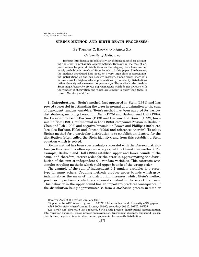
Proof. These can be easily proved by conditioning on the time of the firstjump after leaving the starting state, and producing a recurrence relationusing the fact that the time of transition between states which are two apartis the sum of the times of transition between two adjoining states. It is notnecessary to solve the recurrence relation, just to multiply by πj and add.This is the proof that is given in Keilson [(1979), page 61] for the first formulain (2.11). Alternatively, there is a direct probabilistic proof that reveals theprobability behind these pleasingly simple formulae.

We consider only the case of downward transitions because the other case isentirely similar. Consider a stationary process Z∗ on j j+1 � � � � which hasthe same birth and death parameters as the process on Z+. The distribution ofZ∗�t� for each t is that of π conditioned to be on j j+ 1 � � ��. Define a pointprocess N using Z∗ by inserting a point at an independent exponential(βj)time after each transition into state j, provided the process is still in state jafter the exponential time. Continue the same probabilistic mechanism untilthe process leaves j and record no further points until the process next entersj. The inter-point times are therefore independent and identically distributed,apart from the first one, as after the first one, each inter-point time is theexponential�βj� with probability βj

αj+βjand otherwise is exponential�αj + βj�

plus a geometric number of independent upwards excursion times from j backto j followed by an exponential�βj�. The point process N is stationary, becauseZ∗ is stationary. Let the mean number of points be κ per unit time. Since thecompensator of N is ∫ t

0 βj1�Z∗�s�=j�ds�t≥0,

κ = E�N�1�� =∫ 1

0βjP�Z∗�s� = j�ds = βjπj

F�j� �(2.12)

But κ is then the reciprocal of the mean time between points in the station-ary renewal process N and this is the right hand side of (2.11). The proof iscomplete if we can construct a stationary version of Z in which the times oftransition from j to j− 1 are the inter-point times of N.

Independent of the process Z∗, realize a coin toss with probability of headsF�j�. If the coin is tails, then define Z to coincide with Z∗ up to the first pointof N. If the coin is heads, construct an independent fragment of the uncon-ditional chain which starts in a state distributed according to the conditionaldistribution of π on 0 1 2 � � � j − 1� and finishes at the first entrance toj. Omit, if necessary, the first part of Z∗ up till the time that Z∗ enters jand use the fragment of Z∗ up to the first point of N. The process Z thenhas been defined to start with the stationary distribution π, and it evolvesaccording to the right laws up to the first point of N. Let Z1 Z2 � � � be inde-pendent realisations of fragments of the Markov chain each one consisting ofan excursion of the chain starting in j − 1 and finishing in j. Insert one ofthese fragments after each point of N. The process Z is stationary, Markovand the times between points in Z∗ are precisely the times of transition fromj to j − 1, with the possible exception of the first time. However the strong


0 1 2 3 4 5 6 7 8

2

3

4

5

time

valu

e of

pro

cess

process in state 2if conditionedof occurence =process with ratestationary pointCrosses are

β2

Fig. 1. Birth-death process conditioned to be on 2 3 � � ��

law still shows that the expected time between points is the limiting sampleaverage of the times between points in N, as required.

The process of construction is illustrated in Figures 1–3. ✷

Combining Lemma 2.2 with (2.9) and (2.10) gives the following lemma.

Lemma 2.3. For i ≤ j

gj�i� =−πjF�i− 1�

βiπi

�

0 1 2 3 4 5 6

0

1

2

3

4

time

valu

e of

pro

cess

processpointstationaryof theeach pointadded atinsertionswith{2,3,...}to be onconditionedprocessfromConstructed

Insertion 1 Insertion 2

Fig. 2. Stationary process on whole state space


6543210

4

3

2

1

0

time

valu

e of

pro

cess

conditioned processtimes between the points in theLength of lines with arrows are

to 1transition from 2times oflengths areprocess, theIn the stationary

Fig. 3. Stationary process on whole state space

and for i ≥ j+ 1

gj�i� =πjF�i�αi−1πi−1

�

Lemma 2.4. Let !gj�i� = gj�i+1�−gj�i� and let δi = �βi+1−βi�−�αi+1−αi�� The following are equivalent:

(C0) For each j ∈ Z+, !gj�j� is the only non-negative difference for !gj.

(C1) τ+j is increasing in j and τ−j is decreasing in j. Here and in the se-quel, we use increasing to mean non-decreasing and decreasing to mean non-increasing.

(C2) For each k = 1 2 � � �,

F�k�F�k− 1� ≥

αk

βk

≥ F�k+ 1�F�k� �(2.13)

(C3) For each k = 1 2 � � �,

δk−1 ≥−∑k−2

l=0 δlF�l�F�k− 1�(2.14)

and

δk ≥−∑∞

l=k+1 δlF�l+ 1�F�k+ 1� �(2.15)

In particular, a sufficient condition for any of (C0), (C1), (C2) or (C3) is(C4) For each k = 1 2 � � �, defining β0 = 0,

αk − αk−1 ≤ βk − βk−1�

We defer the proof of Lemma 2.4 to the end of this section.


Remark 2.5. If (2.14) holds for all the values up to k − 1, then the righthand side is negative and the condition specifies that δk must be at least acertain negative number determined by δ0, � � � , δk−1 and π0, � � � , πk. Similarlyfor (2.15).

Remark 2.6. Given any probability distribution there is a range of possiblevalues of the birth and death parameters for these conditions to hold. It is easyto construct artificial examples where the conditions do not hold. For example,take π0 = 1

8 , π1 = 12 , α0 = 1, α1 = 10. Then detailed balance in equation (2.1)

gives β1 = 14 and equation (2.14) is not satisfied for k = 1.

Remark 2.7. For the Poisson distribution, as in Barbour, Holst and Jan-son (1992), (C0) is satisfied if the birth rates are constant at the parameter ofthe distribution. This follows immediately from (C4).

Example 2.8. If the birth parameters are decreasing and the death param-eters are increasing, then (C4) is clearly satisfied and (C0) holds. This exampleis given as Lemma 9.2.1 in Barbour, Holst and Janson (1992). This includesthe Binomial�n p� distribution with αj = �n − j�p, βj = j�1 − p� as notedin Barbour, Holst and Janson (1992). This also includes the Hypergeometricdistribution with parameters R B n ∈ Z+ (n ≤ R+B):

πi =(Ri

)(B

n− i

)/(R+B

n

) max�0 n−B� ≤ i ≤ min�n R�

by taking αj = �n− j��R− j�, βj = j�B− n+ j�.

Example 2.9. For the negative binomial distribution with parameters r >0 and 0 < q < 1:

πi =)�r+ i�)�r�i!

qr�1− q�i i ∈ Z+

and taking αj = a+bj and βj = j with a = r�1−q� and b = 1−q, hence (C4)is satisfied [Brown and Phillips (1999)].

The following proposition provides non-uniform bounds for the solution gto Stein equation (2.3).

Theorem 2.10. Any of (C0)–(C4) implies that the solution g to Stein equa-tion (2.3) satisfies

supf∈�

!g�i� = F�i+ 1�αi

+ F�i− 1�βi

(2.16)

≤ 1αi

∧ 1βi

∀i ∈ Z+�(2.17)


Proof. Replacing f by 1−f if necessary, it suffices to give an upper boundfor !g�i�� Using (2.19) gives

!g�i� =∞∑j=0

f�j�!gj�i��(2.18)

Lemma 2.4 ensures that the only positive term in the right hand side of (2.18)is for j = i, leading to

!g�i� ≤ !gi�i��

Now, (2.16) follows immediately from Lemma 2.3.Finally, since (C2) implies that F�i − 1�/βi ≤ F�i�/αi and F�i + 1�/αi ≤

F�i�/βi, the claim (2.17) is evident. ✷

Remark 2.11. One may ask, as happened in the Poisson approximationcase, whether the bound (2.16) is decreasing in i so that a uniform bound couldbe achieved at i = 0 from conditions (C0)–(C4). Unfortunately, the answeris generally negative. For example, if we take π as Binomial�n p� so thatαi = �n− i�p and βi = �1−p�i for 0 ≤ i ≤ n, then supf∈� !g�0� = �1− �1−p�n�/�np� and supf∈� !g�n� = �1 − pn�/�n�1 − p��, hence supf∈� !g�i� isnot decreasing if p > 1/2.

However, in the special case where the α’s are a constant and the β’s are in-creasing, the case i = 0 is the maximum. This includes Poisson approximation[see Barbour and Eagleson (1983)] and certain other polynomial birth-deathdistributions as shown in section 3.

Corollary 2.12. If αj = α for all j ∈ Z+ and βj is increasing, then

supf∈�

!g�i� ≤ 1− π0

α∀ i ∈ Z+�

Proof [cf. Xia (1999)]. In fact,

supf∈�

!g�i� = 1− π0

α+ π0 + � � �+ πi−1

βi

− π1 + � � �+ πi

α

= 1− π0

α+

i∑j=1

πj

α

(βj

βi

− 1)

≤ 1− π0

α

completing the proof. ✷

To end this section, we give a proof for Lemma 2.4.


Proof of Lemma 2.4. Noting that the solution g to (2.3) satisfies

g�k� =∞∑i=0

f�i�gi�k� (2.19)

and if f is 1, the solution is g = 0, we have

!gj�j� +∑i�=j

!gi�j� = 0�

Condition (C0) is equivalent to all differences except !gj�j� being negative.For i ≤ j− 1, from Lemma 2.1 and (2.11) we have

!gj�i� = −πj

(τ+i − τ+i−1

)�(2.20)

Similarly, for i ≥ j+ 1

!gj�i� = πj

(τ−i+1 − τ−i

)�(2.21)

Considering equations (2.20) and (2.21) and allowing j to vary shows that(C0) is equivalent to (C1).

On the other hand, it follows from (2.11) that, for k = 1 2 3 � � � τ+k−1 ≤ τ+kand τ−k ≥ τ−k+1 are equivalent to

βkF�k� − αkF�k− 1� ≥ 0(2.22)

and

βkF�k+ 1� − αkF�k� ≤ 0 (2.23)

using the detailed balance relations (2.1). Rearrangement gives the equiva-lence of (C1) and (C2).


But the left side of inequality (2.22) is, using the detailed balance conditionβkπk = αk−1πk−1,

βkF�k� − αkF�k− 1� = βkπk +k−1∑l=0

�βk − αk�πl

= ��βk − βk−1� − �αk − αk−1��πk−1

+βk−1πk−1 +k−2∑l=0


= δk−1πk−1 + ��βk − βk−2� − �αk − αk−2��πk−2

+βk−2πk−2 +k−3∑l=0


= δk−1πk−1 + �δk−1 + δk−2�πk−2

+βk−2πk−2 +k−3∑l=0


= · · ·

=k−1∑l=0

�δk−1 + · · · + δl�πl =k−1∑l=0

δlF�l�

(2.24)

showing that (2.22) is the same as (2.14). We have used the definition of β0 as0 in the second last step of these equalities and collected all the terms withthe same δ in the last. Likewise,

βkF�k+ 1� − αkF�k� = −αkπk +∞∑

l=k+1


= −δkπk+1 − αk+1πk+1 +∞∑

l=k+2


= · · ·(2.25)

= −∞∑

l=k+1

�δk + � � �+ δl−1�πl

= −∞∑

l=k+1

δl−1F�l�

showing that (2.23) is the same as (2.15). This gives the equivalence of (C2)and (C3).

The sufficiency of (C4) follows from the equivalences proved and the factthat (C4) is the same as all the δ’s being non-negative. ✷

3. Approximation to the sum of independent Bernoulli trials. LetXi 1 ≤ i ≤ n be independent indicator random variables with distribution

P�Xi = 1� = 1−P�Xi = 0� = pi 1 ≤ i ≤ n�


Set W = ∑ni=1 Xi, λl =

∑ni=1 p

li, and θl = λl/λ1, l = 1 2 � � � We write λ = λ1.

Define

σk =√√√√ n∑

i=k+1

ρi (3.1)

where ρi is the ith largest number of p1�1− p1�, p2�1− p2�, · · ·, pn�1− pn�.We use � W to denote the distribution of W.

It is well-known that the Poisson distribution provides a good approxima-tion to � W if all the pi’s are small [see Barbour, Holst and Janson (1992)and references therein]. Barbour and Hall (1984) show, using the Stein-Chenmethod, that

132

min{

1λ 1} n∑

i=1

p2i ≤ dTV�� W Po�λ�� ≤ 1− e−λ

λ

n∑i=1

p2i (3.2)

where Po�ν� stands for the Poisson distribution with mean ν. The order ofPoisson approximation error in the upper and lower bounds is the same.

On the other hand, it is known that compound Poisson signed measures canimprove the approximation precision [see Barbour and Xia (1999) and refer-ences therein]. It is not attractive to approximate any non-negative quantityby a negative one, and signed measures lack standard interpretations of mo-ments. Thus, it is desirable to find an easily calculable probability measurewhich decreases the order of approximation error. Section 2 provides an algo-rithm for finding such approximating probability measures.

Recall that, in estimating Poisson approximation to � W, we take αj = λand βj = j, for j ∈ Z+. Intuitively, if we aim at higher precision than Poissonapproximation, what we need to do is to reduce the variance of the approximat-ing distribution so that the ‘tailored’ stationary distribution fits � W better.One way of doing this is to keep the death rates and reduce the birth ratesto αj = c�m − j�, where c is a constant: this results in binomial approxima-tion [see Ehm (1991) and Barbour, Holst and Janson (1992)]. Another wayis to keep the birth rates as a constant and increase the death rates. Moreprecisely, let

αj = α βj = βj+ j�j− 1�

πj =αj

3ji=1�βi+ i�i− 1��

{1+

∞∑k=1

αk

3ki=1�βi+ i�i− 1��

}−1

j ∈ Z+�

Since both birth and death rates are polynomial functions, we call this dis-tribution a polynomial birth-death distribution with birth rates determinedby α and death rates 0+ β× j+ 1× j�j− 1�, abbreviated as PBD�α�0 β 1�.Accordingly, the Poisson distribution is PBD�α�0 1�, the binomial distributionis PBD�np −p�0 1 − p�, the negative binomial is PBD�r�1 − q� 1 − q�0 1�and hypergeometric is PBD�nR −R− n+ 1 1�0 B− n+ 1 1�. Note that theparameters of the PBD distributions are not uniquely determined.


Theorem 3.1. With the above setup, if

β = λ2λ−12 − 1− 2λ+ 2λ3λ

−12 α = βλ+ λ2 − λ2 (3.3)

then

dTV�� W PBD�α�0 β 1�� ≤ βλ3

ασ1+ 2λλ2

ασ2(3.4)

≤ θ3

σ1+ 2θ2

2

σ2�1− θ2 − θ2/λ� (3.5)

where �3�5� is valid provided θ2 + θ2/λ < 1�

Remark. When λ is large and pi’s are small, σ1 and σ2 are close to√λ,

so the upper bound in (3.5) is asymptotically �θ3 + 2θ22�/√λ� The order of the

bound is as good as that of compound Poisson signed measure approximation[see Barbour and Xia (1999)].

Remark. The parameters were chosen in such a way as to make the boundas small as possible. The error expression is rearranged in such a way that itinvolves only second differences of the solution g to the Stein equation. Theparameter choice is quite crucial and delicate in this: equations (3.6) and (3.7)ensure that various terms have multipliers that match. Interestingly, the ex-act choice given here arose from numerical work as well as algebra. A firstversion had a cruder choice of the β parameter in that the term λ2 was leftout of the right hand side of (3.7). The resulting error expression involved afirst difference as well as a second difference. The resulting calculated exacttotal variation distance between the law of W and the polynomial birth-deathdistribution came to about the same as for binomial. However, computer explo-ration of parameter choice showed that subtracting one from the β parameteryielded a much lower total variation distance. The algebraic reason for thisthen became apparent by re-examining the error expression and giving theresults here.

Remark. Although the particular implementation here uses the indepen-dence of the X’s, a similar expression holds for dependent trials but the randomvariables Wi (resp. Wij) need in general to have the distribution of W −Xi

(resp. W −Xi −Xj) conditional on Xi = 1 (resp. Xi = 1 and Xj = 1). Inpoint process terms, the calculations use the first and second order reducedPalm distributions. It is difficult but not conceptually impossible to extendthe analysis to higher order Palm distributions and to dependent trials. Thiswould involve some degree of case-by-case analysis, with a careful choice ofparameters to match the multipliers in the various terms.

Before we prove the theorem, we present an example to illustrate the per-formance of the PBD approximation.


Example 3.2. Suppose

SX1 ∼ Binomial�70 0�1� SX2 ∼ Binomial�9 1/3�and SX3 ∼ Binomial�2 1/

√2�

are independent random variables and let W = SX1 + SX2 + SX3, thenEW = 11�4142, Var�W�=8.7142. We apply (3.3) to get α = 415�765255 andβ = 25�247555, then the mean and variance of PBD�α�0 β 1� are 11.4142and 8.71390 respectively, and an exact calculation gives

dTV�� W PBD�α�0 β 1�� = 0�00040

[the bound of (3.4) is 0.074692]. However, an exact calculation gives

dTV�� W Po�EW�� = 0�066

(the upper bound of (3.2) is 0.236545) and

dTV�� W Binomial�n p�� = 0�0048

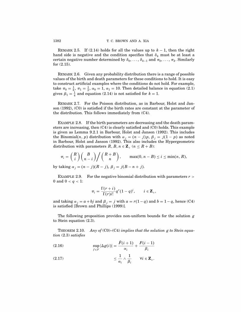
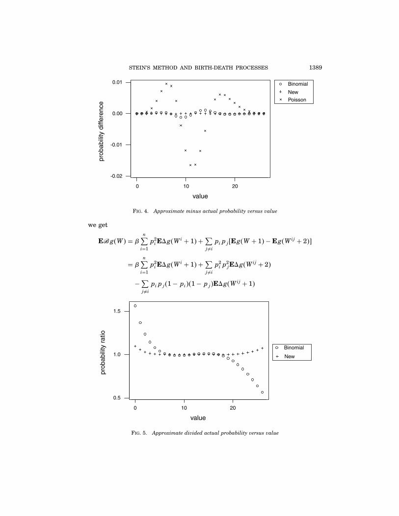
[the upper bound of Theorem 9.E of Barbour, Holst and Janson (1992) is0.218542] with n = 48 and p = 0�237796 so that np = EW and np�1 − p� ≈Var�W�. The PBD(α�0 β 1� approximation is more than 10 times better thanthe binomial approximation, and the binomial approximation does more than10 times better than the Poisson approximation. It is worth noting that thecomputation of PBD distribution is as quick as Poisson and Binomial (in EX-CEL or Minitab, logarithms of PBD probabilities are differences of logarithmsof polynomials; knowledge of means and variances of the actual distributionmakes it easy to pick the range where the probabilities are not essentiallyzero), but it is much harder to calculate the actual probabilities of W (in gen-eral, computation of the probabilities of W is thought to be NP-complete).Figures 4 and 5 provide details of the comparison among the three approxi-mations.

Proof of Theorem 3.1. Set Wi = W −Xi and Wij = W −Xi −Xj, fori j ∈ Z+, i �= j, so that

E�g�W� = αEg�W+ 1� − βEn∑

i=1

pig�Wi + 1� −∑j �=i

pipjEg�Wij + 2�

= βn∑

i=1

p2iE!g�Wi + 1� + �α− βλ�Eg�W+ 1� −∑

j �=ipipjEg�Wij + 2��

Taking

α− βλ = ∑j �=i

pipj = λ2 − λ2 (3.6)


Binomial

New

Poisson

0 10 20

-0.02

-0.01

0.00

0.01

value

prob

abili

ty d

iffer

ence

Fig. 4. Approximate minus actual probability versus value

we get

E�g�W� = βn∑

i=1

p2iE!g�Wi + 1� +∑

j �=ipipj�Eg�W+ 1� −Eg�Wij + 2��

= βn∑

i=1

p2iE!g�Wi + 1� +∑

j �=ip2

ip2jE!g�Wij + 2�

−∑j �=i

pipj�1− pi��1− pj�E!g�Wij + 1�

Binomial

New

0 10 20

0.5

1.0

1.5

value

prob

abili

ty r

atio

Fig. 5. Approximate divided actual probability versus value


= βn∑

i=1

p2iE!g�Wi + 1� +∑

j �=ip2

ip2jE!2g�Wij + 1�

−∑j �=i

pipj�1− pi − pj�E!g�Wij + 1�

where !2g�k� = !g�k+ 1� − !g�k� k ∈ Z+. Let

βλ2 =∑j �=i

pipj�1− pi − pj� = λ2 − λ2 − 2λλ2 + 2λ3�(3.7)

It follows that

E�g�W� = βn∑

i=1

p2iE�!g�Wi + 1� − !g�W+ 1�� +∑

j �=ip2


+∑j �=i

pipj�1− pi − pj�E�!g�W+ 1� − !g�Wij + 1��

= −βn∑

i=1

p3iE!2g�Wi + 1� +∑

j �=ip2


+∑j �=i

pipj�1− pi − pj��pi�1− pj� + pj�1− pi��E!2g�Wij + 1�

+∑j �=i

p2ip

2j�1− pi − pj�E�!2g�Wij + 1� + !2g�Wij + 2��

= −βn∑

i=1

p3iE!2g�Wi + 1�

+∑j �=i

pipj�pi + pj��1− pi��1− pj�E!2g�Wij + 1�

+∑j �=i

p2ip

2j�1− pi − pj�E!2g�Wij + 2��

Noting that

E!2g�Wi + 1� ≤ 2�!g�dTV�� Wi � �Wi + 1�� ≤ �!g�σ1

where �!g� = supk !g�k� [see Barbour and Jensen (1989)], and correspond-ingly

E!2g�Wij + k� ≤ �!g�σ2

∀k ∈ Z+

we obtain

E�g�W� ≤ �!g�{βλ3

σ1+∑

j �=i�pipj�pi + pj��1− pi��1− pj� + p2ip

2j�

σ2

}

≤ �!g�[βλ3

σ1+ 2λλ2

σ2

]


so (3.4) follows from (2.17). Equation (3.5) is due to the facts that α ≥ βλ andα ≥ λ3λ−1

2 − λ− λ2�Finally, (3.3) comes from solving the equations (3.6) and (3.7). ✷

4. Negative binomial approximation to the number of 2-runs. LetJ1 J2 � � � Jn be independent identically distributed Bernoulli random vari-ables with P�Ji = 1� = p, 1 ≤ i ≤ n. To avoid edge effects, we treat i+nj as ifor 1 ≤ i ≤ n j = 0 ±1 ±2 � � � � Define Ii = JiJi−1 and W = ∑n

i=1 Ii. Ourrandom variable of interest is W, which counts the number of 2-runs of Ji,1 ≤ i ≤ n�

The approximation to the number of 2-runs has been well studied pre-viously, see, for example, compound Poisson approximation in total varia-tion in Arratia, Goldstein and Gordon (1990), Roos (1993), Eichelsbacher andRoos (1999) and Barbour and Xia (1999). In this section, we will estimate theaccuracy of negative binomial approximation to � W.

It is easy to establish EIi = p2, EW = np2 and Var�W� = np2�1+2p−3p2�.If p < 2/3, then Var�W� > EW, indicating that, in comparison with Poissonapproximation, we need to either reduce the death rate or increase the birthrate. For simplicity, we increase the birth rate by taking αj = a + bj with0 ≤ b < 1 and βj = j in (2.1). The equilibrium distribution is then a negativebinomial distribution [see Example 2.9]. To keep our notation consistent, wedenote the equilibrium distribution as PBD�a b�0 1�.

Our argument is similar to that in Barbour and Xia (1999). The followingresult can be found as Lemma 5.1 of Barbour and Xia (1999).

Lemma 4.1. Let �ηm m ≥ 1� be independent indicator random variableswith P�ηm = 1� = γm m ≥ 1, and set η0 = 0, that is, γ0 = 0 and Ym =∑m

i=1 ηiηi−1. Then, for each n ≥ 2,

bn�γ1 γ2 � � � γn� = 2dTV�� Yn� � �Yn + 1��≤ 4�6√∑n

i=2�1− γi−2�2γi−1�1− γi−1�γi

�

Now, we state the main result of this section.

Theorem 4.2. Let b = 2p−3p2

1+2p−3p2 and a = �1− b�np2, if p < 2/3, then

dTV�� W� PBD�a b�0 1�� ≤ 32�2p2√�n− 1�p2�1− p�3�

Proof. Let W1 =W− I1− I2− I3. Using the fact that W1, J1 and J2 areindependent, we have

Eg�W+ 1�= Eg�W+ 1��J1J2 + �1−J2�J1 + �1−J1�J2 + �1−J1��1−J2��


= Eg�W1 +Jn +J3 + 2�J1J2� +Eg�W1 +Jn + 1��1−J2�J1�+Eg�W1 +J3 + 1��1−J1�J2� +Eg�W1 + 1��1−J1��1−J2��= E�g�W1 +Jn +J3 + 2� − g�W1 +Jn + 2� − g�W1 +J3 + 2�+g�W1 + 2��J1J2�+E�g�W1 +Jn + 2� − g�W1 +Jn + 1� − g�W1 + 2� + g�W1 + 1��J1J2�+E�g�W1 +J3 + 2� − g�W1 +J3 + 1� − g�W1 + 2� + g�W1 + 1��J1J2�+E�g�W1 +Jn + 1� − g�W1 + 1��J1�+E�g�W1 +J3 + 1� − g�W1 + 1��J2�+E!g�W1 + 1�J1J2� +Eg�W1 + 1�= p2E!2g�W1 + 2�J3Jn� + p2E!2g�W1 + 1��J3 +Jn��+pE!g�W1 + 1��J3 +Jn + p�� +Eg�W1 + 1�

and

EI2g�W�=p2Eg�W1+Jn+J3+1��JnJ3+Jn�1−J3�+J3�1−Jn�+�1−Jn��1−J3��=p2Eg�W1+3�JnJ3+g�W1+2��Jn�1−J3�+�1−Jn�J3�+g�W1+1��1−Jn��1−J3��=p2{E!2g�W1+1�JnJ3�+E!g�W1+1��Jn+J3��+Eg�W1+1�}�

Similarly,

EI2g�W+ 1� = p2E!2g�W1 + 2�JnJ3� + p2E!2g�W1 + 1��Jn +J3��+p2E!g�W1 + 1��Jn +J3 + 1�� + p2Eg�W1 + 1��

Combining the three expansions, we find that

E��a+ bW�g�W+ 1� −Wg�W��= p2�a+ nb�E!2g�W1 + 2�J3Jn�+ p2E!2g�W1 + 1��−nJnJ3 + �a+ nb�Jn + �a+ nb�J3��(4.1)

+E!g�W1 + 1��apJ3 + apJn + ap2 + nbp2�Jn +J3 + 1�− np2�Jn +J3�� + �a− np2 + nbp2�Eg�W1 + 1��

We choose

a = np2�1− b�(4.2)

so that the last term of (4.1) vanishes. Lemma 4.1 may now be applied tobound (4.1). The first term of (4.1) is bounded by

p2�a+ nb�E!2g�W1 + 2�J3Jn�≤ p4�a+ nb�E!2g�W2 +Jn−1 +J4 + 2��≤ p4�a+ nb��!g�bn−2�1 p � � � p 1�


where W2 = W1 − In − I4. By symmetry, the second term of (4.1) can bebounded by

np4E!2g�W2 +Jn−1 +J4 + 1�� + 2�a+ nb�p3E!2g�W3 +Jn−1 + 1��≤ np4�!g�bn−2�1 p � � � p 1� + 2�a+ nb�p3�!g�bn−2�p � � � p 1�

where W3 =W1 − In� Finally, by taking

2�a+ nbp− np� + �a+ nb� = 0 (4.3)

the third term of (4.1) can be reduced to

E!g�W1+1��p�a+nbp−np��J3+Jn�+�a+nb�p2��=p22�a+np�b−1��E!g�W3+Jn−1+1�+�a+nb�E!g�W3+Jn−1Jn+1�=�a+nb�p2E!2g�W3+1�Jn−1�1−Jn��≤�a+nb��1−p�p3E!2g�W4+Jn−2+1��≤�a+nb��1−p�p3�!g�bn−3�p �� p 1�

where W4 =W3 − In−1.Now, we have from Lemma 4.1 that bn−2�1 p � � � p 1�, bn−2�p � � � p 1�

and bn−3�p � � � p 1� are all bounded by

4�6√p2�1− p� + p�1− p�3 + �n− 6�p2�1− p�3

≤ 4�6√�n− 1�p2�1− p�3

since

p2�1− p� + p�1− p�3 ≥ 5p2�1− p�3 0 ≤ p ≤ 1�

The values of a and b follow from (4.2) and (4.3). It is easy to show that con-dition (C4) in Lemma 2.4 is satisfied so Theorem 2.10 gives �!g� ≤ a−1. Theproof is now complete by collecting the three estimates above and simplifyingthe bound. ✷

Remark 4.3. Another way to tackle this problem is to declump the se-quence of J1, � � � , Jn into strings of 1’s separated by 0’s, as discussed in Ar-ratia, Goldstein and Gordon (1990). As each string follows approximately ageometric distribution and the number of strings is roughly binomial, we canapproximate the number of strings of at least two 1’s by an appropriate Pois-son distribution, giving us a bound of order p2. This shows how impressivethe bound in Theorem 4.2 is since it is of order p2/

√np2.

The bound in Theorem 4.2 is as good as that of compound Poisson approx-imation obtained in Barbour and Xia (1999). As a matter of fact, a negativebinomial can also be viewed as a Poisson sum of variables each with logarith-mic distribution [see Johnson, Kotz and Kemp (1992), page 204 ], so the resulthere is also approximation by a compound Poisson distribution. It is surprisingthat the order of approximation seems to be better for this compound Poissonthan the one in Arratia, Goldstein and Gordon (1990).


In general, let Xi ∼Poisson�λi�, i ≥ 1 be independent and set X = X1 +2X2 + 3X3 + · · ·, then X has compound Poisson distribution, denoted asCP�λ1 λ2 � � ��. Our PBD distribution approximation theory developed in sec-tion 2 includes a family of compound Poisson approximations provided λi+1/λi,i ≥ 1 are all small. For example, the following proposition gives an estimatefor the difference between the compound Poisson distribution with two freeparameters and the negative binomial distribution [cf Corollary 4.8 of Barbourand Xia (1999)].

Proposition 4.4. Let λ3 = λ4 = · · · = 0 and define

b = 2λ2

λ1 + 4λ2 a = �λ1 + 2λ2�2

λ1 + 4λ2

then

dTV�CP�λ1 λ2 0 � � �� PBD�a b�0 1�� ≤ 8λ22

�λ1 + 2λ2�2√

2eλ1

�

Proof. In fact,

E�ag�X+ 1� + bXg�X+ 1� −Xg�X��= E�2bλ2g�X+ 3� + �bλ1 − 2λ2�g�X+ 2� + �a− λ1�g�X+ 1��= 2bλ2E�!2g�X+ 1�� + �bλ1 − 2λ2 + 4bλ2�E�g�X+ 2��+�a− λ1 − 2bλ2�E�g�X+ 1��

Take bλ1 − 2λ2 + 4bλ2 = 0 and a − λ1 − 2bλ2 = 0 which are equivalent tob = 2λ2

λ1+4λ2and a = �λ1+2λ2�2

λ1+4λ2 so that the last two terms vanish. Thus,

E�ag�X+ 1� + bXg�X+ 1� −Xg�X��

≤ 4bλ2�!g�dTV�� X� � �X+ 1�� ≤ 8λ22

�λ1 + 2λ2�2√

2eλ1

[see Barbour, Holst and Janson (1992), page 262], completing the proof. ✷

An immediate consequence of the Proposition is that the negative binomialdistribution can approximate the number of 2-runs of W = ∑n

i=1 Ji−1Ji withthe same precision as compound Poisson approximation, even in the case thatJ1 � � � Jn are independent, but not identically distributed, indicators, as in-vestigated in Barbour and Xia (1999). We omit the details of the analysis dueto the complexity of the exercise.

5. Poisson process approximation. The idea presented in section 2can also be extended to solve a counterpart problem in Poisson process ap-proximation. To start with, we recall briefly the notation from Barbour and


Brown (1992) [see also Brown and Xia (1995a)]. Let ) be a compact metricspace with metric d0 bounded by 1, and let � be the space of finite configura-tions on ), that is, the space of integer-valued finite measures on ). For eachξ ∈ � , we use ξ to denote the total number of points of ξ. The metric d1 on� is 1 if the two configurations do not have the same number of points andis otherwise the average d0-distance between the points of the configurationsunder the closest matching. The metric d2 between two probability distribu-tions on � is the infimum of expected values of the d1 distance between anytwo realisations of the probability distributions. Define, for suitable functionh on � , the generator �pp by

�pph�ξ� =∫)�h�ξ + δx� − h�ξ��dx� +

∫)�h�ξ − δx� − h�ξ��ξ�dx��(5.1)

Then �pp is the generator of an � -valued immigration-death process Zξ�t�with immigration intensity � and unit per capita death rate, where Zξ�0� = ξand pp stands for Poisson process. Note that, when ξ = 0, the immigration-death process Zξ is written as Z0� The equilibrium distribution of Zξ is aPoisson process with mean measure �, denoted by Po��. Thus, as in Sec-tion 2, the generator �pp can be used to establish a Stein equation for Po��approximation:

�pph�ξ� = f�ξ� − Po��f� (5.2)

for bounded function f on � . The solution to (5.2) is given by

h�ξ� = −∫ ∞

0�Ef�Zξ�t�� − Po��f��dt(5.3)

[see Barbour and Brown (1992), Proposition 2.3].Let � be the space of all d1-Lipschitz functions f on � , namely, f�ξ1� −

f�ξ2� ≤ d1�ξ1 ξ2� for all ξ1 ξ2 ∈ � (so in particular, since d1 is bounded by1, f is bounded). Then for any point process � on ),

d2�� Po�� = supf∈�

Ef�� − Po��f��

Hence, to use the Stein equation (5.2) in bounding the errors of Po�� approx-imation to � �, we need to estimate

!2h�ξ�x y� = h�ξ + δx + δy� − h�ξ + δx� − h�ξ + δy� + h�ξ� where h is the solution (5.3) to Stein’s equation (5.2), f ∈ � , x y ∈ ). Theo-rem 2.1 of Brown, Weinberg and Xia (2000) gives

!2h�ξ�x y� ≤ 3λ+ 1

n+ 3+ n

λ2+ 1�65

λ1�5n+ 1− λ (5.4)

where n = ξ and λ = ��)��The estimate (5.4) is indeed of optimal order, as demonstrated in a number

of applications in the paper. However, there are four terms in the bound andextra effort is needed in applying the bound in concrete problems. Here, weprove a simplified version of the bound using the techniques from Section 2.


Theorem 5.1. For each f ∈ � , x y ∈ ) and ξ ∈ � with ξ = n, thesolution h of �5�3� satisfies

!2h�ξ�x y� ≤ 5λ+ 3

n+ 1�(5.5)

To prove Theorem 5.1, we need a few technical lemmas. Note that Zξ is abirth-death process with birth rates αi = λ and death rates βi = i, for i ∈ Z+,the notation in section 2 is hence in force, with πi = Po�λ�i��

Lemma 5.2. Let e+n = E exp�−τ+n � and e−n = E exp�−τ−n �, then

e+n =λF�n�

�n+ 1�F�n+ 1� e−n = 1+ n

λ− F�n− 1�

F�n� �(5.6)

Proof. By conditioning on the time of the first jump after leaving theinitial state, we can produce recurrence relations for e+n and e−n :

e+n =λ

λ+ n+ 1− ne+n−1

n ≥ 1� e+0 =λ

λ+ 1�(5.7)

e−n =n+ λ

λ− n− 1

λe−n−1 n ≥ 2� e−1 =

λ+ 1λ

− 1λ∫∞

0 p00�t�e−tdt (5.8)

where p00�t� = P�Z0�t� = 0� [see Wang and Yang (1992), pages 154–156 andpages 174–176]. Now, the claim for e+n follows from (5.7) and mathematicalinduction. On the other hand, it is well-known that Z0�t� ∼ Po �λ�1− e−t��,so

e−1 =λ+ 1λ

− 11− e−λ

�

Using mathematical induction in (5.8) gives the claim for e−n . ✷

Lemma 5.3. If ξ1 = ξ2 = n, then for each f ∈ � , the solution h of �5�3�satisfies

h�ξ1� − h�ξ2� ≤ nd1�ξ1 ξ2�(

1λ+ 1

n+ 1

)�

Proof. Write ξ1 =∑n

i=1 δxiand ξ2 =

∑ni=1 δyi

. Without loss of generality,

we may assume d1�ξ1 ξ2� =∑n

i=1 d0�xi yi�n

� Set ηk =∑k

i=1 δxi+∑n

i=k+1 δyi, 0 ≤

k ≤ n, then η0 = ξ2 and ηn = ξ1. By the triangle inequality, it suffices to showthat

h�ηk� − h�ηk+1� ≤ d0�xk+1 yk+1�(

1λ+ 1

n+ 1

) 0 ≤ k ≤ n− 1�(5.9)


Fix 0 ≤ k ≤ n − 1, and let ψk =∑k

i=1 δxi+ ∑n

i=k+2 δyi. Let S ∼ exp�1� be

independent of Zψkand construct Zηk

�t� = Zψk�t� + δyk+1

1S>t and Zηk+1�t� =

Zψk�t� + δxk+1

1S>t, so that

h�ηk� − h�ηk+1� =∣∣∣∣∫ ∞

0E�f�Zηk

�t�� − f�Zηk+1�t��dt

∣∣∣∣=∣∣∣∣∫ ∞

0e−tE�f�Zψk

�t� + δyk+1� − f�Zψk

�t� + δxk+1��dt

∣∣∣∣≤ d0�xk+1 yk+1�

∫ ∞0

e−tE1

Zψk�t� + 1

dt

≤ d0�xk+1 yk+1�(

1λ+ 1

n+ 1

)

where the last inequality is from Lemma 2.2 of Brown, Weinberg andXia (2000). ✷

The following lemma is taken from a statement in the proof of Lemma 3.2of Brown, Weinberg and Xia (2000).

Lemma 5.4. If ξ1 = ξ2 = n, then for each f ∈ � and x ∈ ),

�h�ξ1 + δx� − h�ξ1�� − �h�ξ2 + δx� − h�ξ2�� ≤2n

n+ 1d1�ξ1 ξ2��

Proof of Theorem 5.1. By conditioning on the first jump time of leavingξ + δx, it follows from (5.3) that

h�ξ + δx� =−�f�ξ + δx� − Po��f��

n+ 1+ λ

+ λ

n+ 1+ λEh�ξ + δx + δV� +

n+ 1n+ 1+ λ

Eh�ξ + δx − δUx�

where V ∼ �/λ and Ux is uniformly distributed on z1 � � � zn x� withz1 � � � zn the atoms of ξ. Rearranging the equation gives

Eh�ξ + δx + δV� =f�ξ + δx� − Po��f�

λ

+n+ 1+ λ

λh�ξ + δx� −

n+ 1λ

Eh�ξ + δx − δUx��

This in turn yields

!2h�ξ�x y� = �h�ξ + δx + δy� −Eh�ξ + δx + δV�� + �h�ξ + δx� − h�ξ + δy��

+�h�ξ� −Eh�ξ + δx − δUx�� + f�ξ + δx� − Po��f�

λ(5.10)

+n+ 1− λ

λ�h�ξ + δx� −Eh�ξ + δx − δUx

��


Swap x and y to get

!2h�ξ�x y� = �h�ξ + δx + δy� −Eh�ξ + δy + δV�� + �h�ξ + δy� − h�ξ + δx��+�h�ξ� −Eh�ξ + δy − δUy

�� + f�ξ + δy� − Po��f�λ

(5.11)

+n+ 1− λ

λ�h�ξ + δy� −Eh�ξ + δy − δUy

��

where Uy is uniformly distributed on z1 � � � zn y�.Adding up (5.10) and (5.11) and then dividing by 2, we obtain∣∣!2h�ξ�x y�∣∣ ≤ max

z=x y∣∣h�ξ + δx + δy� −Eh�ξ + δz + δV�

∣∣+max

z=x y∣∣h�ξ� −Eh�ξ + δz − δUz

�∣∣+max

z=x y

∣∣∣∣f�ξ + δz� − Po��f�λ

∣∣∣∣+max

z=x y

∣∣∣∣n+ 1− λ

λ�h�ξ + δz� −Eh�ξ + δz − δUz

��∣∣∣∣ �

(5.12)

First, using the fact that f is Lipschitz, the third term in (5.12) is clearlybounded by 1/λ� Next, we apply Lemma 5.3 to the first two terms of (5.12) toconclude that each is bounded by 1

λ+ 1

n+1 � Finally, for z = x or y,∣∣∣∣n+ 1− λ


��∣∣∣∣ ≤ 2

λ+ 1

n+ 1(5.13)

so that (5.5) follows from collecting the bounds for the terms in (5.12).

To prove (5.13), it is enough to consider the following two cases.

Case I: n+ 1 > λ. Let τ−n+1 = inft Zξ+δz�t� = n�. Then using strong

Markov property gives

h�ξ + δz� = −E∫ τ−n+1

0�f�Zξ+δz

�t�� − Po��f��dt+Eh�ζ�

where ζ = Zξ+δz�τ−n+1�� Consequently,∣∣∣∣n+ 1− λ


��∣∣∣∣

≤ n+ 1− λ

λEτ−n+1 +

n+ 1− λ

λEh�ζ� −Eh�ξ + δz − δUz

��(5.14)

However, by (2.11) and Proposition A.2.3 of Barbour, Holst and Janson (1992),

n+ 1− λ

λEτ−n+1 =

�n+ 1− λ�F�n+ 1�λ�n+ 1�Po�λ�n+ 1� ≤

�n+ 1− λ��n+ 2�λ�n+ 1��n+ 2− λ� ≤

1λ�(5.15)

The second term of (5.14) depends on the difference between ζ and ξ+δz−δUz.

For convenience, write z as zn+1 and realize Zξ+δzfrom

Zξ+δz�t� = Z0�t� +

n+1∑i=1

δzi1Si>t


where S1 � � � Sn+1 are independent exp(1) random variables and independentof Z0. At time τ−n+1,

∑n+1i=1 1Si>τ−n+1

of z1 � � � zn+1 are still alive and at least one ofthem has died. Since the death can happen to z1 � � � zn+1 with equal chance,we can construct a coupling such that

ξ + δz −n+1∑i=1

δzi1Si>τ−n+1

=n+1∑i=1

δzi1Si≤τ−n+1

= δUz+ η

with random element η ∈ � . Under this coupling,

ξ + δz − δUz= η+

n+1∑i=1

δzi1Si>τ−n+1

giving

nd1�ξ + δz − δUz ζ� ≤ Z0�τ−n+1��(5.16)

On the other hand,

EZ0�τ−n+1� = n−En+1∑i=1

1Si>τ−n+1= n− �n+ 1�P�S1 > τ−n+1��

Noting that S1 > τ−n+1 is equivalent to

S1 > inf

{t Z0�t� +

n+1∑i=2

1Si>t = n− 1

} = τ−n

and S1 is independent of τ−n , we have from (5.6) that

EZ0�τ−n+1�=n−�n+1�Eexp�−τ−n �=−1+�n+1�(F�n−1�F�n� − n

λ

)�(5.17)

Now, we claim that

n+ 1− λ

λEZ0�τ−n+1� ≤ 1�(5.18)

In fact, by (5.17), (5.18) is equivalent to

�n+ 1− λ��λF�n− 1� − nF�n�� − λF�n� ≤ 0�

Expanding the formula into a power series of λ, we have that (5.18) is thesame as

∞∑i=n+1

λi

�i− 1�! �2n+ 1− i− �n+ 1�n/i� ≤ 0

which is obviously true.


Thus, it follows from Lemma 5.3, (5.16) and (5.18) that the second term of(5.14) is bounded by

n+ 1− λ

λEh�ζ� −Eh�ξ + δz − δUz

�

≤ n+ 1− λ

λEZ0�τ−n+1�

(1λ+ 1

n+ 1

)≤ 1

λ+ 1

n+ 1�

(5.19)

Combining (5.15) and (5.19) yields (5.13).

Case II: n+ 1 ≤ λ. Likewise, let τ+n = inft Zξ+δz−δUz�t� = n + 1�, then

we get from strong Markov property that

h�ξ + δz − δUz� = −E

∫ τ+n

0�f�Zξ+δz−δUz

�t� − Po��f��dt+Eh�ς�

where ς = Zξ+δz−δUz�τ+n �� Hence∣∣∣∣n+ 1− λ


��∣∣∣∣

≤ λ− �n+ 1�λ

Eτ+n +λ− �n+ 1�

λEh�ς� −Eh�ξ + δz��

(5.20)

Using (2.11) and Proposition A.2.3 of Barbour, Holst and Janson (1992) again,we have

λ− �n+ 1�λ

Eτ+n =�λ− �n+ 1��F�n�

λ2Po�λ�n� ≤ �λ− �n+ 1��λλ2�λ− n� ≤ 1

λ�(5.21)

To estimate the second term of (5.20), without loss of generality, we may as-sume Uz = zn+1 and realize

Zξ�t� = Z0�t� +n∑

i=1

δzi1Si>t

where S1 � � � Sn and Z0 are as in Case I. At time τ+n , there are∑n

i=1 1Si>τ+n ofz1 � � � zn still alive, so

�n+ 1�d1�ξ + δz ς� ≤ Z0�τ+n ��(5.22)

But

EZ0�τ+n � = n+ 1−En∑

i=1

1Si>τ+n = n+ 1− nP�S1 > τ+n ��

Since S1 > τ+n is equivalent to

S1 > inf

{t Z0�t� +

n∑i=2

1Si>t = n

} = τ+n−1

and S1 is independent of τ+n−1, we get from (5.6) that

EZ0�τ+n � = n+ 1− nE exp�−τ+n−1� = 1+ nF�n� − λF�n− 1�F�n� �(5.23)


We now show

λ− �n+ 1�λ

EZ0�τ+n � ≤ 1�(5.24)

Using (5.23), (5.24) can be rewritten as

�λ− �n+ 1��nF�n� − λF�n− 1�� ≤ �n+ 1�F�n� which can be verified by rearranging the terms into a series of λ, as in Case I.

Applying Lemma 5.3, (5.22) and (5.24), it follows that

λ− �n+ 1�λ

Eh�ς� −Eh�ξ + δz�

≤ λ− �n+ 1�λ

EZ0�τ+n �(

1λ+ 1

n+ 1

)≤ 1

λ+ 1

n+ 1

which, together with (5.20) and (5.21), gives (5.13). ✷

The implication of the improved estimate (5.5) is that the calculations forbounding the errors of Poisson process approximation in terms of d2-metriccan be significantly simplified. To illustrate the degree of simplification, wepresent a theorem based on Palm processes.

Recall that for a point process � with mean measure � the point process �x

is said to be a Palm process associated with � at x ∈ ) if for any measurablefunction f )×� �→ �0 ∞�,

E(∫

)f�x ��dx�

)= E

(∫)f�x �x��dx�

)

[see Kallenberg (1976)]. The process �x−δx is called the reduced Palm process.The metric we shall use for bounding the approximation errors is d′′1 as

introduced in Brown and Xia (1995a): for ξ1 =∑n

i=1 δxi, ξ2 =

∑mi=1 δyi

∈ �with m ≥ n,

d′′1�ξ1 ξ2� = min�

n∑i=1

d0�xi y� �i�� + �m− n�

where � ranges over all permutations of �1 � � � m�� Note that d′′1�ξ1 ξ2� ≤�ξ1 − ξ2�, the total variation norm of the signed measure ξ1 − ξ2. Also, ifξ1 = ξ2 = n, then d′′1�ξ1 ξ2� = nd1�ξ1 ξ2�� This results in

Lemma 5.5. For ξ η ∈ � and x ∈ ),

�h�ξ + δx� − h�ξ�� − �h�η+ δx� − h�η��

≤ 2η ∧ ξ + 1

�d′′1�ξ η� −∣∣η − ξ∣∣� + (5

λ+ 3η ∧ ξ + 1

) ∣∣η − ξ∣∣≤(

5λ+ 3η ∧ ξ + 1

)d′′1�ξ η��


Proof. Write ξ = ∑ni=1 δxi

and η = ∑mi=1 δyi

. Without loss of generality,we assume m ≥ n and

d′′1�ξ η� =n∑

i=1

d0�xi yi� + �m− n��

Define η′ =∑ni=1 δyi

, then

�h�ξ + δx� − h�ξ�� − �h�η+ δx� − h�η��≤ �h�ξ + δx� − h�ξ�� − �h�η′ + δx� − h�η′��+ �h�η′ + δx� − h�η′�� − �h�η+ δx� − h�η��

The proof is then complete by applying Lemma 5.4 and Theorem 5.1. ✷

As an immediate application of Lemma 5.5, we now state a theorem forestimating the errors of Poisson process approximation in terms of Palm pro-cesses.

Theorem 5.6. Let � be a finite point process on ) with mean measure �.Suppose for each x ∈ ) that �x is the Palm process associated with � at x.Then

d2�� Po�� ≤ E∫)

2�∧�x−δx+1

�d′′1�� x−δx�−∣∣�−�x−δx

∣∣��dx�+E

∫)

(5λ+ 3�∧�x−δx+1

)∣∣�−�x−δx∣∣��dx�(5.25)

≤ E∫)

(5λ+ 3�∧�x−δx+1

)d′′1�� x−δx��dx��(5.26)

Remark 5.7. These simplified bounds, with only one integrand in (5.26),are to be compared with Theorem 3.1 of Brown, Weinberg and Xia (2000),which has three terms to compute. Thus, Theorem 5.6 is more applicable andthe order of the estimated bounds will be the same as that obtained fromTheorem 3.1 of Brown, Weinberg and Xia (2000).

Acknowledgments. Many thanks to Louis H. Y. Chen and Kwok PuiChoi for many useful conversations and splendid hospitality. The work wasdone when Aihua Xia was a member of the Department of Statistics, TheUniversity of New South Wales, Sydney 2052, Australia.

After acceptance subject to revision of this paper, the authors learned thata former Ph.D student of Brown, G Weinberg, had submitted and obtainedacceptance of a paper “Stein factor bounds for random variables” in Journalof Applied Probability. The work that Weinberg reports extends the work inXia (1999) and the results are less general than those here.


REFERENCES

Arratia, R., Goldstein, L. and Gordon, L. (1989). Two moments suffice for Poisson approxima-tions: the Chen-Stein method Ann. Probab. 17 9–25.

Arratia, R., Goldstein, L. and Gordon, L. (1990). Poisson approximation and the Chen-Steinmethod. Statist. Sci. 5 403–434.

Barbour, A. D. (1988). Stein’s method and Poisson process convergence. J. Appl. Probab. 25 175–184.

Barbour, A. D. and Brown, T. C. (1992). Stein’s method and point process approximation. Stochas-tic Processes Appl. 43 9–31.

Barbour, A. D., Chen, L. H. Y. and Loh, W. (1992). Compound Poisson approximation for non-negative random variables using Stein’s method. Ann. Probab. 20 1843–1866.

Barbour, A. D. and Eagleson, G. K. (1983). Poisson approximation for some statistics based onexchangeable trials. Adv. Appl. Prob. 15 585–600.

Barbour, A. D. and Hall, P. (1984). On the rate of Poisson convergence. Math. Proc. CambridgePhilos. Soc. 95 473–480.

Barbour, A. D., Holst, L. and Janson, S. (1992). Poisson Approximation. Oxford Univ. Press.Barbour, A. D. and Jensen, J. L. (1989). Local and tail approximations near the Poisson limit.

Scandinavian J. Statist. 16 75–87.Barbour, A. D. and Xia, A. (1999). Poisson perturbation. ESAIM: Probab. Statist. 3 131–150.Brown, T. C. and Phillips, M. J. (1999). Negative binomial approximation with Stein’s method.

Method. Comput. Appl. Probab. 1 407–421.Brown, T. C., Weinberg, G. V. and Xia, A. (2000). Removing logarithms from Poisson process

error bounds. Stochastic Processes Appl. 87 149–165.Brown, T. C. and Xia, A. (1995a). On metrics in point process approximation. Stochastics Stochas-

tics Rep. 52 247–263.Brown, T. C. and Xia, A. (1995b). On Stein-Chen factors for Poisson approximation. Statist.

Probab. Lett. 23 327–332.Chen, L.H.Y. (1975). Poisson approximation for dependent trials. Ann. Probab. 3 534–545.Ehm, W. (1991). Binomial approximation to the Poisson binomial distribution. Statist. Probab.

Lett. 11 7–16.Eichelsbacher, P. and Roos, M. (1999). Compound Poisson approximation for dissociated random

variables via Stein’s method. Combin. Probab. Comput. 8 335–346.Johnson, N. L., Kotz, S. and Kemp, A. (1992). Univariate Discrete Distributions. Wiley, New York.Kallenberg, O. (1976). Random Measures. Academic Press, New York.Keilson, J. (1979). Markov Chain Models–Rarity and Exponentiality. Springer, New York.Loh, W. (1992). Stein’s method and multinomial approximation. Ann. Appl. Probab. 2 536–554.Roos, M. (1993). Stein–Chen method for compound Poisson approximation. Ph.D. dissertation,

Univ. Zurich.Stein, C. (1971). A bound for the error in the normal approximation to the distribution of a sum

of dependent random variables. Proc. Sixth Berkeley Symp. Math. Statist. Probab. 3583–602. Univ. California Press, Berkeley.

Wang, Z. and Yang, X. (1992). Birth and Death Processes and Markov Chains. Springer, NewYork.

Xia, A. (1999). A probabilistic proof of Stein’s factors. J. Appl. Probab. 36 287–290.

Department of Mathematics and StatisticsUniversity of MelbourneParkville, VIC 3010AustraliaE-mail: [email protected]

bytimothyc.brownandaihuaxia universityofmelbourne

Documents