© v. sanchez & a. basu, university of alberta standard...

© V. Sanchez & A. Basu, University of Alberta

The JPEG2000 Image Compression

Standard


Part I: Image Compression

Compression techniques are used to reduce the redundant information in the image data in order to facilitate the storage, transmission and distribution of images (e.g. GIF, TIFF, PNG, JPEG)


Limitations of JPEG Standard

� Low bit-rate compression: JPEG offers an excellent quality at high and mid bit-rates. However, the quality is unacceptable at low bit-rates (e.g. below 0.25 bpp)

� Lossless and lossy compression: JPEG cannot provide a superior performance at lossless and lossy compression in a single code-stream.

� Transmission in noisy environments: the current JPEG standard provides some resynchronization markers, but the quality still degrades when bit-errors are encountered.

�Different types of still images: JPEG was optimized for natural images. Its performance on computer generated images and bi-level (text) images is poor.


Part II: The JPEG2000 Image Compression Standard


What is JPEG2000?

• JPEG2000 is a new compression standard for still images intended to overcome the shortcomings of the existing JPEG standard.

• The standardization process is coordinated by the Joint Technical Committee on Information technology of the International Organization for Standardization (ISO)/ International Electrotechnical Commission (IEC).

• JPEG2000 makes use of the wavelet and sub-band technologies. Some of the markets targeted by the JPEG2000 standard are Internet, printing, digital photography, remote sensing, mobile, digital libraries and E-commerce.

• The core compression algorithm is primarily based on the Embedded Block Coding with Optimized Truncation (EBCOT) of the bit-stream. The EBCOT algorithm provides a superior compression performance and produces a bit-stream with features such as resolution and SNR scalability and random access.


Features of JPEG2000

� Lossless and lossy compression: the standard provides lossycompression with a superior performance at low bit-rates. It also provides lossless compression with progressive decoding. Applications such as digital libraries/databases and medical imagery can benefit from this feature.

� Protective image security: the open architecture of the JPEG2000 standard makes easy the use of protection techniques of digital images such as watermarking, labeling, stamping or encryption

� Region-of-interest coding: in this mode, regions of interest (ROI’s) can be defined. These ROI’s can be encoded and transmitted with better quality than the rest of the image .

� Robustness to bit errors: the standard incorporate a set of error resilient tools to make the bit-stream more robust to transmission errors.


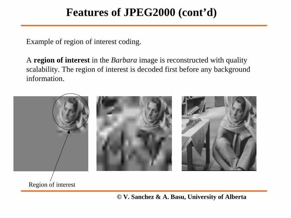
Example of region of interest coding.

A region of interest in the Barbara image is reconstructed with quality scalability. The region of interest is decoded first before any background information.

Features of JPEG2000 (cont’d)

Region of interest


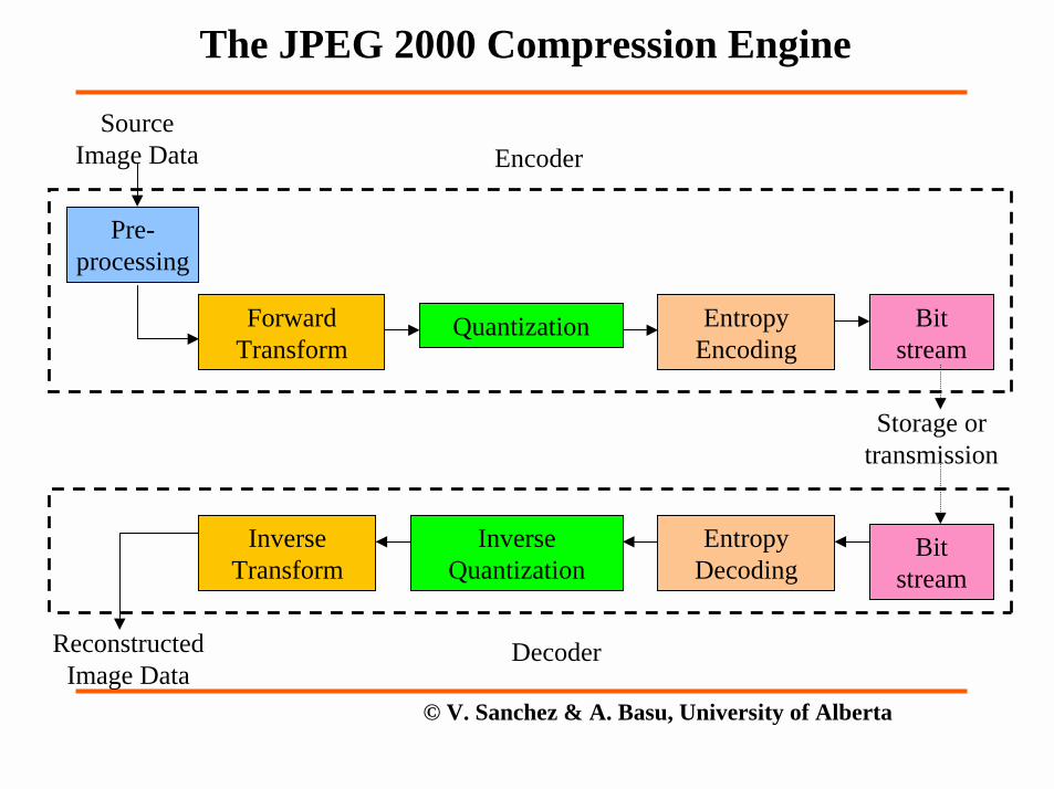
Pre-processing

Forward Transform

Quantization Entropy Encoding

Inverse Transform

Inverse Quantization

Entropy Decoding

Bit stream

Bit stream

Storage or transmission

Reconstructed Image Data

Source Image Data

Decoder

Encoder

The JPEG 2000 Compression Engine


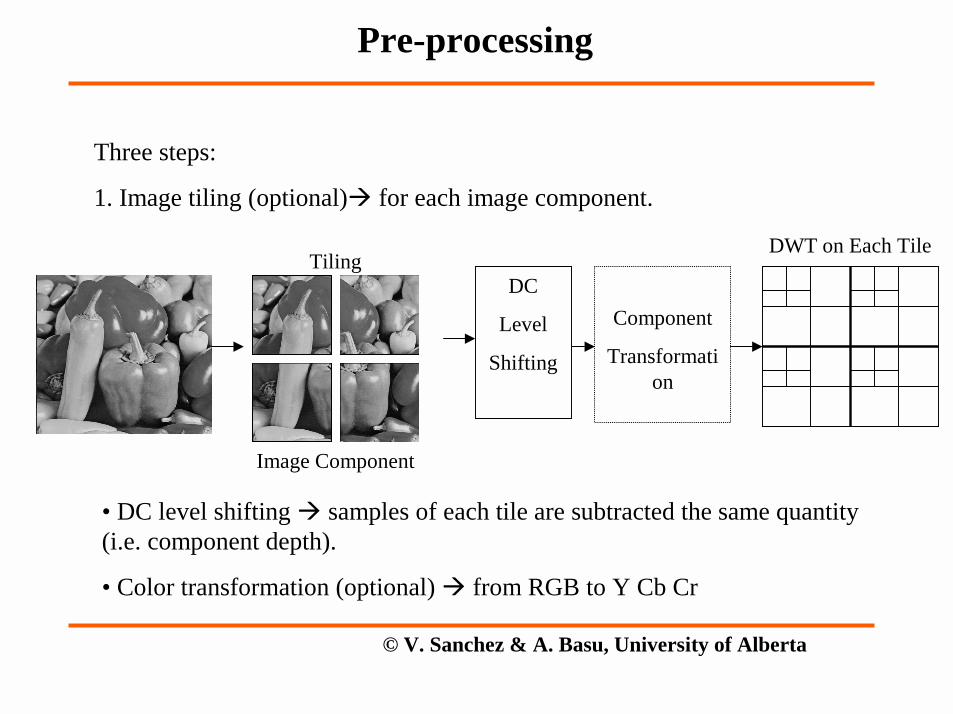
Three steps:

1. Image tiling (optional)� for each image component.

• DC level shifting � samples of each tile are subtracted the same quantity (i.e. component depth).

• Color transformation (optional) � from RGB to Y Cb Cr

DC

Level

Shifting

Component

Transformation

TilingDWT on Each Tile

Image Component

Pre-processing


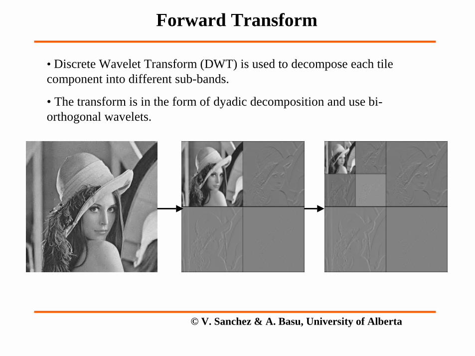
• Discrete Wavelet Transform (DWT) is used to decompose each tile component into different sub-bands.

• The transform is in the form of dyadic decomposition and use bi-orthogonal wavelets.

Forward Transform


• DWT can be irreversible or reversible.

� Irreversible transform �Daubechies 9-tap/7-tap filter

� Reversible transform � Le Gall 5-tap/3-tap filter

• Two filtering modes are supported:

� Convolution based

� Lifting based

Forward Transform (cont’d)


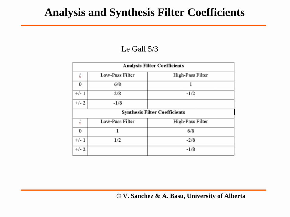
Analysis and Synthesis Filter Coefficients

Le Gall 5/3


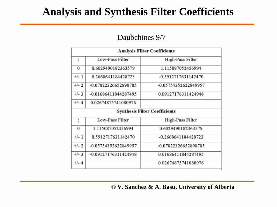
Analysis and Synthesis Filter Coefficients

Daubchines 9/7


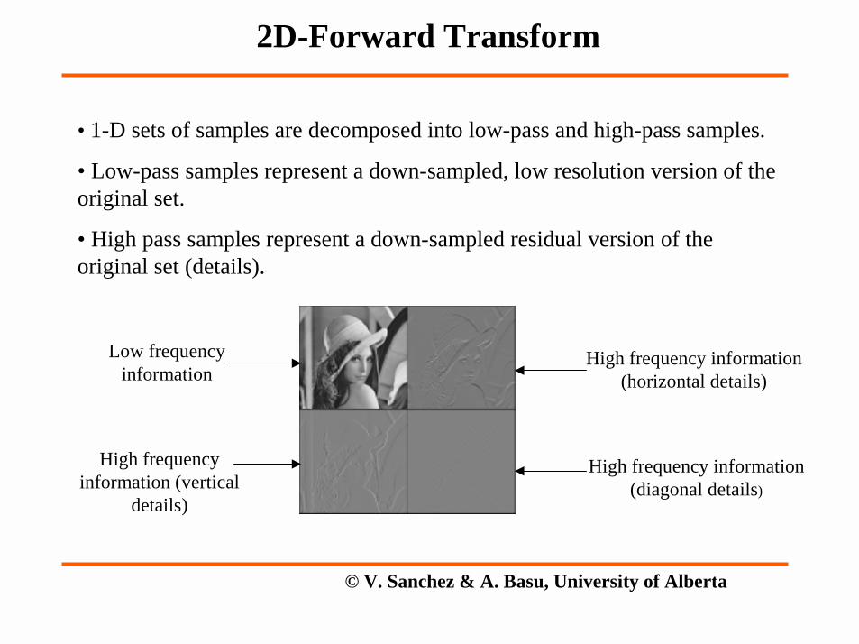
• 1-D sets of samples are decomposed into low-pass and high-pass samples.

• Low-pass samples represent a down-sampled, low resolution version of the original set.

• High pass samples represent a down-sampled residual version of the original set (details).

Low frequency information

High frequency information (horizontal details)

High frequency information (diagonal details)

High frequency information (vertical

details)

2D-Forward Transform


• After transformation, all coefficients are quantized using scalar quatization.

• Quantization reduces coefficients in precision. The operation is lossy unless the quatization step is 1 and the coefficients integers (e.g. reversible integer 5/3 wavelet).

• The process follows the formula:

∆=

b

bbb

vuavuasignvuq

),()),((),(

Quantization stepQuantized value

Largest integer not exceeding ab

Transform coefficient of sub-band b

Quantization


Modes of Quantization

• Two modes of operation:

� Integer mode� integer-to-integer transforms are employed. Quantization step are fixed to one. Lossy coding is still achieved by discarding bit-planes.

� Real mode� real-to-real transforms are employed. Quantization steps are chosen in conjunction with rate control. In this mode, lossy compression is achieved by discarding bi-planes or changing the size of the quantization step or both.


Each code-block forms the input to the entropy encoder and is encoded independently.

Precinct: each sub-band is divided into rectangular blocks called precincts.

Packets: three spatially consistent rectangles comprise a packet.

Code-block: each precinct is further divided into non-overlapping rectangles called code-blocks.

Within a packet, code-blocks are visited in raster order.

1 2

3 4

5 6

7 8

9 10

11 12

Packet PrecinctCode-block

Sub-band

Code-blocks, precincts and packets


15 6

113 1111

101111003010611115LSBMSB

Bit-plane context based arithmetic

coderEncoded data

Bit-plane representation

Coding passes

Code-block

• The coefficients in a code block are separated into bit-planes. The individual bit-planes are coded in 1-3 coding passes.

Entropy Coding: Bit-planes


• Each of these coding passes collects contextual information about the bit-plane data. The contextual information along with the bit-planes are used by the arithmetic encoder to generate the compressed bit-stream.

• The coding passes are:

� Significance propagation pass � coefficients that are insignificant and have a certain preferred neighborhood are coded.

� Magnitude refinement pass � the current bits of significant coefficients are coded.

� Clean-up pass � the remaining insignificant coefficients for which no information has yet been coded are coded.

Entropy Coding: Coding Passes


• For each code-block, a separate bit-stream is generated.

• The coded data of each code-block is included in a packet.

• If more that one layer is used to encode the image information, the code-block bit-streams are distributed across different packets corresponding to different layers.

H

H

Coded code-block

Packet

Layer

JPEG2000 bit-stream

JPEG2000 Bit-stream

Main Header

Packet Header


• Therefore, each layer consists of a number of consecutive bit-plane coding passes from each code-block in the tile, including all sub-bands of all components for that tile.

Layers of the JPEG2000 Bit-stream


Layer Formation

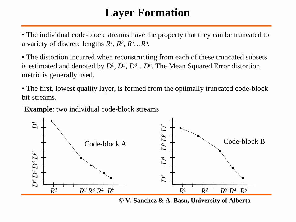
• The individual code-block streams have the property that they can be truncated to a variety of discrete lengths R1, R2, R3…Rn.

• The distortion incurred when reconstructing from each of these truncated subsets is estimated and denoted by D1, D2, D3…Dn. The Mean Squared Error distortion metric is generally used.

• The first, lowest quality layer, is formed from the optimally truncated code-block bit-streams.

R1 R2 R3 R4 R5

D5 D

4 D

3D

2D

1

R1 R2 R3 R4 R5

D5

D4

D

3 D

2D

1

Code-block A Code-block B

Example: two individual code-block streams


• Each subsequent layer is formed by optimally truncating the code-block bit-streams to achieve successively higher target bit-rates, distortion bounds or other quality metrics, as appropriate, and including the additional code words required to augment the information represented in previous layers to the new truncation points.

R1 R2 R3 R4 R5

D5 D

4 D

3D

2D

1

R1 R2 R3 R4 R5D

5

D

4

D3 D

2D

1

Code-block ACode-block B

If target rate for layer 1 is RL1 and 123

LBA RRR ≈+ with a minimum distortion;then, code-block A is truncated to R3 and code-block B is truncated to R2 for layer 1.

Code-block contributions

Example:


Single-quality-layer compression Multiple-quality-layer compression

Main Header

Packet 1

Packet 2

Packet 3

Packet k

Packet k-1

Low frequency sub-band

coefficients

High frequency sub-band

coefficients

.

.

.

.

.

Main Header

Packet 1

Packet 2

Packet 3

Packet k

Packet k-1

Most important bit-planes

Least important bit-planes

.

.

.

.

.

Hierarchical structure of the JPEG2000 Bit-stream


0.125 bpp 0.25 bpp 0.5 bpp

The Barbara image is decompressed at different qualities.

Quality ScalabilityBy interleaving the packets in different orders, four possible progression orders can be achieved in JPEG2000:

• Quality

• Resolution

• Spatial location

• Component


The Barbara image is reconstructed at three resolutions.

Resolution Scalability


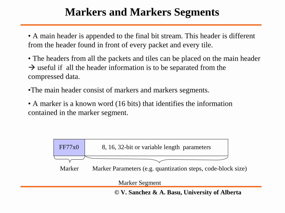
• A main header is appended to the final bit stream. This header is different from the header found in front of every packet and every tile.

• The headers from all the packets and tiles can be placed on the main header � useful if all the header information is to be separated from the compressed data.

•The main header consist of markers and markers segments.

• A marker is a known word (16 bits) that identifies the information contained in the marker segment.

Marker Marker Parameters (e.g. quantization steps, code-block size)

Marker Segment

FF77x0 8, 16, 32-bit or variable length parameters

Markers and Markers Segments


• A header is placed in front of every packet and contains the following information :

� Zero length packet �indicates whether the packet has a length of zero or not.

� Code-block inclusion �indicates whether a code block has been included in the packet or not.

� Zero-bit plane information �if a code-block is included for the first time, the packet header contains information identifying the actual number of bit-planes used to represent coefficients from the code-block.

� Number of coding passes �the number of coding passes included in this packet from each code-block.

� Length of data from a given code block �the packet header identifies the number of bytes contributed by each included code-block.

• The information in the packet header is variable length encoded.

Packet Headers


• For a 512 x 512 gray-level image compressed with one tile, code-block size 64 x 64, precinct size 512 x 512, 3 levels of decomposition and one layer, the general structure of the bit stream is as follows

Main Header Packet 0 Packet 1 Packet 2

Packet Header 0

Packet Header 1

Packet Header 2

Tile Header 0

End of code stream marker

• If all the packet headers are grouped together in a single header and placed in the main header, the structure is:

Main Header Packet 0 Packet 1 Packet 2

Packet Header 0

Packet Header 1

Packet Header 2

Tile Header 0End of code

stream marker

Sample JPEG2000 bit-stream


• The main header would include the following markers and marker segments:

SOC: Start of Code Stream marker

SIZ: Image and Tile Size marker

The SIZ marker segment provides information about the size of the uncompressed image.COD: Coding Style Default marker

The COD marker segment provides information about the coding style, decomposition and layering used for all the components of the imageQCD: Quantization Default marker

The QCD marker segment provides information about the quantization used for all the components of the imagePPM: Packed Packet Headers, main header

The PPM marker segment is the collection of packet headers.

SOD: Start of Data marker

EOC: End of Code Stream marker

SOT: Start of Tile-part marker

The SOT marker segment marks the beginning of a tile-part

Main header

Tile-part header

Compressed date

Markers in a JPEG2000 bit-stream

© v. sanchez & a. basu, university of alberta standard...

Documents