ՀԱՅ - science.rau.amscience.rau.am/uploads/blocks/0/7/701/files/vestnik_2018-2.pdf · variation...
TRANSCRIPT


ՀԱՅ-ՌՈՒՍԱԿԱՆ ՀԱՄԱԼՍԱՐԱՆ
Լ Ր Ա Բ Ե Ր ՀԱՅ-ՌՈՒՍԱԿԱՆ ՀԱՄԱԼՍԱՐԱՆԻ
ՍԵՐԻԱ
ՖԻԶԻԿԱՄԱԹԵՄԱՏԻԿԱԿԱՆ
ԵՎ ԲՆԱԿԱՆ ԳԻՏՈՒԹՅՈՒՆՆԵՐ
№ 2
ՀՌՀ Հրատարակչություն
Երևան 2018

РОССИЙСКО-АРМЯНСКИЙ УНИВЕРСИТЕТ
В Е С Т Н И К РОССИЙСКО-АРМЯНСКОГО
УНИВЕРСИТЕТА
СЕРИЯ:
ФИЗИКО-МАТЕМАТИЧЕСКИЕ И ЕСТЕСТВЕННЫЕ НАУКИ
№ 2
Издательство РАУ
Ереван 2018

Печатается по решению Ученого совета РАУ
Вестник РАУ, № 2. – Ер.: Изд-во РАУ, 2018. – ********** с.
Редакционная коллегия:
Главный редактор Амбарцумян С.А. Зам. главного редактора Аветисян П.С. Ответственный секретарь Шагинян Р.С.
Члены редколлегии:
О.В. Бесов, В.И. Буренков, Г.Р. Вардапетян, М.А. Давтян, Г.Г. Данагулян, И.Д. Заславский, Г.Г. Казарян, Э.М. Казарян, Г.А. Карапетян, Б.И. Коноплев, Г.Б. Маранджян, Р.Л. Мелконян, В.И. Муронец, Б.С. Нагапетян, С.Г. Петросян, А.А. Саркисян, Г.З. Саркисян, А.Г. Сергеев Журнал входит в перечень периодических изданий, зарегистрированных ВАК РА Российско-Армянский университет, 2018 г. ISBN 1829-0450
© Издательство РАУ, 2018

Вестник РАУ № 2, 2018, 5-16 5
МАТЕМАТИКА И ИНФОРМАТИКА
УДК: 519.23
COMPARATIVE STUDY OF THREE APPROACHES
FOR ESTIMATING THE WEIBULL DISTRIBUTION
PARAMETERS
D. Asatryan
Russian-Armenian University Institute for Informatics and Automation Problems of NAS RA
ABSTRACT
The Weibull distribution is frequently used to statistical model for survival, reliability, wind speed, digital image features and other data. There exist about dozen popular methods for estimating the Weibull distribution parameters. Some of them are based on the method of moment estimation (MME) and its modifications. However, in spite of algorithmic simplicity of related procedures, there arises necessity of creating more fast-acting methods to avoid numerous calculations of Gamma function and sequential approximation process. In this paper, through data analysis and simulation studies, the following three methods of estimation are discussed and compared: a direct method of estimation by solving the nonlinear equation of MME, the method of estimating by the empirical formula representing the power function of
Comparative study of three approaches for estimating the weibull distribution parameters 6
variation coefficient, and the method of polinomial approximation of the dependence of form parameter estimate on variation coefficient in various intervals of its value.
Keywords: Weibull distribution, parameters estimating, method of moments, polinomil approximation, approximation error.
Introduction
There are many applications for the Weibull distribution in statistics. The probabilistic Weibull model was first introduced by Dr.Walodi
Weibull [1] to represent the distribution of the breaking strength of materials and later to describe the behavior of systems or events that have some degree of variability. The statistical models based on the Weibull distribution have widespread applications in many science and technician fields. For example, the most popular distribution for failure data analysis of reliability in technical systems, in extremal problems, etc. is the Weibull distribution. Other application areas include estimation of wind power potential [3–4], pine diameter distribution [4] and various feature analysis in signal processing problems. As shows the literature analysis, the most popular problem in the considered context is the estimation of parameters of Weibull distribution and comparing of the precision of different estimation methods (see, for example, [5–7]).
Application of the Weibull distribution in image processing problems is of special interest. In spite of the fact that the digital image in the strict sense is not an object that can be interpreted in terms of the sampling theory, many problems of information processing are more effectively solved using the statistical analysis technique [8]. Thus, a number of problems based on the use of the gradient field of an image can be reduced to analyzing data using the Weibull distribution. For example, we can refer to [9–10], where they first use the Sobel operator to estimate the components of the gradient field and the corresponding magnitude of the gradient, and then we estimate the Weibull distribution parameters from them. In [11], a number of

D. Asatryan 7
applications of gradient analysis to applied problems are given, indicating the importance of applying effective algorithms for manipulating the Weibull distribution.
It should be noted that there is an essential feature of the problems of this type. If in ordinary applications of statistical analysis using the Weibull distribution we have to deal with small volumes of samples of not very large number, then in image processing problems we deal with inordinately large sample volumes and extremely large quantities. For example, we will point out the tasks of processing video materials obtained with the help of modern digital apparatus of high quality. Therefore, along with the desire to apply the most accurate methods of estimating parameters, the need to apply fast enough processing algorithms also comes to the fore. This problem is exacerbated in the case of creating applications for mobile systems and smartphones.
There exist about dozen popular methods for estimation of the Weibull distribution parameters. There are also detailed tables of values of the Weibull distribution [12], the use of which, however, is inconvenient for automatic calculations. We can refer to many papers with comparative analysis of different methods of parameters estimation. For example, in [4] three, in [6] seven methods are analyzed and compared. As it was pointed in the literature, the most convenient methods are based on the moment method (MM) and its modifications because of simplicity and interpretability of appropriate formulas and procedures.
In this paper we compare three methods of estimating the form parameter of the Weibull distribution: a direct estimation method by solving the nonlinear equation of the moment method, an estimation method based on the empirical formula, which is a power function of the variation coefficient, and a method for approximating the dependence of the form parameter estimate on variation coefficient in various intervals its changes.
Comparative study of three approaches for estimating the weibull distribution parameters 8
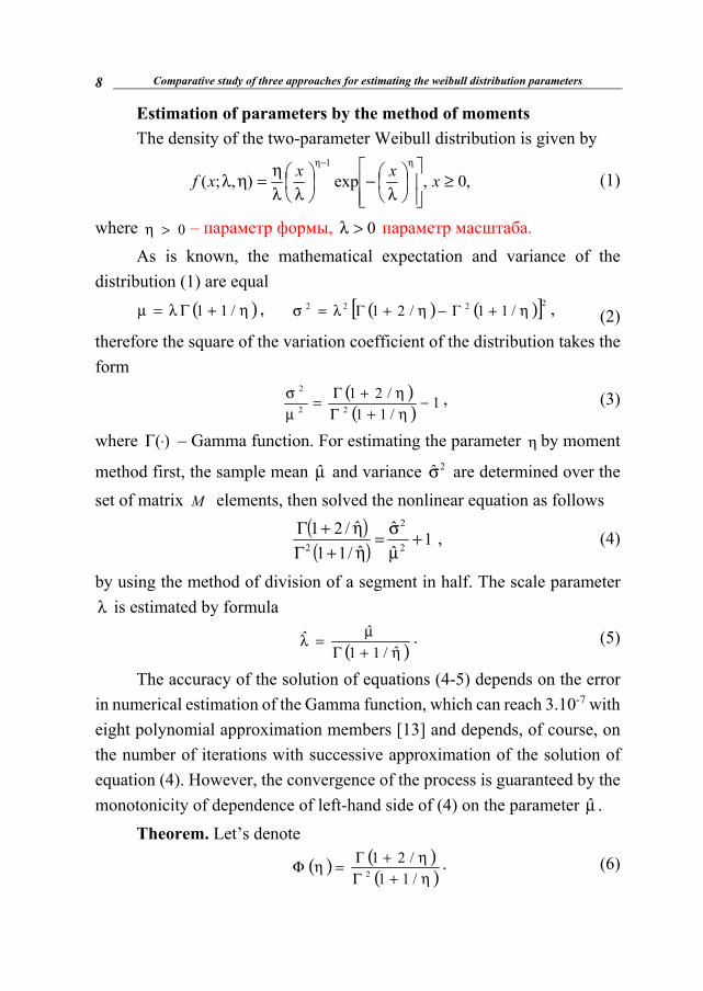
Estimation of parameters by the method of moments
The density of the two-parameter Weibull distribution is given by
,0,exp),;(1
≥
λ−
λλη=ηλ
η−η
xxxxf (1)
where 0>η – параметр формы, 0>λ параметр масштаба. As is known, the mathematical expectation and variance of the
distribution (1) are equal ( )η+Γλ=μ /11 , ( ) ( )[ ]2222 /11/21 η+Γ−η+Γλ=σ , (2)
therefore the square of the variation coefficient of the distribution takes the form
( )( ) 1
/11/21
22
2
−η+Γη+Γ=
μσ , (3)
where )(⋅Γ – Gamma function. For estimating the parameter η by moment
method first, the sample mean μ̂ and variance 2σ̂ are determined over the set of matrix M elements, then solved the nonlinear equation as follows
( )( ) 1
ˆˆ
ˆ/11ˆ/21
2
2
2 +μσ=
η+Γη+Γ , (4)
by using the method of division of a segment in half. The scale parameter λ is estimated by formula
( )η+Γ
μ=λˆ/11
ˆˆ . (5)
The accuracy of the solution of equations (4-5) depends on the error in numerical estimation of the Gamma function, which can reach 3.10-7 with eight polynomial approximation members [13] and depends, of course, on the number of iterations with successive approximation of the solution of equation (4). However, the convergence of the process is guaranteed by the monotonicity of dependence of left-hand side of (4) on the parameter μ̂ .
Theorem. Let’s denote
( ) ( )( )η+Γ
η+Γ=ηΦ/11/21
2. (6)

D. Asatryan 9
Then (6) decreases monotonically from η , i.e. 0)( <η
ηΦd
d for all 0>η .
Proof. After the logarithm of (6), we can obtain
( ) ( )η
η+Γη
+η
η+Γη
−=η
ηΦd
dd
dd
d /11ln2/21ln2)(ln22
. (7)
Let’s introduce the function dz
zdz )(ln)( Γ=ψ and use the well-
known property of this function ( ) zzz /1)(1 +ψ=+ψ , where the function
)( zψ is decreases monotonically [13]. Then note that the difference ( ) ( ) 2/)/2()/1(/21/11 η−ηψ−η+ηψ=η+ψ−η+ψ
increases monotonically, which, accordingly, leads to a monotonic decreasing of (6).
In Figure 1 a fragment of the plot of function ( )ηΦ is given.
Figure 1. A fragment of the plot of the function ( ).ηΦ
The proven property of monotonicity has one important «side effect» that allows us to accelerate the work of computer programs intended for ordering large arrays of images (or other objects) by the size of the Weibull

Comparative study of three approaches for estimating the weibull distribution parameters 10
distribution parameter without direct evaluation of the latter. For this it is sufficient to compare only the values of the coefficient of variation given in (3). A similar problem was considered in [9], in connection with the necessity of ordering an array of images by the magnitude of the blur.
Note that the results of numerical calculations for the above procedures, we use as «reference» for comparison with other methods of estimating the parameters of the Weibull distribution.
Estimation by the empirical formula using the coefficient of
variation In [14], the following simple empirical formula is given for estimating
the parameter of the Weibull distribution form in the form of a power function of the variation coefficient
086.1
ˆˆˆ
−
μσ=η . (8)
Calculations show that the accuracy provided by formula (8) is not very high on the average; therefore it can be used for relatively rough calculations. In this case, the accuracy of approximation by formula (8) is different for different intervals of variation of the form parameter η . For example, the relative accuracy of the formula is particularly low for values of 1.0≤η , and decreases, approaching 1% at 1.0=η . Further, by simple simulation of formula (8) and comparison with direct calculation results, it can be shown that the mean square error (MSE) in the interval has the values given in Table 1.
Table 1.
Mean square error of approximation of formula (8).
Range of definition of η 0.1 – 0.5 0.5 – 1.0 1.0 – 2.0 2.0 – 5.0
MSE of formula (8) 0.129 0.042 0.026 0.027
D. Asatryan 11
Thus, to estimate the form parameter of Weibull distribution within the limits of the accuracy indicated in Table 1, we can use formula (8).
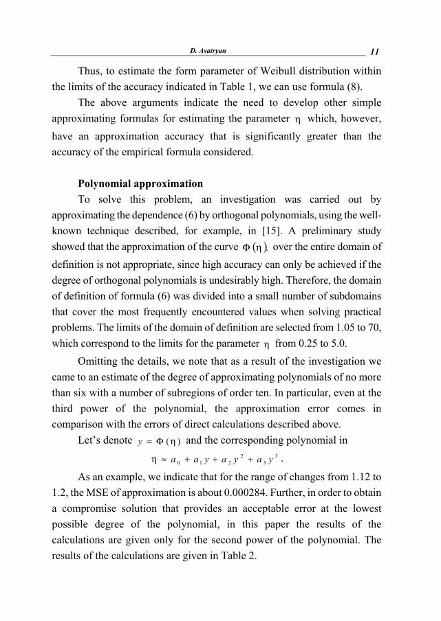
The above arguments indicate the need to develop other simple approximating formulas for estimating the parameter η which, however, have an approximation accuracy that is significantly greater than the accuracy of the empirical formula considered.
Polynomial approximation
To solve this problem, an investigation was carried out by approximating the dependence (6) by orthogonal polynomials, using the well-known technique described, for example, in [15]. A preliminary study showed that the approximation of the curve ( ).ηΦ over the entire domain of definition is not appropriate, since high accuracy can only be achieved if the degree of orthogonal polynomials is undesirably high. Therefore, the domain of definition of formula (6) was divided into a small number of subdomains that cover the most frequently encountered values when solving practical problems. The limits of the domain of definition are selected from 1.05 to 70, which correspond to the limits for the parameter η from 0.25 to 5.0.
Omitting the details, we note that as a result of the investigation we came to an estimate of the degree of approximating polynomials of no more than six with a number of subregions of order ten. In particular, even at the third power of the polynomial, the approximation error comes in comparison with the errors of direct calculations described above.
Let’s denote )(ηΦ=y and the corresponding polynomial in 3
32
210 yayayaa +++≈η .
As an example, we indicate that for the range of changes from 1.12 to 1.2, the MSE of approximation is about 0.000284. Further, in order to obtain a compromise solution that provides an acceptable error at the lowest possible degree of the polynomial, in this paper the results of the calculations are given only for the second power of the polynomial. The results of the calculations are given in Table 2.
Comparative study of three approaches for estimating the weibull distribution parameters 12
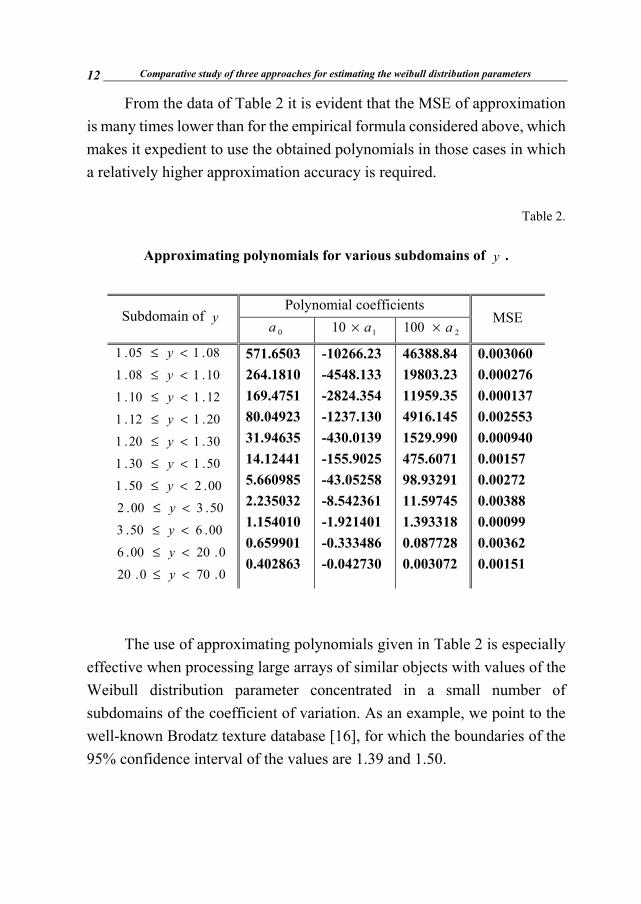
From the data of Table 2 it is evident that the MSE of approximation is many times lower than for the empirical formula considered above, which makes it expedient to use the obtained polynomials in those cases in which a relatively higher approximation accuracy is required.
Table 2.
Approximating polynomials for various subdomains of y .
Subdomain of y Polynomial coefficients
MSE 0a 110 a× 2100 a×
08.105.1 <≤ y
10.108.1 <≤ y
12.110.1 <≤ y
20.112.1 <≤ y
30.120.1 <≤ y
50.130.1 <≤ y
00.250.1 <≤ y
50.300.2 <≤ y
00.650.3 <≤ y
0.2000.6 <≤ y
0.700.20 <≤ y
571.6503
264.1810
169.4751
80.04923
31.94635
14.12441
5.660985
2.235032
1.154010
0.659901
0.402863
-10266.23
-4548.133
-2824.354
-1237.130
-430.0139
-155.9025
-43.05258
-8.542361
-1.921401
-0.333486
-0.042730
46388.84
19803.23
11959.35
4916.145
1529.990
475.6071
98.93291
11.59745
1.393318
0.087728
0.003072
0.003060
0.000276
0.000137
0.002553
0.000940
0.00157
0.00272
0.00388
0.00099
0.00362
0.00151
The use of approximating polynomials given in Table 2 is especially effective when processing large arrays of similar objects with values of the Weibull distribution parameter concentrated in a small number of subdomains of the coefficient of variation. As an example, we point to the well-known Brodatz texture database [16], for which the boundaries of the 95% confidence interval of the values are 1.39 and 1.50.

D. Asatryan 13
Conclusions
In this paper, we make a comparative analysis of the accuracy of three approximate methods for estimating the parameters of the Weibull distribution - a direct estimation method by solving the nonlinear equation of the moment method, the estimation method by the empirical formula representing the power function of the coefficient of variation and the method of approximation of the dependence of the form parameter estimate on the coefficient of variation in different intervals of its change. It is shown that the mean square error of approximation of the latter method by a polynomial of the second degree does not exceed 0.004. The research method allows, if necessary, to obtain more accurate approximation results, for which it is recommended to use polynomials of the third degree.
REFERENCES
1. Weibull W. Statistical Distribution of wide Applicability. Journal of Applied Mechanics, 18, 239–296, 1951.
2. Genc A., Erisoglu M., Pekgor A., Oturanc G., Hepbasli A. and Ulgen K. Estimation of wind power potential using Weibull distribution, Energy Sources 27, pp. 809–822, 2005.
3. Justus C., Hargraves W., Mikhall Amir and Graber Denise. Methods for Estimating Wind Speed Frequency Distributions. Journal of Applied Meteorology. V. 17, March, 350–353, 1978.
4. Lei Y. Evaluation of three methods for estimating the Weibull distribution parameters of Chinese pine (Pinus tabulaeformis). Journal of Forest Science, 54, (12): 566–571, 2008.
5. Teimouria Mahdi, Hoseinib Seyed M. and Nadarajahc Saralees. Comparison of estimation methods for theWeibull distribution. Statistics, Vol. 47, No. 1, 93–109, 2013.
6. Pobocikova Ivana, Sedliackova Zuzana, Šimon Ján. Comparative Study of Seven Methods for Estimating the Weibull Distribution

Comparative study of three approaches for estimating the weibull distribution parameters 14
Parameters for Wind Speed in Bratislava – Mlinska Dolina. Proceedings of 17th Conference on Applied Mathematics APLIMAT. PP. 840–852, 2018.
7. Kurbana Mehmet, Dokura Emrah and Ceyhanb Salim. A novel information geometry method for estimating parameters of the Weibull wind speed distribution. Proceedings of the Estonian Academy of Sciences, 67, 1, 39–49, 2018.
8. Yanulevskaya V. and Geusebroek J. Significance of the weibull distribution and its sub-models in natural image statistics, in Proceedings of the Fourth International Conference on Computer Vision Theory and Applications (VISAPP)], 1, 355–362, INSTICC Press, 2009.
9. Asatryan D. Image blur estimation using gradient field analysis [In Russian]. Computer Optics, 41(6), 957–962, 2017.
10. Timm Fabian and Barth Erhardt. Non-parametrric texture defect detection using Weibull features. Image Processing: Machine Vision Applications IV, volume 7877. Proceedings of SPIE. SPIE-IS&T. San Francisco, USA, 2011.
11. Asatryan D. Gradient-Based Technique for Image Structural Analysis and Applications. Computer Optics, 42(4), 111-111, 2018.
12. Plait Alan. The Weibull Distribution – With Tables. Industrial Quality Control. 19:17–26, 1962.
13. Справочник по специальным функциям. Под ред. М. Абрамовича и И. Стигана. М. «Наука», 1979.
14. Ramírez P., J. Carta A. Influence of the data sampling interval in the estimation of parameters of the Weibull wind speed probability density distribution a case study, Energy Conversion and Management, 46, 2419–2438, 2005.
15. Худсон Д. Статистика для физиков. М. «Мир», 1970. 16. http://www.ux.uis.no/~tranden/brodatz.html

D. Asatryan 15
СРАВНИТЕЛЬНОЕ ИССЛЕДОВАНИЕ ТРЕХ ПОДХОДОВ
К ОЦЕНИВАНИЮ ПАРАМЕТРОВ РАСПРЕДЕЛЕНИЯ ВЕЙБУЛЛА
Д. Асатрян
АННОТАЦИЯ
Распределение Вейбулла часто используется при моделировании вы-
живания, надежности, скорости ветра, свойств цифровых изображений и других данных. Существуют множество распространенных методов оцени-вания параметров распределения Вейбулла. Некоторые из них основаны на оценивание методом моментов (ОММ) и его модификациями. Однако, нес-мотря на алгоритмическую простоту применяемых процедур, возникла необ-ходимость создания более быстродействующих методов, позволяющих из-бежать объемных вычислений, связанных с оценкой Гамма фунции и с про-цедурой последовательных приближений. В настоящей статье на основе ана-лиза данных и моделирования изучаются и сравниваются следующие три ме-тода оценивания: прямой метод оценивания путем решения нелинейных уравнений ОММ, метод оценивания при помощи эмпирической формулы, представляющей собой степенную функцию от коэффициента вариации и метод полиномиальной аппрксимации зависимости оценки параметра фор-мы от коэффициента вариации в различных интервалах его значений.
Ключевые слова: распределение Вейбулла, оценивание параметров, метод моментов, полиномиальная аппроксимация, ошибка аппроксимации.
ՎԵՅԲՈՒԼԻ ԲԱՇԽՄԱՆ ՊԱՐԱՄԵՏՐԵՐԻ ԳՆԱՀԱՏՄԱՆ ԵՐԵՔ ՄՈՏԵՑՈՒՄՆԵՐԻ ՀԱՄԵՄԱՏԱԿԱՆ ՀԵՏԱԶՈՏՈՒԹՅՈՒՆ
Դ. Ասատրյան
ԱՄՓՈՓՈՒՄ
Վեյբուլի բաշխումը հաճախ օգտագործվում է որպես survival, հուսա-
լիության, քամու արագության, թվայնացված պատկերների հատկություն-ների և այլ տվյալների վիճակագրական մոդել: Առաջարկվել են և լայնորեն

Comparative study of three approaches for estimating the weibull distribution parameters 16
կիրառվում են Վեյբուլի բաշխման պարամետրերի գնահատման մի շարք մեթոդներ: Դրանց մի մասը հենված է պարամետրերի գնահատման՝ մոմենտների մեթոդի (ՄՄԳ) և դրա ձևափոխումների վրա: Սակայն, չնայած համապատասխան ընթացակարգերի ալգորիթմական պարզությանը, անհրաժեշտություն է առաջացել ավելի արագագործ մեթոդներ ստեղծելու, որպեսզի խուսափեն Գամմա ֆունկցիայի և հաջորդական մոտեցումների եղանակի իրագործման համար կատարվող ծավալուն հաշվարկներից: Սույն հոդվածում տվյալների վերլուծության և մոդելավորման միջոցով հետազոտվել են պարամետրերի գնահատման հետևյալ երեք մեթոդները. ՄՄԳ ոչ գծային հավասարումների լուծման միջոցով գնահատման ուղիղ մեթոդը, փոփոխականության գործակցից աստիճանական ֆունկցիայի տեսքով էմպիրիկ բանաձևի օգնությամբ գնահատման մեթոդը և ձևի պարամետրի՝ փոփոխականության գործակցից կախվածության բազմանդամային մոտարկման մեթոդը գործակցի արժեքների տարբեր միջակայքերի համար:
Հիմնաբառեր` Վեյբուլի բաշխում, պարամետրերի գնահատում, մո-մենտների մեթոդ, բազմանդամային մոտարկում, մոտարկման սխալանք:

17
УДК 004.04
ON AN APPROACH FOR SUPPORTING QUERIES
BUILT IN NATURAL LANGUAGE
N. Hovsepyan
Information Technologies Educational and Research Center,
Yerevan State University
ABSTRACT
Generating queries for databases from natural language is a known problem. With the increasing amount of data in the world it is important to give people who do not have the knowledge of SQL or other query languages access to these data. To solve the problem of generating SQL queries from natural language, we consider two level neural networks. The first level for generation of the main components (aggregation function, column name, conditions) and the second onefor formulation of the final query from the main components. In this paper, we used bidirectional recurrent neural network with fully connected layers and achieved higher accuracy than all known results.
Keywords: SQL, natural language, machine learning, neural networks, deep learning
1. Introduction
Nowadays, almost every business data is stored in databases, whichrequires knowledge of query language in order to access such data.
Вестник РАУ № 2, 2018, 17-26
On an approach for supporting queries built in natural language 18
Generation of SQL queries from natural language will significantly ease the problem of accessing data. Considered work is aimed to suggest a solution to the problem, hence making the data-processing workflow simpler.
One of the successful works using WikiSQL dataset [9] for training and testing has been published in 2017 [8]. The result was 59.4% accuracy on test set, exceeding the previous best result (35.9%) by over 20%. Another work [1] has been published by Microsoft Research group in November 2017 with 66.8% accuracy using deep sequence to sequence model with some attention mechanisms and extensions. Also, good result was achieved in November 2017 [10] with 68% accuracy, which was the state of the art method before our results. All previous works [2] use machine learning models with some extensions and modifications.
2. Dataset
In this paper we have used the WikiSQL dataset which has been manually collected from Wikipedia database tables. It contains more than 80 thousand examples of natural language questions and the corresponding SQL queries distributed across 26 thousand tables. The dataset is splitted into two groups, one for training 80% and the other for testing 20%.
The WikiSQL data collection queries are applied for a single table. The structure of the query is the following:
select aggregation | name
from table
where predicates.
There are also other data collections (e.g. SENLIDB), but unlike
WikiSQL, they are small and have only one table.
3. Model description
In this paper, we have implemented relatively simpler models and have achieved higher accuracy, compared to previous works.

N. Hovsepyan 19
We use two level neural networks. The first level networks are used to predict the aggregation, column name and conditions from the natural language query. The second levelis based on the results of the first level and constructs the final SQL query.
The division of the problem into two levels is justified, because each of them can be processed and solved independently of the other. Therefore, this division gave us the opportunity to train relatively simple models and by combining the results achieve high accuracy.
Since the query structure in the WikiSQL dataset is fixed and applied for a single table, machine learning models which should generate these queries using the main components will quickly overfit. Therefore, weconstructed a program for generating SQL queries, which will replace second level network.
For future work, we plan to find more datasets that cover a wider range of complex queries specifically with use of multiple tables, and train generalized neural networks to solve the second level problem too.
3.1. Aggregation prediction
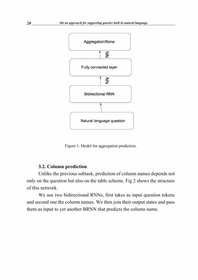
First subtask of first level is aggregation function prediction. We assume aggregation function can be predicted from the natural language question only. The model which we use for this subtask shown in Figure 1.
We use bidirectional RNN on top of the question tokens, after the final state output of the RNN there is fully connected layer and output with six neurons. We interpret this as six class classification problem, where classes are {NONE, SUM,AVG,MAX,MIN,COUNT} (NONE if no aggregation needed). Loss function is categorical cross-entropy (CCE), where q is probability distribution, p is «true» distribution:
, = − log
On an approach for supporting queries built in natural language 20
Figure 1. Model for aggregation prediction.
3.2. Column prediction
Unlike the previous subtask, prediction of column names depends not only on the question but also on the table scheme. Fig 2 shows the structure of this network.
We use two bidirectional RNNs, first takes as input question tokens and second one the column names. We then join their output states and pass them as input to yet another BRNN that predicts the column name.

N. Hovsepyan 21
Figure 2. Model for column prediction.
3.3. Conditions prediction
For the conditions prediction subtask, we use the same model as in previous task. Unlike previous subtask which needs to predict only one column name in the output, this one should predict one or more simple conditions joined with logical operations. Example of dataset element:
table schema: {«Round», «Grand Prix», «Pole Position», «Fastest
Lap», «Winning Driver», «Winning Constructor», «Report»} question: «How many Grand Prix were the winning constructor
Benetton - Ford and the pole position was Michael Schumacher?» For this natural language question, we need to have two simple conditions, first «Winning Constructor» need to be equal to «Benetton – Ford» and second «Pole Position» need to be equal to «Michael Schumacher» joined with logical and operation.

On an approach for supporting queries built in natural language 22
3.4. Query generation
Previous models are solving the first level subtasks of predicting main components of the query. Now it remains to create the final SQL query string using these results. As mentioned above, WikiSQL has fixed structure of SQL queries which allows us to build a program for generating final queries.
Figure 3. Two level neural networks.
4. Experiments
We use tensorflow [5] python library for our experiments. Also, we have used GloVe pre-trained word vectors [3] to get real vector for each word of natural language question and used only this vector representation. All bidirectional RNNs have 128 hidden units. We used the ADAM optimizer for training our neural networks.
As shown in Table 1, we achieve 87.6% accuracy in aggregation prediction subtask, 89.8% in column prediction. Condition prediction task is more complex compared to previous ones, because in this problem part

N. Hovsepyan 23
of the queries have multiple conditions. On test set for this subtask we reach 72.3% accuracy.
Table 1.
First level network’s results.
Subtask name Accuracy on test set
Aggregation prediction 87.6%
Column prediction 89.8%
Conditions prediction 68.7%
The whole two level neural networks solution reaches 68.7%
accuracy on test set, which exceeds all the known results before this work and is a new state of the art result.
5. Conclusion
In this paper we described a new approach which allowed us to get new state of the art result with use of simple machine learning models. Division of the problem resulted in easier subproblems and our two-level approach solves the problem better. Two level neural networks approach makes easier to generate final query with use of already solved subtasks of the first level. Next steps for this work is to use various complex and suggested models from previous works for the subtasks and levels of this model, keeping our approach which can lead to even better results. Also, we can extend WikiSQL and add SQL queries which have more complex structures to train and generalize the second part of the problem.

On an approach for supporting queries built in natural language 24
REFERENCES 1. Chenglong Wang, Marc Brockschmidt and Rishabh Singh. POINTING
OUT SQL QUERIES FROM TEXT. 2017 https://www.microsoft.com/en-us/research/wp- content/uploads/2017/11/nl2prog.pdf
2. Androutsopoulos, G.D. Ritchie and P.Thanisch. Natural language interfaces to databases an introduction. 1995.
3. Jeffrey Pennington, Richard Socher and Christopher D. Manning. Glove: Global vectors for word representation. In EMNLP, 2014.
4. Dong Li, Lapata Mirella. Coarse-to-Fine Decoding for Neural Semantic Parsing. CoRR, abs/1805.04793, 2018.
https://arxiv.org/abs/1805.04793 5. https://arxiv.org/abs/1803.02400 6. M. Abadi, A. Agarwal, P. Barham, E. Brevdo, Z. Chen, C. Citro,
G.S. Corrado, A. Davis, J. Dean,. Devin, S. Ghemawat, I. Goodfellow,
A. Harp, G. Irving, M. Isard, Y. Jia, R. Jozefowicz, L. Kaiser, M.
Kudlur, J. Levenberg, D. Mane, R. Monga, S. Moore, D. Murray, C.
Olah, M. Schuster, J. Shlens, B. Steiner, I. Sutskever, K. Talwar, P.
Tucker, V. Vanhoucke, V. Vasudevan, F. Viegas, 0. Vinyals, P. Warden,
M. Wattenberg, M. Wicke, Y. Yu, and X. Zheng. Tensor Flow: Large-scale machine learning on heterogeneous systems, 2015. URL https://www.tensorflow.org/. Software available from tensorflow.org.
7. Po-Sen Huang, Chenglong Wang, Rishabh Singh, Wen-tau Yih,
Xiaodong He. Natural Language to Structured Query Generation via Meta-Learning. CoRR, abs/1803.02400, 2018.
https://arxiv.org/abs/1803.02400. 8. Tao Yu, Zifan Li, Zilin Zhang, Rui Zhang, DragomirRadev. TypeSQL:
Knowledge-based Type-Aware Neural Text-to-SQL Generation. CoRR, abs/1804.09769, 2018. https://arxiv.org/abs/1804.09769
N. Hovsepyan 25
9. Victor Zhong, Caiming Xiong and Richard Socher. Seq2sql: Generating structured queries from natural language using reinforcement learning. arXiv preprint arXiv:1709.00103, 2017
10. WikiSQL dataset, https://github.com/salesforce/WikiSQL. 11. X. Xu, C. Liu and D. Song. Sqlnet: Generating structured queries from
natural language without reinforcement learning. CoRR, abs/1711.04436, 2017. URL http://arxiv.org/abs/1711.04436.
ОБ ОДНОМ ПОДХОДЕ К ПОДДЕРЖКЕ ЗАПРОСОВ,
ПОСТРОЕННЫХ НА ЕСТЕСТВЕННОМ ЯЗЫКЕ
Н. Овсепян
АННОТАЦИЯ
Генерация запросов для базы данных с помощью естественных языков является известной проблемой. Учитывая рост объема данных, важно предоставить возможность доступа к этим данным тем людям, которые не имеют знания SQL или других языков запросов. Для решения проблем генерации SQL запросов из естественного языка, мы рассматриваем двухуровневые нейронные сети. Первый уровень выполняет генерацию основных компонентов (функции агрегации, имена столбцов, условия и т.д.). Функцией второго уровня является составление заключительного запроса, используя сгенерированные основные компоненты. В данной работе мы использовали двухсторонние рекуррентные нейронные сети с полностью соединенными слоями и достигли более высокой точности по сравнению с известными результатами.

On an approach for supporting queries built in natural language 26
ԲՆԱԿԱՆ ԼԵԶՎՈՎ ԿԱՌՈՒՑՎԱԾ ՀԱՐՑՈՒՄՆԵՐԻ
ԱՋԱԿՑՄԱՆ ՄԻ ՄՈՏԵՑՄԱՆ ՄԱՍԻՆ
Ն. Հովսեփյան
ԱՄՓՈՓՈՒՄ
Տվյալների բազաների համար բնական լեզվից հարցումների գեներա-
ցիան բավականին հայտնի խնդիր է։ Տվյալների աճին զուգընթաց շատ կա-
րևոր է ապահովել այդպիսի տվյալների հասանելիությունը այն մարդկանց
համար, ովքեր չեն տիրապետում SQL կամ այլ հարցումների լեզուների։
Բնական լեզվից հարցումներ գեներացնելու խնդիրը լուծելու համար մենք
դիտարկում ենք նեյրոնային ցանցեր՝ բաղկացած երկու մակարդակից։
Առաջին մակարդակը նախատեսված է հիմնական մասերի գեներացիայի
համար (ագրեգատային ֆունկցիաներ, սյունակի անուն, պայմաններ), իսկ
երկրորդ մակարդակը՝ հիմնական մասերը օգտագործելով վերջնական
հարցումը կառուցելու համար։ Այս հոդվածում մենք օգտագործել ենք
երկկողմանի ռեկուրենտ նեյրոնային ցանցեր, լրիվ կապակցված շերտերով
և հասել ավելի բարձր ճշգրտության, քան մինչև այս հայտնի արդյունք-
ներում։
Вестник РАУ № 2, 2018, 27-36 27
UDC 621.311
INCREASING THE SPEED OF DETECTING
OBJECTS IN THE VIDEO BY THE OPTIMIZATION
OF THE PROCESS
D. Simonyan
RA NAS IIAP
ABSTRACT
To solve the task of ensuring the safety of the area in the sphere of surveillance, the quick detection of the objects is of utmost importance. The methods applied at present ensure certain speed, but our goal is to develop a more quick-operating method, at the same time, ensuring the satisfactory quality of detection by which it will be possible to accurately determine the type of the objects.
Keywords: image processing, object detection and recognition, background subtraction, performance, optimization, image pyramid, Open CV.
Introduction. Nowadays, object detection and recognition in the video is widely used in many spheres. The existing methods of detection and recognition can be divided into two main groups: methods based on "frame difference" and methods of background subtraction in the image which works by applying the calculation of the absolute shift difference

Increasing the speed of detecting objects in the video by the optimization of the process 28
between the frames, using the XOR bit comparison between the images. In the background subtraction method, as a result of subtracting the background from the current image, we will obtain the complete view of the objects,existing on the image which is difficult to implement by the method based on the frame difference. Thus, in the process of the object detection and recognition, the background subtraction is preferable. But as a consequence of using the latter, a number of problems arise, thus for instance, the presence of false targets in the image, as well as a difference of the light intensity between the background and current frames, depending on the climatic changes. The solution of the problems have been obtained by the method [1] (which is a modification of a background subtraction method in the image), and by that proposed in [2].
A task has been set to obtain a more quick-operating version of the method of the background subtraction in the image, at the same time ensuring the accuracy of determining the type of the object. For increasing the speed of the object detection (and, at the same time, maintaining the quality), a modification of the background subtraction method has been performed.
The following three stages of the task have been implemented: 1. Construction of the image pyramid. The sphere of image analysis
includes the theory of the image pyramid, which is very frequently used to reduce the noise in the image [3]. In this stage, the image pyramid has been constructed based on the following principle:
The base of the pyramid is the original frame taken from the video, which is subjected to the ∝ −operation,after which,the image is reduced several times by the coefficient (Fig. 1). This allows to significantly reduce the noise in the image and by means of frame subtraction, compare the small images while comparing the whole images, which, in its turn, will favour the speed of the algorithm.

D. Simonyan 29
Figure 1. The image pyramid.
The base of the pyramid obtained as a result of matrix modification of the current image of the video is the matrix ( , ):
( , ) = ∝ ( , ) , = 2 , (1)
while the view f (x, y) of the matrix obtained as a result of the image reduction, i.e. the passage from one layer of the pyramid onto the other is calculated by the following formula: ( , ) = ( , ), = 1, (2)
where ( , ) is the matrix of the current image of the video; ( , )– the zero layer of the pyramid; ∝- the coefficient of actions applied on the image

Increasing the speed of detecting objects in the video by the optimization of the process 30
(grayscale, blur); – the number of the pyramid layers; – the reduction coefficient of the image dimensions.
As a result of constructing the pyramid, we will obtain the small analogue of the original frame and name it ( , ).
2. Grid construction in the last layer of the pyramid. At video surveillance, the small objects in the image are of no interest. The user has an opportunity to define the possible minimal size of the object. The object
smaller than the size × defined in the background will be neglected by
the system. After defining the size, the grid is constructed according to the minimal size of the mentioned object in the following way.
As there is conformity between the obtained ( , ) and the ( , ) original images, we can distribute the pixels of the ( , ) image sparsely on the original frame and obtain a grid (Fig. 2.). Thus, each point of the grid is a pixel of the image ( , ).
Figure 2. Construction of the grid in the image.

D. Simonyan 31
3. Detection of the objects (description of the XOR bit comparison
algorithm). Mentioned XOR bit comparison algorithm is the following: Each point of the grid is consideredsuccessively. If the colour value
{R,G,B} of the grid point differs from the background, the 3x3-size matrix is placed on the corresponding pixel of the grid point in the original frame. From the colour difference, it is assumed that the given point is the object pixel. Then, 8 neighbouring points are analysed in the original frame, which are also compared with the background image. That is, the algorithm passes through each point of the sparse grid until it comes across a colour difference where the object is.
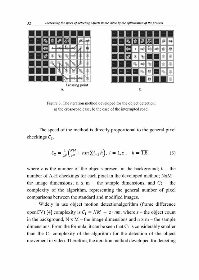
In Fig. 3, each square is one pixel in the original frame, while the object is expressed by white squares. Passing through the grid points, the algorithm reaches the object pixel. Thus for instance, let us consider the centre of the square marked in red in Fig. 3. After that we pass onto checking the neighbouring pixels of the corresponding point in the original frame. In particular, seeing that points A, B, C, G and H are not points of the object, we mark them in black in the output image, while D, E, F – in white. Then we place the matrix on D and check the neighbouring pixels that have not yet been checked. Then we move in the direction of D1, then D2 and so on up to Dn (Fig. 3a). In this way, we complete all the pixels of the object, obtaining its full view (in the output image). In Fig. 3b, the case of the interrupted sequence is introduced when the algorithm for detecting the object pixels, moving in the direction of D, does not complete the process with a single iteration and, in that case, the second iteration starts and continues to move in the direction of E, ending the process in the point En.
After expandingwithin the original frame and detecting all the pixels of the object, we will return to the grid and continue the object search.
Increasing the speed of detecting objects in the video by the optimization of the process 32
Figure 3. The iteration method developed for the object detection: a) the cross-road case; b) the case of the interrupted road.
The speed of the method is directly proportional to the general pixel checkings . = + ∑ ℎ , = 1, , ℎ = 1,8 (3)
where z is the number of the objects present in the background; h – the number of A-H checkings for each pixel in the developed method; NxM – the image dimensions; n x m – the sample dimensions, and C2 – the complexity of the algorithm, representing the general number of pixel comparisons between the standard and modified images.
Widely in use object motion detectionalgorithm (frame difference openCV) [4] complexity is = + z ∙ nm, where z – the object count in the background, N x M – the image dimensions and n x m – the sample dimensions. From the formula, it can be seen that C2 is considerably smaller than the C1 complexity of the algorithm for the detection of the object movement in video. Therefore, the iteration method developed for detecting
D. Simonyan 33
the object is speedy in comparison with the previous methods, which is also proved by experiments.
The results of the experiments. Numerous experiments have been made for the developed method (for about 5000 frames of 7 different video materials). As a comparison method, the method of frame difference Open CV for the object movement detection in the video widely used in the given sphere has been selected.
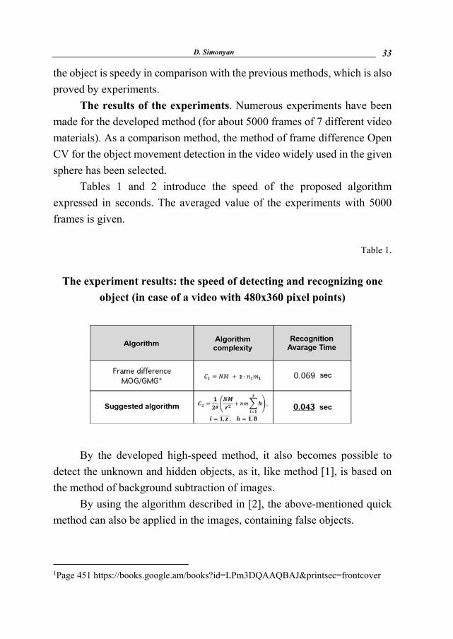
Tables 1 and 2 introduce the speed of the proposed algorithm expressed in seconds. The averaged value of the experiments with 5000 frames is given.
Table 1.
The experiment results: the speed of detecting and recognizing one
object (in case of a video with 480x360 pixel points)
1 By the developed high-speed method, it also becomes possible to
detect the unknown and hidden objects, as it, like method [1], is based on the method of background subtraction of images.
By using the algorithm described in [2], the above-mentioned quick method can also be applied in the images, containing false objects.
1Page 451 https://books.google.am/books?id=LPm3DQAAQBAJ&printsec=frontcover

Increasing the speed of detecting objects in the video by the optimization of the process 34
Table 2. The experiment results: the speed of the object detection
in case of varying pixel points
Conclusion
1. A speedy version of the object detection in the video has been developed due to the modification of the background subtraction method. It detects the objects hidden in the background (which are not visible with naked eye) with satisfactory accuracy. At that, the object may be both stationary and in motion.
2. The developed method detects the objects in the image, taking into account the possible change of light and climate in the course of the video surveillance. The types of the detected objects in the image are not limited by this method.
3. Experiments have been carried out which have confirmed the quick operation of the algorithm as compared with the other existing algorithms.
4. Together with the increase in the detection speed, the accuracy of determining the object type has been maintained.
5. The object detection and recognition by the developed method is also applicable for the images, containing false targets.
D. Simonyan 35
REFERENCES
1. Simonyan R. Hidden and Unknown Object Detection in Video, In International Journal of New Technology and Research (IJNTR) Volume 2, Issue 11. PP. 22–25, November 2016.
2. Simonyan R., Simonyan D. Detection and ignorance method of false targets during object detection. In Computer Science and Information Technologies (CSIT) Conference 2017. PP. 372–375.
3. Dollár P., Appel R., Belongie S., Perona P. Fast Feature Pyramids for Object Detection. In IEEE Transactions on Pattern Analysis and Machine Intelligence, Volume 36, Issue 8. PP. 1532–1545, 2014.
4. Kahler A. and Bradski G. Book title. "Learning OpenCV 3: Computer Vision in C++ with the OpenCV Library". PP. 451–491.
5. Simonyan R. Object Recognition Using Template Based Matching Method. In Transactions of IIAP of NAS of RA, Mathematical Problems of Computer Science, Volume 49, 2018.
6. Simonyan R. Object Distance Detection from Surveillance Cameras. International Journal of Science and Engineering Investigations, Volume 7, Issue 74. PP. 104–106, March 2018.
7. Simonyan R. Recognized Objects Visualization on Maps. International Journal of Science and Engineering Investigations, Volume 7, Issue 75. PP. 104–108, April 2018.
8. Cinbis R., Sclaroff S. Contextual Object Detection using Set-based Classification. 2012, PP. 15–64.
9. Swaroop P., Sharma N. An Overview of Various Template Matching ethodologies in Image Processing. In International Journal of Computer Applications (0975–887), Volume 153. No 10. PP. 8–14, November 2016.

Increasing the speed of detecting objects in the video by the optimization of the process 36
ПОВЫШЕНИЕ СКОРОСТИ ОБНАРУЖЕНИЯ ОБЪЕКТОВ В ВИДЕОПОТОКЕ ПУТЕМ ОПТИМИЗАЦИИ ПРОЦЕССА
Д.А. Симонян
АННОТАЦИЯ
В сфере видеонаблюдения для реализации проблем сохранения безо-пасности территории особенно важно быстрое обнаружение объектов. При-меняемые ныне методы обеспечивают определенное быстродействие, одна-ко нашей целью является разработка более быстродействующего метода для обеспечивания удовлетворительного качества обнаружения, что позволит более корректно определить типы объектов.
Ключевые слова: обработка изображения, обнаружение и распозна-вание объектов, метод фоновой фильтрации, оптимизация, пирамида изобра-жений, Open CV.
ՏԵՍԱՇԱՐՈՒՄ ՕԲՅԵԿՏՆԵՐԻ ՀԱՅՏՆԱԲԵՐՄԱՆ ԳՈՐԾԸՆԹԱՑԻ ԱՐԱԳՈՒԹՅԱՆ ԲԱՐՁՐԱՑՈՒՄԸ ՕՊՏԻՄԱԼԱՑՄԱՆ ՄԻՋՈՑՈՎ
Դ.Ա. Սիմոնյան
ԱՄՓՈՓՈՒՄ
Տեսահսկման ոլորտում տարածքի անվտանգության պահպանման
խնդիրը իրագործելու համար առավել կարևոր է օբյեկտների արագ հայտ-
նաբերումը: Ներկայումս կիրառություն գտած մեթոդները ապահովում են
որոշակի արագագործություն, սակայն մեր նպատակն է մշակել առավել
արագագործ մեթոդ, միաժամանակ ապահովելով հայտնաբերման բավա-
րար որակ, որով հնարավոր կլինի ճշգրտորեն որոշել օբյեկտների տեսակը:
Հիմնաբառեր՝ պատկերների մշակումը, օբյեկտների հայտնաբերում և
ճանաչում, ֆոնային զատման մեթոդ, արագագործություն, օպտիմալացում,
պատկերների բուրգ:

Вестник РАУ № 2, 2018, 37-54 37
УДК 517.968.4
О РАЗРЕШИМОСТИ ОДНОГО КЛАССА
НЕЛИНЕЙНЫХ ПСЕВДОДИФФЕРЕНЦИАЛЬНЫХ
УРАВНЕНИЙ НА ВСЕЙ ПРЯМОЙ
Х.А. Хачатрян,1 Э.А. Андреасян2
1Институт математики НАН Армении 2Ереванский государственный университет
АННОТАЦИЯ
Данная научная статья посвящена вопросам разрешимости в пространстве Соболева (ℝ ) одного класса псевдодифферен-циальных уравнений. При определенных условиях на нелинейную часть доказано, что рассматриваемое уравнение имеет нечетное ре-шение ∈ (ℝ ) с определенным поведением на бесконечности и удовлетворяющим условию (0) = 0.
Ключевые слова: нетривиальное нечетное решение, прост-ранство Соболева, монотонность, итерации, асимптотика решения.
1. Введение
Пусть ( ) − определенная на ℝ нечетная и непрерывная функ-ция, удовлетворяющая следующим условиям: ( ) ( ) = , причем число > 0является первым положительным корнем уравнения ( ) = , ( ) существуют числа > 1 и ∈ (0, ) такие, что ( ) ≥ , ∈ (0, ),
О разрешимости одного класса нелинейных псевдодифференциальных уравнений... 38( ) функция ( ) возрастает на отрезке [0, ]. Рассмотрим следующую граничную задачу: − ( ) + ( ) = ( )( ) , ∈ ℝ,(1)(0) = 0, (±∞) ≔ lim→± ( ) = ± (2)
относительно искомой вещественной функции ( ), где – продол-жение на (ℝ) ≔ ( ) ∶ ( ) ∈ (ℝ), = 0,1,2, ∈ ℝ
оператора, порожденного дифференциальной формой . Задача (1) − (2) эквивалентна следующей граничной задачи для
интегро-дифференциального уравнения вида: − ( ) + ( ) = ( − ) ( ) , ∈ ℝ,(3)(0) = 0, (±∞) = lim→± ( ) = ± , ∈ (ℝ),(4)
где = √ , ( ) = √4 , ∈ ℝ.(5) Задача возникает в − адической теории струны (см. [1] − [3]).
Соответствующее интегральное уравнение без производной второго порядка при определенных Qизучено в работах [1]и[3].
Соответствующая граничная задача на полуоси при более сильных ограничениях на нелинейность исследована в работах [4] −[7].
Исходя именно из физических соображений, будем искать нечет-ные решения для граничной задачи (3) − (4) (см. [1] − [3]).
Прямой проверкой можно убедиться, что если функция ( ) яв-ляется решением следующей граничной задачи на полуоси:

Х.А. Хачатрян, Э.А. Андреасян 39
− ( ) + ( ) = ( − ) − ( + ) ( ) , ∈ ℝ , (6)(0) = 0, (+∞) = , ∈ (ℝ ),(7)
то нечетное продолжение функции ( )наℝ ≡ (−∞, 0): ( ) = ( ),если ≥ 0,− (− ),если < 0 будет решением граничной задачи (3) − (4)и, следовательно, перво-начальной задачи (1) − (2).
2. Сведение задачи ( ) − ( ) к интегральному уравнению.
Априорные оценки
Нетрудно проверить, что в (ℝ )задача (6) − (7) эквива-лентна следующей задаче: ( ) + ( ) =
= ( ) ( − ) − ( + ) ( ) , ∈ ℝ , (8) с граничными условиями (7). Обозначим через ( ) = ( ) + ( ), ∈ ℝ .(9)
Тогда с учетом (7) и(9) приходим к следующему нелинейному интегральному уравнению: ( ) = ( ) ( − ) − ( + )
( ) ( ) , ∈ ℝ (10) относительнофункции , удовлетворяющей условиям:
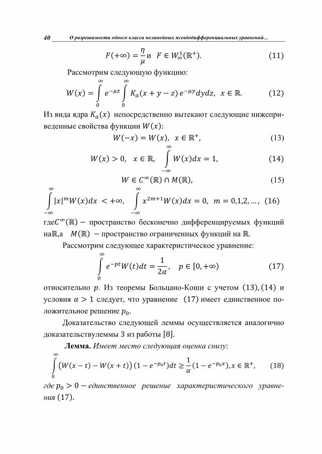
О разрешимости одного класса нелинейных псевдодифференциальных уравнений... 40 (+∞) = и ∈ (ℝ ).(11) Рассмотрим следующую функцию: ( ) = ( + − ) , ∈ ℝ.(12) Из вида ядра ( )непосредственно вытекают следующие нижепри-веденные свойства функции ( ): (− ) = ( ), ∈ ℝ , (13) ( ) > 0, ∈ ℝ, ( ) = 1,(14) ∈ (ℝ) ∩ (ℝ), (15) | | ( ) < +∞, ( ) = 0, = 0,1,2,… ,(16) где (ℝ) − пространство бесконечно дифференцируемых функций наℝ,а (ℝ) −пространство ограниченных функций на ℝ.
Рассмотрим следующее характеристическое уравнение: ( ) = 12 , ∈ [0, +∞)(17) относительно . Из теоремы Больцано-Коши с учетом (13), (14) и условия > 1 следует, что уравнение (17)имеет единственное по-ложительное решение .
Доказательство следующей леммы осуществляется аналогично доказательствулеммы 3 из работы [8].
Лемма. Имеет место следующая оценка снизу: ( − ) − ( + ) (1 − ) ≥ 1 (1 − ), ∈ ℝ , (18) где > 0 −единственное решение характеристического уравне-ния(17).

Х.А. Хачатрян, Э.А. Андреасян 41
3. Последовательные приближения для интегрального урав-
нения ( ) Рассмотрим для уравнения (10) следующие последовательные
приближения: ( ) = ( ) ( − ) − ( + )
( ) ( ) , ∈ ℝ ,(19) ( ) ≔ , = 0,1,2, … , ∈ ℝ .
Из определения , с учетом монотонности на [0, ] и(5) при = 0 имеем:
0 ≤ ( ) ≤ ( ) ( − ) − ( + ) ≤≤ ( ) ( − ) ≤ ( ) =
= ( ) ( ) = = ( ). Предполагая, что для некоторого натурального ( ) ≥ 0и ( ) ≤ ( ), ∈ ℝ (20) и используя монотонность функции на [0, ], из (19), получим: ( ) ≤ ( ) ( − )
− ( + ) ( ) ( ) == ( ),

О разрешимости одного класса нелинейных псевдодифференциальных уравнений... 42 ( ) ≥ 0, ∈ ℝ . Теперь докажем, что для любого натурального имеет место
следующая оценка снизу: ( ) ≥ (1 − ), ∈ ℝ .(21) В случае = 0 неравенство (21) непосредственно следует из включе-ния ∈ (0, )и определения нулевого приближения. Предполагая, что (21)имеет место при некотором ∈ ℕ и используя монотонность функции , а также неравенство ( ), из (19, ) будем иметь: ( ) ≥ ( ) ( − ) − ( + )
( )(1− ) .(22) Так как 0 ≤ ( − ) − ( + ) ( )(1 − ) ≤
≤ ( − ) − ( + ) ( ) ≤
≤ ( − ) − ( + ) ≤ ( − ) ≤ = , то из (22), (18), (а ) с учетом теоремы Фубини (см.[9])имеем: ( ) ≥ ≥ ( ) ( − ) − ( + ) ( )(1 − ) =
= ( − ) − ( + ) (1 − ) ≥

Х.А. Хачатрян, Э.А. Андреасян 43≥ 1 (1 − ) = (1 − ). Итак, оценки (21) доказаны.
Из непрерывности функции и (19)следует, что ∈ (ℝ ),= 0,1,2,…. Записывая итерации(19) следующим образом: ( ) = ( ) ( + − − ) −
− ( + + ) ( ) ( ) ,
( ) = , = 0,1,2, … , ∈ ℝ
и используя монотонность ядра ( ) и функции , индукцией по , можно доказать, что ( ) ↑ по наℝ , = 0,1,2, ….(23)
Следовательно, последовательность ( ) непрерывных функций имеет поточечный предел, когда → ∞: lim→ ( ) = ( ), который является решением уравнения (10)в силу теоремы Б. Леви (см.[9]), причем (1 − ) ≤ ( ) ≤ , ∈ ℝ ,(24) ( ) ↑ по наℝ .(25)
Из непрерывности ядра и функции с учетом (10) следует непрерывность предельной функции ( ). Так как ∈ (ℝ ), то опять, используя непрерывность ядра и функции ,заключаем, что ( − ) − ( + ) ( ) ( )
∈ (ℝ ) ∩ (ℝ ).(26)

О разрешимости одного класса нелинейных псевдодифференциальных уравнений... 44
Следовательно,
( ) ( − )− ( + ) ( ) ( ) ∈ (ℝ ).(27)
Таким образом, с учетом (27)и (10) заключаем, что ∈(ℝ ). Из свойств функции ( ) следует, что существует lim→ ( ) = , причем 0 < ≤ .
Принимая во внимание непрерывность функции и известное свойство предела в бесконечности операции свертки (см.[10]), из (10) будем иметь:
= lim→ ( ) ( − )− ( + ) ( ) ( ) =
= 1 lim→ ( − ) − ( + ) ( ) ( ) =
= 1 lim→ ( − ) − ( + ) ( ) ( ) =
= 1 ( ) ∙ lim→ ( ) ( ) == 1 ∙ 1 lim→ ( ) = 1 ( ) ⟹ ( ) = .

Х.А. Хачатрян, Э.А. Андреасян 45
Так как 0 < ≤ и число > 0 является первым положительным корнем уравнения ( ) = ,то = ⟹ = / . С учетом начального условия (0) = 0из (9) получаем, что ( ) = ( ) ( ) = ( − ) , ∈ ℝ . (28) В силу (25) и определения ( )имеем, что ( ) ↑ по наℝ . Воспользовавшись двойной оценкой(24), из(28) следует, что
( )(1 − ) ≤ ( ) ≤ (1 − ), ∈ ℝ . Учитывая свойство предела операции свертки в (28), будем иметь: lim→ ( ) = 1 lim→ ( ) = = .
4. Одно дополнительное свойство построенного решения
В настоящем параграфе при более сильном ограничении на функцию докажем, что при = 1 1 ± ∈ ℝ∓ .(29)
Относительно функции предложим, что выполняются условия ( ), ( ), при = 1 и существует натуральное число ≥ 2 такое, что ( ) ≥ , ∈ [0,1](30) (это условие более сильное, чем условие ( )). Действительно, для любого > 1 в качестве выбирая = 1 < 1 = ,(31) приходим к условию ( ).
Сперва докажем, что 1 − ∈ (ℝ ).(32)

О разрешимости одного класса нелинейных псевдодифференциальных уравнений... 46
С этой целью сначала индукцией по докажем, что 1 − ∈ (ℝ ), = 0,1,2,…,(33) где определяется как в (19).В случае = 0 включение (33) сразу следует из (19) при = 1. Предположим, что (33) имеет место при некотором ∈ ℕ. Тогда в силу монотонности , а также(30), (5) и теоремы Фубини из (19)будем иметь:
0 ≤ 1 − ( ) = ( ) 1 − ( − ) − ( + )
( ) ( ) ≤ ( ) 1 − ( ( − ) −
− ( + ) ( ) ( ) =
= ( ) 1 − ( − ) − ( + ) ( ) ( )1 + ( ) + ( ) + ⋯+ ( ) ≤
≤ ( ) 1 − ( − ) − ( + ) ( ) ( )1 + ( ) ≤≤ ( ) 1 − ( − ) ( ) ( ) + 1 ( )1 + ( ) ≤
≤ ( ) ( − ) 1 − ( ) + 1 ( + )1 + ( ) +
+ 1 ( ) ( ) , где

Х.А. Хачатрян, Э.А. Андреасян 47
( ) ≔ ( − ) , ( ) ≔ ( − ) − ( + ) ( ) ( ) =
= ( − ) − ( + ) ( ) , = 0,1,2, … , ∈ ℝ .(34) Снова используя теорему Фубини из полученного выше неравенства, будем иметь: 0 ≤ 1 − ( ) ≤ 1 ( ) + 1 ( ) + ( ),(35) где
( ) ≔ ( ) ( − ) 1 − ( )1 + ( ) , = 0,1,2,…, ∈ ℝ .
Так как 0 ≤ ( ) ≤ ( − ) 1 − ( ) , ∈ ℝ , то в силу (12) и индукционного предположения ∈ (ℝ ). Поскольку ( ) ≥ 0, ∈ ℝ , = 0,1,2, … ,( ) , ( ) , ∈ (ℝ ), то из неравенства (35) следует, что 1 − ∈ (ℝ ).
О разрешимости одного класса нелинейных псевдодифференциальных уравнений... 48
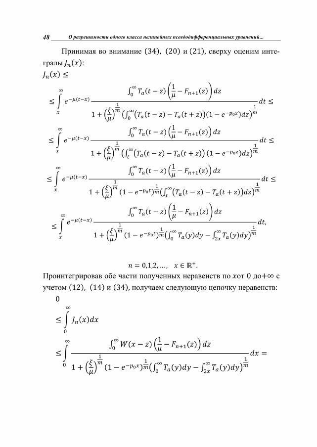
Принимая во внимание (34), (20) и(21), сверху оценим инте-гралы ( ): ( ) ≤
≤ ( ) ( − ) 1 − ( )1 + ( − ) − ( + ) (1 − ) ≤
≤ ( ) ( − ) 1 − ( )1 + ( − ) − ( + ) (1 − ) ≤
≤ ( ) ( − ) 1 − ( )1 + (1 − ) ( − ) − ( + ) ≤
≤ ( ) ( − ) 1 − ( )1 + (1 − ) ( ) − ( ) ,
= 0,1,2, … , ∈ ℝ . Проинтегрировав обе части полученных неравенств по от 0 до+∞ с учетом (12), (14) и (34), получаем следующую цепочку неравенств: 0≤ ( )
≤ ( − ) 1 − ( )1 + (1 − ) ( ) − ( ) =

Х.А. Хачатрян, Э.А. Андреасян 49
= ( − ) 1 − ( )1 + (1 − ) ( ) − ( ) +
+ ( − ) 1 − ( )1 + (1 − ) ( ) − ( ) ≤
≤ ( − ) 1 − ( ) + + 11 + ( − ) 1 − ( ) ,
где
≔ (1 − ) ( ) − ( ) =
= ( − 1) ( ) > 0, поскольку ( ) > 0, ∈ ℝ. Интегрируя обе части (35) по от 0 до +∞, с использованием выше полученной интегральной оценки для ( )и с учетом (12), (14), получаем следующую цепочку нера-венств: 0 ≤ 1 − ( )
≤ 1 ( ) + 1 ( ) + ( ) ≤

О разрешимости одного класса нелинейных псевдодифференциальных уравнений... 50
≤ 1 ( ) + 1 ( )+ ( − ) 1 − ( ) +
+ 11 + ( − ) 1 − ( ) , = 0,1,2, … . Изменением порядка интегрирования в последних двух интегралах правой части, полученных выше неравенств, будем иметь: 0 ≤ 1 − ( ) ≤ 1 ( ) + 1 ( ) +
+ 1 − ( ) ( − ) +
+ 11 + 1 − ( ) ( − ) ≤ ≤ 1 ( ) + 1 ( ) + 1 − ( ) ∙ ( ) + + 11 + 1 − ( ) ≤ 1 ( ) + 1 ( ) ++ ( ) , 11 + ∙ 1 − ( ) , = 0,1,2, ….
Так как > 0,0 < ( ) < 1, то
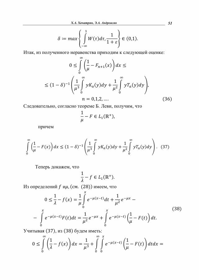
Х.А. Хачатрян, Э.А. Андреасян 51
≔ ( ) , 11 + ∈ (0,1). Итак, из полученного неравенства приходим к следующей оценке: 0 ≤ 1 − ( ) ≤
≤ (1 − ) 1 ( ) + 1 ( ) , = 0,1,2,….(36)
Следовательно, согласно теореме Б. Леви, получим, что 1 − ∈ (ℝ ), причем
1 − ( ) ≤ (1 − ) 1 ( ) + 1 ( ) .(37)
Теперь докажем, что 1 − ∈ (ℝ ). Из определений и , (см.(28))имеем, что 0 ≤ 1 − ( ) = 1 ( ) + 1 −− ( ) ( ) = 1 + ( ) 1 − ( ) .(38) Учитывая (37), из (38)будем иметь: 0 ≤ 1 − ( ) = 1 + ( ) 1 − ( ) =

О разрешимости одного класса нелинейных псевдодифференциальных уравнений... 52
= 1 + 1 − ( ) ( ) = 1 + 1 1 − ( ) ≤
≤ 1 + (1 − ) 1 ( ) + 1 ( ) . Следовательно, 1 − ∈ (ℝ ). Так как функция является нечетным продолжением на ℝ функции
, приходим к включениям (29). На основе вышеизложенных фактов, приходим к следующим результатам:
Теорема 1. Пусть функция обладает свойствами( ) − ( ), а > 0 −заданное число. Тогда граничная задача (1) − (2) имеет нетривиальное нечетное решение, причем ( ) ≥ 0, ∈ ℝ и ( ) < 0, ∈ ℝ .
Теоремa 2. Пусть функция удовлетворяет условиям ( ), ( ) и(30). Тогда для решения граничной задачи (1) − (2) при = 1 имеют место следующие включения: 1 ± ∈ ℝ∓ .
ЛИТЕРАТУРА
1. Владимиров В.С., Волович Я.И. О нелинейном уравнении динамики в теории -адической струны // ТМФ, (2004), 138:3. СС. 355−368. Theoret. аndMath. Phys. 138:3, (2004). СС. 297−309.
2. Volovich I. -adic string // Classical Quantum Gravity, (1987), 4:4, L83−L87.

Х.А. Хачатрян, Э.А. Андреасян 53
3. Хачатрян Х.А. О разрешимости некоторых классов нелинейных ин-тегральных уравнений в теории -адической струны // Изд-во «РАН». Сер. матем.,(2018), 82:2, 172−193.
4. Хачатрян Х.А. Разрешимость одного класса интегро-дифферен-циальных уравнений второго порядка с монотонной нелиней-ностью на полуоси // Изд-во «РАН». Сер. матем., (2010), 74:5. СС. 191−204.
5. Енгибарян Н.Б., Хачатрян А.Х. Интегро-дифференциальное уравне-ние нелокального взаимодействия волн // Матем. сб., (2007), 198:6. СС. 89−106.
6. Хачатрян Х.А. О нетривиальной разрешимости одного класса нели-нейных интегро-дифференциальных уравнений второго порядка // Матем. тр., (2012), 15:2. СС. 172-193.
7. Хачатрян Х.А., Петросян А.С. Об одной начально-краевой задаче для интегро-дифференциального уравнения второго порядка со сте-пенной нелинейностью // Изд-ов. вузов. Матем., (2018), 6. СС. 48−62.
8. Хачатрян Х.А. О разрешимости одной граничной задачи в -ади-ческой теории струн // Труды ММО, (2018), 79:1. СС. 1−16.
9. Колмогоров А.Н., Фомин В.С. Элементы теории функций и функ-ционального анализа. М.: ФИЗМАТЛИТ,7-е изд., (2004). 572 с.
10. Геворкян Г.Г., Енгибарян Н.Б. Новые теоремы для интегрального уравнения восстановления // Изд-во. НАН Армении. Матем., (1997), 32:1. СС. 5−20.
О разрешимости одного класса нелинейных псевдодифференциальных уравнений... 54
ON SOLVABILITY OF ONE CLASS OF NONLINEAR
PSEUDODIFFERENTIAL EQUATIONS ON THE WHOLE LINE
Kh. Khachatryan, E. Andreasyan
ABSTRACT
The work is devoted to the problem of solvability in the Sobolev (ℝ ) space of a class of pseudodifferential equations. Under certain conditions on the nonlinear part it is proved, that the considering equation has an odd solution ∈ (ℝ ), with a definite behavior at infinity and satisfies condition (0) = 0.
Keywords: nontrivial odd solution, Sobolev space, monotone, iterations, asymptoticsof the solution.
ԱՄԲՈՂՋ ԱՌԱՆՑՔԻ ՎՐԱ ՈՉ ԳԾԱՅԻՆ ՊՍԵՎԴՈԴԻՖԵՐԵՆՑԻԱԼ
ՀԱՎԱՍԱՐՈՒՄՆԵՐԻ ՄԵԿ ԴԱՍԻ ԼՈՒԾԵԼԻՈԻԹՅԱՆ ՄԱՍԻՆ
Խ.Ա. Խաչատրյան, Է.Ա..Անդրեասյան
ԱՄՓՈՓՈՒՄ
Աշխատանքը նվիրված է Սոբոլևի (ℝ ) տարածությունում պսևդո-
դիֆերենցիալ հավասարումների մեկդասի լուծելիությանը: Ոչ գծային մասի
վրա որոշակի պայմանների դեպքում ապացուցված է, որ դիտարկվող
հավասարումնունի ∈ (ℝ )կենտ լուծում՝ անվերջում որոշակի վարքով
և (0) = 0պայմանին բավարարող:
Հիմնաբառեր` ոչ տրիվիալկենտ լուծում, Սոբոլևի տարածություն,
մոնոտոնություն, մոտարկում, լուծմանասիմպտոտիկա:
Вестник РАУ № 2, 2018, 52-63 55
ФИЗИКА
УДК 669.017
ТЕМПЕРАТУРЫ КЮРИ
МАГНИТОУПОРЯДОЧЕННЫХ
СОЕДИНЕНИЙ В СИСТЕМЕ Gd5Si2-xGe2-xSn2x
Н.П. Арутюнян
Ереванский Государственный университет
АННОТАЦИЯ
Из температурных и полевых зависимостей намагниченности сплавов Gd5Si2-xGe2-xSn2x с 2x = 0,04; 0,05; 0,06; 0,08 были определе-ны температуры Кюри и максимальные изменения магнитной
части энтропии ΔS сплавов. Установлено, что при легировании
сплавов оловом значения температуры Кюри и ΔS сплавоввозрастают. Наблюдается значительное увеличение ΔS при уве-
личении почти на ΔTc≈18К< по сравнению с чистым Gd5Si2Ge2. Полученные данные свидетельствуют о том, что вышеуказанные

Температуры Кюри магнитоупорядоченных соединений в системе Gd5Si2-xGe2-xSn2x 56
соединения, обладая высоким магнитокалорическим эффектом, мо-гут быть использованы в магнитных рефрижераторах в качестве ра-бочего вещества.
Ключевые слова: полевые зависимости, намагниченность сплавов, температура Кюри.
1. Введение
В магнитоупорядоченных материалах (ферро- и антиферромаг-нетиках) при изменении внешнего магнитного поля в рабочем диапа-зоне температур возникает магнитокалорический эффект (МКЭ), обусловленный максимальным изменением магнитной части энтро-пии ΔSmax рабочего тела. Благодаря обнаружению значительных вели-чин калорических эффектов в области фазовых переходов типа поря-док-беcпорядок, методы охлаждения на основе МКЭ в настоящее вре-мя рассматриваются в качестве конкурентоспособных по отношению к традиционным методам охлаждения в широком интервале темпера-тур. Известно, что максимум величины ΔSM ферромагнетиков дости-гается в окрестности температуры фазового перехода ферромагне-тизм-парамагнетизм. Следовательно, точка Кюри материалов, из которых изготовлено рабочее тело магнитного холодильника, рабо-тающего, например, в области комнатных температур, должна лежать вблизи ≈ 293К. Такими свойствами обладают сплавы тяжелых ред-коземельных металлов на основе гадолиния [1–3].
В работе [4] показано, что эффективным магнитокалорическим материалом, по сравнению с гадолинием, является соединение Gd5Si2Ge2 с гигантским МКЭ при = 262К. Однако вышеуказанное соединение в качестве хладагента в области температур T≥ 262К не-достаточно эффективно, так как максимум температурной зависи-мостиΔS должен находиться в интервале температур выше точки Кюри данного образца.

Н.П. Арутюнян 57
В работах [5, 6] авторами были измерены намагниченность и магнитную восприимчивость магнитоупорядоченных соединений в системеGd5SixGe4–xс частичным замещением атомов кремния и герма-ния изовалентными атомами олова (Sn). Было показано, что частичное замещение кремния и германия оловом приводит к возрастанию тем-пературы Кюри и увеличению магнитной части энтропииΔS .
В настоящей работе представлены результаты исследований маг-нитоупорядоченных соединений системы Gd5Si2–xGe2–xSn2xс новым стехиометрическим составом (2x= 0, 04; 0,05; 0,06; 0,08). Для опреде-ления скачка энтропии ΔSM был использован метод расчета намагни-ченности данного образца на основе известных полевых и температур-ных зависимостей. Изотермическое изменение энтропии в исследуе-мом интервале магнитного поля вычислялось по формуле: ∆ = (1), полученном из уравнений Максвелла [7]. = H(2)
Так как намагниченность измеряется при дискретных значениях магнитного поля, то, согласно [8], выражение (1) может быть аппрок-симировано формулой: ∆ = ∑ ( − )∆ ,(3)
где Miи Mi+1– намагниченности, измеренные в полях H при темпера-турах TiиTi+1, соответственно.
2. Методикаэксперимента и обсуждение результатов.
Поликристаллические образцы соединений Gd5Si2–xGe2–xSn2xс 2x= 0; 0,03; 0,04; 0,06; 0,08 были синтезированы в гелиевой атмосфере индукционным методом и идентифицированы рентгенографически на дифрактометре ДРОН-2 по методике, описанной в [5]. Намагничен-ность образцов измерялась методом Фонера [9] путем регистрации
Температуры Кюри магнитоупорядоченных соединений в системе Gd5Si2-xGe2-xSn2x 58
э.д.с. разбаланса, возникающей в системе из двух измерительных ка-тушек, включенных навстречу друг другу при вибрировании образца в магнитном поле. Вибратором служил акустический динамик, подк-люченный к генератору низкочастотных колебаний. Измерения намаг-ниченности образцов проводились в постоянном магнитном поле, ко-торое менялось в пределах 0–1, 0 Т. Температура образцов менялась в интервале 250–300К.
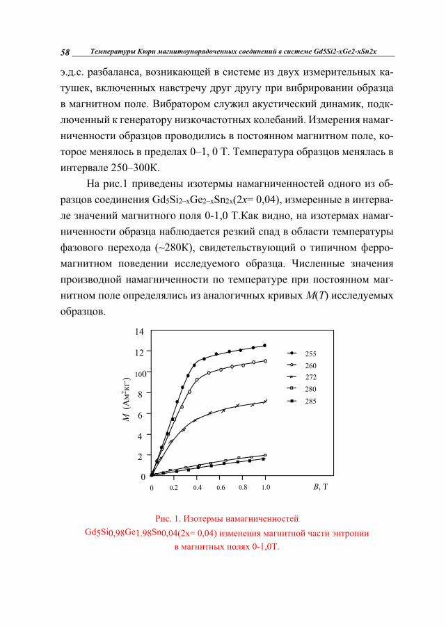
На рис.1 приведены изотермы намагниченностей одного из об-разцов соединения Gd5Si2–xGe2–xSn2x(2x= 0,04), измеренные в интерва-ле значений магнитного поля 0-1,0 Т.Как видно, на изотермах намаг-ниченности образца наблюдается резкий спад в области температуры фазового перехода (~280К), свидетельствующий о типичном ферро-магнитном поведении исследуемого образца. Численные значения производной намагниченности по температуре при постоянном маг-нитном поле определялись из аналогичных кривых M(T) исследуемых образцов.
Рис. 1. Изотермы намагниченностей
Gd5Si0,98Ge1.98Sn0,04(2x= 0,04) изменения магнитной части энтропии в магнитных полях 0-1,0Т.
M (Ам2 к
г- )
2
4
6
100
8
12
0 0.2 0.8 1.0 0.4 0.6
14
0
285
255 260 272 280
В, Т
Н.П. Арутюнян 59
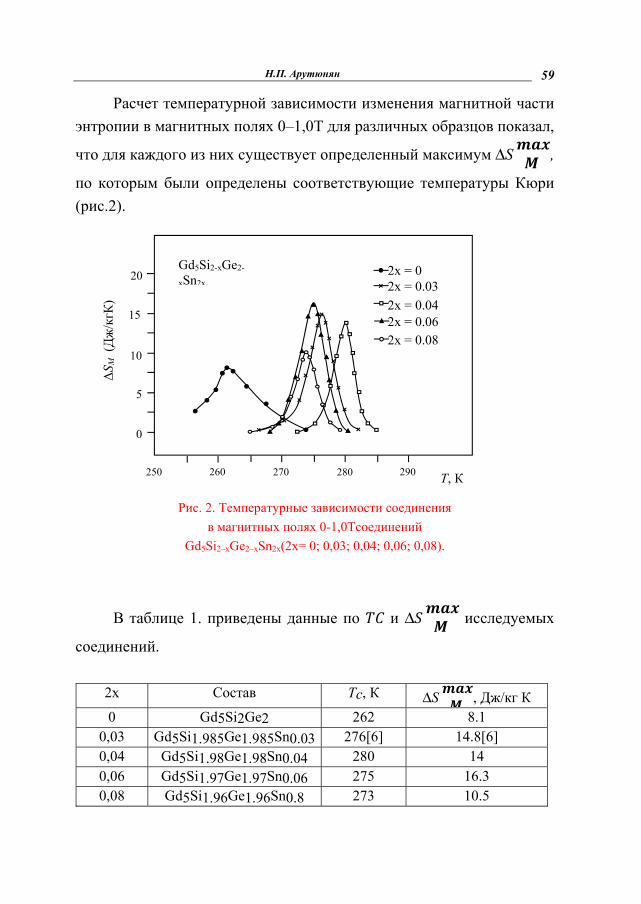
Расчет температурной зависимости изменения магнитной части энтропии в магнитных полях 0–1,0Т для различных образцов показал,
что для каждого из них существует определенный максимум ΔS ,
по которым были определены соответствующие температуры Кюри (рис.2).
Рис. 2. Температурные зависимости соединения в магнитных полях 0-1,0Тсоединений
Gd5Si2–xGe2–xSn2x(2x= 0; 0,03; 0,04; 0,06; 0,08).
В таблице 1. приведены данные по и ΔS исследуемых
соединений. 2x Состав Tc, К ΔS , Дж/кг К 0 Gd5Si2Ge2 262 8.1
0,03 Gd5Si1.985Ge1.985Sn0.03 276[6] 14.8[6] 0,04 Gd5Si1.98Ge1.98Sn0.04 280 14 0,06 Gd5Si1.97Ge1.97Sn0.06 275 16.3 0,08 Gd5Si1.96Ge1.96Sn0.8 273 10.5
Т, К
ΔSM
(Дж
/кгК
)
0
5
10
15
20
250 260 270 280 290
Gd5Si2-xGe2-
xSn2x
2x = 0.08
2x = 0 2x = 0.03 2x = 0.04 2x = 0.06

Температуры Кюри магнитоупорядоченных соединений в системе Gd5Si2-xGe2-xSn2x 60
Как видно из таблицы, частичное замещение кремния и германия оловом приводит квозрастаниюTc по сравнению с чистым Gd5Si2Ge2 наΔTc ≈18К (2x=0,04), что на четыре градуса превышает результат, полученный в работе [6]. Как было сказано в работе [6], значительный-
рост ΔS для легированных сплавов, по сравнению с чистыми
Gd5Si2Ge2 можно объяснить уменьшением длины свободного пробе-га электронов, связанным с увеличением эффективного сечения
рассеяния электронов на ионах Sn4+, имеющих больший ионный ра-
диус, чем Si4+ и Ge4+. Это обстоятельство приводит к усилению s–f обменного взаимодействия между магнитоактивными ионами гадоли-ния, подобно изложенному в [10].
3. Заключение Известно, что магнито-калорический эффект в магнитоупорядо-
ченных соединениях возникает при изменении внешнего магнитного поля в рабочем диапазоне температур и он обусловен максимальным изменением магнитной части энтропии ΔS образца. Поскольку мак-симум величины ΔS ферромагнетиков достигается в окрестности температуры фазового перехода ферромагнетизм-паромагнетизм, то температура Кюри может играть важнейшую роль в поисаках мате-риалов, из которых изготовлено рабочее тело магнитных холодильни-ков. Для определения температуры Кюри в работе были измерены намагниченности сплавов Gd5Si2–xGe2–xSn2xс 2x=0,04; 0,05; 0,06; 0,08, и из их температурных и полевых зависимостей определены температу-ры Кюри и максимальные изменения магнитной части энтропии ΔS . Установлено, что при легировании сплавов оловом значения температуры Кюри иΔS сплавов возрастают. Наблюдается значи-
тельное увеличение температуры Кюри почти на ΔT≈18К, по сравне-нию с чистым Gd5Si2Ge2.
Н.П. Арутюнян 61
Полученные данные свидетельствуют о том, что вышеуказанные соединения, обладая высоким магнито-калорическим эффектом, мо-гут быть использованы в магнитных рефрижераторах, работающих в области комнатных температур вблизи ≈ 293К в качестве рабочего вещества.
ЛИТЕРАТУРА
1. Brown G.V., Appl J. Phys.,47,3673 (1976). 2. Tishin A.M. Gryogenics, 30,720 (1990). 3. Никитин С.А. Магнитные свойства редкоземельных металлов и их
сплавов. М. Изд-во. МГУ, 1989. 4. Pecharsky V.K., Gschneidner K.A. Phys. Rev. Lett., 78, (№ 23), 4494
(1997). 5. Агабабян Э.В., Арутюнян Н.П. Извд-во. НАН Армении, Физика,
44, 294 (2009). 6. Агабабян Э.В., Арутюнян Н.П. Изд-во. НАН Армении, Физика, 50,
264 (2015). 7. Bohigas X., del Barco E., Sales M., Tejada J., Magn J. Mater. 196–197,
455 (1999). 8. McMichael R.D., Rittel J.J., Shull R.D., Appl J. Phys., 73, 6946(1993). 9. Чечерников В.И. Магнитные измерения. М. Изд-во. МГУ, 1963. 10. Адамян В.Е., Шароян Э.Г. Изд-во. НАН Армении, Физика, 36, 94
(2001).
Температуры Кюри магнитоупорядоченных соединений в системе Gd5Si2-xGe2-xSn2x 62
MAGNETICALLY ORDERED COMPOUNDS IN THE
GD5SI2–XGE2–XSN2X SYSTEM AT CURIE’S TEMPERATURES
N. Harutyunyan
ABSTRACT
Maximal changes of the magnetic part of entropy ΔS of alloys versus
temperature and field dependences of Gd5Si2–xGe2–xSn2x alloys with 2x=0,03-0,08 are determined. It is established as a result of Sn doping leads to increasing the
values Tc (in the case of, 2x=0,04) and ΔS in alloys. The obtained data allow
to conclude that the above mentioned magnetically ordered compounds can be occupied in magnetocaloric effect and can be used as a working substance of magnetic refrigerators.
Keywords: полевые зависимости, намагниченность сплавов, темпера-тура Кюри.
Gd5Si2–xGe2–xSn2x ՀԱՄԱԿԱՐԳԻ ՄԱԳՆԻՍԱԿԱՐԳԱՎՈՐՎԱԾ
ՄԻԱՑՈՒԹՅՈՒՆՆԵՐԻ ԿՅՈՒՐԻԻ ՋԵՐՄԱՍՏԻՃԱՆՆԵՐԸ
Ն.Պ. Հարությունյան
ԱՄՓՈՓՈՒՄ
2x=0,03-0,08 արժեքներով Gd5Si2–xGe2–xSn2x համաձուլվածքների
մագնիսականության ջերմաստիճանային և դաշտային կախվածություն-
ներից որոշված են համաձուլվածքների Tc Կյուրիի ջերմաստիճանները և
էնթրոպիայի մագնիսական բաժնի ΔS -ի առավելագույն արժեքները:
Հայտնաբերված է, որ անագով լեգիրման հետևանքով աճում է ինչպես

Н.П. Арутюнян 63
համաձուլվածքների Կյուրիի ջերմաստիճանները (ΔT≈ 18Կ, 2x=0,04 դեպ-
քում), այնպես էլ ΔS -ի արժեքները: Ստացված արդյունքները վկայում
են այնմասին, որ վերը նշված մագնիսակարգավորված միացությունները
կարող են տիրապետել բարձր մագնիսակալորիական երևույթով և կարող
են կիրառվել իբրև բանող նյութեր մագնիսական սառնարաններում:
Հիմնաբառեր`полевые зависимости, намагниченность сплавов, темпера-тура Кюри.
Вестник РАУ № 2, 2018, 64-7664
УДК 621.376
ИЗВЛЕЧЕНИЕ И РАСЧЕТ КЛЮЧЕВЫХ
ХАРАКТЕРИСТИК СИГНАЛА ДЛЯ
КЛАССИФИКАЦИИ АНАЛОГОВЫХ МОДУЛЯЦИЙ
А.М. Тантушян
Институт радиофизики и электроники (НАН РА)
АННОТАЦИЯ
Автоматическое распознавание модуляций является одним из важнейших задач систем связи. Для распознавания типа модуляции, без предварительных данных о сигнале, необходимо в этапе предва-рительной обработки сигнала извлечь ключевые характеристики. В данной научной статье описаны ключевые характеристики сигналов, которые применяются для автоматического распознавания аналого-вых модуляций, ипредставлен их расчет в среде графического про-граммирования Lab VIEW.
Ключевые слова: автоматическое распознавание модуляций, ключевые характеристики сигнала, аналоговые модуляции.
Введение
Системы aвтоматического распознавания модуляций (АРМ) состоят из трех блоков: предварительной обработки сигнала, класси-

А.М. Тантушян 65
фикатора и демодулятора. В блоке предобработки принятый «неиз-вестный» сигнал разделяется на сегменты равной длины, из которых и извлекаются ключевые характеристики. Ключевые характеристики сигнала – это те данные, которые описывают конкретные особенности данного сигнала. При правильно выбранной группе ключевых харак-теристик можно с большой точностью определить тип модуляции сиг-нала, поскольку значения этих характеристик для каждого типа моду-лированного сигнала будут уникальными. Существуют типы модуля-ций, для которых значения какой-то характеристики будут близкими или одинаковыми, но не существуют такие типы модуляций, для кото-рых значения всех характеристик одинаковы. Для расчета ключевых характеристик использовались такие параметры как: мгновенная амп-литуда и фаза, и спектр мощности сигнала. В случае, когда данные о сигнале неизвестны, возникают проблемы, связанные с расчетом мгновенной частоты, амплитуды и фазы, которые подробно описаны в “Appendix A” работы Аззоуза и Нанди [1]. Так как в данной работе рассмотрены моделированные сигналы, то, соответственно, считается, что частота несущей известна.
В данной работе рассмотрены DSB (double side band), SSB (single side band) и FM (frequency modulation) типы аналоговых модуляций и ключевые характеристики [1], предназначенные для их распознавания. Представлено подробное описание извлечения и расчета этих характе-ристик в среде графического программирования Lab VIEW и резуль-таты тестов автоматического распознавания с помощью искусствен-ной нейронной сети.
Целью работы является описание практической реализации и ре-шения задачи автоматического распознавания аналоговых модуляций, для чего в среде графического программирования Lab VIEW, на осно-ве исследованной литературы, был разработан алгоритм для извлече-ния ключевых характеристик моделированных аналоговых модулиро-ванных сигналов. Полученные данные были поданы на входы ранее
Извлечение и расчет ключевых характеристик сигнала... 66
разработанной базовой модели искусственной нейронной сети [2], ко-торая использовалась в качестве классификатора для автоматического распознавания.
1. DSB модуляция. При DSB амплитудной модуляции модули-рованный сигнал ( )описывается следующимиизвестным соотноше-нием [3]: ( ) = ( ) (1 + ( )) ( )(1), где ( ) – амплитуда несущей, – индекс модуляции, ( ) – это ннформационный сигнал, а – несущая частота. Когда модулирую-щая функция ( )периодична и выражается рядом Фурье, тогда имеем: ( ) = cos( − )(2), где k = 1, 2, … , N, и соответственно амплитуда и начальная фаза k – го колебания, а – часота сигнала.Из (1) и (2) следует: ( ) = ( ) 1 + cos( − ) ( ) =
= ( ) ( ) + 2 cos[( + ) − ] +
+ ∑ cos[( − ) + ] (3). Таким образом, спектр DSB модулированного сигнала состоит
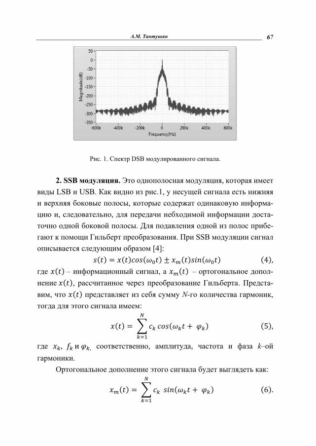
из колебания несущей частоты , колебаний с суммарными частота-ми( + )и разностными частотами ( − ). В частотном представлении – это две боковые полосы, с левой и правой стороны несущей, которые называются LSB (lower side band) нижняя боковая полоса и USB (upper side band) верхняя боковая полоса. На рис.1 отоб-ражен спектр DSB модулированного сигнала, где нижняя боковая по-лоса симметрична верхней боковой полосе относительно несущей частоты.
А.М. Тантушян 67
Рис. 1. Спектр DSB модулированного сигнала.
2. SSB модуляция. Это однополосная модуляция, которая имеет виды LSB и USB. Как видно из рис.1, у несущей сигнала есть нижняя и верхняя боковые полосы, которые содержат одинаковую информа-цию и, следовательно, для передачи небходимой информации доста-точно одной боковой полосы. Для подавления одной из полос прибе-гают к помощи Гильберт преобразования. При SSB модуляции сигнал описывается следующим образом [4]: ( ) = ( ) ( ) ± ( ) ( )(4), где ( )– информационный сигнал, а ( )– ортогональное допол-нение ( ), рассчитанное через преобразование Гильберта. Предста-вим, что ( ) представляет из себя сумму N-го количества гармоник, тогда для этого сигнала имеем: ( ) = ( + )(5), где , и , соответственно, амплитуда, частота и фаза k–ой гармоники.
Ортогональное дополнение этого сигнала будет выглядеть как: ( ) = ( + )(6).

Извлечение и расчет ключевых характеристик сигнала... 68
Итак, подставив уравнения (5) и (6) в (4) для SSB модуляции, полу-чим ( ) сигнал в следующем представлении: ( ) = ( ± ) + (7).
На рис. 2 изображены спектры LSB (а) и USB (б) модулирован-ных сигналов.
а) LSB
б) USB
Рис. 2. Спектры LSB (а) и USB (б) модулированных сигналов.
3. FM модуляция. В случае модуляции сигналов с постоянной амплитудой, т.е. в случае частотной и фазовой модуляции, колебание можно представить в следующей форме [3]:
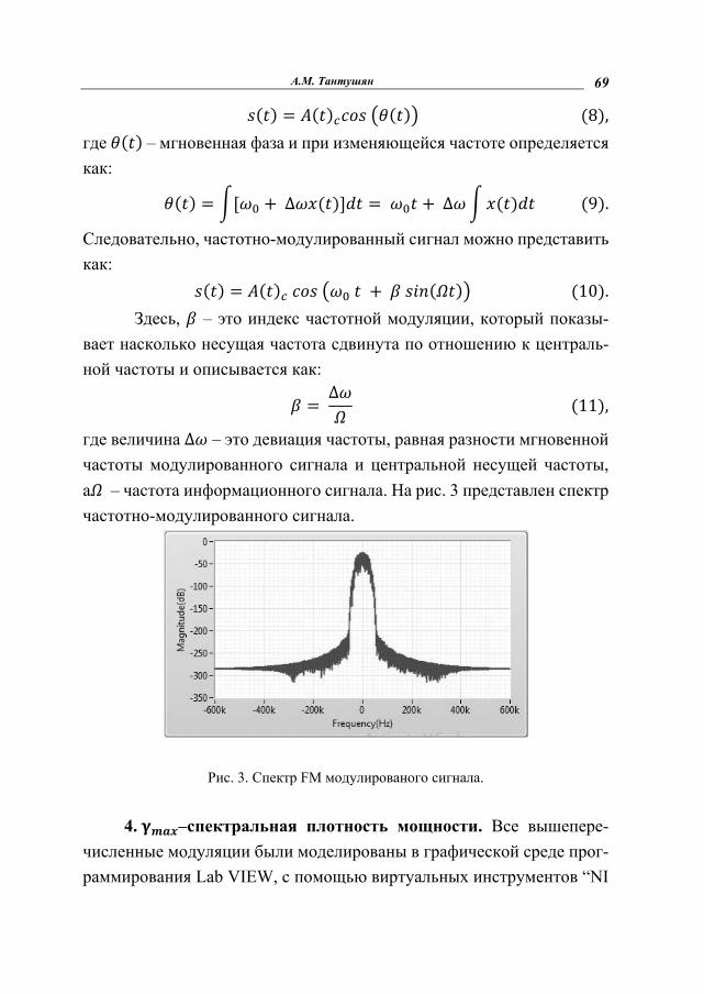
А.М. Тантушян 69( ) = ( ) ( ) (8), где ( ) – мгновенная фаза и при изменяющейся частоте определяется как: ( ) = [ +∆ ( )] = +∆ ( ) (9). Следовательно, частотно-модулированный сигнал можно представить как: ( ) = ( ) + ( ) (10).
Здесь, – это индекс частотной модуляции, который показы-вает насколько несущая частота сдвинута по отношению к централь-ной частоты и описывается как: =∆ (11), где величина ∆ – это девиация частоты, равная разности мгновенной частоты модулированного сигнала и центральной несущей частоты, а – частота информационного сигнала. На рис. 3 представлен спектр частотно-модулированного сигнала.
Рис. 3. Спектр FM модулированого сигнала.
4. –спектральная плотность мощности. Все вышепере-численные модуляции были моделированы в графической среде прог-раммирования Lab VIEW, с помощью виртуальных инструментов “NI
Извлечение и расчет ключевых характеристик сигнала... 70
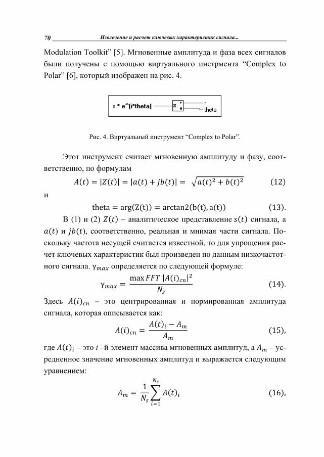
Modulation Toolkit” [5]. Мгновенные амплитуда и фаза всех сигналов были получены с помощью виртуального инстрмента “Complex to Polar” [6], который изображен на рис. 4.
Рис. 4. Виртуальный инструмент “Complex to Polar”.
Этот инструмент считает мгновенную амплитуду и фазу, соот-ветственно, по формулам ( ) = | ( )| = | ( ) + ( )| = ( ) + ( ) (12) и theta = arg(Z(t)) = arctan2(b(t), a(t))(13).
В (1) и (2) ( ) – аналитическое представление ( ) сигнала, а ( ) и ( ), соответственно, реальная и мнимая части сигнала. По-скольку частота несущей считается известной, то для упрощения рас-чет ключевых характеристик был произведен по данным низкочастот-ного сигнала. γ определяется по следующей формуле: γ = max | ( ) | (14). Здесь ( ) – это центрированная и нормированная амплитуда сигнала, которая описывается как: ( ) = ( ) − (15), где ( ) – это i –й элемент массива мгновенных амплитуд, а – ус-редненное значение мгновенных амплитуд и выражается следующим уравнением: = 1 ( ) (16),

А.М. Тантушян 71
где – количество точек взятого сегмента сигнала. Как видно из фор-мулы (14), для расчета γ находим максимальное значение спектра мощности и делим на общее количество точек.
Итак, получаем, что γ – это максимальная спектральная плот-ность мощности. Это ключевая характеристика применяется для авто-матического распознавании FM аналоговой модуляции и DSB, SSB как другую группу. Поскольку амплитуда FM модулированных сигна-лов – постоянная величина, то следует, что такие сигналы не имеют амплитудную информацию и их центрированная и нормированная амплитуда равна нулю. Следовательно, значение γ для частотно-модулированных сигналов всегда стремится к нулю, а для DSB, SSB модуляций имеет значение больше нуля. На рис. 5 изображена часть кода, выполняющая расчет γ - а.
Рис. 5. Расчет – а в Lab VIEW.
5. – стандартная девиация абсолютного значения центри-
рованной нелинейной компоненты мгновенной фазы. Эта ключе-вая характеристика определяется по следующей формуле:
σ = 1 ( )( ) − 1 | ( ) |( ) (17), где ( ) – центрированная нелинейная компонента мгновенной фа-зы, C – количество точек для которых ( ) > , где ( ) – нормиро-

Извлечение и расчет ключевых характеристик сигнала... 72
ванная мгновенная амплитуда,а – это пороговое значение амплиту-ды, ниже которой расчет не целесообразен из-за уровня шумов. В уравнении (17) ( ) выражается следующим уравнением: ( ) = ( ) (18),
Данная ключевая характеристика применяется для распознава-ния аналоговых модуляций, имеющих абсолютную фазовую информа-цию и тех, которые не имеют. Рассмотрим мгновенные значения фазы для DSB модуляции. Представим сигнал ( ) в аналитическом виде как: ( ) = ( ) (19).
Из уравнения (19) следует, что мгновенная фаза при DSB моду-ляции примет два значения: ( ) = 2 , ( ) > 02 + , ( ) < 0(20).
Поскольку главным внедрителем линейной компоненты фазы является несущая, то после удаления линейной компоненты 2 получаем, что фаза получает значения 0 и . Для центрирования фазы небходимо от обеих значений отнять , из чего следует, что после уда-
ления линейной компоненты и центрированияполучаем, что значение абсолютной фазы - это постоянная величина и равна | |. Это означает,
что, в отличие от остальных типов, DSB модулировнный сигнал не имеет абсолютной фазовой информации. Следовательно этот вывод позволяет применить данную ключевую характеритику для различе-ния DSB модуляции и других видов модуляций.
Итак, поскольку расчет был проведен по данным низкочастотно-го сигнала, считается, что нелинейная компонента фаза и есть фаза низкочастотного сигнала. На рис. 6 изображена часть кода, выполняю-щая расчет σ .

А.М. Тантушян 73
Рис.6. Расчет σаф в LabVIEW.
6. P – спектральная симметричность. Ключевая характеристи-ка сигнала P описывает симметричность спектра в смысле левой и пра-вой боковых полос несущей. Она применяется для отличения SSB (LSB, USB) модуляции и DSB, FM модуляций, поскольку, как уже от-мечалось, при SSB модуляции левая или правая боковая полоса фильт-руется, что нарушает симметричность спектра. В то же время спектр DSB и FM модулированных сигналов симметричен. Симметричность спектра определяется следующим уравнением: = −+ (21). В уравнении (21) и , соответственно, спектральная мощность ниж-ней и верхней боковых полос и определяются соответственно как: = | ( )| (22),
= | ( + + 1)| (23). Здесь – Фурье преобразование сигнала, а + 1 – это номер точки соответстующей несущей. определяется как: = − 1(24). Итак, для расчета и берется количество точек и значение мощ-ности несущей из расчетов исключается. Как видно из уравнения (21)
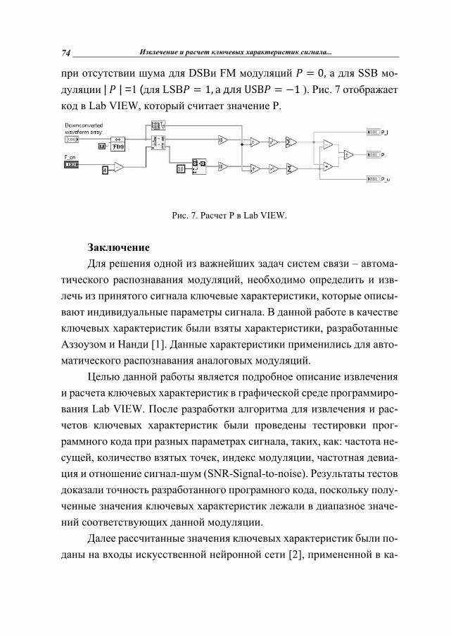
Извлечение и расчет ключевых характеристик сигнала... 74
при отсутствии шума для DSBи FM модуляций = 0, а для SSB мо-дуляции | | =1 (для LSB = 1, адляUSB = −1 ). Рис. 7 отображает код в Lab VIEW, который считает значение P.
Рис. 7. Расчет P в Lab VIEW.
Заключение
Для решения одной из важнейших задач систем связи – автома-тического распознавания модуляций, необходимо определить и изв-лечь из принятого сигнала ключевые характеристики, которые описы-вают индивидуальные параметры сигнала. В данной работе в качестве ключевых характеристик были взяты характеристики, разработанные Аззоузом и Нанди [1]. Данные характеристики применились для авто-матического распознавания аналоговых модуляций.
Целью данной работы является подробное описание извлечения и расчета ключевых характеристик в графической среде программиро-вания Lab VIEW. После разработки алгоритма для извлечения и рас-четов ключевых характеристик были проведены тестировки прог-раммного кода при разных параметрах сигнала, таких, как: частота не-сущей, количество взятых точек, индекс модуляции, частотная девиа-ция и отношение сигнал-шум (SNR-Signal-to-noise). Результаты тестов доказали точность разработанного програмного кода, поскольку полу-ченные значения ключевых характеристик лежали в диапазное значе-ний соответствующих данной модуляции.
Далее рассчитанные значения ключевых характеристик были по-даны на входы искусственной нейронной сети [2], примененной в ка-

А.М. Тантушян 75
честве классификатора для распознавания вида модуляций. Для про-верки точности классификации для каждого типа модуляции были реа-лизованы 100 симуляций. Результаты тестов распознавания вида мо-дуляции с помощью искусственой нейронной сети при разных значе-ниях SNR, отображены в таблице 1.
Таблица 1.
Результаты распознавания видов модуляций
SNR DSB LSB USB FM Inf. 100% 100% 100% 100% 20dB 100% 100% 100% 100% 15dB 100% 100% 99% 100% 10dB 96% 100% 92% 100% 5dB 82% 100% 82% 100%
ЛИТЕРАТУРА
1. Azzouz E., Nandi A. Automatic Modulation Recognition of Communi-cation Signals. Kluwer Academic Publishers, Dordrecht, (1996), 214 p.
2. Гулян А.Г., Севоян О.Ж., Тантушян А.М. Автоматическое распозна-вание четырех видов симулированных сигналов с помощью ис-кусственной нейронной сети. Известия. Т. 4. СС. 467–471. (2017).
3. Харкевич А.А. Основы радиотехники, Государственное издательст-во литературы по вопросам связи и радио. М. (1962).
4. http://www.dsplib.ru/content/ssb/ssb.html 5. http://sine.ni.com/nips/cds/view/p/lang/ru/nid/210568 6. http://zone.ni.com/reference/en-XX/help/371361P-
01/glang/complex_to_polar/

Извлечение и расчет ключевых характеристик сигнала... 76
SIGNAL’S KEY FEATURES EXTRACTION AND CALCULATION FOR
ANALOG MODULATION CLASSIFICATION
A.Tantushyan
ABSTRACT
Automatic modulation recognition is one of the most important tasks for telecommunication systems. For modulation type recognition, without any prior information about signal, it is necessary to extract key features during the phase of signal preprocessing. The key features for analog modulation recognition are described in this paper. Their calculations in the LabVIEW graphical programming environment are presented.
Keywords: automatic modulation recognition, key features of signal, analog modulations.
ԱԶԴԱՆՇԱՆԻ ՀԻՄՆԱԿԱՆ ԲՆՈՒԹԱԳՐԵՐԻ ԱՌԱՆՁՆԱՑՈՒՄՆ
ՈՒ ՀԱՇՎԱՐԿԸ ԱՆԱԼՈԳԱՅԻՆ ՄՈԴՈՒԼՅԱՑԻԱՆԵՐԻ
ԴԱՍԱԿԱՐԳՄԱՆ ՀԱՄԱՐ
Ա.Մ․Թանթուշյան
ԱՄՓՈՓՈՒՄ
Մոդուլացումների ավտոմատացված ճանաչումը հեռահորդակցու-
թյան համակարգերի ամենակարևորագույն խնդիրներից մեկն է։ Մոդու-
լացումների ավտոմատացված ճանաչման համար՝ առանց որևէ սկզբնական
ինֆորմացիայի ազդանշանի մասին, հարկավոր է ազդանշանի նախա-
մշակման փուլում առանձնացնել հիմնական բնութագրերը։ Այս աշխատան-
քի մեջ նկարագրված են անալոգային մոդուլացումների ավտոմատացված
ճանաչման դեպքում կիրառվող հիմնական բնութագրերը։ Ներկայացված է
դրանց հաշվարկը LabVIEW գրաֆիկական ծրագրավորման միջավայրում։
Հիմնաբառեր՝ մոդուլացումների ավտոմատացված ճանաչում, ազդա-
նշանի հիմնական բնութագրեր, անալոգային մոդուլացումներ։

Вестник РАУ № 2, 2018, 77-85 77
БИОЛОГИЯ
UDC.599.323.41.591.111
THE ECOLGY OF URAL FIELD MICE APODEMUS
URALENSIS PALLAS, 1811 PREVAILING IN ARTSAKH
FAUNA AND THEIR BIOOD INDEXES DEPENDING ON
THE VERTICAL ZONING
V. Hayrapetyan
Ministry of Nature Protection and Natural Resource RA,
«“Green Artsakh” Biosfere omplex»
ABSTRACT
In this work, the issues concerning the prevalence, ecology and biology of Ural field mice are discussed. Not only their types of activities are clarified, but also the dynamics of the number and the reasons for the change in number. Special attention is paid to the changes of the blood index of these beasts depending on the season and vertical zoning.
Keywords: Artsakh, Ural field mouse, ecology, blood.

The ecolgy of ural field mice apodemus uralensis pallas, 1811 prevailing in artsakh fauna... 78
Introduction: As everywhere in the Artsakh Republic also the order Rodentia takes the 1st place with its variety of types, the area of prevalence, flexibility of ecology and number.
Ural field mice are also the components of nourishment for predators which are hunted. They are also the bearers and transmitters of some pathogens which can cause diseases of people and animals, and the main pests for crops in agriculture. This way the clarification of the issues concerning the ecology, biology and blood indexes of Ural field mice Apodemus uralensis Pallas, 1811 is of great importance.
Material and methods: The main material for this work are our surveys and accumulated material from 1999 to 2017. The material was collected from the plains, as well as foothills and medium mountainous regions of Artsakh. To study the ecological peculiarities we used the classical methods accepted in biology [3, 5, 6, 7, 10].To study the blood indexes we used the methods accepted in physiology [8]. The hunting was carried out by bow-shaped and live traps, as baits pieces of bread dunked in oil, sausages and other things were used. The height of the dwellings of these beasts was measured with Magellan GPS-315.
The summary of results: In our conditions, Ural field mice are common everywhere, and in some places even prevalent. Their dwellings are now situated in various places – in different forests, bushes, cultivated lands near forests and people’s houses. Nevertheless, they are very few in subalpine zones and are found only in the forests near subalpine zone, bushes, meadows near it, river valleys. Their dwellings are created in hiding places of any type, sometimes they dig their nests. For reproduction purposes, they carefully “furnish” their nests, which can be two-ply or spherical.
Though these beasts have a wide area of prevalence and are densely populated, a sharp fluctuation is recorded in their number in different years.
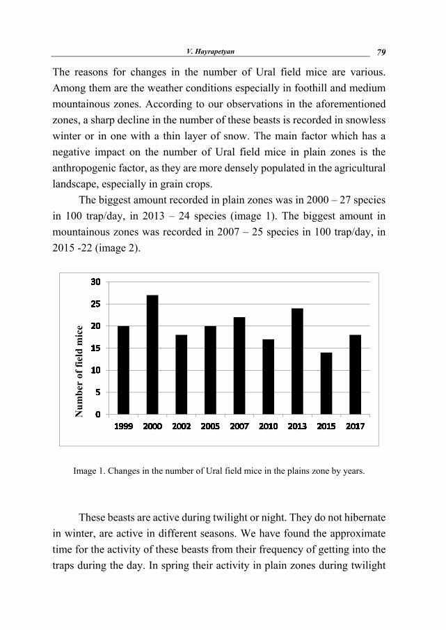
V. Hayrapetyan 79
The reasons for changes in the number of Ural field mice are various. Among them are the weather conditions especially in foothill and medium mountainous zones. According to our observations in the aforementioned zones, a sharp decline in the number of these beasts is recorded in snowless winter or in one with a thin layer of snow. The main factor which has a negative impact on the number of Ural field mice in plain zones is the anthropogenic factor, as they are more densely populated in the agricultural landscape, especially in grain crops.
The biggest amount recorded in plain zones was in 2000 – 27 species in 100 trap/day, in 2013 – 24 species (image 1). The biggest amount in mountainous zones was recorded in 2007 – 25 species in 100 trap/day, in 2015 -22 (image 2).
Image 1. Changes in the number of Ural field mice in the plains zone by years.
These beasts are active during twilight or night. They do not hibernate
in winter, are active in different seasons. We have found the approximate time for the activity of these beasts from their frequency of getting into the traps during the day. In spring their activity in plain zones during twilight
Nu
mb
er o
f fi
eld
mic
e

The ecolgy of ural field mice apodemus uralensis pallas, 1811 prevailing in artsakh fauna... 80
lasts from 20:00 to 23:00. At midnight their activity is slowed down and rare species are trapped, a big amount of which being males, barren females and young ones. The second rise of activity lasts mainly from 03:00 to 08:00. In the daytime activity also slows down. Their activity in the forest, foothills and mountainous areas is recorded immediately after the sunset and before the sunrise. They do not have a clearly emphasised activity in spring and summer. Their activity slows down in the morning and at night and instead, they become more active during the day. In rainy weather, they also move slowly but keep their mobility in the hiding places [2, 9].
Image 2. Changes in the number of Ural field mice in the mountainous zone by years.
In our conditions, especially in plain zones, they breed from 4 to 5 times, in middel and high mountainous zones from 2 to 3 times. The pregnancy lasts 28-29 days and they have 6-8 cubs. They become mature in 85-95 days [1,4,5]. During the observations, we have found one not emphasised case of moulting in spring, moulting in autumn is not excluded as well.
Num
ber o
f fie
ld m
cie

V. Hayrapetyan 81
The evaluation of the blood system can be described as the reaction of the organism to the changing conditions of the environment.
The indexes of Ural field mice blood were studied in plain as well as in mountainous zones during different seasons.
The indexes of Ural field mice (♂ and ♀) blood in plain zones (500 m a.s.l.) are presented in the table 1.
Table 1
The studied blood indexes of Ural field mice in the plain zones
As it can be seen from Table 1, the concentration of hemoglobin on the lowest level in males and females is recorded in the summer, relatively high in spring and fall, and the highest in winter. The red blood cell count of both males and females is also high in winter. The amount of eosinophil is unchanged in any season. The amount of leukocytes of females is the highest in summer.
Studied feature Sex Winter Spring Summer Autumn
Hemoglobin g/l ♂ 168 160 150 155 ♀ 159 156 141 143
Erythrocytes (million) ♂ 9,5 8,7 7,9 6,8 ♀ 9,1 8,5 7,3 6,2
leucocytes (thousand) ♂ 5,2 5,8 5,5 5,2 ♀ 5,1 5,7 6,1 5,4
Segmented neutrophil % ♂ 41,7 47,8 46,3 43,6 ♀ 44,3 49,3 45,7 40,6
Eosinophil % ♂ 1 1,02 1 1 ♀ 1,1 1 1 1
Monocyte % ♂ 4,21 4,87 4,45 3,87 ♀ 3,95 4,65 4,91 4,12
Lymphocyte % ♂ 47,75 46,32 48.47 51,42 ♀ 47,24 41,82 47,87 50,42
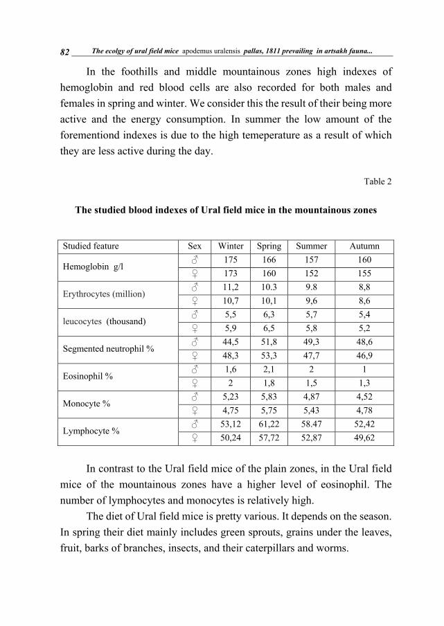
The ecolgy of ural field mice apodemus uralensis pallas, 1811 prevailing in artsakh fauna... 82
In the foothills and middle mountainous zones high indexes of hemoglobin and red blood cells are also recorded for both males and females in spring and winter. We consider this the result of their being more active and the energy consumption. In summer the low amount of the forementiond indexes is due to the high temeperature as a result of which they are less active during the day.
Table 2
The studied blood indexes of Ural field mice in the mountainous zones
In contrast to the Ural field mice of the plain zones, in the Ural field
mice of the mountainous zones have a higher level of eosinophil. The number of lymphocytes and monocytes is relatively high.
The diet of Ural field mice is pretty various. It depends on the season. In spring their diet mainly includes green sprouts, grains under the leaves, fruit, barks of branches, insects, and their caterpillars and worms.
Studied feature Sex Winter Spring Summer Autumn
Hemoglobin g/l ♂ 175 166 157 160 ♀ 173 160 152 155
Erythrocytes (million) ♂ 11,2 10.3 9.8 8,8 ♀ 10,7 10,1 9,6 8,6
leucocytes (thousand) ♂ 5,5 6,3 5,7 5,4 ♀ 5,9 6,5 5,8 5,2
Segmented neutrophil % ♂ 44,5 51,8 49,3 48,6 ♀ 48,3 53,3 47,7 46,9
Eosinophil % ♂ 1,6 2,1 2 1 ♀ 2 1,8 1,5 1,3
Monocyte % ♂ 5,23 5,83 4,87 4,52 ♀ 4,75 5,75 5,43 4,78
Lymphocyte % ♂ 53,12 61,22 58.47 52,42 ♀ 50,24 57,72 52,87 49,62

V. Hayrapetyan 83
Ural field mice are among the major pests of agriculture and forestry.
REFERENCES
1. Bakhshiyan B., Hayrapetyan V., Harutyunyan M., Yavruyan E. The most prevalent pests of Artsakh and the ways of pest control// Education and Science in Artsakh, 5–6, 2004. PP. 210–212.
2. Hayrapetyan V. The biology of the prevalent rodents (Rodentia) in NKR// ASU, scientific record 1 (10) 2005. PP. 89–90.
3. Hayrapetyan V. Some methods (methodical instructions) of the field observations of the ecology of rodents.
4. Hayrapetyan V. The mammal fauna of NK // doctoral dissertation, Yerevan, 2014. PP. 137–138.
5. Yavruyan E., Hayrapetyan V. The wild mammals of Karabakh // (Insectivora, chiroptera, rodents, lagomorpha), Stepanakert, 2003. PP. 1–124.
6. Karaseva E., Telicyna A. The Methods of studing rodents in the wild nature: accounts of their number and labeling. M.: science, 1998. P. 227.
7. Novikov G. The field observations, the ecology of terrestrial vertebrates // Soviet science, Moscow, 1953. P. 503.
8. Smirnov P., Efanova N., Osina L., Batalova S. The physiology of blood and the cardiovascular system: guidance and training materials / Novosibirsk State Agrarian University, 2015. P. 60.
9. Yavuryan E., Hayrapetyan V., Blasanyan V., Mnoyan I. Observations of the ecology and behaviour in the population of field mice – Apodemus sylvaticus L. of Artsakh and Armenia (short message) // ASU, scientific readings (collection of articles), Stepanakert, 2011. PP. 280–281.
The ecolgy of ural field mice apodemus uralensis pallas, 1811 prevailing in artsakh fauna... 84
10. Grigoryan M., Avagyan A., Hayrapetyan V. The ecology and prevalence of Caucasian moles (Talpa caucasica Satunin, 1908) in the Republic of Artsakh (Nagorno Karabakh) // Scientific journal of Pavlodar state pedagogical university «Biological sciences of Kazakhstan», Kazakhstan, N 3–4, 2016. PP. 15–20.
ЭКОЛОГИЯ И ПОКАЗАТЕЛИ КРОВИ ЛЕСНЫХ МЫШЕЙ
APODEMUS URALENSIS PALLAS, 1811 , РАСПРОСТРАНЕННЫХ
В ФАУНЕ АРЦАХА, В ЗАВИСИМОСТИ ОТ ВЕРТИКАЛЬНОЙ
ЗОНАЛЬНОСТИ АННОТАЦИЯ
В.Т. Айрапетян
В данной научной статье обобщаются вопросы, касающиеся распрост-раненности, экологии, биологии лесных мышей. Выясняются типы актив-ности, а также причины изменения их динамики численности. Особое вни-мание выделяется изменению показателей крови в зависимости от верти-кальной зональности и времени года.
Ключевые слова: Арцах, лесной мышь, экология, кровь.
ԱՐՑԱԽԻ ՖԱՈւՆԱՅՈւՄ ՏԱՐԱԾՎԱԾ ԱՆՏԱՌԱՅԻՆ ՄԿՆԵՐԻ
APODEMUS URALENSIS PALLAS, 1811 ԷԿՈԼՈԳԻԱՆ ԵՎ ԱՐՅԱՆ
ՑՈւՑԱՆԻՇՆԵՐԸ ԿԱԽՎԱԾ ՈւՂՂԱՀԱՅԱՑ ԳՈՏԻԱԿԱՆՈւԹՅՈւՆԻՑ
Վ.Տ. Հայրապետյան
ԱՄՓՈՓՈՈՒՄ
Աշխատանքում քննարկվում է անտառային մկների տարածվածու-
թյան, էկոլոգիայի, կենսաբանության նվիրված հարվեր: Պարզաբանվում է

V. Hayrapetyan 85
դրանց ակտիվության տիպերը, ինչպես նաև թվաքանկի դինամիկան և փո-
փոխության պատճառները: Առանձնահատուկ ուշադրություն է դարձվում
այս գազանիկների արյան ցուցանիշների սեզոնային և ուղղահայաց գո-
տիականությամբ փոփոխություններին:
Հիմնաբառեր՝ Արցախ, անտառային մուկ, էկոլոգիա, արյուն: