+ virtual memory management slac report 244 stan
TRANSCRIPT

.*, 3-.oi9i).~
+ VIRTUAL MEMORY MANAGEMENT
SLAC REPORT 244 STAN-CS-81-873 UC 32 (M) t
RICHARD WILLIAM CARR STANFORD LINEAR ACCELERATOR CENTER
STANFORD UNIVERSITY Stanford, California 94305
September 1981
PREPARED FOR THE DEPARTMENT OF ENERGY UNDER CONTRACT NO. DE-AC03-76SF00515
Printed in the United States of America. Available from National Technical Information Service, U.S. Dept. of Commerce, 5285 Port Royal Road, Springfield, Virginia 22161. Price: Printed Copy All; Microfiche A01
*Ph.D. Dissertation

. .fi=a Acknowledgments
The author wishes to show his appreciation to all of his friends who have patiently endured the gestation of this thesis. To begin, I thank those who have contributed to the research:
John Hennessy, for his persistence, friendship, direction, and insight;
Forest Baskett, for his inspiration and example;
Ed McCluskey, for his patience and steady support and his knack of asking the embarassing question at the right time; and
Margaret Wright, for her ear, her shoulder, and her willingness to read and criticize this work when I needed it most.
This work was supported by the Computation Research Group of Stanford Linear Accelerator Center, Department of Energy Contract DE-AC03-76SF00515. I -thank Jerry Friedman, Harriet Canficld, and all the others at SLAC who were exceedingly cooperative and helpful.
The Stanford Computation Center (later SCIP, now CIT, tomorrow ???) provided the inccntivc, opportunity, and environment to obtain the practical experience on which this research is based. I am particularly indebted to Mike Powell who helped me develop many of the ideas that appear in this work.
My friends in the C.S.D. have made this task eminently endurable if somewhat short of enjoyable. Particular thanks go to Tom Dietterich and Alfred Spector for their sanity, good counsel, and ability to restore confidence when all looked bleak.
A tribute is due to George Polya who once wrote: “The first rule of style is to have something to say. The second rule of style is to control yourself when, by chance, you have two things to say; say one first, then the other, not both at the same time.”
My faithful Alto, #50#lll#[Monterey], has been a delightfU, if somewhat slow, contributor to this work. Even when the content of my writing was sorely lacking, the beauty of its form cncouragcd mc to pcrscvcrc. Thanks to the XEROX Corporation for providing these wonderful machines.
Among my long-suffering friends and family, my mother Lorraine, Shane Cortright, Linda Cahn, and, of course, Sasha deserve special awards for their love and support.
Finally, I want to thank Carolyn Tajnai for always having the right answers.
iv

Table of Contents
Chapter 1 - Introduction 1
1.1 Introduction 1
1.2 Virtual Memory Overview 2 . 1.2.1 Hardware 4
1.2.2 SoRware: Operating System 5 1.2.3 Software: Tasks 6
1.3 Motivation and Goals of Virtual Memory 7 1.4 Thesis Overview . 9
Chapter 2 - Virtual Memory System Management Methods
2.1 Scheduling 2.1.1 Admission Scheduling 2.1.2 Memory Scheduling 2.1.3 Processor Scheduling 2.1.4 Scheduling Methods
2.2 Virtual Memory Management 2.2.1 Memory Management Policies 2.2.2 Working Set - A Local Policy 2.2.3 CLOCK - A Global Policy 2.2.4 The Generalized CLOCK Algorithm 2.2.5 The WSCLOCK Algorithm 2.2.6 Page Loading 2.2.7 Page Cleaning 2.2.8 Auxiliary Memory Management
2.3 Load Control 2.3.1 Introduction 2.3.2 The Loading-Task/Running-Task Load Control 2.3.3 Working Set Load Control 2.3.4 CLOCK Load Control 2.3.5 WSCI,OCK Load Control 2.3.6 Demotion-Task Policy
2.4 Conclusion
I3 .
14 15 16 17 li 24 24 26 30 32 3s 36 38 39 40 40 @.’ 41 43 45 51 52 54
V
. .

Chapter 3 - Virtual Memory Models . 55
3.1 Preliminary Assumptions and Definitions 55 . 3.2 Stochastic Models of Program Behavior 58
3.2.1 Lifetime Models 58 3.2.2 The Coffman-Ryan Model 62 3.2.3 Reference Probability Models 62 3.2.4 First-Order Markov Model 64 3.2.5 Phase-Transition Model 64
3.3 Deterministic Models of Program Behavior 46 3.3.1 The Program as its own Model 66 3.3.2 Reference String Models 67 3.3.3 Stack Distance Strings 70 3.3.4 Filtered String Models 70
3.4 Computer System Models 73 3.4.1 Analytical Models 74 3.4.2 Simulation Models 76
3.5 Conclusions 80
Chapter 4 - A Simulation Model of a Virtual Memory Computer System
4.1 Introduction 4.1.1 Simulator Construction 4.1.2 Verification 4.1.3 Model Structyre
4.2 Configuration Model 4.2.1 Processor Model 4.2.2 Main Memory 4.2;3 I/O S’ubsytcm Model
’ 4.3 Task Model 4.3.1 Task State 4.3.2 Virtual Memory State 4.3.3 Inter-Reference Interval Model 4.3.4 Memory Referencing Model 4.3.5 I/O Request Model
4.4 Operating System Model 4.4.1 Overview 4.4.2 Scheduler 4.4.3 Task Execution 4.4.4 Virtual Memory Management 4.4.5 Auxiliary Memory Managcmcnt
82 .
83 83 84 90 92 92 93 94 95 96 97 98 107 112 113 113 114 116 116 127
vi

Chapter 5 - Empirical Studies 129
5.1 Task Model Preparation 130
5.1.1 Program Sample 130
5.1.2 Lifetime Curves 133
5.1.3 IRIM String Preparation 142
5.1.4 Task I/O Request Model 145
5.1.5 Workload Model 146
5.2 System Model Preparation 147
5.2.1 Model Configuration 147
5.2.2 Validating the IRIM 148
5.2.3 Simulation Efficiency 154
5.3 Tuning the WSEXACT Replacement Algorithm 156
5.3.1 Task Demotion Policy 158
5.3.2 LT/RT Control 160
5.3.3 Paging Queue Order 162
5.3.4 WS Free Page Pool Size 163
5.3.5 Evaluation of WS Approximations and VMIN 167
5.4 Tuning the WSCLOCK Replacement Algorithm 168
5.5 Tuning the CLOCK Replacement Algorithm 170
5.5.1 Task Demotion 170
5.5.2 L,T/RT Control 171
5.5.3 Paging I/O Qucuc Order 174
5.5.4 CLOCK Load Control Parameters 175
5.6 Comparison of WSEXAC~, WSCLOCK, and CLOCK Policies 179
5.6.1 Performance Comparison 179
5.5.4 Operating System Overhead Comparison 184
5.7 Summary 188
Chapter 6 - Summary and Conclusions
6.1 Summary 189
6.2 Contributions 189
6.3 Conclusions 192
6.4 Directions for Future Work 193
Appendix A - Simulator Specification Language
189
195
Appendix B - “Is the Working Set Policy Nearly Optimal” 209
Bibliography
vii
218

List of Tables
Table 4.1 - Random Variate Specification
Table 5.1 - Sample Program Data
Table 5.2 - Sample Program Statistics
Table 5.3 - IRIM Records - w = 500
Table 5.4 - IRIM Records - o = 1000
Table 5.5 - IRIM Records - w = 5000
Table 5.6 - IRIM Records - w = 10,000
Table 5.7 - I/O Request Model
Table 5.8 - I/O Devices Model
Table 5.9 - Simulation Efficiency
Table 5.10 - Reference String Efficiency
Table 5.11 - IRIM String Efficiency
Table 5.12 - Coarse Search-Design Parameters
Table 5.13 - Peak Performance - Coarse Search Design
Table 5.14 - Peak Performance (T’S
Table 5.15 - Peak Performance 6’s
Table 5.16 - Peak Performance ‘p’s
Table5.17 - PeakPerformance - WSEXACT,WSCLOCK,CLOCK
Table 5.18 - Policy Cost Comparison
87
132 .
132
142
142
143
143
146
147
154
155
156
175
175
176 *... 176
176
181
186
. . . Vlll .

List of Illustrations
Figure 1.1 - Virtual Memory Elements
Figure 1.2 - Virtual Address Translation
Figure 2.1 - Task Scheduling
Figure 2.2 - Multi-Level Queue
Figure 2.3 - CLOCK Algorithm
Figure 2.4 - Snowplow Analogy
Figure 3.1 - Ideal Lifetime Curve
Figure 3.2 - Phase-Transition Model
Figure 4.1 - Simulation Program Structure
Figure 4.2 - Sample Summary Report
Figure 4.3 - Task Model
Figure 4.4 - Operating System Model
Figure 4.5 - Scheduler Model
Figure 4.6 - Memory Management Structures
Figure 4.7 - Replacement Algori&m
Figure 5.l(a-h) - Lifetime Cur&s
Figure 5.2(a-h) - Long-Term Lifetime Curves
Figure 5.3 - IRIM Efficiency
Figure 5.4 - Composite IRIM Efficiency
Figure 5.5 - Main Memory Size vs. Utilization
Figure 5.6 - IRIM Validation - Working Set
Figure 5.7 - IRIM Validation - CLOCK
Figure 5.8 - IRTM Short-Term Validation - Working Set
Figure 5.9 - IRIM Short-Term Validation - CLOCK
Figure 5.10 - Sample WSEXAC~ Performance Curve
3
4
14
21
31
33
58
65
84
85
96
. 113
115
117
121
134-137
138-141
144
145
148
150
151
152
153
157
ix

-
Figure 5.11 - Comparing Models c .* c L*I airh
Figure 5.12 - Demotion Task Choice - WSEXACT
Figure 5.13 - Demotion Task Choice vs. Demotions - WSEXACT
Figure 5.14 - Loading Task Limit - WSEXACT
Figure 5.15 - Loading Task Limit - WsEx~cr
Figure 5.16 - Loading Task Lifetime - WSEXAC~
Figure 5.17 - Paging Queue Order - WSEXNX
Figure 5.18 - Free Page Pool Size - WSEXA~~
Figure 5.19 - Page Pool vs. Demotions - WSEXA~~
Figure 5.20 - Page Pool vs. MPL - WSEXACX
Figure 5.21 - WSEXAU, WSFAULT, WSINTERVAL
Figure 5.22 - WSEix~cr, VMIN
Figure 5.23 - Loading Task Limit - WSCLOCK
Figure 5.24 - Loading Task Lifetime - WSCLOCK
Figure 5.25 - Demotion Task Choice - CLOCK
Figure 5.26 - Loading Task Limit - CLOCK
Figure 5.27 - Loading Task Lifetime - CLOCK
Figure 5.28 - Loading Task Lifetime vs. MPL - CLOCK
Figure 5.29 - Paging Queue Order - CLOCK
Figure 5.30 - Fixed MPL Load Control - CLOCK
Figure 5.31 - Fixed MPL Load Control vs. Mean Multiprogramming Level
Figure 5.32 - WSEXACT, WSCLOCK, and CLOCK
Figure 5.33 - Utilization vs. Mean Multiprogramming Level
Figure 5.34 - Cumulative Utilization
Figure 5.35 - Cumulative Distribution of Utilization
Figure 5.36 - PROGLOOK Report
158
159
159
160
161
161
162
164.
165
166
167
168
169
169
170
171
172
173
174
178
178
180
181
182
183
185
X

Virtual Memory Management
Richard W. Carr Computer Science Department
Stanford University
Abstract
This thesis studies methods of scheduling, memory management, and load control in a virtual memory computer system. It also studies the problem of modeling virtual memory systems. The work contributes new ideas and techniques’ in each of these arcas. Finally, the thesis compares the two alternative classes- local and global- of virtual memory management politics.
In the area of scheduling, a m&i-level, load-balancing queue is described; this mechanism is useful for maintaining good response time in interactive systems and for managing a central server in a distributed computer system. In the area of memory managcmcnt, a new policy, WSCLOCK, is dcvcloped; this policy combines the natural load control of the WS (working set) policy and the simplicity and low cost of the CLOCK (approximate global LRU) .policy.
Two contributions arc made in the arca of load control. First, a gcncral loading-tasl~runtzing-task (LT/R7J control alleviates congestion when multiple tasks arc newly-activated at the same time. Second, a load control for the global policy CLOCK is prcsentcd; this adaptive feedback control uses information collected during the page replacement process to cstimatc the overall level of main memory commitment and, then, adjusts the multiprogramming level for best performance. This control employs exponentially-smoothed confidence intervals- a statistic that is also developed in the thesis. .
Models to compare local and global memory management policies that arc both accurate and efficient have been difficult to construct. The thesis 1) develops a trace-driven model of program behavior that greatly reduces the cost of simulation with a negligible loss of accuracy and 2) constructs a detailed simulation model of multiprogrammed virtual rncmory systems. The *.’ program behavior model is parameterized by mcasurcments of real programs: it reflects the behavior of those programs at a very precise level. The system model is driven by a hcterogcncous collection of program models that are typical of many computer systems.
The thesis uses the model to make a direct comparison of the WS, CLOCK, and WSCLOCK policies. The stlldy indicates that neither of the classes of memory managcmcnt policies arc inherently superior. Disregarding the time spent executing the algorithms thcrnsclves (i.c., operating system overhead), no significant diffcrcnces in system performance could bc detected. On a practical lcvcl, CLOCK has considerably less overhead than tither WS or WSCLOCK and, thus, rcprescnts the best alternative.
xi
P

Chapter 1
Introduction
1.1 Introduction
The eff’cicnt use of main memory is a problem that has remained important since the
development of the stored-program computer. When computer memories were small and very
expensive, each programmer was encouraged to develop and use techniques that minimized
memory use. This situation produced a number of elegant mechanisms such as stacks, hashing;
and list processing. Sophisticated algorithms were developed to manipulate sparse matrices, sort
large files, execute large programs and deal with many other problems made difficult by small
memories. This environment also encouraged obscure and cryptic programming tcchniqucs, the
use of low-level languages and other practices now considered harmful.
Today, things have changed. The cost of hardware has fallen, while the expense of producing
and maintaining software has risen sharply. While the techniques developed in earlier times are
still useful, there is a greater emphasis on clarity in programming to reduce the cost of developing
and maintaining programs. In the majority of programs written today, complex programming
techniques for conserving memory arc rightly discouraged as uneconomical.
Computer systems with millions of words of main memory are now commonplace. While these
memories cost less per word, their total cost is still substantial. The growth of main memory has
been matched, step for step, by consumption of memory for larger and more complex
undertakings. Thus, the problem has mcrcly changed form. Instead of trying to save tens or
hundreds of words in a memory of a few thousand words, our goal is to save a substantial portion
of memories with millions of words. Instead of requiring each programmer to minimize use of
memory, we now develop techniques for efficient memory allocation by the operating system.
These techniques, even if costly to dcvclop and maintain, will result in a continuing and
substantial incrcasc in system capacity and reduction in costs.

Giayiw i - Introduction
In most large computer systems the primary technique used by the operating system to manage c “3 1 .a ‘a&g
main memory is virlua! r~~ory. In this chapter, we review, briefly, the basic elements of virtual
memory and present the motivations and.goals of virtual memory. For a complete description of
the detailed mechanics of virtual memory, the reader should consult [DBNN~~].
1.2 Virtual Memory Overview
Due to the large variety of architectures and the range of sizes of modern computer system, it is
difficult to sclcct a typical virtual memory computer system. The model we present here is based
roughly on the IBM 370 computer, but not on any particular operating system. To be quite
specific, neither of IBM’s standard operating systems, MVS and VM/370, have had a
predominant influence on the model. Some virtual systems, such as MULTICS, provide more
sophistication than the one presented; some, such as the DEC VAX 11/780, provide less. Most
virtual systems on large-scale computers are quite comparable to the one prcscntcd here.
The three basic elements of virtual memory, as illustrated in Figure 1.1, are the virfual address
space, the main memory, and the auxiliary memory. Each task’s program and data are contained
in a virtual memory address space, which appears to be a private and dedicated area of the
computer’s main random-access memory: In reality, the address space is only an illusion of
physical memory that is created by the coordinated action of specialized hardware and operating
system software. In general, the illusion is not detectible by the task.
c
To tic task, the address space is simply a continuous array of words or bytes, each with a unique
virtual address. To the virtual memory hardware, the address space is partitioned into equal-sized
blocks called pnges, while the main memory is partitioned into similarly sized blocks, or frames.
A secondary or auxiliary memory, which has a much longer access time (and is much larger and
cheaper) than main memory, is also organized into page-sized blocks called slots. Conceptually,
one should think of a page as a collection of information, and frames and slots as,placcs to store
that information.
2

Chapter l- Introduction
Address Space Page Table
1234567 MMJM’IM
V Page q 5
Main Memory
Auxiliary Memory
Page El 5
Figure 1 .l - Virtual Memory Elements
Each page of each task’s address space is assigned an auxiliary memory slot. Some of the task’s
pages may also be located, or be residenf, in main memory frames. As a program executes, it
accesses, or references, a sequence of virtual addresses in the address space. If the page
containing a virtual address is fcsident in main memory, the information at the virtual address is
properly obtained or updtited. If a rcfcrcnced page is not resident, it is missing, and a page foulf occurs; the page must be moved from auxiliary memory to a frame before execution can proceed.
At any given time, the pages that arc placed in frames are known as the task’s residenf sef. The
page fable is a data structure that identifies the rcsidcnt set pages and the frames in which they
reside. Missing pages arc idcntificd by a particular value (M). At any time, a page may removed
from the resident set by placing an M in the associated element of the page table; the page may
then be replaced by moving it to auxiliary memory, if necessary, and assigning its frame to hold
some other page.
3

Chapter 1 -Introduction
1.2.1 Hardware
The essential hardware element in a virtual memory computer is an address mapping device which
is logically located between the processor and the main memory, as shown in Figure 1.2. The
device translates each virtual address in the address space, using the page table, to a real address
in main memory. Special techniques, analogous to memory caching, make the delay required for
the translation reasonable, if not negligible. When a page is resident, a reference to it is
translated successfully. If the page is missing, the address mapping device interrupts execution to
signal the operating system that a page fault has occurred.
Address Space r-- I Page 1
r-l
Page Table
. d 1 2 3 4 5.k.7. $2; I Page I
’ 2 I I cl
’ 3 I!-
I -- I Page q 1
‘4 I L ,?=I’ 1
Frames I#
Mapping Device
: I I \ l-i I 1
’ 5 L-l -- I Page rl
I 1 - u
1 I2 I Main Memory
Figure 1.2 - Virtual Address Translation
A minor, but important, hardware element in most virtual systems is the memory activity
indicators known as the use-bit and the dirty-bit. These bits are in a separate memory, one pair
for each main memory frame, and arc updated in parallcl with each successful rcfcrcnce. A
4

Chapter 1- Introduction
frame’s use-bit is set each time the frame is referenced; the dirty-bit is set whenever the frame is
updated. These bits are examined and cleared by the operating system: the use-bit indicates a
page is active and, most likely, should not be replaced: the dirty-bit indicates that the page must
be moved to auxiliary memory before it can be replaced.
The use-bit and dirty-bit arc not absolutely required to support virtual memory. Indeed, they are
not found on the recently introduced DEC VAX 11/780. They ar,e, however, essential for the
modern virtual memory management methods described in this thesis; the VAX operating system
uses fixed-space memory allocation and a FIFO replacement algorithm, both of which are known
to be inferior. [DECKS]
The auxiliary memory is commonly a physically-rotating magnetic disk or drum device, with
either a moving or a fixed access-head assembly. Other technologies used for auxiliary memory
include electronically-rotating devices, such as magnetic bubbles or charge-coupled devices, and
random-access memory.
1.2.2 Software: Operating System
To manage virtual memory, the operating system creates and maintains the page table for each
task and processes each page fault when a missing page is referenced. To process a page fault,
the system selects a main memory frame to hold the missing page and performs an I/O operation
to move the page from its slot to the frame. During this time, the task is blocked. The most
problematical element of this process is selecting a frame to hold the missing page. If there are li
any frames which have not been previously allocated, any one of them can be chosen with equal
effect; each frame is physically identical cxccpt for its real address, which has no importance.
When every frame is allocated, which is the typical case, it is necessary to replace a resident page
with the missing page. The method used to select a page to replace is the page replacement
algorithm.

The process of moving pages between frames and slots is known as paging. Two elements of w 4 * -. ..J as=%. L
paging arc the loading policy, which moves pages from slots to frames, and the cleaning policy,
which moves pages from frames to slots. As indicated above, each page fault requires the
operating system to move, or load, a missing page from its slot to a frame. This is known as a
demand-paging operation. Certain economies may be realized if many pages are loaded at the
same time and the operating system may load, or pre-page, additional pages in anticipation that
they may be referenced in the fi&ure. Systems that use only the first type are known as demand-,
paging systems, while pre-paging systems use both types.
When a page is loaded the system clears the frame dirty-bit. As long as the page is not changed,
the dirty-bit remains unset and the auxiliary memory slot contains a good copy of the page; the
operating system can replace it simply by loading another page in its place. If the page is
changed and the dirty-bit is set, the system must clean the page, by writing it to the slot, before
the page is replaced. Similar to the situation with page loading, pages can be cleaned only when
they have been chosen for replacement (demand cleaning) or can be cleaned in advance (pre-
clecming).
Finally, virtual-memory systems require some form of load control. Although there is no physical
upper bound on the number of concurr_cntly-executing tasks, each additional task reduces the size
of the average resident set, and increases the rate of page faults. Contention for memory
eventually produces a condition known as thrashing in which page faults are the predominant
activity and very little useful work is performed. To prevent this situation, but still gain the
maximum benefits of multiprogramming, a load control mechanism is required to determine the
proper number of concurrently-executing tasks and maximize system performance.
1.2.3 Software: Tasks
The programs executed by tasks are cxpectcd to bc ignorant of virtual memory and to assume
that the address space is a real, physical memory allocation. Rather than depending on any
explicit programming rules, virtual memory is effective due to the naturally-occurring property of

Chapter 1- Introduction
Zocdify. The typical program tends to reference a subset of its address space for significant
intervals and, during these intervals, only the necessary subset riced be resident for efficient
processing of the task.
Although there are programming techniques that improve a program’s locality and, therefore,
make it possible to process the program more efficiently, we view these as useful only in special
instances. Since the ratio of software costs to hardware costs is constantly increasing, any
requirement to program for efficiency in a virtual memory environment will become less and less
usetil. Virtual memory should simplify the task of programming, not complicate it.
1.3 Motivation and Goals of Virtual Memory .
There are two fundamental motivations for virtual memory:
1) To enable processing of a task whose program and data arc larger than the real main
memory, and
2) To increase the performance of a multiprogrammed system by increasing the number of
concurrently-executed tasks.
The first motivation is obvious. Anyone familiar with computer programming can appreciate the
effect a main memory limit has on program design, complexity and execution time. In some
cases, such as the classical example of sorting (see [KNuT~~]), the inability to hold all data being
processed in main memory complicates the programming enormously. In other cases, such as
language translation, the size of the program may, in a limited-memory environment, require the
division of processing into passes or overlays. Virtual memory can increase the apparent size of
main memory and relieve many of these difficulties.
In earlier days, when main memory was extremely limited, this first motivation was quite
important and was the prime factor in the development of virtual memory. It is still important in
the development of virtual memory for limited-memory microcomputer systems, but it hardly
7

Chapter 1 -Introduction
applies to today’s large systems which rarely execute any single program that is larger than real
memory. Instead, the prime motivation is to execute more programs than is possible without
virtual memory. Of course, virtual memory does permit most installations to grant larger memory
allocations to each individual program, but these are commonly limited to some fraction of the
real memory size.
The benefits of virtual memory in a multiprogrammed system arise in many ways. First, it
eliminates memory fragmentation that occurs when variable-sized contiguous memory areas are
allocated and deallocated when tasks start and stop. Second, dynamic memory requests, during
task execution, can be processed without the need to allocate the maximum, high-water-mark,
memory extent for the life of the task. Third, the locality of references permits the system to
remove inactive areas of memory, temporarily, and reduce the average main memory required to
execute the program.
The first two benefits can be obtained without additional overhead and with a minimum of
complexity; they alone would probably justify the cost of the virtual memory hardware. The
third benefit, however, is the most important, but it is obtained only at the cost of (1) a
considerable increase in the complexity and manageability of the operating system, (2) .increased
overhead to process page faults and other virtual memory functions, (3) increased task blocking
and task switching when page faults occur, and (4) incrcascd I/O traffic contention due to paging
I/O. Each of these costs is significant. Each can be affected by the choice of strategies to
manage virtual memory.
Virtual memory is particularly useful in interactive systems. An interactive system seeks to
support a large number of concurrently-executing tasks and these tasks must bc moved frequently
between main and auxiliary memory. A virtual system loads only the address space pages
required to process each interactive request and unloads only the pages which have been
changed; furthermore, a virtual system can placed the needed pages in any collection of frames.
The alternative to virtual memory, swapping, requires the movement of the entire address space
and must allocate a contiguous memory area to hold it.

Chapter 1 -Introduction
1.4 Thesis Overview
The Primary Goal
Research in virtual memory computer systems has been substantial over the last two decades. In
October, 1961, the Communications of the ACM contained seven articles on the subject of.virtual
memory management, including a description of ATLAS, the first virtual memory computer.
Since then, thousands of published papers, doctoral theses, conference reports and unpublished
studies have addressed the subject of virtual memory. In spite of this prodigious and sustained
effort, understanding of how virtual systems work, or ought to work, is still incomplete.
A single topic has received much of the attention in virtual memory research: the page
replacement algorithm. In the first decade, slow, but steady, progress was made in both the
sophistication of replacement algorithms and in the ability to model and evaluate them. Two
major results were established: (1) algorithms that use past program behavior to predict future
behavior are superior to those that do not and (2) replacement algorithms that vary the memory
allocation of each program according to its needs result in better rcsourcc utilization than fixcd-
space algorithms. [Bt:LA69] These results were obtained through the analysis of a uniprogram
model, but have clear applicability to a multiprogram system.
In the past 10 years, however, there has been little visible progress in improving the theory of
page replacement algorithms or in developing methods to analyze them. This situation is due,
largely, to the complexity of multiprogram models.
Modern memory management policies comprise both a page replacement algorithm and a load
control mechanism, as well as a few subsidiary techniques. The most capable policies can bc
divided into two classes: local and global. Both of these classes vary the amount of memory
allocated to each task according to its needs using measurements of past program behavior; both
classes adjust the number of executing programs to maximize performance. An effective
comparison of these two classes is absent from the research literature; due to the complexity of
multiprogram mod&, the two classes have ncvcr been quantitatively compared.
9

Numerous models, both analytic and simulation, have been constructed to evaluate a system using as. -6 *i -cc . ..io
one class.. of algorithm or the other, but various restrictions in the modeling process have
prevented a head-to-head comparison. There have been indirect attempts to establish the general
superiority of the primary local policy, Working Set (WS). Studies have been made to show that
WS (1) has an effective natural load control, (2) is very close to a semi-optimal replacement
strategy, and (3) can make substantial improvements in the performance of real systems. None of
these studies, however, makes a direct or conclusive argument that WS is superior to global
policies.
The primary goal of this thesis is to develop an efficient virtual memory computer system model
that will make possible an accurate, unbiased, and quantitative evaluation of local and global
memory management policies.
The Plan of the Thesis
In Chapter 2, we describe the central management policies of a virtual memory computer system.
We discuss task scheduling disciplines, both local and global policies of virtual memory
management, and load control mechanisms. We describe a number of us&11 new algorithms and
practical techniques that were discovered and investigated in the course of this research. In
particular, we describe WSCLOCK, an algorithm that is a simple, efficient, and effective
implementation of the WS policy.
In Chapter 3, we review many of the previous efforts to model and evaluate virtual memory
systems in general and paging algorithms in particular. From this review, we conclude that
present analytical models are not likely to permit the direct comparison of local and global
memory management policies. An effecfive comparison of these policies requires both an accurate
representation of program behavior and a ‘detailed model of the dynamics of memory allocation.
An analytical model that properly characterized the differences between local and global memory
allocation would be inordinately complex and intractable.
10

Chapter 1- Introduction
The altemativc to analytical modeling is simulation. Simulation models are capable of
representing the complexity of program behavior and dynamic memory allocation accurately, but
they tend to be difficult and time-consuming to construct and validate and, in addition, are
usually very expensive to run. A number of simulation models are described in Chapter 3; some
of these reduce the expense by using simple stochastic models of program behavior.
Unfortunately, these simple models are inaccurate and make it difficult or impossible to model
the differences between local and global policies. An alternative to the stochastic program
behavior model is a trace-driven, reference string model, which is more accurate but is very
expensive to use in a full-scale system model. Chapter 3 describes two methods for “filtering”
reference strings to make them more compact and efficient to use; these two methods introduce
more inaccuracy than is justified by their cost savings, but this basic approach is the appropriate
method for studying the complex behavior of page replacement algorithms.
In Chapter 4, we describe a new method for filtering reference strings that realizes an accurate
representation of program behavior and results in a substantial reduction in the string size and in
the cost of using it to model programs in a simulation model. Chapter 4 also describes a
computer system simulation model that is designed to permit an direct comparison of a large
variety of memory management policies and other system control strategies.’ In addition to
modcling various practical local and global algorithms, the simulator also models an unrealizeable
look-ahead algorithm, VMIN. The model demonstrates the feasibility of using simulation to
model both real and theoretical virtual memory management policies accurately and
inexpensively. c
In Chapter 5, we study the efflcicncy and accuracy of the simulation model and then use it to
investigate the performance of memory managcmcnt policies. First, WC make an intensive study
to tune the theoretical “exact” WS policy for best performance. Then, the exact WS policy is
compared to practical algorithms that approximate the WS policy and to variants of WS. A
similar process is carried out for a global policy and the resulting “best” performances are
compared. We conclude that, ignoring the time spent in the algorithms themselves, the global
11

Chapter 1 -Introduction
replaccmcnt algorithm performs about as well .as the WS algorithm. A final study indicates that
the global policy results in a substantial reduction in operating system overhead costs.
In Chapter 6, we review the conclusions of our experimental results and the other contributions
of this thesis.
12

Chapter 2
Virtual Memory System Management Methods
In this chapter, we set forth a collection of processor and memory allocation methods that we
wish to study with a virtual memory computer system model. These methods include the
implementation of policies, the design of algorithms, the use of heuristics, and the tuning of
parameters. Some of the issues presented here, such as scheduling disciplines and replacement
algorithms, are described and evaluated in standard operating system texts. [COM’~, HABE~~,
91~~741 We also introduce a variety of methods that are general in nature, but are rarely
presented in texts, since they represent practical techniques whose effects are not easily analyzed
or understood.
This chapter is divided into three sections. Section 2.1 describes scheduling of both processor and
memory. We present numerous scheduling methods and introduce a new method that combines
the features of load balancing and the multi-level queue. Section 2.2 describes virtual memory
management, particularly emphasizing local and global memory management policies, and alsc
treating a few neglected issues, such as page cleaning strategies. Local policies are represented by
the working set (WS) policy. Global policies are represented by the global Icast-recently-used
(LRU) approximation algorithm, CLOCK. A special subsection describes the generalized CLOCK
algorithm, which is shown to be a simple and elegant mechanism that coalesces and simplifies
virtual memory management for both local and global replacement policies. We describe a new
memory management algorithm, WSCLOCK, which uses the CLOCK algorithm to approximate the
WS policy simply and efficiently.
Section 2.3 describes load control as the interface between scheduling and memory management.
First, we describe a new load control LT/RT that improves both local and global policies. For
local memory management policies, we present the standard WS load control. For global
memory management policies, WC present a new adaptive load control based on the CLOCK
13

Chapter 2- Virtual Memory System Managcmcnt Methods
algorithm and on exponentially-smoothed confidence intervals, which are also developed in this
section. Finally, we discuss policies of choosing a ‘task to demote when the load control
determines that memory is overcommi.tted.
I’
2.1 Scheduling
A general schema for task scheduling is illustrated in Figure 2.1. As tasks arrive from some input
source, they may be placed in an admission queue’and required to wait for further processing.
Once admitted, a task waits in a memory allocahon qucrre, commonly called the ready queue, until
sufficient main memory is available to load the task. The task is then activated and moves to the
processor allocalion queue, or acfive queue, to await execution on the processor.
Admission
J ’ ’ ’
Memorv ’
Preemption
Termi
Jr Preemption
I
&Ready Active 4 Queue Queue
Dormant v
lation A
Figure 2.1 - Task Scheduling
14

Chapter 2 - Virtual Memory System Management Methods
Each task in the active queue is given a turn using the processor until the task requests an I/O
operation or the scheduler gives another task a turn; in either case, the task usually remains in the
active queue. Tasks are deaclivafed for various reasons; these are removed from the active queue,
relinquish their memory allocation, and are placed in the ready queue. Tasks performing long-
waiting operations (e.g., terminal interactions) are removed from the active queue and placed in a
dorrnatzf state until the I/O operation is completed, after which they join the ready queue.
2.1.1 Admission Scheduling
In batch processing, the number of tasks that are processed concurrently is often limited. There
is little to be gained by admitting tasks once the processor and l/O system have become
saturated. Even if additional tasks do not cause degradation, witholding tasks from processing can
provide greater scheduling flexibility. Within the normal objectives of the computer service
center, tasks may bc admitted with higher or lower priority based on various politics:
) System maintenance functions, such as the timely repair of damaged information, may
require immediate admission.
) Priority may be granted based on a user’s willingness to pay for it or on some other
budgetary control scheme. _
) Shorter tasks may be given priority over long tasks in order co maximize the task
completion rate and please the maximum number of users.
To maximize system capacity, tasks can be admitted on the basis of their predicted resource
rcquiremcnts. A mixture of I/O-bound and processor-bound tasks will make better use of the
system as a whole. Tasks with special rcquiremcnts, such as cxclusivc access to a resource, can be
delayed until the rcquircmcnt can be met. Tasks requiring operator action, such as a tape mount,
can be admitted at a rate in keeping with the ability of the operator to respond.
In interactive systems, the number of tasks admitted is limited by the number of terminals that
can bc connected to the system. However, since terminals arc rclativcly inexpensive and it is
15

Chapter ‘L- Virtual Memory System Management Methods
“. 4 * +++n +A m*tc +hO- .;c?%sniently available to those who will USC them, it is common to obtain
and distribute more terminals than the system can support at one time without being overloaded.
It may be necessary to impose an artificial limit on the number of active terminals. It is a
_ disservice to all users to permit more terminals to be active than can be supported with good
response time; good service to a few users is preferable to poor service to many users.
Within the constraints of policy, operational, and service objectives, tasks are usually admitted on
a first-come first-served basis. Once admitted, tasks do not normally rejoin the admission queue,
even if higher priority tasks arrive.
2.1.2 Memory Scheduling
Once placed in the ready queue, a task must receive a memory allocation before it can be
executed. Here we distinguish conventional batch and swapping systems from virtual memory
systems. In a conventional system, the decision to admit a task for processing and the decision to
allocate memory for the task are made at the same time. A task is considered both admitted and
activated when an explicit region of memory is reserved for the task; the ready queue is
superfluous. In a swapping system, a task may be admitted to the system before a region of
memory is available for it, but an explicit memory allocation is required before the task can be
activated. In a virtual memory system, memory allocation is made implicitly and any task can be
activated at any time. The system allocates memory as the task demands it, one page at a time.
A local memory management policy budgets or commils an explicit number of memory frames to
each active task, without selecting the specific frames. This budgeting process is dynamic and
commitments arc frcqucntly altered as each task’s apparent needs change. A global policy does
not have an explicit budget for each task; it commits all of memory to a set of active tasks
without pre-specifying the number of frames committed to each. In our model of a virtual
system, the scheduler detcrmincs only the ordering of tasks in the ready queue awaiting allocation
of main memory. The load control dccidcs when tasks should bc activated, based on an implicit
or explicit estimate of the amount of uncommitted memory.
16

r)h+Pr 3 -Virtual Memory System Managcmcn t Methods
Both the scheduler and the load control make decisions to deactivate tasks. The scheduler (-2.. *wzr cy 4 *
deactivates a task when an allotment of processor time (a time-slice) has been consumed or the
task becomes dormant. The load control deactivates, or demotes, a task when it determines that
memory is overcommitted. Deallocation of memory, when a task is deactivated, is implicit since
task pages remain resident until they are replaced by other tasks. Deactivation reduces the level
of memory commitment and increases the probability of activating a new task.
Methods used to schedule the tasks in the ready queue are described below. A full discussion of . load control, which coordinates scheduling and memory management is deferred to Section 2.3,
following the description of memory management. Note that a task’s main memory commitment
requirement is not a factor in scheduling the task for memory allocation. Instead, the goals of
sharing the processor equitably, maximizing throughput, minimizing response time, or some
combination of these are used to order the tasks in the ready queue.
2.1.3 Processor Scheduling
Once a task has been activated, it is given turns using the processor according to one of the
qucueing disciplines described below. As a task executes, it demands pages of.memory and its
implicit memory commitment is’converted to an explicit allocation, which is the resident sef.
2.1.4 Scheduling Methods
. . First-Come First-Served Scheduling
First-come first-served (FCFS) is the simplest scheduling discipline to implement. It orders tasks
by their time of arrival and gives service to the oldest task in the queue. FCFS is satisfactory if
all tasks are relatively I/O-bound and they all receive reasonable service. When a processor-
bound task attains a higher priority than other tasks, it will monopolize the processor and starve
the tasks below it. Not only is it unfair for one task to monopolize the p;ocessor, there is also a
reduction in system throughput because of reduced processor-l/O concurrency.
17

. ChaDter 2 -Virtual Memory System Management Methods
Round-Robin Scheduling ~. 4 a- .,+--L&d+
The round-robin (RR) discipline attacks the fairness problem directly and the throughput
problem indirectly. When a task joins a queue, it receives service in its normal turn for one
quanfum, Q. If a task consumes its entire quantum, it is preempted and placed at the end of the
processor queue. If a task blocks for an I/O request, it retains it place in the queue along with
the unused portion of its quantum. The scheduler simply processes the first unblocked task in the
queue. When a processor-bound task is executed, it consumes its quantum and is placed behind’
I/O-bound tasks; thus, it can monopolize the processor for at most Q before all other tasks are
given a turn. When an I/O-bound task is unblocked, it usually rcccivcs service at a high priority,
allowing it to make an additional I/O request and maintain a high processor-I/O concurrency.
This simple mechanism may be all that is required to achieve both fairness and good throughput.
Of course, I/O-bound tasks can consume an entire quantum over several processor-I/O sequences
and be moved behind processor-bound tasks. This situation soon corrects itself and, on average,
tasks are ordered in direct relation to their I/O boundcdness.
Q must be chosen to balance system objectives. As Q + 0, the scheduler will approach the
processor sharing discipline, where each of n active tasks has, apparently, a processor with l/#’
the capacity of the real processor. Unfortunately, task switching overhead becomes an limiting
factor as Q + 0 and the numb& of switches increases. As Q -+ 00, the scheduler approaches
FCFS.
Chanson and Bishop [CIIAN~~] studied various methods of varying the quantum size dynamically
to balance performance criteria. For example, the 90% nrle adjusts the quantum so that 90% of
all interactive rcqucsts are complctcd in a single quantum. Thus, trivial requests (by definition,
the smallest 90% of all requests) receive high priority while keeping the quantum as large and
eflicient as possible.
18

Chapter 2-Virtual Memory System Management Methods
Load- Balance Scheduling
Load balancing is a more complex mechanism for achieving high processor-I/O concurrency.
The relative processor-I/O use of each task is measured and used to predict its future behavior.
Tasks which arc predicted to be I/O-bound are scheduled before processor-bound tasks. A
common goal of load-balancing is to execute tasks which will have the shortest processing time
until the next I/O request. The shortest-processing-time-first (SPTF) queueing discipline is
known, analytically, to achieve higher throughput than FCFS or RR [COFF73]. It is also
insensitive to task-switching overhead, since a switch occurs only when a task blocks.
Future processor-I/O use is usually assumed to be the same as the past behavior. Past behavior
can be estimated using an historical average over the life of the task [MARS691 or over the last
quantum [RYDE~O], using a moving average [WULF~~], or using an- exponentially-smoothed
average [S~IER~~].
Sherman et al. [SIIER~~], use a trace-driven model to compare load-balancing (which they called
dynamic prediction) methods with RR scheduling. To obtain good results with load-balancing,
they show that it is necessary to bound the quantum size because bad predictions will keep I/O-
bound tasks waiting and reduce throughput. This study shows that RR scheduling with a small
quantum is almost as good as the load-balancing algorithms, but only if the task switching cost is
low.
.
The Multi- Level Queue
The multi-level queue is typically found in interactive systems. It was first reported in 1962 by
Corbatb et al. [CORBEL], in a description of the CBS scheduler, and has been used in Multics,
VM/370 and other systems..
A special case of scheduling arises in interactive systems, which process many small, trivial
requests and fewer large ones. Although the large requests can often bc processed more
efflcicntly (i.e., with less capacity lost to overhead functions), good response time for trivial
19

Chapter 2- Virtual Memory System Management Methods
requests is usually the more important goal. One can view the interactive user as a slow, but
expensive, I/O device which should be kept as busy as possible.
From the scheduler’s viewpoint, the hallmark of an interactive system is the need to process many
more tasks than can reside in main memory and, consequently, the need to make many more
memory allocation and deallocation decisions. If a simple RR discipline is used to move tasks
between the memory and processor queues, there will be a need to use a large quantum to keep
the rate of memory allocations acceptable. Unfortunately, a large quantum is not compatible with
the desire to maintain good response to trivial commands, since any non-trivial request will delay
.
trivial ones that arrive after it.
The multi-level queue is a mechanism to order tasks by the triviality of their requests. Since it is
not practical to predict which requests will be trivial, it is assumed initially that every request is
trivial, and the non-trivial ones are sorted out as soon as possible.
The multi-level queue is a set of k- 1 FIFO task queues, L1, L2, . . . . Z+1, and a RR queue, Lk,
as illustrated in Figure 2.2. Each queue has an associated quantum, Qi, such that Qi < Qi+l.
When a terminal user makes a request, the request is assumed to be trivial and the task is placed
in L1 where it receives a Ql processing quantum before all tasks in L2, . . . . Lk. If the iask does
not complete the request, it moves to L2 where it receives an Q2 quantum before tasks in L3, . . . .
Lk, and so on. If the task does not complete the request by the time it moves to Lk, it shares the
available processor time with the other Lk tasks in a RR discipline.
A common formula for choosing the Qi is Qi = n Q~I (or Qi = I&’ Q1). Q1 should be
sufficient to process the longest trivial request (see the 90% rule above). The choice of the Qi
rcprcsents a trade-off between the gain in cfficicncy when the quantum is large, and the
degradation of response for non-trivial tasks. A common choice is n= 2 [CORB62] although the
practical effect of the parameter (or other distibutional formulae) is not well understood
[CHANGE]. Adiri derives analytical formulas for cxpccted processing time as a function of the Qi
in a queue with an infinite number of levels [hXR71]. The analysis is complex and not
immediately applicable to the problem of chasing the Qi.
20

CLapitii 2- ‘;i&iai Wmory System Management Methods
Terminal I/O Request
Quantum Expiration
I Quantum Exoiration I
Service Quanta
Figure 2.2 - Multi-Level Queue
In the CTSS system, the initial level for a task was determined by its memory allocation so that
the effort to load the task and the initial quantum were commensurate. This refinement has not
survived in. current descriptions of the multi-level queue [COFF73, CHAfl7].
A Multi- Level Load- Balancing Queue
The. major advantage of interactive systems is the ability for the terminal user to interact with
tasks for relatively short processing requests. Editing, debugging, database inquiries and the like
are performed much more rapidly in an interactive cnvironmcnt. In modern systems, however,
interactive access may be the primary or sole mcans of processing all types of work, including
work which has the characteristics of batch’tasks. The multi-level queue of the previous section
21

Chapter 2 1 Virtual Memory System Management Methods
makes the implicit assumption that most I/O operations are terminal transmissions and that most
requests are trivial; it does not address the problem of leveling the load when there are a
significant number of non-trivial requests or when some tasks make extensive use of faster I/O
devices..
To complicate the problem further, some terminal transmissions may have characteristics similar
to fast (e.g., disk) I/O operations. If a task is writing a text file, a line at a time, to a high-speed
display device, each line may require only milliseconds to transmit. Classifying such an operation
with terminal I/O’s that involve true human interaction, which usually take many seconds, will
lead to two problems. First, the task will remain at high priority even though it is using a
significant portion of the processor, slowing the response to other, more trivial, requests and
starving tasks with moderate processing requests. Second, each terminal I/O usually indicates that
the task is dormant and should relinquish its memory allocation and be reloaded when the I/O
completes; a rapid sequence of these interactions will scvcrcly congest the system’s capacity to
load tasks.
This problem is growing worse with the growth of distributed processing. Small processors are
often connected to large central processors that provide services such as large, cheap, file storage;
the small processor signs on to the large processor as a terminal and communicates with it over a
high-bandwidth link to send or receive information at speeds comparable to disk access times. At
other times, the small processor may act as a pass-through interface to support human interaction
with the central processor. Thus, the central processor cannot predict the rate at which the small
processor will make requests, or how trivial they are likely to be. The simple multi-level queue
does not discriminate the infrcqucnt terminal interaction which should bc given high priority
from the ficqucnt one that should bc trcatcd like a disk access.
The capability for an individual task to overlap processing with I/O operations is useful, but
firther complicates the scheduling problem. A user who wishes to use a large amount of
processing time can “cheat” by performing terminal I/O operations while the task continues to
execute and, conscqucntly, keep the task in a higher lcvcl queue.
22
F

Chapter 2-Virtual Memory System Managcmcnt Methods
A solution to these problems is to combine the features of load-balancing and the multi-level
queue. In the ordinary multi-level queue, a task is forced to lower priority levels as it consumes
processor time and is catapulted to the highest priority level when it performs a terminal I/O
operation. To incorporate load-balancing, the type (i.e., terminal vs. disk) of each I/O opcratiun
is ignored; only its duration is considered. In addition to the quantum, Qi, each queue level has
an associated wailing-time quota, H’i, such that Wi 2 Wi+l. When a task pcrfolms an I/O
operation and waits for a time, w, the task becomes entitled to join the th level queue if Wi-1 >
w 2 rY, By convention, Wo = co. If a task is already at a higher level, it is not moved.
As with ordinary load-balancing, the waiting time, w, can also bc calculated by averaging multiple
observations of past behavior. Depending on the method used to calculate JY, the Wi are chosen
to discriminate, and properly order, tasks according to their predicted processor demand. For
example, one value of Wi might discriminate between terminal I/O’s which involve human
interaction and those which do ‘not: another Wi might discriminate terminal and disk I/O’s.
This mechanism has considcrablc robustness. A task can join the first-lcvcl queue at most once
every WI time units and, thus, its maximum processor USC in that queue is Ql/ WI. By setting
WI large with rcspcct to Q1, good response to trivial requests is guaranteed to users who “think”
for at least WI time units. Furthermore, the mean number of tasks at the highest level is limited
by the Wl/Ql ratio, and service for tasks at the next level can bc similarly guaranteed, but at a
proportionately longer response time. Processor-bound tasks are given poorer service but receive
large quanta and execute efficiently when they do receive service. A proper setting of the Qi and
W, relative to the number of tasks, will guarantee some service to the lowest priority tasks while .’
maintaining good response for higher (i.e., trivial request) tasks.
Preemplion Policies
There are, essentially, two very different types of preemption to be considered. The first,
processor preemplion, merely halts processor use by the currently executing task so that another
task can rcccivc its share of the processor. If tasks are ordcrcd by priority, ,the schcdulcr can
preempt one task whenever a higher task becomes ready to cxccutc. Processor preemptions
23

Chapter 2 -Virtual Memory System Management Methods
typically consume only a small amount of processor time to save the state of the task and initiate
the execution of another. Given their low cost, they arc particularly useful for ensuring an
equitable distribution of processor time among active tasks, and to perform load-balancing.
The second type, memory preemption, requires, in effect, the unloading and deallocation of main
memory for one task and the subsequent allocation and loading of memory for another task. In
demand paging systems, the actual switching cost for memory preemption may be low, but there
is a high implicit cost for processing page faults, replacing pages, performing paging I/d
operations, and incurring task-block delays. Much of the time required to load and unload tasks
can be overlapped by processing of other tasks, but each page fault requires an appreciable
amount of processor time and I/O capacity to resolve.
A memory preemption is an expensive operation and should occur infrequently. In particular, it
may be a poor policy to preempt a task from memory when a higher-priority task becomes ready.
This situation arises in a system where low-priority batch tasks compete with high-priority
interactive tasks. When a batch task is activated, it will rcquirc a non-trivial ‘amount of time and
effort to load its resident set; if it is often preempted during this process, or shortly thcrcaftcr, by
interactive tasks, much work is lost and throughput is affected adversely. It is often preferable to
accept a small degradation in response time to permit activated tasks to complete their allotted
quanta before being preempted.
2.2 Virtual Memory Management
2.2.1 Memory Managcmcnt Policies
We consider only modern, automatic, variable-space, memory managcmcnt policies. For a survey
of some historically significant, but poorer performance, policies, the reader should consult
Denning and Graham [DENN7k]. Among modern memory management politics there js a sharp
division between local and global policies. .
24
F

Chapter 2 - Virtual Memory System Management Methods
First, we should clarify the common attributes of these policies. Both local and global policies
attempt to guagc the locality of active tasks and vary the size of each task’s resident set to execute
the task efficiently, but without wasting memory. Both policies control the number of active tasks
to strike a balance between underutilization and overcommitment of memory. Both policies have
practical implementations on conventional virtual memory computers.
A local policy has three distinguishing principles:
1) The rule or algorithm that estimates each task’s locality, or working set, is based
solely on the behavior of the task itself.
2) The memory allocation policy ensures that each active task is granted sufficient
memory to hold its working set.
3) The load control finds the maximum multiprogramming level (the number of
active tasks) that is consistent with the first two principles.
The three principles form an integrated whole: the load control is a natural product of the
working set estimation and memory allocation algorithms. The major drawback of local policies
is the cost of estimating each task’s locality. The commonly-used working set scan (described in
the next section) must be invoked at reasonable intervals and has a non-trivial computation
overhead.
A global policy selects a set of active tasks and allocates memory to them as if they were a single
composite task. In some sense, a global policy is a fixed-space allocation policy applied to the
composite task. The benefits of variable-space allocation are obtained by adjusting the number of
tasks in set and by altering the partitioning of main memory as tasks expand or contract their
localities.
Since there is no direct measurement of each task’s locality, the natural WS load control cannopt
be used for a global policy. Some global systems operate satisfactorily with a fixed
multiprogramming level or static cstimatcs of each task’s locality. An adaptive global load control
25

ChaDter 2 - Virtual Memory System Managcmcn t. Methods
estimates the level of memory commitment indirectly, and adjusts the multiprogramming level c 4 * ‘I -*.a&
when it appears that main memory is either underutilized or overcommitted. In general, static
systems have poorer performance than those that adapt to changes in the memory requirements
of the active task set.
Relative to local policies, the apparent drawbacks of a global policy are (1) the lack of a
guarantee to reserve sufficient memory for each active task to execute efficiently and (2) the
unstable or laggard nature of indirect feedback control systems. The first concern is a problem if
memory is overcommitted and certain “aggressive” tasks monopolize memory and prevent other
tasks from making progress. The first concern is really a sub-problem of the second concern, since
both aggressive and non-aggressive tasks will execute efficiently if the system operates at the
proper multiprogramming level. The problem of designing a stable and prompt feedback control
is non-trivial, but there is no a priori argument that a feedback control is inferior to a direct
control.
Ignoring the considerations of overhead, difficulty of implementation, and so on, thcrc dots not
appear to bc a conclusive argument for any “natural” superiority of one policy over the other.
Local algorithms have gained considerable popularity among the research community. because
they are easier to analyze and use in multiprogram system models. Global algorithms are more
popular with operating system designers because of their simplicity of implementation and
minimal overhead. In Chapter 3, we discuss the efforts that have been made to analyze these two
classes of algorithms and to compare their performance.
2.2.2 Working Set - A Local Policy
Let P be the set of all pages of a task. At virtual time 1, the program’s working set I+‘[ (O), is the
subset of P which have been referenced in the previous 0 virtual time units. 8 is a parameter,
usually fixed for the duration of the task. The task’s virtual time is a measure of the duration the
task has control of the processor and is executing instructions; in models, virtual time is often
approximated by the number of instructions cxccutcd or memory refcrcnccs perfonncd.
26

~h~~t~r 2 - ?ir!ua! -Memory Sys!em Management Methods
A virtual system is said to use a working set replacement algorithm if it operates according to the c . c 4s :s. inrrr
following rule:
[A] page may not be removed if it is the member of a working set of a running program. [DENN~O]
To implement WS, as defined above, we require the ability to compute the last reference time of
each page p f P, including non-resident pages,
LR(p) = max {u 1 u 5 t & p is referenced at time u} ,
at any arbitrary virtual time f. The task’s working set is defined by
W,(t3)=~I!--LR(p)<8).
Morris [MORR72] designed a hardware mechanism to aid the computation of working sets. A
small register is associated with each page frame which is set to zero each time the page is
referenced. At regular intervals, the register of each frame belonging to the currently active task
is incremented; the value in the rcgistcr is an approximation to the amount of virtual time since
the last reference. When the register equals a value equivalent to 8, the page can be removed
from the working set.
In this work, we consider .an equivalent mechanism that computes L,R (y> directly. WC assume a
clock which contains the virtual time of the current task: the clock value is set each time a task is
executed and stored each time the task is interrupted. Each time the task references a page, the
virtual time clock value is stored, in parallel, in a register associated with the page frame. We do
not propose this mechanism as superior to the Morris mechanism; it is just simpler to
incorporate in the system model that we present in Chapter 4.
In the absence of special hardware, there is no practical method to compute a precise LR (p) to
implement true WS replacement (designated as WSEXACT when necessary to make a distinction).
Instead, we approximate WsEx~cr by performing KS’ scans of each task at various intervals. In
a WS scan, each page p in P is cxamincd, including those that arc not in the resident set. If p is
27

Chapter 2iVirtual Memory System Management Methods
resident, the frame use-bit is tcstcd and, if it is set, the bit is cleared and the approximate LR (p)
is updated. If 11, 12, 13 ,... are a sequence of increasing times at which the WS scan is performed,
the estimated LR (p) is usually the last Ii < I , where I is the current virtual time, at which the
use-bit was observed to be set. If the scan intervals (f&l, ri) are not equally sized, the midpoint of
the last referenced interval may be a more accurate estimate, although the reasoning for this
choice is far from obvious. After the use-bit test, the page is removed from the working set if
t-LR (p) > 8.
We note that WS scans are required even if special WS hardware is constructed. Some
mechanism is required to dctcrmine which (and how many) pages are in a task’s working set.
Unless the WS hardware mechanism causes an interrupt each time a page leaves the working set,
some sort of scanning procedure is required. Even with an interrupting mechanism (which
implies a non-trivial cost for processing the interrupts) the problem is not entirely solved. In
particular, after a task is activated it’s working set pages arc usually non-resident; if some of these
pages are not refcrcnced, the hardware mechanism cannot dctcct their departure from the
working set.
We present threce algorithms for scheduling the WS scan. The first, WSIN’I-ERRUPT, scans each
task page whenever the task is interrupted. This method has the highest overhead and, moreover,
has a variable scan interval which is largely unrelated to the needs of the rcplacemcnt algorithm.
It should be considered only if it is suspected that the less costly methods are inaccurate.
The second WS approximation, WSFAULT, performs a WS scan at each page fault, with the
limitation that the inter-scan time is bounded, ti- 1t1 5 u, where u is a system paramctcr. This
method usually scans the pages often enough to maintain a good estimate of the working set. If
each change in locality is signallcd by a scqucncc of page faults, a page’s L,R (p) is set close to the
time it ceases to be referenced. The inter-scan time bound is necessary because a task’s working
set may contain all of its pages at one time. In this case, it would never fault and no page would
ever be removed from the working set. The main drawback to WSFAULT is the repetitive
scanning (and the resultant ovcrhcad) that occurs when the program changes locality. A possible
28

. .
Chapter 2- Virtual Memory System Management Methods
refincmcnt is an additional limitation that Ii-Icl 2 v, where v is another system paramctcr, that
dcfincs the minimum inter-scan time.
The third method, WSINTERVAL, performs a WS scan at regular virtual-time intervals, fi- ftl= u.
This method has the least overhead, but may not detect locality changes as accurately as
WSFAULT. Generally, u=f?/n for some small integer n.
There have been many suggested refinements to the basic working set algorithm. Dcnning
[D~~h:75] suggcstcd using two values of 8;one for program pages and one for data pages, since
the refcrcnce patterns of programs and data are different. Prieve [PRlE73] suggc;:;J l;sing a
different 0 for each page. Chu and Opdcrbcck [01u72] proposed the Page Fault Frequency
algorithm which, in effect, alters 8 to achieve a given page fault rate. Smith [S%t1~76] developed
the Damped Working Set algorithm, which is a method for reducing the variance in the working
set size due to abrupt locality changes.
Pricve and Fabry [PRIEST] describe a lookahcad algorithm, VMIN, which is claimed to be
optimal. It is the same as WS except that it removes a page from the working set whenever the
page is predicted to be unrefcrenccd for t? or more rcfercnces. The proof of optimality is a
“local” proof; it ISSUERS that a local memory management strategy is used without any
demonstration that a local strategy is bcttcr than a global strategy. Additional simplifying
assumptions that are required are described in Appendix B. VMIN probably rcprescnts the
optimal local replacement algorithm that uses lookahcad information and can be computed in
linear time.
29

Chapter 2 - Virtual Memory System Managcmcn t Methods
2.2.3 CLOCK - A Global Policy
The definition and implcmcntation of the global replacement algorithm is not well-defined; it is
most often described as an algorithm that lacks certain fcaturcs of local replacement algorithms.
Nevertheless, global replacement is commonly based on the least-recently-used (LRU)
replacement algorithm applied to all resident pages. As is the case with WS replacement, modem .
computers make no provision for determining a prccisc LRU ordering of pages and
approximation methods must be used. Easton and Franaszek [EASTER] discuss three approaches.
to approximating LRU with the commonly-available frame use-bit that is set whenever a page is
referenced.
The scheduled sweep algorithm examines all frame use-bits at fixed times, {T, 2T, 3T,...}, where T
is a system parameter. If, at time 1, the use-bit is set the page has been rcferenccd in the interval
(f-T, f]; the page is considered a recently-used page and the use-bit is cleared. If the use-bit is
not set the page is placed in a pool of not-recently-used (NRU) pages, all of whom are considered
replaceable. If the NRU pool becomes empty before it‘is replenished by the next scileduled
sweep, an unscheduled sweep is made to fill the pool. T should be small enough that unscheduled
sweeps are rare but large enough to avoid high sweep overhead.
The triggered sweep algorithm performs_ only unscheduled sweeps. That is, it scans all resident
pages whenever the NRU pool, is empty.
The CLOCK algorithm considers the collection of system page frames to be arranged about the
circumference of a circle as illustrated in Figure 2.3. The CLOCK pointer (or “hand”) points at
the last page replaced by the algorithm, and is advanced “clockwise” when the algorithm is
invoked to find a rcplaceablc page. When a frame is cxamincd for rcplaccmcnt, the frame use-bit
is tested and clcarcd. If the page has been referenced since the last examination, the pointer is
advanced to the following frame; otherwise the page is cligiblc for replacement and the pointer is
left pointing to that frame. CLOCK does not maintain a NRU pool; it finds a single replaceable
page each time it is invoked.
30

Chapter 2-Virtual Memory System Management Methods
I I I- i I 1
Last Frame Replaced ’
Not Replaceable
Not Replaceable
Not Replaceable
Not Replaceable
Replaceable
I I I
Figure 2.3 - Clock Algorithm
Easton and Franaszek derive upper and lower bounds for the overhead of each algorithm, defined
as the number of pages scanned per replacement. Their analysis indicates that the overhead of
CLOCK is less than the overhead of triggered sweep, which is less than the overhead of scheduled
sweep. Unfortunately, the bounds are very loose and diverge rapidly as the main memory
allocation increases. Interpolating average behavior from the boundary values is an unreliable i
method of comparing algorithms which are so similar. Their experiments, however, do support
the intuitive belief that CLOCK has less overhead than triggered sweep.
E!aston and Franaszek considered a refinement of these algorithms in which a page must be
unreferenced for k consecutive scans before it can be replaced. It has been frequently
conjectured that., as k approaches the number of page frames, the algorithms will approximate
LRU more and more closely. Unfortunately, the refinement does not work as expected. The
31

Chapter 2 -Virtual Memory System Management Methods
algorithms creates clusters of pages, all of which arc not rcfcrcnccd for the same number of scans;
within each cluster, pages cannot be LRU ordered, and the main effect is to increase overhead.
Empirical measurements by Corbato [CORII~~] and Fnston and Franaszek, as well as unpublished
experiments by this author, indicate that k has little cffcct on the missing page rate and that the
algorithms approximate LRU extremely well with k=l. It may be postulated that there is
nothing unique about the Zeasf-recently-used page; any page which is not recently used may be an
equally good choice for replacement.
2.2.4 The Gcncralizcd Clock Algorithm
The previous section introduced the CLOCK algorithm as a simple and efficient method for
approximating the global LRU replacement algorithm. CLOCK has two advantages over the
sweep algorithms. First, it eliminates the data structure for the NRU pool. Second, it finds more
replaceable pages in each full circuit of the frames. l&h frame being examined has had a longer
real time since its last examination than other frames in the system and has had a greater
opportunity to be referenced in the interval. An unrcfercnced page found in the CLOCK-Scan has
a higher probability of being lcast-recently-used than other unrefcrcnced pages.
The density of replaceable pages is highest immediately in front of the CLOCK pointer. Knuth
applied the analogy of a snowplow moving around a circular track to a similar situation
[KNUl73]. If, as illustrated in Figure 2.4, snow is falling on the track at a constant rate, the
snowplow always finds the decpcst snow directly in front of it. In fact, the depth of the snow in
front of the plow is twice the average depth on the track as a whole. By this analogy, the
number of frames replaced by CLOCK on a single circuit should be twice the number that are
replaceable at a random time. ‘fhc analogy is imperfect because the CLOCK pointer does not
move at a constant rate, but the intuitive idea remains.
32

Chapter 2-Virtual Memory System Managcmcnt Methods
Figure 2.4 - Snowplow analogy
The definition of CLOCK can be expanded to become a universal mechanism that is adaptable for
use with any of the proposed rcplaccment algorithms. The basic circular list and pointer are
retained, but the LRU replacement criteria, based on setting and clearing the frame use-bit, is
altered to suit the desired replacement strategy. For example, a global FIFO replacement
algorithm substitutes a null criterion: each page is replaceable as soon as it is examined regardless
of the state of the use-bit.
To implement an ordinary WS replacement algorithm, the replacement criteria is straightforward:
a page is replaceable if its owning task is not active or if the page is not in the task’s working set.
Determination of a working set page can take two forms: (1) periodic WS scans simply mark
pages as cithcr in or out of the working set; (2) periodic WS scans estimate the last reference time
of a page and, when the page is examined in the CLOCK scan, the elapsed virtual time since the
last reference is compared to 8.
.
Most descriptions of WS include a replaceable page list which is added to when tasks are de-
activated or when pages are trimmed from active task working sets. CLOCK eliminates this list;
rcplaccable pages arc found when necessary by clock-scan search. The cost of a CLOCK scan is
invcrscly proportional to the number of replaceable pages in the circular list. If no pages are
replaceable, the algorithm would loop endlessly; this condition must be checked for explicitly. In
the normal case, there should bc a sufEcient number of replaceable pages so that an extensive
search is rarely required; othcrwisc, the system has so few available frames that it is on the verge
of thrashing.
33

Chapter 2- Virtual Memory System Management Methods
An additional advantage of the CLOCK algorithm for ‘WS is the approximate LRU ordering of
replacement pages in addition to the basic WS criteria.
Page Reclamation
As discussed previously, a virtual memory system commonly maintains a list, or lists, of pages
which are considered replaceable. When a task is dcactivatcd, its pages can be stolen and placed
on an available page list. With WS replacement, each WS scan removes pages from the working
set and places them on the available list. The scheduled and triggered sweep methods of global
replacement also place pages on the available list. When a page is placed on the available list, it
is made inaccessible by the owning task, so that it can be replaced without the need to remove it
from the owning task.
If a task faults for a page which has been removed from its resident set but is still on the
available list, a page reclamafion is possible. By removing the page from the available list and
restoring it to the task, a page transfer is eliminated and the faulting task can continue processing
without delay. For each fault, the list must be checked for the desired page. Although the
available page list and page reclamation can be implemented with minimal overhead, they are an
added complexity which provides no particular advantage. It is our view that they are wholly
unnecessary and are naturally eliminated by the additional algorithm. The CLOCK algorithm
finds a single replaceable page each time one is required; this page is replaced immediately and
irrevocably. C.’
Page Cleaning
When a page is being cleaned, it is not necessary to remove the page from use by the task. It is
sufficient to clear the dirty-bit immediately before the transfer to auxiliary memory. The task can
access the page during the transfer and if the page is changed, the dirty-bit is set, indicating that
the page must be recleaned.
34

Chapter 2-Virtual Memory System Management Methods
When CLDCK (implementing either a WS or global policy) determines that a page is eligible for ~ ..a .S%zq
replacement, it?dirty-bit is tested; dirty pages are placed on a paging I/O request queue for
cleaning and skipped in the CLOCK scan. When compared to the sweep and conventional WS
algorithms, CLOCK generates a more orderly flow of page cleaning requests and minimize
fluctuations in the request qucuc. If forced writing (see Section 2.2.7) is employed, the sweep
algorithms may force large numbers of page writes at the same time, resulting in long processor
idle periods if tasks are waiting for page reads.
In the most common case, a page which is queued for cleaning by CLOCK is cleaned during the
next circuit of the CLOCK pointer and replaced when it is reexamined. The bias for replacing
clean pages more quickly than dirty pages may be significant since the “grace period” for a dirty
page is greater than the time required to clean the page. A possible refinement would maintain a
list of recently cleaned pages. When a page replacement is requested, the pages on this list are
selected first. CLOCK is invoked only when this list is empty. .
2.2.5 The WSCLOCK Algorithm
The use of the CLOCK algorithm to implement a WS policy has suggested an entirely new
replacement policy which may..combinc the replacement rules and load control policy of WS with
the simplicity of global replacement. We call this algorithm WSCLOCK. WSCLOCK eliminates
the periodic WS scans to dcterinine each task’s working set. The working set is approximated
using observations made during the CLOCK scan. Each time a page is considered for
replacement, the use-bit is tested and clcarcd as in global replacement. If the page is recently
referenced, the last rcfercncc time, LR (p) is cstimatcd to bc the current virtual time, VT. If the
page is not rcfcrcnccd, the estimated page idle time, P’T- LR (p), is compared to B and, if
greater, the page is removed from the working set and is replaceable.
WSCLOCK has two fundamental departures from the standard WS algorithm. First, the accuracy
of the last refcrcncc time approximation dcpcnds on the rate at which the CLOCK pointer moves
around the circular list. Thus the algorithm is affcctcd by the general level of system activity and,
35

Chapter 2LVirtual Memory System Management Methods
thus, is not strictly “local.” Second, the algorithm does not examine pages which are not resident.
If a newly activated task does not reference some of the pages in its working set, there is no
mechanism to remove those pages after they have been unreferenced for 6. As a consequence,
WSCLOCK’S estimate of the task’s working set size, which is needed for load control, may be
inaccurate. Practical techniques for dealing with this problem are presented in Chapter 4.
2.2.6 Page Loading
We consider two methods of loading the pages of a task when it is activated. As stated earlier,
demand paging loads a page only when that page is required for a task’s continued processing.
Prepaging loads a collection of pages (the prcpage set) when a program is activated and loads
additional pages on demand. Prepaging is a compromise between swapping, in which entire
address spaces are loaded whenever a task is activated, and demand paging, whiih loads only the
active pages of a task and minimizes its use of main memory.
The selection of the prepage sef, the pages to bc loaded when a program is activated, is usually
based upon the task’s working set or its resident set when the task was deactivated. Other, more
exotic, methods have been devised and implemented, but they usually depend upon detecting
special attributes of the programs being executed or some unusual feature of the computer’s
architecture. (For example, IBM 370 programs load addressing registers for each 4K bytes the
program wishes to access. A prepage set could consist of pages addressible by registers at the
time of reactivation.)
The advantage of prcpaging is to load pages more efficiently and to reduce page fault
interruptions. Loading efficiency occurs when many pages are transfcrcd with a single I/O
operation, which reduces system overhead. If the prepage set is arranged in carefully-chosen
auxiliary-memory slots when the task is deactivated, the prcpage I/O operation can transfer a
number of pages with negligible latency for all but the first page. Eliminating some page fault
intemlptions, which are often a major contributor to system overhead, also improves performance.
36

Chapter 2-Virtual Memory System Management Methods
,Prepaging may also improve the effectiveness of the page replacement algorithm. If the prepage
set has n pages, then one call is made to the replacement algorithm to find n replaceable pages.
In addition to the obvious reduction in system overhead, the choice of pages to replace may be
made more intelligently when it is known that many are being replaced simultaneously. This
question deserves further study.
Unfortunately, prepaging has negative effects on performance. First, it is impossible to predict
which pages will be needed and when they will be needed. Some useful pages will be replaced
by pages which are never referenced, causing additional faults when the replaced pages are
referenced again. Further, the cffcicncy of prcpaging is inversely proportional to the clapsed.
time until each pre-loaded page is actually referenced.
Second, the processing of paging I/O can be affected adversely. Prepaging unneeded pages
wastes paging I/O capacity. A transfer of a large prepage set denies access to auxiliary memory
for demand paging and other I/O requests; tasks which page-fault during a prcpage operation are
blocked longer, increasing system idle time. Arranging the prepage set in auxiliary memory for
efficient loading is not trivial and may require extra paging I/O operations to accomplish,
particularly if the prepage set contains pages which are never dirtied. .
Finally, prepaging is complex and its effect on system performance is diff%zult to predict.
Prepaging is difficult to implement and maintain; it is safe to assume that many systems avoid
using prepaging simply because of its added complexity. The net effect of prepaging will depend
on the paging storage devices, the overhead of a page fault, and the behavior of programs being E.
executed. If the paging storage device has a large latency (e.g., a disk instead of a drum),
prepaging becomes more attractive.
A prepage policy should be tunable. For example, if the working set (i.e., all task pages
referenced in the last 8 references) is the basis for replacement and prepaging, the prepage set
might be dcfincd as all pages rcfcrcnccd in the last p8 rcfcrcnces, where p is an adjustable
paramctcr between 0 and 1. Thus, the degree of prcpaging can be controlled in small steps.
37

Chapter 2-Virtual Memory System Management Methods
22.7 Page Cleaning .
4 Q . .d -&as. e ” In earlier designs of virtual systems, it was often envisioned that one would maintain a continuous ’
stream of page transfers, and transfer capacity which was not used for page reads would be used
to clean dirty pages. With this technique, and a fast auxiliary memory, random cleaning of dirty
pages was considered sufficient. This technique may be useful in particular applications but is
not, in general, a satisfactory method. Modern systems have increasingly faster central processors
and larger main memories, while the auxiliary memory, in terms of absolute speed and cost-
effectiveness, has lagged behind. It takes a considerable amount of time to write out, blindly,
hundreds or thousands of dirty pages only to find that the majority of them have become dirty
again. The transfer capacity of auxiliary memory is limited and should not be wasted with
unnecessary cleaning operations.
An opposite cxtremc to this wasteful approach is to clean pages only when a dirty page is chosen
for replacement by another page. The writing of the first page is coupled to, and precedes, the
reading of the second. This method may minimize page writes but the requirement to write the
dirty page before reading the second page lengthens the interval between a task page fault and
the unblocking of the task. If faulting tasks are blocked for two page transfers instead of one,
processor utilization will bc decreased.
A better approach is to clean only pages that are replaceable, but to decouple the cleaning and
replacement operations. A common technique places replaceable pages on two lists, one for clean
pages and one for dirty pages. Only pages on the clean list are replaced, while the pages on the
dirty list are cleaned and moved to the clean list.
In general, page reads should bc processed bcforc dirty pages arc cleaned. This policy is a greedy
algorithm for reducing the time that tasks are blocked for page faults. If, however, paging devices
are saturated with page reads, dirty pages will remain dirty and will not be eligible for
rcplacemcnt. A bias to replace unmodified pages is created, and, particularly under the global
rcplacemcnt algorithm dcscribcd below, this bias will force the rcplaccmcnt of active pages,

Chapter 2 - Virtual Memory System Managcmcnt Methods
increasing the fault rate and further aggravating the paging device saturation. Thus, the system
may thrash even though memory is not overcommitted.
A simple heuristic control deals with the problem by forcing the writing of dirty pages even
though there may be page read requests outstanding. We assume that the page replacement
algorithm examines each frame from time to time to determine if it is replaceable. Alternatively,
the algorithm must “examine” each frame on a replaceable list until it finds that the page is clean
and replaces it. The first time a page is found to be replaceable, it is replaced if it is clean and
queued for cleaning if it is dirty. Subsequent examinations increment a count associated with the
page each time the page is still dirty. When this count reaches a particular value (a tuneable
system paramctcr) the page is placed at the head of the paging I/O request queue and forced out
even if page reads are queued. .
This heuristic control is robust since a general scarcity of clean replaceable pages causes the
algorithm to force the writing of dirty pages more vigorously. If there are sufficient numbers of
clean replaceable pages, the forcing of page writes occurs less frequently but still proceeds at a
rate commensurate with the general level of replacement activity if the paging channel remains
saturated with read requests.
2.2.8 Auxiliary Memory Management
Although it is of considerable importance to the effectiveness of a virtual memory system, the
management of the physical medium for page storage is beyond the scope of this thesis. A
proper treatment of this subject would include various techniques for reducing page transfer
latency and migration of pages between fast and slow auxiliary memory devices.
39

Chapter 2 -Virtual Memory System Management Methods
2.3.1 Introduction
The primary objective of load control is to maximize the effectiveness of main memory in ,
meeting the overall goals of sharing, throughput, and responsiveness. If main memory is
underutilized, there are fewer active tasks and the possibility of all tasks being blocked, leaving
the processor idle, is increased. An excess of active tasks will overcommit memory and many
tasks’ will block for page faults, leading to the same problem. A secondary objective is to
optimize the use of auxiliary memory. If devices and access paths are dedicated to paging, there
is a need to control congestion which can be caused by page traffic even when main memory is
not overcommitted. If other system functions share use of the paging devices and access paths,
the load may have to be controlled to limit paging traffic and obtain maximum system
performance.
At this point, we should clarify the distinction between memory scheduling and load control,
since they appear to have similar objectives and overlapping functions: the scheduler determines
which tasks are to be activated and receive memory allocations; load control decides &en the
activation may be made. The scheduler considers factors such as external priority, equitable
processor sharing, load balancing, and interactive response time. Load control considers only the
optimal use of main memory and auxiliary memory, given the ordering of tasks by the scheduler.
A proper load control achieves a balance between 1) underutilization, which occurs when too few
tasks are executing, and 2) overcommitment, which occurs when too many tasks are executing.
It is clearly possible to mingle the functions of scheduling and load control. There may be some
advantage to considering a task’s main memory and paging I/O rcquiremcnts when scheduling it
for memory allocation; there may be methods of partitioning tasks into groups which make
balanced use of the memory management resources. At the present time, however, the
complexity of designing such a scheduler, not to mention the difficulty of measuring and
analyzing its cffcctivencss, weighs heavily against its consideration in this thesis.
40

Chapter 2 - Virtual Memory System Managcmen t Methods
For local memory management policies, the time of activation depends on the task which is i 74 b. . . r!*BI
sclleduled to be activated; for global policies it does not. Once activated, a task is processed until
its quantum is exhausted, it terminates or goes dormant, or it is demoted when load control
detects overcommitment. As stated earlier, preempting tasks from memory is costly and has a
deleterious effect on performance. Tasks demoted by load control may be scheduled for
reactivation differently from the tasks that arc deactivated by the scheduler. We assume that a
demoted task may still have a number of resident pages, when the next time to activate a
program occurs. Thus, a recently demoted task is the load control’s “natural” choice to
reactivate; this choice also implements a fairness doctrine, since the demoted task did not
complete its allocated quantum before it was deactivated.
In the course of this research, WC have discovered a new general load control which is
independent of the local-global policy division. The loading-task/running-task control is described
in Section 2.3.2. We discuss the attributes of load control for the WS policy in Section 2.3.3. In
Section 2.3.4, we examine a new CLOCK load dontrol for global policies thal use the clock
replacement algorithm, which we have found to compete favorably with load controls based on
local replacement algorithms. In Section 2.3.5, we present an effective load control for the
WSCLOCK policy. Finally, in Section 2.3.6 we discuss the dernofion-[ask policy to choose a task
to demote when the load control detects ovcrcommitmcnt.
2.3.2 The Loading-Task/Running-Task Load Control
When a task is activated, it normally encounters two processing phases. In the loading phase, the
task has few resident pages and must load them before it can execute efficiently. In the running
phase, the task has loaded a sufficient resident set and cncountcrs relatively few page faults. In a
swapping system these phases would be clear and distinct, since the system must load the entire
program before execution can proceed. In a demand paging system, the demarcation is poorly
defined and, as a consequence, usually ignored. The ability to distinguish loading tasks from
running tasks, however, has two important load-control uses.
41

Chapter 2 1 Virtual Memory System Management Methods
Loading tasks compete intensively for service by the auxiliary memory manager to process page-in
requests. If many loading tasks are active, the time required for each task to reach the running
phase will be increased; as running tasks leave the active queue, loading tasks will predominate
and the processor will be idle for much of the time. It is preferable to service only a few loading
tasks at one time, and maintain a balance of loading tasks and running tasks.
The loading-task running-task (LT/RT) load-control mechanism limits the number of concurrent
loading tasks to some number, L. This control can be easily combined with an overall
multiprogramming level control as described in the following sections.
The transition from the loading phase to the running phase can be determined heuristically, by
monitoring the virtual time of the program after activation. Whenever this time exceeds T, a
system parameter, the task is assumed to be running. This heuristic is robust since it is largely
independent of the working set size and the state of the task’s virtual memory at activation. If
most or all of the working set is already loaded at activation time, the tasks simply executes for T
and is considered a running task. If a task is still faulting often after 7, it is assumed to have
poor locality; such a task should not be allowed to prevent the activation of other tasks.
A more complex LT/RT discriminator could measure the inter-fault times and predict future
inter-fault times. When the predictor reached a threshold, the task would bc considered running.
This work will only consider the simpler heuristic.
In Section 2.2.2, we discussed the policy of processing page-ins before page-outs in order to
minimize the time a faulting task is blocked and to increase processor utilization. It may also be a
good policy to process page-ins for running tasks before page-ins for loading tasks, since these
tasks are more likely to cxccutc for longer intervals and increase processor utilization.
Together, the LT/RT control and paging-I/O queue policies form the basis of a sub-optimal load
control to attenuate, but not prevent, overcommitment. If the system is overcommitted, loading
tasks will have difficulty loading their resident sets and reaching the running phase; thus, a
loading-task limit will prcvcnt the activation of additional tasks. As long as running tasks are
42

Chapter 2 -Virtual Memory System Management Methods
‘faulting, the paging I/O queue policy will process their page-in requests first and prevent loading
tasks from obtaining their missing pages and reaching the running phase. When overcommitment
abates, the loading tasks will obtain their missing pages and reach the running phase, permitting
new loading tasks to be activated. Thus, the system will operate, at times, in a partially-
overcommitted state. This mechanism is not an optimal load control, but it does prevent the
complete collapse of an overcommitted system.
2.3.3 Working Set Load Control ’
Denning provides the following description of WS load control (slightly paraphrased to use the
terms defined in this thesis) [DENNSO]:
The load control maintains an uncommitted frame pool, which is a list of available page frames, and a count K of the pool’s (non-negative) size. The highest priority ready task may be activated only if that task’s working set size w satisfies
w<K-Ko
where Ku is a constant specifying the desired minimum on the pool. The purpose of Ko is to prevent needless overhead of dealing with memory overflow shortly after a new task is activated. . . . Note that K < Ku may occur because working sets may expand after loading. [When a page fault occurs] the page fault handler subtracts 1 from the count K. If K is already 0 the page fault handler will first cause the load control to preempt a page from the lowest priority active task; this implies that the lowest priority active task may not have its working set fully resident. A deactivate decision may be issued . . . by the page fault handler if the lowest priority active task has its resident set reduced to naught.
P
In Denning’s description, it is not clear why the low priority task which has lost working set pages
should continue executing; it will fault often trying to reload its working set, but never
succeeding, and will cause useless congestion on the auxiliary memory.
43

Chapter 2 -Virtual Memory System Managcmcnt Methods
WS load-cQntro1 has two parameters 8 and Ku. Most analyses of WS have focused on the effect c c ’ a
of vayhng c/ and obta&ini*tin optimal value for this parameter. If e is small, the average
working set size of each task is smaller and the multiprogramming level is incrcascd. A small 8,
however, increases the fault rate of each task and can lead to thrashing. A large 8 reduces the
fault rate but causes the task resident set to grow and depresses the multiprogramming level.
Selecting a value for the uncommitted pool size Ko represents a trade-off between maximal use of
main memory and reducing the overhead that occurs when the system becomes overcommitted.’
If Ko is very small, load control allocates nearly all of main memory to active tasks; each time a
task expands its working set, which is a frequent event, there is a high probability that memory
will become overcommitted and demotion will be required. A large Ko has an obvious effect of
depressing the multiprogramming level.
The optimal value of Ko is affected by the interactiveness of the load and by the task scheduler
policy. When a task is newly activated, its resident set is usually a subset of its working set. The .
difference between these two sets represents pages that have been reserved for the task but not
yet claimed; they fimction, temporarily, as part of the uncommitted pool. In a batch system with
large time-slices, it is expected that the mean task resident set will approach the amount of
memory committed for its working set, and a positive Ko is necessary to prevent frequent
demotion.
In a highly interactive system, or one in’which time-slices are relatively small, there may always
be a number of newly-activated tasks. Such tasks will have memory committed for their working
sets, but will not have claimed all of it for their resident sets; such a system should have a zero or
negative Ko. Care must be taken to prevent a deadlock situation in the rare cases when all tasks
claim their committed frames.
44
F

Chapter 2- Virtual Memory System Management Methods
2.3.4 CLOCK Load Control
Inlroduclion
Most global load controls arc based on measuring some operational variable (usually related to
the rate of paging activity), comparing the variable to some nominal value that is associated with
the optimal multiprogramming level, and making an appropriate change to the multiprogramming
level if the two are significantly different.
Denning et al. [DENN’X] study two similar global load controls, the L=S crilerion and the 50%
criterion. The L=S criterion adjusts the multiprogramming level until the mean time between
faults is approximately the same as the mean page fault service time. The 50% criterion adjusts
the multiprogramming level so that the paging device is busy about half the time. The study
showed these 16ad controls to be effective under certain modeled workldads but to lack a certain
robustness.
An interesting departure from these strategies occurs in the work of Bade1 et al. [BADE75], which
studied a control mechanism that hunted for maximum performance by continually trying
different lcvcls of multiprogramming. The study showed that the control adapted to drastic
changes in the load (in which the optimal multiprogramming level changes from 7 to 17) and did
so very sluggishly. This method requires the system to operate at multiprogramming levels that
are known to be non-optimal to find the optimal level.
’
Overview
The CLOCK loud confrol depends on the use of the CLOCK replaccmcnt algorithm. It is based on
observations of the rate at which the CLOCK pointer travels around the circular page frame list.
This heuristic is an attempt to measure the current main memory commitment more directly than
the previous global load controls (but considerably less directly than WS load control).
45

Chapter 2 - Virtual Memory System Managcmcn t Methods
Let ? be an estimate of the CLOCK pointer travel rate C, expressed in revolutions (a scan of
every page frame) per interval of real time. Suppose that there is a value CO which is indicative
of an optimal load. If ?’ < CO, the pointer is moving slowly, which indicates one, or both, of
two circumstances:
) Few page faults are occurring, resulting in few requests to move the pointer.
) For each request, the mean pointer travel is small, indicating (probabilistically) that there
are many resident pages that are not being referenced and are readily replaceable.
These conditions present an opportunity to raise the multiprogramming level.
The opposite relationship, 2 > CO, indicates rapid pointer movement and either a high fault rate,
or difficulty in locating replaceable pages in the CLOCK scan, or both. Either condition,
especially the latter, implies that the multiprogramming level is too high.
Implementalion
The CLOCK load control has four parameters. The main parameter CO is the nominal value of C
that is associated with the optimal multiprogramming level. Like the WS parameter 8, CO is the
primary tuning paramctcr of the global rcplaccmcnt algorithm. Larger values of CO permit the
system to operate at higher levels of multiprogramming and, therefore, with more page faulting
and closer to overcommitment. Smaller values of CO lead to undercommitment. As with the WS
parameter, tuning is performed through experimentation. We have no theory, as yet, relating
various system parameters (particularly the configuration) and the optimal value of CO.
. .
The remaining three parameters control the computation of ?Y, which is the cstimatc of C, and the
manner in which it is compared ‘to CO. The first parameter 6 is the estimation time interval. A
load control routine is invoked at times fl, 12, 13, . . . . where fi = li-1 + 6. At time ti, the routine
examines information maintained by the operating system to estimate the value -of C over the
interval (1~1, li 1, which we dcsignatc ci. The second paramctcr a is the exponential smoothing
46

Chapter 2-Virtual Memory System Management Methods
weight which is used to average Ci with c&l, c&2, . . . . and derive an estimated Ft. The third
parameter ‘p is a confidence level that is used to compute a confidence interval about Ii. If CO is
within this confidence interval, it is assumed that the system is sufficiently close to the optimal
multiprogramming level; otherwise, depending upon the relative values of CO and Ci, the
appropriate change in the multiprogramming level is made.
The effects of 6, a, and ‘p are interdependent. A small 6 causes frequent observations of ci and
induces a larger amount of variability in the estimates; a large 6 reduces the variability but causes
the load control to react more slowly to changes in the system’s locality. (A small 6 would also
increase the cost of the load control function, but we have found this cost to be negligible for all
reasonable 6.) A large OL (closer to 1) gives more weight to the latest observation ci, which causes
?i to react more quickly to changes but also increases estimation variability and allows short-term
effects to have increased influence on the load control. A large cp (closer to 1) reduces the size of
each confidence interval and increases the frequency of multiprogramming level changes; a small
cp causes the load control to be more stable at the expense of slow reaction to ‘locality changes.
Exponential Srnooihing .
Conventional global load control methods attempt to forecast one or more operational variables,
and adjust the load when&er the forecast variable differs significantly from a target value which
has been associated with the optimum loading. The system is hmed by varying the target value
until peak performance is observed.
Predictions can be made by determining trends in observations of the operational variable(s) and
extrapolating to fUture values. Most load control predictions, however, assume that the
operational variables are stationary, and future behavior is presumed to be the same as some
measure of past behavior.
Typical operational variables, or predictors, have a great deal of variability, even when the load is
static. Consider, for example, an predictor based on auxiliary memory traffic intensity. Fnch task
47

Chapter 2 i Virtual Memory System Management Methods
activation causes a transient increase in traffic as the task’s locality is loaded. This may make the
system appear overcommitted when it is not. The predictors can be obscrvcd over longer periods,
but at the expense of reducing responsiveness to over- or undercommitment. It is a particularly
poor idea to use a running or historical mean of all observations to predict future behavior. If
the system is stable for a time and then makes a change in its locality size, the time required to
respond to the change will be proportional to the time the system was stable.
Two methods are used to reduce the variability of, or smooth, observations made over short
intervals. The first is the moving average, which is the (possibly weighted) mean of the last n
observations. Moving averages are particularly well suited to smoothing highly periodic variables
whcrc the period is fixed and known. The standard example is the removal of seasonal variation
from economic time series. This method would be satisfactory, but a second method, exponential
smoothing, has a nunibcr of significant advantages. .
Suppose that the current load is established at time fo and the control variable, x, is observed at
equally spaced times, 11, 12, 13 ,..., and xi is the mean value of x during the interval (I&&. At
time I,,, the exponentially weighted mean of x is
where (pi} is a set of exponentially decreasing weights such that Z pi = 1. Let a be the weighting
parameter, 0 < a < 1. IfPi is defined by
pi= api / Cj g-j,
then the Pi sum to 1 and Pi-1 = (Y Pi. If the Xi arc stationary, that is, E(xJ = E(xi> = E(X) for all i,J
then cxpcctcd the value of X, is
E(XrJ = CiPiJ3x3 = C~PIE(X) = E(X) CiPi = E(X)-
48

Chapter 2-Virtual Memory System Manngcment Methods
The exponentially weighted mean incorporates all past observations but gives more weight to
observations from the recent past. If the mean is used to forecast the next observation(s), the
optimal value for a will minimize the sums of squares of the prediction errors,
Calculating the optimal (Y by differentiating the above expression is impractical; since we do not
require or expect great forecasting accuracy, calculating a near optimal a by successive
approximations is a reasonable procedure. This calculation is unwieldy and too expensive to
imbed in a global load control, so a static analysis should be used to select 0~. Further
experimentation and analysis are needed to determine the effect of a on the accuracy of the
forecast and, more importantly, its effect on performance when used in a global load control.
The major operational advantage of the exponentially wcightcd mean is its computational
simplicity. No record of past xjs is required. For each observation, calculate
Y, = x, + a Y,I, and
z,=z+az,1.
It easily verified that
Y, = Ci a”-‘xi, and
z, = c ia ?l-i
, so
Since Z, is a power series, it can be calculated directly; in this case it is just as convenient, and
more effkicnt, to use the recursive formulae to calculate each X, as xi is observed.
.-
When used to control the load, the forecast X, is compared to some tar&t value, X0, and the
load is adjusted according to their rclativc values. For example if X, is the ‘auxiliary memory
49
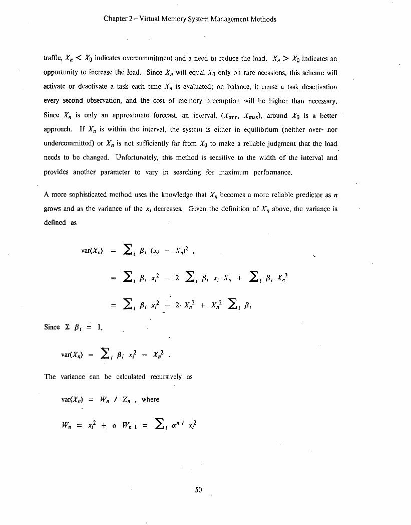
Chapter 2-Virtual Memory System Management Methods
traffic, X,, < X0 indicates overcommitment and a need to reduce the load. X, > X0 indicates an
opportunity to increase the load. Since X, will equal X0 only on rare occasions, this scheme will
activate or deactivate a task each time X, is evaluated; on balance, it cause a task deactivation
every second observation, and the cost of memory preemption will bc higher than necessary.
Since X, is only an approximate forecast, an interval, (Xmin, Xmax), around X0 is a better
approach. If X, is within the interval, the system is either in equilibrium (neither over- nor
undercommitted) or X, is not sufficiently far from X0 to make a reliable judgment that the load
needs to be changed. Unfortunately, this method is sensitive to the width of the interval and
provides another parameter to vary in starching for maximum performance.
A more sophisticated method uses the knowledge that X, becomes a more reliable predictor as n
grows and as the variance of the xi decreases. Given the definition of X, above, the variance is
defined as
var(XJ = xi pi (Xi - XJ2 ,
= CP i i Xi2 - 2 Ci Pi Xi xfl + Ci Pi xtl2
= c i 2 - Xl 2
Since Z pi = 1,
The variance can be calculated recursively as
var(X,J = W,, / Z, , where
+ X?? c i Pi
c
w, = xp + a wR-l = c i an-' * Xi2
50

Chapter 2- Virtual Memory System Management Methods
The variance is exponentially weighted so that it is affected more by recent observations. If we
assume that x is indepcndcnt and distributed normally, we can make the confidence statement
- K var(X,J/n < x < X, + K -jKzy/n ) N- cp ,
where K is the point of the unit normal distribution for which the probability that -K < N(O,l)
< K is also 9.
Even if the xi are not normal, the method is a robust heuristic to determine the variance of the
predictor; load adjustments can be delayed until the predictor has “settled down” and is’ not
dominated by transient behavior. The variance is cxponcntially weighted so that it is affected
more by recent observations.
.
2.3.5 WSCLOCK Load Control
The WSCLOCK replacement algorithm approximates WSEXACI’; it makes periodic scans of each ,
resident page to estimate LR(p) and then applies to the standard WS rule to remove pages from
working sets and make them replaceable. The major difference between WSCLOCK and
WSEXACT is the treatment of non-resident working set pages. When a task is activated, all, or
almost all, of its pages are usually missing. As it exccutcs, the task demands the pages it needs,
which may not include all of the task’s current working set. There may be a number of working
set pages that are about to leave the working set and will not be referenced for some time.
Without the WS scan used by the other WS policies, WSCI,OCK has no mechanism to detect the
departure of these pages; after a number of activation/deactivation sequences. the calculation of
the task’s working set size may be very inaccurate.
If WSCLOCK dots not determine. an accurate working set size, the WS load control mechanism
will be unstable and usclcss. Fortunately, a solution to this problem exists in the proper USC of
the LT/RT control. Consider the state of a task after it has been active for 0 of virtual time.
The WSCLOCK algorithm will have identified, approximately, those resident-set pages that are in
51

Chapter 2-Virtual Memory System Management Methods
the working set and those that are not. AN non-residenf pages are, by definilion, not in the
working set. Thus, 8 virtual time after activation the resident working set is the true working set.
In practice, the resident working set closely approaches the true working set when the loading
phase (as defined by the LT/RT control) has been completed.
Thus, if we define the WSCLOCK working set to be the same as the resident working set,
significant inaccuracy is cxpccted only when the task is inactive or during the loading phase.
When a task is inactive, therefore, its working set size should remain constant and equal to the
value at its last deactivation. To eliminate, or attenuate the effects of, inaccuracy during the
loading phase, we see two solutions. First, we can fix the working set size- to the same value it
had at activation-until the loading phase is complete or until the number of resident working set
pages exceeds the initial value. Second, during the loading phase we can depend on the LT/RT
load control to prevent the WS load control from overcommitting memory. Either solution may
be sufficient; a combination of the two is better.
2.3.6 Demotion-Task Policy
Demotion is a task deactivation that occurs when load control detects overcommitmcnt and directs
a reduction in the multiprogramming level. WC assume that a demoted task is given a special
status and will be reactivated at the first opportunity; not only does this seem to be a fair policy,
it also increases performance to the extent that the demoted task still has resident pages when
reactivated.
We note that a demotion can easily be made to coincide with a page fault. With WS replacement
this occurs naturally since demotion is signalled by a page fault which cannot be processed due to
a lack of uncommitted pages. With global replacement, load control can decide to lower the
multiprogramming level asynchronous to a fault: there is, however, no motivation to select a task
for demotion until there is an event which will alter the allocation of main memory, that is, a
page fault. Although the number of active tasks may bc reduced by attrition, this is unlikely
because lowering of the multiprogramming lcvcl implies that the fault rate is high.
52

rha$rr ?-Virtual Memory System Management Methods
The main issue of demotion is the choice of task to demote. In [DENN80], Dcnning suggested the
lowesf priorify task. Actually, hc suggests that, when overcommitment occurs, the lowest priority
task should give up its pages, one by one, without being demoted until all resident pages are
stolen. This would appear to be a mistake, since the lowest active task will bc forced to execute
with a restricted resident set and will fault often (replacing its own pages) and generate a great
deal of paging I/O without making much progress. In any case, demoting the lowest priority task
may be a proper choice from a policy standpoint, but is not necessarily the best, from a
performance standpoint.
A common suggestion is to demote the faulling task [FoG~74]. This has some intuitive appeal
since there is a greater probability that a faulting task does not have its working set resident, and
performance would suffer least by demoting it. This choice also has an immediate payoff because
it blocks a task which is about to be blocked anyway and it eliminates the overhead of a page
replacement and I/O operation. c
A third choice for demotion is the Zasf fask aclivafed. If the loading task heuristic of the previous
section is employed, the last activated task is least likely to have loaded its working set. Not only
is it the task that executing least cfficicntly (in terms of its page fault rate), it is also likely to have
the fewest resident pages and rcquircs the least amount of effort to reload. For this last reason, a
fourth choice for demotion is the srr~alZcsf task, that is, the one with the fewest resident pages.
Unfortunately, this policy would penalize any program that happened to have a small locality and
should probably be avoided unless it results in a substantial improvement in performance; system
policies should encourage programmers to reduce program locality.
A fifth choice is to demote the largest task; since demotion occurs when memory is
overcommitted, this choice will reduce that overcommitmcnt by the largest amount, making an
additional demotion unlikely. It would appear that the largest task is also the most expensive one
to reload. A counter-argument is that the largest task will lose only enough resident pages to
relieve the overcommitment; if it is the next task activated, it may have most of its working set
still resident. On a policy level, the largest task might also bc thought of as the greediest and that
53

demoting this task would encourage programmers to keep their localities as small as possible. _, -1 w u..’ ,A.%&
Not only is this latter argument narrow-minded, it appears (as shown in Chapter 5) that this
demotion choice has the worst effect on performance
A sixth demotion choice is the task with the largesf remaining quantum, thus effecting a shortest-
processing-time-first scheduling discipline. Finally, random selection can be considered to
distinguish which of the above policies have some sort of positive effect on performance.
2.4 Conclusion
In this chapter, we have described detailed methods of scheduling, memory management, and
load control in a virtual memory system. Numerous new algorithms and techniques were .
introduced. This collection of methods form the basis of the operating system model to be
described in Chapter 4.
54

Chapter 3
Virtual Memory Models
The past 15 years have produced an astonishing variety of virtual memory models. These models
can be generally divided into simpler ones that model an individual program’s behavior under
some virtual memory management strategy, and more complex ones that model a set of programs
being executed concurrently in a virtual memory computer system. Program behavior models can
be divided into stochastic models, which characterize program execution with an analytic or
Markov model, and deterministic models that use a program trace or reference string to drive the
model. System models are similarly divided into analytical models and simulation models. E&h
system model usually incorporates one of the program behavior models.
3.1 Preliminary Assumptions and Definitions
Almost all models of virtual memory decompose the execution of each program instruction into a
set of main memory accesses. Furthermore, each memory access, in the absence of a page fault,
is assumed to require the same time interval to complete. This interval, the reference, is the basic
model time unit. A program is defined by a page-set, P= Ipi 1 i= 1,2,...,m ), and a reference
string, {rt 1 I=1,2 ,..., T }. E&h r, is a pair, 0; p is the page addressed by memory access I; the
boolean d is true if the reference updates (dirties) the page. The integer m is the number of -’
distinct pages referenced and T is the total number of memory accesses.
A residenf sef, R, is the subset of P present in main memory when refcrcncc rI is completed. In
order to execule a program, it is necessary to construct R, at each I such that rt E R, . The
construction is dependent upon the paging algorithm used. The fact that the execution of most
programs can proceed efficiently when R, is only a subset of P is due to the notion of localify: at
a given time, a program tends to reference only a few of its pages and the set of pages being
referenced changes slowly.
55 .

Chapter 3 - Virtual Memory Models
If rt $: R,,, then a page farrlf occurs and a page-in is requited to place rr in R, . Define Ft=l if
a fault occurs for reference f and ‘;1=0 otherwise. Demand paging algorithms never add a page
to the resident set until there is a fault for the page, i.e.,
‘t E v-%1 j F;=l and (RI--Rkl)=rt .
By implication, each reference can cause at most one page fault and page-in.
Let D be the mean page-in delay time. The mean real time required to process each reference is’
RT,,/ (0 = (I+ D FJ,
and the total real execution time is the sum of these
T
RT = 2 RTrti (I). f=l
It is often assumed that the efficiency of a paging algorithm is inversely related to the reti space-
fime producf required to execute a program. The space-time product of each reference is defined
by .
where IR,I is the six of the resident set at time f . The total space-time product is the sum over
all reference times,
T
sTll?d = c I=1
STreJ (0.
Altcrnativcly, we can partition STrCOr into the virtual space-time product and the faulf space-time
product by
T
STvirtuai = c &II f=l
56

: Chapter 3 - Virtual Memory Models
T
sTh”lt = 2 IR,I D Ft . and I=1
Letf be the mean number of faults per reference, (0 < f 5 1). We define the program lijktime, L
= l/f; as the mean reference times between faults.
There are three different measures of memory usage when a program is executed. SvirlUol is the mean virtual resident set size,
sfiulr is the tiean resident set size at fault times,
T
sralllt = STfiurl / IT = 2 ( IRA D F,) h’- l=l
S real is the mean real resident set size,
S real = .sTreal / RT.
57

Chapter 3 -Virtual Memory Models
3.2 Stochastic Models of Program Behavior
3.2.1 Lifetime Models
. Lifelime Curves
The simplest models of program behavior are measured lifetime curves. The execution of a
sample program is simulated (usually using one of the program reference strings described in
Section 3.3) using a chosen page replacement algorithm; the mean resident set, m, and mean
lifetime between page faults, L(m), are calculated and tabulated for different values of nz.
Different values of m arc either generated directly, as with fixed-space rcplaccment, or by varying
a parameter such as 9 for WS. The set of points (m,L(m)) form a “curve.” An idcal lifetime
curve has the convex-concave shape illustrated in Figure 3.1. Below some critical value of m the
program faults very often and L(m) rises slowly. Past this value L(m) increases rapidly until it
reaches a “knee” beyond which additional increases in m have a small effect and the curve
flattens out. Denning [DUNNSO] defines the knee as the point (m,L(m)) that maximizes the value
of the ratio, L(m)/m, and cites studies that associate this point with optimal performance.
Mean Lifetime
I . Kyee , ’
E..
Mean Resident Set
Figure 3.1 - ideal Lifetime Curve
58

Chapter 3 - Virtual Memory Models
Efficient methods for generating sufficient points to produce smooth curves have been devised. : “?G wu Slutz and Traiger [S~uT74] describe a method for generating WS lifetime curves in a single pass
over the reference trace. Dcnning [DENN74] extends this method to VMIN. Bard [BARD73]
measures lifetime curves for global LRU replacement.
Lifetime Funclions
The logical progression from lifetime curves is to lifetime functions. A simple fknction which fits
the points of the lifetime curve is not only a more compact representation but also may indicate
some fundamental aspect of program behavior. Saltzcr [SALT741 proposed a linear function
L(m)=am
where a is a constant, which he observed on the MULTICS system. Dcnning [DENN74] objected
strenuously to Saltzer’s model as unsupportable by existing data.
Belady [BELAYS] suggested a model of the form
L(m)= amk
l
where k is dependent on the locality of the program and is normally in the range [1.5, 31.
Alderson et al. [ALDE71] used the model
in a virtual memory simulation study.
The two previous models model the concave part of the lifetime curve but do not exhibit the
leveling off of real curves. Chambcrlin et al. [CFIAM73] evaulated a model of the form
L(m) = a / [l+ (b/m)2]
which has the desired convex-concave shape.
These fimctions arc only moderately successful in rcprcscnting measured lifetime curves. Actual
program lifctimc curves are rarely smooth and often have scvcral convex-concave regions. The
59

” Chapter 3 -Virtual Memory Models
formulas of lifetime functions cannot be used dependably to infer more subtle properties of e. d (* i 4%
program behavior. There is no basis for assuming that these formulas capture any inherenf
properties of a program’s lifetime curve other than its general shape. For example, Chambcrlin et
al. diflrentiafed the ratio L(m)/(L(m)+ w) to find the value of m which maximized the rate of a
program’s progress. Such a technique is ingenious but perilous, since both the ratio and the
differentiation compound the errors in the lifetime model.
Ambiguily in Lifetime Models
Lifetime curves and functions have become a common method for characterizing program
behavior. As described in the following sections, lifetime models are often incorporated in
computer system models as the sole model of program behavior. In many other cases, lifetime
curves form the basis of more complex program models such as the phase-transition model
described in Section 3.2.5. Thus, we should expect that a given program’s lifetime curve will bc
well-defined and that the method of calculating it should bc relatively unambiguous.
Unfortunately, this is not the case.
We observe that both the choice of page size and the amount of time the program is measured
can drastically alter both the shape of the lifetime curve and the range of lifetime values.
Suppose that a program has m pages and is measured over T references. Since the program
faults at least once for each page, its maximum lifetime is T/m. If either the page size is reduced
by a factor of k, or the measurement period is increased by a factor of k, the maximum lifetime
will be kT/m.
It is not unreasonable for the lifetime to change when the page size is changed, but one should
be careful to choose a page size which is rcprcscntativc of the computer system environment to
be modeled. Q ‘t ft ul c o en, an unrealistically small page size is chosen because the resulting
lifetime curve is more interesting or fits some preconceived notion of what a lifetime curve should
look like. For example, models by Kahn [KA~IN~~] and Simon [Slhfo79] both depend on lifetime
measurements that use a page size of 64 words. Kahn stated that hc “set&d on a 64 word page
60

Chapter 3 -Virtual Memory Models
size . . . because some early analysis showed little sensitivity of program fault characteristics to page
size.” The lower section of the curve may be insensitive to page size, but the upper section is
directly, linearly, dcpcndent on. page size.
It would appear much less reasonable to accept the lifetime curve as a hndamental description of
program behavior when that curve’s upper bound varies directly, linearly, with the amount of
time the program is measured. An analysis of either the Kahn or Simon models using the same
sample programs, but measured for twice (or half) as long as the original sample, would produce
startlingly different results. The fault is not that lifetime curves are difficult to measure, but that
lifetime curves thcmsclves are a weak and poorly-defined model of program behavior.
Another, related, problem with the ordinary definition of lifetime curves is the inclusion of the
initial reference to each page when counting page faults. Most of these initial faults occur early
in the program’s execution and are part of a startup transient which should be eliminated from
the measurement of the program’s long-run behavior. When the mean rcsidcnt set, m, is large,
initial faults dominate over faults due to replacement and are the main cause of the concave part
of the lifetime curve.
Consider, for example, a program which has its entire I;? page address space resident. What is its
expected lifctimc ? The lifetime curve model says T/m, where T happens to bc the amount of
time the program is measured. In reality, the lifetime is infinite because no fault can occur.
Thus, lifetime curves have considerable bias, particularly in the upper sections, past the knee. As
described in Section 3.4.1 and in Appendix A, the results of Simon’s model, which indicated WS *
to be near-optimal, depend almost entirely on the upper sections of the lifetime curves.
We suggest that researchers who build models dcpcnding on lifetime curves consider eliminating
initial faults; of course, the resulting lifetime curves will be knee-less. A number of studies
[KAHN~~, DENNIS, GRAM~~] have associated near-optimal behavior with memory management
policies that attempt to keep a program operating at its lifetime knee. These studies are based on
analyzing system models that incorporate lifetime models of program behavior. If, as this section
61

Chapter 3 -Virtual Memory Models
suegests. the knee is an enhemeral artifact of the program measurement process, these studies * 41 ‘4 + 17t
need to be re-examined.
An alternative to eliminating initial faults is to delay counting faults until a measured program
has executed for some time, thus eliminating the startup transient. We know of no studies in
which either of these methods has been used to remove the bias prcscnt in ordinary lifetime
curves. In Section 5.1, we illustrate the bias in lifetime curves with measurements of real
programs.
3.2.2 The Coffman-Ryan Model
Coffman and Ryan [cOFI72] characterize program behavior by the distribution of working set
sizes: a program’s working set is assumed to vary by a stationary, normal, stochastic process with
mean m and variance 02. The model is validated by analyzing reference strings produced by the
LRU stack model described below, which is itself open to some validity questions. The model is
then used to show that variable-space allocation is better than fixed-space if o2 is relative!y large.
Lifetime curves and functions, and the Coffinan-Ryan model, are not program behavior models as
much as they are replacement behavior models. Replacement algorithms can bc compared to a
limited extent by comparing their lifetime curves on sample programs. Chu and Opderbeck
[GrU72], and Bard [BARD??] have established the superiority of WS and global LRU,
respectively, over fixed-space LRir, but WS and global LRU have not been compared to each
other.
3.2.3 Reference Probability Models
Unlike lifetime models, which simply predict the occurrence of the next page fault, reference
probabilily models generate page references that have some propertics similar to page references
generated by real programs. Each model is paramcterized by the probability vector
m
{ pi 1 i=l,...,m}, c pi = 1. i=l
62

Chapter 3 -Virtual Memory Models
In the Independent Rcfcrence Model (IRM) [AHo~~], each page pi is simply referenced with
probability pr This model only incorporates the fact that some pages arc rcfcrenced more oRen
than others. In effect, it models a program as having a single locality. The parameters of the
IRM are determined by counting the number of references to each distinct page.
Distance string models, or LRU stack models (LRUSM) [SPIR76], incorporate the tendency of
programs to re-reference pages that have been refcrcnced in the recent past. As the program
“executes”, the model maintains a stack of the program’s m pages in order of reccncy of use. At
each reference, r,, the probability that the page in stack position i will be referenced is pf Each
time a page is refcrenccd, that page is moved on the top of the stack, displacing the pages below
it. The process then continues with the updated stack.
Measuring the parameters of the LRUSM is more complex than measuring IRM paramctcrs. As
a reference string is scanned, an LRU stack is maintained and the distance of each reference is
determined by searching the stack. Since most references are to pages near the top of the stack,
the average number of search steps is usually small. Tabulating the frequency of each distance
determines the p;s. The probabilities tend to follow the rule that pi 2 pi+t, but this is not a
hard and fast requirement. If references tend to follow an “instruction, data, instruction, data, ,..I’
sequence, p1 may be quite small while p2 will be larger.
If we assume that the ifs have a natural monotonicity, it is natural (as with lifetime curves) to
look for a simple function to describe them [LEWI73]. Linear, exponential and geometric
relationships between i and pi have been postulated, but this lint of research has little promise.
Both lifetime curves and the LRUSM assume that a program’s locality changes at a fixed rate;
neither models the abrupt locality shifts present in real programs.
63

Chapter 3 - Virtual Memory Models
3.2.4 First-Order Markov Model
In a model of a multiprogrammed system [SEKI~~], Sekino uses a first-order Markov model of
program behavior. The model has m states, one for each page of the program. The transition
probability matrix ( pij ] 1 5 ij 5 m} is defined such that
m
c Pij = 1, for all i. j=l
Each step of the Markov process represents one reference. If the process is in state i at step r,
page pi is referenced; at step 14-1, the process transitions to state j, and references page pj, with
probability pij .
This model is capable of exhibiting abrupt locality changes, but each locality set is fixed for the
duration of the program and may not intersect any other locality set.
3.2.5 Phase-Transition Model
Dcnning and Kahn [DeNN75a] developed the phase-transition model which reflects abrupt
changes in locality. The model consists of a macro-model and a micro-model. The macro-model
is a two-state semi-Markov chain. The states of the macro-model are the phase, in which the
program locality is varying slowly and few faults occur, and the fransition in which the program is
making an abrupt change to a new locality. The micro-model describes the lifetime (or holding
time) in each state. As illustrated in Figure 3.2, the model parameters are:
’ Lphase and Ltransition - the lifetime between faults (holding time) in each state
) pphase and “transition - the probabilities of changing state after a page fault
When the program enters a phase, it executes for an interval with mean $,hase before it
encounters a page fault. Then it enters a transition with probability Z’uansition and remains in the
phase with probability 1- Ptransiuon. Once in a transition, it executes for an interval with mean
L transition (typically ‘Gransition << $Jhase ) and then reenters the phase with probabiiity I)phas@
64 .

Chapter 3 -Virtual Memory Models
P transition
phase
Figure 3.2 - Phase-Transition Model
The paramctcrs can bc specified as various distributions and arc derived by measurement
(KAHN761 or simply postulated [DENN75a]. ‘I’hc definition of phase and transition, as well as the
derivation of the parameters, assumes a prior characterization of locality. In the work by Kahn,
locality is defined by the WS model and the resulting phase-transition model assumes that WS
replacement is used. Modifying this type of model to incorporate some form of global
replacement does not appear to be feasible.
Simon [SIM079] extended the two-state phase-transition macro-model to a three-state model which
includes system-induced program swapping, and then incorporated it in a queucing n&work
model of multiprogramming. WC discuss this model further in Section 3.4.1.
The concepts of phase-transition and the distance string model were combined in the earlier
Shedler-Tung model [SIIED~~]. In their model, a phase is characterized by references with small
stack distances, that is, a small and stable locality. A transition is characterized by a sequence of
references with stack distances of 1+1, 1+2,..., and I+n, where I exceeds the size of the current
locality. Thus, at a transition the model moves n pages from a lower part of the stack to the top
of the stack. The movcmcnt bctwccn phases and transitions is controlled by a Markov model.
65

Chapter 3 - Virtual Memory Models
3.3 Deterministic Models of Program Behavior
3.3.1 The Program as its own Model
The most precise model of a program’s behavior is the program itself. The program behavior of ’
most programs is, in most cases, repeatable at a very fine level of detail. If the program’s origin
remains fixed, relative to a page boundary, the page referencing behavior will also show great
repeatability. .
Canon et al. describe a simulation of VM/370 [CANO~O] that used an enhanced version of the
VM/370 operating system control program. All timing, such as the instruction processing rate
and I/O service times, was simulated to permit the controlled evaluation of various real or
hypothetical hardware configurations under specific loads. The loads that were executed under
the enhanced control program were various collections of real programs.
While appropriate in some instances, this approach has numerous disadvantages. First, it entails
the construction or adaptation of a real operating system capable of processing real programs.
This is a forbidding undertaking for the vast majority of those intcrcsted in performance
evaluation. It is particularly ill-suited for the evaluation of alternative resource allocation and
scheduling strategies; the complexity of most real operating systems makes it exceedingly difficult
to modify the central algorithms.
Without the virtual machine facility of VM/370, which permits the on-line development and
testing of real operating systems, the simulator would be very difficult and costly to implement.
The simulation runs would require stand-alone time on a large-scale machine, which may be
inconvenient, costly, or impossible to obtain. Even with the availability of virtual machines cv
stand-alone time, the real machine used to run the simulation must have a larger main memory
than the computer being simulated. If the simulated virtual system is operating efflcicntly, most
of its simulated main memory is occupied by pages that are active and are being referenced
frequently. Thus, the “working set” of the simulation program will be grcatcr than the ‘size of the
66

Chapter 3 - Virtual Memory Models
simulated main memory. If the real- computer’s main memory is smaller than the simulated
computer’s, thrashing will occur. Further, if the system is simulating a thrashing condition, the
real computer will bc thrashing at a much higher rate. When Canon et al. simulated a 370/145
on a larger 370/168, they were able to run the simulation in a virtual machine. When they
simulated a 3701168 on the 3701168, stand-alone time was required.
Another disadvantage to this approach is the necessity of processing the real workload in addition
to performing all of the operations usually associated with a computer system simulation; not only
do the programs have to be executed, all of the I/O traffic of the simulated system must be
faithfUlly performed by the simulator. This makes each simulation run quite expensive. For
example, Canon et al. simulated a 3701168 computer on a real 3701168 computer; stand-alone
time was required and the real computer run time was 2.5 times the simulated time. This ratio is
considered to be “substantially less than most other types of simulation.”
The simulator was used to evaluate 370 hardware systems using a standard operating system 1 provided for those machines. It was not capable of studying radically different system
management strategies or computer architectures. There was, apparently, no attempt to simulate a
system larger than the real computer available to perform the simulation. Since there is a strong
tendency towards larger and larger main memories, the ability to simulate their effect under
various management policies is an important need that is not feasible with ti~i; Reproach.
3.3.2 Reference String Mod&
The basic alternative to using a program to model its own behavior is to use a truce of the
program. A [race generalor is a program that processes another program by emulating the central
processor functions of instruction fetch and decode, operand fetch, execution, and operand storage
and, at the same time, produces a history, or trace, of the program. The information recorded for
each instruction may include the instruction address, the operation, the operand address(
length(s), and value(s), and the result address and value. Shustek dcscribcs the construction of
such an emulator and its USC to evaluate machine architccturcs [SIIUS~~]. Given a model of a
67

“Chapter 3 -Virtual Memory Models
computer which specifies the duration of each instruction type, the memory access time, cache
structure, address translation overhead and other relevant factors, an extremely precise evaluation
of central processor operation can be performed.
Use of a trace, when compared to the program itself’, has some immediate operational benefits,
The size of main memory used by the simulator drops dramatically. Each page frame of the
modeled system can be represented with a few words; very large main memories can be simulated
on a small computer. All paging and user I/O operations can be simulated without the need for
actual I/O transfers. The complexity of the simulator is sharply reduced, since the need to
support a full operating system is climinatcd, including concerns such as protection and error
recovery. Shustek points out, however, that the trace generator must have explicit knowledge of
the interface between the operating system and the program being traced and, in some cases,
must emulate that interface.
There are several operational disadvantages to using traces. When using traces of programs to
model behavior, it soon becomes apparent that the simple volume of the tract is a considerable
limitation to its usefulness. The disk storage for a few minutes of traced execution may be
prohibitively large. Tape storage may be more cost-effective but will limit the modeling of
multiprogramming to one task per tape drive used. The simulator must read the traces,
generating a significant and costly number of I/O requests. The time to simulate each element of
the trace may be many times the original execution time.
For the purpose of modcling program behavior under virtual memory, these disadvantages can be
reduced by using the simpler, more compact, reference string model presented in Section 3.1. In
this model, program cxccution is modeled as a sequence of memory references, {Q, Q, . ..I. Each
r, is a pair, (p,d); p is the page referenced by memory access I; the boolean d is lrue if the
reference updates (dirties) the page. As the reference string is generated, it is useful to transform
the page addresses isomorphically to the intcgcrs (1, 2, . . . . m}, where m is the number of distinct
pages in the program. Thus, the representation of the page in the rcfcrcnce string is made as
compact as possible.
68
Chapter 3 -Virtual Memory Models
Naturally, we are conccrncd with the nature of errors induced by this simplification. Some
instructions, such as floating-point division, may have an execution time that is disproportionate
to the number of memory rcfcrences. On sophisticated computers, instruction-fetch rcfcrenccs are
often overlapped with execution and references for operand access. In interleaved memory
systems, the access time for multi-word operands is not a simple multiple of the single word
access time. In a system with a memory cache, the pattern of memory references will affect the
mean time for each reference. If a lookaside translation scheme is used, the pattern of access will
also affect the address translation delay. To model these low-level effects would require a many-
fold increase in the complexity and cost of modeling program behavior that, particularly in the
study of virtual memory management, would not improve the model significantly. We shall
assume that these effects contribute to the mean time of each reference but that all references are
identical.
Another source of model error is the indcpendcnce of successive references. In reality, all pages
.referenced during any instruction (by both instruction fetch and operand access) must be resident
simultaneously, so a faithful model would require all references generated by a single instruction
to be processed together. For example, the execution of a single IBM 370 instruction may
reference as many as 8 pages; if a program is being executed in a fixed-space memory allocation
of 7 pages, the independent reference assumption can lead to a considerable error. Fortunately,
this worst case dots not occur naturally, and the overwhelming majority of instructions refercncc
fewer than 4 pages. Further, if a program’s memory allocation were limited to 7 pages (or
otherwise constrained so that the error became significant), the system would be thrashing heavily #.’
and the accuracy of the measurement would have little value.
Finally, one detail of instruction processing, variable length operands, can have a significant effect
on the execution time of some instructions and can be easily retained in the reference string
model. An extreme example is the IBM 370 MOVE LONG, which can access every word of main
memory (either real or virtual) with a single instruction. A straightforward solution is to segment
the operand and gcncratc one reference for each full or partial segment. In oL:r studies, we use a
69

Chapter 3 -Virtual Memory Models
segment size of 8 bytes since this matches the .memory architecture of the class of computers we
are modeling.
3.3.3 Stack Distnncc Strings
In Section 3.2.3, we describe the stochastic stack distance model of program behavior. Each page
reference is characterized by the distance or position of the page in an LRU stack. The stochastic
model assigned a refcrcncing probability to each stack position; the model can be used to
estimate page fault frcquencics for LRU replacement directly or to generate synthetic reference
strings.
The stack distance model can also be used as an alternative representation for reference strings.
Instead of specifying the page being refcrcnccd, each element of the stack distance string specifies
the stack distance of the page. The reduced reference string and a stack distance string are
equivalent reprcscntations of program behavior. For example, the reference ,_ string,
{a,b,c,c,d,c,d,b,d,a}, and the distance string, {1,2,3,1,4,2,2,3,2,4), are equivalent; each can be
automatically derived from the other.
. Since the maximum stack distance is the same as the number of distinct pages, there is no
volumetric advantage to Jhc distance string. (Since the majority of distances are small numbers,
we grant that a variable length encoding scheme may result in a reduction, but at a non-trivial
cost in decoding each refcrcnce.) The main advantage to the use of distance strings would occur
in studies which would otherwise have to maintain an LRU stack of pages. In studies which use
page names explicitly, the overhead of maintaining the stack, required to convert distances to
page names, is a distinct disadvantage.
3.3.4 Filtcrcd String Models
When used to examine realistic virtual memory policies, much of the information in the reduced
refercncc string is redundant. The vast majority of refcrcnces arc to pages that wcrc refcrcnccd in
70

Chapter 3 -Virtual Memory Models
the very recent past. Unless the program’s main memory allocation is unreasonably constrained,
these references will ncvcr cause page faults. We examine two methods described by Smith
[sMIT77] that eliminate redundant information. In Chapter 4, we introduce an improved method
for the same purpose.
Snapshot Strings
i
Reference strings typically have long intervals in which a few pages are repcatcdly referenced. In
such an interval, the actual order and frequency of refcrcnce to each page has a negligible effect
on virtual memory management. Thus the first, and most obvious, technique divides each string
into fixed-length scgmcnts and reduces each segment to a list of pages referenced in the segment.
Let the segment length be w. Define a snapshof at time I,
.
The snapshot sfring is {I,,(o), n=O,I,...,LT/wJ).
.
The snapshot string is easily produced in a single pass of the reference string by simulating the
hardware use and dirty bits for each page. At the end of each virtual time interval, each page
whose use bit is set becomes a reference in the snapshot string; if the dirty bit is set, the reference
is so marked: all bits are reset. A special code, such as (O,truc), is inserted to delimit one
snapshot from the next.
Snapshot strings retain some of the redundancy of ordinary reference strings. In order for the
string to be an accurate model of locality changes, the interval size, w, must be much smaller than
the age of a typical locality set. Consecutive snapshot intervals arc usually in the same locality
and are often identical. The informational redundancy is reduced but not eliminated. Compared
to more elaborate filtering methods, however, the snapshot string is simple and compact.
Smith also determines that lexicographic ordering of page rcfcrcnccs in the snapshot induces an
undesirable bias in the rcfcrcncing pattern; randomizing the order eliminates this bias.
71

Chapter 3 -Virtual Memory Models
.v %tcnnhgllm it ~1 rnnTz73J+devised a similar method, but each snapshot (which is called a loud .* ts -3.
macro) represents a variable amount of virtual time. The snapshot contains a fixed number of
distinct pages; a new snapshot interval begins whenever thd previous snapshot cannot
accommodate the next reference. An elaborate method of simulating the references within a
snapshot was devised so that virtual time could proceed in increments smaller than the snapshot
interval.
Filtered Stack Distance Strings .
Smith observes that most references in the stack distance string are to the top positions of the
stack and can be considered redundant references. He proposes elimination of all references with
stack distances less than a parameter, D. The parameter controls the trade-off between accuracy
and volume reduction. The resulting distance string can then be re-converted to a reference
string as indicated in Section 3.3.3.
Smith distinguishes time-dependent paging policies, such as WS, from time-independent policies,
such as LRU. Study of time-dependent policies would require that each retained reference be
associated with its virtual execution time. We note that realistic multiprogramming models would
invariably require virtual-time information even if the paging policy were ostensibly time-
independent.
Smith compared both snapshot strings and filtered stack distance strings to the standard reference
string in calculating fault rates for fixed-space (LRU, MIN, CLOCK) and variable-space (WS)
replacement. Both methods resulted in a 25:l reduction in trace length with a maximum page
fault error rate of about 7% in the regions of interest. Smaller maximum errors were obtained
when the trace was reduced by a smaller factor.
12

Chapter 3 - Virtual Memory Models
Models of multiprogrammed computer systems fall into two broad categories: analytic and
simulation. Of the many computer system models reported, only a handful have either implicit
or explicit representations of automatic memory management using virtual memory. This section
describes the general failure of analytic models to represent the dynamics of virtual memory
accurately or to provide a vehicle for the comparison of management policies. Simulation
models, while more appropriate for modeling the complexity of virtual memoiy, are usually
simplified to reduce the modeling cost, and suffer from the same problems as analytical models.
3.4.1 Analytical Models
Sekino ‘s Model
Sekino’s model [Se~172] is an elaborate set of analytic qucucing models and other submodels .
representing the physical hardware, system management policies, including memory management,
and program behavior. As will be typical of the analytical models that follow, memory
management in Sekino’s model is severely limited. In particular, the model assumes that: .
1. All programs are identical.
2. Main memory is partitioned equally among the active programs.
3. Each program always makes full use of its memory allocation.
4. Replacement is local.
SekiFo’s model considers only fixed-space replacement, such as LRU, FIFO, and RAND, so that
these limitations are not entirety unreasonable. The necessity for these limitations indicates the
difficulty of extending analytic queueing models to systems that run different programs and have
unbalanced memory partitions.
73

‘Chapter 3 -Virtual Memory Models
Program behavior is represented by the first-order Markov model described in Section 3.2.4. The
system model is used to analyze hardware configurations and to optimize operating system
policies.
Chamberlin’s Model
Chamberlin, Fuller, and Liu [CHAMi’3] provide the only analytic model of virtual system behavior
which does not use queueing theory. It assumes the lifetime model,
44 = a / [l+ (b/m)2]
for program behavior which has the convex-concave shape. By differentiating the ratio
L.(m)/(L(m)+ W’), where W is the page fetch time, a program’s maximum rate of progress relative
to its memory allocation is obtained.
find the optimal multiprogramming
partitions.
Tripathi’s Model
This result is calculated for various memory partitions to
level for a system with identical programs and equal
Tripathi rRIP77] uses an analytic qucucing network model to study virtual systems with a fixed
multiprogramming limit and to compare two fixed-space page replacement algorithms, LRU and
OPT. Program behavior is represented by a lifetime curve derived from measuring real programs
under LRU and OPT replacement for a range of memory allocations. All programs are identical
and receive an equal share of main memory.
The OPT and LRU paging algorithms can be compared by their lifetime functions, . OPT, the
best possible page rcplacemcnt in a fixed memory allocation, generally has lifetimes 50 to 200%
longer than LRU. Predictably, a system with OPT reaches a higher multiprogramming level than
an LRU system before lifetimes become short enough to lower throughput. It is suprising,
however, that the peak OPT throughput is only a few percent better than LRU throughput. OPT
does have a distinct advantage over LRU because it remains near its peak over a wider range of
the multiprogramming level.
74

Chapter 3 - Virtual Memory Models
Simon’s Model
In addition to being the most modern analytic&l model of virtual memory systems, Simon’s model
[SI~MO~O] also incorporates the most complex program behavior model. Further, it is the only
model which is claimed to indicate, albeit indirectly, the relative performance of local and global
replacement algorithms. Thus, we have examined this model in great detail.
Simon constructs a simple queueing network of a computer system having a central processor,
one paging I/O server, and one task I/O server. However, he incorporates an extended version
of the phase-transition model of program behavior described in Section 3.2.5. The extension
adds a third state, swapping, to the macro-model. By considering each of the three states (phase,
transition, and swapping) as a separate customer class, the network is solved using the theorem of
Baskett et al. [BASK’75].
The phase-transition micro-model uses measured WS and VMIN lifetime values for various real
programs. Although VMIN (see Section 2.2.4) is claimed to be an optimal paging algorithtn in
general, it is actually optimal only among local replacement algorithms and then only under
restrictive assumptions. Simon solves the model for various loads and compares WS and VMIN
performance. As reported by Denning [DENNSO]:
Simon compared the optimum throughput from the tuned WS policy to the optimum from the VMIN policy. He found that VMIN improved the optimum throughput from 5 percent to 30 percent depending on the workload, the average improvement being about 10 percent. . . . This is the most compelling evidence available that no one is likely to find a policy that improves significantly over the performance of the tuned WS policy.
a...
Unfortunately, the compelling evidence is illusory. In Appendix B, we include a paper entitled
“Is the Working Set Policy Nearly Optimal?“, which analyzes the Simon’s model and the basis for
concluding the near-optimality of WS. We discuss five major reasons why this model does not
constitute compelling, or even plausible, evidence of WS superiority. For example, it is shown
that the lifetime measurements are badly biased by measuring short rcfcrcncc strings (XC Sections
75

Chapter 3 -Virtual Memory Models
“w -4 *?Tl ml Cl> spd hv ~!c,iy&f small page size. The WS-VMJN comparison dcpcnds mainly on
lifetime measurements where the bias is most pronounced.
Simon’s model is a good illustration of both the strengths and weaknesses of the analytic
queueing model. The customer class concept is a powerful technique that permitted modeling of
the three different states of program behavior. Unfortunately, the qucucing model is unable to
model the dynamics of local memory management faithfully because they require a model load of
statistically identical programs, the equal partitioning of memory, and other unrealistic
assumptions; no one has reported attempting using qucueing models to model global memory
management.
3.4.2 Simulation Models
Most simulation models of virtual memory systems have used crude models of program behavior
to reduce programming complexity and to avoid long, simulation running times. Typically,
memory management is simplified so that the simulator keeps track of only the number of
associated with pages each task and uses random variates to determine when a task will fault or
alter the status of its resident set. -
Alderson et al. [ALDETl] use the lifetime function
L(m)= a2km ,
in a simulation to compare some primitive page replacement algorithms, load control strategies
and paging device organizations. Winograd et al. [wlNO71] simulate a time-sharing system using
a task model that assumes that working sets arc normally distributed and that inter-fault times are
described by the Fine’s curve, which is a precursor of the lifetime models. Bade1 et al. [BADE75]
combine Belady’s lifetime finction,
L(m) = amk,
76

_’ Chapter 3 -Virtual Memory Models
with the assumptions that all programs are identical and share memory equally to study adaptive -* b . .** ~-T&t* f
load control mechanisms.
Chanson and Bishop [CFIAN77] model the M ichigan Terminal System. They recognize that
traditional workload models are not realistic:
In an interactive multiprogram m ing environment, where many resources are competing for lim ited resources, the order in which the demands arrive significantly influences the performance of the system and most resource demand models do not model this well. The problem is in the assumption of the independence of the statistical distributions used. What is needed is joint distributions relating the different variables, but these arc not practically constructable because of the interactions amongst these variables.
They then proceed to model task behavior such that, “page faults are generated from a
distribution ra&er than by a page reference string simulation because of-the costs involved,” and
admit that “[t]his can have an adverse effect on the validity of simulated results in certain areas of
study.”
Grit [GRIl77] performs a simple simulation of two programs competing for memory using global
LRU replacement. Memory references are explicitly generated by a stochastic stack distance
model for each program and it is shown that the program with more locality (i.e., more references
to the top stack positions) pushes the less local program out of memory.
Masuda [M~su77] uses a phase-transition type of program behavior model in a complex
computer system model. Transitions arc predeterm ined by some unspecified process; program
behavior in each phase is specified by a stack distance model with artificially generated
probabilities. The lifetime curve can be derived from the stack probabilities and the need to
simulate individual page references is elim inated.
Gomaa [G0M~79] models the IBM V M /370 system in three different ways: (1) by using the
Bclady lifetime function, (2) by using another lifetime predictor described in [nARD73a] and (3)
by assuming that program paging rates arc known prcciscly. By comparing these models, he
77

Chapter 3 - Virtual Memory Models
concludes that:
The substantial increase in error in the model, when either the [Bclady model] or the [Bard model] is used, indicates that both are crude methods of predicting paging rates.
The folowing two models incorporate explicit representation of pages and frames, and model
program behavior more accurately than the previous system models. They can be considered the
direct antecedants of the model described in this thesis and are used to illustrate the
improvements reprcsentcd by that model.
Nielsen’s Model
Nielsen [NIEL~~, NEL67] develops a finely detailed simulation model to predict the performance
of the IBM 360167 time-sharing system, TSS, on various hardware configurations. The model is
particularly interesting to us because it represents each task page and each main memory frame
explicitly and, thus, has the means of modeling the dynamics of memory managcmcnt under
various policies. The model can simulate the sharing of memory, such as reentrant programs,
between tasks. The model contains explicit algorithms for task scheduling, paging I/O, memory
management, and multiprocessor management, all reflecting the algorithms used in the initial
version of TSS.
Nielsen considers using a stochastic model of program behavior. He rejects the idea because he
considers such a model to be both inaccurate and exceedingly expensive to use as a memory
reference generator. The model he considers would have rcquircd the generation of two random
numbers for each reference. Apparently, he also rejcctsusing measured rcfercnce strings, probably
due as much to the difficulty of obtaining such strings as to their cost when used to drive a
simulation.
The task model used by Nielsen is a set of synthetic program loops. E&h loop contains actions,
typically to reference a single page for some multiple of 100 pscc. The task cycles through a loop
for a number of times and then moves on to some other loop. A set of prototype jobs are
78

Chapter 3 -Virtual Memory Models
constructed by rough judgments of what a typical task would do. As stated in [NIEL~~], “no claim
is made that a prototype represents the behavior of any real job.”
According to the model description, TSS used a primitive local replacement algorithm. A task’s
pages are replaced only if the task was not in the active set. No examination of the use bit, or
any other page activity measurement, is employed and a task’s working set would be all of the
pages it refcrcnced since it was activated. Nielsen uses the simulator to predict bottlenecks due to
paging device performance and main memory size. All of his expcrimcnts predict high system
overhead and generally poor performance. These predictions proved true when TSS was released.
No experiments are performed to compare system resource allocation or scheduling policies
Boksenbaum S Model
The model most similar to the one presented in this thesis is a simulation model of IBM’s CP-67,
a forerunner of VM/370, by Bokscnbaum, Greenberg, and Tiliman @OKS73]. First, the structure
of the model mirrors the structure of a real operating system. Second, the model represents task
pages and main memory page frames explicitly, and manages them as a real iystem would.
Third, the task model is trace-driven, using a reduced form of instruction traces of real programs.
Finally, the model is used to compare replacement algorithms.
The full instruction tracts arc rcduccd to a scqucnce of records called load macros. The
predominant type of load macro Contains the addresses of a fixed number of pages (typically 5 or
10) and an instruction count. The task model proc,esses each load macro by simulating references
to these pages for the specified number of instruction times. Although the method is similar to
snapshot strings (Section 3.3.4), elaborate mechanisms are provided to rcferencc subsets of the
pages for fractions of the spccificd instruction count. Measurcmcnts show close agreement
bctwcen the load macro model and ordinary reference strings when used to simulate FIFO
replacement in a fixed-space memory allocation. Bokscnbaum et al. do not describe the efficiency
of the load macro approach either in terms of refcrcnce string compaction or simulation cost
reduction. WC surmise that compaction is similar to snapshot strings (e.g., 25:l) and that the cost
79

“Chapter 3 -Virtual Memory Models
_, ** rm-hrctinn in sirmlatincr rcferenccs is somewhat less than that due to the elaborate mechanisms to il -,I reference various subsets of the pages in each load macro.
The system model is used to compare two CP-67 replacement algorithms, version 3.0, which uses
global FlFO replacement, and version 3.1, which employs the frame use-bits to approximate
global LRU replacement. Version 3.1 is a marked improvement over 3.0.
The calibration process revealed an important factor in simulating multiprogrammed computer
systems. In both real and simulated systems, very minor changes in some event sequence can
alter the task dispatching sequence and lead to large differences in the measured system
performance. Of course, these fortuitous differences should disappear in the long run, but
extraordinarily long simulationsmay be required to eliminate their effect.
3.5 Conclusions
We have examined an extensive array of program behavior models and computer system models.
The lifetime model may be appropriate for some types of studies, but is too weak and too
ambiguously defined for analyzing the subtle differ-enccs bctwcen virtual memory management
policies. The other simple stochastic models do not appear to bc any better at capturing program
behavior. The phase-transition model is an improvement over the simpler models but it is based
on the lifetime model and inherits much of its weakness. We know of no instance in which a
system model, either analytic or simulation, based on a stochastic program model has been
validated by comparison with a real system or model using non-stochastic program models. Until
such validation is performed, there is little justification for placing confidence in such models.
More precise program models arc more. expensive to use and may have a limited range of
uscfitlncss. An extreme example is the model by Canon et al. which executes programs to model
their behavior. The cost of this approach is extrcmcly high and precludes modcling large systems.
Constructing the model, by modifying an operating system, is also prohibitively expcnsivc. Use
of ordinary rcfcrcnce strings is also expcnsivc since it rcquircs a minimum of 15 to 20 reference
80
Chapter 3 - Virtual Memory Models
/ times to simulaFy,_<:ch rcferencc. Techniques to reduce the rcfcrence string can bring this CI , 48 approach into an economically feasible range; the methods which have been reported previously
can be expected to produce about a 25:l reduction in t&e length with acceptable modelling
error. Since such strings are more complex to use in simulation, we expect to the net cost to be
on the order of 1 reference time per simulated reference.
The analytical system models that are described above have severe limitations. None of them
model the allocation of memory explicitly. Most of them assume that all programs are identical,
that the multiprogramming level is fixed, that page replacement is local, and that memory is
equally divided among programs. These limitations and the models’ dependencies on lifetime
models make it unlikely that they can be used to evaluate memory management politics
effectively. Simulation models which depend on lifetime models and do not represent memory
allocation or page referencing explicitly suffer from many of the same weaknesses as the analytical
models.
We conclude that only a simulation model with an explicit representation of page referencing and
main memory allocation can be relied upon to give trustworthy evaluations of virtual memory
management policies. In Chapter 4, this thesis presents a model that not only uses a highly
accurate model of program behavior and a finely dctailcd model of virtual memory, but also
achieves simulation run times that arc a small fraction of simulated time.
81

Chapter 4
A Simulation Model of a Virtual Memory Computer System
This chapter describes an elaborate, trace-driven, discrete-event simulation model of a
hypothetical virtual memory computer system. The distinguishing characteristics of this model are
(1) a precise, but efficient, model of program behavior and (2) an operating system model.that is,’
for all intents and purposes, a finely-detailed facsimile of not one, but many, different operating
systems.
Program behavior is modeled with a new, trace-driven, Inter-Reference Interval Model (IRIM)
which is several orders of magnitude more cfflcient than the reference string model, but which
has a negligible loss of accuracy. The IRIM makes practical the precise simulation modeling of
virtual memory management and, in many cases, is preferable to analytical models. 5
The operating system model, while comparatively simple in design, incorporates many different
strategies for scheduling, memory management, and load control. It permits the direct
comparison of local and global memory ‘management policies; coupled with the IRIM, it also
permits precise calculations of the task-working set (impractical on standard computers) and the
optimal, lookahead, algorithm, VMIN. All of these capabilities arc implemented so as to
eliminate superficial implementation disparities and allow a comparison of their essential
differences.
Section 4.1 describes the basic methodology, structure, and implementation of the model. Section
4.2 dcscribcs the configuration model which dcfincs the hardware elements of processor, main
memory, and I/O devices. Section 4.3 describes the task model, including the definition of the
IRIM and its use to model memory referencing. Section 4.4 describes the operating system
model.
. ::p
* -. ,*-., -
.’ .,
82

Chapter 4’- A Simulation Model of a Virtual Memory Computer System
4.1 Introduction
The methodology of discrete-event simulation modeling is well established. We have depended
heavily on the excellent texts by Fishman [FIsIJ~~], Shannon [SIIhN75], and Klcijnen [KLEI75],
and refer the rcadcr to them for more detailed accounts of the methods used in this work.
4.1.1 Simulator Construction -
_
The basic structure of the simulator is shown in Figure 4.1. There are four major components.
‘IQ input processor accepts statements in a simple, free-form specification language described in
Appendix A. These statements can cause the loading of previously created files of other
statements, such as standard configurations, workloads, and system parameters. The input
pr&essor creates data structures to represent the various objects, such as main memory, tasks, and
I/O devices, which comprise tic system configuration and workload. The inilializalion processor
checks the generated data structures for consistency, assigns default values for unspecified options,
and generates a prc-simulation report.
The execution processor, which is described in the following sections, performs the simulation. It
accesses files of program traces (reference or IRIM strings) to drive the task models. As the
simulation proceeds, samples of processor utilization and detailed operation traces can be
generated. The reporf generator analyzes and displays the results of the simulation and resets the
simulator to accept a new set of specification statements. The summary report of a typical
simulation is reproduced in Figure 4.2.
,
The simulator is programmed in HIBAL, a medium-level, block-structured, system
implcmcntation language. It has 5400 lines of source code and occupies about 30,000 bytes of
storage, exclusive of dynamically allocated data structures and I/O buffers. It required about l/2
person-year to design, write, and debug.
83

Chapter 4 - A Simulation Model of a Virtual Memory Computer System
Input I Program Traces
Standard Configurations and Workloads
‘I
Input
m--i
Processor
Initialization
Processor
Pre-simulation Report
b
Execution
Processor
Sampling Tracing
4
Report Generator
Report I/
Figure 4.1 - Simulation Program Structure
84
F
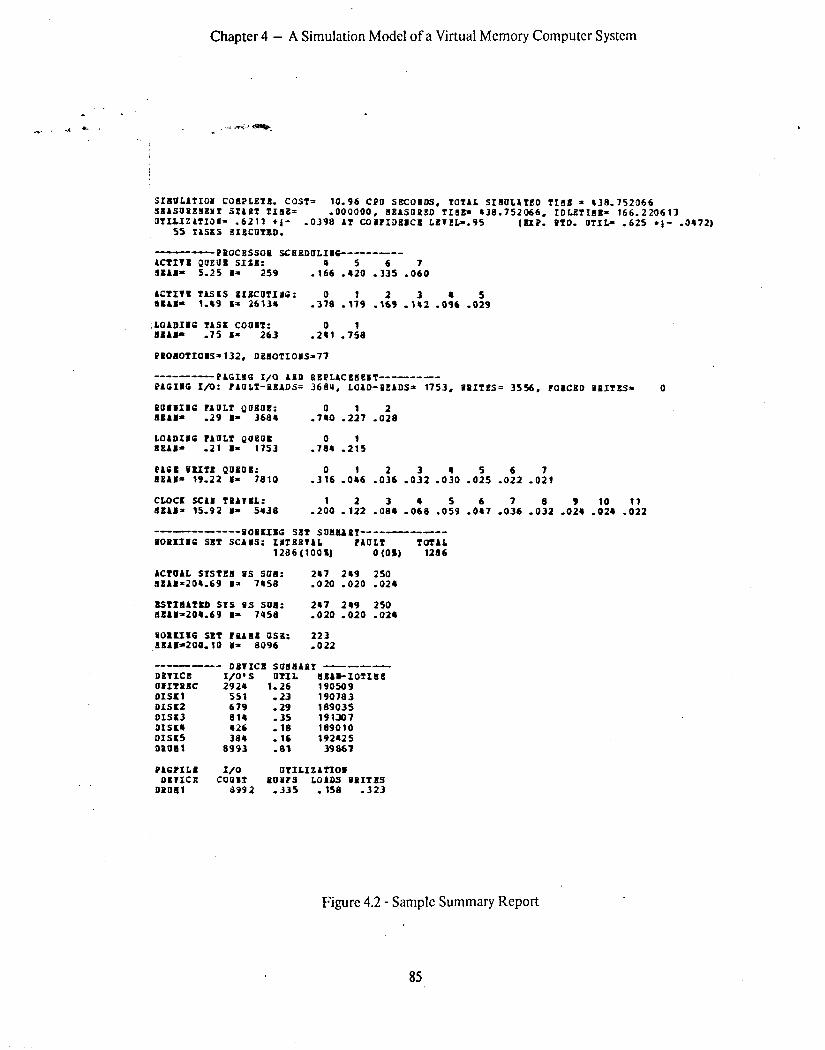
Chapter 4 - A Simulation Model of a Virtual Memory Computer System
SXiAIJLATIOl COEPLBTI. COST= 10.96 CPU SECOIDS, TOTAL SIIULATEO TIIX = 438.752066 aKAsuPzaBYr STAilT TInz= .oooooo, IIBASUPBD TIE- #38.752066, LDUTIlK= 166.220613 0TUIZATIJI= .6211 *I- -0398 AT COI?IDBICI LBV‘LL=.95
55 TASES BIBCUTBD. (UP. WTD. ‘.lTIL= ,625 +I- -0472)
----PPBOCESSOD SCEBDULIIC-------- ACTITI QOEUB SIZI!: 0 5 6 7 Jail= 5.25 I= 259 a 166 .420 .335 .060
ACTIIK TASL5 OIBCUTIE6: aus- 1.49 I= 26134 .3:FI .I:9 .lt9 .I:2 .0:6 .0:9
LOADImC TASK COOaT: 0 IllAl- -75 I= 263 .2Ql .7:e
P1OIOTIOIS=132, D810TIOBS=77
--------PAGIYG I/O LID ESPLACKaEllT-------- PAGIIG I/O: ?A9LT-READS= 3684, LOAD-READS= 1753, l lPITES= 3556, ?ORCXD @PITKS= 0
P'JHU16 ?A'JLT QtlBOE: EEAH- -29 I- 3684 .7:0 .2:7 .0&l
LOADABE ?AULZ QUEUE 0 1 1KAB’ -21 I= 1753 .784 -215
PAEl rura Qoeoa: 0 1 2 3 agAB= 19.22 I= 7810 .316 -016 .036 -032 .OfO .OiS .Of2 .Oh
CLOCX SCAI TPAIEL: 1 ItAl= 15.92 I= 5438 .200 2 .Oh .Ote 5 .Ot7 7 8 9 .122 .059 ,036 -032 -024 10 .::2 -021
---------POPl(f,G Slf SD,,~pT--------- IIOPXIIE Sll? SCAlSr IITBXTAL IAULT TOTAL
12’36(1001) 0 (OS) 12S6
ACTWAL srstza ws SOI: 247 219 250 EXA1=201.69 I= 71)58 .020 .020 .024
8STIEATXD SrS IIS 5011: 247 249 250 lKA1=204.69 I= 795% .020 -020 -024
UOPUMG SET PMaZ ‘JSB: 223 IEAPZOQ. 10 I= a096 -022
-- ‘-- DPTICE SOEIAPT --me- DBTICE L/O’ s OTIL ISA+IOTIllB OiIY!illC 2924 1.26 190509 01sc1 551 -23 190783 DISK2 679 -29 189035 DISK3 814 -3s 191307 DISC8 b26 -18 189010 DISKS 384 16 192425 DPDIIl 0993 :a1 39867
PAGIXLE f/O UTILXZATIOI DillICE COUlJT POWS LOADS PPITl1S
DPUSl a99 2 ,335 . 158 -323
Figure 4.2 - Sample Summary Report
85

Chapter 4 - A Simulation Model of a Virtual Memory Computer System
4.1.2 Verification
Fishman [FISH731 identifies a number of circumstances which may cause a simulation to fail to
agree with the underlying model:
) A poorly chosen pseudo-random number generator
) Inappropriate approximate random variate generation techniques
) Input parameter misspccification
) Programming errors
) Measurement errors
We shall consider each of these in turn.
Pseudo-Random Number Generation
The simulator uses the multiplicative pseudo-random number generator
ri = 7’ ri-1 modulo 231 - 1,
which has a maximal period of 231 -1. ‘Ihis generator is suggcstcd by Lewis, Goodman, and
Miller [LEwI~~]. It has been checked using a variety of statistical tests by Lewis et al. and, more
recently, by Fishman [FISHES]. Although it does not pass ali tests, it performs well in comparison
to the other commonly used generators.
Each simulated random process, such as a task cxccution or an I/O dcvicc, is provided with an
indcpendcnt stream of pseudo-random numbers. Each process uses the same generation formula
but maintains its own generation seed. Initial seeds for the indepcndcnt generators are
themselves generated with the mixed congrucntial generator,
Si = (314159621 SKI + 1) modulo log,
86

Chapter 4 - A Simulation Model of a Virtual Memory Computer System
suggested by Knuth [KNUT69]. By using a seed generator of an entirely different type, we avoid
introducing any systematic overlap between pseudo-random number streams. In order to test the
simulation’s sensitivity to the randomness of the stochastic components, the seed of each
component’s generator, as well as the seed of the seed generator, can be specified explicitly.
Random Variate Generalion
The pseudo-random integer ri is converted to a real number uniformly distributed on [O,l) which
is used to produce integer-valued samples ‘of four distributions: constant, uniform, exponential,
and truncated exponential.
Table 4.1 - Random Variate Specification
Parame tcrs Dlstrtbutlon Value
min constant min
min= max constant min
min = mean constant min
min = mean = max constant min
max
min< max
uniform
uniform
S(l,max)
S(min,max)
mean
min< mean
exponential
exponential
1+ E(mean- 1)
min+E(mean-min)
min<mean<max truncated exponential min(min + E( mean - min),max)
means max truncated exponential miri( 1 + E(mean - l),max)
The type of distribution is specified implicitly with three parameters: min, mean, and max. Only
a subset of the parameters need bc spccifkd, but it is required that l~min<mean.<max. Table
4.1 gives the distribution implied by each legal combination of parameters. S(a,b) is a sample of
the distribution in which the integers a,a+l,..., b, are chosen with equal probability. E(a) is a
sample of the cxponcntial distribution with mean a, rounded to the ncarcst integer.
87 l

Chapter 4 - A Simulation Model of a Virtual Memory Computer System
The gcncration of the constant distribution is. trivial. The generation of S(a,b), on [a,b] from a cp -t- I ..a,*-
umform random number, u, on [O,l) is straightforward:
S(a,b) = Lu (b-a+l)J+a.
The generation of a non-uniform distribution, such as an exponential distribution, can be ’
performed with the inverse transfom?ational method. If x is a random variable with pdf f(x) and
cdf F(x), then x is a random sample of x if
s
X
Prob[x<x] = F(X) = fcv) dr -00
is uniformly distributed over (OJ). That is, if u is a sample of U(O,l), then x, such that F(x)=u,
is a sample of x. Since the pdf of the exponential distribution with mean A,
f(x) = l/h emxiX for ~20,
f(x) = 0 for x<O, .
is integrable, F-l(x) can be evaluated directly:
I X
u = F(x) = l/h e-v/Ad, = * -e--Y/A - l-e-X/h , 0 0- .
e-X/X = l-u,
X = -A ln(l-u).
If u is U(O,l), then so is l- u, and
E(a) = -a In(u).
Simulalion Inpul Specificution
The simulation input parameter specification language is described in Appendix A. The format
of the language is dcsigncd to minimize the possibility of accidental misspccification. Input
88

Chapter 4’ - A Simulation Model of a Virtual Memory Computer System
parameters that arc common to a set of simulations, such as the configuration and workload, can.
be stored in a file and accessed with a single input statement. Thus, errors due to mistakes in
duplicating a standard environment are easily avoided.
Following the input phase, a pre-simulation report is generated. This report describes the
configuration, workload, and system options in effect for the simulation run. It is a simple matter
to check this report for agreement with the intended input specification.
Programming Errors
The problem of detecting and eliminating programming errors is one which pervades the use of
computers in any endeavor; we have no special methods of attacking the problem. Even if WC
were able to validate the simulator by comparison with real systems or indepcndcnt models, there .
is no guarantee that some new combination of input specifications would bc processed without
error.
As the simulator was programmed, numerous tests were included in logic sections that would
otherwise continue to function in the presence of errors. There was also a conscious effort to
eliminate programming robustness; .it is desirable that any errors propagate themselves and cause
obvious output inconsistencies or outright failures.
The simulator has an extensive execution trace capability that records a selectable set of simulated
events such as task scheduling, page replacement, load control, etc. The detailed operation of the
simulator was examined at a very low level for accuracy and consistency. Numerous
programming errors were detected and eliminated by use of this facility.
Measurement Errors
Verifying the accuracy of the performance measurement is a difficult task. WC have examined
the output of hundreds of simulation runs of varying length and complexity, and have ensured
that the output has face validity. The simulator has been tested with parameter sets that have
89

Chapter 4 - A Simulation Model of a Virtual Memory Computer System
extreme values; the behavior of the simulator has been consistent with the generally expected
behavior of the modeled system.
Some consideration was given to comparing the behavior of the simulation model to an analytic31
model or to a real system. The fundamental reason for using simulation is to represent the
dynamic program behavior and complex memory management interaction which arc beyond the
capability of any reasonable analytical model. In fact, we would consider it more appropriate to
use the simulation model to analyze the errors and lack of faithfulness in such analytical models.
.
An attempt, by the author, to study a real computer system, with the intention of comparing its
behavior with that of the simulator, has only scrvcd to illustrate the usefulness of the simulator.
It was impossible to obtain reproducible results on the real system due to the vagaries of the
physical devices and the difficulty of controlling the scheduling processes in real operating system.
In real systems, very small perturbations in time lead to large differences in measured
performance. The work of Canon et al. [cANO79], dcscribcd in Chapter 3, illustrates the
complexity and expense required to achieve reproducible results with a real system.
4.1.3 Model Structure
Descriptions
The significant elements of the mod& particularly the program behavior and memory
management models, are described in considerable detail, both in ordinary prose and by program
fragments. These fragments have been taken from simulation code, omitting pedestrian details
and translating the implementation language to one resembling Pascal. Although thcsc fragments
are faithful reprcscntations of the simulation processing, the rcadcr should be warned that they
are not verbatim and have never been compiled or executed.
Program fragments, while not the most elegant way to convey information to the reader, perform
three important functions. First, they arc precise descriptions of the model. Our a!tempts to
90

Chapter 4 - A Simulation Model of a Virtual Memory Computer System ’
understand many previous studies have often been frustrated by a high degree of abstraction and __ . -4 *i I .’ ‘L %.e.
? . omission of important details of the modeling process: thus, we have tended to provide an
unusually high degree of detail for those who might wish to understand or extend this work.
Second, the fragments serve to illustrate the relative simplicity of the algorithms used to model
_- the computer system and to increase confidence that the model has been implemented correctly.
Finally, they may bc useful to both operating system designers as well as the simulation
practitioner: they demonstrate that it is practical for very different (e.g., local and global memory
management) strategies to be implemented simultaneously in the same operating system.
Time and Clocks
Time is measured in discrete multiples of a single memory reference time. The system real-time
clock measures the passage of total or “wall clock” time. Each task has a virtual-time clock which
measures the number of references successfully completed.
. On typical modern computers, the average reference time ranges from tens of nanoseconds to
scvcral microseconds. Thus, all times expressed in the model are relative to the speed of the
processor. To simplify the following descriptions, we assume a standard reference time equivalent
to one microsecond. When the simulator is parameterized to model a particular computer, all
other time values arc scaled appropriately.
. In this model, we do not simulate overhead. The real-time clock is advanced only when a
reference is successfUlly processed or when the system is idle. The inclusion of overhead in the
model is not difficult and would make an interesting followup study, especially in light of the
results of Chapter 5. Our intent in this study is to measure the essential difference between
alternative strategies without clouding the results with the effects of overhead.
Events and Interrupts
The simulation model is event-driven. Events are specific actions which the simulator is to
perform at some fixture real time. ‘1%~ simulator maintains an EvejrtQueue which is a list of
91

Chapter 4 - A Sitiulation Model of a Virtual Memory Computer System
Event records as shown below. The Even/ records are ordered by the time they are scheduled to
occur. When the system is busy (i.c., processing program references) the real- and virtual-time
clocks are updated until the real-time clock equals the time of the next scheduled event; then an
interruption occurs. Whenever the system has no work to perform, it idles until the next event.
Idling is a simple and efficient matter of advancing the real-time clock to the time of the next
event.
type Event = record Next: t Event; {EvenfQueue link) Time: lime; {scheduled real time of event} Action: proccdurc {called when event occurs)
end ;
Submodels .
The model is conveniently described as a set of three submodels: the configurufion model includes
the basic hardware (processor, memory, and I/O devices) and fundamental concepts such as time;
the fask model represents the execution of programs as a sequential memory rcfcrencing and I/O
requesting process; the operating system model performs the functions of allocating hardware
resources in order to execute tasks. While the configuration model and task models are simplified
versions of their real counterparts, the operating system model is a detailed replica of the central
allocation and scheduling mechanisms of a real system.
4.2 Configuration Model
4.2.1 Processor Model
This model contains no explicit representation of the processor. The operations normally
associated with a processor, such as task execution, arc performed as part of the other models.
92

Chapter 4 - A Simulation Model of a Virtual Memory Computer System
4.2.2 Main Memory
Main memory is a collection of frames, each of which can contain a single page. The size of a
frame or page is not specified but is implicitly characterized by the task model. The content of
each frame is irrelevant and requires no representation in the model or storage allocation in. the
simulator. Each frame is identical and can be assigned to contain any task page. The memory
required for the operating system is assumed to be fixed and suplemental to the memory
represented in the model. Each frame is represented by the following data structure: . type Frame = record
{hardware functions} Use, {page has been referenced} Dirty: Boolean; {page has been modified} LastReferenceTime: lime: {special hardware capability)
{memory management functions) Free: Boolean; {does not contain any page} Owner: t Task; VirtualAddress: t Page;
(paging I/O control functions} Next, Previous: t Frame; {paging I/O queue links) PageIn, PageOu I: BooZean (paging J/O status}
end;
and main memory is a fixed array:
const MemorySize = 250; var MainMemory: array [l..MemorySize] of Frame;
Associated with each frame are the Use and Dirfy bits which are commonly found on virtual
memory computers; these are set when a page is referenced or changed, respectively, and are
cleared by the operating system.
Under the WSEXA~ replacement algorithm, the variable LasfRefercnceTime is modeled as part
of the configuration model- a hardware register is updated automatically, each time the frame is
rcfcrenccd. For the other replacement algorithms, LasfReferenceTime is a sim,plc software entity
that is the operating system’s approximation of the last time that the frame was referenced.
93

Chapter 4 - A Simulation Model of a Virtual Memory Computer System
The remaining variables associated with each frame are software artifacts that are maintained and
used by the operating system, and are described in Section 4.4.
4.2.3 I/O Suhsytcm Model
In direct contrast to the level of detail used in simulating memory and processor management,
I/O devices arc modeled very simplistically. In real systems, many factors contribute to the time
required to complete an I/O operation. The operating system must interpret, verify, schedule,
and initiate each I/O request. Queueing delays for obtaining an access path depend on the
processor-channel-controller-device configuration. The operation itself is subject to seek and
latency delays; the transfer time depends on the device speed and the length of the data record.
I/O completion requires processing to detect errors, release the access path, and schedule the
waiting task for execution. Realistic modeling of device access time should also consider serial
correlation of sequential file accesses and the lack of correlation for random accesses.
In the study of device scheduling policies, optimal hardware configurations, etc., some or all of
these factors should bc modeled faithfully. In our study of virtual memory, the I/O device model
is intentionally simplified so that its effect on system performance is uniform. The elimination of
perturbations caused by the physical details permits a clearer focus on the memory management
policy questions that are studied in this work.
The following data structure describes the characteristics of each device:
type Device = record BUSY, Serial, Boolean; Queue: T IORequest; (unproccsscd requests} .MinIOTime, Mean IOTime, MaxIOTime: time; Seed: infeger {random variate seed}
end;
94

Chapter 4.1 A Simulation Model of a Virtual Memory Computer System
.a c Far-h dpvicp is rn~~rklecl as an independent entity which operates in parallel with the processor cc . . _. and other devices. When scheduling of I/O devices, the operating system model which processes
requests for both task and paging I/O in the same way. Each request specifies a particular
“&vice, and is either processed immediately or is placed in the device queue for processing when
the device is available. When a request is completed, a simulated interrupt tansfcrs control to the
operating system. t
A device which is designated as Serial can process a single I/O request at a time; the queue of
pending request.s is processed in FIFO order. Otherwise, a non-Serial device can process any
number of I/O requests concurrently. This capability is use!%1 for modeling an entire terminal
system with a single device. The service time of the device is independent of the requesting
entity and is modeled stochastically. Access time distributions can bc specified as constant,
uniform, or exponential. .
4.3 Task Model
The task model consists of the general task state, the virtual memory state, and the execution (or
program behavior) model. Execution is modeled as a sequence of memory references punctuated
by stochastically-generated I/O requests. Memory references are generated by a trace-driven
model such as the rcfcrencc string or IRIM. Task termination occurs deterministically when the
reference string is exhausted. Figure 4.3 provides an overview of the task model.
,
95

Chapter 4 - A Simulation Model of a Virtual Memory Computer System
0 Initiation
Reference String I I I I II I I I I 11 1
f(p,d)
-0 Tergi;a- .
Figure 4.3 - Task Model
4.3.1 Task State
The task state is dcscribcd by the following record:
type Task = record {virtual memory state) PageTable: array [ 1.. h/laxPage] of Page: WorkingSefSize: l..MaxPage; WSScanTime: he;
96

Chapter 4’- A Simulation Model of a Virtual Memory Computer System
{execution state) VirtualTime: lime; {ReferenceShingModel;) NexUOTime: integer,
{I/O request model) MinInterIOTime, MeanInterIOTime, MaxInlerIOTime: integer, DeviceUse: array [l..MaxDevice] of real; CurrentDevice: t Device; Seed in leger,
{scheduling state) Active, Ready: Boolean: Blocked: Boolean: WaitingForFrame: Boolean; Loading, Swapin: Boolean: QuirnhtmEnd: lime; Lasl WaitTime: time: RealAclivationTime, VirlualActivationTime: lime
end;
4.3.2 Virtual Memory State
The task’s virtual memory state is described by a PageTable array, which contains a model of
each task Page, and a number of state variables maintained by the operating system. Each Page
’
is modeled by the following data structure:
type Page = record RealAddress: ? Frame; Resident: Boolean: {page is resident) Slol Address: inleger; In WorkingSet: Boolean; {used by replacement algorithm) LastReferenceTime: time; {used by replacement algorithm) IRIbusy, IRIdirly: Boolean; {used by IRIM)
end;
97

’ chapter4 - A Simulation Model of a Virtual Memory Computer System
In a real system, a PageTable element usually contains only the RealAddress of each resident page _ .i *\ -.+L1*i
/II a minimally coded format. Since the address of each frame is constrained, by the hardware, to < being a multiple of the page size, the address translation hardware dan transform a relative frame
pumber to the actual memory address of the frame. In the model, since no memory is actually
allocated for the frame or the page, the RealAddress is simply a pointer to the data structure tiscd
to model the frame. The Residenf boolean variable in the Page element signals the model of the . @dress translation hardware that a page is or is not resident.
The SlotAddress contains a coded description of the page’s location in auxiliary memory. This
model, however, dots not manage auxiliary memory explicitly and this elcmcnt is largely unused.
The elcmcnts In WorkingSet and LastReferenceTime are maintained by the replacement algorithm
being modeled. ZRIbusy and ZRIdirly are special indicators used only for the simulation of the
IRIM of program behavior and are not usually represented in a real system.
4.3.3 Inter-Reference Interval Model
Introduction
In this section, we introduce the Inter-Reference Interval Model (IRIM) of program behavior.
The IRIM is a deterministic, trace-driven, model of the program reference string that is used to
simulate virtual memory referencing. The IRIM is derived by a computational procedure that,
compared to the processing required to collect the original reference string, is efficient and
applicable to very long strings. When used to study modern virtual memory management
strategies, the IRIM is an accurate and efficient method for modcling program behavior.
The cffcctivcncss of the IRlM is based on the cxistcncc of program locality and the behavior of
practical memory management policies. Locality implies that, at any given time in a tasks’s
execution, most program pages fall into two groups: those that are being referenced frequently
and those that are not being referenced at all. We consider a practical rcplaccmctit algorithm to
be one that rarely or ncvcr replaces a page that is being referenced “frcqucntly”, unless the task
. .
98

Chapter 4 - A Simulation Model of a Virtual Memory Computer System
that owns the page is deactivated. In the IRIM, frequenfly is defined to mean “at least once every “* *r). u references”, where o is a model parameter similar to the WS model parameter 8. At each
point in virtual time, the IRIM divides the task’s pages into a busy set and an idle set, such that
the busy pages are being referenced frequently and the idle pages are not.
Since the need to clean dirty pages before replacing them has an effect on performance and,
further, since there are alternative cleaning strategies to be evaluated, a program model should
also provide information about the nature of page dirtying. The IRIM divides the set bf busy
pages into clean pages and dirty pages: a dirty page is one which is being updated at least every
0 references.
Although the IRIM is similar to the WS model, in that a page not referenced for w (0)
consecutive references will be removed from the busy (working) set, there are several important
differences. If r, and r,, are two successive references to the same page, such that u-f 2 o (or
2 8), the IRIM removes the page from the busy set immediately after r,-at time I+ l- while . WS removes the page from the working set at time t+8. The IRIM also distinguishes page
changes from simple accesses; it even models the fact that a page may bc first changed, then
simply accessed for a time, and- then changed again without passing through an idle period.
. Formal Definition
We describe the IRIM formally as ‘follows:
Let P = Cpi 1 i=1,2,..., m} be a task’s page set and (rl 1 1=1,2,...,T) be its reference string as
defined in Section 3.1. Let I, C, and D be three mutually-exclusive sets of page-time pairs (p, I)
from P X {1,2 ,... T) such that P X (1,2 ,..., 7’j = I U C U D. The clcments of each set are
defined by the mapping
@,,: P X Il.2 ,..., 7’j --, {I, C, D},
99

Chapter 4 - A Siinulation Model of a Virtual Memory Computer System
where: 1) QD, b, I) E C U D iff there exist a 11 and (2 such that:
ai 11 I ( 5 (2, b) ql = rt2 = p , and c) f1- (2 5 w;
2) Q>, @, I) E D iff there exist a 11 and 12 such that: a) 4 5 I 5 (2, b) rq = rQ = (p, (rue), and c) tl-12 5 w.
The three sets contain page-time pairs that arc idle (I), clean (C), and dirfy (D). For convenience,
we define a new set B, 13 = C U D, containing busy pages. Thus, at time I, page p is idle if f is
in some interval [fl, fd of at least w references and p is not referenced in the interval; otherwise p
is busy. Likewise, if p is busy, it is also clean if I is in an interval [II, f2] of at least o references
and p is not modified in the interval; otherwise p is dirty. .
Next, we define the set II by
11 = cp I %&I (P, 0 E 1 3,
which contains all idle pages at time 1. Cl, D,, and Bt are defined similarly. At time I, we refer
to the triple {I,, Cl, DJ as the model state St.
To represent the IRIM by’ recording St for each t is both impractical and unneccessary. Due to
the locality of refcrenccs, pages are either busy or idle for long periods. They arc also, in the
IRIM sense, either clean or dirty for long periods. Thus, for practical values of w, there are
relatively few times f when SI Z S,+ 1. When successive states S1 and St+1 are not the same,
there are at most two pages (p= rf and p’= r,+L) which change sets:
1) p moves from C, or I), to I,+1 if p 4 {rr+l,...,rr+ w}; or
p moves from Dt to Cr+l if p is not dirtied in {rl+l,...,r,+,3.
2) p’ moves from It to CI+l or D,+ 1 if p E II; or
p’ moves from CI to D,+l if r(+l is a dirty reference.
100

Chapter 4 - A Simulation Model of a Virtual Memory Computer System
In Section 5.1.3, it is shown that, for practical values or U, S changes infrcqucntly; a compact
representation of the IRIM, known as the IRIM string, is a sequcncc of transition records that
specifies each change to S. These records have the forms:
(4 P, “I”, 4 - p is idle in [I, I+ n) (t, p, “c”, 0) - p is clean in [t, I + n) (t, p, “D”, n) - p is dirty in [I, t+ n)
The records are ordered by time I. The fourth element, n, is the tenure of the page in a particular
state; it is used to predict the next trahsition of a page for lookahead algorithms.
IR IM String computation
The computation of the IRIM string has two processing steps. In the first step, transition records
are produced in a single pass over the reference string. These records are only partially time-
ordered and must, in the second step, be sorted by time.
As each reference is processed, the state of each page p is defined by three variables:
) Start (p) - last time page entered either the C or D set,
b LastUse (p) - time of latest reference to page, and
b LastDirty (p> - time of latest page change.
Immediately prior to processing reference I, the following relationships hold for each p: +
b I- Last&e (p) 2 id =+ p is idle in the interval (LastUse (p) + 1, t - 1)
b LastDirty (p) < Start (p) * p is clean in the interval (Start Q, LastUse (p))
b Start b) 5 LastDirty (p) * p is dirty in the interval (Start (p), L,astUse (p))
101

Chapter 4 - A Simulation Model of a Virtual Memory Computer System
When executed for each reference (p,d) in the original reference string, the following program
fragment creates the IRIM transition records.
if I - LastUse (p) 2 w then {page has completed idle state}
begin if Start (p) 5 LastDirfy (p) then {previous state is dirty}
write (Start (p), p, “D”, LastUse (p) - Start (p) + 1)
else wrife (Sfarf (p), p, “C”, LasfUse (p) - Start (p) + 1);
write (LastUse (p) + 1, p, “I”, I- LastUse (p) -1;
Start (p) : = t
end
else begin {p g a e not idle; check for &an/dirty transition)
{dirty reference may signal a clcan+dirty transition}
if d and (LasfDirfy (p> < Starf (p)) and (I - Sfart (p) 2 w) then
begin wrife (Sfarf (p), p, “C”, I - Sfart @));
Sfarf (p) : = I
end; .
{clean reference may signal a dirty-clean transition}
if not d and (Sfarf (p) 5 LasfDirfy (p)) and (LasfDirfy (p) - I > w) then
begin write (Sfarf (p), p. “D”, LasfDirfy (p) - Sfarf (p) f 1);
Sfarf (p) : = LasfDirfy (p) + 1
end
end;
LastUse (p) : = t;
if d then LastDirty (p) := t;
Briefly, if two succcssivc rcfcrcnccs to a given page arc at least w rcfcrenccs apart, we know that
(1) a busy state terminated at the time of the first reference, (2) an idle state occurred during the
interval between the rcfercnces, and (3) a new busy state began at the second reference. Records
that describe both the previous busy state (either clean or dirty) and the idle state are written to
an output file.
102

Chapter 4‘- A Simulation Model of a Virtual Memory Computer System
If a page is referenced in a busy state, it is tested for a C * D transition. This occurs whenever . . . ar r~.%-~~
(1) a dirty page remains busy but is not dirtied for w or more references, or (2) a page receives
only clean references for w or more references and is then dirtied. When a C ;FI D transition
occurs, any time between the states (i.e., after the last clean reference and before the first dirty
reference, or vice-versa) is included in the C state record. Thus, the exaggeration of page dirtying
in the model is minimized.
An additional mechanism detects the first reference to each page and avoids generating records
for the period before that reference. When the reference string is exhausted, records are written
for each page to describe a final return to the idle state.
Although the records for each page are produced in time-sequenced order, the IRIM string as a
whole is not time-ordered. Since the beginning of an idle period is signalled by the absence of
references to a page, it is not detected for at least w references. Furthermore, it is much more
efficient to detect the idle period when the page is rcfercnccd at the beginning of the next busy
period. Thus, successive B-+1 and I+B transitions are both detected at the time of the latter
transition.
To use the IRIM string to model a program, all records must be sorted by time. Although the
non-linear nature of the sort phase might appear to be a drawback when processing a long
reference string, the number of transition records rkmaining after the first processing phncc is a
small fraction of the original reference string. In our tests on strings of 10,000,000 references, the
sorting cost is ncgligiblc compared to the the cost of generating the original reference string.
In the description of the two previous string reduction techniques in Section 3.3.4, Smith stresses
the importance of methods which have processing times that arc linear in the length of the string.
He cites studies [HORO66, Yr176]’ in which non-linear processing times limited the analysis to
strings of 10,000 references, which, in the lifetime of ordinary programs, is an insignificantly short
time. Although the analysis of the IRIM requires a non-linear sorting step, it is eminently
practical for extrcmcly long rcfcrcncc strings.
103

Chapter 4 - A Simulation Model of a Virtual Memory Computer System
Modeling Program Behavior with the IRIh4 .w -c 4% . ,..,... *b+
To USC the IRIM to model program behavior in a silnulation model, we use the following two
rules:
) At virtual reference time t, every page in C1 is rcfcrenced;
) At virtual reference time f, every page in D, is both referenced and dirtied.
The sequence of states St is easily reconstructed from the IRIM string. We simply define an
array to describe each page as being in one of the states: I, C or D. Initially, all p E I. As
reference r, is simulated, the time is compared to the time of the next IRIM transition record; if
they are equal, the transition is processed by making the appropriate change to the page
description.
To simulate a reference, our model implies that each page in C is rcfcrcnced and each page in D
is referenced and dirtied. To perform this operation literally would bc far less efficient than
using the original reference string. We are easily rescued from this problem. When a page
moves to C or D, a reference or dirtying is simulated, setting the page USC- and dirty-bits.
Subsequent references to the page within the current state have no effect (in our model) unless
the operating system clears the frame activity bits or removes the page from the resident set.
Proper use of the 1RlM implies detection of these occurrences, and the model must rcfcrence and
dirty the pages in C and D before task execution continues. A detailed algorithm for using the
IRIM is presented in section 4.3.4.
Precise Modeling of Vh4IN and WS Policies
With the IRIM we model the precise calculation of the working set without introducing
inaccuracies or incurring high cost. The IRIM may also bc used to model the practical,
approximate, implementations of WS. Finally, the IRIM can bc used to model the lookahead
VMIN algorithm.
104

Chapter 4 - A Simulation Model of a Virtual Memory Computer System
To model WS and the other policies precisely, WC merely require that w<S. (As shown in
Section 5.1, practical values of w arc considerable smaller than practical values of 8.) When a
page is busy (E, E C or p E D) it is rcfcrcnced at least once every w references and, thus, at least
once every 6 refcrenccs; a busy page is always a working set page. When a page transitions to
state I, the state tenure, w, is recorded in the transition record. If w>S, then the page will leave
the working set at time t+8; otherwise, it remains in the working set.,
Suprisingly, the lookahead VMIN algorithm can bc simulated more efficiently than the %3Ex~cr
algorithm. Each time an idle state record is proccsscd, the state tenure is compared to the VMIN
parameter 8. If the page will be idle for more than 0 references, it is removed from the working
set immediately. Unlike the WSEXA~~ algorithm, the VMIN algorithm requires no WS scans to
remove pages from the working set:
Accurate Modeling of Fixed-Space and Global Policies
The IRIM is also suitable for simulating fixed-spa& or global replacement, but 4it.h some simple
safeguards. Consider the simulation of fixed-space LRU replacement. Each p E B is referenced
within the last w rcfcrenccs, but the time of the last rcferencc is unknown. Each p E I has not
been referenced for at least w refcrcnces, and the last reference time is known exactly. If at least
one resident page is idle, the Li<U page can be found and replaced. If, however, all rcsidcnt p E
B, then the LRU .page cannot bc determined, and the IRIM, rather than introducing inaccuracies,
fails altogether.
Suppose that an algorithm tries to avoid this problem by choosing a random p E B and replacing
it. The model assumes that all p E B arc refcrcnccd constantly when the task is executing. The
task will fault immediately for the replaced page, without advancing the virtual time of the task,
and’some other busy page will need to be rcplaccd. The task simulation will loop endlessly.
The reader may consider this feature of the IRIM to be a weakness; actually it is a great strength.
LRU replacement is modeled with absolute precision unless this fGlure occurs. ,Whcn the failure
occurs, we can conclude that either (1) the’ paramctcr, w, is too large or (2) the mod&d system
105

Chapter 4 - A Sitiulation Model of a Virtual Memory Computer System
has entered a thrashing state and f%rther simulation is probably usclcss. Detecting the failure _ -4* . . . . . ‘is;riy-
condition requires no special processing: the normal scan for the LRU page will rcvcal that no
page is idle and the simulation can be halted at that point.
Simulating global page replacement with the IRIM is more complex but has the same problem.
For reasonably small values of w, the simulation fails only when memory is grossly constrained or
overcommitted. We conclude that the IRIM is precise except for simulating memory partitions
that would cause a real system to thrash badly. In this case, the model fails. If it is desired to
model these situations, the IRIM of a program can be computed using a smaller w, which
increases the modeling cost, but provides the necessary accuracy.
There is a final, and most useful, property of the IRIM. It enables the accurate simulation of
lookahead algorithms such as OPT and VMIN, both of which require knowlcdgs of the time of
next reference for each page. The tenure element of each idle state record is the virtual time that
the page will be unreferenced. With this information, we can easily calculate the time of next
reference.
The OFT (optimal fixed-space) algorithm can be simulated as efficiently as the LRU algorithm.
When the program faults, a scan of its resident pages locates the page with the longest time until
the next reference instead of the page with the longest time since the last reference. The IRIM
will cause the OFT algorithm to fail in the same manner as the L.RU algorithm: whcncver the
number of simultaneously busy pages exceeds the fixed-space memory allocation, it is impossible
to determine which has the longest time until the next reference.
The IRIM would be highly feasible for evaluating global memory management strategies that USC
lookahead information. As far as we can determine, no such strategy has cvcr been proposed;
one reason for this omission is the difficulty of analyzing or simulating such a strategy.
106

Chapter 4 - A Simulation Model of a Virtual Memory Computer System
4.3.4 Memory Rcfcrcncing Model
The program behavior model generates the equivalent of reference pairs (p, d), where p is a Page
and d is a Boolean dirty reference indicator. The following routine, which simulates a single
reference, is common to all of the program behavior models:
function PagelsResident (var Page: Page, d: Boolean): Boolean; begin if not Page.Resident then PageFault (Page);
if Page. Residenl then begin if WSExacl .
then Page. Frame. Last ReferenceTime : = Task. VirtualTime else Page.Fratne. Use : = true;
if d then Page.Frame.Dirty : = true; PageIsResident : = true {reference succeeds) end
else PageIsResident : = false; {reference fails} end;
The routine PageIsResidenl simulates a page reference and detects a page fault if the page is not
resident. If the page is resident, the routine sets the hardware frame activity bits appropriately
and returns a Boolean value true. If the page is not resident, the page fault processing routine is
invoked and the PageZsResidetzf routine returns the value false.
Note that the routine tests the Residenf status of the page twice: once to call the PageFault
routine if the page is not resident, and then to set the activity bits and determine the value (Itue
or false) to return. In some circumstances, the missing page is made Resident immediately by the z.
PageFuull routine; thus, the second test of Resident detects this fortunate occurrence.
If the WSEXACT replacement algorithm is modeled, the hypothetical hardware facility is
simulated to store the prccisc Vir~ualTitne of the reference. The decision not to set the use-bit in
this case is intentional as described in section 4.4.4.
107

Chapter 4 - A Simulation Model of a Virtual Memory Computer System
Reference String Model
The representation of the reference string model is straightforward, as shown in the following tiata
structure:
type Reference = record p: PageNumber, d: Boolean
end: var ReferenceSlring: array IL.71 of Reference;
For d&criptive purposes, the reference string is reprcscnted as an array. In actual use, this array
would require too much storage and, therefore, is implemented by reading file blocks as
necessary. The referencing simulation is described by the following routine:
while Task. VirtualTime < InlerruplTime and not .Blocked do begin with ReferenceString (Task. VirtualTime) do {next (p,d))
if PageIsResidenl (Task. PageTable( d) then . begin Task. VirhalTime : = Task. VirhalTime i- 1;
RealTime : = RealTime i- 1 end else Task.Blocked : = (rue .
end: (return to scheduler)
.
The variable InterruptTime is set by the bpcrating system model as described in Section 4.4.3. It
limits the number of references a task can perform before control must bc returned to the
scheduler. Since VirtualTime is defined to be the number of completed references, it is used as
the ReferenceString array index. Whenever a reference is unsuccessful, the task is blocked and
control is returned to the scheduler.
108

Chapter 4 ‘- A Simulation Model of a Virtual Memory Computer System
Each element of the IRIM string is a 4-tuple and is described by the following data structure:
type IRIMsrale = {idle, clean, dir/y];
IRIM = record lime: lime; (time of state change} p: PageNumber, stale: IR IMslate; tenure: lime {state holding time}
end;
The model of each virtual memory page, described in Section 5.3.4, includes two Boolean
variables, IR Zbusy and IR Idirly. ZRZbusy is set whenever the page is in either a clean or dirty .
IRIM state, while ZRZdirly is set whenever the page is in a dirty state. The routine to maintain
these indicators and to simulate memory referencing has two parts. The first part ensures that the
virtual memory model is consistent with the current state of the IRIM, while the second part
processes new IRIM records and updates the virtual memory state.
Although it is not ncccssary to refcrcnce each busy page at every simulated reference time, we
must ensure that each busy page is resident and that its frame activity bits arc set whenever the
task is executed. Since the IRIM contains predictive information that is not normally known to
the operating system the model should not prevent the operating system from changing these bits
or removing busy pages unless a lookahead algorithm such as VMIN is modeled.
In this model, the IRIM information is hidden from the operating system model, but the
operating system model informs the memory rcfcrcncing model whcncvcr it rcscts a use- or dirty-
bit or replaces a busy page. It dots this by setting the task’s Swupln Boolean variable. When the
task is next executed, the cxccution model simulates references to all busy pages to ensure that
they are resident and to set their activity bits. The routine to perform this immediately precedes
the basic rcfcrcncing routine:
109

Chapter 4 - A Simulation Model of a Virtual Memory Computer System
if Task.SwapIn then for i := 1 to MaxPage do {ensure that all busy pages are resident and referenced) begin with Task.PageTable (i) do
if Page. IR IBusy then if not PageIsResiden/(Page, Page. IR IDirty) then goto “scheduler”
end: TaskSwapin : = false;
If a busy page has been removed from the resident set, a page fault occurs and the task is
blocked until the page is made resident. When the’ task is unblocked, there will be another scan
of the busy pages until it is verified that all are simultaneously resident.
Once all busy pages are resident, memory referencing is simulated until a page fault occurs or the
next InlerruplTittze is reached. VirtualTime is incremented in large steps corresponding to the
transitions of the IRIM. If an IRIM record occurs before ZnrerruptTime, VirlualTime is updated
to the time of the record which is accepted and processed. Othcrwisc, VirlualTitne is updated to
InlerrupiTime and the interrupt is simulated. The routine to process the IRIM string follows:
110 .

Chapter 4 - A Simulation Model of a Virtual Memory Computer System
while (Task. VirlualTime < InlerruplTime) and not Task. Blocked do with Task. IR IMSlring [ Task.StringPoinler] do (select next IR IM record)
if IR IM.rime > InlertuplTitne then {interrupt before next IRIM record) . begin RealTime := RealTime + (InferruplTime - Task. VirlualTime); Task. VirlualTime : = Inlerrup!Time end
else {process IRIM record} begin RealTime := RealTime + (IR IM. time - Task. VirtualTime); Task. VirlualTitne : = IR IM. time; with Task.PageTable (IRIM.p) do (select Page)
cast IRIM.sta/e of clean : r
begin Page. IRIbusy : = true; Page. IR Idirly : = false; if not PagelsResidenl (Page, false) then Task.Blocked : = ltue end
dirly: begin Page. Ii Ibusy : = Irue; Page. IR Idirty : = true; if not PageIsResident (Page, me) then Task.Blocked := true end .
idle : begin Task. VirlualTime : = Task. VirlualTime - 1; RealTime : = RealTime - 1; if not Page. eesidenl and Page. Frame. Used then LogicError, if Page.IRIdir(y and not Page. Frame. Dirty then L,ogicEt7or, Page. IRIb@ : = false; Page. IR Idirly : = false; if WSExacl then
begin if 1RIM.lenure > Thela then Page. Frame. LaslReferetrceTime : = VirlualTime else Page. Frame. LasIReferenceTitne : = infinity;
Task. WSScan Time : = min(Task. WSScanTime, Page. LaslReferenceTime + Theta)
end if Vh4IN and (IRIM.tenure > Thela) then
begin Page. In WorkingSer : = false; Page. Frame. Used : = false; end
end; Task.&ringPoinler : = Task.SlringPoinler i- 1 end; {return to scheduler}
111

Chapter4 - A Simulation Model of a Virtual Memory Computer System
A clean or dirly IRIM record causes a page reference and, possibly, a page fault and return to the
scheduler. If the page is resident, the IRZbusy and, if appropriate, ZRZdirly indicators are set.
Note, in particular, that a transition from the dirty to the clean IRIM state has no direct effect on
the frame dirty-bit; the responsibility to clean the page and clear the dirty-bit lies with the
operating system model which does not access the IRIM state information.
An idle IRIM record marks the end of a busy state and clears the IRIBusy and IRIDirry
indicators. If the page is not available and active (Used and In WorkingSet) at this time, there is
an inconsistency in the model of t&k execution.
In the modeling of praclical replacement algorithms, the entering of the idle state is not an event
which is detectable and should not have any direct affect on those algorithms. On the other
hand, the idle state record is the key to efficient calculation of the workicg set under the
WSExAcr and VMIN replacement algorithms. If the idle time (ZRZM.tetlure) exceeds 6, the
WSEXAC~ algorithm sets LastReferenceTime exactly and schedules an operation to remove the
page from the working set in exactly B references; the VMIN algorithm removes the page from
the working set immediately.
4.3.5 I/O Request Model
Task I/O requests are gencratcd stochastically with inter-I/O times mcasurcd in the virtual time
of the task. Inter-I/O times are independent and identically distributed for each task; the
distribution is defined by the task parameters: MinInterIOTime, MeanInlerIOTime, and
MaxZn~erZOTime, which specify a constant, uniform, or exponential distribution.
When an I/O request occurs, the task device selection vector, Cpi 1 i=1,2,...,4, OQ&l, and zpi
= I, specifies the frequency of access to each device, Di. The service time of each device is
determined by the I/O device model, which is independent of the task model.
112

Chapter 4’- A Simulation Model of a Virtual Memory Computer System
4.4 Operating System Model
4.4.1 Overview
The design and implementation of the operating system model are major factors in the fidelity
and credibility of this computer system model. Most of the mechanisms used to model the
scheduling of tasks and the management of virtual memory are exact representations of the
corresponding mechanisms that would be required in a real operating system.
I -- Execution L
b 1, pJizil-l-# , I/O Request
*
Figure 4.4 - Operating System Model
The flow of control in the operating system model is illustrated in Figure 4.4. When the
scheduler gains control, it attempts to select a task for execution. If no task is eligible to execute,
the system enters an idle state until an interrupt, which is caused by the next cvcnt on the event
113

Chapter 4 - A Simulation Model of a Virtual Memory Computer System
queue, .occurs. When a task is selected, it is executed until it (1) page faults, (2) makes an I/O
request, or (3) is interrupted by the next event. A page fault typically causes the system to make
an I/O request and return control to the scheduler. Most interrupt events are I/O completions or
scheduler tinctions such as quantum expiration.
The operating system model has four major components:
1) The scheduler allocates task priorities, time-slices, and quantums, selects tasks to execute
and invokes fi.mctions such as load control. ‘It also models idle periods when no tasks are
executing.
2) The task execution processor models memory referencing and detects page faults and
interruptions, -
3) The virfual memory manager processes page faults, allocates page frames, makes
replacement decisions, performs some load control functions, and manages auxiliary
memory.
4) The device scheduler processes task and paging I/O requests.
4.4.2 Scheduler
The development of the scheduler model follows the description of scheduling methods in
Chapter 2. The admission queue is modeled as a never-empty, randomly-ordered queue of tasks
chosen from a set of task prototypes, Each task prototype contains a program behavior model and
an I/O rcqucst model dcrvived from measurement of a real program. A model parameter
MaxTasks specifies the number of simultaneously-admitted tasks; when any task terminates, a
new task from the admission queue takes its place.
Once admitted, tasks are scheduled using the ready queue-active queue structure described in
Sections 2.1.2 and 2.1.3. Figure 4.5 illustrates the flow of tasks in the model. The ready queue is
a multi-lcvcl load-balancing queue which can also be paramctcrized to operate as a FCFS or a
114

Chapter 4 - A Simulation Model of a Virtual Memory Computer System
:: -; h -.a * RR &~e. The :cti;e queue is managed to effect an approximate processor-sharing discipline by
-. using a RR queue with a small quantum.
Tasks arc activated in accordance with the load control. A task remains in the active queue until
it (1) tcrminatcs, (2) consumes its time-slice, or (3) is demoted by the load control. A demoted
task is given a special priority which keeps it at the front of the ready queue until it can be re-
activated; its priority in the multi-level queue then reverts to the previous value. The model
incorporates the various methods of choosing a task to demote described in section 2.3.5.
r --------------------------- --- 1 I quantum expiration I I
I I I
I
fbmntinn I
activation -TtTl A
I ready queue active queue
. Q preemption
I task I/O
I I I I
Figure 4.5 - Scheduler Model
115

Chapter 4 - A Shtiulation Model of a Virtual Memory Computer System
4.4.3 Task Execution
Once a task is selected for cxccution, the scheduler calculates a virtual ZnterruplTime.
ZnrerrupfTime is the time that the first of the following events is predicted to occur:
1) The next event on the simulation event queue occurs;
2) The task time-slice or quantum~ is consumed; _ . *. _ 3) The task makes an I/O request; .- . . 4) The task requires a working set scan;
5) The task terminates.
Execution proceeds by processing the memory referencing model as described in section 4.3 until
the virtual InterruplTimti is reached or a page fault occurs. Once the interrupt or fault is
processed, control is ieturncd to the scheduler to select a task to execute.
4.4.4 Virtual Memory Management
The management of virtual memory includes page fault processing, page replacement, auxiliary
memory allocation and paging I/O, and cithcr working set estimation or an adaptive load control.
The main data structures used to model the virtual memory hierarchy are the task virtual memory
pages, main memory frames, and auxiliary memory slots. Figure 4.6 illustrates the relationship
between these elements. --
As described in section 4.2.2, the frame model contains a number of variables which describe its
memory management state. A frame is Free whcncver it does not contain a task page; it can be
simply assigned to a task. If a frame is not Free, it is in the virtual memory of some task, as
defined by Owner and KrtuafAddress; this is the essential information required to remove the
page from the owning task’s resident set. The variables Nexl, Previous, Pageln, PageOut, and
PageOulCounf are used by the auxiliary memory manager to schedule paging I/O operations.
116

Chapter 4 - A Simulation Model of a Virtual Memory Computer System
Virtual Memory Main Memory
Page k
Real Address? - 1 Slot Address?
-~Virtual Address t
.
.
Frame M
i.
Auxiliary Memory Slots
Figure 4.6 - Memory Management Structures
,
117

Chapter 4 - A Simulation Model of a Virtual Memory Computer System
To process a page fault, the system must allocate a frame and perform a paging I/O operation to
load the missing page. The basic routine used in the model to process a page fault follows:
procedure PageFaul& (var Page: Page); begin if WSFault then WSScan; if Replacemenl (Frame) then
begin Frame.Free : = false; Frame.Owner : = t Task; Frame. VirlualAddress : = T Page; Page.ReaIAddress : = P Frame if not Page.Resident then
begin Pageln (Frame); Task.Blocked : = true end
end else (no frame is replaceable}
begin Task.Blocked : = Irue; .
Task. WaitingForFrame : = true; SomeTask WailingForFratne : = true {system-wide indicator) end
end; .
Under the WSFAULT replacement algorithm, the system performs a scan of the task working set
at each page fault prior to the request fop a frame. The procedure Replucemetzf, described in the
next subsection, attempts to find a frame to hold the missing page, and returns the value true
(and a pointer to the frame) if it is successful. The frame is assigned to the faulting task by
setting the frame’s Owner and VirtualAddress and by updating the page table entry with the
RealAddress of the frame. The Residetlf indicator is not set until the page is transfcrcd by the
paging I/O bperation that is requested in a call to the auxiliary memory manager routine Pageln.
The task is Blocked until the paging I/O is completed.
118

Chapter 4’- A Simulation Model of a Virtual Memory Computer System
If the call to Replucemenl returns the value false, no frame is available and the task is Blocked in
a special WuitingForFrume state. This condition usually occurs only when it is necessary to wait
until some dirty pages have been cleaned before they can be replaced. The operating system
remembers that this unusual, but not necessarily rare, condition has occurred by setting a system
SomeTusk WuiGngForFrume indicator. As long as this indicator is set, all newly faulting tasks are
also placed in the WuiringForFrutne state. When the completion of a page-out operation makes a
frame replaceable, WuibngForFrume tasks are unblocked to retry the faulting reference.
Puge Replucement
In Chapter 2, we presented WS and CLOCK as two diverse and distinct strategies of managing
virtual memory. In this chapter, we demonstrate that, due to the universality of the clock
algorithm, their implementation can have much in common. Each class -of algorithm can benefit
from techniques normally used in the other without losing its identity or any of its basic
advantages. We also describe the new algorithm, WSCLOCK, which attempts to combine the best
features of both WS and CLOCK.
The model selectively incorporates tither of the two main replacement algorithms, WS and
CLOCK, in one of the variations, WSEXA~, WSFAULT, etc. Every algorithm uses the clock
algorithm to locate a single replaccablc page each time a fault occurs. Every algorithm uses the
same procedure, Replucemenl, to find a replaceable page. This algorithm is shown on the next
page.
If the system has previously determined that there is a scarcity of clean replaceable frames, as
indicated by the Boolean SomeTusk Wui~itzgForFrume, this routine exits immediately. In this case,
Replucetnenl returns a fake value and the faulting task is blocked until the scarcity is relieved.
Otherwise, the routine scans framks in the circular clock order until it finds one to assign to the
faulting task. Since this routine is complex and is central to the development of the operating
system model, we provide a flowchart of the replacement scan in Figure 4.7.
119
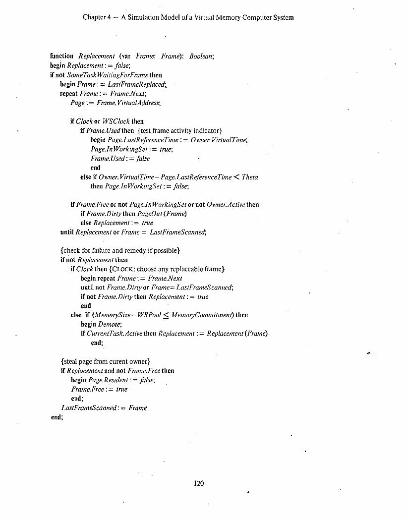
Chapter 4 - A Simulation Model of a Virtual Memory Computer System
function Replacement (var Frume: Frume): Boolean; begin Replucetnent : = fulse; if not SomeTuskWui~ingForFrume then
begin Frame : = L~ns~FrumeRepluced; repeat Frume : = Frume.Nexl;
Page : = Frume. VirlualAddress;
if Clock or WSClock then if Frame. Used then (test frame activity indicator)
begin Puge.LasrReferenceTinte : = Owner. VirlualTitne; Page. In WorkingSel : = Irue; Frume.Used : = false . end
else if Owner. VirluulTime- Page. LastReferenceTime < Theta then Page-In WorkingSel : = false;
if Frame. Free or not Puge.In WorkingSel or not Owner.Aclive then if Frume.Dirly then PugeOul (Frame) else Replacement : = [rue
until Replucemetlt or Frume = LaslFthmeScunned,
{check for failure and remedy if possible) if not Replucemettl then
if Clock then (CLOCK: choose any replaceable frame) begin repcat Frume : = Frume.Nexl until not Frutne. Dirty or Frame= Las~FrumeScanned, if not Frutne.Dirly then Replucemenl : = true end
else if (MemorySize- WSPool 5 MernoryCott~mittnenl) then begin Demole; if CurrentTusk.Acbve then Replucemen[ : = Replucemenl (Frutne)
end;
(steal page from curent owner) if Replucemenl and not Frume.Free then
begin Page. Residenr : = false; Frume.Free : = lrue end;
LustFrumeScanned : = Frame end;
120 .

Chapter 4 - A Simulation Model of a Virtual Memory Computer System
Start I Select last frame replaced I I
Select next frame
Clock / WSClock Test Use Bit
Set: (1) LR(p) + VT (2) Page in “working set”
Clear: Page not in “working set” ~~~~~~ if VT-LR(p) > THETA
L 1
4 e-
I Demote some task I
I I Choose any
/ . Yes
Queue Page for ( Cleaning
l eplace Page
\
Figure 4.7 - Replacement Algorithm
121

Chapter 4 - A Simulation Model of a Virtual Memory Computer System
Briefly, the routine uses the clock scan algorithm to search for the first clean page that is not in .v -’ .L “AZ:-*
an active-task’s working set. The essential difference between WS and CLOCK lies in (1) the
definition of “working set” and (2) the action taken when no page is .found to replace. Each page
has an associated InWorking&/ indicator which is not specific to WS, but, rather, is also used to
mark pages that CLOCK should not replace unless necessary.
Under WS, the indicator is, in effect, maintained as follows:
1) In WorkingSer is set whenever the page is referenced;
2) In WorkingSet is clcarcd whenever the page is unreferenced for more than B.
The task variable Wet-kingSetSize, which contains the number of In WorkingSet pages, is the
amount of memory committed to the task.
The implementation of the first rule is no! as straightfoward as it seems. If a referenced page is
already In WorkingSel or is not resident, no problem arises. If, however, a referenced page has
been removed from the working set, but has not been removed from the resident set and
replaced, the system will not receive an indication that the page has rcturncd to the working set
until the working set is scanned (see the next subsection). This may cause the WS load control
principle to be violated, since the amount of committed memory will be underestimated.
One solution is to remove a non-working-set page from the resident set even though it has not
been replaced; if it is referenced, a page fault will occur and the page can be reclaimed and made
both resident and In WorkingSet at the same time. The disadvantage of this method is the cost of
processing the page fault and the unnecessary mechanism to reclaim the page. See Section 2.2.5
for a general discussion of page reclamation.
In our model, WC do not attempt to analyze algorithmic overhead, and so we assume that the first
rule can be implcmcnted accurately without using a page reclamation mechanism. This is a good
example of the practical difficulties encountered in the implementation of WSEXAC~ even if the
LaslReferetzceTime register is implcmcntcd in the hardware. ,
122

Chapter 4 - A Simulation Model of a Virtual Memory Computer System
Clearing the In WorkingSef indicator is performed by the WSScan routine described below, which
is invoked independent of the replacement algorithm.
Under CLOCK, we also use In WorkingSer in a simpler mechanism that sets and clears the
indicator as part of the rcplacemcnt clock-scan. Since CLOCK load control dots not use an
estimation of the task’s working set size, the setting of In WorkingSef is irrelevant except when the
page is scanned for replacement. In this case, the frame use-bit indicates any recent references. If
the use-bit is set, then (1) In WorkingSef is set, (2) the task’s current VirfualTime is saved as the
page’s LastReferenceTime, and (3) the use-bit is cleared. In WorkingSet is cleared if the page was
not referenced since the last replacement scan and the elapsed virtual time since me
LastReferenceTime is greater than 8.
Recall, from Chapter 2, that this last criterion has a very different purpose from the similarly-
defined WS criterion. The typical CLOCK 8 is very small and is intended to ensure that an active
but I/O-bound or low priority task is given some opportunity to reference its resident pages . between successive replacement scans. The parameter is not used to distinguish active from
inactive pages.
Returning to the basic replacement algorithm for both WS and CLOCK, a page should be replaced
if it is either (1) not ZnWorkingSef or (2) owned by an inactive task. If, however, the page is
dirty, it must be cleaned before being replaced; it is queued for a writing to a slot and skipped in
the replacement scan until it is clean. Otherwise, the replacement algorithm is complete: the page
is removed. from the current owner’s resident set and the clock-scan pointer is set to start with
frame following the chosen frame.
WS and CLOCK diverge again when a complctc scan of all frames fails to find a rcplaccable
frame. To WS, this signals one of two conditions. If (almost) all frames contain active-task
working-set pages, then main memory is overcommited. This causes a task to be dcmotcd, which
should make some pages replaceable. Unless the faulting task is itself demoted, the replacement
algorithm is then invoked recursively. If, however, there arc a number of dirty-but-othcrwise-
123

Chapter 4 - A Simulation Model of a Virtual Memory Computer System
replaceable pages (the minimum number being equal to the WS free page pool size), then
memory is not overcommittcd and the faulting task must wait for a frame to be cleaned.
If CLOCK cannot find a replaceable frame in a complete scan, it simply chooses the first clean
frame ahead of the clock-scan pointer. CLOCK fails only when all frames contain dirty pages.
Working Set Scnnning
Each WS algorithm, except VMIN and WSCLOCK, performs the WSScan routine at various times
to remove non-working set pages and to calculate the task’s WorkingSefSize:
procedure WSScan; var LRUTime: fitne; begin Task. WorkingSe fSize : = 0; LR UTitne : = infinite; for Page in Task.PageTable do (scan all task Pages)
begin
.
if Page.Residenf and Page. RealAddress t Frame. Used then begin Puge. RealAddress T Frame. Used : = false; Page. LaslReferenceTime : = Task. VirlualTime; Page. In WorkingSel : = true end
else if Task. VirtualTime - Page. LastReferenceTitne 2 Theta then Page. In WorkingSe f : = false;
if Page. In WorkingSel then begin Task. WorkingSetSize : = Task. Worl+gSetSize + 1; if Page. LasrReferenceTime < LR UTime then
begin Task. LR UPage : = t Page; L,R UTime : = Page. LasfReferenceTime end
end end;
if WSFault or WSIn ferval then Task. WSScanTime : = Task. VirfualTitne + WSScanInlerval; if WSExacl then Task, WSScanTime : = LR UTime + Theta end;
124

Chapter 4 - A Simulation Model of a Virtual Memory Computer System
.- WSScun examines all task pages, including non-resident ones. If a page is resident, its use-bit is I *r
_ . LI~CGKC~; it’ It hhz F&n referenced since the last WSScan, the page’s LaslReferenceTime is
estimated to be the current VirtualTime. Any page which’ has been referenced within the last
Theta (6) references is In WorkingSet.
Under WSEXAC~, the execution model does not set the frame use-bit, but, instead, always
computes the appropriate LusrReferenceTime. With the ordinary reference string model, the
LasrReferenceTime is set correctly for every page. With the IRIM, the LusfReferenceTime is set
only for pages that arc predicted to be unreferenced for 8 or more references; for other pages the
value is “infinity”.
The scheduling of the working set scan is the fundamental difference between the WS variants.
The practical variants (WSFAULT, WSINTERVAL) schedule a scan at a fixed WSScanInlervul.
WSScun dctclmines the task’s LRUPuge, which is the In WorkingSef page which has not been
referenced for the longest time. WSEXAC~ schedules the next scan for 8 references from the
LaslReferenceTime of the LRUPuge, which is the soonest possible time a page can leave the
working set. If the IRIM is used to model WSEXAC~, the LRUPuge is certain to lcavc the
working set at that time; thus, the IRIM minimizes the number of WSScans.
VMIN attd WSCLOCK Working Set ,?Xtna/ion
The VMIN algorithm can be modeled only if the IRIM is used. Whenever the execution model
processes an idle state transition and ZRZM./enure > 8, the page is immediately removed from +
the working set. The set of In WorkingSel pages and the task’s WorkitlgSelSize are maintained
prcciscly. Thus, the lookahead VMIN algorithm is modeled simply, accurately, and more
efK?ciently than the ordinary WS algorithms.
WSCLOCK retains the essential nature of the local WS policy, while eliminating working set scans.
It calculates the task’s working set by examining each resident page in each circuit of the
replacement clock-scan. WSCLOCK uses the same criteria as CLOCK, but with 4 value of 8 that is
more suited to a WS algorithm.
125

Chapter 4 - A Simulation Model of a Virtual Memory Computer System
The primary problem with WSCLOCK occurs each time a task is activated. Since WSCLOCK
examines only resident pages, it will not remove pages that are not rcsidcnt at activation and
leave the working set after a short while. After a task has been active for 6, the resident
working-set pages will be the true working set. Thus, there is an interval following each task
activation in which WSCLOCK has no mechanism to calculate the task’s WorkingSeGize, which .
may lead to the improper activation of new tasks and overcommitment of memory.
The following solution is used in this model. When a task is deactivated, its WorkingSe6’ize is
the number of resident working-set pages; this value is used when the task is considered for a
subsequent activation. After the task is re-activated, its WorkingSetSize is the number of
remaining resident working-set pages, if any. As the task executes, it loads additional working-set
pages and the WorkingSelSize soon becomes a ‘more accurate estimate. The performance of the
WSCLOCK algorithm may be especially dependent on the use of the load control heuristic which
limits the number of loading tasks; when the loading phase has ended, the task’s WorkingSelSize
should be reasonably accurate to permit the WS load control to estimate the antount of
uncommitted memory. A more complete description of WSCLOCK and its load control may be
found in [CARRIE]. .
Loud Conbol
The remaining load control methods are’implemented as they arc described in Section 2.3. WS
load control (2.3.2) has two main parameters, Thefn (8) and WSPool (I@. CLOCK’S load control
(2.3.4) has one main parameter Co and the smoothing and confidence interval parameters, 6, a,
and tp. The LT/RT control (2.3.5) and demotion task choices (2.3.6) are also implcmcnted as
described.
126

Chapter 4 - A Simulation Model of a Virtual Memory Computer System
4.4.5 Auxiliary Memory Management
Overview
Except for the order in which page transfer requests are processed, the structure of the auxiliary
memory manager (AMM) model is highly simplified. There is no explicit representation of slots;
it is assumed that they are an unlimited resource. Only one page can be transferred in each
paging I/O operation. If multiple paging I/O devices exist, it is assumed that paging I/O
requests are balanced across the devices; the model will use any available paging device to
process a transfer request. As with the I/O device model itself, a more complex model would be
useful to study questions that are not considered here. For example, a comparison of demand
paging with either prc-paging or swapping would require modeling the concurrent transfer of
many pages in a single I/O operation. .
The interface to the AMM is through two routines: Pageln and PageOut, both of which specify a
single Frame as an argument. The Frame model contains the identity of the Page to be
transfered. The Frames are placed in a PageZOQueue according to one of three disciplines: (1)
the FIFO discipline is ordered by the time of the transfer request; (2) the Reads-First discipline
places all Pageln requests before all PageOuf requests; (3) the Running-Reads-First discipline
places Pageln requests for running tasks first, then Pageln requests for loading tasks, followed by
PageOuI requests. The distinction between running and loading tasks is described in Section
2.3.4.
,
Page Files
A page file is not a dcvicc in its own right; it is simply an indirect rcfcrcncc to an ordinary device
managed by the I/O subsystem. The page I/O scheduler makes requests to the I/O subsystem in
the same manner as tasks make I/O requests. If the model is configured to permit it, both task
and page I/O can contend for the same devices; if the Ah4M makes an I/O request on a device
that is processing task I/O requests, all requests are processed in a FIFO order.
127

Chapter 4 - A Simulation Model of a Virtual Memory Computer System
cI. -1 (5 ~WP PowFib -7 ,, rpz?rd Busy z- Boolean; Device: t Device; Frame: t Frame; . IORequest: IORequest
end;
The PageFile.Busy indicator is separate from the DeviceJusy indicator in the I/O device model.
PageFile.Busy signifies that a paging I/O transfer request is being processed on the device; a
given PageFile can make only one request at a tinie and must keep other requests pending in the
PagingIOQueue. If more than one PageFile specifies the same Device, this indirectly specifies the
number of simultaneous page I/O requests that can be queued to the Device.
Whenever a PageFile is not busy and there is an outstanding request in the PaginglOQueue, the
AMM initiates a transfer by making an I/O request. If the request is a PageOuf, the frame dirty-
bit is cleared at this time. Note that the operating system never removes a page from a task’s
resident set until that page is actually replaced. Thus, the page can be referenced and dirtied
during the PageOut transfer, setting the use- and dirty-bits once again.
The AMM processes a completed Page/n request by marking the page resident and unblocking
the task. When a PageOut completes, the AMM checks the SomeTask,WaihgForFrame
indicator; if it is set, the AMM unblocks a task which is WaifingForFrame since the PageOut
operation has (probably) made a page clean and replaceable: if there are no WaitingForFrame
tasks, the system ‘indicator is cleared. .
c..
1
128

Chapter 5
Empirical Studies
This chapter describes the use of the model presented in Chapter 4 to study policies of virtual
memory management. In Section 5.1, we describe the selection, measurement, and analysis of
sample programs. Exedution traces of these programs are processed to create reference strings
and IRIM strings. In Section 5.2, we describe the preparation of the simulation model. A
sample load is constructed using the sample programs. The IRIM is validated as an accurate and
highly efficient replacement for the reference string model.
In Section 5.3, we study the WSEXACT memory management policy. WSEXACT is tuned for best
performance over various strategies and parameter settings. We also study WSFAULT and
WSINTERVAL, the commonly-used, practical approximations to WSEXACT, and VMIN, the
unrealizabie, lookahead, version of WSEXACT. In Section 5.4, we study WSCLOCK, the ncwly-
developed WS policy.
In Section 5.5, we study the GLOBAL rcplacemcnt algorithm and load control, and tune them for
best performance over various strategies and parameter settings. In Section 5.6 we compare the
results of the three previous sections and draw conclusions about the relative performance of the
algorithms studied.
129

Chapter 5 - Empirical Studies
5.1 Task Model Preparation
51.1 Program Sample
Eight programs are selected for use in this study. These programs arc among the most commonly
used at the central computing facility of Stanford Linear Accelerator Center (SLAC). Although
computing at SLAC is heavily scientific, the sample contains mostly utility programs that are in
common use on educational and commercial systems as well. As far as we can dctetmine, none
of these programs have been explicitly written or adapted for a virtual memory environment.
Each program has a four-letter indcntification for USC in later descriptions. The programs are:
4.
LKED - IR~M 370 Linkage Editor: This program links compiler output (object modules)
and previously compiled library routines to create a load module. This program is often
the most frequently executed program on IBM 370 systems.
SORT - SYNCSORT utility program: This program is an improved version of IBM
SORT/MERGE. The program is measured while sorting some 10,000 randomly-ordered
records. A small virtual memory allocation is specified to force the program to use a
combination of internal and external sorting methods.
FORC - irIM FORTRAN H compiler: This compiler is very large and, particularly when
optimizing, slow. Most of the compiler itself is written in FORTRAN. The compiler is
measured compiling 210 statements in 2 subroutines, using the highest optimization level
(OFT = 2).
Due to its large size and a multi-phase compilation procedure, the compiler is usually
overlaid explicitly. For this study, however, the compiler is not overlaid and is executed
in a large memory allocation.
WATF - University of Waterloo FORTRAN IV compiler, WATFIV: This compiler is about
1/5th the size and 5 to 10 times as fast as the FORTRAN II compiler. It is a &bugging
130 .

Chapter 5 - Empirical Studies
compiler, which produces unoptimizcd code that makes many run-time error checks. The
program is measured compiling 1800 statements in 20 subroutines.
5. ASMC - IBM Assembler H: This program translates a 575 statcmcnt program in 370
Assembler Language.
6. SCRP - University of WatCrtOO SCRIPT text processor: This program fOmatS text,
including right-margin justification and hyphenation.
7. PASC - Stanford Pascal compiler: This program is a top-down compiler written in
Pascal. The program is measured compiling a large part (about 1100 .lines) of the
compiler itself.
8. DRAW - SLAC TOPDRAW graphics utility program: This is a FORTRAN program which is
measured while producing some of the graphs in this chapter.
Each program is executed twice, once in a normal fashion on an IBM 3701168 processor, and
once under the program execution tracer described in [sHUS78]. In the untraced mode, the entire
sample requires 10.37 seconds of CPU time. The tracing generates over 100 million bytes of trace
data (in a highly encoded format) and reveals that a total of 26,713,734 instructions are executed.
The trace data is reduced to rcfcrcnce strings, which are made as compact and as efficient to
process as possible. Since no sample program has more than 127 pages, each reference requires
one byte: 7 bits for the page number and 1 for the clean/dirty indicator. A total of 44,991,850
references are generated from the instruction traces. Table 5.1 gives statistics for each program.
A simple analysis of this data rcvcals some intcrcsting facts. Table 5.2 gives the instruction-
processing rate, memory-referencing rate, and the ratio of references to instructions for each
sample program. Programs written in higher-level languages (FORC, PASC, and DRAW) have the
highest instruction-processing rate; this is predictable, since compilers tend to generate code that
uses simpler instructions. Thcsc programs also have a higher memory-referencing rate, which is
less undcrstandablc.
131

Chapter 5 - Empirical Studies
Table 5.1 - Sample Program Data
Program Time Instructions References Pages
LKED 1.12 2,129,602 3,510,900 51
SORT 1.86 2.828.556 4,818,090 73
FORC . 1.24 4,216,349 7,218,382 124
WAT F 1.01 2,683,951 4,551,154 73
ASMC 0.97 2,276,941 3,831,515 63
SCRP 1.39 3,354,062 6,049,228 55
PASC 1.42 5,157,284 7.970.015 30
DRAW 1.36 4.066.989 7,042,566 62
Table 5.2 - Sample Program Statistics .
Program Instructions per sec.(x106)
References per sec.(x106)
References per Instruction
LKED 1.900 3.135 1.65
SORT 1.520 2.590 1.70
FORC 3.400 5.821 1.71
WATF 2.656 4.505 1.70
ASMC 2.347 3.950 1.69
SCRP 2.412 4.352 1.80
PASC 3.632 5.613 1.55
DRAW 2.990 5.178 1.73
Six of the eight programs have virtually identical references-per-instruction ratios of about 1.7.
SCRP has a higher number of references per instruction, probably due to manipulation of variable-
length text strings. PASC has a much lower number of references per instruction, probably due to
the simpler nature of compiler-gcncrated code. It is interesting that the FORTR.\N-gcneratcd code
in both FORC and DRAW has the same reference-per-instruction ratio as the assembler language
programs.
132

Chapter 5 - Empirical Studies
S&2 Lifctimc Curves
We measure the lifetime curves of the eight sample programs. Lifetime curves are not used in
the simulation model, but they serve both to ensure that our sample programs are typical and to
illustrate our earlier comment about lifetime CUIVCS. Figures 5.1(a) through 5.1(h) are the fixed-
space LRU, WS, and VMIN lifetime CUNCS of the eight programs. As expected, VMIN achieves
the highest lifetime at most memory allocations, while WS is typically, but not always, higher . than fixed-space LRU. The horizontal limit line in each figure represents a lifetime of T/m,
where T is the number of measured references and rrl is the number of distinct pages. This value
is the maximum possible lifetime since execution of the program requires a minimum of m page
faults - -
Figures 5.2(a) through 5.2(h) are long-term lifetime curves generated by ignoring the page fault
caused by the first refcrencc to each page. For refcrcnce purposes, the maximum lifetime of the
curves in Figure 5.1 is indicated on each figure. As described in Section 3.2.1, the long-run
curves are unbounded because no faults occur at the maximum memory allocation. WC also
observe that the curves have no knees. We conclude that knees are produced by measuring
programs for a limited time and including the initial page faults. If a program is.mcasured for an
indefinitely long time (assuming -that it does not terminate), the long-run behavior is knee-less.
133

2 u” C L”
I 3 1%
hp.ve 5.1(a) - LIfetIme LurveS OF LKED
_ VMIN . . . . . . . . . . .
hqure 5.lCbl - Llfetlme Curves of SQRT I , ,
I”” 1’ I, ) I , , -u I
Llmlt 6000 LRU -
ws ----. VMIN . . . . . . . . . . .
Mean Resldenc Set
I I , , , , 1
60 80
134

: Chapter 5 - Iimpirical Studies
Fqure 5.lkl - hfetlme Curves of F0RC
1' " " " " " " " " " " " " "-I
0 I I I I I I I I I I I , I I I I I lJ 0 25 50 75 100 125
Mean Resident Set
Fqure 5.1(d) - LIFetime Curves of WATF
F"""""""~""~ L
6OOOC- 6OOOC-
- - ws----. ws----.
VMIN . . . . . . . . . . . VMIN . . . . . . . . . . .
4oooc- 4oooc-
2oooc- 2oooc-
0 0 I I I I I I I I I I I I I I I I 0 0 20 20 40 40 60 60 80 80
Mean Resident Set
135

Chapter 5 - Empirical Studies
Fqure 5.1(e) - Lifetime Curves of ASMC I I I I I I I I I I I I I I I I
6OOOC-
VMIN . . . . . . . . . . .
4oooc-
Mean Resident Set
Fqure 5.1(F) - Lifetime Curves of SCRP
Limit *---a- 1 RII 1uuuuu - L””
- ws ----. ws ----.
- VMIN . . . . . . . . . . .
75000 -
25000 -
1 -’ 60
Mean Resident Set
136 ,

Chapter 5 - Empirical Studies
3
Flqure 5.1(q) - Lifetime Curves of PASC I I I I I I I I I I I I I I I I
Limit / 25OOOC& / ------- 4
0 I I I .., I I I I I 1 I I I I 0 10 20 30
Mean Resident Set
Flqure 5.1(h) - Lifetime Curves of DRAW
1ooonn t :
LRlJ ws ----.
. . . . . . . . . . . 7cnnn
: :
: . .*
. * /
’ I I I I I I I I I I 0 20 40 60
Mean Resident Set
137

Chapter 5 - Empirical Studies
Flqure 5.2(a) - Lonq-Term Lifetime Curves of LKED 150000 I 1 I I I I , I I I I I I I I
125000 - : LRU -
loooOO ~vMIN . . . . . . . . . .
I 75000 - I
Limit .’ ’
50000 -
25000 -
” ” ” ” ” ” 40 50
Mean Resident Set
Flqure 5.2(b) - Lonq-Term Lifetime Curves of S0RT 150000 I I I I I I I I I I’ I I I I I 7
; I : I
125000 - f I : LRU : I - ws --__. . . I r . I
looooo VMIN . . . . . . . . . . .
7mnn
50000 - I I I
25000 - : : ..*
. . . . . . . . . . . . * 0”-‘-’
_ -r 4 ’ I ’ ’ ’ ’
0 20 40 60 80 Mean Resident Set
138

. Chapter 5 - Empirical Studies
Flqure 5.2(c) - Long-Term Lifetime Curves of F0RC
~"""~"""'1""11""'~ I 125000 I
I I
J 100000
3
25000
A 25 50 75 100 125
Mean Resident Set
Fqure 5.2(d) - Lonq-Term Lifetime Curves of W 'ATF
125000 - 125000 - . . . . I I I I
- LRU - LRU I I
100000- ws ----' ; ; 100000- ws ----' ; ; - VMIN _ VMIN . . . . . . . . . . . ; : I 1 . .
: I : I
75000- 75000-
50000- 50000- I I I I
25000- 25000- I I I I I I I I .-
0 I I I I I I I I I I I I I I I I I I 0 20 20 40 40 60 60 80 I 80 I
Mean Resident Set I
139 ,

Chapter 5 - Empirical Studies
Figure 5.2(e) - Lonq-Term Lifetime Curves of ASMC I I I I I I I I I I I I I I- I I
125000 - I I I
- LRU I 100000- ws - - - -’ I
2 I _ z
VMIN . . . . . . . . . . . I
5 I
k 75000 - CL E Limit a E 50000 - s 2 2
25000 -
. * . . . . 0” . . ..‘L - -
0 20 40 Mean Resident Set
I I 60
Figure 5.2(fl - Long-Term Lifetime Curves of SCRP , I I I I
25OOOC- I I I I I . , 1 I I I
G :
VMIN G 150000
Limit
0 1 I I 1 I I I I I 1 0 20 40 60
Mean Resident Set
140

Chapter 5 - Empirical Studies
Figure 5.2(q) - Lonq-Term Lifetime Curves of PASC
1 LRU il
ot ’ I I I I I I 1 I I I I I ,
0 10 20 30 Mean Resident Set
Fqure 5.2(h) - Long-Term Lifetime Curves of DRAW
25000 I
AAAAA I RI I
t: VMIN .
----.
suuuu
I
: /I /- : : .*. . . **- /
/ / -’ 1 . .-* . . I,
Ohi . / Y
0 .’ . . . I 1 I I I I I I I I I
20 40 60 Mean Resident Set
1
141

Chapter 5 - Empirical Studies
5.1.3 IRIM String Preparation
Before creatkg the IRIM strings for use in the simulation model, we perform a preliminary
analysis of the relationship bctwccn w, the IRIM window size, and the amount of string reduction
compared to rcfercnce strings. Figure 5.3 illustrates this relationship for each of the eight
programs. In Figure 5.4, the curves arc combined to illustrate the similarity in the reduction
factors for most programs.
Tables 5.3 through 5.6 present detailed measuremeks of the IRIM for w= 500, 1000, 5,000, and
10,000.
Table 5.3 - IRIM Records - w = 500
Program Busy-Clean Record Type Total -Reduction Busy-Dirty Idle Records Factor
LKED 5092 3867 8850 17809 197 SORT 9392 7690 15312 32394 149 FORC 20338 15173 34384 69895 103 WATF 14349 11512 25760 51621 88 ASMC 17162 7897 24900 49959 77
SCRP 27859 13939 41504 83302 73
PASC 14057 5516 17227 36800 217 DRAW 11434 11139 22321 44894 157
Table 5.4 - IRIM Records - w = 1000
Program LKED
SORT
FORC
WATF
ASMC
SCRP
PASC
DRAW
Record Type Total Reduction Busy-Clean Busy-Dirty Idle Records Factor
4074 2983 6983 14040 250
5925 6487 11279 23691 203
11108 9357 19857 40322 179 11029 7927. 18810 37766 121
9195 4741 13807 27743 138
19623 7699 26939 54261 111 11208 5332 14240 30780 259
7721 8317 15739 31777 222
142

Chapter 5 - Empirical Studies .
Program LKED
SORT
FORC
WATF
ASMC
SCRP
PASC
DRAW
Table 5.5 - IRIM Records - w = 5000
Record Type TOtd Reduction Busy-Clean Busy-Dirty Idle Records Factor .
1846 ' 1201 3034 6081 577 3311 4937 7981 16229 297 1960 2488 4234 8682 831 ' 1170 1417 2547 5134 886 . 1753 729 2462 4944 775 5058 1547 6470 Go75 ( 463 3949 398 4347 8694 917
* 2084 2952 4888 9924 710
Program LKED
Table 5.6 - IRIM Records - w = 10,000
Record Type Total Reduction Busy-Clean Busy-Dirty Idle Records Factor
670 613 1273 2556 1374 SORT 1308 3227 4378 8913 541 FORC 744 1249 1880 3873 1864 . WATF 571 818 1379 2768 1644 ASMC 1305 478 1769 3552 1079 SCRP 2348 500 2737 5585 1083 PASC 221 206 427 854 .9333 DRAW 1018 1827 2779 5624 1252
In the simulation studies, we use IRIM strings gcncratcd with w = 5000 for two reasons. First,
this value is smaller than any WS parameter, 8, we will consider. Practical values of B usually
exceed 5000 by an order of magnitude. Second, the value of 5000 is sufficiently smaller than the .-
minimum time a program usually executes bctwcen I/O requests or quantum expirations. Thus,
the granularity of the IRIM is small compared to time-scale of events that cause task deactivations
that, in turn, lead to errors in the IRlM.
At w =5000, the IRIM reduces the trace length for all eight programs from 44,991,850 references
to 72,763 IRIM records, a factor of 618. Of course, each IRIM record is 8 bytes, so the net
volume is reduced by a factor of 77. An analysis of the reduction in simulation cost appears in
Section 5.2.
143
-_- -- --

Chapter 5 - Empirical Studies
.003* String Reduction
.04I2.
a01 .
.004’
.003~ String Reduction
a02
.ool
.004-
.003 - String Reduction
.002-
.001
! \
lked
I I I 8000 16000 24000
IRIM Parameter .004’
\ watf .OOl .
I I I tjoocI 16000 24000
IRIM Parameter _
i \
.OOl draw
L 8ooI) 16000 24000 6000 16000 24000
IRIM Parameter IRIM Parameter
.003- String Reduction
.002-
ml-
003. String Reduction
.002.
.003~ String Reduction
&JO0 16000 24000 IRIM Parameter
.003~ String Reduction
.002.
\ asmc .OOl’
I I I I I I
6000 16000 24000 8000 16000 24000 IRIM Parameter IRIM Parameter
\, fort ’
8000 16000 24000 IRIM Parameter
\
.
scrp \
Figure 5.3 -
IRIM Efficiency
144

String Reductic
Factor
Chapter 5 - Empirical Studies
--T- I I I I I 4ooo 6000 12000 16000 20000 24000
IRI Model Parameter
Figure 5.4 - Composite IRIM Efficiency
5.1.4 Task I/O Request Model
The occurrence of task I/O requests is modeled stochastically. When each of the sample
programs is traced, we obtain counts of disk I/O operations. By dividing the program execution
time (i.e., total references) by the I/O count, we determine the average execution time between
I/O requests as shown in Table 5.7. We assume that the time bctwccn I/O rcqucsts is
exponentially distributed (i.c., the requests form a Poisson process) and have a minimum value of
145

Chapter 5 - Empirical Studies
5000 rcfercnccs. This minimum value is a realistic assumption for modeling real systems, due to
the extensive processing usually required to request, verify, initiate and terminate an I/O
operation.
Table 5.7 - I/O Request Model
Program Trace Mcasurcmcnts Processing Interval Model
References I/OS Minimum Mean Distribution
LKED 3,510,900 239
SORT 4,818,090 227 FORC 7,218,382 53 WATF 4.551.154 74 ASMC 3.831.515 89
SCRP 6,049,228 56 PASC 7.970.015 325 DRAW 7,042,566 ‘31
5000 14686 Exponential ’ 5000 21233 ”
5000 136226 ” 5000 61486 ” 5000 43033 ” 5000 108035 ” 5000 24493 ” 5000 227096 ”
5.1-S Workload Model
The workload of the simulation model is specified as a set of task prototypes, one of which is
chosen to describe each newly admitted task. In the studies that follow, there are eight prototype
tasks, corresponding to the eight sample programs. A pseudo-random number gcncrator is used
to select each of the eight task prototypes with equal probability. This generator is independent
of all other random gcncrators; its seed can be specified as part of the simulation input. Thus,
the workload is easily controlled and duplicated.
Preliminary tests have demonstrated that both the distribution of prototype tasks in the workload
and the order in which they are chosen have a great effect on pcrformancc in the simulated
system. The variation due to workload differences can overshadow the variation due to any of
the algorithm and policy alternatives we seek to evaluate. If the purpose of the model were to
evaluate a computer hardware configuration for some real installation, we would have to bc very
scnsitivc to this problem. Long simulation run times and multiple replications would bb rcquircd
146

Chapter 5 - Empirical Studies
to remove effects due to variations in the load. It would also be necessary to determine whether es 4 J’. 3ur sample progrz were typical of the workload at the installation to be evaluated.
Since the object of this work is to evaluate algorithms and policies, we arc concerned with the
relative, not absolute, level of performance with any realistic, but precisely repeatable, workload.
In the studies that follow, the order in which tasks are admitted is the same in each run. The
simulation is run until the first 50 tasks are completed. Since the typical multiprogramming level
in the model system is about 5, many different groupings of the eight prototypes are processed
concurrently during each simulation run.
5.2 System Model Preparation
52.1 Model Configuration
We model a computer system which has a processor speed roughly the same as the IBM 370/168.
The basic time unit of the simulation model is a memory reference and our program sample
conveniently reveals that the 3701168 processes about 4,000,OOO references per second. The
selected configuration contains two types of I/O devices: disks, which are used for task I/O
requests, and drums, which are used for paging I/O. The service times for each device are
assumed to be uniformly distributed between the minimum and maximum values shown in Table .
5.8.
Table 5.8 - I/O Devices Model
Device Scrvicc Time (370/168) Model Parameters
Min. Max. Min. Max. Distribution
DISK 37.5 msec 57.5 msec 150000 230000 Uniform
DRUM 7.5 mscc 12.5 msec 30000 5ooofl Uniform
Although the simulator is capable of modeling contention for each disk, including the
maintenance and mcasuremcnt of request queues, the experiments in this study assume that the
147

Chapter 5 - Empirical Studies
system is disk-rich and that no queucing of task I/O requests occurs. Contention for drums, on
the other hand, often has a significant effect on virtual memory management. The model
assumes a finite number of drums (typically one) which process one paging I/O request at a time.
The remaining configuration parameter is the size of main memory. We performed a number of
simulation runs to obtain a rough estimate of the effect of main memory size on performance.
The runs used the WSEXACT replacement algorithm for a range of values of 0, and for memory
sizes of 200, 250, 300, and 350 pages. As shown in Figure 5.5, there is a roughly linear
relationship between system performance and main memory in this range. We desire a
configuration which is not abnormally constrained by memory size, but one in which a more
efficient use of main memory would result in a significant improvement. WC selected 250 page
frames for our standard memory configuration.
.7 - Frames 350
.6 - 300 Processor 250 Utilization’ 5 -
700
.4 - Replacement Algorithm: WSEXACT
.3 - Theta (xl 00,000)
I I I I I I I I l I I I I 1
5 10 20 30 Figure 5.5 - Main Memory Size vs. Utilization
5.2.2 Validating the IRIM
The task model can be driven either by ordinary rcfcrcncc strings or by IRIM strings, although
the former arc too costly for practical use. As described in Chapter 4, the model is precise except
when a IRIM busy page is removed from the resident set when rhc task is inactive. Errors can
occur when a program is deactivated and later reactivated, or when a global replacement
algorithm is forced, by ovcrcommitment, to remove a busy page.
148

Chapter 5 - Empirical Studies
In Chapter 4, we argue that the effect of such errors will bc small: in this chapter, WC present ~ 1 ‘C :. ,:: tsar. _
evidence to support that argument. We simulate our standard configuration model using both
WS and CLOCK replacement, repeating each run twice-once using ordinary reference strings and
once using IRIM strings. As indicated in the next section, rcfcrence string simulation is very
inefficient and the number of validation runs is limited by the cost.
. Figures 5.6 and 5.7 display the mean processor utilization as a function of total simulation time.
There is close agreement between the two models in each case. When a disagreement does occur, . ‘-IRIM performance is below than the reference string model. This is expected since, at each
. activation, the IRIM simulates immediate page faults on any busy pages not in the resident set;
when execution is modeled by the reference string, these faults may not occur for up to w
r,references after reactivation. Note, also, that the IRIM recovers from its underestimate of
performance since the refcrcncc string model encounters most of the same faults at a later time.
We do not claim that the IRIM will always recover from underestimation, but the empirical
results are encouraging.
Figures 5.8 and 5.9 compare system utilization for the two models in each lo-second period of
_ simulation time. These graphs show that both models have similar short-term behavior patterns.
149

Chapter 5 - Empirical Studies
150

I
: F q u r e 5 .7 - IR IM V a h d a tlo n - C lock 0 .70 -11 II~ I i l l j l l l l l IIIII III I-
0 .6 5 -
0 .6 0
0 .5 5
0 .5 0
0 .4 5
E
R e fe rence S tr lnq IR IM (5000 ) ----.
0 .4 0 1 1 ’ ’ ’ ’ ’ ’ ’ ’ ’ I ’ ’ ’ I I ’ ’ ’ ’ ’ ’ ’ ’ 1- l 0 1 0 0 2 0 0 3 0 0 4 0 0
S lmu la tlo n Tim e

Chapter 5 - Empirical Studies
I-““1 [“I
l”““I”l”“’
IIlIlIllllIllllIIlllIIlll1(-J
0 all
ul “;
c\i 0
,: d
d 0
0 d
152

Chapter 5 - Empirical Studies
/2 > - --
- -
---
153

.. Chapter S - Empirical Studies
5.2.3 Simulation Efliciency
Measurements of simulation efficiency are based on the IRIM validation runs of the previous
section. We consider raw simulation efficiency, and the relative efficiency of the reference string
and IRIM string models. It is assumed that the IBM 3701168 (used to make the simulation runs)
is nominally capable of processing 4,000,OOO references per second of processor time.
Table 5.9 shows that, with the IRIM, simulation time proceeds about 10 times as fast as real time,
while the reference string model reverses that ratio.
Table 5.9 - Simulation Efficiency
Replacement Algorithm/Model
WSEXACT/IRI(5000)
CLOCK/IRI(5000)
Simulated Time (lo6 references)
444
459
Run Tie Simulation Sim.Time/ (CPU cost (106 Sim. Cost Seconds) references) Ratio
10.68 42.72 . 10.39/l 12.16 48.64 9.4411
WSEXACT/Ref. String 271 1700. 6800. l/25.1
CLOCK/Ref. String 459 774.' 2996. 116.5
Reference String Eflciency
We claim that the simulator, as constructed, represents a “best-effort” attempt to use reference
strings as efficiently as possible. When the simulator was first written, it was presumed that
reference strings would be the primary method of driving the task model, despite the anticipated
high cost. Considerable effort was expended to minimize the cost of using reference strings
before it was realized that some other method would be necessary.
The simulator is executed under a monitoring tool which samples an executing program and
estimates the amount of processor time used in each section of the program. When reference
strings are used to drive the simulator, over 99% of processor time is used in fetching the strings
and simulating memory references. Table 5.10 differs from the previous table because it is based
on the number of successful refcrenccs simulated instead of total simulated time.
154

Chapter S - Empirical Studies
-. . P . . _ 4 Table 5.10 - Reference String Efficiency
Replacement References Run Time cost Real Reference Times/ Algorithm Simulated(@) (CPU Set) (lo6 refs) Simulated Reference
WSEXACT 163 1700. 6800. 41.7
CLOCK 274 774. 2996. 10.9
Under CLOCK, about 11 reference times are required to simulate each rcfcrence. This cost is very
low; the simulator must access the reference string record, separate the dirty indicator from the
page number, access the proper page model data structure, verify that the page is resident
(signaling a fault if it is not), access the proper frame model data structure, set the frame’s use-bit,
test the dirty-reference indicator and possibly set the frame’s dirty bit, update the task’s virtual
time, check for a simulated interrupt event, and, finally, move to the next reference record while
checking for an end-of-buffer condition. Although some techniques were used to perform several
of the above operations simultaneously, it is estimated that about 20 to 25 memory rcferenccs are
required.
To explain this discrepancy, WC postulate that an unusually large proportion of memory refcrcnces
were to the 3701168 cache memory, making the effective memory reference rate much greater
than 4,000,OOO per second. The .rcferencc simulation loop is small and executed many times in
succession so all instructions should occupy the cache almost all the time. The linear access of
the reference string, one byte for each refercncc, implies that a non-cache memory access is
required a small fraction of the time. Most references can bc simulated without updating any *.
memory location (e.g., it is not necessary to set a use-bit which is aheady set). Since the IBM
architecture uses store-through cache policy, store references have a higher average cost than fetch
rcfcrcnces; thus, average programs that have a reasonable proportion of stores will achieve a
lower references-per-second rate than a program that stores infrequently.
Although we are not prepared to suggest a practical alternative, this discrepancy is a good
example of one of the weaknesses of the reference string model. Many circumstances can cause
references to require widely varying amounts of time to bc processed. ’
155

Chapter S - Empirical Studies
Shnutation of WSExAcr, using reference strings, is considerably more expensive than the other
algorithms, including the other WS algorithms. The WSEXA~ algorithm must update a table
containing the page LastReferenceTime, requiring at least one store access per simulated reference
and a slower memory-referencing rate.
IR IM String Fficiency
When the simulator was monitored when processing IRIM strings, approximately 40 to SO% of
processor time is consumed simulating memory references. In Table 5.11 we assume the SO%
figure in estimating the cost of reference SiIIIUkitiOn.
Table 5.11 - IRIM String Efficiency
Replacement References Algorithm Simulated(106)
Run Time (CPU Set)
cost Simulated References/ (lo6 refs) Real Reference Time
WSEXACT 273 10.66 21.36 12.7 CLOCK 274 12.16 24.32 11.2 -
The efficiency of IRIM itself (i.e., separated from the full simulation model) is about 10 simulated
references per real reference time, with only a small penalty for simulating the WSEXACX
replacement. Compared to using rcfcrcnce strings, IRIM strings are about 100 times as efficient
for practical replacement algorithms and about SO0 times as efficient for WSEXAC~.
5.3 Tuning the WSEXA(JT Replacement Algorithm
The following sections describe a number of experiments to measure the effect of various
parameters and policies on a system with the WSExi\c~r replacement algorithm. Our dual
purpose is to understand the nature and cxtcnt of each effect and to tune the WSEXNX for best
performance before it is compared to global replacement E&h experiment consists of simulating
the system with the standard configuration and workload described in the previous section. For
each set of parameters to be tested, the system is simulated for a range of values of the working
156

Chapter 5 - Empirical Studies
.set parameter, 6. The resulting performance measures are plotted, producing a curve such as the
one in Figure 5.10.
Figure 5.10 - Sample WSEXACT Performance Curve 0.70 I 1 I , I I I I I I I I , I I I I
0.65 I
0.4ot 1 ’ ’ ’ ’ ’ ’ ’ ’ ’ ’ ’ ’ ’ ’ ’ ’ ’ ’ ’ ’ ’ -I
0 500 1000 1500 2000 WS Parameter - Theta (x 1000)
In preliminary tests, we have found that the value of 0 that optimizes performance will vary
considerably from one set of parameters to another. Furthermore, since real workloads vary
considerably, it is not practical to determine the optimum value of B for a sample workload and
expect it to be optimum for the entire workload. Thus, it is necessary to consider the sensitivity
of performance to 8.
,
An example of the problem we try to avoid appears in Figure 5.11. In Example 1, the two curves
are practically the same, except for one point at peak performance. A simple comparison of peak
performance would lead us to an unjustified conclusion that one model is better than the other.
Another effect that we wish to examine is the stability or robustness of a particular model. In
Example 2, both models have the same peak performance but model A is preferable to model B.
157

Chapter 5 - Empirical Studies
Processor Jtilization
Models A B ---.
Tuning Parameter Tuning Parameter
Processor Utilization
Models A B
---
I / \ / \ / Example 2 \
Figure 5.11 - Comparing Models
53.1 Task Demotion Policy
We consider the six task demotion policies described in Section 2.3.6. As shown in Figure 5.12,
there is little significant difference between choosing (1) the most recently activated task, (2) the
task with the smallest resident set, or (3) the task with the largest remaining quantum. This is not
surprising, since each of these policies will often result in demoting the same task: the most
recently activated task is also the one that has had the least opportunity to load a large resident
set or consume its quantum.
Somewhat less effective is the policy of demoting the faulting task. Apparently, the elimination
of a single replacement and paging-I/O operation for each demotion does not result in a
significant saving. This policy is still better than random selection, probably because the last
activated task (or smallest task) also has a greater chance of faulting. Demoting the task with the
largest resident set is a worse policy than random choice.
In Figure 5.13, WC examine the relationship bctwccn the demotion policy and the frequency of
overcommitment and demotion. Surprisingly, the three superior policies have significantly more
demotions (60 to 80% more in the peak performance range) than the poorer policies. Apparently,
the tasks demoted by these policies are considerably smaller than the average task, indicating that,
overcommitment must occur shortly after a task is. newly activated and before it has had a chance
to gather a large rcsidcnt set.
158

Chapter 5 - Empirical Studies
Figure 5.12 - Demotion Task Choice vs. Utlllzatlon - WSEXACT 0.62 I I I 1 I I I I I I I I I I I I
g -c: -.-._,
0.60 - ,.,/~./ ..-.*i...-y \.,...............,~~
‘“-c ‘. . .
0.58
0.56
----_ \I .I .Y”l I
LONGEST --’ . . . . . . . . . . . . . . . . .
LARGEST - - - - - - SMALLEST -__---- k;JTACRTIV -.-.-.-.-.- I 0 I I I I I I I I
500 1000 WS Parameter - Theta (x 1000)
Flqure 5.13 - Demotion Task Choice vs. Demotions - WSEXACT
80
60
--- (,-~~~/-~--.~
-. -----+I
20 FM””
L-
$i F, n
m$
--_-- . . . . . . . . . . . . . . . . .
- - - - --
MALLEST ------- ;iLTA”R”V -.-.-‘-.-.-
1 I I I1 I I, I1 1 500 1000 1500 2000
WS Parameter - Theta (x 1000)
J
159

.’ Chapter 5 - Empirical Studies
c
5.3.2 LT/RT Co&i a --- --_ -. -
e‘ _ 1. j -.Lw mdy.
The LT/RT nechanism to limit the number of loading tasks is described in Section 2.3.2. The
control has two tuning parameters: (1) a newly activated task is considered to be a loading task
until it has cxccuted T references or has made an I/O request; (2) the system never activates a
task if there are L loading tasks in the active queue.
Figure 5.14’ shows system performance with various values of L with the standard model
configuration of one paging device. Performance degrades with increasing L, supporting the
hypothesis that the number of loading tasks should not exceed the number of page faults that can
be serviced simultaneously. In Figure 5.15 a model configuration with two paging devices is
mcasurcd; the resulting performance curves for L=l and L=2 are comparable, and both are
better than larger values of L.
Figure 5.14 - Loadrnq Task Llmlt - WSEXACT I 1 I I I I 1 I I 8 I I I I I I
0.625 - I ,
--I
_-----_ I’
-s ONE PAGING DEVICE -.
,I *. -.
nl5ni-l -..,-- t
1
,I’ I’
,.... . . . . . . . . ‘.~~~;:: ‘-.--- _-__ : ‘. --._
I :. : . . I . . :. . . --s_
. . : z , : .:’ / \ / -w -.-.. . . . . . . . . . . . . . . . . . . .
0.575
0.525
t ; / ,’ “/;r\*,/-\~‘-------
’ I lJ -.-.-.-.-.- 0.500 ‘I: d I I I I L I I I I I ,
0 500 1000 1500 2000 WS Parameter - Theta (x 1000)
160

Chapter 5 - Empirical Studies
Fqure 5.15 - Loadlnq Task Limit - WSEXACT 0.72 I I I I I I I , I I I I I I I I I
TW0 PAGING DEVICES
0.70
0.68
0.66
0 .64 k!jr
,/‘\\,\ - - e-,x,, . . . . . .I
I E .‘I/ Task Limit ‘\ / .\
I ./. \ -=\ \
500 1000 1500 2000 WS Parameter - Theta (x 10001
Flqure 5.16 - Loadlnq Task Lifetime- WSEXACT 0.62 a , , r , , , I I , I I I I I I I 1 I 1 , I I
0.60
0.58
0.56
Llfetime
250 500 750 1000 1250 1500 WS Parameter - Theta (x 1000)
*
161 .

Chapter 5 - Empirical Studies
Figure 5.16 shows the effect of T. The six performance curves are rcprescntative of a much larger
number of tested values. As T is increased to 15000, there is a steady, logarithmic improvement
in performance. Alter this point, performance declines very slowly. These results demonstrate
the robustness of the contol mechanism if T is larger than the optimum. If T is too small, some
programs will be faulting frequently when the system no longer considers them to be loading
their working sets; this error should be avoided.
5.3.3 Paging Queue Order
Figure 5.17 shows the performance of the mode1 system under three paging I/O qucueing
policies: (1) page-ins and page-outs are processed in the order rcccived; (2) all page-ins are
processed before page-outs; and (3) page-ins for running programs are processed before page-ins
for loading programs, which are processed before page-outs. The effect of processing pagc-in I/O
operations before page-outs is clear.
Flqure 5.17 - Paqlnq Queue Order - WSEXACT
0.65t’ ' ' '
0.60
0.50 p#s;AULTS
READS FIRST--------
FIF0 -----
0.451"' ’ ’ ’ ’ ’ ’ ’ ’ ’ ’ ’ ’ ’ ’ ’ ’ ’ ’ ’ ’ J 0 500 1000 1500 2000
WS Parameter - Theta (x 1000)
162

Chapter 5 - Empirical Studies
5.3.4 WS Free Page Pool Size
The effect of varying the WS free page pool size Ko is unclear, but we can still tune WSExAct’
satisfactorily. We measure the model system for values of Ko between 0 and 25, in steps of 5,
(Figure 5.18(a)) and between 0 and 125 in steps of 25 (Figure 5.18(b)). While the best
performance results for Ko=O, the amount of degradation when KO is 5, 10, 15, and 20 follows no
obvious pattern. The range of performance between Ko=O and Ko=25 is small: the maximum
difference is approximately .7%. For larger values of Ko, there is a clear decline in performance
as the pool size increases.
The purpose of the free page pool is to reduce the frcqucncy of memory overcommitment and
task demotion. It also has a negative effect of depressing the multiprogramming level and, thus,
processor utilization. In Figures 5.19(a) and (b), KO has the expected effect on the number of
demotions. It 1s interesting that the number of demotions is approximately constant across the
range of 6’; the significance of this observation is unclear.
In the next pair of Figures, 5.20(a) and (b), the effect of Ko on the multiprogramming level is
shown. Here we see little discernible difference when Ko is 5, 10, or 15, which corresponds to the
anomalous performance effect. As Ko is increased, the positive effect of reducing
overcommitment and demotions dominates the negative effect of reducing the multiprogramming
level. In general, the need for a free page pool is questionable.
163

Chapter 5 - Empirical Studies
I Figure 5.18(a) - Free Paqe Pool Size - WSEXACT
P ‘1 “‘I I”1 1 ,’ 0 11 ,’ I I I ,’ III
0.610
0.605
/
'. ’ 0.600 Pool Size 58
\ ’ -------we_. . 1 \ \ . . . . . . . . . . . . . . . . . '. \
ip -- . . \ \ ----.
--me__- '. 1, -.-.-.-.-.- . . 1,
0.595[' " "I FL ' " ' " 1 -\
I"; 1 " 1' 400 600 800 1000 1200’
WS Parameter - Theta (x 10001
Flqure 5.18(b) - Free Paqe Pool Size - WSEXACT
0.600
6 c t-i
0.550 =i d 2
0.525 -. I -. Pool Size i$g ------- ---, *. -. . . . . . . . . . . . . . . . . . -. 0.500 gg -- ----.
--_---- -.-.-.-.-.-
tIIIII~rJI~~~i~~~~I~~lIIIIIl 400 600 800 1000 1200
WS Parameter - Theta (x 1000)
f
164

Chapter 5 - Empirical Studies
-- . Flqkre 5.19(a) - Paqe Pool vs. Demotions - WSEXACT
~‘l”“I”“I”“I”“l”‘~
____-------_ ----
--__ ---_
---.--
--_---- ---a -v-r<
._,.,........‘.‘.
“.“‘.““..........,_,...,,,,....’ ,.......- --mm ---_______-____-_-_------------
c--
1 Pool Size $8
---- ---_--. . . . . . . . . . . . . . . .._
20
! ------ -__-__- -.-.-.-.-.-
tIIIIIIP,I,,i,,,,l,,,,l,,,, 400 600 800 1000 1200
WS Parameter - Theta (x 10001
Fqure 5.19(b) - Page Pool vs. Demotions - WSEXACT
80
60
-- -----.__ ________ ------u_-_
-_-____-w-c- ---_ _---
--- . . . . . . . ,.,....................
.~;.....................‘.“‘” ----_ -___r_-_----- ---___________or--
Pool Size 125 ----------.
% . . . . . . . . . . . . . . . . ----_-.
-20 -_--__- -.-.-.-.-.-
400 600 800 1000 1200 WS Parameter - Theta (x 10001
165

Chapter 5 - Empirical Studies
Flqure 5.20(a) - Paqe Pool vs. MPL - WSEXACT
I:ll,,,,P,,,,i,,,,l,,,,l,,,l 400 600 800 1000 1200
WS Parameter - Theta (x 10001
Flqure 5.20(b) - Paqe Pool vs. MPL - WSEXACT’
5.5
4.0 F
‘.* -.-,
-.-,
--\ --Zs
---_ --A.-- --
-- ---z
--+ --
-- -‘A
--__ “W.
.‘......,, -- . . . . . .
. . . . . . . . . ---_
--
. . . . . . . .
‘.. . . . . . . . . . . . . . . . . . . . . . . . .
---_ --
1 --S_ --__ ----_
-_----_ 3.0 - -.-.-.-.-.-
, 1 I I 1 I I I I I I I I I I I I I , I, 400 600 800 1000 1200
WS Parameter - Theta Cx 10001
166

Chapter 5 - Empirical Studies
53.5 Evaluation of WS Approximations and VlU$ ~ - .o*.
The practical WS approximations, WSFAULT and WSINTERVAL, are measured using the same
configuration and load. The tuning parameters determined in the previous section are set to the
values that optimized the performance of WSEXACT; although it is possible that different values
would optimize each of the approximations, our experience with tuning WSEXACT indicates that
the improvements would be minimal.
In Figure 5.21, WSEXAC~, WSFALTLT And WSINTERVAL, achieve about the same peak
performance. Although the practical algorithms appear to be more sensitive to 8, the maximum
observed difference among the algorithms is about 1.5%.
Finally, Figure 5.22 shows that the lookahead algorithm VMIN is considerably better than
WsEx~cr. ‘I’hc maximum difference in processor utilization is 6%, which represents a
throughput improvement of 10%.
Flqure 5.21 - WSEXACT, WS--FAULT, W-S-INTERVAL 0.650c I n I I , I I I I , I 1 1 1 1 1 1 1 1 1 14
0.625 -
0.550 4 -'I - I
0.525 f WSEXACT
WS-FAULT -------- -1
I WS-INTERVAL- - - - -
0.500 I I I I I I I I I I I I I I I I I 0 500 1000 1500 2000
WS Parameter - Theta (x 1000)
167

Chapter 5 - Empirical Studies
Flqure 5.22 - WSEXACT, VMIN
----c 1 WSEXACT VMIN --- -----
““““J”““““‘_ 0 500 1000 1500 2000
WS Parameter - Theta (x 1000) _ _--.,-
5.4 Tuning the WSCLOcK Replacement Algorithm
We have verified that the the demotion-task policy, the LT/RT control, the paging queue policy
and the WS free pool have the same effect in WSCIDCK as WSEXAC~. Since the LT/RT control
is a basic element of WSCLOCK, its effect is shown in Figures 5.23 and 5.24.
168

Chapter 5 - Empirical Studies
Flqure 5.23 - Loadlnq Task Limit - WSCL0CK
0.625 0NE PAGING DEVICE
*. -*.- -s
: .‘.‘...., ----we_* ‘. . . . . . . : . . . -. . ...’ . . . . . . . . . . . . . -. . . . . . -. *. . . . . /./\ . . --.
L; :I 1 ‘. . 0.550
0.525 ----.
-__-___
0.60
0.58’ Lifetime
‘58888 ----------. . . . . . . . . . . . . . . . . .
15000 - - - - - - 1 wt ----_-- -.-.-.-.-.- 0.56 I”” ’ ” ’ ’ ’ ’ ’ ’ ’ ’ ’ ’
1po I I 1 I I I I I I I 250 500 750 1000 1250 1500
WS Parameter - Theta (x 10001
169

Chapter 5 - Empirical Studies
5.5 Tuning the CLOCK Replacement Algorithm
The procedures of this section follow those of Section 5.3, except that the performance of CLOCK
is observed over a range of the control parameter CO.
5.51 Task Demotion
Measurements of the six task demotion policies under CLOCK confirm the observations made
under WSEXACI‘ (Figure 5.25). Demoting (1) the task with the smallest resident set, (2) the task
with the longest remaining quantum, or (3) the last activated task all result in comparable
performance. Demoting the faulting task is poorer that these three but better than random
Demoting the task with the largest resident set is worse than a random selection.
Figure 5.25 - bemotldn T.ask Choice- CL0CK 0.650 , a , , I I I I I I I I I I I I a I I I I I,
0.625 -
0.600 -
0.575 -
0.550 -
0.525 - RANDBM --_--
idEf . . . . . . . . . . . . . . . .
SMALLEST - - ----.
-----_- k;;TT$TIV -‘-.-.-.-.- I I I I I 1 8 I I I I I(
0 0.2 0.4 0.6 0.8 1 Clock Control Parameter
P.
170

Chapter 5 - Empirical Studies
5.52 LT/RT Control
Measurement of the LT/RTcontrol shows it to bc useful under CLOCK (Figure 5.26) but having
a somewhat different effect than under WSEXACT (see Figure 5.14). Under WSEXACT a loading-
task limit L=l is significantly superior to L>l, while under CLOCK both L=l and L=2 are
similar and are significantly better than L>2.
A clue to explaining this unpredicted result is the behavior to the right of the peak performance,
where L= 1 is superior to L=2. In this range of CO, the multiprogramming level is higher than
optimal and, thus, there is more opportunity for more than one loading task to bc activated at the
same time. We surmise that, at near-peak performance, the CLOCK load control naturally limits
the number of loading tasks to po more than 1 and, in cases where two loading tasks are
activated, competition between them has no ill effects.
Flqure 5.26 - Loading Task Limit - CL0CK
0 0.2 0.4 0.6 0.8 1 Clock Control Parameter
171

Chapter 5 - Empirical Studies
The effect of the loading-task lifetime 7 is quite small in the peak-performance range and grows
in importance as CO, and the multiprogramming level, become higher than optimal (Figure 5.27).
As shown in Figure 5.28, larger values of T depress the multiprogramming level and
counterbalance a larger-than-optimal CO, increasing the robustness of CLOCK.
We choose L= 1 and T= 15000 as our tuned system parameters; these represent a favorable
compromise between peak performance and robustness.
Flqure 5.27 - Loading Task Lifetime- CL0CK 0.62 I,, , , , , t r I I I I I I I I I # I I I I
0.60
0.58
0.56
0.52 0 0.2 0.4 0.6 0.8 1
Clock Control Parameter
172

Chapter 5 - Empirical Studies
5.25
-_--. I Flqure 5.28 - Loadlnq Task Lifetime vs. MPL - CL0CK
LIFetime 100000 --- ----- --. gf-J(-J; ------. . . . . .
I I I 0.6 0.8 1
Clock Control Parameter
173

Chapter 5 - Empirical Studies
5.53 Paging I/O Qucuc Order
As observed under WSEXACT, ordering the paging I/O queue to process page-ins before p;ge-
outs improves CLOCK performance significantly, while ordering page-ins for running programs
before page-ins for loading programs results in only a minor improvement in peak performance
(Figure 5.29). Both of these politics, however, contribute to the robustness of CLOCK. With a
FIFO paging I!0 queue, peak ~pcrformancc is observed for a narrow range of the control
parameter CO, while the page-ins-first policy has a wider range and the running-task-page-ins-first
policy has an even wider peak-performance range.
Flqure 5.29 - Paqmq Queue 0rder - CL0CK
nc “‘“F -.-----___c . . . . \
READS FIRST------- ’ w - _ --__
--------_ 1 FIFpl _ _ _ _ _ - - -
0.0 ” ” ” ” ” ” ” ” ” ” ’ “‘I’ 0 0.2 0.4 0.6 0.8 1
Clock Control Parameter
174

: Chapter 5 - Empirical Studies
5.5.4 Cl- Load Control Parameters . L * -,.-a#
Our final tuning experiment is to measure the effect of the three CLOCK load control parameters
6, a. and ‘p. We perform a preliminary search for the optimal paramctcrs using a coarse 3X3X3
design. For each parameter, we select 3 widely-spaced values as shown in Table 5.12.
Table 5.12 - Coarse Search-Design Parameters
Parameter Values
6 (observation interval) .2 sec. .5 sec. .8 sec.
(IL (smoothing weight) .2 .5 .8
cp (confidence level) .67 .90 .98
As with the previous tuning experiments, each of the 27 parameter combinations is examined at
each of the 11 values of CO. Each simulation run models about 500 seconds of simulated time;
this single experiment represents about 40 hours of simulated time.* The results of this
experiment are not shown graphically because it is difficult to display all 27 performance curves
in meaningful combinations without overwhelming the reader.
In Table 5.13, we show the peak performance utilization observed with each parameter
combination. The diffcrencc between the highest and lowest values is only l%, and any simple
relationship between the parameters and performance is indistinct.
Table 5.13 - Peak Performance - Coarse Search Design
6 .67 .90 .98 20 .6091 .6101 .6063
ff=.2 50 .6071 .6142 .6137 80 .6114 .6102 .6148 20 .6151 .6117 .6173
a=.5 50 .6151 .6153 .6130 80 .6134 .6116 .6100 20 .6107 .6168 -6141
a=.8 50 .6136 .6098 .6158 80 .6139 .6155 .6129
175

Chapter 5 - Empirical Studies
In order to detect any subtle patterns in these results, we construct Tables 5.14-5.16. In Table
5.14, we enter the value of a which gave the best performance for each combination of the other
two paramctcrs. If performance differed by less than .l%, we entered both or all values of a.
We can see that a = .5 has a majority, but no relationship to the other parameters is evident
Table 5.14 - Peak Performance 0~‘s
Q, s .67 ..90 .98 .2 set .5 .8 .5
.5 set .5 .2, .5 .8
.8 set .5, .8 .8 .2
Table 5.15 analyzes S in a similar fashion: the value 6 = .5 has a majority; 6 has no distinct
relationship to the other parameters.
Table 5.15 - Peak Performance 6’s
v a .67 .90 .98 .2 .8’ .5 .5, .8
.5 .2, .5 .5 .2
.8 .5, .8 .2. .8 .5
Table 5.16 analyzes ry in a similar fashion: no value of ‘p has a clear majority; no relationship to
the other parameters is evident.
Table 5.16 - Peak Performance ‘p’s
a 6 .2 .5 .8
.2 set .67 . .90 .98 .90
.5 set .90. .98 .67 .90 .98
.8 set .98 .67 .90
176

Chapter 5 - Empirical Studies
Normally, WC would proceed from searching with this coarse design to searching with a refined
design in the regions of higher performance. The results of this experiment give us little
motivation to do so. The lack of any distinct difference or trend in each of the three parameters
makes it highly unlikely that there exist parameters that are significantly better.
The preceding results might lead one to suspect that the clock load control is ineffective. This is
not the case. In each of the experiments above, there are numerous (typically 50 to 100) times
that the load control detects overcommitment and demotes a task. However, it appears that the
LT/RT control plays a large part in preventing extreme overcommitment in the first place.
To show this effect, we measure the system with the CLOCK rcplaccment algorithm but without
an adaptive load control. Instead, we substituted a fixed multiprogramming-level (MPL) limit
and the Z,T/RT control. We ran the model for MPL values from 2 to 10 (Figure 5.30) and
found that performance leveled off at about 10% below the peak for MPL greater than 8.
Without the L,T/RT control, thrashing and very low performance would have resulted from
increasing MPL. Figure 5.31 shows the mean number of active tasks for each value of MPL. At
any given time the number of active tasks is limited by both the MPL limit and the LT/RT
control. At large values of the .MPL limit, the LT/RT control plays a more active role and
effectively prevents extreme overcommitment.
177

Chapter 5 - Empirical Studies
0.6 -
E 0.5 - s iz =I .-I 2
0.4 -
Flqure 5.30 - Fixed MPL Load Control - CL0CK w * c or -,‘-p “g , , I I & I I I I I I I I I I
I 1 1 I I I I I I I I I I I I I I 1
2 4 6 8 10 Multlproqrammlnq Level
Figure 5.31 - Fixed MPL VS. Mean Multiproqrammlnq Level I I I # I I I I I I I I 1 8 I I I I
6-
5-
4-
3-
2-
* I I I I I I I I I I I I I I I _/ 2 4 6 8 10
Fixed MPL Limit
178

Chapter 5 - Empirical Studies
c ’ ~-----km~~f M&EXACT, WSCLOCK, and CLOCK Policies -- .
56.1 Performance Comparison
~ The performance curves of the untuned and the fully-tuned WSEXMX, WSCLOCK, and CLOCK
policies appear in Figure 5.32. The untuned politics have a random demotion-task policy, no
LT/RT control, and a FIFO paging queue. Since the algorithms have different control
parameters, we do not compare these performance curves directly. All three policies show
sufficient robustness. Although CLOCK appears to have more sensitivity to its control parameter
Co, it has a wide range of stablility; a more “judicious” choice of parameter range (e.g., only
those between .2 and .6) would have resulted in a performance curve that has a flatter
appearance. In Figure 5.33, we show that all three policies reach their peak performance at the
same mean multiprogramming level, even though their replacement stratcgics and load controls
are significantly different.
f
179

Chapter 5 - Empirical Studies
Flqure 5.32 - WSEXACT. WSCLBCK. and CLBCK
Ir~'sI~s-'I'~'~-
*---- _---_____------___ I-
0.4 - ,I . I . I - I Tuned _ I “nruned _ _ _ - - - - -
0.2 -!
WSEXACT
oo~--zk-k4oo * 0 US Parameter - Theta Ix 10001
,\-,-* -._- --------______--_ 6 0.4 -,
z -I N :: Tuned 5 ““t”ne,j - - - - - - - - _
0.2 -
WSCLBCK
0.0 ” ” ” ” ‘I”. ” - ’ ” 0 500 1000 1500 2000 US Parmeter - That8 lx 1OOOl
0.6 ---L
, - -\ -1
\ t :,\ \ Tuned ’ \ Untuned - - - - - - - -.
\ \
t
. .
CLBCK “---- ----_---__
.

: Chapter 5 Empirical Studies Chapter 5 - Empirical Studies -
Figure 5.33 - Utlllzatlon vs Mean Multlproqrammlnq Level Figure 5.33 - Utlhzatlon vs Mean Multlproqrammlnq Level 0.65 0 I,,, 1 r l 1 r 1 r I t a I I I I I I 8 I I I I I 0.65 0 1 r 1 r 1 r t a I I I I I I I,,, , , I, 8, I I
0.60 0.60 - -
/ / 0.55 0.55 - , - ,
,I ,I /I /I
0.50 0.50 - /' - /' I' I' (.----VW- (.----VW-
,/ ,/
' ' 0.45 0.45 - I/' - I/' I' I'
I' I'
0.40 0.40 - /' - /' - I' - I' I' I'
CL0CK----------. CL0CK----------.
0.35 0.35 """""""""""'lt' """""""""""'lt' 3 4 5 6 7 3 4 5 6 7 8 8
Mean Multlproqramminq Level
Although we dislike characterizing algorithms by their peak performance, we have little
alternative. Table 5.17 gives the statistics for the peak performance observed for WSEXACT, WSCLOCK, and CLOCK for the same configuration, load, and simulation run length.
Table 5.17 - Peak Performance - WSEXACT, WSCLOCK, CLOCK
Algorithm Utilization Mean MPL Parameter
WSExAcr .6211 5.25 0=600,000
WSCLOCK .6164 5.01 e = 700,000
CLOCK .6177 5.27 co = .40
The maximum difference in performance is .47%. Considering the accuracy of the model and
non-exhaustive methods of tuning each algorithm, WC find this diffcrcncc to be insignificant.
181

Chapter 5 - Empirical Studies
_. . I We experiment with the algorithms using the tuning parameters that produced peak performance ,,. -Q. by running the simulation for a much longer time. Figure 5.34(a) shows cumulative utilization at
each point in the simulation run time. This graph, in which the utilization scale is based at zero,
illustrates the insignificance of the difference among the algorithms. In Figure 5.34(b), the scale
is reduced to magnify the difference. It can be readily seen that the load-produced variations
dwarf the measured differences between the algorithms.
In these experiments, utilization was measured for each five-second interval of simulated time.
We compare the distributions of these intervals in Figure 5.35. This figure shows that the three
algorithms have an equivalent distribution of high-utilization intervals, but that in low-utilization
intervals, CLOCK is slightly worse than the WS algorithms. A follow-up study might determine
whether the distributional difference was due to longer periods of undercommitment or
overcommitment, and determine if the load control could be improved.
Flqure 5.34(a) - Cumulative Utilization '--trov
0.6
WSEXAC- WcJ-L0C#. . . . . . . .
CL@CK-------em-.
<
I 1 1 0 I I I I I 6 I I I I I I I I I I I I I
250 500 750 1000 1250 Slmulatlon Time
182

Chapter 5 - Empirical Studies
Fqure 5.34(b) - Cumulative Utilization n7nr I , , I 8 I I I I 1 I I I I I I I I I I I I 1 i. *.)i
‘f ::.
.._ 1. WSEXACV Wg-L0C#. . .
,-Lf,CK----------.
” ” ” ” ” ” ” ” ” ” ” ‘I”’ 0 250 500 750 1000 1250
Slmulatlon Time
Flqure 5.35 - Cumulative Dlstrlbutlon OF Utlllzatlon l ‘*
0.8 - :
_ WCJ-j,CK . . . . . . . . . . . . . . . . . . . . . . . / ,r 2 0.6 ------------- ;" z if a" 0.4 0.4 -
0.2 0.4 0.6 0.8 1 Utilization in 5 Second Interval
183

Chapter 5 - Empirical Studies
5.6.2 Operating System Overhead Comparison c ** i.:- ?-San.
This research has been inspired by certain conjccturcs about different memory management
policies. [DENN80, SIM079] These conjectures hold that one policy is inherently superior to
another, without regard for the cost of implcmcntation or overhead. Thus, this work has
examined the relative performance of these policies in a model that did not include operating
system overhead.
Although the incorporation of operating system overhead in the simulation model would have
presented little difticulty, this was not done. If the model included overhead, it would have been
necessary to assign costs to each of the operating system functions. In real systems these costs can
vary considerably, depending upon the processor, the system implementation, the complexity of
the scheduler or the memory hiearchy, and the availability of special aids such as microcode space
for implementing operating system functions in firmware.
In lieu of modcling the effect of overhead, we shall present some external measures of the cost of
computing the policies studied above. This measurement dcpcnds on two factors:
1) The simulator program is written in a systems implementation language, and the
programming used to model the operating system is very close to the programming that might
appear in a real operating system. Thus the execution of the simulator program models the
execution of the model operating system.
2) There exists a method for measuring the execution of the simulator and estimating the
total time spent in each of the functional areas of the operating system model.
WC have describe the programming of the operating system model in Chapter 4. The
measurement of the simulator is performed by a program PROGLOOK described in [JOHNNY].
PROGLOOK monitors the execution of any other program and samples the program counter at
regular intervals. A histogram, such as the one in Figure 5.36, tabulates these samples and
provides an accurate estimate of the time spent in each small section of the program. With the.
184

Plll,I"O PPOPIll FOP SlTITI 1 0.911 . ..r**...*S~~.C*.*r~**.*******~
0 Pxacxlr 1 PEPCEIZ 2 PEPCXlT 3 PxlCXIT 4 PImzxIT
( 01 ( 14) ( 281 I 62) ( 56)
5Eo oKi ______________I______________I____-_-_ ------------- ------- ---a------ ,O#Bll
.**~*t.****t*t~*~~t~**I*1~~.*~*.~*..*****.L”***.***.~****..*~***4*+ . 32 537680 009680 .*t*t*~+*.*tt*t~L.**.*~*t~**‘**~*.*.********~~****.**~*****~***”...+*..+..+*t’ Trace I/O .*****.*t : 5176ao 004680 l ************ . 5,ajoo 00$.300 l tt****t*.t*t*U*.*+* . . --A- . 518310 005310 l ********** . . Disp3tcher 5 53.3910 0059,o *****t**.*t*t*t** . 53a920 005920 l ********* . -- 53aA70 005170 l *.*~**~L.**~*tt*t******~***~*~******~
-2-4
538180 005ABO l ***t*t~**~*******~t***************~***** . . 19
538190 005190 +***~****Cf*~**.ft*.****** . 12 53*AaO 005ABO ***i*~***tLt**f*t*t.t*****,***tt~ttt.t*t*t**P~tl**t*.**t*t.~t*.*+tt.**t*t**~*ttl**t**t*..*L*t . . . 5381CO 005ACO l **~~*.L******U********.***~*~.*~**~.***~*~.**~* . . 24 539,DO OcJ5~00 *.t*****~******ftt**********~****~*********~~***************.*.***..***~~**.*~***~*~***~**.******* 56 5381ZO 0051EO **t***f*t**t~tUtt~tt*********~**~******~***~***** 513800 005830 l *tt.**~***tt*****t****~***~~***********~* . :i 538810 005810 **t***.~*~**lt~****.~~***...~~~*****~~.~.*~~*~*.~~~*****~***~~ . 29 533890 005890 l ~tt***~****lf”***t~***.******~*~*~ . . . 17 538310 005810 .***********t****f***************~~***~ . . 18 5388CO 005BCO l t**.*****t~*tU*t*.**~~..~~*****..*****. . . . 19 53BBDO 005BDO ~****l******.~~*~t~t~.**~*.*~*~**~.****~~*~~~~**.*.*.*~*4*.**~~~***~*~*~~*~****
Execution . 38
53EC60 005C60 l ********** . . . 5 53BC70 005c70 .****+****t~.**t1**.****t***~tt*******+~.~~”***.**~~..*~** . 21) 53w8o Oo5CBO . ..l*ts.tt*.l.*t... . . 9 538CAO OO!jCAO l ***t*******.*t+*** . . 538330 00~~~~r*rt*r+tr*+.+r*** ----L-L 539230 olj62pJ ~***+rr.*+**rt~+~*~~~*.***.**~~~*~~~~~~~*~**~**~**~*~~~~~* . . 5392PO 0062?0 ..*.~t**********.****.*.+*.*U~.*.**t****.L*~***~***t**t.*~t+t**t*~.tf****** . :‘6 539300 Go6300 .**~.l***t**~******.***~.**.**1**~**t.**.**t~******.**t******.*9**~*****C1**+*. . 30 539310 OM310 *****t****t*t 6
. 539320 006320 I*l.***.**t.t*~t***~***.**.“***~*~**.*.t**L*.t**L*I* . Replacement Alg. : 25 539330 006330 *rrr*r.*~**tr.*r*(****+r+r~.“*r~**~.+r**...o*****~**.rr***..r***.** . . 32 539390 006340 .~***.l.~*****t*****~*******~ . . . 18 539360 006360 ***t*~*****.*.*lt**t*.*.**.~Lf*I******.,***.~.~**********t***~t*.*.****.*.**.*...********L.*.*.t.*. 539)CO Oo6-~cO .~...~.t~tt~~ltt,~~tI..tti.~tlt...4t.lt.i.+.”~~ . . . . l t*.***. 539400 006900 .I********t*****.****.******~ . s
---+ .
539420 006120 ***a************* . . ws Scan uj,r!g 0064,Q **t**t***t*** 539700 006700 l ******.****. . . .
-L& .
5397CO 0067CO .****.******* . . . 539780 006710 S.**.* . . ..I fl.. . . : 539020 006020 l *.********.* . . 6 539*X0 006110 l ****.**.**
.
: 5
531820 007820 .t***C.******.~t*t** . . . I/O Scheduling and Mix 10 53,890 007890 .******..** . . . 53cooo 009000 l *.*.*.t*** . . . ., : 53CO2,, 009020. ****..I*.* . . . . t . . . . 7 53C970 #Jog070 l ****+****t***~.** _ . . . 9 53CO.O #Jogo, l 0*****.t*..*.“*** . . . I 9 53coao 009OBO l ********** . . . S 53cOCo oogoco l **************** . . . . 0
Figure 5.36 - PRffiLOOK Report

Chapter 5 - Empirical Studies
_ 4 * The peak performance simulation results of the previous subsection wcrc measured by this
._ -. ;>.a?+ method and arc presented in Table 5.18. Each of the simulations processed the same number of
tasks and simulated references in the same amount of simulated time (within 3%).
Table 5.18 - Policy Cost Comparison
Pohcy WSEXACT WSCLOCK CLOCK
Simulation Measures
Utilization
Page Reads (Faults)
Page Writes
Mean Clock Scan
Simulation Costs (CPU Sees.)
Total
Task Model
IRIM Trace I/O
Task Exccu tion
Total
Operating System Model
OS Scheduler
Replacement Alg.
Working-set Scan
I/O Scheduling
.6211 .6164
5437 5041
3556 3313
15.92 14.07
16.1 .18.9 14.7 *
1.6 1.6
5.3 8.1
6.9 9.7
0.5 0.7
4.1 4.5
0.6 -
3;7 4.1
.6177
5640
3802
6.92
1.5
7.9
9.4
0.5
0.7
4.0
Total 8.9 9.3 5.2
The first four rows of Table 5.18 describe the net processor utilization, the number of simulated
pages reads and writes, and the avcragc number of pages cxamincd in the clock scan before a
replaceable page was found. The following lines reprcscnt the time spent executing various
functional parts of the simulator.
186

Chapter 5 - Empirical Studies
Although each policy had a comparable performance, we note that CLOCK had about 4% more
page faults than WSExAcr, which had about 8% more faults than WSCLOCK. On each fault,
CLOCK examined fewer than half as many pages to find a replaceable page than did either
WSEXAC~ or WSCLOCK. This behavior is expected, since the WS algorithms have stricter rules
preventing the replacement of recently referenced pages.
Examining the relative costs, we observe that WSCLOCK and CLOCK used considerably more
computer time to simulate the same task models as WSEXACR This is due to the procedure to
ensure that the use-bit of each busy page is set whenever the task is executed, while the
simulation of WSEXAC~ does not require the setting of the usc-bits. (See the description of
Swapin in Section 4.3.4.) In any case. the cost of processing the task model is simply a modeling
cost, and does not represent the cost of processing tasks in a real system.
The cost of processing the operating system model, on the other hand, is directly related to
corresponding costs in a real system. Since each modeling run simulates a real time equivalent to
about 400,000,000 reference times, and since the IBM 3701168 computer processes about
4,000,OOO references per second, each second of execution in the operating system model
represents about 1% of total simulated processor capacity.
Of primary interest in this section is that the WS policies spend about 6 times as much time in
the replacement algorithm and, for WSEXAC~, the working-set scan. Thus, in these
measurements, the WS paging algorithms consume about 4.5% of capacity, while the CLOCK
algorithm consumes less than 1%. The cost of computing the adaptive feedback control for
CLOCK is negligible.
While thcsc measurements are dependent upon the implcmcntation of the model, we believe they
are indicative of costs in a real system.
187
Chapter 5 - Empirical Studies
5.7 Summary
We have described the preparation of a simulation model to study virtual memory management
policies. The model is shown to be both efficient and accurate. Numerous experiments have
compared WSEXACT to variant WS replacement algorithms and a CLOCK replacement algorithm. .
It has been shown that approximations to WSETXACT have performance comparable to WSEXXT;
in particular, the simpler WSCLOCK algorithm is shown to perform quite well. This study has
been unable to find significant performance differences between the local WSEXACT algorithm
and the CLOCK algorithm.
Although we claim this comparison of local and global memory management policies to be as
accurate as any reported, we do not consider it definitive. Virtual memory is used in many
different systems with widely varying conligurations and loads; there may be significant
advantages to one policy or the other in environments not explored by this study. In particular,
interactive systems make very different use of the replacement algorithm and load control
mechanisms and may favor one policy over the other. Our basic conclusion is that there is little
evidence for claiming a theoretical superiority for any of the non-lookahead policies studied.
On the practical level, it appears that the CLOCK algorithm is preferable to the WS algorithms
because it has less operating system overhead while achieving approximately the same
performance in the processing of user tasks. We also show that the WSCLOCK algorithm is easier
to implement tha the other WS algorithms, but performs as well.
188

Chapter 6 . 4F1. _ _ ..~~.~.5w..
Summary and Conclusions
6.1 Summary
A pragmatic approach was pursued to extend our understanding of virtual memory management.
New methods of managing a virtual system were developed and incorporated in a general, but
functional, description of practical system management methods.
To evaluate virtual memory management methods, we investigated the use of analytical and
simulation models. Analytical models, as well as simulation models that depend on analytical
sub-models, were found to be too restrictive and inaccurate for this particular application. The
major problem of dctailcd simulation models- their computation cost- was addressed and solved
without sacrificing accuracy or detail. .
Numerous virtual memory computer system policies have been studied and evaluated. In
particular, a direct comparison of local and global memory managcmcnt policies was made.
6.2 Contributions .
The contributions of this thesis fall under three headings. First, we have described a wide
spectrum of modern scheduling, memory-management, and load-control methods for large-scale,
multiprogrammed, virtual-memory computer systems. WC have devclopcd new algorithms for
scheduling interactive systems, for page replacement, and for adaptive load control. Second, we
have developed a number of models that are well suited for evaluating and comparing these
methods. Third, we have used the models to show the usefulness of the methods we have
developed, and to provide new insight into long-standing questions about virtual memory
management.
189

Chapter 6-Summary and Conclusions
Operaling Syslem Merhods
In Section 2.1.3, we introduced the multi-level load-balancing queue. This scheduling discipline
solves a number of problems of maintaining good interactive response time while achieving high
utilization of system resources. In particular, it addresses problems of servicing distributed
processors from a large central processor. In Section 2.2.5, we described the CLOCK algorithm for
global page replacement and extended it to be a universal mechanism for both local (WS) and
global replacement. We also devised a new algorithm, WSCLOCK, that combines the efficiency
and simplicity of global memory management policies with the load control capability of local
WS policies. WSCLOCK is actually simpler than either the standard WS or global policies, but it
performs about as well. In Section 2.3.4, we describe a new adaptive CLOCK load-control
mechanism for global politics. This mechanism is based on the CLOCK replacement algorithm
and uses exponentially-smoothed confidence intervals, which are also developed in Section 2.3.4.
In Section 2.3.5, we describe the LT/RT control, which is a simply-implemented method to
attenuate thrashing under both local and global memory management policies.
Models
Chapter 4 described an discrete-event trace-driven simulation model of a virtual memory,
multiprogrammed computer system. The model incorporates a detailed model of memory
management, including the modeling of individual pages and page frames, but eliminates the
need to represent and transfer page contents. In Section 4.3.3, we described a deterministic,
trace-driven, memory-referencing model of program behavior, the Inter-Reference Interval Model.
The IRIM is an economical method of analyzing real programs and modeling their memory-
refcrcncing behavior accurately and cfficicntly. The IRIM is a key dcvclopmcnt that permits the
construction of a virtual memory system model that is both practical and has a precise
representation of virtual memory management. In Section 4.4, we developed an operating system
model that incorporates the scheduling, memory management, and load control methods
described in Chapter 2. This model is specifically designed to eliminate implcmcntation artifacts
that could obscure the direct comparison of memory management and load control methods.
190

Chapter 6-Summary and Conclusions
Experimental Sludies
In Section 5.3, we studied the WSEXACT policy and evaluated the usefulness of various other
controls and policies. The demotion-task policy, which selects a task to deactivate when
overcommitmcnt is detected, should choose the last-activated task, or the task with the longest-
remaining quantum, rather than the faulting task, the task with the largest resident set, or a
randomly-chosen task. The choice of the task with the smallest resident set will result in good
performance, but is not a good policy since it would penalize programmers who reduce their
programs’ localities.
Under WSE~ACT, the LT/RT control improves performance significantly over the standard WS
controls. In the representative model system, the LT/RT control improved throughput by about
10%. The model also confirms the usefulness of the policy of performing page reads before page
writes and shows a small additional improvement by performing page-ins for running tasks before
page-ins for loading tasks. Finally, the experimental evidence indicates that the WS free page
pool, designed to reduce overcommitment, has a negative effect on performance and should not
be used.
The WSFAULT and WSINTERVAL algorithms to approximate WSEXACT are quite satisfactory:
there is little need for special hardware to implement the standard WS policy. The lookahead
VMIN algorithm does result in a significant gain in performance.
The new algorithm, WSCLOCK, also performs as well as WSEXACT, even though it is much *,,
simpler than any of the other WS algorithms.
In Section 5.5, it is shown that (1) the demotion-task policy, (2) the LT/RT control, and (3) the
paging-I/O queuing policy have similar effects under GLOBAL as they do under WSE~ACT. The
clock-based adaptive load control is shown to be effective, although the usefulness of
exponentially-smoothed confidence intervals is inconclusive and deserves further study.
191

Chapter 6- Summary and Conclusions
In Section 5.6. we are able to conclude that we can find no substantial evidence that either +‘ * 19 ._ > a-m..
WSJZXAC~ or GLOBAL is inherently superior to the other. The three policies cited in the previous
paragraph all have substantially greater effects on performance than the choice of replacement
algorithm. The WSCLOCK algorithm also performs as well as either WSEXAC~ or GLOBAL. An
analysis of operating system overhead confirms that CLOCK has less cost than the WS algorithms
and, on this basis, is preferable to the WS algorithms.
6.3 Conclusions
It has been generally assumed that detailed simulation models of virtual memory computer
systems are very expensive to create and use. This situation has led those who would study such
systems to favor either analytical queucing network models or simulation models that USC simple
analytical models of program behavior. While these models may bc economical to use, they fail
to capture the dynamics of memory allocation and sharing, and do not permit the clear
comparison of policies such as local and global memory management. This work has
demonstrated the feasibility of constructing a simulation model that overcomes all of these
problems.
We have made a number of comparative studies and shown the usefulness of several new virtual
system management methods, but the primary motivation for this work has been the comparison
of local and global memory management policies. Our general conclusion is that little significant
difference bctwccn them has been observed in a reprcscntative system.
The reader, especially one who has the widely-held opinion that local policies arc inhcrcntly
better than global politics, should note that WS has been implcmcntcd and tuned using all
known techniques, while GLOBAL has a load control which is not represcntcd as the “best” in any
sense. The WSEXAC~ algorithm was implemented precisely, requiring the modeling of
uncommon hardware, although this did not result in a significant improvement over the
approximate WS algorithms. Finally, this model does not incorporate the overhead of cxccuting
192

Chapter 6- Summary and Conclusions
each algorithm. Futhcr rcscarch in load control mechanisms and the effect of overhead is clearly
worthwhile, and may show that a GLOBAL algorithm performs significantly better than WSEXACT.
On the other hand, further refinement of the WS algorithm may improve its performance.
We have prcscnted a new algorithm, WSCLOCK, that uses the commonly-available frame use bit
and does not require special working-set measuring hardware to implement the WS policy or
require the working set scan routines to estimate the working set. WSCLOCK’S load control is
simple and based on the standard WS load control. The performance of WSCLOCK is equivalent
to WSEXACT performance.
6.4 Directions for Future Work
Our study is nbt intended to be a definitive comparison of local and global memory management
policies. The policies are measured in a single model computer system configuration with a single
model workload; a study of another configuration and workload, particularly of an interactive
system, may show different results. The simulation model is easily changed to model new
hardware configurations and workloads; it can also be adapted readily to model new policies and
techniques.
The model of GLOBAL uses a simple load-control mechanism of our own invention. Given the
encouraging nature of its performance-compared to WSEXACT-GLOBAL with an improved load
control may be the best practical memory management policy.
The IRIM is well suited to model the local lookahead VMIN algorithm. The development and
evaluation of a global look&cad algorithm is a practical next step in the study of optimal page
replacement algorithms, and could be evaluated in a similar manner. A global version of OFT
would replace the resident page with the largest task virtual time until the next reference, but this
is not the optimal real-time, multi-program, variable-space algorithm.
193

Chapter 6 -Summary and Conclusions
This work assumed that task scheduling and load control are functionally partitioned; composite
mechanisms are more complex and harder to analyze, but should result in increased performance.
This work provides both the tools and the incentive to make a more intensive investigation of
virtual memory computer systems. We hope to see, and contribute to, an awakened interest in
the practical methodology of scheduling, virtual memory management and load control.
194

.
Appendix A
Simulation Specification Language
General Specification Format
The description of the simulation language is somewhat informal, but a few rules are gcncrally adhered to. Input parameters which are described exactly (i.e., terminals) arc shown in SMALL CAPITALS; non-terminal symbols are in ordinary lower case; the symbol “a” means “is replaced by”; a vertical bar, “I** separates a series of alternative choices. Items in <brackets> are conceptual elements whose definitions should be clear from the context or narrative description. Commonly understood notions such as integer or string are not rigorously defined.
Each simulation run is specified by a sequential list of statements in a non-hiearchical free-form specification language. Statements are entered on a set of records (i.e., card images) and are delimited by blank characters or by commas. Each record can contain any number of statements.
The language contains numerous simple stalemenls and a few compound slalernents. Simple statements have two basic forms. The simple:
keyword
selects a basic simulation option which has no parameters. For example, PRINT simply specifies the printing of the simulation output. The form:
keyword = value
specifies a single-valued simulation parameter, such as FRAMES = 200. The equal sign is optional and merely improves the readability of the input. A few parameters, such as SLICE and QUOTA, have two values following the keyword. Each simple statement must appear on a single record.
Compound statements contain a variable number of parameters delimited by a keyword and "END". They have the general form:
keyword value <simple statements> END
Compound statements may span several input records but each included simple statement must appear on a single record.
The input for each simulation has two sections: the simulation specification statements and the simulation output statements; these sections are delimited by the keyword SI‘ART. Pararnctcrs following the START keyword on the same input record arc proccsscd after the initialization phase
195

Appendix A- Simulation Specification Language
and before the simulation execution; they control output during the simulation. _ a* .“W -.
Several simulation runs may bc included in a single input record set; all simulation variables are reset to default values between runs and no specifications are carried over from one run to the next. The input for a multi-simulation run has the following form:
<simulation inpuD RESET <simulation inpuD RF!SE?T <simulation inpu0 STOP
To simplify the specification of parameters that do not vary from one run to the next, they can be stored in a tile and inserted in the main simulation input by the statement:
READFILE file-name {NOPRINT}
This facility extends only to a single level. READFILE, START, RESET, or STOP StatCIIIeMS at% illegal in a READFILE file. The optional NOPRINT parameter suspends printing of the file statements if the main input file is being printed. Any other parameters following a READFILE statement, on the same input record, arc ignored.
.
Configuration
Processor
The definition of the processor is implicit. Processor speed is assumed to be fixed and equal to one memory reference per microsecond. Thus, in simulation specification statements, time can bc specified in seconds or fractions of seconds as follows:
time * integer 1 integerM 1 integerc 1 integers ,
where the appended letter denotes “M’Xliscconds, “C’entiseconds, or “S’cconds. A plain integer specifics time in references or microseconds.
Main Memory
The parameter:
FRAMES = integer,
196

Appendix A-Simulation Specification Language
specifies the size of main memory. Main memory required to support the operating system is in _ 42. auamon to this’ Zp<cification.
I/O Devices
Both task and paging I/O devices arc defined in a common manner. In fact, the same device can be accessed by both tasks and the paging supervisor. The general form of the device specification is:
DEVICE device-name device-definition END
where the device-name is a l-to-8 charactcf string. The device access time distribution is defined by a set of parameters:
MIN = time MAX = time MEAN = time
whose use is described in the section on random variate generation in chapter 7. The SERIAL option specifies the I/O requests for the dcvicc must be processed sequentially; otherwise, all requests are processed concurrently. The LONG option indicates the schcdulcr should consider the device to have an indetcrminatc access time common to interactive devices; this option has no effect on the actual access time of the device. The parameter:
LIKE = device-name
causes the device definition of a previously dcfincd device to bc copied. Subsequent input parameters will override the copied parameters.
Tasks and System Load
The system load is determined by specifying a number of task prototypes. Each time the system * decides to admit a new task, it chooses one prototype randomly and generates the task. If its desired to have more tasks of one type than another, the task prototypes should bc specified repctitivcly until the desired ratios are achicvcd. This operation is made simpler by USC of the LIKE parameter below.
The task generation process (i.e., choosing task prototypes when initiating a task) is controlled by an independent pseudorandom number generator whose seed is generated randomly. If is desired to produce identical task initiation sequences in simulation runs with different seed generators, the parameter:
197

Appendix A-Simulation Specification Language
LOADSEED integer
overrides the generated seed with a fixed seed and produces identical sequences of tasks when the seeds are identical.
Each task has an associated reference string. The format of each string must bc the same in a single simulation run. The default format is the simple (but expensive) reduced reference string. If an alternative format is used, one of the following options should be specified:
SNAPSHOT - snapshot strings REFIRI - IRIM mode1 refercncc strings
Task Protolypes
Each task prototype is defined by the compound statement:
TASK task-name task-definition END
where the task-name is a l-to-6 character string; when a task is initiated, a 2-digit number is appended to the task type name to create a unique task name. The file containing the task refcrcnce string is spccificd by the parameter: .
FILE <file-name>
where file-name is operating system dependent (In IBM OS/VS, the file-name specifics the job control DDNAME.) If the task makes I/o requests, the definition must include the inter-request time distribution by a subset of ths parameters:
MIN = time MAX = time MEAN = time
and a collection (one or more) of device selections, each of which have the form:
device-name = integer
where the value is the relnfive use of the device compared to the other devices. For example, the specification:
DISK1 3 DISK2 1 DISK3 1
will cause the task to access device DISK1 with probability .6 . If it is desired that ali tasks of the same type have identical I/O rcqucst scqucnces, the the seed of the pscudorandom number

” Appendix A- Simulation Specification Language
generation process is specified by the parameter: e c * a Me..
SEED = integer
Normally, a task is terminated when its reference string is exhausted, but the parameter:
REFLIMIT = time
will terminate the task after a specified number of references. The working set parameter, q, is normally a system wide parameter, but it can be set for individual tasks witht the parameter:
THETA = time
Similarly, the task can have individual minimum and maximum working set size estimates by secifying:
WSMINWS = integer WSMAXWS = integer
To copy all of the above task definition parameters from a previously defined task, specify:
LIKE = task-name
The copied parameters can be overriden only by subsequent parameters; previously supplied parameters are overriden by the LIKE statement..
Memory Management
General Parameters
There are a number of parameters for managing virtual memory which are independent of the specific replacement and associated load control strategies. Four basic options are:
CREATE NOPAGOUT NORECLAM CLEANQ
The CREATE option specifies that the initial reference to each page does not require a page-in; it is assumed that a page has no previously defined contents and can bc created by simple allocation of a page frame. The NOPAGOUT option eliminates the need to write dirty pages before replacing them; this option is used to emulate analytical models which have no provision for page cleaning. NORECLAM prevents page reclamation; once a page is dctcrmincd to bc rcplaccablc (i.e., has left
199

Appendix A-Simulation Specitication Language
the task working set), it nn~sf be replaced and subsequent references to the page will require a page-in operation. The CLEANQ option causes the paging supervisor to maintain a queue of pages which have been clcancdand to replace them before zny others; the default option is to replace cleaned pages when they are found by the normal clock-starch process.
Auxiliary memory devices are specified by the following compound statement:
PAGEFILE device-name END
Each paging device requires a separate statement; the use of a compound statement is for future enhancement to simulate multiple page transfers. in a single I/O operation.
The order in which queued paging I/O requests are performed is specified by the parameter:
PACQUEUE = FIFO 1 READSlST 1 RUNFSlST
where FIFO (the default) processes requests in the order the are received, READS~ST processes page-ins before page-outs, and RUNFS~ST process page-ins for running tasks before page-ins for loading tasks and all page-ins before page-outs.
When page-outs are queued after page-in requests, they may be dclaycd indefinitely, forcing the replacement of more useful, but clean, pages. The parameter:
FORCECNT = integer
forces a dirty page to be written when the paging supervisor has made the specified number of attempts to replace the page.
Working Set Page Replacement Algorilhms
There are five variants of the working set replacement algorithm which can be selected: c
WSEXACX WSINTVL WSFAULT WSCLOCK VMIN
The WSEXACI' algorithm makes precise calculation of working sets: it causes the model to simulate a hardware mechanism which automatically records the time of last refcrcnce for each page. The WSINTVL and WSFAULT algorithms arc approximations of WS which periodically scan the task pages and cstimatc the times of last rcfcrcncc by using the simulated hardware used iits. Both
200

Appendix A-Simulation Specification Language
WSINTVL and WSFAULT scan the pages at fixed intervals (see WSSCANS) and the WSFAULT . 4 e uloullll~lll b...& ;h?Tages after each fault The WSCLOCK algorithm approximates WS using the
simulated used bits but only examines resident pages during the replacement clock-scan. The VMIN algorithm is the lookahead analogue to WS; it requires USC of the IRI model of task memory referencing.
The basic WS replacement parameter, 8, is specified by:
THmA = the
The maximum interval between scans in WSINTVL and WSFAULT is spec’ificd using the parameter:
WSSCANS = integer
which specifies the number of scans to be made during each interval of 0 references. Thus, the interval between scans is rTHIiTA/WiSCANSi.
Working Set Load Conlrol
WS load control is implied when a WS replaccmcnt algorithm is sclectcd. .The parameter:
WSPOOL = integer
specifies the number of uncommitted frames (the free pool) following a task activation. The number of committed frames is the sum of active task’s working set size estimates. These estimates can be bounded by the parameters:
WSMINWS = intcgtir WSMAXWS = integer '
Global Page Replacement and Load Conlrol
The only global page replacement algorithm supported is:
GLOBAL
Global load control also uses the WS parameter, THETA, but in a much more restricted fashion; its default is 5000 references.
Thcrc arc three load control mechanisms for USC with global replacement. First, there is a simple fixed multiprogramming level control, specified as:
201

Appendix A- Simulation Specification Language
MPL = integer
Second, load control based on page file busy-ness is specified as:
LDCPIWSE = real
where the real value is between 0 and 1 and is the desired utilization of the page files. Third, load control based on the rate at which the clock-scan pointer moves is by specifying:
LDCKEVPS = real
where the real value is the number of pointer revolutions per second.
The heuristic feedback load controls (PAGFLUSE and REVSPSEC) maintain an exponentially weighted mean and variance of the control variable. Three parameters control the sensitivity of the feedback control:
LDCTIME = time LDCALPHA = F?al LDCCONF = 80 1 90 1 95 1 975 1 98 1 99 1 995 1 998 1 999
LDCTIME specifies the time interval between observations of the control variable; the default is .2 seconds (20C). LDCALPIIA is the exponential weight given to all observations before the current observation; the default is .95 . As LDCALPIIA approaches 1, all observations are given equal weight: as it approaches 0, the current observation becomes the exclusive estimate of the control variable. Using the variance of the control variable, the load control build a confidence interval about the mean: when the target value is outside the confidence interval, the appropraiate change to the multiprogramming level is made. LDCCONF specifics the level of confidence (default is 95 = 95% confidence); as LDCCONF approaches 1, the confidence interval becomes larger and changes to the multiprogramming lcvcl are less frequent.
.
The multiprogramming level can be bounded by the parameters:
MPLMIN = integer MPLMAX = integer
Task Scheduling
The maximum number of tasks admitted to the system simulaneously is specified by:
MAXTASKS = integer
The default is 16 tasks. Task activation is performed primarily by load control, but an additional,
202

Appendix A-Simulation Specification Language
optional, limit on the number of loading tasks is specified by:
LOADTIME = time LGADRMAX = integer
Loading tasks are defined to be those who have not executed more than LOADTIME references or made a task I/O request since activation. The default LOADTIME is 5000 references. LOADRMAX is the limit on the number of simultaneously active loading tasks. Note that LOADTIME is also used to define loading tasks for paging I/O queue ordering.
The task ready queue is a multi-level load balancing queue. Each level of the queue is defined a statement:
SLICE integer time
where the first value is the priority level (zero being the lowest priority). The second value is the time-slice received by a task at that level. In general, the time-slices should decrease with increasing priority. If only a single level (priority zero) is specified, the queue discipline reduces to round-robin. A task’s priority is decreased whenever it consumes a time-slice. Priority is increased whenever the task waits for a sufficiently long time. The wait times arc specified by the statement:
QUOTA integer time
for each priority level except zero. Thus, the statement QUOTA 2 1s indicates that a task is raised to priority 2 (at least) whenever it performs an I/O request that requires 1 second or more to perform.
Once activated, tasks are ordered in a round-robin queue; each task receives service for a quantum before being moved to the end of the active queue. The basic quantum is defined by:
I QUANTUM = the
When memory ovcrcommitmcnt is detected, the task chosen to be demoted is specified by the parameter:
DEMOTE = LASTACW 1 FAULTER 1 SMALLEST 1 LARGFST 1 LONGEST 1 RANDOM
where: LASTACI-v is the last task activated: FAULTER is the task whose page fault signallcd the overcommitment; SMALLEST is the task with the smallest memory allocation; LARGEST is the task with the largest memory allocation: LONGEST is the task with the most amount pf processing time remaining in the current time-slice; and RANDOM is a randomly sclccted task.
203

Appendix A-Simulation Specification Language
General Simulation Control __ *a ,. ” -4.
Sfochastic Processes
All stochastic processes have a indepcndcnt pseudo-random number gcncrator with independently generated pseudo-random seeds. The seed generator has a default seed of 987564321; this can be changed to provide an entirely diffcrcnt set of seeds with the statement:
SEED integer
Some stochastic processes, such as load generation, can have seeds specified in the simulation input. The simulator always generates a seed for each process, even one is already spccificd, in the same order; given the same seed, the unspecified processes will be identical from one run to the next.
Simulalion A4easurement
When a simulation run begins, the initial phase may not be refprcsentative of steady-state behavior and can be deleted from the simulation measurement. The parameter:
DELETIME = time .
causes all measurement to be reset to initial values when the specified amount of time has been simulated. Altemativcly, the parameter:
DELEYTASK = integer
resets the measurement after the specified number of tasks have terminated. If both controls are specified, measurement starts after bolh the specified time and number of task terminations have been simulated. The run length is determined by the parameters:
MEiASTlME = time
MFASTASK = integer
which terminates the run after the spccificd time or number of task completions after measurement has been started; if both are specified, the run is terminated when the jirsl limit is reached. The run can also be terminated if it is requiring an excessive amount of computer time by specifying:
MAXCOST = thne
The basic measurement of system performance in processor utilization. In addition to producing
204

.’ Appendix A-Simulation Specification Language
the mean utilization, the system performance can be sampled periodically to derive the variance and to calculate an cxponentiatly weighted mean and variance of utilization, The sampling interval is specified by:
SAMPLE time
The variance is not reported directly, but is used to develop a normal confidence interval about the mean utilization. The size of the interval depends on the level of confidence specified by the statement:
CONFDNCE = 80 1 90 1 95 1 975 1 98 1 99 1 995 1 998 1 999
The exponentially weighted mean has the parameter:
ESTALPHA = I'd
which is the weight applied to all past samples; as ESTALPIIA approaches 1, the weighted estimate approaches the unweighted estimate.
Execution Tracing and Debugging
A detailed trace of simulation operation is produced by specifying the parameter: ’
TRACE
which will produce a record of every event-list insertion, processor idle period, task activation/deactivation, time-slice or quantum allocation, global load control operation, task execution start, page fault, page rcplacemcnt, working set scan, task and paging I/O request, and interactive response time. To reduce the size of the trace by eliminating unwanted records, any collection of the following parameters can be specified instead of TRACE:
.
PAGTRACE - traces paging related operations EX~RACE - traces execution related operations LDCTRACE - traces load control operations
a RESTRACE - trace interactive response timC
Since the event which is to be analyzed by tracing may not occur until the simulation has run for a time the parameter:
TRACEON time
delays generating the trace until the spccificd time; similarly, the parameter:
205

Appendix A-Simulation Specification Language
turns the trace off at the specified time.
Debugging can bc performed at a low level, using an interactive program debugging capability. To facilitate running the simulation until a time that a bug is expected to appear the following statements are provided:
PAUSE tiItX.3 PAUSEVRY time
When run interactively, the simulation will halt to bermit debugging at the time specified in the first statement. If the second statement is also supplied, the simulation will halt whenever the second quantity of time has been simulated.
Outpul ConIrol
The output of the simulation is controlled very simply by the use of the statements:
PRINT NOPRINT
which are interspersed in the simulation input. During the simulation parameter input, a PRINT/NOPRINT controls printing of the input parameters themselves. On the START statement, preceding the START parameter, a PRINT/NOPRINT controls the printing of the pre-simulation report. Following the START parameter, on the same input statement, a PRINT/NOPRINT controls output during the simulation run (i.e., tracing) and the post-simulation report. Following the START statement, a PRINT/NOPRINT controls the output of OUTPUT statements before the next RESET statement.
When the simulator is run interactively, a TYPE/NOTYPE statement is analogous to the PRIIWNOPRINT statement, but controls output to the terminal. The printing status defaults to PRINT/NOTYPE each time the simultor is re-initialized. The current setting remains in cffcct for each output phase.
A page title can be specified to identify the output of each simulation run:
TITLE 'any text’
The date and time of the run is appended to the title.
Thcrc arc two types of tracts that are not part of the trace facility dcscribcd above since they are
c
206

Appendix A - Simulation Specification Language
generally considered as a normal part of the simulator measurement report. The first type produces a detailed description of each task executed when it terminates. This trace is selected by specifying:
TSKTRACE
The second type of trace can be invoked periodically to produce a time-series of processor utilization based on the mean sampling process described above; this trace is selected by specifying:
SAMTRACE
Following the simulation run, various measurements can be output in a form which can be stored and used for later analysis. Statements of the form:
OUTPUT output-list END
appear after the START statement and before the RESm or STOP statement. The elements of the output list are either the variable names listed below or any other string which is reproduced verbatim. The string can be enclosed in quotes or not; a misspelled variable name will simply appear in the output as a string. .
Output Variables
COST DATE SIMTIME - IDLEIIME - UTIL - CONFDNCE - EWUTIL - EWCOiF -
ACTIVEQ - mean tasks in active queue LOADQ - mean loading tasks in active queue PROMOTES - count of task activations DEMOTES - count of load control deactivations MAXPRIO - maximum priority in multi-level queue QUANTUM - processor quantum LOADTIME - virtual time limit definition of loading task LOADRMAX - maximum number of- loading tasks permitted
computer time for simulation run date of simulation run measurea simulation time processor idle time processor .utilization during measured period width of utilization confidence interval exponentially weighted processor utilization exponentially weighted confidence interval
207

Apperidix A- Simulation Specification Language
FRAMES PAGDEVZ PAGREADS PAGWRITS PAGFORCE FORCEHM PFLRUNF PFLLOAD PFLWRIT PAGQ
REPLALGM REPSCANS CLSMEAN LOADFLTS RUNFLTS FRAMWAIT
LDCIYPE LDCVALUE LDCTIME LDCONFID LDCALPHA MPLMAX MPLMIN MPLMEAN MPLCHNGS
THETA WSSCANS WSMINWS WSMAXWS WSFSCAN WSFISCAN WSPOOL
- system page frames - count of page file devices - count of page-in operations - count of page-out operations - count of forced page-out operations - idle time due to forced page-outs - page file utiliztaion for running task faults - page file utilization for loading task faults - page file utilization for page-outs - mean length of paging I/O queue
- page replacement algorithm - number of page replacement clock-scans - mean number of pages scanned for each replacement - count of page faults by loading tasks - dount of page faults by running tasks - count of replacement algorithm failures
- load control type (GLOBAL) - load control nominal value (GLOBAL) - load control sampling interval (GLOBAL) - load control confidence interval '(GLOBAL) - load control exponential weight (GLOBAL) - upper bound on multiprogramming level (GLOBAL) - lower bound on multiprogramming level (GLOBAL) - mean value of load control MPL (GLOBAL) - count of changes to load control MPL (GLOBAL)
- working set parameter (WS) - working set scans in THETA interval (WS) - minimum estimated task working set (WS) - maximum estimated task working set (WS) - count of working set scans at faults (WS) - count of working set scans at intervals (WS) - size or uncommitted working set pool (WS)
208

IS THE WORKING SET POLICY NEARLY OPTIMAL?
Richard W. Carr
October 1980 Computer Science Dcparttt, Stanford University
Stanford Linear Accclcrator Center This work was supported by the Department of Energy under contract number DE-ACO3- 76SFOOS15.
Introduction
The capacity of a virtual memory computer system is highly dependent on the methods used to manage the virtual memory hierarchy. In particular, the irrferacfiorz bctwecn processor scheduling and memory management is among the most important and least understood factors affecting capacity. Recently, Denning has claimed that the working set (WS) replacement policy and dispatcher solves the problem of virtual memory management [DENN~O]. In that article, he states:
.Simon compared the optimum throughput from the tuned WS policy to the optimum from the VMIN policy. He found that VMIN improved the optimum throughput from 5 percent to 30 percent depending on the workload, the average improvcmcnt being about 10 pcrccnt. . . . This is the most compelling cvidcncc available that no one is likely to find a policy that improves significantly over the performance of the tuned WS policy.
We have read Simon’s thesis [S1pf079], and while it may be the best evidcncc for the superiority of WS, we have been forced to conclude that the evidence is far from conclusive. Our examination discloses serious flaws, not only in the modeling process, but also in the interpretation of the results.
This paper should not be construed as a general criticism of Simon’s thesis. Of 160 pages, the . . comparison of WS and VMIN occupied only three pages of text, two graphs, and one figure (pp. 65-70). No mention of the results appcarcd in the summary chapter. Simon was mainly concerned with techniques of model construction and not in comparing page replacement algorithms.
Prieve and Fabry describe a lookahcad page replacement algorithm, VMIN, which is characterized as optima1 [PRIE76]. Simon develops an analytic queuing network model of a virtual memory computer system in which both WS and VMlN replacement can be modeled. The model incorporates WS and VMIN lifetime curves. phase-transition (P-T) program behavior models, and a multi-class central scrvcr queuing network model.
209

Appendix B - Is The Working Se1 Policy Nearly Optimal?
In this paper, we claim:
) The lifetime curves used in the model are badly skewed, particularly in the regions critical . to the modeling results.
) The P-T model is not used in a logically consistent manner.
) The queuing network model has fundamental limitations which prevent it from imitating the behavior of real virtual systems.
) The model solutions depend on parameters which are unrealistic and minimize the difference between all page replacement algorithms.
) The characterization of VMIN as the optimal paging algorithm is incorrect.
Lifetime Curves
Simon’s model incorporates Kahn’s P-T model of program behavior [KAHN76]. Kahn measures 7 programs (PAS, RUM, SNO, PAG, ASP, INT, and LIF) to calculate lifetime curves, L(m), and phase- transition parameters. The lifetime values, which are reproduced in Table 1, are collected by simulating the WS or VMIN replacement algorithm on a program trace, as described by Penning in [DENN?‘sb].
.
Maximum lifetimes range between 8099 and 22727, mostly nearer the lower figure. These values are lower, by a factor of 5 to 20, than a,ny we have ever observed in our own measurements of typical programs. When lifetimes are maximized no page is ever replaced: all faults are caused by initial page references which are unavoidable under a demand paging policy. Apparently, the programs were not measured long enough to reduce the effect of the startup transient, which, especially for large m, skews the curves.
Lifetime curves are commonly used to evaluate rcplaccmcnt algorithms [hRD73, PRIE76, DENN’iSa]. Kahn’s measurements of WS and VMIN lifetimes confirm the findings of Prievc and Fabry: for common values of m, VMIN lifctimcs are 2 to 3 times longer than WS lifetimes. At large values of m, however, the WS and VMIN curves converge because they are dominated by the startup transient.
210

Appendix B - Is The Working Set Policy Nearly Optimal?
Table 1. (Source: [sIMo~~])
WS Lifetime Measurements m (page) PAS RUM SNO PAG ASP INT LIF
33.3 102 169 158 16949 45 599 1695 35.7 109 177 167 16949 48 740 1939 38.5 117 203 179 17241 53 1052 2188 41.7 127 244 205 17241 56 1160 2320 45.5 144 311 227 17857 66 1287 2494 50.0 .162 475 243 18519 79 1443 2660 55.6 182 806 273 18868 156 1567 2890 62.5 214 1297 341 I4 1157 1946 2950 71.4 300 2174 493 " 9804 3268 3274 83.3 532 2976 854 " 22222 6135 3876
100.0 1238 4831 2577 " 22722 7519 5495 125.0 3049 8850 4785 " ". 9524 10417 166.7 5376 15385 7752 n " 10753 13158 250.0 7813 20000 9901 w " 11364 17544 500.0 8099 " 11111 It * I, n
VMIN Lifetime Measurements m (cages) PAS RUM SNO PAG ASP - INT LIF
33.3 215 448 312 19231 105 1387 2950 35.7 234 519 344 " 116 1590 3125 38.5 257 630 380 n 136 1792 3401 41.7 287 783 426 " 168 2049 3597 45.5 329 1027 498 " 227 2433 4016 50.0 386 1422 587 " 345 3021 4444 55.6 475 2114 735 " 760 3953 4975 62.5 626 3049 975 " 3021 5587 5495 71.4 927 4348 1460 " 20000 7752 7407 83.3 1558 6579 2817 " 22727 10000 9901
100.0 2976 10870 5161 " I, 10753 13158 125.0 5376 15385 8264 It II 11364 17544 166.7 7813 16667 9901 " II " " 250.0 11 20000 11111 It " " " 500.0 8099 " " " " II n
When m equals or exceeds the programs total size, WS and VMIN lifetimes converge to the same maximum. Thus, we can infer the program size of the 7 programs:
Table 2. Program Size
Program pages Programs so-55 PAG 83-100 ASP 167-250 RUM, INT, LIF 250-500 PAS, SNO
211

Appendix-B - Is The Working Set Policy Nearly Optimal?
In our own experiments with program behavior, we have observed an average program size of c ’ * about ~o,(rut~ to XU,~JUU words: or 50 to 80 lk-word (4k-byte) pages. Either the measured programs
were very large or the measurements used a small page size, apparently the latter. A small page size increases the number of pages and intensifies P-T behavior, but it aggravates the cffcct of the startup transient.
The Phase-Transition Model
Kahn’s phase-transition model is a 2-state semi-Markov chain with four model parameters:
) Lphase - mean lifetime in phases
) Ltransifion - mean lifetime in transitions
F Fphe - mean faults in a phase
) firansition - mean faults in a transition
Lphse and Ltransition determine the holding time in a state, while the branching’probabilities are derived from Fphose and F,ransiri,-,n Lifetimes are assumed to be i.i.d exponentially distributed and faults arc assumed to bc geometrically distributed. Kahn devised a filter which distinguished transition faults from phase faults and calculated values for Ltmnsilion, FphosA and Fr,onsilion . These parameters and the overall L(m) dctcrmine Lpllase as follows: the fraction of faults in each state are:
s phase = Fph.w s tmnsirion = Fmnsition = l-Sph,, . Fphme+ &msi~ion Fphaw + I;;ronsirion
L(m) is decomposed into phase and transition lifetimes,
The P-T parameters measured by Kahn arc reproduced in Table 3. Denning reports that 40% to 50% of WS faults occur in transitions, but five of the seven programs used in the model have 90% or more of their faults in phases. In these cases the P-T model has marginal value and can be replaced with a simpler lifetime model.
212

Appendix B - Is The Working Set Policy Nearly Opfitttal?
Program PAS
Table 3. (Source: [sIMo~~]) Phase-Transition Parameters
Fkmsirion Fphnse Ltransirion Smnsibm Sphase 15.0 170.9 21.5 .08 .92
RUM 11.0 231.9 29.0 .04 .96 SNO 11.5 33.6 45.8 .25 .75 PAG 12.5 278.5 35.5 .04 .96
’ ASM 14.5 131.0 17.1 .lO .QO IN-r 20.7 317.0 12.6 .06 .94 LIF 8.0 7.8 36.3 .51 .49
A fundamental problem with the P-T model is the assumption that Llransilion, Fphase and F,,ansi,ion are independent of both m and the page replacement algorithm. Denning remarks that “the same phases were observed by the WS policy over wide ranges of its control parameter (0)” [DENNSO], but m and L.(m) also change slowly over wide ranges of 8. When L(tn) changes significantly, it is difficult to believe that the phases and transitions remain the same. WS and VMIN have identical phases and transitions at equal values of 6, but at significantly different values of tn. Conversely, at equal values of m, WS and VMIN can not be expected to have the same P-T parameters.
The Phase-Transition-Swapping Model
Simon incorporated task swapping into the P-T model to compare various loading policies in !n analytic queuing network model. The P-T model is expanded to a 3-state Phase-Transition- Swapping (P-T-S) model, in which a program is swapped out after each file request and every I units of virtual time. P-T-S model parameters are derived from the P-T model with special rules to charactcrizc the difference between pm-loading and demand paging after each swapout. When WS and VMIN are compared,. the model uses only demand paging rules.
The Queuing Network Model
The queuing network has a source/sink and three servers: CPU, DISK, and DRUM. By characterizing each state of the P-T-S model as a separate job class, the model is solved using the c Basketf Chandy, Muntz and Palacios theorem [BASK75]. The queui,lg network model has two fundamental limitations: all programs in the model arc identical and the model fails to rcprcsent dynamic space-sharing adequately.
The USC of identical programs may simplify the model, but it obscures the effect of tuning WS with a single value of 8. In each model solution, peak WS throughput will be obscrvcd when the optimum 0 for each program is located. If different programs are processed with a single 0, some of the programs will be detuncd and the composite WS peak throughput will be less.
The model assumes that N identical programs are sharing M pages of memory. Unlike a real working set dispatcher, the model has a fixed multiprogramming lcvcl and prcsumcs that the sum
213

Appendix B - Is The Working Se1 Policy Nearly Oplimal?
of resident sets, not just their means, is always equal to M. The penalty of variable-space replacement is omitted in the model: WS replacement forces the removal, and later reloading, of a program when the sum of working sets exceeds M. This not only adds to system overhead 5ut it also reduces L(m) for the programs that are removed. To ignore this effect creates a significant bias favoring WS.
Model Solutions
The model solutions used the following system parameters:
M - 500 pages
Drum latency - 5000 references
Drum transfer - 1000 references
Disk service - 30000 references
These parameters are unrealistic in today’s computer systems. For simplicity, Simon assumed a processing rate of lo6 references per second, or about .5 MIPS. To couple such a slow processor with a very fast secondary storage (5 msec. latency) would be economic folly. The parameters reduce the cost of a page fault to an unrealistic level and conceal differences bctwccn paging algorithms. The parameters controlling the frequency of swapouts and tile requests can have a similar biasing effect but were not described.
Simon presents solutions of models which used the programs SNO and ASP. The results of the other models are summarized: -
The largest diffcrencc [between WS and VMIN] was observed for program SNO (about 14%) and the smallest for programs ASP and FAG (less than 5% for ASP: the curves for PAG differed even less). The other programs showed differences of about 10%.
Tables 4 and 5 reproduce the model solutions; the values were taken from graphs and may have small errors. They give the WS and VMIN throughput for each multiprogramming level, N. The mean resident set size, EZ, is 500/N. WS and VMIN lifctimcs, which arc the only difference between the WS and VMIN models, arc reproduced from Table 1. Peak throughput values are marked with an asterisk.
214

A@mkt B - Is The Working Set Policy Nearly Ophnal?
Table 4. (Source: [SrMO79]) Model Solution: Program = ASP, M= 500 pages
Throughput Z.(m) N m ws VMIN ws VMIN 1 500 45% 45% 22727 22727 2 250 75% 75% 22727 22727 3 167 90% 90% 22727 22727 4 125 95% 95% 22727 22727 5 100 98% 98% 22727 22727 6 83 99%’ 99% 22222’ 22727 7 71 95% 1 0 0 % l 9804 20000*
Of the two models, ASP is the simplest to analyze. Although the difference is described as 5%, the actual difference is only 1%. The reason is clear: when ASP has a mean resident set size of 83 pages or more, the entire program is loaded, paging is minimized, and the choice of paging algorithm has a negligible effect. With M=SOO, 6 full copies of ASP can be loaded simultaneously to achieve maximum throughput. This model merely shows that an abundance of main memory eliminates the need to replace pages and makes the choice of replacement algorithm irrelevant.
Table 5. (Source: [SlM079])
Model Solution: Program= SNO, M= 500 pages
Throughput LJtt7) N m ws VMIN ws VMIN 1 500 40% 40% 11111 11111 2. 250 64% 66% 9901 11111 3 167 68%’ 78% JJ52* 9901 4 125 62% 8 2 % * 4785 8264* 5 100 40% 65% 2577 5181 6 83 15% 45% 852 2817 7 71 10% 25% 493 1460
In the model with program SNQ peak WS throughput (68%) occurs with N=3 and L(t$=7752. Peak VMIN throughput (82%) occurrs with N=4 and u,n)=8264. VMIN processes l/3 more programs with less paging due to .normal faults (i.e., not caused by swapouts). It is important to remember that the fundamental objective of paging is to lower the mean resident set size and raise fhe mulfiprogramming level. VMIN is considerably more effcctivc than WS in doing this. Other system parameters, such as the swapping and Iilc request rates, limits the improvement to 14%. The assumption that a program is swapped out at every file rcqucst would be distastrous in a real system. The model has a single disk server which may bc a bottleneck when N is incrcascd
215

Appendix B - Is The Working Se! Policy Nearly Optimal?
from 3 to 4.
These results were obtained with skewed lifetime curves minimizes the difference between WS and VMIN because much of the paging is unrelated to the replaccmcnt algorithm. Models comparing WS and VMIN should also model fixed-space LRU replacement to show the model’s sensitivity to significant changes in the replacement algorithm.
The Optimality of VMIN
Even if WS is shown to be close to VMIN, it does not follow that WS is near-optimal. First, Prieve and Fabry’s proof of VMIN’s optimality assumes that page faults are uniformly distributed in virtual time. This is not consistent either with the P-T model, which has a high fault rate during the short-lived transitions, or with real programs. Second, VMIN is a local replacement algorithm and attempts to find a local optimum for each program. It has not been shown that optimal local replacement is as good or better than optimal global replacement.
Since it is difficult to analyze replacement algorithms, we are usually content with circumstantial evidence that one algorithm is better than another. However, a claim that an algorithm is opfimal is a fundamental assertion which requires a rigorous argument.
Conclusions
Denning’s contention that no one is likely to find a policy that improves significantly over WS is not supported by Simon’s thesis. Numerous improvements are required to make a conclusive comparison of WS and VMIN with a queuing network model of the type described above. Even if this is done, the question of VMIN’s optimality must still be addressed.
Bibliography
[BARD731 Y. Bard, “Characterization of Program Paging in a Time-sharing Environment,” IBM J. Res. Develop., Vol17(5), p 387-393, September 1973
[BASK751 F. Baskett, K. Chandy, R. Mu&z, and F. Palacios, “Open, Closed, and Mixed Networks of Queues with Diffcrcnt Classes of Customers,” JACM, Vol22(10), p 248-260,Octobcr 1975
[DENNTk] P.J. Denning and K.C. Kahn, “A Study of Program Locality and Lifetime Functions,” Proc. 5th Symp. Operating Systems Principles, ACM SIGOPS, p 207-216, Nov 1975
[DENNi’sb] P.J. Dcnning,
216 .

Appendix B - Is The Working Set Policy Nearly Optimal?
“The Computation and Use of Optimal Paging Curves,” Ir+,ulr ~~~ I 11 &;%omputer Science Dcpt, Purdue U., 1975
[DENNSO] P.J. Denning, “Working Sets Past and Present,” IEEE Trans. on Software Engineering, Vol SE-6(l), p 64-84, January 1980
[KAHN761 K. C. Kahn, “Program Behavior and Load Dependent System Performance,” Ph.D. dissertation, Dept. Comp. Sci., Purdue U., 1976
[PRIE76] B. Prieve and R.S. Fabry, “VMIN - An Optimal VariableSpace Page Replacement Algorithm,” CACM, Vol19(5), p 295-297, May 1976
[SIM079] R. Simon, “The Modeling of Virtual Memory Systems,” Ph.D. dissertation, Dept. Comp. Sci., Purdue U., 1979
.
.
217

Bibliography
Cited references are followed by the chapter number(s), in braces, in which the citation occurs. The remaining refcrcnces all bear some relevance to this work, but are not specifically cited.
[ADIR71]
[AH0711
[ALHO]
[ALDE71]
[ANDE74]
[ARVI73]
[BADE751
[BARD73a]
[BARD73b]
[BARD751
[BARD781
[BASK751
I. ADIRI, “A Dynamic Time-Sharing Priority Queue,” J. ACM 18,4 (Oct. 1971), 603-610 (2)
A.V. AIIO; P.J. DL~NNING; and J.D. ULLMAN, “Principles of Optimal Page Rcplaccmcnt,” J. ACM 18,l (Jan. 1971), SO-93 (3)
M.T. ALEXANDER, Time-sharing Supervisor Programs. Univ. of Michigan Computing Center, Ann Arbor, Mich., 1970
A. ALDERSON; W.C. LYNCH; and B. RANDELL, “Thrashing in a Multiprogrammed System,” in Operating Systems Techniques, Academic Press, London, 1972 {3}
H.A. ANDERSON; M. REIRER; and G.L. GALATI, Techniques for Tuning the Performance of a Virtual Storage System, RC-4938, IBM Research, Yorktown Heights, N.Y., July 1974
ARVIND, Models for the Comparison of Memory Management Algorithms, Ph.D. Dissertation, University of Minnesota, 1973
M. BADEI,; E. GELENRF.; J. LEROUDIER; and D. POTTIER, “Adaptive Optimization of a Time-Sharing System’s Performance,” Proc. I&%63,6 (June 1975). 958-965 (2.3)
Y. BARD, “Characteriz&ion of Program Paging in a Time-sharing Environment,” IBM1 Res. Dev. 17,5 (Sept. 1973), 387-393 (3)
Y. BARD, “Experimental Evaluation of System Performance,” IBM Sysf. J. 12, (1973). 302-314
Y. BARD, “Application of the Page Survival Index to Virtual Memory System Performance” IBM J. Res. Dev. 19.3 (May 1975). 212-220
Y. BARD, “An Analytic Model of the VM/370 System” ZBhf J. Res. Dev. 19,3 (May 1975). 212-220
F. BASKET; K. M. CHANDY; R.R. Muhrz; and F.G. PALACIOS-GOMU, “Open, Closed, and Mixed Networks of Queues with Different Classes of Customers,” J. ACM 22.2 (April 1975). 248-260 (3)
218

[BELA661
[BELA691
m"4731
[BENS72]
pOBR72]
[Boco75]
pOKS73]
@3ooT71]
pRYA
[BWE71]
[cAb!O80]
[CARRSI]
[CHAiM72]
Bibliography
L.I\. BELADY, “A Study of Replacement Algorithms for a Virtual Storage Computer,” ZBhf Syst. J. 5.2 (1966), 78-101
LA. BELADY; and C.J. KUENER, “Dynamic Space Sharing in Computer Systems,” Commun. AChf 12,s (May 1969), 282-288 (3)
L.A. BELADY; and R.F. TSAO, “Memory Allocation and Program Behavior under Multiprogramming,” Proc. Computer Science and Slat&&: 7th Ann. Symp Inlerface, pp. 12-18, 1973
A. BENSOSSAN; C.T. CLINGEN; and R.C. DAL!?Y, “The Multics Virtual Memory,” Commun. ACM 155 (May 1972), 308-318
D.G. BORROW: J.D. B~JRCIUXL; D.L. MURPHY; and R.S. TO;MLINSON “TENEX, a Paged Time Sharing System for the PDP-10,” Commun. K&f 15,3 (March 1972), 135-172
R.P. Bocolr; and M.A. FRANKLIN, “Evaluation of Markov Program Models in Virtual Memory Systems,” Sojiware- Praclice and Experience 5, (1975). 337-346
C. BOKSENBA~; S. GREENBERG; C. TILLMAN, Sitnulalion of CP-67, IBM Cambridge Scientific Center Tech. Report 2093, Cambridge, Mass., 1973 (3)
W.P. FOOTE; S.R. CLARK; and T.A. ROURKE, “Simulation of a Paging Computer System,” The Computer Journal 15.1 (Feb. 1971), 51-57
P. BRYANT, “Predicting Working Set Sizes,” IBMJ. Res. Dev. 19,3 (May 1975), 221-229
J. BUZEN, Queuing Network Models of hlultiprogramming Ph.D. Dissertation, Harvard Univ., Cambridge, Mass., 1971
R.D. CANON: D.H.FRITz: J.H. HOWARD: T.D. HOWELL: M.F. MITOMA: and J. RODRIGUEZ-ROSELL, “A Virtual Machine Emulator for Performance Evaluation,” Commun. ACM 23,2 (Feb. 1980), 71-80 {3,4}
R.W. CARR; and J.1,. HENNESSY, “WSCLOCK - A Simple and Efficient Algorithm for Virtual Memory Managcmcnt,” Proc. 8G Symp. Operaring Syslems Principles, ACM SIGOPS, Dec. 1981 (4)
D.D. CHAMBERLUN, A Scheduling hlechanism for lnleractive Systems with Virrual hfemoty, RC-3911, IBM Rescarch, Yorktown Heights, N.Y., 1972
E
219 .

Bidliography
[CHAM73]
[CHAtiT]
[CoFF72]
[COFF73]
[CORB62]
[CORB68]
[DALE~~]
[DENN68a]
DENN68b]
[DENN~O]
[DENNIl
D.D. CHAMBERLAIN; S.H. FULLER: and L.Y. Lru, “An Analysis of Page Allocation Strategies for Multiprogramming Systems with Virtual Memory,” ZBMJ. Res. Dev. 17 (1973), 404-412 (3)
S.T. CHANSON; and C.D. BISHOP, “A Simulation Study of Adaptive Scheduling Policies in Interactive Computer Systems,” Proc. Winter Simulation Cotflerence, 1977 {2,3)
E.G. COFFMAN; and T.A. RYAN, “A Study of Storage Partitioning using a Mathematical Model of Locality,” Commun. ACM 15,3 (March 1972). 185-190 (3)
E.G. COFFMAN; and P.J. DENNING, Operating Systems Theory, Prentice-Hall, Englcwood Cliffs, N.J., 1973 {2}
F.J. CORBATO, “An Experimental Time Sharing System,” Proc. 1962 AFIPS Fall JI. Computer Conj, Vol21, Spartan Books, Washington, DC., pp. 335-343 (2)
F.J. CORBATO, A Paging Experiment with the Mullics Sysrek, MIT Project MAC Report MAC-M-384, May 1968 (2)
R.C. DALEY; and J.B. DENNIS, “Virtual Memory, Processes, and Sharing in Multics,” Commun. ACM 11.5 (May 1968), 306-312
DIGITAL EQUIPMENT CORPORATION, VAX I I/780 Technical Sutnmaty, Maynard Mass., 1978 { 1)
P.J. DENNING, “Thrashing : Its Causes and Prevention,” Proc. 1968 AFIPS Spring Jl..Compuler Con& Vol33, Spartan Books, Washington, D.C., pp. 915-922
P.J. DENNING, “The Working Set Model for Program Behavior,” Commun. ACM 11,s (May 1968), 323-333
P.J. DENNING, “Virtual Memory,” Compul. Surv. 2,3 (Sept. 1970), 153-189 (1,2}
P.J. DENNING; and S.C. SCHWARTZ, “Properties of the Working Set Model,” Comtnun. ACM 15,3 (March 1972), 191-198
220

Bibliography
fDENN??a]
PENN741
[DENMSa]
[DENflsb] P.J. DENNING, The Computation and Use of Optimal Paging Curves, Report CSD-TR 154, Computer Science Dept, Purdue U., 1975
[DENN~SC] P.J. DENNING; and G.S. GRAHAM, “Multiprogrammed Memory Management,” Proc. ZEEE63,6 (June 1975), 924-939 (2)
[DENh76] P.J. DENNING; et al., “Optimal Multiprogramming,” Acta lnformatica 7 (1976), 197-216 (2.3)
[DENN?%] P.J. DENNING, “Optimal Multiprogrammed Memory Management,” . in Advances in Programming Methodology III, Prentice-Hall, 1978
PENNSO] P.J. DENNING, “Working Sets Past and Present,” IEEE Trans. on Sofiware Engineering6,l (Jan. 1980), 64-84 {2,3,4}
P.J. DENNING, ! :>:I ;modeling Program Behavior,” Proc. I972 AFIPS Spring Jt. Computer Conf.‘, Vol40, Spartan Books, Washington, D.C., pp. 937-944
P.J. DENNING, “Comment on a Linear Paging Model,” 2nd Annual Sigmetrics Symposium on Measurement and Evaluation, 1974, pp. 34-48 c31
P.J. DENNING; and K.C. KAHN, “A Study of Program Locality and Lifetime Functions,” Proc. 5th Symp. Operating Systems Principles, ACM SIGOPS, pp. 207-216, Nov. 1975 {31
M.C. EAXON; and PA. FRANASZEK, Use Bit Scanning it1 Replacement Decisions, RC-6192, IBM Research, Yorktown Heights, N.Y., Sept. 1976 (2)
G.S. FISHMAN, Concepts and Methods in Discrete Event.Digital Simulation, Wiley, New York, 1973 (4)
G.S. FISIIMAN, “Some Tests of the Simscript and Simpl/l Pscudorandom Number Generators,” Sitnrrletter 8, 1 (Oct. 1976), 79-84 (4)
M. FOGEL, “The VMOS Paging Algorithm,” Operating Systems Review 8,l (Jan. 1974), 8-17
221

Bibliography
[FRAN741
[GEHE76]
[GELE73]
[GHAN~~]
[GHAN~~]
[Gry\N75a]
[GHAK’5b]
[GOMA79]
[GRAkI74]
[Cb~H76]
[GRIC?‘]
[HABE76]
[HATF72a]
P.A. FRANASZEK; and T.J. WAGNER, “Some Distribution-free Aspects of Paging Algorithm Performance,” J. ACM 21.1 (Jan. 1974). 31-39
E.F. GEIIRINGER; and H.D.. SCH~~~?AN, “Run-time Characteristics of a Simulation Model,” Proc. Symposium on the Simulation of Computer Systems, 1976
E. GELENBE, “A Unified Approach to the Evaluation of a Class of Replacement Algorithms,” IEEE Trans on Electronic Computers22,6 (June 1973), 611-618
M.Z. GHANEM, On the Optimal Memory Allocation Problem, RC-4443, IBM Research, Yorktown Heights, N.Y., 1974
M.Z. GI-IANEM, “Dynamic Partitioning of the Main Memory Using the Working Set Concept,” IBMJ. Res Dev. 19.5 (Sept. 1975), 445-450
M.Z. GHANEM, “Study of Memory Partitioning for Multiprogramming Systems with Virtual Memory,” IBMJ. Res. Dev. 19,5 (Sept. 1975), 451-457
M.Z. GIIANFM, Experimental Study of the Behavior of Programs. RC-5427, IBM Research, Yorktown Heights, N.Y., 1975
H. GOMAA, “A Simulation Based Model of a Virtual Storage System,” Proc. 12th Annual Simulation Symposium, 1979 {3}
G.S. GRAHAM: and P.J. DENNING, Multiprogramming and Program Behavior, Report CSD-TR 122, Computer Science Dcpt, Purdue U., 1974
G.S. GRAHAM, A Study of Program and Memory Policy Behavior Ph.D. disseration, Dept. Comp. Sci.. Purdue U., 1976 (3)
D.H. GRIT, “Global LRU Page Replacement in a Multiprogrammed Environment,” Proc. 1977 SigmetricsKMG VIII Cot& pp. 265-270, Dec. 1977 {3}
A.N. HABERMAN, Introduction to Operating System Design, Science Research Associates, Chicago, 1976 (2)
D.J. HATFIELD, “Experiments on Page Size, Program Access Patterns, and Virtual Memory Performance,” IBMJ. Res. Dev. 16,l (Jan. 1972). 58-66
222 l

Bibliography
[HEND74] G. HENDERSON; and J. RODRIGUEZ-ROSELL “The Optimal Choice of Window Sizes for Working Set Dispatching,” 2nd Annual Sigmetrics Symposium on Measurement and Evaluation, 1974, lo-33
[HoRo~~] L.P. HOROWOTZ; R.M. KARP; R.E. MILLER; and S. WINOGRAD, “Index Register Al!ocation,” J. ACM 13, (Jan. 1966), 43-61(4)
[INGA74] G. INGARGIOLA; and J.F. KOSH, “Finding Optimal Demand Paging Algorithms,” J. ACM 21,1 (Jan. 1974), 40-53
[JoHN76] R. JOHNSON; and T. JOHNSTON, PROGLOOK Users Guide, User Note 33, SLAC Computing Services, Stanford Linear Accelerator Center, 1976 {51
[KAHN761 K.C. KAHN, Program Behavior and Load Dependent System Performance, Ph.D. disseration, Dept. Comp. Sci., Purdue U., 1976 13)
[KAIN75] R.Y. KAIN, “How to Evaluate Page Replacement Algorithms,” Proc. 5th Symp. Operating Systems Principles, ACM SIGOPS, pp. l-5, Nov. 1975
[KLEI75] J.P. KLEIJNEN, Sta!istical Techniques in Sitnulation, Dekker, New York, 1975 (4)
[KNu~69] D.E. KNUTII, The Art or Cotnputer Progratnming: Seminumerical Algorithms, Yol. 2 Addison-Wesley, Reading Mass., 1969 (4)
[KNU’I?‘3] D.E. KNUTH, The Art or Computer Programming: Sorting and Searching, Vol. 3 Addison-Wesley, Reading Mass., 1973 {1,2}
[LEwI~~] P.A:W. LEWIS; A.S..GOODMAN; and J.M. MILLER, “A Pseudo-Random Number Generator for the System/360,” IBM Sysf. J. 8,2 (1969) 136-145 (4)
jLEWI73] P.A.W. LEWIS; and G.S. SIIEDLER, “Empirically Derived Micromodcls for Sequences of Page Exceptions,” IBMJ. Res. Dev. 17.2 (March 1973), X6-99 (3)
[MARSHA] B.S. MARSHALL, “Dynamic Calculation of Dispatching Priorities under OS/360 MVT,” Datatttation (Aug 1969) 93-97
MARS791 W. MARSHALL; and C.T. NUTE, “Analytic Modeling of ‘Working-Set Like’ Replacement Algorithms, Conf: on Simulation, Measurement, and Modeling of Computer Systetns, 1979 (2)
.
223

Bibliography
[MINING]
wORR72]
b4~NT75l
[NEIL66]
[Nre~67]
[ODEN72]
[GLIv?4]
[POT1771
[PRIE73]
[pRIE76]
[R~n76]
T. MASUDA, “Effect of Program Localities on Memory Management Studies,” Proc. 6th Symp. Operating Systems Principles, ACM SIGOPS, pp. 117-124,1977 (3)
R.L. MATSON; J. GECSEI: D.R. SL.UTZ; and I.L. TRAIGER, “Evaluation Techniques for Storage Hierarchies,” IBM Sysf. J. 9,2 (1970), 78-117
V. MINI, “Performance Evaluation of a Batch-Time Sharing Computer System using a Trace Driven Model.,” in Modeling and Perfotmance Evaluation of Computer Systems, North-Holland, 1976
J.B. MORRIS, “Demand Paging Through Utilization of Working Sets on the MANIAC II,” Commun. ACM 15,lO (Oct. 1972); 867-872
R.R. MUNTZ, “Analytic Modeling of Interactive Systems,” Proc. IEEE 63,6 (June 1975), 946-953
N.R. NIELSEN, The Analysis of General Purpose Compuler Time-Sharing Systems, . Ph. D. Thesis, Stanford Univ., Stanford, Ca., Dec. 1966 (3)
N.R. NIELSEN, “The Simulation of Time Sharing Systems,” Commun. ACh4 IO,7 (July 1967), 397-412 (3)
P.H. ODEN; and G.S. SHEDLER, “A Model of Memory Contention in a Paging Machine,” Commun. ACM 15,8 (August 1978). 761-771
N.A. OLIVER, “Experimental Data on Page Replacement Algorithms,” Proc. 1974 AFIPS Nar. Cotnpuler Cotf.‘, Vo144. Spartan Books, Washington, D.C., pp. 179-184
D. POTIER, “Analysis of Demand Paging Policies with Swapped Working Sets,” Proc. 61h Sytnp. Operating Syslems Principles, ACM SIGOPS, pp. 125-131.1977
B. PRIEVE, A Page Par’artition Replacetnenl Algorirhtn, Ph. D. Thesis, Univ. of California, Bcrkcley, Dec. 1973 (2)
B. PRIWE; and R.S. FAI~RY, “VMIN - An Optimal Variable-Space Page Replacement Algorithm,” Commun. ACM 19,5 (May 1976). 295-297 (2.3)
A. RAFH, Empirical and Anaiylical Sludies of Program Reference Behavior, Ph. D. Thesis, Stanford University, July 1976
224

Bibliography
mODR711 I +
[RODR72]
[RODR73]
[RODR73a]
@YDE70]
[SCHE67]
[SALT741
[Sai(I72]
[SHAN?'~]
[SHAW74]
[SHEM66]
[SBED~~]
[SHER72]
J.RODRIGUEZ-ROSELL. “;Lp,:rimental Data on How Program Behavior Affects the Choice of Scheduler Paramctcrs,” Proc. 3rd Symp. Operating Syste.ns Principles, ACM SIGOPS, pp. 247-253,197l
J. RoDMzJE~-Ro&,L;~~~J.P. DUPW, “The Evaluation of a Time-Sharing Page Demand System,” Proc. 1972 MIPS Spring JI. Compufer Conj, Vol40, Spartan Books, Washington, D.C., pp. 759-765
J. RODRIGUEZ-RosELL;~~~J.P.D~KIY, “The Design, Implementation, and Evaluation of a Working Set Dispatcher,” Commun. ACh4 16,4 (April 1973) 247-253
J.RODRIGUEZ-ROSELL, * “Empirical Working Set Behavior,” Comtnun. ACh4 16,9 (Sept. 1973) 556-560
R.D. RYDER, “A Heuristic Approach to Task Dispatching,” IBM Sysf. J. 8,3 (1970) 189-198 (2)
A.L. SCIXRR, An Analysis of Time-Shared Computer Systems Ph.D. Thesis, MIT, Cambridge, Mass., 1967
J.H.SALTZER, “A Simple Linear Model of Demand Paging Performance,” Commun. ACh4 17,4 (April 1974), 181-186 {3)
A. SEKINO, Performance Evaluation of h4ulliprogrammed Timeshared Computer Systems, Ph. D. Thesis, M.I.T., Sept. 1972 {3)
R. SIIANNON, Systems Sitnulation: the Ar( and Science, Prentice-Hall, Englcwood Cliffs, N.J., 1975 14)
A.C.SiIAW, The Logical Design of Operaling Systems, Prentice-Hall, Englewood Cliffs, N.J., 1974 (2)
J.E. SHEMER; ~~~G.A.SIIIPPEY, “Statistical Analysis ofPagcd and Segmented Computer Systems,” IEEE Trans on Electronic Computers 15.6 (Dee. 1966), 855-863
G.S.SCHEDLER;~~~ C.?'UNG, “Locality in Page Reference Strings,” SIAM J. Computing I,3 (Sept. 1972) 218-241{33
S.SHERMAN;F.BASKETK~~~J.C.BROWNE “Trace-Driven Modeling and Analysis in a Multiprogramming System,” Cummun. ACh4 15,2(Dec.1972),1063-1069 {2} .

Bibliography
[SHILGS] A.J. SHIU, The Load Leveler, RC-2233, IBM Research, Yorktown Heights, N.Y., 1968
[Stlus78] L. SHUSTEK, Analysis and Performance of Computer Inslruclion Sets, Ph.D. Thesis, Stanford Univ., 1978 {3,5}
[SlM079] R. SIMON, The Modeling of Virlual hlemoty Systems, Ph.D. disseration, Dept. Comp. Sci., Purdue U., 1979 {3,4}
[SLul74] D.R. SLUTZ; and IL. TRAIGER, “A Note on the Calculation of the Average Working Set Size,” Commun. ACM 17,lO (Oct. 1974). 563-565
[SLuwS] DR. S~rrtz, A Relation Between Working Set and Optimal Algorilhmsfor Segment Reference Strings, 133-1623, IBM Research, San Jose, Ca., July 1975
[SMI-I~~] A.J. SMITH, “A Modified Working Set Paging Algorithm,” bX Trans. on Cotnpufers 25, 9 (Sept. 1976), 907-914 (2)
[SMI-l77] A.J. SMITH, “Two Methods for the Efhcient Analysis of Memory Address Trace Data,” . IEEE Trans. on Sofiware Engineering 261 (Jan. 1977), 94-lOl(3)
[SMlT8O] A.J. SMITH, “Multiprogramming and Memory Contention,” Sofrware- Practice andExperience 10 (1980), 531-552
[SMIT67] J.L. SMITH, “Multiprogramming Under a Page on Demand Strategy,” Commun. ACh4 10.10 (Oct. 1967). 636-646
[SPIRED] J.R. SPIRN; “Distance String Models for Program Behavior,” Compuler 9.11 (Nov. 1976) 14-20 (3)
[SREE74] K. SREENIVASAN; and A.J. KLEINMAN, “On the Construction of a Representative Synthetic Workload,” Commun. ACM 17.3 (March 1974). 127-132
[STEVEN] D.F. STEVENS, “On Overcoming High-Priority Paralysis in Multiprogramming Systems: A Case History,” Comtnun. ACh4 11,8 (ALIT g.1968) 539-541
[STlM69] S. ST~MLER, “Some Criteria for Time-Sharing System Performance,” Cotnmun. ACh4 12,l (Jan. 1969), 47-53
226

Bibliography
[rRIP77]
[WIN0711
vuLF69]
W761
S. TRIPATHI: and K.C. SEVCIK, “The Influence of Multiprogramming Limit on Interactive Response Time in a Virtual Memory System,” Proc. Sigmetrics/CMG VIII Conference, Wash. D.C., pp. 121-130, Nov. 1977 (3)
J. WINOGRAD;S.J.MORGANSTEIN;~~~R.HERMAN, “Simulation Studies of a Virtual Memory, Tie-shared, Demand Paging Operating System” Prac. 3rd Symp. Operating Systems Principles, ACM SIGOPS, pp. 149-155,Oct 1971
W.A.WULF, “Performance Monitors for Multiprogramming Systems,” Proc 2nd Symposium on Operating System Principles, 1969, pp. 175-185 (23
F. Yu, Modeling the Write Behavior of Programs, Ph.D. Thesis, Stanford Univ., 1976 {4}
227