A NEURO-DYNAMIC PROGRAMMING APPROACH

TO THE OPTIMAL STAND MANAGEMENT PROBLEM

Jules Comeau1

Dalhousie University

Halifax, NS, Canada, B3J 2X4

Eldon Gunn1

Dalhousie University

Halifax, NS, Canada, B3J 2X4

1 Jules Comeau was a PhD student under the supervision of Eldon Gunn at the time of this study and is now a full time professor at Université de Moncton, Moncton, NB, Canada, E1A 3E9, email: jules.comeau@umoncton.ca. Eldon Gunn passed away on February 11, 2016 after a valiant battle with prostate cancer.

1

1

2

3

4

5

6

7

8

9

1234

ABSTRACT

Some ideas of neuro-dynamic programming are illustrated by considering the problem of optimally

managing a forest stand under uncertainty. Because reasonable growth models require state information

such as height (or age), basal area, and stand diameter, as well as an indicator variable for treatments

that have been performed on the stand, they can easily lead to very large state spaces that include

continuous variables. Realistic stand management policies include silvicultural options such as pre-

commercial and commercial thinning as well as post-harvest treatments. We are interested in problems

that are stochastic in their basic growth dynamics, in market prices and in disturbances, ranging from

insects to fire to hurricanes. Neuro-dynamic programming (NDP) algorithms are appropriate for

problems with large dimensions that may lack a simple model of dynamics and stochastic processes.

This paper looks at applying these ideas in the context of a multi species model. Results show that

policies obtained using NDP are optimal within a 95% confidence interval or better. The set of states

and controls incorporated into our NDP model allows us to develop optimal policies with a level of

detail not typically seen in the forestry literature.

Keywords: uncertainty, forestry, NDP, policy, approximation

2

10

11

12

13

14

15

16

17

18

19

20

21

22

23

24

5

1. INTRODUCTION

Forestry is full of problems that involve the control of dynamic, stochastic systems with the

intent to either optimize some objective function or to attempt to steer the system to some desired

state. Even-age stand harvesting has been represented as a control problem (Näslund, 1969) and the

classic (Faustmann, 1849) formula can be seen as a control policy developed from a deterministic

view of the system. Dynamic programming (DP) has been used extensively to solve deterministic

control problems in forestry and Yoshimoto et al. (2016) give an excellent overview of that

literature. DP models in the forestry literature generally use some type of approximations to state

and control spaces. For example, Lembersky and Johnson (1975) use 48 discrete stand indicants

which were combinations of diameter at breast height and number of trees per hectare. In Haight

and Holmes (1991), silvicultural actions are reduced to two discrete options: cut or no cut. Models

use a selection of discrete values of forest stand descriptors and silvicultural interventions which are

continuous in nature because realistic representations of those control problems are too complex to

solve analytically.

Early applications of DP in forestry used a single continuous state variable such as age, volume,

residual basal area or number of trees (Amidon & Akin, 1968; Brodie & Kao, 1979; Chen et al.,

1980; Haight et al., 1985; Schreuder, 1971). However, to properly model growth and response to

various silvicultural interventions, a single state variable is inadequate. Most growth models require

a representation of something like stand average diameter, basal area, height as well as an indicator

variable of stand nature (natural, plantation, pre-commercially thinned, commercially thinned, etc.);

thus discrete and continuous variables. In representing multiple species stands, the state dimensions

grow to include variables such as species percentage and crown closure.

Historically, most forestry studies limit the number of control options either because of

limitations to the size of the model being used (Haight et al., 1985) or for simplicity (Lien et al.,

3

25

26

27

28

29

30

31

32

33

34

35

36

37

38

39

40

41

42

43

44

45

46

47

48

6

2007). Amidon and Akin (1968), Brodie et al. (1978), Brodie and Kao (1979), Haight et al. (1985),

Arthaud and Klemperer (1988), Peltola and Knapp (2001) all applied methods that optimize the

management of a stand over a set of decisions that keep the stand type as a natural or plantation

through the entire optimization horizon without changing from one to the other, or do not

differentiate between treatment condition. Treatment conditions reflect the history of the past

decisions that have been made about the management of the stand. A list of practical silvicultural

interventions usually includes some types of partial thinning, land preparation and final felling which

include discrete and continuous variables. Combining them all in the same model would allow us to

consider multiple treatment conditions simultaneously.

In forest management, decision-makers face highly uncertain outcomes because of the long time

horizons (Hildebrandt & Knoke, 2011) but risk is not the same as uncertainty. Risk has been defined

as the expected loss due to a particular hazard thus uncertainty presents a risk if it results in an

expected loss (von Gadow, 2001). Some risks such as loss of biodiversity are hard to evaluate

financially but there is a very large literature that addresses financial risk and the sources of

uncertainty that lead to expected losses. Readers should seek out review papers such as Hanewinkel

et al. (2011), Hildebrandt and Knoke (2011) and Yousefpour et al. (2012). Textbooks such as

Amacher et al. (2009) and Davis et al. (2005) are also excellent references.

Stochastic dynamic programming (SDP) has been used to investigate how control policies in a

forestry context should be modified in the face of uncertain growth dynamics, market prices, interest

rates, natural disasters and climate change (Ferreira et al., 2012; Haight & Holmes, 1991; Hool,

1966; Lembersky & Johnson, 1975; Rios et al., 2016; Steenberg et al., 2012; Yoshimoto, 2002)). In

most studies, these uncertainties enter into forestry SDP models as transition probabilities between

discrete states. For example, Ferreira et al. (2012) study the impact of wildfire occurrence by

allowing a stand to transition from a non-burned to a burned / non-burned state according to

4

49

50

51

52

53

54

55

56

57

58

59

60

61

62

63

64

65

66

67

68

69

70

71

72

7

transition probabilities p and (1 – p) respectively, which depend on past wildfire history for that

stand.

Models with complex state spaces, dynamics and stochastic processes are becoming more

common (Nicol & Chadès, 2011; Rios et al., 2016; Steenberg et al., 2012). The amount and quality

of data available to researchers and managers leads us to want to include more of that information

into models. However, Bertsekas (2001) explains the limitations of SDP in handling large high

dimensional continuous state spaces. When uncertainty leads to a large number of possible

outcomes for each state-action pair, the number of calculations can quickly get out of hand for a

problem with a large number of discrete values for a large number of state and control variables. In

an effort to reduce the number of discrete states in a forestry context, Nicol & Chadès (2011) use a

heuristic sampling method that yields near-optimal policies. The control literature contains many

examples of successfully using neuro-dynamic programming (NDP) to solve high dimensional

problems in contexts other than forestry (Castelletti et al., 2007; Ilkova et al., 2012). The basic idea

behind NDP is to evaluate the value function using a reduced number of discrete states and controls

and approximate the value function and policy on the continuous portion of state and control spaces.

A reduced number of discrete values for states and controls reduces the number of state-action pair

outcomes for stochastic problems. Gunn (2005) describes the basics of NDP in a forestry context

with the main ideas closely based on Bertsekas & Tsitsiklis (1996) and Sutton & Barto (1998). This

paper expands on Gunn (2005) and presents more details about NDP implementation in a forestry

context by using a case study of mix species even-aged stand management in Nova Scotia, Canada.

2. PROBLEM DESCRIPTION

The problem we want to solve is that of finding an optimal stationary policy μ of harvest and

sylviculture for a two-species (red spruce and tolerant hardwood) even-aged stand growing in Nova

Scotia, Canada. We have chosen to solve this problem by using a model that maintains an eight

5

73

74

75

76

77

78

79

80

81

82

83

84

85

86

87

88

89

90

91

92

93

94

95

96

8

dimensional stand state i: age, stocking (st), initial planting density (ipd), diameter for each species (

dθ ¿, percentage of each species in terms of the proportion of total stand basal area ( pctθ ¿, crown

closure (cc) which is directly proportional to spacing between trees and a discrete treatment

condition (tt). θ refers to softwood (SW) or hardwood (HW). Any large open areas of a stand

would reduce stocking below 100%. Crown closure is the percentage of ground, on the stocked

portion of the stand, covered by the vertical projection of tree crowns. Definitions of these variables

are those published in the national forestry database of silvicultural terms in Canada (1995). Each of

the first seven variables is continuous and can take on a wide range of values. A finite set SEval of

1,127 discrete states i is divided into five (5) subsets by treatment condition SttEval, tt = 1…5 because

growth and yield models differ depending on past treatment history. Table 1 shows the range of

values for state variables used in the model and which of the state variables are used for each

treatment condition. In some instances, it will be necessary to use the following notation for states:

iN tt

tt where N tt is the number of discrete states for treatment tt . However, in order to simplify notation,

where appropriate, we use i.

In this paper, uncertainty enters into the model as transition probabilities pij (u ) which represent

uncertain market prices, uncertain impacts of natural disasters and, at harvest (clearcut), the stand is

subject to an uncertain period of regeneration which can be eliminated through planting the stand.

The financial risk associated with uncertain regeneration is the potential delay in growing stock

being present on the stand thus delaying future harvests. Market prices are modeled as a stationary

process and uncertain prices are assumed to follow a normal distribution with mean and variance

chosen such that HW products are worth more than SW products and that there is enough difference

between the highest and lowest prices for the policies to be different where price is a contributing

factor. There is no good long term market price data available for Nova Scotia, therefore we make

the assumption that the prices used in the model are reasonable. Haight (1990), Forboseh and

6

97

98

99

100

101

102

103

104

105

106

107

108

109

110

111

112

113

114

115

116

117

118

119

120

9

Pickens (1996), and Lu and Gong (2003) are examples of studies that use stationary price models.

Because of their stationary nature, price is not included as a state variable in the model. The

financial risk associated with the uncertainty of market prices is the expected profit that could be

gained or lost by not harvesting in the current period and holding out for a better market price in a

future period. Natural disasters include hurricanes, forest fires and insect outbreaks. When a stand is

affected by a natural disaster, we model it as if it may or may not succumb to the disaster. If it does

not succumb, no damage is done and the stand remains unchanged. If it does succumb, we model this

as if it will be completely wiped out and the value of the wood products on the stand would only be

enough to pay for the cost of removing them, therefore the stand has no salvage value. Therefore,

the financial risk associated with the uncertainty of natural disaster occurrence is the loss of potential

future profit because the stand has succumbed before a planned harvest. Modelling hurricanes and

fires is a matter of determining the probabilities of a stand ending up in any one of the regeneration

states in any given period. Stands have a higher probability of succumbing to hurricanes as they get

older and stems become more rigid and break more easily. In the case of fires, the opposite occurs

as older trees have thicker bark that protects them from the heat. If an insect outbreak occurs, the

stand will be affected and older trees are modeled to have a higher probability of succumbing as they

offer better food and shelter for invading insects. Uncertain market prices, all three types of natural

disasters and uncertain regeneration are assumed independent of each other.

Unplanted stands, once regenerated, grow as natural stands. Within certain diameter limits, they

can be pre-commercially thinned (PCT) where a preference for one species will remove more of the

other. The forestry field handbook (1993) published by Nova Scotia Department of Natural

Resources (NSDNR) recommends spacing between 2.1m and 3.0m depending on the type and

condition of the stand. Plantations can have either early competition control or not. Those without

early competition control have a certain probability of reverting to a well-stocked natural stand.

7

121

122

123

124

125

126

127

128

129

130

131

132

133

134

135

136

137

138

139

140

141

142

143

144

10

Plantations or PCT stands can be commercially thinned (CT) once they reach certain diameter limits.

In the case of CT, there are a range of density reduction choices available with parameters including

thinning intensity (basal area removal of 20%, 30% and 40%), species selection and removal method

(thinning from above, from below and across the diameter distribution). Basal area removal was

capped at 40% to protect the stand from windfall. Silvicultural options include those indicated above

as well as the decision to do nothing and let grow for one period. All of these management options

which include several continuous parameters are represented by 46 discreet options that form a finite

set U (i ) where feasible actions depend on i.

Growth models f (i ,u) are based on the Nova Scotia Softwood and Hardwood Growth and Yield

Models (GNY) (McGrath, 1993; O’Keefe & McGrath, 2006). These models are based on extensive

field analysis using a series of research permanent sample plots established and maintained by the

N.S. Department of Natural Resources. The main parameter is site capability expressed as Site Index

height at age 50. Models maintain height, diameter and basal area from period to period and

equations were developed to translate model variables to GNY variables and vice-versa. For yield

calculations, merchantable and sawlog volumes are computed using Honer’s equations (Nova Scotia

Department of Natural Resources, 1996). GNY has essentially three growth models described below.

Natural unmanaged stands are grown using equations developed for the provincial revised

normal yield tables (Nova Scotia department of lands and forests, 1990). Age implies height (and

vice versa), height implies diameter and site density, which in turn implies basal area. Because the

model mixes two species together and because each species had different age-height relationships,

the model maintains age as a variable.

Natural stands that have been subject to pre-commercial and commercial thinning are grown

using a variable density model. The age-height relationship characteristic of the site is maintained.

The stand average diameters for each species are modeled as a function of site, spacing and free age.

8

145

146

147

148

149

150

151

152

153

154

155

156

157

158

159

160

161

162

163

164

165

166

167

168

11

Free age is the mechanism that we use to deal with density modifications. This function is invertible

so that free age can be calculated as a function of site, spacing and diameter. Given a certain site,

spacing and diameter, we use the inverse function to compute the free age. If we choose to leave the

spacing as is, then growth amounts to increasing the free age by one period (five years) and

calculating the resulting diameter. A thinning alters both spacing and diameter. The nature of the

diameter change depends on the nature of the thinning (thinning from below, above or across the

diameter distribution). Given the new diameter and spacing, we can recompute free age and

continue to grow the stand by incrementing free age. Maximum density is a function of diameter and

diameter and basal area define both density and spacing. Trees are grown by advancing age (height

age) and free age by five years and recomputing diameter and height. Site density index (SDI) is

computed for this new diameter and, if current density exceeds SDI, current density is reduced to

SDI, spacing is recalculated and free age recomputed to correspond to the new diameter and spacing.

Plantations may be thinned and they are also grown using a variable density growth model but

maximum density for plantations is computed using a different equation.

As a stand grows from its initial state and silvicultural prescriptions are applied, the stand may

change from one treatment type to another. Applying silvicultural treatment u to state i results in

state j at the next time period, which are five year intervals because of the growth models used in

Nova Scotia. For example, tt = 1 represents natural stands which have been growing without

intervention since the last final felling. Applying a pre-commercial thinning to this stand results in

the stand transferring from tt = 1 to tt = 3, the latter of which is a treatment type for pre-

commercially thinned natural stands. For growth purposes, there is no necessity to distinguish

between tt=2 and tt=5 or to distinguish between tt=3 and tt=4. However, the nature of revenue

generated and silvicultural options are different in these circumstances.

9

169

170

171

172

173

174

175

176

177

178

179

180

181

182

183

184

185

186

187

188

189

190

191

12

Rewards g(i , u) are calculated based on volume extracted from a stand at period k which is

dependent upon volume equations developed by NSDNR and on equations developed for this study.

Market prices for merchantable and board volume for each species as well as silvicultural costs are

factored in. The reader should see g(i , u) as a profit function that calculates the total profit in any

given time period of applying a silvicultural action u to a forest stand i.

3. METHODOLOGY

There are many technicalities in properly detailing the nature of the problem to be solved which

we will not present here but the notation used is closely based on Bertsekas and Tsitsiklis (1996) and

interested readers should see Gunn (2005) for a succinct introduction to NDP. In light of our

problem statement, it makes sense to think in terms of infinite horizon DP problems that yield

stationary policies μ that map states i into management decisions u. For any stationary policy μ and

all states i, we have a discounted value function:

(1 ) J μ ( i )=∑j

pij ( μ (i ) ) [g (i , μ (i ) )+α J μ ( j ) ]

where J μ ( i ) is the profit for state i and policy μ, μ ( i ) is the management decision for state i

according to policy μ and α is the discount factor. If we state J¿ (i ) as an approximation to the

optimal profit for state i, we are looking for a stationary policy μ that satisfies J¿ (i )=maxμ J µ (i ) for

all states i. The problem of finding an optimal stationary policy or finding J¿ ( i ) is usually

approached by way of recursive approximation algorithms. One of three classes of algorithms is

usually applied: value iteration, policy iteration and linear programming (Bertsekas & Tsitsiklis,

1996). Policy iteration generates a sequence of stationary policies, each with improved profit over

the preceding one. With a finite number of states and controls, policy iteration converges in a finite

number of iterations but when the number of states and controls is large as it is the case in our

problem, solving the linear system in the policy evaluation step of the policy iteration approach can

10

192

193

194

195

196

197

198

199

200

201

202

203

204

205

206

207

208

209

210

211

212

213

214

13

be time consuming. Using approximate linear programming to solve a stochastic dynamic

programming forestry problem makes the linear programming problem difficult to handle given the

large number of variables and constraints (Bertsekas & Tsitsiklis, 1996) therefore it will not be

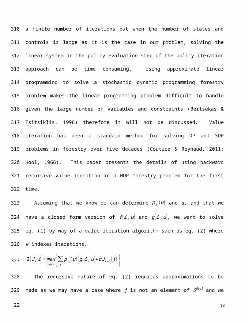
discussed. Value iteration has been a standard method for solving DP and SDP problems in forestry

over five decades (Couture & Reynaud, 2011; Hool, 1966). This paper presents the details of using

backward recursive value iteration in a NDP forestry problem for the first time.

Assuming that we know or can determine pij (u) and α , and that we have a closed form version

of f (i , u ) and g ( i , u ), we want to solve eq. (1) by way of a value iteration algorithm such as eq. (2)

where k indexes iterations.

(2 ) J k (i )=maxuϵU ( i) {∑j

pij (u) [ g ( i ,u )+α J k−1 ( j ) ]}The recursive nature of eq. (2) requires approximations to be made as we may have a case where

j is not an element of SEval and we do not have an exact value for Jk−1 ( j ). Figure 1 illustrates a value

function J plotted against a single state variable where the solid line represents the continuous nature

of the value function, dots represent the values calculated at discreet states i ϵ SEval and X`s represent

values approximated at discrete states j.

In the proposed approach, we replace Jk−1 ( j ) by ~J k−1 ( j , r ) where r is the parameter vector of an

approximation function. We rewrite eq. (2) as:

(3 ) J k ( i )=maxuϵU (i) {∑j

pij (u) [ g ( i ,u )+α ~J k−1 ( j , r ) ] }The fitting approach that leads to the name neuro-dynamic programming is to let r be the

parameters of a neural network architecture. We generalize by letting r be the parameters of any

appropriate continuous function approximating architecture. For example, after calculating Jk (i ) for

all i ϵ SEval at iteration k = 1 of the algorithm, values of Jk ( i ) are grouped by tt and five separate

continuous functions ~J ktt ( i , r ), one for each tt , are fit on values of Jk ( i ). At iteration k = 2, these

11

215

216

217

218

219

220

221

222

223

224

225

226

227

228

229

230

231

232

233

234

235

236

14

continuous functions are used to calculate an approximation ~J k−1tt ( j , r ) for the value of being in state

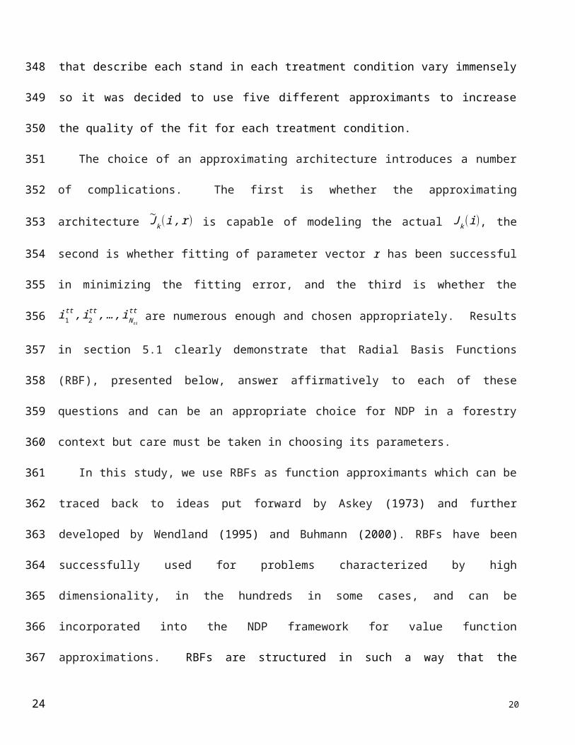
j which is of treatment condition tt . The sets of discrete states that describe each stand in each

treatment condition vary immensely so it was decided to use five different approximants to increase

the quality of the fit for each treatment condition.

The choice of an approximating architecture introduces a number of complications. The first is

whether the approximating architecture ~J k( i , r ) is capable of modeling the actual Jk (i), the second is

whether fitting of parameter vector r has been successful in minimizing the fitting error, and the third

is whether the i1tt ,i2

tt , …,iN tt

tt are numerous enough and chosen appropriately. Results in section 5.1

clearly demonstrate that Radial Basis Functions (RBF), presented below, answer affirmatively to

each of these questions and can be an appropriate choice for NDP in a forestry context but care must

be taken in choosing its parameters.

In this study, we use RBFs as function approximants which can be traced back to ideas put

forward by Askey (1973) and further developed by Wendland (1995) and Buhmann (2000). RBFs

have been successfully used for problems characterized by high dimensionality, in the hundreds in

some cases, and can be incorporated into the NDP framework for value function approximations.

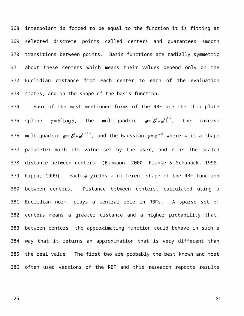
RBFs are structured in such a way that the interpolant is forced to be equal to the function it is fitting

at selected discrete points called centers and guarantees smooth transitions between points. Basis

functions are radially symmetric about these centers which means their values depend only on the

Euclidian distance from each center to each of the evaluation states, and on the shape of the basis

function.

Four of the most mentioned forms of the RBF are the thin plate spline φ=δ 2 log δ, the

multiquadric φ=(δ 2+ω2 )1 /2, the inverse multiquadric φ=(δ 2+ω2 )−1/2, and the Gaussian φ=e−ωδ2

where ω is a shape parameter with its value set by the user, and δ is the scaled distance between

centers (Buhmann, 2000; Franke & Schaback, 1998; Rippa, 1999). Each φ yields a different shape

12

237

238

239

240

241

242

243

244

245

246

247

248

249

250

251

252

253

254

255

256

257

258

259

260

15

of the RBF function between centers. Distance between centers, calculated using a Euclidian norm,

plays a central role in RBFs. A sparse set of centers means a greater distance and a higher

probability that, between centers, the approximating function could behave in such a way that it

returns an approximation that is very different than the real value. The first two are probably the best

known and most often used versions of the RBF and this research reports results using the thin plate

spline which eliminates the need for finding a good value for ω.

Before beginning the value iteration algorithm, we choose a subset of M tt states intt, n=1 ,…, M tt

from each subset tt of SEval which we call centers. After having calculated J (i ) for all i ϵ SEval at

iteration k and having determined that the value iteration algorithm has not converged, we force the

interpolant ~J tt=J ( intt ) at the centers where J (in

tt ) are the values at those centers. M tt is set as a function

of the problem being solved and results will demonstrate the impact of choosing a different number

of centers. The first step is to create, for every tt , a set of M tt equations, one for each intt, using eq.

(4).

(4 ) J ( intt )=∑

m=1

M tt

rmtt φ (|in

tt−imtt|p )for n=1…M tt

We know φ and we use p = 2 as the dimension of the Euclidian norm thus, for every tt , we have

M tt unknowns, the rmtt , and M tt equations giving a linear system A r = f , where the elements of the

M tt × M tt square A matrix are given by φ (|intt−im

tt|2 ) for n=1 …M tt, and the M tt elements of vector f

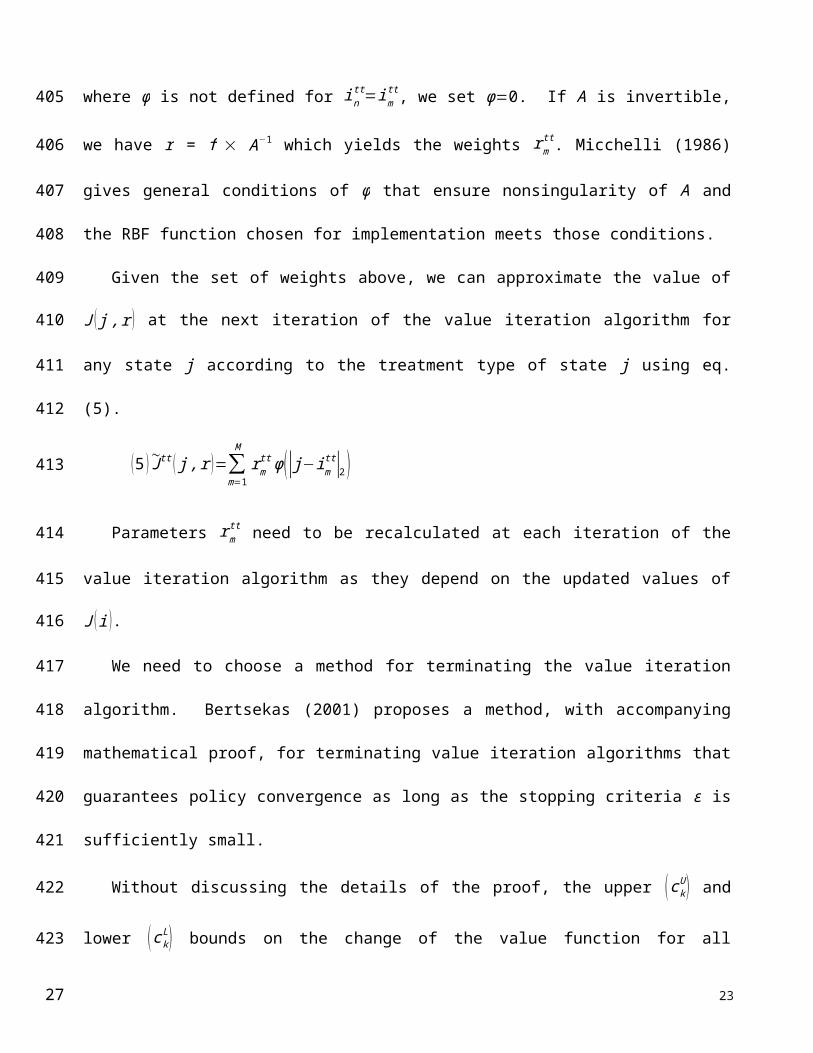
are the values of J (intt ). In the cases where φ is not defined for in

tt=imtt , we set φ=0. If A is invertible,

we have r = f A−1 which yields the weights rmtt . Micchelli (1986) gives general conditions of φ that

ensure nonsingularity of A and the RBF function chosen for implementation meets those conditions.

Given the set of weights above, we can approximate the value of J ( j , r ) at the next iteration of

the value iteration algorithm for any state j according to the treatment type of state j using eq. (5).

13

261

262

263

264

265

266

267

268

269

270

271

272

273

274

275

276

277

278

279

280

281

282

16

(5 ) ~J tt ( j , r )=∑m=1

M

rmtt φ (|j−im

tt|2 )

Parameters rmtt need to be recalculated at each iteration of the value iteration algorithm as they

depend on the updated values of J (i ).

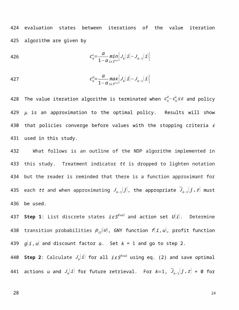
We need to choose a method for terminating the value iteration algorithm. Bertsekas (2001)

proposes a method, with accompanying mathematical proof, for terminating value iteration

algorithms that guarantees policy convergence as long as the stopping criteria ε is sufficiently small.

Without discussing the details of the proof, the upper (ckU ) and lower (ck

L) bounds on the change

of the value function for all evaluation states between iterations of the value iteration algorithm are

given by

ckL= α

1−αminiϵ SEval

[J k (i )−J k−1 (i ) ]

ckU= α

1−αmaxiϵ S Eval

[J k ( i )−J k−1 (i ) ]

The value iteration algorithm is terminated when ckU−ck

L ≤ ε and policy μ is an approximation to the

optimal policy. Results will show that policies converge before values with the stopping criteria ε

used in this study.

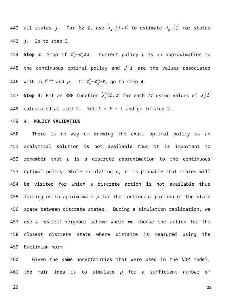
What follows is an outline of the NDP algorithm implemented in this study. Treatment indicator

tt is dropped to lighten notation but the reader is reminded that there is a function approximant for

each tt and when approximating Jk−1 ( j ), the appropriate ~J k−1 ( j , r ) must be used.

Step 1: List discrete states i ϵ SEval and action set U ( i ). Determine transition probabilities pij (u),

GNY function f (i , u ), profit function g (i , u ) and discount factor α . Set k = 1 and go to step 2.

14

283

284

285

286

287

288

289

290

291

292

293

294

295

296

297

298

299

300

301

17

Step 2: Calculate Jk (i ) for all i ϵ SEval using eq. (2) and save optimal actions u and Jk (i ) for future

retrieval. For k=1, ~J k−1 ( j , r ) = 0 for all states j. For k ≥ 2, use ~J k−1 ( j , r ) to estimate Jk−1 ( j ) for

states j. Go to step 3.

Step 3: Stop if ckU−ck

L ≤ ε. Current policy μ is an approximation to the continuous optimal policy and

J¿ ( i ) are the values associated with i ϵ SEval and μ. If ckU−ck

L>ε, go to step 4.

Step 4: Fit an RBF function ~J ktt ( i ,r ) for each tt using values of Jk (i ) calculated at step 2. Set k = k +

1 and go to step 2.

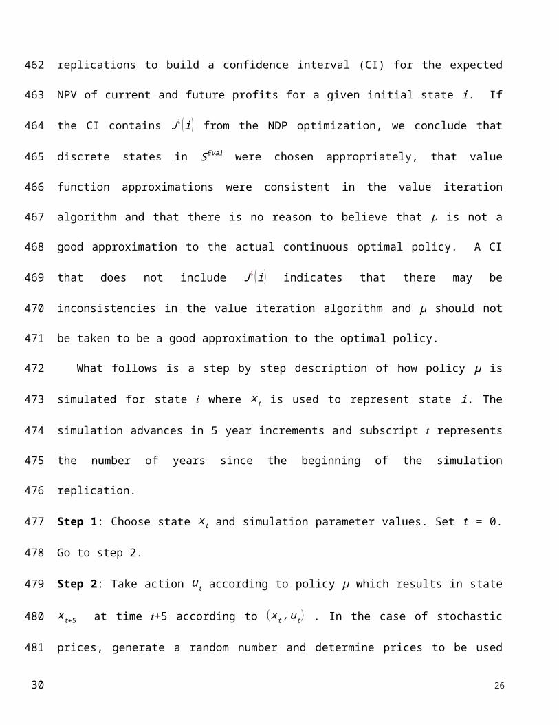
4. POLICY VALIDATION

There is no way of knowing the exact optimal policy as an analytical solution is not available

thus it is important to remember that μ is a discrete approximation to the continuous optimal policy.

While simulating μ, it is probable that states will be visited for which a discrete action is not

available thus forcing us to approximate μ for the continuous portion of the state space between

discrete states. During a simulation replication, we use a nearest-neighbor scheme where we choose

the action for the closest discrete state where distance is measured using the Euclidian norm.

Given the same uncertainties that were used in the NDP model, the main idea is to simulate μ for

a sufficient number of replications to build a confidence interval (CI) for the expected NPV of

current and future profits for a given initial state i. If the CI contains J¿ ( i ) from the NDP

optimization, we conclude that discrete states in SEval were chosen appropriately, that value function

approximations were consistent in the value iteration algorithm and that there is no reason to believe

that μ is not a good approximation to the actual continuous optimal policy. A CI that does not

include J¿ ( i ) indicates that there may be inconsistencies in the value iteration algorithm and μ should

not be taken to be a good approximation to the optimal policy.

15

302

303

304

305

306

307

308

309

310

311

312

313

314

315

316

317

318

319

320

321

322

323

18

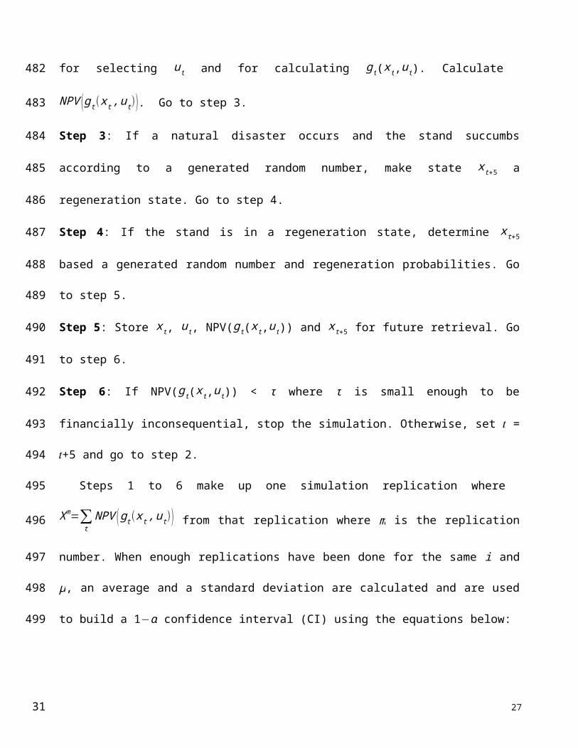
What follows is a step by step description of how policy μ is simulated for state 𝑖 where x t is

used to represent state i. The simulation advances in 5 year increments and subscript 𝑡 represents the

number of years since the beginning of the simulation replication.

Step 1: Choose state x t and simulation parameter values. Set t = 0. Go to step 2.

Step 2: Take action ut according to policy μ which results in state x t+5 at time 𝑡+5 according

to (x t , ut) . In the case of stochastic prices, generate a random number and determine prices to be

used for selecting ut and for calculating gt(x t,ut). Calculate NPV (gt (x t , ut)). Go to step 3.

Step 3: If a natural disaster occurs and the stand succumbs according to a generated random number,

make state x t+5 a regeneration state. Go to step 4.

Step 4: If the stand is in a regeneration state, determine x t +5 based a generated random number and

regeneration probabilities. Go to step 5.

Step 5: Store x t, ut, NPV(gt(x t,ut)) and x t+5 for future retrieval. Go to step 6.

Step 6: If NPV(gt(x t,ut)) < τ where τ is small enough to be financially inconsequential, stop the

simulation. Otherwise, set 𝑡 = 𝑡+5 and go to step 2.

Steps 1 to 6 make up one simulation replication where X m=∑t

NPV (gt (x t , ut)) from that

replication where m is the replication number. When enough replications have been done for the

same i and μ, an average and a standard deviation are calculated and are used to build a 1−α

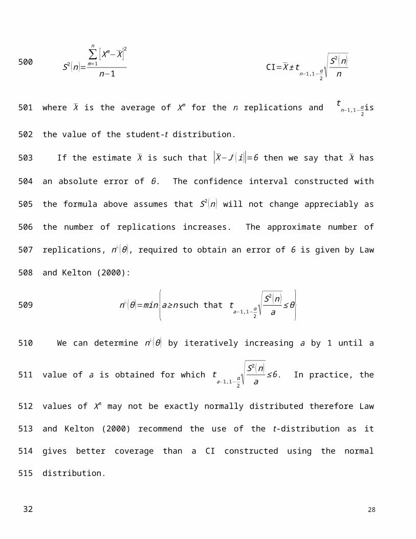
confidence interval (CI) using the equations below:

S2 (n )=∑m=1

n

[ Xm−X ]2

n−1 CI=X ± t

n−1,1−α2 √ S2 (n )

n

where X is the average of X m for the n replications and t n−1,1−α2is the value of the student-t

distribution.

16

324

325

326

327

328

329

330

331

332

333

334

335

336

337

338

339

340

341

342

343

344

19

If the estimate X is such that |X−J¿ ( i )|=ϑ then we say that X has an absolute error of ϑ . The

confidence interval constructed with the formula above assumes that S2 (n ) will not change

appreciably as the number of replications increases. The approximate number of replications, n¿ (ϑ ),

required to obtain an error of ϑ is given by Law and Kelton (2000):

n¿ (ϑ )=min {a ≥ n such that ta−1,1−α

2 √ S2 ( n )a

≤ ϑ }We can determine n¿ (ϑ ) by iteratively increasing a by 1 until a value of a is obtained for which

ta−1,1−α

2 √ S2 (n )a

≤ϑ . In practice, the values of X m may not be exactly normally distributed therefore

Law and Kelton (2000) recommend the use of the t-distribution as it gives better coverage than a CI

constructed using the normal distribution.

Since each discrete state has its corresponding μ ( i ) and J¿ ( i ), any state can be chosen as the

starting point of the simulation and the corresponding J¿ ( i ) compared to the (1-α) CI above. Section

5.3 shows results of CIs constructed for a few discrete states and for different sets of parameters of

the NDP model and discusses the absolute error ϑ for four simulations.

5. RESULTS AND DISCUSSION

All results in this section are for the base case scenario which uses the parameter values in table

2.

5.1 Consistency of function approximations

At each iteration of the value iteration algorithm, the RBF forces ~J=J ( in ) at all centers and

reducing the number of centers can reduce the accuracy of the approximations between the centers.

Distances between centers are calculated using the Euclidian norm with all values of variables scaled

to 0-1.

17

345

346

347

348

349

350

351

352

353

354

355

356

357

358

359

360

361

362

363

364

365

20

Inverting large ill-conditioned matrices can be difficult but scaling of the distances greatly

increases the condition number of the matrix which is an indication of the precision with which it can

be inverted. Reducing the number of centers from a full basis, where all evaluation states are used as

centers, to a reduced basis improves the condition number of the A matrix by many levels of

magnitude. For example, for tt = 2, we have 275 evaluation states. If we scale the distances between

all these states and use all of them as centers in the RBF, the condition number of the matrix is

6.9496 x 107. This is in contrast with an A matrix with 37 centers evenly distributed over the range

of values of the state variables which has a condition number of 5.8042 x 10 4, three orders of

magnitude smaller. But the computational precision gained by having a much better conditioned A

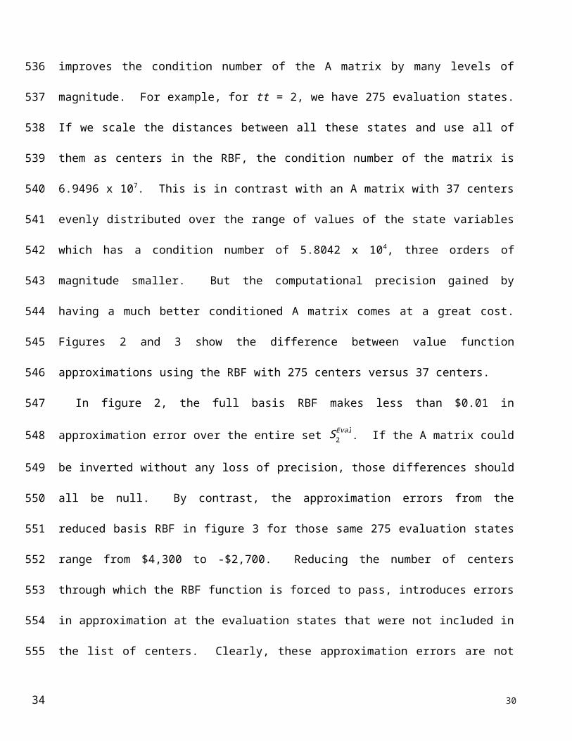
matrix comes at a great cost. Figures 2 and 3 show the difference between value function

approximations using the RBF with 275 centers versus 37 centers.

In figure 2, the full basis RBF makes less than $0.01 in approximation error over the entire set

S2Eval. If the A matrix could be inverted without any loss of precision, those differences should all be

null. By contrast, the approximation errors from the reduced basis RBF in figure 3 for those same

275 evaluation states range from $4,300 to -$2,700. Reducing the number of centers through which

the RBF function is forced to pass, introduces errors in approximation at the evaluation states that

were not included in the list of centers. Clearly, these approximation errors are not acceptable in a

context of NDP where we are trying to iteratively build up values of being in any given state. For this

reason, all results shown in this paper use the full basis thin plate spline RBF approximation

architecture.

5.2 Value iteration algorithm convergence

All optimizations converged in a finite number of iterations and a few examples are presented

below. Table 3 shows results for the base case scenario with the stopping criterion ε=0.2. There is

a clear relationship between the discount rate and the number of iterations to convergence. Table 3

18

366

367

368

369

370

371

372

373

374

375

376

377

378

379

380

381

382

383

384

385

386

387

388

389

21

shows the number of iterations to convergence versus the iteration number of the last policy change.

The iteration number shown in column three is the last iteration during which a policy change was

recorded for any evaluation state. The fourth column of the same table shows the largest value

function change for the last iteration where there is a policy change. Clearly, regardless of the

discount rate, values have not converged when the policy stops changing thus supporting the claim

that as long as ε is sufficiently small, the value iteration algorithm will result in a stable policy that

we show to be optimal through simulation in the next section.

5.3 Monte Carlo policy simulation

Table 4 gives the initial state for the four simulations discussed here. The first three simulations

are done for softwood plantations because, given the parameters used in the NDP, all stands

eventually become softwood plantations. It was important to use different discount rates as well as

deterministic and stochastic prices. The fourth simulation starts with a young natural stand and

allows us to simulate a larger portion of μ.

Simulations 1 and 2 have three price levels so they require the use of random market prices.

Confidence interval (CI) information for the four simulations is given in table 4 as is the number of

replications in each simulation (n¿ (ϑ )). CI`s are built using the average X and standard deviation for

all replications X m for a given simulated μ and starting state i. Simulations 3 and 4 have one price

level therefore the initial market state remains unchanged for the duration of each replication.

As recommended by Law and Kelton (2000), the confidence intervals for these simulations are

constructed using a 95% confidence level and ϑ equivalent to 15% of the optimal value J¿ ( i ) from

the NDP algorithm for the starting state i being simulated. In all cases, confidence intervals contain

J¿ ( i ) for starting state i and policy μ but the intervals are quite wide because of the suggested large

value of ϑ . The 15% value suggested by Law and Kelton is very conservative for our purposes and

leads to very wide confidence intervals that are not very useful. If ϑ was reduced until the 95% CI

19

390

391

392

393

394

395

396

397

398

399

400

401

402

403

404

405

406

407

408

409

410

411

412

413

22

was too narrow to include J¿ (i ), we would have ϑ < 5.2% for all simulations. We can say with 95%

confidence and a relatively small absolute error, that μ is a good approximation to the continuous

optimal policy in those four cases.

5.4 Policy discussion

The policy discussion presented here is not meant to be a complete interpretation of the

implications of using the policies calculated using NDP but rather some observations to reflect the

level of detail obtained by using the methods described in this paper.

All states in the left side of table 5 are natural unmanaged stands (tt=1) and they are discrete

elements of SEval, and all states in the right side of the table are either pre-commercially (tt=2) or

commercially thinned (tt=5) stands. Each of the colour-coded numbers makes reference to an action

to be applied to the stand. A pre-commercial thinning action takes the stand from tt=1 tott=2 and a

commercial thinning action applied to a natural unmanaged stand takes the stand from tt=1 to tt=5.

The reader is reminded that the natural stands on the left have 100% crown closure on a 100%

stocked stand therefore the stand is supporting as many trees as it possibly can for its age. These

natural stands have an average SW content of 75%. What follows is an example of the level of detail

we can get from using NDP to develop individual stand management policies.

Action 1 is to do nothing and let the stand grow for one 5-year period. In all cases, taking action

1 simply means the stand will be 5 years older at the next decision time. For 5 year old natural

stands, it is optimal to do nothing as the trees are too short to do a pre-commercial thinning and the

diameters are too small to have any commercial value. Action 12 is a pre-commercial thinning that

eliminates hardwood and spaces softwood to NS DNR recommended spacing and it is optimal to

apply this action regardless of market price at ages 10 and 15. Taking action 12 with 10 and 15 year

old natural stands, and letting them grow 5 years, results in transitions to the first two stands

respectively (stands 1 and 2) in the right side of table 5. We notice that the new stands have had all

20

414

415

416

417

418

419

420

421

422

423

424

425

426

427

428

429

430

431

432

433

434

435

436

437

23

their hardwood removed (pct S = 100%) and that the new crown closure percentage is very low. In

both cases, it is optimal to do nothing and let the stand grow (action 2) regardless of the observed

state of the market. As random disturbances occur and the state of the forest stand and market

evolve, the policies are used to continually make optimal decisions based on the state observed at

decision time.

By age 20, an unmanaged natural stand has self-thinned to a point that investing in a PCT to thin

out the stand is no longer the optimal action to take. Therefore, between the ages of 20 and 30

inclusively, it is optimal to do nothing and let the stand grow. At those ages, the average diameter of

the trees is still too small to have any commercial value.

All optimal CT actions remove 40% of the total basal area on the stand and, aside from a few

exceptions, CT actions are clustered into two groups. The first group, actions 19, 28 and 37, all

remove the basal area by taking it as 25% SW and 75% HW. The only difference is the manner in

which it is taken where 19 takes trees from the small diameters (from below), 28 takes the trees from

across the diameter distribution and 37 takes the trees from the largest diameters (from above). In

the second group, actions 38 and 39, CT is done from above with 50% basal area removal that is

75% SW with the balance in HW. Doing a commercial thinning from above yields slightly higher

volumes for the same basal area but, more importantly, it creates a larger proportion of large logs

which has a much higher market value, and higher market prices encourage the removal of larger

trees because there is a high probability that prices will come down at the next period. The majority

of the CT actions in the policy from the left hand side of table 5 lead to a state where the optimal

action is to do nothing for at least 5 years. Stands 3 to 13 from the right side of table 6 are a

sampling of the resulting forest stands after taking actions 19, 28, 37, 38 or 39 with the natural stands

in the left side of table 5. Two characteristics are similar for all these stands: pct S =100% for all

stands except stand 3 which still contains a small percentage of HW and cc varies within a narrow

21

438

439

440

441

442

443

444

445

446

447

448

449

450

451

452

453

454

455

456

457

458

459

460

461

24

range of 44% to 52%. At such low cc, it makes no sense to remove any trees as the amount of

timber does not justify the removal. The policies in the right side of table 5 reflect this as it is optimal

to do nothing for all stands up to 60 years of age (state 10). Starting at age 65, some regeneration

harvests appear at very high prices with more appearing at age 75 (state 14). At this age, the stand

diameter is high enough that it is optimal to do a regeneration harvest if the prices are simply above

the mean. States 14 and 15 are shown to demonstrate that doing nothing when in state 14 yields state

15, and that with the rise in cc and diameter, there is a significant change in policy in just 5 years.

6. CONCLUSION

The main objective of this study as stated in the introduction is to demonstrate how to use a

neuro-dynamic programming approach to the stand management problem when faced with high

dimensional state and control spaces as well as multiple sources of uncertainty. For the same

number of possible outcomes for each source of uncertainty, SDP typically requires a much higher

number of discrete states because NDP can approximate the profit function between discrete states

without sacrificing accuracy. In NDP, profit function approximations are built into the algorithm

allowing for a much higher number of possible outcomes from all sources of uncertainty without

needing to increase the number of discrete states. The set of state variables used in this study is not

sufficient to fully model the management of real forest stands but it begins to approach the level of

detail that forest managers might consider while developing policies. However, the detailed

state/action spaces allow us to start considering the impact of uncertainty from sources such as the

difference between planned harvest volumes and actual volumes, uncertain growth projections,

climate change or uncertain quality of wood products at harvest.

Real world problems where many sources of uncertainty affect expected state/action outcomes

and which would benefit from an additional level of detail in the optimal policies may be revisited

using the ideas of NDP. Problems that could benefit from NDP typically are modeled using

22

462

463

464

465

466

467

468

469

470

471

472

473

474

475

476

477

478

479

480

481

482

483

484

485

25

stochastic dynamic programming and have a state space that can be represented by a sparse set of

discrete states without loosing the level of detail necessary to capture policy changes. To see NDP

gain wider use in forestry, we must take a closer look at problems that would typically be solved

using SDP algorithms but would be modeled with a simplified representation of uncertainty in its

SDP form. The main reason for incorporating uncertainty in forestry models is to quantify risk in

order to make informed decisions. Methodologies such as NDP can capture the dynamics of real

decision making while simultaneously considering as many sources of uncertainty as possible so that

policies are reasonable representations of real life decisions and can be used to create useful policy

discussions.

Forestry will continue to pose important problems that involve the solution of large scale

stochastic dynamic programming problems. Neuro-dynamic programming is an approach that shows

considerable promise.

Acknowledgements

This work was partially supported through a Discovery Grant from the Natural Sciences and

Engineering Research Council of Canada. Dr. Jules Comeau was supported in part by a scholarship

from the Baxter and Alma Ricard Foundation.

References

Amacher, G. S., Ollikainen, M., & Koskela, E. (2009). Economics of Forest Resources. Cambridge,

Massachussetts: MIT Press.

Amidon, E. L., & Akin, G. S. (1968). Dynamic Programming to Determine Optimum Levels or

Growing Stock. Forest Science, 14(3), 287–291.

23

486

487

488

489

490

491

492

493

494

495

496

497

498

499

500

501

502

503

504

505

26

Arthaud, G. J., & Klemperer, W. D. (1988). Optimizing high and low thinnings in loblolly pine with

dynamic programming. Canadian Journal of Forest Research, 18, 1118–1122.

https://doi.org/10.1139/x88-172

Askey, R. (1973). Radial characteristic functions (Mathematics Research Center Report No. 1262).

University of Wisconsin.

Bertsekas, D. P. (2001). Dynamic Programming and Optimal Control (2nd ed., Vol. 2). Belmont,

Massachusetts: Athena Scientific.

Bertsekas, D. P., & Tsitsiklis, J. N. (1996). Neuro-Dynamic Programming (2nd ed.). Belmont,

Massachusetts: Athena Scientific.

Brodie, J. D., Adams, D. M., & Kao, C. (1978). Analysis of Economic Impacts on Thinning and

Rotation for Douglas-fir, Using Dynamic Programming. Forest Science, 24(4), 513–522.

Brodie, J. D., & Kao, C. (1979). Optimizing Thinning in Douglas-fir with Three-Descriptor Dynamic

Programming to Account for Accelerated Diameter Growth. Forest Science, 25(4), 665–672.

Buhmann, M. D. (2000). Radial Basis Functions. Acta Numerica, 9, 1–38.

Canadian Forest Service. (1995). Silvicultural Terms in Canada. Retrieved from

http://nfdp.ccfm.org/terms/terms_e.php

Castelletti, A., de Rigo, D., Rizzoli, A. E., Soncini-Sessa, R., & Weber, E. (2007). Neuro-dynamic

programming for designing water reservoir network management policies. Control

Engineering Practice, 15(8), 1031–1038. https://doi.org/10.1016/j.conengprac.2006.02.011

Chen, C. M., Rose, D. W., & Leary, R. A. (1980). How to formulate and solve “optimal stand

density over time” problems for even-aged stands using dynamic programming (No. General

technical report NC-56) (p. 17). US Department of Agriculture Forest Service.

24

506

507

508

509

510

511

512

513

514

515

516

517

518

519

520

521

522

523

524

525

526

527

27

Couture, S., & Reynaud, A. (2011). Forest management under fire risk when forest carbon

sequestration has value. Ecological Economics, 70(11), 2002–2011.

https://doi.org/10.1016/j.ecolecon.2011.05.016

Davis, L. S., Johnson, K. N., Bettinger, P., & Howard, T. E. (2005). Forest Management To sustain

Ecological, Economic, and Social Values (4th ed.). Long Grove, Il: Waveland Press Inc.

Department of Natural Resources of Nova Scotia. (1993). Forestry Field Handbook (p. 43).

Retrieved from http://novascotia.ca/natr/forestry/handbook/

Faustmann, M. (1849). Calculation of the value which forest land and immature stands possess for

forestry (Institute paper No. 42). Commonwealth Forest Institute, University of Oxford.

Ferreira, L., Constantino, M. F., Borges, J. G., & Garcia-Gonzalo, J. (2012). A Stochastic Dynamic

Programming Approach to Optimize Short-Rotation Coppice Systems Management

Scheduling: An Application to Eucalypt Plantations under Wildfire Risk in Portugal. Forest

Science, 58(4), 353–365. https://doi.org/10.5849/forsci.10-084

Forboseh, P. F., & Pickens, J. B. (1996). A Reservation Value Approach to Harvest Scheduling with

Stochastic Stumpage Prices. Forest Science, 42(4), 465–473.

Franke, C., & Schaback, R. (1998). Solving partial differential equations by collocation using radial

basis functions. Applied Mathematics and Computation, 93(1), 73–82.

https://doi.org/10.1016/S0096-3003(97)10104-7

Gunn, E. A. (2005). A neuro-dynamic programming approach to the optimal stand management

problem. In M. Bevers & T. M. Barrett (Eds.), System analysis in forest resources:

proceedings of the 2003 symposium (Vol. Gen. Tech. Rep. PNW-GTR-656, p. 366).

Stevenson, Washington, US. Retrieved from

http://www.fs.fed.us/pnw/publications/pnw_gtr656/

25

528

529

530

531

532

533

534

535

536

537

538

539

540

541

542

543

544

545

546

547

548

549

550

28

Haight, R. G. (1990). Feedback Thinning Policies for Uneven-Aged Stand Management with

Stochastic Prices. Forest Science, 36(4), 1015–1031.

Haight, R. G., Brodie, J. D., & Dahms, W. G. (1985). A Dynamic Programming Algorithm for

Optimization of Lodgepole Pine Management. Forest Science, 31(2), 321–330.

Haight, R. G., & Holmes, T. P. (1991). Stochastic price models and optimal tree cutting: results for

loblolly pine. Natural Resource Modeling, 5(4), 423–443.

Hanewinkel, M., Hummel, S., & Albrecht, A. (2011). Assessing natural hazards in forestry for risk

management: a review. European Journal of Forest Research, 130(3), 329–351.

https://doi.org/http://dx.doi.org.proxy.cm.umoncton.ca/10.1007/s10342-010-0392-1

Hildebrandt, P., & Knoke, T. (2011). Investment decisions under uncertainty—A methodological

review on forest science studies. Forest Policy and Economics, 13(1), 1–15.

https://doi.org/10.1016/j.forpol.2010.09.001

Hool, J. N. (1966). A Dynamic Programming - Markov Chain Approach to Forest Production

Control. (E. L. Stone, Ed.) (Vol. 12). Washington, D.C.: Society of American Foresters.

Ilkova, T., Petrov, M., & Roeva, O. (2012). Optimization of a Whey Bioprocess using Neuro-

Dynamic Programming Strategy. Biotechnology & Biotechnological Equipment, 26(5),

3249–3253. https://doi.org/10.5504/BBEQ.2012.0063

Law, A. M., & Kelton, W. D. (2000). Simulation Modeling and Analysis (3rd ed.). McGraw Hill.

Lembersky, M. R., & Johnson, K. N. (1975). Optimal Policies for Managed Stands: An Infinite

Horizon Markov Decision Process Approach. Forest Science, 21(2), 109–122.

Lien, G., Stordal, S., Hardaker, J. B., & Asheim, L. J. (2007). Risk aversion and optimal forest

replanting: A stochastic efficiency study. European Journal of Operational Research, 181,

1584–1592. https://doi.org/10.1016/j.ejor.2005.11.055

26

551

552

553

554

555

556

557

558

559

560

561

562

563

564

565

566

567

568

569

570

571

572

573

29

Lu, F., & Gong, P. (2003). Optimal stocking level and final harvest age with stochastic prices.

Journal of Forest Economics, 9(2), 119–136. https://doi.org/10.1078/1104-6899-00026

McGrath, T. (1993). Nova Scotia Softwood Growth and Yield Model - Version 1.0 User Manual

(Forest Research Report No. 43). Forest Research Section, Forestry Branch, N.S. Dept. of

Natural Resources. Retrieved from

http://novascotia.ca/natr/library/forestry/reports/report43.pdf

Micchelli, C. A. (1986). Interpolation of Scattered Data: Distance Matrices and Conditionally

positive definite Functions. Constructive Approximation, 2, 11–22.

https://doi.org/10.1007/BF01893414

Näslund, B. (1969). Optimal Rotation and Thinning. Forest Science, 15(4), 446–451.

Nicol, S., & Chadès, I. (2011). Beyond stochastic dynamic programming: a heuristic sampling

method for optimizing conservation decisions in very large state spaces. Methods in Ecology

and Evolution, 2(2), 221–228. https://doi.org/10.1111/j.2041-210X.2010.00069.x

Nova Scotia department of lands and forests. (1990). Revised normal yield tables for Nova Scotia

softwoods (Research Report No. 22) (pp. 1–46). Nova Scotia Department of Lands and

Forests. Retrieved from http://novascotia.ca/natr/library/forestry/reports/report22.pdf

Nova Scotia Department of Natural Resources. (1996). Honer’s Standard Volume Table Estimates

Compared to Nova Scotia Stem Analyses. Retrieved from

http://novascotia.ca/natr/library/forestry/reports/report61.pdf

O’Keefe, R. N., & McGrath, T. P. (2006). Nova Scotia Hardwood Growth and Yield Model (No.

FOR 2006-2 No. 78). Retrieved from

http://novascotia.ca/natr/library/forestry/reports/REPORT78.PDF

Peltola, J., & Knapp, K. C. (2001). Recursive Preferences in Forest Management. Forest Science,

47(4), 455–465.

27

574

575

576

577

578

579

580

581

582

583

584

585

586

587

588

589

590

591

592

593

594

595

596

597

30

Rios, I., Weintraub, A., & Wets, R. J.-B. (2016). Building a stochastic programming model from

scratch: a harvesting management example. Quantitative Finance, 16(2), 189–199.

https://doi.org/10.1080/14697688.2015.1114365

Rippa, S. (1999). An algorithm for selecting a good value for the parameter c in radial basis function

interpolation. Advances in Computational Mathematics, 11, 193–210.

https://doi.org/10.1023/A:1018975909870

Schreuder, G. (1971). The Simultaneous Determination of Optimal Thinning Schedule and Rotation

for an Even-Aged Forest. Forest Science, 17, 333–339.

Steenberg, J. W. N., Duinker, P. N., & Bush, P. G. (2012). Modelling the effects of climate change

and timber harvest on the forests of central Nova Scotia, Canada. Annals of Forest Science,

70(1), 61–73. https://doi.org/10.1007/s13595-012-0235-y

Sutton, R. S., & Barto, A. G. (1998). Reinforcement Learning (1st ed.). Cambridge, MA: MIT Press.

Retrieved from https://mitpress.mit.edu/books/reinforcement-learning

von Gadow, K. (Ed.). (2001). Risk Analysis in Forest Management (1st ed., Vol. 1). Dordrecht /

Boston / London: Kluwer Academic Publishers.

Wendland, H. (1995). Piecewise polynomial, positive definite and compactly supported radial

functions of minimal degree. Advances in Computational Mathematics, 4(1), 389–396.

https://doi.org/10.1007/BF02123482

Yoshimoto, A. (2002). Stochastic Control Modeling for Forest Stand Management under Uncertain

Price Dynamics through Geometric Brownian Motion. Journal of Forest Research, 7, 81–90.

https://doi.org/10.1007/BF02762512

Yoshimoto, A., Asante, P., & Konoshima, M. (2016). Stand-Level Forest Management Planning

Approaches. Current Forestry Reports, 2(3), 163–176. https://doi.org/10.1007/s40725-016-

0041-0

28

598

599

600

601

602

603

604

605

606

607

608

609

610

611

612

613

614

615

616

617

618

619

620

621

31

Yousefpour, R., Jacobsen, J. B., Thorsen, B. J., Meilby, H., Hanewinkel, M., & Oehler, K. (2012). A

review of decision-making approaches to handle uncertainty and risk in adaptive forest

management under climate change. Annals of Forest Science, 69(1), 1–15.

https://doi.org/10.1007/s13595-011-0153-4

Table 1 – Range of values for state variables where S = softwood and H = hardwoodtt = 1

Natural unmanaged

tt = 2PCT natural

tt = 3Softwood plantation

tt = 4CT plantation

tt = 5CT natural

min max min max min max min max min maxAge (years) 0 95 5 95 5 95 10 100 25 105

st % 75 100 - - - - - - - - - - - - - - - -ipd

(trees/hectare)- - - - - - - - 1000 4000 - - - - - - - -

dS (cm) - - - - 5.3 30.8 0 28.1 3.9 33.4 8.5 37.2

d H (cm) - - - - 1.1 20.7 - - - - - - - - 6.8 28.3

pct S (%) - - - - 0 100 - - - - - - - - 0 100

cc (%) - - - - 5.7 100 - - - - 40 100 40 100# discreet states 38 275 76 90 648

Table 2 – Basic parameters of the NDP modelAnnual discount rate 2%Site index SW (in meters at age 50) 16.76mSite index HW (in meters at age 50) 17mMinimum dominant stand height (hardwood) for doing a pre-commercial thinning 6.1mMinimum dominant stand height (softwood) for doing a pre-commercial thinning 2mMaximum average stand height for doing a pre-commercial thinning 9mPercentage of stand covered with softwood when a stand does naturally regenerate 75%Natural stocking percentage of the forest 75%Average selling price of softwood merchantable volume $13.07/m3

Average selling price of softwood board volume $30.76/m3

Average selling price of hardwood merchantable volume $22.40/m3

Average selling price of hardwood board volume $46.23/m3

Number of price level 1Cost of planting less than 2500 trees on one hectare $1,350Cost of planting 2500 or more trees on one hectare $1,500Cost of surveying one hectare of newly harvested land $70Cost of doing fill planting on one hectare $300Cost of doing pre-commercial thinning on one hectare $750Cost of one hour of labour for doing commercial thinning or final felling $40

29

622

623

624

625

626

627628629630

32

Flat cost of doing a commercial thinning on one hectare $750Approximate forested area in the west of the province of Nova Scotia (hectares) 1,691,300Average number of fires per year in the area under study 3.5Return interval of major hurricanes (years) 50Average area of wind for a major hurricane (hectares) 400,000Return interval of major insect outbreaks (years) 50

Table 3 – Example results for the base case scenario with thin plate spline RBF approximation and stopping criterion ε = 0.2

Table 4 – Details of four Monte Carlo policy simulations including 95% confidence interval and number of replicationsSim α # of price

breaksReplication

lengthStarting state Lower CI Upper CI DP value

function J*n¿ (ϑ )

TRT Age Initialdensity

1 0.04 3 295 years 3 25 2500 $2,838.79 $3,862.56 $3,403.40 292 0.04 3 295 years 3 35 3250 $3,263.89 $10,376.53 $6,945.36 23 0.03 1 295 years 3 30 2500 $4,352.78 $6,254.93 $4,890.85 44 0.02 1 695 years 1 15 n/a $9,606.29 $12,998.07 $11,399.81 19

30

α (%) # iterations for convergence

Iteration # of last policy change

Largest value function change at last policy change

1.0 138 105 $110.552.0 101 42 $287.114.0 39 23 $14.11

631

632

633

634635636

637

638

639

640

641642

643644

33

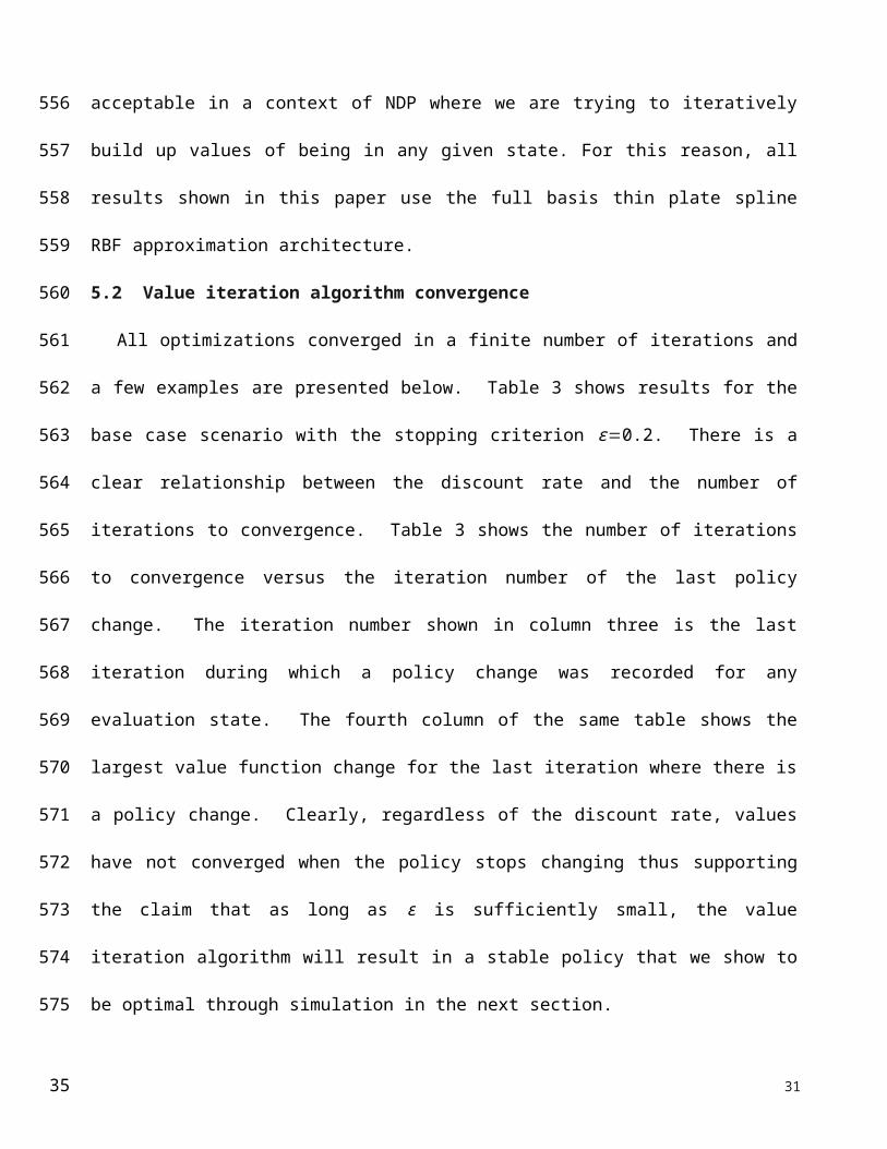
Table 5 – Partial policies for the base case scenario with 6 price levelsNatural unmanaged stands Commercially or pre-commercially thinned natural stands

Age

(yea

rs)

Stoc

king

(%)

Pric

e 1

Pric

e 2

Pric

e 3

Pric

e 4

Pric

e 5

Pric

e 6

Stan

d nu

mbe

r

Age

(yea

rs)

dS

(cm

)

d H

(cm

)

pct S

(%)

cc

(%)

Pric

e 1

Pric

e 2

Pric

e 3

Pric

e 4

Pric

e 5

Pric

e 6

5 100 1 1 1 1 1 1 1 15 5.2 0 100 8.4 2 2 2 2 2 210 100 12 12 12 12 12 12 2 20 6.9 0 100 14.1 2 2 2 2 2 215 100 12 12 12 12 12 12 3 40 8.7 7.0 92 46.5 2 2 2 2 2 220 100 1 1 1 1 1 1 4 45 10.6 0 100 44.5 2 2 2 2 2 225 100 1 1 1 1 1 1 5 50 12.1 0 100 44.7 2 2 2 2 2 230 100 1 1 1 1 1 1 6 55 13.5 0 100 44.9 2 2 2 2 2 235 100 1 1 39 39 39 39 7 55 15.0 0 100 51.1 2 2 2 2 2 240 100 1 38 38 38 38 38 8 55 14.0 0 100 51.6 2 2 2 2 2 245 100 38 38 38 38 38 38 9 60 15.0 0 100 45.0 2 2 2 2 2 250 100 19 19 37 38 38 38 10 60 15.4 0 100 51.8 2 2 2 2 2 255 100 37 37 37 37 38 7 11 65 16.8 0 100 51.9 2 2 2 2 2 760 100 28 37 37 37 7 7 12 70 18.2 0 100 52.1 2 2 2 2 2 765 100 37 37 37 7 7 7 13 75 19.4 0 100 52.2 2 2 2 7 7 770 100 1 37 7 7 7 775 100 1 1 7 7 7 7 14 65 17.4 0 100 51.7 2 2 2 2 2 780 100 1 1 7 7 7 7 15 70 22.0 0 100 59 2 2 2 7 7 785 100 1 1 7 7 7 790 100 1 1 7 7 7 7 16 100 27.2 0 100 52.0 2 2 7 7 7 795 100 19 19 7 7 7 7

1 - Let grow 12 - PCT, remove HW 37 - CT, rmv 40% BA, splt 25% (abv) 2 - Let grow 19 - CT, rmv 40% BA, splt 25% (blw) 38 - CT, rmv 40% BA, splt 50% (abv) 7 - ReHar, plt 2500 tr/ha 28 - CT, rmv 40% BA, splt 25% (cros) 39 - CT, rmv 40% BA, splt 75% (abv)

31

645

646

647

648

649

650

34

Figure 1 – Representation of a value function. The solid line represents the continuous nature of the value function, the dots represent the values calculated at a discreet states i ϵ SEval and X`s represent values approximated at discrete states j.

Figure 2 - Difference between approximate value and actual value, plotted against age, for the 275 discrete states for TRT=2 with those 275 states being used as centers in the RBF with distances scaled to 0-1

Figure 3 – Difference between approximate value and actual value, plotted against age, for the 275 discrete states for TRT=2 with 37 states being used as centers in the RBF with distances scaled to 0-1

3235

Figure 1

Figure 2

33

0 10 20 30 40 50 60 70 80 90 100-0.008

-0.006

-0.004

-0.002

0

0.002

0.004

0.006

0.008

0.01

Age (years)

Diff

eren

ce ($

)

36

Figure 3

34

0 10 20 30 40 50 60 70 80 90 100-4000

-3000

-2000

-1000

0

1000

2000

3000

4000

5000

Age (years)

Diff

eren

ce ($

)

37