0 analysis and architecture design of variable block...

0

Analysis and Architecture Design of Variable

Block Size Motion Estimation for H.264/AVC

Ching-Yeh Chen, Shao-Yi Chien, Yu-Wen Huang, Tung-Chien Chen, Tu-Chih

Wang, and Liang-Gee Chen

August 16, 2005 DRAFT

1

Manuscript received

Affiliation of Authors

Ching-Yeh Chen, Shao-Yi Chien, Yu-Wen Huang, Tung-Chien Chen, Tu-Chih Wang, and Prof.

Liang-Gee Chen are with DSP/IC Design Lab., Graduate Institute of Electronics Engineering

and Department of Electrical Engineering, National TaiwanUniversity, Taipei, Taiwan. Tu-Chih

Wang is also with Chin Fong Machine Industrial, Chang Hua, Taiwan.

Corresponding Author:

Ching-Yeh Chen

Address:

Room 332, Department of Electrical Engineering II, National Taiwan University

1, Sec. 4, Roosevelt Rd., Taipei 10617, Taiwan

Email: [email protected]

Tel: +886-2-23635251ext332

Fax: +886-2-23681679


2

Abstract

Variable block size motion estimation (VBSME) has become animportant video coding technique,

but it increases the difficulty of hardware design. In this paper, we use inter/intra-level classification

and various data flows to analyze the impact of supporting VBSME in different hardware architectures.

Furthermore, we propose two hardware architectures, whichcan support traditional fixed block size

motion estimation as well as VBSME with the less chip area overhead compared to previous approaches.

By broadcasting reference pixel rows and propagating partial SADs, the first design has the fewer

reference pixel registers and a shorter critical path. The second design utilizes a 2-D distortion array

and one adder tree with the reference buffer which can maximize the data reuse between successive

searching candidates. The first design is suitable for the low resolution or small search range, and

the second design has advantages of supporting a high degreeof parallelism and VBSME. Finally,

we propose an eight-parallel SAD tree with shared referencebuffer for H.264/AVC integer motion

estimation (IME). Its processing ability is eight times of the single SAD tree, but the reference buffer

size is only doubled. Moreover, the most critical issue of H.264 IME, huge memory bandwidth, is

overcome. 99.9% off-chip memory bandwidth and 99.22% on-chip memory bandwidth are saved. We

demonstrate a 720p, 30fps solution at 108 MHz with 330.2K gate count and 208K bits on-chip memory.

Index Terms

H.264/AVC, motion estimation, block matching, variable block size, VLSI architecture.

I. INTRODUCTION

For video coding systems, motion estimation (ME) can removemost of temporal redundancy,

so a high compression ratio can be achieved. Among various MEalgorithms, full search block

matching algorithm (FSBMA) is usually adopted because of its good quality and regular com-

putation. In FSBMA, the current frame is partitioned into many small macroblocks (MB) of size

N×N. For each MB in the current frame (current MB), one referenceblock which is the most

similar to current MB is looked for in the searching range of size [−P,P) in the reference frame.

The most common used criterion of the similarity is the sum ofabsolute differences (SAD),

SAD(m,n) =N

∑i=1

N

∑j=1

Distortion(i, j,m,n), −P≤ m,n < P, (1)

Distortion(i, j,m,n) = |cur(i, j)− re f(i +m, j +n)| , (2)


3

wherecur(i, j) andre f(i +m, j +n) are pixel values in current MB (current pixel) and reference

block (reference pixel),(m,n) is one searching candidate in search range,Distortion(i, j,m,n)

is the difference between current pixel and reference pixel, andSAD(m,n) is the total distortion

of this searching candidate. The row (column) SAD is the summation of N distortions in a

row (column). After all searching candidates are examined,the searching candidate which has

the smallest SAD is selected as the motion vector of current MB. Although FSBMA provides

the best quality among various ME algorithms, it consumes the largest computation power. In

general, the computation complexity of ME is from 50% to 90% of a typical video coding

system. Hence a hardware accelerator of ME is required.

Variable block size motion estimation (VBSME) is a new coding technique and provides

more accurate predictions compared to traditional fixed block size motion estimation (FBSME).

With FBSME, if a MB consists of two objects with different motion directions, the coding

performance of this MB is worse. On the other hand, for the same condition, the MB can be

divided into smaller blocks in order to fit the different motion directions with VBSME. Hence the

coding performance is improved. VBSME has been adopted in the latest video coding standards,

including H.263 [1], MPEG-4 [2], WMV9.0 [3], and H.264/AVC [4]. For instance, in H.264/AVC,

a MB with variable block size can be divided into seven kinds of blocks including 4×4, 4×8,

8×4, 8×8, 8×16, 16×8, and 16×16. Although VBSME can achieve higher compression ratio,

it not only requires huge computation complexity but also increases the difficulty of hardware

implementation for ME.

Traditional ME hardware architectures are designed for FBSME, and they can be classified

into two categories. One is an inter-level architecture, where each processing element (PE) is

responsible for one SAD of a specific searching candidate, asshown in (1), and the other is an

intra-level architecture, where each PE is responsible forthe distortion of a specific current pixel

in the current MB for all searching candidates, as shown in (2). For example, Yang, Sun, and

Wu proposed an 1-D inter-level semisystolic architecture [5], and Komarek and Pirsch proposed

a 2-D intra-level systolic architecture, AB2, in [6].

In this paper, we not only use inter/intra-level classification and various data flows to analyze

the impact of supporting VBSME in different hardware architectures but also propose two

hardware architectures,Propagate Partial SADandSAD Tree, which can support VBSME as well

as FBSME with the less chip area overhead compared to previous techniques. After analyzing


4

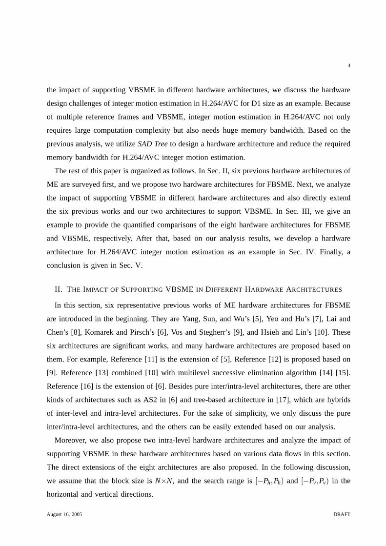
the impact of supporting VBSME in different hardware architectures, we discuss the hardware

design challenges of integer motion estimation in H.264/AVC for D1 size as an example. Because

of multiple reference frames and VBSME, integer motion estimation in H.264/AVC not only

requires large computation complexity but also needs huge memory bandwidth. Based on the

previous analysis, we utilizeSAD Treeto design a hardware architecture and reduce the required

memory bandwidth for H.264/AVC integer motion estimation.

The rest of this paper is organized as follows. In Sec. II, sixprevious hardware architectures of

ME are surveyed first, and we propose two hardware architectures for FBSME. Next, we analyze

the impact of supporting VBSME in different hardware architectures and also directly extend

the six previous works and our two architectures to support VBSME. In Sec. III, we give an

example to provide the quantified comparisons of the eight hardware architectures for FBSME

and VBSME, respectively. After that, based on our analysis results, we develop a hardware

architecture for H.264/AVC integer motion estimation as anexample in Sec. IV. Finally, a

conclusion is given in Sec. V.

II. THE IMPACT OF SUPPORTINGVBSME IN DIFFERENT HARDWARE ARCHITECTURES

In this section, six representative previous works of ME hardware architectures for FBSME

are introduced in the beginning. They are Yang, Sun, and Wu’s[5], Yeo and Hu’s [7], Lai and

Chen’s [8], Komarek and Pirsch’s [6], Vos and Stegherr’s [9], and Hsieh and Lin’s [10]. These

six architectures are significant works, and many hardware architectures are proposed based on

them. For example, Reference [11] is the extension of [5]. Reference [12] is proposed based on

[9]. Reference [13] combined [10] with multilevel successive elimination algorithm [14] [15].

Reference [16] is the extension of [6]. Besides pure inter/intra-level architectures, there are other

kinds of architectures such as AS2 in [6] and tree-based architecture in [17], which are hybrids

of inter-level and intra-level architectures. For the sakeof simplicity, we only discuss the pure

inter/intra-level architectures, and the others can be easily extended based on our analysis.

Moreover, we also propose two intra-level hardware architectures and analyze the impact of

supporting VBSME in these hardware architectures based on various data flows in this section.

The direct extensions of the eight architectures are also proposed. In the following discussion,

we assume that the block size isN×N, and the search range is[−Ph,Ph) and [−Pv,Pv) in the

horizontal and vertical directions.


5

A. Yang, Sun, and Wu’s

Yang, Sun, and Wu implemented the first VLSI motion estimatorin the world, as shown

in Fig. 1(a), which is an 1-D inter-level hardware architecture (1DInterYSW). The number of

PEs is equal to the number of searching candidates in the horizontal direction, 2Ph. Reference

pixels are broadcasted into all PEs. By selection signals, the corresponding reference pixel is

selected and inputted into each PE. Current pixels are propagated with propagation registers,

and the partial SAD is stored in each PE. In each cycle, each PEcomputes the distortion and

accumulates the SAD of a searching candidate. In this architecture, the most important concept

is data broadcasting. With broadcasting technique, the memory bitwidth which is defined as the

number of bits for the required reference data in one cycle isreduced significantly, although

some global routings are required.

B. Yeo and Hu’s

Figure 1(b) shows a 2-D inter-level hardware architecture which is proposed by Yeo and Hu

(2DInterYH). 2DInterYH consists of 2Ph×2Pv PEs and is similar to 1DInterYSW. Reference

pixels are broadcasted into PEs, and current pixels are propagated with propagation registers.

The partial SADs are stored and accumulated in PEs, respectively. Because of broadcasting

reference pixels in both directions, the number of PEs has tomatch the MB size. Hence the

search range is partitioned into(2Ph/N)×(2Pv/N) regions, and each region is computed by a

set ofN×N PEs. The characteristic of 2DInterYH is broadcasting in twodirections at the same

time, which can increase the data reuse.

C. Lai and Chen’s

Lai and Chen also proposed another 1-D PE array that implemented a 2-D inter-level ar-

chitecture with two data interlacing reference arrays (2DInterLC). The hardware architecture is

shown in Fig. 1(c) and is also similar to 2DInterYH except twoaspects. Reference pixels are

propagated with propagation registers, and current pixelsare broadcasted into PEs. The partial

SADs are still stored and accumulated in PEs. Besides, 2DInterLC has to load reference pixels

into propagation registers before computing SADs. The latency of loading reference pixels can

be reduced by partitioning the search range in 2DInterLC. For example, the search range can

be partitioned into(2Ph/N)×(2Pv/N) parts for a shorter latency.


6

��

��

��

��

��

��

��

��

��

��

��

��

��

��

��

� � �

� � �

� � �

� � �

��

��

�

�

�

(a) (b)

��

��

��

��

��

��

��

��

��

��

��

��

��

��

��

��

��

��

��

��

��

��

��

��

��

��

��

��

��

��

��

��

��

��

��

��

��

��

��

��

��

��

��

��

��

��

��

��

��

��

��

��

��

��

��

(c)

Fig. 1. The hardware architectures of (a) 1DInterYSW, (b) 2DInterYH, and (c) 2DInterLC, whereN = 4, Ph = 2, andPv = 2.

D. Vos and Stegherr’s

A 2-D intra-level architecture is proposed by Vos and Stegherr (2DIntraVS), as shown in

Fig. 2(a), where the number of PEs is equal to the block size. Each PE is corresponding to

a current pixel, and current pixels are stored in PEs, respectively. The important concept of

2DIntraVS is the scanning order in searching candidates, snake scan. In order to realize it, a lot

of propagation registers are used to store reference pixels, and the data in propagation registers

can be shifted in upward, downward, and right directions. These propagation registers and the

long latency for loading reference pixels are the tradeoffsfor the reduction of memory usages.

The computation flow is as follows. First, the distortion is computed in each PE, andN partial

row SADs are propagated and accumulated in the horizontal direction. Second, an adder tree is

used to accumulate theN row SADs to be SAD. The accumulations of row SADs and SAD are

done in one cycle. Hence no partial SAD is required to be stored.


7

�

��

�

�

�

�

��

��

��

�

�

�

�

��

��

��

�

�

�

�

��

��

�

�

�

�

�

�

�

��

��

��

��

��

��

��

�

�

�

�

��

��

��

� � � �

� � � �

�

�

�

��

��

(a)

��

��

��

��

� �

� �

� �

� � �

� � �

� � �

��

��

��

��

��

��

�

�

�

�

�

�

��

��

� � �

��

�

��

��

��

� �

� �

��

��

��

��

��

� �

��

(b) (c)

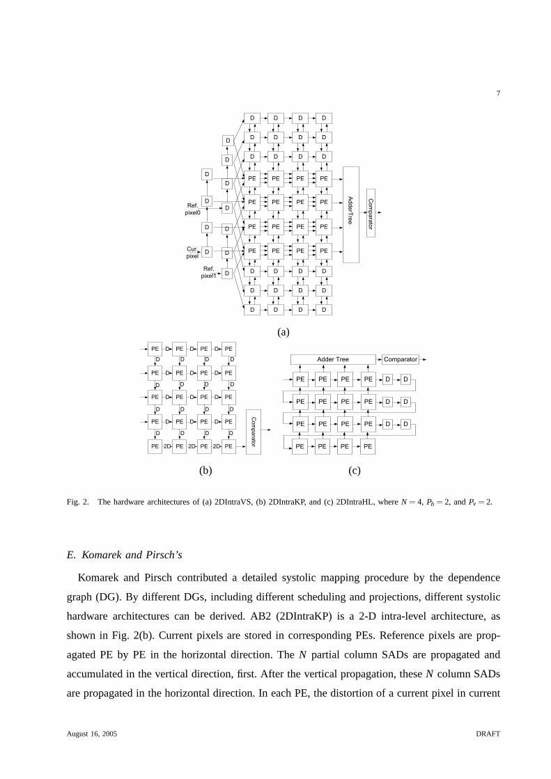
Fig. 2. The hardware architectures of (a) 2DIntraVS, (b) 2DIntraKP, and (c) 2DIntraHL, whereN = 4, Ph = 2, andPv = 2.

E. Komarek and Pirsch’s

Komarek and Pirsch contributed a detailed systolic mappingprocedure by the dependence

graph (DG). By different DGs, including different scheduling and projections, different systolic

hardware architectures can be derived. AB2 (2DIntraKP) is a2-D intra-level architecture, as

shown in Fig. 2(b). Current pixels are stored in corresponding PEs. Reference pixels are prop-

agated PE by PE in the horizontal direction. TheN partial column SADs are propagated and

accumulated in the vertical direction, first. After the vertical propagation, theseN column SADs

are propagated in the horizontal direction. In each PE, the distortion of a current pixel in current


8

MB is computed and added with the partial column SAD which is propagated in PEs from top

to bottom in the vertical direction. In the horizontal propagation, theseN column SADs are

accumulated one by one byN adders and 2N registers.

F. Hsieh and Lin’s

Hsieh and Lin proposed another 2-D intra-level hardware architecture with search range buffer

(2DIntraHL), as shown in Fig. 2(c). 2DIntraHL consists ofN PE arrays in the vertical direction,

and each PE array is composed ofN PEs in a row. In 2DIntraHL, reference pixels are propagated

with propagation registers one by one, which can provide theadvantages of serial data input and

increasing the data reuse. Current pixels are still stored in PEs. TheN partial column SADs are

propagated in the vertical direction from bottom to up. In each computing cycle, each PE array

generatesN distortions of a searching candidate and accumulates thesedistortions withN partial

column SADs in the vertical propagation. After the accumulation in the vertical direction,N

column SADs are accumulated in the top adder tree in one cycle. The longer latency for loading

reference pixels and large propagation registers are the penalties for the reduction of memory

bandwidth and memory bitwidth.

G. Proposed Propagate Partial SAD

We propose a 2-D intra-level architecture,Propagate Partial SAD[18]. Figure 3(a) and

(b) shows the concept and hardware architecture ofPropagate Partial SAD, respectively. The

architecture is composed ofN PE arrays with 1-D adder tree in the vertical direction. Current

pixels are stored in each PE, and two sets ofN continuous reference pixels in a row are

broadcasted toN PE arrays at the same time. In each PE array with 1-D adder tree, N distortions

are computed and summed by 1-D adder tree to generate one row SAD, as shown in Fig. 3(c). The

row SADs are accumulated and propagated with propagation registers in the vertical direction,

as shown the right part of Fig. 3(b).

The detailed data flow ofPropagate Partial SADis shown in Fig. 4. The reference data

of searching candidates in the even and odd columns are inputted by Ref. Pixels 0and Ref.

Pixels 1, respectively. After initial cycles, the SAD of the first searching candidate in the 0th

column is generated, and the SADs of the other searching candidates are sequentially generated

in the following cycles. When computing the lastN−1 searching candidates in each column,


9

��

��

��

��

��

��

��

�� !�"�� !�#��

��

��

��

��

��

��

�

�

�

� �

� �

� �

��

��

��

��

� �

�

��

��

��

� � � �

��

��

(a) (b) (c)

Fig. 3. (a) The concept, (b) the hardware architecture, (c) the detailed architecture of PE array with 1-D adder tree ofPropagate

Partial SADarchitecture, whereN = 4.

��

��

�

�

�

�

�

�

�

�

��

��

��

�� !�"#�$

%��&

%��&

%�� &

%��&

%��&

%��&

%�� &

�

��

��

��

��

��

��

� ��

��

' ��

�(!�)*#�$)�%��&

��(!+�� !+�(��+� ,��,�) ��(!+��-�� !�� -�� !.�)�/�� "

%��&�(!+�(��+� ,�� "�"�!��*+��(!+�0��!�� "�� "��(!+�+)��1) !�� "��

�

�

�

� "�)*#�$)�%��& � ��(!�)*#�$)�%��&

� "�)*#�$)�%��& ��"�)*#�$)�%��& ��(!�)*#�$)�%�� &

� "�)*#�$)�%�� & ��"�)*#�$)�%��& �!+�)*#�$)�%��&�(!�)*#�$)�%��&

� "�)*#�$)�%��& ��"�)*#�$)�%�� & �!+�)*#�$)�%��&�(!�)*#�$)�%��&

� "�)*#�$)�%��& ��"�)*#�$)�%��& �!+�)*#�$)�%�� &�(!�)*#�$)�%��&

� "�)*#�$)�%��& ��"�)*#�$)�%��& �!+�)*#�$)�%��&�(!�)*#�$)�%�� &

� "�)*#�$)�%�� & ��"�)*#�$)�%��& �!+�)*#�$)�%��&�(!�)*#�$)�%��&

� "�)*#�$)�%��& ��"�)*#�$)�%�� & �!+�)*#�$)�%��&�(!�)*#�$)�% ��&

� "�)*#�$)�% ��& ��"�)*#�$)�%��& �!+�)*#�$)�%�� &�(!�)*#�$)�% ��&

Fig. 4. The detailed data flow of the proposedPropagate Partial SADarchitecture, whereN = 4 andPh = Pv = 2.

the reference data of searching candidates in the next columns are started to be inputted through

another reference input. Then the hardware utilization is 100% except the initial latency. In

Propagate Partial SAD, by broadcasting reference pixel rows and propagating partial row SADs

in the vertical direction, it provides the advantages of fewer reference pixel registers and a shorter

critical path.

H. Proposed SAD Tree

Figure 5(a) shows the concept of the proposedSAD Treearchitecture. The proposedSAD Tree

is a 2-D intra-level architecture and consists of a 2-D PE array and one 2-D adder tree with

propagation registers, as shown in Fig. 5(b) and (c). Current pixels are stored in each PE, and

reference pixels are stored in propagation registers for data reuse. In each cycle,N×N current

and reference pixels are inputted to PEs. Simultaneously,N continuous reference pixels in a


10

��

��

��

��

��

��

��

��

� �

��

� �

��

� �

��

� �

��

��

��

� �

�

��

��

��

��

�

�

�

�

�

�

��

��

��

��

��

�

�

��

��

��

�� !

(a) (b) (c)

Fig. 5. (a) The concept, (b) the hardware architecture, (c) the scan order and memory access, of the proposedSAD Tree

architecture, whereN = 4.

row are inputted into propagation registers to update reference pixels. In propagation registers,

reference pixels are propagated in the vertical direction row by row. In SAD Treearchitecture,

all distortions of a searching candidate are generated in the same cycle, and by an adder tree,

N×N distortions are accumulated to derive the SAD in one cycle.

In order to provide a high utilization and data reuse, snake scan is adopted and reconfigurable

data path propagation registers are developed in the proposed SAD Tree, as shown in Fig. 5(c),

which consists of five basic steps from A to E. The first step, A step, fetchesN pixels in a

row and the shift direction of propagation registers is downward. When calculating the lastN

candidates in a column, extra one reference pixel is required to be inputted, that is, B step. When

finishing the computation of one column, the reference pixels in the propagation registers are

shifted left in step C. Because the reference data have already been stored in the propagation

registers, the SAD can be directly calculated. The next two steps, step D and E, are the same as

to step A and B except that the shift direction is upward. After finishing the computation of one

column in the search range, we execute step C and then go back to step A. This procedure will

iterate until all searching candidates in the search range have been calculated. The detailed data

flow is shown in Fig. 6. By snake scan and reconfigurable propagation registers, the data reuse

between two successive searching candidates can be maximized, and the hardware utilization is

approaching 100%.


11

��

� ��

�

�

�

�

�

�

�

�

��

��

��

��

��

��

��

��

��

��

��

��

��

��!��!��!��!��

��"��"��"��"��"!�

��#��#��#��#��#!�

$

��%��&��'�(��%��&��$��%��&)��'�(��&)��*(�&+��

�� %��%��&��&��,��%��-��&�(��'��%��.��(��'

�

�

�

��

��

��

��

��!��!��!��!��

��

�

��

��

��

�

�

��

��

��

�

�

��

��

��

�

�

�

�

�

��/��/��/��/��/!�

��0��0��0��0��0!�

��"��"��"��"��"!�

��#��#��#��#��#!�

��/��/��/��/��/!�

��0��0��0��0��0!�

��

��!��!��!��!��

��"��"��"��"��"!�

��#��#��#��#��#!�

��/��/��/��/��/!�

��/��/��/��/!��

��

��!��!��!��!��

��"��"��"��"��"!�

��#��#��#��#��#!�

��#��#��#��#!��

��

��!��!��!��!��

��"��"��"��"��"!�

��"��"��"��"!��

�

� ��!��!��!��!!��

1 ��!��"�

1 ��!��"�

��0��0��0��0!��

��/��/��/��/!�� #��#��#��#!�� "��"��"��"!�� !��!��!��!!��

��!��"��#��#��#��#!�� "��"��"��"!�� !��!��!��!!��

1 ��!��"�

1 ��!��"�

$

��!��!��!!��!"��

��"��"��"!��""��"#��

�

��!��"��"��"��"��"!�� !��!��!��!!�� !��"�

��!��"��!��!��!��!!�� !��"� ��!��"�

��!��"� ��!��"� ��!��"� ��!��"�

��!��"�� !��"�� !��"�� !��"��

��!��!��!!��!"�� !��"�� !��"�� !��"��

��

��

��

��

��

��

��

��

$�&(�

�

�

�

�

!

"

#

/

0

��

2

��

��

��

��

�!

�"

�#

�/��

Fig. 6. The detailed data flow of the proposedSAD Treearchitecture, whereN = 4 andPh = Pv = 3.

I. The Impact of Variable Block Size Motion Estimation in Hardware Architectures

There are many methods to support VBSME in hardware architectures. For example, we can

increase the number of PEs or the operating frequency to do MEfor different block sizes,

respectively. One of them is to reuse the SADs of the smallestblocks, which are the blocks

partitioned with the smallest block size, to derive the SADsof larger blocks. By this method,

the overhead of supporting VBSME is only the slight increaseof gate count, and the other

factors, such as frequency, hardware utilization, memory usage, and so on, are the same as

those of FBSME. When this method is adopted, the circuit for the SAD calculation is the only

difference between FBSME and VBSME for hardware designs. Hence the impact of supporting

VBSME in hardware architectures is dependent on the different data flows of partial SADs.

In inter-level architectures, the data flow of partial SADs is simple, where the partial SADs

are stored in each PE. In intra-level architectures, there are two kinds of data flows of partial

SADs, propagating with propagation registers or no partialSADs. In the following, the impact

of supporting VBSME with three different data flows is analyzed. We assume that the size of a

MB is N×N, and it can be divided inton×n smallest blocks of size(N/n)×(N/n).

1) Data Flow I–Storing in PEs: In inter-level architectures, each PE is responsible for

computing the distortion and accumulating the SAD of a searching candidate, as shown in

Fig. 7(a). The partial SADs are stored in PEs. When supporting VBSME, the number of partial


12

��

��

��

�

��

��

�

��

� ��

��

(a) (b)

Fig. 7. The hardware architecture of inter-level PE with Data Flow I for (a) FBSME, whereN = 16, (b) VBSME, where

N = 16 andn = 4.

SADs is increased from one ton2. In order to store these partial SADs, more data buffers are

required in each PE, as shown in Fig. 7(b). Besides, there areextra two n2-to-1 and 1-to-n2

multiplexers in each PE for the selection of partial SADs. All PEs of inter-level architectures,

including 1DInterYSW, 2DInterYH, and 2DInterLC, should bereplaced with that in Fig. 7(b) to

support VBSME. The number of bits for the data buffer in each PE is increased fromlog2N2+8

to n2×(log2(N/n)2+8), whereN2 and (N/n)2 are the number of pixels in one block, and 8 is

the wordlength of one pixel. For example, if a MB is 16×16 and can be divided into 16 4×4

blocks, the size of data buffer is increased from 16 bits to 16×12 bits in one PE.

2) Data Flow II–Propagating with Propagation Registers:In intra-level architectures, partial

SADs can be accumulated and propagated with propagation registers. Each PE computes the

distortion of one corresponding current pixel in current MB. By propagation adders and registers,

the partial SAD is accumulated with these distortions. The hardware architecture ofPropagate

Partial SADis a typical example, as shown in Fig. 3(b), where the partialSADs are propagated in

the vertical direction. When supporting VBSME, more propagation registers are required to store

partial SADs of the smallest blocks. In each propagating direction, the number of propagation

registers aren times of that in the original for then smallest blocks in the other direction.

For example, in Fig. 8(a), when supporting VBSME, because there are four smallest blocks in

the horizontal direction, we have to propagate four partialSADs of the smallest blocks in the

vertical direction at the same time in order to reuse them. Therefore, the propagation registers

are duplicated four copies, and the number of propagation registers increases from 16 to 64.


13

��

��

�

�

�

�

��

�

�

�

�

��

�

�

�

�

��

�

�

�

�

��

�� !��"�

�#��$ $�� !��"�

��

��

��

��

��

��

��

�� ! � ��

��

��

(a) (b)

Fig. 8. The hardware architecture for VBSME of (a) the proposed Propagate Partial SADarchitecture with Data Flow II, (b)

the proposedSAD Treearchitecture with Data Flow III, whereN = 16 andn = 4.

Furthermore, some extra delay registers are required in order to synchronize the timing of the

SADs of the smallest blocks, as shown in Fig. 8(a). In each propagating direction, the number of

delay registers is equal ton×(n(n−1)/2)×(N/n). That is, in Fig. 8(a), there are 4 delay register

arrays. In each delay register array, the top smallest blockrequires(4−1)×16/4 delay registers,

the second smallest block requires(4−2)×16/4 delay registers, the third smallest block requires

(4−3)×16/4 delay registers, and the bottom smallest block does not require delay registers.

Totally, there are 4×(4(4−1)/2)×(16/4) delay registers. In addition toPropagate Partial SAD,

2DIntraHL also propagate the partial SADs in the vertical direction, and in 2DIntraKP, the partial

SADs are propagated in two directions. In these three architectures, extra propagation and delay

registers are required in their propagating directions when VBSME is supported.

3) Data Flow III–No Partial SADs:In intra-level architectures, it is possible that no partial

SADs are required to be stored, such asSAD Tree. Each PE computes the distortion of one

current pixel for a searching candidate, and the total SAD isaccumulated by an adder tree in

one cycle, as shown in Fig. 5(a). Because there is no partial SAD in this architecture, there is

no registers overhead to store partial SADs when supportingVBSME. The adder tree is the one

to be reorganized to support VBSME, as shown in Fig. 8(b). That is, we partition the 2-D adder

tree in order to get the SADs of the smallest blocks first, and then based on these SADs, to

derive the SADs of large blocks. Although there is no additional register overhead, the adder

tree additions required to support VBSME do require additional area, such as, 2DIntraVS.


14

III. EXPERIMENTAL RESULTS AND DISCUSSION

In this section, we discuss the performances of the six previous works and our two proposed

hardware architectures,Propagate Partial SADand SAD Tree, in a video coding system with

MB pipelining architectures, where several MBs are processed at the same time but in different

functional modules, such as ME and reconstruction. First ofall, we summarized the charac-

teristics of eight ME hardware architectures in Table I and II. In Table I, the number of PEs,

required cycles, and latency are discussed to show the degree of parallelism and utilization, and

the data flow of partial SADs are listed to categorize the impact of supporting VBSME in each

hardware. In Table II, current buffer, reference buffer, and memory bitwidth are used to evaluate

the tradeoff between data buffer and memory usage. Note thatbecause we reuse the SADs of

the smallest blocks to derive the SADs of larger blocks, the impact of supporting VBSME in

hardware architectures is only the increase of chip area. The other factors are the same for

FBSME and VBSME.

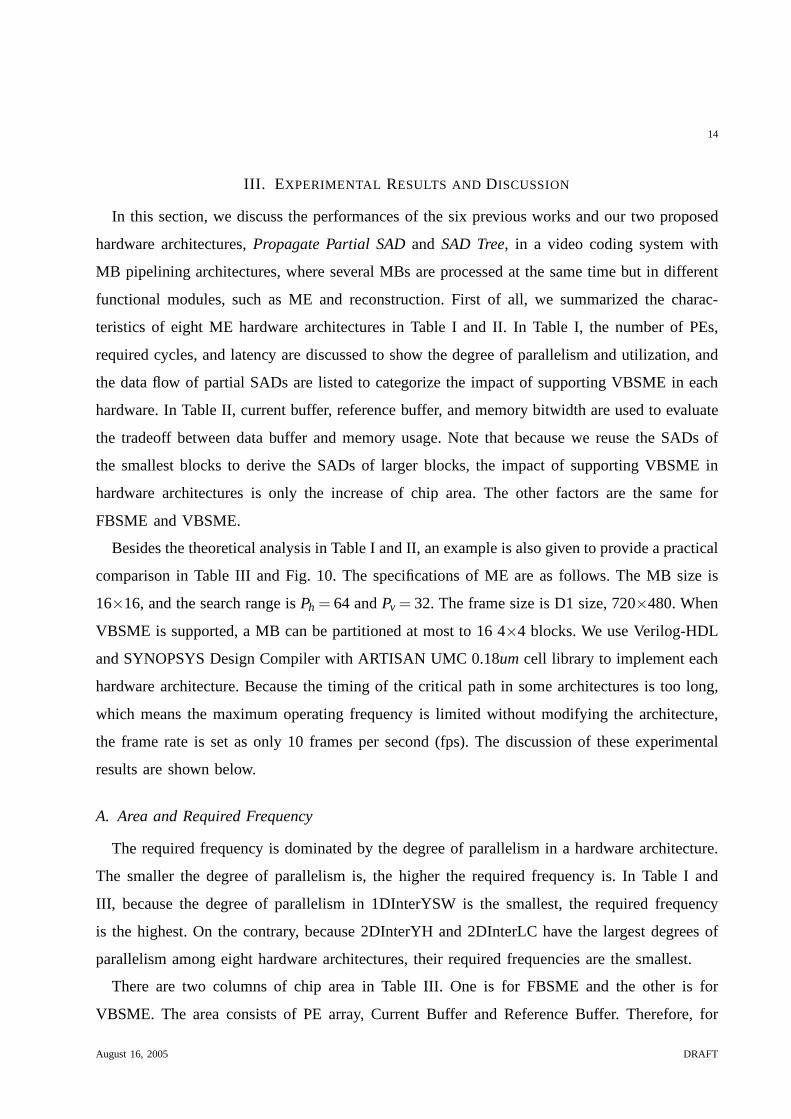
Besides the theoretical analysis in Table I and II, an example is also given to provide a practical

comparison in Table III and Fig. 10. The specifications of ME are as follows. The MB size is

16×16, and the search range isPh = 64 andPv = 32. The frame size is D1 size, 720×480. When

VBSME is supported, a MB can be partitioned at most to 16 4×4 blocks. We use Verilog-HDL

and SYNOPSYS Design Compiler with ARTISAN UMC 0.18umcell library to implement each

hardware architecture. Because the timing of the critical path in some architectures is too long,

which means the maximum operating frequency is limited without modifying the architecture,

the frame rate is set as only 10 frames per second (fps). The discussion of these experimental

results are shown below.

A. Area and Required Frequency

The required frequency is dominated by the degree of parallelism in a hardware architecture.

The smaller the degree of parallelism is, the higher the required frequency is. In Table I and

III, because the degree of parallelism in 1DInterYSW is the smallest, the required frequency

is the highest. On the contrary, because 2DInterYH and 2DInterLC have the largest degrees of

parallelism among eight hardware architectures, their required frequencies are the smallest.

There are two columns of chip area in Table III. One is for FBSME and the other is for

VBSME. The area consists of PE array, Current Buffer and Reference Buffer. Therefore, for


15

TABLE I

THE PARALLELISM , CYCLES, LATENCY, AND DATA FLOW OF EIGHT HARDWARE ARCHITECTURES

Name No. of PEs Operating Cycles Latency Data Flow

(Cycles/Macroblock) (Cycles)

1DInterYSW [5] 2Ph N2×2Pv +2Ph N2 Data Flow I

2DInterYH [7] 2Ph×2Pv 2N2 N2 Data Flow I

2DInterLC [8] 2Ph×2Pv 2N2 2N2 Data Flow I

2DIntraVS [9] N2 2Ph×2Ph +N×2Pv N×2Pv Data Flow III

2DIntraKP [6] N2 2Pv×(N+2Ph)+N 3N Data Flow II

2DIntraHL [10] N2 (2Pv +N−1)×(2Ph +N−1) 2N+(N−1)×(2Ph +N−2) Data Flow II

Propagate Partial SAD N2 2Ph×2Pv +N−1 N Data Flow II

SAD Tree N2 2Ph×2Pv +N−1 N Data Flow III

Note: The analysis is based on a video coding system with macroblock pipelining architecture.

TABLE II

THE DATA BUFFER AND MEMORY BITWIDTH OF EIGHT HARDWARE ARCHITECTURES

Name Current Buffer Reference Buffer Memory Bitwidth

(Pixels) (Pixels) (Bits/Cycle)

1DInterYSW [5] 2Ph−1 - (2Ph/N+2)×8

2DInterYH [7] N2−1 - (2(2Pv/N)×(2Ph/N)+1)×8

2DInterLC [8] - 2Ph×2Pv (2(2Pv/N)×(2Ph/N)+1)×8

2DIntraVS [9] N2 N×(4Pv +N−2) {1,(2)∗}×8

2DIntraKP [6] N2 N×(N−1) N×8

2DIntraHL [10] N2 N2 +(N−1)×(2Ph−2) 1×8

Propagate Partial SAD N2 - {N, (2N)∗}×8

SAD Tree N2 N×(N+1) {N,(N+1)∗}×8

Note: (.)∗ is the worst case.

FBSME, the area of 1DInterYSW is the smallest. The area of 2DInterLC is larger than that of

2DInterYH because of the huge reference buffer, as shown in Table II. Because of the same

reason, the area of 2DIntraVS is also larger than that of proposedSAD Tree. The impact of

supporting VBSME is apparently observed in the other columnof area, the area for VBSME,

in Table III. Among these eight hardware architectures, allinter-level architectures with Data

Flow I increase gate count dramatically. The chip area is fivetimes of that in FBSME at least.


16

In intra-level architectures with Data Flow II, the increase of gate count is much smaller, and

the increasing ratio is from 9.8% to 46.3%. If intra-level architectures have Data Flow III, the

area overheads are 0.2% and 5.8%, for the proposedSAD Treeand 2DIntraVS, respectively.

Due to the characteristics of inter-level architectures, the chip area overhead of inter-level

architectures for VBSME is large. In three inter-level architectures, the overhead of 2DInterLC

is the smallest, because of a lot of propagation registers in2DInterLC compared to other

architectures. The similar condition occurs in the comparison of 2DIntraHL andPropagate

Partial SAD, so the chip area overhead of supporting VBSME in 2DIntraHL is smaller than

that in Propagate Partial SAD. 2DIntraKP has the largest chip area overhead in three intra-level

architectures with Data Flow II, because the partial SADs are propagated in two directions. In

2DIntraVS, although there is no partial SAD to be stored, thepartial SADs are accumulated

by propagation. Then not only the adder tree has to be reorganized, but also extra adders are

required. InSAD Tree, SAD is directly summed by a 2-D adder tree, so the adder tree is only

reorganized without extra adders. Hence the chip area overhead of 2DIntraVS is larger than that

of SAD Tree. Moreover, the chip area overhead ofSAD Treeis also the smallest in the eight

hardware architectures.

B. Latency

The latency is defined as the number of start-up cycles that a hardware takes to generate the first

SAD. The latency is more important for a video coding system than single ME module, because

the latency affects the effect of parallel computation. In avideo coding system, we usually use

a large degree of parallelism to achieve realtime computation. However, if a module has a long

latency and it cannot be shortened by parallel architectures, the effect of parallel computation

is reduced. That is, a shorter latency is better for video coding systems. There are two factors

to affect the latency. One is the type of a hardware architecture. In inter-level architectures, the

latency is at leastN×N, as shown in Table I and III. Conversely, there is no constraint in intra-

level architectures. The other factor to affect the latencyis the memory bitwidth and reference

buffer, as shown in Table II. If there is a large reference buffer but fewer memory bitwidth, for

example, 2DIntraVS or 2DIntraHL, the architecture takes more initial cycles to load reference

data into the reference buffer. Compared to these hardware architectures, the other intra-level

architectures, such as proposedPropagate Partial SADandSAD Tree, have shorter latencies.


17

C. Utilization

In general, inter-level architectures can continuously compute MB by MB, so the initial cycles

can be neglected and the utilization will be 100%. For instance, if the frame-level pipeline

[19] is adopted, the hardware utilization of ME module will be 100%. However, this feature

is not necessary for a video coding system with MB pipeliningarchitectures, because MB

pipelining interrupts the computation of motion estimation. Therefore, we defined the utilization

as Computing cycles / Operating cycles for a MB. Then, the utilization is dominated by the

operating cycles. The operating cycles include three parts, latency, computing cycles, and bubble

cycles. Computation cycles are the number of cycles when we can get one SAD at least. That is,

if the utilization is 100%, we can get one SAD in each cycle at least. Fewer operating cycles will

let the penalty of the latency be apparent. The more bubble cycles are, the lower the utilization

is. 2DInterYH, and 2DInterLC are two examples which have lowutilizations because of their

fewer operating cycles, as shown in Table I and III. In our proposed two hardware architectures,

there are shorter latencies and no bubble cycles, so their utilizations can achieve 99.8%.

D. Memory Usage

Memory usage consists of two parts, memory bitwidth and memory bandwidth. Memory

bitwidth is defined as the number of bits which a hardware has to access from memory in each

cycle, and memory bandwidth is re-defined as the number of bits which a hardware has to

access from memory for a MB. Memory bandwidth affects the loading of system bus without

on-chip memory or the power of on-chip memory, and memory bitwidth is the key to the

data arrangement of on-chip memories. Memory bitwidth and bandwidth are affected by the

data reuse scheme and operating cycles. From Table II, because 2DIntraHL and 2DIntraVS have

larger reference buffers to reuse reference pixels, the required memory bitwidths and bandwidths

are fewer. In 2DInterYH and 2DInterLC, because of their highdegrees of parallelism as shown

in Table I, the large memory bitwidths are required. But the memory bandwidths are much fewer

because of their fewer operating cycles. The data reuse schemes in 2DIntraKP and the proposed

two hardware architectures are similar, and the differences of these three architectures are the

different data reuse schemes when changing columns.


18

TABLE III

THE COMPARISON OFEIGHT HARDWARE ARCHITECTURES FORFBSMEAND VBSME IN SIX CRITERIA

Name Area(FBS) Area(VBS) Freq. Bitwidth Bandwidth LatencyUtil.

(Kgates) (Kgates) (MHz) (Bits/Cycle) (Kbits per MB) (Cycles) (%)

1DInterYSW [5] 61.9 359.6 222.7 80 1,290 256 99.2

2DInterYH [7] 2,907.0 20,422.0 6.9 520 260 256 50.0

2DInterLC [8] 4,055.0 21,647.0 6.9 520 260 512 50.0

2DIntraVS [9] 301.3 318.7 127.7 16 90 1024 88.9

2DIntraKP [6] 108.8 159.1 123.7 128 1,146 48 89.3

2DIntraHL [10] 231.9 254.6 124.4 8 90 2162 72.5

Propagate Partial SAD 66.6 81.5 110.8 256 1,259 16 99.8

SAD Tree 88.4 88.6 110.8 136 1,044 16 99.8

Note: The specification is D1 size, 10 fps, and the search range is [-64, 64) in a video coding system with

macroblock pipelining architecture.

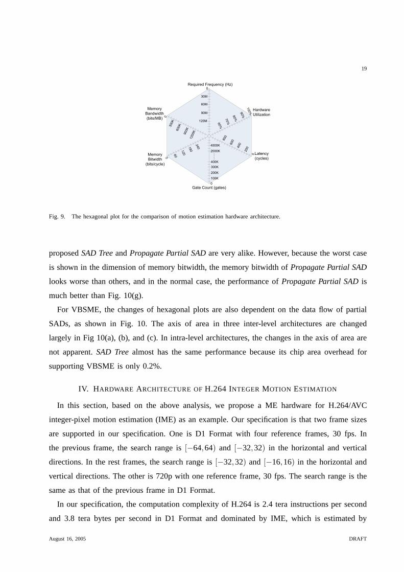
E. Hexagonal Plot

Figure 9 is a hexagonal plot. It is used to visualize the characteristics of ME hardware

architectures. The six design criteria in Table III are shown in the hexagonal plot, in which

the closer the point is to the center, the worse the performance is. Therefore, the advantages and

disadvantages of ME hardware architectures can be observedeasily in a hexagonal plot. Note

that, in various video coding systems or hardware system platforms, the weighting of each axis

will be very different, and we can use these hexagonal plots to select the optimal architecture

based on different constraints for the system integration.

In Fig. 10, there are two lines in one hexagonal plot. One is the solid line for FBSME, and

the other is the dotted line for VBSME. From Fig. 10, we can easily observe the characteristics

of each hardware and see that the similar architectures has similar hexagonal plots and charac-

teristics. 1DInterYSW provides low hardware cost, high utilization, smaller memory bitwidth,

and short latency. The hexagonal plots of 2DInterYH and 2DInterLC are similar because they

are 2-D inter-level architectures with large propagation registers and provide lower required

frequencies and lower memory bandwidths. In addition, 2DIntraHL and 2DIntraVS are 2-D

intra-level architectures with large propagation registers and have good performances in the

memory usages, so their hexagonal plots are also alike. The hexagonal plots of 2DIntraKP,


19

�

�

��

��

��

��

�

��

��

��

��

�

��

��

��

��

�

��

��

��

��

� ��

�� !"�

! ��# ��

$��%�" ��

& ��

�� %��'��

(��#��)

�*��+� �%��

��'��

( ��#��)�

�*��+�(�

��

��

��

��

�

��,

-�,

��,

��,

��,

��

��

……

Fig. 9. The hexagonal plot for the comparison of motion estimation hardware architecture.

proposedSAD TreeandPropagate Partial SADare very alike. However, because the worst case

is shown in the dimension of memory bitwidth, the memory bitwidth of Propagate Partial SAD

looks worse than others, and in the normal case, the performance ofPropagate Partial SADis

much better than Fig. 10(g).

For VBSME, the changes of hexagonal plots are also dependenton the data flow of partial

SADs, as shown in Fig. 10. The axis of area in three inter-level architectures are changed

largely in Fig 10(a), (b), and (c). In intra-level architectures, the changes in the axis of area are

not apparent.SAD Treealmost has the same performance because its chip area overhead for

supporting VBSME is only 0.2%.

IV. HARDWARE ARCHITECTURE OFH.264 INTEGER MOTION ESTIMATION

In this section, based on the above analysis, we propose a ME hardware for H.264/AVC

integer-pixel motion estimation (IME) as an example. Our specification is that two frame sizes

are supported in our specification. One is D1 Format with fourreference frames, 30 fps. In

the previous frame, the search range is[−64,64) and [−32,32) in the horizontal and vertical

directions. In the rest frames, the search range is[−32,32) and [−16,16) in the horizontal and

vertical directions. The other is 720p with one reference frame, 30 fps. The search range is the

same as that of the previous frame in D1 Format.

In our specification, the computation complexity of H.264 is2.4 tera instructions per second

and 3.8 tera bytes per second in D1 Format and dominated by IME, which is estimated by


20

�

�

��

��

��

��

�

��

��

��

��

�

��

��

��

��

�

��

��

��

��

� ��

�� !"�

! ��# ��

$��%�" ��

& ��

�� %��'��

(��#��)

�*��+� �%��

��'��

( ��#��)�

�*��+�(�

��

��

��

��

�

��,

-�,

��,

��,

��,

�./��012

��

��

……

�

�

��

��

��

��

�

��

��

��

��

�

��

��

��

��

�

��

��

��

��

� ��

�� !"�

! ��# ��

$��%�" ��

& ��

�� %��'��

(��#��)

�*��+� �%��

��'��

( ��#��)�

�*��+�(�

��

��

��

��

�

��,

-�,

��,

��,

��,

�./��0!

��

��

……

�

�

��

��

��

��

�

��

��

��

��

��

��

��

��

�

��

��

��

��

� ��

�� !"�

! ��# ��

$��%�" ��

& ��

�� %��'��

(��#��)

�*��+� �%��

��'��

( ��#��)�

�*��+�(�

��

��

��

��

�

��,

-�,

��,

��,

��,

�./��&�

��

��

……

(a) (b) (c)

�

�

��

��

��

��

�

��

��

��

��

�

��

��

��

��

�

��

��

��

��

� ��

�� !"�

! ��# ��

$��%�" ��

& ��

�� %��'��

(��#��)

�*��+� �%��

��'��

( ��#��)�

�*��+�(�

��

��

��

��

�

��,

-�,

��,

��,

��,

�./�� 01

��

��

��

……

�

�

��

��

��

��

�

�

��

��

��

��

��

��

��

��

�

��

��

��

��

� ��

�� !"�

! ��# ��

$��%�" ��

& ��

�� %��'��

(��#��)

�*��+� �%��

��'��

( ��#��)�

�*��+�(�

��

��

��

��

�

��,

-�,

��,

��,

��,

�./�� 0

��

��

……

�

�

��

��

��

��

�

��

��

��

��

�

��

��

��

��

�

��

��

��

��

� ��

�� !"�

! ��# ��

$��%�" ��

& ��

�� %��'��

(��#��)

�*��+� �%��

��'��

( ��#��)�

�*��+�(�

��

��

��

��

�

��,

-�,

��,

��,

��,

�./�� !&

��

��

……

(d) (e) (f)

�

�

��

��

��

��

�

��

��

��

��

��

��

��

��

�

��

��

��

��

� ��

�� !"�

! ��# ��

$��%�" ��

& ��

�� %��'��

(��#��)

�*��+� �%��

��'��

( ��#��)�

�*��+�(�

��

��

��

��

�

��,

-�,

��,

��,

��,

.��/ � ��

. �� %�012

��

��

……

�

�

��

��

��

��

�

��

��

��

��

�

��

��

��

��

�

��

��

��

��

� ��

�� !"�

! ��# ��

$��%�" ��

& ��

�� %��'��

(��#��)

�*��+� �%��

��'��

( ��#��)�

�*��+�(�

��

�

��

��

��

�

��,

-�,

��,

��,

��,

./0�1��

��

��

……

(g) (h)

Fig. 10. Hexagonal plots of eight hardware architectures for fixed block size motion estimation and variable block size motion

estimation. (a) 1DInterYSW. (b) 2DInterYH. (c) 2DInterLC.(d) 2DIntraVS. (e) 2DIntraKP (f) 2DIntraHL. (g)Propagate Partial

SAD. (h) SAD Tree.

instruction profiling of reference software, JM7.3 [20] andthe simulation environment is P4-1.8

GHz and 1 GB memory with Redhat Linux 6.2. In general, the ultra large computation complexity

can be solved by the parallel computation, but the huge external memory bandwidth can not.

Therefore, the huge memory bandwidth is a difficult challenge for hardware design. Besides, there

are two problems. First, because of VBSME and Lagrangian mode decision, the data dependency

of motion vector predictor prohibits from the parallel computation between the smaller blocks

in a MB. Secondly, when the high processing ability is necessary, the hardware cost of ME


21

MB Boundary��

��

��

��

��

��

��

��

MB Boundary

MB Boundary

Predictor for B16x16 = medium(MV0, MV1, MV2)

MV0

MV1 MV2

B16x16� �

� �

��

��

��

��

��

� ��

��

��

��

�� !

��

"��#� ��$��#�

��

��

(a) (b) (c)

Fig. 11. The motion vector predictor for (a) the 4×8 block, (b) the 16×16 block, and (c) the modified motion vector predictor

for all blocks.

hardware architectures with high degrees of parallelism isalso required to be discussed. In

the following subsections, we propose a hardware architecture for H.264/AVC IME to reduce

memory bandwidth and solve the above problems.

A. Hardware Architecture Design

1) Modified Algorithm:First, we divide the computation of ME into two parts, integer-pixel

ME and fractional-pixel ME (FME), and propose two individual hardware accelerators for IME

and FME [21], respectively. This is because the utilizationof hardware accelerators can be

significantly improved by this way, and in this paper, we onlyfocus on the part of IME. Second,

in the original Lagrangian mode decision, the MV predictor of a block is the medium MV

among the MVs of top, top-right, left neighboring 4×4 blocks, as shown in Fig. 11(a) and (b),

but in the parallel computation of hardware architectures,the coding modes of the neighboring

4×4 blocks can not be decided in parallel, especially when the block size is 4×4. Hence the

parallel computation conflicts with Lagrangian mode decision in VBSME. In order to solve this

confliction, we modify the MV prediction of Lagrangian mode decision. The medium among

the MVs of top-right, top, top-left blocks is used instead ofthe original. The modified MV

prediction is shown in Fig. 11(c). By this modification, not only the parallel computation in a

MB becomes feasible, but also the quality is maintained [22].

2) Hardware Architecture with M-parallelism:Based on the analysis in Sec. II and III, our

proposed two hardware architectures have better performances for VBSME and provide a small

chip area and high utilization. We select them to further discuss the impact of parallelism,


22

TABLE IV

THE NUMBER OF REGISTERS INM-Parallel Propagate Partial SADAND M-Parallel SAD Tree

The Number of PEs Propagate Partial SAD SAD Tree

(bits) (bits)

1×256 PEs 3,920 4,224

2×256 PEs 5,792 4,480

4×256 PEs 9,536 4,992

8×256 PEs 17,024 6,016

because a high degree of parallelism is required for our specification. In our specification, we

require eight sets ofPropagate Partial SADor SAD Treeto achieve the realtime computation.

Therefore, eight sets ofPropagate Partial SADandSAD Tree, which can process eight successive

candidates in a row at the same time, are combined asEight-Parallel Propagate Partial SAD

andEight-Parallel SAD Tree, respectively.

When M-Parallel architectures are required, the propagation registers for partial SADs cannot

be shared and they should be duplicated. But if the registersare used to store reference pixels,

the registers can be shared in different PE arrays, and only extra a few registers are required. For

example, inEight-Parallel Propagate Partial SAD, eight sets of propagation registers for partial

SADs are required, but inEight-Parallel SAD Tree, the number of registers for storing reference

pixels is only increased 16 pixels in one row. Then the increasing ratio is only(16−1+16)/16,

not 8. Table IV shows the number of required registers in these two architectures with different

degrees of parallelism. The increasing ratio ofM-parallel Propagate Partial SADis much larger

than that ofM-parallel SAD Tree. HenceSAD Treeis much more suitable for high resolution

or large computation complexity. AlthoughPropagate Partial SADhas no advantages of a high

degree of parallelism, for low resolution or small computation complexity,Propagate Partial

SADstill has a similar performance and shorter critical path compared toSAD Tree.

3) Applied Techniques for Hardware Cost Reduction:Due to a high degree of parallelism, the

required chip area is huge even if the proposedSAD Treehas the smallest chip area. We adopt

several techniques to reduce the hardware cost and memory bandwidth. The first is subsample

[23]. The pattern of subsample is interleaved and similar tothe pattern of the chess. The second

method is the pixel truncation [24]. We only preserve five bitprecision for all current and


23

reference pixels. Figure 12(a) shows the modifiedSAD Treewith subsample and pixel truncation

and variable block size adder tree (VBS Adder Tree), which isused to reuse the SADs of

the smallest blocks to derive the SADs of larger blocks. The shared reference buffer ofEight-

Parallel SAD Treenot only can provide the required reference pixels for eightsets of SAD

Tree, as shown in Fig. 12(b), but also save the on-chip memorybandwidth. Moving window is

also adopted to save the computation complexity and reduce on-chip memory bandwidth. The

search range is partitioned into four regions,[−64,15], [−48,31], [−32,47], and [−16,63] in

the horizontal direction. According to MV predictor, one offour regions is selected and the

searching candidates in this region are computed. Besides,Level C Search Area Reuse [25] [26]

and on-chip frame boundary padding are applied to reduce theoff-chip memory bandwidth.

4) Hardware Architecture of IME:Figure 12(c) shows the whole architecture of H.264 IME.

IME Controller controls the actions of all submodules.On-Chip Paddingis responsible for the

extension of a frame boundary.Upper Ref. & MV SRAMand RefMV Bufferare used to store

MVs of the top MB row to generate MV predictor. MV cost in Lagrangian mode decision is

calculated inMV Cost Gen.. Routeris used to reorder the order of the data which are read from

Luma Ref. Pels SRAMs. Ref. Pels Arrayis the data buffer for storing reference pixels to reuse

reference pixels and reduce the memory access.41-Parallel Eight-Input Comparator Arrayis

responsible for finding optimal 41 MVs which have the smallest cost for different block size.

B. Experimental and Implementation Results

1) Experimental and Implementation Results:Figure 13(a) and (b) show the comparisons of

RD curves between JM7.3 and our proposed motion vector prediction. We have tested many

sequences from QCIF to HDTV, and two of them are Racecar (720×288, 30fps) and Taxi

(672×288, 30fps). At high bit rate, which is larger than 1 Mbps, thequality loss is near zero,

and at low bit rate, the quality is degraded 0.1 dB. The results of pixel truncation are shown in

Fig. 13(c). Based on the simulation results, the degradation of five bit precision is little, but that

of four bit precision is from 0.1 dB to 0.2 dB. Finally, the RD curve of our encoder chip is shown

in Fig. 13(d). The test sequences are Crouching Tiger HiddenDragon and Crew. The former

is D1 Format, and the latter is HDTV Format. The coding performance of our encoder chip is

competitive with that of JM7.3. Moreover, because we also refine the Lagrangian multiplier, our

performance is better than that of the original at very high bitrate.


24

��

��

��

�� !�

��"#"��

$�� !�

"��

��

��

��

��

��

��

��…

��

��

�� !��"��

"��#��$

��$�%��!��"�&�&��"�!��

��$�%��!��!�&��"�!��

��$�%��!��&��"�!��

(a) (b)

��

��

��

��

��

��

��

��

��

� �� !�� "#��$��

��

��

%��"#��$�&"� $��

��

��

��

��!�"��#�� "�

�$��"�� % ��

��"�%�

%�&�

��##�

��'��#��

��"�!�'�#��

%� �� (�� )��"*

&'�� "�� "�

��#

��+��)�&

��

�

�

�

�

�

(c)

Fig. 12. The hardware architecture of H.264 integer motion estimation. (a) The architecture of SAD Tree with subsample and

truncation and VBS Adder Tree. (b) Share reference buffer with reconfigurable data paths and data sharing. (c) The overview

of H.264 integer motion estimation.

In the hardware implementation, our specification is statedin the beginning of Sec. IV. In

SDTV, the block size can be from 16×16 to 4×4. In HDTV, although our proposed IME

architecture can support all kinds of block sizes, we only support the block modes which block

sizes are larger than or equal to 8×8 due to the limit of FME [22]. Verilog-HDL and SYNOPSYS

Design Compiler with ARTISAN UMC 0.18um cell library are used to design the hardware.

BecauseSAD Treecan support VBSME with less overhead and many techniques forthe reduction

of hardware cost are applied, the total gate count of H.264/AVC IME is only 330.2K gates, and

the operating frequency is 81 MHz at SDTV or 108 MHz at HDTV. The on-chip memory size

is 208 Kbits.


25

Racecar

25

26

27

28

29

30

31

32

33

34

35

300 800 1300 1800 2300 2800 3300Bit Rate (Kbps)

PS

NR

(dB

)

JM

Proposed MVP for mode decision

Taxi

29

30

31

32

33

34

35

36

37

38

39

40

41

42

300 800 1300 1800 2300 2800 3300Bit Rate (Kbps)

PS

NR

(dB

)

JM

Proposed MVP for mode decision

(a) (b)Racecar

25

26

27

28

29

30

31

32

33

34

35

300 800 1300 1800 2300 2800 3300

Bit Rate (Kbps)

PS

NR

(dB

)

JM

7 bits precision

6 bits precision

5 bits precision

4 bits precision

Rate Distortion Curves

37

38

39

40

41

42

43

44

45

46

47

48

0 5 10 15 20 25 30 35 40Bit-Rate (Mbps)

PS

NR

(dB

)

Crew (HDTV 720p) by JM7.3

Crew (HDTV 720p) by Ours

Crouching Tiger Hidden Dragon (D1) by JM7.3

Crouching Tiger Hidden Dragon (D1) by Ours

(c) (d)

Fig. 13. The comparison of RD curves between JM7.3 and our proposed encoder. (a) The comparison of modified motion

vector prediction in Racecar. (b) The comparison of modifiedmotion vector prediction in Taxi. (c) The comparison of pixel

truncation in Racecar. (d) The comparison of our proposed encoder.

2) Memory Bandwidth:Figure 14 shows the required off-chip and on-chip memory bandwidth

of four reference frames in our D1 specification. In Fig. 14, five data reuse schemes are discussed,

and the related data are theoretical value, not the simulated results. The first data reuse scheme

is the simplest one. There is only one RISC in the hardware without any cache. Because of no

on-chip memories as the search area cache, reference pixelsare inputted directly from off-

chip memories and no on-chip memory bandwidth is required. The second scheme is one

RISC with Search Area Cache. By use of the on-chip memory, 866.6 Mbytes/s of the off-

chip memory bandwidth is required, but the on-chip memory bandwidth is increased to 138.4

Gbytes/s. However, this tradeoff is worth because the access of off-chip memories takes much

more power and cycles than those of on-chip memories, in general. The third data reuse scheme


26

��

��

��

��

��

��

�� !

��

��"�#�

�$%&��'(�)��*�+,!%-��.�--'%/

�� !

��

��0'/��&.�� "�#�

��

�$%&��'(�)��*�+,!%-��.�--'%/

�� !

��

��0'/��&.�� "�#�

��,�'%/�1'%-,2

��3�

�*,��+�%-2'-��

$44&��'(��*,��+�%-2'-��

$%&��'(��*,��+�%-2'-��

��5�#��%'6!��,!��,44&��'(�**,��

��5�#��%'6!��,!��,%&��'(�**,��

Fig. 14. The memory reduction of H.264 IME.

is the second one with Level C Search Area Reuse, and then the off-chip memory bandwidth can

be reduced again. So only 152.2 Mbytes/s of the off-chip memory bandwidth is necessary. On

the other hand, because of the data reuse inSAD Tree, the on-chip memory bandwidth is only

8.9 Gbyte/s. In the fourth data reuse scheme, on-chip frame boundary padding is adopted, so

the off-chip memory bandwidth is reduced again. As for on-chip memory bandwidth, byEight-

Parallel SAD Tree, 1.8 Gbytes/s of the on-chip memory bandwidth is required. Finally, because

the moving widow is applied in the fifth data reuse scheme, theon-chip memory bandwidth is

reduced to 1.4 Gbytes/s.

In summary, we saved 99.9% off-chip memory bandwidth compared to the data reuse scheme

of RISC. Compared to the general data reuse scheme, Level C Search Area Reuse, the off-chip

memory bandwidth is reduced to 89.6%. Furthermore, 99.22% on-chip memory bandwidth is

saved by our proposedEight-Parallel SAD Treeand moving window.

V. CONCLUSION

In this paper, we not only propose two hardware architectures but also analyze the impact of

supporting VBSME in hardware architectures. Base on our analysis, the impact of supporting

VBSME is dependent on the data flow of partial SADs in a hardware architecture. In general

cases, inter-level architectures have large penalties when supporting VBSME, because the number

of registers and hardware circuits for calculating partialSADs in VBSME are increased largely. In


27

intra-level architectures, there are two cases. If the partial SADs are propagated and accumulated,

extra propagation and delay registers are required. If there is no partial SAD in intra-level

architectures, the chip area overhead of supporting VBSME is less than others. Moreover, we

also utilize a hexagonal plot to show the characteristics ofa hardware architecture. By the

hexagonal plots, the advantages and disadvantages of each hardware architecture are shown

apparently. Therefore, based on different system constraints, we can easily select the optimal

architecture by use of the hexagonal plots.

Our proposed hardware architectures,Propagate Partial SADand SAD Tree, can support

FBSME as well as VBSME.Propagate Partial SADhas the advantages of fewer reference

pixel registers and a shorter critical path by broadcastingreference pixel row and propagating

partial SADs.SAD Treeutilizes a 2-D PE array with one adder tree and the reconfigurable

reference buffer, which can maximize the data reuse betweensuccessive searching candidates.

Our proposed two hardware architectures can provide low cost, high utilization and less area

overhead when supporting VBSME compared to six previous approaches. Moreover,Propagate

Partial SADis suitable for the low resolution or small search range, andSAD Treehas advantages

when high degree of parallelism is required.

In the last part of this paper, a hardware architecture for H.264/AVC IME is also proposed.

A modified algorithm is proposed to solve the data dependencyof motion vector prediction in

Lagrange mode decision. Pixel truncation, subsample, and moving window are applied to reduce

the hardware cost. By the proposedEight-Parallel SAD Tree, on-chip memory with Level C

Search Area Reuse, and On-Chip Frame Boundary Padding, the most critical issue of H.264/AVC

IME, large memory bandwidth, is solved. 99.9% off-chip memory bandwidth and 99.22% on-

chip memory bandwidth are significantly reduced. We use Verilog-HDL and SYNOPSYS Design

Compiler with ARTISAN UMC 0.18um cell library to implement the hardware. The total gate

count of this design is 330.2 K, and the on-chip memory size is208 Kbits. The design can

achieve full frame rate for D1 Format with four reference frames at 81 MHz and for a 720p

stream with one reference frame at 108 MHz.

REFERENCES

[1] Video Coding for Low Bit Rate Communication, ITU-T Recommendation H.263 version 3, Feb. 1998.

[2] Information Technology - Coding of Audio-Visual Objects - Part 2: Visual, ISO/IEC 14496-2, 1999.


28

[3] Sridhar Srinivasan, John Hsu, Tom Holcomb, Kunal Mukerjee, Shanker L. Regunathan, Bruce Lin, Jie Liang, Ming-

Chieh Lee, and Jordi Ribas-Corbera, “Windows Media Video 9:overview and application,”Signal Processing: Image

Communication, vol. 19, pp. 851–875, Sept. 2004.

[4] Joint Video Team, “Draft ITU-T recommendation and final draft international standard of joint video specification,”May

2003.

[5] K. M. Yang, M. T. Sun, and L. Wu, “A family of VLSI designs for the motion compensation block-matching algorithm,”

IEEE Trans. Circuits Syst., vol. 36, no. 10, pp. 1317–1325, Oct. 1989.

[6] T. Komarek and P. Pirsch, “Array architectures for blockmatching algorithms,”IEEE Trans. Circuits Syst., vol. 36, no.

10, pp. 1301–1308, Oct. 1989.

[7] H. Yeo and Y. H. Hu, “A novel modular systolic array architecture for full-search block matching motion estimation,”

IEEE Trans. Circuits Syst. Video Technol., vol. 5, no. 5, pp. 407–416, Oct. 1995.

[8] Y. K. Lai and L. G. Chen, “A data-interlacing architecture with two-dimensional data-reuse for full-search block-matching

algorithm,” IEEE Trans. Circuits Syst. Video Technol., vol. 8, no. 2, pp. 124–127, Apr. 1998.

[9] L. De Vos and M. Stegherr, “Parameterizable VLSI architectures for the full-search block-matching algorithm,”IEEE

Trans. Circuits Syst., vol. 36, no. 10, pp. 1309–1316, Oct. 1989.

[10] C. H. Hsieh and T. P. Lin, “VLSI architecture for block-matching motion estimation algorithm,”IEEE Trans. Circuits

Syst. Video Technol., vol. 2, no. 2, pp. 169–175, June 1992.

[11] J. F. Shen, T. C. Wang, and L. G. Chen, “A novel low-power full search block-matching motion estimation design for

H.263+,” IEEE Trans. Circuits Syst. Video Technol., vol. 11, no. 7, pp. 890–897, July 2001.

[12] N. Roma and L. Sousa, “Efficient and configurable full-search block-matching processors,”IEEE Trans. Circuits Syst.

Video Technol., vol. 12, no. 12, pp. 1160–1167, Dec. 2002.

[13] V. L. Do and K. Y. Yun, “A low-power VLSI architecture forfull-search block-matching motion estimation,”IEEE Trans.

Circuits Syst. Video Technol., vol. 8, no. 4, pp. 393–398, Aug. 1998.

[14] X. Q. Gao, C. J. Duanmu, and C. R. Zou, “A multilevel successive elimination algorithm for block matching motion

estimation,” IEEE Trans. Image Processing, vol. 9, no. 3, pp. 501–504, Mar. 2000.

[15] M. Brunig and W. Niehsen, “Fast full-search block matching,”IEEE Trans. Circuits Syst. Video Technol., vol. 11, no. 2,

pp. 241–247, Feb. 2001.

[16] S. F. Chang, J. H. Hwang, and C. W. Jen, “Scalable array architecture design for full search block matching,”IEEE Trans.

Circuits Syst. Video Technol., vol. 5, no. 4, pp. 332–343, Aug. 1995.

[17] H. M. Jong, L. G. Chen, and T. D. Chiueh, “Parallel architectures for 3-step hierarchical search block-matching algorithm,”

IEEE Trans. Circuits Syst. Video Technol., vol. 4, no. 4, pp. 407–416, Aug. 1994.

[18] Y. W. Huang, T. C. Wang, B. Y. Hsieh, and L. G. Chen, “Hardware architecture design for variable block size motion

estimation in MPEG-4 AVC/JVT/ITU-T H.264,” inProc. of IEEE Int. Symp. Circuits Syst. (ISCAS’03), 2003, pp. 796–799.

[19] S. Kittitornkun and Y. H. Hu, “Frame-level pipelined motion estimation array processor,”IEEE Trans. Circuits Syst. Video

Technol., vol. 11, no. 2, pp. 248–251, Feb. 2001.

[20] Joint Video Team Reference Software JM7.3, http://bs.hhi.de/ suehring/tml/download/, Aug. 2003.

[21] T.-C. Chen, Y.-W. Huang, and L.-G. Chen, “Analysis and design of macroblock pipelining for H.264/AVC VLSI

architecture,” inProc. of IEEE Int. Symp. Circuits Syst. (ISCAS’04), 2004, pp. 273–276.

[22] Y. W. Huang, T. C. Chen, C. H. Tsai, C. Y. Chen, T. W. Chen, C. S. Chen, C. F. Shen, S. Y. Ma, T. C. Wang, B. Y. Hsieh,


29

H. C. Fang, and L. G. Chen, “A 1.3tops H.264/AVC signle-chip encoder for HDTV applications,” inProc. of IEEE Int.

Solid-State Circuits Conf. (ISSCC’05), 2005, pp. 128–129.

[23] T. Koga, K. Iinuma, A. Hirano, Y. Iijima, and T. Ishiguro, “Motion compensated interframe coding for video conferencing,”

in Proc. Nat. Telecommun. Conf. (New Orleans, LA), 1981, pp. G5.3.1–5.3.5.

[24] Zhongli He and M.-I. Liou, “Reducing hardware complexity of motion estimation algorithms using truncated pixels,” in

Proc. of IEEE Int. Symp. Circuits Syst. (ISCAS’97), 1997, pp. 2809–2812.

[25] J. C. Tuan, T. S. Chang, and C. W. Jen, “On the data reuse and memory bandwidth analysis for full-search block-matching

VLSI architecture,” IEEE Trans. Circuits Syst. Video Technol., vol. 12, no. 1, pp. 61–72, Jan. 2002.

[26] Mei-Yun Hsu, Scalable module-based architecture for MPEG-4 BMA motion estimation, Master Thesis, National Taiwan

Univ., June 2000.


30

L IST OF FIGURES

1 The hardware architectures of (a) 1DInterYSW, (b) 2DInterYH, and (c) 2DInterLC,

whereN = 4, Ph = 2, andPv = 2. . . . . . . . . . . . . . . . . . . . . . . . . . . . . 6

2 The hardware architectures of (a) 2DIntraVS, (b) 2DIntraKP, and (c) 2DIntraHL,

whereN = 4, Ph = 2, andPv = 2. . . . . . . . . . . . . . . . . . . . . . . . . . . . . 7

3 (a) The concept, (b) the hardware architecture, (c) the detailed architecture of PE

array with 1-D adder tree ofPropagate Partial SADarchitecture, whereN = 4. . . 9

4 The detailed data flow of the proposedPropagate Partial SADarchitecture, where

N = 4 andPh = Pv = 2. . . . . . . . . . . . . . . . . . . . . . . . . . . . . . . . . . 9

5 (a) The concept, (b) the hardware architecture, (c) the scan order and memory

access, of the proposedSAD Treearchitecture, whereN = 4. . . . . . . . . . . . . 10

6 The detailed data flow of the proposedSAD Treearchitecture, whereN = 4 and

Ph = Pv = 3. . . . . . . . . . . . . . . . . . . . . . . . . . . . . . . . . . . . . . . . 11

7 The hardware architecture of inter-level PE with Data FlowI for (a) FBSME, where

N = 16, (b) VBSME, whereN = 16 andn = 4. . . . . . . . . . . . . . . . . . . . 12

8 The hardware architecture for VBSME of (a) the proposedPropagate Partial SAD

architecture with Data Flow II, (b) the proposedSAD Treearchitecture with Data

Flow III, where N = 16 andn = 4. . . . . . . . . . . . . . . . . . . . . . . . . . . 13

9 The hexagonal plot for the comparison of motion estimationhardware architecture. 19

10 Hexagonal plots of eight hardware architectures for fixedblock size motion estima-

tion and variable block size motion estimation. (a) 1DInterYSW. (b) 2DInterYH.

(c) 2DInterLC. (d) 2DIntraVS. (e) 2DIntraKP (f) 2DIntraHL.(g) Propagate Partial

SAD. (h) SAD Tree. . . . . . . . . . . . . . . . . . . . . . . . . . . . . . . . . . . . 20

11 The motion vector predictor for (a) the 4×8 block, (b) the 16×16 block, and (c)

the modified motion vector predictor for all blocks. . . . . . . .. . . . . . . . . . . 21

12 The hardware architecture of H.264 integer motion estimation. (a) The architecture

of SAD Tree with subsample and truncation and VBS Adder Tree.(b) Share

reference buffer with reconfigurable data paths and data sharing. (c) The overview

of H.264 integer motion estimation. . . . . . . . . . . . . . . . . . . . .. . . . . . 24


31

13 The comparison of RD curves between JM7.3 and our proposedencoder. (a) The

comparison of modified motion vector prediction in Racecar.(b) The comparison of

modified motion vector prediction in Taxi. (c) The comparison of pixel truncation

in Racecar. (d) The comparison of our proposed encoder. . . . .. . . . . . . . . . 25

14 The memory reduction of H.264 IME. . . . . . . . . . . . . . . . . . . . .. . . . . 26

L IST OF TABLES

I The Parallelism, Cycles, Latency, and Data Flow of Eight Hardware Architectures . 15

II The Data Buffer and Memory Bitwidth of Eight Hardware Architectures . . . . . . 15

III The Comparison of Eight Hardware Architectures for FBSME and VBSME in Six

Criteria . . . . . . . . . . . . . . . . . . . . . . . . . . . . . . . . . . . . . . . . . . 18

IV The Number of Registers inM-Parallel Propagate Partial SADandM-Parallel SAD

Tree . . . . . . . . . . . . . . . . . . . . . . . . . . . . . . . . . . . . . . . . . . . 22


0 analysis and architecture design of variable block...

Documents