0

I),

ARMC Report No. 4.76-1

S,

ANALYSIS OF DUCTED PROPELLERS IN STEADY FLOW

R. Van Houten

February, 1986

DTIC- ELECTE

~,JUL 0 1986

-.- B -

AIRFLOW RESEARCH AND MANUFACTURING CORP.

jp1m ed i-*i public TeIeose"I, ' Dt,,,UtbU~l e-') Urii1 t - , .d"

86 .,

86-

AIRFLOW RESEARCH AND MANUFACTURING CORP.i' 304 Pleasant Street

* Watertown, MA 02172(617) 926-3061Telex 294129 ARMC UR

ARMC Report No. 4.76-1

ANALYSIS OF DUCTED PROPELLERS IN STEADY FLOW

R. Van Houten

February, 1986

Copyright (c) Airflow Research and Manufacturing Corporationand Massachusetts Institute of Technology, 1986.

This research was carried out under subcontract GC-A-483454 fromMassachusetts Institute of Technology (MIT OSP 94409)

in support of contract N00014-84-K-0072 under theNaval Sea Systems Command

General Hydromechanics Research (GHR) Programadministered by the

David W. Taylor Naval Ship Research and Development Center

APPROVED FOR PUBLIC RELEASEDISTRIBUTION UNLIMITED JUL33 1986

E3 .,. .

VB

-UN1CASSIFIED

kECuU'TY %.LASSiFICATIONi Of THItS IlluE AVAj 1"k ~REPORT DOCUMENTATION PAGE

isa REPORT SECURITY CLASSIFICATION lb RESTRICTIVE MARKINGSWNC.ASSWME N/A

2a SECUR-ITY CLASSIFICATIO01 AUTHORITY I DISTRIBUITION IAVAIL.MILITY Of REPORTN N/A A2P1P:77D FOR PUBLIC RELEASE,

2b OECLASSIFICATION iDOWNGRADING SCHEDULE DIs7Rxm37raN tL~rDD

4 PERFORMING ORGANIZATIO REPORT NUMBER(S) S MONITORING ORGANIZATION REPORT NUMBER($)

(he NAME OF PERFORMING ORtGANJZATION 6b OFFICE SYMBOL 7a NAME OF MONITORING ORGANIZATIONAirflow Research & (of omliablei DAVID W. 7RYLCSR NAVAL SHIP REERC NManufacturing Corp. DWLM CE Co, 1504 (1505)

6C ADDRE SS (Colty. Stare. OW ZIP Cd) 7b ADDRESS (Coty. Uate. and lI, COWe)

*304 Pleasant St. BMSA MAD20450W a t e r t o w n , M A 0 2 1 7 2 g o O F C Y B O R C R M E T I S R N D E T F C I O 2 0U M-5 0 0

&a NAME OF FUNDING /SPONSORINGSbOICSYBL POREETISRMNIETICTONUMRI-ORGANIZATION (fsp~o

Naval Sea Systems Camiand SE 05R24 Conitract Number - N00014-84-K-00726C DAES (City'. State. dnd ZIP Code) 10 OURE FUNDING NUMBERS

wPROGRAMI PROJECT TASK WORK UNITWashingon, D. C. 20360 ELEMENT NO NO NO0 ACCESSION NO

/8________________________________61153N SR 023 01 123454 N/AJ, 11 TITLE (JAIiclua Security Clasuification)

ANALYSIS OF DUCTED PROPELLERS IN STEADY FLOW- (Unclassified)

*12 PFRSONAL AUTHOR(S)R. Van Houten

* 13a TYPE OF REPORT 1 3b TIME COVERED IsI DATE OF REPORT (Yea Month Day) l' AgICOUNTFinal FROM 1 / 8 4 To 2/86 I February 11986 J bi

'6 SjP. EVFENTARY NOTATION Sponsored unider the Naval Sea Systems Cmnand General HydramechanicsRe-search (GHR) Program adninistered by the David W. Taylor Naval Ship R&D Center, Code

I? COSATI CODES is SUBJECT TERMS IContinue an rverse if necessary and identify by block number)

-FELD GROUP sue-GROUP GM. Program, Propellers, Ducted Propellers, Tip Gap,200 Banded Propellers, Lifting Surface Theory, Vortex

'I~ABVACT(Cntiue ~ ~ Lattice.19 AS'ACT Coninu on evese f ncesaryand edent~fy by block nurnber)

- This report describes a computer, program (DPSF); based on lifting surfacetheory, which- analyzes the hydrodynamic performance of a ducted or banded

Ipropeller in an axisymmetric inflow. Special attention is given themodelling of flow through the clearance gap. Calculated results are comparedwitn experimental data, and numerical convergence is demonstrated. -

20 DS'R-B..AON 'AVAILABILITY 0$ ASSTRAC' 121 ABSTRACT SECURITY CLASSIFICATION

JPUNCLASSIfIEDUNLIMiTED 0 SAME AS OPT 0 DTIC USERS I tRC)aMIFIEDk . o [jF AE ,q~j~i NDIVDUAL22b TELEPHONE WcIlude AreaCodr) 22c OFFICE SYMBOL

~MEJD ~A4 aDVDL 202-227-1503 Code 1504/1505

DO FORM 1473. e4 MAR 33 APR edition may bef used unil estmiusted SECURITY CLASSIFICATION OF THIS PAGEAll other edition% are obsolete UN1LASSWFIE

11. P

- ..-- ~ - ....- . *.* .*-.... *% * . N 1-.-

TABLE OF CONTENTS

1. BACKGROUND. 1

2. VISCOUS EFFECTS IN TIP GAP FLOWS. 4

3. LIFTING LINE REPRESENTATIONS OF FLOWSWITH TIP GAPS. 12

4. VORTEX LATTICE REPRESENTATION OF FLOWS* WITH TIP GAPS. 25

5. THE DUCTED PROPELLER ANALYSIS PROGRAM. 29Blade Geometry 30Duct Geometry 32Vortex Lattice 32Wake Geometry 38Wake Alignment 39Source Strength 40Solution of Boundary Value Problem 40Force Calculation 41Results 42Computation Time 54

6. CONCLUSIONS AND RECOMMENDATIONS. 55

7. REFERENCES. 58

* APPENDIX A - MAGNITUDE OF THE GAP BOUNDARYLAYER THICKNESS. 60

*.

it: '

S1. BACKGROUND

It has been known for some time that by operating a

marine propeller in a duct (also called a shroud or nozzle),

certain advantages can be obtained over an open propeller.

When the duct is designed to accelerate the fluid through

the propeller disk, the advantages include an increased

ideal efficiency at a given propeller diameter, an

efficiency curve which is fairly flat over a wide range of

advance ratios, and high bollard pull. The disadvantages of

the ducted propeller are that there is additional viscous

drag on the duct surface, and cavitation can be a problem in

the clearance gap between the blade tips and the duct. A

P propulsor which avoids the latter problem is the banded, or

ring, propeller. In this configuration the shroud is

attached to the blade tips, and rotates with the propeller.

Viscous drag on the band contributes to shaft torque,

resulting in a loss of efficiency, but high tip loading on

the blades can be better maintained in the absence of a tip

gap, and a concentrated tip vortex can be avoided in favor

of a distributed vortex sheei: in the wake of the band. This

may result in delayed cavitation inception relative to an

open propeller.

-4,-0

.4°

.. ......... . ......- .. . .. . ...-... . -.......-- '. .. - -.t v4 ".%%.. -'. - -;-.-" ".-. -.

Ducted and banded propellers have been fitted mainly to

ships operating at low speeds, with heavy disk loading, and

particularly those which must operate at the zero speed

condition, such as tugs and trawlers. However, recent

attention has focused on these configurations for higher

speed naval applications. In order to evaluate the

suitability of ducted and banded propellers for these new

applications, design and analysis methods must be developed

for them.

A first step in this direction was taken when an

analysis program for banded propellers was developed by Van

Houten (1983) under the sponsorship of NSRDC. This program,

called BPSF (Banded Propeller in Steady Flow), was an

..- extension of PSF, a lifting surface analysis program for

open propellers (Greeley, 1982; Greeley and Kerwin, 1982).

In BPSF the radius of the band and its section

characteristics (camber, thickness, and angle of attack)

were allowed to vary circumferentially, the only restriction

being that the axial extent of the band be equal to that of

the tip of the blade. The objective of the work presented

here was to develop an equivalent program for the analysis

of ducted propellers.

-2-

,:-7

* This program, called DPSF, allows there to be an

arbitrary tip gap between the propeller tip and the surface

of the duct. The duct is constrained to be axisymmetric,

* but is allowed to extend axially well beyond the blade tip.

This report presents some of the theory behind this program,

and some representative results. Little effort will be made

* to recap the development of PSF and BPSF, for which the

reader is referred to the beforementioned publications.

6

*-3-

2. VISCOUS EFFECTS IN TIP GAP FLOWS

One of the fundamental problems to be faced in

developing an analysis program for ducted propellers is the

question of accurately modeling the clearance gap between

- - the blade tip and the duct surface. This gap is typically a

fraction of a percent of the propeller diameter, and the

question arises as to the importance of viscous effects in

determining the leakage flow. This question has been

addressed in the past by several investigators, who have

concluded in general that the leakage flow is largely

inviscid in nature. This is supported by some simpie

scaling arguments outlined in Appendix A. Furthermore, the

leakage volume flow rate is to a large extent independent of

the chordwise flow. As a result simple two dimensional

experiments can be used to investigate the flow in the

clearance gap.

Such experiments have been carried out in the past by

Shalnev (1954) , Gearhart (1966) , Booth, Dodge and Hepworth

(1981), and Wadia and Booth (1981). The type of leakage

flow they have found, in the case of a blade tip with a

square cross-section, is shown in figure 2.1. The sharp

corner at the entrance to the gap causes a separation bubble

which then reattaches to the blade tip. The jet at the exit

from the gap causes the rolling up of a vortex on the

suction side of the blade. The presence of the separation

O-4-

7j, S. ~ - 5 ' ~ '. .. ~~5 5 % . . 5.

4.

hSEPARATION

BUBBLE

VORTEX

PRESSURE BLADE SUCTIONSIDE TIP SIDE

Figure 2.1 Observed flow past squareblade tip.

rINFLOWVELOCITY

PRESSURE BLADE SUCTION

SIDE TIP SIDE

Iv

Fiaure 2.2 Inflow velocity distributiondue to duct boundary layer.

.

A. . ., .,. . - < .,,. - , .< ,,.. , ,," ,..--". ,' ' , -.. , .'.. < ... ,.. - - . .-.- . - . .• .. ,. , - . ,

bubble causes the total flow through the gap to be less than

would otherwise be predicted. The reduction in flow is

often given in terms of a discharge coefficient, defined as:

QCQ =V2ATT h

where Q = total volume flow through the gap

Ap = pressure difference across the gap

p = fluid density

h = clearance height

This coefficient is a strong function of blade tip shape.

In the interest of reducing the pressure reduction which

takes place at the gap entrance, and thereby delaying the

onset of gap cavitation, the pressure side of the blade tip

is often rounded off. This can eliminate flow separation in

the gap, and results in an increse in C Q In this respect

the goals of efficiency and good cavitation performance

operate at cross purposes.

C is also a function of the boundary layer on theQ

surface of the duct. This boundary layer causes the

relative inflow velocity vector to twist suddenly, becoming

tangential at the duct surface. When this velocity vector'..1 is decomposed into chordwise and normal components, both

components exhibit boundary layer characteristics. The

normal velocity field, when viewed relative to the blade

-6-

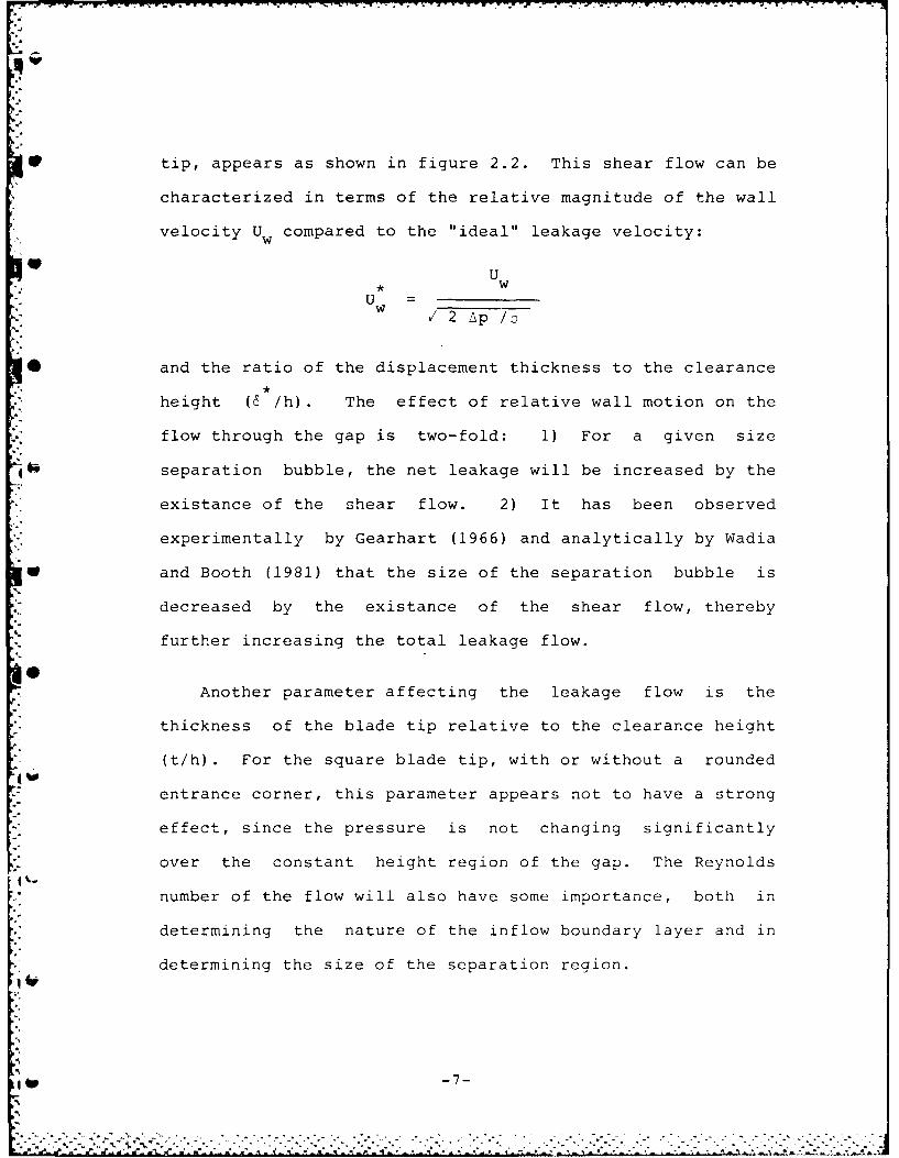
* Btip, appears as shown in figure 2.2. This shear flow can be

characterized in terms of the relative magnitude of the wall

velocity U compared to the "ideal" leakage velocity:0w

,PUU

U w2 Ap /Q

* and the ratio of the displacement thickness to the clearance

height (6 /h). The effect of relative wall motion on the

flow through the gap is two-fold: 1) For a given size

separation bubble, the net leakage will be increased by the

existance of the shear flow. 2) It has been observed

experimentally by Gearhart (1966) and analytically by Wadia

* gand Booth (1981) that the size of the separation bubble is

decreased by the existance of the shear flow, thereby

further increasing the total leakage flow.

oAnother parameter affecting the leakage flow is the

thickness of the blade tip relative to the clearance height

(t/h). For the square blade tip, with or without a rounded

entrance corner, this parameter appears not to have a strong

effect, since the pressure is not changing significantly

over the constant height region of the gap. The Reynolds

number of the flow will also have some importance, both in

determining the nature of the inflow boundary layer and in

determining the size of the separation region.

4W -7-

't t- -

*, .. .- . .

Addressing for the sake of simplicity the cases of a

square blade tip, with and without a rounded leading edge,

with Uw =0, table 2.1 gives the values for C found byQ

various investigators. Although the data is limited, it

indicates that C is relatively independent of both t/h andQ

Reynolds number.

Of the investigators mentioned above, only Gearhart

(1966) and Wadia and Booth (1981) investigated the effect of

wall motion on the leakage flow. Wadia and Booth did so

using a numerical model and considered only the case of a

turbine, where the shear velocities oppose those due to the

pressure gradient. Gearhart investigated a range of values

of Uw but presented C values for 6 /h = .20 only. Thesew Q

are shown in figure 2.3. It can be seen that the curves

approach one another at the higher values of Uw indicating

. that the separated zone on the square blade tip may be

eliminated under these conditions. The numerical results of

Wadia and Booth for a square tip at U =-1 is also shown,w

although they do not indicate the displacement thickness of

the boundary layer assumed. More data on the effect of wall

motion, and in particular the effect of boundary layer

thickness, would be very useful.

6!

- . -8-

Reynolds

Author Number t/h C

6 Square Tip:

Shalnev 15000- 5-30 .762-.838110000

Gearhart 270000 14 .82

Wadia, 6500 6.3 .851Booth

Booth, 2800 3.8-7.5 .80-.82Dodge,Hepworth

Rounded Entrance:

• Shalnev 39000- 5-10 .884-.975115000

Gearhart 270000 14 .92

Table 2.1 Summary of experimental data on dischargecoefficient for 2-D tip gap, with no wall motion.

-9-

1.4

1.4-

CQROUNDED

1.0 ENTRANCE)-

,~1.0-

SQUARE TIP

.8-

-1 0 *12

Uw

Figure 2.3 Effect of wall motion on discharge coefficient.

-10

The application of data such as that shown in figure 2.3

to a global propeller analysis method is straightforward.

It can be presumed that due to the very large mismatch in

length scales between the clearance gap and the other

propeller dimensions, the major impact of the clearance gap

on the global flow field is the resulting leakage flow

* volume. Since C Q represents the reduction in leakage volume

due to viscous effects, these effects can be incorporated in

the global flow field by using for analysis purposes an

"inviscid" clearance gap height h i equal to the product of

C and the physical gap height h:

*g hi = C-hQQ

4h-

1W- -11-

3. LIFTING LINE REPRESENTATIONS OF FLOWS WITH TIP GAPS

The mismatch in length scales between the tip clearance

height and the other relevant propeller dimensions makes

difficult the development of a lifting surface theory for

ducted propellers. In order to describe the small scale tip

clearance region accurately one would normally have to use a

vortex lattice whose spacing is small compared to the gap

size, at least in the tip region. The total number of

control points would be very large and the cost of running

the program correspondingly high. In order to avoid this

expense, a different approach was taken -- namely to

determine if there is an optimum position of the outermost

chordwise vortex on the blade such that numerical

convergence can be accelerated. In order to find such an

optimum, some numerical experiments were carried out using

lifting line theory, with the supposition that the optimum

spanwise arrangement of trailing vortices would not be

affected by the chordwise arrangement of bound vorticies.

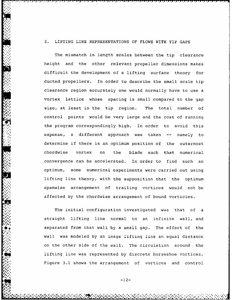
The initial configuration investigated was that of a

straight lifting line normal to an infinite wall, and

separated from that wall by a small gap. The effect of the

wall was modeled by an image lifting line an equal distance

on the other side of the wall. The circulation around the

lifting line was represented by discrete horseshoe vortices.

Figure 3.1 shows the arrangement of vortices and control

-12-

-e ,,.

'.4

4.

*4 As~j L..BOUND (CONTROL IVORTEX POINT24

* /TRAILINGVORTEX

Figure 3.1 Lifting line representation of foilin presence of infinite wall linear spacinq.

4,'

.00

0-0

",.UND CONTROL

VORTEX POINT

*LTRAILILNG,'." VORTEX

Figure 3.2 Liftinq line representation of foilin presence of infinite wall -- cosine spacina.

-13-

",-. . . .. . .. . ...-. : . . . . . .. . . , , - . " . . . . . . . . .. .. .,

points in the case of equally spaced trailers (linear

spacing). The outermost trailers are inset from the tips of

the foil by a fraction of the trailer spacing Is. At the

foil tip furthest from the wall, this inset fraction is

taken to be .25. This is the inset normally used in the

case of an isolated foil, and is analogous to the vortex

position in 2-D vortex lattice theory (James, 1972). The

optimum inset fraction "i" on the end near the wall is

presumably not equal to .25, but approaches that value as

the gap becomes large. For arbitrarily small gaps, the

inset must approach zero, since in that case one would want

to reproduce the results of a single foil of twice the

aspect ratio. The problem can therefore be reduced to that

- of finding how the optimum inset fraction varies from zero

".j- to .25 as the gap varies from zero to infinity.

An alternative lifting line representation uses "cosine"

spacing, with the discrete vortices and control points at

equally spaced values of the Glauert angle 0 as shown in

figure 3.2. The inset fraction is defined as a fraction of

the angular spacing IS of the vortices. On the free end

this inset fraction is taken to be .5. This corresponds to

common practice for isolated airfoils (Lan, 1974). At the

end near the wall, the optimum inset fraction "i" must vary

from zero to .5 as the gap is varied from zero to infinity.

"4

-14-

:-I-

* In order to determine the optimum insets, numerical

experiments were carried out. These experiments were

performed on a foil with optimum loading, in the sense that

* induced drag is a minimum for a given lift. The "exact"

circulation distribution was found for this case by using a

large number of vortices (up to 400) with cosine spacing,

* and requiring the downwash to be a constant at all control

points. The solution was then repeated, using a small

number of vortices, and the inset was varied until a

0% solution was obtained with the smallest mean-squared error

between the calculated vortex strengths and the "exact"

solution at the corresponding control points.

The results of these calculations are shown in figures

3.3 through 3.7. Figure 3.3 shows the calculated "exact"

solution for an isolated foil (infinite gap) and gaps of .1,

.01, .001, and .0001 of the span. In addition, the

solutions are shown using optimum insets and linear spacing

for 5, 10, and 20 vortices. It is clear that the use of an

optimum inset results in a solution which is very close to

the exact one, even when using very few vortices. Figure

3.4 shows comparable results for cosine spacing.

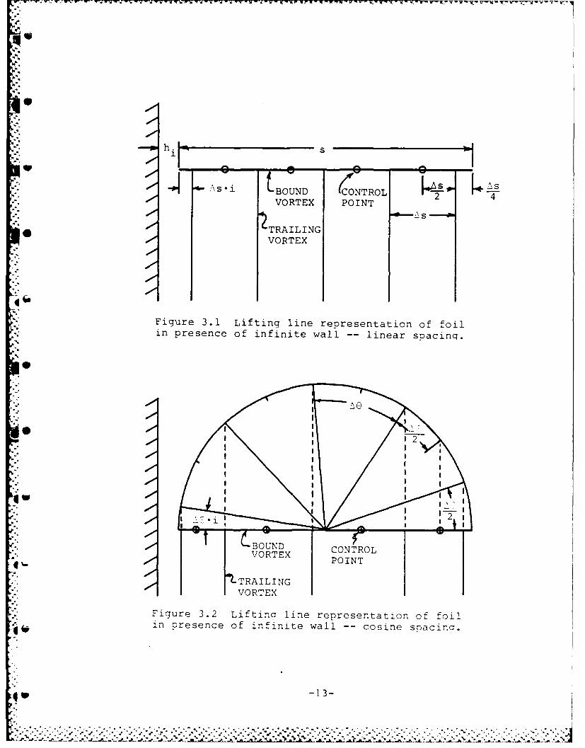
Figures 3.5 and 3.6 show the log of the optimum vortex

inset fraction "i" plotted against the log of the ratio of

.r gap width to the width of the last panel on the foil. It

can be seen that when plotted in this way all the optimum

6P -15-

• . .° ....,o.,. o . ...-, -'-".- t ? . . '. . -'° "'- , - '."-. ,, - . < " '? .-fog° '..

4 4-J 4J )

#1-

t70

-4

0-.0 04

0-4-4-44

m1a021 0 00

I -4 4J-

00

-4 r-4 -44-

CD Lr) - 4-

o -, U) 0 d-

0 0 U

CD *-4 4J

r - -41 41f

00I0

0-.4

r-

Sl.1

00

H~ 4JJ 0JC

S0 0 -d

100o m 01 i-4(U- -H 4J4J .1

m- 0 U)c~

Od 04- 040 1E 0

-4~.

*H~ *H r-* "42

0 0J

0 000 0 U -4

00W 0 (nr22 "-4 (

Q000) 0 0 0

o -1 i 4C(N U) U) 0

0+ 00 40

0 (t(-4 >41i

00O )

-) r-4 0f-4 r-4

II U( 41

0 WO

-. 6 4

log -.8insetfraction"" 9 .30 (g/p)*178 if g/p < .359

-1.0 .250 if g/p a .359

where g = gap

-1.1 /p = panel size

-1.2-4 -3 -2 -1 0 1

log (g/p)

Figure 3.5 Optimum inset fraction, infinite wall, linear soacing.

-.2

-.3

log -.4insetfraction = .64 (g/p) if g/p e .128"i -. 5 -

i = .50 if g/p .128

-. 6

-. 7 I I 4-4 -3 -2 -1 0 1

log (g/p)

*iaure 3.6 Optimum inset fraction, infit wall, cosine snacina.

-18-

!, * - .* . *

(a 0E U)4I --4

00

41 -A--- 4

41~4

* 4 W -.-

~-4 ~lU)

tfL -z x 4-4'4

-~U)

-- i a) CLE441 U) MdH-

a)

I4 4 J

4H U H

4-4~l

H - I--

4U) Q)--4 -H U

00

+ 44-

41 0

insets fall close to a single line, an approximate

expression for which is given in the respective figures. In

the large gap ratio region the expression deviates somewhat

from the calculated optimum, but the solution is quite

insensitive to inset at these gap ratios. At the lower gap

ratios, the solution is much more sensitive, as can be seen

in figure 3.7, where the optimum linear 10 vortex solution

is shown for a gap of .001 span (optimum inset ratio =

.142), as well as the 10 vortex solution using the isolated

airfoil inset fraction of .25. In this case, the incorrect

inset results in an error in induced drag of 10.2%.

The second numerical experiment concerned a wing

separated by a small gap from a perpendicular, symmetrical,

winglet of equal span. This winglet can be thought of as

representing the duct surface in the case of a ducted

propeller. The lifting line representation of this

arrangement using linear spacing is shown in figure 3.8.

The panelling of the main foil is the same as that used in

the case of a foil near a wall. Each half of the winglet is

panelled using the infinite gap inset at the free end and

zero inset at the winglet's midspan position. The number of

panels on the winglet was selected so that the distance from

the center trailing vortex to the nearest control point

matched as nearly as possible the distance between the last

trailer and control point on the main foil. The "exact"

° .- . .. -20-

.........

%

MATCH THESE LENGTHS CONTROL POINT

TRAILING VORTEX

S&

w -

h. S

S

4. LFigure 3.8 Winglet lifting line aeometry, linear spacing.

-21-

-' "---'" < '""" "- "'- -i-'-- <> > -.i, ',.. ...', ..--< "-' -',i.''<i .'. .,- ., i" '/ -'" 2"j" "

L .

minimum drag solution was found by using a large number of

vortices and requiring the downwash on the foil to be a

constant, and the sidewash on the winglet to be zero. The

calculation was then repeated using fewer vortices, and

varying the inset until the solution agreed most closely

with the "exact" one. Figure 3.9 shows as an example the

case of a gap of .001 span, and the optimum solution using

6, 10, and 20 vortices on each foil. The optimum inset

fractions for linear and cosine spacing are given in figures

3.10 and 3.11. These values were used in the ducted

"4 propeller program.

I-2

""- -22-!!::............. ...--................

- V - V

4 4-4 CO

'4-4 OWQ

41

0 4JU

4 -U)

0 0~~U) U) 41r 4C

w )) ):30U) Q 4 J

0) .1 0

U) 0 U ) 4 J -QC)

C) C) 0 0- 0a

~~~~U fo 1i )0U ~- ~ H M

---- >) 4 1 (

~ C X -40

(1 .411Q

1

0 -

0 -

r-4 4J-

toC -23

-. 5

-.6

log -. 7 -insetfraction"il -.. 3 614"i" -. 8 -g/p) if g/p £ .0801

= .250 if g/p m .0801-.9

g gap p = panel size

-1.0 I I I I I

-4 -3 -2 -1 0 1

log (g/p)

Figure 3.10 Optimum inset fraction for winglet with gap,

linear spacing.

-.2

-.3.

log -.4 = .676 (g/p) if q/p < .0209insetfraction i .500 if g/p Z .0209

i" -. 5

-. 6 I I I I-4 -3 -2 -1 0 1

log (g/p)

Figure 3.11 Optimum inset fraction for winglet with gap,cosine spacinq.

-24-

,-. ^0"

4. VORTEX LATTICE REPRESENTATION OF FLOWS WITH TIP GAPS

In order to investigate the applicability of the optimum

insets to non-optimally loaded fails, a planar lifting

surface program was used to analyze a rectangular flat plate

at an angle of attack, placed normal to an infinite wall

from which it is separated by a gap. The insets used wereS

those found optimum for a lifting line normal to an infinite

wall. Cosine spacing (Lan, 1974) was used in the chordwise

direction, and either cosine or linear spacing was used in

the spanwise direction. The drag was calculated using Lan's

method of deriving the suction force from the total upwash

at the leading edge. The effective aspect ratio was then

defined as

c2

A = Le CD

Figures 4.1 and 4.2 show results for a geometric aspect

ratio of 3 and a gap-to-span ratio of .001. The number of

spanwise panels NS was varied from 3 to 24 while the ratio

between the number of spanwise panels to the number of

chordwise panels NC was kept constant, and equal to 3. It

can be seen that the convergence was quite good for both

linear and cosine spacing. Also shown are the corresponding

results obtained using a vortex inset fixed at the infinite

0gap value. It can be seen that while the cosine spacing

results converged quickly for this gap regardless of the

-25-

co iespacing op i u necosine spacing

3.75

dCL

< da

3.50 csn

linear spacing infinite gap inset

3.25 I i1 5 10 15 20 25

NS

Figure 4.1 Convergence of lift curve slope, rectangularwing normal to infinite wall. Aspect ratio = 3.Gap/span = .001. NS/NC = 3.

5cosine spacing/,loine spacing I optimum inset

4.50

Ae ~cosine spacing iniiega ne

linear spacingnse

4.25

4.00

I I I I III

1 5 10 15 20 25NS

Figure 4.2 Convergence of effective aspect ratio,rectangular wing normal to infinite wall. Aspectratio = 3. Gap/span = .001. NS/NC = 3.

-26-

- inset, the convergence of the linear spacing results

improved significantly when the optimum inset was used.

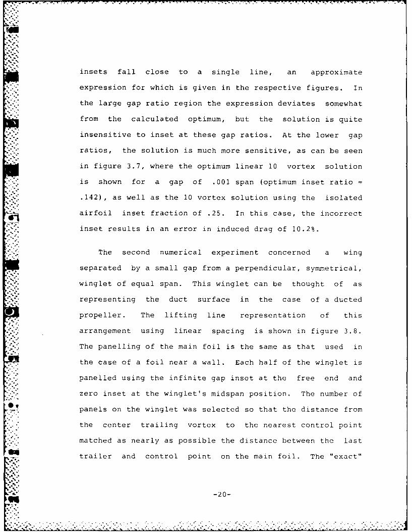
Figure 4.3 shows the calculated increase in the

effective aspect ratio as the gap size is decreased, along

with corresponding results for an optimally loaded foil from

the lifting line calculation, and from a conformal mapping

solution reported by Durand (1963). Surprisingly, this

relationship appears to be practically identical for the two

loading situations. Also shown are the experimental results

of Munk and Cario (1917), as reported by Hoerner (1965),

which indicate that the effect of the gap between two foils

of aspect ratio 3 is significantly less than that predicted

by lifting surface theory. This data is plotted assuming

that C Q= 1. Hoerner gives the Reynolds number, based on

chord length, as 80,000, but gives no thickness data. The

scaling arguments presented in Appendix A indicate that even

for quite thick airfoils, the flow through the gap should be

essentially inviscid for gap/span ratios as large as .01.

The discrepancy between the calculated and measured effect

of a small gap seems too large to be accounted for by

deviations of C from unity. Other experimental dataU

presented by Hoerner and Borst (1975) and by Kerwin, Mandel,

and Lewis (1972) deal with a control surface normal to a

plane. These data also indicate that small gaps have a

smaller effect than theory predicts.

-27-

F-7

. ....

800

60PercentriseinAe

40

20 0Lifting surface theory.- Lifting line theory

+ Durand result

o Experimental data0 " I

-5 -4 -3 -2 -1 0

log Cspan J,:::.:. log I. -n -

Figure 4.3 Percent rise in effective aspect ratio as foilapproaches infinite wall. Comparison of lifting surface theoryfor rectangular foil of aspect ratio 3 with lifting line theoryand results of Durand (1963) for optimally loaded foil.Experimental data from Hoerner (1965).

-.28*. * -. Jjw2-" i >'

5. THE DUCTED PROPELLER ANALYSIS PROGRAM

i, The Ducted Propeller in Steady Flow (DPSF) program is an

adaptation of PSF, developed by Greeley (1982) and described

by Greeley and Kerwin (1982). DPSF analyses ducted and

banded propellers operating in an axisymmetric inflow

consisting of axial, radial, and tangential components.

• This inflow field is generally taken to be the

* circumferential average velocity field at the propeller

plane, and can include the effects of stators and multiple

rotors. The presence of the propeller hub and any other

boundaries to the flow is not modeled. The blade and duct

-' boundary layers are assumed to be thin, so that the flow can

be considered inviscid, except for the empirical addition of

frictional drag.

The blades and duct are represented by straight-line

vortex and source lattice elements of constant strength that

are distributed over the mean camber surface. The trailing

vorticity in the wake of the propeller is represented by

straight-line vortex elements distributed over a specified

surface. The vortices are arranged in horseshoe vortices so

as to satisfy Kelvin's condition, and the strength of the

horseshoe vortices is determined by solving a set of

simultaneous equations, each satisfying the flow tangency

condition at a control point. Source strength is determined

stripwise using a linearized boundary condition.

i4W -29-

[ °. ........

The position of the trailing vortex wake is determined

iteratively by first solving the boundary value problem with

a guessed position, and then aligning the wake with the

computed velocity field. The boundary value problem is then

Sre-solved and the procedure is repeated until convergence is

obtained. When a converged solution is obtained, blade

forces are found by application of the Kutta-Joukowski and

Lagally theorems.

Blade Geometry

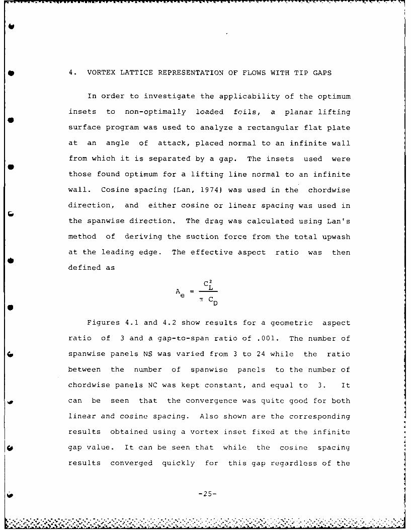
The description of blade geometry in DPSF is as shown

in figure 5.1. The coordinates of the midchord line are

defined by the radial distribution of skew angle ®m (r) and

rake xm(r). The pitch angle '.(r) and chord c(r) define the

angle and extent of the sectional nose-tail line along the

surface of a cylinder of constant radius r. The camber

f(r,s) and thickness t(r,s) describe the section

characteristics of the blade as a function of radius, r, and

the fraction of chord from the leading edge, s. The camber

is measured along the cylindrical surface at right angles to

the nose-tail line. The thickness is measured normal to the

mean line. The propeller radius, R, is defined as the

maximum radius of the blade midchord line.

-30-

wy

Sx

SS

s==O

Figure 5.2 Ducte geometry.

S-31

All geometric properties describing the blade must be

defined out to a radius equal to the largest radial extent

of the blade surface, which is likely to exceed that of the

midchord line . This avoids the uncertainty involved in

extrapolation.

Duct Geometry

The duct (or band) is assumed to be axisymmetric and is

-~ defined in terms of its chord c, chord fraction forward of

the blade tip midchord line "a", angle of attack cc, camber

f(s), and thickness t(s). The gap g between the blade tip

and the inner surface of the duct is assumed to be constant,

* . and may be zero, as in the case of a banded propeller.

Unlike BPSF (Van Houten, 1983) , all quantities are defined

in the (r,x) plane, as shown in figure 5.2. Note that duct

camber is applied in the radial direction only.

Vortex Lattice

The vortex lattice representing the propeller geometry

consists of spanwise and chordwise vortices. The lattice

representing the blade is located on the blade camber

surface. That representing the duct follows the duct camber

surface, but is displaced radially inward so that its

-32-

I - - -W - -rw w -w - - - " • - -€ . • % . . •

distance from the blade tip is equal to the physical tip

gap. A typical vortex lattice is shown in figuure 5.3.

The spanwise spacing of the chordwise vortices on the

blade and duct can be independently selected to be either

linear, cosine, or in the case of the duct, a mixture of the

two. With linear spacing the intersection of the blade

chordwise vortices with the midchord line is given by:

r (R - r H )(m -. 75) +1.. r = "Rr)m.S + rH m =1, 2,...M+1

M+ .25 +i

where rH is the hub radius and M is the number of spanwise

panels. The inset fraction i is given in figure 3.10, where

the panel size is equal to r -r .M+1 M

In the case of cosine spacing, the corresponding

relationship is:

r = .5 (1 - cos (r)) (R-rH) + rH

(m- .5) - m =1,2,...M+I

m (M+ . 5 +i)

where the inset fraction is given in figure 3.11.

The radial position of each chordwise vortex varies as

it crosses the blade. The outermost chordwise vortex

follows the duct camber line. The other chordwise vortices

have a radial variation which is attenuated by the factor

% -33-

-.. "- *-

* .. Figure 5.3 Vortex lattice for NSMB Ka4-55propeller in Nozzle 19.

-34

li (rm rH) /(R-rH)

The spanwise position of control points depends on the

type of spacing used. With linear spacing, the control

points are located midway between chordwise vortices. With

cosine spacing the ith control point is located at a

position corresponding to a value of midway between r. and

ri+l"

One of the duct's chordwise vortices is always located

along the blade tip, displaced radially outward by the gap.

The extension of this vortex beyond the blade leading edge

follows the slope of the blade camber surface at the leading

edge. The extension beyond the blade trailing edge follows

the current wake geometry. The other chordwise vortices on

the duct are displaced circumferentially from this vortex by

0 an amount m which depends on the spacing used. With linearm

spacing,

- (m-1) 27,m = m= ,2 ,...Md +1

Md Z

where Md is the number of spanwise panels on each duct

segment, and Z is the number of blades. With cosine

spacing,

-35-

lI~.::i,: ... :., .-...-...........-...-.............................-. ".".".......... .:":: !..':J :-- :""::

em (1-cos m) / Z

m =1,2,...M d +1

m (m-i) r/Md

With mixed spacing:

2 /Z [b (m_- +.5(l-b) (1-cos( e ))]m Md m

where b can vary between 0 (cosine spacing) and 1 (linear

spacing). The spanwise position of control points follows

that used on the blades.

The spacing method used and the number of panels used on

the blade and duct must be chosen carefully. It is

recomnmended that the distance between the last blade control

point and the last blade chordwise vortex match as closely

as possible the distance between the duct chordwise vortex

at the blade tip and the nearest duct control point.

The spanwise vortices on the blade are located at

- -. "constant values of s, the variable which varies from 0 to 1

along the chord. The chordwise spacing of these vortices

can be selected to be linear:

S = (n- .75)/N n =1,2,...N.'%" n

I -3?6-

*15 %

or cosine:

s = .5 (1-cos (sn))n nn 1,2,...N

s = T (n- .5) /N

where N is the number of panels chordwise. With linear

spacing the ith control point is located midway between the

ith and (i+l)th spanwise vortex. In the case of cosine

spacing the ith control point is located at the value of s

corresponding to a value of s midway between si and S

Spanwise vortices are located on the duct at the same

axial locations as the end points of the spanwise vortices

on the blade. In addition, the portions of the duct

extending beyond the blade leading and trailing edges are

represented by spanwise vortices spaced using the same

41 scheme (linear or cosine) as the blade and central portion

of the duct. A minor exception to this is that when using

cosine spacing the trailing portion of the duct is panelled

"half-cosine", where:

-.(n-.5)n (2N +.5)

= (1-cos(Sn))

The spacing scheme and the panel numbers used should be

selected so that the panel size varies smoothly between the

mid-portion of the duct and the portion extending beyond the

-37-

blade leading and trailing edges. In the case of linear

spacing, the number of panels on the different portions of

the duct should be proportional to their respective axial

extent. In the case of cosine spacing, there are control

points on the duct at the axial position of the blade tip

leading and trailing edges. These control points should be

as nearly as possible midway between the adjacent spanwise

vortices.

In DPSF, all blades (and all segments of the duct) are

panelled identically. This causes run times to be somewhat

longer than if the "non-key" blades were panelled more

coarsely, but the code is significantly simplified.

Wake Geometry

The geometry of the blade transition and ultimate wakes

in DPSF is similar to that in PSF, as described by Greeley

and Kerwin (1982). One difference is that the transition

wake is "grown" by increments in x, rather than e Those

wake points forward of the duct trailing edge are located at

values of x corresponding to the spanwise vortices on the

duct. Behind the duct trailing edge, the wake is grown by

an axial increment which is specified by the user. The

radial location of the blade trailing vortices aft of the

duct trailing edge follows PSF. Forward of the duct

-38-

.4

* trailing edge the radius of the mth trailer is contracted by

an amount equal to (rm-rH)/(R-rH) times the contraction of

the duct camber line between the blade trailing edge and the

* axial position of the wake point in question. The duct

transition wake is modeled by a set of trailing vortices

which begin where the duct chordwise vortices intersect the

*trailing edge of the duct, and parallel the outermost

trailing vortex from the key blade, displaced by the same

angle as that of the chordwise vortex on the duct. The

ultimate wake is modeled the same as in PSF.

* Wake Alignment

The blade transition wake is aligned the same way as in

PSF, except for the case of the outermost blade trailing

vortex. In PSF, the velocity calculated on this vortex

includes a self-induced velocity due to the curvature of the

rolled-up tip vortex. Since in the case of a ducted

propeller the roll-up of the tip vortex is impeded by the

presence of the duct, DPSF does not include this term. The

velocity induced at a segment of the outermost blade

trailing vortex due to itself and the adjacent segments of7 duct chordwise and spanwise vortices is calculated by

assuming that the vorticity in these segments is spread out

over the local duct panel. The magnitude of the local

-39-

,JEW

velocity is just one half the resulting vortex density.

Because the duct chordwise vortices aft of the blade

trailing edge are aligned with the blade transition wake,

this portion of the duct must be repanelled after each

iteration of wake alignment.

Source Strength

As in PSF, the blade thickness is represented by line

sources at the same location as the spanwise vortices.

Their strength is obtained by using thin wing theory, based

on the undisturbed inflow velocity. This undisturbed inflow

velocity is calculated at the mean radius of the source

element at the midchord position. The strength of the line

sources on the duct are calculated in the same way as those

on the blade.

Solution of Boundary Value Problem

The solution of the boundary value problem in DPSF

follows the procedure in PSF exactly. The number of

additional unknowns representing bound vorticity on the duct

is exactly equal to the number of additional equations to be

solved in order to enforce flow tangency on the duct control

-40-

.. . ..o. . . . . . j.

V points.

*O Force Calculation

The calculation of forces in DPSF is practically the

same as that in PSF. The total velocity is calculated at

the midpoint of each singularity, and the Kutta-Joukowski

and Lagally theorems applied. The only exception to this is

that the Lagally forces on the sources due to the

undisturbed relative inflow is not included. This is

necessary in order that the Coriolis force on the fluid

emitted by the sources does not contribute to shaft torque

(Van Houten, 1983).

The forces on the individual singularities are summed up

to give overall forces and moments on each spanwise panel.

The force associated with each spanwise panel on the blade

and duct includes the forces on the spanwise singularities

in that panel and one half the forces on the chordwise

vortices on the edge of the panel. The forces on the

innermost and outermost panels include the entire forces on

the innermost and outermost chordwise vortex, respectively.

These panel forces are then summed to give the forces on the

blade, the duct, and the complete propeller. The torque

exerted on the duct can be included in the propeller torque

or not, depending on whether it in fact represents a duct or

-41-

*7 7 -7 77P

a band.

The empirical viscous drag force added to the force on

each spanwise vortex is computed from the local velocity,

the area of the local panel, and an estimated drag

coefficient. In order to account for an increase in the

drag at non-ideal angles of attack, the chordwise force

calculated on the spanwise vortices nearest the leading edge

is multiplied by a suction force coefficient that lies

between zero and unity (Kerwin and Lee, 1978). The drag and

suction force coefficients are allowed to vary radially

along the blade and can be prescribed separately on the

duct. For thin sections typical of propeller blade tips, a

suction force coefficient of 0.333 is generally used (Kerwin

and Lee, 1978; Greeley and Kerwin, 1982). For thicker

sections, such as those used on typical ducts, larger values

are probably appropriate.

'S

*4 Results

In order to assess the accuracy of DPSF performance

predictions, comparisons were made with published

experimental open water curves for both a banded propeller

and a ducted propeller.

-42-

The banded propeller investigated was one of NSMB's

R4-55 series, data for which were given by Van Gunsteren

(1970). These are 4-bladed propellers with an expanded area

ratio of .55. They have zero skew and rake, and nominal P/D

ratios of 1.0, 1.2, 1.4, 1.6, and 1.8. The blades have NACA

a=.8 mean lines, and 16-series thickness sections. The 1.4

P/D propeller was chosen for the comparison between

experimental results and the predictions of DPSF. The

geometry for this propeller is tabulated in Table 5.1.

Although the nominal diameter of this propeller is 240 mm,

the actual radius, as defined in DPSF was 237.2, so

calculated values of KT, KQ, and J were adjusted

* accordingly.

DPSF calculations were made using 8 spanwise panels and

9 chordwise panels on the blade. The band had two chordwise

panels forward of the blade leading edge and one panel aft

of the blade trailing edge. The band had 7 spanwise panels

between blade tips. Cosine spacing was used chordwise and

linear spacing used spanwise. The vortex lattice is shown

in figure 5.4. Calculations were made at advance ratios of

0, .247, .494, .741, .988 and 1.235. The wake was not

contracted radially. The viscous drag coefficient was taken

to be .0085. The suction force coefficient was assumed to

be .333 on the blade and 1.0 on the band.

tv -43-

NSMB PROPELLER R4-55

- r/R c/D t/D f/c P/D em Xm.182 .179 .039 .0175 1.423 0.0 0.0.300 .208 .031 .0199 1.402 0.0 0.0.400 .232 .023 .0215 1.389 0.0 0.0.500 .254 .016 .0226 1.380 0.0 0.0.600 .273 .015 .0230 1.379 0.0 0.0.700 .288 .015 .0225 1.386 0.0 0.0.800 .299 .015 .0198 1.408 0.0 0.0.900 .306 .015 .0135 1.446 0.0 0.0.950 .308 .015 .0092 1.472 0.0 0.0

1.000 .309 .015 .0048 1.502 0.0 0.0

4 BLADESa=.8 mean lineNACA 16 thickness distribution

BAND GEOMETRY

NACA 250 mean line, with 0024 thickness distributionc/D=.1474 f/c=.0853 t/D=.0354 (x =13.17 0

Table 5.1 Geometry of NSMB R4-55 Banded Propeller

a -44-

Figure 5.4 Vortex lattice for NSMB R4-55banded propeller.

qs-45-

i .-

-• . ........ ....... - . . - . y.- '-

Calculated and experimental open water results are given

in figure 5.5. The agreement is quite good, and is

significantly better than that obtained using BPSF (Van

Houten, 1983). The spanwise distribution of bound

circulation is shown in figure 5.6. The transfer of

vorticity from the blade tip to the band can be seen to be

fairly complete.

The ducted propeller investigated was NSMB's Ka4-55

ducted propeller with a P/D of 1.0, operating in Nozzle 19,

data for which is given by van Manen (1962). The blade

geometry for this propeller is not described in terms of

modern airfoil sections so for the purpose of running DPSF

the geometry was approximated in terms of "equivalent"

sections, as given in Table 5.2. The duct geometry was

given in terms .of a NACA section, so no approximation was

necessary. The tip gap was 1 mm, or .42% of the 240 mm

propeller diameter.

Calculations were made using 8 spanwise panels and 6

chordwise panels on the blade. The duct had 9 chordwise

panels forward of the blade and 6 aft, for a total of 21

chordwise panels. 5 spanwise panels were used on each duct

segment. Cosine spacing was used chordwise, and linear

spacing was used spanwise. The complete vortex lattice is

shown in figure 5.3. Calculations were made at advance

ratios of 0, .18, .36, .54, .72, and .90. The wake

-46-

V

U'

.1.2

0- Experimental Data(van Gunsteren, 1970)

1.0 -0 DPSF Calculation

00

00

0 .2 .4 .6 .8 1.0 1.2 1.4 1.6

40 Fiaure 5.5 Comparison of calculated forces withexperimental data for R4-55 propeller, P/D = 1.4.(SFC = .333 on blade, 1.00 on band; C = .0085)

D

-4-7-

[ . .

-~~ 11 0 0

co I I oo

4-4 (1

-"0 II

;..? ,o co.

0

-4 C)

• 4-)

I0O

(n C) CD

-48-

NSMB PROPELLER Ka4-55

r/R c/D t/D f/c P/D m m.200 .182 .0400 .0510 1.067 0.00 .0000.300 .207 .0352 .0553 1.025 2.54 .0070.400 .231 .0300 .0502 1.012 4.16 .0115.500 .252 .0245 .0416 1.003 5.01 .0139.600 .271 .0190 .0351 1.000 5.43 .0151.700 .287 .0138 .0240 1.000 5.55 .0154.800 .298 .0092 .0154 1.000 5.55 .0154.900 .305 .0061 .0100 1.000 5.55 .0154

1.000 .306 .0050 .0082 1.000 5.55 .0154

4 BLADESParabolic mean line assumedNACA 4-digit thickness distribution assumed

NOZZLE 19

NACA 250 mean line, with 0015 thickness distributionc/D=.5 f/c=.07 t/D=.075 CL =10.20 g/D=.0042

Table 5.2 Approximate Geometry of NSMB Ka4-55 Propellerin Nozzle 19

-49-

contraction, viscous drag coefficient, and suction force

coefficients were the same as for the R4-55 propeller.

Calculated and experimental open water curves are shown

in figure 5.7. The total thrust was predicted quite

accurately, but duct thrust and shaft torque were

significantly in error. One run was made at J=.36 for a gap

ratio corresponding to a 3 mm gap. The efficiency reduction

2of 1.9% fell on the curve given by van Manen for Kt/J =3.

The convergence of DPSF was tested by running the J=.36

case with 1.5 and 2 times the original number of chordwise

panels and again with 1.5 and 2 times the original number of

spanwise panels. The results are shown in Table 5.3. Blade

forces did not vary by more than one percent. Duct thrust,

however, increased by 28 percent as the number of chordwise

panels was doubled. The reason for this slow convergence is

not presently known.

Figure 5.8 "Thows the spanwise distribution ofOI

circulation on the blade and duct for the J=.36 condition.

It can be seen that loading is transfered to the duct, but

this effect is much less pronounced than in the case of a

banded propeller.

.. 50

~-5o-

.6

-Experimental Data(van Manen, 1962)

0DPSF Calculation.50

.4

10

.3 K.3

.2

K dc

00

.2 .4 .6 .8 1.0

Figure 5.7 Comparison of calculated f orces withexperimental data for Ka4-55 ducted Drope11er, P/D=1.O.

1' (SFC =.333 on blade, 1.00 on duct; CD =0085)

top -51-

BLADE DUCT TOTALPANELLING KT KT KT KQ

Initial arrangement .3017 .0481 .3498 .04651- xl.5 .2993 .0415 .3408 .04641

spanwise .2985 .0429 .3414 .04646

xl.5 chordwise .3013 .0570 .3583 .04679x2.0 .2993 .0617 .3610 .04670

-- DUCT------INITIAL ARRANGEMENT: BLADE FWD MID AFTChordwise Panels 6 9 6 6Spanwise Panels 8 5 5 5

Table 5.3 Results of convergence test on Ka4-55 propellerat J=.36

-52-

. . .. , . .--. . . . . .

V

S

Ln

C-)N

00

o S

- - -)

In .- I

04

r,-4

E-" 4 T.c-.J

-

=..

0L

I * 4J

o FII C.)

C)V)

-4

C C)

Ln 0

S-53-

- - -= % .%-,. % ." . . .q , - . %' . - .-. .- . j %- -.- .•.-.- . . . . .. . .- , - - .. . . .• ---' ' , 5 , , I • ' 'r. . , - ' 'z- -. " - ' ' '- - . . . . ' ". .

Computation Time

A typical DPSF run might consist of 3 solutions to the

boundary value problem, and two wake alignments, followed by

a force calculation. For a 4-bladed propeller with 153

control points, this takes 5.2 minutes on an IBM 4381 or

18.2 minutes on a DEC Micro VAX II.

-54

W-- A."o.-% -. w

.'2-

Ji'2

"-54

6. CONCLUSIONS AND RECOMMENDATIONS

[ The Ducted Propeller in Steady Flow (DPSF) analysis

program is a useful tool in designing both ducted and banded

propellers. The test runs which have been made have shown

good agreement with published thrust and torque data in the

case of a banded propeller, and good total thrust

predictions in the case of a ducted propeller, although the

predictions of duct thrust and shaft torque in the latter

case differed significantly from measured values. The

solution appears to converge quite quickly with increasing

panel density for all force predictions except for duct

thrust.

The representation of tip clearance in DPSF is by 1)

defining the equivalent "inviscid gap" which results in the,%

* same volume of leakage flow as the physical gap, and 2)

placing the outermost blade chordwise vortex in the optimum

position so as to speed numerical convergence with respect

to spanwise panel density. This approach appears to be

satisfactory for a "global" solution, including the

prediction of propeller forces. The detailed prediction of

flow through the gap, including the effect of the duct

boundary layer, could presumably be accomplished using a

finite element method, using the predicted blade tip

loadings from DPSF as input.

-55-

• ~~............................................ .. ,"%-"" .% "- %

Additional work which would improve the accuracy and

°" usefulness of DPSF are:

S 1) The development of a field point velocity program

to aid in the design of struts, stators, etc.

2) The development of a cavitation prediction capability

using the results of this field point velocity program.

3) The inclusion of the propeller hub in the boundary

value problem. This is made relatively easy by the

modular nature of DPSF.

4) The non-linear representation of the propeller

duct. A typical duct thickness/chord ratio is 15%,

large enough that improvements could be made by placing

the singularities on the duct surface rather than the

mean line.

- 5) More comparisons between DPSF predictions with

experimental data. The comparisons made so far are

quite limited, using data obtained at fairly low

Reynolds numbers. More recent data is necessary to

critically evaluate the accuracy of the program.

6) More experimental work in the area of determining

the nature of flow through small gaps."',

7) The development of a local tip gap solution which

-56-

* could be run iteratively with DPSF to predict the

exact nature of the flow in the gap, including the

occurance and extent of gap cavitation, while refining

wD the prediction of global performance characteristics.

--

S

S

,

• -57-

. .- ... , :.:. .. ., . . .. . . . .. . . . .. .. - - . . . . .-.

.

* ° 4W*

7. REFERENCES

Booth, T.C., P.R. Dodge and H.K. Hepworth (1981),"Rotor-Tip Leakage Part 1 - Basic Methodology,"Journal of Engineering for Power, ASME PaperNo. 81-GT-71.

Durand, W.F. (1963), Aerodynamic Theory, Dover, New York.

Gearhart, W.S. (1966), "Tip Clearance Cavitation inShrouded Underwater Propulsors," Journal ofAircraft, Vol. 3, No. 2.

Greeley, D.S. (1982), "Marine Propeller Blade Tip Flows,"MIT Dept. of Ocean Engineering Report No. 82-3.

Greeley, D.S. and J.E. Kerwin (1982), "Numerical Methodsfor Propeller Design and Analysis in Steady Flow,"Transactions SNAME, New York.

Hoerner, S.F. (1965), Fluid Dynamic Drag, Hoerner FluidDynamics, Brick Town, N.J.

Hoerner, S.F. and H.V. Borst (1975), Fluid Dynamic Lift,Hoerner Fluid Dynamics, Brick Town N.J.

James, R.M. (1972), "On The Remarkable Accuracy of theVortex Lattice Method," Computer Methods inApplied Mechanics and Engineering, Vol. 1.

Kerwin, J.E. and C-S Lee (1978), "Prediction of Steadyand Unsteady Marine Propeller Performance byNumerical Lifting-Surface Theory," TransactionsSNAME, New York.

Kerwin, J.E., P. Mandel and S.D. Lewis (1972), "AnExperimental Study of a Series of Flapped Rudders,"Journal of Ship Research, Vol. 16, No. 4.

Lan, C.E. (1974), "A Quasi--Vortex-Lattice Method in Thin

Wing Theory," Journal of Aircraft, Vol. 11, No. 9.

Shalnev, K.K. (1958) ,"Cavitation in Turbomachines," Water

Power, January, 1958.

van Gunsteren, L.A. (1970), "Ring Propellers and TheirCombination with a Stator," Marine Technology,Vol. 7, No. 4.

Van Houten, R.J. (1983), "Analysis of Banded Propellers

-58-

, , ,:. ,-. ,-. ,- . :, ,, -. .".....-. . .. , . .,-. .', . . ,,. . -... . . 4 --", -. -% . 4, -. -. .( --

* in Steady Flow," MIT Dept. of Ocean EngineeringReport No. 83-13.

van Manen, J.D. (1962), "Effects of Radial Load Distributionon the Performance of Shrouded Propellers,"Transactions of the Royal Institution of NavalArchitects.

Wadia, A.R. and T.C. Booth (1981), "Rotor-Tip Leakage:Part II - Design Optimization Through ViscousAnalysis and Experiment", ASME Paper No. 81-GT-72.

-59-

* % '* . .

APPENDIX A. MAGNITUDE OF THE GAP BOUNDARY LAYER THICKNESS.

The nature of the flow in the clearance gap of a ducted

propeller can be found by considering the relative thickness

of the viscous boundary layer within the gap. This boundary

layer is that due to the pressure-driven flow through the

gap rather than the boundary layer on the inner surface of

the duct. If one assumes laminar flow, the ratio of the

displacement thickness to the clearance gap is given by

/vt/U

h

where 6* is the displacement thickness, h is the clearance

gap, t is the blade thickness, U is the velocity ir theg

gap, and v is the kinematic viscosity. From Bernoulli's

equation, one finds that

U 2 Ap/p

g

where D is the density and Ap is the pressure difference

across the blade tip. Ap can be obtained from the blade

lift coefficient near the tip:

C U2

P L tip

where U is the relative inflow velocity at the blade tip.tip

Combining the above equations, one obtains the following:

t/h

tip / L

-60-

1%

A

A typical full scale propeller might have the following

characteristics:

*t/h=10 h=.02 ft U ti =50 fps CL=..2

pti

So that 6*/h .009, indicating that the flow is primarily

inviscid.

Assuming that tip speed scales with the square root of

the length scale X,6 /h scales as sothat a 1/20

scale model of the above propeller would have a relative

boundary layer thickness of 6*/h -. 09. So even at this

scale ratio, inertial effects will dominate.

In the case of an incoming shear flow due to a duct

boundary layer, these considerations still apply. The

existance of such a boundary layer is certainly due to

viscous effects, but the local gap flow will be primarily an

inviscid interaction between the shear flow and the local

pressure field.

4-.6

." bonay lae hs conidraton still .. . ... . . .. . . . .. . . .. . . .. .y. The

,,.A pressure field.- a~