01.1.topk.basics (1)
TRANSCRIPT

1
Top-k Queries: basicsInformation Systems M
Prof. Paolo Ciaccia
http://www‐db.deis.unibo.it/courses/SI‐M/
Top-k: basics Sistemi Informativi M 2
Top-k queries: what and why
Top‐k queries aim to retrieve, from a potentially (very) large result set,
only the k (k ≥ 1) best answers
Best = most important/interesting/relevant/…
The need for suck kind of queries arises in all the scenarios we have seen, as well as in many others
The definition of top‐k queries requires a system able to “rank” objects (the 1st best result, the 2nd one, …)
Ranking = ordering the DB objects based on their “relevance” to the query
2
Top-k: basics Sistemi Informativi M 3
Top-k queries: the naїve approach (1)
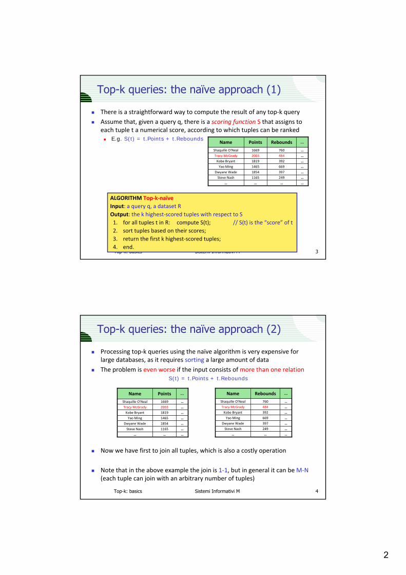
There is a straightforward way to compute the result of any top‐k queryAssume that, given a query q, there is a scoring function S that assigns to each tuple t a numerical score, according to which tuples can be ranked
E.g. S(t) = t.Points + t.Rebounds
ALGORITHM Top‐k‐naїveInput: a query q, a dataset ROutput: the k highest‐scored tuples with respect to S1. for all tuples t in R: compute S(t); // S(t) is the “score” of t2. sort tuples based on their scores;3. return the first k highest‐scored tuples;4. end.
…7601669Shaquille O'Neal
…2491165Steve Nash
…………
…3971854Dwyane Wade
…6691465Yao Ming
…3921819Kobe Bryant
…4842003Tracy McGrady
…ReboundsPointsName
Top-k: basics Sistemi Informativi M 4
Top-k queries: the naїve approach (2)
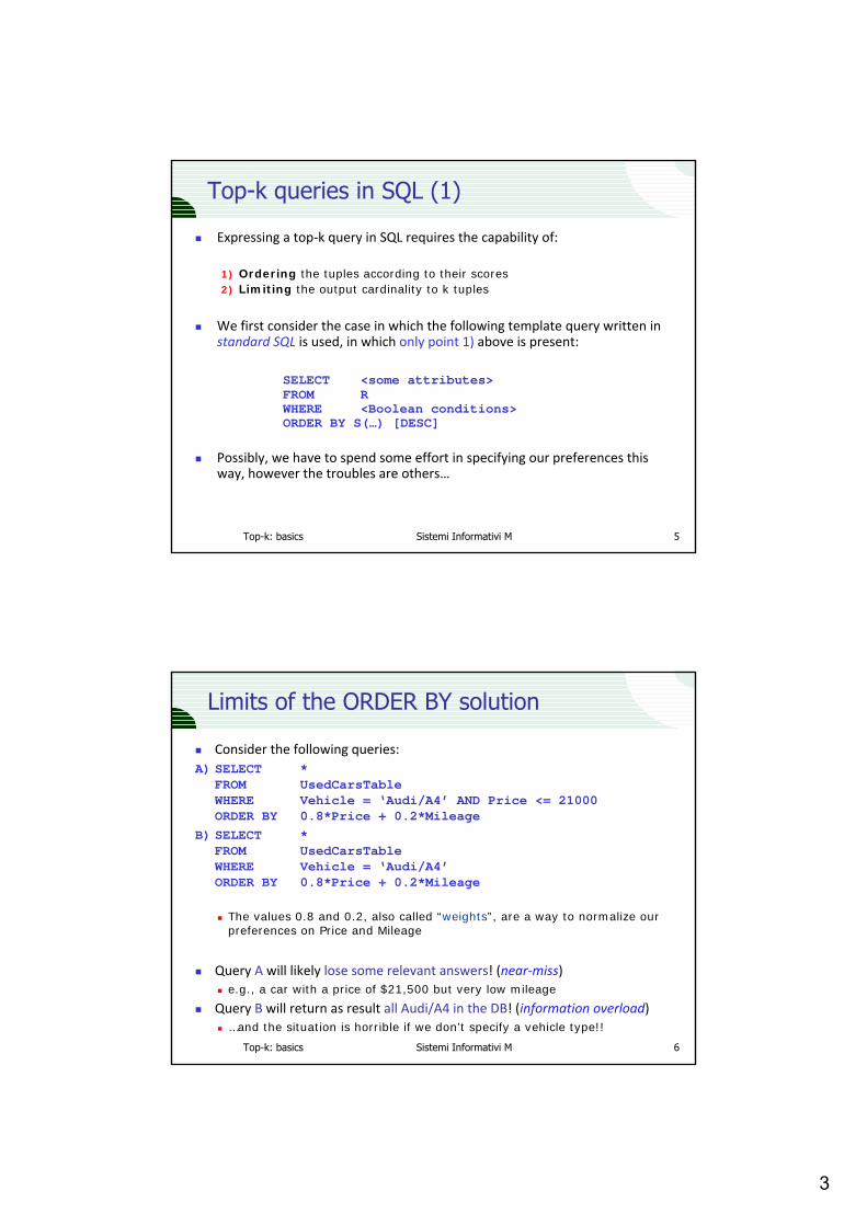
Processing top‐k queries using the naїve algorithm is very expensive for large databases, as it requires sorting a large amount of dataThe problem is even worse if the input consists of more than one relation
S(t) = t.Points + t.Rebounds
Now we have first to join all tuples, which is also a costly operation
Note that in the above example the join is 1‐1, but in general it can be M‐N(each tuple can join with an arbitrary number of tuples)
…760Shaquille O'Neal
…249Steve Nash
………
…397Dwyane Wade
…669Yao Ming
…392Kobe Bryant
…484Tracy McGrady
…ReboundsName
…1669Shaquille O'Neal
…1165Steve Nash
………
…1854Dwyane Wade
…1465Yao Ming
…1819Kobe Bryant
…2003Tracy McGrady
…PointsName
3
Top-k: basics Sistemi Informativi M 5
Top-k queries in SQL (1)
Expressing a top‐k query in SQL requires the capability of:
1) Ordering the tuples according to their scores2) Limiting the output cardinality to k tuples
We first consider the case in which the following template query written instandard SQL is used, in which only point 1) above is present:
SELECT <some attributes>FROM RWHERE <Boolean conditions>ORDER BY S(…) [DESC]
Possibly, we have to spend some effort in specifying our preferences thisway, however the troubles are others…
Top-k: basics Sistemi Informativi M 6
Limits of the ORDER BY solution
Consider the following queries:A) SELECT *
FROM UsedCarsTableWHERE Vehicle = ‘Audi/A4’ AND Price <= 21000ORDER BY 0.8*Price + 0.2*Mileage
B) SELECT *FROM UsedCarsTableWHERE Vehicle = ‘Audi/A4’ORDER BY 0.8*Price + 0.2*Mileage
The values 0.8 and 0.2, also called “weights”, are a way to normalize ourpreferences on Price and Mileage
Query A will likely lose some relevant answers! (near‐miss)e.g., a car with a price of $21,500 but very low mileage
Query B will return as result all Audi/A4 in the DB! (information overload)…and the situation is horrible if we don’t specify a vehicle type!!

4
Top-k: basics Sistemi Informativi M 7
ORDER BY solution & C/S architecture (1)
Before considering other solutions, let’s take a closer look at how the DBMS server sends the result of a query to the client applicationOn the client side we work “1 tuple at a time” by using, e.g., rs.next()
However this does not mean that a result set is shipped (transmitted) 1 tuple at a time from the server to the client!
Most (all?) DBMSs implement a feature known as row blocking, aiming at reducing the transmission overheadRow blocking:
1. The DBMS allocates some buffers (a “block”) on the server side2. It fills the buffers with tuples of the query result3. It ships the whole block of tuples to the client4. The client consumes (reads) the tuples in the block5. Repeat from 2 until no more tuples (rows) are in the result set
32
20
10
PriceOBJ
t16
t24
t07 40t21
38t14
……
46t06
block of tuples block
32
20
10
PriceOBJ
t16
t24
t07
Top-k: basics Sistemi Informativi M 8
Why row blocking is not enough? I.e.: why do we need “k”?
In DB2 the block size is established when the application connects to the DB (default size: 32 KB)If the buffers can hold, say, 1000 tuples but the application just looks at the first, say, 10, we waste resources:
We fetch from disk and process too many (1000) tuplesWe transmit too many data (1000 tuples) over the network
If we reduce the block size, then we might incur a large transmission overheadfor queries with large result sets
Bear in mind that we don’t have “just one query”: our application mightconsist of a mix of queries, each one with its own requirements
Also observe that the DBMS “knows nothing” about the client’s intention, i.e., it will optimize and evaluate the query so as to deliver the whole result set (more on this later)
ORDER BY solution & C/S architecture (2)
5
Top-k: basics Sistemi Informativi M 9
Top-k queries in SQL (2)
The first step to support top‐k queries is simple: extend SQL with a new clause that explicitly limits the cardinality of the result:
SELECT <some attributes>FROM <some relation(s)>WHERE <Boolean conditions>[GROUP BY <some grouping attributes>]ORDER BY S(…) [DESC]STOP AFTER k
where k is a positive integerThis is the syntax proposed in [CK97] (see references on the Web site), most DBMSs have proprietary (equivalent) extensions, e.g.:
FETCH FIRST k ROWS ONLY (DB2 UDB), LIMIT TO k ROWS(ORACLE), LIMIT k, …[CK97] also allows a numerical expression, uncorrelated with the rest of the query, in place of k
Top-k: basics Sistemi Informativi M 10
Semantics of top-k queries
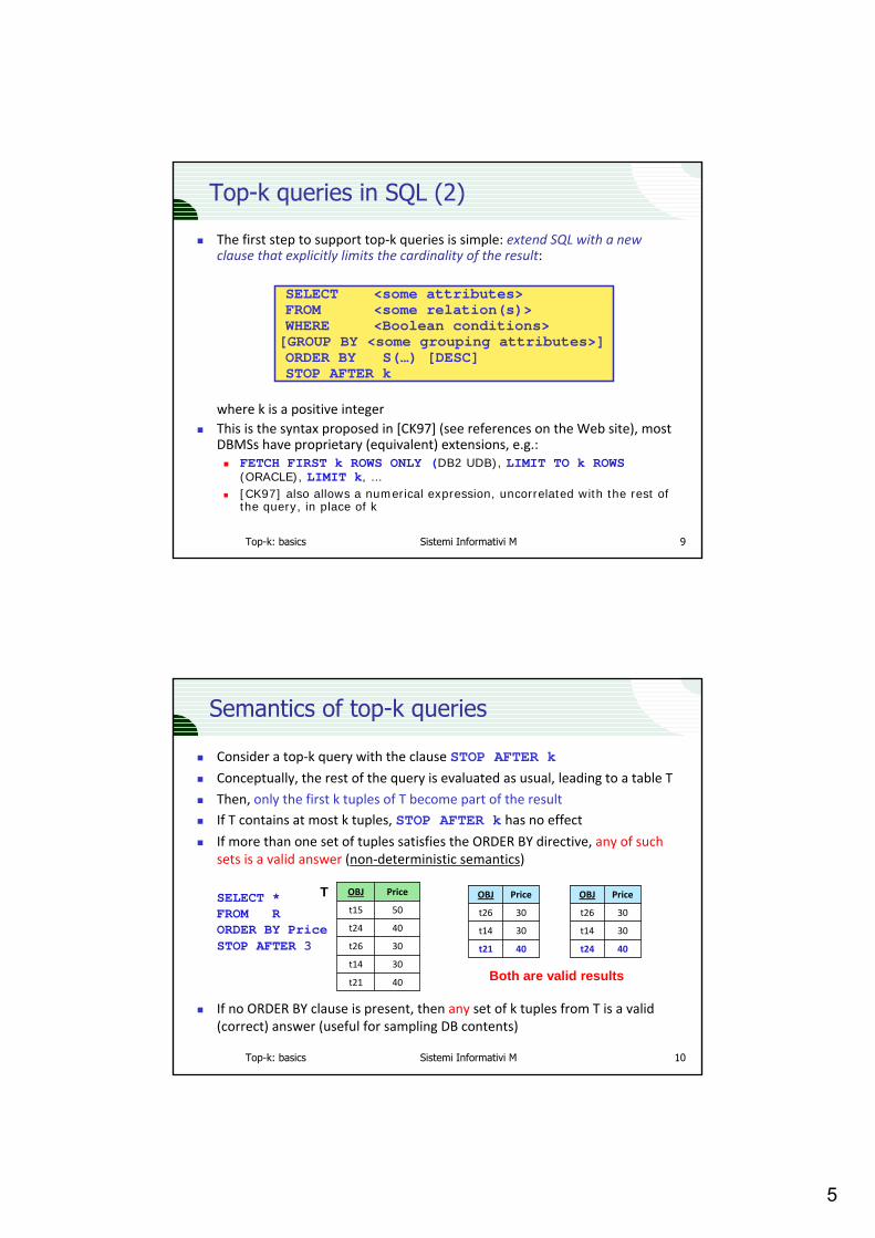
Consider a top‐k query with the clause STOP AFTER kConceptually, the rest of the query is evaluated as usual, leading to a table T
Then, only the first k tuples of T become part of the resultIf T contains at most k tuples, STOP AFTER k has no effect
If more than one set of tuples satisfies the ORDER BY directive, any of suchsets is a valid answer (non‐deterministic semantics)
SELECT *FROM RORDER BY PriceSTOP AFTER 3
If no ORDER BY clause is present, then any set of k tuples from T is a valid (correct) answer (useful for sampling DB contents)
40t21
30
30
40
50
PriceOBJ
t14
t26
t24
t15
T
Both are valid results
40t21
30
30
PriceOBJ
t14
t26
40t24
30
30
PriceOBJ
t14
t26
6
Top-k: basics Sistemi Informativi M 11
Top-k queries: examples (1)
The best NBA player (considering points and rebounds):SELECT *FROM NBAORDER BY Points + Rebounds DESCSTOP AFTER 1
The 2 cheapest chinese restaurantsSELECT *FROM RESTAURANTSWHERE Cuisine = `chinese’ORDER BY PriceSTOP AFTER 2
The top‐5% highest paid employees SELECT E.* -- a top-k query with a numerical expressionFROM EMP EORDER BY E.Salary DESCSTOP AFTER (SELECT COUNT(*)/20 FROM EMP)
Top-k: basics Sistemi Informativi M 12
Top-k queries: examples (2)
The top‐5 Audi/A4 (based on price and mileage)SELECT *FROM USEDCARSWHERE Vehicle = ‘Audi/A4’ORDER BY 0.8*Price + 0.2*MileageSTOP AFTER 5
The 2 hotels closest to the Bologna airportSELECT H.* -- a top-k distance join queryFROM HOTELS H, AIRPORTS AWHERE A.Code = ‘BLQ’ORDER BY distance(H.Location,A.Location)STOP AFTER 2
Location is a “point” UDT (User-defined Data Type) distance is a UDF (User-Defined Function)
7
Top-k: basics Sistemi Informativi M 13
UDT’s and UDF’s
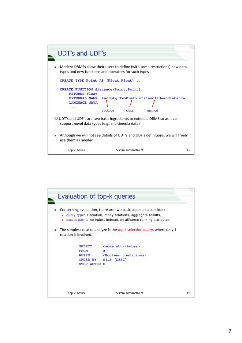
Modern DBMSs allow their users to define (with some restrictions) new data types and new functions and operators for such types
CREATE TYPE Point AS (Float,Float) ...
CREATE FUNCTION distance(Point,Point) RETURNS Float EXTERNAL NAME ‘twodpkg.TwoDimPoints!euclideandistance’LANGUAGE JAVA...
☺ UDT’s and UDF’s are two basic ingredients to extend a DBMS so as it can support novel data types (e.g., multimedia data)
Although we will not see details of UDT’s and UDF’s definitions, we will freelyuse them as needed
package class method
Top-k: basics Sistemi Informativi M 14
Evaluation of top-k queries
Concerning evaluation, there are two basic aspects to consider:query type: 1 relation, many relations, aggregate results, …access paths: no index, indexes on all/some ranking attributes
The simplest case to analyze is the top‐k selection query, where only 1 relation is involved:
SELECT <some attributes>FROM RWHERE <Boolean conditions>ORDER BY S(…) [DESC]STOP AFTER k
8
Top-k: basics Sistemi Informativi M 15
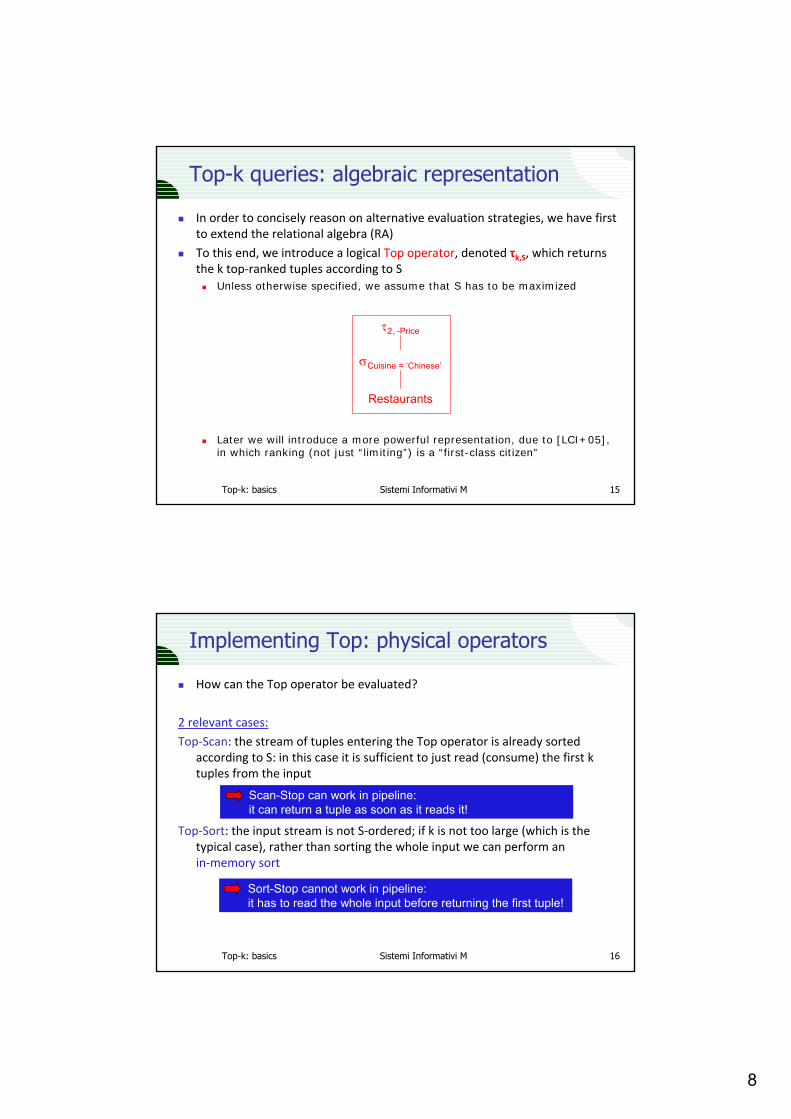
Top-k queries: algebraic representation
In order to concisely reason on alternative evaluation strategies, we have first to extend the relational algebra (RA)To this end, we introduce a logical Top operator, denoted τk,S, which returns the k top‐ranked tuples according to S
Unless otherwise specified, we assume that S has to be maximized
Later we will introduce a more powerful representation, due to [LCI+05], in which ranking (not just “limiting”) is a “first-class citizen”
Restaurants
σCuisine = ‘Chinese’
τ2, -Price
Top-k: basics Sistemi Informativi M 16
Implementing Top: physical operators
How can the Top operator be evaluated?
2 relevant cases:Top‐Scan: the stream of tuples entering the Top operator is already sorted
according to S: in this case it is sufficient to just read (consume) the first k tuples from the input
Top‐Sort: the input stream is not S‐ordered; if k is not too large (which is the typical case), rather than sorting the whole input we can perform anin‐memory sort
Scan-Stop can work in pipeline: it can return a tuple as soon as it reads it!
Sort-Stop cannot work in pipeline: it has to read the whole input before returning the first tuple!
9
Top-k: basics Sistemi Informativi M 17
Physical operators: the iterator interface
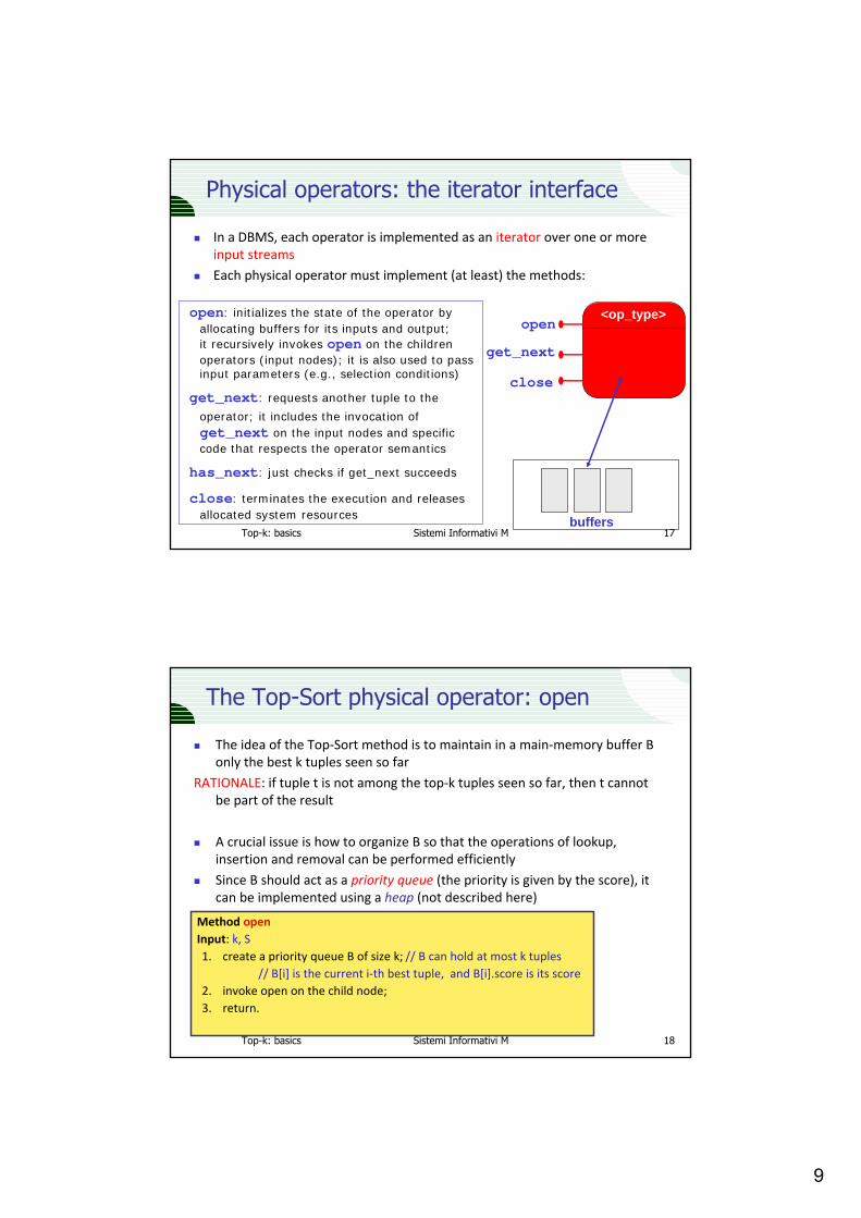
In a DBMS, each operator is implemented as an iterator over one or more input streamsEach physical operator must implement (at least) the methods:
open: initializes the state of the operator by allocating buffers for its inputs and output; it recursively invokes open on the children operators (input nodes); it is also used to pass input parameters (e.g., selection conditions)
get_next: requests another tuple to the
operator; it includes the invocation ofget_next on the input nodes and specific code that respects the operator semantics
has_next: just checks if get_next succeeds
close: terminates the execution and releases allocated system resources
open
get_next
close
<op_type>
buffers
Top-k: basics Sistemi Informativi M 18
The Top-Sort physical operator: open
The idea of the Top‐Sort method is to maintain in a main‐memory buffer B only the best k tuples seen so far
RATIONALE: if tuple t is not among the top‐k tuples seen so far, then t cannot be part of the result
A crucial issue is how to organize B so that the operations of lookup, insertion and removal can be performed efficiently
Since B should act as a priority queue (the priority is given by the score), it can be implemented using a heap (not described here)
Method openInput: k, S1. create a priority queue B of size k; // B can hold at most k tuples
// B[i] is the current i‐th best tuple, and B[i].score is its score2. invoke open on the child node;3. return.
10
Top-k: basics Sistemi Informativi M 19
The Top-Sort physical operator: get_next
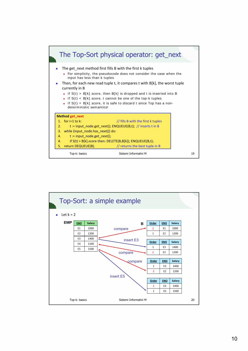
The get_next method first fills B with the first k tuplesFor simplicity, the pseudocode does not consider the case when the input has less than k tuples
Then, for each new read tuple t, it compares t with B[k], the worst tuple currently in B
If S(t) > B[k].score, then B[k] is dropped and t is inserted into BIf S(t) < B[k].score, t cannot be one of the top-k tuplesIf S(t) = B[k].score, it is safe to discard t since Top has a non-deterministic semantics!
Method get_next1. for i=1 to k: // fills B with the first k tuples2. t := input_node.get_next(); ENQUEUE(B,t); // inserts t in B3. while (input_node.has_next()) do:4. t := input_node.get_next();4. if S(t) > B[k].score then: DELETE(B,B[k]); ENQUEUE(B,t);5. return DEQUEUE(B). // returns the best tuple in B
Top-k: basics Sistemi Informativi M 20
Top-Sort: a simple example
Let k = 2
1500E5
1100
1400
1200
1000
SalaryENO
E4
E3
E2
E1
1
2
Order
1200
1000
SalaryENO
E2
E1
EMP B
2
1
Order
1200
1400
SalaryENO
E2
E3
compare
insert E3
2
1
Order
1200
1400
SalaryENO
E2
E3
compare
compare
1
2
Order
1500
1400
SalaryENO
E5
E3
insert E5

11
Top-k: basics Sistemi Informativi M 21
Experimental results from [CK97] (1)
SELECT E.* FROM EMP EORDER BY E.Salary DESCSTOP AFTER N;
In-memory sort
No Index available
The naïve method sorts ALL the tuples!
TRADITIONAL = row blocking(about 500 tuples)TRAD(NRB) = no row blocking
Top-k: basics Sistemi Informativi M 22
Results from [CK97] (2)
SELECT E.* FROM EMP EORDER BY E.Salary DESCSTOP AFTER N;
Both TRADITIONAL and TRAD(NRB) still scan and sort the whole table
Unclustered Index on Emp.Salary
If the DBMS ignores that we just need k tuples, it will not use the index: it will scan the EMP table and then sort ALL the N tuples!
12
Top-k: basics Sistemi Informativi M 23
Results from [CK97] (3)
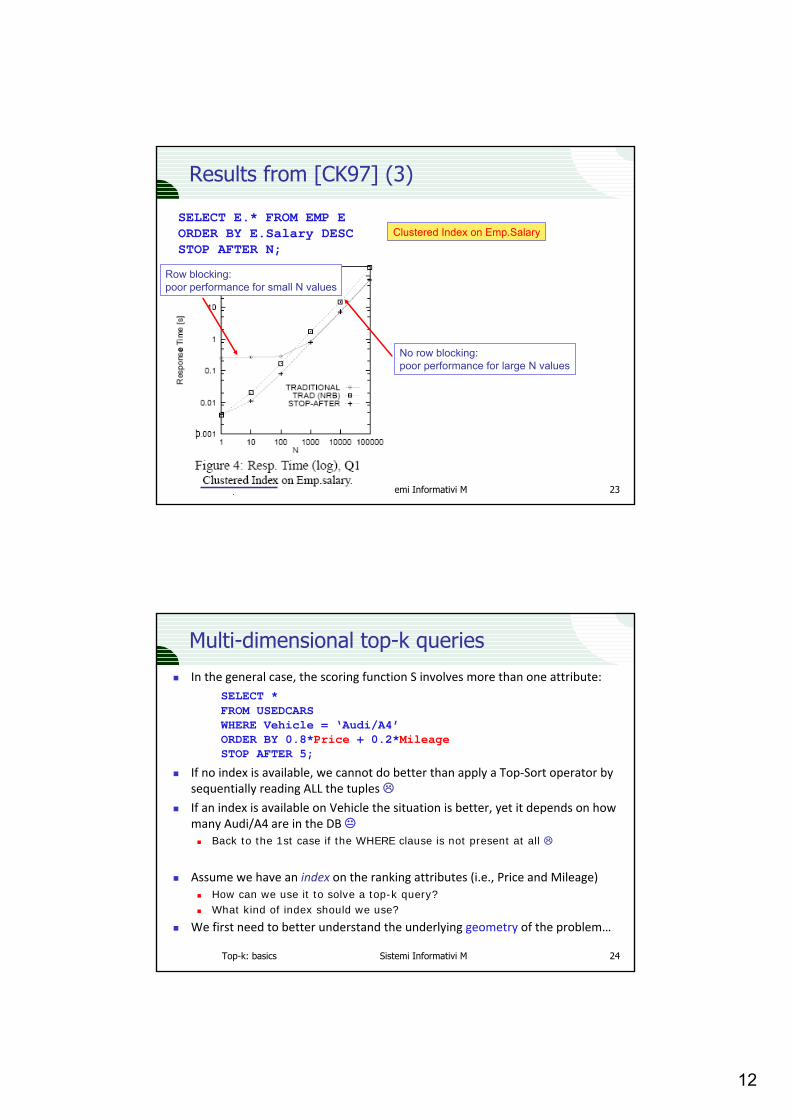
SELECT E.* FROM EMP EORDER BY E.Salary DESCSTOP AFTER N;
Row blocking: poor performance for small N values
No row blocking: poor performance for large N values
Clustered Index on Emp.Salary
Top-k: basics Sistemi Informativi M 24
Multi-dimensional top-k queries
In the general case, the scoring function S involves more than one attribute:SELECT *FROM USEDCARSWHERE Vehicle = ‘Audi/A4’ORDER BY 0.8*Price + 0.2*MileageSTOP AFTER 5;
If no index is available, we cannot do better than apply a Top‐Sort operator bysequentially reading ALL the tuples
If an index is available on Vehicle the situation is better, yet it depends on howmany Audi/A4 are in the DB
Back to the 1st case if the WHERE clause is not present at all
Assume we have an index on the ranking attributes (i.e., Price and Mileage)How can we use it to solve a top-k query? What kind of index should we use?
We first need to better understand the underlying geometry of the problem…

13
Top-k: basics Sistemi Informativi M 25
The “attribute space”: a geometric view
Consider the 2‐dimensional (2‐dim) attribute space (Price,Mileage)
0
10
20
30
40
50
60
0 10 20 30 40 50Price
Mile
age
C1C2
C3C4
C5
C6
C7
C8C9
C10
C11
Each tuple is represented by a 2-dim point (p,m):
p is the Price valuem is the Mileage value
Intuitively, minimizing0.8*Price + 0.2*Mileage
is equivalent to look for points“close” to (0,0)(0,0) is our (ideal) “target value”(i.e., a free car with 0 km’s!)
Top-k: basics Sistemi Informativi M 26
The role of weights (preferences)Our preferences (e.g., 0.8 and 0.2) are essential to determine the result
With preferences (0.8,0.2) the best car is C6, then C5, etc.In general, preferences are a way to determine, given points (p1,m1) and (p2,m2), which of them is “closer” to the target point (0,0)
0
10
20
30
40
50
60
0 10 20 30 40 50Price
Mile
age
C1C2
C3C4
C5
C6
C7
C8C9
C10
C11
Consider the line l(v) of equation0.8*Price + 0.2*Mileage = v
where v is a constantThis can also be written asMileage = -4*Price + 5*v
from which we see that all the lines l(v) have a slope = -4By definition, all the points of l(v) are “equally good” to us
v=20 v=34v=16

14
Top-k: basics Sistemi Informativi M 27
Changing the weightsClearly, changing the weight values will likely lead to a different result
On the other hand, if weights do not change too much, the results of two top‐k queries will likely have a high degree of overlap
0
10
20
30
40
50
60
0 10 20 30 40 50Price
Mile
age
C1C2
C3C4
C5
C6
C7
C8C9
C10
C11
With0.8*Price + 0.2*Mileage
the best car is C6With0.5*Price + 0.5*Mileage
the best cars are C5 and C11
v=20
v=16 0.8*Price + 0.2*Mileage
0.5*Price + 0.5*Mileage
Top-k: basics Sistemi Informativi M 28
Changing the targetThe target of a query is not necessarily (0,0), rather it can be any pointq=(q1,q2) (qi = query value for the i‐th attribute) Example: assume you are looking for a house with a 1000 m2 garden and 3 bedrooms; then (1000,3) is the target for your query
1
2
3
4
5
0 500 1000 1500 2000Garden
Bed
room
s
In general, in order to determinethe “goodness” of a tuple t, we compute its “distance” fromthe target point q:The lower the distance from q,
the better t is
Note that distance values can always be converted into goodness “scores”, so that a higher score means a better matchJust change the sign and possibly add a constant,…
q

15
Top-k: basics Sistemi Informativi M 29
Top-k tuples = k-nearest neighbors
In order to provide a homogeneous management of the problem when using an index, it is useful to consider distances rather than scores
since most indexes are “distance-based”
Therefore, the model is now:A D-dimensional (D≥1) attribute space A = (A1,A2,…,AD) of ranking attributesA relation R(A1,A2,…,AD,B1,B2,…), where B1,B2,… are other attributesA target (query) point q = (q1,q2,…,qD), q ∈ AA function d: A x A → ℜ, that measures the distance between points of A (e.g., d(t,q) is the distance between t and q)
Under this model, a top‐k query is transformed into a so‐called
k-Nearest Neighbors (k-NN) QueryGiven a point q, a relation R, an integer k ≥ 1, and a distance function dDetermine the k tuples in R that are closest to q according to d
Top-k: basics Sistemi Informativi M 30
Some common distance functionsThe most commonly used distance functions are Lp‐norms:
Relevant cases are:
1/pD
1i
piip qtq)(t,L ⎟⎠
⎞⎜⎝
⎛−= ∑
=
{ } distance(max)Chebyshev
distanceblock)(cityManhattan
distanceEuclidean
iii
D
1iii1
D
1i
2ii2
qtmaxq)(t,L
qtq)(t,L
qtq)(t,L
−=
−−=
−=
∞
=
=
∑
∑
Iso-distance (hyper-)surfaces
q
q
q

16
Top-k: basics Sistemi Informativi M 31
Shaping the attribute space
Changing the distance function leads to a different shaping of the attributespace (each colored “stripe” in the figures corresponds to points withdistance values between v and v+1, v integer)
L1; q=(7,12)
1 3 5 7 9 11 13 15 17 19135791113151719
A1
A2
1 3 5 7 9 11 13 15 17 191357
91113151719
A1
A2
L2; q=(7,12)
Note that, for 2 tuples t1 and t2, it is possible to haveL1(t1,q) < L1(t2,q) and L2(t2,q) < L2(t1,q)
E.g.: t1=(13,12)t2=(12,10)
Top-k: basics Sistemi Informativi M 32
Distance functions with weightsThe use of weights just leads to “stretch” some of the coordinates:
{ }iiii
D
1iiii1
D
1i
2iii2
qtwmaxW)q;(t,L
qtwW)q;(t,L
qtwW)q;(t,L
−=
−=
−=
∞
=
=
∑
∑ (hyper-)ellipsoids
(hyper-)romboids
(hyper-)rectangles
Thus, the scoring function0.8*Price + 0.2*Mileage
is just a particular case of weighted L1distance
17
Top-k: basics Sistemi Informativi M 33
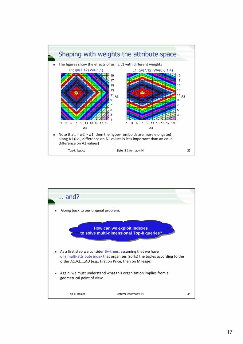
Shaping with weights the attribute spaceThe figures show the effects of using L1 with different weights
Note that, if w2 > w1, then the hyper‐romboids are more elongatedalong A1 (i.e., difference on A1 values is less important than an equaldifference on A2 values)
1 3 5 7 9 11 13 15 17 19135791113151719
A1
A2
1 3 5 7 9 11 13 15 17 191357
91113151719
A1
A2
L1; q=(7,12) W=(1,1) L1; q=(7,12) W=(0.6,1.4)
Top-k: basics Sistemi Informativi M 34
… and?
Going back to our original problem:
As a first step we consider B+‐trees, assuming that we haveone multi‐attribute index that organizes (sorts) the tuples according to the order A1,A2,…,AD (e.g., first on Price, then on Mileage)
Again, we must understand what this organization implies from a geometrical point of view…
How can we exploit indexesto solve multi-dimensional Top-k queries?
18
Top-k: basics Sistemi Informativi M 35
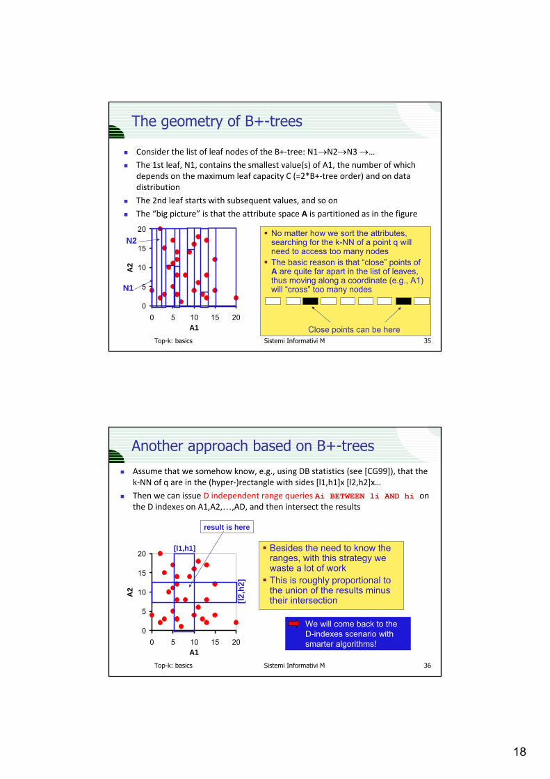
The geometry of B+-trees
Consider the list of leaf nodes of the B+‐tree: N1→N2→N3 →…The 1st leaf, N1, contains the smallest value(s) of A1, the number of whichdepends on the maximum leaf capacity C (=2*B+‐tree order) and on data distribution
The 2nd leaf starts with subsequent values, and so onThe “big picture” is that the attribute space A is partitioned as in the figure
0
5
10
15
20
0 5 10 15 20A1
A2
N1
N2No matter how we sort the attributes, searching for the k-NN of a point q willneed to access too many nodesThe basic reason is that “close” points of A are quite far apart in the list of leaves, thus moving along a coordinate (e.g., A1) will “cross” too many nodes
Close points can be here
Top-k: basics Sistemi Informativi M 36
Another approach based on B+-trees
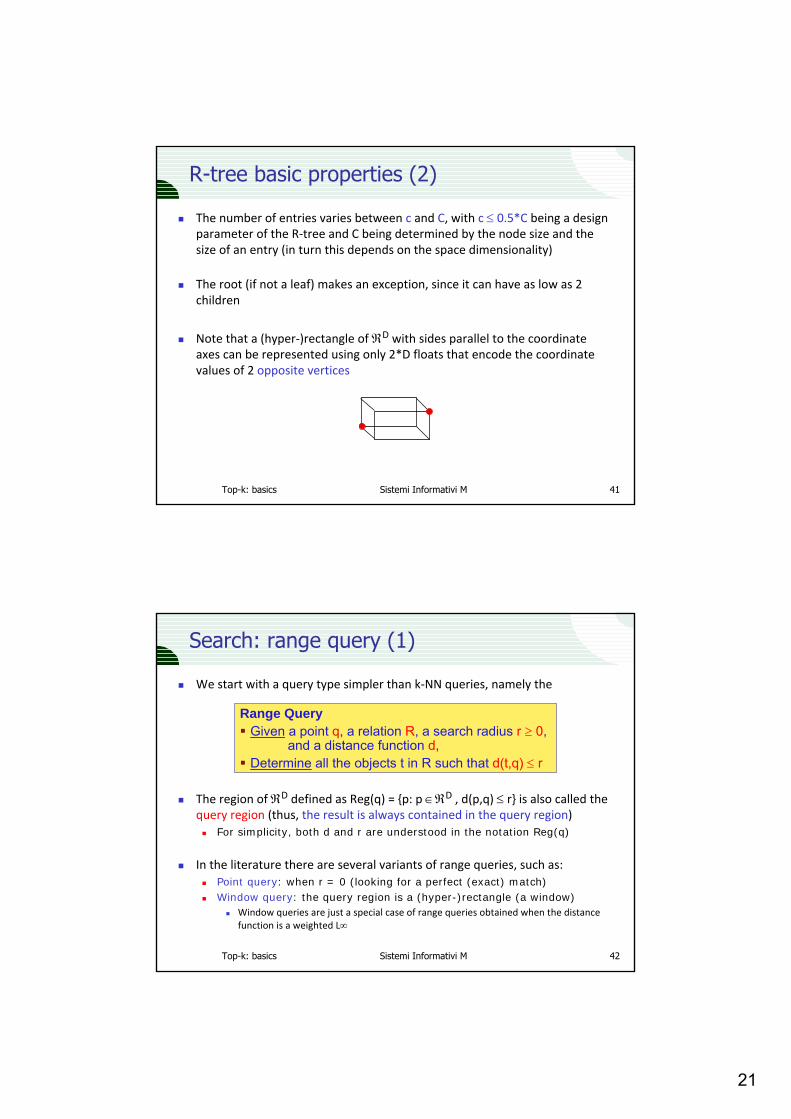
Assume that we somehow know, e.g., using DB statistics (see [CG99]), that the k‐NN of q are in the (hyper‐)rectangle with sides [l1,h1]x [l2,h2]x…
Then we can issue D independent range queries Ai BETWEEN li AND hi on the D indexes on A1,A2,…,AD, and then intersect the results
0
5
10
15
20
0 5 10 15 20A1
A2
[l2,h
2]
[l1,h1] Besides the need to know the ranges, with this strategy wewaste a lot of workThis is roughly proportional tothe union of the results minustheir intersection
result is here
We will come back to the D-indexes scenario withsmarter algorithms!

19
Top-k: basics Sistemi Informativi M 37
Multi-dimensional (spatial) indexes
The multi‐attribute B+‐tree maps points of A ⊆ℜD into points of ℜThis “linearization”necessarily favors, depending on how attributes are ordered in the B+‐tree, one attribute with respect to others
A B+-tree on (X,Y) favors queries on X, it cannot be used for queriesthat do not specify a restriction on X
Therefore, what we need is a way to organize points so as to preserve, asmuch as possible, their “spatial proximity”
The issue of “spatial indexing” has been under investigation since the 70’s, because of the requirements of applications dealing with “spatial data”(e.g., cartography, geographic information systems, VLSI, CAD)
More recently (starting from the 90’s), there has been a resurrection of interest in the problem due to the new challenges posed by several otherapplication scenarios, such as multimedia and data miningWe will now just consider one (indeed very relevant!) spatial index…
Top-k: basics Sistemi Informativi M 38
The R-tree (Guttman, 1984)
The R‐tree [Gut84] is (somewhat) an extension of the B+‐tree to multi‐dimensional spaces, in that:The B+‐tree organizes objects into
a set of (non-overlapping) 1-D intervals, and then applies recursively this basic principle up to the root,
the R‐tree does the same but now using a set of (possibly overlapping) m-D intervals, i.e., (hyper-)rectangles,and then applies recursively this basic principle up to the root
The R‐tree is also available in some commercial DBMS’s, such as OracleIn the following we just present the aspects relevant to query processing

20
Top-k: basics Sistemi Informativi M 39
GDE
HF
P ON
L
I
JK
M
A
C
B
A B C
Recursive bottom-up aggregation of objects based on MBR’sRegions can overlap
…………………………...D P
N O PI J K L MD E F G HA B C
R-tree: The intuition
This is a 2-D range queryusing L2, other queries and distance functionscan be supported as well
Top-k: basics Sistemi Informativi M 40
R-tree basic properties (1)
The R‐tree is a dynamic, height‐balanced, and paged treeEach node stores a variable number of entries
Leaf node:An entry E has the form E=(tuple-key,TID), where tuple-key is the “spatial key” (position) of the tuple whose address is TID (remind: TID is a pointer)
Internal node:An entry E has the form E=(MBR,PID), where MBR is the “Minimum Bounding Rectangle” (with sides parallel to the coordinate axes) of all the points reachable from (“under”) the child node whose address is PID (PID = page identifier) A B C
DI J K L MD E F G H
A BWe can uniform things by sayingthat each entry has the format
E=(key,ptr)If N is the node pointed by E.ptr, then E.key is the “spatial key” of N E=(tuple-key,TID)
E=(MBR,PID)
21
Top-k: basics Sistemi Informativi M 41
R-tree basic properties (2)
The number of entries varies between c and C, with c ≤ 0.5*C being a design parameter of the R‐tree and C being determined by the node size and the size of an entry (in turn this depends on the space dimensionality)
The root (if not a leaf) makes an exception, since it can have as low as 2 children
Note that a (hyper‐)rectangle of ℜD with sides parallel to the coordinate axes can be represented using only 2*D floats that encode the coordinate values of 2 opposite vertices
Top-k: basics Sistemi Informativi M 42
Search: range query (1)
We start with a query type simpler than k‐NN queries, namely the
The region of ℜD defined as Reg(q) = {p: p ∈ℜD , d(p,q) ≤ r} is also called the query region (thus, the result is always contained in the query region)
For simplicity, both d and r are understood in the notation Reg(q)
In the literature there are several variants of range queries, such as:Point query: when r = 0 (looking for a perfect (exact) match)Window query: the query region is a (hyper-)rectangle (a window)
Window queries are just a special case of range queries obtained when the distance function is a weighted L∞
Range QueryGiven a point q, a relation R, a search radius r ≥ 0,
and a distance function d, Determine all the objects t in R such that d(t,q) ≤ r

22
Top-k: basics Sistemi Informativi M 43
Search: range query (2)
The algorithm for processing a range query is extremely simple:We start from the root and, for each entry E in the root node, we check ifE.key intersects Reg(q):
Reg(q) ∩ E.key ≠ ∅: we access the child node N referenced by E.ptrReg(q) ∩ E.key = ∅: we can discard node N from the search
When we arrive at a leaf node we just check for each entry E ifE.key ∈ Reg(q), that is, if d(E.key,q) ≤ r.
If this is the case we can add E to the result of the index search
The recursion starts from the root of the R‐treeThe notation N = *(E.ptr) means “N is the node pointed by E.ptr”Sometimes we also write ptr(N) in place of E.ptr
RangeQuery(q,r,N){ if N is a leaf then: for each E in N:
if d(E.key,q) ≤ r then add E to the resultelse: for each E in N:
if Req(q) ∩ E.key ≠ ∅ then RangeQuery(q,r,*(E.ptr) }
Top-k: basics Sistemi Informativi M 44
GDE
HF
P ON
L
I
JK
M
A
C
BThe navigation follows a depth-first patternThis ensures that, at eachtime step, the maximumnumber of nodes in memoryis h=height of the R-treeSuch nodes are managedusing a stack
…
Range queries in action
A B C
I J K L MD E F G H…
…

23
Top-k: basics Sistemi Informativi M 45
Search: k-NN query (1)With the aim to better understand the logic of k‐NN search, let us define for a node N = *(E.ptr) of the R‐tree its region as
Reg(*(E.ptr)) = Reg(N) = {p: p ∈ℜD , p ∈ E.key=E.MBR}
Thus, we access node N if and only if (iff) Req(q) ∩ Reg(N) ≠ ∅Let us now define dMIN(q,Reg(N)) = infp{d(q,p) | p ∈ Reg(N)},that is, the minimum possible distance between q and a point in Reg(N)
The “MinDist” dMIN(q,Reg(N)) is a lower bound on the distances from q to any indexed point reachable from N
dMIN(q,Reg(N1))
dMIN(q,Reg(N2))dMIN(q,Reg(N3))
N1
N2
N3We can make the following basic observation:
Reg(q) ∩ Reg(N) ≠ ∅⇔
dMIN(q,Reg(N)) ≤ r
r
Top-k: basics Sistemi Informativi M 46
Search: k-NN query (2)We now present an algorithm, called kNNOptimal [BBK+97], for solving k‐NNqueries with an R‐tree that is I/O‐optimal
The algorithm also applies to other index structures (e.g., the M-tree) that we will see in this course
We start with the basic case k=1
For a given query point q, let tNN(q) be the 1st nearest neighbor (1‐NN = NN) of q in R, and denote with rNN = d(q, tNN(q)) its distance from q
Clearly, rNN is only known when the algorithm terminates
Theorem:Any correct algorithm for 1‐NN queries must visit at least all the nodes N whose MinDist is strictly less than rNN, i.e., dMIN(q,Reg(N)) < rNN
Proof: Assume that an algorithm A stops by reporting as NN of q a point t,and that A does not read a node N such that (s.t.) dMIN(q,Reg(N)) < d(q,t); then Reg(N) might contain a point t’ s.t. d(q,t’) < d(q,t), thus contradicting the hypothesis that t is the NN of q
24
Top-k: basics Sistemi Informativi M 47
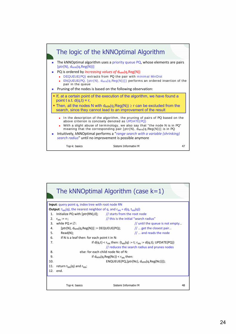
The logic of the kNNOptimal AlgorithmThe kNNOptimal algorithm uses a priority queue PQ, whose elements are pairs[ptr(N), dMIN(q,Reg(N))]PQ is ordered by increasing values of dMIN(q,Reg(N))
DEQUEUE(PQ) extracts from PQ the pair with minimal MinDistENQUEUE(PQ, [ptr(N), dMIN(q,Reg(N))]) performs an ordered insertion of the pair in the queue
Pruning of the nodes is based on the following observation:
In the description of the algorithm, the pruning of pairs of PQ based on the above criterion is concisely denoted as UPDATE(PQ)With a slight abuse of terminology, we also say that “the node N is in PQ”meaning that the corresponding pair [ptr(N), dMIN(q,Reg(N))] is in PQ
Intuitively, kNNOptimal performs a “range search with a variable (shrinking) search radius” until no improvement is possible anymore
If, at a certain point of the execution of the algorithm, we have found a point t s.t. d(q,t) = r, Then, all the nodes N with dMIN(q,Reg(N)) ≥ r can be excluded from the search, since they cannot lead to an improvement of the result
Top-k: basics Sistemi Informativi M 48
The kNNOptimal Algorithm (case k=1)
Input: query point q, index tree with root node RNOutput: tNN(q), the nearest neighbor of q, and rNN = d(q, tNN(q))1. Initialize PQ with [ptr(RN),0]; // starts from the root node2. rNN := ∞; // this is the initial “search radius”3. while PQ ≠∅: // until the queue is not empty…4. [ptr(N), dMIN(q,Reg(N))] := DEQUEUE(PQ); // … get the closest pair…5. Read(N); // … and reads the node6. if N is a leaf then: for each point t in N:7. if d(q,t) < rNN then: {tNN(q) := t; rNN := d(q,t); UPDATE(PQ)}
// reduces the search radius and prunes nodes8. else: for each child node Nc of N:9. if dMIN(q,Reg(Nc)) < rNN then:10. ENQUEUE(PQ,[ptr(Nc), dMIN(q,Reg(Nc))]);11. return tNN(q) and rNN;12. end.

25
Top-k: basics Sistemi Informativi M 49
kNNOptimal in action
q
RN
N5
N7
N2
N4Nodes are numberedfollowing the order in which they are accessedObjects are numbered asthey are found toimprove (reduce) the search radiusThe accessed leaf nodesare shown in red
N3
t1
N1
N6t2
Top-k: basics Sistemi Informativi M 50
kNNOptimal: The best used car
C1
C2
C3
C4
C5
C6
C7
C8
C9
C10
C11
Read(N5)
(N2,19)(N1,16.4)Read(RN)(N4,22.9)
Return(C6,19)
Read(N2)Read(N3)Read(N1)
Action
(N2,19)
PQ
(N5,19)(N2,19)(N3,16.4)
N1
N2
N3
N4
N5 N6
d = 0.7*Price + 0.3*Mileage
0
10
20
30
40
50
60
0 10 20 30 40 50Price
Mile
age
19N526N6
22.916.41916.4
dMINNode
N4N3N2N1
…241920
dtuple
…C11C6C5

26
Top-k: basics Sistemi Informativi M 51
Correctness and optimality of kNNOptimalThe kNNOptimal algorithm is clearly correctTo show that it is also I/O‐optimal, that is, it reads the minimum number of nodes, it is sufficient to prove the following
Theorem:The kNNOptimal algorithm for 1‐NN queries never reads a node N whose MinDist is strictly larger than rNN, i.e., dMIN(q,Reg(N)) > rNN
Proof:Node N is read only if, at some execution step, it becomes the 1st element in PQLet N1 be the node containing tNN(q) , N2 its parent node, N3 the parent node of N2, and so on, up to Nh = RN (h = height of the tree) Now observe that, by definition of MinDist, it is:
rNN ≥ dMIN(q,Reg(N1)) ≥ dMIN(q,Reg(N2)) ≥ … ≥ dMIN(q,Reg(Nh))At each time step before we find tNN(q), one (and only one) of the nodesN1,N2,…,Nh is in the priority queueIt follows that N can never become the 1st element of PQ
Top-k: basics Sistemi Informativi M 52
What if dMIN(q,Reg(N)) = rNN? Q: The optimality theorem says nothing about regions whose MinDist equals the
NN distance. Why?
A: Because it cannot!
Note that all such regions tie, thus their relative ordering in PQ is undetermined. The possible cases are:
1. The NN is in a node whose region has MinDist < rNN. In this case no node with dMIN(q,Reg(N)) = rNN will be read
2. The NN is in a node whose region has exactly MinDist = rNN. Now everything depends on how ties are managed in PQ. In the worst case, all nodes with dMIN(q,Reg(N)) = rNN will be read
27
Top-k: basics Sistemi Informativi M 53
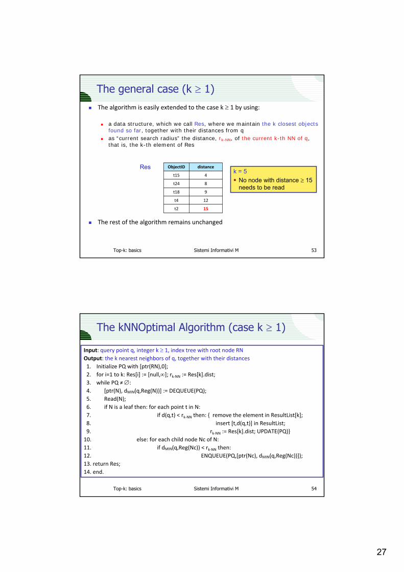
The general case (k ≥ 1)The algorithm is easily extended to the case k ≥ 1 by using:
a data structure, which we call Res, where we maintain the k closest objectsfound so far, together with their distances from qas “current search radius” the distance, rk-NN, of the current k-th NN of q, that is, the k-th element of Res
The rest of the algorithm remains unchanged
15t2
12
9
8
4
distanceObjectID
t4
t18
t24
t15
Resk = 5
No node with distance ≥ 15 needs to be read
Top-k: basics Sistemi Informativi M 54
The kNNOptimal Algorithm (case k ≥ 1)
Input: query point q, integer k ≥ 1, index tree with root node RNOutput: the k nearest neighbors of q, together with their distances1. Initialize PQ with [ptr(RN),0]; 2. for i=1 to k: Res[i] := [null,∞]; rk‐NN := Res[k].dist;3. while PQ ≠∅:4. [ptr(N), dMIN(q,Reg(N))] := DEQUEUE(PQ);5. Read(N); 6. if N is a leaf then: for each point t in N:7. if d(q,t) < rk‐NN then: { remove the element in ResultList[k];8. insert [t,d(q,t)] in ResultList;9. rk‐NN := Res[k].dist; UPDATE(PQ)}10. else: for each child node Nc of N:11. if dMIN(q,Reg(Nc)) < rk‐NN then:12. ENQUEUE(PQ,[ptr(Nc), dMIN(q,Reg(Nc))]);13. return Res;14. end.
28
Top-k: basics Sistemi Informativi M 55
Distance browsingNow we know how to solve top‐k selection queries using a multi‐dimensionalindex; but, what if our query isSELECT *FROM USEDCARSWHERE Vehicle = ‘Audi/A4’ORDER BY 0.8*Price + 0.2*MileageSTOP AFTER 5;
and we have an R‐tree on (Price,Mileage) built over ALL the cars?The k = 5 best matches returned by the index will not necessarily be Audi/A4
In this case we can use a variant of kNNOptimal, which supportsthe so‐called “distance browsing” [HS99] or “incremental NN queries”
For the case k = 1 the overall logic for using the index is:get from the index the 1st NNif it satisfies the query conditions (e.g., AUDI/A4) then stop,
otherwise get the next (2nd) NN and do the sameuntil 1 object is found that satisfies the query conditions
Top-k: basics Sistemi Informativi M 56
The get_next_NN algorithmIn the queue PQ now we keep both tuples and nodes
If an entry of PQ is tuple t then its distance d(q,t) is written dMIN(q,Reg(t))
Note that no pruning is possible (since we don’t know how many objects have tobe returned before stopping)
Before making the first call to the algorithm we initialize PQ with [ptr(RN),0]When a tuple t becomes the 1st element of the queue the algorithm returns
Input: query point q, index tree with root node RNOutput: the next nearest neighbor of q, together with its distance
1. while PQ ≠ ∅:2. [ptr(Elem), dMIN(q,Reg(Elem))] := DEQUEUE(PQ); 3. if Elem is a tuple t then: return t and its distance // no tuple can be better than t4. else: if N is a leaf then: for each point t in N: ENQUEUE(PQ,[t,d(q,t)])5. else: for each child node Nc of N: 6. ENQUEUE(PQ,[ptr(Nc), dMIN(q,Reg(Nc))]);7. end.
29
Top-k: basics Sistemi Informativi M 57
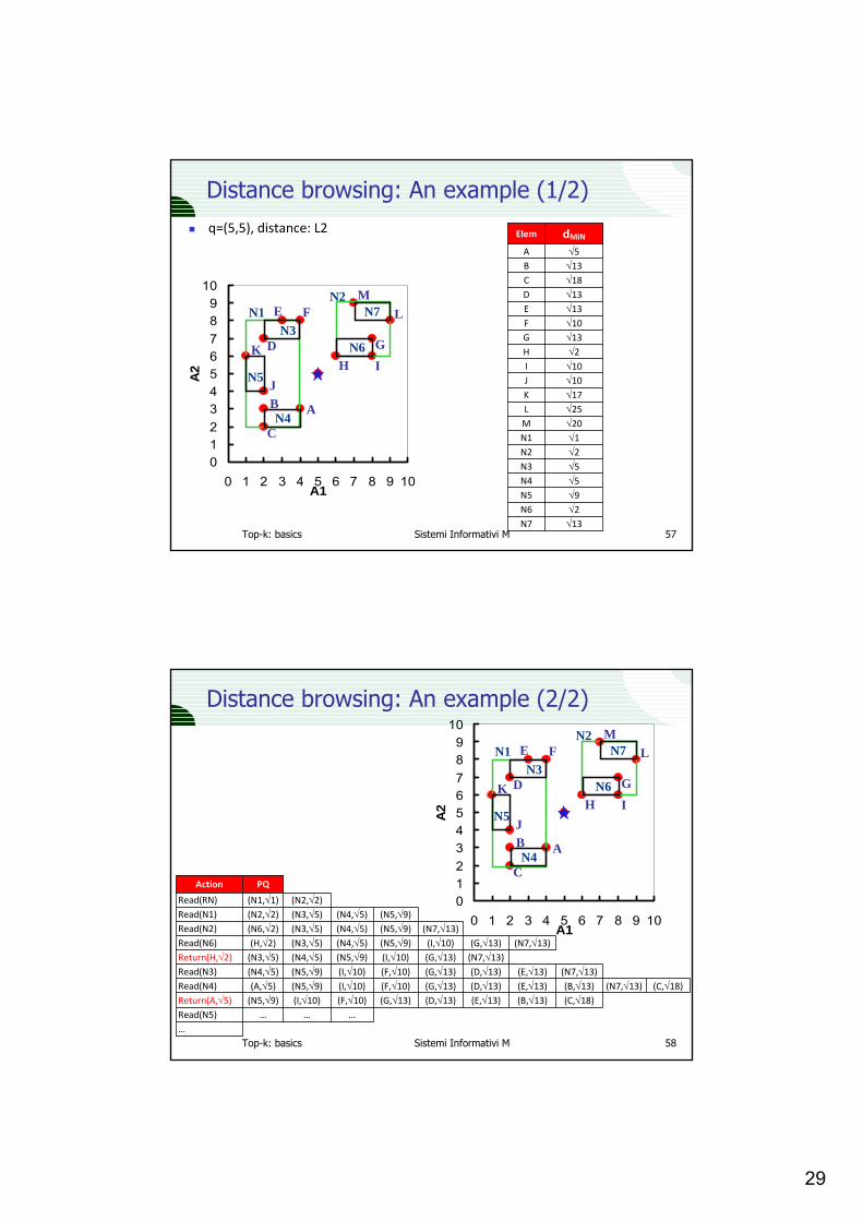
Distance browsing: An example (1/2)q=(5,5), distance: L2
0123456789
10
0 1 2 3 4 5 6 7 8 9 10A1
A2
N1
A
√5N4√9N5√2N6
√13E√10F√13G√2H√10I√10J√17K√25L√20M√1N1√2N2√5N3
√13N7
√13√18√13√5
dMINElem
DCBA
B
C
D
E F
GH I
J
K
LMN2
N3
N4
N5
N6
N7
Top-k: basics Sistemi Informativi M 58
Distance browsing: An example (2/2)
(C,√18)(B,√13)(E,√13)(E,√13)
(N7,√13)
(E,√13)(D,√13)(D,√13)(N7,√13)(G,√13)
(D,√13)(G,√13)(G,√13)(G,√13)(I,√10)(N7,√13)
(G,√13)(F,√10)(F,√10)(I,√10)(N5,√9)(N5,√9)(N5,√9)
(N2,√2)(N1,√1)Read(RN)
(N7,√13)(C,√18)(B,√13)(N7,√13)
…(F,√10)(I,√10)(I,√10)(N5,√9)(N4,√5)(N4,√5)(N4,√5)
…Read(N5)Return(A,√5)Read(N4)Read(N3)Return(H,√2)Read(N6)Read(N2)Read(N1)
Action
(N5,√9)(N4,√5)(N5,√9)(A,√5)(I,√10)(N5,√9)……
(N4,√5)(N3,√5)(N3,√5)(N3,√5)
PQ
(N3,√5)(H,√2)(N6,√2)(N2,√2)
0123456789
10
0 1 2 3 4 5 6 7 8 9 10A1
A2
N1
AB
C
D
E F
GH I
J
K
LMN2
N3
N4
N5
N6
N7

30
Top-k: basics Sistemi Informativi M 59
Indexes as iterators
get_next_NN is just an implementation of the general get_next method for indexes that support incremental k‐NN queriesIn practice, the specific query type (range, k‐NN, incremental k‐NN, etc.), is a parameter passed to the index with the openmethod, after that a simple get_next() suffices
Top-k: basics Sistemi Informativi M 60
Recap
The basic way to process a top‐k selection query is to insert a Top‐Sort operator in the access plan of the query, which saves the overhead of sorting the whole input stream
If the scoring function S is 1‐dimensional, a B+‐tree index on the ranking attribute can be used to efficiently retrieve only the best k tuples
On the other hand, for D‐dim scoring functions an R‐tree based solution is the only way to avoid unnecessary work. In this case the problem amounts to solve a k‐NN query, where the query point q is the “target” of the search (the ideal case) and the distance function d is derived from the scoring function S