01/31/02 (c) 2002, university of wisconsin, cs 559 last time color and color spaces

01/31/02 (C) 2002, UNiversity of Wisconsin, CS 559

Last Time

• Color and Color Spaces


Today

• Image file formats– GIF

– JPEG

• Color Quantization– Uniform

– Populosity

– Median Cut

– Optimization


Image File Formats

• How big is the image?– All files in some way store width and height

• How is the image data formatted?– Is it a black and white image, a grayscale image, a color image, an

indexed color image?– How many bits per pixel?

• What other information?– Color tables, compression codebooks, creator information…


The Simplest File

• Assumes that the color depth is known and agreed on

• Store width, height, and data for every pixel in sequence

• This is how you normally store an image in memory

• Unsigned because width and height are positive, and unsigned char because it is the best type for raw 8 bit data

• Note that you require some implicit scheme for laying out a rectangular array into a linear one

class Image {unsigned int width;unsigned int height;unsigned char *data;

}

3r,g,b

0r

0r,g,b 1r,g,b 2r,g,b

4r,g,b 5r,g,b

8r,g,b7r,g,b6r,g,b

0g 0b 1g1r 1b 2r 2g 2b 3r 3g


Indexed Color

• 24 bits per pixel (8-red, 8-green, 8-blue) are expensive to transmit and store

• It must be possible to represent all those colors, but not in the same image

• Solution: Indexed color– Assume k bits per pixel (typically 8)

– Define a color table containing 2k colors (24 bits per color)

– Store the index into the table for each pixel (so store k bits for each pixel)

– Once common in hardware, now rare (256 color displays)


Indexed Color

Color Table0

1

2

3

4

5

6

7

4 3 0 2

1 7 4 5

3 7 6 5

2 2 1 1

Pixel Data Image

Only makes sense if you have lots of pixels and not many colors


Image Compression

• Indexed color is one form of image compression– Special case of vector quantization

• Alternative 1: Store the image in a simple format and then compress with your favorite compressor– Doesn’t exploit image specific information– Doesn’t exploit perceptual shortcuts

• Two historically common compressed file formats: GIF and JPEG– GIF should now be replaced with PNG, because GIF is patented and

the owner started enforcing the patent


GIF

• Header – Color Table – Image Data – Extensions

• Header gives basic information such as size of image and size of color table

• Color table gives the colors found in the image– Biggest it can be is 256 colors, smallest is 2

• Image data is LZW compressed color indices

• To create a GIF:– Choose colors

– Create an array of color indices

– Compress it with LZW


LZW Compression

• Compresses a stream of “characters”, in GIF case they are 1byte color indices

• Stores the strings encountered in a codebook– When compressing, strings are put in the codebook the second time

they are encountered

– Subsequent encounters replace the string with the code

– Decoding reconstructs codebook on the fly

– Advantage: The code does not need to be transmitted


JPEG

• Multi-stage process intended to get very high compression with controllable quality degradation

• Start with YIQ color– Why? Recall, it’s the

color standard for TV


Discrete Cosine Transform

• A transformation to convert from the spatial to frequency domain – done on 8x8 blocks

• Why? Humans have varying sensitivity to different frequencies, so it is safe to throw some of them away

• Basis functions:


Quantization

• Reduce the number of bits used to store each coefficient by dividing by a given value– If you have an 8 bit number (0-255) and divide it by 8, you get a

number between 0-31 (5 bits = 8 bits – 3 bits)

– Different coefficients are divided by different amounts

– Perceptual issues come in here

• Achieves the greatest compression, but also quality loss

• “Quality” knob controls how much quantization is done


Entropy Coding

• Standard lossless compression on quantized coefficients– Delta encode the DC components

– Run length encode the AC components• Lots of zeros, so store number of zeros then next value

– Huffman code the encodings


Lossless JPEG With Prediction

• Predict what the value of the pixel will be based on neighbors

• Record error from prediction– Mostly error will be near zero

• Huffman encode the error stream

• Variation works really well for fax messages


Color Quantization

• The problem of reducing the number of colors in an image with minimal impact on appearance– Extreme case: 24 bit color to black and white

– Less extreme: 24 bit color to 256 colors, or 256 grays

• Why do we care?

• Sub problems:– Decide which colors to use (if there is a choice)

– Decide which of those each original color maps to


Example (24 bit color)


Quantization Error

• A way of measuring the quality of our approximation

• Define an error for each color, c, in the original image: d(c,c’), where c’ is the color c maps to under the quantization– Common is to use squared distance in RGB space

– Should really use distance in CIE u’,v’ space

• Sum up the error over all the pixels


Uniform Quantization

• Break the color space into uniform cells• Find the cell that each color is in, and map it to the center• Generally does poorly because it fails to capture the

distribution of colors– Some cells may be empty, and are wasted

• Equivalent to dividing each color by some number and taking the integer part– Say your original image is 24 bits color (8 red, 8 green, 8 blue)– Say you have 256 colors available, and you choose to use 8 reds, 8

greens and 4 blues (8 × 8 × 4 = 256 )– Divide original red by 32, green by 32, and blue by 64


Uniform Quantization

• 8 bits per pixel in this image

• Note that it does very poorly on smooth gradients

• Normally the hardest part to get right, because lots of similar colors appear very close together


Populosity Algorithm

• Build a color histogram: count the number of times each color appears

• Choose the n most commonly occurring colors– Typically group colors into small cells first

• Map other colors to the closest chosen color

• Problem: May completely ignore under-represented but important colors


Populosity Algorithm

• 8 bit image, so the most popular 256 colors

• Note that blue wasn’t very popular, so the crystal ball is now the same color as the floor


Median Cut

• Look at distribution of colors

• Recursively:– Find the “longest” dimension (r, g, b are dimensions)

– Choose the median of the long dimension as a color to use

– Split along the median plane, and recurse on both halves

• Works very well in practice

• This algorithm is building a kD-tree, a common form of spatial data structure– Also used in nearest neighbor computations and many other areas of

computer graphics


Median Cut in Action

Original colors in color space

Median in long dimension

Put median color in color table

Recurse


Median Cut

• 8 bit image, so 256 colors

• Now we get the blue

• Median cut works so well because it divides up the color space in the “most useful” way


Optimization Algorithms

• The quantization problem can be phrased as optimization– Find the set of colors and mapping that result in the lowest

quantization error

• Several methods to solve the problem, but of limited use unless the number of colors to be chosen is small– It’s expensive to compute the optimum

– It’s also a poorly behaved optimization


Perceptual Problems

• While a good quantization may get close colors, humans still perceive the quantization

• Biggest problem: Mach bands– The difference between two colors is more pronounced when they

are side by side and the boundary is smooth

– This emphasizes boundaries between colors, even if the color difference is small

– Rough boundaries are “averaged” by our vision system to give smooth variation


Mach Bands in Reality

The floor appears banded


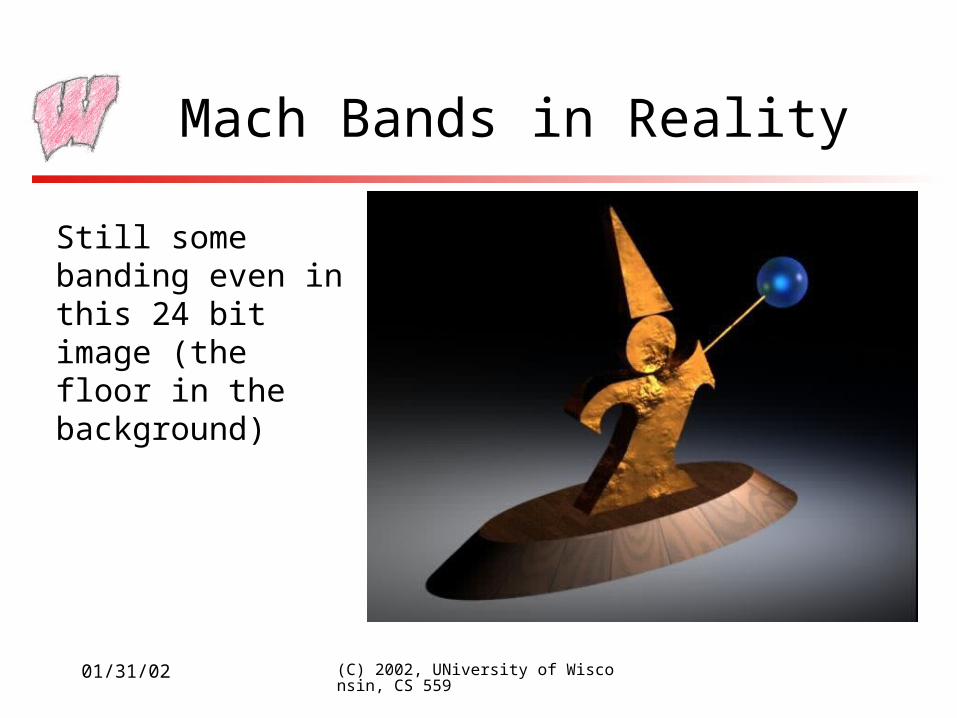
Mach Bands in Reality

Still some banding even in this 24 bit image (the floor in the background)


Mach bands Emphasized

• Note that each bar on the left appears to have color variation across it– Left edge appears darker

than right

• The effect is entirely due to Mach banding


Next Lecture

• How to avoid Mach banding. The solution is dithering

01/31/02 (c) 2002, university of wisconsin, cs 559 last time color and color spaces

Documents