022ampacity.pdf

7/28/2019 022Ampacity.pdf

http://slidepdf.com/reader/full/022ampacitypdf 1/17

Performance of underground power cables under extreme soil

and environmental conditions

A. A. AL-OHALY

King Saud University, P.O.Box 800, Riyadh 11421, Saudi Arabia

ABSTRACT

The use of underground power cables in the Kingdom of Saudi Arabia (KSA) has grown

signi®cantly over the past three decades as a result of urban expansion and increasedinfrastructure activities. Most cable design and operation guidelines are based on

international publications, which use design, soil, and environmental parameters

developed for harsh climates in calculating the cable ampacity. However, in KSA,

extreme soil and environmental conditions exist where the ambient temperature

sometimes exceeds 508C and the very dry soil in the summer produces high thermal

resistance. Under such conditions, the environmental and soil parameters signi®cantly

in¯uence the current-carrying capability of the power cable. In most previous

publications, the eects of such parameters have traditionally been studied individually

with one parameter being varied while all others are ®xed at their respective nominal

values. In this paper, a novel analysis is presented where multi-parameter eects areexamined simultaneously using traditional y-x plots. This new approach has revealed

several important characteristics of the cable performance under design, operation and

environmental parameter changes. The new approach has been applied to a practical

cable system in the Saudi power grid and the results obtained con®rmed the usefulness of

the technique developed.

Keywords: Power systems; Sensitivity analysis, Thermal analysis; Underground

cables.

INTRODUCTION

A common characteristic of modern power transmission and distribution grids

is the extensive use of underground power cables (Neher & McGrath 1957,

Symm 1969). The question of how the power cables are optimized for best

performance has become of utmost importance, especially under the present

conditions which encourage cost savings and high service quality. Signi®cant

design and operating cost reductions could be achieved via optimizing cable

performance under various loading and soil conditions. In this regard, advanced

computer-aided tools for power cable analysis can be used to assist cableengineers in making the right choices regarding cable installation designs and

operating scenarios (El-Kady 1982, Wandmacher 1997).

Kuwait J. Sci. Eng. 30(1) 2003



The use of underground power cables in the Kingdom of Saudi Arabia (KSA)

has grown signi®cantly over the past three decades as a result of urban

expansion and increased infrastructure activities. Most cable design and

operation guidelines are based on international publications which use design,soil, and environmental parameters developed for harsh climates in calculating

the cable ampacity. However, in KSA, extreme soil and environmental

conditions exist where the ambient temperature sometimes exceeds 508C and the

very dry soil in the summer produces high thermal resistance. Under such

conditions, the environmental and soil parameters signi®cantly in¯uence the

current-carrying capability of the power cable. In most previous publications,

the eects of various operation, design, soil and environmental parameters on

the current-carrying capability of the power cable have traditionally been

studied individually with one parameter being varied while all others are ®xed attheir respective nominal values (El-Kady 1984, Bertani et al. 1998).

In this paper, a novel analysis is presented where multi-parameter eects are

examined simultaneously using traditional y-x plots. This has revealed several

important characteristics of cable performance under soil and environmental

parameter changes. The new approach has been applied to a practical cable

system in the Saudi power grid. The results are displayed in multi-parameter

contour graphs, which facilitates examination and interpretation of various

parameter eects on cable ampacity, voltage regulation and losses. The resultsobtained con®rmed the usefulness of the technique.

PROBLEM FORMULATION

The ampacity of cable is limited primarily by the permissible operating

temperature of its insulation. The higher the operating temperature of the

insulation, the greater its allowable ampacity. The temperature at which a

particular cable will operate is aected by ability of the surrounding medium to

dissipate the heat, hence, cable allowable ampacity is aected by ambient

temperature, soil thermal properties and insulation conditions. The presence of

other current-carrying cables in the vicinity increase the "load" ambient

temperature, which decreases the ability of the cable to dissipate heat.

Occasionally, overload conditions may aect cable size. When a cable traverses

more than one raceway, the ampacity of the complete system is the lowest of the

allowable ampacities in each raceway or cable tray, de®ning the "limiting

ampacity".

A key aspect in the computer-aided design of underground power cables is

the computerized evaluation of the cable temperature. Two main approacheshave evolved for the solution of the problem of steady-state and transient

temperature rise calculations of power cables. They dier mainly in how they

298 A. A. Al-Ohaly



formulate the thermal model of the cable system and then solve the resulting set

of mathematical equations.

In the ®rst approach, approximate analytical models are constructed and a

solution scheme is employed based on the traditional work by Neher &

McGrath (1957), which was incorporated and developed further in El-Kady

et al. (1988). In the second approach, numerical methods are applied to

accurately model the cables and their surrounding medium and, then, to solve

the partial dierential equations describing the heat conduction in the soil.

Historically, the analytical methods were developed ®rst with a host of

simplifying assumptions which allow hand computations to be performed. The

most signi®cant of these assumptions are the following:

1. both soil thermal resistivity and diusivity are constant in the external

region surrounding the cable,

2. the soil surface is isothermal, having a pre-speci®ed temperature which

remains constant throughout all calculations, and

3. the cables are located in an in®nite uniform medium of constant thermal

parameters.

Almost all analytical models currently available assume that the system being

examined is composed of identical, equally loaded cables. That is, all cables aresimultaneously carrying the same current. Numerical techniques, such as ®nite

dierence and ®nite element methods, do not require any of these assumptions.

They, however, are much more dicult to perform by cable engineers and,

therefore, have not been a subject of standardization.

The permissible current rating of an ac cable can be derived from the

following expression for temperature rise (Neher & McGrath 1957):

Á I

2

R 0:5W d T 1 I

2

R1 1 W d n T 2 I 2R1 1 2 W d n T 3 T 4: 1

In equation (1), the following terms are de®ned:

I = Current ¯owing in one conductor (A)

Á = Conductor temperature rise above the ambient temperature (8C)

R = Alternating current resistance per unit length of the conductor at

maximum operating temperature (ohm/m)

W d = Dielectric loss per unit length for insulation surrounding the conductor

(W/m)

299Performance of underground power cables under extreme soil and environmental conditions



n = Number of load-carrying conductors in the cable

1 = Ratio of losses in metal sheet to total losses in all cable conductors

2 = Ratio of losses in armouring to total losses in all cable conductors

T 1 = Thermal resistance per unit length between one conductor and sheath

(8C.m/W)

T 2 = Thermal resistance per unit length of sheath-to-armour bedding (8C.m/W)

T 3 = Thermal resistance per unit length of the external serving of the cable

(8C.m/W)

T 4 = Thermal resistance per unit length of the medium around the cable

(8

C.m/W)Equation (1) is the basis of three types of steady-state computations which

can be performed by the cable design engineer, namely: i) Ampacity calculations

of equally loaded identical cables, ii) Ampacity calculations of unequally loaded

or dissimilar cables, and iii) Temperature calculations of a group of cables. In

cases (i) and (ii) the maximum conductor temperature values must be speci®ed,

while in case (iii) the current loading of all cables in the study must be known.

For calculations of ampacity of unequally loaded cables in case (ii), a reference

cable must be de®ned and the algorithm will calculate the ampacities of various

cables such that the reference cable reaches its maximum operating temperature,and currents in remaining cables will be the highest possible without exceeding

their thermal ratings.

In the cases where some parameters in equation (1) are temperature and/or

current dependent, the computational procedure is an iterative one. The values

of thermal resistances T1, T2, T3 and T4 depend on the cable type, lay-out and

dimensions. Analytical expressions to calculate these thermal resistances for

various cable types are available in the literature (Neher & McGrath 1957,

Symm 1969).

In most computer-aided cable design studies, the engineer would typically

perform numerous steady-state temperature computations for many cable

design scenarios (dierent cable dimensions, conductor and insulation materials,

etc.) and select the most appropriate design which meets all thermal loading

requirements at the minimum cost.

Voltage regulation is also important in assessing the performance of

underground cables. The voltage drop (VD) is calculated using the approximate

formula:

VD I R os I X sin 2a

300 A. A. Al-Ohaly



In equation (2a)

VD = voltage drop in volts per 1000 ft. line to neutral.

I = line current in amperes.

R = line resistance in ohm per 1000 ft.

X = line inductive reactance in ohm per 1000 ft.

os = load power factor.

sin = load reactive factor.

The reactance X is given by

X = 2 f 0:1404 logr=s 0:0153 Â 10À3 2bwhere

f = supply frequency in hertz.

r = radius of conductor in inches.

s = equivalent spacing of conductors between centers in inches for a

three conductor triangular con®guration.

=

ABC 3p s 3a= A for equilateral triangle (3b)

= 1.123 A for right angle triangle (3c)

= 1.26 A for symmetrical ̄ at (3d)

where

A; B; C = distance between adjacent conductors in inches in triangular

con®guration.

PRACTICAL APPLICATIONS

Description of cable system

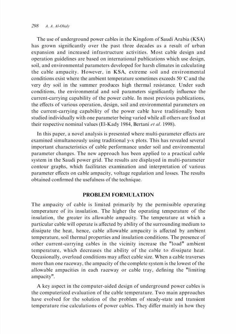
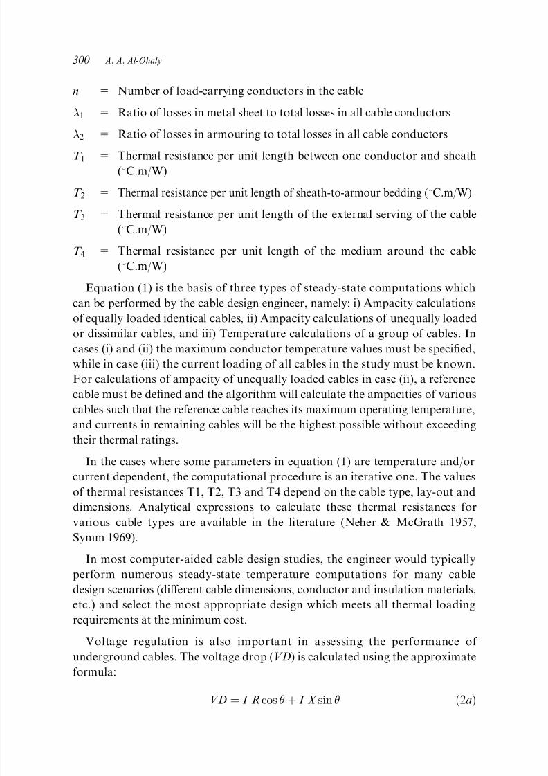
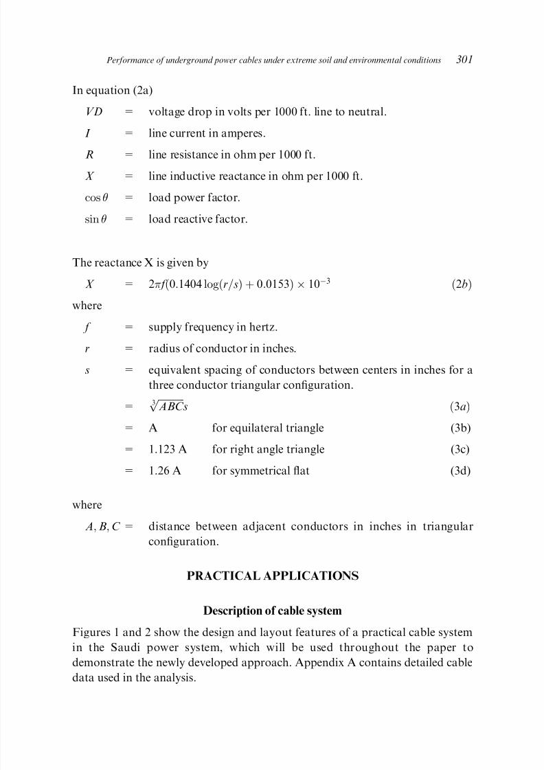
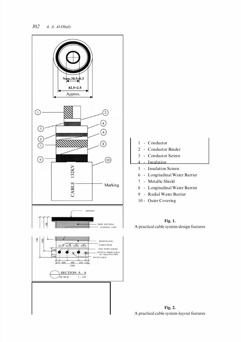
Figures 1 and 2 show the design and layout features of a practical cable system

in the Saudi power system, which will be used throughout the paper to

demonstrate the newly developed approach. Appendix A contains detailed cable

data used in the analysis.




1 - Conductor

2 - Conductor Binder

3 - Conductor Screen

4 - Insulation

5 - Insulation Screen

6 - Longitudinal Water Barrier

7 - Metallic Shield

8 - Longitudinal Water Barrier

9 - Radial Water Barrier

10 - Outer Covering

Fig. 1.

A practical cable system-design features

Fig. 2.

A practical cable system-layout features

302 A. A. Al-Ohaly



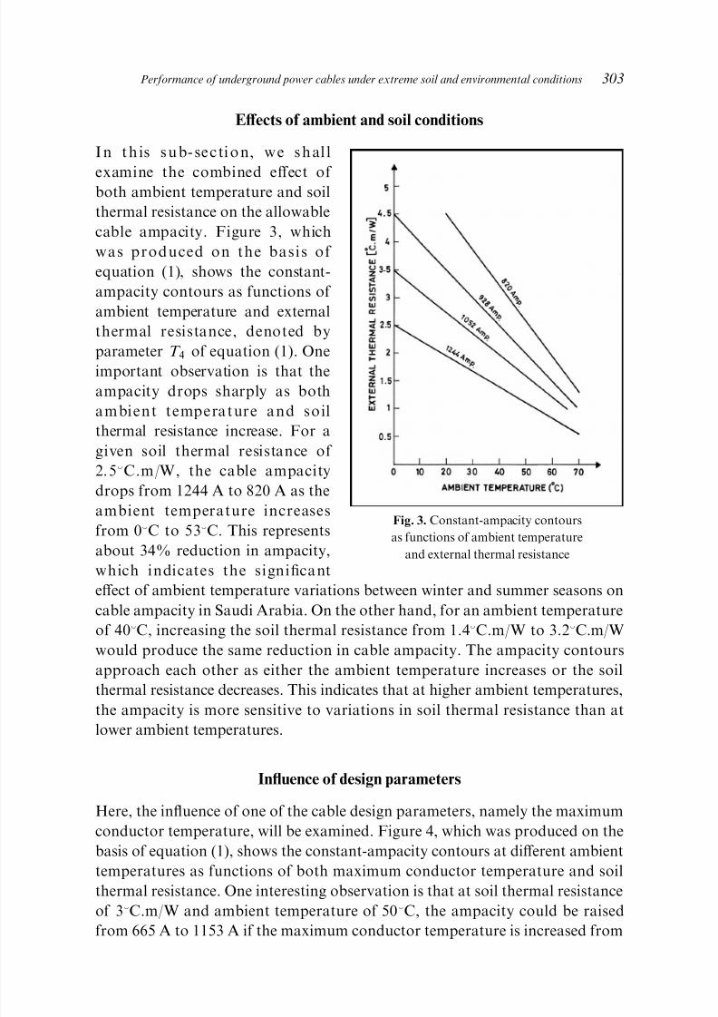
Eects of ambient and soil conditions

I n t h is s u b- se c ti o n, w e s h al l

examine the combined eect of both ambient temperature and soil

thermal resistance on the allowable

cable ampacity. Figure 3, which

was produced on the basis of

equation (1), shows the constant-

ampacity contours as functions of

ambient temperature and external

thermal resistance, denoted by

parameter T 4 of equation (1). Oneimportant observation is that the

ampacity drops sharply as both

ambient temperature and soil

thermal resistance increase. For a

given soil thermal resistance of

2.58C.m/W, the cable ampacity

drops from 1244 A to 820 A as the

ambient temperature increases

from 08C to 53

8C. This represents

about 34% reduction in ampacity,

which indicates the signi®cant

eect of ambient temperature variations between winter and summer seasons on

cable ampacity in Saudi Arabia. On the other hand, for an ambient temperature

of 408C, increasing the soil thermal resistance from 1.48C.m/W to 3.28C.m/W

would produce the same reduction in cable ampacity. The ampacity contours

approach each other as either the ambient temperature increases or the soil

thermal resistance decreases. This indicates that at higher ambient temperatures,

the ampacity is more sensitive to variations in soil thermal resistance than atlower ambient temperatures.

In¯uence of design parameters

Here, the in¯uence of one of the cable design parameters, namely the maximum

conductor temperature, will be examined. Figure 4, which was produced on the

basis of equation (1), shows the constant-ampacity contours at dierent ambient

temperatures as functions of both maximum conductor temperature and soil

thermal resistance. One interesting observation is that at soil thermal resistanceof 38C.m/W and ambient temperature of 508C, the ampacity could be raised

from 665 A to 1153 A if the maximum conductor temperature is increased from

Fig. 3. Constant-ampacity contours

as functions of ambient temperatureand external thermal resistance




838C to 1208C. The same increase in ampacity could be obtained for a given

maximum conductor temperature of 1008C if the soil thermal resistance is

lowered from 4.28C.m/W to 2.28C.m/W at the same ambient temperature of

508C.

Fig. 4. Constant-ampacity contours at dierent ambient temperatures as functions

of both maximum conductor temperature and soil thermal resistance

In¯uence of operating parameters

Examples of important cable operating parameters are the loading power-factor

and voltage regulation. Figure 5, which was produced on the basis of equation

(1), shows the constant voltage regulation contours as functions of both ambient

temperature and power-factor, when the cable is loaded to its ampacity level. It

is clear that the relationships are non-linear and that, for a given loading power-

factor, higher voltage regulation is obtained as lower ambient temperature

decreases. Another interesting observation is that, for a given value of ambient

temperature, a speci®ed voltage regulation value can be obtained at more than

one power-factor level. For example, at an ambient temperature of 158C, avoltage regulation of 4.68% can be obtained at both 0.4 and 0.75 lagging power-

factors.

304 A. A. Al-Ohaly



Fig. 5. Constant voltage regulation contours as functions

of both ambient temperature and power-factor

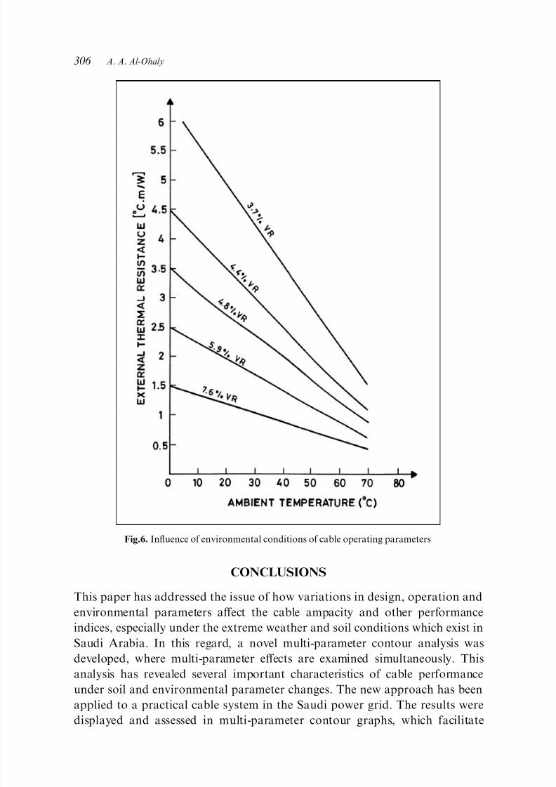
Combined eect of operating and environmental parameters

Figure 6, which was produced on the basis of equation (1), demonstrates how

the cable operating parameters are in¯uenced by environmental conditions. Itshows the constant voltage regulation contours as functions of both ambient

temperature and external thermal resistance. The curves are almost straight lines

of varying slopes. The sensitivity of voltage regulation with respect to external

thermal resistance increases at higher ambient temperature values. In addition,

voltage regulation increases as either or both ambient temperature and external

thermal resistance decrease. For example, at an ambient temperature of 308C,

the voltage regulation increases from 4.4% to 7.6% if the external thermal

resistance decreases from 38C.m/W to 18C.m/W.




Fig.6. In¯uence of environmental conditions of cable operating parameters

CONCLUSIONS

This paper has addressed the issue of how variations in design, operation and

environmental parameters aect the cable ampacity and other performance

indices, especially under the extreme weather and soil conditions which exist in

Saudi Arabia. In this regard, a novel multi-parameter contour analysis was

developed, where multi-parameter eects are examined simultaneously. This

analysis has revealed several important characteristics of cable performance

under soil and environmental parameter changes. The new approach has beenapplied to a practical cable system in the Saudi power grid. The results were

displayed and assessed in multi-parameter contour graphs, which facilitate

306 A. A. Al-Ohaly



examination and interpretation of various parameter eects on cable ampacity,

voltage regulation and losses. The results obtained con®rmed the usefulness of

the developed multi-parameter contour graphs in identifying the relative eects

of various design and environmental parameters on cable ampacity.

REFERENCES

Bertani, E., Bonfanti, I., Bosotti, O., Giornelli, F., Valagussa, C. & Kai, S.L. 1998. CESI experiencein the ®eld of power cables. Proceedings of International Conference on Power System

Technology, pp. 181-187.

El-Kady, M.A. 1982. Optimization of power cable and thermal back®ll con®gurations. IEEE

Transactions on Power Apparatus and Systems 101: 4681-4688.

El-Kady, M.A. 1984. Calculation of the sensitivity of power cable ampacity to variations of design

and environmental parameters, IEEE Transactions on Power Apparatus and Systems 103:2043-2050.

El-Kady, M.A., Motlis, J., Anders, G. & Horrocks, D.J. 1988. Modi®ed values for geometric factor

of external thermal resistance of cables in duct banks. IEEE Transactions on Power Delivery3(4): 1303-1309.

Neher, J.H. & McGrath, M.H. 1957. The calculation of the temperature rise and load capability of

cable systems. AIEE Transactions (Power Apparatus and Systems) 76(3): 752-772.

Symm, G.T. 1969. External thermal resistance of buried cables and throughs. Proceedings IEEE

116: 1695-1698.

Wandmacher, R.A. 1997. New terminations for distribution-class shielded power cables, Part 1:

Contributions. Proceedings 14th International Conference and Exhibition on Electricity

Distribution 3: 38/1-38/5.

Submitted : 29/9/2001

Revised : 22/10/2002

Accepted : 11/1/2003

307 Performance of underground power cables under extreme soil and environmental conditions



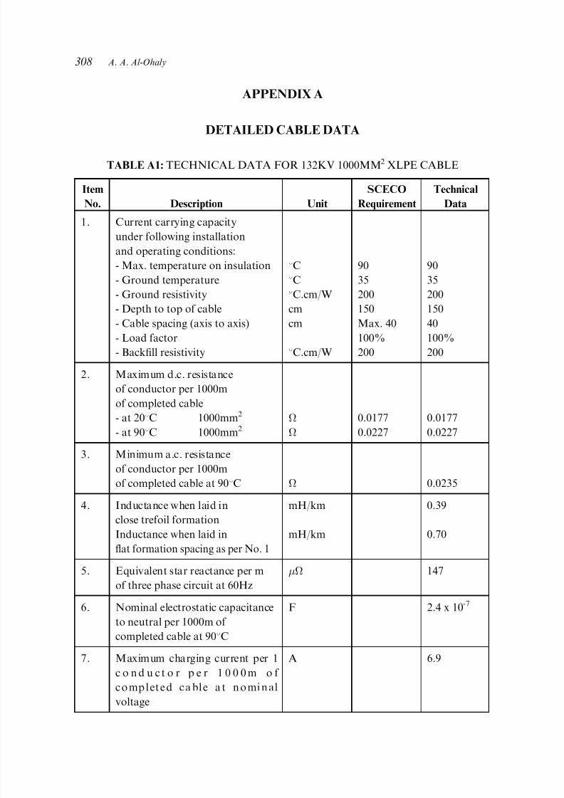
APPENDIX A

DETAILED CABLE DATA

TABLE A1: TECHNICAL DATA FOR 132KV 1000MM2 XLPE CABLE

Item

No. Description Unit

SCECO

Requirement

Technical

Data

1. Current carrying capacity

under following installation

and operating conditions:

- Max. temperature on insulation

- Ground temperature- Ground resistivity

- Depth to top of cable

- Cable spacing (axis to axis)

- Load factor

- Back®ll resistivity

8C

8C8C.cm/W

cm

cm

8C.cm/W

90

35200

150

Max. 40

100%

200

90

35200

150

40

100%

200

2. Maximum d.c. resistance

of conductor per 1000m

of completed cable

- at 208C 1000mm

2

- at 908C 1000mm2

0.01770.0227

0.01770.0227

3. Minimum a.c. resistance

of conductor per 1000m

of completed cable at 908C 0.0235

4. Inductance when laid in

close trefoil formation

Inductance when laid in

¯at formation spacing as per No. 1

mH/km

mH/km

0.39

0.70

5. Equivalent star reactance per m

of three phase circuit at 60Hz

147

6. Nominal electrostatic capacitance

to neutral per 1000m of

completed cable at 908C

F 2.4 x 10-7

7. Maximum charging current per 1

c o n d u c t o r p e r 1 0 0 0 m o f

c o mp l et e d c a bl e a t n o mi n al

voltage

A 6.9

308 A. A. Al-Ohaly



TABLE A1: TECHNICAL DATA FOR 132KV 1000MM2 XLPE CABLE (cont'd)

Item


SCECO

Requirement

Technical

Data

8. Maximum dielectric loss of cable

per m of 3-phase circuit when laid

direct in the ground at nominal

voltage, nominal frequency at

908C

W 1.6

9. Sheath loss of completed cable per

m of 3-phase circuit at nominal

voltage, nominal frequency at

current rating given in Item 1

above

W 3.7

10. Total losses when cable loaded as

in item 1 above

kW/km 53.8

11. Maximum value of tangent of

dielectric loss angle of cable at

nominal frequency of 60Hz

- at 208C at nominal voltage

- at 908C at nominal voltage

- at 208C at 200% of nominal voltage

0.1%

0.1%

0.1%

12. Maximum change in tangent of

dielectric loss angle between

n o mi n al v o lt a ge a n d 2 0 0%

nominal voltage at 208C 0.05%

13. Relative dielectric constant at

208C

2.5

14. Average electric stress kV/km 4.3

15. Conductor short circuit current

carrying capacity for 1 second

when cable loaded as in Item 1

before short circuit, and ®nal

conductor temperature of 2508C

kA Min. 40 144

16. Minimum insulation resistance at

208C

M/km 2650

17. Minimum insulation resistance at

908C

M/km 1.06




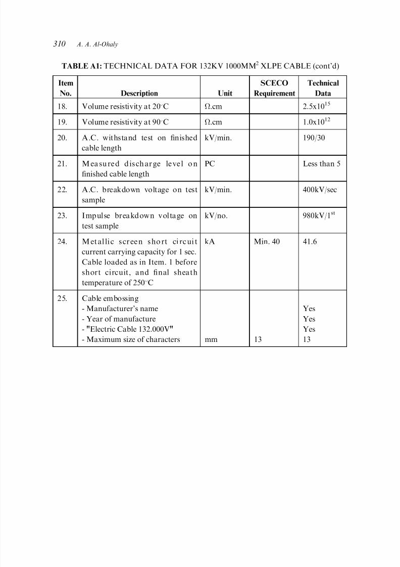
TABLE A1: TECHNICAL DATA FOR 132KV 1000MM2 XLPE CABLE (cont'd)

Item


SCECO

Requirement

Technical

Data

18. Volume resistivity at 208C .cm 2.5x1015

19. Volume resistivity at 908C .cm 1.0x1012

20. A.C. withstand test on ®nished

cable length

kV/min. 190/30

21. M ea su re d d is ch ar ge le ve l o n

®nished cable length

PC Less than 5

22. A.C. breakdown voltage on test

sample

kV/min. 400kV/sec

23. Impulse breakdown voltage on

test sample

kV/no. 980kV/1st

24. M et al li c s cr ee n s ho rt ci rc ui t

current carrying capacity for 1 sec.

Cable loaded as in Item. 1 before

short circuit, and ®nal sheath

temperature of 2508C

kA Min. 40 41.6

25. Cable embossing- Manufacturer's name

- Year of manufacture

- "Electric Cable 132.000V"

- Maximum size of characters mm 13

Yes

Yes

Yes

13

310 A. A. Al-Ohaly



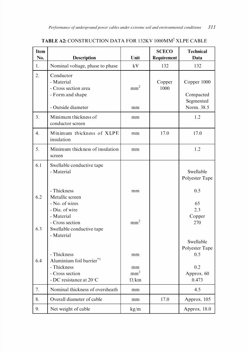
TABLE A2: CONSTRUCTION DATA FOR 132KV 1000MM2 XLPE CABLE

Item


SCECO

Requirement

Technical

Data

1. Nominal voltage, phase to phase kV 132 132

2. Conductor

- Material

- Cross section area

- Form and shape

- Outside diameter

mm2

mm

Copper

1000

Copper 1000

Compacted

Segmented

Norm. 38.5

3. Minimum thickness of

conductor screen

mm 1.2

4. Minimum thickness of XLPE

insulation

mm 17.0 17.0

5. Minimum thickness of insulation

screen

mm 1.2

6.1

6.2

6.3

6.4

Swellable conductive tape

- Material

- Thickness

Metallic screen

- No. of wires

- Dia. of wire

- Material

- Cross section

Swellable conductive tape

- Material

- Thickness

Aluminium foil barrier*1

- Thickness

- Cross section

- DC resistance at 208C

mm

mm2

mm

mm

mm2

/km

Swellable

Polyester Tape

0.5

65

2.3

Copper

270

Swellable

Polyester Tape

0.5

0.2

Approx. 60

0.473

7. Nominal thickness of oversheath mm 4.5

8. Overall diameter of cable mm 17.0 Approx. 105

9. Net weight of cable kg/m Approx. 18.0




TABLE A2: CONSTRUCTION DATA FOR 132KV 1000MM2 XLPE CABLE (cont'd)

Item


SCECO

Requirement

Technical

Data

10. Nominal drum length m 500*2

11. Minimum radius of bend

- Laid direct or in air

- Laid in ducts

mm

mm

2.0

2.0

312 A. A. Al-Ohaly



COGA v9 <; JG y t ( iG }Q \ + ? p, c{ cQ haG y A Q <? hG y = + 8 ? G y t 9 S + ?

f = O G y J } + O f = O G y( $9 HG y g ( $ z ,

F9 | g ? G y } z x S g ( OU.H.800G yQ *9 V11421-G y } } z w ? G y g Q < + ? G y T g ( O *?

L; Y?

y t O @ " 9 |) G S A M O Ge v9 <; JG y t ( iG}Q \ + ? p, G y } } z w ? G y g Q < + ? G y T g ( O *? < W w { hG Sh L; dG y g t ( OG y D ; C? G y } 9 \ + ? hP yx ! A + G ? y z A ( Sh G y J ] Q jhG: | A O GOG y g } Q G !, hGRO *9 O

G y = " ) G y A J A + ? @ = g 9 k

yP yx . y t O C Y = K @ Z } + ~ h @ W j + { G y w 9 <; J * M ] h : f A = 9 QGJhC S9 y + > f9 y } + ? @ T A M O e | g 9 * + Q | A j + Q IPGJ f; s? <9 y A Q <? hG y = + 8 ? p, c{ cQ ha s9 S + ? y z g ( G |{ G y } " 9 L + ? hG y G ( *? hOQ F9 JG y J Q GQI |# C F{ | g Q p? |O i @ J } { G y w 9 <; J

y z A + 9 QGJG y w % Q <9 F + ? G y A , @ T Q j p + % 9 .h |# G y } g Q haCf p, G y } } z w ? G y g Q < + ? G y T g ( O *? cQ ha p, i9 *? G y W O I |# I + E | w ( !9 JG y A Q <? hC I( GdG y = + 8 ? EP p, p Z { G y Z + r @R OGO

G y A Q <? F q 9 p9 k

h @ Z { OQ F9 JG y J Q GQIE y) IO hO50OQ F? | 8 ( *? G} |Q G yP j @R OGO | g & | t 9 h |? G y w 9 <; J yO Q F? v = + Q I.h <9 y a = h p{ !& ! A + G ? y A z x G y d Q ha p{ f S( AG y A Q <? hG y } " 9 N *| CQ Gf <; Vx f z ) | t O QIG y A J } { y A z x G y w 9 <; J y z A + 9 QGJG y A , @ } Q < % 9 .h <9 y " d Q y z O QG S9 JG y J 9 y + ? ! G O Cf @ z x G y d Q ha sO OQ SB v{ f z ) IO IhC LP J p, G: f A = 9 Q < W w { G ! q Q GOj | } 9 F g z % 9 s9 YQ I p, G y " A 9 FH G y A , @( Y z B E y + % 9 .h y g { $P G |9 IO G <9 y = 9 IE E y) G y A g 9 |{ |h @ z x G y d Q hahG y } g 9 * + Q < W w { F } 9 f, h p, B fhG IO h |# C~ fQ \ % 9 p, C S z ( H i + Q | T = ( b |# I + E G y A J z + { hG: S A " A 9 F9 J | T A M O |9

k p, P yx

Q S( |9 k

hC V w 9 : k < + 9 ! + ? | g Q h p? hhG \ J ? .h y t O C <9 f $P GG} S z ( HG y } t A Q M L Z 9 F[

| A g O OI}OGAG y w 9 <; J p, c{ cQ ha | A = 9 * " ? |# I + E G y A Z } + ~ hG y A W j + { hG y } A j + Q GJG y = + 8 + ? hG y } " 9 L + ? .h y t O @~ @ a = + u $P GG} S z ( H f z ) | " d ( |? |# G y w 9 <; J @ W w { FR AG

k

|# G y " d 9 eG y W 9 |{ y z W = w 9 JG y w % Q <9 F + ? p, G y } } z w ? G y g Q < + ? G y T g ( O *? ,h y t O C *O JG y " A 9 FH

G y A , @~ G y A ( Y{ E y + % 9 |O i p g 9 y + ? h FO hi $P GG} S z ( HG y } a ( Q.


022ampacity.pdf

Documents