02sep randall
DESCRIPTION
navalTRANSCRIPT
7/18/2019 02Sep Randall
http://slidepdf.com/reader/full/02sep-randall 1/112
NAVAL POSTGRADUATE SCHOOL
Monterey, California
THESIS
Approved for public release; distribution is unlimited
FLAPPING-WING PROPULSION AS A MEANS OF DRAG
REDUCTION FOR LIGHT SAILPLANES
by
Brian H. Randall
September 2002
Thesis Advisor: K. D. Jones
Second Reader: M. F. Platzer

7/18/2019 02Sep Randall
http://slidepdf.com/reader/full/02sep-randall 2/112
THIS PAGE INTENTIONALLY LEFT BLANK
7/18/2019 02Sep Randall
http://slidepdf.com/reader/full/02sep-randall 3/112
i
REPORT DOCUMENTATION PAGE Form Approved OMB No. 0704-0188
Public reporting burden for this collection of information is es timated to average 1 hour per response, including
the time for reviewing instruction, searching existing data sources, gathering and maintaining the data needed, and
completing and reviewing the collection of information. Send comments regarding this burden estimate or any
other aspect of this collection of information, including suggestions for reducing this burden, to Washington
headquarters Services, Directorate for Information Operations and Reports, 1215 Jefferson Davis Highway, Suite
1204, Arlington, VA 22202-4302, and to the Office of Management and Budget, Paperwork Reduction Project(0704-0188) Washington DC 20503.
1. AGENCY USE ONLY (Leave blank) 2. REPORT DATE
September 2002
3. REPORT TYPE AND DATES COVERED
Master’s Thesis
4. TITLE AND SUBTITLE:
Flapping-wing Propulsion as a Means of Drag Reduction forLight Sailplanes
6. AUTHOR(S) Randall, Brian H.
5. FUNDING NUMBERS
7. PERFORMING ORGANIZATION NAME(S) AND ADDRESS(ES)
Naval Postgraduate School
Monterey, CA 93943-5000
8. PERFORMING
ORGANIZATION REPORT
NUMBER
9. SPONSORING /MONITORING AGENCY NAME(S) AND ADDRESS(ES) N/A
10. SPONSORING/MONITORINGAGENCY REPORT NUMBER
11. SUPPLEMENTARY NOTES The views expressed in this thesis are those of the author and do not reflect the official
policy or position of the Department of Defense or the U.S. Government.
12a. DISTRIBUTION / AVAILABILITY STATEMENT
Approved for public release; distribution is unlimited
12b. DISTRIBUTION CODE
A
13. ABSTRACT (maximum 200 words)
In this paper, flapping-wing propulsion as a means of drag reduction for light sailplanes is
investigated numerically. The feasibility of markedly improving minimum sink and L/Dmax performance parameters in light sailplanes by flapping their flexible, high aspect ratio wings at
their natural frequencies is considered. Two propulsive systems are explored: a human-
powered system that is used to partially offset airframe drag, and a sustainer system that usesan electric motor with sufficient power for limited climb rates. A numerical analysis is
conducted using a strip-theory approach with UPOT (Unsteady Potential code) data. Thrustand power coefficients are computed for 2-D sections. 3-D spanwise load factors are applied to
calculate total wing thrust production and power consumption. The results show thattheoretical drag reduction in excess of 20%, and improvements of minimum sink by 24% are possible with a human-powered flapping system.
15. NUMBER OF
PAGES 112
14. SUBJECT TERMS
Flapping-Wing Propulsion, Drag-Reduction, Light Sailplanes
16. PRICE CODE
17. SECURITY
CLASSIFICATION OFREPORT
Unclassified
18. SECURITY
CLASSIFICATION OF THISPAGE
Unclassified
19. SECURITY
CLASSIFICATION OFABSTRACT
Unclassified
20. LIMITATION
OF ABSTRACT
UL
NSN 7540-01-280-5500 Standard Form 298 (Rev. 2-89)
Prescribed by ANSI Std. 239-18

7/18/2019 02Sep Randall
http://slidepdf.com/reader/full/02sep-randall 4/112
ii
THIS PAGE INTENTIONALLY LEFT BLANK
7/18/2019 02Sep Randall
http://slidepdf.com/reader/full/02sep-randall 5/112
iii
Approved for public release; distribution is unlimited
FLAPPING-WING PROPULSION AS A MEANS OF DRAG REDUCTION FOR
LIGHT SAILPLANES
Brian H. Randall
Lieutenant, United States NavyB.S., United States Naval Academy, 1994
Submitted in partial fulfillment of the
requirements for the degree of
MASTER OF SCIENCE IN AERONAUTICAL ENGINEERING
from the
NAVAL POSTGRADUATE SCHOOLSeptember 2002
Author: Brian H. Randall
Approved by: Kevin D. Jones
Thesis Advisor
Max F. PlatzerSecond Reader/Co-Advisor
Max F. Platzer
Chairman, Department of Aeronautics and Astronautics

7/18/2019 02Sep Randall
http://slidepdf.com/reader/full/02sep-randall 6/112
i
THIS PAGE INTENTIONALLY LEFT BLANK
7/18/2019 02Sep Randall
http://slidepdf.com/reader/full/02sep-randall 7/112
v
ABSTRACT
In this paper, flapping-wing propulsion as a means of drag reduction for light
sailplanes is investigated numerically. The feasibility of markedly improving minimum
sink and L/Dmax performance parameters in light sailplanes by flapping their flexible,
high aspect ratio wings at their natural frequencies is considered. Two propulsive
systems are explored: a human-powered system that is used to partially offset airframe
drag, and a sustainer system that uses an electric motor with sufficient power for limited
climb rates. A numerical analysis is conducted using a strip-theory approach with UPOT
(Unsteady Potential code) data. Thrust and power coefficients are computed for 2-D
sections. 3-D spanwise load factors are applied to calculate total wing thrust production
and power consumption. The results show that theoretical drag reduction in excess of
20% and improvements of minimum sink by 24% are possible with a human-powered
flapping system.

7/18/2019 02Sep Randall
http://slidepdf.com/reader/full/02sep-randall 8/112
vi
THIS PAGE INTENTIONALLY LEFT BLANK
7/18/2019 02Sep Randall
http://slidepdf.com/reader/full/02sep-randall 9/112
vii
TABLE OF CONTENTS
I. INTRODUCTION .......................................................................................................1
A. OVERVIEW.....................................................................................................1 B. FLAPPING-WING PROPULSION...............................................................1
C. HIGH PERFORMANCE SAILPLANES......................................................3 1. Improving Existing Aircraft ...............................................................4
2. Reducing the Power Requirement .....................................................5 3. Existing Sustainer Sailplanes..............................................................6 4. Ultralight Sailplanes............................................................................9
5. Flapping Mechanism.........................................................................12 a. Human-Powered System......................................................... 15
b. Sustainer System.....................................................................16
II. NUMERICAL ANALYSIS.......................................................................................17 A. STRIP-THEORY APPROACH ...................................................................17
B. 2-D SOLUTION METHOD..........................................................................19 C. 3-D CORRECTIONS ....................................................................................24
D. VALIDATION ...............................................................................................28
III. RESULTS ...................................................................................................................31 A. IDENTIFYING TRENDS.............................................................................31
B. CONSTRAINTS ............................................................................................34 1. Human-Powered SparrowHawk Results..........................................36
2. Human-Powered L ight Hawk Results ..............................................41 3. Sustainer Results................................................................................47
IV. CONCLUSIONS........................................................................................................ 53
V. RECOMMENDATIONS ..........................................................................................55
APPENDIX A. SAILPLANE SPREADSHEET.................................................................57
APPENDIX B. SCHEMPP-HIRTH SUSTAINERS.........................................................59
APPENDIX C. FAR PART 103 REGULATION ..............................................................63
APPENDIX D. MOTORGLIDER AND SUSTAINER SPREADSHEET.......................65
APPENDIX E. NUMERICAL ANALYSIS VALIDATION CODE................................67
APPENDIX F. EXAMPLE OF TREND FINDING CODE (1ST OF 3): FLAPPING
ANGLE AND VELOCITY VARIATION FOR USER-DEFINEDFLAPPING FREQUENCY.......................................................................................71
APPENDIX G. CONSTRAINING CODE 1: HUMAN-POWERED
SPARROWHAWK ....................................................................................................77
APPENDIX H. CONSTRAINING CODE 2: HUMAN-POWERED LIGHT
HAWK/ LIGHT HAWK-BASED SUSTAINER .................................................... 83

7/18/2019 02Sep Randall
http://slidepdf.com/reader/full/02sep-randall 10/112
viii
APPENDIX I. POWER FUNCTION CALLED BY CONSTRAINING CODES ..........89
APPENDIX J. THRUST FUNCTION CALLED BY CONSTRAINING CODES ........91
LIST OF REFERENCES...................................................................................................... 93
INITIAL DISTRIBUTION LIST.........................................................................................95

7/18/2019 02Sep Randall
http://slidepdf.com/reader/full/02sep-randall 11/112
ix
LIST OF SYMBOLS
AR aspect ratio, b2 /S
b effective wing span
b/2 half span
bhp brake horsepower
c chord length
Cd drag coefficient
Cl lift coefficient
Cr root chord
Ct tip chord
f oscillation frequency in Hz
h plunge amplitude in terms of c
k reduced frequency, 2π fc/U
L/D lift to drag ratio, Cl/Cd
M mass
S wing area, bc
t time
U velocity in m/s
w weight in kg
W Watts power
y(t) vertical displacement in terms of c
∆ y plunge displacement in terms of c
α angle of attack in degrees
β angle of bank in degrees
φ flapping angle in degrees
η propulsive efficiency
λ taper ratio

7/18/2019 02Sep Randall
http://slidepdf.com/reader/full/02sep-randall 12/112
x
THIS PAGE INTENTIONALLY LEFT BLANK
7/18/2019 02Sep Randall
http://slidepdf.com/reader/full/02sep-randall 13/112
xi
LIST OF FIGURES
Figure 1. Thrust Production of Purely Plunging Airfoil ...................................................3Figure 2. Natural High Performance Sailplane Wing Deflection .....................................3
Figure 3. 1st Bending Mode Flapping ...............................................................................4Figure 4. Power Required vs. Velocity.............................................................................6
Figure 5. Sustainer-Equipped Duo Discus Sailplane ........................................................7Figure 6. 2 Views of Deployed Sustainer Systems ...........................................................8Figure 7. SparrowHawk Ultralight Sailplane ..................................................................10
Figure 8. Light Hawk Ultralight Sailplane ......................................................................11Figure 9. L/D vs. Velocity for Sparrowhawk and Light Hawk .......................................12
Figure 10. Cantilever with Point Mass.............................................................................. 13Figure 11. Spar Anchoring Point Movement ....................................................................14
Figure 12. Chain-driven Pedal System.............................................................................. 15Figure 13. Fuselage Cross Section....................................................................................16Figure 14. Modeled Semi Span Flapping (left) vs. Actual Flapping (right) .....................17
Figure 15. Elliptical Lift Distribution ...............................................................................18Figure 16. Half Span Dimensions of Interest ....................................................................18Figure 17. Strip-theory Segmentation for Flapping-wing.................................................19
Figure 18. Time Averaged Thrust Coefficient vs. Reduced Frequency ...........................21Figure 19. Airfoil Thickness vs. Thrust Coefficient .........................................................22
Figure 20. Airfoil Camber vs. Thrust Coefficient .............................................................23Figure 21. Purely Plunging Airfoil UPOT Screen Image ................................................. 24Figure 22. Propulsive Efficiency vs. Reduced Frequency................................................25
Figure 23. Straight Plunge vs. Bird-flapping Motions ...................................................... 25Figure 24. Normalized Power Coefficient Semi-span Distribution..................................26
Figure 25. Normalized Thrust Coefficient Semi-span Distribution..................................27Figure 26. Thrust Coefficient vs. Semi-span Position .................................................... 28Figure 27. Validation code vs. CMARC Data for Cp ....................................................... 29
Figure 28. Validation code vs. CMARC Data for Ct........................................................30Figure 29. Sink-rate Contour for Varying Velocity and Flapping Angle .........................31
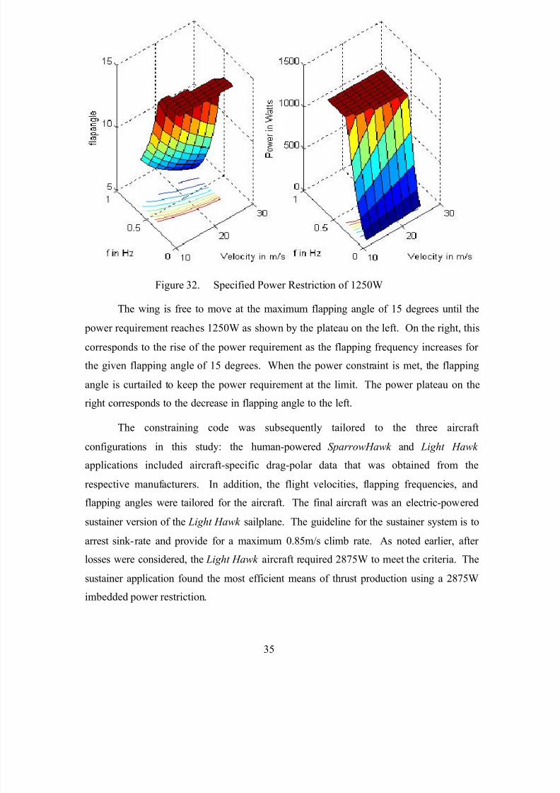
Figure 30. Thrust Plots for Varying Flapping Angles and Frequencies ...........................32Figure 31. Sink-rate Contour for Varying Velocity and Frequency .................................33Figure 32. Specified Power Restriction of 1250W ...........................................................35
Figure 33. SparrowHawk Thrust Production....................................................................36
Figure 34. SparrowHawk Net Drag ..................................................................................37Figure 35. SparrowHawk expanded L/D vs. Velocity......................................................38Figure 36. SparrowHawk Sink Rate..................................................................................39Figure 37. SparrowHawk Flapping Angle Variation........................................................40
Figure 38. SparrowHawk Propulsive Efficiency Contour ................................................ 41Figure 39. Light Hawk Thrust Production.........................................................................42
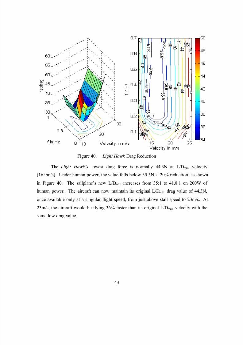
Figure 40. Light Hawk Drag Reduction............................................................................43

7/18/2019 02Sep Randall
http://slidepdf.com/reader/full/02sep-randall 14/112
xii
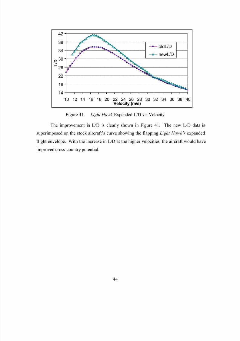
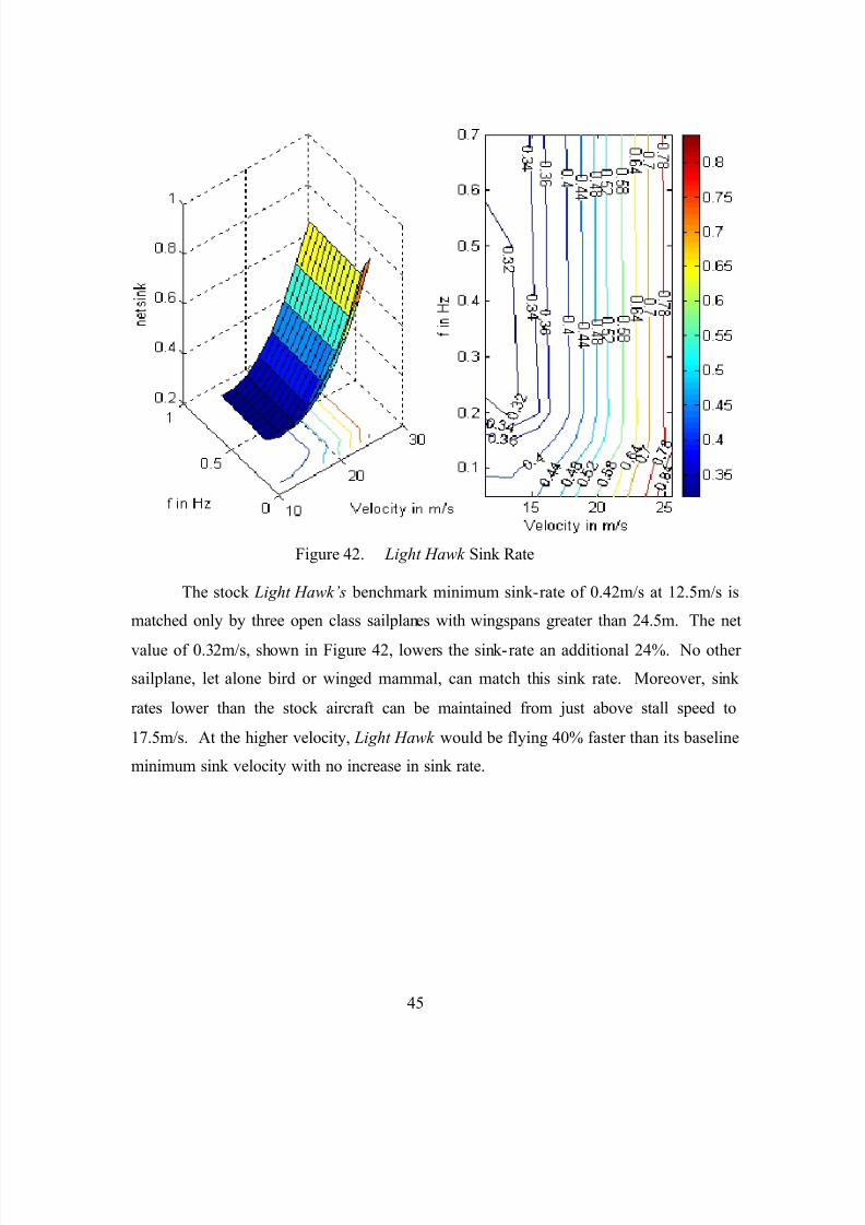
Figure 41. Light Hawk Expanded L/D vs. Velocity..........................................................44Figure 42. Light Hawk Sink Rate......................................................................................45
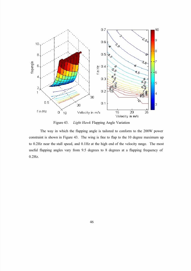
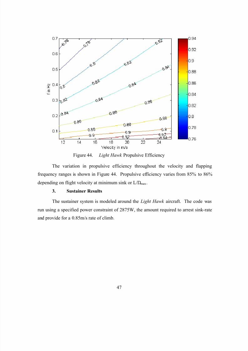
Figure 43. Light Hawk Flapping Angle Variation............................................................46Figure 44. Light Hawk Propulsive Efficiency...................................................................47
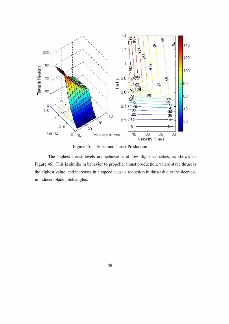
Figure 45. Sustainer Thrust Production ............................................................................48
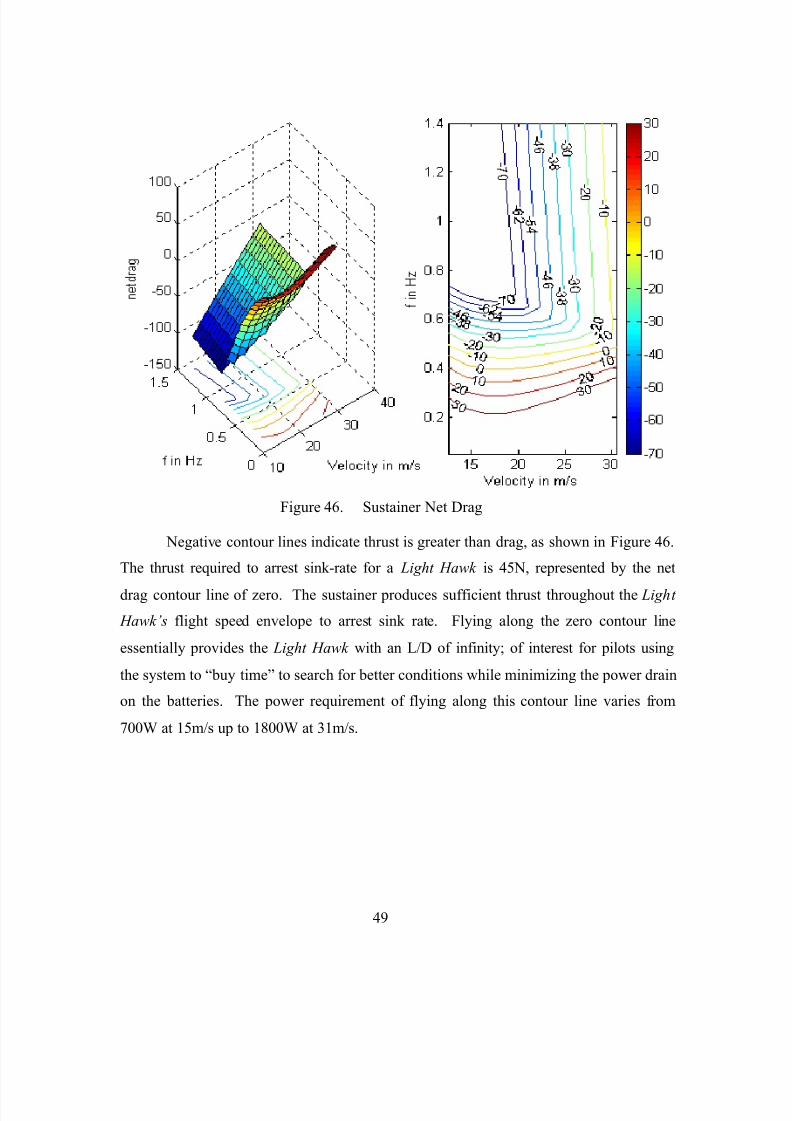
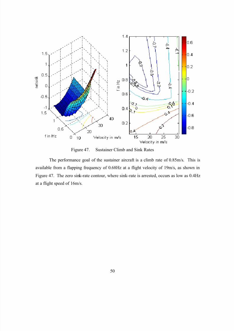
Figure 46. Sustainer Net Drag........................................................................................... 49Figure 47. Sustainer Climb and Sink Rates ......................................................................50
Figure 48. Sustainer Propulsive Efficiency.......................................................................51

7/18/2019 02Sep Randall
http://slidepdf.com/reader/full/02sep-randall 15/112
xiii
ACKNOWLEDGMENTS
I would like to thank Professors Kevin D. Jones and Max F. Platzer for their
guidance, countless instruction sessions, time, and patience in the completion of this
study. I wish to thank Steve Pollard for providing CMARC solutions necessary for the
validation of the numerical method employed in this study. I also wish to thank the
numerous sailplane manufacturers for providing information on their aircraft; in
particular, Greg Cole, of Windward Performance for data on the SparrowHawk ultralight
sailplane, as well as Danny Howell for data on the Light Hawk ultralight sailplane.
Last, but not least, I would like to thank my wife, Amy, for her tireless support.

7/18/2019 02Sep Randall
http://slidepdf.com/reader/full/02sep-randall 16/112
xiv
THIS PAGE INTENTIONALLY LEFT BLANK
7/18/2019 02Sep Randall
http://slidepdf.com/reader/full/02sep-randall 17/112
1
I. INTRODUCTION
A. OVERVIEW
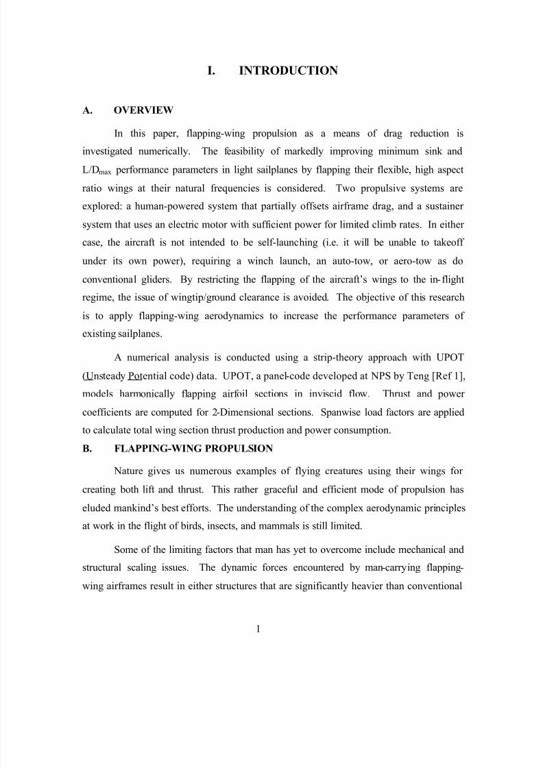
In this paper, flapping-wing propulsion as a means of drag reduction is
investigated numerically. The feasibility of markedly improving minimum sink and
L/Dmax performance parameters in light sailplanes by flapping their flexible, high aspect
ratio wings at their natural frequencies is considered. Two propulsive systems are
explored: a human-powered system that partially offsets airframe drag, and a sustainer
system that uses an electric motor with sufficient power for limited climb rates. In either
case, the aircraft is not intended to be self-launching (i.e. it will be unable to takeoff
under its own power), requiring a winch launch, an auto-tow, or aero-tow as do
conventional gliders. By restricting the flapping of the aircraft’s wings to the in- flight
regime, the issue of wingtip/ground clearance is avoided. The objective of this research
is to apply flapping-wing aerodynamics to increase the performance parameters of
existing sailplanes.
A numerical analysis is conducted using a strip-theory approach with UPOT
(Unsteady Potential code) data. UPOT, a panel-code developed at NPS by Teng [Ref 1],
models harmonically flapping airfoil sections in inviscid flow. Thrust and power
coefficients are computed for 2-Dimensional sections. Spanwise load factors are applied
to calculate total wing section thrust production and power consumption.
B. FLAPPING-WING PROPULSION
Nature gives us numerous examples of flying creatures using their wings for
creating both lift and thrust. This rather graceful and efficient mode of propulsion has
eluded mankind’s best efforts. The understanding of the complex aerodynamic principles
at work in the flight of birds, insects, and mammals is still limited.
Some of the limiting factors that man has yet to overcome include mechanical and
structural scaling issues. The dynamic forces encountered by man-carrying flapping-
wing airframes result in either structures that are significantly heavier than conventional
7/18/2019 02Sep Randall
http://slidepdf.com/reader/full/02sep-randall 18/112
2
airframes, or structures unable to withstand the dynamic forces of this method of
propulsion.
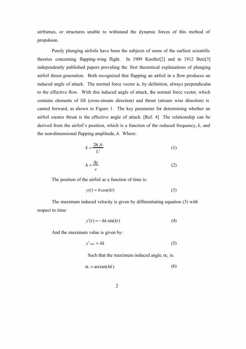
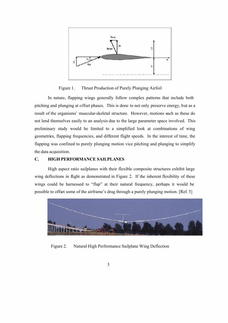
Purely plunging airfoils have been the subjects of some of the earliest scientific
theories concerning flapping-wing flight. In 1909 Knoller[2] and in 1912 Betz[3]independently published papers providing the first theoretical explanations of plunging
airfoil thrust generation. Both recognized that flapping an airfoil in a flow produces an
induced angle of attack. The normal force vector is, by definition, always perpendicular
to the effective flow. With this induced angle of attack, the normal force vector, which
contains elements of lift (cross-stream direction) and thrust (stream wise direction) is
canted forward, as shown in Figure 1. The key parameter for determining whether an
airfoil creates thrust is the effective angle of attack. [Ref. 4] The relationship can be
derived from the airfoil’s position, which is a function of the reduced frequency, k , and
the non-dimensional flapping amplitude, h. Where:
2 fck
U
π= (1)
yh
c
∆= (2)
The position of the airfoil as a function of time is:
( ) cos( ) y t h kt = (3)
The maximum induced velocity is given by differentiating equation (3) with
respect to time:
( ) sin( ) y t hk kt ′ = − (4)
And the maximum value is given by:
max y hk ′ = (5)
Such that the maximum induced angle, αi, is:
arctan( )i hk α = (6)
7/18/2019 02Sep Randall
http://slidepdf.com/reader/full/02sep-randall 19/112
3
Figure 1. Thrust Production of Purely Plunging Airfoil
In nature, flapping wings generally follow complex patterns that include both
pitching and plunging at offset phases. This is done to not only preserve energy, but as a
result of the organisms’ muscular-skeletal structure. However, motions such as these do
not lend themselves easily to an analysis due to the large parameter space involved. This
preliminary study would be limited to a simplified look at combinations of wing
geometries, flapping frequencies, and different flight speeds. In the interest of time, the
flapping was confined to purely plunging motion vice pitching and plunging to simplify
the data acquisition.
C. HIGH PERFORMANCE SAILPLANES
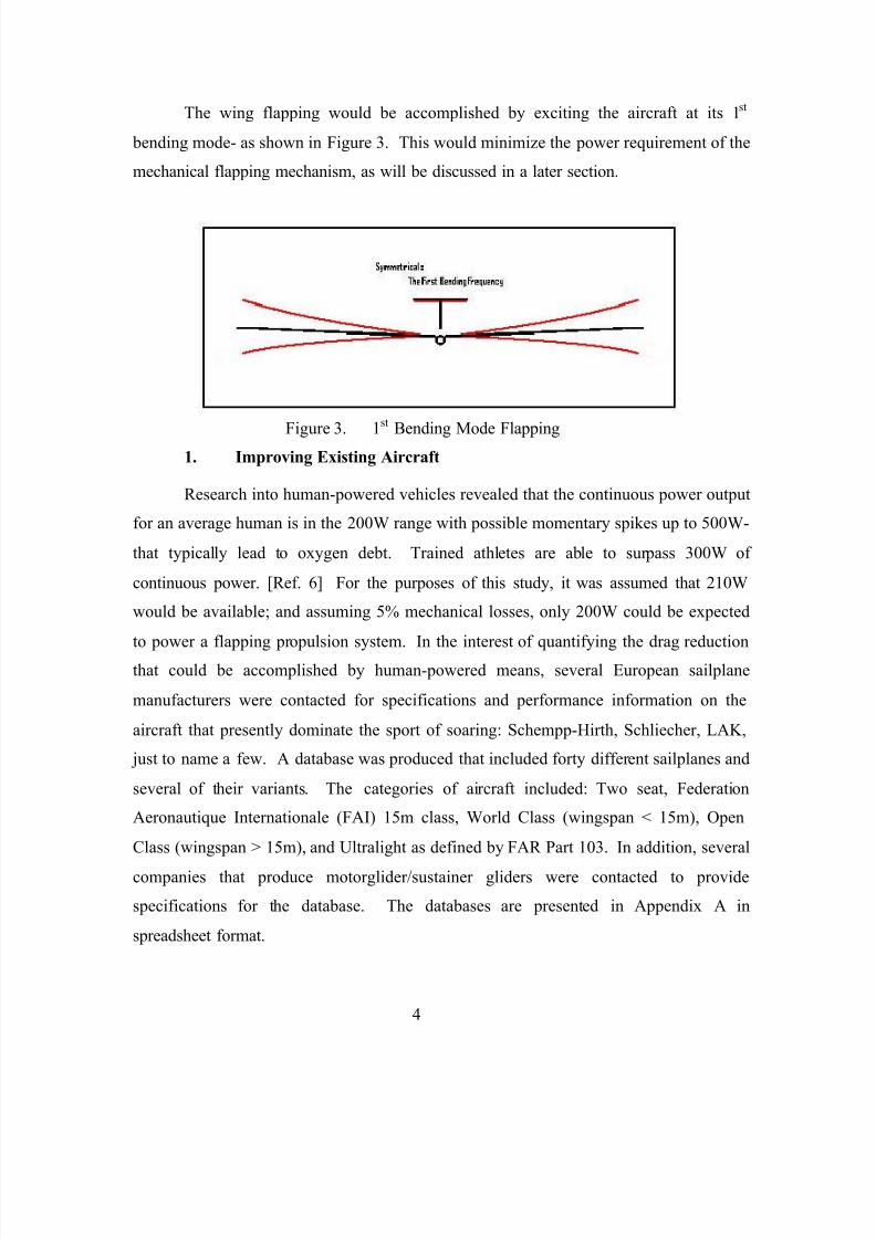
High aspect ratio sailplanes with their flexible composite structures exhibit largewing deflections in flight as demonstrated in Figure 2. If the inherent flexibility of these
wings could be harnessed to “flap” at their natural frequency, perhaps it would be
possible to offset some of the airframe’s drag through a purely plunging motion. [Ref. 5]
Figure 2. Natural High Performance Sailplane Wing Deflection
7/18/2019 02Sep Randall
http://slidepdf.com/reader/full/02sep-randall 20/112
4
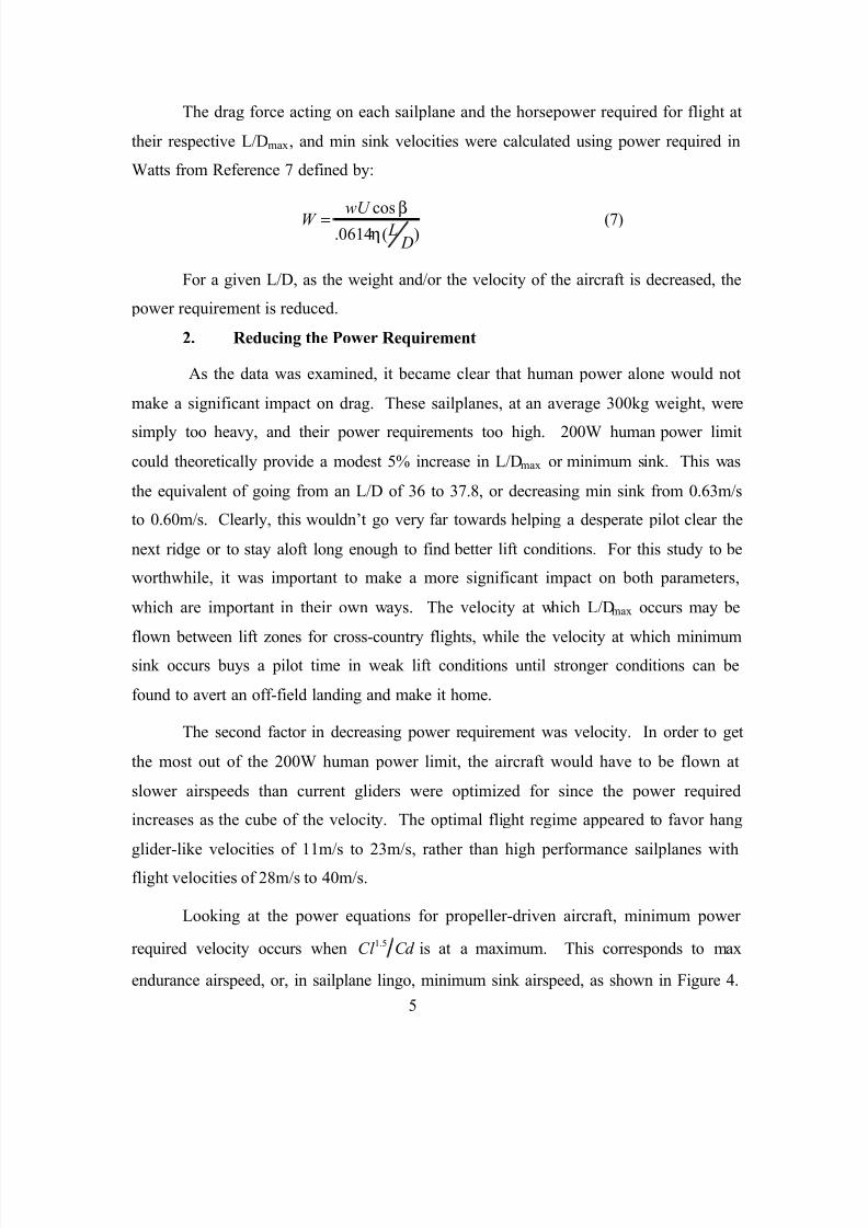
The wing flapping would be accomplished by exciting the aircraft at its 1st
bending mode- as shown in Figure 3. This would minimize the power requirement of the
mechanical flapping mechanism, as will be discussed in a later section.
Figure 3. 1
st
Bending Mode Flapping1. Improving Existing Aircraft
Research into human-powered vehicles revealed that the continuous power output
for an average human is in the 200W range with possible momentary spikes up to 500W-
that typically lead to oxygen debt. Trained athletes are able to surpass 300W of
continuous power. [Ref. 6] For the purposes of this study, it was assumed that 210W
would be available; and assuming 5% mechanical losses, only 200W could be expected
to power a flapping propulsion system. In the interest of quantifying the drag reduction
that could be accomplished by human-powered means, several European sailplane
manufacturers were contacted for specifications and performance information on the
aircraft that presently dominate the sport of soaring: Schempp-Hirth, Schliecher, LAK,
just to name a few. A database was produced that included forty different sailplanes and
several of their variants. The categories of aircraft included: Two seat, Federation
Aeronautique Internationale (FAI) 15m class, World Class (wingspan < 15m), Open
Class (wingspan > 15m), and Ultralight as defined by FAR Part 103. In addition, several
companies that produce motorglider/sustainer gliders were contacted to provide
specifications for the database. The databases are presented in Appendix A in
spreadsheet format.
7/18/2019 02Sep Randall
http://slidepdf.com/reader/full/02sep-randall 21/112
5
The drag force acting on each sailplane and the horsepower required for flight at
their respective L/Dmax, and min sink velocities were calculated using power required in
Watts from Reference 7 defined by:
cos.0614 ( )
wU W L
D
βη
= (7)
For a given L/D, as the weight and/or the velocity of the aircraft is decreased, the
power requirement is reduced.
2. Reducing the Power Requirement
As the data was examined, it became clear that human power alone would not
make a significant impact on drag. These sailplanes, at an average 300kg weight, were
simply too heavy, and their power requirements too high. 200W human power limit
could theoretically provide a modest 5% increase in L/Dmax or minimum sink. This was
the equivalent of going from an L/D of 36 to 37.8, or decreasing min sink from 0.63m/s
to 0.60m/s. Clearly, this wouldn’t go very far towards helping a desperate pilot clear the
next ridge or to stay aloft long enough to find better lift conditions. For this study to be
worthwhile, it was important to make a more significant impact on both parameters,
which are important in their own ways. The velocity at which L/Dmax occurs may be
flown between lift zones for cross-country flights, while the velocity at which minimumsink occurs buys a pilot time in weak lift conditions until stronger conditions can be
found to avert an off-field landing and make it home.
The second factor in decreasing power requirement was velocity. In order to get
the most out of the 200W human power limit, the aircraft would have to be flown at
slower airspeeds than current gliders were optimized for since the power required
increases as the cube of the velocity. The optimal flight regime appeared to favor hang
glider-like velocities of 11m/s to 23m/s, rather than high performance sailplanes with
flight velocities of 28m/s to 40m/s.
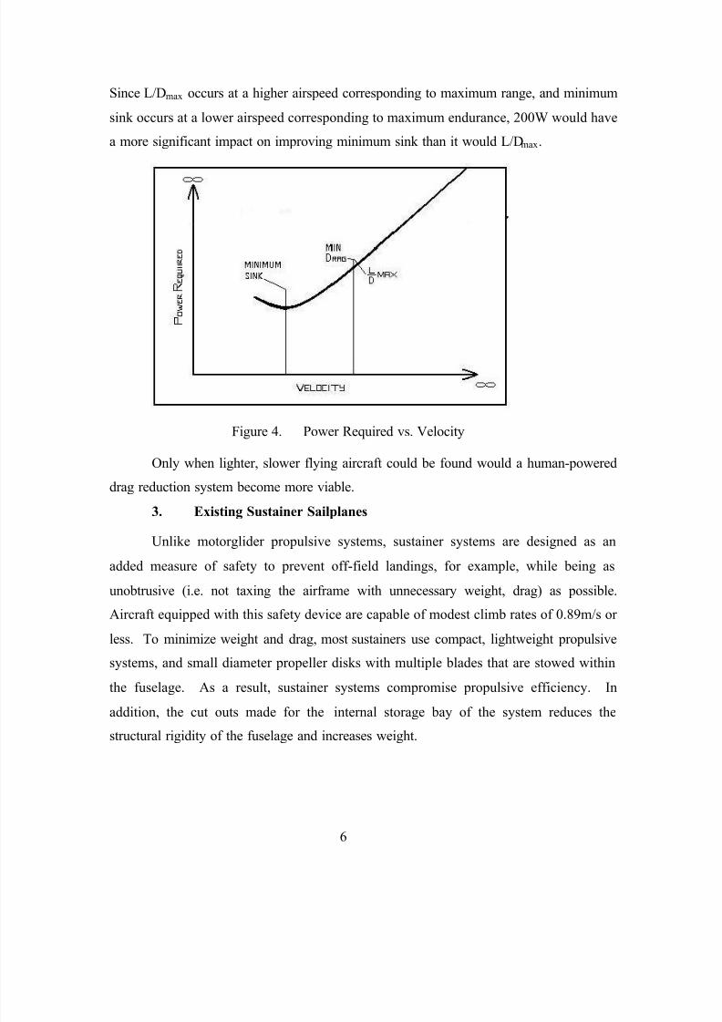
Looking at the power equations for propeller-driven aircraft, minimum power
required velocity occurs when 1.5Cl Cd is at a maximum. This corresponds to max
endurance airspeed, or, in sailplane lingo, minimum sink airspeed, as shown in Figure 4.
7/18/2019 02Sep Randall
http://slidepdf.com/reader/full/02sep-randall 22/112
6
Since L/Dmax occurs at a higher airspeed corresponding to maximum range, and minimum
sink occurs at a lower airspeed corresponding to maximum endurance, 200W would have
a more significant impact on improving minimum sink than it would L/Dmax.
Figure 4. Power Required vs. Velocity
Only when lighter, slower flying aircraft could be found would a human-powered
drag reduction system become more viable.
3. Existing Sustainer Sailplanes
Unlike motorglider propulsive systems, sustainer systems are designed as an
added measure of safety to prevent off-field landings, for example, while being as
unobtrusive (i.e. not taxing the airframe with unnecessary weight, drag) as possible.
Aircraft equipped with this safety device are capable of modest climb rates of 0.89m/s or
less. To minimize weight and drag, most sustainers use compact, lightweight propulsive
systems, and small diameter propeller disks with multiple blades that are stowed within
the fuselage. As a result, sustainer systems compromise propulsive efficiency. In
addition, the cut outs made for the internal storage bay of the system reduces thestructural rigidity of the fuselage and increases weight.
7/18/2019 02Sep Randall
http://slidepdf.com/reader/full/02sep-randall 23/112
7
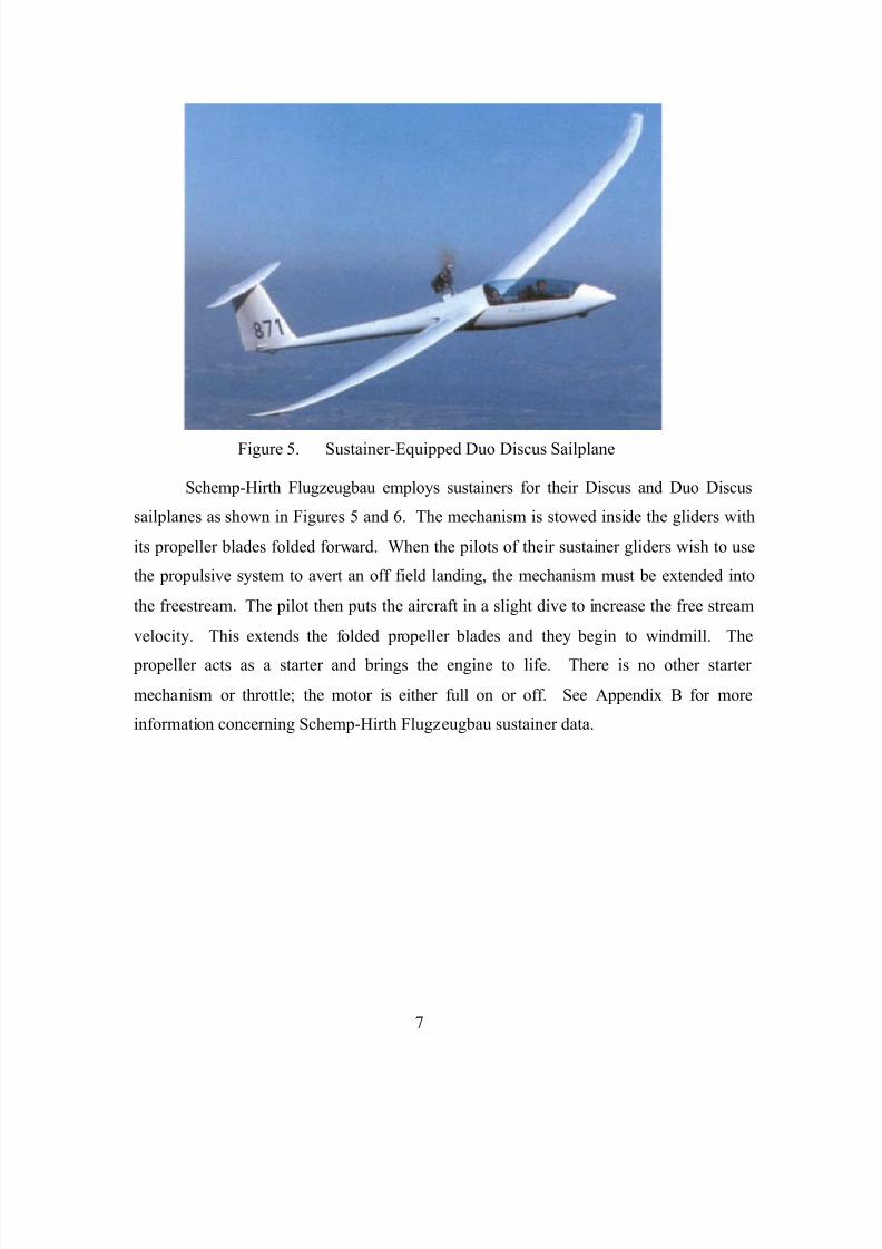
Figure 5. Sustainer-Equipped Duo Discus Sailplane
Schemp-Hirth Flugzeugbau employs sustainers for their Discus and Duo Discus
sailplanes as shown in Figures 5 and 6. The mechanism is stowed inside the gliders with
its propeller blades folded forward. When the pilots of their sustainer gliders wish to use
the propulsive system to avert an off field landing, the mechanism must be extended into
the freestream. The pilot then puts the aircraft in a slight dive to increase the free stream
velocity. This extends the folded propeller blades and they begin to windmill. The
propeller acts as a starter and brings the engine to life. There is no other starter
mechanism or throttle; the motor is either full on or off. See Appendix B for more
information concerning Schemp-Hirth Flugzeugbau sustainer data.
7/18/2019 02Sep Randall
http://slidepdf.com/reader/full/02sep-randall 24/112
8
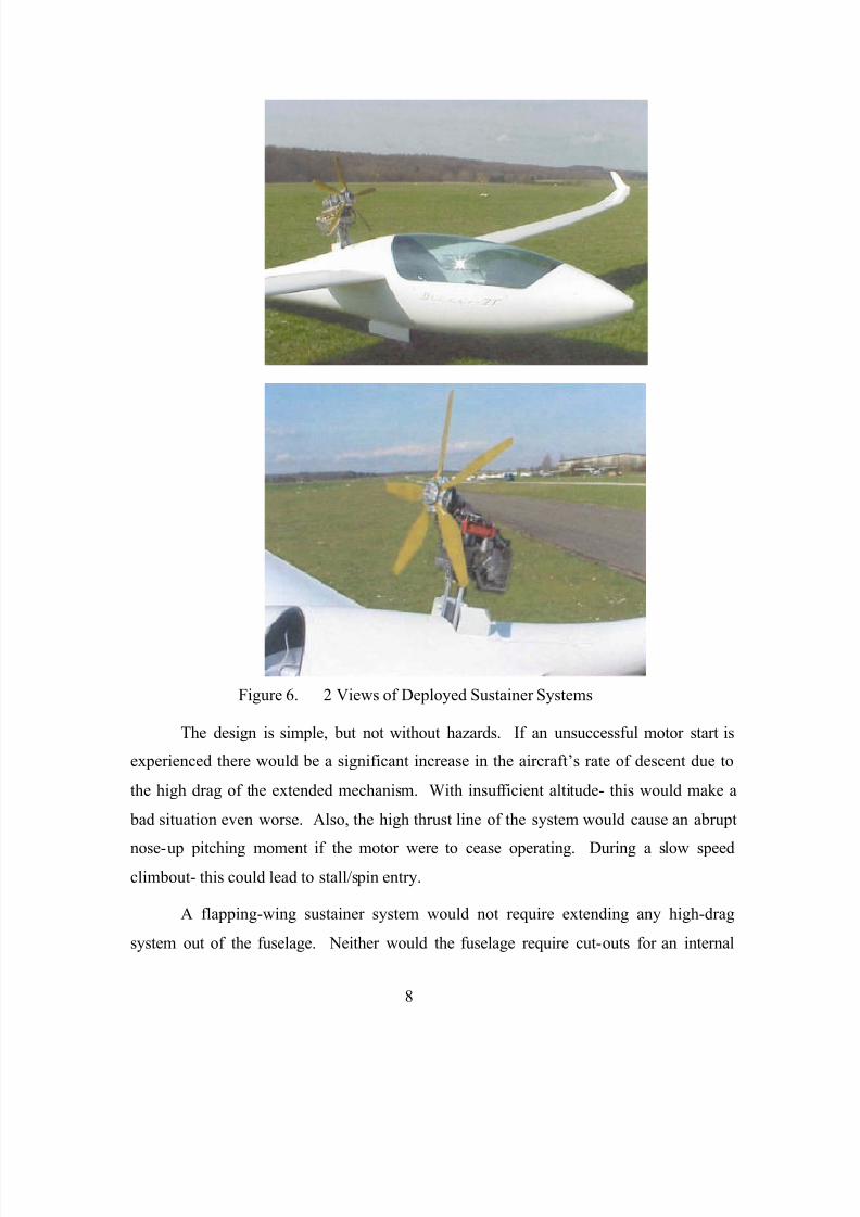
Figure 6. 2 Views of Deployed Sustainer Systems
The design is simple, but not without hazards. If an unsuccessful motor start is
experienced there would be a significant increase in the aircraft’s rate of descent due to
the high drag of the extended mechanism. With insufficient altitude- this would make a
bad situation even worse. Also, the high thrust line of the system would cause an abrupt
nose-up pitching moment if the motor were to cease operating. During a slow speedclimbout- this could lead to stall/spin entry.
A flapping-wing sustainer system would not require extending any high-drag
system out of the fuselage. Neither would the fuselage require cut-outs for an internal
7/18/2019 02Sep Randall
http://slidepdf.com/reader/full/02sep-randall 25/112
9
bay. Finally, this study will show that a sustainer system need not be a compromise in
propulsive efficiency.
4. Ultralight Sailplanes
Data from existing sailplanes began to show that human-powered drag reductionwould not be practical due to the limited effect 200W afforded to current relatively heavy
sailplanes. However, several sailplane manufacturers showcased new aircraft at the
Soaring Society of America’s Air Expo in Los Angeles in February of 2002. Most
notable were Windward Performance’s SparrowHawk , and Pure-Flight’s Light Hawk
aircraft. Both of these aircraft fall into the ultralight aircraft category as defined by FAR
Part 103. As per regulations, ultralight aircraft must weigh less than 70.3kg if
unpowered, and 115.2kg if powered. See Appendix B for more information concerning
FAR Part 103 regulations.
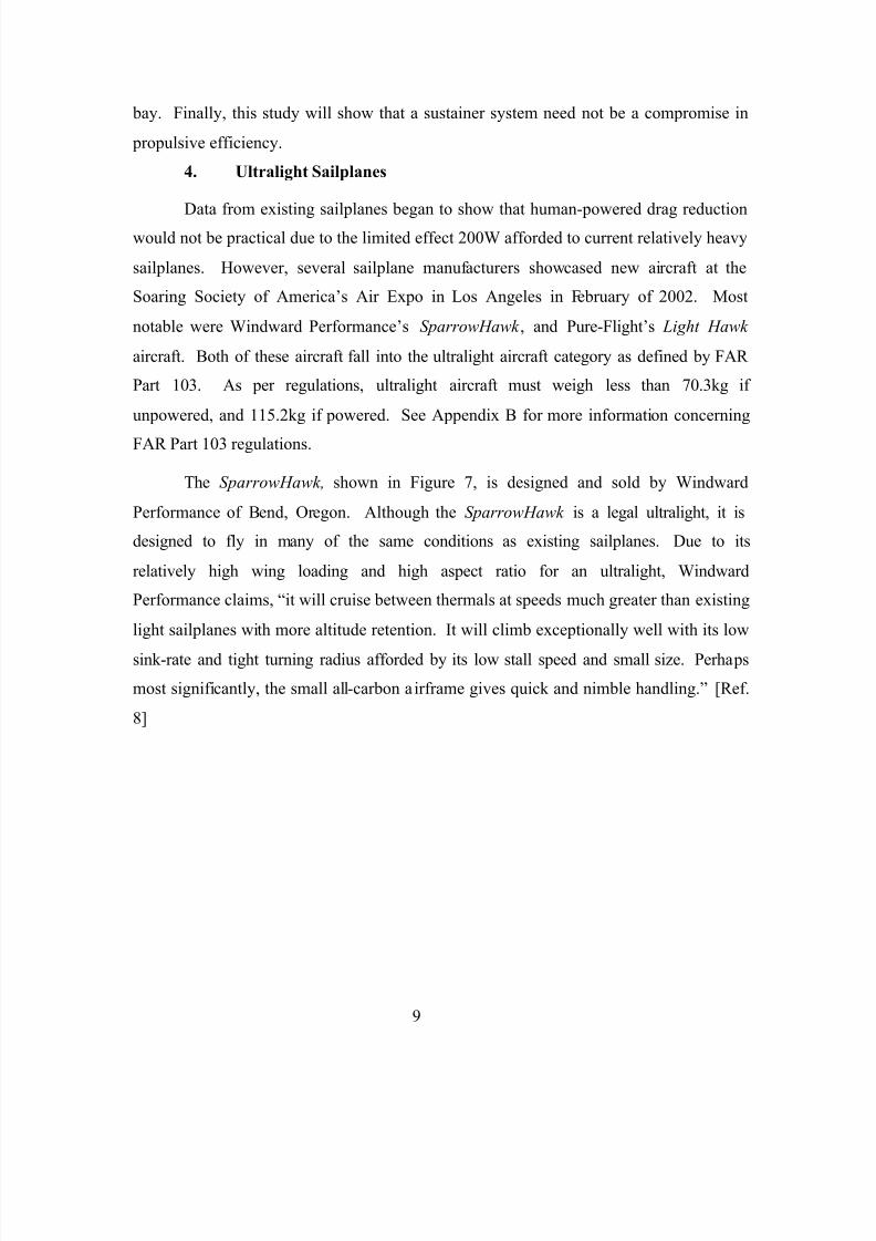
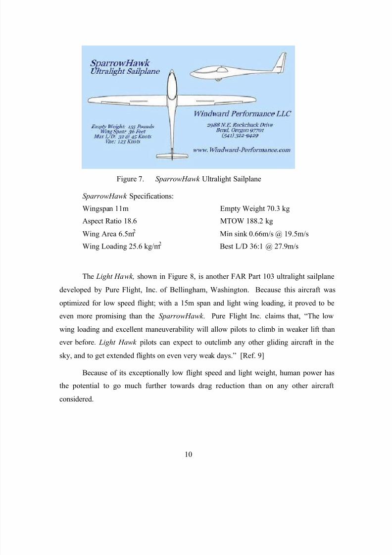
The SparrowHawk, shown in Figure 7, is designed and sold by Windward
Performance of Bend, Oregon. Although the SparrowHawk is a legal ultralight, it is
designed to fly in many of the same conditions as existing sailplanes. Due to its
relatively high wing loading and high aspect ratio for an ultralight, Windward
Performance claims, “it will cruise between thermals at speeds much greater than existing
light sailplanes with more altitude retention. It will climb exceptionally well with its low
sink-rate and tight turning radius afforded by its low stall speed and small size. Perhaps
most significantly, the small all-carbon airframe gives quick and nimble handling.” [Ref.
8]
7/18/2019 02Sep Randall
http://slidepdf.com/reader/full/02sep-randall 26/112
10
Figure 7. SparrowHawk Ultralight Sailplane
SparrowHawk Specifications:
Wingspan 11m Empty Weight 70.3 kg
Aspect Ratio 18.6 MTOW 188.2 kg
Wing Area 6.5m2 Min sink 0.66m/s @ 19.5m/s
Wing Loading 25.6 kg/m2 Best L/D 36:1 @ 27.9m/s
The Light Hawk, shown in Figure 8, is another FAR Part 103 ultralight sailplane
developed by Pure Flight, Inc. of Bellingham, Washington. Because this aircraft wasoptimized for low speed flight; with a 15m span and light wing loading, it proved to be
even more promising than the SparrowHawk . Pure Flight Inc. claims that, “The low
wing loading and excellent maneuverability will allow pilots to climb in weaker lift than
ever before. Light Hawk pilots can expect to outclimb any other gliding aircraft in the
sky, and to get extended flights on even very weak days.” [Ref. 9]
Because of its exceptionally low flight speed and light weight, human power has
the potential to go much further towards drag reduction than on any other aircraftconsidered.
7/18/2019 02Sep Randall
http://slidepdf.com/reader/full/02sep-randall 27/112
11
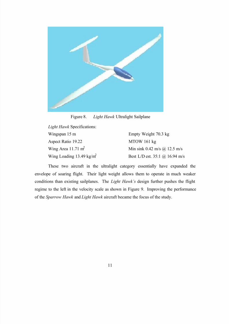
Figure 8. Light Hawk Ultralight Sailplane
Light Hawk Specifications:
Wingspan 15 m Empty Weight 70.3 kg
Aspect Ratio 19.22 MTOW 161 kg
Wing Area 11.71 m2 Min sink 0.42 m/s @ 12.5 m/s
Wing Loading 13.49 kg/m2 Best L/D est. 35:1 @ 16.94 m/s
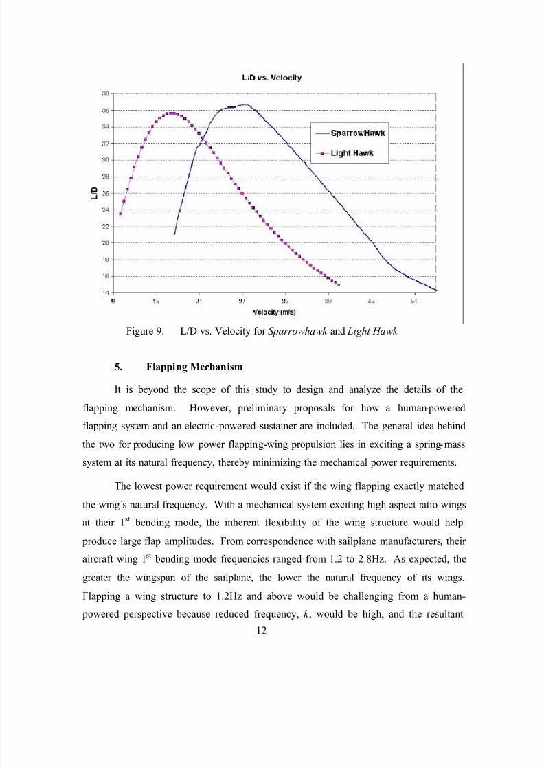
These two aircraft in the ultralight category essentially have expanded the
envelope of soaring flight. Their light weight allows them to operate in much weaker
conditions than existing sailplanes. The Light Hawk’s design further pushes the flight
regime to the left in the velocity scale as shown in Figure 9. Improving the performance
of the Sparrow Hawk and Light Hawk aircraft became the focus of the study.
7/18/2019 02Sep Randall
http://slidepdf.com/reader/full/02sep-randall 28/112
12
Figure 9. L/D vs. Velocity for Sparrowhawk and Light Hawk
5. Flapping Mechanism
It is beyond the scope of this study to design and analyze the details of the
flapping mechanism. However, preliminary proposals for how a human-powered
flapping system and an electric-powered sustainer are included. The general idea behind
the two for producing low power flapping-wing propulsion lies in exciting a spring-mass
system at its natural frequency, thereby minimizing the mechanical power requirements.
The lowest power requirement would exist if the wing flapping exactly matched
the wing’s natural frequency. With a mechanical system exciting high aspect ratio wings
at their 1st bending mode, the inherent flexibility of the wing structure would help
produce large flap amplitudes. From correspondence with sailplane manufacturers, their
aircraft wing 1st bending mode frequencies ranged from 1.2 to 2.8Hz. As expected, the
greater the wingspan of the sailplane, the lower the natural frequency of its wings.
Flapping a wing structure to 1.2Hz and above would be challenging from a human-
powered perspective because reduced frequency, k , would be high, and the resultant
7/18/2019 02Sep Randall
http://slidepdf.com/reader/full/02sep-randall 29/112
13
propulsive efficiency, η, would be low. However, there are ways to lower the natural
frequency of a wing structure: decreasing its stiffness, or adding mass, for example.
Decreasing the stiffness of the structure was deemed unacceptable as it would require
extensive modifications to existing wings, and it would decrease the dive speed of the
aircraft. Adding weight to an aircraft is not desirable either. However, the penalty is
minimized by adding weight at the wing tips. To “tune” the 1st bending mode to a more
achievable range, it was hoped that this method would be the least intrusive from a
performance perspective.
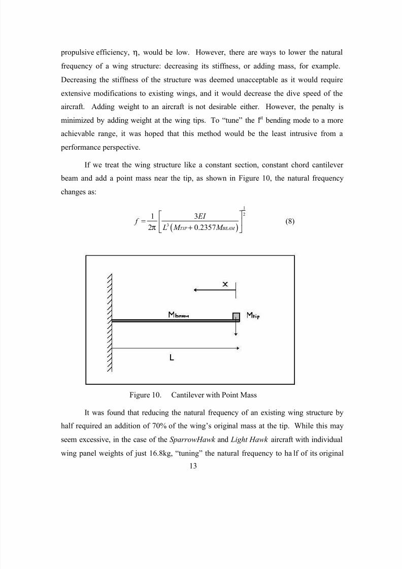
If we treat the wing structure like a constant section, constant chord cantilever
beam and add a point mass near the tip, as shown in Figure 10, the natural frequency
changes as:
( )
1
2
3
1 3
2 0.2357TIP BEAM
EI f
L M M π
=
+ (8)
Figure 10. Cantilever with Point Mass
It was found that reducing the natural frequency of an existing wing structure by
half required an addition of 70% of the wing’s original mass at the tip. While this may
seem excessive, in the case of the SparrowHawk and Light Hawk aircraft with individual
wing panel weights of just 16.8kg, “tuning” the natural frequency to ha lf of its original
7/18/2019 02Sep Randall
http://slidepdf.com/reader/full/02sep-randall 30/112
14
value could be achieved by adding 11.8kg of water ballast at the wing tips, the equivalent
of 4.4gallons for each wing. Because wing sections are tapered, and have more of their
mass near the root, the true ballast requirement would probably be lower. Since many of
today’s competition gliders incorporate water ballast tanks much larger than this inside
their wings- adding tanks near the wing tips would not be an unreasonable modification.
However, to lower the natural frequency even more, the required additional mass would
become excessive. In addition, with wing tip ballast in place, consideration must be
given to a reduction in flight speeds to avoid the possibility of flutter. Therefore, in order
to not limit either aircraft’s performance, the addition of mass would be used as a
secondary means to fine-tune the aircraft’s natural frequency to the range that offers the
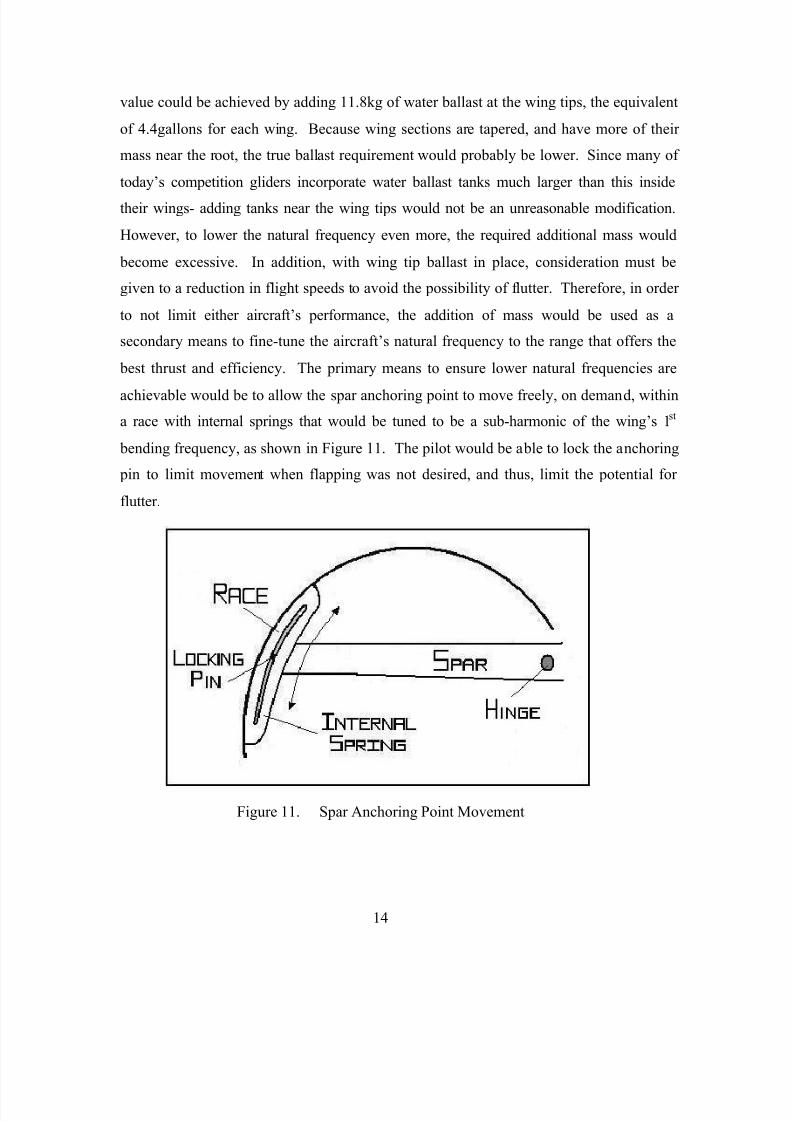
best thrust and efficiency. The primary means to ensure lower natural frequencies are
achievable would be to allow the spar anchoring point to move freely, on demand, within
a race with internal springs that would be tuned to be a sub-harmonic of the wing’s 1st
bending frequency, as shown in Figure 11. The pilot would be able to lock the anchoring
pin to limit movement when flapping was not desired, and thus, limit the potential for
flutter.
Figure 11. Spar Anchoring Point Movement
7/18/2019 02Sep Randall
http://slidepdf.com/reader/full/02sep-randall 31/112
15
a. Human-Powered System
Employing a bicycle-type pedal system with a front sprocket, rear
sprocket, and a chain to transfer power to the movement of the wings, the mechanical
losses could be expected to be low. A simple bicycle chain is one of the mostmechanically efficient drive systems available; with efficiencies up to 98.6%. This
means that less than 2 percent of the power used to turn a bike train is lost to friction-
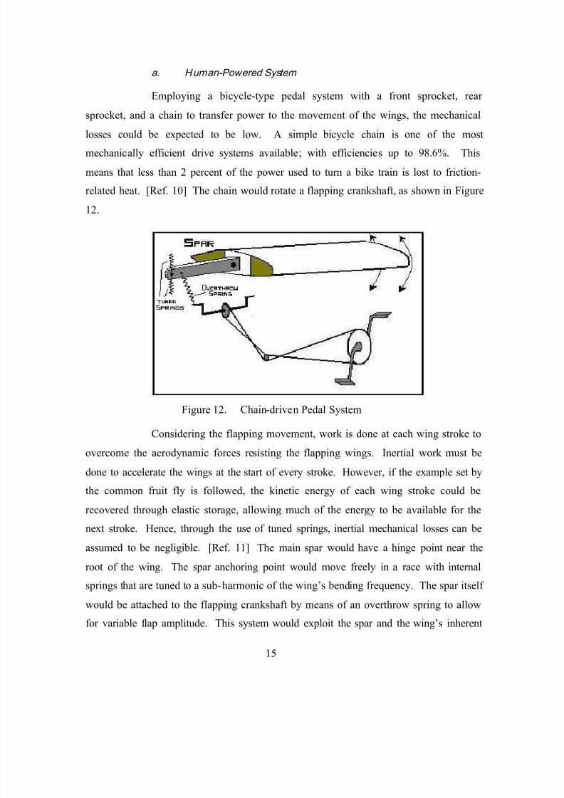
related heat. [Ref. 10] The chain would rotate a flapping crankshaft, as shown in Figure
12.
Figure 12. Chain-driven Pedal System
Considering the flapping movement, work is done at each wing stroke to
overcome the aerodynamic forces resisting the flapping wings. Inertial work must be
done to accelerate the wings at the start of every stroke. However, if the example set by
the common fruit fly is followed, the kinetic energy of each wing stroke could be
recovered through elastic storage, allowing much of the energy to be available for the
next stroke. Hence, through the use of tuned springs, inertial mechanical losses can be
assumed to be negligible. [Ref. 11] The main spar would have a hinge point near the
root of the wing. The spar anchoring point would move freely in a race with internal
springs that are tuned to a sub-harmonic of the wing’s bending frequency. The spar itself
would be attached to the flapping crankshaft by means of an overthrow spring to allow
for variable flap amplitude. This system would exploit the spar and the wing’s inherent
7/18/2019 02Sep Randall
http://slidepdf.com/reader/full/02sep-randall 32/112
16
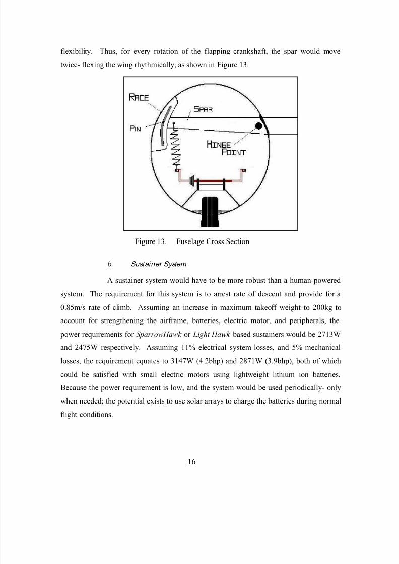
flexibility. Thus, for every rotation of the flapping crankshaft, the spar would move
twice- flexing the wing rhythmically, as shown in Figure 13.
Figure 13. Fuselage Cross Section
b. Sustainer System
A sustainer system would have to be more robust than a human-powered
system. The requirement for this system is to arrest rate of descent and provide for a0.85m/s rate of climb. Assuming an increase in maximum takeoff weight to 200kg to
account for strengthening the airframe, batteries, electric motor, and peripherals, the
power requirements for SparrowHawk or Light Hawk based sustainers would be 2713W
and 2475W respectively. Assuming 11% electrical system losses, and 5% mechanical
losses, the requirement equates to 3147W (4.2bhp) and 2871W (3.9bhp), both of which
could be satisfied with small electric motors using lightweight lithium ion batteries.
Because the power requirement is low, and the system would be used periodically- only
when needed; the potential exists to use solar arrays to charge the batteries during normal
flight conditions.
7/18/2019 02Sep Randall
http://slidepdf.com/reader/full/02sep-randall 33/112
17
II. NUMERICAL ANALYSIS
A. STRIP-THEORY APPROACH
While 3-Dimensional tools may provide results with a higher level of detail, the
2-Dimensional strip-theory approach employed in this study provides an inexpensive
means to study a large parameter space. This is especially useful in studying flapping-
wing propulsion with its virtually infinite number of parameters. Once trends are made
visible through the strip-theory approach, more accurate methods can be used to provide
a closer look.
Critical to the method was the ability to treat drag and thrust independently. This
meant that as long as boundary layer separation was minimal, the profile drag of theaircraft encountered during normal flight (steady case) would not change in flapping-
wing flight (unsteady case). Then, the thrust produced through flapping would be
subtracted from the existing drag. From Reference 12: “Effectively, Ct only accounts for
the forces due to unsteady pressure distribution around the wing, since skin friction is
nearly constant in time and thus equal in steady and unsteady case.”
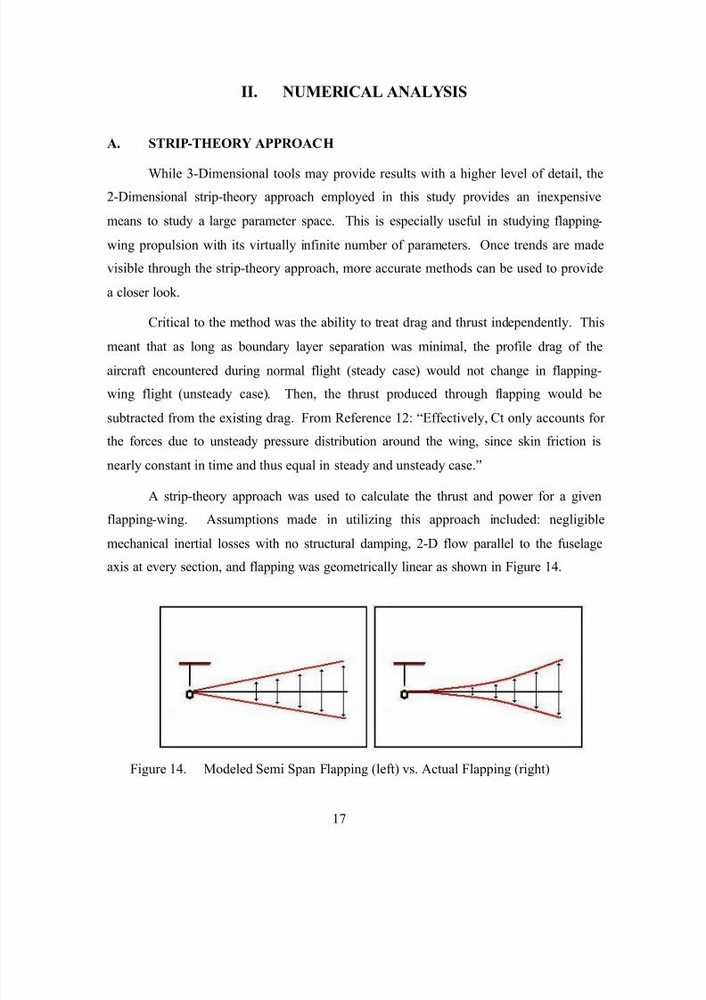
A strip-theory approach was used to calculate the thrust and power for a given
flapping-wing. Assumptions made in utilizing this approach included: negligiblemechanical inertial losses with no structural damping, 2-D flow parallel to the fuselage
axis at every section, and flapping was geometrically linear as shown in Figure 14.
Figure 14. Modeled Semi Span Flapping (left) vs. Actual Flapping (right)
7/18/2019 02Sep Randall
http://slidepdf.com/reader/full/02sep-randall 34/112
18
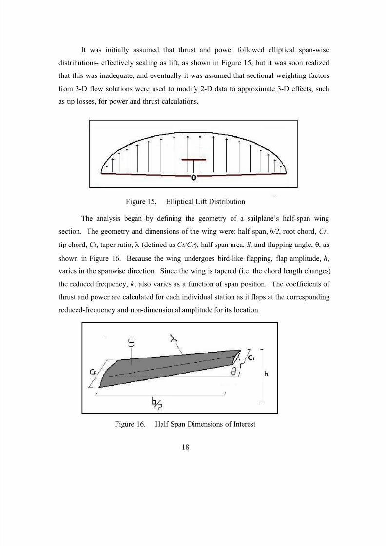
It was initially assumed that thrust and power followed elliptical span-wise
distributions- effectively scaling as lift, as shown in Figure 15, but it was soon realized
that this was inadequate, and eventually it was assumed that sectional weighting factors
from 3-D flow solutions were used to modify 2-D data to approximate 3-D effects, such
as tip losses, for power and thrust calculations.
Figure 15. Elliptical Lift Distribution
The analysis began by defining the geometry of a sailplane’s half-span wing
section. The geometry and dimensions of the wing were: half span, b/2, root chord, Cr ,
tip chord, Ct , taper ratio, λ (defined as Ct/Cr ), half span area, S , and flapping angle, θ, as
shown in Figure 16. Because the wing undergoes bird-like flapping, flap amplitude, h,
varies in the spanwise direction. Since the wing is tapered (i.e. the chord length changes)
the reduced frequency, k , also varies as a function of span position. The coefficients ofthrust and power are calculated for each individual station as it flaps at the corresponding
reduced-frequency and non-dimensional amplitude for its location.
Figure 16. Half Span Dimensions of Interest
7/18/2019 02Sep Randall
http://slidepdf.com/reader/full/02sep-randall 35/112
19
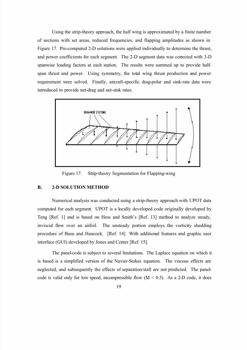
Using the strip-theory approach, the half wing is approximated by a finite number
of sections with set areas, reduced frequencies, and flapping amplitudes as shown in
Figure 17. Pre-computed 2-D solutions were applied individually to determine the thrust,
and power coefficients for each segment. The 2-D segment data was corrected with 3-D
spanwise loading factors at each station. The results were summed up to provide half-
span thrust and power. Using symmetry, the total wing thrust production and power
requirement were solved. Finally, aircraft-specific drag-polar and sink-rate data were
introduced to provide net-drag and net-sink rates.
Figure 17. Strip-theory Segmentation for Flapping-wing
B. 2-D SOLUTION METHOD
Numerical analysis was conducted using a strip-theory approach with UPOT data
computed for each segment. UPOT is a locally developed code originally developed by
Teng [Ref. 1] and is based on Hess and Smith’s [Ref. 13] method to analyze steady,
inviscid flow over an airfoil. The unsteady portion employs the vorticity shedding
procedure of Basu and Hancock. [Ref. 14] With additional features and graphic user
interface (GUI) developed by Jones and Center [Ref. 15].
The panel-code is subject to several limitations. The Laplace equation on which it
is based is a simplified version of the Navier-Stokes equation. The viscous effects are
neglected, and subsequently the effects of separation/stall are not predicted. The panel-
code is valid only for low speed, incompressible flow (M < 0.3). As a 2-D code, it does
7/18/2019 02Sep Randall
http://slidepdf.com/reader/full/02sep-randall 36/112
20
not analyze 3-D effects such as wing-tip vortices, however, it does predict unsteady
streamwise pressure contributions with results that agree well with theory, extensive
experimental work, and other numerical methods. [Ref. 16]
Maximum plunge speed occurs as the product of h and k. Recall from equation 6:
arctan( ) ihk α= (6)
When the product of h and k approaches 0.8, the airfoil experiences high-induced
angles of attack. Because airfoil stall is a progressive, not instantaneous development, a
plunging airfoil typically experiences the onset of dynamic stall at much higher values of
angle of attack. The peak value occurs when the airfoil passes through the midpoint of its
flapping sequence; where its vertical velocity is highest. As will be shown in a later
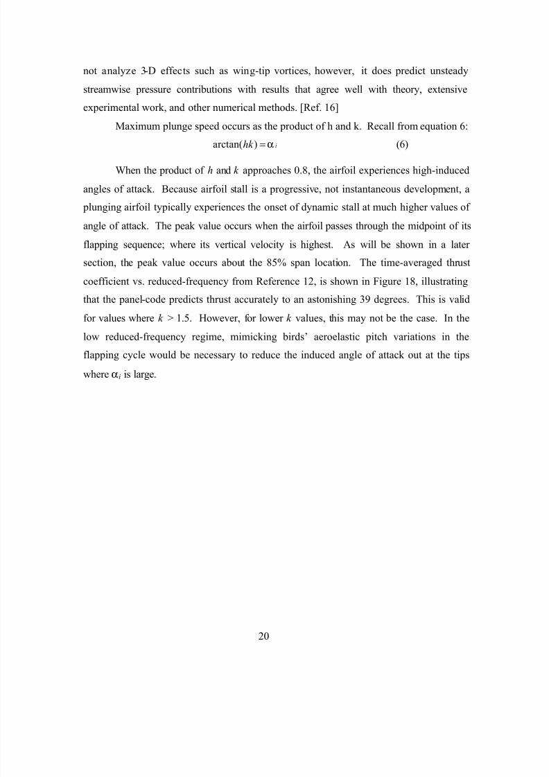
section, the peak value occurs about the 85% span location. The time-averaged thrust
coefficient vs. reduced-frequency from Reference 12, is shown in Figure 18, illustrating
that the panel-code predicts thrust accurately to an astonishing 39 degrees. This is valid
for values where k > 1.5. However, for lower k values, this may not be the case. In the
low reduced-frequency regime, mimicking birds’ aeroelastic pitch variations in the
flapping cycle would be necessary to reduce the induced angle of attack out at the tips
where αi is large.
7/18/2019 02Sep Randall
http://slidepdf.com/reader/full/02sep-randall 37/112
21
Figure 18. Time Averaged Thrust Coefficient vs. Reduced Frequency
Further details concerning the panel-code, UPOT, its validation, and its
limitations are available in references 1, 16, 18, 19.
Modern sailplane wings possess numerous variables at different span locations,
such as: optimized laminar and turbulent airfoils, transition areas for these different
airfoil sections, and complex multiple wing tapering; it was necessary to determine how
sensitive flapping-wing thrust production was to airfoil shape and angle of attack. If
these factors proved not to be critical, then a simplified 2-D panel method using a single
airfoil section would sufficiently approximate the flow around different sailplane wing
sections. Basically, the simple strip-theory approach will only work if thrust production
is independent of angle of attack and airfoil shape.
In Reference 12 it was shown that thrust production was independent to changes
in mean angle of attack. In Reference 18, the effect of airfoil thickness and camber on
thrust and power production for purely plunging airfoils was also shown to be negligible.
7/18/2019 02Sep Randall
http://slidepdf.com/reader/full/02sep-randall 38/112
22
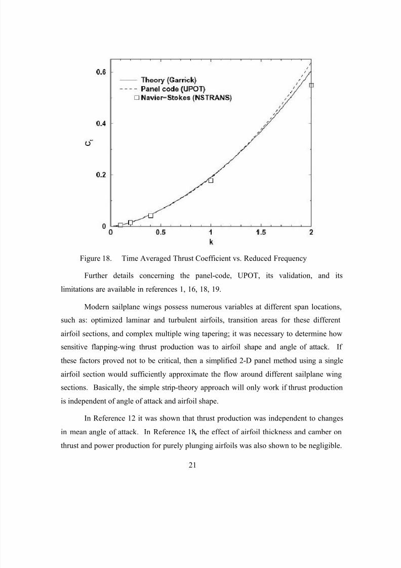
UPOT was used to verify data from these references. Several NACA airfoils of
increasing thickness were put through purely plunging motion in the UPOT code. The
range of flapping amplitude, h, was 0.25 to 2.0, while the range of reduced frequency, k ,
was 0.055 to 0.443.
0.4485
0.4487
0.4489
0.4491
0.4493
0.4495
0.4497
0.4499
0.4501
0.4503
0.4505
0.4507
0.4509
0.4511
0.4513
0.4515
0.4517
0.4519
7 8 9 10 11 12 13 14 15
Airfoil Percent Thickness
T h r u s t C o e f f i c i e n t
Figure 19. Airfoil Thickness vs. Thrust Coefficient
It was found that the effect of thickness on a purely plunging airfoil’s thrust
production is negligible. The plot in Figure 19 is misleading as it appears to show a
decrease in thrust as thickness increases. However, the vertical scale represents a very
small percentage change in thrust coefficient; well below the numerical accuracy of the
method.
Determining if thrust was sensitive to changes in airfoil camber was accomplished
by putting several NACA airfoils of increasing camber through purely plunging motion
in UPOT.
7/18/2019 02Sep Randall
http://slidepdf.com/reader/full/02sep-randall 39/112
23
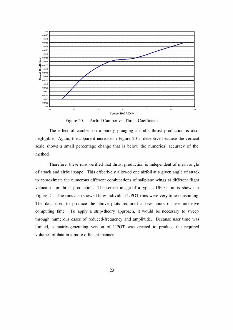
Figure 20. Airfoil Camber vs. Thrust Coefficient
The effect of camber on a purely plunging airfoil’s thrust production is also
negligible. Again, the apparent increase in Figure 20 is deceptive because the vertical
scale shows a small percentage change that is below the numerical accuracy of the
method.
Therefore, these runs verified that thrust production is independent of mean angle
of attack and airfoil shape. This effectively allowed one airfoil at a given angle of attackto approximate the numerous different combinations of sailplane wings at different flight
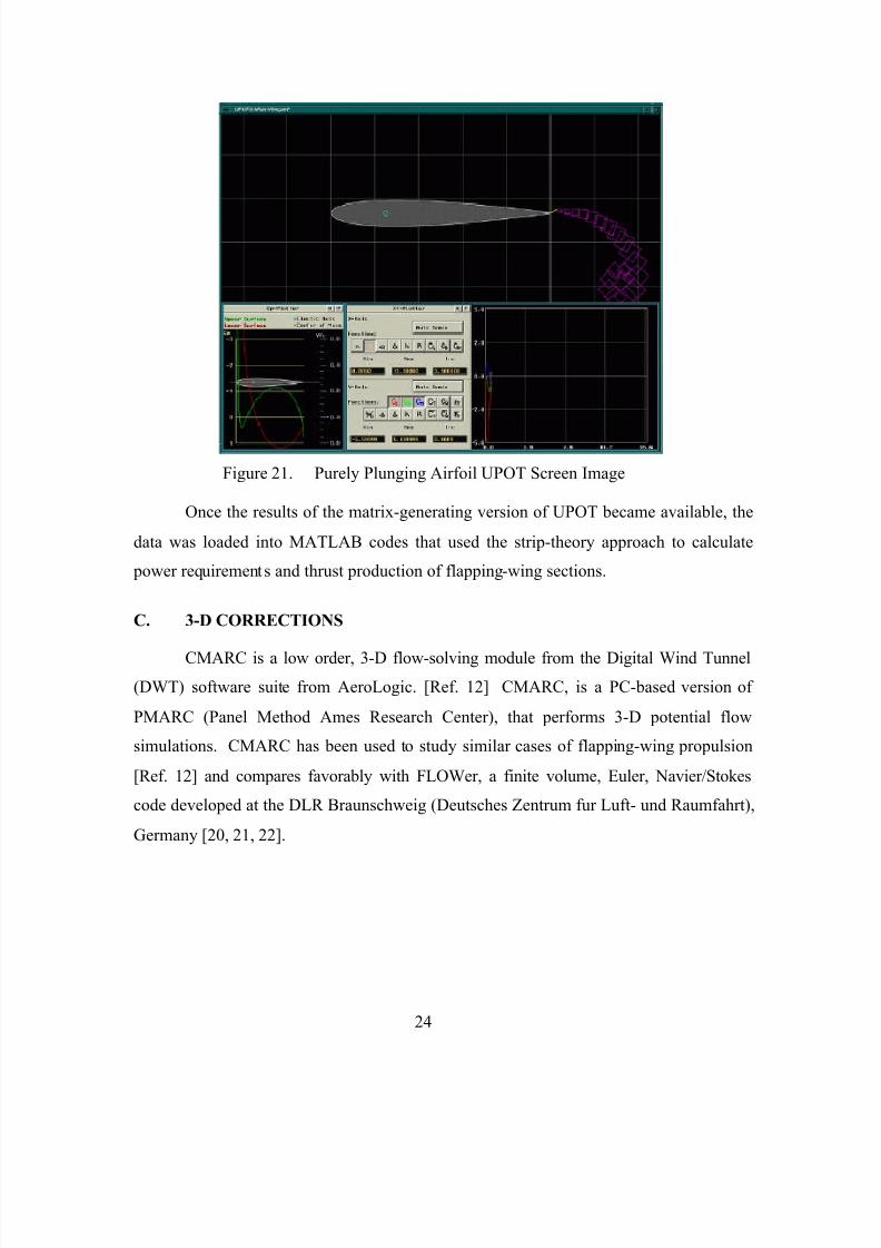
velocities for thrust production. The screen image of a typical UPOT run is shown in
Figure 21. The runs also showed how individual UPOT runs were very time-consuming.
The data used to produce the above plots required a few hours of user-intensive
computing time. To apply a strip-theory approach, it would be necessary to sweep
through numerous cases of reduced-frequency and amplitude. Because user time was
limited, a matrix-generating version of UPOT was created to produce the required
volumes of data in a more efficient manner.
0.44
0.4405
0.441
0.4415
0.442
0.4425
0.443
0.4435
0.444
0.4445
0.445
0.4455
0.446
0.4465
0.447
0.4475
0.448
0.4485
0.449
0.4495
0.45
13 15 17 19 21 23 25
Camber NACA XX14
T h r u s t C o e f f i c i e n
7/18/2019 02Sep Randall
http://slidepdf.com/reader/full/02sep-randall 40/112
24
Figure 21. Purely Plunging Airfoil UPOT Screen Image
Once the results of the matrix-generating version of UPOT became available, the
data was loaded into MATLAB codes that used the strip-theory approach to calculate
power requirements and thrust production of flapping-wing sections.
C. 3-D CORRECTIONS
CMARC is a low order, 3-D flow-solving module from the Digital Wind Tunnel
(DWT) software suite from AeroLogic. [Ref. 12] CMARC, is a PC-based version of
PMARC (Panel Method Ames Research Center), that performs 3-D potential flow
simulations. CMARC has been used to study similar cases of flapping-wing propulsion
[Ref. 12] and compares favorably with FLOWer, a finite volume, Euler, Navier/Stokes
code developed at the DLR Braunschweig (Deutsches Zentrum fur Luft- und Raumfahrt),
Germany [20, 21, 22].
7/18/2019 02Sep Randall
http://slidepdf.com/reader/full/02sep-randall 41/112
25
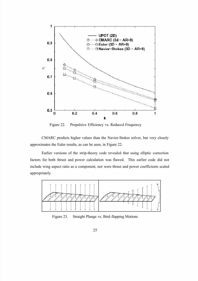
Figure 22. Propulsive Efficiency vs. Reduced Frequency
CMARC predicts higher values than the Navier-Stokes solver, but very closely
approximates the Euler results, as can be seen, in Figure 22.
Earlier versions of the strip-theory code revealed that using elliptic correction
factors for both thrust and power calculation was flawed. This earlier code did not
include wing aspect ratio as a component, nor were thrust and power coefficients scaled
appropriately.
Figure 23. Straight Plunge vs. Bird-flapping Motions
7/18/2019 02Sep Randall
http://slidepdf.com/reader/full/02sep-randall 42/112
26
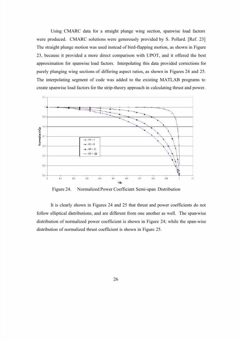
Using CMARC data for a straight plunge wing section, spanwise load factors
were produced. CMARC solutions were generously provided by S. Pollard. [Ref. 23]
The straight plunge motion was used instead of bird-flapping motion, as shown in Figure
23, because it provided a more direct comparison with UPOT, and it offered the best
approximation for spanwise load factors. Interpolating this data provided corrections for
purely plunging wing sections of differing aspect ratios, as shown in Figures 24 and 25.
The interpolating segment of code was added to the existing MATLAB programs to
create spanwise load factors for the strip-theory approach in calculating thrust and power.
Figure 24. Normalized Power Coefficient Semi-span Distribution
It is clearly shown in Figures 24 and 25 that thrust and power coefficients do not
follow elliptical distributions, and are different from one another as well. The span-wise
distribution of normalized power coefficient is shown in Figure 24; while the span-wise
distribution of normalized thrust coefficient is shown in Figure 25.
7/18/2019 02Sep Randall
http://slidepdf.com/reader/full/02sep-randall 43/112
27
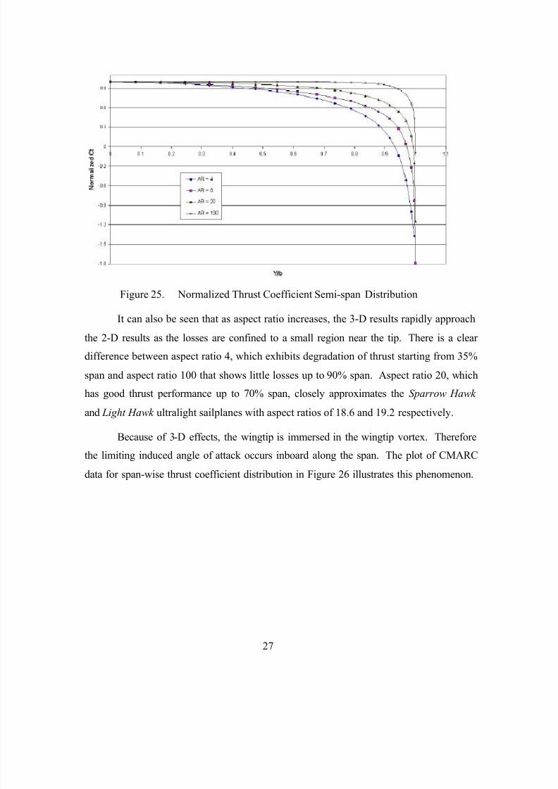
Figure 25. Normalized Thrust Coefficient Semi-span Distribution
It can also be seen that as aspect ratio increases, the 3-D results rapidly approach
the 2-D results as the losses are confined to a small region near the tip. There is a clear
difference between aspect ratio 4, which exhibits degradation of thrust starting from 35%
span and aspect ratio 100 that shows little losses up to 90% span. Aspect ratio 20, which
has good thrust performance up to 70% span, closely approximates the Sparrow Hawk
and Light Hawk ultralight sailplanes with aspect ratios of 18.6 and 19.2 respectively.
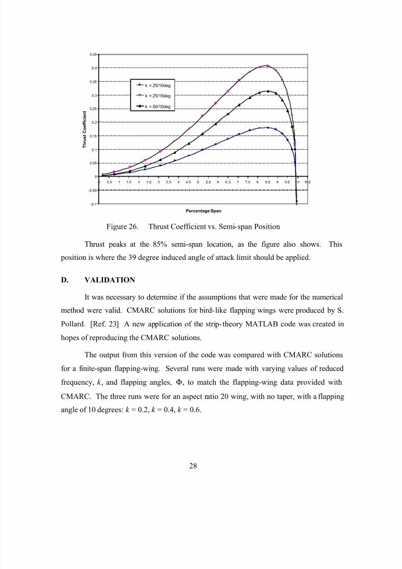
Because of 3-D effects, the wingtip is immersed in the wingtip vortex. Therefore
the limiting induced angle of attack occurs inboard along the span. The plot of CMARC
data for span-wise thrust coefficient distribution in Figure 26 illustrates this phenomenon.
7/18/2019 02Sep Randall
http://slidepdf.com/reader/full/02sep-randall 44/112
28
-0.1
-0.05
0
0.05
0.1
0.15
0.2
0.25
0.3
0.35
0.4
0.45
0 0.5 1 1.5 2 2.5 3 3.5 4 4.5 5 5.5 6 6.5 7 7.5 8 8.5 9 9.5 10 10.5
Percentage Span
T h r u s t C o e f f i c i e n t
k =.25/10deg
k =.25/15deg
k =.50/10deg
Figure 26. Thrust Coefficient vs. Semi-span Position
Thrust peaks at the 85% semi-span location, as the figure also shows. This
position is where the 39 degree induced angle of attack limit should be applied.
D. VALIDATION
It was necessary to determine if the assumptions that were made for the numericalmethod were valid. CMARC solutions for bird-like flapping wings were produced by S.
Pollard. [Ref. 23] A new application of the strip- theory MATLAB code was created in
hopes of reproducing the CMARC solutions.
The output from this version of the code was compared with CMARC solutions
for a finite-span flapping-wing. Several runs were made with varying values of reduced
frequency, k , and flapping angles, Φ, to match the flapping-wing data provided with
CMARC. The three runs were for an aspect ratio 20 wing, with no taper, with a flappingangle of 10 degrees: k = 0.2, k = 0.4, k = 0.6.
7/18/2019 02Sep Randall
http://slidepdf.com/reader/full/02sep-randall 45/112
29
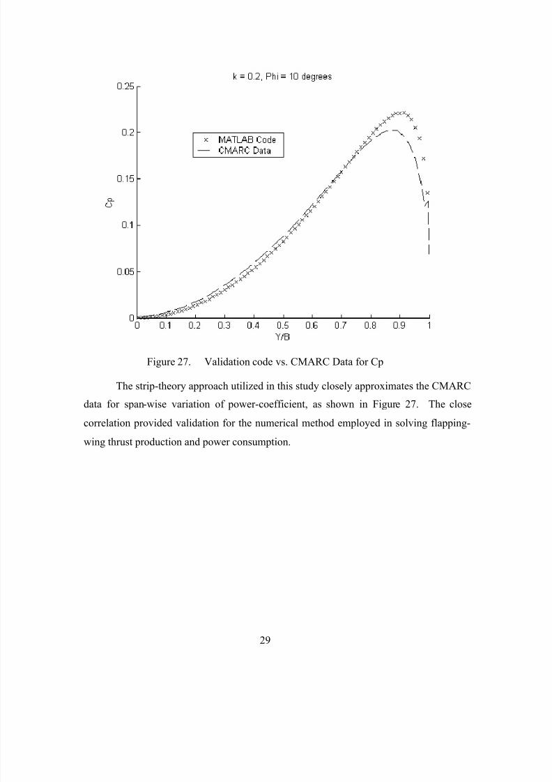
Figure 27. Validation code vs. CMARC Data for Cp
The strip-theory approach utilized in this study closely approximates the CMARC
data for span-wise variation of power-coefficient, as shown in Figure 27. The close
correlation provided validation for the numerical method employed in solving flapping-
wing thrust production and power consumption.
7/18/2019 02Sep Randall
http://slidepdf.com/reader/full/02sep-randall 46/112
30
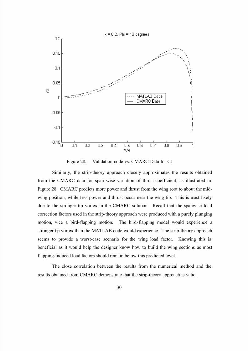
Figure 28. Validation code vs. CMARC Data for Ct
Similarly, the strip-theory approach closely approximates the results obtained
from the CMARC data for span wise variation of thrust-coefficient, as illustrated in
Figure 28. CMARC predicts more power and thrust from the wing root to about the mid-
wing position, while less power and thrust occur near the wing tip. This is most likely
due to the stronger tip vortex in the CMARC solution. Recall that the spanwise load
correction factors used in the strip-theory approach were produced with a purely plunging
motion, vice a bird-flapping motion. The bird-flapping model would experience a
stronger tip vortex than the MATLAB code would experience. The strip-theory approach
seems to provide a worst-case scenario for the wing load factor. Knowing this is
beneficial as it would help the designer know how to build the wing sections as most
flapping-induced load factors should remain below this predicted level.
The close correlation between the results from the numerical method and the
results obtained from CMARC demonstrate that the strip-theory approach is valid.
7/18/2019 02Sep Randall
http://slidepdf.com/reader/full/02sep-randall 47/112
31
III. RESULTS
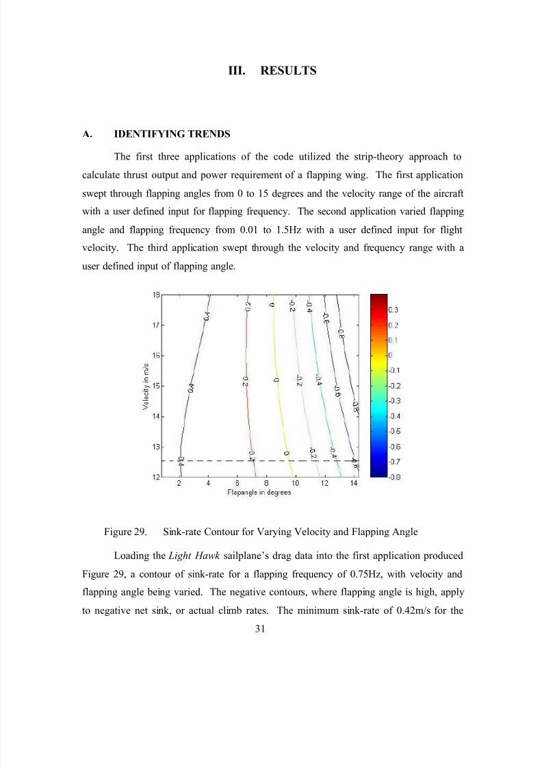
A. IDENTIFYING TRENDS
The first three applications of the code utilized the strip-theory approach to
calculate thrust output and power requirement of a flapping wing. The first application
swept through flapping angles from 0 to 15 degrees and the velocity range of the aircraft
with a user defined input for flapping frequency. The second application varied flapping
angle and flapping frequency from 0.01 to 1.5Hz with a user defined input for flight
velocity. The third application swept through the velocity and frequency range with a
user defined input of flapping angle.
Figure 29. Sink-rate Contour for Varying Velocity and Flapping Angle
Loading the Light Hawk sailplane’s drag data into the first application produced
Figure 29, a contour of sink-rate for a flapping frequency of 0.75Hz, with velocity and
flapping angle being varied. The negative contours, where flapping angle is high, apply
to negative net sink, or actual climb rates. The minimum sink-rate of 0.42m/s for the
7/18/2019 02Sep Randall
http://slidepdf.com/reader/full/02sep-randall 48/112
32
base Light Hawk aircraft occurs at a velocity of 12.5m/s, and is designated by the dashed
horizontal line in the plot. As the flapping angle nears zero, thrust approaches zero, and
the minimum sink velocity approaches the original minimum sink velocity of 12.5m/s.
As the flapping angle increases the flapping amplitude, h, increases. The contour lines
become closely spaced at the higher flapping angles, meaning that increased thrust is
offsetting the sink-rate more effectively. This agrees well with 2-D theory where thrust
increases as the flapping amplitude squared. The larger the flapping angle, the more
beneficial it is to fly at higher velocities. Be aware this trend pays no heed to what the
power requirement is.
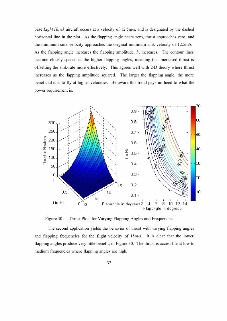
Figure 30. Thrust Plots for Varying Flapping Angles and Frequencies
The second application yields the behavior of thrust with varying flapping angles
and flapping frequencies for the flight velocity of 15m/s. It is clear that the lower
flapping angles produce very little benefit, in Figure 30. The thrust is accessible at low to
medium frequencies where flapping angles are high.
7/18/2019 02Sep Randall
http://slidepdf.com/reader/full/02sep-randall 49/112
33
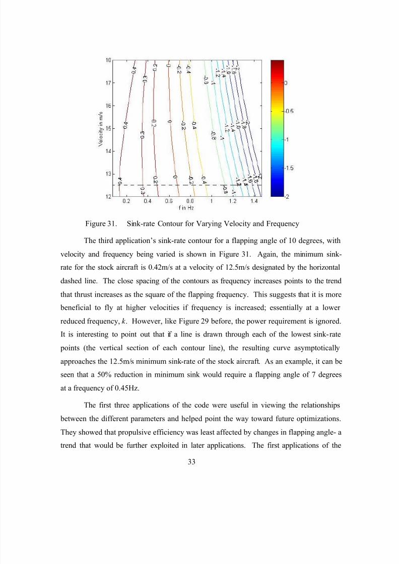
Figure 31. Sink-rate Contour for Varying Velocity and Frequency
The third application’s sink-rate contour for a flapping angle of 10 degrees, with
velocity and frequency being varied is shown in Figure 31. Again, the minimum sink-
rate for the stock aircraft is 0.42m/s at a velocity of 12.5m/s designated by the horizontal
dashed line. The close spacing of the contours as frequency increases points to the trend
that thrust increases as the square of the flapping frequency. This suggests that it is more beneficial to fly at higher velocities if frequency is increased; essentially at a lower
reduced frequency, k . However, like Figure 29 before, the power requirement is ignored.
It is interesting to point out that if a line is drawn through each of the lowest sink-rate
points (the vertical section of each contour line), the resulting curve asymptotically
approaches the 12.5m/s minimum sink-rate of the stock aircraft. As an example, it can be
seen that a 50% reduction in minimum sink would require a flapping angle of 7 degrees
at a frequency of 0.45Hz.
The first three applications of the code were useful in viewing the relationships
between the different parameters and helped point the way toward future optimizations.
They showed that propulsive efficiency was least affected by changes in flapping angle- a
trend that would be further exploited in later applications. The first applications of the
7/18/2019 02Sep Randall
http://slidepdf.com/reader/full/02sep-randall 50/112
34
code suggest that propulsive efficiency increases at higher velocities. Recalling equation
(1), efficiency increases as reduced frequency, k , decreases.
2 fck
U
π= (1)
To make k as small as possible, it is necessary to increase velocity, decrease
flapping frequency, and decrease chord length. This agrees with theory, where efficiency
asymptotically approaches 100% as k goes to 0. [Ref. 17]
B. CONSTRAINTS
An improved application of the code was produced that included an iterative
method for finding the maximum thrust available given a user-specified power constraint.
Since the aircraft are limited by human power output (200W), what parameters could beoptimized to maximize thrust? As mentioned earlier, propulsive efficiency was least
affected by changes in flapping angle. In addition, flapping angle is not tied to the
structure of the airframe. The constraining code used the secant method to determine the
flapping angle that would satisfy the specified power restriction as velocity and flapping
frequency were varied. As velocity increased, the allowable flap angle for a given
frequency decreased, likewise, at lower velocities large flap angles were allowed with
higher frequencies. An illustration of how this works is shown in Figure 32, where the
power plateaus at the specified power restriction of 1250W.
7/18/2019 02Sep Randall
http://slidepdf.com/reader/full/02sep-randall 51/112
35
Figure 32. Specified Power Restriction of 1250W
The wing is free to move at the maximum flapping angle of 15 degrees until the
power requirement reaches 1250W as shown by the plateau on the left. On the right, this
corresponds to the rise of the power requirement as the flapping frequency increases for
the given flapping angle of 15 degrees. When the power constraint is met, the flapping
angle is curtailed to keep the power requirement at the limit. The power plateau on the
right corresponds to the decrease in flapping angle to the left.
The constraining code was subsequently tailored to the three aircraft
configurations in this study: the human-powered SparrowHawk and Light Hawk
applications included aircraft-specific drag-polar data that was obtained from the
respective manufacturers. In addition, the flight velocities, flapping frequencies, and
flapping angles were tailored for the aircraft. The final aircraft was an electric-powered
sustainer version of the Light Hawk sailplane. The guideline for the sustainer system is to
arrest sink-rate and provide for a maximum 0.85m/s climb rate. As noted earlier, after
losses were considered, the Light Hawk aircraft required 2875W to meet the criteria. The
sustainer application found the most efficient means of thrust production using a 2875W
imbedded power restriction.
7/18/2019 02Sep Randall
http://slidepdf.com/reader/full/02sep-randall 52/112
36
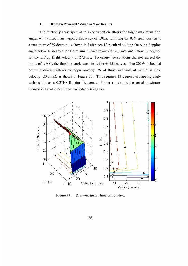
1. Human-Powered SparrowHawk Results
The relatively short span of this configuration allows for larger maximum flap
angles with a maximum flapping frequency of 1.0Hz. Limiting the 85% span location to
a maximum of 39 degrees as shown in Reference 12 required holding the wing flappingangle below 16 degrees for the minimum sink velocity of 20.5m/s, and below 19 degrees
for the L/Dmax flight velocity of 27.9m/s. To ensure the solutions did not exceed the
limits of UPOT, the flapping angle was limited to +/-15 degrees. The 200W imbedded
power restriction allows for approximately 9N of thrust available at minimum sink
velocity (20.5m/s), as shown in Figure 33. This requires 13 degrees of flapping angle
with as low as a 0.25Hz flapping frequency. Under constraints the actual maximum
induced angle of attack never exceeded 9.6 degrees.
Figure 33. SparrowHawk Thrust Production
7/18/2019 02Sep Randall
http://slidepdf.com/reader/full/02sep-randall 53/112
37
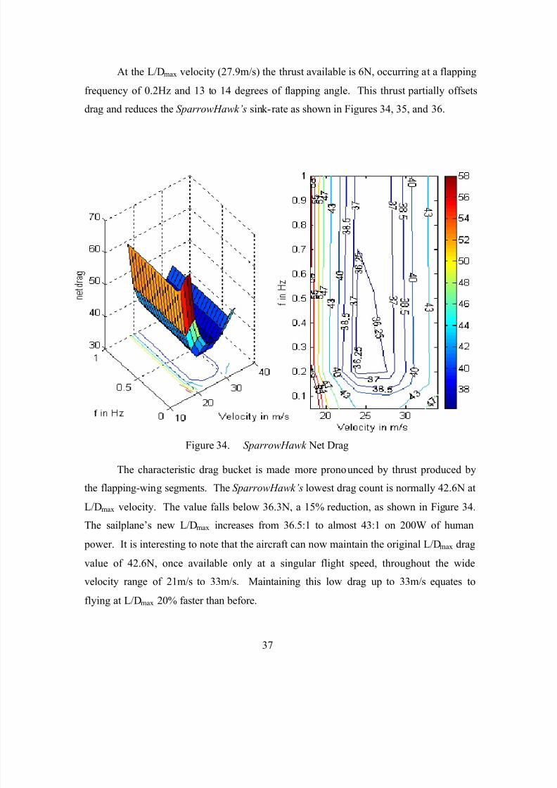
At the L/Dmax velocity (27.9m/s) the thrust available is 6N, occurring at a flapping
frequency of 0.2Hz and 13 to 14 degrees of flapping angle. This thrust partially offsets
drag and reduces the SparrowHawk’s sink-rate as shown in Figures 34, 35, and 36.
Figure 34. SparrowHawk Net Drag
The characteristic drag bucket is made more pronounced by thrust produced by
the flapping-wing segments. The SparrowHawk’s lowest drag count is normally 42.6N at
L/Dmax velocity. The value falls below 36.3N, a 15% reduction, as shown in Figure 34.
The sailplane’s new L/Dmax increases from 36.5:1 to almost 43:1 on 200W of human
power. It is interesting to note that the aircraft can now maintain the original L/Dmax drag
value of 42.6N, once available only at a singular flight speed, throughout the wide
velocity range of 21m/s to 33m/s. Maintaining this low drag up to 33m/s equates to
flying at L/Dmax 20% faster than before.
7/18/2019 02Sep Randall
http://slidepdf.com/reader/full/02sep-randall 54/112
38
8
12
16
20
24
28
32
36
40
44
16 20 24 28 32 36 40 44 48 52 56 60 64 68
Velocity (m/s)
L / D
oldL/D
newL/D
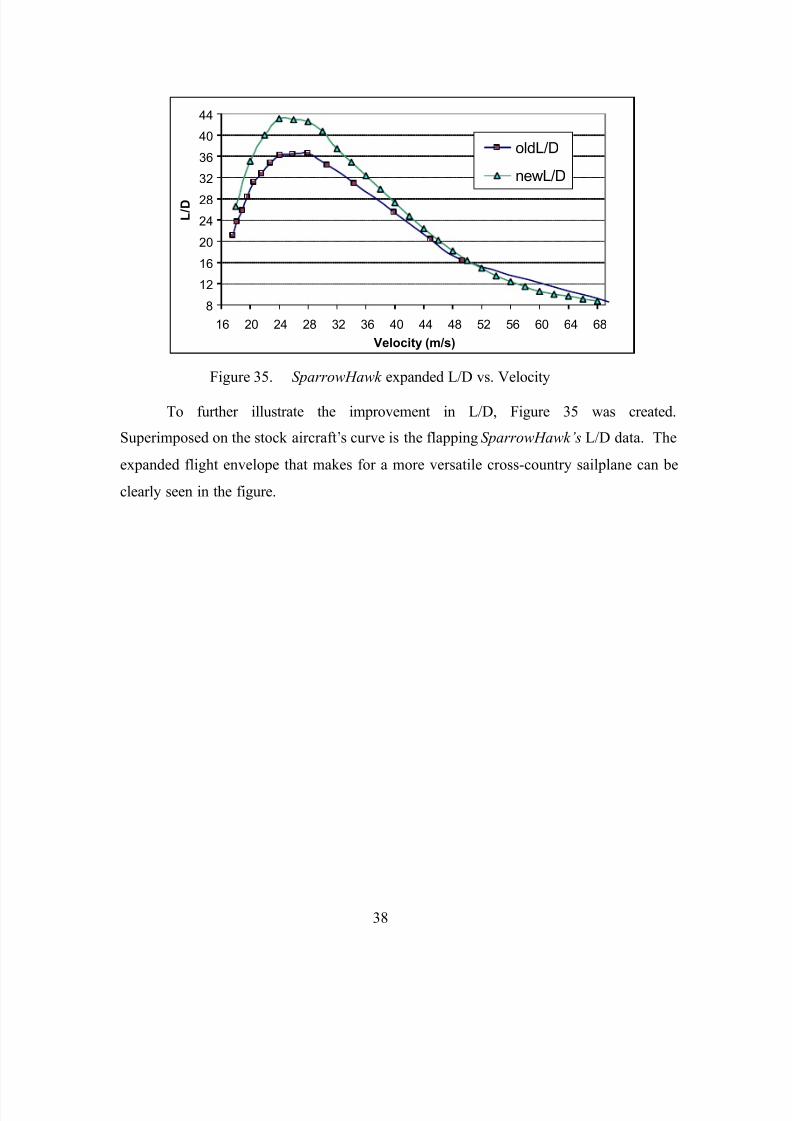
Figure 35. SparrowHawk expanded L/D vs. Velocity
To further illustrate the improvement in L/D, Figure 35 was created.
Superimposed on the stock aircraft’s curve is the flapping SparrowHawk’s L/D data. The
expanded flight envelope that makes for a more versatile cross-country sailplane can be
clearly seen in the figure.
7/18/2019 02Sep Randall
http://slidepdf.com/reader/full/02sep-randall 55/112
39
Figure 36. SparrowHawk Sink Rate
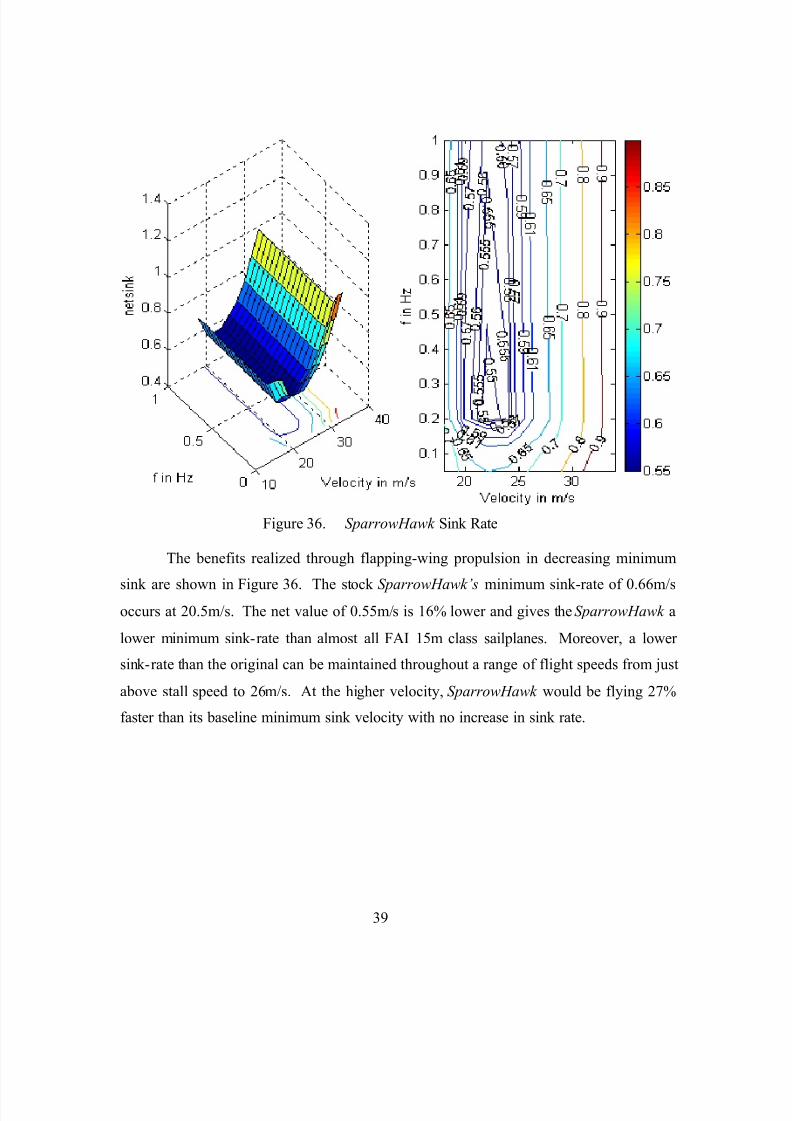
The benefits realized through flapping-wing propulsion in decreasing minimum
sink are shown in Figure 36. The stock SparrowHawk’s minimum sink-rate of 0.66m/soccurs at 20.5m/s. The net value of 0.55m/s is 16% lower and gives the SparrowHawk a
lower minimum sink-rate than almost all FAI 15m class sailplanes. Moreover, a lower
sink-rate than the original can be maintained throughout a range of flight speeds from just
above stall speed to 26m/s. At the higher velocity, SparrowHawk would be flying 27%
faster than its baseline minimum sink velocity with no increase in sink rate.
7/18/2019 02Sep Randall
http://slidepdf.com/reader/full/02sep-randall 56/112
40
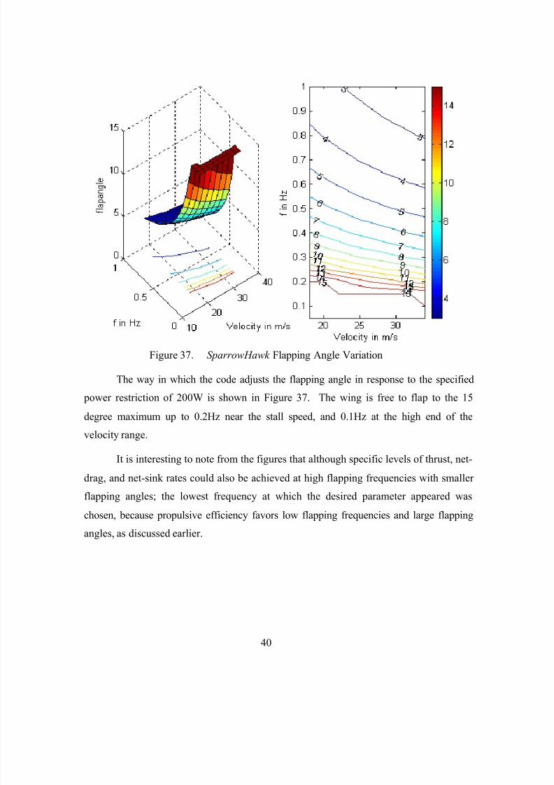
Figure 37. SparrowHawk Flapping Angle Variation
The way in which the code adjusts the flapping angle in response to the specified
power restriction of 200W is shown in Figure 37. The wing is free to flap to the 15
degree maximum up to 0.2Hz near the stall speed, and 0.1Hz at the high end of the
velocity range.
It is interesting to note from the figures that although specific levels of thrust, net-
drag, and net-sink rates could also be achieved at high flapping frequencies with smaller
flapping angles; the lowest frequency at which the desired parameter appeared was
chosen, because propulsive efficiency favors low flapping frequencies and large flapping
angles, as discussed earlier.
7/18/2019 02Sep Randall
http://slidepdf.com/reader/full/02sep-randall 57/112
41
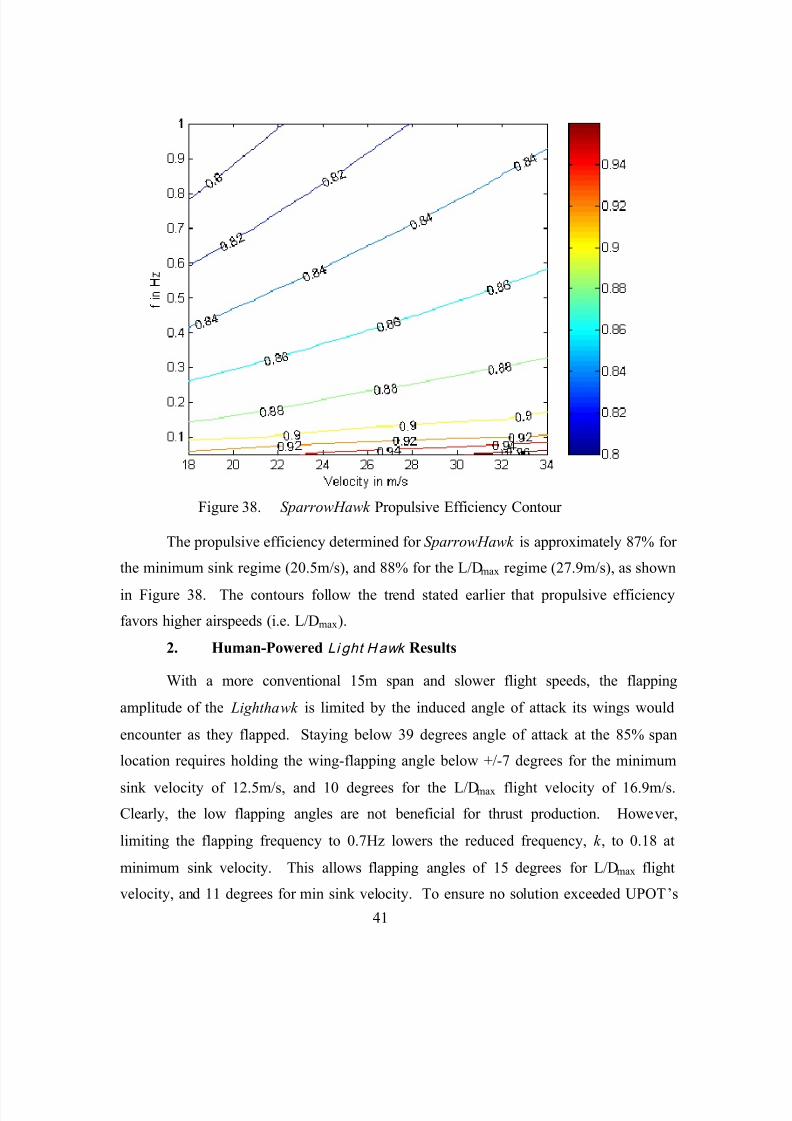
Figure 38. SparrowHawk Propulsive Efficiency Contour
The propulsive efficiency determined for SparrowHawk is approximately 87% for
the minimum sink regime (20.5m/s), and 88% for the L/Dmax regime (27.9m/s), as shown
in Figure 38. The contours follow the trend stated earlier that propulsive efficiency
favors higher airspeeds (i.e. L/Dmax).
2. Human-Powered Li ght Hawk Results
With a more conventional 15m span and slower flight speeds, the flapping
amplitude of the Lighthawk is limited by the induced angle of attack its wings would
encounter as they flapped. Staying below 39 degrees angle of attack at the 85% span
location requires holding the wing-flapping angle below +/-7 degrees for the minimum
sink velocity of 12.5m/s, and 10 degrees for the L/Dmax flight velocity of 16.9m/s.
Clearly, the low flapping angles are not beneficial for thrust production. However,
limiting the flapping frequency to 0.7Hz lowers the reduced frequency, k , to 0.18 at
minimum sink velocity. This allows flapping angles of 15 degrees for L/Dmax flight
velocity, and 11 degrees for min sink velocity. To ensure no solution exceeded UPOT’s
7/18/2019 02Sep Randall
http://slidepdf.com/reader/full/02sep-randall 58/112
42
limits, the code was run with +/-10 degrees where maximum expected αi at the 85% span
location is 38 degrees. Under constraints the maximum induced angle of attack never
exceeded 12.6 degrees.
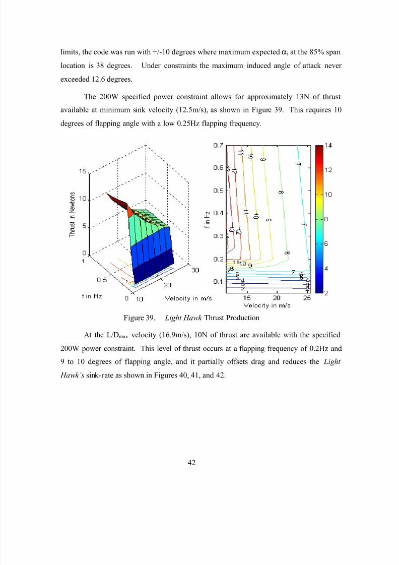
The 200W specified power constraint allows for approximately 13N of thrustavailable at minimum sink velocity (12.5m/s), as shown in Figure 39. This requires 10
degrees of flapping angle with a low 0.25Hz flapping frequency.
Figure 39. Light Hawk Thrust Production
At the L/Dmax velocity (16.9m/s), 10N of thrust are available with the specified
200W power constraint. This level of thrust occurs at a flapping frequency of 0.2Hz and
9 to 10 degrees of flapping angle, and it partially offsets drag and reduces the Light
Hawk’s sink-rate as shown in Figures 40, 41, and 42.
7/18/2019 02Sep Randall
http://slidepdf.com/reader/full/02sep-randall 59/112
43
Figure 40. Light Hawk Drag Reduction
The Light Hawk’s lowest drag force is normally 44.3N at L/Dmax velocity
(16.9m/s). Under human power, the value falls below 35.5N, a 20% reduction, as shown
in Figure 40. The sailplane’s new L/Dmax increases from 35:1 to 41.8:1 on 200W of
human power. The aircraft can now maintain its original L/Dmax drag value of 44.3N,
once available only at a singular flight speed, from just above stall speed to 23m/s. At
23m/s, the aircraft would be flying 36% faster than its original L/Dmax velocity with the
same low drag value.
7/18/2019 02Sep Randall
http://slidepdf.com/reader/full/02sep-randall 60/112
44
14
18
22
26
30
34
38
42
10 12 14 16 18 20 22 24 26 28 30 32 34 36 38 40Velocity (m/s)
L / D
oldL/D
newL/D
Figure 41. Light Hawk Expanded L/D vs. Velocity
The improvement in L/D is clearly shown in Figure 41. The new L/D data is
superimposed on the stock aircraft’s curve showing the flapping Light Hawk’s expanded
flight envelope. With the increase in L/D at the higher velocities, the aircraft would have
improved cross-country potential.
7/18/2019 02Sep Randall
http://slidepdf.com/reader/full/02sep-randall 61/112
45
Figure 42. Light Hawk Sink Rate
The stock Light Hawk’s benchmark minimum sink-rate of 0.42m/s at 12.5m/s is
matched only by three open class sailplanes with wingspans greater than 24.5m. The net
value of 0.32m/s, shown in Figure 42, lowers the sink-rate an additional 24%. No other
sailplane, let alone bird or winged mammal, can match this sink rate. Moreover, sink
rates lower than the stock aircraft can be maintained from just above stall speed to
17.5m/s. At the higher velocity, Light Hawk would be flying 40% faster than its baseline
minimum sink velocity with no increase in sink rate.
7/18/2019 02Sep Randall
http://slidepdf.com/reader/full/02sep-randall 62/112
46
Figure 43. Light Hawk Flapping Angle Variation
The way in which the flapping angle is tailored to conform to the 200W power
constraint is shown in Figure 43. The wing is free to flap to the 10 degree maximum up
to 0.2Hz near the stall speed, and 0.1Hz at the high end of the velocity range. The most
useful flapping angles vary from 9.5 degrees to 8 degrees at a flapping frequency of
0.2Hz.
7/18/2019 02Sep Randall
http://slidepdf.com/reader/full/02sep-randall 63/112
47
Figure 44. Light Hawk Propulsive Efficiency
The variation in propulsive efficiency throughout the velocity and flapping
frequency ranges is shown in Figure 44. Propulsive efficiency varies from 85% to 86%
depending on flight velocity at minimum sink or L/Dmax.3. Sustainer Results
The sustainer system is modeled around the Light Hawk aircraft. The code was
run using a specified power constraint of 2875W, the amount required to arrest sink-rate
and provide for a 0.85m/s rate of climb.
7/18/2019 02Sep Randall
http://slidepdf.com/reader/full/02sep-randall 64/112
48
Figure 45. Sustainer Thrust Production
The highest thrust levels are achievable at low flight velocities, as shown in
Figure 45. This is similar in behavior to propeller thrust production, where static thrust is
the highest value, and increases in airspeed cause a reduction in thrust due to the decrease
in induced blade pitch angles.
7/18/2019 02Sep Randall
http://slidepdf.com/reader/full/02sep-randall 65/112
49
Figure 46. Sustainer Net Drag
Negative contour lines indicate thrust is greater than drag, as shown in Figure 46.
The thrust required to arrest sink-rate for a Light Hawk is 45N, represented by the net
drag contour line of zero. The sustainer produces sufficient thrust throughout the Light
Hawk’s flight speed envelope to arrest sink rate. Flying along the zero contour line
essentially provides the Light Hawk with an L/D of infinity; of interest for pilots using
the system to “buy time” to search for better conditions while minimizing the power drain
on the batteries. The power requirement of flying along this contour line varies from
700W at 15m/s up to 1800W at 31m/s.
7/18/2019 02Sep Randall
http://slidepdf.com/reader/full/02sep-randall 66/112
50
Figure 47. Sustainer Climb and Sink Rates
The performance goal of the sustainer aircraft is a climb rate of 0.85m/s. This is
available from a flapping frequency of 0.68Hz at a flight velocity of 19m/s, as shown in
Figure 47. The zero sink-rate contour, where sink-rate is arrested, occurs as low as 0.4Hz
at a flight speed of 16m/s.
7/18/2019 02Sep Randall
http://slidepdf.com/reader/full/02sep-randall 67/112
51
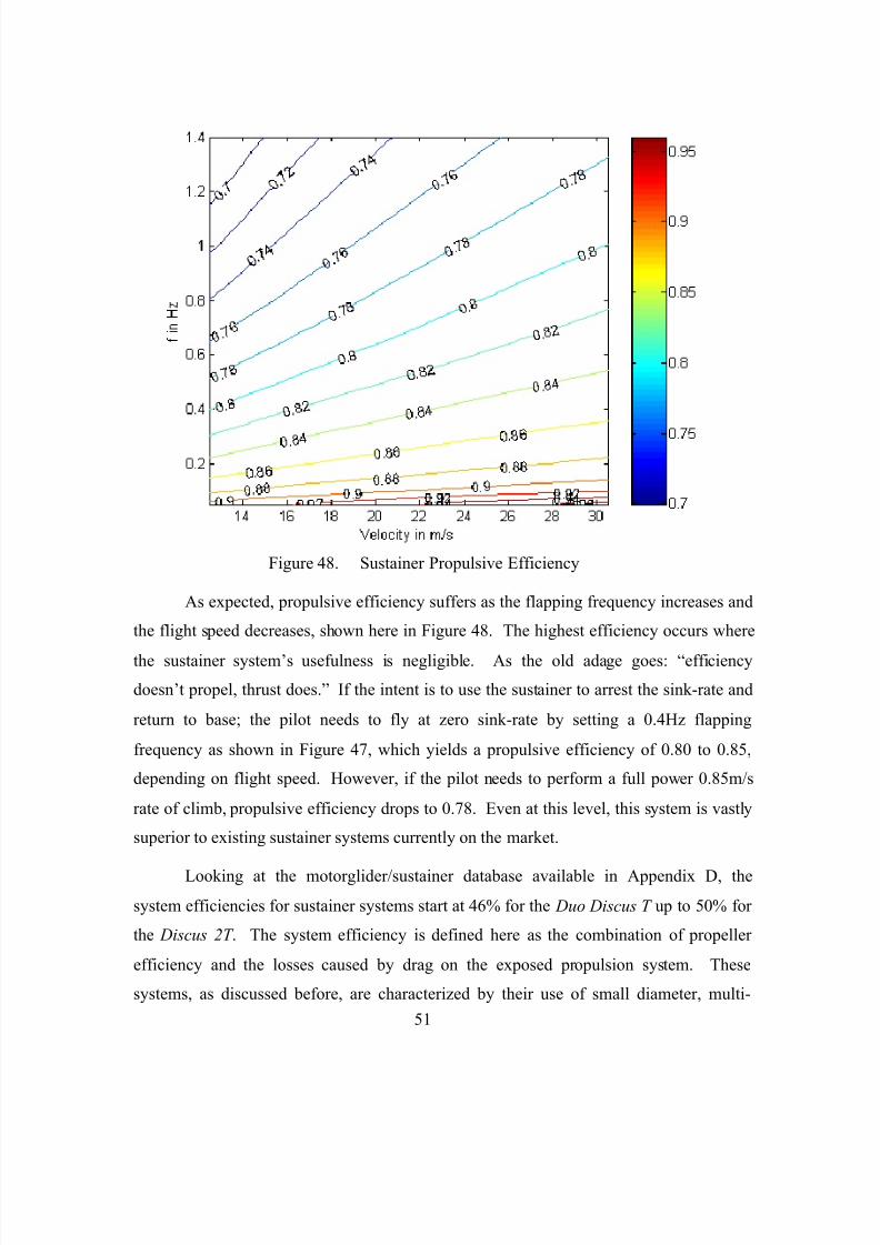
Figure 48. Sustainer Propulsive Efficiency
As expected, propulsive efficiency suffers as the flapping frequency increases and
the flight speed decreases, shown here in Figure 48. The highest efficiency occurs where
the sustainer system’s usefulness is negligible. As the old adage goes: “efficiency
doesn’t propel, thrust does.” If the intent is to use the sustainer to arrest the sink-rate and
return to base; the pilot needs to fly at zero sink-rate by setting a 0.4Hz flapping
frequency as shown in Figure 47, which yields a propulsive efficiency of 0.80 to 0.85,
depending on flight speed. However, if the pilot needs to perform a full power 0.85m/s
rate of climb, propulsive efficiency drops to 0.78. Even at this level, this system is vastly
superior to existing sustainer systems currently on the market.
Looking at the motorglider/sustainer database available in Appendix D, the
system efficiencies for sustainer systems start at 46% for the Duo Discus T up to 50% for
the Discus 2T . The system efficiency is defined here as the combination of propeller
efficiency and the losses caused by drag on the exposed propulsion system. These
systems, as discussed before, are characterized by their use of small diameter, multi-
7/18/2019 02Sep Randall
http://slidepdf.com/reader/full/02sep-randall 68/112
52
bladed propellers. The propulsive systems’ motors consist of small two-stroke units that
produce best power at 5750-6500 rpm. The propellers are direct-drive, or with small
reduction gearing, thus they turn at very high speeds that decrease efficiency. In
addition, the multiple blades cause interference losses that further decrease propeller
efficiency.
The system efficiency for a Light Hawk based sustainer consists of the propulsive
efficiency, stated above as varying between 78% and 85% depending on flight speed, and
mechanical losses, estimated at 5%. The total system efficiency for the flapping-wing
sustainer would vary between 74.1% and 80.8%, dependent on flight speed- a significant
increase from the Discus’ 46% to 50%.
7/18/2019 02Sep Randall
http://slidepdf.com/reader/full/02sep-randall 69/112
53
IV. CONCLUSIONS
In this paper, flapping-wing propulsion as a means of drag reduction was
investigated numerically. This study was conducted with the hope that the inherent
flexibility of high aspect ratio sailplane wings could be harnessed to flap at their natural
frequencies.
The numerical method used a strip-theory approach, applying 3-D corrections to
2-D data. Thrust and power coefficients were computed for flapping-wing sections.
Spanwise load factors were applied to calculate total wing thrust production and power
consumption. The approach was deemed suitable as results from this numerical method
compared favorably with established CMARC 3-D results.
New applications of the method were used to determine trends in thrust and
power coefficients with changes in velocity, flapping angle, and flapping frequency
parameters. With the information acquired from these results, a constraining code was
written to determine what combinations of these parameters would provide for the
highest thrust given specified power constraints.
The results of these aircraft-tailored constraining codes clearly show that marked
improvements in minimum sink and L/Dmax performance parameters for ultralight
sailplanes are possible by means of human-powered flapping-wing propulsion.
Theoretical decreases in minimum sink are 16% for the SparrowHawk , and 24% for the
Light Hawk sailplanes. Likewise, L/Dmax may also be improved 15% from 36.5:1 to 42:1,
and 20% from 35:1 to 41.8:1, respectively. These gains in performance would be
possible with high propulsive efficiencies in the 85% to 88% range.
The Light Hawk -based sustainer system can arrest sink-rate and provide for a
0.85m/s rate of climb using just 2875W (3.9bhp). In addition, zero sink-rate can be
maintained throughout the Light Hawk’s flight envelope from as low as 700W (0.94bhp).
These results come with a favorable propulsive efficiency range of 78% to 85%, and total
system efficiencies of 74.1% to 80.8%, depending on flight speed.

7/18/2019 02Sep Randall
http://slidepdf.com/reader/full/02sep-randall 70/112
54
THIS PAGE INTENTIONALLY LEFT BLANK
7/18/2019 02Sep Randall
http://slidepdf.com/reader/full/02sep-randall 71/112
55
V. RECOMMENDATIONS
Using 2-D panel-code data in a strip-theory approach allows for a rather
inexpensive means of studying flapping-wing propulsion. There are virtually endless
flapping-wing configurations and parameters where this numerical method could be
applied. This study concerned itself with limited power applications to offset airframe
drag. To further probe in this direction, more time could be spent studying the extreme
cases: low frequency with large flapping angle propulsion, and high frequency with small
flapping angle propulsion. Perhaps a combination could be applied to drag reduction in
large commercial aircraft surfaces.
From a numerical analysis view, more time could be spent refining the method toinvestigate both plunging and pitching airfoil motions. The task is a daunting one, as it
would require interpolating data from 4-D matrices that would include: plunge amplitude,
pitch amplitude, phase, and frequency.
From a structural standpoint, ways of tuning the natural frequency of wings to
desired levels could be studied. By giving control of this parameter to the pilot, the
aircraft flight envelope need not be restricted to avoid flutter. Perhaps it is not necessary.
Maybe high aspect ratio, flexible wings with fixed low natural frequencies can besufficiently controlled at higher flight speeds through active controls (i.e. fly-by-wire).
Obviously, more time could be spent refining the flapping mechanism. A wind-
tunnel model would help verify the numerical results experimentally. A flying model of
a sustainer system would also be beneficial.

7/18/2019 02Sep Randall
http://slidepdf.com/reader/full/02sep-randall 72/112
56
THIS PAGE INTENTIONALLY LEFT BLANK
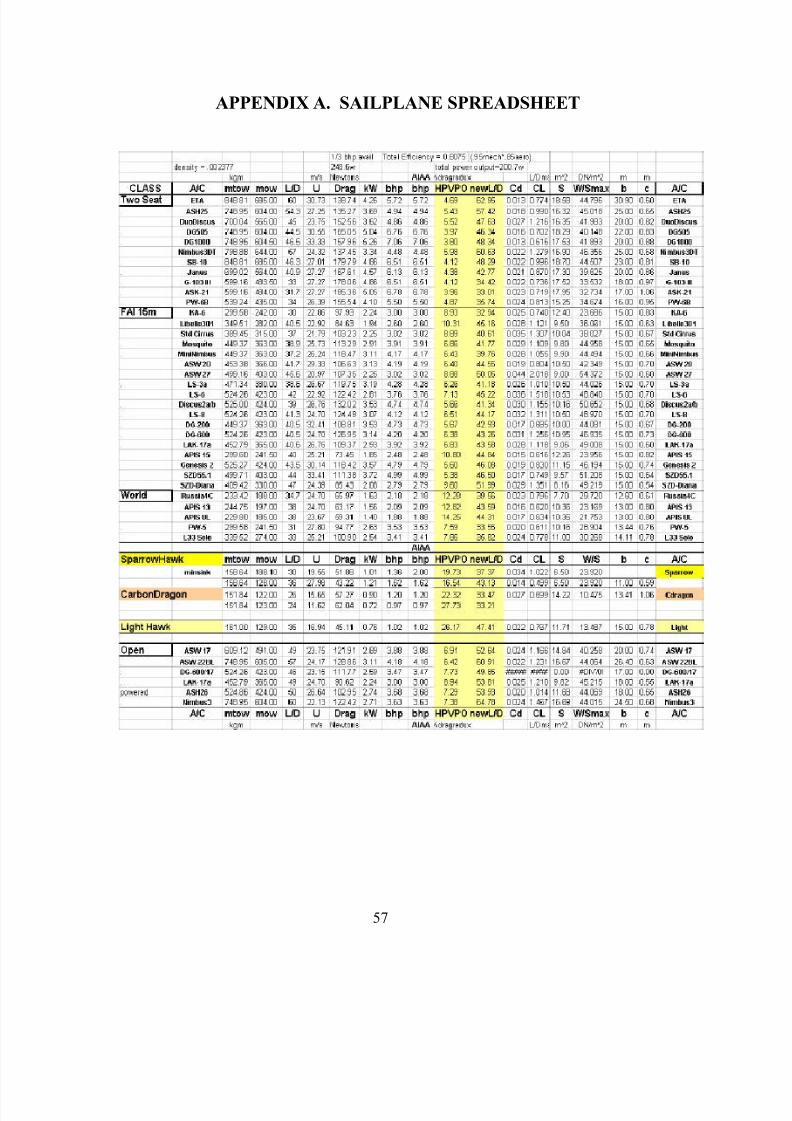
7/18/2019 02Sep Randall
http://slidepdf.com/reader/full/02sep-randall 73/112
57
APPENDIX A. SAILPLANE SPREADSHEET
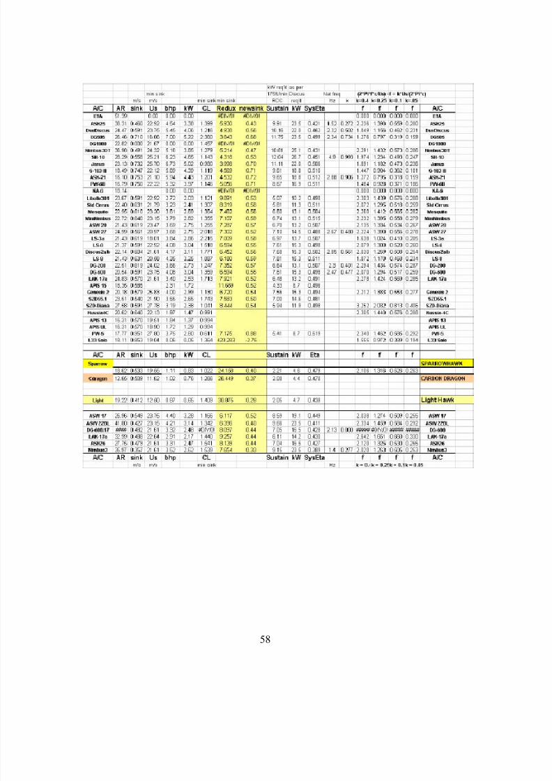
7/18/2019 02Sep Randall
http://slidepdf.com/reader/full/02sep-randall 74/112
58
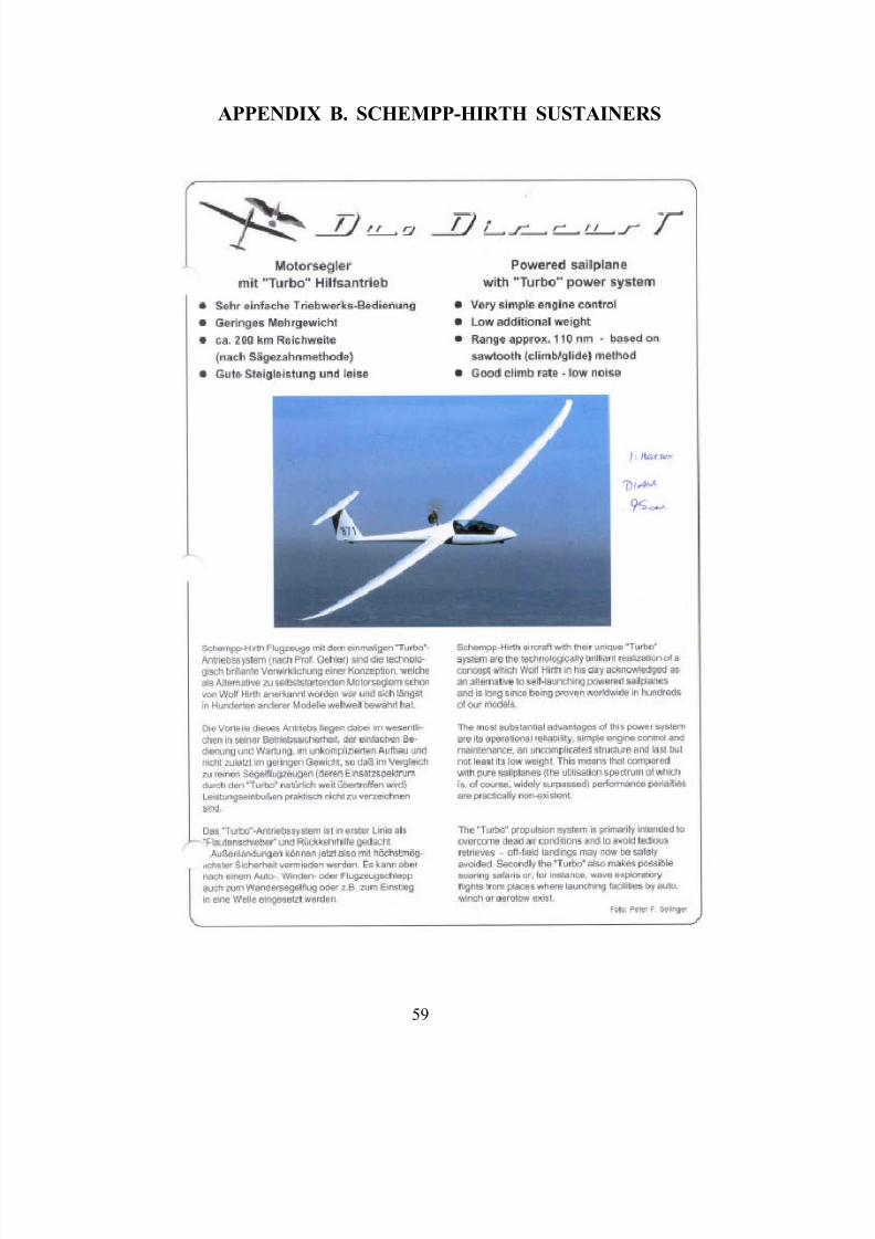
7/18/2019 02Sep Randall
http://slidepdf.com/reader/full/02sep-randall 75/112
59
APPENDIX B. SCHEMPP-HIRTH SUSTAINERS
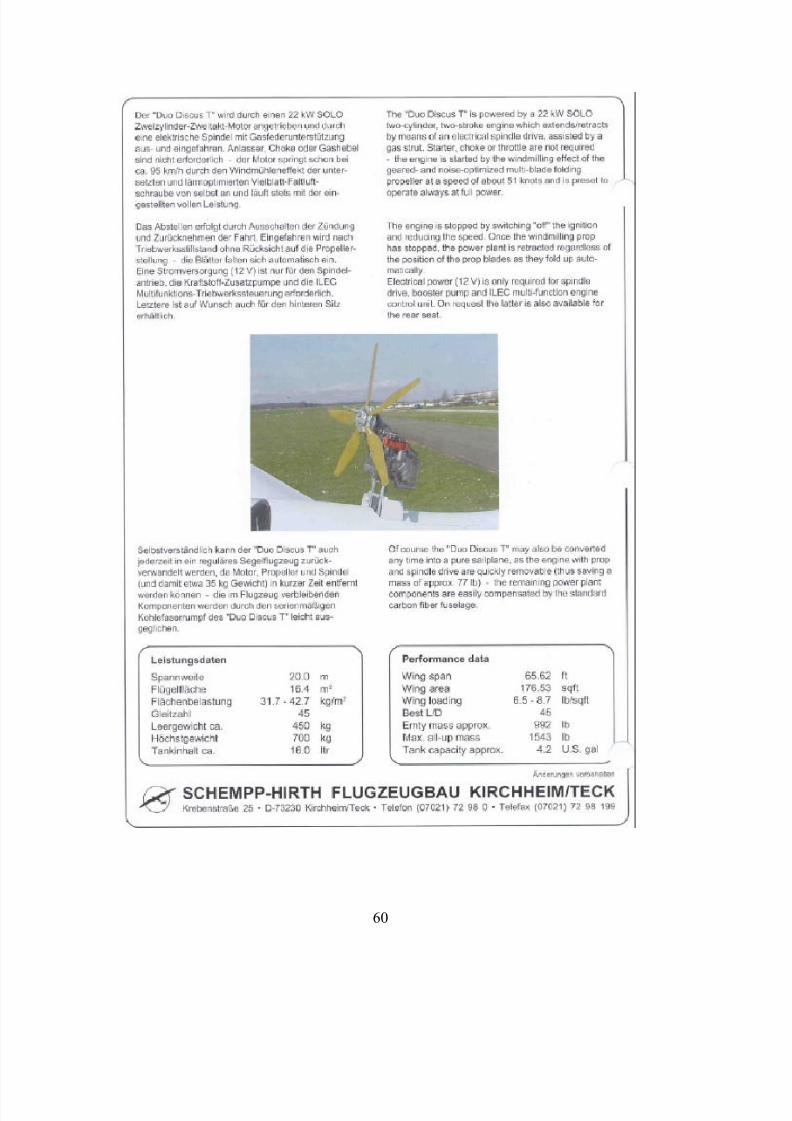
7/18/2019 02Sep Randall
http://slidepdf.com/reader/full/02sep-randall 76/112
60
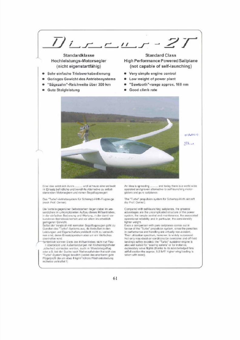
7/18/2019 02Sep Randall
http://slidepdf.com/reader/full/02sep-randall 77/112
61
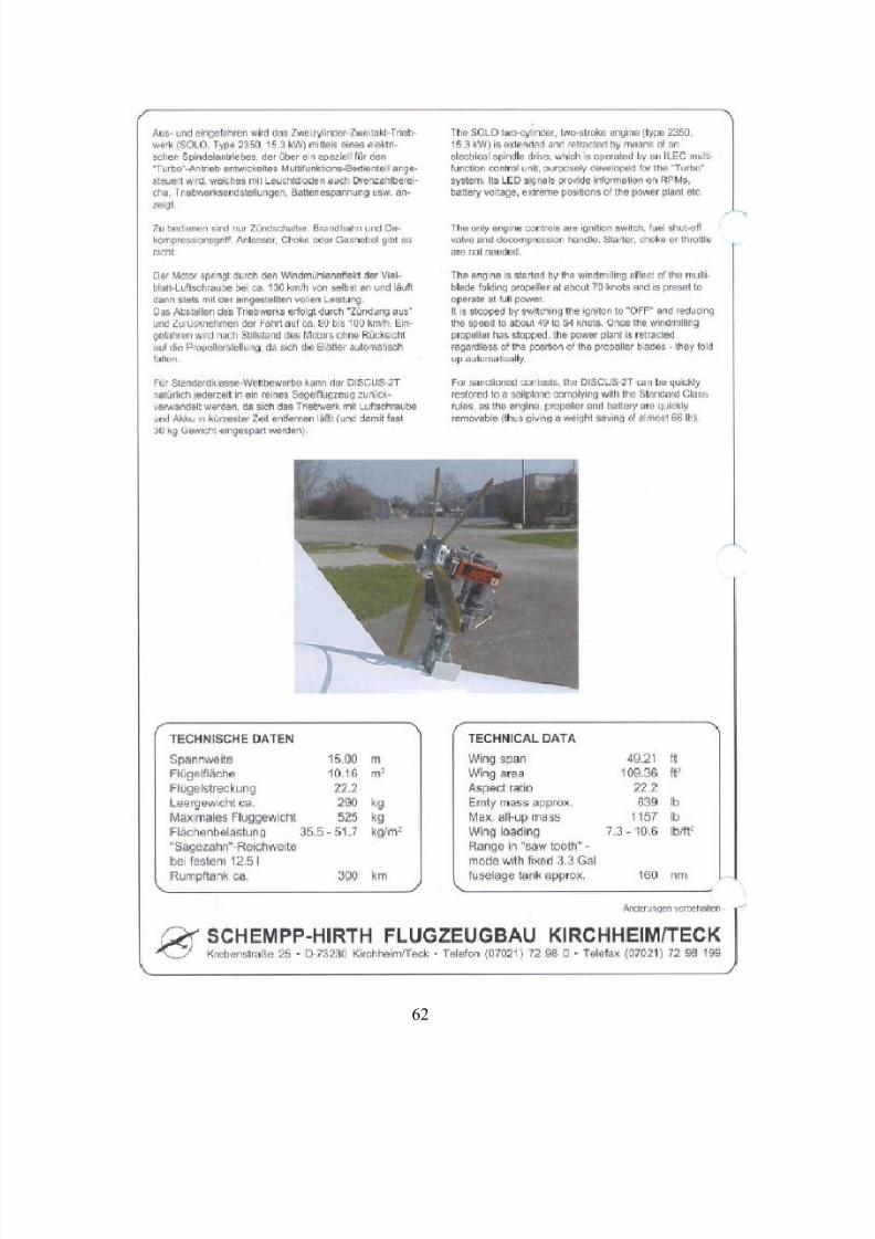
7/18/2019 02Sep Randall
http://slidepdf.com/reader/full/02sep-randall 78/112
62
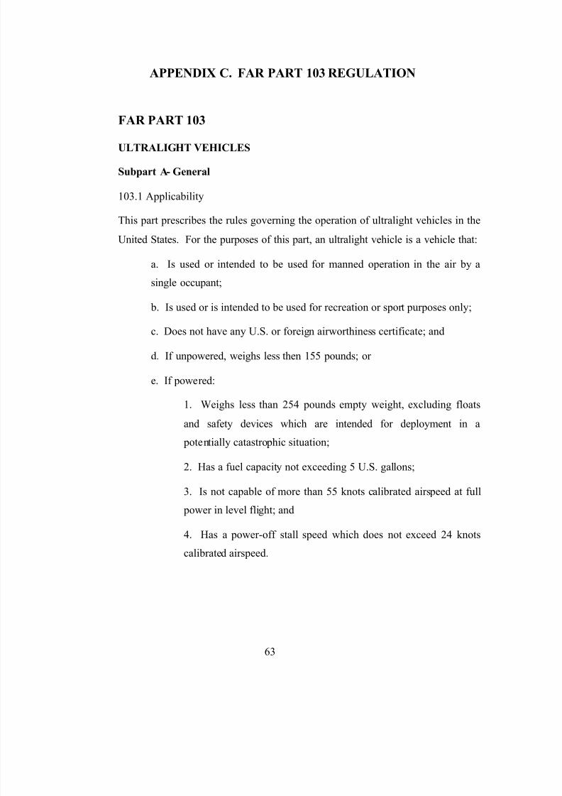
7/18/2019 02Sep Randall
http://slidepdf.com/reader/full/02sep-randall 79/112
63
APPENDIX C. FAR PART 103 REGULATION
FAR PART 103
ULTRALIGHT VEHICLES
Subpart A- General
103.1 Applicability
This part prescribes the rules governing the operation of ultralight vehicles in the
United States. For the purposes of this part, an ultralight vehicle is a vehicle that:
a. Is used or intended to be used for manned operation in the air by a
single occupant;
b. Is used or is intended to be used for recreation or sport purposes only;
c. Does not have any U.S. or foreign airworthiness certificate; and
d. If unpowered, weighs less then 155 pounds; or
e. If powered:
1. Weighs less than 254 pounds empty weight, excluding floats
and safety devices which are intended for deployment in a
potentially catastrophic situation;
2. Has a fuel capacity not exceeding 5 U.S. gallons;
3. Is not capable of more than 55 knots calibrated airspeed at full
power in level flight; and
4. Has a power-off stall speed which does not exceed 24 knots
calibrated airspeed.

7/18/2019 02Sep Randall
http://slidepdf.com/reader/full/02sep-randall 80/112
64
THIS PAGE INTENTIONALLY LEFT BLANK
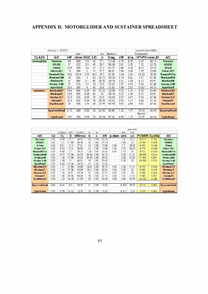
7/18/2019 02Sep Randall
http://slidepdf.com/reader/full/02sep-randall 81/112
65
APPENDIX D. MOTORGLIDER AND SUSTAINER SPREADSHEET

7/18/2019 02Sep Randall
http://slidepdf.com/reader/full/02sep-randall 82/112
66
THIS PAGE INTENTIONALLY LEFT BLANK
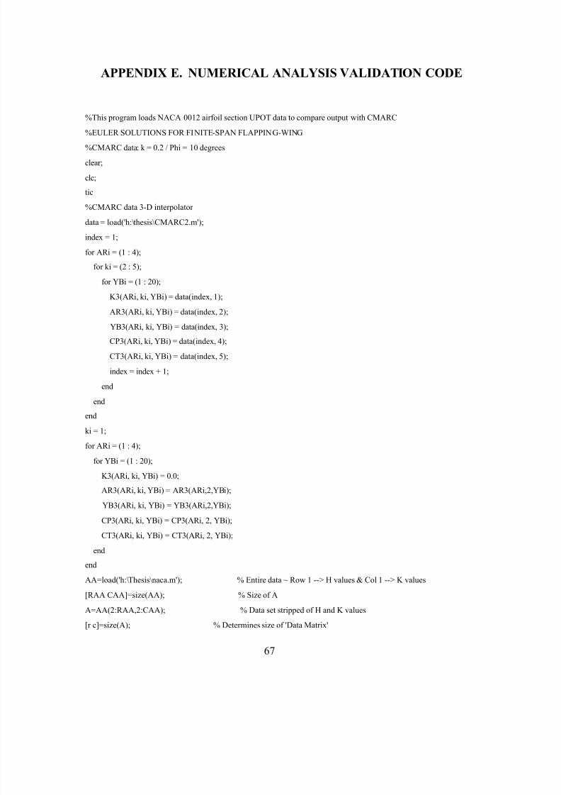
7/18/2019 02Sep Randall
http://slidepdf.com/reader/full/02sep-randall 83/112
67
APPENDIX E. NUMERICAL ANALYSIS VALIDATION CODE
%This program loads NACA 0012 airfoil section UPOT data to compare output with CMARC
%EULER SOLUTIONS FOR FINITE-SPAN FLAPPING-WING
%CMARC data: k = 0.2 / Phi = 10 degrees
clear;
clc;
tic
%CMARC data 3-D interpolator
data = load('h:\thesis\CMARC2.m');
index = 1;
for ARi = (1 : 4);
for ki = (2 : 5);
for YBi = (1 : 20);
K3(ARi, ki, YBi) = data(index, 1);
AR3(ARi, ki, YBi) = data(index, 2);
YB3(ARi, ki, YBi) = data(index, 3);
CP3(ARi, ki, YBi) = data(index, 4);
CT3(ARi, ki, YBi) = data(index, 5);
index = index + 1;
end
end
end
ki = 1;
for ARi = (1 : 4);
for YBi = (1 : 20);
K3(ARi, ki, YBi) = 0.0;
AR3(ARi, ki, YBi) = AR3(ARi,2,YBi);
YB3(ARi, ki, YBi) = YB3(ARi,2,YBi);
CP3(ARi, ki, YBi) = CP3(ARi, 2, YBi);
CT3(ARi, ki, YBi) = CT3(ARi, 2, YBi);
end
end
AA=load('h:\Thesis\naca.m'); % Entire data ~ Row 1 --> H values & Col 1 --> K values
[RAA CAA]=size(AA); % Size of A
A=AA(2:RAA,2:CAA); % Data set stripped of H and K values
[r c]=size(A); % Determines size of 'Data Matrix'
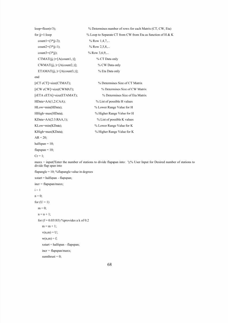
7/18/2019 02Sep Randall
http://slidepdf.com/reader/full/02sep-randall 84/112
68
loop=floor(r/3); % Determines number of rows for each Matrix (CT, CW, Eta)
for jj=1:loop % Loop to Separate CT from CW from Eta as function of H & K
count1=(3*jj-2); % Row 1,4,7,...
count2=(3*jj-1); % Row 2,5,8,...
count3=(3*jj); % Row 3,6,9,...
CTMAT(jj,:)=[A(count1,:)]; % CT Data only
CWMAT(jj,:)=[A(count2,:)]; % CW Data only
ETAMAT(jj,:)=[A(count3,:)]; % Eta Data only
end
[rCT cCT]=size(CTMAT); % Determines Size of CT Matrix
[rCW cCW]=size(CWMAT); % Determines Size of CW Matrix
[rETA cETA]=size(ETAMAT); % Determines Size of Eta Matrix
HData=AA(1,2:CAA); % List of possible H values
HLow=min(HData); % Lower Range Value for H
HHigh=max(HData); % Higher Range Value for H
KData=AA(2:3:RAA,1); % List of possible K values
KLow=min(KData); % Lower Range Value for K
KHigh=max(KData); % Higher Range Value for K
AR = 20;
halfspan = 10;
flapspan = 10;
Cr = 1;
maxx = input('Enter the number of stations to divide flapspan into: ');% User Input for Desired number of stations todivide flap span into
flapangle = 10; %flapangle value in degrees
xstart = halfspan - flapspan;
incr = flapspan/maxx;
i = 1
n = 0;
for (U = 1)
m = 0;
n = n + 1;
for (f = 0.03183) %provides a k of 0.2
m = m + 1;
v(n,m) = U;
w(n,m) = f;
xstart = halfspan - flapspan;
incr = flapspan/maxx;
sumthrust = 0;
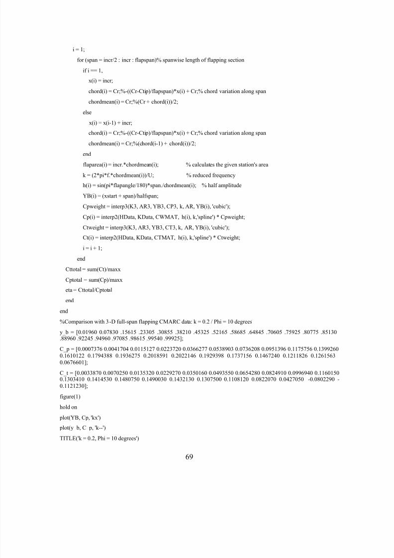
7/18/2019 02Sep Randall
http://slidepdf.com/reader/full/02sep-randall 85/112
69
i = 1;
for (span = incr/2 : incr : flapspan)% spanwise length of flapping section
if i == 1,
x(i) = incr;
chord(i) = Cr;%-((Cr-Ctip)/flapspan)*x(i) + Cr;% chord variation along span
chordmean(i) = Cr;%(Cr + chord(i))/2;
else
x(i) = x(i-1) + incr;
chord(i) = Cr;%-((Cr-Ctip)/flapspan)*x(i) + Cr;% chord variation along span
chordmean(i) = Cr;%(chord(i-1) + chord(i))/2;
end
flaparea(i) = incr.*chordmean(i); % calculates the given station's area
k = (2*pi*f.*chordmean(i))/U; % reduced frequency
h(i) = sin(pi*flapangle/180)*span./chordmean(i); % half amplitude
YB(i) = (xstart + span)/halfspan;
Cpweight = interp3(K3, AR3, YB3, CP3, k, AR, YB(i), 'cubic');
Cp(i) = interp2(HData, KData, CWMAT, h(i), k,'spline') * Cpweight;
Ctweight = interp3(K3, AR3, YB3, CT3, k, AR, YB(i), 'cubic');
Ct(i) = interp2(HData, KData, CTMAT, h(i), k,'spline') * Ctweight;
i = i + 1;
end
Cttotal = sum(Ct)/maxx
Cptotal = sum(Cp)/maxx
eta = Cttotal/Cptotal
end
end
%Comparison with 3-D full-span flapping CMARC data: k = 0.2 / Phi = 10 degrees
y_b = [0.01960 0.07830 .15615 .23305 .30855 .38210 .45325 .52165 .58685 .64845 .70605 .75925 .80775 .85130.88960 .92245 .94960 .97085 .98615 .99540 .99925];
C_p = [0.0007376 0.0041704 0.0115127 0.0223720 0.0366277 0.0538903 0.0736208 0.0951396 0.1175756 0.1399260
0.1610122 0.1794388 0.1936275 0.2018591 0.2022146 0.1929398 0.1737156 0.1467240 0.1211826 0.1261563
0.0676601];
C_t = [0.0033870 0.0070250 0.0135320 0.0229270 0.0350160 0.0493550 0.0654280 0.0824910 0.0996940 0.11601500.1303410 0.1414530 0.1480750 0.1490030 0.1432130 0.1307500 0.1108120 0.0822070 0.0427050 -0.0802290 -
0.1121230];
figure(1)
hold on
plot(YB, Cp, 'kx')
plot(y_b, C_p, 'k--')
TITLE('k = 0.2, Phi = 10 degrees')

7/18/2019 02Sep Randall
http://slidepdf.com/reader/full/02sep-randall 86/112
70
xlabel('Y/B'); ylabel('Cp')
legend('MATLAB Code','CMARC Data')
figure(2)
hold on
plot(YB, Ct, 'k:')
plot(y_b, C_t, 'k--')
TITLE('k = 0.2, Phi = 10 degrees')
xlabel('Y/B'); ylabel('Ct')
legend('MATLAB Code','CMARC Data')
toc
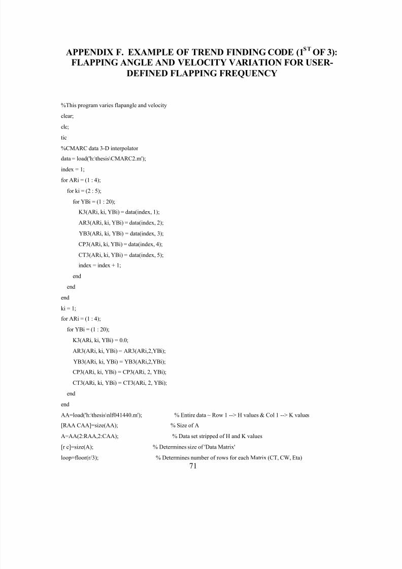
7/18/2019 02Sep Randall
http://slidepdf.com/reader/full/02sep-randall 87/112
71
APPENDIX F. EXAMPLE OF TREND FINDING CODE (1ST
OF 3):FLAPPING ANGLE AND VELOCITY VARIATION FOR USER-
DEFINED FLAPPING FREQUENCY
%This program varies flapangle and velocity
clear;
clc;
tic
%CMARC data 3-D interpolator
data = load('h:\thesis\CMARC2.m');
index = 1;
for ARi = (1 : 4);
for ki = (2 : 5);
for YBi = (1 : 20);
K3(ARi, ki, YBi) = data(index, 1);
AR3(ARi, ki, YBi) = data(index, 2);
YB3(ARi, ki, YBi) = data(index, 3);
CP3(ARi, ki, YBi) = data(index, 4);
CT3(ARi, ki, YBi) = data(index, 5);
index = index + 1;
end
end
end
ki = 1;
for ARi = (1 : 4);
for YBi = (1 : 20);
K3(ARi, ki, YBi) = 0.0;
AR3(ARi, ki, YBi) = AR3(ARi,2,YBi);
YB3(ARi, ki, YBi) = YB3(ARi,2,YBi);
CP3(ARi, ki, YBi) = CP3(ARi, 2, YBi);
CT3(ARi, ki, YBi) = CT3(ARi, 2, YBi);
end
end
AA=load('h:\thesis\nlf041440.m'); % Entire data ~ Row 1 --> H values & Col 1 --> K values
[RAA CAA]=size(AA); % Size of A
A=AA(2:RAA,2:CAA); % Data set stripped of H and K values
[r c]=size(A); % Determines size of 'Data Matrix'
loop=floor(r/3); % Determines number of rows for each Matrix (CT, CW, Eta)
7/18/2019 02Sep Randall
http://slidepdf.com/reader/full/02sep-randall 88/112
72
for jj=1:loop % Loop to Separate CT from CW from Eta as function of H & K
count1=(3*jj-2); % Row 1,4,7,...
count2=(3*jj-1); % Row 2,5,8,...
count3=(3*jj); % Row 3,6,9,...
CTMAT(jj,:)=[A(count1,:)]; % CT Data only
CWMAT(jj,:)=[A(count2,:)]; % CW Data only
ETAMAT(jj,:)=[A(count3,:)]; % Eta Data only
end
[rCT cCT]=size(CTMAT); % Determines Size of CT Matrix
[rCW cCW]=size(CWMAT); % Determines Size of CW Matrix
[rETA cETA]=size(ETAMAT); % Determines Size of Eta Matrix
HData=AA(1,2:CAA); % List of possible H values
HLow=min(HData); % Lower Range Value for H
HHigh=max(HData); % Higher Range Value for H
KData=AA(2:3:RAA,1); % List of possible K values
KLow=min(KData); % Lower Range Value for K
KHigh=max(KData); % Higher Range Value for K
rho = 1.22511; %standard s.l. density kg/m^3
flapangle = 0;
U = 0;
%the input section asks for several individual inputs and ranges for the other parameters
halfspan=input('Enter halfspan of aircraft in meters: '); % User Input for half span of aircraft
percentflap=input('Enter fraction of span that will flap '); %User input
flap_span=input('Enter 0 to apply this percentage or 1 for a full span flap: ');% User Input for Desired Flap
span
if flap_span == 0,
flapspan=percentflap*halfspan,%calculates flapspan
else flap_span == 1,
flapspan=halfspan, %the entire span flaps
end
Cr=input('Enter Cr value of flapspan in meters: ');% User Input for Desired Root Chord
Ctip=0.4*Cr; %ties Ctip to Cr via 0.4 taper ratio
AR = input('Enter the Aspect Ratio of the aircraft: '); %User input for AR
maxx=input('Enter the number of stations to divide flapspan into: ');% User Input for Desired number ofstations to divide flap span into
f=input('Enter flapping frequency in Hz: ');% User Input for flapping frequency
%Lighthawk Data
Udata = [11 11.5 12 12.5 13 13.5 14 14.5 15 15.5 16 16.5 17 17.5 18 18.5 19 19.5 20 20.5 21 21.5 22 22.5 2323.5 24 24.5 25 25.5 26 26.5 27 27.5 28 28.5 29 29.5 30 30.5 31 31.5 32];
%LightHawk Data
7/18/2019 02Sep Randall
http://slidepdf.com/reader/full/02sep-randall 89/112
73
Dragdata = [59.6497 56.6736 54.1285 51.9726 50.1565 48.6422 47.4010 46.3981 45.6205 45.0350 44.6277
44.3893 44.2897 44.3267 44.4894 44.7669 45.1509 45.6337 46.1945 46.8524 47.5867 48.3888 49.2491
50.1884 51.1642 52.2132 53.3061 54.4456 55.6352 56.8778 58.1343 59.4476 60.7981 62.1870 63.589565.0299 66.5091 67.9986 69.5256 71.0588 72.6277 74.2326 75.8370];
n = 0;
for (flapangle = .8: 0.75: 15)%5 degrees to 10 degrees in 0.5 degree increments (17)
n = n + 1;
m = 0;
for (U = 12: 0.5: 18.0)
m = m + 1;
drag = interp1(Udata, Dragdata, U,'spline');
v(n,m) = flapangle;
w(n,m) = U;
xstart = halfspan - flapspan;
incr = flapspan/maxx;
sumthrust = 0;
sumpower = 0;
i = 1;
for (span = incr/2 : incr : flapspan)% spanwise length of flapping section
if i == 1,
x(i) = incr;
chord(i) =-((Cr-Ctip)/flapspan)*x(i) + Cr;% chord variation along span
chordmean(i) = (Cr + chord(i))/2;
else
x(i) = x(i-1) + incr;
chord(i) =-((Cr-Ctip)/flapspan)*x(i) + Cr;% chord variation along span
chordmean(i) = (chord(i-1) + chord(i))/2;
end
YB = (xstart + span)/halfspan;
flaparea = incr*chordmean(i); % calculates the given station's area
k = (2*pi*f*chordmean(i))/U; % reduced frequency
h = sin(pi*flapangle/180)*span/chordmean(n); % half amplitude
Cpweight = interp3(K3, AR3, YB3, CP3, k, AR, YB, 'linear');
Cw(i) = interp2(HData, KData, CWMAT, h, k,'spline') * Cpweight;
sumpower = sumpower + Cw(i)*.5*flaparea*rho*U^3;
Ctweight = interp3(K3, AR3, YB3, CT3, k, AR, YB, 'linear');
Ct(i) = interp2(HData, KData, CTMAT, h, k,'spline') * Ctweight;
sumthrust = sumthrust + Ct(i)*.5*flaparea*rho*U^2;
i = i + 1;
end

7/18/2019 02Sep Randall
http://slidepdf.com/reader/full/02sep-randall 90/112
74
power(n,m) = 2*sumpower;
thrust(n,m) = 2*sumthrust;
eta(n,m) = (thrust(n,m)*U)/power(n,m);
netdrag(n,m) = drag - thrust(n,m); %net drag after flap thrust is subtracted
neweta(n,m) = netdrag(n,m)*U/power(n,m);
netsink(n,m) = U * netdrag(n,m)/1556.930; %net sink-rate as a function of U and drag
end
end
figure(1)
subplot(1,2,1)
surfc (v, w, thrust), xlabel('Flapangle in degrees'), ylabel('Velocity in m/s'), zlabel('Thrust in Newtons')
vec=[4,6,8,10,12,14,16,18,20,24,28,32,40,50,60,70];
subplot(1,2,2)
[ccc,hhh] = contour(v, w, thrust, vec);
xlabel('Flapangle in degrees'), ylabel('Velocity in m/s')
clabel(ccc,hhh); colorbar
figure(2)
subplot(1,2,1)
surfc (v, w, power), xlabel('Flapangle in degrees'), ylabel('Velocity in m/s'), zlabel('Power in Watts')
vec=[25,50,75,100,150,200,250,300,400,500,750,1000,1250,1500,2000,2500];
subplot(1,2,2)
[ccc,hhh] = contour(v, w, power, vec);
xlabel('Flapangle in degrees'), ylabel('Velocity in m/s')
clabel(ccc,hhh); colorbar
figure(3)
subplot(1,2,1)
surfc (v, w, eta), xlabel('Flapangle in degrees'), ylabel('Velocity in m/s'), zlabel('Efficiency')
subplot(1,2,2)
[ccc,hhh] = contour(v, w, eta);
xlabel('Flapangle in degrees'), ylabel('Velocity in m/s')
clabel(ccc,hhh); colorbar
vec=[1,2,3,4,5,10,15,20,25,30,35,40,50,75,100,150,200,250];
figure(4)
[ccc,hhh] = contour(v, w, neweta);
xlabel('Flapangle in degrees'), ylabel('Velocity in m/s')
clabel(ccc,hhh); colorbar
vec=[-0.8,-0.6,-0.4,-0.2,0,0.2,0.4,0.6];
figure(5)
[ccc,hhh] = contour(v, w, netsink, vec);

7/18/2019 02Sep Randall
http://slidepdf.com/reader/full/02sep-randall 91/112
75
xlabel('Flapangle in degrees'), ylabel('Velocity in m/s')
clabel(ccc,hhh); colorbar
toc
end

7/18/2019 02Sep Randall
http://slidepdf.com/reader/full/02sep-randall 92/112
76
THIS PAGE INTENTIONALLY LEFT BLANK
7/18/2019 02Sep Randall
http://slidepdf.com/reader/full/02sep-randall 93/112
77
APPENDIX G. CONSTRAINING CODE 1: HUMAN-POWEREDSPARROWHAWK
%This program varies velocity and frequency with a user defined maximum input power restriction
%this program calls up thrust1b.m and power1b.m functions
clear;
clc;
tic
%CMARC data 3-D interpolator
data = load('h:\thesis\CMARC2.m');
index = 1;
for ARi = (1 : 4);
for ki = (2 : 5);
for YBi = (1 : 20);
K3(ARi, ki, YBi) = data(index, 1);
AR3(ARi, ki, YBi) = data(index, 2);
YB3(ARi, ki, YBi) = data(index, 3);
CP3(ARi, ki, YBi) = data(index, 4);
CT3(ARi, ki, YBi) = data(index, 5);
index = index + 1;
end
end
end
ki = 1;
for ARi = (1 : 4);
for YBi = (1 : 20);
K3(ARi, ki, YBi) = 0.0;
AR3(ARi, ki, YBi) = AR3(ARi,2,YBi);
YB3(ARi, ki, YBi) = YB3(ARi,2,YBi);
CP3(ARi, ki, YBi) = CP3(ARi, 2, YBi);
CT3(ARi, ki, YBi) = CT3(ARi, 2, YBi);
end
end
%downloads UPOT generated data and sorts coefficients
AA=load('h:\thesis\nlf041440.m'); % Entire data ~ Row 1 --> H values & Col 1 --> K values
[RAA CAA]=size(AA); % Size of A
A=AA(2:RAA,2:CAA); % Data set stripped of H and K values
7/18/2019 02Sep Randall
http://slidepdf.com/reader/full/02sep-randall 94/112
78
[r c]=size(A); % Determines size of 'Data Matrix'
loop=floor(r/3); % Determines number of rows for each Matrix (CT, CW, Eta)
for jj=1:loop % Loop to Separate CT from CW from Eta as function of H & K
count1=(3*jj-2); % Row 1,4,7,...
count2=(3*jj-1); % Row 2,5,8,...
count3=(3*jj); % Row 3,6,9,...
CTMAT(jj,:)=[A(count1,:)]; % CT Data only
CWMAT(jj,:)=[A(count2,:)]; % CW Data only
ETAMAT(jj,:)=[A(count3,:)]; % Eta Data only
end
[rCT cCT]=size(CTMAT); % Determines Size of CT Matrix
[rCW cCW]=size(CWMAT); % Determines Size of CW Matrix
[rETA cETA]=size(ETAMAT); % Determines Size of Eta Matrix
for n=1:rCT
for m=1:cCT
if ( CTMAT(n,m) > 99 ),
CTMAT(n,m) = 0.0;
end
if ( CWMAT(n,m) > 99 ),
CWMAT(n,m) = 0.0;
end
end
end
HData=AA(1,2:CAA); % List of possible H values
HLow=min(HData); % Lower Range Value for H
HHigh=max(HData); % Higher Range Value for H
KData=AA(2:3:RAA,1); % List of possible K values
KLow=min(KData); % Lower Range Value for K
KHigh=max(KData); % Higher Range Value for K
rho = 1.22511; % standard s.l. density kg/m^3
delta = 0.001;
er = +0.005;
pi = acos(-1);
%input section asks for several individual inputs and ranges for the other parameters
AR = input('Enter the Aspect Ratio of the aircraft: '); %User input for AR
halfspan=input('Enter halfspan of aircraft in meters: ');% User Input for half span of aircraft
percentflap=input('Enter fraction of span that will flap: '); %User input span fraction
flap_span=input('Enter 0 to apply this percentage or 1 for a full span flap: ');% User Input for Desired Flapspan
7/18/2019 02Sep Randall
http://slidepdf.com/reader/full/02sep-randall 95/112
79
if flap_span == 0,
flapspan=percentflap*halfspan, %calculates flapspan
else flap_span == 1,
flapspan=halfspan, %the entire span flaps
end
Cr=input('Enter Cr value of flapspan in meters: ');% User Input for Desired Root Chord
Ctip=0.4*Cr; %ties Ctip to Cr via 0.4 taper ratio
maxx=input('Enter the number of stations to divide flapspan into: ');%Desired number of stations to divide
flapspan into
powermax=input('Enter the maximum power that is available for propulsion: ');
flapangle0=input('Enter flapangle value in degrees: ');% User Input for maximum flap angle
%SparrowHawk Data
Udata = [17.554 18.178 18.872 19.651 20.535 21.549 22.730 24.128 25.820 27.927 30.651 34.367 39.876
44.897 49.312 69.565];
%SparrowHawk Data
Dragdata = [73.874 65.914 60.094 54.778 50.070 47.678 44.806 43.100 42.817 42.617 45.232 50.346 61.130
76.650 95.302 183.925];
n = 0;
for (U = 18: 2: 34.0) %Sparrowhawk velocity range
m = 0;
n = n + 1;
flapangle = flapangle0;
drag = interp1(Udata, Dragdata, U,'spline');
for (f = 0.05: 0.05: 1.0) %Sparrowhawk frequency range
m = m + 1;
v(n,m) = U;
w(n,m) = f;
dP = 10;
%calls up function power1b
[Cw, sumpower] = power1b(flapspan, halfspan, Cr, Ctip, maxx, f, U, flapangle, HData, KData, CWMAT,
rho, K3, AR3, YB3, CP3, AR);
power(n,m) = 2*sumpower;
iter = 0;
%Iterative method for finding max thrust given limited power
if power(n,m) >= powermax,
flapangle2 = flapangle;
powern2 = power(n,m);
flapangle1 = flapangle2 - er;
while abs(dP) >= delta
7/18/2019 02Sep Randall
http://slidepdf.com/reader/full/02sep-randall 96/112
80
[Cw, sumpower] = power1b(flapspan, halfspan, Cr, Ctip, maxx, f, U, flapangle1, HData, KData,
CWMAT, rho, K3, AR3, YB3, CP3, AR);
powern1 = 2*sumpower;
flapanglen = abs(flapangle2 - (powern2 - powermax) * (flapangle2 - flapangle1)/(powern2 -
powern1));
dP = powern1 - powermax;
powern2 = powern1;
flapangle2 = flapangle1;
flapangle1 = flapanglen;
iter = iter + 1;
if iter >= 50
powern1 = 0;
flapangle1 = 0;
dP = 0
end
end
power(n,m) = powern1;
flapangle = flapangle1;
end
%calls up function thrust1b
[Ct, sumthrust] = thrust1b(flapspan, halfspan, Cr, Ctip, maxx, f, U, flapangle, HData, KData,
CTMAT, rho, K3, AR3, YB3, CT3, AR);
thrust(n,m) = 2*sumthrust;
netdrag(n,m) = drag - thrust(n,m); %net drag after flap thrust is subtracted
netsink(n,m) = U * netdrag(n,m)/1556.930; %net sink-rate as a function of U and drag
flaparray(n,m) = flapangle;
eta(n,m) = (thrust (n,m)*U)/power(n,m);
end
end
%plotting section
figure(1)
subplot(1,2,1)
surfc (v, w, netsink), xlabel('Velocity in m/s'), ylabel('f in Hz'), zlabel('netsink')
subplot(1,2,2)
vec=[.55,.555,.56,.57,.59,.61,.65,.7,.8,.9];
[ccc,hhh] = contour(v, w, netsink, vec);
xlabel('Velocity in m/s'), ylabel('f in Hz')
clabel(ccc,hhh); colorbar
figure(2)
subplot(1,2,1)
7/18/2019 02Sep Randall
http://slidepdf.com/reader/full/02sep-randall 97/112
81
surfc (v, w, netdrag), xlabel('Velocity in m/s'), ylabel('f in Hz'), zlabel('netdrag')
subplot(1,2,2)
vec=[35.5,35.75,36.25,37,38.5,40,43,47,51,55,58];
[ccc,hhh] = contour(v, w, netdrag, vec);
xlabel('Velocity in m/s'), ylabel('f in Hz')
clabel(ccc,hhh); colorbar
figure(3)
subplot(1,2,1)
surfc (v, w, thrust), xlabel('Velocity in m/s'), ylabel('f in Hz'), zlabel('Thrust in Newtons')
subplot(1,2,2)
vec=[2:1:50];
[ccc,hhh] = contour(v, w, thrust, vec);
xlabel('Velocity in m/s'), ylabel('f in Hz')
clabel(ccc,hhh); colorbar
figure(4)
subplot(1,2,1)
surfc (v, w, power), xlabel('Velocity in m/s'), ylabel('f in Hz'), zlabel('Power in Watts')
subplot(1,2,2)
vec=[10,25,50,75,100,130,160,190,199.99];
[ccc,hhh] = contour(v, w, power, vec);
xlabel('Velocity in m/s'), ylabel('f in Hz')
clabel(ccc,hhh); colorbar
figure(5)
subplot(1,2,1)
surfc (v, w, flaparray), xlabel('Velocity in m/s'), ylabel('f in Hz'), zlabel('flapangle')
subplot(1,2,2)
vec=[3:1:15];
[ccc,hhh] = contour(v, w, flaparray, vec);
xlabel('Velocity in m/s'), ylabel('f in Hz')
clabel(ccc,hhh); colorbar
figure(6)
vec=[0.76:.02:.96];
[ccc,hhh] = contour(v, w, eta, vec);
xlabel('Velocity in m/s'), ylabel('f in Hz')
clabel(ccc,hhh); colorbar
toc

7/18/2019 02Sep Randall
http://slidepdf.com/reader/full/02sep-randall 98/112
82
THIS PAGE INTENTIONALLY LEFT BLANK
7/18/2019 02Sep Randall
http://slidepdf.com/reader/full/02sep-randall 99/112
83
APPENDIX H. CONSTRAINING CODE 2: HUMAN-POWEREDLIGHT HAWK/ LIGHT HAWK-BASED SUSTAINER
%This program varies velocity and frequency with a user defined maximum input power restriction
%this program calls up thrust1b.m and power1b.m functions
clear;
clc;
tic
%CMARC data 3-D interpolator
data = load('h:\thesis\CMARC2.m');
index = 1;
for ARi = (1 : 4);
for ki = (2 : 5);
for YBi = (1 : 20);
K3(ARi, ki, YBi) = data(index, 1);
AR3(ARi, ki, YBi) = data(index, 2);
YB3(ARi, ki, YBi) = data(index, 3);
CP3(ARi, ki, YBi) = data(index, 4);
CT3(ARi, ki, YBi) = data(index, 5);
index = index + 1;
end
end
end
ki = 1;
for ARi = (1 : 4);
for YBi = (1 : 20);
K3(ARi, ki, YBi) = 0.0;
AR3(ARi, ki, YBi) = AR3(ARi,2,YBi);
YB3(ARi, ki, YBi) = YB3(ARi,2,YBi);
CP3(ARi, ki, YBi) = CP3(ARi, 2, YBi);
CT3(ARi, ki, YBi) = CT3(ARi, 2, YBi);
end
end
%downloads UPOT generated data and sorts coefficients
AA=load('h:\thesis\nlf041440.m'); % Entire data ~ Row 1 --> H values & Col 1 --> K values
[RAA CAA]=size(AA); % Size of A
A=AA(2:RAA,2:CAA); % Data set stripped of H and K values

7/18/2019 02Sep Randall
http://slidepdf.com/reader/full/02sep-randall 100/112
84
[r c]=size(A); % Determines size of 'Data Matrix'
loop=floor(r/3); % Determines number of rows for each Matrix (CT, CW, Eta)
for jj=1:loop % Loop to Separate CT from CW from Eta as function of H & K
count1=(3*jj-2); % Row 1,4,7,...
count2=(3*jj-1); % Row 2,5,8,...
count3=(3*jj); % Row 3,6,9,...
CTMAT(jj,:)=[A(count1,:)]; % CT Data only
CWMAT(jj,:)=[A(count2,:)]; % CW Data only
ETAMAT(jj,:)=[A(count3,:)]; % Eta Data only
end
[rCT cCT]=size(CTMAT); % Determines Size of CT Matrix
[rCW cCW]=size(CWMAT); % Determines Size of CW Matrix
[rETA cETA]=size(ETAMAT); % Determines Size of Eta Matrix
for n=1:rCT
for m=1:cCT
if ( CTMAT(n,m) > 99 ),
CTMAT(n,m) = 0.0;
end
if ( CWMAT(n,m) > 99 ),
CWMAT(n,m) = 0.0;
end
end
end
HData=AA(1,2:CAA); % List of possible H values
HLow=min(HData); % Lower Range Value for H
HHigh=max(HData); % Higher Range Value for H
KData=AA(2:3:RAA,1); % List of possible K values
KLow=min(KData); % Lower Range Value for K
KHigh=max(KData); % Higher Range Value for K
rho = 1.22511; % standard s.l. density kg/m^3
delta = 0.001;
er = +0.005;
pi = acos(-1);
%input section asks for several individual inputs and ranges for the other parameters
AR = input('Enter the Aspect Ratio of the aircraft: '); %User input for AR
halfspan=input('Enter halfspan of aircraft in meters: ');% User Input for half span of aircraft
percentflap=input('Enter fraction of span that will flap: '); %User input span fraction
flap_span=input('Enter 0 to apply this percentage or 1 for a full span flap: ');% User Input for Desired Flapspan
7/18/2019 02Sep Randall
http://slidepdf.com/reader/full/02sep-randall 101/112
85
if flap_span == 0,
flapspan=percentflap*halfspan, %calculates flapspan
else flap_span == 1,
flapspan=halfspan, %the entire span flaps
end
Cr=input('Enter Cr value of flapspan in meters: ');% User Input for Desired Root Chord
Ctip=0.4*Cr; %ties Ctip to Cr via 0.4 taper ratio
maxx=input('Enter the number of stations to divide flapspan into: ');%Desired number of stations to divide
flapspan into
powermax=input('Enter the maximum power that is available for propulsion: ');
flapangle0=input('Enter flapangle value in degrees: ');% User Input for maximum flap angle
%LightHawk Data
Udata = [11 11.5 12 12.5 13 13.5 14 14.5 15 15.5 16 16.5 17 17.5 18 18.5 19 19.5 20 20.5 21 21.5 22 22.5 23
23.5 24 24.5 25 25.5 26 26.5 27 27.5 28 28.5 29 29.5 30 30.5 31 31.5 32];
%LightHawk Data
Dragdata = [59.6497 56.6736 54.1285 51.9726 50.1565 48.6422 47.4010 46.3981 45.6205 45.0350 44.6277
44.3893 44.2897 44.3267 44.4894 44.7669 45.1509 45.6337 46.1945 46.8524 47.5867 48.3888 49.249150.1884 51.1642 52.2132 53.3061 54.4456 55.6352 56.8778 58.1343 59.4476 60.7981 62.1870 63.5895
65.0299 66.5091 67.9986 69.5256 71.0588 72.6277 74.2326 75.8370];
n = 0;
for (U = 11.5: 2: 26.0) %Lighthawk velocity range
m = 0;
n = n + 1;
flapangle = flapangle0;
drag = interp1(Udata, Dragdata, U,'spline');
for (f = 0.05: 0.05: 0.7) %Lighthawk frequency range
m = m + 1;
v(n,m) = U;
w(n,m) = f;
dP = 10;
%calls up function power1b
[Cw, sumpower] = power1b(flapspan, halfspan, Cr, Ctip, maxx, f, U, flapangle, HData, KData, CWMAT,rho, K3, AR3, YB3, CP3, AR);
power(n,m) = 2*sumpower;
iter = 0;
%Iterative method for finding max thrust given limited power
if power(n,m) >= powermax,
flapangle2 = flapangle;
powern2 = power(n,m);
flapangle1 = flapangle2 - er;
7/18/2019 02Sep Randall
http://slidepdf.com/reader/full/02sep-randall 102/112
86
while abs(dP) >= delta
[Cw, sumpower] = power1b(flapspan, halfspan, Cr, Ctip, maxx, f, U, flapangle1, HData, KData,
CWMAT, rho, K3, AR3, YB3, CP3, AR);
powern1 = 2*sumpower;
flapanglen = abs(flapangle2 - (powern2 - powermax) * (flapangle2 - flapangle1)/(powern2 -
powern1));
dP = powern1 - powermax;
powern2 = powern1;
flapangle2 = flapangle1;
flapangle1 = flapanglen;
iter = iter + 1;
if iter >= 50
powern1 = 0;
flapangle1 = 0;
dP = 0;
end
end
power(n,m) = powern1;
flapangle = flapangle1;
end
%calls up function thrust1b
[Ct, sumthrust] = thrust1b(flapspan, halfspan, Cr, Ctip, maxx, f, U, flapangle, HData, KData,
CTMAT, rho, K3, AR3, YB3, CT3, AR);
thrust(n,m) = 2*sumthrust;
netdrag(n,m) = drag - thrust(n,m); %net drag after flap thrust is subtracted
netsink(n,m) = U * netdrag(n,m)/1556.930; %net sink-rate as a function of U and drag
flaparray(n,m) = flapangle;
eta(n,m) = (thrust(n,m)*U)/power(n,m);
end
end
%plotting section
figure(1)
subplot(1,2,1)
surfc (v, w, netsink), xlabel('Velocity in m/s'), ylabel('f in Hz'), zlabel('netsink')
subplot(1,2,2)
vec=[.31,.32,.34,.36,.40,.44,.48,.52,.58,.64,.70,.78,.84];
[ccc,hhh] = contour(v, w, netsink, vec);
xlabel('Velocity in m/s'), ylabel('f in Hz')
clabel(ccc,hhh); colorbar
figure(2)

7/18/2019 02Sep Randall
http://slidepdf.com/reader/full/02sep-randall 103/112
87
subplot(1,2,1)
surfc (v, w, netdrag), xlabel('Velocity in m/s'), ylabel('f in Hz'), zlabel('netdrag')
subplot(1,2,2)
vec=[34:34.25:34.50,35.5,36.5,38,40,42,44,46,48,50];
[ccc,hhh] = contour(v, w, netdrag, vec);
xlabel('Velocity in m/s'), ylabel('f in Hz')
clabel(ccc,hhh); colorbar
figure(3)
subplot(1,2,1)
surfc (v, w, thrust), xlabel('Velocity in m/s'), ylabel('f in Hz'), zlabel('Thrust in Newtons')
subplot(1,2,2)
vec=[2:1:50];
[ccc,hhh] = contour(v, w, thrust, vec);
xlabel('Velocity in m/s'), ylabel('f in Hz')
clabel(ccc,hhh); colorbar
figure(4)
subplot(1,2,1)
surfc (v, w, power), xlabel('Velocity in m/s'), ylabel('f in Hz'), zlabel('Power in Watts')
subplot(1,2,2)
vec=[10,25,50,75,100,130,160,190,199.99];
[ccc,hhh] = contour(v, w, power, vec);
xlabel('Velocity in m/s'), ylabel('f in Hz')
clabel(ccc,hhh); colorbar
figure(5)
subplot(1,2,1)
surfc (v, w, flaparray), xlabel('Velocity in m/s'), ylabel('f in Hz'), zlabel('flapangle')
subplot(1,2,2)
vec=[2.5:.5:10];
[ccc,hhh] = contour(v, w, flaparray, vec);
xlabel('Velocity in m/s'), ylabel('f in Hz')
clabel(ccc,hhh); colorbar
figure(6)
vec=[0.74:.02:.96];
[ccc,hhh] = contour(v, w, eta, vec);
xlabel('Velocity in m/s'), ylabel('f in Hz')
clabel(ccc,hhh); colorbar
figure(7)
subplot(1,2,1)
surfc (v, w, flaparray), xlabel('Velocity in m/s'), ylabel('f in Hz'), zlabel('flapangle')

7/18/2019 02Sep Randall
http://slidepdf.com/reader/full/02sep-randall 104/112
88
subplot(1,2,2)
surfc (v, w, power), xlabel('Velocity in m/s'), ylabel('f in Hz'), zlabel('Power in Watts')
toc

7/18/2019 02Sep Randall
http://slidepdf.com/reader/full/02sep-randall 105/112
89
APPENDIX I. POWER FUNCTION CALLED BY CONSTRAININGCODES
%this function is a requirement for the restrictimizeB.m program
function [Cw, sumpower] = power1b(flapspan, halfspan, Cr, Ctip, maxx, f, U, flapangle, HData,
KData, CWMAT, rho, K3, AR3, YB3, CP3, AR);
xstart = halfspan - flapspan;
incr = flapspan/maxx;
sumpower = 0;
n = 1;
for (span = incr/2 : incr : flapspan)% spanwise length of flapping section
if n == 1,
x(n) = incr;
chord(n) =-((Cr-Ctip)/flapspan)*x(n) + Cr;% chord variation along span
chordmean(n) = (Cr + chord(n))/2;
else
x(n) = x(n-1) + incr;
chord(n) =-((Cr-Ctip)/flapspan)*x(n) + Cr;% chord variation along span
chordmean(n) = (chord(n-1) + chord(n))/2;
end
YB = (xstart + span)/halfspan;
flaparea = incr*chordmean(n); % calculates the given station's areak = (2*pi*f*chordmean(n))/U; % reduced frequency
h = sin(pi*flapangle/180)*span/chordmean(n); % half amplitude
Cpweight = interp3(K3, AR3, YB3, CP3, k, AR, YB, 'linear');
Cw(n) = interp2(HData, KData, CWMAT, h, k,'spline') * Cpweight;
sumpower = sumpower + Cw(n)*.5*flaparea*rho*U^3;
n = n + 1;
end

7/18/2019 02Sep Randall
http://slidepdf.com/reader/full/02sep-randall 106/112
90
THIS PAGE INTENTIONALLY LEFT BLANK
7/18/2019 02Sep Randall
http://slidepdf.com/reader/full/02sep-randall 107/112
91
APPENDIX J. THRUST FUNCTION CALLED BY CONSTRAININGCODES
%this function is a requirement for the restrictimizeB.m program
function [Ct, sumthrust] = thrust1b(flapspan, halfspan, Cr, Ctip, maxx, f, U, flapangle, HData,
KData, CTMAT, rho, K3, AR3, YB3, CT3, AR);
xstart = halfspan - flapspan;
incr = flapspan/maxx;
sumthrust = 0;
n = 1;
for (span = incr/2 : incr : flapspan)% spanwise length of flapping section
if n == 1,
x(n) = incr;
chord(n) =-((Cr-Ctip)/flapspan)*x(n) + Cr;% chord variation along span
chordmean(n) = (Cr + chord(n))/2;
else
x(n) = x(n-1) + incr;
chord(n) =-((Cr-Ctip)/flapspan)*x(n) + Cr;% chord variation along span
chordmean(n) = (chord(n-1) + chord(n))/2;
end
YB = (xstart + span)/halfspan;
flaparea = incr*chordmean(n); % calculates the given station's areak = (2*pi*f*chordmean(n))/U; % reduced frequency
h = sin(pi*flapangle/180)*span/chordmean(n); % half amplitude
Ctweight = interp3(K3, AR3, YB3, CT3, k, AR, YB, 'linear');
Ct(n) = interp2(HData, KData, CTMAT, h, k,'spline') * Ctweight;
sumthrust = sumthrust + Ct(n)*.5*flaparea*rho*U^2;
n = n + 1;
end

7/18/2019 02Sep Randall
http://slidepdf.com/reader/full/02sep-randall 108/112
92
THIS PAGE INTENTIONALLY LEFT BLANK
7/18/2019 02Sep Randall
http://slidepdf.com/reader/full/02sep-randall 109/112
93
LIST OF REFERENCES
1. Teng, N. H., “The Development of a Computer Code for the Numerical Solution
of Unsteady, Inviscid and Incompressible Flow over an Airfoil,” Master’s Thesis,
Naval Postgraduate School, Monterey, California, June 1987.
2. Knoller, R., “Die Gesetz des Luftwiderstandes,” Flug- und Motortechnik (Wien),Vol. 3, No. 21, 1909, pp. 1-7.
3. Betz, A., “Ein Beitrag zur Erklarung des Segelfluges,” Zeitschrift fur Flugtechnik
und Motorluftschiffahrt, Vol. 3, Jan. 1912, pp. 269-272.
4. Jones, K.D., Lund, T.C., Platzer, M.F., “Experimental and Computational
Investigation of Flapping-Wing Propulsion for Micro-Air Vehicles,” Chapter 16,AIAA Fixed and Flapping-wing Aerodynamics for Micro Air Vehicle
Applications, Ed. T. Mueller, AIAA, Reston, VA, 2001, pp. 307-339.
5. Pendaries, C., Boiffier, J.L., Jeanneau, M., “Flexible Aircraft in Conceptual
Design HALEs on the Way to Ornithopter,” AIAA Paper no. 98-0505, Reno, Nevada, January 1998.
6. Schultz, S., Princeton Weekly Bulletin, Vol. 89, No. 8, November 8, 1999.
7. McMasters, J., “The Optimization of Man-Powered Aircraft,” AIAA Paper No.71-798, School of Aeronautics, Astronautics and Engineering Sciences Purdue
University, 1971.
8. Correspondence with G. Cole, of Windward Performance LLC, www.windward-
performance.com, February-September 2002.
9. Correspondence with D. Howell, of Glidersport, www.glidersport.net, February-September 2002.
10. Spicer, J.B., associate professor Johns Hopkins University, Johns HopkinsMagazine, November 1999.)
11. Alexander, R.M., “Springs for Wings,” Science, Vol. 268, Presssssssss, 07 April
1995, pp. 50-51.
12. Jones, K.D., Castro, B.M., Mahmoud, O., Pollard, S.J. and Platzer, M. F., “A
Collaborative Numerical and Experimental Investigation of Flapping-WingPropulsion,” AIAA Paper No. 2002-0706, Reno, Nevada, January 2002.
7/18/2019 02Sep Randall
http://slidepdf.com/reader/full/02sep-randall 110/112
94
13. Hess, J.L. and Smith, A.M.O., “Calculation of Potential Flow About ArbitraryBodies,” Progress in Aeronautical Sciences, Vol. 8, Pergamon Press, Oxford,
1966, pp. 1-138.
14. Basu, B. C. and Hancock, G. J., “The Unsteady Motion of a Two-Dimensional
Aerofoil in Incompressible Inviscid Flow,” Journal of Fluid Mechanics, Vol. 87,1978, pp. 159-168.
15. Jones, K.D., Center, K.B., “Numerical Wake Visualization for Airfoils
Undergoing Forced and Aeroelastic Motions,” AIAA Paper No. 96-0055, Reno, Nevada, January 1996.
16. Jones, K.D. and Platzer, M. F., “An Experimental and Numerical Investigation ofFlapping-Wing Propulsion,” AIAA Paper No. 99-0995, Reno, Nevada, January
1999.
17. Jones, K.D., Castro, B.M., Mahmoud, O. and Platzer, M. F., “A Numerical andExperimental Investigation of Flapping-Wing Propulsion in Ground Effect,”AIAA Paper No. 2002-0866, Reno, Nevada, January 2002.
18. Jones, K.D. and Platzer, M. F., “Numerical Computation of Flapping-Wing
Propulsion and Power Extraction,” AIAA Paper No. 97-0826, Reno, Nevada,January 1997.
19. Jones, K.D., Dohring, C.M., and Platzer, M. F., “Experimental and Computational
Investigation of the Knoller-Betz Effect,” AIAA Journal 36, 1998 pp.1240-1246
20. Radaspiel, R.; Rossow, C. and Swanson, R.C.: Efficient Cell Vertex MultigridScheme for the Three-Dimensional Navier-Stokes Equations. AIAA Journal 28,
1990, pp. 1464-1472.
21. Kroll, N.; Radaspiel, R. and Rossow, C.: Accurate and Efficient Flow Solvers for3-D Applications on Structural Meshes. In: VKI Lecture Series 1994-04,“Computational Fluid Dynamics,” Brussels, 1994.
22. Rossow, C.; Kroll, N.; Radaspiel, R. and Scherr, S.: Investigation of the Accuracy
of Finite Volume Methods for 2- and 3-Dimensional Flow. In: Validation ofComputational Fluid Dynamics, AGARD CP-437, Vol. II, 1988, pp. P14-1 toP14-11.
23. Correspondence with S. Pollard, Naval Postgraduate School, July-August 2002.
7/18/2019 02Sep Randall
http://slidepdf.com/reader/full/02sep-randall 111/112
95
INITIAL DISTRIBUTION LIST
1. Defense Technical Information Center
Ft. Belvoir, VA
2. Dudley Knox Library Naval Postgraduate SchoolMonterey, CA
3. Prof. Max Platzer
Department of Aeronautics and Astronautics Naval Postgraduate SchoolMonterey, CA
4. Dr. Kevin D. Jones, Code AA/Jo
Department of Aeronautics and Astronautics Naval Postgraduate SchoolMonterey, CA
5. Steve Pollard
Naval Postgraduate SchoolMonterey, CA
6. Albion H. BowersDryden Flight Research Center
Mail Stop D2027
P.O. Box 273Edwards, CA

7/18/2019 02Sep Randall
http://slidepdf.com/reader/full/02sep-randall 112/112
THIS PAGE INTENTIONALLY LEFT BLANK