03 probability review for analysis of algorithms
TRANSCRIPT
Analysis of AlgorithmsProbability Review
Andres Mendez-Vazquez
August 31, 2015
1 / 57
Outline
1 Basic TheoryIntuitive FormulationAxiomsUnconditional and Conditional ProbabilityPosterior (Conditional) Probability
2 Random VariablesTypes of Random VariablesCumulative Distributive FunctionProperties of the PMF/PDFExpected Value and Variance
2 / 57
Outline
1 Basic TheoryIntuitive FormulationAxiomsUnconditional and Conditional ProbabilityPosterior (Conditional) Probability
2 Random VariablesTypes of Random VariablesCumulative Distributive FunctionProperties of the PMF/PDFExpected Value and Variance
3 / 57
Gerolamo Cardano: Gambling out of Darkness
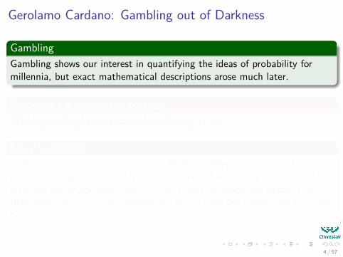
GamblingGambling shows our interest in quantifying the ideas of probability formillennia, but exact mathematical descriptions arose much later.
Gerolamo Cardano (16th century)While gambling he developed the following rule!!!
Equal conditions“The most fundamental principle of all in gambling is simply equalconditions, e.g. of opponents, of bystanders, of money, of situation, of thedice box and of the dice itself. To the extent to which you depart fromthat equity, if it is in your opponent’s favour, you are a fool, and if in yourown, you are unjust.”
4 / 57

Gerolamo Cardano: Gambling out of Darkness
GamblingGambling shows our interest in quantifying the ideas of probability formillennia, but exact mathematical descriptions arose much later.
Gerolamo Cardano (16th century)While gambling he developed the following rule!!!
Equal conditions“The most fundamental principle of all in gambling is simply equalconditions, e.g. of opponents, of bystanders, of money, of situation, of thedice box and of the dice itself. To the extent to which you depart fromthat equity, if it is in your opponent’s favour, you are a fool, and if in yourown, you are unjust.”
4 / 57

Gerolamo Cardano’s Definition
Probability“If therefore, someone should say, I want an ace, a deuce, or a trey, youknow that there are 27 favourable throws, and since the circuit is 36, therest of the throws in which these points will not turn up will be 9; theodds will therefore be 3 to 1.”
MeaningProbability as a ratio of favorable to all possible outcomes!!! As long allevents are equiprobable...
Thus, we get
P(All favourable throws) = Number All favourable throwsNumber of All throws (1)
5 / 57

Intuitive Formulation
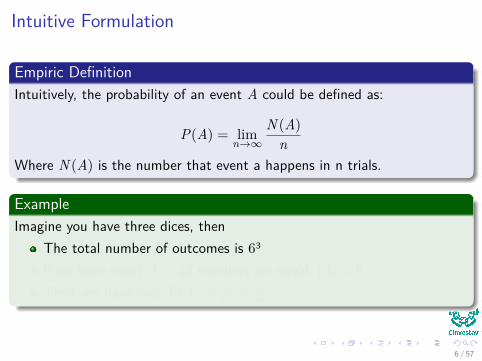
Empiric DefinitionIntuitively, the probability of an event A could be defined as:
P(A) = limn→∞
N (A)n
Where N (A) is the number that event a happens in n trials.
ExampleImagine you have three dices, then
The total number of outcomes is 63If we have event A = all numbers are equal, |A| = 6Then, we have that P(A) = 6
63 = 136
6 / 57
Intuitive Formulation
Empiric DefinitionIntuitively, the probability of an event A could be defined as:
P(A) = limn→∞
N (A)n
Where N (A) is the number that event a happens in n trials.
ExampleImagine you have three dices, then
The total number of outcomes is 63If we have event A = all numbers are equal, |A| = 6Then, we have that P(A) = 6
63 = 136
6 / 57

Outline
1 Basic TheoryIntuitive FormulationAxiomsUnconditional and Conditional ProbabilityPosterior (Conditional) Probability
2 Random VariablesTypes of Random VariablesCumulative Distributive FunctionProperties of the PMF/PDFExpected Value and Variance
7 / 57
Axioms of Probability
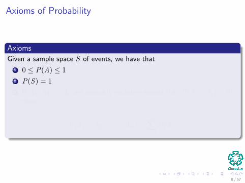
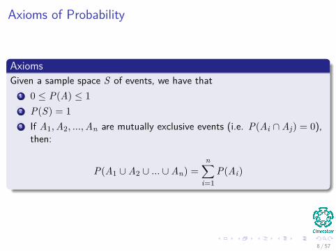
AxiomsGiven a sample space S of events, we have that
1 0 ≤ P(A) ≤ 12 P(S) = 13 If A1,A2, ...,An are mutually exclusive events (i.e. P(Ai ∩Aj) = 0),
then:
P(A1 ∪A2 ∪ ... ∪An) =n∑
i=1P(Ai)
8 / 57

Axioms of Probability
AxiomsGiven a sample space S of events, we have that
1 0 ≤ P(A) ≤ 12 P(S) = 13 If A1,A2, ...,An are mutually exclusive events (i.e. P(Ai ∩Aj) = 0),
then:
P(A1 ∪A2 ∪ ... ∪An) =n∑
i=1P(Ai)
8 / 57
Axioms of Probability
AxiomsGiven a sample space S of events, we have that
1 0 ≤ P(A) ≤ 12 P(S) = 13 If A1,A2, ...,An are mutually exclusive events (i.e. P(Ai ∩Aj) = 0),
then:
P(A1 ∪A2 ∪ ... ∪An) =n∑
i=1P(Ai)
8 / 57
Axioms of Probability
AxiomsGiven a sample space S of events, we have that
1 0 ≤ P(A) ≤ 12 P(S) = 13 If A1,A2, ...,An are mutually exclusive events (i.e. P(Ai ∩Aj) = 0),
then:
P(A1 ∪A2 ∪ ... ∪An) =n∑
i=1P(Ai)
8 / 57

Set Operations
We are usingSet Notation
ThusWhat Operations?
9 / 57

Set Operations
We are usingSet Notation
ThusWhat Operations?
9 / 57

Example
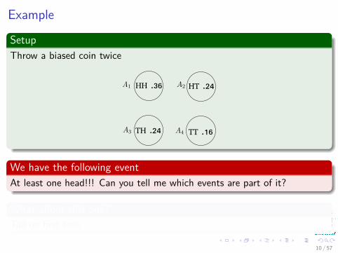
SetupThrow a biased coin twice
HH .36 HT .24
TH .24 TT .16
We have the following eventAt least one head!!! Can you tell me which events are part of it?
What about this one?Tail on first toss.
10 / 57
Example
SetupThrow a biased coin twice
HH .36 HT .24
TH .24 TT .16
We have the following eventAt least one head!!! Can you tell me which events are part of it?
What about this one?Tail on first toss.
10 / 57

Example
SetupThrow a biased coin twice
HH .36 HT .24
TH .24 TT .16
We have the following eventAt least one head!!! Can you tell me which events are part of it?
What about this one?Tail on first toss.
10 / 57
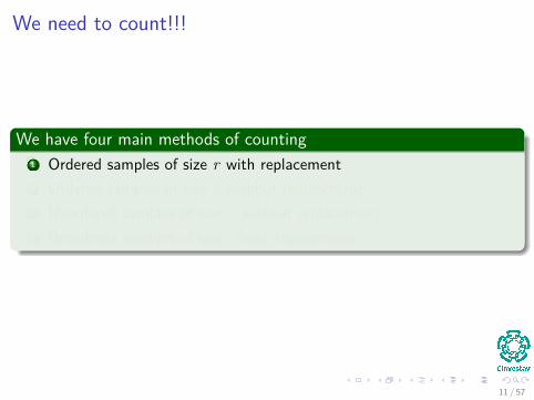
We need to count!!!
We have four main methods of counting1 Ordered samples of size r with replacement2 Ordered samples of size r without replacement3 Unordered samples of size r without replacement4 Unordered samples of size r with replacement
11 / 57

We need to count!!!
We have four main methods of counting1 Ordered samples of size r with replacement2 Ordered samples of size r without replacement3 Unordered samples of size r without replacement4 Unordered samples of size r with replacement
11 / 57

We need to count!!!
We have four main methods of counting1 Ordered samples of size r with replacement2 Ordered samples of size r without replacement3 Unordered samples of size r without replacement4 Unordered samples of size r with replacement
11 / 57

We need to count!!!
We have four main methods of counting1 Ordered samples of size r with replacement2 Ordered samples of size r without replacement3 Unordered samples of size r without replacement4 Unordered samples of size r with replacement
11 / 57

Ordered samples of size r with replacement
DefinitionThe number of possible sequences (ai1 , ..., air ) for n different numbers isn × n × ...× n = nr
ExampleIf you throw three dices you have 6× 6× 6 = 216
12 / 57

Ordered samples of size r with replacement
DefinitionThe number of possible sequences (ai1 , ..., air ) for n different numbers isn × n × ...× n = nr
ExampleIf you throw three dices you have 6× 6× 6 = 216
12 / 57

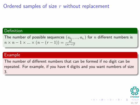
Ordered samples of size r without replacement
DefinitionThe number of possible sequences (ai1 , ..., air ) for n different numbers isn × n − 1× ...× (n − (r − 1)) = n!
(n−r)!
ExampleThe number of different numbers that can be formed if no digit can berepeated. For example, if you have 4 digits and you want numbers of size3.
13 / 57
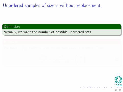
Unordered samples of size r without replacement
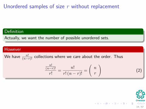
DefinitionActually, we want the number of possible unordered sets.
HoweverWe have n!
(n−r)! collections where we care about the order. Thus
n!(n−r)!
r ! = n!r ! (n − r)! =
(nr
)(2)
14 / 57
Unordered samples of size r without replacement
DefinitionActually, we want the number of possible unordered sets.
HoweverWe have n!
(n−r)! collections where we care about the order. Thus
n!(n−r)!
r ! = n!r ! (n − r)! =
(nr
)(2)
14 / 57
Unordered samples of size r with replacement
DefinitionWe want to find an unordered set ai1 , ..., air with replacement
Thus (n + r − 1
r
)(3)
15 / 57

Unordered samples of size r with replacement
DefinitionWe want to find an unordered set ai1 , ..., air with replacement
Thus (n + r − 1
r
)(3)
15 / 57
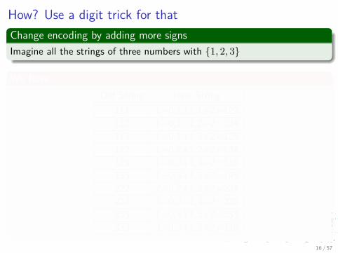
How? Use a digit trick for thatChange encoding by adding more signsImagine all the strings of three numbers with 1, 2, 3
We haveOld String New String
111 1+0,1+1,1+2=123112 1+0,1+1,2+2=124113 1+0,1+1,3+2=125122 1+0,2+1,2+2=134123 1+0,2+1,3+2=135133 1+0,3+1,3+2=145222 2+0,2+1,2+2=234223 2+0,2+1,3+2=225233 1+0,3+1,3+2=233333 3+0,3+1,3+2=345
16 / 57
Independence
DefinitionTwo events A and B are independent if and only ifP(A,B) = P(A ∩ B) = P(A)P(B)
17 / 57
Example
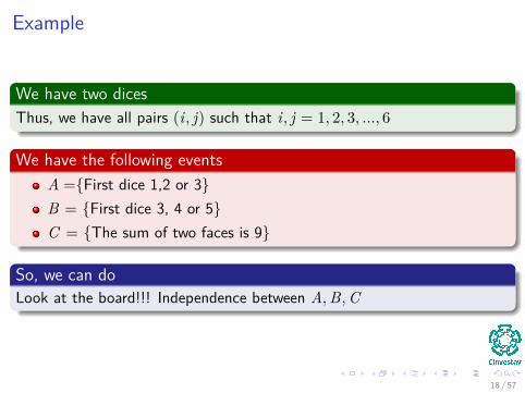
We have two dicesThus, we have all pairs (i, j) such that i, j = 1, 2, 3, ..., 6
We have the following eventsA =First dice 1,2 or 3B = First dice 3, 4 or 5C = The sum of two faces is 9
So, we can doLook at the board!!! Independence between A,B,C
18 / 57

Example
We have two dicesThus, we have all pairs (i, j) such that i, j = 1, 2, 3, ..., 6
We have the following eventsA =First dice 1,2 or 3B = First dice 3, 4 or 5C = The sum of two faces is 9
So, we can doLook at the board!!! Independence between A,B,C
18 / 57

Example
We have two dicesThus, we have all pairs (i, j) such that i, j = 1, 2, 3, ..., 6
We have the following eventsA =First dice 1,2 or 3B = First dice 3, 4 or 5C = The sum of two faces is 9
So, we can doLook at the board!!! Independence between A,B,C
18 / 57

Example
We have two dicesThus, we have all pairs (i, j) such that i, j = 1, 2, 3, ..., 6
We have the following eventsA =First dice 1,2 or 3B = First dice 3, 4 or 5C = The sum of two faces is 9
So, we can doLook at the board!!! Independence between A,B,C
18 / 57
Example
We have two dicesThus, we have all pairs (i, j) such that i, j = 1, 2, 3, ..., 6
We have the following eventsA =First dice 1,2 or 3B = First dice 3, 4 or 5C = The sum of two faces is 9
So, we can doLook at the board!!! Independence between A,B,C
18 / 57
We can use to derive the Binomial Distribution
WHAT?????
19 / 57
First, we use a sequence of n Bernoulli Trials
We have this“Success” has a probability p.“Failure” has a probability 1− p.
ExamplesToss a coin independently n times.Examine components produced on an assembly line.
NowWe take S =all 2n ordered sequences of length n, with components0(failure) and 1(success).
20 / 57
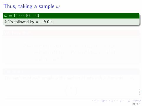
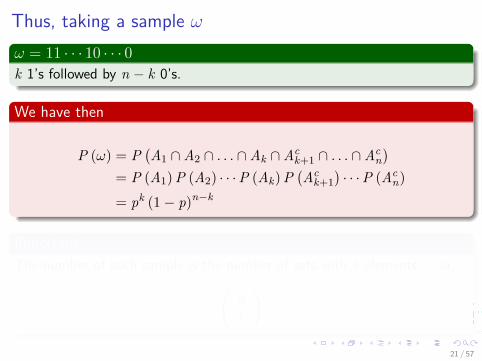
Thus, taking a sample ω
ω = 11 · · · 10 · · · 0k 1’s followed by n − k 0’s.
We have then
P (ω) = P(A1 ∩A2 ∩ . . . ∩Ak ∩Ac
k+1 ∩ . . . ∩Acn)
= P (A1) P (A2) · · ·P (Ak) P(Ac
k+1)· · ·P (Ac
n)= pk (1− p)n−k
ImportantThe number of such sample is the number of sets with k elements.... or...(
nk
)
21 / 57

Did you notice?
We do not care where the 1’s and 0’s areThus all the probabilities are equal to pk (1− p)k
Thus, we are looking to sum all those probabilities of all thosecombinations of 1’s and 0’s ∑
k 1’sp(ωk)
Then ∑k 1’s
p(ωk)
=(
nk
)p (1− p)n−k
22 / 57

Did you notice?
We do not care where the 1’s and 0’s areThus all the probabilities are equal to pk (1− p)k
Thus, we are looking to sum all those probabilities of all thosecombinations of 1’s and 0’s ∑
k 1’sp(ωk)
Then ∑k 1’s
p(ωk)
=(
nk
)p (1− p)n−k
22 / 57

Did you notice?
We do not care where the 1’s and 0’s areThus all the probabilities are equal to pk (1− p)k
Thus, we are looking to sum all those probabilities of all thosecombinations of 1’s and 0’s ∑
k 1’sp(ωk)
Then ∑k 1’s
p(ωk)
=(
nk
)p (1− p)n−k
22 / 57
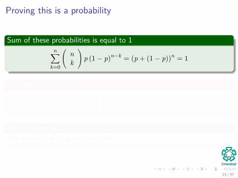
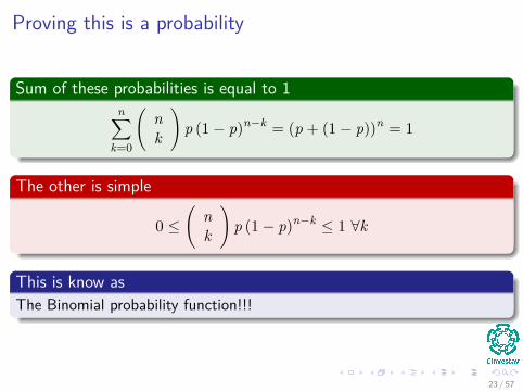
Proving this is a probability
Sum of these probabilities is equal to 1n∑
k=0
(nk
)p (1− p)n−k = (p + (1− p))n = 1
The other is simple
0 ≤(
nk
)p (1− p)n−k ≤ 1 ∀k
This is know asThe Binomial probability function!!!
23 / 57

Proving this is a probability
Sum of these probabilities is equal to 1n∑
k=0
(nk
)p (1− p)n−k = (p + (1− p))n = 1
The other is simple
0 ≤(
nk
)p (1− p)n−k ≤ 1 ∀k
This is know asThe Binomial probability function!!!
23 / 57
Proving this is a probability
Sum of these probabilities is equal to 1n∑
k=0
(nk
)p (1− p)n−k = (p + (1− p))n = 1
The other is simple
0 ≤(
nk
)p (1− p)n−k ≤ 1 ∀k
This is know asThe Binomial probability function!!!
23 / 57
Outline
1 Basic TheoryIntuitive FormulationAxiomsUnconditional and Conditional ProbabilityPosterior (Conditional) Probability
2 Random VariablesTypes of Random VariablesCumulative Distributive FunctionProperties of the PMF/PDFExpected Value and Variance
24 / 57

Different Probabilities
UnconditionalThis is the probability of an event A prior to arrival of any evidence, it isdenoted by P(A). For example:
P(Cavity)=0.1 means that “in the absence of any other information,there is a 10% chance that the patient is having a cavity”.
ConditionalThis is the probability of an event A given some evidence B, it is denotedP(A|B). For example:
P(Cavity/Toothache)=0.8 means that “there is an 80% chance thatthe patient is having a cavity given that he is having a toothache”
25 / 57

Outline
1 Basic TheoryIntuitive FormulationAxiomsUnconditional and Conditional ProbabilityPosterior (Conditional) Probability
2 Random VariablesTypes of Random VariablesCumulative Distributive FunctionProperties of the PMF/PDFExpected Value and Variance
26 / 57

Posterior Probabilities
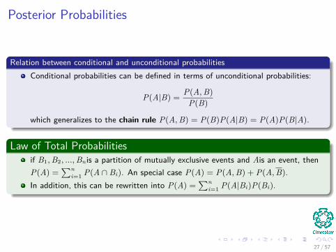
Relation between conditional and unconditional probabilitiesConditional probabilities can be defined in terms of unconditional probabilities:
P(A|B) = P(A, B)P(B)
which generalizes to the chain rule P(A, B) = P(B)P(A|B) = P(A)P(B|A).
Law of Total Probabilitiesif B1, B2, ..., Bn is a partition of mutually exclusive events and Ais an event, thenP(A) =
∑ni=1 P(A ∩ Bi). An special case P(A) = P(A, B) + P(A, B).
In addition, this can be rewritten into P(A) =∑n
i=1 P(A|Bi)P(Bi).
27 / 57
Posterior Probabilities
Relation between conditional and unconditional probabilitiesConditional probabilities can be defined in terms of unconditional probabilities:
P(A|B) = P(A, B)P(B)
which generalizes to the chain rule P(A, B) = P(B)P(A|B) = P(A)P(B|A).
Law of Total Probabilitiesif B1, B2, ..., Bn is a partition of mutually exclusive events and Ais an event, thenP(A) =
∑ni=1 P(A ∩ Bi). An special case P(A) = P(A, B) + P(A, B).
In addition, this can be rewritten into P(A) =∑n
i=1 P(A|Bi)P(Bi).
27 / 57
Example
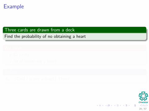
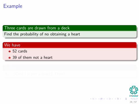
Three cards are drawn from a deckFind the probability of no obtaining a heart
We have52 cards39 of them not a heart
DefineAi =Card i is not a heart Then?
28 / 57
Example
Three cards are drawn from a deckFind the probability of no obtaining a heart
We have52 cards39 of them not a heart
DefineAi =Card i is not a heart Then?
28 / 57

Example
Three cards are drawn from a deckFind the probability of no obtaining a heart
We have52 cards39 of them not a heart
DefineAi =Card i is not a heart Then?
28 / 57
Independence and Conditional
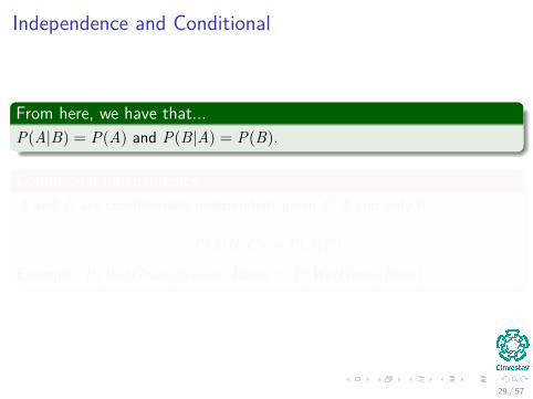
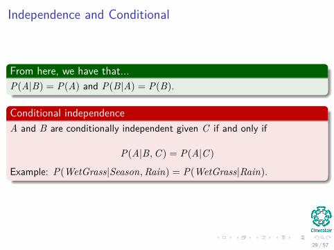
From here, we have that...P(A|B) = P(A) and P(B|A) = P(B).
Conditional independenceA and B are conditionally independent given C if and only if
P(A|B,C ) = P(A|C )
Example: P(WetGrass|Season,Rain) = P(WetGrass|Rain).
29 / 57
Independence and Conditional
From here, we have that...P(A|B) = P(A) and P(B|A) = P(B).
Conditional independenceA and B are conditionally independent given C if and only if
P(A|B,C ) = P(A|C )
Example: P(WetGrass|Season,Rain) = P(WetGrass|Rain).
29 / 57

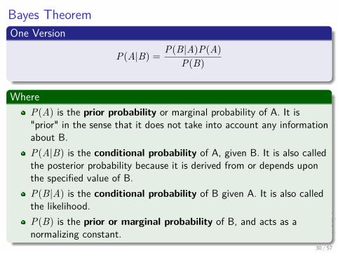
Bayes TheoremOne Version
P(A|B) = P(B|A)P(A)P(B)
WhereP(A) is the prior probability or marginal probability of A. It is"prior" in the sense that it does not take into account any informationabout B.P(A|B) is the conditional probability of A, given B. It is also calledthe posterior probability because it is derived from or depends uponthe specified value of B.P(B|A) is the conditional probability of B given A. It is also calledthe likelihood.P(B) is the prior or marginal probability of B, and acts as anormalizing constant.
30 / 57
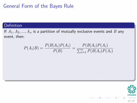
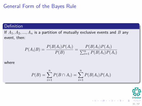
General Form of the Bayes Rule
DefinitionIf A1,A2, ...,An is a partition of mutually exclusive events and B anyevent, then:
P(Ai |B) = P(B|Ai)P(Ai)P(B) = P(B|Ai)P(Ai)∑n
i=1 P(B|Ai)P(Ai)
where
P(B) =n∑
i=1P(B ∩Ai) =
n∑i=1
P(B|Ai)P(Ai)
31 / 57
General Form of the Bayes Rule
DefinitionIf A1,A2, ...,An is a partition of mutually exclusive events and B anyevent, then:
P(Ai |B) = P(B|Ai)P(Ai)P(B) = P(B|Ai)P(Ai)∑n
i=1 P(B|Ai)P(Ai)
where
P(B) =n∑
i=1P(B ∩Ai) =
n∑i=1
P(B|Ai)P(Ai)
31 / 57

Example
SetupThrow two unbiased dice independently.
Let1 A =sum of the faces =82 B =faces are equal
Then calculate P (B|A)Look at the board
32 / 57
Example
SetupThrow two unbiased dice independently.
Let1 A =sum of the faces =82 B =faces are equal
Then calculate P (B|A)Look at the board
32 / 57

Example
SetupThrow two unbiased dice independently.
Let1 A =sum of the faces =82 B =faces are equal
Then calculate P (B|A)Look at the board
32 / 57

Another Example
We have the followingTwo coins are available, one unbiased and the other two headed
AssumeThat you have a probability of 3
4 to choose the unbiased
EventsA= head comes upB1= Unbiased coin chosenB2= Biased coin chosen
I Find that if a head come up, find the probability that the two headedcoin was chosen
33 / 57

Random Variables I
DefinitionIn many experiments, it is easier to deal with a summary variable thanwith the original probability structure.
ExampleIn an opinion poll, we ask 50 people whether agree or disagree with acertain issue.
Suppose we record a “1” for agree and “0” for disagree.The sample space for this experiment has 250 elements. Why?Suppose we are only interested in the number of people who agree.Define the variable X=number of “1” ’s recorded out of 50.Easier to deal with this sample space (has only 51 elements).
34 / 57

Thus...
It is necessary to define a function “random variable as follow”
X : S → R
Graphically
35 / 57

Thus...
It is necessary to define a function “random variable as follow”
X : S → R
Graphically
S
A
35 / 57

Random Variables II
How?What is the probability function of the random variable is being definedfrom the probability function of the original sample space?
Suppose the sample space is S = s1, s2, ..., snSuppose the range of the random variable X =< x1, x2, ..., xm >
Then, we observe X = xi if and only if the outcome of the randomexperiment is an sj ∈ S s.t. X(sj) = xj or
36 / 57
Random Variables II
How?What is the probability function of the random variable is being definedfrom the probability function of the original sample space?
Suppose the sample space is S = s1, s2, ..., snSuppose the range of the random variable X =< x1, x2, ..., xm >
Then, we observe X = xi if and only if the outcome of the randomexperiment is an sj ∈ S s.t. X(sj) = xj or
P(X = xj) = P(sj ∈ S |X(sj) = xj)
36 / 57
Example
SetupThrow a coin 10 times, and let R be the number of heads.
ThenS = all sequences of length 10 with components H and T
We have forω =HHHHTTHTTH ⇒ R (ω) = 6
37 / 57
Example
SetupThrow a coin 10 times, and let R be the number of heads.
ThenS = all sequences of length 10 with components H and T
We have forω =HHHHTTHTTH ⇒ R (ω) = 6
37 / 57

Example
SetupThrow a coin 10 times, and let R be the number of heads.
ThenS = all sequences of length 10 with components H and T
We have forω =HHHHTTHTTH ⇒ R (ω) = 6
37 / 57
Example
SetupLet R be the number of heads in two independent tosses of a coin.
Probability of head is .6
What are the probabilities?Ω =HH,HT,TH,TT
Thus, we can calculateP (R = 0) ,P (R = 1) ,P (R = 2)
38 / 57

Example
SetupLet R be the number of heads in two independent tosses of a coin.
Probability of head is .6
What are the probabilities?Ω =HH,HT,TH,TT
Thus, we can calculateP (R = 0) ,P (R = 1) ,P (R = 2)
38 / 57

Example
SetupLet R be the number of heads in two independent tosses of a coin.
Probability of head is .6
What are the probabilities?Ω =HH,HT,TH,TT
Thus, we can calculateP (R = 0) ,P (R = 1) ,P (R = 2)
38 / 57
Outline
1 Basic TheoryIntuitive FormulationAxiomsUnconditional and Conditional ProbabilityPosterior (Conditional) Probability
2 Random VariablesTypes of Random VariablesCumulative Distributive FunctionProperties of the PMF/PDFExpected Value and Variance
39 / 57

Types of Random Variables
DiscreteA discrete random variable can assume only a countable number of values.
ContinuousA continuous random variable can assume a continuous range of values.
40 / 57

Types of Random Variables
DiscreteA discrete random variable can assume only a countable number of values.
ContinuousA continuous random variable can assume a continuous range of values.
40 / 57
Properties
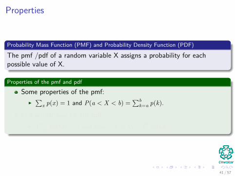
Probability Mass Function (PMF) and Probability Density Function (PDF)
The pmf /pdf of a random variable X assigns a probability for eachpossible value of X.
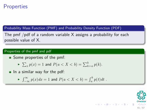
Properties of the pmf and pdf
Some properties of the pmf:I∑
x p(x) = 1 and P(a < X < b) =∑b
k=a p(k).
In a similar way for the pdf:I´∞−∞ p(x)dx = 1 and P(a < X < b) =
´ ba p(t)dt .
41 / 57

Properties
Probability Mass Function (PMF) and Probability Density Function (PDF)
The pmf /pdf of a random variable X assigns a probability for eachpossible value of X.
Properties of the pmf and pdf
Some properties of the pmf:I∑
x p(x) = 1 and P(a < X < b) =∑b
k=a p(k).
In a similar way for the pdf:I´∞−∞ p(x)dx = 1 and P(a < X < b) =
´ ba p(t)dt .
41 / 57

42 / 57
Outline
1 Basic TheoryIntuitive FormulationAxiomsUnconditional and Conditional ProbabilityPosterior (Conditional) Probability
2 Random VariablesTypes of Random VariablesCumulative Distributive FunctionProperties of the PMF/PDFExpected Value and Variance
43 / 57

Cumulative Distributive Function I
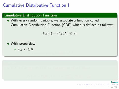
Cumulative Distribution FunctionWith every random variable, we associate a function calledCumulative Distribution Function (CDF) which is defined as follows:
FX (x) = P(f (X) ≤ x)
With properties:I FX(x) ≥ 0I FX(x) in a non-decreasing function of X .
ExampleIf X is discrete, its CDF can be computed as follows:
FX (x) = P(f (X) ≤ x) =∑N
k=1 P(Xk = pk).
44 / 57
Cumulative Distributive Function I
Cumulative Distribution FunctionWith every random variable, we associate a function calledCumulative Distribution Function (CDF) which is defined as follows:
FX (x) = P(f (X) ≤ x)
With properties:I FX(x) ≥ 0I FX(x) in a non-decreasing function of X .
ExampleIf X is discrete, its CDF can be computed as follows:
FX (x) = P(f (X) ≤ x) =∑N
k=1 P(Xk = pk).
44 / 57

Example: Discrete Function
.16
.48
.36
.16
.48
.36
1 2 1 2
1
45 / 57

Cumulative Distributive Function IIContinuous FunctionIf X is continuous, its CDF can be computed as follows:
F(x) =ˆ x
−∞f (t)dt.
RemarkBased in the fundamental theorem of calculus, we have the followingequality.
p(x) = dFdx (x)
NoteThis particular p(x) is known as the Probability Mass Function (PMF) orProbability Distribution Function (PDF).
46 / 57
Example: Continuous Function
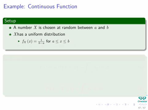
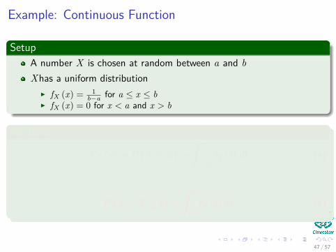
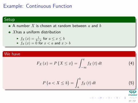
SetupA number X is chosen at random between a and bXhas a uniform distribution
I fX (x) = 1b−a for a ≤ x ≤ b
I fX (x) = 0 for x < a and x > b
We have
FX (x) = P X ≤ x =ˆ x
−∞fX (t) dt (4)
P a < X ≤ b =ˆ b
afX (t) dt (5)
47 / 57

Example: Continuous Function
SetupA number X is chosen at random between a and bXhas a uniform distribution
I fX (x) = 1b−a for a ≤ x ≤ b
I fX (x) = 0 for x < a and x > b
We have
FX (x) = P X ≤ x =ˆ x
−∞fX (t) dt (4)
P a < X ≤ b =ˆ b
afX (t) dt (5)
47 / 57
Example: Continuous Function
SetupA number X is chosen at random between a and bXhas a uniform distribution
I fX (x) = 1b−a for a ≤ x ≤ b
I fX (x) = 0 for x < a and x > b
We have
FX (x) = P X ≤ x =ˆ x
−∞fX (t) dt (4)
P a < X ≤ b =ˆ b
afX (t) dt (5)
47 / 57
Example: Continuous Function
SetupA number X is chosen at random between a and bXhas a uniform distribution
I fX (x) = 1b−a for a ≤ x ≤ b
I fX (x) = 0 for x < a and x > b
We have
FX (x) = P X ≤ x =ˆ x
−∞fX (t) dt (4)
P a < X ≤ b =ˆ b
afX (t) dt (5)
47 / 57

Example: Continuous Function
SetupA number X is chosen at random between a and bXhas a uniform distribution
I fX (x) = 1b−a for a ≤ x ≤ b
I fX (x) = 0 for x < a and x > b
We have
FX (x) = P X ≤ x =ˆ x
−∞fX (t) dt (4)
P a < X ≤ b =ˆ b
afX (t) dt (5)
47 / 57
Example: Continuous Function
SetupA number X is chosen at random between a and bXhas a uniform distribution
I fX (x) = 1b−a for a ≤ x ≤ b
I fX (x) = 0 for x < a and x > b
We have
FX (x) = P X ≤ x =ˆ x
−∞fX (t) dt (4)
P a < X ≤ b =ˆ b
afX (t) dt (5)
47 / 57
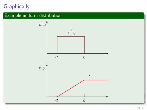
GraphicallyExample uniform distribution
1
48 / 57

Outline
1 Basic TheoryIntuitive FormulationAxiomsUnconditional and Conditional ProbabilityPosterior (Conditional) Probability
2 Random VariablesTypes of Random VariablesCumulative Distributive FunctionProperties of the PMF/PDFExpected Value and Variance
49 / 57

Properties of the PMF/PDF I
Conditional PMF/PDFWe have the conditional pdf:
p(y|x) = p(x, y)p(x) .
From this, we have the general chain rule
p(x1, x2, ..., xn) = p(x1|x2, ..., xn)p(x2|x3, ..., xn)...p(xn).
IndependenceIf X and Y are independent, then:
p(x, y) = p(x)p(y).
50 / 57

Properties of the PMF/PDF I
Conditional PMF/PDFWe have the conditional pdf:
p(y|x) = p(x, y)p(x) .
From this, we have the general chain rule
p(x1, x2, ..., xn) = p(x1|x2, ..., xn)p(x2|x3, ..., xn)...p(xn).
IndependenceIf X and Y are independent, then:
p(x, y) = p(x)p(y).
50 / 57
Properties of the PMF/PDF II
Law of Total Probability
p(y) =∑
xp(y|x)p(x).
51 / 57
Outline
1 Basic TheoryIntuitive FormulationAxiomsUnconditional and Conditional ProbabilityPosterior (Conditional) Probability
2 Random VariablesTypes of Random VariablesCumulative Distributive FunctionProperties of the PMF/PDFExpected Value and Variance
52 / 57

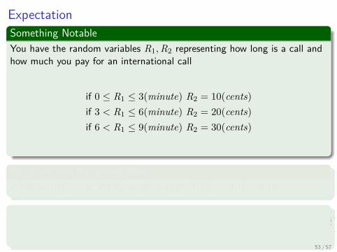
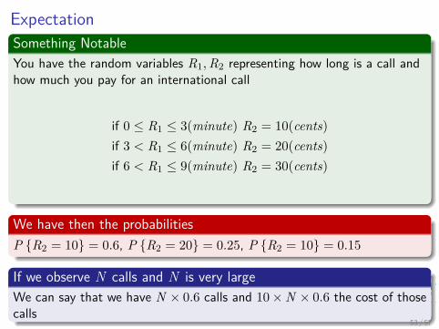
ExpectationSomething NotableYou have the random variables R1,R2 representing how long is a call andhow much you pay for an international call
if 0 ≤ R1 ≤ 3(minute) R2 = 10(cents)if 3 < R1 ≤ 6(minute) R2 = 20(cents)if 6 < R1 ≤ 9(minute) R2 = 30(cents)
We have then the probabilitiesP R2 = 10 = 0.6, P R2 = 20 = 0.25, P R2 = 10 = 0.15
If we observe N calls and N is very largeWe can say that we have N × 0.6 calls and 10×N × 0.6 the cost of thosecalls
53 / 57
Expectation
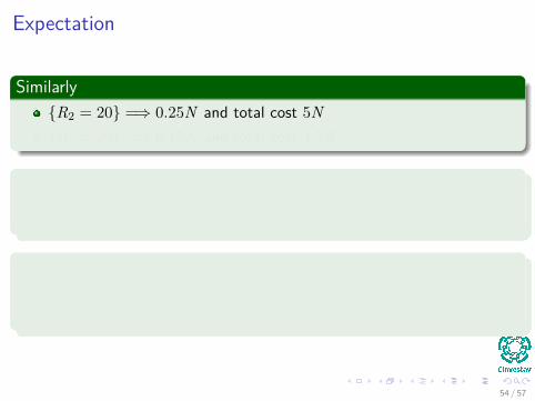
SimilarlyR2 = 20 =⇒ 0.25N and total cost 5NR2 = 20 =⇒ 0.15N and total cost 4.5N
We have then the probabilitiesThe total cost is 6N + 5N + 4.5N = 15.5N or in average 15.5 cents percall
The average10(0.6N)+20(.25N)+30(0.15N)
N = 10 (0.6) + 20 (.25) + 30 (0.15) =∑y yP R2 = y
54 / 57

Expectation
SimilarlyR2 = 20 =⇒ 0.25N and total cost 5NR2 = 20 =⇒ 0.15N and total cost 4.5N
We have then the probabilitiesThe total cost is 6N + 5N + 4.5N = 15.5N or in average 15.5 cents percall
The average10(0.6N)+20(.25N)+30(0.15N)
N = 10 (0.6) + 20 (.25) + 30 (0.15) =∑y yP R2 = y
54 / 57

Expectation
SimilarlyR2 = 20 =⇒ 0.25N and total cost 5NR2 = 20 =⇒ 0.15N and total cost 4.5N
We have then the probabilitiesThe total cost is 6N + 5N + 4.5N = 15.5N or in average 15.5 cents percall
The average10(0.6N)+20(.25N)+30(0.15N)
N = 10 (0.6) + 20 (.25) + 30 (0.15) =∑y yP R2 = y
54 / 57
Expected Value
DefinitionDiscrete random variable X : E(X) =
∑x xp(x).
Continuous random variable Y : E(Y ) =´
x xp(x)dx.
Extension to a function g(X)E(g(X)) =
∑x g(x)p(x) (Discrete case).
E(g(X)) =´∞
=∞ g(x)p(x)dx (Continuous case)
Linearity propertyE(af (X) + bg(Y )) = aE(f (X)) + bE(g(Y ))
55 / 57

Example
Imagine the followingWe have the following functions
1 f (x) = e−x , x ≥ 02 g (x) = 0, x < 0
FindThe expected Value
56 / 57

Example
Imagine the followingWe have the following functions
1 f (x) = e−x , x ≥ 02 g (x) = 0, x < 0
FindThe expected Value
56 / 57
Example
Imagine the followingWe have the following functions
1 f (x) = e−x , x ≥ 02 g (x) = 0, x < 0
FindThe expected Value
56 / 57
Example
Imagine the followingWe have the following functions
1 f (x) = e−x , x ≥ 02 g (x) = 0, x < 0
FindThe expected Value
56 / 57
Variance
DefinitionVar(X) = E((X − µ)2) where µ = E(X)
Standard DeviationThe standard deviation is simply σ =
√Var(X).
57 / 57

Variance
DefinitionVar(X) = E((X − µ)2) where µ = E(X)
Standard DeviationThe standard deviation is simply σ =
√Var(X).
57 / 57