03302--icwe14-2015-experimental and numerical evaluation of micrositing in complex areas- speed up...

1

14th International Conference on Wind Engineering – Porto Alegre, Brazil – June 21-26, 2015

Experimental and Numerical Evaluation of Micrositing in Complex Areas:

Speed up Effect Analysis

Mattuella, J.M.L.1, Loredo-Souza, A.M.

1 ,Vecina,T.D.J.

2 Petry, A.P.

2

1 Department of Civil Engineering, Laboratório de Aerodinâmica das Construções -LAC

2 Department of Mechanic Engineering

1,2Universidade Federal do Rio Grande do Sul-UFRGS, Porto Alegre, Brazil,

[email protected], [email protected], [email protected], [email protected],

1 ABSTRACT

Wind mapping is essential in various wind energy and wind engineering applications. For wind energy assessment purposes,

micrositing in complex areas represents challenging projects in the identification of intercurrent phenomena. Complex

topography such as ridges, hills and cliffs affects the airflow and direction, leading to deceleration or acceleration of the wind in

a short distance with growth of the turbulence intensity [1] [2] On the other hand, the wind velocity on the crest of the hills is

higher than on the plain area, since the wind increases with height and on the ridges, which allows a wide exposure to the

predominant wind from all directions. In addition to these factors, speed up effect occurs on the crest of topographic forms [2].

Such places may have favorable wind potential to install micrositings provided that the turbulence intensity determined by

topography is assessed [3]. In order to identify these special conditions, physical modeling in wind tunnel[4] and Computational

Fluid Dynamics-C.F.D are possible complementary tools [5]. This research presents the results of measurements and modeling

of speed-up effects for the mean horizontal velocity and the turbulence intensity profiles above the crest of eight symmetrical

hill models with slopes of 25o, 32o, 52o and 68o for two law exponents, corresponding to p=0.11 and p=0.23 [6]and compared

with those in the undisturbed (no-hill) boundary layer and those downwind of the hill. It focuses on comparing both methods to

analyze the speed up factor on the crest of the hills and to show how the incremental velocity may be decisive to install

micrositing on complex terrains.

KEY WORDS: Computational fluid dynamics, Complex terrains, Numerical simulation, Speed-up effect, Wind-

tunnel experiment, Wind-tunnel modeling

2 1.INTRODUCTION

Areas with diverse levels of complexity concerning topography, roughness and surrounding elements are increasingly common

in wind power projects. Complex micrositing may cause, at the same time, speed-up effect on the top of the hills, as well as flow

separation and recirculation downwind of the hill. While the wakes determined by topography and other turbines may represent

a challenging undertaking of the airflow, the speed up effect may present greater wind power across the flat areas, which

determine that such places can be references to install micrositings.

Terrain geometries can determine different flow patterns. Flow on complex terrain varies unpredictably, depending on daily and

seasonal variations on the thermal stability of flowing air masses. Geophysical phenomena such as thermal stratification and

Earth's rotation can add to the complexity [7]. The study about the development of the turbulent boundary layer is fundamental

for analyzing the micrositing, especially in areas characterized by variable topography. When the topographic characteristic is

sufficiently abrupt around 30 to 40%, a strong adverse pressure gradient occurs, which causes the deceleration at the base

windward. This fact gives rise to the local pressure adverse gradient. Thus, in order for a flow separation to take place, two

conditions are critical: the average velocity and its gradient must be zero, simultaneously, at the same point. These critical points

are called "separation points," and determine the instability of the flow and the start of the turbulence process. The different

wind profiles caused by turbulence intensity, the increase in the wind speed at the top of the hill, the extent of the recirculation

wake, and the reattachment length of the airflow are the key aspects for micrositing in complex areas.

Determinant variables in a project such as mean wind speed, extreme wind speed, turbulence intensity, and wake turbulence

remain not sufficiently defined by the traditional methods of wind energy assessment such as anemometric towers. In complex

mailto:[email protected]




2


areas, mainly in sloppy terrain, such measurement is not enough to analyze the assessment of the local wind resource, and

classical linear models fail to predict the extrapolation of the wind [3]. Anemometric towers provide a punctual measurement

with limited representativity in the surrounding. In order to have a comprehensive understanding of the intercurrent phenomena

of the airflow on the complex area, it is necessary to add a tool appropriate to airflow modeling, such as wind tunnel

experiments and C.F.D numerical analysis, where most of airflow parameters are possible to estimate[4] [5]. Hence, current

research in wind energy consists of field measurement in anemometric towers as a basic methodology for data measurement of

wind parameters, being numerical simulations and wind-tunnel experiment complementary tools, which are essential

methodologies to validate the wind flow and turbulence intensity profile in a micrositing layout.

2. STUDY ON FLOW OVER COMPLEX TERRAIN-Models and methodologies

The foundation for the study of atmospheric boundary layer flow over complex terrain was laid in the early 1970s. In 1975, an

analytical model for a two-dimensional flow over a low and isolated hill was developed [7]. The dimensions of the hill were

such that “d<<L”, where d is the height of elevation and L is the characteristic length of the hill in the direction of the flow. The

surface roughness zo was considered uniform and without separation of the airflow. The results obtained testified that the wind

speed and the cutting forces were proportional to the size, shape and roughness of the hill for slopes where “d/L <<1” and that

within these limits it would be possible to employ the equations of fluid movement [8].Such results remain valid until the

present day and have been confirmed by different methods. Basically, the flow over an isolated hill can be described by the

increment in wind speed at the crest of the hill, called the speed-up effect, and the associated deceleration of the flow on the

leeward side of hill, with the beginning of the formation of turbulence area and airflow detachment. Flow recirculation occurs at

the foot of the hill determining the so- called wind wake [8]. In the investigation of complex terrain, numerical models were

more extensively employed in the 70s. The results of that period suggested that the most relevant changes in the turbulence

intensity characteristics occur in the wake area downwind of the hill, where the transfer of energy to higher frequencies is more

evident [9]. In the 80s, the assessment of the flow behavior on large hills such as Blashaval, Askervein and others confirmed the

thesis of 1975 [8]. Britter, Hunt and Richards (1981) showed that the speed up effect at the crest of the hills was due to both the

slope and the surface roughness [10].

Kim et al. (1997) sought to validate mathematical models for airflow behavior forecast on hills with performing experiments in

tunnel and numerical simulations on complex terrain. Such experiments improved the understanding of the wake recirculation in

the downwind. Comparisons obtained by experimental results with numerical simulations matched both the average speed

values and pressure distribution [11].

In the 20th Century, Kim and Patel, H. showed the characterization of the airflow phenomenon, especially according to its

detachment and reattachment over topographic models in 2D and 3D analysis. The results obtained indicated that Reynolds

Stress increased rapidly in regions of the boundary layer with a strong adverse pressure gradient. Such increase remained even

when the flow reached the reattachment point, when turbulence decreased at the same time, and when the mean velocity profiles

started to recompose [12].

In the 21st century, Kastner and Rotach presented wind tunnel measurements compared with Laser-Doppler velocimetry in

2003. In this study, a detailed model of an urban landscape has been re-constructed in the wind tunnel and the flow structure

inside and above the urban canopy was investigated. Vertical profiles of all three velocity components were measured with a

Laser-Doppler velocimeter, and an analysis of the measured mean flow and turbulence profiles was carried out. The results

showed that the mean wind profiles above the urban structure follow a logarithmic wind law. Inside the roughness sub layer, a

local scaling approach results in good agreement between measured and predicted mean wind profiles [13].

Several methods are accessible to model the wind in the atmospheric boundary layer (ABL) both at meso and at micro scale

levels. Micro scale models focus on the atmospheric processes at the lowest part of the ABL and do not exceed the length of

one kilometer. In this case the Earth’s rotation is not taken into consideration and the flow is commonly considered neutral. In

this scale the experiments are developed in a wind tunnel and constructed through numerical methods to predict wind fields in

the surface layer [12].

The numerical methods, based on mass-conservation and Navier-Stokes equations, Computational Fluid Dynamics (CFD)

models, such simulate de ABL modeling turbulent flow with the use of Reynolds Averaged Navier Stokes (RANS)

or Large Eddy Simulation (LES) [14].

Research in tunnels. play an important role on the definition and validation of micrositings, especially in the study of

3


the wind velocity profiles, turbulence intensity profiles and wakes, both coming from the topography, as well as

from the other wind turbines. Modelling and evaluation of the wind velocity, the turbulence intensity profiles on

complex micrositings for wind power assessment using numerical and experimental methodology compared has

been recently reported by Mattuella, Loredo-Souza and Petry [5].

2.1 Speed up effect

Speed up effect is an increment in velocity that often occurs on the top and near the top upwind and downwind of topographic

features, such as escarpments and ridges. This happens because the wind is compressed upwind, and when it reaches the top of

the hill, it expands in the low pressure area on the lee side of the hill. The velocity over the topography is written according to

Eq 01.

),()(),( zxUzUozxU

Eq.(01)

where

)(xUois the mean velocity of the incoming flow upstream the terrain feature.

The speed-up effect may be quantified by the fractional speed-up ratio, which is defined as the fraction of the change in the

velocity in relation to approaching undisturbed velocity at each height and as follows Eq. 02 [15].

)(

),(

)(

)(),(),(

zUo

zxU

zUo

zUozxUzxS

Eq.(02)

3.THE EXPERIMENTAL SET-UP

The present experiments were conducted at Joaquim Blessmann Atmospheric Boundary Layer Wind Tunnel located at

Laboratório de Aerodinâmica das Construções(Construction Aerodynamic Laboratory) of Universidade Federal do Rio Grande

do Sul(Federal University of Rio Grande do Sul), Brazil. The LAC Wind Tunnel is a closed return low speed wind tunnel,

specifically projected for the dynamic and static studies on civil construction models. Its design allows the simulation of the

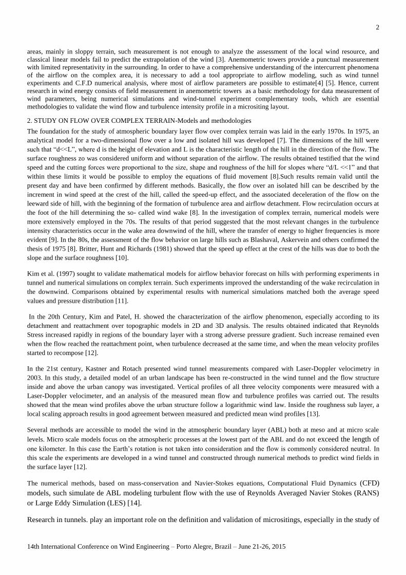
natural winds main characteristics. It has a length/height ratio on the main test section greater than 10 and dimensions of 1.30 m

x 0.90 m x 9.32 m (width x height x length), as shown in Figure 01. The maximum wind speed in this chamber, with soft and

uniform flow is 42 m s^-1 (150 km h^-1). The propeller is driven by a 100HP electric motor and the wind speed is controlled by

a frequency inverter. The data acquisition is performed using a Dantec Dynamics anemometer, System 90 Streamline N S. The

system uses a constant temperature anemometer as reference. The hot wire probe and a calibrator are automatically integrated to

the computer. The frame also has an input for a temperature sensor, which is designed to measure the flow temperature (fast

fluctuations).The signal registration was done by the probe and the effective data acquisition was performed with the use of the

Stream Ware application software, from same brand. The frequency was 2 kHz, and the acquisition period was 64s. The data

acquisition program is from Dantec Dynamic, and it also enables its own calibration and data accumulation. Mano Air 500

equipment measures the pressure difference between the piezometric rings, which are situated at the entrance of the tunnel and

measure the average temperature inside it at an interval of 65s [5].

The Boundary Layer Wind Tunnel Prof. Joaquim Blessman – floor plan is shown in Figure 01.

Figure 1. Boundary Layer Wind Tunnel Prof. Joaquim Blessmann – Floor Plan

4


3.1 Experimental model

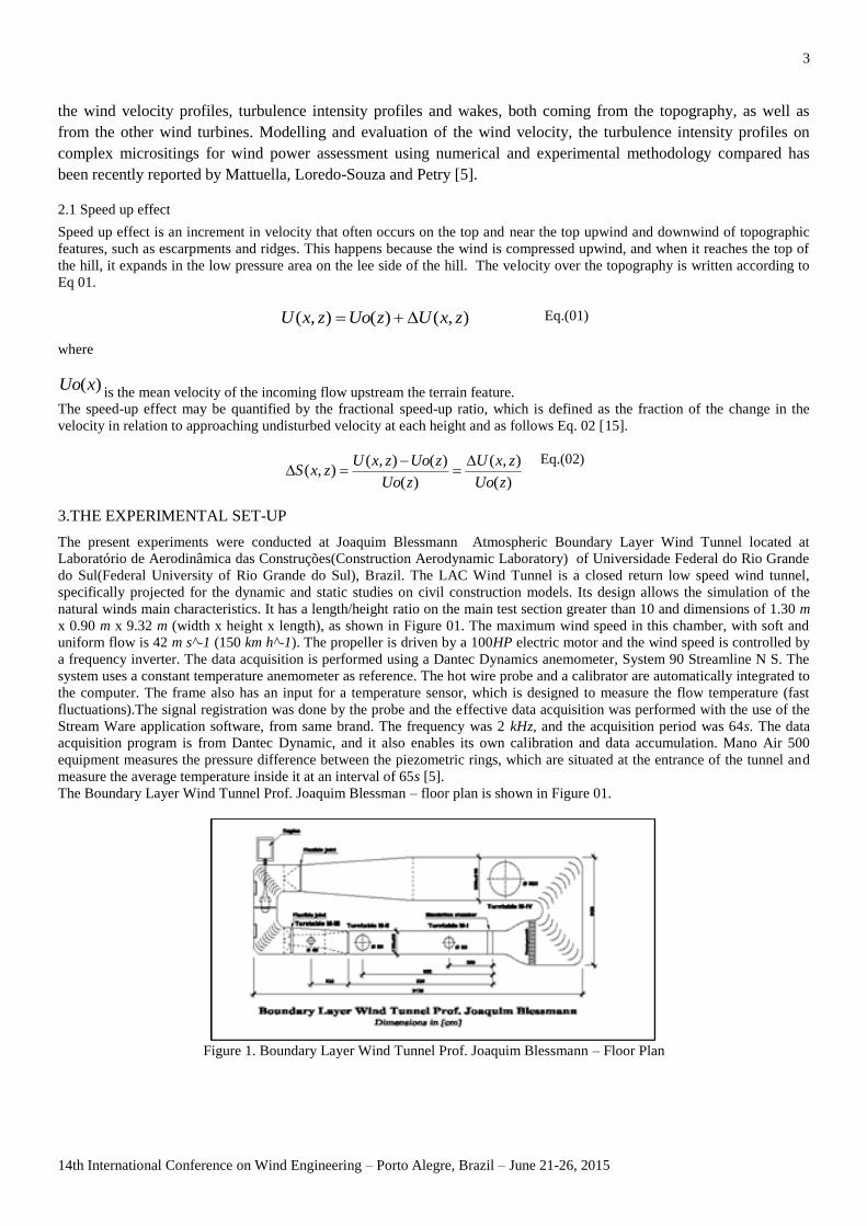
The experimental program performed at the cited tunnel focused on the boundary layer behavior at the crest of the symmetrical

hill models with different slopes for two types of terrain, according to NBR standard, Category I - plain and Categories III/IV -

moderated roughness. For this examination were employed eight hills models, (four 2D and four 3D) in a reduced 1:1000 scale.

The models were constructed in layers in order to minimize the effects of the Reynolds number. This technique is used in

several laboratories around the world. The experimental measurements were realized with 20 (twenty) height measurements. For

each height a total of 131,072 wind speed values were collected. Figure 2 (a,b,c,d)shows the 2D/3D models inside the test

chamber [16].

2D(a) 3D(b)

2D(a) 3D(b)

(a)Model A – 25º slope

(b)Model B – 32º slope

2D(a) 3D(b)

2D(a) 3D(b)

(c)Model C – 52º slope (d)Model D – 64º slope

Figure. 2. Experimental Models 25o, 32

o, 52

o and 64

o in 2D/3D inside the wind tunnel chamber.

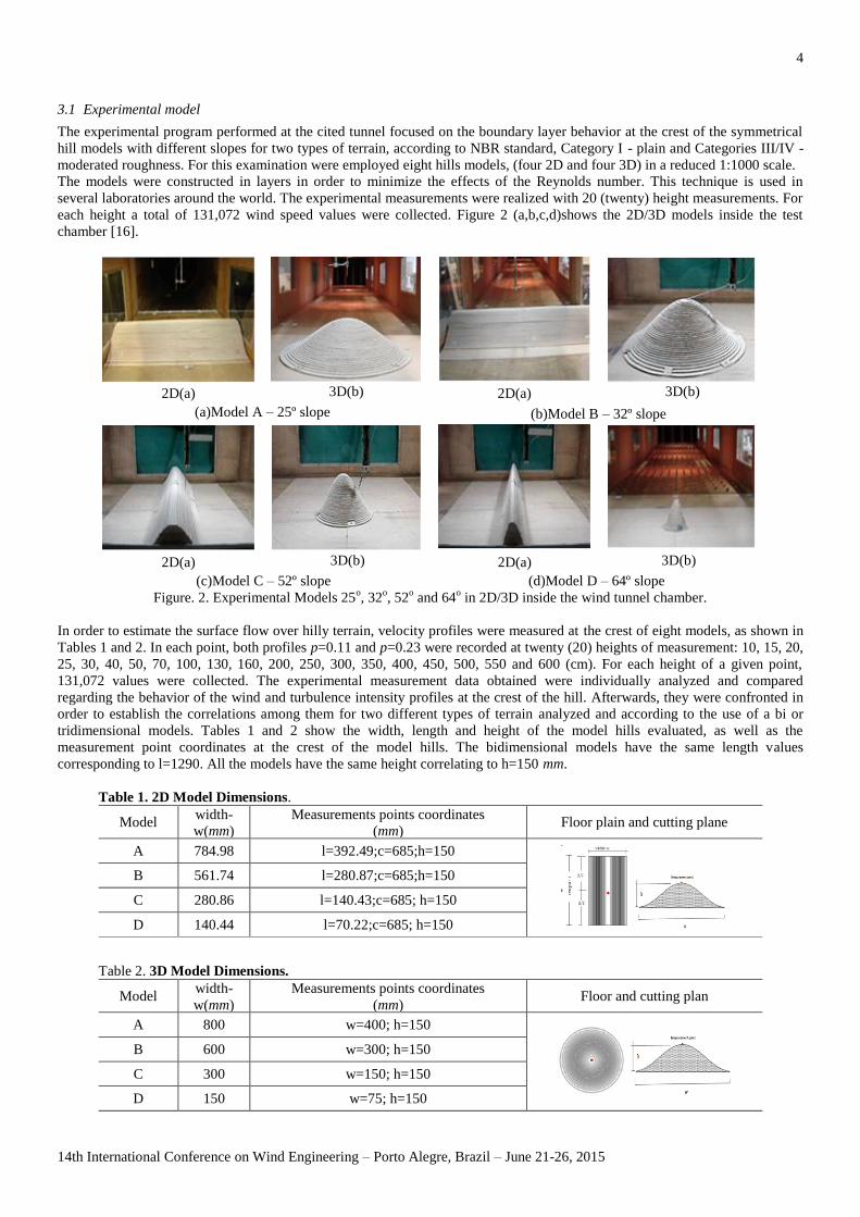
In order to estimate the surface flow over hilly terrain, velocity profiles were measured at the crest of eight models, as shown in

Tables 1 and 2. In each point, both profiles p=0.11 and p=0.23 were recorded at twenty (20) heights of measurement: 10, 15, 20,

25, 30, 40, 50, 70, 100, 130, 160, 200, 250, 300, 350, 400, 450, 500, 550 and 600 (cm). For each height of a given point,

131,072 values were collected. The experimental measurement data obtained were individually analyzed and compared

regarding the behavior of the wind and turbulence intensity profiles at the crest of the hill. Afterwards, they were confronted in

order to establish the correlations among them for two different types of terrain analyzed and according to the use of a bi or

tridimensional models. Tables 1 and 2 show the width, length and height of the model hills evaluated, as well as the

measurement point coordinates at the crest of the model hills. The bidimensional models have the same length values

corresponding to l=1290. All the models have the same height correlating to h=150 mm.

Table 1. 2D Model Dimensions.

Model width-

w(mm)

Measurements points coordinates

(mm) Floor plain and cutting plane

A 784.98 l=392.49;c=685;h=150

B 561.74 l=280.87;c=685;h=150

C 280.86 l=140.43;c=685; h=150

D 140.44 l=70.22;c=685; h=150

Table 2. 3D Model Dimensions.

Model width-

w(mm)

Measurements points coordinates

(mm) Floor and cutting plan

A 800 w=400; h=150

B 600 w=300; h=150

C 300 w=150; h=150

D 150 w=75; h=150

5


4. NUMERICAL METHODOLOGY

The numerical simulation in this paper uses the method of finite volume to solve the Reynolds Averaged Navier-Stokes

equations, two turbulence models are used, the k-ε and the k-ω SST [16]. Both simulations are performed through the ANSYS-

Fluent 13.0 software. The working fluid is air, as an ideal gas at 25 °C. The method of solution used is Pressure Velocity

Coupling SIMPLE and the convergence criterion is set at 1x10-5.

The simulations are developed through the computational representation of the same geometries of the experimental analysis in

Prof. Joaquim Blessmann wind tunnel [8], as shown in Figure 3 and Figure 4.

(a) (b)

Figure 3: Computational Model 2D.

(a) (b)

Figure 4. Computational Model 3D.

The computational domain is discretized in finite volumes. Ansys ICEM-13.0 software was used to generate the mesh, which

will then be used for the simulations and for obtaining the results. The discretization is done using hexahedral finite volumes

with refinement near the surface. For each case, two-dimensional and tree-dimensional hills, four meshes are created varying the

number of finite volumes, in order to evaluate their quality, for both cases the mesh adopted have about 1,500,000 of volumes,

Figure 6 represents the discretized computational domain.

Figure 5 – Computational domain, 2D and 3D model meshes

As boundary condition of inlet, it is used the velocity profile with the same characteristics of the experiments in the wind tunnel

to reproduce results closer to the experimental data. According to experimental data, the bottom of the tunnel elements have

such roughness that the power law expressed with p = 0.23 and the upper part where no roughness elements is used a value of p

= 0.11 for the velocity profile. The input profile (Eq. 03 and Eq. 04) is created in C language as User Define Function (UDF).

The tunnel walls are made of wood, so the prescribed roughness set for wood is 0.0009 m, and the ground uses a wall, no-slip,

boundary condition.

( ) |(

)

| Eq. (03)

6


( ) |(

)

| Eq. (04)

Table 3 shows the CFD cases analyzed, for 2D model steady state flow is solved with the two turbulence models, for

3D model five case are presented, two cases for steady state and three cases for transient analysis. At 3D model Case

V is simulated with prescribed roughness at the model surface.

Table 3 – CFD analyzed cases.

Case Regime esc. Modelo Turb.

I 2D Steady k-ε

II k-ω SST

III

3D

Steady

k-ε

IV k-ω SST

V k-ω c/ rug.

VI Transient k-ε

VII k-ω SST

5. RESULTS AND DISCUSSION

The experimental profiles were compared regarding the behavior of the wind profile at the crest of the hill in order to establish

the correlations among them for Categories I and III-IV, related to the power law exponents p=0.11 and p=0.23 according to

Brazilian Standard Code NBR 6123[6].in 2D/3D. To calculate the mean velocity, it was considered the value of the basic wind

velocity (vo m/s), and the normalization of the roughness factor according to NBR 6123[5]. The velocity was normalized by Δpa

(mmH2O). The profiles of mean stream-wise velocity over the crest of the models are plotted in Fig 6 and show the comparison

among the experimental profile measurements at the crest of the hills models, for each model separately.

(a) Model A - 25º (b) Model B - 32º

(a) Model C - 52º (b) Model D - 64º

Figure 6. Comparative study of experimental wind profiles among the models for p=0.11 and p=0.23 in 2D/3D.

7


In this scenery one can analyze and compare the speed-up effect, which occurs in such points. According to the graphs one can

see that the most significant difference in measurements performed on the 2D models comparatively to 3D models mainly

occurs from Model C on and for both to p=0.11 and p=0.23. One can also see that the best speed up configuration occurs in

Models D for p=0.23.

Next, the profiles of mean stream-wise velocity over the crest of the models are plotted in comparison separately p=0.11 and

p=0.23 in Fig. 7(a) and (b).

(a) p=0.11-2D/3D (b) p=0.23-2D/3D

Figure 7 Comparative study of experimental wind profiles among the models in 2D/3D for p=0.11 and p=0.23.

One can see in Figures 7 (a)(b) that models in 2D may lead to a greater difference in the wind velocity profiles from Model C

on.

In the sequence, the measured profiles above the crest of the hill were contrasted with the undisturbed stream flow for

p=0.11/p=0.23 with focus on the speed-up modeling and how it may vary under different conditions (slopes, roughness and

2D/3D). Figure 8(a,b,c,d) presents the comparison study for each model.

(a)Model A-25º (b)Model B-32º

(c)Model C-52º

(d)Model D-64º

Fig. 8 Comparative study of experimental wind profiles with the reference profiles for p=0.11 and p=0.23, both in 2D/3D

models.

8


According to Figure 8, in all the models for two types of potential law and for 2D/3D we can identify that the mean horizontal

velocity profiles at the crest increased in comparison with reference profiles on a plain terrain. Such incremental velocity on the

crest of hills is named speed up effect. It is possible to verify that the 3D measurements show more intense speed up effect,

being more evident in Models C and D, for both p=0.11 and p=0.23.

The speed up factor varied from 7.14% to 14.28% for p=0.11 and from 20% to 25% for p=0.23, being the best definition in

models C and D and in 3D.

The flow at the crest of the hills is subjected to the influence of an adverse pressure gradient, which occurs due to the airflow

detachment at the crest of the hill and determines the turbulence intensity. It is necessary to consider these parameters to define

the installation of the micrositing at the crest of the hills. Turbulence intensity is calculated according to Eq. 05, where σu is

standard deviation of the wind speed and U(z) is the mean wind speed profile.

)()(

zUzI u

u

Eq.(05)

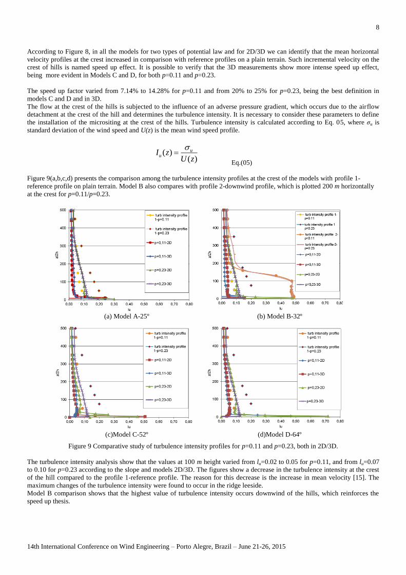
Figure 9(a,b,c,d) presents the comparison among the turbulence intensity profiles at the crest of the models with profile 1-

reference profile on plain terrain. Model B also compares with profile 2-downwind profile, which is plotted 200 m horizontally

at the crest for p=0.11/p=0.23.

(a) Model A-25º (b) Model B-32º

(c)Model C-52º

(d)Model D-64º

Figure 9 Comparative study of turbulence intensity profiles for p=0.11 and p=0.23, both in 2D/3D.

The turbulence intensity analysis show that the values at 100 m height varied from lu=0.02 to 0.05 for p=0.11, and from lu=0.07

to 0.10 for p=0.23 according to the slope and models 2D/3D. The figures show a decrease in the turbulence intensity at the crest

of the hill compared to the profile 1-reference profile. The reason for this decrease is the increase in mean velocity [15]. The

maximum changes of the turbulence intensity were found to occur in the ridge leeside.

Model B comparison shows that the highest value of turbulence intensity occurs downwind of the hills, which reinforces the

speed up thesis.

9


Numerical results for the velocity profile on the top of the hill, for the seven different cases are, compared with

experimental data, as shown in Figure 10. In the simulation of flow over 2D geometry with turbulence models

k-ε and k-ω SST results are almost the same for the profiles, the mean difference between the first model results and

experimental values are 5.07% and 6.38% for the last one. For the 3D hill, results for the velocity profile obtained

with turbulence models k-ε, k-ω SST and k-ω SST with roughness prescribed at the surface of the model are

presented, and the mean difference between experimental data and numerical values are 3.51% for the first model,

3.44% for the second one and 2.3% for the k-ω SST with roughness prescribed. It is possible to verify that the best

results are obtained for the simulations with the k-ω SST with roughness prescribed at the surface of the model.

Figure 10. Numerical and experimental velocity profiles over the point at top of the 2D and 3D models.

Numerical results are suitable to analyze the flow topology. Figure 11 shows the velocity field at a plane over the

center line of the domain for both cases of the 2D model, Case I and Case II, defined in Table 3. It is possible to

identify in the images the speed-up over the top at the hill and the wake region after the model, with slow velocity.

At the velocity field is possible to observe differences of the results obtained with the two turbulence models,

especially the length of the recirculation region of the wake.

(a) (b)

Figure 11. Velocity field for the 2D model, at the medium plane obtained with k-ε (a) and k-ω SST (b) turbulence

model.

The velocity vectors in the region near the wake for cases I and II are presented at Figure 13. The velocities obtained

for Case II are smaller than for Case I.

10


(a) (b)

Figure 12. Velocity vectors for the 2D model, at the medium plane, near wake, obtained with k-ε (a) and k-ω SST

(b) turbulence model.

Figure 13 shows the velocity field at a plane over the center line of the domain for both cases of the 3D model, Case

V, and Figure 15 shows numerical results for Cases VI and VII. Results for Cases III and IV (steady state) are

almost the same as transient Cases VI and VII, respectively, so the velocity fields of those cases are not shown. As

in 2D model simulation it is possible to identify the speed-up over the top at the hill and the wake region after the

model. However, the use of different turbulence models results in a more significant difference at the velocity field

for the 3D model, specially on the height and length of the wake, Figure 14(a) and 15(b).

Figure 13. Velocity field for the 3D model, at the medium plane obtained with k-ω SST turbulence model and

prescribed roughness at the model surface.

(a) (b)

Figure 14. Velocity field for the 3D model, at the medium plane obtained with k-ε (a) and k-ω SST (b) turbulence

model.

11


The roughness length imposed in Case V (Figure 14 b) results in relevant differences at the wake topology when

compared to the similar Case VII (Figure 14 b) with smooth surface.

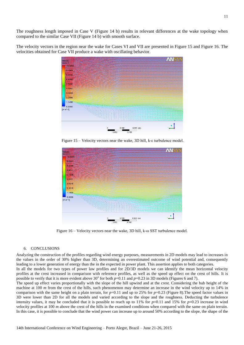
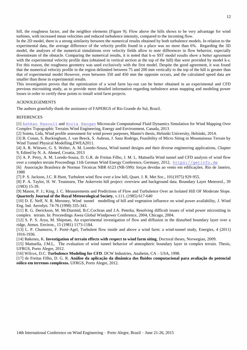
The velocity vectors in the region near the wake for Cases VI and VII are presented in Figure 15 and Figure 16. The

velocities obtained for Case VII produce a wake with oscillating behavior.

Figure 15 – Velocity vectors near the wake, 3D hill, k-ε turbulence model.

Figure 16 – Velocity vectors near the wake, 3D hill, k-ω SST turbulence model.

6. CONCLUSIONS

Analyzing the construction of the profiles regarding wind energy purposes, measurements in 2D models may lead to increases in

the values in the order of 30% higher than 3D, determining an overestimated outcome of wind potential and, consequently

leading to a lower generation of energy than the in the expected in power plant. This assertion applies to both categories.

In all the models for two types of power law profiles and for 2D/3D models we can identify the mean horizontal velocity

profiles at the crest increased in comparison with reference profiles, as well as the speed up effect on the crest of hills. It is

possible to verify that it is more evident above 30o for both p=0.11 and p=0.23 in 3D models (Figures 6 and 7).

The speed up effect varies proportionally with the slope of the hill upwind and at the crest. Considering the hub height of the

machine at 100 m from the crest of the hills, such phenomenon may determine an increase in the wind velocity up to 14% in

comparison with the same height on a plain terrain, for p=0.11 and up to 25% for p=0.23 (Figure 8).The speed factor values in

3D were lower than 2D for all the models and varied according to the slope and the roughness. Deducting the turbulence

intensity values, it may be concluded that it is possible to reach up to 11% for p=0.11 and 15% for p=0.23 increase in wind

velocity profiles at 100 m above the crest of the hills in the examined conditions when compared with the same on plain terrain.

In this case, it is possible to conclude that the wind power can increase up to around 50% according to the slope, the shape of the

12


hill, the roughness factor, and the neighbor elements (Figure 9). Flow above the hills shows to be very advantage for wind

turbines, with increased mean velocities and reduced turbulence intensity, compared to the incoming flow.

In the 2D model, there is a strong similarity between the numerical results obtained by both turbulence models. In relation to the

experimental data, the average difference of the velocity profile found in a place was no more than 6%. Regarding the 3D

model, the analyses of the numerical simulations over velocity fields allow to note differences in flow behavior, especially

downstream of the obstacle. Comparing the numerical results, it is noted that k-ω SST model results show a better agreement

with the experimental velocity profile data (obtained in vertical section at the top of the hill) that were provided by model k-ε.

For this reason, the roughness geometry was used exclusively with the first model. Despite the good agreement, it was found

that the numerical velocity profile in the region delimited between 75 and 200 mm vertically to the top of the hill is greater than

that of experimental model However, even between 350 and 450 mm the opposite occurs, and the calculated speed data are

smaller than those in experimental results.

This investigation proves that the optimization of a wind farm lay-out can be better obtained in an experimental and CFD

previous micrositing study, as to provide more detailed information regarding turbulence areas mapping and modeling power

losses in order to certify these points to install wind farm projects.

ACKNOLEGEMENTS

The authors gratefully thank the assistance of FAPERGS of Rio Grande do Sul, Brazil.

REFERENCES

[1] Ashkan Rasouli and Horia Hangan Microscale Computational Fluid Dynamics Simulation for Wind Mapping Over

Complex Topographic Terrains Wind Engineering, Energy and Environment, Canada, 2013

[2] Sointu, Lida, Wind profile assessment for wind power purposes, Master's thesis, Helsinki University, Helsinki, 2014.

[3] B. Conan, S. Buckingham, J. van Beeck, S. Aubrun, J. Sanz Rodrigo, Feasibility of Micro Siting in Mountainous Terrain by

Wind Tunnel Physical Modelling,EWEA2011.

[4] A. R. Wittwer, G. S. Welter, A. M. Loredo-Souza, Wind tunnel designs and their diverse engineering applications, Chapter

9, Edited by N. A. Ahmed, Croatia, 2013

[5] A. P. Petry, A. M. Loredo-Souza, D. G.R. de Freitas Filho, J. M. L. Mattuella Wind tunnel and CFD analysis of wind flow

over a complex terrain Proceedings 11th German Wind Energy Conference, Germany, 2012, https://getinfo.de

[6] Associação Brasileira de Normas Técnicas NBR 6123 (NB-599): forças devidas ao vento em edificações. Rio de Janeiro,

1988

[7] P. S. Jackson, J.C. R Hunt, Turbulent wind flow over a low hill, Quart. J. R. Met Soc., 101(1975) 929-955.

[8] P. A. Taylor, H. W. Teunissen, The Askervein hill project: overview and background data. Boundary Layer Meteorol., 39

(1983) 15-39.

[9] Mason, P. J.; King, J. C. Measurements and Predictions of Flow and Turbulence Over an Isolated Hill OF Moderate Slope.

Quarterly Journal of the Royal Meteorological Society, v.111, (1985) 617-640

[10] D. E. Neff, N. R. Meroney, Wind tunnel modelling of hill and vegetation influence on wind power availability, J. Wind

Eng. Ind. Aerodyn. 74-76 (1998) 335-343.

[11] R. G. Derickson, M. McDiarmid, B.C.Cochran and J.A. Peterka, Resolving difficult issues of wind power micrositing in

complex terrain. In: Proceedings Awea Global Windpower Conference, 2004, Chicago, 2004.

[12] S. P. S. Arya, M. Shipman, An experimental investigation of flow and diffusion in the disturbed boundary layer over a

ridge, Atmos. Environ., 15 (1981) 1173-1184.

[13] L. P. Chamorro, F. Porté-Agel, Turbulent flow inside and above a wind farm: a wind-tunnel study, Energies, 4 (2011)

1916-1936.

[14] Røkenes, K. Investigation of terrain effects with respect to wind farm siting, Doctoral theses, Norwegian, 2009.

[15] Mattuella, J.M.L, The evaluation of wind tunnel behavior of atmospheric boundary layer in complex terrain. Thesis,

UFRGS, Porto Alegre, 2012.

[16] Wilcox, D.C. Turbulence Modeling for CFD. DCW Industries, Anaheim, CA – USA, 1998.

[17] de Freitas Filho, D. G. R. Análise da aplicação da dinâmica dos fluidos computacional para avaliação do potencial

eólico em terrenos complexos. UFRGS, Porto Alegre, 2012.

http://solarenergyengineering.asmedigitalcollection.asme.org/solr/searchresults.aspx?author=Ashkan+Rasouli&q=Ashkan+Rasouli

http://solarenergyengineering.asmedigitalcollection.asme.org/solr/searchresults.aspx?author=Horia+Hangan&q=Horia+Hangan

https://getinfo.de/

03302--icwe14-2015-experimental and numerical evaluation of micrositing in complex areas- speed up...

Documents

wind velocity

wind tunnel4

predominant wind

windtunnel modeling

wind engineering applications

wind power projects

various wind energy

wind tunnel experiment