05-06400 book.indb - united nations statistics division
TRANSCRIPT

ST/ESA/STAT/SER.F/98
asdfUnited NationsNew York, 2008
Studies in Methods Series F No. 98
Designing Household Survey Samples: Practical Guidelines
Department of Economic and Social Affairs
Statistics Division

Department of Economic and Social AffairsThe Department of Economic and Social Affairs o f the United Nations Secretariat is a vital inter-face between global policies in the economic, social and environmental spheres and national action. The Department works in three main interlinked areas: (i) it compiles, generates and analyses a wide range of economic, social and environmental data and information on which States Members of the United Nations draw to review common problems and to take stock of policy options; (ii) it faci-litates the negotiations of Member States in many intergovernmental bodies on joint courses of action to address ongoing or emerging global challenges; and (iii) it advises interested Governments on the ways and means of translating policy frameworks developed in United Nations conferences and summits into programmes at the country level and, through technical assistance, helps build national capacities.
NoteThe designations employed and the presentation of the material in this publication do not imply the expression of any opinion whatsoever on the part of the Secretariat of the United Nations concerning the legal status of any country, territory, city or area or of its authorities, or concerning the delimitation of its frontiers or boundaries.
The term “country” as used in the text of this publication also refers, as appropriate, to territories or areas.
The designations “developed” and “developing” countries or areas and “more developed”, “less develo-ped” and “least developed” regions are intended for statistical convenience and do not necessarily ex-press a judgement about the stage reached by a particular country or area in the development process.
Symbols of United Nations documents are composed of capital letters combined with figures. Mention of such a symbol indicates a reference to a United Nations document.
ST/ESA/STAT/SER.F/98
ISBN 978-92-1-161495-4
United Nations Publication Sales No. E.06.XVII.13
Copyright © United Nations, 2008 All rights reserved

iii
Preface
The main purpose of Designing Household Survey Samples: Practical guidelines is to serve as a handbook that includes in one publication the main sample survey design issues that can conven‑iently be referred to by practising national statisticians, researchers and analysts involved in sample survey work and activities in countries. Methodologically sound techniques that are grounded in statistical theory are used in this handbook, implying the use of probability sampling at each stage of the sample selection process. A well‑designed household survey that is properly implemented can generate necessary information of sufficient quality and accuracy with speed and at a relatively low cost.
The contents of this publication can also be used, in part, as a training guide for introductory courses in sample survey design at various statistical training institutions that offer courses in applied statistics, especially survey methodology.
In addition, this publication has been prepared to complement other publications dealing with sample survey methodology issued by the United Nations, like the recent publication entitled Household Sample Surveys in Developing and Transition Countries1 and the series under the National Household Survey Capability Programme (NHSCP).
More specifically, the objectives of the handbook are to:
(a) Provide, in one publication, basic concepts and methodologically sound procedures for designing samples for, in particular, national‑level household surveys, emphasizing applied aspects of household sample design;
(b) Serve as a practical guide for survey practitioners in designing and implementing efficient household sample surveys;
(c) Illustrate the interrelationship of sample design, data collection, estimation, processing and analysis;
(d) Highlight the importance of controlling and reducing non‑sampling errors in household sample surveys.
While a sampling background will be helpful to users of the handbook, others with a general knowl‑edge of statistical and mathematical concepts should also be able to use it and apply its contents with little or no assistance. This is because one of the key aims of the handbook is to present material in a practical, hands‑on format as opposed to stressing the theoretical aspects of sampling. Theoretical underpinnings, however, are provided when necessary. It is expected that a basic understanding of
1 Studies on Methods; No. 96 (United Nations publication, Sales No. E.05.XVII.6).

iv Designing Household Survey Samples: Practical Guidelines
algebra is all that is needed to follow the presentation easily and to apply the techniques. Accordingly, numerous examples are provided to illustrate the concepts, methods and techniques.
A number of experts contributed to the preparation of the handbook. Mr. Anthony Turner, Sampling Consultant, drafted chapters 3, 4 and 5 and reviewed the final consolidated document; Mr. Ibrahim Yansaneh, Deputy Chief, Cost of Living Division, International Civil Service Commission, drafted chapters 6 and 7; and Mr. Maphion Jambwa, Statistician at the Southern African Development Community Secretariat, drafted Chapter 9.
Mr. Jeremiah Banda, United Nations Statistics Division, who served as the project’s editor‑in‑chief and technical coordinator, authored chapter 1, 2 and 8 including annex I. Ms. Clare Menozzi helped edit the first draft of various chapters; and Ms. Bizugenet Kassa provided invaluable secretarial assist‑ance while Ms. Pansy Benjamin assisted in harmonizing the formats.
The draft chapters were reviewed by an Expert Group Meeting organized by the Statistics Division, held in New York from 3 to 5 December 2003. The list of participants is contained in annex II. In addition, the handbook was peer reviewed by Dr. Alfredo Bustos, Ms. Ana María Landeros and Mr. Eduardo Ríos, from the Mexican National Institute of Statistics, Geography and Informatics (INEGI), who provided very valuable comments.
Paul CheungDirectorUnited Nations Statistics DivisionDepartment for Economic and Social Affairs

v
Contents
Page
Preface. . . . . . . . . . . . . . . . . . . . . . . . . . . . . . . . . . . . . . . . . . . . . . . . . . . . . . . . . . . . . . . . . . . . iii
Chapter 1
Sources of data for social and demographic statistics
1.1. Introduction . . . . . . . . . . . . . . . . . . . . . . . . . . . . . . . . . . . . . . . . . . . . . . . . . . . . . . . . . . . . . . . 1 1.2. Data sources . . . . . . . . . . . . . . . . . . . . . . . . . . . . . . . . . . . . . . . . . . . . . . . . . . . . . . . . . . . . . . . 1 1.2.1. Household surveys . . . . . . . . . . . . . . . . . . . . . . . . . . . . . . . . . . . . . . . . . . . . . . . . . . . 1 1.2.2. Population and housing censuses . . . . . . . . . . . . . . . . . . . . . . . . . . . . . . . . . . . . . . . . 4 1.2.3. Administrative records . . . . . . . . . . . . . . . . . . . . . . . . . . . . . . . . . . . . . . . . . . . . . . . . 5 1.2.4. Complementarities of the three data sources . . . . . . . . . . . . . . . . . . . . . . . . . . . . . . . 5 1.2.5. Concluding remarks . . . . . . . . . . . . . . . . . . . . . . . . . . . . . . . . . . . . . . . . . . . . . . . . . . 7 References and further reading . . . . . . . . . . . . . . . . . . . . . . . . . . . . . . . . . . . . . . . . . . . . . . . . . 7
Chapter 2
Planning and execution of surveys
2.1. Planning of surveys. . . . . . . . . . . . . . . . . . . . . . . . . . . . . . . . . . . . . . . . . . . . . . . . . . . . . . . . . . 9 2.1.1. Objectives of a survey . . . . . . . . . . . . . . . . . . . . . . . . . . . . . . . . . . . . . . . . . . . . . . . . . 9 2.1.2. Survey universe. . . . . . . . . . . . . . . . . . . . . . . . . . . . . . . . . . . . . . . . . . . . . . . . . . . . . . 11 2.1.3. Information to be collected . . . . . . . . . . . . . . . . . . . . . . . . . . . . . . . . . . . . . . . . . . . . 11 2.1.4. Survey budget. . . . . . . . . . . . . . . . . . . . . . . . . . . . . . . . . . . . . . . . . . . . . . . . . . . . . . . 12 2.2. Execution of surveys . . . . . . . . . . . . . . . . . . . . . . . . . . . . . . . . . . . . . . . . . . . . . . . . . . . . . . . . . 12 2.2.1. Data‑collection methods . . . . . . . . . . . . . . . . . . . . . . . . . . . . . . . . . . . . . . . . . . . . . . 12 2.2.2. Questionnaire design . . . . . . . . . . . . . . . . . . . . . . . . . . . . . . . . . . . . . . . . . . . . . . . . . 17 2.2.3. Tabulation and analysis plan . . . . . . . . . . . . . . . . . . . . . . . . . . . . . . . . . . . . . . . . . . . 19 2.2.4. Implementation of fieldwork. . . . . . . . . . . . . . . . . . . . . . . . . . . . . . . . . . . . . . . . . . . . 20 References and further reading . . . . . . . . . . . . . . . . . . . . . . . . . . . . . . . . . . . . . . . . . . . . . . . . . 23
Chapter 3
Sampling strategies
3.1. Introduction . . . . . . . . . . . . . . . . . . . . . . . . . . . . . . . . . . . . . . . . . . . . . . . . . . . . . . . . . . . . . . . 25 3.1.1. Overview . . . . . . . . . . . . . . . . . . . . . . . . . . . . . . . . . . . . . . . . . . . . . . . . . . . . . . . . . . 25 3.1.2. Glossary of sampling and related terms . . . . . . . . . . . . . . . . . . . . . . . . . . . . . . . . . . . 26 3.1.3. Notations . . . . . . . . . . . . . . . . . . . . . . . . . . . . . . . . . . . . . . . . . . . . . . . . . . . . . . . . . . 28

vi Designing Household Survey Samples: Practical Guidelines
Page
3.2. Probability sampling versus other sampling methods for household surveys . . . . . . . . . . . . . . . 29 3.2.1. Probability sampling. . . . . . . . . . . . . . . . . . . . . . . . . . . . . . . . . . . . . . . . . . . . . . . . . . 29 3.2.2. Non‑probability sampling methods . . . . . . . . . . . . . . . . . . . . . . . . . . . . . . . . . . . . . . 31 3.3. Sample size determination for household surveys . . . . . . . . . . . . . . . . . . . . . . . . . . . . . . . . . . . 34 3.3.1. Magnitudes of survey estimates . . . . . . . . . . . . . . . . . . . . . . . . . . . . . . . . . . . . . . . . . 34 3.3.2. Target population. . . . . . . . . . . . . . . . . . . . . . . . . . . . . . . . . . . . . . . . . . . . . . . . . . . . 35 3.3.3. Precision and statistical confidence. . . . . . . . . . . . . . . . . . . . . . . . . . . . . . . . . . . . . . . 35 3.3.4. Analysis groups: domains . . . . . . . . . . . . . . . . . . . . . . . . . . . . . . . . . . . . . . . . . . . . . . 36 3.3.5. Clustering effects . . . . . . . . . . . . . . . . . . . . . . . . . . . . . . . . . . . . . . . . . . . . . . . . . . . . 38 3.3.6. Adjusting sample size for anticipated non‑response . . . . . . . . . . . . . . . . . . . . . . . . . . 39 3.3.7. Sample size for master samples . . . . . . . . . . . . . . . . . . . . . . . . . . . . . . . . . . . . . . . . . . 39 3.3.8. Estimating change or level . . . . . . . . . . . . . . . . . . . . . . . . . . . . . . . . . . . . . . . . . . . . . 40 3.3.9. Survey budget. . . . . . . . . . . . . . . . . . . . . . . . . . . . . . . . . . . . . . . . . . . . . . . . . . . . . . . 40 3.3.10. Sample size calculation . . . . . . . . . . . . . . . . . . . . . . . . . . . . . . . . . . . . . . . . . . . . . . . . 41 3.4. Stratification . . . . . . . . . . . . . . . . . . . . . . . . . . . . . . . . . . . . . . . . . . . . . . . . . . . . . . . . . . . . . . . 43 3.4.1. Stratification and sample allocation . . . . . . . . . . . . . . . . . . . . . . . . . . . . . . . . . . . . . . 43 3.4.2. Rules of stratification . . . . . . . . . . . . . . . . . . . . . . . . . . . . . . . . . . . . . . . . . . . . . . . . . 44 3.4.3. Implicit stratification . . . . . . . . . . . . . . . . . . . . . . . . . . . . . . . . . . . . . . . . . . . . . . . . . 45 3.5. Cluster sampling . . . . . . . . . . . . . . . . . . . . . . . . . . . . . . . . . . . . . . . . . . . . . . . . . . . . . . . . . . . . 46 3.5.1. Characteristics of cluster sampling . . . . . . . . . . . . . . . . . . . . . . . . . . . . . . . . . . . . . . . 48 3.5.2. Cluster design effect . . . . . . . . . . . . . . . . . . . . . . . . . . . . . . . . . . . . . . . . . . . . . . . . . . 48 3.5.3. Cluster size . . . . . . . . . . . . . . . . . . . . . . . . . . . . . . . . . . . . . . . . . . . . . . . . . . . . . . . . . 49 3.5.4. Calculating the design effect (deff). . . . . . . . . . . . . . . . . . . . . . . . . . . . . . . . . . . . . . . 50 3.5.5. Number of clusters . . . . . . . . . . . . . . . . . . . . . . . . . . . . . . . . . . . . . . . . . . . . . . . . . . . 50 3.6. Sampling in stages . . . . . . . . . . . . . . . . . . . . . . . . . . . . . . . . . . . . . . . . . . . . . . . . . . . . . . . . . . 51 3.6.1. Benefits of sampling in stages . . . . . . . . . . . . . . . . . . . . . . . . . . . . . . . . . . . . . . . . . . . 51 3.6.2. Use of dummy stages . . . . . . . . . . . . . . . . . . . . . . . . . . . . . . . . . . . . . . . . . . . . . . . . . 52 3.6.3. The two‑stage design . . . . . . . . . . . . . . . . . . . . . . . . . . . . . . . . . . . . . . . . . . . . . . . . . 54 3.7. Sampling with probability proportionate to size and with probability proportionate
to estimated size . . . . . . . . . . . . . . . . . . . . . . . . . . . . . . . . . . . . . . . . . . . . . . . . . . . . . . . . . . . . 54 3.7.1. Sampling with probability proportionate to size . . . . . . . . . . . . . . . . . . . . . . . . . . . . . 55 3.7.2. Sampling with probability proportionate to estimated size. . . . . . . . . . . . . . . . . . . . . 58 3.8. Options in sampling . . . . . . . . . . . . . . . . . . . . . . . . . . . . . . . . . . . . . . . . . . . . . . . . . . . . . . . . . 59 3.8.1. Equal‑probability sampling, sampling with probability proportionate to size,
fixed‑size and fixed‑rate sampling . . . . . . . . . . . . . . . . . . . . . . . . . . . . . . . . . . . . . . . . 59 3.8.2. Demographic and Health Survey (DHS) . . . . . . . . . . . . . . . . . . . . . . . . . . . . . . . . . . 62 3.8.3. Modified cluster design: Multiple Indicator Cluster Surveys (MICS). . . . . . . . . . . . . 63 3.9. Special topics: two‑phase samples and sampling for trends . . . . . . . . . . . . . . . . . . . . . . . . . . . . 65 3.9.1. Two‑phase sampling . . . . . . . . . . . . . . . . . . . . . . . . . . . . . . . . . . . . . . . . . . . . . . . . . . 65 3.9.2. Sampling to estimate change or trend. . . . . . . . . . . . . . . . . . . . . . . . . . . . . . . . . . . . . 66 3.10. When implementation goes wrong . . . . . . . . . . . . . . . . . . . . . . . . . . . . . . . . . . . . . . . . . . . . . . 69 3.10.1. Target population definition and coverage . . . . . . . . . . . . . . . . . . . . . . . . . . . . . . . . . 69 3.10.2. Sample size too large for survey budget . . . . . . . . . . . . . . . . . . . . . . . . . . . . . . . . . . . 70 3.10.3. Cluster size larger or smaller than expected . . . . . . . . . . . . . . . . . . . . . . . . . . . . . . . . 70 3.10.4. Handling non‑response cases . . . . . . . . . . . . . . . . . . . . . . . . . . . . . . . . . . . . . . . . . . . 70 3.11. Summary guidelines . . . . . . . . . . . . . . . . . . . . . . . . . . . . . . . . . . . . . . . . . . . . . . . . . . . . . . . . . 71 References and further reading . . . . . . . . . . . . . . . . . . . . . . . . . . . . . . . . . . . . . . . . . . . . . . . . . 72

Contents vii
Page
Chapter 4Sampling frames and master samples
4.1. Sampling frames in household surveys . . . . . . . . . . . . . . . . . . . . . . . . . . . . . . . . . . . . . . . . . . . 75 4.1.1. Definition of sample frame. . . . . . . . . . . . . . . . . . . . . . . . . . . . . . . . . . . . . . . . . . . . . 75 4.1.2. Properties of sampling frames. . . . . . . . . . . . . . . . . . . . . . . . . . . . . . . . . . . . . . . . . . . 76 4.1.3. Area frames . . . . . . . . . . . . . . . . . . . . . . . . . . . . . . . . . . . . . . . . . . . . . . . . . . . . . . . . 78 4.1.4. List frames . . . . . . . . . . . . . . . . . . . . . . . . . . . . . . . . . . . . . . . . . . . . . . . . . . . . . . . . . 79 4.1.5. Multiple frames . . . . . . . . . . . . . . . . . . . . . . . . . . . . . . . . . . . . . . . . . . . . . . . . . . . . . 80 4.1.6. Typical frame(s) in two‑stage designs . . . . . . . . . . . . . . . . . . . . . . . . . . . . . . . . . . . . . 81 4.1.7. Master sample frames . . . . . . . . . . . . . . . . . . . . . . . . . . . . . . . . . . . . . . . . . . . . . . . . . 82 4.1.8. Common problems of frames and suggested remedies . . . . . . . . . . . . . . . . . . . . . . . . 82 4.2. Master sampling frames . . . . . . . . . . . . . . . . . . . . . . . . . . . . . . . . . . . . . . . . . . . . . . . . . . . . . . 85 4.2.1. Definition and use of a master sample . . . . . . . . . . . . . . . . . . . . . . . . . . . . . . . . . . . . 85 4.2.2. Ideal characteristics of primary sampling units for a master sample frame . . . . . . . . . 86 4.2.3. Use of master samples to support surveys . . . . . . . . . . . . . . . . . . . . . . . . . . . . . . . . . . 86 4.2.4. Allocation across domains (administrative regions, etc.). . . . . . . . . . . . . . . . . . . . . . . 88 4.2.5. Maintenance and updating of master samples . . . . . . . . . . . . . . . . . . . . . . . . . . . . . . 89 4.2.6. Rotation of primary sampling units in master samples . . . . . . . . . . . . . . . . . . . . . . . . 89 4.3. Summary guidelines . . . . . . . . . . . . . . . . . . . . . . . . . . . . . . . . . . . . . . . . . . . . . . . . . . . . . . . . . 96 References and further reading . . . . . . . . . . . . . . . . . . . . . . . . . . . . . . . . . . . . . . . . . . . . . . . . . 97
Chapter 5Documentation and evaluation of sample designs
5.1. Introduction . . . . . . . . . . . . . . . . . . . . . . . . . . . . . . . . . . . . . . . . . . . . . . . . . . . . . . . . . . . . . . . 99 5.2. Need for, and types of, sample documentation and evaluation . . . . . . . . . . . . . . . . . . . . . . . . . 99 5.3. Labels for design variables. . . . . . . . . . . . . . . . . . . . . . . . . . . . . . . . . . . . . . . . . . . . . . . . . . . . . 100 5.4. Selection probabilities . . . . . . . . . . . . . . . . . . . . . . . . . . . . . . . . . . . . . . . . . . . . . . . . . . . . . . . . 101 5.5. Response rates and coverage ratesat various stages of sample selection . . . . . . . . . . . . . . . . . . . 102 5.6. Weighting: base weights, non‑response and other adjustments . . . . . . . . . . . . . . . . . . . . . . . . . 103 5.7. Information on sampling and survey implementation costs . . . . . . . . . . . . . . . . . . . . . . . . . . . 104 5.8. Evaluation: limitations of survey data . . . . . . . . . . . . . . . . . . . . . . . . . . . . . . . . . . . . . . . . . . . . 105 5.9. Summary guidelines . . . . . . . . . . . . . . . . . . . . . . . . . . . . . . . . . . . . . . . . . . . . . . . . . . . . . . . . . 106 References and further reading . . . . . . . . . . . . . . . . . . . . . . . . . . . . . . . . . . . . . . . . . . . . . . . . . 107
Chapter 6Construction and use of sample weights
6.1. Introduction . . . . . . . . . . . . . . . . . . . . . . . . . . . . . . . . . . . . . . . . . . . . . . . . . . . . . . . . . . . . . . . 109 6.2. Need for sampling weights . . . . . . . . . . . . . . . . . . . . . . . . . . . . . . . . . . . . . . . . . . . . . . . . . . . . 109 6.2.1. Overview . . . . . . . . . . . . . . . . . . . . . . . . . . . . . . . . . . . . . . . . . . . . . . . . . . . . . . . . . . 110 6.3. Development of sampling weights . . . . . . . . . . . . . . . . . . . . . . . . . . . . . . . . . . . . . . . . . . . . . . 110 6.3.1. Adjustments of sample weights for unknown eligibility . . . . . . . . . . . . . . . . . . . . . . . 111 6.3.2. Adjustments of sample weights for duplicates . . . . . . . . . . . . . . . . . . . . . . . . . . . . . . . 112 6.4. Weighting for unequal probabilities of selection . . . . . . . . . . . . . . . . . . . . . . . . . . . . . . . . . . . . 112 6.4.1. Case study in the construction of weights: Viet Nam National Health Survey, 2001 116 6.4.2. Self‑weighting samples . . . . . . . . . . . . . . . . . . . . . . . . . . . . . . . . . . . . . . . . . . . . . . . . 117

viii Designing Household Survey Samples: Practical Guidelines
Page
6.5. Adjustment of sample weights for non‑response . . . . . . . . . . . . . . . . . . . . . . . . . . . . . . . . . . . . 118 6.5.1. Reducing non‑response bias in household surveys . . . . . . . . . . . . . . . . . . . . . . . . . . . 118 6.5.2. Compensating for non‑response . . . . . . . . . . . . . . . . . . . . . . . . . . . . . . . . . . . . . . . . . 118 6.5.3. Non‑response adjustment of sample weights. . . . . . . . . . . . . . . . . . . . . . . . . . . . . . . . 119 6.6. Adjustment of sample weights for non‑coverage . . . . . . . . . . . . . . . . . . . . . . . . . . . . . . . . . . . . 121 6.6.1. Sources of non‑coverage in household surveys . . . . . . . . . . . . . . . . . . . . . . . . . . . . . . 121 6.6.2. Compensating for non‑coverage in household surveys . . . . . . . . . . . . . . . . . . . . . . . . 122 6.7. Increase in sampling variance due to weighting . . . . . . . . . . . . . . . . . . . . . . . . . . . . . . . . . . . . 123 6.8. Trimming of weights . . . . . . . . . . . . . . . . . . . . . . . . . . . . . . . . . . . . . . . . . . . . . . . . . . . . . . . . 124 6.9. Concluding remarks . . . . . . . . . . . . . . . . . . . . . . . . . . . . . . . . . . . . . . . . . . . . . . . . . . . . . . . . . 126 References and further reading . . . . . . . . . . . . . . . . . . . . . . . . . . . . . . . . . . . . . . . . . . . . . . . . . 127
Chapter 7Estimation of sampling errors for survey data
7.1. Introduction . . . . . . . . . . . . . . . . . . . . . . . . . . . . . . . . . . . . . . . . . . . . . . . . . . . . . . . . . . . . . . . 129 7.1.1. Sampling error estimation for complex survey data . . . . . . . . . . . . . . . . . . . . . . . . . . 129 7.1.2. Overview . . . . . . . . . . . . . . . . . . . . . . . . . . . . . . . . . . . . . . . . . . . . . . . . . . . . . . . . . . 130 7.2. Sampling variance under simple random sampling . . . . . . . . . . . . . . . . . . . . . . . . . . . . . . . . . . 131 7.3. Other measures of sampling error . . . . . . . . . . . . . . . . . . . . . . . . . . . . . . . . . . . . . . . . . . . . . . . 136 7.3.1. Standard error . . . . . . . . . . . . . . . . . . . . . . . . . . . . . . . . . . . . . . . . . . . . . . . . . . . . . . 136 7.3.2. Coefficient of variation . . . . . . . . . . . . . . . . . . . . . . . . . . . . . . . . . . . . . . . . . . . . . . . . 136 7.3.3. Design effect. . . . . . . . . . . . . . . . . . . . . . . . . . . . . . . . . . . . . . . . . . . . . . . . . . . . . . . . 136 7.4. Calculating sampling variance for other standard designs . . . . . . . . . . . . . . . . . . . . . . . . . . . . 136 7.4.1. Stratified sampling . . . . . . . . . . . . . . . . . . . . . . . . . . . . . . . . . . . . . . . . . . . . . . . . . . . 137 7.5. Common features of household survey sampledesigns and data . . . . . . . . . . . . . . . . . . . . . . . . 140 7.5.1. Deviations of household survey designs from simple random sampling . . . . . . . . . . . 140 7.5.2. Preparation of data files for analysis . . . . . . . . . . . . . . . . . . . . . . . . . . . . . . . . . . . . . . 140 7.5.3. Types of survey estimates . . . . . . . . . . . . . . . . . . . . . . . . . . . . . . . . . . . . . . . . . . . . . . 141 7.6. Guidelines for presentation of informationon sampling errors . . . . . . . . . . . . . . . . . . . . . . . . . 142 7.6.1. Determining what to report . . . . . . . . . . . . . . . . . . . . . . . . . . . . . . . . . . . . . . . . . . . . 142 7.6.2. How to report sampling error information . . . . . . . . . . . . . . . . . . . . . . . . . . . . . . . . . 142 7.6.3. Rule of thumb in reporting standard errors . . . . . . . . . . . . . . . . . . . . . . . . . . . . . . . . 143 7.7. Methods of variance estimation for household surveys . . . . . . . . . . . . . . . . . . . . . . . . . . . . . . . 143 7.7.1. Exact methods . . . . . . . . . . . . . . . . . . . . . . . . . . . . . . . . . . . . . . . . . . . . . . . . . . . . . . 144 7.7.2. Ultimate cluster method. . . . . . . . . . . . . . . . . . . . . . . . . . . . . . . . . . . . . . . . . . . . . . . 144 7.7.3. Linearization approximations . . . . . . . . . . . . . . . . . . . . . . . . . . . . . . . . . . . . . . . . . . . 148 7.7.4. Replication . . . . . . . . . . . . . . . . . . . . . . . . . . . . . . . . . . . . . . . . . . . . . . . . . . . . . . . . . 149 7.7.5. Some replication techniques . . . . . . . . . . . . . . . . . . . . . . . . . . . . . . . . . . . . . . . . . . . . 151 7.8. Pitfalls of using standard statistical software packages to analyse household survey data . . . . . 155 7.9. Computer software for sampling error estimation. . . . . . . . . . . . . . . . . . . . . . . . . . . . . . . . . . . 156 7.10. General comparison of software packages. . . . . . . . . . . . . . . . . . . . . . . . . . . . . . . . . . . . . . . . . 159 7.11. Concluding remarks . . . . . . . . . . . . . . . . . . . . . . . . . . . . . . . . . . . . . . . . . . . . . . . . . . . . . . . . . 159 References and further reading . . . . . . . . . . . . . . . . . . . . . . . . . . . . . . . . . . . . . . . . . . . . . . . . . 160
Chapter 8Non‑sampling errors in household surveys
8.1. Introduction . . . . . . . . . . . . . . . . . . . . . . . . . . . . . . . . . . . . . . . . . . . . . . . . . . . . . . . . . . . . . . . 163

Contents ix
Page
8.2. Bias and variable error. . . . . . . . . . . . . . . . . . . . . . . . . . . . . . . . . . . . . . . . . . . . . . . . . . . . . . . . 164 8.2.1. Variable component . . . . . . . . . . . . . . . . . . . . . . . . . . . . . . . . . . . . . . . . . . . . . . . . . . 166 8.2.2. Systematic error (bias). . . . . . . . . . . . . . . . . . . . . . . . . . . . . . . . . . . . . . . . . . . . . . . . . 166 8.2.3. Sampling bias . . . . . . . . . . . . . . . . . . . . . . . . . . . . . . . . . . . . . . . . . . . . . . . . . . . . . . . 166 8.2.4. Further comparison of bias and variable error . . . . . . . . . . . . . . . . . . . . . . . . . . . . . . 167 8.3. Sources of non‑sampling error . . . . . . . . . . . . . . . . . . . . . . . . . . . . . . . . . . . . . . . . . . . . . . . . . 167 8.4. Components of non‑sampling error . . . . . . . . . . . . . . . . . . . . . . . . . . . . . . . . . . . . . . . . . . . . . 168 8.4.1. Specification error. . . . . . . . . . . . . . . . . . . . . . . . . . . . . . . . . . . . . . . . . . . . . . . . . . . . 168 8.4.2. Coverage or frame error . . . . . . . . . . . . . . . . . . . . . . . . . . . . . . . . . . . . . . . . . . . . . . . 168 8.4.3. Non‑response . . . . . . . . . . . . . . . . . . . . . . . . . . . . . . . . . . . . . . . . . . . . . . . . . . . . . . . 170 8.4.4. Measurement error . . . . . . . . . . . . . . . . . . . . . . . . . . . . . . . . . . . . . . . . . . . . . . . . . . . 171 8.4.5. Processing errors. . . . . . . . . . . . . . . . . . . . . . . . . . . . . . . . . . . . . . . . . . . . . . . . . . . . . 172 8.4.6. Errors of estimation . . . . . . . . . . . . . . . . . . . . . . . . . . . . . . . . . . . . . . . . . . . . . . . . . . 172 8.5. Assessing non‑sampling error . . . . . . . . . . . . . . . . . . . . . . . . . . . . . . . . . . . . . . . . . . . . . . . . . . 173 8.5.1. Consistency checks. . . . . . . . . . . . . . . . . . . . . . . . . . . . . . . . . . . . . . . . . . . . . . . . . . . 173 8.5.2. Sample check/verification. . . . . . . . . . . . . . . . . . . . . . . . . . . . . . . . . . . . . . . . . . . . . . 173 8.5.3. Post‑survey or reinterview checks . . . . . . . . . . . . . . . . . . . . . . . . . . . . . . . . . . . . . . . . 173 8.5.4. Quality control techniques . . . . . . . . . . . . . . . . . . . . . . . . . . . . . . . . . . . . . . . . . . . . . 174 8.5.5. Study of recall errors. . . . . . . . . . . . . . . . . . . . . . . . . . . . . . . . . . . . . . . . . . . . . . . . . . 174 8.5.6. Interpenetrating sub‑sampling . . . . . . . . . . . . . . . . . . . . . . . . . . . . . . . . . . . . . . . . . . 175 8.6. Concluding remarks . . . . . . . . . . . . . . . . . . . . . . . . . . . . . . . . . . . . . . . . . . . . . . . . . . . . . . . . . 175 References and further reading . . . . . . . . . . . . . . . . . . . . . . . . . . . . . . . . . . . . . . . . . . . . . . . . . 175
Chapter 9Data processing for household surveys
9.1. Introduction . . . . . . . . . . . . . . . . . . . . . . . . . . . . . . . . . . . . . . . . . . . . . . . . . . . . . . . . . . . . . . . 177 9.2. The household survey cycle . . . . . . . . . . . . . . . . . . . . . . . . . . . . . . . . . . . . . . . . . . . . . . . . . . . . 177 9.3. Survey planning and the data‑processing system . . . . . . . . . . . . . . . . . . . . . . . . . . . . . . . . . . . 179 9.3.1. Survey objectives and content. . . . . . . . . . . . . . . . . . . . . . . . . . . . . . . . . . . . . . . . . . . 179 9.3.2. Survey procedures and instruments . . . . . . . . . . . . . . . . . . . . . . . . . . . . . . . . . . . . . . 179 9.3.3. Design for data‑processing systems in household surveys . . . . . . . . . . . . . . . . . . . . . . 182 9.4. Survey operations and data processing . . . . . . . . . . . . . . . . . . . . . . . . . . . . . . . . . . . . . . . . . . . 185 9.4.1. Frame creation and sample design . . . . . . . . . . . . . . . . . . . . . . . . . . . . . . . . . . . . . . . 185 9.4.2. Data collection and data management . . . . . . . . . . . . . . . . . . . . . . . . . . . . . . . . . . . . 187 9.4.3. Data preparation . . . . . . . . . . . . . . . . . . . . . . . . . . . . . . . . . . . . . . . . . . . . . . . . . . . . 187 9.5. Appendix . . . . . . . . . . . . . . . . . . . . . . . . . . . . . . . . . . . . . . . . . . . . . . . . . . . . . . . . . . . . . . . . . 202 9.5.1. The Microsoft Office . . . . . . . . . . . . . . . . . . . . . . . . . . . . . . . . . . . . . . . . . . . . . . . . . 202 9.5.2. Visual Basic . . . . . . . . . . . . . . . . . . . . . . . . . . . . . . . . . . . . . . . . . . . . . . . . . . . . . . . . 203 9.5.3. CENVAR. . . . . . . . . . . . . . . . . . . . . . . . . . . . . . . . . . . . . . . . . . . . . . . . . . . . . . . . . . 203 9.5.4. PC CARP. . . . . . . . . . . . . . . . . . . . . . . . . . . . . . . . . . . . . . . . . . . . . . . . . . . . . . . . . . 203 9.5.5. Census and Survey Processing System (CSPro) . . . . . . . . . . . . . . . . . . . . . . . . . . . . . 203 9.5.6. Computation and Listing of Useful Statistics on Errors of Sampling (CLUSTERS) . 203 9.5.7. Integrated System for Survey Analysis (ISSA). . . . . . . . . . . . . . . . . . . . . . . . . . . . . . . 204 9.5.8. Statistical Analysis System (SAS) . . . . . . . . . . . . . . . . . . . . . . . . . . . . . . . . . . . . . . . . 204 9.5.9. Statistical Package for the Social Sciences (SPSS) . . . . . . . . . . . . . . . . . . . . . . . . . . . . 204 9.5.10. Survey Data Analysis . . . . . . . . . . . . . . . . . . . . . . . . . . . . . . . . . . . . . . . . . . . . . . . . . 204 References and further reading . . . . . . . . . . . . . . . . . . . . . . . . . . . . . . . . . . . . . . . . . . . . . . . . . 204

x Designing Household Survey Samples: Practical Guidelines
Page
Annex IBasics of survey sample design
A.1. Introduction . . . . . . . . . . . . . . . . . . . . . . . . . . . . . . . . . . . . . . . . . . . . . . . . . . . . . . . . . . . . . . . 209 A.2. Survey units and concepts. . . . . . . . . . . . . . . . . . . . . . . . . . . . . . . . . . . . . . . . . . . . . . . . . . . . . 209 A.3. Sample design . . . . . . . . . . . . . . . . . . . . . . . . . . . . . . . . . . . . . . . . . . . . . . . . . . . . . . . . . . . . . . 210 A.3.1. Basic requirements for designing a probability sample . . . . . . . . . . . . . . . . . . . . . . . . 211 A.3.2. Significance of probability samplingfor large‑scale household surveys . . . . . . . . . . . . 211 A.3.3. Procedures of selection, implementation and estimation . . . . . . . . . . . . . . . . . . . . . . 211 A.4. Basics of probability sampling strategies . . . . . . . . . . . . . . . . . . . . . . . . . . . . . . . . . . . . . . . . . . 212 A.4.1. Simple random sampling . . . . . . . . . . . . . . . . . . . . . . . . . . . . . . . . . . . . . . . . . . . . . . 212 A.4.2. Systematic sampling . . . . . . . . . . . . . . . . . . . . . . . . . . . . . . . . . . . . . . . . . . . . . . . . . . 215 A.4.3. Stratified sampling . . . . . . . . . . . . . . . . . . . . . . . . . . . . . . . . . . . . . . . . . . . . . . . . . . . 218 A.4.4. Cluster sampling. . . . . . . . . . . . . . . . . . . . . . . . . . . . . . . . . . . . . . . . . . . . . . . . . . . . . 224
Annex IIList of experts
List of experts who participated in the United Nations Expert Group Meeting to Review the Draft Handbook on Designing of Household Sample Surveys, New York, 3‑5 December 2005 . . 227
Tables
3.1. Glossary of sampling and related terms. . . . . . . . . . . . . . . . . . . . . . . . . . . . . . . . . . . . . . . . . . . 27 3.2. Selected notations used for population values and sample characteristics . . . . . . . . . . . . . . . . . 29 3.3. Comparison of the clustering components of the design effect for varying intra‑class
correlations δ and cluster sizes �n. . . . . . . . . . . . . . . . . . . . . . . . . . . . . . . . . . . . . . . . . . . . . . . . 49 3.4. Alternative sample plans: last two stages of selection. . . . . . . . . . . . . . . . . . . . . . . . . . . . . . . . . 60 6.1. Response categories in a survey. . . . . . . . . . . . . . . . . . . . . . . . . . . . . . . . . . . . . . . . . . . . . . . . . 111 6.2. Weights under unequal selection probabilities . . . . . . . . . . . . . . . . . . . . . . . . . . . . . . . . . . . . . 113 6.3. Non‑response adjustment in weighting. . . . . . . . . . . . . . . . . . . . . . . . . . . . . . . . . . . . . . . . . . . 120 6.4. Post‑stratified weighting for coverage adjustment . . . . . . . . . . . . . . . . . . . . . . . . . . . . . . . . . . . 123 6.5. Stratum parameters for variance . . . . . . . . . . . . . . . . . . . . . . . . . . . . . . . . . . . . . . . . . . . . . . . . 124 6.6. Weight trimming . . . . . . . . . . . . . . . . . . . . . . . . . . . . . . . . . . . . . . . . . . . . . . . . . . . . . . . . . . . 126 7.1. Monthly expenditure in dollars on food per household . . . . . . . . . . . . . . . . . . . . . . . . . . . . . . 131 7.2. Calculating the true sampling variance of Y�, the parameter for the average . . . . . . . . . . . . . . . 132 7.3. Estimates and their variances for selected population characteristics . . . . . . . . . . . . . . . . . . . . 134 7.4. Weekly household expenditure on food and TV ownership for sampled households . . . . . . . . 134 7.5. Example of data for a stratified sample design. . . . . . . . . . . . . . . . . . . . . . . . . . . . . . . . . . . . . . 138 7.6. Proportions of immunized school‑age children in 10 enumeration areas as the variable
of interest . . . . . . . . . . . . . . . . . . . . . . . . . . . . . . . . . . . . . . . . . . . . . . . . . . . . . . . . . . . . . . . . . 139 7.7. Weekly household expenditure on food, by stratum . . . . . . . . . . . . . . . . . . . . . . . . . . . . . . . . 147 7.8. Implementing the steps in the ultimate cluster method of variance estimation. . . . . . . . . . . . . 147 7.9. Data file structure for the replication approach. . . . . . . . . . . . . . . . . . . . . . . . . . . . . . . . . . . . . 150 7.10. Values of the constant factor in the variance formula for various replication techniques. . . . . . 152 7.11. Applying the jackknife method of variance estimation to a small sample and its subsamples . . 1537.12. Full sample: expenditure by stratum . . . . . . . . . . . . . . . . . . . . . . . . . . . . . . . . . . . . . . . . . . . . . 1537.13. Jackknife method (drop PSU 2 from stratum 1) . . . . . . . . . . . . . . . . . . . . . . . . . . . . . . . . . . . . 1547.14. Replicate‑based estimates. . . . . . . . . . . . . . . . . . . . . . . . . . . . . . . . . . . . . . . . . . . . . . . . . . . . . . 154

Contents xi
Page
7.15. Balanced repeated replication method (Drop PSU 2 From Strata 1 and 3; PSU 1 from stratum 2). . . . . . . . . . . . . . . . . . . . . . . . . . . . . . . . . . . . . . . . . . . . . . . . . . . . . . . . . . . . . 155
7.16. Using various software packages to estimate the variances of survey estimates, with the proportion of women who were seropositive among women with recent birth, Burundi, 1988‑1989 . . . . . . . . . . . . . . . . . . . . . . . . . . . . . . . . . . . . . . . . . . . . . . . . . . . . . . . . . . . . . . . . 156
8.1. Classification of survey errors . . . . . . . . . . . . . . . . . . . . . . . . . . . . . . . . . . . . . . . . . . . . . . . . . . 164 9.1. Example of a survey ‘s objects/units of analysis taken from the Zimbabwe Intercensal
Demographic Survey, 1987. . . . . . . . . . . . . . . . . . . . . . . . . . . . . . . . . . . . . . . . . . . . . . . . . . . . 183 9.2. Household and individual files used in the Zimbabwe Intercensal Demographic Survey, 1987 196 9.3. Typical files for a household budget survey . . . . . . . . . . . . . . . . . . . . . . . . . . . . . . . . . . . . . . . . 197 9.4. The flat file format as used in the household file for the Zimbabwe Intercensal Demographic
Survey, 1987 . . . . . . . . . . . . . . . . . . . . . . . . . . . . . . . . . . . . . . . . . . . . . . . . . . . . . . . . . . . . . . . 197 9.5 Observation file with final data for household survey variables. . . . . . . . . . . . . . . . . . . . . . . . . 200 A.1 Number of schools by number of employees . . . . . . . . . . . . . . . . . . . . . . . . . . . . . . . . . . . . . . . 223
Figures
2.1. Time‑table of household survey activities for country X . . . . . . . . . . . . . . . . . . . . . . . . . . . . . . 10 2.2. Example of a cost worksheet for a household survey programme . . . . . . . . . . . . . . . . . . . . . . . 13 3.1. Arrangement of administrative areas for implicit stratification . . . . . . . . . . . . . . . . . . . . . . . . . 47 3.2. Example of systematic selection of clusters, with probability proportionate to size . . . . . . . . . . 57 8.1. Relationship between sampling and non‑sampling errors as components of total survey error 164 8.2. Total survey error and its components . . . . . . . . . . . . . . . . . . . . . . . . . . . . . . . . . . . . . . . . . . . 165 8.3. Reduced total survey error . . . . . . . . . . . . . . . . . . . . . . . . . . . . . . . . . . . . . . . . . . . . . . . . . . . . 165 9.1. Household survey cycle. . . . . . . . . . . . . . . . . . . . . . . . . . . . . . . . . . . . . . . . . . . . . . . . . . . . . . . 178 A.1. Linear systematic sampling (sample selection). . . . . . . . . . . . . . . . . . . . . . . . . . . . . . . . . . . . . . 215 A.2. Circular systematic sample selection . . . . . . . . . . . . . . . . . . . . . . . . . . . . . . . . . . . . . . . . . . . . . 216 A.3. Monotonic linear trend. . . . . . . . . . . . . . . . . . . . . . . . . . . . . . . . . . . . . . . . . . . . . . . . . . . . . . . 218 A.4. Periodic fluctuations . . . . . . . . . . . . . . . . . . . . . . . . . . . . . . . . . . . . . . . . . . . . . . . . . . . . . . . . . 218


1
Chapter 1
Sources of data for social and demographic statistics
Introduction1.1.
Household surveys are among three major sources of social and demographic statistics in 1. many countries. It is recognized that population and housing censuses are also a key source of social statistics but they are usually conducted at long intervals of about 10 years. Administrative record systems are the third source. For most countries, however, this source is somewhat better developed for health and vital statistics than for social statistics. Household surveys provide a cheaper alternative to censuses for timely data and a more relevant and convenient alternative to Administrative record systems. They are used for the collection of detailed and varied socio demo‑graphic data pertaining to the conditions under which people live, their well‑being, the activities in which they engage, and demographic characteristics and cultural factors that influence behaviour, as well as social and economic change. This does not, however, preclude the complementary use of data generated through household surveys with data from other sources such as censuses and administrative records.
Data sources1.2. The above‑mentioned three main sources of social and demographic data are if well planned 2.
and well executed, or in the case of administrative records systems, well established can be comple‑mentary in an integrated programme of data collection and compilation. Social and demographic statistics are essential for planning and monitoring socio‑economic development programmes. Sta‑tistics on population composition by age and sex including geographical distribution are among the most basic data necessary to describe a population and/or a subgroup of a population. These basic characteristics provide the context within which other important information on social phenomena, such as education, disability, labour‑force participation, health conditions, nutritional status, crimi‑nal victimization, fertility, mortality and migration, can be studied.
Household surveys1.2.1. Household sample surveys have become a key source of data on social phenomena in the last 3.
60‑70 years. They are among the most flexible methods of data collection. In theory, almost any

2 Designing Household Survey Samples: Practical Guidelines
population‑based subject can be investigated through household surveys. It is common for house‑holds to be used as second‑stage sampling units in most area‑based sampling strategies (see chapters 3 and 4 of this handbook). In sample surveys a part of the population is selected and observations are made or data are collected on that part; and inferences are then extrapolated; to the whole popula‑tion. Because in sample surveys there are smaller workloads for interviewers and a longer time period assigned to data collection, most subject matter can be covered in greater detail than in censuses. In addition, because there is far fewer field staff needed, it is possible to recruit more qualified indi‑viduals and train them more intensively than in a census operation. The reality is that not all the data needs of a country can be met through census‑taking; therefore, household surveys provide a mechanism for meeting the additional and emerging needs on a continuous basis. The flexibility of household surveys makes them excellent choices for meeting data users’ needs for statistical infor‑mation that otherwise would be unavailable and insufficient.
Types of household surveys1.2.1.1.
Many countries have in place household survey programmes that include both periodic and ad 4. hoc surveys. It is advisable that the household survey programme be part of an integrated statisti‑cal data‑collection system of a country. In the area of social and demographic statistics, intercensal household surveys can constitute part of this system.
The National Household Survey Capability Programme (NHSCP) was a major effort to help 5. developing countries establish the statistical and survey capabilities to obtain requisite socio‑eco‑nomic and demographic information from the household sector. The Programme was implemented for nearly 14 years, from 1979 to 1992. By the time of its conclusion, 50 countries had participated in the programme. Its major achievement was the promotion and adoption by countries of continu‑ous multi‑subject integrated household surveys. In addition, the Programme fostered sample survey capacity‑building, especially in African countries.
There are different types of household surveys that can be conducted to collect data on social and 6. demographic statistics. These include specialized surveys, multi‑phase surveys, multi‑subject surveys and longitudinal surveys. The selection of the appropriate type of survey is dependent on a number of factors including subject‑matter requirements, resources and logistic considerations.
Specialized surveys cover single subjects or issues such as time use or nutritional status. The 7. surveys may be periodic or ad hoc.
Multi‑phase surveys entail collecting statistical information in succeeding phases with one 8. phase serving as a precursor to the next. The initial phase usually encompasses a larger sample than subsequent phases. Its function is to screen sample units with respect to certain characteristics so as to determine the eligibility of such units for use in the subsequent phases. These surveys are a cost‑effective way of establishing the target population from which to collect detailed information on a subject of interest in the latter phases. Such topics as disability and orphanhood are among those suited for study using this approach.
In multi‑subject surveys, different subjects are covered in a single survey. This approach is gener‑9. ally more cost‑effective than conducting a series of single‑subject surveys.
In longitudinal surveys, data are collected from the same sample units over a period of time. 10. The intervals can be monthly, quarterly or yearly. The purpose for conducting such surveys is to

Sources of data for social and demographic statistics 3
measure changes in some characteristics for the same population over a period of time. The major problem with this type of surveys is the high attrition rate of respondents. There is also the problem of a conditioning effect.
Advantages and limitations of household surveys compared with censuses1.2.1.2.
While household surveys are not as expensive as censuses, they can nevertheless become quite 11. costly if results have to be produced separately for relatively lower‑level administrative domains such as provinces or districts. Unlike a census where data are collected for millions of households, a sam‑ple survey is typically limited to a sample of several thousand households owing to cost constraints, which severely limits its ability to produce reliable data for small areas. The relationship between sample size and data reliability for small areas and domains is explored in succeeding chapters.
As regards the advantages of household surveys compared with censuses:12.
(a) As mentioned above, the overall cost of a survey is generally lower compared with that of a census, as the latter requires large amounts of manpower, financial, logistic and material resources. A probability sample, properly selected and surveyed will yield accurate and reliable results which can serve as the basis for making inferences on the total population. Consequently, for some estimates such as total fertility rate, there is no compelling need for a census;
(b) In general, sample surveys produce statistical information of better quality because, as stated earlier, they allow a greater feasibility of engaging better‑qualified and better‑trained interviewers. It is also easier to provide better supervision because supervisors are usually well trained and the supervisor/interviewer ratio may be as high as 1 to 4. In addition, it is possible to use better technical equipment for taking physical measurements in surveys when such measurements are needed. In a census, data quality is, in some cases, compro‑mised because of the massiveness of the exercise. This causes it to be prone to lapses in, and neglect of, quality assurance at various stages, which result in high non‑sampling errors;
(c) There is greater scope and flexibility in a sample survey than in a census with respect to the depth of investigation and the number of items in the questionnaire. It may not be possible to collect information of a more specialized type in a census because of the prohibitive number of specialists or the prohibitive amount of equipment that would be necessary to carry out the study. The weighing of food and other measurements in a nutrition study, for example, would not be feasible. It would likewise not be feasible to subject every person in the population to a medical examination to determine, for example, the incidence of HIV/AIDS infection. Moreover, it is possible to add items in a household sample survey that would be relatively complex for the census.
Sample surveys are better suited for the collection of national and relatively large geographical 13. domain‑level data on topics that need to be explored in depth such as the multidimensional aspects of disability, household expenditure, labour‑force activities and criminal victimization. This is in contrast to censuses that collect and are a source of relatively general information covering small domains.
In general, the strengths of household survey statistical operations include a flexibility of 14. data‑collection instruments sufficient to accommodate a larger number of questions on a variety of topics and also the possibility of estimating parameters comparable with those measured in popula‑tion and housing censuses.

4 Designing Household Survey Samples: Practical Guidelines
Population and housing censuses1.2.2. A population census, hereinafter referred to as a census, encompasses the total process of 15.
collecting, compiling, evaluating and disseminating demographic, social and other data covering, at a specified time, all persons in a country or in a well‑delimited part or well‑delimited parts of a country. It is a major source of social statistics, with the obvious advantage of providing reliable data—that is to say, data unaffected by sampling error—for small geographical units. A census is an ideal means of providing information on the size, composition and spatial distribution of the population in addition to socio‑economic and demographic characteristics. In general, the census collects information for each individual in a household and for each set of living quarters, usually for the whole country or for well‑defined parts of the country.
Basic features of a traditional population and housing census1.2.2.1.
Traditional population and housing censuses have the following characteristics:16.
(a) Individuals in the population and each set of living quarters are enumerated separately and the characteristics thereof are recorded separately;
(b) The goal is to cover the whole population in a clearly defined territory. It is intended to include every person present and/or usual residents depending on whether the type of population count is de facto or de jure. In the absence of comprehensive population or administrative registers, censuses are the only source of small‑area statistics;
(c) The enumeration over the entire country is generally as simultaneous as possible. All per‑sons and dwellings are enumerated with respect to the same reference period;
(d) They are usually conducted at defined intervals. Most countries conduct censuses every 10 years; others, every 5 years. This facilitates the availability of comparable information at fixed intervals.
Uses of census results1.2.2.2.
As regards the use of census results:17.
(a) Censuses provide information on the size, composition and spatial distribution of popula‑tion together with demographic and social characteristics;
(b) Censuses are a source of small‑area statistics;
(c) Census enumeration areas are the major source of sampling frames for household surveys. Data collected in censuses are often used as auxiliary information for stratifying samples and for improving the estimation in household surveys.
Main limitations of censuses1.2.2.3.
Because of its unparalleled geographical coverage the census is usually a major source of base‑18. line data on the characteristics of the population. It is not, therefore, feasible to cover many topics in appreciable detail. The census may not be the most ideal source of detailed information, for example, on economic activity. Such information requires detailed questioning and probing.
Because the census interview relies heavily on proxy respondents, it does not always capture 19. accurate information on characteristics that may be known only by the individual, such as occupa‑tion, hours worked, income, etc.

Sources of data for social and demographic statistics 5
Population censuses have been carried out in many countries during the past few decades. For 20. example, about 184 countries and areas conducted censuses during the 2000 round (1995‑2004).
Administrative records1.2.3. Many types of social statistics are compiled from various administrative records as by products 21.
of the administrative processes. Examples include health statistics compiled from hospital records, employment statistics from employment exchange services, vital statistics from the civil registration system and education statistics from enrolment reports of the ministries of education. The reliability of statistics from administrative records depends on the completeness of the administrative records and the consistency of definitions and concepts.
While administrative records can be very cost‑effective sources of data, such systems are not 22. well established in most developing countries. This implies that in a majority of cases such data are inaccurate. Even if the administrative recording processes are continuous for purposes of adminis‑tration, the compilation of statistics is, in most cases, a secondary concern for most organizations and, as a result, the quality of the data suffers. Statistical requirements that need to be met such as standardization of concepts and definitions, timeliness and completeness of coverage are not usually considered or adhered to.
For most countries, information from administrative records is often limited in content, as 23. they are more useful for legal or administrative purposes. Civil registration systems are examples of administrative systems that have been developed by many countries. However, not all countries have been successful in this effort. Countries with complete vital registration systems are able to produce periodic reports on vital events, such as number of live births by sex, date and place of birth, number of deaths by age; sex, place of death and cause of death, marriages and divorces, etc.
A population register maintains life databases for every person and household in a country. 24. The register is updated on a continuous basis when there are changes in the characteristics of an individual and/or a household. If such registers are combined with other social registers they can be a rich source of information. Countries that have developed such systems include Denmark, Norway, the Netherlands, Germany and Sweden. For most of these countries, censuses are based on the registration system.
In many developing countries, while administrative records for various social programmes can 25. be a cost‑effective data source and an attractive proposition, they are not well developed. Administra‑tive records are often limited in content and do not usually have the adaptability of household surveys from the standpoint of concepts or subject detail. In this case, their complementary use with other sources is a big challenge because of lack of standardized concepts, classification systems coupled with selective coverage and under‑coverage.
Complementarities of the three data sources1.2.4. This chapter has noted various ways in which censuses, surveys and administrative record 26.
systems can be used in concert. The present section examines the subject of combining information from different data sources in a complementary fashion in greater detail. The interest in this area is driven by the necessity of limiting census and survey costs and lowering response burden, providing data at lower‑level domains, which may not be covered by survey data, for instance, and maximizing the use of available data in the country.

6 Designing Household Survey Samples: Practical Guidelines
Because censuses cannot be repeated frequently, household surveys provide a basis for updating 27. some census information, especially at national and other large‑domain levels. In most cases, only relatively simple topics are investigated in a census and the number of questions is usually limited. Census information can therefore be complemented by detailed information on complex topics from the household surveys, taking advantage of their small size and potential flexibility.
Censuses and household surveys have, in many instances, been complementary. Collecting 28. information during the census on additional topics from a sample of the households is a cost‑effective way of broadening the scope of the census to meet the expanding demands for social statistics. The use of sampling methods and techniques makes it feasible to produce urgently needed data with acceptable precision when time and cost constraints would make it impractical to obtain such data through complete enumeration.
The census also provides a sampling frame, statistical infrastructure, statistical capacity and 29. benchmark statistics that are needed in conducting household surveys. It is common to draw a sam‑ple of households within a census context in order to collect information on more complex topics such as disability, maternal mortality, economic activity and fertility.
Censuses support household surveys by providing sampling frames: the census provides an 30. explicit list of all area units, such as enumeration areas, commonly used as first‑stage units in the selection process of household sample surveys. Moreover, some auxiliary information available from a census can be used for efficient design of surveys. Furthermore, auxiliary information from censuses can be used to improve sample estimates through regression and ratio estimates, thereby improving the precision of survey estimates.
In order to achieve integration of data sources there is a need to clearly identify units of enu‑31. meration and adopt consistent geographical units in collecting and reporting statistics through the various sources. In addition, it is essential to adopt common definitions, concepts and classifications across different sources of data including administrative records.
Data from household surveys can also be used to check census coverage and content. The aim 32. is to determine the size and direction of errors. Post‑enumeration surveys were, for instance, used for this purpose during the 2000 round of censuses in Zambia and Cambodia to evaluate coverage errors. Likewise census data can be used to evaluate some survey results.
Small‑area estimation, which has received much attention owing to growing demand for reli‑33. able small area estimators, is an area where data from surveys and administrative records are used to produce estimates concurrently. Traditional area‑specific direct estimators do not provide adequate precision because sample sizes in small areas are seldom large enough. Small‑area estimation is based on a range of statistical techniques used to produce estimates for areas when traditional survey estimates for such areas are unreliable or cannot be calculated. The techniques involve models that provide a link to related small areas through supplementary or auxiliary data such as more recent population census data. The basic idea of small‑area procedures is therefore to borrow and combine the relative strengths of different sources of data in an effort to produce more accurate and reliable estimates.
In countries with well‑developed civil registration systems, census and survey data can be suc‑34. cessfully used together with data from administrative records. For example, in the 1990 population census in Singapore, interviewers had pre‑filled basic information from administrative records for

Sources of data for social and demographic statistics 7
every member of the household. This approach reduced interviewing time and enumeration costs. Since the register‑based census provides only the total count of the population and its basic charac‑teristics, detailed socio‑economic characteristics are collected on a sample basis.
Data from administrative records can be used to check and evaluate results from surveys and 35. censuses. For instance, in countries with complete vital registration systems, data on fertility and mortality from censuses can be cross‑checked with those from the registration system.
Concluding remarks1.2.5. In conclusion, household, surveys, censuses and administrative sources should be viewed as 36.
complementary. This implies that, whenever possible, common concepts and definitions should be used in planning for censuses and surveys. Administrative procedures should also be checked peri‑odically to ensure that common concepts and definitions are being used.
The household survey programme should be part of an integrated statistical data‑collection 37. system within a country, including censuses and administrative records, so that the overall needs for socio‑demographic statistics can be adequately met.
References and further reading
Ambler, R., and others (2001). Combining unemployment benefits data and LFS to estimate ILO unemployment for small areas: an application of the modified Fay‑Herriot method. Invited paper. International Statistical Institute session, Seoul.
Banda, J. (2003). Current status of social statistics: an overview of issues and concerns. Presented at the Expert Group Meeting on Setting the Scope of Social Statistics organized by the United Nations Statistics Division in collaboration with the Siena Group on Social Statistics, New York, 6‑9 May 2003.
Bee‑Geok, L., and K. Eng‑Chuan (2001). ESA/STAT/AC.88/05 7 April. Combining survey and administrative data for Singapore’s census of population 2000. Invited paper, International Statistical Institute session, Seoul.
Kiregyera, B. (1999). Sample Surveys: With Special Reference to Africa. Kampala: PHIDAM Enterprises.
Rao, J. N. K. (1999). Some recent advances in model‑based small area estimation. Survey Methodology (Statistics Canada, Ottawa), vol.25, No.2, pp. 175‑186.
Singh, R. and N. Mangat (1996). Elements of Survey Sampling. Boston, Massachusetts: Kluwer Academic Publishers.
Statistics Canada (2003). Survey Methods and Practices. Ottawa.
United Nations (1982). National Household Survey Capability Programme: Non‑sampling errors in household surveys: Sources, Assessment and Control. Preliminary version. DP/UN/INT‑81‑041/2., New York: United Nations Department of of Technical Co‑operation for Development and Statistical Office.
________ (1984). Handbook of Household Surveys, (Revised Edition). Studies in Methods No. 31 Sales No. E.83.XVII.13.
________ (1998). Principles and Recommendations for Population and Housing Censuses, Revision 1. Statistical Papers, No. 67/Rev.1 Sales No. E.98.XVII.8.

8 Designing Household Survey Samples: Practical Guidelines
________ (2001). Principles and Recommendations for a Vital Statistics System, Revision 2. Sales No. E.01.XVII.10. ST/ESA/STAT/SER.M/19/Rev.2.
________ (2002). Technical report on collection of economic characteristics in population censuses. New York and Geneva: Statistics Division, Department of Social and Economic Affairs, and Bureau of Statistics, International Labour Office. ST/ESA/STAT/119. English only.
Whitfold, D., and J. Banda, (2001), Post enumeration surveys (PES’s): are they worth it? Presented at the Symposium on Global Review of 2000 Round of Population and Housing Censuses: Mid–decade Assessment and Future Prospects, New York, 7‑10 August organized by the Statistics Division, Department of Economic and Social Affairs, United Nations Secretariat. Symposium 2001/10. English only.

9
Chapter 2
Planning and execution of surveys
While the emphasis of the present handbook is on the sampling aspects of household surveys, 1. it is necessary to provide an overview of household survey planning, operations and implementation in order to fit the chapters and sections on sampling into proper context. There are many textbooks, handbooks and manuals that deal, in considerable detail, with the subject of household survey planning and execution, to which the reader is urged to refer for more information. Many of the main points, however, are highlighted and briefly described in the present chapter including key features of planning and execution, except for sample designs and selection, which are discussed in chapters 3, 4 and annex I.
Planning of surveys2.1. In order for a survey to yield desired results, there is a need to pay particular attention to the 2.
preparations that precede the fieldwork. In this regard, all surveys require careful and judicious preparations if they are to be successful. However, the amount of planning will vary depending on the type of survey, materials and information required. As development of an adequate survey plan requires sufficient time and resources (see figure 2.1), a planning cycle of two years is not uncommon for a complex survey (for a detailed discussion on survey planning, see United Nations, 1984).
The figure 2.1 is an illustration of a timetable.
Objectives of a survey2.1.1. It is imperative that the objectives of a survey be clearly spelled out from the start of the project. 3.
There should be a clearly formulated statistical statement on the desired information, giving a clear description of the population and geographical coverage. It is also necessary at this stage to stipulate how the results are going to be used. The given budget of the survey should guide the survey statisti‑cian in tailoring the objectives. Taking due cognizance of the budgetary constraints will facilitate successful planning and execution of the survey.
In some cases survey objectives are not explicitly stated. For instance, a survey organization may 4. be called upon to carry out a study on the activities of the informal sector. If the purpose is not clearly stated, it is for the statistician or survey manager to define the informal sector in operational terms

10 Designing Household Survey Samples: Practical Guidelines
Figu
re 2
.1Ti
me‑
tabl
e of
hou
seho
ld s
urve
y ac
tivi
ties
for c
ount
ry X
IDTa
skD
urat
ion
2005
2006
Feb
Mar
Apr
May
Jun
Jul
Aug
Sep
Oct
Nov
Dec
Jan
Feb
Mar
Apr
May
Jun
Jul
Aug
Sep
Oct
Nov
Dec
1M
eetin
g w
ith s
take
hold
ers
1 m
onth
2Pr
epar
ator
y ac
tiviti
es
3 m
onth
s
3In
itial
que
stio
nnai
re d
esig
n 2
mon
ths
4Se
nd q
uest
ionn
aire
s to
user
com
mit
tee
mem
bers
1 m
onth
5In
clud
e in
que
stio
nnai
re a
gree
d su
gges
tions
1 m
onth
6D
raft
inte
rvie
wer
’s an
d su
perv
isor
’s m
anua
ls2
mon
ths
7Pr
int q
uest
ionn
aire
s and
man
uals
1
mon
th
8M
ake
plan
s for
pre
test
1
mon
th
9Tr
ain
inte
rvie
wer
s and
supe
rvis
ors
2 m
onth
s
10Co
nduc
t the
pre
test
1 m
onth
11Re
vise
que
stio
nnai
re (i
f nee
d be
)1
mon
th
12Re
vise
man
uals
(if n
eed
be)
1 m
onth
13Sa
mpl
e de
sign
1 m
onth
14D
esig
n an
d te
st d
ata
entr
y pr
ogra
mm
e (s
)1
mon
th
15D
esig
n an
d te
st d
ata
clea
ning
pro
gram
me
(s)
1 m
onth
16D
ata
colle
ctio
n3
mon
ths
17D
ata
entr
y4
mon
ths
18D
esig
n an
d te
st ta
bula
tion
plan
2 m
onth
s
19D
ata
clea
ning
(e.g
. ran
ge a
nd c
onsi
sten
cy c
heck
s)2
mon
ths
20A
ssig
nmen
t of c
hapt
ers t
o au
thor
s2
mon
ths
21Ca
rry
out t
he p
roce
ssin
g ac
cord
ing
to p
lan
1 m
onth
22Ca
lcul
ate
sam
plin
g er
rors
am
ong
othe
r est
imat
es1
mon
th
23D
istr
ibut
ion
of ta
bula
tion
to a
utho
rs1
mon
th
24A
naly
sis a
nd re
port
writ
ing
2 m
onth
s
25Co
mpi
latio
n an
d ta
bula
tion
of fi
nal r
epor
t2
mon
ths

Planning and execution of surveys 11
for survey‑taking, outlining in detail the particular economic activities that most closely reflect the requirements of the sponsoring agency. It should be mentioned that a survey that has ambiguous and vague objectives is very much susceptible to a high proportion of non‑sampling errors.
It is very important that stakeholders, that is to say, various users and producers of statistics, 5. be involved in defining the objective of the survey as well as its scope and coverage. The consulta‑tions help to establish consensus or compromises on what data are needed, the form in which data are required, levels of disaggregation, dissemination strategies and the frequency of data collection.
Some of the surveys conducted by survey organizations have clear‑cut objectives. For example, 6. the 1983 Zambian Pilot Manpower Survey had the following objectives:
(a) To collect information on the size and composition of currently working population in the formal sector;
(b) To assess manpower demand and supply;
(c) To serve as a basis for making manpower projections for particular occupations;
(d) To assist in planning for the expansion of education in fields that are crucial to economic development.
It should be noted that having clearly stated objectives is the first step in determining those 7. survey questions for which statistical answers are required.
Survey universe2.1.2. When planning a survey, it is necessary to define the geographical areas to be covered and the 8.
target population. In a household income and expenditure survey, for instance, the survey may cover the urban areas and perhaps exclude rural areas.
In defining the universe, the exact population to be sampled should be identified. In a household 9. income and expenditure survey, the universe of first‑stage units would be enumeration areas (these are geographic area units spread, for example, through out a country) and the second‑stage units would be households in selected enumeration areas (chapters 3 and 4 discuss clustering in greater detail also see annex I for definition of cluster).
It should be pointed out, however, that in practice the target population is somewhat smaller 10. than the population forming the universe. It is usual to restrict the target population for a number of reasons. In some surveys, certain military households in barracks may be excluded from the sur‑vey. In labour‑force surveys, children under a specified age might be shown to be members of the households surveyed but would not be part of the labour force.
It is important to note that when the actual population differs from the target population, the 11. results will apply to the particular population from which a sample was drawn. As discussed in chapter 4, comprehensive and mutually exclusive frames should be constructed for every stage of selection.
Information to be collected2.1.3. From the list of questions requiring statistical answers, a list of items that could provide factual 12.
information bearing on issues under investigation can be produced. It is always important to bear in mind that some of the required data could be available from existing sources. In producing the

12 Designing Household Survey Samples: Practical Guidelines
list of items, there should be provision made for the inclusion of supplementary items that are cor‑related with the main items. In a survey of employment and earnings, for example, supplementary information on age, sex and education may be gathered. Such information would offer additional insight into related questions and would thus enrich the analysis.
We may add that a tabulation plan should be produced at the time of planning the survey. The 13. blank tables should be circulated for comments and improvement.
Survey budget2.1.4. The survey budget indicates the financial requirements of the survey that is to be conducted. 14.
The budget is needed to support and guide the implementation of the survey and the construction of the timetable for producing the survey results. Cost estimates must be as detailed as possible. It is therefore necessary to understand all the detailed steps involved in the survey operation. The budget shows cost of personnel, equipment and all other items of expense. If there is a predetermined ceiling of funds available (which is usually the case), the overall survey budget must be within the predetermined framework. It is also advisable to follow the general guidelines of the financing agency in preparing the budget. This may facilitate the approval of the budget estimates. If there is a need to depart from the prescribed budget, authority must be sought from the relevant organization(s). The financial requests of the survey should be prepared at an early stage. In general, the budget will depend largely on the survey design, the precision required and the geographical coverage. Figure 2.2 below presents a possible cost worksheet.
It is essential that an effective cost control system be established in the organization that is 15. conducting the survey. In most large‑scale survey operations, there is a high risk of loss of control over monitoring the disbursement of funds once fieldwork starts. In such circumstances, a large amount of funds tend to be channelled into areas unrelated to the major survey operations. Judicious cost control helps to monitor actual expenditures in relation to estimated costs and actual work accom‑plished. It is imperative that management responsible for the survey ensure accountability of funds. This greatly enhances the credibility of the survey organization.
Execution of surveys2.2. Data‑collection methods2.2.1.
There are a number of methods used in data collection, among them direct observation and 16. measurement; the mail questionnaire; and telephone and personal interviews.
Direct observation and measurement17. : Direct observation and measurement constitute the ideal method as they are usually more objective. Neither lapses of memory nor subjectivity either of respond‑ents or of interviewers, is a concern. Examples of areas where direct observation has been used are:
(a) Some aspects of food consumption surveys;
(b) Price collection exercises, where enumerators can purchase the produce and record prices.
This method, though useful, has the snag of being expensive in terms of both resources and 18. time. In most cases, interviewers have to use some equipment. Experience has shown that the method of direct observation and measurement tends to be useful and practical when the sample sizes or populations are relatively small.

Planning and execution of surveys 13
Figure 2.2Example of a cost worksheet for a household survey programme
Activity
Estimated units of work
(person‑months except where
otherwise indicated)
Unit cost (relevant unit
of currency per person‑month, except where
otherwise indicated)
Estimated total cost
(relevant unit of currency)
I. Planning and preparatory activities
A. Initial planning and subsequent monitoring (senior staff)
B. Selection and specification of subject matter
1. Subject‑matter planning
2. Preparation of tabulation plans
3. Secretarial and other services
C. Development of survey design
1. Initial design planning: survey structure, population coverage, sampling procedures, data‑collection methods, etc. (professional staff)
2. Development of sampling materials:
a) Cartographic materials (assumes census materials available):
Personnel costs
Maps and supplies
b) Field household listings (2,000 enumeration areas):
Personnel costs (mainly interviewers)
Travel costs
c) Sample selection and preparation from field lists
D. Design and printing of questionnaires and other forms
1. Professional staff
2. Secretarial and other services
3. Printing costs (after pretests)
E. Pretesting
1. Professional staff planning:
a) Initial preparations
b) Analysis of results and revision of materials
2. Field supervisor:
a) Personnel costs
b) Travel costs
3. Interviewers:
a) Personnel costs
b) Travel costs
F. Preparation of instructional and training materials for field use
1. Professional staff
2. Secretarial and other services
3. Reproduction costs

14 Designing Household Survey Samples: Practical Guidelines
Figure 2.2Example of a cost worksheet for a household survey programme (continue)
Activity
Estimated units of work
(person‑months except where
otherwise indicated)
Unit cost (relevant unit
of currency per person‑month, except where
otherwise indicated)
Estimated total cost
(relevant unit of currency)
G. Miscellaneous planning activities (for example, public relations and publicity)
H. Subtotal components
1. Senior staff
2. Professional staff
3. Technical staff
4. Service staff
5. Travel
6. Printing
7. Cartography and miscellaneous
Subtotal
II. Field operations
A. Training of field supervisors
1. Personnel costs
2. Lodging and meals
3. Travel costs
B. Training of interviewers
1. Supervisor costs
2. Interviewer costs:
(a) Personnel costs
(b) Travel costs
C. Data collection (including quality control)
1. Supervisor costs
2. Interviewer costs:
(a) Personnel costs
(b) Travel costs
D. Field administration
1. Field direction
2. Travel
3. Other costs (for example, control and shipment of materials)
E. Subtotal components
1. Professional staff
2. Technical staff
3. Service staff
4. Travel
5. Travel subsistence
6. Interviewing
7. Miscellaneous
Subtotal

Planning and execution of surveys 15
Mail questionnaires19. : The method of using mail questionnaires is fairly cheap and rapid. The major cost component at the data‑collection stage is postage. After the questionnaire is designed and printed, it is mailed to respondents (these are people who are expected to complete the ques‑tionnaire). The respondents are assumed to be literate, as it is expected that they will fill out the questionnaire on their own. This, however, may be an erroneous assumption especially in devel‑oping countries where literacy levels are still low. The major weakness of this method is the high non‑response rates (i.e. having large proportions of people not completing the questionnaires and/or responding to some questions in questionnaires) associated with it, which may be due to the
Activity
Estimated units of work
(person‑months except where
otherwise indicated)
Unit cost (relevant unit
of currency per person‑month, except where
otherwise indicated)
Estimated total cost
(relevant unit of currency)
III. Data processingA. Systems planningB. Computer programmingC. Clerical coding
1. Initial coding2. Quality control3. Supervision
D. Key‑to‑disk operations1. Initial keying2. Quality control3. Supervision
E. Computer time (including operator and maintenance costs)
F. Miscellaneous processing costs (supplies, etc.)G. Subtotal components
1. Professional staff2. Technical staff3. Quality control staff4. Service staff5. Computing6. Miscellaneous
SubtotalIV. Data review and publication
A. Professional timeB Publication costs
V. Survey direction and coordination (continuing oversight over all activities)
VI. SubtotalVII. Evaluation studies and methodological research
(may be estimated at 10 per cent of cumulative total)
VIII. General overhead (may be estimated at 15 per cent of cumulative total for administrative costs, space rental, general supplies and the like)
IX. Total
Source: United Nations (1984).

16 Designing Household Survey Samples: Practical Guidelines
complexity of the questionnaires used. However, apathy cannot be completely ruled out. In some cases, there is good questionnaire response but high item non‑response.
In trying to improve the response rate, reminders may have to be sent to non‑respondents (per‑20. sons who did not answer the survey questions). However, it is advisable to select a subsample of the non‑respondents and cover them by the personal interview method. This may be necessary because the characteristics of the non‑responding units may be completely different from the characteristics of those that responded (see discussion on stratification and its merits in chapter 3 and Annex I). In this case, the responding and non‑responding units are treated as two post‑strata/domains that have to be differentially weighted when preparing the estimates (survey weighting is discussed further in subsequent chapters particularly chapter 6). In order to increase the response rate, the mailed ques‑tionnaires should be attractive, short and as simple as possible. Enclosing stamped and pre‑addressed returns may help to improve the response rate.
In order to use this method satisfactorily, there must also be a sampling frame that is as current 21. as possible. Thus, the addresses of the respondents must be up to date. The survey organization must also be convinced that respondents are capable of completing the questionnaires on their own.
Here is a summary of some of the advantages and limitations of mail questionnaire surveys:22.
Advantages:
(a) They are cheaper;
(b) Sample can be widely spread;
(c) Interviewer bias is eliminated;
(d) They are rapid.
Limitations:
(a) Non‑response is usually high;
(b) The answers to the questions are taken at their face value, as there is no opportunity to probe;
(c) In an attitude survey, it is difficult to ascertain whether the respondent answered the ques‑tions unaided;
(d) The method is useful only when the questionnaires are fairly simple; and, therefore, it is not a suitable method for complex surveys.
Personal interview method:23. This is the most common method in developing countries for col‑lecting data through large‑scale sample surveys. Apart from the usually high response rate resulting from personal interviews, the method is appropriate because of the prevailing high illiteracy rates in some of these countries. The method entails interviewers, going to selected respondents to collect information by asking questions. The main advantage of this method is that the interviewers can persuade respondents (through motivation) to answer questions and can explain the objectives of the survey. Further, when the personal interview method is used, there is greater potential for collecting statistical information on conceptually difficult items which are likely to yield ambiguous answers in a mailed questionnaire.
However, there are some of the limitations inherent in using the personal interview method. 24. For example:

Planning and execution of surveys 17
(a) Different interviewers may interpret the questions differently, thereby introducing bias into the survey results, as very few interviewers consistently refer to the instruction manual;
(b) In the process of probing, some interviewers may suggest answers to respondents;
(c) Personal characteristics of interviewers for example, age, sex and at times, even race, may influence attitudes of respondents;
(d) Interviewers may read questions wrongly because their attention is divided between inter‑viewing and recording.
Collectively, the limitations listed above are the main sources of so‑called interviewer bias, as 25. which studies have shown, can cause serious non‑sampling errors in surveys (refer to discussion on non‑sampling error in chapter 8).
The following points should be taken into consideration when questioning respondents:26.
(a) The interviewer should clearly understand the purpose of each question as explained in the interviewer’s manual. It is important that interviewers constantly refer to the manual;
(b) Experience has shown that it is better for the interviewer to follow the sequence of ques‑tions in the questionnaire. In most questionnaires, careful thought has been given to the ordering of questions, taking into consideration motivation of respondents, linkage of top‑ics, facilitating the respondent’s memory of past events, and the most sensitive questions;
(c) Interviewers should by all means refrain from suggesting answers to respondents;
(d) All questions should be asked. In this way, item non‑response is minimized. Further, no item in the questionnaire should have a blank space unless it satisfies the skip pattern. If a question is not relevant to a particular respondent, then a comment should be included. Such an approach assures the survey manager that all questions included in the question‑naire have been administered.
Questionnaire design2.2.2. Once the survey objectives and tabulation plan have been determined, the relevant question‑27.
naire can be developed. The questionnaire plays a central role in the survey process, in which infor‑mation is transferred from those who have it (the respondents) to those who need it (the users). It is the instrument through which the information needs of the users are expressed in operational terms as well as the main basis of input into the data‑processing system of the particular survey.
The size and format of the questionnaire need very serious consideration. It is advisable to 28. design questionnaires at the time of planning for the survey. If the questionnaires have to be mailed to respondents, they should be attractive and simple. This may increase the response rate. On the other hand, a questionnaire to be used for recording responses by interviewers in the field should be sturdy enough to survive handling.
Ideally, the questionnaire should be so designed as to facilitate the collection of relevant and 29. accurate data. In order to enhance accuracy in the survey data, special consideration should be given to ordering the sequence of items in the questionnaire and to their wording. The respondent has to be motivated. The questionnaire has to be well spread out to facilitate easy reading of questions either by the respondent or by the interviewer. We cannot overemphasize that every questionnaire should contain clear instructions.

18 Designing Household Survey Samples: Practical Guidelines
Special care should, therefore, be taken by the survey team to give precise definitions of the 30. data to be collected and precise specifications with respect to the translation of data requirements and related concepts into operational questions. In this connection, pretesting of the questionnaire becomes a usual and generally, a necessary undertaking, unless the questionnaire has been fully validated in prior surveys.
In summary, a good questionnaire should:31.
(a) Enable the collection of accurate information to meet the needs of potential data users in a timely manner;
(b) Facilitate the work of data collection, data processing and tabulation;
(c) Ensure economy in data collection, that is to say, avoid the collection of any non‑essential information;
(d) Permit comprehensive and meaningful analysis and purposeful utilization of the data col‑lected.
This implies that survey questionnaires must be developed so as to yield information of the 32. highest quality possible with special emphasis on relevance, timeliness and accuracy. For the proc‑ess to be accomplished efficiently, the cost and burden involved in the collection of the necessary information must be minimized.
Question construction2.2.2.1.
Open‑and closed‑ended questions are used in sample survey questionnaires. In an open‑ended 33. question, the respondent gives his/her own answer to a question. In an attitudinal survey, respond‑ents may be asked to define what they consider to be a good quality of life. Obviously, different respondents will define in their own way what constitutes a good quality of life. On the other hand, a closed‑ended question restricts the respondent to selecting answers from a list already given by the survey team. The following are examples of closed‑ended questions:
Do you have any permanent mental disabilities that limit your daily activities?
Yes No
How do you evaluate your capacity to see (even with glasses or contact lenses, if used)?
1. Unable 2. Severe permanent difficulty 3. Some permanent difficulty 4. No difficulty
The advantages of using closed‑ended questions are that they: (34. a) yield more uniform responses and (b) are easy to process. The main limitation of such questions is that the possible answers have to be structured by the designer of the survey. In such a case, important possible responses may be overlooked. In most surveys, complex issues and questions pertaining to attitudes and perceptions that may not be known are best handled by open‑ended questions.
Wording of questions2.2.2.2.
The questions should be clear, precise and unambiguous. The respondent should not be left to 35. guess what the interviewer wants to extract from him/her. The definitions and concepts used may seem obvious to the survey manager but not to the respondent. In consequence, a respondent may
Planning and execution of surveys 19
use his/her own discretion when answering questions. The end result could be a proliferation of non‑sampling errors. Consider a simple example. The question, What is your home address? creates confusion in many African countries, especially for the urban population unless “home” is clearly defined. There are respondents who take “home” to mean the village they originally came from.
“Loaded” questions2.2.2.3.
A so‑called loaded question persuades a respondent to answer a question in a certain way. This 36. means that the question tends to be biased in favour of a certain answer. Here is an example of a loaded question in a health survey: How many days per week do you drink more than two bottles of beer? This question coerces the respondent into admitting that he/she drinks beer, in fact, not less than two bottles a day. Such questions tend to bias the answers of respondents. It is important to avoid creating data: the objective is simply to collect them.
Relevance of questions2.2.2.4.
The purpose of a questionnaire is to elicit information that will be used in studying the situa‑37. tion. It is therefore imperative for the survey organization to ask relevant questions in order to obtain a true picture of the particular situation under study. The questions included in a questionnaire should be relevant to most respondents. For instance, it is pointless, in a rural environment typical of most African countries today, to administer a questionnaire cluttered with questions on individual achievement with regard to higher (university) education. Similarly, it is not appropriate in a fertility survey to include females aged, say, 10 years or under and ask them questions on number of children ever born, or whether married, divorced or widowed. These questions would be relevant to females above a certain age, but not to girls who are under childbearing age.
Sequence of questions2.2.2.5.
The items in a questionnaire should be so ordered as to motivate and facilitate recall in the 38. respondent and help solicit accurate information. It is suggested that the first questions be easy, inter‑esting and not sensitive. This builds up the confidence of the respondent, thereby enabling him/her to proceed through the interview which, in most cases, he/she engages in voluntarily. It has also become fairly standard practice to have the general sequence in household surveys begin with questions that seek to identify the sample unit, such as the address, followed by those that elicit a description of the household and the individuals therein including, for example, demographic characteristics. Finally, the detailed questions that constitute the main subject of the survey are asked.1 In general, sensitive questions must be among the last questions to be asked. We should emphasize that there must be a logical link between questions, especially between those that are contingent.
Tabulation and analysis plan2.2.3. A useful technique exists that assists the survey designer in bringing greater precision to the 39.
tools designed to satisfy the user’s need for information as reflected in the set of questions or the objectives of the survey. This technique entails producing tabulation plans and dummy tables. Dummy tables are draft tabulations that include everything except the actual data. At a minimum,
1 See United Nations, 1984.

20 Designing Household Survey Samples: Practical Guidelines
the tabulation outline should specify the table titles and column stubs, identifying the substantive variables to be tabulated, the background variables to be used for classification, and the population groups (survey objects, elements or units) to which the various tables apply. It is also desirable to show the categories of classification in as much detail as possible, though these may be adjusted later when the sample distribution over the response categories is better known.
The importance of a tabulation plan can be viewed from a number of perspectives. For exam‑40. ple, dummy tables produced will indicate if data to be collected will yield usable tabulations. They will not only point out what is missing but also reveal what is superfluous. Furthermore, the extra time that is spent on producing dummy tables is usually more than compensated for at the data tabulation stages by reducing the time spent on the design and production of actual tables.
There is also the close relationship to be considered between the tabulation plan and the 41. sampling design employed for a survey. For example, geographical breakdown in the tables is pos‑sible only if the sample is designed to permit such a breakdown. Also, the sample size may make it necessary to limit the number of cells in the cross‑tabulations to avoid the production of tables that are too sparse. Sometimes the plan may have to be modified during the tabulation work. Categories might have to be combined in order to reduce the number of empty cells; or interesting findings in the draft data may prompt the production of new tables. The way in which the data collected in the household survey will be used to answer the questions (attain the objectives) may be referred to more generally as the “data analysis plan”. Such a plan explains in detail what data are needed to attain the objectives of the survey. Survey designers must refer to it constantly when working out the details of the survey questionnaire. It perhaps goes without saying that the analysis plan should also be the main reference point for guiding the analysis of the survey results.
Implementation of fieldwork2.2.4. In most developing countries, the implementation of fieldwork is often seriously constrained 42.
by lack of resources. However, if a survey is to be carried out, fieldwork should be properly organ‑ized and implemented in order that the limited resources at the disposal of the survey team may be efficiently utilized. For the survey operations to succeed, the conceptual aspects of the survey subject matter should be clearly understood by those involved in designing the survey operations. Further, interviewers must thoroughly master the practical procedures that may lead to the successful collec‑tion of accurate data. In order for the survey operations to be successfully realized, there is always a need to have a well‑organized and effective field organization.
Equipment and materials2.2.4.1.
In many developing countries it is necessary that equipment such as vehicles, boats, bicycles, etc 43. be available and in working condition well in advance. It is also necessary to have some spare parts. Vehicles and bicycles facilitate the rapid mobility of team leaders and supervisors/interviewers.
Adequate materials, like folders, clipboards, pencils, pencil sharpeners, notebooks and fuel (for 44. vehicles), should be available in adequate supplies for use during the survey operations.
Management of survey operations2.2.4.2.
A large‑scale sample survey is usually a demanding and complex operation. Therefore, the need for 45. judicious, effective and efficient management of activities at various levels cannot be overemphasized.

Planning and execution of surveys 21
There must be a clear and well‑defined line of command from the survey manager to the 46. interviewer. It should be noted that control forms for monitoring the progress of the survey have been found useful.
Publicity2.2.4.3.
Some surveys have had limited success partly owing to high non‑response due to refusals. It 47. is therefore incumbent upon survey organizers to mount some publicity campaigns for the survey. Experience has shown that publicity plays an important role in soliciting cooperation from respond‑ents, even though some funding organizations/agencies consider expenditures on publicity a waste of resources.
Different approaches to publicity may be adopted depending on prevailing circumstances. 48. For example in the urban areas of some countries, radio, television and newspaper messages could complement posters, while in the rural areas, radio messages and posters could be used.
Further, it may be necessary to arrange meetings with local opinion‑leaders in selected areas. 49. During such meetings, people would be briefed on the objectives of the survey. In addition, the leaders should be requested to persuade people in their area to provide requisite information to the interviewers.
Before entry into the field, it is important that the relevant legal provision for conducting the 50. survey be published. The announcement should, among other information, give the survey’s objec‑tives and duration and the topics to be covered therein.
Selection of interviewers2.2.4.4.
An interviewer is at the interface with the respondents. That he/she is the representative of the 51. survey organization who is always in contact with the respondent clearly indicates why an inter‑viewer’s job is so crucial to the success of the survey programme. The selection of an interviewer should therefore be given great consideration and undertaken with good care. An interviewer should be capable of effectively communicating with the respondent. He/she should have qualities needed to elicit all the information with accuracy within a reasonable time.
Depending on the type of survey, an interviewer should have an adequate level of education. 52. In addition, an interviewer should be able to record information honestly, without “cooking figures”. The selected interviewers should follow instructions and use definitions and concepts as provided in the interviewer’s field manual.
The following procedures may assist in selecting suitable interviewers:53.
(a) The prospective interviewers should complete an application, indicating his/her age, mari‑tal status, current address, educational attainment and employment history;
(b) Those selected initially might be subjected to an intelligence test and an additional test in simple numerical calculations;
(c) As there is usually a need apart from written tests, to interview the candidates, the inter‑views should be conducted by a panel that will rate the candidates independently. Some of the attributes to be considered in rating the candidates would be friendliness, interest in work, self‑expression and alertness.

22 Designing Household Survey Samples: Practical Guidelines
Fieldwork can be tedious, including difficulties of travel over difficult terrain; therefore, an 54. interviewer so selected should be committed and prepared to work under difficult conditions.
Training of interviewers2.2.4.5.
The selected interviewers should be thoroughly trained before being sent into the field. The 55. main purpose of a training programme is to bring about uniformity in the interviewing procedures of the survey. This is of course necessary to prevent differing interpretations by interviewers of the definitions, concepts and objectives of the survey and hence to minimize interviewer bias.
Qualified instructors should be responsible for the training. Such instructors must obviously 56. be well versed in the aims and objectives of the survey. Preferably, they should be part of the survey team carrying out the survey.
The interviewers should be carefully instructed on the purposes of the survey and how the 57. results are going to be used. In order for the interviewers to be properly apprised of the objectives of the survey, they have to be well trained in the concepts and definitions used in the questionnaire.
As part of the training process, the interviewers, in the presence of the instructor, should take 58. turns in explaining to others the various items in the questionnaire. Practical sessions should be arranged both in class and in the actual field situation. For example, interviewers might take turns asking each other questions in a classroom setting, and then be taken on a field trip to a nearby neigh‑bourhood, where a few households could be interviewed by the trainee interviewers. The instructor should always be present to guide and correct the interviewers. After the field interviews, the trainees should discuss the results under the guidance of the instructor. The training programme should result in a decision by the survey manager of which trainees may require additional training and whether any on them are entirely unsuited for the job.
Field supervision2.2.4.6.
It is generally agreed that training is a prerequisite of effective and successful fieldwork. How‑59. ever, training without proper supervision may not yield the desired results. The success of fieldwork requires continuous dedicated and effective supervision by superior staff that are more experienced and better qualified than the interviewers. Supervisors should undergo training in all aspects of the survey. It cannot be overemphasized that the supervisor is an important link between the data‑gath‑ering organization and the interviewer. The supervisor is supposed to organize work for interviewers by determining field assignments and locations; he or she reviews completed work and maintains a high level of commitment to the survey programme among the interviewers. We recommend that there should be, if possible, a relatively high ratio of supervisory staff to interviewers. The ratio of one supervisor to four or five interviewers has been suggested as ideal for most household surveys. However, this is just a guideline.
Follow‑up of non‑respondents2.2.4.7.
In most surveys, there are bound to be cases of non‑response (refer to chapter 8 on non‑sam‑60. pling error). Some respondents may refuse to cooperate with the interviewers; in some cases, certain items in the questionnaire may not be attended to. When a non‑responding unit has been reported to the supervisor, he or she has to contact the sample unit and try to elicit the information, owing

Planning and execution of surveys 23
to his/her better qualifications and greater experience. Since an operational goal in any survey is to achieve the highest possible response rate, it is recommended that information be collected from a subsample of the initial non‑respondents. In this case, the survey effort is then redirected towards the subsample, preferably using supervisors as interviewers.
Reducing non‑response2.2.4.8.
It is important in designing and executing a household survey to develop good survey proce‑61. dures aimed at maximizing the response rate. We emphasize the importance of having procedures in place to reduce the number of refusals, such as arranging to return to conduct an interview at the convenience of the respondent. Also, the objectives and uses of the surveys should be carefully explained to reluctant respondents to help win their cooperation. Assurance of confidentiality can also help alleviate the fear that by respondents may have about their responses, being used for pur‑poses other than those stipulated by the survey.
Repeated callbacks at different times of the day should be made when no one is at home. It is 62. recommended that as many as four callbacks be attempted.
It is also important to avoid the problem of failing to locate the selected sampling units, which 63. can be an important source of non‑response. This problem is best addressed by using the most cur‑rent sampling frame (see chapter 4 for a detailed discussion).
References and further reading
Kiregyera, B. (1999). Sample Surveys: With Special Reference to Africa. Kampala: PHIDAM Enterprises.
Statistics Canada (2003). Survey Methods and Practices. Ottawa.
United Nations (1982). Preliminary version. National Household Survey Capability Programme: DP/UN/INT‑81‑041/2 non‑sampling errors in household surveys: sources, assessment and control. New York:
________ (1984). Handbook of Household Surveys, (Revised Edition) Studies in Methods, No. 31. Sales No. E: 83.XVIII.13.
________ (1998). Principles and Recommendations for Population and Housing Censuses, Revision 1. Statistical Papers, No. 67/Rev.1. Sales No. E.98.XVII.8.
(2002). Technical report on collection of economic characteristics in population censuses. New York and Geneva: ST/ESA/STAT/119. English only. Statistics Division, Department of Social and Economic Affairs, and Bureau of Statistics, International Labour Office.
Zanutto, E., and A. Zaslavsky (2002) Using administrative records to improve small area estimation: an example from the U.S. Decennial Census. Journal of Official Statistic (Statistics Sweden), vol. 18, No. 4, pp. 559‑576.


25
Chapter 3
Sampling strategies
Introduction3.1.
While chapter 2 on survey planning offered a general overview of the various phases of house‑1. hold survey operations, the present chapter is the first of several that concentrate solely on sampling aspects—the principal focus of the present handbook. This chapter briefly discusses probability ver‑sus non‑probability sampling and argues why the former should always be used in household surveys. Considerable attention is given to sample size—the many parameters that determine it and how to calculate it. Techniques for achieving sampling efficiency in household surveys are presented. They include stratification, cluster sampling and sampling in stages, with special emphasis on two‑stage sample designs (see definitions and descriptions of these concepts in table 3.1 and annex I). Various sampling options are provided and two major sample designs that have been used in many countries are described in detail. The special topics of (a) sampling in two phases to reach “rare” populations and (b) sampling to estimate change or trend are also discussed. The chapter concludes with a sum‑mary of recommendations.
Overview3.1.1. Virtually all sample designs for household surveys, both in developing and in developed coun‑2.
tries, are complex because of their multistage, stratified and clustered features. In addition, the fact national‑level household sample surveys are often general‑purpose in scope, covering multiple topics of interest to the Government, adds to their complexity. The handbook therefore focuses on multistage sampling strategies.
In order to produce the desired outcome, a good sample design for a household survey, a symphonic 3. arrangement, must harmonically combine numerous elements. The sample must be selected in stages so that the locations where interviews are to take place are pinpointed and the households are chosen efficiently. The design must be stratified in such a way as to ensure that the sample actually selected is spread properly over geographical subareas and population subgroups. The sample plan must make use of clusters, that are usually geographically defined units from which households are selected, in order to keep costs at manageable levels. At the same time, it must avoid being overly clustered since an overly clustered plan has damaging effects on reliability (see discussion of clustering effect in section 3.3.5). The size of the sample must take account of competing needs so that costs and precision are optimally balanced. The sample size must also address the urgent needs of users who desire data for domains,

26 Designing Household Survey Samples: Practical Guidelines
namely, subpopulations or subareas. The sample design must seek maximum accuracy in two impor‑tant ways: first, the sample frame that is used (or constructed) must be as complete, correct and current as possible; and second, sample selection techniques should be used that minimize unintentional bias sometimes caused by the implementers. The design should also be self‑evaluating; in other words, the design should be such that sampling errors can be and are estimated so as to guide users in gauging the reliability of the key results. Sampling errors arise from estimating population characteristics based on data from only part of the population rather than the total population.
The main purpose of a survey is to be able to make inferences, based on a random sample, about 4. the target population. In doing so the surveyor/researcher usually aims at estimating some unknown features of the population. Among the common population characteristics/ parameters estimated are totals, means, proportions and variances. For example if Y Y Y YN1 2 3, , , ... ... are values of a variable y in the population, then
In most cases, sample estimates are used to estimate population parameters. For instance, the sample mean and variance for a sample of size n for a simple random sample selected with replacement are given by
Population mean is YN
Yi= ∑1 ; (3.1)
Population variance is σ 2 2 21= −( )∑NY NY . (3.2)
Where y y y yn1 2 3, , , ... ... are values of variable y for n units in the sample. In sample surveys, the research‑er calculates the variances of selected random variables to determine the amount of sampling error in the estimator (see definition of sampling error in table 3.1 for more discussion on sampling error see chapter 7 and annex I). Factors affecting the magnitude of the sampling variance include the heterogeneity of the variable under study, the sample size and sample design (these aspects are discussed in various sec‑tions of this chapter, chapter 7 and basic principles of survey sampling are presented in annex I).
Chapters 3 and 4 discuss in detail each of the features that go into designing a proper sample 5. for a household survey. In general, the emphasis is on national surveys, although all the techniques described can be applied to large subnational surveys such as those restricted to one or more regions, provinces, districts or cities. Because of the crucial importance of sample frames in achieving good sample practice, chapter 4 is entirely devoted to this subject.
Glossary of sampling and related terms3.1.2. We begin with a glossary of terms, used in this chapter and the next (see table 3.1). The glossary 6.
is not intended to provide formal definitions of sampling terms, some of which are mathematical. Instead, it describes the use of terms in the context of this handbook, focusing, of course, on house‑hold survey applications.
yn
yi= ∑1 ; (3.3)
sn
y nyi2 2 21
1=
−−( )∑ . (3.4)

Sampling strategies 27
Table 3.1Glossary of sampling and related terms
Term Usage
Accuracy (validity) See nonsampling error
Area sampling Selection of geographical area units that make up a sampling frame (may include selection of area segments, defined as mapped subdivisions of administrative areas)
Canvassing Method of “covering” a geographical area to locate dwellings and or households, usually applied in operations undertaken to update a sample frame
Clustering; clustered Refers to tendency of sample units—persons or households—to have similar characteristics
Cluster sampling Sampling in which next‑to‑last stage involves a geographically defined unit such as a census enumeration area (EA)
Cluster size (Average) number of sampling units—persons or households—in cluster
Compact cluster Sample cluster which consists of geographically contiguous households
Complex sample design Refers to use of multiple stages, clustering and stratification in household survey samples, as opposed to simple random sampling
Confidence level Describes degree of statistical confidence with which precision or margin of error around the survey estimate is obtained, 95 per cent generally being regarded as the standard
Design effect (deff) Ratio of variance from complex sample design to that of simple random sample of same sample size; sometimes referred to as clustering effect, though deff includes effects of stratification as well as clustering
Domain Geographical unit for which separate estimates are to be provided
Dummy selection stage A pseudo‑stage of selection intended to simplify the manual task of identifying subareas where sample clusters will ultimately be located
Epsem sampling Sampling with equal probability
Estimator For a given sample design, the estimator is the method of estimating the population parameter from the sample data, for example the sample arithmetic mean is an estimator
Implicit stratification Means of stratifying through geographical sorting of sample frame, coupled with systematic sampling with probability proportionate to size
Intra‑class correlation The coefficient of intra‑class correlation measures the homogeneity of elements within clusters
List sampling Selection from a list of the units that make up the frame
Master sample A “super” sample intended to be used for multiple surveys and/or multiple rounds of the same survey, usually over a 10‑year time frame
Measure of size, (MOS) In multistage sampling, a count or estimate of the size (for example, number of persons) of each unit at a given stage
Non‑compact cluster Sample cluster consisting of geographically dispersed households
Non‑probability sampling See in section 3.2.2 text descriptions of examples of this method: quota, judgmental, purposive, convenience, random walk sampling
Non‑sampling error Bias in survey estimate arising from errors in design and implementation; refers to accuracy or validity of an estimate as opposed to its reliability or precision
Primary sampling unit, (PSU) Geographically‑defined administrative unit selected at first stage of sampling
Probability sampling Selection methodology whereby each population unit (person, household, etc.) has known, non‑zero chance of inclusion in the sample
Quick counting Refers to updating operation when dwellings are roughly counted to provide current measure of size; see also canvassing
Relative standard error (coefficient of variation)
Standard error as percentage of survey estimate, in other words, standard error divided by estimate

28 Designing Household Survey Samples: Practical Guidelines
Notations3.1.3. Standard notations are used in this and subsequent chapters of the Handbook (see table 3.2). 7.
In general, upper‑case letters denote population values and lower‑case letters denote sample obser‑vations. For example, Y denote population values, while ∧ are generally used to denote sample values. It is apparent from the above that N stands for population size, while n stands for sample size. It is important to note that population parameters are denoted either by the upper‑case letters of the English alphabet or by Greek letters. For example, Y� and σ denote the population mean and the standard deviation, respectively. Estimators of population parameters have the symbol y, above upper‑case notation, for example, Y Y Y Yi N1 2, , ... ... , ... ... and Y Y Y Yi n� � � �1 2, , ... ... , ... ... which is denoted by a lower‑case letter. For example, both denote the sample mean.
Table 3.1Glossary of sampling and related terms (continue)
Term Usage
Reliability (precision, margin of error)
Refers to degree of sampling error associated with a given survey estimate
Sample frame(s) Set of materials from which sample is actually selected, such as a list or set of areas, thus a collection of population units
Sampling fraction The ratio of sample size to total number of population units
Sample size Number of households or persons selected
Sampling error (standard error) Random error in survey estimate due to the fact that a sample rather than the entire population is surveyed; square root of sampling variance
Sampling in phases; also known as double sampling or post‑stratified sampling
Selecting sample in (generally) two time periods, with second‑phase sample typically a subsample of first‑phase sample; not to be confused with trend sampling (see below)
Sampling in stages Means by which sample of administrative areas and households/persons is chosen in successive stages to pinpoint geographical locations where survey is conducted
Sampling variance Square of standard error or sampling error
Sampling with probability proportionate to size (PPS)
Selection of first (second, etc.) stage units in which each is chosen with probability proportionate to its measure of size; see also sampling with probability proportionate to estimated size (ppes) in text
Segment A delineated, mapped subdivision of a larger cluster
Self‑weighting Sample design where all cases have same survey weight
SRS Simple random sample (rarely used in household surveys)
Stratified sampling Technique of organizing a sample frame into subgroups that are internally homogeneous and externally heterogeneous to ensure that sample selection is “spread” properly across important population subgroups
Subsegmentation (chunking) Usually, a field exercise in which unexpectedly large clusters are subdivided to decrease listing workload
Systematic sampling Selection from a list, using a random start and predetermined selection interval, successively applied
Target population Definition of population intended to be covered by survey; also known as coverage universe
Trend sampling Sample design to estimate change from one time period to another
Weight Inverse of probability of selection; inflation factor applied to raw data; also known as design weight

Sampling strategies 29
Probability sampling versus other 3.2. sampling methods for household surveys
While a discussion of probability theory is beyond the scope of this handbook, it is important 8. to explain why probability methods play an indispensable role in sampling for household surveys. A brief definition and description of probability sampling, and the reasons for its importance are provided in the present section. Other methods, such as judgemental or purposive sampling, random walk sampling, quota sampling and convenience sampling, that do not meet the conditions of prob‑ability sampling are briefly mentioned and the reasons why such methods are not recommended for household surveys are discussed.
Probability sampling3.2.1. Probability sampling in the context of a household survey encompasses to the means by which 9.
the elements of the target population—geographical units, households and persons—are selected for inclusion in the survey. Probability sampling requires that: (a) each element has a known mathemati‑cal chance of being selected, (b) the chance be greater than zero and (c) the chance be numerically calculable. It is important to note that the chance of each element’s being selected need not be equal but can vary in accordance with the objectives of the survey.
Table 3.2Selected notations used for population values and sample characteristics
Characteristic
Notation for
Population
Sample
Estimates with symbol “^” above the notation Using lower‑case notation
Units N n n
Observations Y Y Y Yi N1 2, , ... ... , ... ... Y Y Y Yi n� � � �1 2, , ... ... , ... ... y y y yi n1 2, , ... ... , ... ...
Mean value Y Y� y
Proportion P P� p
Parameter estimator θ θ� θ�
Variance of y σ 2( )y σ�2( )y s y2( )
Standard deviation of y σ ( )y σ�( )y s(y)
Intra‑class correlation δ δ� δ�
Ratio R R� r
Summationi
N
=∑
1 i
n
=∑
1 i
n
=∑
1

30 Designing Household Survey Samples: Practical Guidelines
It is the mathematical nature of probability sampling that permits scientifically grounded 10. estimates to be made from the survey. More importantly, this is the foundation for the inference that sample estimates represent the total population from which the sample has been drawn. That sampling errors can be estimated from the data collected from the sample cases is crucial by‑product of probability sampling in surveys. None of these features are characteristics of non‑probability sampling methods. Because of these aspects, it is strongly recommended that probability sampling always be used in household surveys, even when survey costs are greater than those of non‑scientific, non‑probability methods.
Probability sampling in stages3.2.1.1.
As implied above, probability sampling must be used at each stage of the sample selection proc‑11. ess in order for the requirements to be met. For example, the first stage of selection generally involves choosing geographically defined units such as villages. The last stage involves selecting the specific households or persons to be interviewed. These two stages and any intervening ones must utilize probability methods for proper sampling. A simplified illustrative example is given below.
Example
Suppose a simple random sample (SRS), of 10 villages is selected from a total of 100 villages in a rural province. Suppose further that, for each sample village, a complete listing of the households is made. From the listing, a systematic selection of 1 in every 5 is made for the survey interview, no matter how many households are listed in each village. This is a probability sample design where selection occurs, in two stages with probability at the first stage 10/100 and at the second stage 1/5. The overall probability of selecting a particular household for the survey is 1/50, that is to say, 10/100 multiplied by 1/5.
Though not particularly efficient, the sample design of the above example nevertheless illus‑12. trates how both stages of the sample utilize probability sampling. Because of this, the survey results can be estimated in an unbiased way by properly applying the probabilities of selection at the data analysis stage of the survey operation (see the discussion of survey weighting in chapter 6).
Calculating the probability3.2.1.2.
The above example also illustrates how the two other requirements for probability sampling 13. were met. First, each village in the province was given a non‑zero chance of being selected. By con‑trast, if one or more of the villages had been ruled out for consideration for whatever reason, such as security concerns, the chance of selection of those villages would have been zero and the probability nature of the sample would have thus been violated. The households in the above example were also selected with non‑zero probability. If some of them, however, had been purposely excluded owing to, say, inaccessibility, they would have had zero probability and the sample implementation would then have reverted to a non‑probability design. Section 3.2.1.3 addresses ways of handling the situation when areas are excluded from the survey.
Second, the probability of selecting both the villages and the households could actually be 14. calculated based on the information available. In the case of selecting villages, both the sample size (10) and the population size (100) were known, and those were the parameters that defined the probability, 10/100. For households, calculation of the probability was slightly different because we did not know, in advance of the survey, how many households were to be selected in each sample

Sampling strategies 31
village. We were simply instructed to select 1 in 5. Thus, if there had been a total of 100 in village A and 75 in village B we would have selected 20 and 15, respectively. Still, the probability of selecting a household was 1/5 irrespective of the population size and of the sample size (20/100 = 1/5, but so does 15/75).
Referring still to the illustration above, the second‑stage selection probability could have been 15. calculated as a cross‑check after the survey was completed. When mi and Mi are known, where mi and Mi are, respectively, the number of sample households and the total number of households in the ith village, the probability will be equal to mi/Mi. There would be 10 such probabilities—one for each sample village. As was noted, however, this ratio would always be 1/5 for the design speci‑fied. It would be superfluous, therefore, to obtain the counts of sample and total households for the sole purpose of calculating the second‑stage probability. For quality control purposes it would nevertheless be useful to obtain those counts to ensure that the 1‑in‑5 sampling rate had been applied accurately.
When the target population is ill defined3.2.1.3.
Sometimes the conditions for probability sampling are violated because of loose criteria for 16. defining the target population that the survey is intended to cover. For example, the desired target population may be all households nationwide. Yet, when the survey is designed and/or implemented, often certain population subgroups such as nomadic households, boat people and populations in whole areas that are inaccessible owing to the difficult terrain are intentionally excluded. In other cases, a target population intended to cover a restricted, special population such as ever‑married women or young people under age 25 excludes important subgroups for various reasons. For exam‑ple, a target population intended to cover youth under age 25 may exclude those who are in the military or in jail or are otherwise institutionalized.
Whenever the actual target population covered by the survey differs from the one intended, the 17. survey team should take care to redefine the target population more accurately. This is important not only to clarify the survey results for users but also to meet the conditions of probability sampling. In the aforementioned example of youth under age 25 the target population should be more precisely described and redefined as civilian, non‑institutional youth under age 25. Otherwise, survey coverage should be expanded to include the excluded subgroups.
Thus, it is important to define the target population very carefully so as to cover only those 18. members who will actually be given the chance of being selected for the survey. In cases where sub‑groups are intentionally excluded, it is of course crucial to apply probability methods to the actual population constituting the frame of the survey. Furthermore, it is incumbent upon the survey direc‑tors to clearly describe to the users, when results are released, which segments of the population have been included and which segments were excluded by the survey.
Non‑probability sampling methods3.2.2. There is no statistical theory, like that for probability sampling, to guide the use of non‑prob‑19.
ability samples. They can be assessed only through subjective evaluation. Failure to use probability techniques means, therefore, that the survey estimates will be biased. Moreover, the magnitude of these biases and often their direction towards underestimation or overestimation will be unknown. As mentioned earlier, the precision of sampling estimates, that is, to say their standard errors, can

32 Designing Household Survey Samples: Practical Guidelines
be estimated when probability sampling is used. This is necessary in order for the user to gauge the reliability of the survey estimates and to construct confidence intervals around the latter. Biased estimates can also be made with probability sampling under certain conditions, for example, when it is desirable to make survey population distribution accord with other controls (see chapter 6 for further discussion on this point).
In spite of their theoretical deficiencies, non‑probability samples are frequently used in vari‑20. ous settings and situations. The justification offered by practitioners is generally one based on cost, convenience or even the survey team’s apprehension that a “random” sample may not properly represent the target population. In the context of household surveys, we will briefly discuss various types of non‑probability samples, chiefly by way of examples, and indicate some of the reasons why they should not be used.
Judgemental sampling3.2.2.1.
Judgemental sampling is a method that relies upon “experts” to choose the sample elements. 21. Supporters claim that the method eliminates the potential, when random techniques are used, for selecting a “bad” or odd sample, like one in which all the sample elements fall unluckily in, say, the north‑west region.
Example
An example of judgemental sampling applied to a household survey would be that of a group of experts who chose, purposively, the geographical districts to be used as the elements in the first stage of selection in a sample plan and who based their decision on opinions of which districts were typical or representative in some sense or context.
The main difficulty with this type of sampling is the subjectivity of the determination of what 22. constitutes a representative set of districts. Ironically, the choice is also highly dependent on the choice of the experts themselves. With probability sampling, by contrast, the districts would first be stratified using, if necessary, whatever criteria the design team wanted to impose. Note that the stratification criteria may even be subjective, although there are guidelines for applying more objective criteria (see section 3.4 on stratification). Then a probability sample of districts (selected in any of a variety of ways) would be chosen from each stratum. Note that stratification decreases greatly the likelihood of selecting an odd sample like the one alluded to above. This is the reason why stratifica‑tion was invented. With the stratified sample, every district will have a known non‑zero chance of selection that is unbiased and unaffected by subjective opinion (even when the strata themselves are subjectively defined). On the other hand, the judgemental sampling incorporates neither the mecha‑nism for ensuring that each district has a non‑zero chance of inclusion nor that for calculating the probability of selection of those that are ultimately selected.
Random walk and quota sampling3.2.2.2.
Another type of non‑probability sampling that is widely used is the so‑called random walk 23. procedure undertaken at the last stage of a household survey. The technique is often used even if the elements of the sample prior stages were selected through legitimate probability methods. The illus‑tration below shows a type of sampling that is a combination of random walk and quota sampling. The latter is another non‑probability technique in which interviewers are given quotas of certain types of persons to be interviewed.

Sampling strategies 33
Example
In illustration of this method, interviewers would be instructed to begin the interview process at some random geographical point in, say, a village, and follow a specified path of travel in order to select the households to be interviewed. This might entail either selecting every nth household or screening each one along the path of travel to ascertain the presence of a special target population such as children under age 5. In the latter instance, each qualifying house‑hold would be interviewed for the survey until a predetermined quota was reached.
This methodology is often justified as a way to avoid the costly and time‑consuming expense of a 24. prior stage of listing all the households in the sample area—village, cluster or segment—before select‑ing the ones to be interviewed. It is also justified on the grounds that non‑response is avoided, since the interviewer continues beyond non‑responding households until he/she obtains enough responding ones to fulfil the quota. Furthermore, its supporters claim that the technique is unbiased as long as the starting point along the path of travel is determined randomly. They also claim that probabilities of selection can be properly calculated as the number of households selected divided by the total number in the village, assuming that the latter either is known or can be closely approximated.
Given the conditions set forth directly above, a probability sample is theoretically obtainable. 25. In practice, however, it is doubtful whether this has ever been actually achieved. The approach usually fails owing to (a) interviewer behaviour and (b) the treatment of non‑response households, including those that are potentially non‑response. It has been shown in countless studies that when interviewers are given control of sample selection in the field, biased samples result. For example, the average size (number of persons) of the sample households is usually smaller than that of the population of households.1 It is basic human nature for an interviewer to avoid a household that may be perceived to be difficult in any way. For this reason, it is simpler to bypass a household with a threatening dog or one that is heavily gated and not easily accessible in favour of a household next door that does not present such problems.
By substituting non‑responding households with responding ones, the sample is biased towards 26. cooperative, readily available households. Clearly there are differences in the characteristics of house‑holds depending on their willingness and their being available to participate in the survey. With the quota sample approach, persons who are difficult to contact or unwilling to participate are more likely to be underrepresented than would be the case in a probability sample. In the latter case, interviewers are generally required to make several callbacks to households whose members are temporarily unavailable. Moreover, for probability‑based surveys, interviewers are usually trained, to make extra efforts to convince reluctant households to agree to be interviewed.
Convenience samples3.2.2.3.
Convenience sampling is also widely used because of its simplicity of implementation. 27. Though convenience sampling is not often applied in household surveys, many illustration of its use can be provided, for example, in conducting of a survey of school youth in a purposively chosen sample of schools that are easily accessible and known to be cooperative, that is to say,
1 In many survey organizations, it is now standard practice to ensure that the designation of the households to be selected for the sample is carried out as an office operation, where the undertaking is more easily controlled by supervision. Further, the sample should be selected by someone who either was not involved in creating the list of households prior to sample selection or is otherwise unfamiliar with the actual situation on the ground.

34 Designing Household Survey Samples: Practical Guidelines
convenient. Another application, currently in vogue, is the instant poll that is administered on Internet sites, wherein persons who log in are asked their opinions on various topics. It is perhaps obvious why samples of this type are inherently biased and should not be used to make inferences about the general population.
Sample size determination for household surveys3.3. The present section is laid out in considerable detail because of the importance of sample size to 28.
the entire operation and cost of a survey. It is important not only in terms of how many households are interviewed but also in terms of how many geographical areas primary sampling units (PSUs) are sampled, how many interviewers are hired, how big the workload is for each interviewer, etc. The factors and parameters that must be considered in determining the sample size are many but they revolve chiefly around the measurement objectives of the survey. We will discuss sample size determination in terms of the key estimates desired, the target populations, the number of house‑holds that must be sampled to reach the requisite target populations, the precision and confidence level desired, the estimation domains, whether measuring level or change, the clustering effect, the allowance for non‑response and the available budget. Clearly, sample size is the pivotal feature that governs the overall design of the sample.
Magnitudes of survey estimates3.3.1. In household surveys, whether they are general‑purpose or are devoted to a certain topic such 29.
as health or economic activity, every estimate (often referred to as an indicator) to be generated from the survey requires a different sample size for reliable measurement. The size of the sample depends on the size of the estimate, that is to say, its expected proportion of the total population. For example, to estimate reliably the proportion of households with access to safe water requires a different sample size than estimating the proportion of adults not currently working.
The expressions for calculating a sample sizes are based on a probabilistic statements, that the 30. true population parameter be contained in an interval with a given probability (confidence level). The width (or precision) of the interval depends on the population variance referred in table 3.2; on the degree of confidence and on the sample size. In general, the greater the population heterogeneity or the desired confidence level, the wider the interval. On the other hand, the width of the interval will decrease as the sample size increases. Examples of confidence intervals are given in paragraph 22, chapter 7. The following expression represents a confidence interval of the population mean Y tak‑ing into account the estimator of the population mean Y� based on a simple random sample without replacement, of size n.
Where 1−α is the confidence coefficient for the interval.
In practice, the survey itself can have only one sample size. To calculate the sample size, a 31. choice must be made from among the many estimates to be measured in the survey. For example, if the key estimate was the unemployment rate, calculation of the sample size would be based
P Y nN
s yn
Y Y nN
s ynz z� �− −
( ) ≤ ≤ + −
( )
− −1
2
1
2
1 1α α == −( )1 100α % (3.5)

Sampling strategies 35
on it.2 When there are many key indicators, a convention sometimes applied is to calculate the sample size needed for each and then use the one that yields the largest sample. Generally, this is the indicator for which the base population is the smallest “sub‑target population”, in terms of its proportion of the total population. The desired precision must of course be taken into account (see below). When the sample size is based on such an estimate, each of the other key estimates will be measured with the same or greater reliability.
Alternatively, the sample size can be based on a comparatively small proportion of the target 32. population instead on the specification of a particular indicator. This may likely be the best approach in a general‑purpose household survey that focuses on several unrelated subjects, in which case it may be impractical or imprudent to base the sample size on an indicator that pertains to a single subject. The survey managers may decide, therefore, to base the sample size on the ability to measure, reliably, a characteristic held by 5 per cent (or 10 per cent) of the population, the exact choice being dependent upon budget considerations.
Target population3.3.2. Sample size depends also on the target population that will be covered by the survey. Like indi‑33.
cators, there are often several target populations in household surveys. A health survey, for example, may target (a) households, to assess access to safe water and sanitation, while also targeting (b) all persons, to estimate chronic and acute conditions, (c) women aged 14‑49, for reproductive health indicators and (4) children under age 5, for anthropometric measurements of height and weight.
Calculation of the sample size must therefore take into consideration each of the target popu‑34. lations. As mentioned earlier, household surveys frequently have multiple target populations, each of equal interest with respect to the measurement objectives of the survey. It is again, viable, to focus on the smallest one in determining the sample size. For example, if children under age 5 are an important target group for the survey, the sample size should be based on that group. Utilizing the concept described in the paragraph 32, the survey management team may decide to calculate the sample size to estimate a characteristic held by 10 per cent of children under age 5. The result‑ing sample size would be considerably larger than that needed for a target group comprising of all persons or all households.
Precision and statistical confidence3.3.3. It has been suggested above that the estimates, especially those for the key indicators, must 35.
be reliable. Sample size determination critically, depends, on the degree of precision desired for the indicators. The more precise or reliable the survey estimates must be, the bigger the sample size must be—and by orders of magnitude. Doubling the reliability requirement, for example, may necessi‑tate quadrupling the sample size. Survey managers must obviously be cognizant of the impact that overly stringent precision requirements have on the sample size and hence on the cost of the survey. Conversely, they must be careful not to choose a sample size so small that the main indicators will be too unreliable for informative analysis or meaningful planning.
2 It is somewhat paradoxical that in order to calculate the sample size, its formula requires knowing the approximate value of the estimate to be measured must be known. The value may be “guessed,” however, in various ways for example by using data from a census or similar survey, a neighbouring country, a pilot survey and so forth.

36 Designing Household Survey Samples: Practical Guidelines
Similarly, the sample size increases as the degree of statistical confidence desired increases in order 36. to maintain a given precision. The 95 per cent confidence level is almost universally taken as the stand‑ard and the sample size necessary to achieve it is calculated accordingly (refer to paragraph 30 above).
Taking account of the indicators, a convention in many well‑conceived surveys is to use, as the 37. precision requirement, a margin of relative error of 10 per cent at the 95 per cent confidence level on the key indicators to be estimated, meaning that the standard error of a key indicator should be no greater than 5 per cent of the estimate itself. This is calculated as (2 * 0.05x, where x is the survey estimate). For example, if the estimated proportion of persons in the labour force is 65 per cent, its standard error should be no larger than 3.25 percentage points, that is, 0.65 multiplied by 0.05. Two times 0.0325, or 0.065, is the relative margin of error at the 95 per cent confidence level. For example, in paragraph 30 above we have
The sample size needed to achieve the criterion of 10 per cent margin of relative error is thus one 38. fourth as big as one where the margin of relative error is set at 5 per cent. A margin of relative error of 20 per cent is generally regarded as the maximum allowable for important indicators (though we do not recommend it). This is because the confidence interval surrounding estimates with greater error tolerances are too wide for meaningful results to be achieved for most analytical or policy needs. In general we recommend 5‑10 per cent relative errors for the main indicators, budget permitting.
Analysis groups: domains3.3.4. Another significant factor that has a large impact on the sample size is the number of domains. 39.
Domains are generally defined as the analytical subgroups for which equally reliable data are wanted. The sample size is increased, approximately,3 by a factor equal to the number of domains wanted. This, however, is true if similar variability is displayed by each of the domains (see footnote 3 for fur‑ther clarification). This is because sample size for a given precision level does not depend on the size of the population itself, except when it is a significant percentage—say, 5‑per cent or greater—of the population (rarely the case in household surveys). Thus, the sample size needed for a single province (if the survey was to be confined to only one province) would be the same as that needed for an entire country. This is an extremely important point one that is often misunderstood by survey practition‑ers, who think, erroneously, that the larger the population, the larger the sample size must be.
Thus, when only national‑level data are desired, there is a single domain, and the sample size 40. calculated thus applies to the sample over the entire country. If, however, it was decided that equally reliable results should be obtained for urban and for rural areas, separately, then requisite sample sizes would be calculated for each domain, in an effort, to generate reliable results. In general, the sample size for each of the relevant domains must be calculated in such a way that if they were D D Dk1 2, ,... ... domains, there will necessarily be n n nk1 2, ,... ... sample sizes, which will depend on the variability of the relevant characteristic in each of the domains as well as the established level of confidence and precision. The total sample size for the survey will, therefore, be n n n nk= + + +1 2, , ... .
1 052
−
( ) =nN
s yn
Y. * � (3.6)
3 This is the case whenever the same degree of reliability is wanted for each of the domains.

Sampling strategies 37
Over‑sampling for domain estimates3.3.4.1.
An important implication of the equal‑reliability requirement for domains is that dispro‑41. portionate sampling rates must be used. Thus, when the distribution is not 50‑50, as will likely be the case for urban and rural domains, deliberate over‑sampling of say the urban sector will most likely be necessary in most countries in order to achieve equal reliability. It should, however, be emphasized that oversampling in a domain of study in a national survey is mainly dictated by the need to obtain estimates in with a given level of confidence.
It is important to note two consequences of deliberate over‑sampling of subgroups, whether 42. for domains or for strata. First, it necessitates the use of compensating survey weights to produce the national‑level estimates. Second and more importantly, the national estimates will be some‑what less reliable than they would be if the sample were distributed proportionately among the subgroups.
Choosing domains3.3.4.2.
Geographical sub‑areas are of course important and there is always pressure to treat them as 43. domains for estimation purposes. For example, in a national‑level survey, constituent users often want data not only for each major region but often also for each province. Clearly, the number of domains has to be carefully considered and the type of estimation groups constituting those domains prudently chosen. A plausible strategy is to decide which estimation groups would not, despite their importance, require equal reliability in the survey measurement. The estimation groups would be instead, treated, in the analysis as major tabulation categories as opposed to domains. Then, the sample sizes for each would be considerably smaller than if they had been treated as domains; consequently, their reliability would be less as well. It should, however, be noted that oversampling in a particular domain may be driven by the need to obtain estimates, in that domain, with a given level of confidence and precision independent from those established at the national level.
Example
The following example indicates how the sampling would be done and what would be its effect on reliability if urban and rural were treated as tabulation groups rather than as domains. Suppose that the population distribution is 60 per cent rural and 40 per cent urban. If, to meet a specified precision requirement, the calculated sample size was determined to be 8,000 households, then 16,000 would have to be sampled if urban and rural were separate domains—8,000 in each sector. Instead, by treating them as tabulation groups, the national sample of 8,000 households would be selected, proportionately, by rural and urban, yielding 4,800 and 3,200 households, respectively. Suppose, further, that the anticipated standard error for a 10 per cent characteristic, based on the sample of 8,000 households, is 0.7 percent‑age points. This is the standard error that applies to the national estimate (or to urban and rural separately, if 8,000 households are sampled in each domain). For a national sample of 8,000 households selected proportionately by urban and rural, the corresponding standard error for rural would be approximately 0.9 percentage points, calculated as the product of the square root of the ratio of sample sizes and the standard error of the national estimate, or
( ,, * . ).8 000
4 800 0 7

38 Designing Household Survey Samples: Practical Guidelines
For urban, the standard error would be about 1.1 percentage points, or
( ,, * . )4 800
3 200 0 7
( ,, )8 000
4 800
( ,, ).8 000
3 200
Another way of evaluating the effect is in terms of the fact that standard errors for all rural estimates would be about 29 per cent higher
than those for national estimates; for urban, they would be about 58 per cent higher
Note that the last sentence of the example applies no matter what the standard error is at the 44. national level. In other words, it applies to every estimate tabulated in the survey. It is thus possible to analyse the impact on reliability, prior to sampling, for various subgroups that might be regarded as domains. In this way, the survey team would have the information to help decide whether potential domains should be treated as tabulation groups. As implied before, this means that proportionate allocation rather than equal allocation of the sample would be used. For example, if a national survey is planned for a country that is only 20 per cent urban the sample size in the urban area would be only 20 per cent of the total sample size. Thus, sampling error for the urban estimates would be twice (square root of 0.8n/0.2n) as big as that for the rural estimates and about two and a quarter times larger than that for the national estimates (square root of n/0.2n). In such a case, survey managers might decide that it is necessary to over sample the urban sector,4 effectively creating separate urban and rural domains.
Similarly, analysis of the relationship between standard errors and domains versus tabulation 45. groups can be under taken to guide the decision‑making process on whether to use regions or other subnational geographical units as domains and if so, how many. With equal samples sizes necessary for domains, the use of 10 regions would require 10 times the national sample size, but this would be reduced by half if only 5 regions could be suitably identified as satisfying policy needs. Likewise, if regions are treated as tabulation groups instead, the national sample would be distributed propor‑tionately among them. In that case, the average region would have standard errors approximately 3.2 times larger than the national estimates if there were 10 regions, but only twice as large if there were 5 regions.
Clustering effects3.3.5. The present section, discusses how determination of the sample size is affected (a more detailed 46.
discussion of cluster sampling is provided Section 3.5). The degree to which a household survey sample is clustered affects the reliability or precision of the estimates and therefore the sample size.
4 That decision would be taken if, for example, if the anticipated relative standard errors for (any of) the key urban indicators were greater than, say, 7.5 per cent (the 95 per cent confidence level would be 15 per cent, suggested in this handbook as the maximum allowable).

Sampling strategies 39
Cluster effects in household surveys arise from (a) the penultimate sampling units, generally referred to as the “clusters”, which may be villages or city blocks, (b) the sample households, (c) the size and/or variability of the clusters and (d) from the method of sampling households within the selected clusters. Clustering as well as the effects of stratification can be measured numerically by the design effect, or deff, which expresses how much larger the sampling variance (square of the standard error) for the stratified cluster sample is compared to a simple random sample of the same size. Stratification tends to decrease the sampling variance but only to a small degree. By contrast, clustering increases the variance considerably. Therefore, deff indicates primarily how much clustering there is in the survey sample.
Efficient sample design requires that clusters be used to control costs but also that the design 47. effect be kept as low as possible in order for the results to be usable and reliable. Unfortunately, deff is not known before a survey is undertaken and can be estimated only afterwards from the data themselves. In cases where previous surveys have been conducted or where similar ones have been conducted in other countries, the deff values from those surveys might be used as proxies in the calculation formula to estimate sample size.
To keep the design effect as low as possible, the sample design should follow these general 48. principles (see also summary guidelines at the end of this chapter):
(a) Use as many clusters as is feasible;
(b) Use the smallest cluster size in terms of number of households that is feasible;
(c) Use a constant cluster size rather than a variable one;
(d) Select a systematic sample of households at the last stage, geographically dispersed, rather than a segment of geographically contiguous households.
Thus, for a sample of 12,000 households, it is preferable to select 600 clusters of 20 households 49. each rather than 400 clusters of 30 households each. The sampling design effect is much lower in the former case. Moreover, deff is reduced if the households are chosen systematically from all the households in the cluster rather than selected in contiguous geographical subsegments. When these rules of thumb are followed, the design effect is likely to be reasonably low.
Adjusting sample size for anticipated non‑response3.3.6. It is common practice in surveys to increase the sample size by an amount equal to the antici‑50.
pated non‑response rate. This ensures that the actual number of interviews completed in the survey will closely approximate the target sample size.
The degree of non‑response in surveys varies widely by country and survey type. In the calcula‑51. tion exercise below, we allow the anticipated non‑response rate to be 10 per cent. Countries should of course use the figure that more accurately reflects their recent experience with national surveys.
Sample size for master samples3.3.7. Master samples are discussed in detail in chapter 4. The present section focuses on the sample 52.
size for a master sample plan. Briefly, a master sample is a large sample of PSUs for countries that have major and continuing integrated survey programmes. The large sample is intended to provide

40 Designing Household Survey Samples: Practical Guidelines
enough “banked” sample cases to support multiple surveys over several years without there being the need to interview the same respondents repeatedly.
With many surveys and hence many substantive subjects being accommodated by the master 53. sample, there are of course numerous target populations and key estimates to be served. In that regard, most countries establish the sample size based on two considerations. The first, which is self‑evident, is budgetary. The second is the anticipated sample sizes of the individual surveys that might be used over the time interval covered by use of the master sample, which is often as long as 10 years between population censuses. Thus, plausible sample sizes for master samples are very large, reaching as high as 50,000 households or more. Plans for utilization of the entire bank of households are carefully formulated.
Example
Suppose the master sample in country A comprises 50,000 households. The master sample is intended to be used in three surveys that have already been planned, as well as, potentially, in two others not yet planned. One of the surveys is for household income and expenditures which is to be repeated three times during the decade—in years 1, 5 and 8. That survey is designed to survey 8,000 households in each of the three years of its operation. In year 5, however, there will be a replacement sample of 4,000 households for half of the 8,000 interviewed in year 1. Similarly, year 8 will replace the remaining 4,000 households from year 1 with 4,000 new ones. Thus, a total of 16,000 households will be used for the income and expenditure survey. The second survey being planned is a health survey in which it is expected that about 10,000 households will be used, while the third survey, on labour‑force participation, will use about 12,000 households. Altogether, 38,000 households are reserved for these three surveys. Accordingly, 12,000 households still remain that can be used for other surveys if necessary.
Estimating change or level3.3.8. In surveys that are repeated periodically, a key measurement objective is to estimate the chang‑54.
es that occur between surveys. In statistical terms, the survey estimate obtained on the first occasion provides the level for a given indicator, while the difference between that and the estimate of level on the second occasion is the estimated change. When estimating change a substantially larger sample size, compared with that needed to estimate level only, is generally required in order to draw reliable conclusions. This is especially true whenever small changes are being measured. There are, however, certain sampling techniques that serve to reduce the sample size (and hence the cost) when estimat‑ing change (see section 3.9.2).
Survey budget3.3.9. It perhaps goes without saying that the survey budget cannot be ignored when determining an 55.
appropriate sample size for a household survey. While the budget is not a parameter that figures in the mathematical calculation of sample size, it does figure prominently at a practical level.
It is by the statistician, who, in taking account of each of the parameters discussed in this 56. chapter initially calculates the sample size. It is often the case, however, that the size proves to be larger than what the survey budget can support. When this occurs, the survey team must either seek additional funds for the survey or modify its measurement objectives, by reducing either the precision requirements or the number of domains.

Sampling strategies 41
It is the responsibility of the sampling technician to help guide the discussion on cost versus 57. precision. He/she should explain the trade‑offs that arise from limiting the number of domains (less utility for users) or decreasing precision requirements (less reliability for key indicators), whenever the appropriate sample size has to be decreased because of budget considerations. The discussion should proceed along the lines of the examples on precision and domains given above. The fact that the number of clusters is also a key determinant of survey costs and survey precision, must be carefully weighed by the sampler in guiding the survey team, (this discussion is pursued further in section 3.5.5).
Sample size calculation3.3.10. In the present section, we provide the formula for calculating the sample size, taking into 58.
account the parameters previously discussed. Because we are focusing on household surveys, the sample size is calculated in terms of the number of households that must be selected. Illustrations are also provided.
In general, when a proportion 59. p is included, the estimation formula5 for the sample size, nh, is
5 The formula for sample size may also contains a factor, the so‑called finite multiplier, that must be taken into account when the calculated sample size turns out to constitute a large proportion of the population size. This condition, however, rarely obtains in large‑scale household surveys of the type being considered in this handbook. The finite multiplier is accordingly assumed to have a value of 1.0 and is thus ignored in formula 3.5.
n z r r f k p n eh = ( ) ( ) (1 ) ( ) ( )/( ) ( ) ( ),2 2− � (3.7)
where nh is the parameter to be calculated and is the sample size in terms of number of households to be selected; z is the statistic that defines the level of confidence desired; r is an estimate of a key indicator to be measured by the survey; f is the sample design effect, deff, assumed to be 2.0 (default value); k is a multiplier required to account for the anticipated rate of non‑response; p is the propor‑tion of the total population accounted for by the target population and upon which the parameter r is based; �n is the average household size (number of persons per household); and e is the margin of error to be attained. Recommended values for some of the parameters are as follows.
The 60. z statistic to be used should be 1.96 for the 95 per cent level of confidence (as opposed to, say, 1.645 for the 90 per cent level). The former is generally regarded as the standard for assigning the degree of confidence desired in assessing the margin of error in household surveys. The default value, of the sample design effect, is usually set at 2.0 unless there is supporting empirical data from previous or related surveys that suggest a different value. The non‑response multiplier, k, should be chosen to reflect the country’s own experience with non‑response—typically under 10 per cent in developing countries. A value of 1.1 for k, therefore, would be a conservative choice. The parameter p can usually be calculated from the results of the most recent census. The parameter 040 is often about 6.0 in most developing countries, but the exact value, usually available from the latest census, should be used. For the margin of error, e, it is recommended that the level of precision be set at 10 per cent of r; thus e = 0.10r. A smaller sample size can be obtained with a less stringent margin of error, e = 0.15r, but the survey results would of course be much less reliable. Substituting some selected values gives
n r r ph = −( . ) ( ) ( . ) ( . )/( ) ( ) ( ) ( . ).3 84 1 1 2 1 1 6 0 01 (3.8)

42 Designing Household Survey Samples: Practical Guidelines
Equation (3.2) reduces further to
The reduced version may be used whenever 61. all the recommended default values of the param‑eters are used in lieu of more precise values available from a country’s own experience.
Example
In country B, it is decided that the main survey indicator to be measured is the unemploy‑ment rate, which is thought to be about 10 per cent of the civilian labour force. Civilian labour force is defined as the population aged 14 years or over, constituting about 65 per cent of the country’s total population. In this case, r = 0.1 and p = 0.65. Suppose we wish to estimate the unemployment rate with 10 per cent margin of relative error at the 95 per cent level of confi‑dence; then e = 0.10r (that is, to say, 0.01 standard error) as recommended above. Furthermore, the values for the expected non‑response rate, design effect and average household size are the ones we have recommended. Then we can use formula (3.9), which yields 1,170 households [(84.5*0.9)/(0.1*0.65)]. This is a fairly small sample size, primarily because the base population constitutes such a large proportion of the total, that is, to say 65 per cent. Recall that the sam‑ple size calculated is for a single domain—in this case, the national level. If the measurement objectives include obtaining equally reliable data for urban and rural areas, then the sample size would be doubled, assuming all the parameters of formulae (3.8) and (3.9) apply for both urban and rural. To the extent that they differ (for example, the average household size of urban households may be different from that of rural households just as the expected urban and rural non‑response rates may differ), the more accurate values should be used to calculate the sample sizes for urban and rural separately. The results would of course be different.
The following example entails a smaller base population—children under age 5.62.
Example
In country C, the main survey indicator is determined to be the mortality rate among children under age 5, thought to be about 5 percentage points. In this case, r = 0.05 and p is estimated to be about 0.15, or 0.03*5. Again, we wish to estimate the mortality rate with 10 per cent margin of relative error: then e = 0.10r (or 0.005 standard error). The values for the expected non‑response rate, design effect and average household size are again the ones we have recom‑mended. Formula (3.9) gives nearly 10,704 households (84.5*0.95)/(0.05*0.15), a much larger sample size than that of the previous example. Again, the primary reason for this is related to the size of the base population, that is, to say children under age 5, who constitute only 15 per cent of the total. The estimated parameter r is also small and this and a small p combine to force a large sample size.
The final example is for a case where the total population is the target population. In that case, 63. p = 1 and can be ignored; however, formulae (3.8) and (3.9) may be still used if the recommended values of the parameters are utilized.
Example
In country D, the main survey indicator is determined to be the proportion of persons in the entire population who had an acute health condition during the preceding week. That propor‑tion is thought to be between 5 and 10 per cent, in which case the smaller value is used because
n r r ph = −( . ) ( )/( ) ( ).84 5 1 (3.9)

Sampling strategies 43
it will give a larger sample size (the conservative approach). In this case, r = 0.05 and p is of course 1.0. Again, we wish to estimate the acute rate with a 10 per cent margin of relative error: e = 0.10r 6 (or 0.005 standard error) and the values for the expected non‑response rate, design effect and average household size are again the ones that we have recommended. Formula (3.9) yields a little over 1,600 households (84.5*0.95)/(0.05).
As mentioned earlier, the sample size for the survey may ultimately be determined by calculat‑64. ing sample sizes for several key indicators and basing the decision on the one that gives the largest sample size. In addition, before reaching a final determination, the number of survey domains as well as the survey budget must also be considered.
For countries in which one or more of the assumptions discussed above do not hold, simple 65. substitutions may easily be made in formula (3.7) to obtain more accurate figures on sample size. For example, the average household size may be larger or smaller than 6.0; non‑response may be expected to be about 5 instead of 10 per cent; and the value of p for a particular country can generally be more precisely computed by using census figures.
It is recommended, however, that no change be made for the 66. z statistic value of 1.96, which is commonly used standard. For practical purposes the design effect, f, should also be left at 2.0 unless as already mentioned, recent survey data from another source suggest otherwise. It is also recom‑mended that e be defined as 0.10r, except in cases where budgets cannot sustain the sample size that results. In that case it might be increased to 0.12r or to 0.15r. Such increases in the margin of error, however, will yield much higher sampling errors.
Stratification3.4. In designing a household survey, stratification of the population to be surveyed prior to 67.
sample selection is a commonly used technique. It serves to classify the population into subpop‑ulations—strata—on the basis of auxiliary information that is known about the full population. Sample elements are then selected, independently, from each stratum in a manner consistent with the measurement objectives of the survey.
Stratification and sample allocation3.4.1. With stratified sampling, the sample sizes within each stratum are controlled by the sam‑68.
pling technician rather than by random determination through the sampling process. A population divided into strata can have exactly ns units sampled from each, where ns is the desired number of sample units in the sth stratum. By contrast, a non‑stratified sample would yield a sample size for the sth subpopulation that varied somewhat from ns.
Example
Suppose that the sample design of a survey is to consist of two strata—urban and rural. Information from the population census is available for classification of all the geographical administrative units into either urban or rural, thus allowing the population to be stratified by this criterion. It is decided to select a proportionate (as opposed to disproportionate) sample in each stratum because the population is distributed as 60 per cent rural and 40 per cent urban.
6 Since r applies to the entire population in this case, it is equal to p, so that e equals 0.10p.

44 Designing Household Survey Samples: Practical Guidelines
If the sample size is 5,000 households, independent selection of the sample by stratum will ensure that 3,000 of them will be rural and 2,000 urban. If the sample was selected randomly without first setting up strata, the distribution of households in the sample would vary from the 3,000‑2000 split, although that would be its expected distribution. The non‑stratified sample could, by an unlucky chance, produce a sample of, say, 3,200 rural households and 2,800 urban ones.
Thus one reason for stratification is to reduce the chance of being unlucky and having a dis‑69. proportionately large (or small) number of the sample units selected from a subpopulation that is considered significant for the analysis. Stratification is undertaken to ensure proper representation of important subpopulation groups without biasing the selection operation. It is important to note, however, that proper representation does not imply proportionate sampling. In many applications, one or more of the strata may also be estimation domains (discussed above). In that case, it might be necessary to select equal‑sized samples in the affected strata, thus producing a disproportionate sample by stratum. Hence, both proportionate and disproportionate allocation of the sample units among the strata are legitimate design features of a stratified sample, and the choice depends on the measurement objectives of the survey.
As implied directly above, by the preceding sentence stratification may also provide the means 70. of allocating the sample implicitly, a simpler and more practical method than optimum allocation.7 In other words, with proportionate sampling by stratum it is not necessary to calculate in advance the number of sample cases to be allocated to each stratum.
Example
Suppose an objective of the sample design is to ensure, precisely, proportionate allocation of the total sample size to each of 10 provinces that make up the country. If, say, province A contains 12 per cent of the nation’s population, then 12 per cent of the sample clusters should be selected in that province, provided the expected cluster size is constant. Suppose further that the total number of clusters to be selected nationwide is 400. A method often used in many countries is to assign 48 (0.12 * 400) clusters to province A. With proper stratification, however, that procedure is unnecessary. Instead, each province should be treated as a separate stratum in the sample selection process. Then, application of systematic sampling with prob‑ability proportionate to size (see table 3.1), with a single sampling interval, will automatically result in an expected 48 clusters in province A. This type of stratification as well as its use in simplifying allocation schemes is discussed further in section 3.4.3.
Rules of stratification3.4.2. There are two basic rules to be applied when stratifying a population. Adherence to one of the 71.
rules is always required. The other should ordinarily be observed, although little damage is done to the sample design thorough non‑observance. The required rule is that at least one sample unit must be selected from each stratum that is created. The strata are essentially independent and mutually exclusive subsets of the population: every element of a population must be in one and only one stra‑
7 Optimum allocation refers to allocating on the basis of cost functions and different within‑stratum variances (heterogeneity measures). It is not discussed in this manual because it is rarely used in practice in developing countries. This may be due to the lack of firm cost figures for survey operations. The reader may find detailed information on optimum allocation in many of the references provided by this chapter.

Sampling strategies 45
tum. Because of this characteristic, each stratum must be sampled in order that the whole population may be sampled and an unbiased estimate of the population mean calculated. Since each stratum can theoretically be treated independently in the sample design, creation of the strata need not be achieved using objective criteria; subjective criteria, if desired, may be used as well. The guiding principle should be that the units forming a stratum should be similar, to the extent possible, with respect to the study variable in order to have reduced variability within each stratum.
The second rule for stratification is that each stratum created should ideally be as different 72. as possible from the offers. Heterogeneity among strata and homogeneity within strata should thus constitute the primary feature that should guide the establishment of strata. It can therefore easily be seen feature why urban and rural areas are often established as two of the strata for a household survey. As mentioned above, urban and rural populations are different from each other in many ways (type of employment, source and amount of income, average household size, fertility rates, etc.) while the members of the population within each subgroups are similar.
The heterogeneity feature is a useful guide in determining how many strata should be created. 73. There should be no more strata than there are identifiable subpopulations for the particular criterion being used to define strata. For example, if a country is divided into eight geographical regions for administrative purposes and two of the regions are very much alike with respect to the subject matter of a proposed survey, an appropriate sample design could be accomplished by creating seven strata (combining the two similar regions). Nothing is gained by using, for example, 20 strata if 10 can provide the same heterogeneous subgroupings.
It is important to note that, as regards, 74. proportionate selection, the resulting sample is at least as precise as a simple random sample of the same size. Thus, stratification produces gains in the precision, or the reliability, of the survey estimates and the gains are greatest when the strata are maximally heterogeneous. It is this feature of stratified sampling that ensures that even poor strati‑fication8 does not damage the survey estimates in terms of their reliability.
Another important point concerns sampling error estimation. While a single unit selected 75. from each stratum suffices to meet the theoretical requirements of stratified sampling, a minimum of two must be chosen for the sample results to be used to calculate sampling errors of the survey estimates.
At times it may be necessary to use many variables for stratification. In such cases we must be 76. guided by the following factors: it is preferable that the stratifying variables should be unrelated to each other but related to the survey variable; there is no need for completeness and in forming cells (the smaller and less important cells may be combined); and in general, more gain is apparent from the use of coarser divisions of many variables than from finer divisions of one variable.
Implicit stratification3.4.3. As mentioned above, the choice of information available to create strata is determined by 77.
the measurement objectives of the survey. For household surveys that are large‑scale and mul‑ti‑purpose in content, a particularly useful method is so‑called implicit stratification. The fact that its essential criterion is geographical, generally suffices to spread the sample properly among
8 Poor stratification can occur when strata are created unnecessarily or when some of the population elements are misclassified into the wrong strata.

46 Designing Household Survey Samples: Practical Guidelines
the important subgroups of the population such as urban and rural, administrative regions, eth‑nic subpopulations, socio‑economic groups, etc. Because of this geographical property, implicit stratification is also highly useful even when the subject matter of the survey is focused on a single topic, whether labour force, household economic activity, poverty measurement, health, or income and expenditures. The technique is highly recommended for these reasons and also for its simplicity of application.
To be applied correctly, implicit stratification requires using systematic selection at the first 78. stage of sampling. The procedure is simple to implement and entails first arranging the file of PSUs in geographical sequence. In many countries, the sequence would likely be urban by province and within province by district, followed by rural by province and within province by district. The next step is to systematically select PSUs from the sorted file. The systematic selection is conducted either by equal probability sampling or, more likely, by sampling with probability proportionate to size.
As already mentioned, an important advantage of implicit stratification is that it eliminates 79. the need to establish explicit geographical strata. This, in turn, does away with the need to allocate the sample to those strata, especially when proportionate sampling is used. Another advantage is the simplicity described in the preceding paragraph, since the method requires only file sorting and application of the sampling interval(s). Disproportionate sampling may also be easily applied at the first level of the geographical sort. For example, if urban and rural constitutes the first level, applying different sampling rates to the urban and rural portions is a straightforward operation. Figure 3.1 presents an implicit stratification scheme with systematic sampling. Sampling with probability proportionate to size is discussed further in section 3.6 below.
Cluster sampling3.5. The term “cluster sampling” was coined originally to refer to sample designs in which all 80.
members of a group were sampled. The groups themselves were defined as the clusters. For exam‑ple, a sample of schools might be selected at the first stage and classrooms at the second. If all members of each classroom are surveyed, then we will have a cluster sample of classrooms. In household surveys, an example of the original notion of cluster sampling would be exemplified by the selection of city blocks in which all the residents of the block were interviewed for the survey. In recent years, however, “cluster sampling” has been broadly used to refer more generally to sur‑veys in which there is a penultimate stage of sampling that selects (and defines) the clusters, such as villages, census enumeration areas or city blocks. In the final stage of sampling a subsample of the households within each selected cluster are surveyed, rather than all of them. The latter use of the term is generally employed in this handbook.
In household surveys, the sample design will invariably and of necessity utilize some form 81. of cluster sampling, in order to ensure that the survey costs are contained. As mentioned earlier, it is much cheaper to carry out a survey of, say, 1,000 households in 50 locations (20 households per cluster) than 1,000 households selected randomly throughout the population. Unfortunately clustering of the sample, decreases its reliability due the likelihood that people living in the same cluster will tend to be homogeneous or to have more or less similar characteristics. This so‑called clustering effect has to be compensated in the sample design by increasing the sample size com‑mensurately.

Sampling strategies 47
Figure 3.1Arrangement of administrative areas for implicit stratification
Urban
Province 01
District 01
EA 001
EA 002
EA 003
EA 004
District 02
EA 005
EA 006
EA 007
Province 02
District 01
EA 008
EA 009
District 02
EA 010
EA 011
EA 012
Province 03, etc.
Rural
Province 01
District 01
EA 101
EA 102
EA 103
EA 104
District 02
EA 105
EA 106
EA 107
Province 02
District 01
EA 108
EA 109
EA 110
EA 111
District 02
EA 112
EA 113
EA 114
Province 03, etc.

48 Designing Household Survey Samples: Practical Guidelines
Characteristics of cluster sampling3.5.1. Cluster sampling differs significantly from stratified sampling in two ways.82. 9 For the latter, all
strata are represented in the sample, since a sample of units is selected from each stratum. In cluster sampling, a selection of the clusters themselves is made; thus, those that are in the sample represent those that are not. This first distinctive difference between stratified and cluster sampling leads to the second way in which they differ. As previously mentioned ideally, strata should be created, to be internally homogeneous and externally heterogeneous with respect to the survey variables to be measured. The opposite is true for clusters. It is more advantageous in terms of sample precision for clusters to be as internally heterogeneous as possible.
The fact that, in household surveys, clusters are virtually always defined as geographical units 83. such as villages or parts of villages, means, unfortunately, that a high degree of heterogeneity within the cluster is not generally achieved. Indeed, geographically defined clusters are more likely to be internally homogeneous than heterogeneous with respect to such variables as type of employment (farming, for example), income level and so forth. The degree to which clusters are homogeneous for a given variable thus determines how “clustered” a sample is said to be. The greater the clustering in the sample, the smaller its reliability.
Cluster design effect3.5.2. The clustering effect of a sample is partially measured by the design effect (84. deff). However, deff
also reflects the effects of stratification. It is incumbent upon the sample design team to ensure that the sample plan seeks to achieve an optimum balance between minimizing costs and maximizing precision. This is achieved by minimizing or controlling the design effect as much as possible. To determine how the clustering component of deff may be minimized or controlled, it is useful to look at its mathematical definition:
9 It is important to note that stratification and cluster sampling are not competing alternatives in sample design, because both are invariably used in household survey sampling.
where δ is the intra‑class (or intra‑cluster) correlation, that is, to say the degree to which two units in a cluster compared with two units selected at random in the population, are likely to have the same value; and �n is the number of units of the target population in the cluster.
Equation (3.10) is not strictly speaking, the formula for 85. deff because stratification is ignored as well as another factor that is introduced when the clusters are not uniform in size. Still, since the clustering component is the predominant factor in deff, it can be used as an approximate form, that serves to show how clustering affects sample design and what might be done to control it.
From the expression above, it can be seen that 86. deff is a multiplicative function of two vari‑ables, the intra‑class correlation, δ , and the size of the cluster, �n. Thus, deff increases as both δ and �n increase. While the sampler can exercise no control over the intra‑class correlation for whatever variable is under consideration, he/she can still adjust the cluster size up or down in designing the sample and thus to a large extent control the design effect.
deff n= + −( )1 1δ � , (3.10)

Sampling strategies 49
Example
Suppose that a population has an intra‑class correlation of 0.03, which is fairly small, for chronic health conditions. Suppose also that the sample planners are debating whether to use clusters of 10 households or 20, with an overall sample size of 5,000 households. Suppose further, just to simplify the illustration that all households have the same size, five persons. The value of �n is then 50 for 10 households and 100 for 20 households. Simple substitution in equation (3.4) yields an approximate deff value of [1 + 0.03(49)], or 2.5, for the 10‑household cluster design but 4.0 for the 20‑household design. Thus, the design effect is roughly 60 per cent greater for the larger cluster size. The survey team would then have to decide which of two options is better to sample twice as many clusters (500) by using the 10‑household option in order to keep the reliability within a more acceptable level or, to choose the cheaper option of 250 households at the price of increasing the sampling variance dramatically. Of course, other options lying between 10 and 20 households may also be considered.
There are several ways of interpreting the design effect: as the factor by which the sampling 87. variance of the actual sample design (to be) used in the survey is greater than that of a simple random sample, SRS, of the same size; as simply the measure of how much worse the actual sample plan is than simple random sample in terms of precision; or as reflecting how many more sample cases would have to be selected in the planned sample design compared with a simple random sample in order to achieve the same level of sampling variance. For example, deff of 2.0 means twice as many cases would have to be selected to achieve the same reliability as that produced by a simple random sample. It is, therefore, clearly undesirable to have a sample plan with deffs much larger than 2.5‑3.0 for the key indicators.
Cluster size3.5.3. It was noted that the sampler cannot control the correlations. Moreover, for most survey 88.
variables, there is little if any empirical research that has attempted to estimate the value of those correlations. The intra‑class correlation can vary, theoretically, between –1 and +1, although it is difficult to conceive of many household variables for which it is negative. The only possibility the sampler has, therefore, for keeping deff to a minimum is to urge that cluster sizes be as small as the budget may allow. Table 3.3 displays deffs for varying values of the intra‑class correlation and a constant cluster size.
Table 3.3Comparison of the clustering components of the design effect for varying intra‑class correlations δ and cluster sizes ñ
ñ
δ
0.02 0.05 0.10 0.15 0.20 0.35 0.50
5 1.08 1.20 1.40 1.60 1.80 2.40 3.0010 1.18 1.45 1.90 2.35 2.80 4.15 5.5020 1.38 1.95 2.90 3.85 4.80 6.65 10.5030 1.58 2.45 3.90 5.35 6.80 11.15 15.5050 1.98 3.45 5.90 8.35 10.80 18.15 25.5075 2.48 4.70 8.40 12.10 15.80 26.90 38.00

50 Designing Household Survey Samples: Practical Guidelines
From table 3.3 it can clearly be seen that cluster sizes above 20 will give unacceptable 89. deffs (greater than 3.0) unless the intra‑class correlation is quite small. In evaluating the numbers in the table, it is important to remember that �n refers to the number of units in the target population, not the number of households. In that respect the value of �n to be used is equal to the number of house‑holds in the cluster multiplied by the average number of persons in the target group. If the target group, for example, is women aged 14‑49, there is typically about one woman per household for this group, in which case a cluster size of b households will have approximately that same number of women aged 14‑49. In other words �n and b are roughly equal for that target group and table 3.3 applies as it stands. In the example that follows, the number of households and the target population in the cluster are not equal.
Example
Suppose the target population is all persons, as would be the case in a health survey conducted to estimate acute and chronic conditions. Suppose further that the survey is intended to use clusters of 10 households. The value of �n in that case is 10 times the average household size; if the latter is 5.0, then �n is 50. Thus, 50 is the value of �n that must be used in Table 3.3 to assess its potential deff. Table 3.3 reveals that deff is very large except when δ is about 0.02. This suggests that a cluster sample designed to use as few as 10 households per cluster would give very unreliable results for a characteristic such as contagious conditions, since the latter would likely have a large δ .
The example illustrates why it is so important to take into account the cluster size when design‑90. ing a household survey, particularly for the key indicators to be measured. Moreover, it must be kept in mind that the stated cluster size, in the description of the sample design, will generally refer to the number of households, while the cluster size for purposes of assessing design effects must instead, consider, the target population(s).
Calculating the design effect (deff)3.5.4. Actual 91. deffs for survey variables specified by the analysts, can be calculated after the survey has
been completed. This requires estimating the sampling variance for the chosen variables (methods are discussed in chapter 7) and then computing, for each variable, the ratio of its variance to that of a simple random sample of the same overall sample size. This calculation is an estimate of the “full” deff including stratification effects as well as variability in cluster sizes, rather than of only the clustering component.
The square root of the ratio of variances gives the ratio of standard errors, or 92. deft as it is called, and this is often calculated in practice and presented in the technical documentation of surveys such as the Demographic and Health Surveys (DHS).
Number of clusters3.5.5. It is important to bear in mind that the size of the cluster is significant beyond its effect 93.
on sampling precision and matters also in relation to the overall sample size, because cluster size determines the number of different locations that must be visited in the survey. That this of course affects survey costs significantly is why cluster samples are used in the first place. Thus, a 10,000‑household sample with clusters of 10 households each will require 1,000 clusters, while
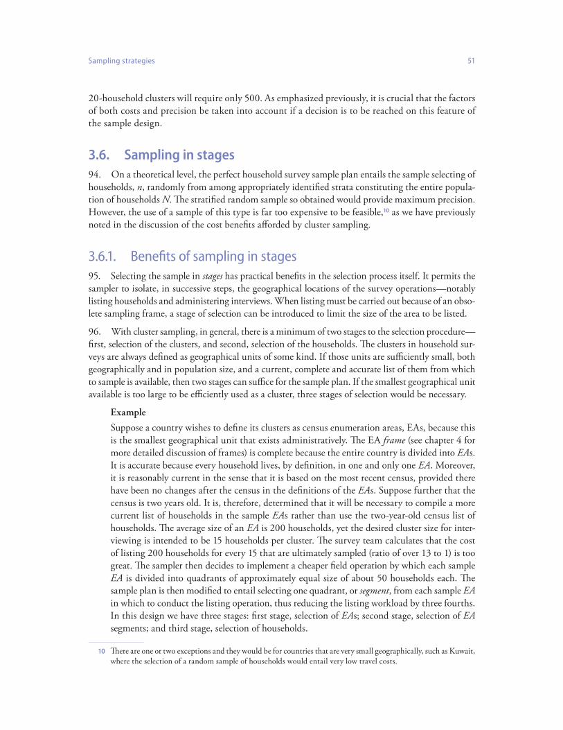
Sampling strategies 51
20‑household clusters will require only 500. As emphasized previously, it is crucial that the factors of both costs and precision be taken into account if a decision is to be reached on this feature of the sample design.
Sampling in stages3.6. On a theoretical level, the perfect household survey sample plan entails the sample selecting of 94.
households, n, randomly from among appropriately identified strata constituting the entire popula‑tion of households N. The stratified random sample so obtained would provide maximum precision. However, the use of a sample of this type is far too expensive to be feasible,10 as we have previously noted in the discussion of the cost benefits afforded by cluster sampling.
Benefits of sampling in stages3.6.1. Selecting the sample in 95. stages has practical benefits in the selection process itself. It permits the
sampler to isolate, in successive steps, the geographical locations of the survey operations—notably listing households and administering interviews. When listing must be carried out because of an obso‑lete sampling frame, a stage of selection can be introduced to limit the size of the area to be listed.
With cluster sampling, in general, there is a minimum of two stages to the selection procedure—96. first, selection of the clusters, and second, selection of the households. The clusters in household sur‑veys are always defined as geographical units of some kind. If those units are sufficiently small, both geographically and in population size, and a current, complete and accurate list of them from which to sample is available, then two stages can suffice for the sample plan. If the smallest geographical unit available is too large to be efficiently used as a cluster, three stages of selection would be necessary.
Example
Suppose a country wishes to define its clusters as census enumeration areas, EAs, because this is the smallest geographical unit that exists administratively. The EA frame (see chapter 4 for more detailed discussion of frames) is complete because the entire country is divided into EAs. It is accurate because every household lives, by definition, in one and only one EA. Moreover, it is reasonably current in the sense that it is based on the most recent census, provided there have been no changes after the census in the definitions of the EAs. Suppose further that the census is two years old. It is, therefore, determined that it will be necessary to compile a more current list of households in the sample EAs rather than use the two‑year‑old census list of households. The average size of an EA is 200 households, yet the desired cluster size for inter‑viewing is intended to be 15 households per cluster. The survey team calculates that the cost of listing 200 households for every 15 that are ultimately sampled (ratio of over 13 to 1) is too great. The sampler then decides to implement a cheaper field operation by which each sample EA is divided into quadrants of approximately equal size of about 50 households each. The sample plan is then modified to entail selecting one quadrant, or segment, from each sample EA in which to conduct the listing operation, thus reducing the listing workload by three fourths. In this design we have three stages: first stage, selection of EAs; second stage, selection of EA segments; and third stage, selection of households.
10 There are one or two exceptions and they would be for countries that are very small geographically, such as Kuwait, where the selection of a random sample of households would entail very low travel costs.

52 Designing Household Survey Samples: Practical Guidelines
Use of dummy stages3.6.2. Often, so‑called dummy stages are used in sample selection to avoid having to sample from an 97.
enormous file of units in the penultimate stage. The file may contain so many units and may be so unwieldy that it cannot be realistically managed through tedious manual selection. Even if the file is computerized, it may still be so large that it cannot be managed efficiently for sample selection.11 Dummy stages allow one to narrow down the sub‑universes to more manageable numbers by taking advantage of the hierarchic nature of administrative subdivisions of a country.
For rural surveys in Bangladesh, for example, villages are often designated as belonging in the 98. next‑to‑last stage of selection. There are more than 100,000 villages in Bangladesh, which are far too many to manage efficiently for sample selection. If a sample plan is designed to select 600 villages at the penultimate stage, for example, only 1 in about 167 would be selected in Bangladesh. To cut down on the size of the files for sample selection, it might be decided to select the sample in stages using the hierarchy of geographical units into which Bangladesh is divided—thanas, unions and villages. The sample selection would proceed in steps by first selecting 600 thanas, using probability proportionate to their sizes (this method is discussed in detail in section 3.7). Next, exactly one union would be selected from each sample thana, again using the probability proportionate to size: thus, there would be 600 unions in the sample. Third, one village would be selected using probability proportionate to size from each sample union, again resulting in 600 villages. Finally, the sample of households would be selected from each sample village. This would generally produce a systematic sample of all the households in each sample village.
The sample selection methodology described above is in effect a two‑stage sampling of vil‑99. lages and households, although two dummy stages were utilized initially for selecting the thanas and unions from which the villages were to be selected. It is necessary in this instance to illustrate the dummy character of the first two stages mathematically by examining the probabilities at each selection stage and the overall probability.
First stage of selection: thanas3.6.2.1.
Thanas are selected with probability proportionate to size. The probability at that stage is 100. given by
11 It is possible, however, a very large computer file more manageable for sampling by for example, decomposing it into separate sub‑files for each stratum or administrative area (a region or province, for example).
12 This is the measure of size and it may, instead, be the population of the thana, provided the number used is con‑sistent for all measures of size at every stage.
P amm
t
t1 = ( )
∑ , (3.11)
where P1 is the probability of selecting a given thana; a is the number of thanas to be selected (600 in this illustration); and mt is the number of rural households12 in the tth thana according to the sampling frame used (for example, the most recent population census).
The factor 101. mt∑ is the total number of rural households over all the thanas in the country. It should be noted that the actual number of thanas selected may be less than 600. This can occur whenever one or more thanas are selected twice, a possibility for any thana for which its measure of size exceeds the sampling interval. The sampling interval for selecting thanas is given by m at ÷∑ .

Sampling strategies 53
Thus, if the sampling interval is, say, 12,500 and the thana contains 13,800 households, it will auto‑matically be selected once and have a chance of 1,300/12,500 of being selected twice (the numerator is equal to 13,800‑12,500).
Second stage of selection: unions3.6.2.2.
At the second stage, one union is selected from each sample thana, again with 102. probability proportionate to size. Practically, this is accomplished by listing all the unions in the selected thana, cumulating their measures of size, mu, and choosing a random number between 1 and mt, the measure of size for the sample thana. The cumulant whose value is the smallest number equal to or greater than the random number identifies the selected union (or an equivalent convention is used to identify the selected union). If a thana was selected more than once in the first stage, the same number of unions would then be selected from it. The probability at the second stage is given by
where P2 is the probability of selecting a given union in the sample thana; (1) signifies that only one union is selected; and mu is the number of households in the uth union according to the frame.
Third stage of selection: villages3.6.2.3.
At the third stage, one village is selected with103. probability proportionate to size from each sample union with. The probability at the third stage is given as
P mm
ut2 1= ( )( ) , (3.12)
where P3 is the probability of selecting a given village in the sample union; (1) signifies that only one village is selected; and mv is the number of households in the vth village according to the frame.
Fourth stage of selection: households3.6.2.4.
At the fourth stage, we will assume that the frame list of households is available for each 104. selected village, so that the sample of households can be systematically selected from those lists. A fixed number of households is selected from each sample village; that number being the prede‑termined cluster size. The probability at the fourth stage is given as
P mm
vu3 1= ( )( ) , (3.13)
where P4 is the probability of selecting a given household in the sample village; and b is the fixed number of households selected in each village.
Overall probability of selection3.6.2.5.
The overall probability, which is the product of probabilities at each stage is given, as105.
P bmv4 = ( ) , (3.14)
P P P P P = 1 2 3 4. (3.15)

54 Designing Household Survey Samples: Practical Guidelines
Substituting, we have
Note that 106. P2 and P3 cancel out completely, demonstrating the dummy nature of the “four” stage selection process. Thus, the thanas and unions, though physically “selected”, nevertheless serve merely to pin down where the sample villages are located.
The two‑stage design3.6.3. Recently, much attention has been given to the use of two‑stage sample designs in developing 107.
countries. It is the sample design of choice for the Multiple Indicator Cluster Surveys (MICS) carried out by the United Nations Children’s Fund (UNICEF) in over 100 countries since the mid‑1990s. They are also used predominantly in the Demographic and Health Surveys (DHS).
Typically, the two‑stage design consists simply of a sample selected with probability propor‑108. tionate to size of several hundred geographical units, suitably stratified, at the first stage. A current listing of households may be developed in the first‑stage sample units, depending upon the avail‑ability of information regarding the address and/or location of the households and whether that information is current. This is followed by a systematic sample of a fixed number of households at the second stage. The geographical units, commonly referred to as the “clusters”, are usually defined as villages or census enumeration areas in rural areas and city blocks in urban areas.
The two‑stage design described above is appealing in many ways but chiefly because of its 109. simplicity. It is always advantageous in sample design to strive more towards simplicity than towards com‑plexity in order to reduce the potential for non‑sampling error in sample implementation. The two‑stage design has useful features that make it comparatively simple and desirable. For example:
As described, the sample design is self‑weighting (all the households in the sample are •selected with the same probability), or approximately self‑weighting (see secs. 3.7.1 and 3.7.2 for the distinction between samples selected with probability proportionate to size and those selected with probability proportionate to estimated size.
Clusters defined in terms of • EAs or city blocks are of a convenient size (not too big)—in most countries, especially if a fresh listing of households must be made before the final stage of selection.
EA• s, city blocks and most villages are usually mapped, either for census operations or for other purposes, with well‑delineated boundaries.
Sampling with probability proportionate to size 3.7. and with probability proportionate to estimated size
Section 3.5 presented an example where sampling with probability proportionate to size 110. featured prominently in the selection of the clusters for the sample. The present section discusses probability proportionate to size sampling in greater detail.
P am m m m m m b m
a b
t t u t v u v= ( ) ( )( ) ( )( ) = ( )
∑
1 1
(( )[ ] ∑mt (3.16)

Sampling strategies 55
Sampling with probability proportionate to size3.7.1. Use of 111. probability proportionate to size sampling permits the sampler to exercise greater con‑
trol over the ultimate sample size in cluster surveys. In situations where the clusters are all the same size, or approximately so, there would be no advantage to using probability proportionate to size sampling. Suppose, for example, every block in a particular city contained exactly 100 households and one wanted a sample of 1,000 households spread among a sample of 50 city blocks. The obvi‑ous sample plan would be to select an SRS sample of 50 blocks, that is, to say an equal‑probability sample and then systematically select exactly 1 in 5 of the households from each block (also an equal‑probability sample). The result would be a sample of precisely 20 households per block or 1,000 altogether. The selection equation in this case is
13 See (Kalton, 1983, pp. 38‑47) for the development of this notation and additional discussion on sampling with probability proportionate to size.
Where p is the probability of selecting a household; (50/M) is the probability of selecting a block; M is the total number of blocks in the city; and (1/5) is the probability of selecting a household within a given sample block.
P112. reduces to 10/M. Since M is a constant, the overall probability of selection for each sample household is equal to 10 divided by the number of blocks, M.
In real situations, however, blocks or other geographical units that might be used as clusters 113. for household surveys are seldom so unvarying in their sizes. For the example above, they may range in size from, say, 25 to 200. An equal probability sample of blocks could result in an “unlucky” selec‑tion of mostly small ones or mostly large ones. In that case, the result would be an overall sample size drastically different from the desired 1,000 households discussed in the example. One method of reducing the potential for widely variable sample sizes is to create strata based on the size of the clusters and select a sample from each stratum. That method is not generally recommended because it may reduce or complicate the use of other stratification factors in the sample design. Sampling with probability proportionate to size is the preferred solution because it permits greater control over the ultimate sample size without introducing the need for stratification by size.
To illustrate sampling, with probability proportionate to size we start with the selection equa‑114. tion mentioned above but expressed more formally for a two‑stage design13 as follows:
p M= ( )( )50 1 5 .
where P αβ( ) is the probability of selecting household β in cluster α ; P α( ) is the probability of selecting cluster α ; P β α( ) is the conditional probability of selecting household β in the second stage given that cluster α was selected at the first stage.
To fix the overall sample size in terms of number of households, we require an 115. equal‑proba‑bility sample of n households out of the population of N households. Thus, the overall sampling rate is n/N which is equal to P αβ( ) as defined below. Further, if the number of clusters to be sampled
P P Pαβ α β α( ) = ( ) ( ) , (3.17)

56 Designing Household Survey Samples: Practical Guidelines
is specified as a then ideally we need to select b households from each cluster regardless of the sizes of the selected clusters. If we define mi as the size of the ith cluster, then we need P β α( ) to be equal to b/mi. Hence,
Since n = ab, we have
P P b miαβ α( ) = ( )[ ] .
ab N P b mi= ( )[ ] α .
Solving the latter equation for P α( ), we obtain
P a m Niα( ) = ( )( ) . (3.18)
Note that 116. N mi= ∑ , so that the probability of selecting a cluster is therefore proportional to its size. The selection equation for a probability proportionate to size sample of first‑stage units in which the ultimate units are nevertheless selected with equal probability is therefore
P a m m b mi i iαβ( ) = ( )( ) ∑ (3.19)
= ( ) ∑ab mi (3.20)
The sample design so achieved is self‑weighting, as can be seen from equation (3.19), because 117. all the terms of the equation are constants; recall that, while mi is a variable, the summation, mi∑ is a constant equal to N. Figure 3.2 below provides an example of how to select a sample of clusters using probability proportionate to size.
With respect to physically selecting the sample, note that in figure 3.2, the sampling interval, 118. I, is successively added to the random start RS, seven times (or a–1 times, where a is the number of clusters to be selected). The resulting selection numbers are 311.2 (which is the RS), 878.8, 1,446.4, 2,014, 2,581.63,149.2, 3,716.8 and 4284.4. The cluster that is sampled for these eight selection numbers is, in each case, the one whose cumulated measure of size is the smallest value equal to or greater than the selection number. Thus cluster 03 is selected because 377 is the smallest cumulant equal to or greater than 311.2 and cluster 26 is selected because 3,744 is the smallest cumulant equal to or greater than 3,716.8.
Although the illustration does not conclusively demonstrate this (because only eight clusters 119. were selected), sampling with probability proportionate to size tends to select larger rather than smaller clusters. This is perhaps obvious, since from formula (3.17) it can be seen that the probability of selecting a cluster is proportionate to its size; thus, a cluster containing 200 households is twice as likely to be selected as one containing 100 households. Consequently, it should be noted that the same cluster may be selected more than once if its measure of size exceeds the sampling interval, I. However, none of the clusters in the figure fit that condition; but if this should happen, the number of households to be selected in such a cluster would be double for two “hits”, triple for three hits and so forth.

Sampling strategies 57
Figure 3.2Example of systematic selection of clusters, with probability proportionate to size
Cluster/PSU numberMeasure of size
(number of households) Cumulative Sample selection
001 215 215
002 73 288
003 89 377 311.2
004 231 608
005 120 728
006 58 786
007 99 885 878.8
008 165 1, 050
009 195 1, 245
010 202 1, 447 1,446.4
011 77 1, 524
012 59 1, 583
013 245 1, 828
014 171 1, 999
015 99 2, 098 2,014.0
016 88 2, 186
017 124 2, 310
018 78 2, 388
019 89 2, 477
020 60 2, 537
021 222 2, 759 2,581.6
022 137 2, 896
023 199 3, 095
024 210 3, 305 3,149.2
025 165 3, 470
026 274 3, 744 3,716.8
027 209 3, 953
028 230 4, 183
029 67 4, 250
030 72 4, 322 4,284.4
031 108 4, 430
032 111 4, 541
Sample instructions: Select 8 PSUs (clusters) from 32 in the universe using probability proportionate to size; selection interval (I) therefore equals 4,541/8, OR 567.6, where 4,541 is the total cumulated measure of size for all clusters and 8 is the number of clusters to be selected; random start (RS) is a random number between 0.1 and 567.6 chosen from a random number table; in this illustration, RS = 311.2.

58 Designing Household Survey Samples: Practical Guidelines
Sampling with probability proportionate to estimated size3.7.2. The 120. probability proportionate to size sampling methodology described in the previous sec‑
tion is somewhat ideal and may not be realizable in practical applications in most cases. This is because the measure of size used to establish the probability of selection of the cluster at the first stage is often not the actual measure of size when the sample of households is selected at the second stage.
In household surveys, the measure of size generally adopted for the first‑stage selection 121. of primary sampling units or clusters is the count of households (or population) from the most recent census. Even if the census is very recent, the actual number of households at the time of the survey is likely to be different, if only by a small amount. An exception occurs, however, when the second‑stage selection of households is taken directly from the same frame as the one used to establish the measures of size (for further discussion of sampling frames see chapter 4).
Example
Suppose that a household survey is conducted three months after the conclusion of the population census. Instead of making a fresh listing of households in the selected clusters, the survey team decides to use the census list of households at the second stage of a two‑stage sample because it is plausibly assumed that the census list is, for all practical purposes, cur‑rent and accurate. At the first stage, a sample of villages is selected using the census count of households as the measure of size for each village. For each sample village, the measure of size, mi, is identical to the actual number of households from which the sample is to be selected. Thus, if village A is selected and it contained 235 households according to the census, the list from which the sample of households will be selected for the survey also contains 235 households.
In many household survey applications that are based on census frames, however, the sur‑122. vey is conducted many months and sometimes years after the census was taken (see chapter 4 for further discussion updating sampling frames). Under those circumstances it is often decided to conduct a field operation in order to prepare a fresh list of households in clusters that are selected for inclusion in the sample at the first stage. From the fresh listing, a sample of households is then selected for the survey.
The measure of size, 123. mi, used to select the cluster is the census count of households discussed in the example above. However, the actual list from which the sample of households is selected will be different. It will of course have a different measure of size to some degree depending upon the length of time between the taking of the census and the preparation of the survey listing. Dif‑ferences will occur because of migration into and out of the cluster, construction of new or demo‑lition of old housing, establishment of separate households when marriage occurs (sometimes within the same dwelling unit of the parental household) and death. When the sample is selected with probability proportionate to estimated size, its probability from the selection equation is
P a m m b mi i iαβ( ) = ( )( ) ∑ ’ , (3.21)
where mi’ is the count of households according to the listing operation and the other terms are defined as previously.

Sampling strategies 59
Since 124. mi’ and mi are likely to be different for most, if not all sample clusters, calculation of the probability of selection (and hence the weight, that is, to say, the inverse of the probability) should take the difference into account. As equation 3.20 shows, each cluster would have a different weight, thus precluding a self‑weighting sample design.
By using the exact weights that compensate for differences between census and survey meas‑125. ures of size, the resulting survey estimates will be unbiased. Failure to adjust the weights accord‑ingly produces biased estimates whose magnitudes undoubtedly increase as the interval between the census and the survey lengthens. It should be noted, however, that when there are minor differences between mi’ and mi, the sample is virtually self‑weighting; and it may, under some circumstances,14 be prudent to generate the survey estimates without weighting, since the biases would be negligible. Before this course of action is decided upon, however, it would be essential to examine mi’ and mi
cluster by cluster to assess empirically whether the differences are minor.
There is an alternative strategy that may be used to select households at the last stage whenever 126. sampling with probability proportionate estimated size is employed—one in which the sample is actually self‑weighting. It involves selecting households at a variable rate within each cluster depend‑ing upon its actual size (this is discussed in the next section).
Options in sampling3.8. The present section discusses some of the many options that may be considered in designing 127.
an appropriate sample for a general‑purpose household survey, focusing primarily on strategies at the penultimate and final stages of selection since those are the stages at which several alternatives are available. It examines the choice of equal‑probability or probability proportionate to size sampling of clusters at the penultimate stage together with fixed‑rate versus fixed‑size sampling of households in the final stage and, to some extent, summarizes prior sections with respect to issues of control‑ling sample size, and self‑weighting versus non‑self‑weighting designs, as well as other issues such as interviewer workloads. In addition, it reviews particular designs that are currently being widely used such as those for the Demographic and Health Survey and the UNICEF mid‑decade multiple Indicator Cluster Survey. Those designs provide additional options that merit consideration, includ‑ing the use of compact (take‑all) and non‑compact clusters.
Equal‑probability sampling, sampling with probability 3.8.1. proportionate to size, fixed‑size and fixed‑rate sampling
In table 3.4, potential designs provide a framework for discussing the procedures, conditions, 128. advantages and limitations of various sample plans.
We have discussed how probability proportionate to size sampling of primary sampling units 129. or clusters is a means of controlling the ultimate sample size more accurately than equal‑probability sampling, which is its chief advantage, especially if the clusters are widely variable in the number of households each contains. Control of the sample size is important not only for its cost implications
14 In surveys where the estimates are restricted to proportions, rates or ratios this would be an appropriate strategy; for surveys where estimated totals or absolutes are desired weighting must be used irrespective of whether the sample is self‑weighting, approximately self‑weighting or non‑self‑weighting.

60 Designing Household Survey Samples: Practical Guidelines
but also for permitting the survey manager to accurately plan interviewer workloads in advance of survey operations. Equal‑probability sample selection, on the other hand, is simpler to carry out than probability proportionate to size sampling and makes sense when the measures of size (MOS), of the clusters are approximately equal or vary little. As a practical matter, sampling with probability proportionate to estimated size must be used in lieu of sampling with probability proportionate to size whenever the actual measure of size is different from that given in the frame.
Selection of a fixed number of households in each sample cluster has two very important 130. advantages: first, the sample size is controlled precisely; and second, the method provides the means for the survey manager to assign exact workloads to interviewers and to equalize those workloads if he or she so chooses. Fixed‑size sampling, however, is somewhat complicated, as it requires the calculation of different sampling intervals for each cluster. Applying different sampling intervals can be confusing and is error‑prone. There is, however, a built‑in quality control check, since the number of households to be selected is known in advance. Still, the complications can result in inefficiency arising from the time lost through having to correct errors in selection.
Fixed‑size sampling requires, by definition, a listing of households based upon which the 131. selected households can be designated and identified. Most often, the listing is a current one having been prepared as part of pre‑survey field operations. It is useful to ensure that selection of the sample households is carried out in a central office and that it is undertaken by someone other than the lister himself so as to minimize the possibility of bias in the selection procedure.
Alternatively, households may be sampled at a fixed rate in every cluster. In this case, selec‑132. tion is simpler and less error‑prone. An advantage in the field is that the sampling can be done at the time the interviewer is canvassing the cluster to obtain a current listing of households. This is accomplished by designing the listing form to show predesignated lines for identifying the sample households. That the listing and sampling can be carried out in a single visit has obvious advantages in terms of cost; however, there are some important limitations.
One limitation of fixed‑rate sampling is that it exerts little control over the sample size or the 133. interviewer workloads, unless the measure of size for each cluster is approximately the same. Another, more serious limitation is that when interviewers are entrusted with actually selecting the households for the sample, that is, to say identifying the ones that are to be listed on the sample lines, biased selection often results. Countless studies have been conducted demonstrating that the households that are selected when the interviewers are in control tend to be smaller in size, suggesting that interviewers may consciously or unconsciously choose households that have fewer respondents in order to decrease the workload.
A design is self‑weighting or not depending upon the particular mix of sampling procedures 134. at each stage. Thus, a two‑stage design comprising sampling of clusters with probability proportionate
Table 3.4Alternative sample plans: last two stages of selection
Selection of penultimate unitsFixed cluster size (number of households)
Fixed rate of selection in each cluster
Probability Proportionate to size Plan 1 Plan 2 [not recommended]
Probability proportionate to estimated size Plan 3 Plan 4 [not recommended]
Equal‑probability Plan 5 Plan 6

Sampling strategies 61
to size and fixed‑size sampling of households is self‑weighting while the combination of probability proportionate to size and fixed‑rate is not. The discussion that follows indicates which of the plans in table 3.4 are self‑weighting.
Plan 1: probability proportionate to size, fixed cluster size3.8.1.1.
ConditionsVariable MOS for universe of clusters•Households selected from same lists (example: census list of households) that are used •for MOS
AdvantagesControl of total sample size and hence of cost•Control of interviewer workloads•Self‑weighting•
LimitationsSampling with probability proportionate to size • somewhat more difficult to apply than equal probability samplingDifferent selection rates for choosing households from each cluster, with potential for errors•
Plan 2: probability proportionate to size, fixed rate3.8.1.2.
There are no plausible conditions under which this design would be used. If the clusters are 135. variable in size, then sampling with probability proportionate to size together with a fixed cluster size is the proper plan to use. If clusters are of approximately equal size, then fixed‑rate sampling is appropriate but the clusters themselves should be selected using equal‑probability sampling.
Plan 3: probability proportionate to estimated size, fixed cluster size3.8.1.3.
ConditionsVariable • MOS for universe of clustersHouseholds selected from fresh listings updating those from the frame to establish the •original MOS
AdvantagesControl of total sample size and hence of cost•Control of interviewer workloads•More accurate than probability proportionate to size for a given frame because the house‑•hold listings are current
LimitationsProbability proportionate to estimated size somewhat more difficult to apply than •equal‑probability sample selection methodDifferent selection rates for choosing households from each cluster with potential for •errorsNot self‑weighting•
Plan 4: equal‑probability, fixed rate3.8.1.4.
There are no plausible conditions for utilizing plan 4 for the reasons stated above for plan 2.136.

62 Designing Household Survey Samples: Practical Guidelines
Plan 5: equal‑probability, fixed cluster size3.8.1.5.
ConditionsMOS• for universe of clusters are approximately equal or minimally variable
AdvantagesControl of total sample size (but somewhat less than that of plan 1) and hence of cost•Control of interviewer workloads but again somewhat less than that of plan 1•Equal‑probability• easier to apply than probability proportionate to size or probability proportionate to estimated size
LimitationsDifferent selection rates for choosing households from each cluster with potential for •errorsNot self‑weighting•
Plan 6: equal‑probability, fixed rate3.8.1.6.
ConditionsMOS for universe of clusters are virtually equal•
AdvantagesSelf‑weighting•Very simple to select sample at both stages•
LimitationsPoor control of total sample size, with cost and reliability consequences, especially if cur‑•rent MOS is substantially different from frame MOS, and reliability consequences if sam‑ple is much smaller than targetedLittle control of interviewer workloads•
Demographic and Health Survey (DHS)3.8.2. While the focus of the Demographic and Health Survey (DHS) is women of child‑bearing 137.
age, its sample design is appropriate for general‑purpose surveys.
The Demographic and Health Survey, which has been widely applied in scores of develop‑138. ing countries since 1984, promotes the use of the standard segment design,15 for its convenience and practicality, in its sampling manual. A standard segment is defined in terms of its size, usually 500 persons. Each geographical area unit of the country that belongs to the sampling frame is assigned a measure of size calculated as its population divided by 500 (or whatever standard segment size is decided upon for the country in question). The result, rounded to the nearest integer, is the number of standard segments in the area unit.
A probability proportionate to size sample of area units is selected using the number of stand‑139. ard segments as the measure of size. Since the area units that are used for this stage of the sample
15 The standard segment design was also used in the Pan‑Arab Project for Child Development (PAPCHILD) survey programme of the 1980s‑1990s—see League of Arab States (1990).

Sampling strategies 63
are, typically, enumeration areas (EAs), city blocks or villages, the MOS for a large proportion of them is equal to one or two. For any selected area unit with an MOS greater than one, a mapping operation is organized in which geographical segments are created, the number of such segments equalling the MOS. Thus, a sample area unit with MOS of 3 will be mapped so as to divide the unit into three segments of roughly equal size, to the extent that natural boundaries will allow, in terms of the number of persons in each segment (as opposed to its geographical size).
Each area unit with 140. MOS of 1 is automatically in the sample and in each of the others, one segment is selected at random by equal‑probability sampling. All sample segments, including those automatically chosen, are then canvassed to obtain a current listing of households. A fixed frac‑tion (rate) of households is selected systematically from each sample “cluster” for the DHS inter‑view. Because the segments are all of approximately the same size, the sampling procedure yields a two‑stage equal‑probability sampling sample of segments and of households.
The DHS standard segment design is close to plan that of 6 above: equal‑probability141. selec‑tion of clusters and fixed‑rate selection of households within sample clusters (also equal‑probability). However, through its standard segmentation procedure it avoids the serious limitations noted above for plan 6: the overall sample size is controlled almost precisely as well as interviewer workloads.
An important advantage of the standard segment design is that the listing workload at the 142. penultimate stage of selection is substantially reduced. For every area unit consisting of s segments, the listing workload is reduced to 1/s (when there is only one segment, there is no reduction). For example, if a given area unit contains four segments, the listing workload is only one fourth what it would be if listing had to be carried out in the entire area. Sample preparation costs are thus reduced because of this feature.
While listing costs are lower, the reduction comes at an additional price. A limitation of the 143. standard segment design is that mapping operations must be conducted for segments with a MOS greater than 1. Mapping can be tedious and costly, requires careful training and is subject to errors. The fact that, often, natural boundaries are not well defined hinders a reasonable delineation of seg‑ments within the area unit. That deficiency makes it difficult for interviewers who visit the segment later to locate exactly where the selected household might be. The latter problem can be ameliorated somewhat, however, by including the name of the head of the household at the listing stage, in which case poorly drawn boundaries are less troublesome.
Modified cluster design: Multiple Indicator 3.8.3. Cluster Surveys (MICS)
Survey practitioners commonly complain of the expense and time required to list households 144. in the sample clusters that are selected in the penultimate stage. Listing is generally required in most surveys—including, as mentioned, the standard segment design method of DHS—in order to obtain a current list of households from which to select those for the survey interview. This is especially crucial when the sampling frame is more than a year old. The listing operation encompasses a significant survey cost and process that are often overlooked in both budgetary planning and survey scheduling. A visit to the field separate from that required to conduct the survey interviews, must be made to effectuate listing. Moreover, it is frequently the case that the ratio of households to be listed is as much as 5‑10 times the number to be selected. For example, suppose the sample plan is to select 300 PSUs with

64 Designing Household Survey Samples: Practical Guidelines
cluster sizes of 25 households for a total of 7,500 to be interviewed. If the average penultimate PSU contains 150 households, then 45,000 households must be listed.
The sampling strategy used for the Expanded Programme on Immunization (EPI) Cluster Sur‑145. vey (World Health Organization, 1991) was developed by the Centers for Disease Control and the World Health Organization (WHO) partly to avoid the expense and time involved in listing. The EPI Cluster Survey which is intended to estimate immunization coverage of children, has been widely used in scores of developing nations for more than two decades. An important statistical issue (Turner, Mag‑nani and Shuaib, 1996) concerns the sampling methodology. The cluster survey methodology utilizes a quota sample at the second stage of selection, even though the first‑stage units (villages or neighbor‑hoods) are usually selected in accordance with the tenets of probability sampling. The quota sample method that is often used, although there are variations, entails commencing the survey interviewing at some central point in the selected village and then to proceed in a randomly determined direction, while continuing to interview households until a particular quota is met. Under the EPI Cluster Sur‑vey variation, households continue to be visited until seven children in the target age group are found. While there is no intentional bias with the utilization of these kinds of techniques, various criticisms have been registered by many statisticians over a long period of time, including Kalton (1987), Scott (1993) and Bennett (1993). The chief criticism is that the methodology does not produce a probability sample (see section 3.2 on probability sampling versus other sampling methods for a discussion on why probability sampling is the recommended approach in household surveys).
A variation of the EPI Cluster Survey method, the so‑called modified cluster survey (MCS) 146. design, was developed in response to the need for a sampling strategy that avoided listing operations but was nevertheless grounded in probability sampling. Various applications of the MCS design, as well as other designs, have been carried out around the globe in the Multiple Indicator Cluster Sur‑veys (MICS) sponsored by UNICEF to monitor certain goals and targets of the World Summit for Children relating to the situation of children and women (United Nations International Children’s Education Fund, 2000).
The MCS design is a minimalist sampling strategy. It uses a simple two‑stage design, employ‑147. ing careful stratification plus quick canvassing and area segmentation. There is no listing operation. Essential features of the MCS sample design are:
Selection of a first‑stage sample of area units such as villages or urban blocks using • prob‑ability proportionate to size or equal‑probability depending upon how variable the PSUs are with respect to their measures of size. Old measures of size can be used even if the census frame is a few years old, although the frame must fully cover the population of interest, whether national or localized.
Visits to each sample area unit for quick canvassing plus area segmentation using existing •maps or sketch maps, with the number of segments being predetermined and equal to the census measure of size divided by the desired (expected) cluster size. The segments that are created are approximately equal in population size.
Selection of one area segment with equal probability from each sample PSU.•
Conduct of interviews with all the households in each selected segment.•
Use of segmentation without listing is the key advantage of the Measure of Size design. 148. This differs from the standard segment design of Demographic Health Survey which requires each segment to be listed. The segmentation operation also partially compensates for using a frame that

Sampling strategies 65
may be out of date. While this has the advantage of producing an unbiased estimate, it also has the limitation of these being less control over the ultimate sample size because a segment selected could, owing to growth, have a much larger size than that indicated by the frame.
Mapping, however, is required for the Measures of size design just as it is for the standard seg‑149. ment design of the Demographic Health Survey, with all the limitations, that this entails, as mentioned for the DHS method. In addition, the creation of small segments, whose size is the cluster size, that are accurately delineated can be difficult when natural boundaries are non‑existent for small areas. There is a final limitation: in as much as the segment interviewed is a compact cluster—all the households are geographically contiguous—this has a bigger design effect, because of the relatively high intra‑class correlation, than that produced with the non‑compact clusters of the standard segment design.
Special topics: two‑phase samples and sampling for trends3.9. The present section covers two special topics on sample design in household surveys: 150.
(a) two‑phase sampling, in which the first phase is used for a short interview in order to screen the household residents for persons who belong to the target population and the second phase entails selection of a sample of those who fit the criteria; and (b) the sampling methodology whereby a survey is repeated for the purpose of estimating change or trend.
Two‑phase sampling3.9.1. A special type of sample design is needed in household surveys in case where insufficient 151.
information is available to efficiently select a sample of the target population of interest. This need arises generally when the survey target population is a subpopulation—often a rare one—whose members are present in only a small proportion of households. Examples would be members of a particular ethnic group, orphans and persons with income above or below a specified level. Careful stratification can often be used to identify, for example, area units where an ethnic group of inter‑est or high‑income persons are concentrated; but when such groups are dispersed fairly randomly throughout the population or when the target group—like orphans—is rare, then stratification is an insufficient strategy and other techniques must be used for sampling them.
One technique often used is two‑phase sampling, also referred to as post‑stratified sampling 152. or double sampling. It involves four steps:
(a) Selection of a “large” sample of households;
(b) Conducting a short screening interview to identify households where members of the target population reside;
(c) Post‑stratifying the large sample into two categories based upon the screening interview;
(d) Selection of a subsample of households from each of the two strata for a second, longer interview with the target group.
The objective of the two‑phase approach is to save on costs by having a short screening inter‑153. view in the initial, large sample. It is followed by the more extensive interview at a later date, but only in the qualifying households. For that reason, the initial sample is often one that was chosen for another purpose and the screening interview is appended as a “rider” to the parent survey. The procedure thus allows most resources to be allocated to the second‑phase sampling and interviewing with only a modest budget required for the screening phase.

66 Designing Household Survey Samples: Practical Guidelines
Example
Suppose that a survey is being planned of 800 orphaned children who reside in households of surviving parents or other relatives (as opposed to orphans living in institutional settings). Suppose further that it is estimated that 16,000 households would have to be sampled to locate 800 orphans—about 1 orphan in every 20 households. Because the expense of designing and administering a sample of 16,000 households is considered impractical for only 800 detailed interviews, it is decided to make use of a general‑purpose survey on health that is also being planned. The health survey is designed for a sample of 20,000 households. The survey managers of the two surveys agree that a rider will be appended to the health survey consisting of a single question, Is there anyone aged 17 years or under living in this household whose mother, father or both have died? The rider question would be expected to identify households containing about 1,000 orphans. The orphan survey manager would then plan to subsample 80 per cent of those households for the detailed interview.
The example above also serves to illustrate 154. when two‑phase sampling is an appropriate strat‑egy. Note that the targeted sample size in the illustration is only 800 orphans but the sample size in terms of the number of households necessary to find that many orphans is 16,000. Thus, in cal‑culating the latter (see formula 3.7), the sampling technician and the survey manager would likely conclude that two‑phase sampling is the most practical and cost‑efficient design to use.
Post‑stratification of the first‑phase sample is important for two reasons. The screening ques‑155. tion or questions will almost always be brief because they are appended to another survey which undoubtedly already features a lengthy interview. The survey manager of the parent survey is unlikely to agree to a very detailed set of screening questions. Hence, it is likely that some households in the above example for which orphans were identified will have no orphans and conversely. Such misclas‑sification errors suggest that two strata should be set up, one for households where the screener result was positive and the other where it was negative. Samples would be taken from each stratum for the full interview on the grounds that misclassification probably occurred to some degree. The sample rate in the “yes” stratum would be very high—up to 100 per cent—while a much smaller fraction would be taken in the “no” stratum.
Sampling to estimate change or trend3.9.2. In many countries, household surveys are designed with the dual purpose of estimating 156.
(a) baseline indicators (their levels) on the occasion of the survey’s first being administered and (b) change in those indicators in second and subsequent administering of the survey. When the survey is repeated more than once, trends in indicators are also measured. With repeat surveying, there are various effects on sample design that are not introduced when a one‑time cross‑sectional survey is conducted. In particular, the issues that are of concern are reliability for estimating change and the proper mix in respect of using the same or different households from one occasion to the next. Related to the latter point is concern about biases and respondent burden when the same households are interviewed repeatedly.
Examination of the reliability issue, also requires a mathematical demonstration. We start 157. by looking at the variance of the estimated change, d = p1 – p2, expressed as:
σ σ σ σ σ σ ρσ σd p p p p p p p p2
12
22
1 2 12
22
1 22 2= + − = + −, , (3.22)

Sampling strategies 67
where the p value is the proportion being estimated; σd2 is the variance of the difference; σ p
2 is the variance of p on the first or second occasion, denoted by 1 or 2; σ p p1 2, is the covariance between p1 and p2; and ρ is the correlation between the observed values of p1 and p2 on the two occasions of the survey.
Whenever the estimated change is comparatively small, which is often the case, we have
Using a typical value for deff of 2.0, formula 3.19 yields:
σ σp p12
22≈ .
σ σ ρd p2 22 1= −( ). (3.23)
s pq f n or pq f nd2 2 0 2 0 4= ( ) ( ) ( ). , . . (3.24)
s pq f n or pq f nd2 2 0 7 1 4= ( ) ( ) ( ). , . . (3.25)
s pq f nd2 2= ( ) . (3.26)
Then, σ σ ρσd p p2 2 22 2= − (we can drop subscripts, 1 and 2). Hence:
To evaluate equation (3.22), we note that an estimate of 158. σ p2 for a cluster survey is that of
a simple random sample, SRS, times the sample design effect, deff. The correlation, ρ , which is highest when the same sample of households is used, may be 0.8 or even higher. In that case, the estimator, sd2, of σd
2 is given as:
If the same clusters are used but different households, 159. ρ is still positive but substantially smaller—perhaps on the order of 0.25 to 0.35. We would then have (for ρ of 0.3):
Finally, with a completely independent sample on the second occasion, using different clusters 160. and different households, ρ is zero and we have:
s pq nd2 4= ( ) . (3.27)
For repeat surveys using partial overlap, for example 50 per cent of the same clusters/house‑161. holds and 50 per cent new ones, ρ must be multiplied by a factor F equal to the proportion of the sample that overlaps. In that case, equation 3.16 becomes:
σ σ ρd p F2 22 1= −( ). (3.28)
Interesting points can be made on the above. First, the estimated variance of a comparatively 162. small estimated change between two surveys using the same sample of households is only about 40 per cent of the variance of level, on either the first or the second occasion. Using the same clusters

68 Designing Household Survey Samples: Practical Guidelines
but different households produces a variance estimate on change that is 40 per cent higher than that for level. Independent samples produce an estimated variance that is double that of level.
Thus, there are powerful advantages to using the same households in repeat surveys in terms 163. of reliability. Failing that, there are still very significant improvements to be achieved in using either (a) a portion of the same households or (b) the same clusters but with different households. Both strategies produce estimates with smaller variance compared with that for the least attractive option of using completely independent samples.
Regarding the issue of non‑sampling error, there are more occurrences of two negative 164. respondent effects—non‑response and conditioned response—the more there is repeated use of the same sample of households. Not only respondents become increasingly reluctant to cooperate, thereby increasing non‑response in later survey rounds, but they are also affected by conditioning, so that the quality or accuracy of their responses may deteriorate with repeat interviews.
Associated with conditioning is the phenomenon known as “time‑in‑sample” bias, where the 165. survey estimates from respondents reporting for the same time period but with different levels of exposure to a survey have different expected values. This phenomenon has been extensively studied and has been shown to exist for surveys on many topics—labour force, expenditures, income and crime victimization. In the United States of America, for example, where the labour‑force survey respondents are interviewed eight times, the estimate for unemployment for first‑time‑in‑sample respondents is consistently about seven per cent higher than respondents averaged over the entire eight interviews. This pattern has persisted over a number of years in the United States. To account for this bias, experts have proposed, inter alia, that:
Interviewers may not provide the same stimulus to the respondent in later interviews as •in the first one.
Respondents may learn that some responses trigger additional questions, so they avoid •giving certain answers.
The first interview may include events outside the reference period, whereas in later inter‑•views the event is “bounded”.
Respondents may actually change their behaviour because of the survey.•
Respondents may not be as diligent in providing accurate responses in later interviews once •they become bored with the survey process (Kasprzyk, 1989).
It should be noted that most of the reasons cited above apply to repeat interviews for the same 166. survey; but when the same households are used for different surveys some of the same respondent behaviour occurs.
From the above, it can be seen that there are competing effects associated with using:167.
(a) The same sample of households on each occasion;
(b) Replacement households for part of the sample;
(c) A new sample of households each time the survey is administered.
Proceeding from (168. a) to (c), sampling error on estimates of change increases while non‑sampling error tends to decrease. Sampling error is least when the same sample households are used on each occa‑

Sampling strategies 69
sion because the correlation between observations is highest. By contrast, use of the same households increases non‑sampling bias. The opposite occurs when a new sample of households is used each time.
It is option (169. b) that is generally viewed as offering a compromise in terms of balancing sam‑pling error and non‑sampling bias. If part of the sample is retained year‑to‑year, sampling error is improved over (c) and non‑sampling error is improved over (a). When a survey is conducted on only two occasions, (a) is likely to be the best option. The respondent effects are not likely to have too damaging an impact on the total survey error when a sample is used only twice. Repeat‑surveying three or more times would be better served by option (b), however. A convenient strategy is to replace 50 per cent of the sample on each occasion in a rotating pattern (see chapter 4 for examples of rota‑tion sampling in master samples).
When implementation goes wrong3.10. The present section provides a summary of actions to be taken when implementation of the 170.
sample plan encounters obstacles, most of which have already been discussed or alluded to above. However, one of the important principles stressed in this chapter and the next is that by very careful planning at the time when the sample design is conceived, many of the implementation obstacles can be forestalled. Still, unforeseen problems can arise despite the best planning.
Target population definition and coverage3.10.1. Problems often occur, for any of a variety of reasons, when the actual population covered by 171.
the survey is not the intended target population.
Example
Consider a survey intended to cover the typical target population of all people in a country. The actual population covered (that is, from which the sample is selected) is often less than the total for any of the following reasons:
Persons living in institutional quarters such as hospitals, prisons and military barracks are •not sampled.
Persons residing in certain geographical areas may be purposely excluded from coverage. •Those areas might include inaccessible terrain, areas affected by natural disasters, those declared off limits due to civil disorder or war, compounds or camps where refugees and other foreign workers reside, and so forth.
Persons who do not have permanent living arrangements are ruled as being “out of scope” for •the survey. These may include nomadic populations, boat people, transient workers, etc.
The problem regarding such subpopulations with respect to the sample plan is that they are 172. not usually identified in advance of the survey as groups that ought to be excluded. Implementation thus suffers when sample selection, by chance, chooses, say (a) a cluster that turns out to be a work camp, prison or dormitory instead of a “traditional” residential area, or (b) a PSU that is in moun‑tainous terrain and is thought to be inaccessible. The “solution” often taken in such situations is to substitute another PSU. This solution, however, entails a biased procedure.
The acceptable solution is to avoid the problem at the design phase of the sample. This is achieved 173. by first carefully defining the target population and specifying not only which subpopulations it includes

70 Designing Household Survey Samples: Practical Guidelines
but which ones are to be excluded from coverage. Second, the sample frame should then be modified to delete any geographical areas that are not to be covered by the survey. This applies as well to any special‑purpose EA—for example, a work camp—that should be excluded. Third, the sample should be selected from the modified frame. Chapter 4 discusses sampling frames in greater detail.
It should also be borne in mind that the solution suggested above serves to define the target 174. population more precisely. It is important that the exact target population be described in the survey reports so that the user is properly informed.
Sample size too large for survey budget3.10.2. Another problem occurs when the calculated sample size is larger than what the survey budget 175.
can support. When this occurs, the survey team must either seek additional funds for the survey or modify its measurement objectives by reducing either the precision requirements or the number of domains.
One way of reducing the precision (increasing the sampling error) so as to lower the cost 176. substantially is to select fewer PSUs yet retain the overall sample size. For example, instead of 600 PSUs of 15 households each (n = 9,000), the sample plan could be modified to select 400 PSUs of 22 or 23 households each (n ≈ 9,000). As for domains, one solution might be to settle upon 4 major regions of the country instead of, say, 10 provinces.
Cluster size larger or smaller than expected3.10.3. A problem that frequently occurs is that a sample cluster may be much larger than its measure 177.
of size, as a result, for example, of new housing construction, especially if the sample frame is old. The survey team may expect 125 households in a given cluster but may find 400 instead at the listing stage. A plausible solution in this case is to subdivide the cluster into geographical subsegments of approximately equal size in terms of population. The number of segments should be equal to the cur‑rent count of households divided by the original measure of size, rounded to the nearest integer. In our example, this would be 400/125 or 3.2, rounded to 3 segments. The segments would be created through mapping and quick‑counting of dwellings (as opposed to households). Then, one segment would be selected at random for listing.
The opposite problem may also occur. A cluster may be much smaller than expected, owing 178. to demolition, natural disaster or other reasons. There is often the temptation to substitute another cluster in such cases, but to do so is introducing bias. Instead, the smaller cluster should be taken as it stands. While this may result in an ultimate sample size that is smaller than that of the target, the increase in sampling error will be minor unless a large number of such clusters are involved. Taking the smaller cluster without modification (or substitution) will nevertheless allow an unbiased estimate to be produced, because the cluster “represents” the current population change that has occurred since the frame was established.
Handling non‑response cases3.10.4. Though it pertains more to survey implementation than to sample implementation, 179.
non‑response is a serious issue that can ruin household survey estimates (see chapters 6 and 8 for detailed discussion on non‑response). If non‑response is allowed to occur in more than 10‑15 per cent

Sampling strategies 71
of the sample cases, the resulting bias in the estimates may make them highly questionable. Again, a tendency in many countries is to “solve” the problem of non‑response by substituting households that do respond. The technique itself is biased because the substituted households still represent only responding households, not non‑responding ones. The characteristics of the latter two groups are known to be different with respect to important survey variables, especially those related to socio‑economic status. The preferred solution, which, unfortunately is never 100 per cent successful, is to obtain responses from initially non‑responding households. This must be done by planning, at the outset, to return to households non‑respondents in a series of successive callbacks in the effort to gain their cooperation (for refusals) or to find them at home (for absentees or the otherwise unavail‑able). As many as five callbacks may be necessary, but the minimum number should be three.
Summary guidelines3.11. This present section summarizes the main guidelines to be extracted from this chapter. While 180.
some of the guidelines would pertain under almost any circumstances (for example, “use probability sampling”), there are others for which exceptions would be appropriate, depending upon a coun‑try’s special circumstances, resources and requirements. For that reason, the guidelines, in checklist format, are presented more in the spirit of “rules of thumb” rather than as fixed and unwavering recommendations. Those involved in the survey should undertake to:
Use probability sampling techniques at every stage of selection.•
Strive as much as possible in sample design for simplicity, as opposed to complexity.•
Seek selection techniques that yield self‑weighting, or approximately self‑weighting, sam‑•ples within domains—or overall, if the design does not include domains.
Use two‑stage sample design if possible.•
Calculate sample size using formula like (3.5), adjusting the value of fixed parameters (such •as expected non‑response rate and average household size) as necessary to reflect country situation.
Use a design effect value of 2.0 as default in sample size formula unless better information •is available for the country.
Base sample size on the key estimate thought to encompass the smallest percentage of •population from among all the key estimates the survey will cover.
Budget permitting, choose margin of error, or precision level, for key estimate (above) that •is 10 per cent of the estimate, that is to say, 10 per cent relative error, at 95 per cent level of confidence; otherwise, settle for 12‑15 per cent relative error.
Define first‑stage selection units (PSUs) as census enumeration areas, EAs, if convenient •and appropriate.
Utilize implicit stratification coupled with systematic • pps sampling with probability pro‑portionate to size whenever possible, especially for multi‑purpose designs.
Limit number of estimation domains to as few as absolutely necessary (so as to bring the •sample size to a manageable level).

72 Designing Household Survey Samples: Practical Guidelines
Strive for a large number—several hundred—of clusters (or of PSUs if two stages): the •more the better.
Use small cluster sizes: 10‑15 households: the smaller the better.•
Use a constant cluster size rather than a variable one, that is to say a, fixed number of •households instead of a fixed rate.
For domains, aim towards a minimum of 50 PSUs each.•
Plan on a minimum of three, but preferably five, callbacks to convert non‑response house‑•holds.
For rare populations, consider the two‑phase sampling approach of attaching a “rider” •question onto an existing large survey already planned so as to locate the target persons; and follow up with an intensive interview on a subsample.
For surveys designed to measure change, interview the same households on both occasions •if only two interviews are to be taken; if three or more interviews are to be taken, use a scheme of partial overlap by rotating new households into the sample on each occasion.
References and further reading
Bennett, S. (1993), The EPI cluster sampling method: a critical appraisal. Invited paper, International Statistical Institute Session, Florence, Italy.
Cochran, W. (1977), Sampling Techniques, 3rd ed., New York: Wiley.
Hansen, M., W. Hurwitz and W. Madow (1953). Sample Survey Methods and Theory, New York: Wiley.
Hussmans, R., F. Mehran and V. Verma (1990). Surveys of Economically Active Population, Employment, Unemployment and Underemploymen: An ILO Manual on Concepts and Methods. International Labour Office, Geneva: Chapter 11, “Sample design”.
International Statistical Institute (1975). Manual on Sample Design. World Fertility Survey Basic Documentation. Voorburg, Netherlands.
Kalton, G. (1983), Introduction to Survey Sampling. Beverly Hills, California: Sage. Publications.
________ (1987), An assessment of the WHO Simplified Cluster Sampling Method for estimating immunization coverage. Report to UNICEF, New York.
________ (1993). Sampling Rare and Elusive Populations. Department for Economic and Social Information and Policy Analysis, Statistical Division and National Household Survey Capability Programme, INT‑92‑P80‑16E. New York: United Nations.
Kasprzyk, D., and others, eds. (1989). Panel Surveys. New York: John Wiley & Sons, Chapter 1.
Kish, L. (1965), Survey Sampling, New York: Wiley.
Krewski, D., R. Platek and J.N.K. Rao, eds. (1981). Current Topics in Survey Sampling. New York: Academic Press.
Le, T., and V. Verma (1997). An Analysis of Sample Designs and Sampling Errors of the Demographic and Health Surveys, DHS Analytical Reports, No. 3. Calverton, Maryland: Macro International Inc.

Sampling strategies 73
League of Arab States (1990), Sampling Manual, Arab Maternal and Child Health Survey, Basic Documentation 5. Cairo: Pan Arab Project for Child Development (PAPCHILD).
Macro International Inc. (1996). Sampling Manual. DHS‑III Basic Documentation, No. 6. Calverton, Maryland: Macro International Inc..
Namboodiri, N., ed. (1978). Survey Sampling and Measurement. New York: Academic Press.
Raj, D. (1972). Design of Sample Surveys, New York: McGraw‑Hill.
Scott, C. (1993), Discussant comments for session on “Inexpensive Survey Methods for Developing Countries”. Invited paper, International Statistical Institute Session, Florence, Italy.
Som, R. (1966), Practical Sampling Techniques, 2nd ed., New York: Marcel Dekker, Inc.
Turner, A., R. Magnani and M. Shuaib, (1996), A not quite as quick but much cleaner alternative to the Expanded Programme on Immunization (EPI) Cluster Survey design. International Journal of Epidemiology, (Liverpool, United Kingdom) Vol. 25, No. 1.
United Nations (1984). Handbook of Household Surveys, Revised Edition. Studies in Methods, No. 31. Sales No. E.83.XVII.13.
________ (1986). sampling frames and sample designs for integrated household survey programmes, National Household Survey Capability Programm:, New York: United Nations. Department of Technical Co‑operation for Development and Statistical Office.
________ (2005). Household Sample Surveys in Developing and Transition Countries. Studies in Methods, No. 96. United Nations publication, Sales No. E.05.XVII.6.
United Nations Children’s Fund (2000), End‑Decade Multiple Indicator Survey Manual. Chapter 4; entitled “Designing and selecting the sample”, and appendix 7; entitled “Sampling details.” New York: UNICEF.
United States Bureau of the Census (1978). Current Population Survey Design and Methodology, Technical Paper 40, Washington, D.C.: Bureau of the Census.
Verma, V. (1991), Sampling Methods. Training Handbook, Tokyo: Statistical Institute for Asia and the Pacific.
Waksberg, J. (1978), Sampling methods for random digit dialing, Journal of the American Statistical Association, vol. 73, pp. 40‑46.
World Bank (1999). Core Welfare Indicators Questionnaire (CWIQ) Handbook. Washington D.C.: World Bank, chapter 4.
Health Organization (1991). Expanded Programme on Immunization, Training for Mid‑level Managers: Coverage Survey. WHO/EPI/MLM91.10. Geneva.


75
Chapter 4
Sampling frames and master samples
Sampling frames in household surveys4.1.
The preceding chapter covered, with the exception of sample frames, the multifaceted features 1. of sample design and some of the options available for sample design in household surveys. However, one of the most crucial aspects of sample design in household surveys, is its frame, a separate chapter is being devoted to this subject.
The sampling frame has significant implications for the cost and the quality of any survey, 2. household or otherwise. In household surveys, faulty sampling frames are a common source of non‑sampling error, particularly under‑coverage of important population subgroups. This chapter attempts to elaborate best practices in frame construction and usage, taking into account various stages of sampling. It is divided into two sections: the first covers general issues on frames and their development, with emphasis on multistage sample design in household surveys; the second discusses the special issues that arise when a master sample frame is to be used.
Definition4.1.1. 1 of sample frameA simple operational definition of a sampling frame is: the 3. set of source materials from which the
sample is selected. The definition also encompasses the purpose of sampling frames, namely, to provide a means for choosing the particular members of the target population that are to be interviewed in the survey. More than one set of materials may be necessary. This is generally the case in a household survey because of its multistage nature. In early stages of selection in household surveys, samples are typically drawn from geographical area frames. In last stage, samples may be selected from either an area or a list frame (see below for a discussion on area and list frames).
Sample frame and target population4.1.1.1.
An important consideration in deciding upon the appropriate frame(s) to use for household 4. surveys is the relationship between the survey target population and the unit of selection. The unit of selection determines the frame. It also determines the probability of selection at the last stage.
1 The reader is referred to chapter 3, table 3.1 for the glossary of sampling‑related terms used in both chapters 3 and 4.

76 Designing Household Survey Samples: Practical Guidelines
Example
To illustrate, in a survey whose target population is infant children, the survey team might consider two potential frames: one could be medical facilities recording births within the past 12 months; the other households whose occupants include infants under 12 months of age. In the first instance the frame would comprise two parts, one for each stage of selection: first, the list of hospitals and clinics where infants are born; second, the list of all infants born in those facilities in the past 12 months. The units of selection would be the medical facilities at the first stage and infants at the second stage. Thus, the unit of selection and the target population are synonymous terms at the final selection stage. In the second instance, however, the frame would likely be defined (in a latter stage of selection) as a list of households in small‑area units such as villages or city blocks. In applying the sample plan, households would be selected and screened to ascertain the presence of children 0‑12 months of age. In this case, the household would be the unit of selection upon which the probability of selection was based. Note, how‑ever, that members of the target population are not actually identified and surveyed until the households are screened for their presence. Thus, the unit of selection and the target population are different in the case of the household frame.
In household surveys—the subject of this handbook—the unit of selection as well as that around 5. which the sample design is based is the household. Yet the target population, even in a general pur‑pose survey, will differ, depending upon the measurement objectives. Except for household income and expenditure surveys, the target population will usually be a population other than that of the household itself. Examples are employment surveys where the target population is generally persons aged 10 (or 14) years or over, which thus excludes young children altogether; surveys on reproduc‑tive health of women where the target population comprises women aged 14‑49 (and often only ever‑married women in that age group) etc.
Properties of sampling frames4.1.2. As discussed above, the sampling frame must of course capture, in a statistical sense, the target 6.
population. Beyond that, a perfect sample frame is one that is complete, accurate and up to date. These are ideal properties which are unattainable in household surveys. Nevertheless, it is essential to strive for them either in constructing a frame from scratch or in using one that already exists. The quality of a frame may be assessed in terms of how well its idealized properties relate to the target popula‑tion. Recall from chapter 3 that our definition of a probability sample—one in which every member of the target population has a known, non‑zero chance of being selected—is a useful barometer for judging a frame’s quality.
Depending on the degree to which there is failure to achieve each of the ideal properties, sur‑7. vey results will be biased in various ways, but often in the direction of under estimating the target population.
Completeness4.1.2.1.
The ideal frame would be deemed complete with respect to the target population if all its mem‑8. bers (the universe) were covered by the frame. Coverage of the target population(s) is therefore an essential feature in judging whether the frame is suitable for a survey. If it is not suitable, then the survey team must assess whether it can be repaired or further developed to make it more complete.

Sampling frames and master samples 77
In the previous example, infants born at home or in other places outside medical facilities would not be covered in the survey if medical facilities were used as the sole frame for sampling. Hence, in this example, there would be significant numbers of the target population that have a zero chance of inclusion in the sample, and the condition for a probability sample is violated. As a result, an estimate of the number of infants would be understated by the facility frame. Moreover, the characteristics of infants would likely be quite different from those of infants born at home. The facility frame would therefore yield biased distributions for important indicators for the infants or their care.
Inadequate coverage is also a potential problem in household surveys. For example, a national 9. survey plan may be intended to cover the entire population through a household survey. There are, however, various subgroups such as persons living in institutions, nomadic households and boat people that do not reside in households. In such a case, coverage of the total population is obviously not attainable through the household survey. Additional frames would have to be developed to cover non‑household groups in order to give their members a non‑zero probability of being included. Failing that, the actual target population would have to be modified so that what it included could be more carefully defined. In that way, users would be clearly informed of which segments of the population had been excluded from coverage.
Accuracy4.1.2.2.
Accuracy is another important feature of sampling frames, although inaccuracies are more 10. likely to occur in frames other than those used for household surveys. A frame can be said to be accurate if each member of the target population is included once and only once. Consider a list of those business establishments employing more than 50 workers. Errors could occur if (a) any estab‑lishment on the list had 49 or fewer workers, (b) any establishment with 50+ workers was missing from the list or (c) an establishment was listed more than once (perhaps under different names).
In household surveys, it is less likely that such inaccuracies containing frames would be encoun‑11. tered. However, the could arise cases where, for example: (a) a frame consisting of a computer file of enumeration areas EAs, was missing some of its elements, (b) a list frame of households in a village was missing some of those situated on the perimeter of the village, (c) in a list frame of households in an area unit, some of the households were listed in more than one unit or (d) an old list frame of households did not include newly constructed dwellings. The last‑mentioned case, that of a frame that is not current, is discussed further below.
Missing EAs or listed households within an area unit indicates, of course, that the affected house‑12. holds have no chance of being selected for the sample. Again, this would violate one of the conditions for producing a true probability sample. Duplicate listings also violate the probability criterion unless they are taken into consideration so that the true probabilities of selection can be calculated. Unfor‑tunately, omissions and erroneous duplications of the types mentioned are often not detected. The sampling technician may therefore be unaware of the need to correct the frame before sampling from it. On the other hand, a small proportion of cases that are omissions or duplicates in a frame usually will not cause any appreciable—or even noticeable—non‑sampling bias in the survey estimates.
Current frame4.1.2.3.
Ideally, of course, a frame should be current in order for it to possess the other two properties 13. of completeness and accuracy. An obsolete frame obviously contains inaccuracies and is likely to be incomplete, especially in household surveys. The quintessential example of a frame that is out of

78 Designing Household Survey Samples: Practical Guidelines
date is a population census that is several years old. The old census will not accurately reflect new construction or demolition of dwellings, in‑or outmigrants in dwelling units, births or deaths. These deficiencies violate the requirement in, that, a probability sample that each member of the target population have a known chance of selection.
Example
Suppose the frame consists of EAs defined according to the most recent census, which is four years old and no updating of the frame has been carried out. Suppose also that numerous squatter areas have sprung up on the outskirts of the capital city in EAs that were, at the time of the census, either empty, or virtually empty, of population. The sample design would offer households living in the formerly empty EAs no chance for inclusion, thus violating the prob‑ability sample conditions. In EAs that were virtually empty, another serious problem would arise even though those EAs did not technically violate probability sampling requirements. The sample would undoubtedly be selected using probability proportionate to size with the measure of size being the census population or household count. By virtue of its having had a very small population at the time of the census, any high‑growth EA would have only a slight chance of being selected when probability proportionate to size sampling was used. As a result, the sample could have an unacceptably high sampling variance.
Area frames4.1.3. In the present section and the next, we discuss the two categories of frames that are used in 14.
sampling, whether for household surveys or for other applications. It is important to note that in a multistage design, the frame for each stage must be regarded as a separate component. The specific frame is different at each stage. The sample design for a household survey will likely use both an area frame (discussed in this section) for the early stages and a list frame (discussed in the next) for the last stage.
In household surveys, an area sampling frame comprises the geographical units of a country 15. in a hierarchic arrangement. The units are variously labelled, administratively, from one country to another but typically include such terms, in descending order, as province or county; district; tract; ward and village (rural areas) or block (urban areas). For census purposes, administrative subdivisions are further classified into such entities as crew leader areas and enumeration areas or (EAs). Often the census EA is the smallest geographical unit that is defined and delineated in a country.
For survey purposes, there are four distinct characteristics of geographical units that are impor‑16. tant for sample design:
(a) They usually cover, the entire land area of a nation;
(b) Their boundaries are well delineated;
(c) There are population figures available for them;
(d) They are mapped.
Coverage of the totality of the nation’s geographical area is important, as we have noted, 17. because it is one of the criteria for achieving a bona fide probability sample. Well‑delineated boundaries that are mapped are invaluable in sample implementation because they pin down the locations where fieldwork is to be conducted. Good boundary information also helps the

Sampling frames and master samples 79
interviewer locate the sample households that are ultimately selected for interview. Population figures are needed in sample design to assign measures of size and to calculate the probabilities of selection.
The usual starting point in development of an area frame for household surveys is a country’s 18. population census based on the four factors cited above. In addition, the EA is a conveniently sized geographical unit for selection in the latter stages of sampling (the penultimate stage in a two‑stage design). In most countries, EAs are purposely constructed to contain roughly equal numbers of households—often about 100—in order to provide comparable workloads for census‑takers.
An area frame is, paradoxically, also a 19. list—because one must begin with a list of the admin‑istrative geographical units of a population in order to proceed through the early stages of selection of a household survey sample. This requires a discussion of list frames.
List frames4.1.4. A list sampling frame is, quite simply, a frame made up of a list of the target population units. 20.
Theoretically, a list frame for household surveys exists for every country just after its census is taken. The fresh census provides, in principle, a geographically arranged listing of every household—or dwelling unit—in the country.
A newly completed census list is ideal as a household sampling frame because it is as current, 21. complete and accurate as any household list could ever be. Because of the census list’s geographical arrangement, to stratify it for proper geographical distribution of the sample is fairly simple. Hence, when there is a need to conduct a census follow‑up sample survey to obtain supplemental information or information that is more detailed than the information that the census can efficiently provide, the fresh census list is thus ideally suited for use as the list frame. It is important to recognize, however, that the new census list is available only briefly as a current frame. Obviously, the longer the interval between the census and a follow‑up survey, the less useful the census listings as the frame source.
There are other lists that, depending upon their quality, might be considered appropriate 22. sampling frames for household surveys such as civil registries, and registers of utility connections. Civil registries would be candidates for frame use in countries where careful records have been kept of its citizens and their addresses. In some instances, they may be more useful than an area‑based census frame, because the registry may likely be continuously updated. Utility—usually electricity—connections may be useful as a sampling frame whenever a country’s census is seriously obsolete, but they would, of course, have to be evaluated to assess potential problems, and their impact. An obvious problem leading to under‑coverage would be households not having access to power; another requiring sorting out would be the presence of electrical hook‑ups servicing multiple households.
Another list frame that is widely used in developed countries is a register of telephone subscrib‑23. ers. Sampling is done through random digit dialling (RDD) techniques to ensure that subscribers with unpublished telephone numbers have a proper chance of being selected. Sampling through random digit dialling is not recommended, however, in countries that have low penetration rates for telephone ownership.
In a conventional household survey, the last stage of selection is, invariably, based on a list 24. frame concept. We have discussed previously how the penultimate design stage may yield a sample of clusters in which a current listing of households is compiled. From that list, the sample households
80 Designing Household Survey Samples: Practical Guidelines
are selected. Thus, we have an area frame defining the sample clusters and a list frame defining the sample households within the clusters.
Multiple frames4.1.5. Chapter 3 discussed two‑phase sampling in household surveys. It involves the use of screen‑25.
ing techniques to identify a particular target group in the first phase, followed by a second‑phase interview of a subsample of those identified. Another sampling technique that may accomplish much the same end result involves using more than one sampling frame. Usually, this involves only two frames, for which we have a dual‑frame design; occasionally, however, three of more frames may be used (multi‑frame design). For example, a population frame which is defined as a sum of several lists, from which an independent sample is selected, in this case each subframe becomes a stratum (see discussion of stratification in section 3.4.2 of chapter 3. and in Annex I). However, the common problem with such frames is duplication.
Typical dual frame in household surveys4.1.5.1.
For simplicity of presentation, we will discuss dual‑frame designs, though the principles are 26. analogous for multi‑frame designs. In general, the methodology entails combining a general‑popula‑tion area frame with a list frame of persons known to be members of the particular target population under study. For example, consider a survey intended to study the characteristics of unemployed persons. The survey could be based on an area frame of households but might be supplemented with a list‑frame sample of currently unemployed persons who are registered with the social services minis‑try. The objective of a dual‑frame sample of this type is to build up the sample size with persons that have a very high probability of being in the target population. The approach can be a cheaper and more efficient alternative to two‑phase sampling. It is necessary to use the general‑purpose household frame to account for target population members who are not on the list. In this example they would be unemployed persons not registered with social services.
Several limitations are imposed, however, with dual‑frame designs. One is that the list frame 27. must be virtually current. If a large proportion of persons selected from the list have undergone a change in status that removes them from the target population, then use of the list frame is inef‑ficient. In our example, the fact that any unemployed person would be ineligible who has become employed by the time the survey is conducted, illustrates why the list frame must be up to date.
Another limitation is imposed by the fact that the residences of persons on the list frame will 28. likely be dispersed throughout the community, which will make it is costly to interview them owing to travel. This, of course, is in stark contrast to the area‑based household frame where the sample can be selected in clusters go as to reduce interviewing costs.
A serious issue connected with dual‑frame designs is that of duplication. Generally, persons 29. included on the list frame will also be included on the area frame. Again, in our example, unemployed persons selected from a registry are members of households. They would have a duplicate chance of selection, therefore, when both frames are used. The duplication issue can be so addressed as to adjust for it properly. This, however, has implications for the content of the survey questionnaire. In our example, each unemployed person interviewed in the household sample would have to be queried as to whether he/she is registered with the ministry on its list of unemployed. For those that respond in the affirmative, further work is necessary to match their names with the list frame, a process that is
Sampling frames and master samples 81
error‑prone and fraught with complications. When a successful match is found, the survey weight of the person affected must be changed to (1/Ph + 1/Pl) to reflect the fact that she has a probability, Ph, of being selected from the household frame and a probability, Pl, of being selected from the list frame. It is important to note that matching must be done against the entire list frame and not just against those on the frame who happened to have been selected in the sample. This is because the probability (and weight) is a function of the chance of selection irrespective of whether actual selection occurs.
Multiple frames for different types of living quarters4.1.5.2.
Another type of dual‑frame sampling occurs when the target population resides in different 30. kinds of living quarters that are non‑overlapping. For example, a survey of orphans would most likely be designed to include orphans living in either of two types of housing arrangements. First, institutions such as orphanages would constitute one frame. Second, households would have to be sampled to cover orphans living with a surviving parent, other relatives or non‑relatives. The dual‑frame design would thus consist of a household frame and an institutional frame which are, of course, non‑overlapping.
The objective of a design of this type is to cover the target population adequately (as close to 31. 100 per cent as possible). When significant numbers of the population live in either of the two types of living quarters, significant biases would occur if the sample was restricted to only one of the frames. A sample of orphans, for example, based only on those living in households would yield not only an underestimate of the population of orphans but a biased estimate in terms of their character‑istics. Similar biases would occur for a survey exclusively based on orphans living in institutions.
The limitation discussed above regarding duplication does not pertain to designs from dual 32. non‑overlapping frames. For that reason, they are significantly less difficult to administer.
Typical frame(s) in two‑stage designs4.1.6. Chapter 3 emphasized the practical value of two‑stage sample designs. The present section 33.
discusses the frame that is typically used in two‑stage designs.
The geographical units, or clusters, that are selected at the first stage of selection are often 34. defined as villages (or parts of villages) or census EAs in rural areas and city blocks in urban areas. The frame consists, then, of all the geographical units that make up the universe of study however defined—the nation as a whole, a province or set of provinces, or the capital city. Sampling is done by compiling the list of units, checking it for completeness, stratifying the list in an appropriate fashion (often geographically) and then selecting (usually by probability proportionate to size) a systematic sample of the units.
If the file of clusters in the universe is very large, there may have to be intermediate, dummy 35. stages of selection, as discussed in the previous chapter. In that case, the frame units are defined differently for each of the dummy stages. In the earlier example, for Bangladesh, the frame units for the two dummy stages were defined as thanas and unions.
The second‑stage frame units in a two‑stage design are simply the households in the first‑stage 36. sample clusters. When they are sampled from a list of households, the frame is, by definition, a list frame. They may also be sampled as compact segments created by subdividing the clusters into geographical parts that are exhaustive and mutually exclusive. In that case, the second‑stage frame is an area frame.

82 Designing Household Survey Samples: Practical Guidelines
Master sample frames4.1.7. Here we will just briefly mention the concept of a master sampling frame, which is discussed 37.
in considerable detail in section 4.2 below.
A master sample frame is a frame that is used to select samples either for multiple surveys, each 38. with different content, or for use in different rounds of a continuing or periodic survey. With the exception of periodic updating as necessary, the sampling frame itself does not vary either from one survey to another or from one round to another of the same survey. Instead—and this is its distinc‑tive characteristic—the master sample frame is designed and constructed to be a stable established framework for selecting the subsamples that are needed for particular surveys or rounds of the same survey over an extended period of time.
Common problems of frames and suggested remedies4.1.8. The problems that arise in household surveys from faulty frames encompass both non sampling 39.
bias and sampling variance. As already implied, common problems occur when the sampling frame is obsolete, inaccurate or incomplete. In the great majority of national general‑purpose surveys the basic frame is the most recent population census, which is the frame referred to, in the present section. Prob‑lems of obsolescence, inaccuracy and incompleteness often occur together in census‑based frames. They tend to increase in magnitude as the interval between the census and the survey increases.
It has been mentioned that a frame must be current in order to reflect the current population. 40. One based on, say, a five‑year old census does not adequately account for population growth and migration. Even a current census frame can be incomplete and cause problems vis‑à‑vis household surveys if it does not cover military barracks, boat people, nomads and other important sub‑popu‑lations that do not live in traditional household arrangements. Inaccuracies in both current and old census frames pose a variety of problems including those involving from duplicate household listings, missing households or households enumerated or coded to the wrong EA.
Appropriate strategies for dealing with old, inaccurate or incomplete census frames depend in 41. part on (a) the objectives of the survey and (b) the age of the frame. Regarding measurement objec‑tives, if a survey was purposely designed to cover, for example, only immobile households, then a census frame that excluded nomadic households would suffice. On the other hand, a procedure would have to be developed to create a frame of nomadic households if the survey was intended to cover them (in countries where they exist). In that respect, whether a census frame is complete or not depends on the definition of the target population, or subpopulations, to be covered by the survey.
Remedies for problems of obsolescence and inaccuracies would differ depending on how old 42. the census is. While it may not be prudent to offer a precise rule, owing to varying national condi‑tions, a rule of thumb with which to guide an appropriate strategy for frame revamping or updating would be to determine whether the census is more than two years old. As for inaccuracies of the type mentioned in paragraph 40, remedies given in subsects.4.1.2 and 4.1.8 are applicable.
Census frames that are more than two years old4.1.8.1.
The first situation applies to countries with old censuses—censuses that are two years old or 43. older. It is these old frames that present the biggest challenge in household survey sample design, especially in rapidly growing cities. Complete countrywide updating of the old census frame is the

Sampling frames and master samples 83
ideal solution because, if successful, it would ensure that the resulting survey data were both as accurate, in terms of survey coverage, and as reliable, as possible. Unfortunately, it is also the most expensive and time‑consuming and therefore impractical. Still, there may be no alternative in those countries where the census is seriously obsolete.
Instead of complete updating, a compromise would be to update the frame only in targeted 44. areas, the latter identified by country experts familiar with growth patterns and demographic shifts. It is a fairly simple matter to update the census frame: what is needed is a current measure of size. For purposes of frame updating, the measure of size would be defined as the number of dwelling units, as opposed to the number of households or persons.
It is important to recognize that the measure of size need not be precise for the sample method‑45. ology to be valid. For example, if a given enumeration area was thought to have 122 households on the basis of the last census, there would not be any cause for concern if it currently had 115 or 132. For this reason it is not useful to attempt frame updating in old, established neighbourhoods that have, changed little over decades, even though individual inhabitants come and go. Instead, what is of concern is a drastic difference in the current situation compared with that in the last census—say, 250 households when 100 were expected. Such situations are likely in neighbourhoods of heavy growth or demolition, such as squatter communities on the city’s fringes, high‑rise development sites and demolition sites. Such areas would constitute the target areas for updating. Country collabora‑tors and experts would be relied upon to help identify the target areas and, of course, include only those where the changes were post‑censal.
Updating generally entails several steps including (46. a) identification of the enumeration areas that make up the targeted areas, (b) a quick‑count canvass of the affected enumeration areas to obtain a current measure of size and (c) revision of the census file to show the updated measure of size. The fact that, as mentioned, an approximate measure of size is sufficient, is why the quick‑count canvass operation should be conducted so as to identify dwelling units rather than households. In quick‑count canvassing, it is not necessary to knock on doors in order to count dwellings except, possibly, in multi‑unit dwellings where the number of units is not apparent without entering the building.
Updating old census frames in the manner described above is necessary to stabilize the prob‑47. abilities of selection for the penultimate stage units and hence the reliability of the survey estimates. Practically, the updating helps control not only the overall sample size but also the listing and interviewing workloads of the field staff. Moreover, it decreases the likelihood of encountering large clusters in the field that turn out to be much bigger than anticipated and having to subsample them or take some other appropriate action. Related to the last point is the fact that subsampling requires weighting adjustments—a complication in data processing. That potentiality would be diminished to the degree that no unexpectedly large clusters were encountered after sample selection at the penultimate stage.
The standard sample design for a household survey will likely entail compilation of a current 48. listing of households in the sample clusters. In that case, updating at the penultimate stage of selec‑tion would also occur (see reference to sampling probability proportionate to estimated size, which applies here as well, in the following section). Hence the current listing for sample clusters that were not updated might resemble closely the census lists (although this is not guaranteed). It would be expected, however, that sample clusters from the updated portion of the census frame would yield current listings that were significantly different from those in the census—both in the total number of households and in their specific identification.

84 Designing Household Survey Samples: Practical Guidelines
One final point needs to be made about using an old census and this concerns sample valid‑49. ity rather than sample variance. As previously stated, clusters are usually selected with probability proportionate to size. Failure to update the measure of size for high‑growth clusters in advance of sample selection would result in serious underrepresentation of areas that had had small numbers of households in the census but had since grown significantly. Survey results would be biased and of course misleading because the characteristics of persons living in such high‑growth areas are likely to be quite different from those of persons in more stable neighbourhoods.
Census frames that are two years old or under4.1.8.2.
The present section applies to those countries that having conducted censuses—compara‑50. tively recently conducted within the past year or two—would not need general updating of the frame. In those cases, clusters would be selected using the original census measure of size, since it would be expected to be quite accurate. Updating per se would take place only at the penultimate stage of selection when field staff undertook a current listing of households in the sample clusters. The sample households would be selected from the current listings and sampling weights would be adjusted, as necessary, in accordance with the procedures discussed in section 3.7.2 with respect to sampling probability proportionate to estimated size.
While a few clusters in the frame universe might have grown substantially since the census 51. was completed, the number of such cases would not be expected to be so large as to significantly affect either field operations or survey precision. Any such clusters that happened to fall into the sample could be subsegmented if necessary. Subsegmentation, or “chunking”, as it is known, is a field procedure intended to lessen the listing workload. The procedure involves (a) dividing the original cluster into sections, usually quadrants, (b) selecting one at random for listing and (c) selecting the households to be interviewed from that segment. Subsegmentation does not improve sampling reliability because each sample chunk would carry an extra survey weighting factor equal to the number of chunks in the cluster—a factor of four if the cluster is divided into quadrants. Subsegmentation does help, however, in containing field costs. The need for chunking can occur even though the census is recent, once again in high‑growth enumeration areas that have changed drastically since the census. With a very recent census of course, it is expected that there would be very few such areas.
It should be noted that the types of inaccuracies that were mentioned previously (duplicate 52. or missing households, erroneous enumeration area assignments) are partially corrected when updating is carried out that entails fresh listings of households in the penultimate stage is. This of course is another strong reason to obtain current listings of households in surveys.
When a frame is used for another purpose4.1.8.3.
Survey managers sometimes question whether a household frame specifically constructed 53. for one type of survey can be used for another. Can a sampling frame intended for a labour‑force survey, for example, be used in a sample design to measure health conditions, disability, poverty or agricultural holdings? Usually, however, it is not the frame itself that is problematic but rather the way it is stratified. In most cases, frames can be used for different surveys unless they are incomplete, inaccurate and outdated for the intended survey. See an example below of a frame that is inadequate for multiple uses. For example, if a survey focusing on cost of living is based

Sampling frames and master samples 85
only on urban communities (often the case in practice), the sampling frame would exclude rural areas. Clearly, such a frame would not be suitable for estimating poverty in countries where it is essentially a rural phenomenon.
Most household surveys are general‑purpose, however, not only in terms of their content but 54. also in terms of their sample designs. A labour‑force survey usually includes, for example, auxiliary information on demographics, educational attainment and other topics. In such cases, an appropriate sample design is general‑purpose as well, implying use of a customary sampling frame—one that cov‑ers all of the nation’s households. The frame may be stratified upon a variable specific to labour force measurement. For example, enumeration areas might be classified according to the variable, percent‑age unemployed in the latest census. Three strata of enumeration areas might then be created—low, medium and high unemployment. As mentioned above, this is a stratification decision. The frame itself is unaffected. The solution would be to “un‑stratify” the frame if it was to be used for another survey such as a health survey.
A crucial task of the sampling statistician is to assess the sample frame in place when it is to be 55. used for another type of survey. The assessment would entail ensuring that the frame as constructed can meet the measurement objectives of the proposed survey, notably along the lines (discussed throughout this chapter) of completeness, accuracy and currency.
Master sampling frames4.2. Master samples can be cost‑effective and cost‑efficient when a country has a sufficient number 56.
of independent surveys or periodic rounds of the same survey to sustain their use. It is perhaps self‑evident that they must be properly designed but it is also very important that they be properly maintained over time. The United Nations (1986) provides a much more comprehensive treatment of master sample frames and their uses.
Definition and use of a master sample4.2.1. The sampling frame (or frames) for the first stage of selection in a household survey must cover 57.
the entire target population. When that frame is used for multiple surveys or multiple rounds of the same survey, it is known as a master sample frame or, simply, a master sample.
Use of a master sample frame is the preferred strategy for any country that has a large‑scale 58. continuing intercensal household survey programme. Conversely, when there is not a continuing survey programme, master samples are not generally recommended. There are economies of scale in using the same frame units over time because much of the cost of sampling is incurred in the developmental operations of the master frame rather than each time a survey is fielded. On the other hand, countries that conduct only an occasional national survey between population censuses would not benefit appreciably from utilizing a master sample design.
The features of a master sample encompass the number, size and type of units at the first stage 59. of selection. In general, a master sample consists of an initial selection of primary sampling units (PSUs) that remain fixed for each subsample. Note that the latter stages are usually variable. For example, in the final stage of selection, the particular households that are chosen for interview are usually different for independent surveys, while they may be the same or partially overlapping in repetitive surveys.

86 Designing Household Survey Samples: Practical Guidelines
Ideal characteristics of primary sampling units 4.2.2. for a master sample frame
The principles that govern the establishment of a master sample frame exhibit few differences 60. from those for sampling frames in general. The master frame should be as complete, accurate and current as practicable. A master sample frame for household surveys is, just as a regular sample frame typically developed from the most recent census. Because the master frame may be used during an entire intercensal period, however, it will usually require periodic and regular updating, for example, every two to three years. This is in contrast to a regular frame which is more likely to be updated on an ad hoc basis and only when a particular survey is being planned.
The features that are conducive to the development of a master frame are, predictably, similar 61. to those for sampling frames generally. Defining the units to be used as the primary sampling units, for example, is constrained by the requirement that they should be already mapped area units. This is not a severe constraint, however, since the frame units will invariably be defined as administrative units already constructed for the census. An important requirement that may differ from that of regular sampling frames, however, is that the size of the primary sampling units must be sufficiently large to accommodate multiple surveys without the same respondents’ having to be interviewed repeatedly; but even this feature can be relaxed in certain applications.
Example
A particular kind of master frame that has been used in some settings is based on a two‑stage design. The first stage involves a large sample of enumeration areas (or similarly small and mapped area units). A subsample of the master enumeration area sample is selected for each independent survey that utilizes the frame. Each subsample is listed or otherwise subsegmented for the survey application at the time the latter is actively planned. To illustrate further: the master sample may be 10,000 enumeration areas, of which 1,000 are subsampled for an employ‑ment survey. A household listing is undertaken in the 1,000 enumeration areas from which a second‑stage sample of 15 households in each enumeration area is chosen for the survey. The following year, another subsample of 800 enumeration areas is selected from the master sample to be used in a health survey and so on. In this way no enumeration area is used more than once, hence the size of the primary sampling unit is irrelevant.
The size of the 62. primary sampling unit is important, however, when all the subsamples generated by the master frame must come from the same set of primary sampling units; in the example above, enumeration areas are the primary sampling units and a different subset of enumeration areas is used in each subsample. Selection of the primary sampling units in a master sample is not a particular issue because the method would be the same whether for a master sample or for any other. Generally, the method would be that of probability proportionate to size (pps), except in some rare cases where the primary sampling units were more or less equal in size; in that case, an equal‑probability sample of primary sampling units could be used.
Use of master samples to support surveys4.2.3. Section 3.3.7 discussed how a large sample is needed for master samples in order to provide 63.
enough households to support multiple surveys over several years without the same respondents’ having to be interviewed repeatedly. The anticipated sample sizes for all the proposed and potential

Sampling frames and master samples 87
surveys that may utilize the master sample frame are key parameters in designing its framework. For example, if it is anticipated that 50,000 households will be interviewed in the various surveys to be served by the master sample, the sampling team would have the basic information it needed to decide on the number and size of primary sampling units. Moreover, a plan of survey implementation can be developed in terms of use of the master sample, as shown in the following example (see also the illustration in section 3.3.7 for comparison).
Example
As in the example of 3.3.7 the master sample in country A comprises 50,000 households. Three planned surveys will have sample and cluster sizes as follows: 16,000 households, 6 households per cluster for the income and expenditures survey; 12,000 households, 12 per cluster for the labour‑force survey; and 10,000 households, 20 per cluster for the health survey. The different cluster sizes are chosen to cope with the differential effects (by type of survey) of deff. In addition, there are 12,000 households to be held in reserve for other surveys if needed. The three planned surveys require a total of 4,167 primary sampling units (16,000/6 + 12,000/12 + 10,000/20). Since the content of the surveys that might use the reserve subsample is unknown, it is decided to plan on a cluster size of 12, which adds another 1,000 primary sampling units, for a grand total of 5,167. The master sample design team decides therefore to construct a master sample of 5,200 primary sampling units. The definition of the primary sampling unit must take into account the number of households to be interviewed. In this illustration, each primary sampling unit must be large enough to yield 50 households for interview. With this information, the sampling team can then determine which geographical unit best serves to define the primary sampling units. If country A has enumeration areas that average 100 households with little variation around that average, then it would make sense to use enumeration areas as the primary sampling units.
Advantages of multiple use of a master sample frame4.2.3.1.
There are distinct advantages to using a master sample. First and foremost, the master sample 64. plan serves as a coordinating tool for the line ministries and others that, have a stake in any national statistical programme. This applies with respect to several aspects of survey‑taking beyond sampling considerations per se, mainly in controlling costs and developing standardized procedures across sectors with respect to statistical definitions, wording of survey questions and data coding procedures.
A key advantage in a master sample programme is that of using the same 65. primary sampling units. A field staff can be organized and maintained for the life cycle of the master sample. For example, interviewers can be hired and trained and be available at the beginning of a master sample programme when it is known where the primary sampling units are located for all surveys that are to use the frame for, say, 10 years. To the extent necessary, the interviewers can be hired locally from among residents in or near the master sample primary sampling units. Survey materials such as primary sampling unit maps and household listing sheets can be generated at the start of the master sample programme, thus saving time as well as amortizing a significant portion of survey operat‑ing costs over all the anticipated surveys. In addition, the multiple use of the sample provides an opportunity for greater control of non‑sampling errors and even non response. This is because the repeated visits to the same respondents may enable the attitudes of such respondents to be recorded and problems in various areas noted with a view to developing corrective measures in subsequent surveys. Again, it is important to emphasize, however, that such benefits accrue only when the master sample is to be heavily utilized.

88 Designing Household Survey Samples: Practical Guidelines
In general, other advantages of master samples, whether utilizing the same primary sampling 66. units in a three‑stage design or different primary sampling units in a two‑stage design, include the potential for (a) integrating data, analytically, from two or more applications of the master sample using different content and (b) responding quickly to unforeseen data‑collection needs.
Limitations of multiple use of a master sample frame4.2.3.2.
There are some possible limitations to a master sample like that of exhausting the primary 67. sampling units, that is, to say, of running out of households if the master frame is overutilized. This, however, may be forestalled through adequate advance planning. Although it is not possible to fore‑see all the uses that may be made of a master sample throughout its life cycle, reserve subsubsamples can be designated for possible use so long as the master sample is big enough.
Another limitation is an ever‑increasing amount of bias that accrues when appropriate updat‑68. ing is not carried through as the master sample ages. Finally, master samples are not well suited to provide data in “special requirement” surveys such as those for particular provinces or rare subpopu‑lations that may be of interest.
Allocation across domains (administrative regions, etc.)4.2.4. National statistical offices have been under increasing pressure to tabulate and analyse their 69.
household survey data for important subnational administrative areas such as major regions, prov‑inces and large cities. Some countries, such as Viet Nam, are even expected to routinely provide data at the district level. These requirements and expectations are driven by legitimate policy needs, generally on the grounds that socio‑economic programmes are focused on and developed for local areas as opposed to the nation as a whole.
In the parlance of statistical sampling, these are domain estimates, as previously discussed. 70. Because the sample sizes necessary to achieve reliable results are enormous, they come at a heavy cost that is one that is often beyond the survey budgets that Governments can generally muster. The need for domain data also affects the development of a master sample frame.
The number and type of the domains to be established were considered in section 3.3.4 on 71. sample sizes and the discussion will not be repeated here. Once those decisions have been made, the master sample frame can be constructed. For example, one country may decide that surveys under its master sample programme are to provide data for only two domains—urban and rural. Another country with 12 provinces wishing to provide estimates for each of them may decide that its survey resources can support the extra sample sizes needed if the provinces are treated as domains. A third country with 50 provinces may decide that it is too costly to produce estimates for each of them. Instead, it may decide to define as domains the 8 major geographical regions into which the 50 provinces are divided. A fourth country may decide not to establish domains per se but instead to tabulate its proportionately allocated national sample by region, province, urban, rural and for selected large cities, with the intention of releasing to the public data on those sub‑areas for which the sample size is deemed large enough to give reasonably reliable results.
For the above examples domain allocation is not relevant because the sample is proportionately 72. distributed among the subnational areas of interest. For the first three examples, special steps must be taken to allocate the master‑sample primary sampling units appropriately. Since domain estimation

Sampling frames and master samples 89
implies equal reliability for each of the subpopulation groups or areas defined as a domain, the same number of sample primary sampling units should be selected in each domain—a requirement that holds irrespective of whether the sample design is based on a master sample or not.
Maintenance and updating of master samples4.2.5. In terms of the effect on population coverage, proper maintenance of a master sample frame is 73.
a key element in its development and in planning for its use. The master sample of a given country is typically used for the decade between censuses, during which time far‑reaching shifts in population movement are likely to occur. It is necessary to update the frame periodically to reflect population changes so that it will continue to be “representative”.
Two types of updating are important. The first type, which is simpler entails, preparing new 74. listings of households in the sample clusters selected at the penultimate stage, a procedure that is gen‑erally recommended throughout this handbook, whether for master samples or for single‑use sample designs. The sample clusters are thus automatically updated to reflect migration, births and deaths. This type of updating, confined to the sample clusters, helps to minimize coverage (non‑sampling) error; but the sampling variance increases over time unless the entire frame is updated.
There is also the need to periodically update the entire frame so as to properly account for 75. post‑censal growth on a large scale. As discussed previously such growth is of the type that occurs in high‑rise residential construction and expansion of squatter areas in cities. The enumeration areas in which such high growth takes place are invariably much smaller at the time the master sample frame is constructed. As a result, their measures of size become seriously understated as growth develops. Thus, their chances of selection in a probability proportionate to size design are minimized. The effect on the sampling variance can be drastic when such enumeration areas do happen to be selected, because the current measure of size may be larger than the original by orders of magnitude.
Problems of high‑growth areas and their damaging effect on master samples can be reduced 76. significantly by revising the frame regularly, say, every two to three years.
Rotation of primary sampling units in master samples4.2.6. The reader is referred to chapter 3, section 3.9.2, entitled “Sampling to estimate change or 77.
trend,” for a detailed discussion of the issue of sample overlap in connection with repetitive or con‑tinuing surveys intended to measure change or trends. Overlapping samples imply the existence of a sample scheme that utilizes replacement households when surveys are repeated. It is important to re‑emphasize that use of overlapping samples is the preferred technique for estimating change from, say, one year to the next. One method of replacement is sample rotation, which provides for partial overlap from survey to survey or from occasion to occasion.
In the preceding section, it was pointed out that both sampling reliability (desirable) and 78. non‑sampling error (undesirable) are greatest when the same households are used in each survey round. As a result, a compromise is usually sought by using partial overlap in the sample from one round to the next, especially when a survey is repeated three or more times (see section 3.9.2 for the rationale of partial overlap).
One method of introducing partial overlap is to replace or rotate the sample Primary 79. Sampling Units (as opposed to replacing the households within the sample Primary Sampling

90 Designing Household Survey Samples: Practical Guidelines
Units). When there is a master sample of primary sampling units used not only for rounds of the same survey but for multiple surveys, it is equally important to consider carefully the need to rotate them.
In order for a rotation plan to be feasibly implemented and to give meaningful results the 80. degree of overlap between time periods should be the same and constant through time. For example, if the overlap between years 1 and 2 is K per cent, then it should also be K per cent between years 2 and 3, between years 3 and 4, and so on. Accordingly, when entire primary sampling units are rotated, this feature needs to be integrated into the rotation design.
Country examples of master samples4.2.6.1.
The present section provides descriptions of master samples in four developing countries: Cam‑81. bodia, the United Arab Emirates, Viet Nam and Mozambique. Each illustrates some of the features and principles of master sampling, such as one‑or two‑stage sampling of master sample units and flexible application for particular surveys that are discussed in this chapter. In addition, other fea‑tures of sample design that are highlighted in the handbook are illustrated. These include, inter alia, implicit stratification, optimum choice of cluster size to reduce the effects of deff and sample allocation for domains.
Cambodia, 1998‑19994.2.6.2.
The master sample of Cambodia illustrates the use of a two‑stage design. A large sample of 82. primary sampling units supplied a master list of second‑stage area segments that were subsampled for use in particular surveys.
Cambodia’s National Institute of Statistics developed a master sample in 1999 to use in the 83. Government’s intercensal household survey programme, which consists of a periodic socio‑economic survey and, potentially, surveys on health, labour force, income and expenditures, and demography and ad hoc surveys. The 1997 population census served as the frame for design of the master sample which was carried out in two phases. The first phase was a selection with probability proportionate to size of the primary sampling units, defined as villages with the measure of size being the census count of households. Selection of the primary sampling units was performed as a computer opera‑tion. The second phase entailed creation of area segments within the selected primary sampling units, which was a manual operation.
It was decided to use villages as the primary sampling units because they were large enough, 84. on average to have enough households (245 households in urban areas and 155 in rural), to accom‑modate several surveys during the intercensal period. Thus, the burden of repeatedly interviewing the same respondents would be avoided. The alternative of using census enumeration areas was consid‑ered but discarded because, on average, they were only half the size of villages. Special populations that are transitory or institutionalized were not included in the master sample, nor were military barracks.
A total of 600 primary sampling units was selected in the master sample because it was felt 85. that that number would give enough spread throughout the country to represent all the provinces adequately. Implicit stratification was used in selecting the sample, effectuated by sorting the village file in geographical sequence—urban and rural by province, district and commune. Thus, the master sample was proportionately allocated, automatically, by urban and rural and by province.

Sampling frames and master samples 91
An interesting feature of the master sample in Cambodia was the second phase of the sam‑86. pling operation. As mentioned, this entailed creating area segments within the selected primary sampling units. It should pointed out that the concept of the second phase of master sample construction is not to be confused with that of the second stage of sample selection, pertaining to selection of households for particular surveys. Within each selected master‑sample primary sampling unit, area segments of size 10 households (on average) were formed as a clerical task in an office operation. In that context, it did not entail any fieldwork except in unusual cases, because the 1997 census listing books and existing sketch maps were used. The number of seg‑ments created within each master‑sample primary sampling unit was computed as the number of census households divided by 10 and rounded to the nearest integer. For example, a village containing 187 households as per the 1997 census was divided into 19 segments.
The segments, so created, constituted the building blocks to be sampled or subsampled 87. in connection with the application for particular surveys. Selection of one or more segments from all, or a subset of, the primary sampling units is done for each survey or survey round that utilizes the master sample. An important advantage is that creation of the master sample in the manner described affords the opportunity for each of the particular surveys that utilize it to be self‑weighting, depending upon the details of its sample design.
A key advantage of the master sample design is that it allows much flexibility in terms of 88. how it is subsampled for use in particular surveys. Selection of the clusters (that is, to say seg‑ments) for each survey can yield a different set if desired. The typical Primary Sampling Unit contains about 18‑30 segments, providing a number of segments in each primary survey unit ample enough to sustain all surveys. Moreover, repetition of the socio‑economic survey on an annual basis is possible with a different set of segments every year. Alternatively, sample overlap is also possible by retention of some of the segments (say, 25 per cent) from year to year in a pat‑tern of rotation, where 75 per cent of the segments are replaced each year.
One limitation of the master sample design is imposed by the use of compact clusters (all 89. the households in the sample segment are adjacent to each other). This increases the design effect somewhat over non‑compact segments, that is, to say a systematic sample of households within a larger cluster since it had been thought that the design effect would be reduced to some degree by limiting the cluster size, segments of only size 10 households were settled upon.
It was anticipated that updating of the sample would take place every two or three years. 90. Although it had been recognized that it was better to update the entire master sample, it was decided to update only in the primary sampling units for the particular sample survey being planned at that time. Updating consisted of field visits undertaken in order to prepare a new listing of households in the affected segments. The same land area in those segments that con‑tained the original set of households was re‑listed, one reason why the segment boundaries are so important.
It is interesting to note that, in respect of the Cambodian master sample design, coopera‑91. tion was sought from village headmen in updating operations. They are known to maintain careful registers of all the households in their villages; moreover, the registers are routinely kept current. Their listings in most instances are thought to be quite accurate. In addition, the vil‑lage headmen were also invaluable resources in terms of identifying and locating the land area appropriate to any particular segment.
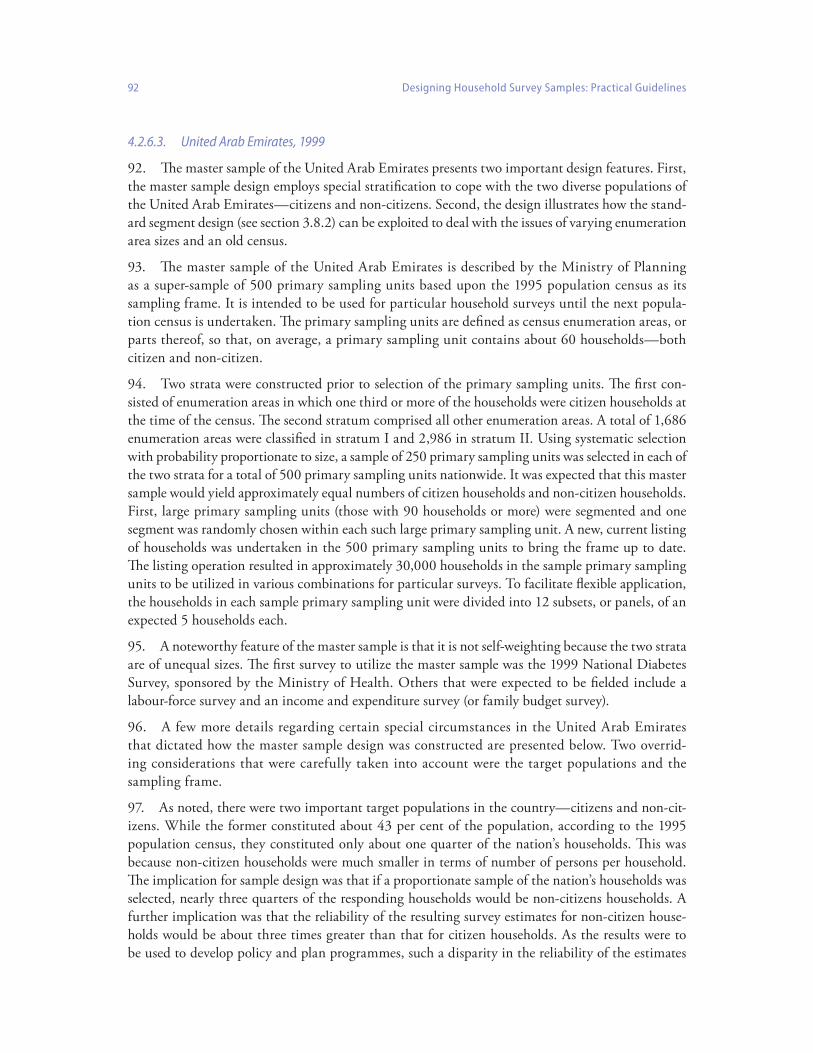
92 Designing Household Survey Samples: Practical Guidelines
United Arab Emirates, 19994.2.6.3.
The master sample of the United Arab Emirates presents two important design features. First, 92. the master sample design employs special stratification to cope with the two diverse populations of the United Arab Emirates—citizens and non‑citizens. Second, the design illustrates how the stand‑ard segment design (see section 3.8.2) can be exploited to deal with the issues of varying enumeration area sizes and an old census.
The master sample of the United Arab Emirates is described by the Ministry of Planning 93. as a super‑sample of 500 primary sampling units based upon the 1995 population census as its sampling frame. It is intended to be used for particular household surveys until the next popula‑tion census is undertaken. The primary sampling units are defined as census enumeration areas, or parts thereof, so that, on average, a primary sampling unit contains about 60 households—both citizen and non‑citizen.
Two strata were constructed prior to selection of the primary sampling units. The first con‑94. sisted of enumeration areas in which one third or more of the households were citizen households at the time of the census. The second stratum comprised all other enumeration areas. A total of 1,686 enumeration areas were classified in stratum I and 2,986 in stratum II. Using systematic selection with probability proportionate to size, a sample of 250 primary sampling units was selected in each of the two strata for a total of 500 primary sampling units nationwide. It was expected that this master sample would yield approximately equal numbers of citizen households and non‑citizen households. First, large primary sampling units (those with 90 households or more) were segmented and one segment was randomly chosen within each such large primary sampling unit. A new, current listing of households was undertaken in the 500 primary sampling units to bring the frame up to date. The listing operation resulted in approximately 30,000 households in the sample primary sampling units to be utilized in various combinations for particular surveys. To facilitate flexible application, the households in each sample primary sampling unit were divided into 12 subsets, or panels, of an expected 5 households each.
A noteworthy feature of the master sample is that it is not self‑weighting because the two strata 95. are of unequal sizes. The first survey to utilize the master sample was the 1999 National Diabetes Survey, sponsored by the Ministry of Health. Others that were expected to be fielded include a labour‑force survey and an income and expenditure survey (or family budget survey).
A few more details regarding certain special circumstances in the United Arab Emirates 96. that dictated how the master sample design was constructed are presented below. Two overrid‑ing considerations that were carefully taken into account were the target populations and the sampling frame.
As noted, there were two important target populations in the country—citizens and non‑cit‑97. izens. While the former constituted about 43 per cent of the population, according to the 1995 population census, they constituted only about one quarter of the nation’s households. This was because non‑citizen households were much smaller in terms of number of persons per household. The implication for sample design was that if a proportionate sample of the nation’s households was selected, nearly three quarters of the responding households would be non‑citizens households. A further implication was that the reliability of the resulting survey estimates for non‑citizen house‑holds would be about three times greater than that for citizen households. As the results were to be used to develop policy and plan programmes, such a disparity in the reliability of the estimates

Sampling frames and master samples 93
was not thought to be desirable or useful. The solution, in terms of sample design, was to treat the two disparate and unequal target populations as separate entities through the application of proper stratification as described above.
Another level of stratification was used as well, namely, geographical stratification, to ensure 98. appropriate distribution of the sample by emirate and by urban and rural. The file of enumeration areas was sorted in the following sequence prior to sample selection: first, the citizen stratum by urban, and within urban, by emirate, and within emirate by enumeration area codes arranged in ascending order by percentage citizen, followed by rural, emirate and enumeration area code; then, the non‑citizen stratum in the same sequence.
It was recognized that a key feature of the master sample frame must be a clear set of maps that 99. delineated the area units to be designated as the sample areas, that is to say, the primary sampling units. The area units had to be small enough to be conveniently listed but at the same time large enough so that they could be clearly defined with respect to natural boundaries (for ease of loca‑tion). Census enumeration areas were thought to be the only feasible area units that met these dual criteria. Unfortunately, maps were not used in the population census; and hence, the existing enu‑meration areas were not clearly defined in terms of known boundaries. As a result, it was necessary to ensure that good boundary information was developed for the master‑sample primary sampling units (enumeration areas).
Preparations for the master sample of primary sampling units made use of the “standard seg‑100. ment design”, described in chapter 3. It is a methodology that has been used successfully in many countries through both the Demographic and Health Surveys programme and the Pan Arab Survey of Maternal and Child Health (PAPCHILD).
It was decided to use the standard segment design because census enumeration areas in the 101. United Arab Emirates are quite variable in size. Standard segments of approximately 60 households were created. The number of standard segments was calculated in each sample primary sampling unit as the total number of households (that is, to say citizen plus non‑citizen) divided by 60 and rounded to the nearest integer.
For cases where the number of segments—that is, to say the measure of size—was two or 102. more, the Primary Sampling Unit was divided into area segments. This required a field procedure entailing a visit to the enumeration area (primary sampling unit) and the preparation of a sketch map using quick‑counting and map‑spotting of the dwellings (not the households). After segmentation, one segment was chosen from each primary sampling unit at random. That segment became the actual geographical area for sampling in the master sample. Another visit to the field was conducted to obtain a current list of the households in each sample segment. The latter procedure, necessary to bring the three‑year old master sample frame up to date, was consequently considered thought to be a vital component of the sampling operation.
The final operation for the master sample consisted of subdividing the newly listed households 103. in each sample segment into 12 systematic subsets or panels. One or more of the panels was to be used for particular surveys. Since the average size of the segment was about 60 households, each panel contained 5 households on average.
The main reason for having 12 panels was the flexibility provided by this number in forming 104. combinations for use in surveys. The actual choice for a given survey depended on various factors including the objectives of the survey, the desired cluster size and the overall sample size required for the

94 Designing Household Survey Samples: Practical Guidelines
survey. For example, two fifths of the primary sampling units were to be used in the National Diabetes Survey. Hence, 4 of the 12 panels of households within those primary sampling units were included. This combination yielded an overall sample plan of 200 primary sampling units with clusters of size 20 (that is, to say 4 times 5 households) and a total sample size of approximately 4,000 households.
Viet Nam, 20014.2.6.4.
The master sample of Viet Nam has two distinguishing features. It demonstrates the use of 105. two stages in selecting the master sample and of a third stage when applied to particular surveys. Second, it demonstrates how a master sample can be allocated to geographical domains.
The master sample, which is based on the 1999 census as the sampling frame encompasses 106. a two‑stage design. Primary sampling units were defined as communes in rural areas and wards in urban areas. They were defined in this way because it was decided that a minimum of 300 house‑holds would be necessary in each primary sampling unit to serve the master sample. Alternatively, enumeration areas were considered primary sampling units but they were too small and would have had to be combined with adjacent enumeration areas in order to qualify satisfactorily as primary sampling units. The latter task was thought to be much too tedious and time‑consuming. On the other hand, the number of communes/wards, that had to be combined because of their small size was only 529 out of the more than 10,000.
A total of 3,000 primary sampling units were selected by probability proportionate to size 107. for the master sample. Each sample primary sampling unit contained, on average, 25 enumeration areas in urban areas and 14 in rural areas. For the second stage of selection, three enumeration areas were selected in each sample primary sampling unit, using probability proportionate to size. The second‑stage units, enumeration areas, contained an average of approximately 100 households according to the 1999 census: 105 in urban areas and 99 in rural areas.
An objective of the master sample was to be able to provide fairly reliable data for each of Viet 108. Nam’s eight geographical regions. Sample selection was undertaken independently within each prov‑ince. Thus, provinces served as strata for the master sample. It was desired to over select the sample in certain small provinces that contained very small populations. Accordingly, the allocation of the sample among provinces was made by the method of probability proportionate to the square root of the size of the province. Proportional allocation between urban and rural areas was used.
In addition to the provincial‑level stratification mentioned above, implicit geographical strati‑109. fication within provinces was used. In applying the master sample to specific surveys, subsets of the enumeration areas were to be used—for example, one third of them for the Multi‑purpose House‑hold Survey. For survey applications, a third stage of selection is administered in which a fixed number of households is selected from each sample enumeration area. That number may vary by survey and by urban and rural. For example, 20 households per enumeration area might be chosen for rural enumeration areas and 10 per enumeration area for urban enumeration areas.
Mozambique, 1998‑19994.2.6.5.
The master sample of Mozambique illustrates a case in which a single‑stage selection of pri‑110. mary sampling units was to be used for all of the Government‑sponsored national surveys in the nation’s intercensal household survey programme. It also illustrates how a flexible master sample can be adapted to meet the measurement objectives of a particular survey.

Sampling frames and master samples 95
Master‑sample primary sampling units in Mozambique were defined and sampled in a 111. straightforward way, as described in various parts of this handbook. The primary sampling units were constructed from the 1997 Population Census as the sample frame. They consisted of geographical groupings of, generally, from three to seven census enumeration areas, which contained about 100 households on average. The master‑sample primary sampling units were selected using probability proportionate to size.
A total of 1,511 primary sampling units were selected to provide the framework for sampling 112. to be applied for Mozambique’s integrated system of household surveys. The master‑sample primary sampling units were divided into panels, each constituting a systematic subset and therefore a prob‑ability sample in its own right. There are 10 such panels of about 151 primary sampling units each. In the five‑year (2000‑2004) Plan, the Core Welfare Indicators Questionnaire conceived by the World Bank was the first survey to make use of the master sample.
The sample plan for the Core Welfare Indicators Questionnaire was designed with two meas‑113. urement objectives in mind. The first was to obtain the relevant indicators necessary to profile the well‑being of persons and households in Mozambique. The second was to provide reliable estimates of these indicators at the national level, for urban and rural areas separately and for each of the 11 prov‑inces in the country. The sampling methodology for the Core Welfare Indicators Questionnaire utilized the Mozambique master sample to choose about 14,500 households in a stratified, clustered design. Accordingly, the first stage of selection was, of course, the master‑sample primary sampling units.
The second stage of selection for the Core Welfare Indicators Questionnaire was a subsample 114. of the master sample primary sampling units. A total of 675 primary sampling units were subsampled from the 1,511 in the master sample. They were selected systematically with equal probability and, in addition, equally allocated among the 11 provinces of Mozambique. At the third stage a sample of one enumeration area was selected in each of the primary sampling units for the Core Welfare Indicators Questionnaire. Thus, there were 675 clusters in the Questionnaire sample—475 rural and 200 urban. The enumeration areas were selected with equal probability because their sizes were roughly the same—as mentioned above, about 100 households on average, although there was vari‑ability. The final stage of selection occurred following fieldwork in which the Instituto Nacional de Estatistica (INE) visited the clusters to compile a fresh list of households in order to bring the 1997 sample frame up to date. From the lists so compiled, a systematic sample of 20 households in rural areas and 25 in urban was selected for the Questionnaire survey interviews. Sample selection for the Questionnaire was thus a four‑stage selection process, although the master sample upon which it was based was single‑stage.
Two design features for the Core Welfare Indicators Questionnaire, illustrate the flexibility with 115. which the master sample can be adapted to fit the particular requirements for a survey application.
First, in utilizing the master sample for the Core Welfare Indicators Questionnaire, there had 116. been interest on the part of the Instituto Nacional de Estatistica in using the panels that had already been designated, as mentioned above. Given the desire to have about 600 primary sampling units for the Questionnaire, it was hoped that four of the panels could be used. The idea was discarded, however, when it was realized that the number of panels that would be necessary for the Question‑naire would be different for each province, because the measurement objective required more or less the same sample size by province. Instead, the 675 primary sampling units necessary for the Ques‑tionnaire were selected systematically from the entire master‑sample file without regard to panels. This departure from the original intent of the master sample which was, to provide a proportionate

96 Designing Household Survey Samples: Practical Guidelines
sample by province occurred because equal reliability was desired at the provincial level for the Questionnaire, in contrast to the original design of the master sample. In the master‑sample plan, as originally conceived, national‑level estimates had been expected to take precedence.
A second important issue regarding the Questionnaire sample design was the cluster size. It 117. was agreed that cluster sizes should be different for urban and rural households on the grounds that the sample design effect, or deff, was higher in rural areas where most of the economic livelihood was derived from subsistence farming. In other words, households in a rural area were likely to have very similar characteristics. The master sample afforded the possibility of selecting a different fixed number of households (25 and 20, respectively, in urban and rural areas) in the final stage.
Summary guidelines4.3. The present section summarizes the main guidelines to be extracted from this chapter. Pre‑118.
sented in checklist format and, as in chapter 3, more as rules of thumb than as fixed recommenda‑tions, they suggest:
Using sample frames that are as complete, accurate and current as possible.•
Ensuring that the sample frame covers the intended target population.•
Using the most recent census as frame for household surveys if possible.•
Defining primary sampling units in the frame in terms of area units such as census • enu‑meration areas with mapped, well‑delineated boundaries and for which population figures are available.
Using the census list of households as the frame at the last stage only if it is very recent—•usually no more than one year old.
Using dual or multiple frames with caution by ensuring that procedures are in place for •dealing with duplications.
Updating the census frame if more than two years old—nationwide or in specifically •targeted areas known to have high growth, to encompass:
Using quick‑count canvassing to update the old frame.•
In sample clusters, updating by making a fresh list of households.•
Updating only in sample clusters if census frame is no more than two years old, to •encompass:
Updating by making a fresh list of households.•
Using the master sample or master‑sample frame only when a large‑scale continuing survey •programme is planned or under way.
Defining master‑sample primary sampling units that are large enough or numerous enough •to sustain many surveys, or repeat survey rounds, during the intercensal period.
Updating master‑sample frames using the same guidelines as suggested above for sin‑•gle‑survey frames.
Employing system of sample rotation—either of households or • primary sampling units—in repeat surveys that use master samples.

Sampling frames and master samples 97
References and further reading
Cochran, W. G. (1977), Sampling Techniques, 3rd ed., New York: Wiley.
Hansen, M. H., W. N. Hurwitz, and W. G. Madow (1953). Sample Survey Methods and Theory, New York: Wiley.
International Statistical Institute (1975). Manual on Sample Design. World Fertility Survey Basic Documentation, Voorburg, Netherlands.
Kalton, G. (1983). Introduction to Survey Sampling, Beverly Hills, California: Sage. Publications Kish, L. (1965), Survey Sampling. New York: Wiley.
League of Arab States (1990). Sampling Manual, Arab Maternal and Child Health Survey, Basic Documentation 5. Cairo: Pan Arab Project for Child Development (PAPCHILD).
Macro International, Inc. (1996). Sampling Manual. DHS‑III Basic Documentation, No. 6. Calverton, Maryland.
Pettersson, Hans. (2001), Mission report: recommendations regarding design of master sample for household surveys of Viet Nam. Unpublished. General Statistical Office, Hanoi. 25 November
________ (2005). Design of master sampling frames and master samples for household surveys in developing countries. In Household Sample Surveys in Developing and Transition Countries. Studies in Methods, No. 96 Sales No. E.05.XVII.6.
Turner, A. (1998), Mission report to the Kingdom of Cambodia, National Institute of Statistics, 11‑24 November. National Institute of Statistics, Phnom Penh: Unpublished.
________ (1999), Mission report to United Arab Emirates, Ministry of Health and Central Department of Statistics 23 January–3 February. Abu Dhabi: Unpublished. Central Department of Statistics.
________ (2000). Mission report to Mozambique, Instituto Nacional de Estatistica, 13‑26 August. Instituto Nacional de Estatistica, Maputo: Unpublished.
United Nations Statistics Division (1984). Handbook of Household Surveys (Revised Edition). Studies in Methods, No. 31. Sales No. E.83.XVII.13.
________ (1986), National household Survey Capability Programme: Sampling frames and sample designs for integrated household survey programmes. Preliminary Version. DP/UN/INT‑84‑014/5E. New York: United Nations Department of Technical Co‑operation for Development and Statistical Office.
United Nations Children’s Fund (2000). End‑Decade Multiple Indicator Survey Manual. New York: UNICEF chapter 4.
United States Bureau of the Census (1978). Current Population Survey Design and Methodology. Technical Paper 40. Washington, D.C.: Bureau of the Census.
Verma, Vijay (1991). Sampling Methods. Training Handbook. Tokyo: Statistical Institute for Asia and the Pacific.
World Bank (1999). Core Welfare Indicators Questionnaire (CWIQ) Handbook. Washington D.C.: World Bank., chapter 4.


99
Chapter 5
Documentation and evaluation of sample designs
Introduction5.1.
The present chapter, though comparatively short, nevertheless has a central role in the hand‑1. book. Documentation and evaluation of sample designs in particular and survey methodology in general are too often neglected in the rush to release survey findings. This is especially true in countries with little prior experience in conducting household surveys, where metadata are often poorly documented in survey worksheets and reports. In some countries, documentation of survey procedures including sample implementation is little valued. Thus, there is no tradition in place of requiring it. While researchers undertake to analyse data generated in surveys, they should also be interested in knowing the methodologies related to sample design. A number of documents should, therefore, be prepared detailing the procedures employed in the survey.
Evaluation of the survey results is often completely ignored. In consequence, errors creep into 2. survey analysis. This is generally due to the fact that budgetary restrictions often preclude the devel‑opment of any formal studies or methods to assess the abundance of non‑sampling errors that may crop up in household surveys. Yet, there are other barometers of data quality that should be readily available (such as rate of non‑response) and these, too, are often not mentioned in survey reports.
This chapter also emphasizes the importance of presenting relevant information to users on 3. known limitations of the data, even when formal evaluation studies have not been conducted; but it is important, in this regard, to note that the discussion of techniques for conducting formal evalu‑ations of survey methodology, of which there are many, is beyond its scope.1 Instead, the chapter focuses on what information should be given to users to help them in evaluating the quality of the survey, concentrating on sampling aspects.
Need for, and types of, sample documentation and evaluation5.2. There are two types of documentation needed in household surveys. The first type comprises 4.
careful records of the survey and sampling procedures as they are being carried out operationally in
1 Special studies that are designed to evaluate specific types of non‑sampling error in surveys include re‑interview surveys (for evaluating response variability), post‑enumeration surveys (for coverage and content evaluation), interpenetrating samples (for evaluating interviewer variability), reverse record checks (for evaluating respondent recall errors) and so forth.

100 Designing Household Survey Samples: Practical Guidelines
the survey process. Without such documentation, errors creep into survey analysis. For example, prob‑abilities of selection may not be fully known at the time of analysis without careful record‑keeping.
The sampling technician should therefore take necessary steps to carefully document not only 5. the sample plan for the particular survey undertaken but also its implementation. Sample designs often require adaptations at various stages of the fieldwork because of unforeseen situations that arise in the conduct of the survey. It is important to record—step by step—all the procedures used in car‑rying out the sample plan to make sure that the implementation is faithful to the design. When this is not the case, it is even more important to document all the departures from the design, even minor ones. This information will be necessary later, at the analysis stage, should any adjustments need to be made. Moreover, documentation of this type is indispensable for planning future surveys.
The second type of documentation comprises reports. There ought to be two kinds of technical 6. reports prepared for every household survey: a fairly brief, user‑friendly description of the survey methodology including the sample plan and its implementation; and a more detailed description of the survey methodology. The former would typically cover the “technical” sections (or appendices) of the various substantive reports released to discuss and interpret the substantive findings of the survey,2 including a subsection on what is known about the limitations of the data (see below).
The second kind of technical report is intended more for professional researchers, social scien‑7. tists and statisticians than for policymakers or the general public, should contain a more detailed description of the survey methodology and should stand on its own rather than be part of a series of substantive reports. The United States Bureau of the Census (1978) has produced an excellent ver‑sion of such a report. Of course, it is preferable to have the detailed technical report and the regular survey reports produced concurrently, although the former is typically prepared, much later, if at all. It is also useful, to have the technical report, or an abridged version, published in a statistical journal so as to ensure its longevity.
Reports of both types are so important that it is recommended that national statistical Offices 8. assign a special office or officer to prepare them routinely for household surveys.
Labels for design variables5.3. The present section and sections 5.2‑5.7, discuss documentation of the first type, which involves 9.
record‑keeping of survey processes related to sampling.
The units of selection identified at each stage must be clearly and uniquely labelled. In a multi‑10. stage design, this will mean establishing codes for the primary, secondary, tertiary and ultimate sampling units (depending upon how many stages there are in the design). Normally a four‑digit code will suffice for the first stage of selection and a three‑digit code for the remaining stages. Geo‑graphical domains must also be properly labelled. In addition, the administrative codes identifying the geographical, administrative structure of the areas to which the sampling units belong should be part of the labelling process. The analysis units should also be explicitly identified.
Example
Suppose that a sample of 1,200 primary sampling units, defined as census enumeration areas, is selected for a two‑stage design, with 600 in each of two domains defined as urban and rural. A
2 Guidelines on what to include in the report on findings from a sample survey can be found in a report of the United Nations Subcommission on Statistical Sampling, (United Nations, 1964).
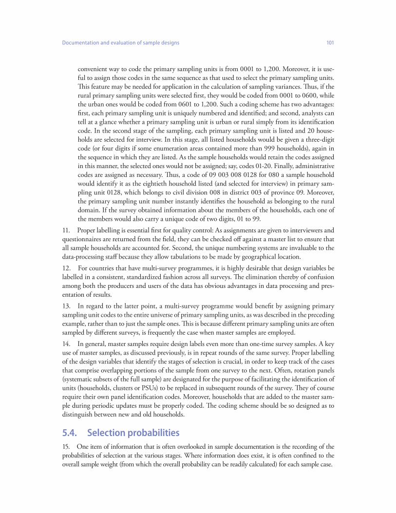
Documentation and evaluation of sample designs 101
convenient way to code the primary sampling units is from 0001 to 1,200. Moreover, it is use‑ful to assign those codes in the same sequence as that used to select the primary sampling units. This feature may be needed for application in the calculation of sampling variances. Thus, if the rural primary sampling units were selected first, they would be coded from 0001 to 0600, while the urban ones would be coded from 0601 to 1,200. Such a coding scheme has two advantages: first, each primary sampling unit is uniquely numbered and identified; and second, analysts can tell at a glance whether a primary sampling unit is urban or rural simply from its identification code. In the second stage of the sampling, each primary sampling unit is listed and 20 house‑holds are selected for interview. In this stage, all listed households would be given a three‑digit code (or four digits if some enumeration areas contained more than 999 households), again in the sequence in which they are listed. As the sample households would retain the codes assigned in this manner, the selected ones would not be assigned; say, codes 01‑20. Finally, administrative codes are assigned as necessary. Thus, a code of 09 003 008 0128 for 080 a sample household would identify it as the eightieth household listed (and selected for interview) in primary sam‑pling unit 0128, which belongs to civil division 008 in district 003 of province 09. Moreover, the primary sampling unit number instantly identifies the household as belonging to the rural domain. If the survey obtained information about the members of the households, each one of the members would also carry a unique code of two digits, 01 to 99.
Proper labelling is essential first for quality control: As assignments are given to interviewers and 11. questionnaires are returned from the field, they can be checked off against a master list to ensure that all sample households are accounted for. Second, the unique numbering systems are invaluable to the data‑processing staff because they allow tabulations to be made by geographical location.
For countries that have multi‑survey programmes, it is highly desirable that design variables be 12. labelled in a consistent, standardized fashion across all surveys. The elimination thereby of confusion among both the producers and users of the data has obvious advantages in data processing and pres‑entation of results.
In regard to the latter point, a multi‑survey programme would benefit by assigning primary 13. sampling unit codes to the entire universe of primary sampling units, as was described in the preceding example, rather than to just the sample ones. This is because different primary sampling units are often sampled by different surveys, is frequently the case when master samples are employed.
In general, master samples require design labels even more than one‑time survey samples. A key 14. use of master samples, as discussed previously, is in repeat rounds of the same survey. Proper labelling of the design variables that identify the stages of selection is crucial, in order to keep track of the cases that comprise overlapping portions of the sample from one survey to the next. Often, rotation panels (systematic subsets of the full sample) are designated for the purpose of facilitating the identification of units (households, clusters or PSUs) to be replaced in subsequent rounds of the survey. They of course require their own panel identification codes. Moreover, households that are added to the master sam‑ple during periodic updates must be properly coded. The coding scheme should be so designed as to distinguish between new and old households.
Selection probabilities5.4. One item of information that is often overlooked in sample documentation is the recording of the 15.
probabilities of selection at the various stages. Where information does exist, it is often confined to the overall sample weight (from which the overall probability can be readily calculated) for each sample case.

102 Designing Household Survey Samples: Practical Guidelines
A particularly important detail for proper documentation must be considered when subsam‑16. pling is conducted in the field during data collection, as may happen when a sample segment/cluster is too large. For example, as discussed earlier, an unexpectedly large cluster may have to be segmented into, say, four parts of roughly equal size. One part is then selected at random for listing and interviewing. In that case, the overall probability of the sampled segment (and the households/persons selected therein) is one fourth that of the original cluster; and its weight is thus the inverse of one fourth, or four. That weighting factor has to be reflected in the calculations when the data are analysed.
Subsampling may also occur when there is more than one household in a dwelling (when the 17. dwelling is the listing unit). One option, which is unbiased, is for the survey manager to interview all the households found: this is often the approach if there are only two. However, there are, say, five when one was expected, cost considerations may dictate that only one of them—randomly picked, of course—is to be interviewed. Again, careful recording of the subsample rate (1/5 in this example) is essential so that the probability of selection for the affected household can be accurately calculated by the sampling staff and the weight thus properly adjusted (by a factor of 5).
It is also useful to record the probabilities of selection at each stage of selection as mentioned in 18. the opening paragraph of the present section. For example, the probability of selecting each primary sampling unit is different whenever probability proportionate sample sampling is used. This is true even if the overall sample design is self‑weighting. If the probabilities of selection of primary sam‑pling units are ignored or are erroneously recorded, it may not be possible to determine the overall sampling weights. For example, it is useful to know what the original probabilities of selection are in order to accurately determine the subsampling procedures.
Response rates and coverage rates 5.5. at various stages of sample selection
As part of the process of evaluating the implementation of the sample survey, it is essential to 19. provide information to users on response rates and coverage rates. It is useful to make available as much detail as possible. Thus, it is important to provide not only the rate of response (or its comple‑ment, the rate of non‑response) but also a tabulation of the reasons for non‑response. Categories of non‑response would likely include the following:
No one at home•
Vacant dwelling unit•
Demolished or uninhabitable dwelling unit•
Refusal•
Away temporarily (holiday, etc.)•
The definition of response rate, in terms of which categories are included, may vary from 20. country to country. Typically, however, completed response includes the first, fourth and fifth of the above categories. Those categories comprise cases in which a response should be obtained if at all possible. Vacant and demolished units are usually ignored (in calculating the response rate) on the grounds that by definition, it is not possible, to obtain a response in such units. Thus, for example, a country may select 5,000 households with the following results: 4,772 completed interviews, 75

Documentation and evaluation of sample designs 103
cases of “no one at home”, 31 vacant dwellings, 17 demolished units, 12 refusals and 93 cases of “away temporarily”. The response rate would be calculated, ordinarily excluding the vacant and demolished units, as 4,772/(5,000–31–17) or 96.4 per cent.
When the survey target populations include both households—for variables such as household 21. income or access to services—and individuals (for, say, health status of adult women), it is customary to calculate response rates at both the household and the individual level. For example, 98 per cent of the households may respond; but within the responding households, a small proportion of the individuals may be non‑respondents.
Often, whole clusters are not interviewed for various reasons including issues of security such 22. as civil strife or disorder and lack of accessibility due to the terrain or the weather. Frequently when such problems arise, substitute clusters are selected, a procedure that is seriously biased because the inhabitants of the substitute clusters are almost always likely to differ in very significant ways from those in the replaced clusters. Nevertheless, when such substitutions are made, it is incumbent upon the survey team to record the number and location of such clusters. Moreover, it is also important to provide some information on under‑coverage in such cases. This might be done by estimating, to the extent possible, the number of persons in the target population(s) thought to reside in the areas by the represented replaced clusters.
It is useful to note that problems of the type mentioned directly above can be reduced somewhat 23. by identifying in advance of sample selection the areas of the country that are “out of scope” for survey interviewing owing to security or accessibility concerns. Those identified should be documented and excluded from the survey universe before sample selection. The excluded areas should be documented in the report and a statement included that the results of the survey do not apply to the excluded area.
Weighting: base weights, non‑response and other 5.6. adjustments
Calculation of survey weights is presented in chapter 6. The present chapter emphasizes the 24. importance of documenting those calculations.
Weighting for household surveys generally involves up to three operations—calculation of the 25. base or design weights, adjustments for non‑response, and adjustments for post‑stratification. In many applications, only the design weights are used, while in others, the design weights may be adjusted by an additional factor to reflect non‑response. In comparatively few applications, the weighting may reflect another factor, either with or without non‑response adjustments, intended to adjust the population distribution obtained from the sample so as to make it agree with the distribution from an independent source of data such as a recent census. This is often referred to as post‑stratified weighting. In some applications no weighting is done at all; this would occur only when two conditions are met: that the sample be completely self‑weighting and that the data generated be restricted to percentage distributions, proportions and ratios, as opposed to estimated totals or absolutes.
When weighting is used, it is necessary of course to carefully record the calculations. As men‑26. tioned previously, the weights (or probabilities) at each stage of selection should be calculated and recorded. Also, separate weights in each phase of data operations should be recorded, that is to say, (a) design weights, (b) design weights after multiplication by the non‑response adjustment factor(s) and (c) the design weights in (b) after adjustment factors for post‑stratification have been applied.

104 Designing Household Survey Samples: Practical Guidelines
It is important to note that design weights will differ for each domain whenever the sample 27. design includes domain estimation. In other words, even when the sample is self‑weighting within domains, each domain will have its own distinct weight. Furthermore, each domain will have a dif‑ferent set of weights if the design is not self‑weighting within domains. In addition, it should be noted that non‑response adjustments are often applied separately by important geographical sub‑areas such as major regions, irrespective of whether domain estimation is present in the design. Finally, the design weight itself may be multiplied by an additional factor for particular clusters or households. This would be done whenever subsampling (see section 5.3) is used.
Information on sampling and survey implementation costs5.7. While household surveys are usually budgeted for very carefully, it is equally important to keep 28.
records of actual expenditures of their various operations. Recording of survey costs is useful, for example, for planning master samples and record‑keeping, of various survey activities, is important for planning for future surveys.
When master samples are utilized, there is an initial large start‑up cost to effectuate its devel‑29. opment. It generally includes aspects of (a) computer manipulation of census files to establish the sample frame, (b) mapping or cartographic work to create primary sampling units and (c) compu‑ter‑selection of sample primary sampling units. As mentioned in the preceding chapter, the cost of the start‑up operations is often shared by the ministries that will make use of the master sample during its life cycle. Those costs should also be distributed over all the surveys for which the master sample is intended, to the extent that they are all known about in advance. It is therefore essential that very careful record‑keeping in respect of developing the master sample as well as planning the sampling aspects of future surveys, be maintained.
Once the master sample is in place, records on the cost with respect to maintaining it need to 30. be compiled. As noted previously, updating of master samples takes place periodically and, its cost, of course, needs to be carefully monitored.
Sampling operations for which cost figures ought to be regularly obtained include those in the 31. following list which applies to both one‑time sample surveys and master samples:
(a) Salaries for sample design including fees for any outside consultant;(b) Field costs for updating the sample frame, including personnel and preparation of auxiliary
materials such as maps;(c) Computer costs for preparing the sample frame for selecting the sample of primary sampling
units;(d) Personnel costs for selecting the sample of primary sampling units (if not carried out by
computer);(e) Field costs for conducting the listing operation in the penultimate‑stage sampling units
including personnel and the preparation of materials such as cluster folders;( f ) Personnel costs for collecting data from sample of households within the sample clusters.
In addition to the sampling costs of the survey, records should be kept relating to implementa‑32. tion costs. Such costs may include: enumerators’ and supervisors’ wages; daily subsistence allowance and field expenses of regular staff members of the survey organisation; travel expenses; office supplies; training expenses; fuel costs; communication services and data processing.

Documentation and evaluation of sample designs 105
Evaluation: limitations of survey data5.8. Much of the documentation on proper record‑keeping discussed above, in addition to being 33.
important in processing the survey results is useful for evaluating aspects of the sample design and survey implementation. Information on response rates, for example, helps to assess whether bias from non‑response is serious or not. Sampling cost information may be used to evaluate the “economic” effectiveness of the sample design and its utility for future surveys.
As stated previously, formal evaluation of sample surveys covers multiple facets of non‑sam‑34. pling error that are much beyond the scope of this Handbook (see United Nations (1984)—for a comprehensive treatment of the subject). It should, however, be mentioned that the evaluation of nonsampling error should, for example, include activities in the operational and processing areas. On the other hand, sampling error can be estimated and is discussed further below.
Despite the fact that formal evaluation studies are not often conducted for household surveys, 35. it is nevertheless crucial that the survey documentation include information on the limitations of the data. A brief section of the substantive reports on findings, often entitled simply, “Limitations of the survey data” should be devoted to this subject. In that section, the reader must be informed of both sampling and non‑sampling aspects of survey error.
A valuable publication of the United States Bureau of the Census (1974) describes how to 36. present information on survey errors. The following specimen paragraphs from that publication (appendix I, p. I‑1) suggest the kind of information that should be presented to users when survey findings are released:
The statistics in this report are estimates derived from a sample survey. There are two types of errors possible in an estimate based on a sample survey—sampling and nonsampling. Sampling errors occur because observations are made only on a sample, not on the entire population. Nonsampling errors (discussed in chapter 8) can be attributed to many sources: inability to obtain information about all cases in the sample, definitional difficulties, differences in the interpretation of questions, inability or unwillingness to provide correct information on the part of respondents, mistakes in recording or coding the data obtained, and other errors of collection, response, processing, coverage, and estimation for missing data. Nonsampling errors also occur in complete censuses. The accuracy of a survey result is determined by the joint effects of sampling and nonsampling errors.
The particular sample used in this survey is one of a large number of all possible samples of the same size that could have been selected using the same sample design. Estimates derived from the different samples would differ from each other. The deviation of a sample estimate from the average of all possible samples is called the sampling error. The standard error of a survey estimate is a measure of the variation among the estimates from the possible samples and thus is a measure of the precision with which an estimate from a particular sample approximates the average result of all possible samples. The relative standard error is defined as the standard error divided by the value being estimated.
As calculated for this report, the standard error also partially measures the effect of nonsampling errors but does not measure any systematic biases in the data. Bias is the difference, averaged over all possible samples, between the estimate and the desired value. Obviously, the accuracy of a survey result depends upon both the sampling and nonsampling errors, measured by the standard error, and the bias and other types of nonsampling error, not measured by the standard error.

106 Designing Household Survey Samples: Practical Guidelines
As implied above, an important component of sample evaluation is estimation of sampling 37. errors, which should be undertaken for the key survey estimates. As discussed previously, one of the distinguishing characteristics of a probability sample is that the sample itself can be used to estimate standard errors. Methods of variance and standard error estimation are discussed in detail in chap 6. In addition, there are efficient and reliable software packages available to estimate standard errors that should be taken advantage of whenever possible.
Generally, estimates of standard errors are prepared for the key characteristics of interest in 38. the survey, since it is neither practical nor necessary to calculate them for all the items. The standard errors of course provide the means for users to evaluate the reliability of the survey estimates and to construct confidence intervals around the point estimates.
The standard errors may also be used to evaluate the sample design itself. A particularly useful 39. statistic for doing this is the sample design effect, deff, or, more precisely, deft, the square root of deff. It is a fairly straightforward to calculate deft for every data item for which the standard error is estimated. It entails only dividing the estimated standard error, for a given item, by the standard error from a simple random sample of the same sample size, namely, pq/n, where p is the estimated proportion; q is 1–p and n is the sample size. The exercise serves to confirm or refute the design effects that were assumed when the sample was being designed, since the actual deffs or defts cannot be known until after the survey has been conducted, the data have been processed and the standard errors have been estimated.
The sampling statistician can use the calculated design effects to determine whether the cluster 40. sizes are of reasonable size for key data items and may take corrective action if necessary. For example, if deft is much larger than anticipated for certain key items, the sample for a future survey may be so designed as to use smaller cluster sizes.
Summary guidelines5.9. The present section summarizes in checklist format the main guidelines contained in this 41.
chapter, which, as in preceding chapters, are presented more as rules of thumb than as fixed recom‑mendations and:
Documenting sampling aspects of surveys in two ways: proper record‑keeping and provi‑•sion of technical information to users.
Keeping detailed records of sampling processes including costs.•
Developing codes for sample design variables: administrative areas, • primary sampling units, clusters, households, persons, etc.
Striving for standardized coding of design variables that are consistent over all surveys.•
Recording all deviations or departures from other original sample plan that occur in the •implementation of survey.
Calculating and recording probabilities of selection at each stage of sampling.•
Recording, especially, information on subsampling that occurs in fieldwork.•
Recording information on the number and types of non‑response.•
Recording design weights, adjustments for non‑response and post‑stratified adjustments.•

Documentation and evaluation of sample designs 107
Keeping detailed cost records of each operation in sample design and implementation.•
In master sampling, keeping cost records of both its development (start‑up) and its main‑•tenance.
Preparing technical reports, for users, on sampling and survey methodology.•
Preparing brief report on limitations of data for all substantive publications that report •on survey results.
Preparing a more intensive technical report on all aspects of sampling methodology.•
Calculating sampling errors for key variables and presenting these in technical reports.•
Calculating design effects (• deff or deft) for key variables.
Assigning an officer to be in charge of documentation.•
References and further reading
Casley, D. J., and D. A. Lury, (1981). Data Collection in Developing Countries. Oxford, United Kingdom: Clarendon Press.
International Statistical Institute (1975). Manual on Sample Design. World Fertility Survey Basic Documentation, Voorburg, Netherlands.
League of Arab States (1990). Sampling Manual, Arab Maternal and Child Health Survey, Basic Documenta‑tion 5. Cairo: Pan Arab Project for Child Development (PAPCHILD.
Macro International, Inc. (1996), Sampling Manual. DHS‑III Basic Documentation No. 6. Calverton, Maryland.
United Nations (1964). Recommendations for the Preparation of Sample Survey Reports (Provisional Issue). Statistical Papers, Series C, No. 1, Rev.2.
________ (1984), Handbook of Household Surveys, (Revised Edition).Studies in Methods, No. 31. Sales No. E.83.XVII.13.
United States Bureau of the Census (1974). Standards for Discussion and Presentation of Errors in Data. Technical Paper 32. Washington, D.C.: United States Bureau of the Census.
________ (1978). Current Population Survey Design and Methodology. Technical Paper 40. Washington, D.C.: Bureau of the Census.
World Bank (1999). Core Welfare Indicators Questionnaire (CWIQ ) Handbook. Washington, D.C.: World Bank.


109
Chapter 6
Construction and use of sample weights
Introduction6.1.
The present chapter discusses the various stages in the development of sample weights and their 1. use in computing estimates of characteristics of interest from household survey data. In particular, the adjustment of sample weights to compensate for various imperfections in the selected sample is described. Attention is restricted to descriptive estimates that are widely produced in most survey reports. The important ideas presented are illustrated using real examples of current surveys con‑ducted in developing countries, or of ones that mimic real survey situations.
Need for sampling weights6.2. Household surveys are, in general, based on complex sample designs, primarily to control cost. 2.
The resulting samples are likely to have imperfections that might lead to bias and other discrepancies between the sample and the reference population. Such imperfections include the selection of units with unequal probabilities, non‑coverage of the population and non‑response. Sample weights are needed to correct these imperfections and thereby derive appropriate estimates of characteristics of interest. In summary, the purposes of weighting are to:
(a) Compensate for unequal probabilities of selection;(b) Compensate for (unit) non‑response;(c) Adjust the weighted sample distribution for key variables of interest (for example, age, race,
and sex) so as to have it conform to a known population distribution.
The procedures used for each of these scenarios are discussed in detail in the sections that follow. 3. Once the imperfections in the sample are compensated for, weights can be used in the estimation of population characteristics of interest and also in the estimation of sampling errors of the survey estimates generated.
When weights are not used to compensate for differential selection rates within strata (whenever 4. the sample is so designed) and for the sample imperfections mentioned above, the resulting estimates of population parameters will, in general, be biased. See sections 6.3, 6.4 and 6.5 for examples of the weighting procedures employed under each scenario, including a comparison of the weighted and unweighted estimates in each case.

110 Designing Household Survey Samples: Practical Guidelines
Overview6.2.1. Section 6.3 deals with the development of sampling weights in the context of a multistage 5.
sample design, including the adjustment of sample weights to account for duplicates in the sample and for units whose eligibility for the survey is not known at the time of sample selection. Section 6.4 discusses weighting for unequal probabilities of selection; provides several numerical examples, including a case study of weight development for a national household survey; and, in conclusion, discusses self‑weighting samples. The issues of non‑response and non‑coverage in household sur‑veys are addressed in sections 6.5 and 6.6, respectively. Sources and consequences of non‑response and non‑coverage are discussed. Methods for compensating for non‑response and non‑coverage are also presented, including numerical examples illustrating the adjustment of sample weights for non‑response and non‑coverage. Section 6.7 discusses the issue of inflation in the variance of survey estimates as a result of the use of sample weights in the analysis of household survey data. A numeri‑cal example is also provided to illustrate the calculation of the increase in variance due to weighting. Section 6.8 discusses the issue of weight trimming and presents an example of a trimming procedure by which the trimmed weights are rescaled in such a way as to make them add up to the sum of the original weights. Some concluding remarks are offered in section 6.9.
Development of sampling weights6.3. Once the probabilities of selection of sampled units have been determined, the construction of 6.
sampling weights can begin. The probability of selection of a sampled unit depends on the sample design used to select the unit. Chapter 3 provided detailed descriptions of the most commonly used sampling designs and the probabilities of selection corresponding to these designs. It is assumed throughout that the probabilities of selection have been determined.
The development of sampling weights is sometimes considered to be the first step in the analysis 7. of the survey data. It usually starts with the construction of the base or design weight for each sampled unit so as, to reflect their unequal probabilities of selection. The base weight of a sampled unit is the reciprocal of its probability of selection for inclusion in the sample. In mathematical notation, if a unit is included in the sample with probability pi, then its base weight, denoted by wi, is given by
For example, a sampled unit selected with probability 1/50 represents 50 units in the population 8. from which the sample was drawn. Thus, sample weights act as inflation factors designed to represent the number of units in the survey population that are represented by the sample unit to which the weight is assigned. The sum of the sample weights provides an unbiased estimate of the total number of units in the target population.
For multistage designs, the base weights must reflect the probabilities of selection at each 9. stage. For instance, in the case of a two‑stage design in which the ith PSU is selected with probabil‑ity pi at the first stage, and the jth household is selected within a sampled PSU with probability pj(i) at the second stage, then the overall probability of selection (pij) of each household in the sample is given by the product of these two probabilities, or
wi pi=1 (6.1)
pij = pi* pj(i), (6.2)

Construction and use of sample weights 111
and the overall base weight of the household is obtained as before, by taking the reciprocal of its overall probability of selection. Correspondingly, if the base weight for the jth household is wij,b, the weight attributable to compensation for non‑response is wij,nr, and the weight attributable to the compensation for non‑coverage is wij,nc, then the overall weight of the household is given by
Adjustments of sample weights for unknown eligibility6.3.1. During data collection in household surveys, there are sometimes instances when the eligibility 10.
of a household is in question. For example, the interviewer may not find anyone home at a sampled dwelling unit at the time of data collection or after repeated visits. In such a case, it is not known whether the dwelling unit is occupied or not. If it is actually occupied, then it should be classified as a non‑responding dwelling unit (under the category “not at home”). Otherwise, it is out of scope for the survey and therefore ineligible to be counted as a sample unit. Sometimes, interviewers assume that if no one is found in a dwelling unit during repeated visits, then that dwelling unit is unoc‑cupied and hence ineligible. This is, in general, an incorrect assumption, and one that often leads to erroneously inflated response rates.
When the eligibility of some sampled dwelling units is unknown, their weights must be adjust‑11. ed to account for this fact. The idea is to make some assumptions that would permit the estimation of the proportion of dwelling units with unknown eligibility that are actually eligible. The simplest approach is to take the proportion of sampled dwelling units known to be either eligible or ineligible, and apply that to those of unknown eligibility. For instance, suppose that a sample of 300 dwelling units have the response dispositions set out in table 6.1.
Note that the proportion of dwelling units of known eligibility that are actually eligible is 12. (215+25)/(215+25+10) = 0.96. We can therefore assume that the same proportion (0.96) of the dwelling units with unknown eligibility can be considered eligible. In other words, 96 per cent of the 50 dwelling units with unknown eligibility (or 48 dwelling units) are actually eligible. We then adjust the weights of the eligible dwelling units (completed interviews and eligible non‑respondents) using an adjustment factor defined as follows:
wij = wij,b * wij,nr * wij,nc. (6.3)
Table 6.1Response categories in a survey
Response category Number of dwelling units
Complete interviews 215
Eligible non‑respondents 25
Ineligibles 10
Unknown eligibility 50
Fw w w
w wue
ij b ij b ij buenrc
ij b ij bnrc
=+ + ×
+
∑∑∑∑∑
, , ,
, ,
ε (6.4)

112 Designing Household Survey Samples: Practical Guidelines
where ε denotes the proportion of the unknown eligibility cases that are estimated to be eligible (ε = 0.96 in this example). The summations over c, nr and ue in the above formula denote, respec‑tively, the sum of the base weights of dwellings with complete interviews, with eligible non‑respond‑ents, and of unknown eligibility. The adjusted base weights of dwellings with complete interviews and eligible non‑respondents are then obtained by multiplying their initial base weights wij,b by the factor Fue.
Adjustments of sample weights for duplicates6.3.2. If it is known a priori that some units have duplicates on the frame, then increased prob‑13.
ability of selection of such units can be compensated for by assigning to them weighting factors that are the reciprocals of the number of duplicate listings on the frame if such units end up in the sample. Often, however, duplicates are discovered only after the sample is selected, and the probabilities of selection of such sampled units need to be adjusted to account for the duplication. This adjustment is implemented as follows. Suppose that the ith sampled unit has a probability of selection denoted by pi1 and suppose there are k–1 additional records on the sampling frame that are identified by this sampled unit as duplicates, each with selection probabilities given by pi2, … … pik. Then, the adjusted probability of selection of the sampled unit in question is given by
The sampled unit is then weighted accordingly, that is to say, by 1/pi.
The procedures for constructing sample weights under the scenarios outlined above are 14. illustrated below by specific examples.
Weighting for unequal probabilities of selection6.4. For ease of exposition, let us consider a two‑stage design with census enumeration areas as 15.
PSUs and households as second‑stage units. Suppose an equal probability sample of n PSUs is selected from a total of N at the first stage and m households are then selected from each sampled PSU. The probability of selection of a household will obviously depend on the total number of households in the PSU in which it is located. Let Mi denote the number of households in PSUi. Then, the probability of selection of a PSU is n/N and the conditional probability of selection of a household in the ith sampled PSU is m/Mi. Therefore, the overall probability of selection of a household is given by
pi = 1 – (1 – pi1)(1 – pi2) … (1 – pik). (6.5)
p p p nN
mM
nmN Mij i j i
i i= × = × = ×( ) .1
(6.6)
wp
Nnm
Miij
i= = ×1 . (6.7)
Also, the weight of a sampled household under this design is given by

Construction and use of sample weights 113
Example 1
An equal probability sample of 5 households is selected from 250. One adult is selected at ran‑dom in each sampled household. The monthly income (yij) and the level of education (zij = 1, if secondary or higher; 0, otherwise) of the jth sampled adult in the ith household are recorded. Let Mi denote the number of adults in household i. Then, the overall probability of selection of a sampled adult is given by
Therefore, the weight of a sampled adult is given by
p p pM Mij i j i
i i= × = × = ×( ) .5
2501 1
501
wp
Miij
i= = ×1 50 .
yw ywwi ij
i= = =∑
∑50 000
80062 5, . .
yw zwwi ij
i= = =∑
∑550800
0 6875. or 68.75 per cent.
We now illustrate the computation of basic estimates under the above design. Let us assume 16. that the data obtained from the single sampled adult for each household in the first‑stage sample of five households are as given in table 6.2 below. Note that the number of adults in each household and the corresponding overall weight of the adult sampled from each household are given in the second and third columns, respectively.
If weights were not used, this estimate would be 60 (or 300/5).
The estimate of the proportion of people with secondary or higher education is
If weights are not used, this estimate would be 3/5 or 0.60 or per cent.
Estimates of various characteristics can then be obtained from table 6.2 as follows:17.
The estimate of average monthly income is
Table 6.2Weights under unequal selection probabilities
Sampled Household Mi wi yij zij wi yij wi zij wi zij yij
1 3 150 70 1 10,500 150 10,500
2 1 50 30 0 1,500 0 0
3 3 150 90 1 13,500 150 13,500
4 5 250 50 1 12,500 250 12,500
5 4 200 60 0 12,000 0 0
Total 16 800 300 3 50,000 550 36,500

114 Designing Household Survey Samples: Practical Guidelines
The estimate of the total number of people with secondary or higher education is
The estimate of the mean monthly income of adults with secondary or higher education is
Sometimes, the sampling weights are “normed”, that is to say, the weights are multiplied by 18. the ratio
Thus, the sum of the normed weights is the realized sample size for analysis (number of respond‑19. ents). Note that normed weights cannot be used for estimating totals, such as total number of adults with secondary or higher education. In this case, sampled units need to be weighted by the reciprocal of their selection probabilities, that is to say, the regular sampling weights must be used. However, for estimating means and proportions, the weights need only be proportional to the reciprocals of the selection probabilities. In other words, it does not matter whether the regular weights or normed weights (which are proportional to the regular weights) are used to obtain estimates of averages of population parameters such as the mean number or proportion of women of childbearing age with access to primary health care. Both types of weights will yield the same result.
For instance, in the preceding example, the weights 20. wi’ are proportional to Mi (wi=50* Mi). If we use Mi as the weights, then the estimate of the proportion with secondary or higher education is
or 68.75 per cent exactly the same as before. However, for the estimate of the total number of adults with secondary or higher education, the regular sampling weights (wi=50* Mi) must be used to obtain the correct result, that is to say,
t w zi ij� = =∑ 550.
yw z yw zwi ij ij
i ij= = =∑
∑36 500
55066 36, . .
number of respondentssum of weights of all respondents
(6.8)
pM zMi ij
i
� = × + × + × + × + ×+ + + +
= =∑∑
3 1 1 0 3 1 5 1 4 03 1 3 5 4
1116
0 6875. ,
t M z M zs i ij i ij� = × = = × =∑ ∑( ) .50 50 50 11 550
A two‑stage sample of households is selected in the rural areas of a country. At the first stage, 50 villages are sampled with probability proportional to their numbers of households at the time of the last census. The total number of households in the rural areas at the time of the last census was 300,000. The first‑stage sample selection was followed by a listing operation designed to compile lists of dwelling units for each of the selected villages. Sometimes, a single dwelling unit was found to consist of more than one household.

Construction and use of sample weights 115
We now consider various subsampling design options (for selecting households from selected 21. dwelling units) and specify the selection equation for the overall probability of selection of a household for inclusion in the sample. Let Di denote the number of dwelling units in village i and let Hij denote the number of households in dwelling j of village i. The total number of households in a village, denoted by Hi, is then given by
H Hi ijj
= ∑ . Note that H Hii
ijji
∑ ∑∑= = 300 000, .
The selection probabilities calculated here are based on the formulas introduced in chapter 3.
Design option 16.4.2.1.
Fifteen dwelling units are selected by simple random sampling without replacement (SRSWOR) 22. from the list for each selected village. All households at selected dwelling units are included in the sample, hence, there are only two stages of sample selection: that of villages and that of dwelling units. Under this design, the selection equation for the overall probability of selection of a household for inclusion in the sample is given by
Pij = pr (village i is selected)* pr (dwelling unit j is selected given that i is selected).
Then:
p HH D M
HDij
i
ii
i ii
i
i= × × = ×
∑ ∑50 15 750 ,
wM
DHij
ii i
i= ×
∑750
.
and the base weight is given by
Note that the overall probability of selection will vary from village to village depending on 23. the ratio, of the number of households to the number of dwelling units Hi /Di. Therefore, we con‑clude that this design is not self‑weighting (for further discussion on self‑weighting designs, see sec‑tion 6.4.2 below). It would be self‑weighting if every dwelling unit contained only one household, that is to say, if the ratio Hi/Di was the same for all sampled villages.
Design option 26.4.2.2.
Dwellings are sampled systematically within selected villages with a sampling rate in a vil‑24. lage being inversely proportional to its number of households at the time of the last census. All households in selected dwellings are included in the sample. As before, there are only two stages of selection: that of villages and that of dwellings. The conditional probability of selecting a dwelling in a selected village i can be expressed as k/Hi, where k is the constant of proportionality. Therefore, the selection equation for the overall probability of selection of a household for inclusion in the sample under this design is given by

116 Designing Household Survey Samples: Practical Guidelines
and the base weight is given by:
p HH
kH
kMij
i
ii
i ii
= × × = ×∑ ∑
50 50 ,
wM
kij
ii=
×
∑50
,
p HH
kH Hij
i
ii
i ij= × × ×
∑50 1 ,
wM
Hkij
ii ij= ×∑
50,
which is a constant. We therefore conclude that design option 2 is a self‑weighting design.
Design option 36.4.2.3.
Dwellings are sampled systematically within selected villages with a sampling rate in a village 25. inversely proportional to its number of households at the last Census. One household is selected at random in each selected dwelling. In this case, there are three stages of selection: villages, dwellings and households. Therefore, the selection equation for the overall probability of selection of a house‑hold in for inclusion in the sample under this design is given by
and the base weight is given by:
which will vary from dwelling unit to dwelling unit depending on the number of households in the dwelling unit. We therefore conclude that design option 3 is not self‑weighting.
Case study in the construction of weights: 6.4.1. Viet Nam National Health Survey, 2001
We now proceed to illustrate the construction of the sampling weights for an actual survey, 26. the National Health Survey conducted in Viet Nam in 2001. The survey was based on a stratified three‑stage sample design. There were 122 strata in all, defined by urban or rural domains within 61 provinces. Sample selection was then carried out independently within each stratum. At the first stage, communes or wards were selected with probability proportionate to size (number of house‑holds at the time of the 1999 population and housing census). At the second stage, two enumeration areas (EAs) were selected in each sampled commune or ward, with systematic sampling at a sampling rate inversely proportional to the number of enumeration areas in the commune or ward. At the third and final stage, 15 households were selected in each sampled EA, again by systematic sampling.
The basic sample weights for sampled households under the National Health Survey design 27. can be developed as follows. Let Hi and Ei denote, respectively, the number of households and the

Construction and use of sample weights 117
number of EAs (at the time of the1999 census) in commune i, and let Hij denote the number of households in EA j of commune i. Then the overall probability of selection of household k in EA j in commune i is given by
wE H M
n Hijk
i ij ii
c i=
× ×
× ×
∑30
. (6.9)
p n HH E Hijk ci
ii
i ij= × × ×
∑2 15
Hii∑ is the total number of households in the stratum.
where nc is the number of communes selected in a given stratum and
The household sampling weight (wijk) is the reciprocal of the selection probability, that is to say,
Self‑weighting samples6.4.2. When the weights of all sampled units are the same, the sample is referred to as 28. self‑weighting.
Even though higher‑stage units are often selected with varying probabilities for reasons of sampling efficiency, such varying probabilities can be cancelled out by the probabilities of selection at subse‑quent stages. Design option 2 of example 2 above provides an example of this situation.
In practice, however, household survey samples are, for several reasons, rarely self‑weighting 29. at the national level. First, sampling units are often selected, by design, with unequal probabilities of selection. Indeed, even though the PSUs are often selected with probability proportionate to size, and households are selected at an appropriate rate within PSUs so as to yield a self‑weighting design, this may be nullified by the selection of one person for interview in each sampled household. Second, the selected sample often has deficiencies including non‑response (section 6.5) and non‑coverage (sec‑tion 6.6). Third, the need for precise estimates for domains and special subpopulations often requires over‑sampling these domains so as to obtain sample sizes large enough to meet pre‑specified precision requirements. Fourth, when the sample design entails preparing a current listing of households in the selected clusters (primary sampling units or second‑stage sampling units) and a predetermined fixed number of households is to be selected in each cluster, the actual probability of selection of the household is somewhat different from its design probability, which was based on frame counts rather than on current counts of households; consequently, unequal probabilities of selection arise even though a self‑weighting design may have been targeted.
In spite of the impediments, obtaining self‑weighting samples should be the goal of every 30. sample design exercise because of the advantages they offer with respect to both the implementation of design and the analysis of the data generated by the design. With self‑weighting samples, survey estimates can be derived from unweighted data and the results can then be inflated, if necessary, by a constant factor to obtain appropriate estimates of population parameters. Furthermore, analyses based on self‑weighting samples are more straightforward and the results are more readily understood and accepted by non‑statisticians and the general public.

118 Designing Household Survey Samples: Practical Guidelines
Adjustment of sample weights for non‑response6.5. It is rarely the case that all of the information desired is obtained from all sampled units in sur‑31.
veys. For instance, some households may provide no data at all, while other households may provide only partial data, that is to say, data on some but not all questions in the survey. The former type of non‑response is called unit or total non‑response, while the latter is called item non‑response. If there are any systematic differences between the respondents and non‑respondents, then estimates naively based solely on the respondents will be biased. A key point of good survey practice that is emphasized throughout this handbook is that it is important to keep survey non‑response as low as possible. This is necessary in order to reduce the possibility that the survey estimates could be biased in some way by failing to include (or including a disproportionately small proportion of) a particular portion of the population. For example, persons who live in urban areas and have relatively high incomes might be less likely to participate in a multi‑purpose survey that includes income modules. Failure to obtain responses from a large segment of this portion of the population could affect national estimates of average household income, educational attainment, literacy, etc.
Reducing non‑response bias in household surveys6.5.1. The size of the non‑response bias for a sample mean, for instance, is a function of two factors:32.
The proportion of the population that does not respond•
The size of the difference between the population mean of the characteristic of interest in •respondent groups and that in non‑respondent groups
Reducing the bias due to non‑response therefore requires that either the non‑response rate be 33. small, or that there be small differences between responding and non‑responding households and persons. Through proper record‑keeping of every sampled unit that is selected for the survey, it is possible to estimate directly from the survey data the non‑response rate for the entire sample and for subdomains of interest. Furthermore, special carefully designed studies can be carried out to evaluate the differences between respondents and non‑respondents (Groves and Couper, 1998).
In panel surveys (in which data are collected from the same panel of sampled units repeatedly 34. over time) the survey designer has access to more data for studying, and adjusting for, the effects of potential non‑response bias than in one‑time or cross‑sectional surveys. Here, non‑response may arise from units’ being lost over the course of the survey or refusing to participate in later rounds of the survey owing to respondent fatigue or other factors, and so on. Data collected on previous panel waves can then be used to learn more about differences between respondents and non‑respondents and can serve as the basis for the kind of adjustments described below. More details on various tech‑niques used for compensating for non‑response in survey research are provided in Brick and Kalton (1996), and Lepkowski (2003) and the references cited therein.
Compensating for non‑response6.5.2. A number of techniques can be employed to increase response rates and hence reduce the bias 35.
associated with non‑response in household surveys. One is refusal conversion through “callbacks”, in which interviewers make not one attempt, but several, to complete an interview with a sampled household. Higher response rates can also be improved with better interviewer training. However,
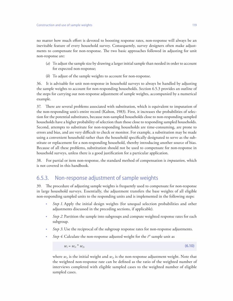
Construction and use of sample weights 119
no matter how much effort is devoted to boosting response rates, non‑response will always be an inevitable feature of every household survey. Consequently, survey designers often make adjust‑ments to compensate for non‑response. The two basic approaches followed in adjusting for unit non‑response are:
(a) To adjust the sample size by drawing a larger initial sample than needed in order to account for expected non‑response;
(b) To adjust of the sample weights to account for non‑response.
It is advisable for unit non‑response in household surveys to always be handled by adjusting 36. the sample weights to account for non‑responding households. Section 6.5.3 provides an outline of the steps for carrying out non‑response adjustment of sample weights, accompanied by a numerical example.
There are several problems associated with substitution, which is equivalent to imputation of 37. the non‑responding unit’s entire record (Kalton, 1983). First, it increases the probabilities of selec‑tion for the potential substitutes, because non‑sampled households close to non‑responding sampled households have a higher probability of selection than those close to responding sampled households. Second, attempts to substitute for non‑responding households are time‑consuming, are prone to errors and bias, and are very difficult to check or monitor. For example, a substitution may be made using a convenient household rather than the household specifically designated to serve as the sub‑stitute or replacement for a non‑responding household, thereby introducing another source of bias. Because of all these problems, substitution should not be used to compensate for non‑response in household surveys, unless there is a good justification for a particular application.
For partial or item non‑response, the standard method of compensation is 38. imputation, which is not covered in this handbook.
Non‑response adjustment of sample weights6.5.3. The procedure of adjusting sample weights is frequently used to compensate for non‑response 39.
in large household surveys. Essentially, the adjustment transfers the base weights of all eligible non‑responding sampled units to the responding units and is implemented in the following steps:
Step 1.• Apply the initial design weights (for unequal selection probabilities and other adjustments discussed in the preceding sections, if applicable).
Step 2.• Partition the sample into subgroups and compute weighted response rates for each subgroup.
Step 3• . Use the reciprocal of the subgroup response rates for non‑response adjustments.
Step 4.• Calculate the non‑response adjusted weight for the ith sample unit as
where w1i is the initial weight and w2i is the non‑response adjustment weight. Note that the weighted non‑response rate can be defined as the ratio of the weighted number of interviews completed with eligible sampled cases to the weighted number of eligible sampled cases.
wi = w1i * w2i (6.10)
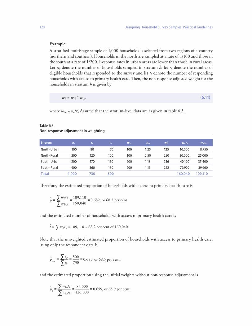
120 Designing Household Survey Samples: Practical Guidelines
Example
A stratified multistage sample of 1,000 households is selected from two regions of a country (northern and southern). Households in the north are sampled at a rate of 1/100 and those in the south at a rate of 1/200. Response rates in urban areas are lower than those in rural areas. Let nh denote the number of households sampled in stratum h, let rh denote the number of eligible households that responded to the survey and let th denote the number of responding households with access to primary health care. Then, the non‑response adjusted weight for the households in stratum h is given by
Table 6.3Non‑response adjustment in weighting
Stratum nh rh th w1h w2h wh wh rh wh th
North‑Urban 100 80 70 100 1.25 125 10,000 8,750
North‑Rural 300 120 100 100 2.50 250 30,000 25,000
South‑Urban 200 170 150 200 1.18 236 40,120 35,400
South‑Rural 400 360 180 200 1.11 222 79,920 39,960
Total 1,000 730 500 160,040 109,110
Therefore, the estimated proportion of households with access to primary health care is:
where w2h = nh/rh Assume that the stratum‑level data are as given in table 6.3.
wh = w1h * w2h (6.11)
pw tw rh h
h h
� = = =∑∑
109 110160 040
0 682,,
. , or 68.2 per cent
pw tw r
h h
h h
�1
1
1
83 000126 000
0 659= = =∑∑
,,
. , or 65.9 per cent.
ptruwh
h
� = = =∑∑
500730
0 685. , or 68.5 per cent,
t w th h� = =∑ 109 110, = 68.2 per cent of 160,040.
and the estimated number of households with access to primary health care is
Note that the unweighted estimated proportion of households with access to primary health care, using only the respondent data is
and the estimated proportion using the initial weights without non‑response adjustment is

Construction and use of sample weights 121
This example has been provided also for the purpose of illustrating how initial weights are 40. adjusted to compensate for non‑response. The results show considerable disparity between the esti‑mated proportion using only the initial weights and that using non‑response‑adjusted weights, but the difference between the unweighted proportion and the non‑response‑adjusted proportion appears to be negligible.
After non‑response adjustments of the weights, further adjustments can be made to the weights, 41. as appropriate. In the next section, adjustment of the weights to account for non‑coverage is con‑sidered.
Adjustment of sample weights for non‑coverage6.6. Non‑coverage refers to the failure of the sampling frame to cover all of the target population, 42.
with the result that some population units have no probability of selection for inclusion in the sample selected for the household survey. This is just one of many possible deficiencies of sampling frames used to select samples for surveys see chapter 4 for a detailed discussion of sampling frames.
Non‑coverage is a major concern for household surveys, especially those conducted in develop‑43. ing countries. Evidence of the impact of non‑coverage can be seen from the fact that sample estimates of population counts based on some developing‑country surveys fall significantly short of popula‑tion estimates from other sources. Therefore, the methodology of the identification, evaluation and control of non‑coverage in household surveys should be a key area of work and training in national statistical offices.
The present section discusses some sources of non‑coverage in household surveys and one of 44. the procedures used to compensate for non‑coverage, namely, statistical adjustment of the weights via post‑stratification.
Sources of non‑coverage in household surveys6.6.1. Most household surveys in developing countries are based on stratified multistage area prob‑45.
ability designs. The first‑stage units, or primary sampling units, are usually geographical area units. At the second stage, a list of households or dwelling units is created, from which the sample of households is selected. At the last stage, a list of house members or residents is created, from which the sample of persons is selected. Thus, non‑coverage may occur at any of three levels: the PSU level, the household level, and the person level.
Since PSUs are generally based on enumeration areas identified and used in a preceding popu‑46. lation and housing census, they are expected to cover the entire geographical extent of the target population. Thus, the size of PSU non‑coverage is generally small. For household surveys in develop‑ing countries, PSU non‑coverage is not as serious as non‑coverage at subsequent stages of the design. However, non‑coverage of PSUs does occur in most surveys. For instance, although a survey may be designed to provide estimates for the entire population in a country, or a region of the country, some PSUs may be excluded on purpose at the design stage, because some regions of a country are inaccessible owing to civil war or unrest, a natural disaster, or other factors. Also, remote areas with very few households or persons are sometimes removed from the sampling frames for household surveys because they are too costly to cover; as they represent a small proportion of the population, their effect on the population figures is very small (see chapter 4 for further discussion including

122 Designing Household Survey Samples: Practical Guidelines
numerous examples of non‑coverage of PSUs in household surveys). In the report of the results for such a survey, the exclusion of these areas must be explicitly indicated. The impression should not be created that survey results apply to the entire country or region when in fact a portion of the population is not covered. The non‑coverage properties of the survey must be fully indicated in the survey report.
Non‑coverage becomes a more serious problem at the household level. Most surveys consider 47. households to be a collection of persons who are usually related in some way and who usually reside in a dwelling or housing unit. There are important definitional issues to be resolved, such as who is to be considered a usual resident and what constitutes a dwelling unit. How are multi‑unit structures (such as apartment buildings) and dwelling units with multiple households to be handled? It may be easy to identify the dwelling unit, but complex social structures may make it difficult to identify the households within the dwelling unit. There is thus a lot of potential for misinterpretation or for inconsistent interpretation of these concepts by different interviewers, or in different countries or cultures. In any event, strict operational instructions are needed to guide interviewers on who is to be considered a household member and on what is to be considered a dwelling unit.
Other factors that contribute to non‑coverage include the inadvertent omission of dwelling 48. units from listings prepared during field operations, or of subpopulations of interest (for example, young children or the elderly), omissions due to errors in measurement, non‑inclusion of absent household members, and omissions due to the failure to properly understand survey concepts. There is also a temporal dimension to the problem, that is to say, dwelling units may be unoccupied or under construction at the time of listing, but may become occupied at the time of data col‑lection. For household surveys in developing countries, the non‑coverage problem is exacerbated by the fact that, for the most part, their censuses, the unique basis for constructing sampling frames, do not provide detailed addresses of sampling units at the household and person levels. Frequently, out‑of‑date or inaccurate administrative household listings are used, and individuals within a household are deliberately or accidentally omitted from a household listing of residents. More details on sources of non‑coverage are provided in Lepkowski (2003) and the references cited therein.
Compensating for non‑coverage in household surveys6.6.2. There exist several approaches to handling the problem of non‑coverage in household surveys 49.
(Lepkowski, 2003). These include:
(a) Improved field procedures such as the use of multiple frames and improved listing proce‑dures;
(b) Compensating for the non‑coverage through a statistical adjustment of the weights.
As regards the second approach, if reliable control totals are available for the entire population 50. and for specified subgroups of the population, one could attempt to adjust the weights of the sample units in such a way as to make the sum of weights match the control totals within the specified subgroups. The subgroups are termed post‑strata and the statistical adjustment procedure is called post‑stratification. This procedure compensates for non‑coverage by adjusting the weighted sampling distribution for certain variables so as to make it conform to a known population distribution (see Lehtonen and Pahkinen (1995) for some practical examples of how to analyse survey data with post‑stratification). A simple illustration is provided below.

Construction and use of sample weights 123
Example
Suppose that, in the preceding example, the number of households is known from an inde‑pendent source such as a current civil register to be 45,025 in the north and 115,800 in the south. Suppose further that the weighted sample totals are, respectively, 40,000 and 120,040. Carry out the following two steps:
Step 1• . Compute the post‑stratification factors.
For the northern region, we have: w h345 02540 000
1 126= =,,
. ; and
For the southern region, we have: w h3115 800120 040
0 965= =,,
. .
Step 2• . Compute the final, adjusted weight: wf = wh × w3h.
The numerical results are summarized in table 6.4.
Table 6.4Post‑stratified weighting for coverage adjustment
Stratum rh th wh wfh wfh rh wfh th
North‑Urban 80 70 125 140.75 11,260 9,852
North‑Rural 120 100 250 281.40 33,768 28,140
South‑Urban 170 150 236 227.77 38,721 34,166
South‑Rural 360 180 222 214.20 77,112 38,556
Total 730 500 160,861 110,714
The estimated proportion of households with access to primary health care is:
Note that with the weights adjusted by post‑stratification, the weighted sample counts 51. for the northern and southern regions are, respectively, 45,024 (11,256 + 33,768) and 115,821 (38,709 + 77,112), figures that closely match the independent control totals given above.
Increase in sampling variance due to weighting6.7. Even though the use of weights in the analysis of survey data tends to reduce the bias in the 52.
estimates, it could also inflate the variances of such estimates. To simplify the discussion, we consider a stratified single‑stage design with equal‑probability samples within strata. If the stratum variances (that is to say, the variances among units in the strata) are not the same in every stratum, then having unequal stratum weights across strata (for instance, weights inversely proportional to the stratum variances) might produce more precise survey estimates. However, if the stratum variances are the same in every stratum, then having unequal weights will lead to higher variances in the survey esti‑mates than those resulting from having equal weights.
pw tw rf
fh h
fh h
� = = =∑∑
110 714160 861
0 69,,
. , or 69 per cent.

124 Designing Household Survey Samples: Practical Guidelines
The effect of using weights is to increase the variance in an estimated population mean by the 53. factor
is the total realized sample size, wh is the final weight and nh is the realized sample size for stratum h. The above formula can also be written in terms of the coefficient of variation of the weights, as
L nn w
n w
h hh
h hh
= ×∑∑
2
2( ) (6.12)
where n nhh
= ∑
L n
w
wCV w
jj
jj
j= × = +∑∑
2
221
( )( ) (6.13)
where CV w nw
wn
w Variance of weigj
jj
j jjj
22
2 21( )( )
( )= −
=
∑ ∑∑ hhtsmean of weights( )
. 2
Therefore, L = × =730 1 0336,424,009160,861)2(
. .
Example
We now calculate the variance inflation factor using the data in the example in section 6.6.2, with final weights wfh and realized stratum sample sizes rh (see table 6.4).
Table 6.5Stratum parameters for variance
Stratum rh wfh wfh rh w 2fh rh
North‑urban 80 140.75 11,260 1,584,845
North‑rural 120 281.40 33,768 9,502,315
South‑urban 170 227.77 38,721 8,819,459
South‑rural 360 214.20 77,112 16,517,390
Total 730 160,861 36,424,009
In other words, there is an increase in variance in the survey estimates of about 3 per cent owing to the use of weights.
Trimming of weights6.8. Once the weights have been calculated and adjusted to compensate for the imperfections 54.
discussed above, it is advisable to examine the distribution of the adjusted weights. Extremely large weights, even if affecting only a small portion of sampled cases, can result in a substantial increase

Construction and use of sample weights 125
in the variance of survey estimates. Therefore, it is common practice to trim extreme weights to some maximum value in order to limit the associated variation in the weights (thereby reducing the variance of survey estimates) and at the same time prevent a small number of sampled units from dominating the overall estimate. Weight trimming is most frequently used after the adjustment of weights for non‑response.
While the trimming of weights tends to reduce the variance of estimates, it also introduces bias 55. in the estimators. In some instances, the reduction in variance due to the trimming of extremely large weights may more than offset the increase in the bias incurred, thereby reducing the mean‑squared error of the survey estimators. In practice, weight trimming should be carried out only when justi‑fied, that is to say, when it can be verified that the bias introduced due to the use of trimmed (as opposed to the original) weights has less impact on the total mean square error than the correspond‑ing reduction in variance achieved by trimming.
For any stratified design, the weight trimming process should ideally be carried out within 56. each stratum. The process starts with specifying an upper bound for the original weights and then adjusting the entire set of weights so that the sum of the trimmed weights is the same as that of the original weights. Let whi denote the final weight for the ith unit in stratum h, and let whB denote the upper bound for the weights specified for stratum h. Then, the trimmed weight for the ith sampled unit in stratum h can be defined as:
Now, the trimmed weights for the entire sample can be further adjusted so that their sum is 57. exactly the same as the sum of the original weights. For ease of exposition, we shall assume con‑stant weights within strata, and drop the subscript i for the rest of this discussion. Let FT denote the ratio of the sum of the original weights to the sum of the trimmed weights, in other words,
ww w ww w whi Thi hi hB
hB hi hB( ) =
<≥
if if
(6.14)
where the sums in the ratio are taken across all strata and hence over all units in the sample. If we define the adjusted trimmed weight for the hth stratum as
Fn w
n wT
h hh
h h Th
=∑
∑ ( ), (6.15)
The example offered below is designed to illustrate and aid understanding of the trimming procedure.
The first two columns of table 6.6 below give the total number of units and the final weight, 58. respectively, in each of seven strata. A maximum weight of 250 is chosen and so the original weights are truncated at 250, as shown in the third column of the table.
w F wh T Th T( )*
( ),= × (6.16)
then clearly, n w n wh h Th
h hh
( )* ,∑ ∑= as desired.

126 Designing Household Survey Samples: Practical Guidelines
Note that in this case,
Table 6.6Weight trimming
nh wh wh(T) nhwh nhwh(T) nhw*h(T)
80 140.75 140.75 11,260 11,260 11,823.00
100 150.25 150.25 15,025 15,025 15,776.25
125 175.00 175.00 21,875 21,875 22,968.75
150 200.00 200.00 30,000 30,000 31,500.00
120 250.00 250.00 30,000 30,000 31,500.00
120 275.13 250.00 33,015 30,000 31,500.00
170 285.40 250.00 48,518 42,500 44,625.00
Total 865 189,693 180,660 189,693.00
The trimmed weights have been rescaled so that they sum up to the original total 125 by multiplying each weight by FT =1.05.
Concluding remarks6.9. Sample weights have now come to be regarded as an integral part of the analysis of household 59.
survey data in developing countries, as in the rest of the world. Most survey programmes now advocate the use of weights even in the rare situations involving self‑weighting samples (in which case, the weights would be 1). In the past, tremendous efforts were expended by survey designers towards reaching the virtually unattainable goal of achieving self‑weighting samples and hence of making weights unnecessary in the analysis of survey data. The conventional wisdom was that the use of weights made the analyses too complicated and that there was very little, if any, computing infrastructure for weighted analysis. However, advances in computer technology in the past decade have invalidated this argument. Computer hardware and software are now affordable and available in many developing countries. In addition, many specialized computer software packages are now available specifically for the analysis of survey data. These are reviewed and compared in chapter 7.
As discussed, the use of weights reduces biases owing to imperfections in the sample related 60. to non‑coverage and non‑response. Non‑response and non‑coverage are different types of error due to the failure of a designed survey to obtain information from some units in the target popula‑tion. For household surveys in developing countries, non‑coverage is a more serious problem than non‑response. This chapter provided examples of procedures for developing and statistically adjust‑ing the basic weights to compensate for some of those household surveys‑related problems and for using the adjusted weights in the estimation of parameters of interest. The advent of fast‑speed computers and affordable or free statistical software should make the use of weights a routine aspect
Fn w
n wT
h hii
h hi Ti
= = =∑
∑ ( )
,,
. .189 693180 660
1 05

Construction and use of sample weights 127
of the analysis of household survey data even in developing countries. However, as this chapter has demonstrated, the development of sampling weights increases the complexity of survey operations in various ways. For example, weights need to be calculated for each stage of sample selection; they then need to be adjusted to account for various imperfections in the sample; and finally, they need to be stored and used appropriately in all subsequent analyses. Consequently, careful attention must be devoted to the development of weighting operations and the actual calculation of the weights to be used in the survey analysis.
References and further reading
Brick, J. M., and G. Kalton, (1996). Handling missing data in survey research. Statistical Methods in Medical Research, vol. 5, pp. 215‑238.
Cochran, W. G. (1977). Sampling Techniques, 3rd ed. New York: John Wiley & Sons.
Groves, R. M., and M. P. Couper, (1998). Non‑response in Household Interview Surveys. New York: John Wiley & Sons.
Groves, R. M., and others (2002). Survey Non‑response. New York:, John Wiley & Sons.
D. Kasprzyk, (1986). The treatment of missing survey data. Survey Methodology, vol. 12, pp. 1‑16.
Kalton, G. (1983). Compensating for Missing Survey Data. Ann Arbor, Michigan: Survey Research Center, University of Michigan.
Kish, L. (1965), Survey Sampling, New York: Wiley.
I. Hess, (1950). On non‑coverage of sample dwellings, Journal of the American Statistical Association, vol. 53, pp. 509‑524.
Lehtonen, R., and E. J. Pahkinen. (1995). Practical Methods for Design and Analysis of Complex Surveys, New York: Wiley.
Lepkowski, James. (2005), Non‑observation error in household surveys in developing countries. In Household Sample surveys in Developing and Transition Countries. Studies in Methods, No. 96. Sales No. E.05.XVII.6.
Lessler, J., and W. Kalsbeek, (1992). Nonsampling Error in Surveys,, New York: John Wiley & Sons.
Levy, P. S., and S. Lemeshow. (1999), Sampling of Populations: Methods and Applications, 3rd ed. New York: John Wiley & Sons.
Lohr, S. (1999), Sampling: Design and Analysis, Duxbury Press, Pacific Grove.
Yansaneh, I. S. (2004), Overview of Sample Design Issues for Household Surveys in Developing Countries, in Household Surveys in Developing and Transition Countries: Technical Report, United Nations, New York.


129
Chapter 7
Estimation of sampling errors for survey data
Introduction7.1.
The present chapter provides a brief overview of the various methods used for estimating sam‑1. pling errors for household survey data generated by various sample designs, ranging from standard designs that can be found in any introductory textbook on sampling theory (for example, Cochran (1977)), to more complex designs used for large‑scale household surveys. For the standard sample designs, formulae are provided along with numerical examples to illustrate the estimation of sam‑pling errors, the construction of confidence intervals, and the calculation of design effects and effec‑tive sample sizes. Sampling error estimation methods for more complex designs are then presented. The merits and demerits of each method are discussed and numerical examples are provided to illustrate the implementation of the procedures. An example is provided, based on data from a real survey, to illustrate the fact that standard statistical software packages underestimate the sampling errors of survey estimates, leading to wrong conclusions about the parameters of interest to the sur‑vey. To avoid this problem, the chapter strongly recommends the use of special statistical software packages that take full account of the complex nature of the designs commonly used for household surveys. Several of these software packages are described and compared.
Sampling error estimation for complex survey data7.1.1. The analytical objectives of well‑designed household surveys have in recent times moved beyond 2.
basic summary tables of counts or totals of parameters of interest. Analysts are now also interested in hypothesis‑generation and testing or model‑building. For instance, instead of simply estimating the proportion of a population in poverty or with secondary or higher education, analysts now want to evaluate the impact of policies, or explore the way in which a key response variable, for example, academic performance of a school‑going child, or the poverty level of a household, is affected by factors such as region, socio‑economic status, gender and age.
Answering these types of questions requires detailed analyses of data at the household or person 3. level. The publication of the results of such analyses must, of necessity, include appropriate measures of the precision or accuracy of the estimates derived from the survey data. Information on the preci‑sion of survey estimates is required for proper use and interpretation of survey results and also for

130 Designing Household Survey Samples: Practical Guidelines
the evaluation and improvement of sample designs and procedures. Such monitoring and evaluation of sample designs are particularly important in the case of large national survey programmes, which are frequently designed to be the only source of detailed information on a great variety of topics.
One of the key measures of precision in sample surveys is the sampling variance (the concept is 4. introduced in chapter 3), an indicator of the variability introduced by choosing a sample instead of enumerating the whole population, assuming that the information collected in the survey is correct. The sampling variance is a measure of the variability of the sampling distribution of an estimator. The standard error, or square root of the variance, is used to measure the sampling error. For any given survey, an estimator of this sampling error can be evaluated and used to indicate the accuracy of the estimates.
The form of the variance estimator, and how it is evaluated, depend on the underlying sample 5. design. For standard designs, these estimators are often evaluated by the use of simple formulae. However, for complex sample designs used for household surveys, which often involve stratification, clustering, and unequal probability sampling, the forms of these estimators are often complex and difficult to evaluate. The calculation of sampling errors in this instance requires procedures that take into account the complexity of the sample design that generated the data, which in turn often require the use of appropriate computer software.
In many developing countries, the analysis of household survey data is frequently restricted 6. to basic tabular analysis, with estimates of means, proportions and totals, but with no indication of the precision or accuracy of these estimates. Even in national statistical offices with an extensive infrastructure for statistical data collection and processing, one often finds a lack of expertise on detailed analysis of microlevel data. Some survey designers or analysts are often surprised to learn, for instance, that the clustering of elements introduces correlations among the elements that reduce the precision of the estimates relative to the simple random samples they are accustomed to analys‑ing; or that the use of weights in analysis generally inflates the sampling errors; or that the standard software packages they routinely use in their work do not appropriately account for these losses in precision.
This chapter attempts to remedy this situation by providing a brief overview of methods of com‑7. puting estimates of sampling error for the kinds of complex designs usually employed for household surveys in developing countries, as well as statistical software packages used in the analysis of such surveys. Several numerical examples are provided to illustrate the variance procedures discussed.
Overview7.1.2. Section 7.2 provides a first‑principle definition of sampling variance under simple random sam‑8.
pling, including numerical examples illustrating the calculation of sampling variance and the con‑struction of confidence intervals. Definitions of other measures of sampling error are provided in section 7.3. Section 7.4 provides formulae for the calculation of sampling variance under various standard designs, such as stratified sampling and cluster sampling. Several numerical examples are introduced to facilitate understanding of the concepts. Section 7.5 discusses common features of household survey designs, as well as the contents and structure of survey data required for appropriate estimation of sampling error. The general form of the estimates of interest in household surveys is also presented. Section 7.6 provides brief guidelines on the presentation of information on sampling errors and section 7.7 describes practical methods of calculating sampling errors under more complex

Estimation of sampling errors for survey data 131
designs. These methods frequently require special procedures and the use of specialized computer software packages. The pitfalls of using standard statistical software for the analysis of survey data are discussed in section 7.8, using an example based on data from an immunization coverage survey conducted in Burundi in 1989. Some publicly available software packages for sampling error estima‑tion for household survey data are reviewed and compared in sections 7.9 and 7.10. The chapter ends with some concluding remarks in Section 7.11.
Sampling variance under simple random sampling7.2. The sampling variance of an estimate can be defined as the average squared deviation about 9.
the average value of the estimate, where the average is taken across all possible samples. As indi‑cated in chapter 3, simple random sampling is the most elementary of sampling techniques, but it is rarely used in large‑scale surveys because its implementation is very inefficient and prohibitively expensive.
To facilitate understanding of the concept of sampling variance, we consider a small popula‑10. tion of five households (N=5), from which a small sample of two households (size n=2) is selected by simple random sampling without replacement (SRSWOR). Suppose that the variable of interest is the monthly household expenditure on food, and that the expenditures of each of the four households are as given in Table 7.1 below:
Table 7.1Monthly expenditure in dollars on food per household
Household (1) Expenditure on food in dollars (Y1)
1 10
2 20
3 30
4 40
5 50
First, note that since we know the value of the variable of interest for all the households in 11. our population, we can calculate the value of the parameter corresponding to the average monthly household expenditure on food, that is to say,
The SRSWOR estimator for the average monthly expenditure on food is
YN
Yii
N= = + + + + = =
=∑1 10 20 30 40 50
5150
530
1.
where the summation is taken over the units selected into the sample. Clearly, the estimate obtained depends on the sample selected. Table 7.2 below shows all possible samples, the estimate based on each sample, the deviations of each sample estimate from the population mean, and the squared
Y Yii S
� = ∑12 ε
,

132 Designing Household Survey Samples: Practical Guidelines
Note that the average of the estimates based on all possible samples is
Table 7.2Calculating the true sampling variance of Y , the parameter for the average
Sample 1 Sample units Sample estimate (Yi) Yi – Yave (Yi – Yave)2
1 (1, 2) 15 –15 225
2 (1, 3) 20 –10 100
3 (1, 4) 25 –5 25
4 (1, 5) 30 0 0
5 (2, 3) 25 –5 25
6 (2, 4) 30 0 0
7 (2, 5) 35 5 25
8 (3, 4) 35 5 25
9 (3, 5) 40 10 100
10 (4, 5) 45 15 225
Average 30 0 750
deviations. Note that Y ave� denotes the average of all the sample‑based estimates. Note that Y is the
symbol for population mean while Y� is the symbol for the estimate of the population mean called the sample mean (see table 7.2).
In other words, the average value of the estimate across all possible samples is equal to the 12. population average. An estimate with such a property is termed as unbiased for the parameter that it is estimating.
The true sampling variance of the estimated average monthly expenditures on food from an 13. SRSWOR of size n=2 from this population is
Y Yave ii
� �= = + + + + + + + + + = ==∑1
1015 20 25 30 25 30 35 35 40 45
1030010
31
1000 =Y .
The problem with the above approach stems from the fact that it is not practical to select all 14. possible samples from the population. In practice, only one sample is selected, and the population values are not known. A more practical approach is to use formulae for calculating variance. Such formulae exist for all standard sample designs.
Under simple random sampling without replacement, the sampling variance of an estimated 15. mean (Y�), based on a sample of size n, is given by the expression
Var Y Y Yii
ave( ) ( ) .� � �= − = ==∑1
1075010
751
102
Var Y nN n
( ) .� = −
12δ (7.1)

Estimation of sampling errors for survey data 133
is a measure of the variability of the characteristic of interest (population variance of Y ). Usually, δ 2 is unknown and must be estimated from the sample (see equation 7.2 below). It can be clearly seen from the above formula that the sampling variance depends on the following factors:
(a) Population variance of the characteristic of interest;
(b) Size of the population;
(c) Sample size;
(d) Sample design and method of estimation.
The proportion of the population that is in the sample, 16. n/N, is called the sampling fraction (denoted by f ); and the factor [1–(n/N)], or 1–f, which is the proportion of the population not included in the sample, is called the finite population correction factor ( fpc). The fpc represents the adjustment made to the standard error of the estimate to account for the fact that the sample is selected without replacement from a finite population. Note, however, that when the sampling fraction is small, the fpc can be ignored. In practice, the fpc can be ignored if it does not exceed 5 per cent (Cochran, 1977).
The above formula indicates that the sampling variance is inversely proportional to the sample 17. size. As the sample size increases, the sampling variance decreases; and for a census or complete enu‑meration (where n=N), there is no sampling variance. Note that non‑response effectively decreases the sample size and so increases sampling variability.
It can be shown that an unbiased estimate of the sampling variance of the estimated mean is 18. given by
Where δ 2
2
1
1=
−
−=∑( )Y Y
N
ii
N �
v Y nN
sn
( ) ( )� = −12
(7.2)
Y v Y� �±1 96. ( ). (7.3)
P number of units with characteristicn
� = (7.4)
and v P nN
P Pn
( ) ( ) ( ) .� � �= − −
−1 1
1 (7.5)
where 138 is an estimate of the population variance, δ 2 , based on the sample. This is referred to as the sample variance. The 95 per cent confidence interval for the population mean (see para. 30, chapter 3) is given by
For a population proportion, the sample‑based estimate and estimated variance are given, 19. respectively, by

134 Designing Household Survey Samples: Practical Guidelines
Table 7.3 below summarizes the estimates of various population quantities and the variances 20. of the estimates under simple random sampling without replacement.
In general, the 21. ( )1−α per cent confidence interval for the population mean is given by
Table 7.3Estimates and their variances for selected population characteristics
Parameter Estimate Variance of estimate
Population mean (Y�) Yn
Yii Sample
� = ∑1
εv Y n
Nsn
( ) ( )� = −12
Population total T NY� �= v T N v Y( ) ( )� �= 2
Population proportion for a category P number of sampled units in category
n� =
v P nN
P Pn
( ) ( ) ( )� � �= − −
−1 1
1
where z1 2−α / is the ( / )1 2− −α th percentile of the standard normal distribution.
The following example illustrates the estimation of sampling variance based on a selected 22. sample.
Example 1
Consider a simple random sample of n = 20 households drawn from a large population of N=20,000 households. The data collected are presented in table 7.4 below, where the variable Y denotes weekly household expenditure on food and the variable Z indicates whether or not a household possesses a television set (z=1 if yes, and 0 otherwise).
Estimate z estimated variance of estimate± −1 2α / (7.6)
Table 7.4Weekly household expenditure on food and TV ownership for sampled households
Household (i) Yi Zi i Yi Zi
1 5 0 11 7 1
2 10 1 12 8 1
3 5 0 13 9 1
4 9 1 14 10 1
5 5 1 15 8 1
6 6 1 16 8 0
7 7 0 17 5 0
8 15 1 18 7 0
9 12 1 19 12 1
10 8 0 20 4 0
Total 160 12

Estimation of sampling errors for survey data 135
The estimate of the population mean monthly household expenditure on food is
The estimated variance of the estimated mean is
The 95 per cent confidence interval for the population mean is
The estimate of the population total monthly household expenditure on food is
The estimated variance of the estimated total is
The 95 per cent confidence interval for the population mean is
The estimate of the population proportion of households that possess a TV is
The estimated variance of the estimated proportion of the households with TV is
The 95 per cent confidence interval for the population mean is
Y Yii
� = = + + + + = ==∑1
205 10 12 4
2016020
81
20 ... .
v Y( ) (,
) ( ) ( ) ..... ( ) ( )� = − − + − + + − + −
1 2020 000
5 8 10 8 12 8 4 819
2 2 2 2 = 7 87. .
8 1 96 7 87± ×. . = (2.50, 13.50).
Y NY� �= = × =20 000 8 160 000, , .
0 6 1 96 0 0126. . .± × = (0.38, 0.82).
v P( ) (,
) . ( . )� = − −1 2020 000
0 6 1 0 619
= 0.0126.
P Zii
� = = ==∑1
201220
0 61
20. .
160 000 1 96 3 148 000 000, . , , ,± × = (50,030, 269,970).
v Y( ) , . , , , .� = × =20 000 7 87 3 148 000 0002

136 Designing Household Survey Samples: Practical Guidelines
Other measures of sampling error7.3. In addition to sampling variance, there are other measures of sampling error. These include the 23.
standard error, the coefficient of variation, and the design effect. These measures are algebraically related in the sense that it is possible to derive the expression of any one of the measures from the others using simple algebraic operations.
Standard error7.3.1. The standard error of an estimator is the square root of its sampling variance. This measure 24.
is easier to interpret since it provides an indication of sampling error using the same scale as the estimate, whereas the variance is based on squared differences.
A question that frequently arises in the design of surveys is how large a standard error is to be 25. considered acceptable. The answer to this question depends on the magnitude of the estimate. For example, a standard error of 100 would be considered small when estimating annual income but large when estimating the average weight of people. Also, the standard error of 3 148 000 000, , , = 56,107 for the estimated total of 160,000 obtained in example 1 above can be considered too large.
Coefficient of variation7.3.2. The coefficient of variation (CV) of an estimate is the ratio of its standard error to the average 26.
value of the estimate itself. Thus, the CV provides a measure of the sampling error relative to the characteristic being measured. It is usually expressed as a percentage.
The CV is useful in comparing the precision of survey estimates whose sizes or scales differ. 27. However, it is not useful for estimators of characteristics whose true value can be zero or negative, including estimates of change, for example, change in average income over two years.
Design effect7.3.3. The design effect (denoted as 28. deff ) is defined as the ratio of the sampling variance of an estima‑
tor under a given design to the sampling variance of the estimator based on a simple random sample of the same size. It can be thought of as the factor by which the variance of an estimate based on a simple random sample of the same size must be multiplied to take account of the complexities of the actual sample design due to such factors as stratification, clustering and weighting.
In other words, an estimator based on data from a complex sample of size 29. n has the same variance as the estimator computed from data from a simple random sample of size n/deff. For this reason, the ratio n/deff is sometimes called the effective sample size for estimation based on data from a complex design. For a general discussion of “effective sample size” calculations, see Kish (1995) and Potthoff, Woodbury and Manton (1992) and references cited therein. Also, see various sections of chapter 3 for a more detailed discussion of design effects and their use in sample design.
Calculating sampling variance for other standard designs7.4. For simple designs and simple linear estimates such as means, proportions and totals, it is usu‑30.
ally possible to derive formulae that can be used to calculate variances of estimates. However, for the kinds of complex designs and estimates associated with household surveys, this is often difficult

Estimation of sampling errors for survey data 137
or impossible. In the present section, we provide examples to illustrate the calculation of sampling variance for stratified and single‑stage cluster sample designs. Formulae and examples of variance calculations for other standard sample designs are provided in textbooks (for example, Cochran, 1977; and Kish, 1965).
Stratified sampling7.4.1. A detailed description of stratified sampling is provided in chapter 3 and annex I. In 31.
this section, we shall concern ourselves only with the estimation of variance under the design. Consider a stratified design with H strata, with sample estimates of population means for the strata given by Y Y YH1 2, , ... ... , and sample estimates of the population variances for the strata given by S S SH1
222 2, . , ... ... An estimator of the population mean under this design is
where Y h� is the sample‑based estimate of Y h Hh , , ... ... . =1 The variance of the estimator is given by
With stratified random sampling, the estimator and its estimated variance are given by
where yh is the sample mean for stratum h, Nh is the population size in stratum h, and
The estimated variance of this estimate under stratified random sampling is given by
Y Yst hh
H� �==∑
1, (7.7)
v Y v Yst hh
H( ) ( ).� �=
=∑
1 (7.8)
Y NN
y W ysth
hh
H
h hh
H� = == =∑ ∑
1 1, (7.9)
W NN
h Hhh= =, , ... ... . 1
v Y W v y NN
nN
sn
st h hh
Hh
h
Hh
h
h
h( ) ( ) ( ) ,� = =
−= =∑ ∑2
1 1
2 21 (7.10)
where nh is the sample size in stratum h, and sh2 is the sample variance, a sample‑based estimate of S h Hh
2 1, , ... ... . =
Example 2
We now apply these results to an example of a stratified design involving three strata with parameters as given in table 7.5 below. Suppose that we are interested in estimating the popula‑tion mean, based on an overall sample of size 1,500.

138 Designing Household Survey Samples: Practical Guidelines
The estimate of the population mean is
Table 7.5Example of data for a stratified sample design
Parameter PopulationStratum 1 (capital city)
Stratum 2 (province‑urban)
Stratum 3 (province‑urban)
Size N = 1,000,000 N1 = 300,000 N2 = 500,000 N3 = 200,000
Variance S 2 = 75,000 S 21 = ? S 2
2 = ? S 23 = ?
Mean Y = ? Y1 = ? Y2 = ? Y3 = ?
Cost per unit N/A C1=1 C2=4 C3=16
Sample size under optimal allocationa n = 1,500 n1 = 857 n2 = 595 n3 = 48
Sample mean N/A y1 = 4,000 y2 = 2,500 y3 = 1,000
Sample variance N/A s 21 = 90,000 s 2
2 = 62,500 s 23 = 10,000
Note: N/A signifies not applicable.a See chapter 3.
The estimated variance of the above estimate is
Y st� = × + × +300 000
1 000 0004 000 500 000
1 000 0002 500 200 000,
, ,, ,
, ,, ,
11 000 0001 000 2 650
, ,, , .× =
The 95 per cent confidence interval for the population mean is
v Y st( ) ,, , ,
,� =
−
300 0001 000 000
1 857300 000
90 000857
2
+
−
500 0001 000 000
1 595500 000
62 500595
2,, , ,
,
+
−
200 0001 000 000
1 48200 000
10 00048
2,, , ,
,
= 43 98516. .
Note that the estimated variance of the estimated mean under simple random sampling is given by
2 650 1 96 43 98516 2 637 2 663, . . ( , , , ).± × =
Therefore, the design effect of this stratified design is 43 9851649 925
0 88..
.= and the effective sample size is
v Y SRS( ) ( ,, ,
) ,,
. .� = − × =1 1 5001 000 000
75 0001 500
49 925
1 5000 88
1 705,.
, .=
This means that the estimate based on a stratified random sample of size 1,500 has the same variance as that based on a simple random sample of size 1,705.

Estimation of sampling errors for survey data 139
A detailed description of the cluster sampling technique is provided in chapter 3. In the present 32. section, we provide a simple example to illustrate the calculation of sampling errors for the special case of single‑stage cluster sampling.
Example 3
Suppose that we are interested in estimating the proportion of school‑age children in a province that have been immunized against polio myehtis. Assume, for simplicity’s sake, that there are a total of 500 equal‑sized enumeration areas (EAs) in the province, each with 25 school‑age children. The EAs serve as the clusters in this example. Suppose that we select 10 EAs by sim‑ple random sampling without replacement out of the 500 EAs in the province and that the proportion of immunized school‑aged children is measured for each sampled EA, with the results as shown in table 7.6 below.
Table 7.6Proportions of immunized school‑age children in 10 enumeration areas as the variable of interest
Sampled EA (i) 1 2 3 4 5 6 7 8 9 10
Sample proportion (P̂i)8
251025
1225
1425
1525
1725
2025
2025
2125
2325
For this example, the estimate of the proportion of immunized school‑age children in the province is
Furthermore, the sample variance is
P� = =160250
0 64. , or 64 per cent.
Therefore, the variance of the estimated proportion is
s P PP ii
2
1
1021
10 10 040533=
−− =
=∑( ) .� � .
Note that under simple random sampling, the estimated variance of the estimated proportion is
v P( ) ( ) . . .� = − × =1 10500
0 04053310
0 003972
This means that the estimate based on the cluster sample of size 250 has the same variance as that based on an a simple random sample of size 57.
v PSRS( ) (,
) . ( . ) . .� = − × −−
=1 25012 500
0 64 1 0 64250 1
0 0009078
Therefore, the design effect for this cluster sample design is 0 0039720 0009078
..
= 4.38
and the effective sample size is 2504 38
57.
.=

140 Designing Household Survey Samples: Practical Guidelines
Common features of household survey sample 7.5. designs and dataDeviations of household survey designs from simple random sampling7.5.1.
As earlier stated, simple random sampling is rarely used in practice for large‑scale household 33. surveys because they are too expensive to implement. However, a thorough understanding of this design is important because it forms the theoretical basis for more complex sample designs. Most sample designs for household surveys deviate from simple random sampling owing to the presence of one or more of the following three features:
(a) Stratification at one or more stages of sampling;
(b) Clustering of units in one or more stages of sampling, which reduces costs but inflates the variance of estimates owing to the correlations among the units in the same cluster;
(c) Weighting to compensate for such sample imperfections as unequal probabilities of selec‑tion, non‑response and non‑coverage (see chapter 6 for details).
A sample design is referred to as 34. complex if it has one or more of the above features. Most household survey designs are complex and thus violate the assumptions of simple random sampling. Therefore, analysing household survey data as if they were generated by a simple random sample design would lead to errors in the analysis and in the inferences based on such data. Furthermore, as already mentioned, the estimates of interest in most household surveys cannot be expressed as linear functions of the observations so that there may not be any closed‑form formulae for the variances. The following sections address the issue of variance estimation methods for household survey designs that take into account the complexities outlined above.
Preparation of data files for analysis7.5.2. Survey data collected in developing countries are sometimes not amenable to analysis that 35.
extends beyond basic frequencies and tabulations. There are several reasons for this. First, there may be very limited or no technical documentation of the sample design for the survey. Second, the data files may not have the format, the structure and the requisite information that would allow any sophisticated analysis. Third, there may be a lack of the appropriate computer software and techni‑cal expertise.
In order for sample survey data to be analysed appropriately, the associated database must 36. contain all the information reflecting the sample selection process (see chapter 5 for a detailed discussion). In particular, the database should include appropriate labels for the sample design strata, the primary sampling units (PSUs), secondary sampling units (SSUs), etc. Sometimes, the actual strata and PSUs used in selecting the sample for a survey need to be modified for purposes of variance estimation. Such modifications are necessary to make the actual sample design fit into one of the sample design options available in at least one of the statistical analysis software pack‑ages (see section 7.9). The strata and PSUs created for variance estimation are sometimes called pseudo‑strata, or variance strata and pseudo‑PSUs or variance PSUs. The relevant sample design variables, as well as the variables created for variance estimation purposes, should be included in the data file, along with corresponding documentation on how these variables are defined and used. A minimum set of three variables is required for variance estimation: the sample weight,

Estimation of sampling errors for survey data 141
the stratum (or pseudo‑stratum) and the PSU (or pseudo‑PSU). These three variables summarize the sample design, and their inclusion in the survey data set allows the appropriate analysis of the data, accounting for the complexities in the sample design.
Furthermore, sample weights should be developed for each sampling unit in the data file. These 37. weights should reflect the probability of selection of each sampling unit as well as compensate for survey non‑response and other deficiencies in the sample. The sample weights and the labels for the design variables are required for the appropriate estimation of the variability of the survey estimates. As mentioned in chapter 6 and in the preceding sections of this chapter, sample weights are impor‑tant not only for generating appropriate survey estimates, but also for estimating of the sampling errors of those estimates. Therefore, it is essential that all information on weights be incorporated into the data files. In particular, whenever non‑response, post‑stratification or other types of adjustments are made, the survey documentation must contain a description of these adjustment procedures.
Types of survey estimates7.5.3. For most household surveys, the most common survey estimates of interest are in the form 38.
of totals and ratios. Assume a stratified three‑stage design with PSUs at the first stage, SSUs at the second stage and households at the third stage. The survey estimate of a total can be expressed as
Where Whijk = the final weight for the kth household (k = 1, … … 1j) selected in the j th SSU ( j = 1, … … mi) in the ith PSU (i = 1, … … nh) in hth stratum (h = 1, … … H); and
Yhijk = the value of the variable Y for the kth household selected in the jth SSU in the ith PSU in the hth stratum.
At the most basic level, the weights associated with the sample units are inversely proportional 39. to the probabilities of selection of the units into the sample. However, more sophisticated methods are often used to compute the weights to be applied in the analysis. Some of these methods are described in chapter 6 and in the references cited therein.
The survey estimate of a ratio is defined as40.
Y W Yhijkk
l
j
m
i
n
h
H
hijk
jih� =
====∑∑∑∑
1111, (7.11)
where Y� and X� are estimates of totals for variables Y and X, respectively, calculated as specified in equation (7.12) above.
In the case of multistage sampling, means and proportions are just special cases of the ratio 41. estimator. In the case of the mean, the variable X, in the denominator of the ratio, is a count vari‑able, defined to equal 1 for each element so that the denominator is the sum of the weights. In the case of a proportion, the variable X in the denominator is also defined to equal 1 for all elements; and the variable Y, in the numerator, is a binomial variable, defined to equal either 0 or 1, depend‑ing on whether or not the unit observed possesses the characteristic whose proportion is being
R YX
� ��= , (7.12)

142 Designing Household Survey Samples: Practical Guidelines
estimated. In most household surveys, the denominator in the ratio estimator is variously defined as total population, total females, total males, total rural population, total population in a given province or district, etc.
Guidelines for presentation of information 7.6. on sampling errorsDetermining what to report7.6.1.
For large‑scale national surveys with numerous variables and domains of interest and several, 42. often competing objectives, it is not practical to present each and every estimate along with its associated sampling error. Not only will this drastically increase the volume of the publication, but it is also likely to clutter the presentation of substantive results. In light of the expected variability in the sampling error estimates themselves, presenting the results for too many individual variables may lead to confusion and a perception of inconsistency regarding the overall quality of the survey data collected. It is much more useful to present sampling error information for a few of the most important characteristics of interest upfront, while relegating the rest to an appendix.
In presenting information on sampling errors, it is important to keep in mind its potential 43. impact on the interpretation of the results of the survey and policy decisions that may derive from such interpretation. Sampling error information should always be viewed as just one component of total survey error, and not always the most significant one. In some survey situations, nonsampling errors (see chapter 8) might have a more significant impact than sampling errors might on the overall quality of the survey data. For this reason, it is recommended that the information on sampling errors include a discussion of the main sources of non‑sampling errors and some qualitative assessments of the impact on the overall quality of the survey data. Since sampling errors become more critically important at lower levels of disaggregation, it is also recommended that some cautionary remarks be included on the degree to which the survey data may be disaggregated.
In general, information on sampling errors should include enough detail to facilitate correct 44. interpretation of the survey results, and to satisfy the requirements of the entire spectrum of data users, ranging from the general data user or policymaker (whose interest is in using the survey results to formulate policy) and the substantive analyst who is (engaged in further analysis and reporting of the results) to the sampling statistician (who is concerned with the statistical efficiency of the design compared with other alternatives, and with features of the design that might be used in designing future surveys).
How to report sampling error information7.6.2. Sampling errors may be presented in three different forms, as:45.
(a) Absolute values of standard errors;
(b) Relative standard errors (square roots of relative variances);
(c) Confidence intervals.
The choice among these three forms of presentation depends on the nature of the estimate. 46. In situations where the estimates vary in size and units of measurement, the same value of standard

Estimation of sampling errors for survey data 143
errors may be applicable to the estimates when expressed in relative terms; consequently, it would be more efficient to present relative standard errors. However, in general, absolute standard errors are much easier to understand and to relate to the estimate, especially in the case of percentages, proportions and rates. Using confidence intervals requires a choice of confidence level (say, 90, 95 imposed or 99 per cent). Since this varies according to survey objectives and the precision require‑ments on the estimates, it is important to specify the confidence level being used in the presentation of sampling error information and to then retain this confidence level throughout in determining the significance of the results. As earlier stated the interval most frequently used in practice is the 95 per cent confidence interval (see paras.30 and 22 in chapters 3 and 7 respectively), that is to say:
For more details on the subject of presentation of information on sampling errors, including 47. specific guidelines for various categories of users and a number of illustrations, see United Nations (1993) and the references cited therein.
Rule of thumb in reporting standard errors7.6.3. A frequently used rule of thumb in reporting standard errors is to report the standard error 48.
to two significant digits and then report the corresponding point estimate to the same number of decimal places as the standard error. For example:
1. If the point estimate is 73,456 with standard error of 2,345, then we report the point estimate as 73,500 and the standard error as 2,300.
2. If the point estimate is 1.54328 with standard error of 0.01356, then we report the point estimate as 1.543 and the standard error as 0.014.
The general reasoning behind this rule of thumb appears to be related to t‑statistics. The pres‑49. ence of two significant digits in the standard error and the corresponding number of digits in the point estimate ensures that there is not too much of a rounding error effect in the resulting t‑statistics and, at the same time removes the implication of an excessive level of precision given by point esti‑mates reported to a large number of irrelevant digits. Note, however, that this rule of thumb does not necessarily work in settings where t‑statistics are not of primary interest.
Methods of variance estimation for household surveys7.7. In the present section, we briefly describe some conventional methods for estimating variances 50.
or sampling errors for estimates based on survey data. Methods for the estimation of sampling errors for household surveys can be classified into four broad categories:
(a) Exact methods;
(b) Ultimate cluster method;
(c) Linearization approximations;
(d) Replication techniques.
We shall now briefly discuss each of these in turn. Interested readers can obtain more details from such references as Kish and Frankel (1974), Wolter (1985) and Lehtonen and Pahkinen (1995).
Estimate Standard Error± ×1 96. (7.13)

144 Designing Household Survey Samples: Practical Guidelines
Exact methods7.7.1. Sections 7.2 and 7.4 provided several examples of exact methods of variance estimation for 51.
standard sample designs. These methods constitute the best approach to variance estimation when they are applicable. However, their application to the calculation of sampling variances of estimates based on household survey data is complicated by several factors. First, sample designs used for most household surveys are more complex than simple random sampling (see section 7.5.1 above). Second, the estimates of interest might not be in the form of simple linear functions of the observed values, and so the sampling variance can frequently not be expressed in a closed‑form formula, like that of the sample mean under simple random sampling or under stratified sampling. Furthermore, exact methods depend on the sample design under consideration in a particular application, the estimate of interest, and the weighting procedures used.
In the following sections, we discuss methods of variance estimation for sample designs usu‑52. ally employed for household surveys. These methods are designed to overcome the shortcomings of the exact methods.
Ultimate cluster method7.7.2. The ultimate cluster method of variance estimation see (Hansen, Hurwitz and Madow, 1953, 53.
pp. 257‑259) can be used to estimate the variances of survey estimates based on a sample generated by a complex sample design. Under this method, the ultimate cluster consists of the entire sample from a PSU, regardless of sampling at subsequent stages of the multistage design. Variance estimates are computed using only between‑PSU totals without having to compute variance components at each stage of selection.
Suppose a sample of 54. nh PSUs are selected from stratum h (with any number of stages within PSUs). Then the estimate of the total for stratum h is given by
Note that PSU‑level estimate Y hi� is an estimate of Ynh
h
�. Thus, the variance of the individual PSU‑level
estimates is given by
Y Yh hii
nh� �=
=∑
1, (7.14)
where Y W Yhi hijkj
m
hijk
i� =
=∑
1.
and the variance of their total, Y h� , the stratum‑level total, estimated from a random sample of size nh estimator of the population total for stratum h, is given by
v Yn
Y Yn
hih
hih
hi
nh( ) .� � �
=−
−
=∑1
1 1
2
(7.15)
v Y nn
Y Yn
hh
hhi
h
hi
nh( ) .� � �
=−
−
=∑1 1
2
(7.16)

Estimation of sampling errors for survey data 145
Note that simple algebraic manipulation yields the following equivalent expression for the 55. variance estimator of the population total for stratum h
Finally, with independent sampling across strata, the variance estimator for the overall popula‑56. tion total is obtained by taking the sum of the variances of the stratum‑level totals, that is, to say,
v Y nn
YY
nh
h
hhi
hii
n
hi
n
h
h
( )� ��
=−
−
=
=
∑∑1
2 1
2
1.. (7.17)
Note that sometimes a finite population correction factor (1–nh/Nh) is used in the above formulae.
Equation (7.18) is remarkable in the sense that the variance of the estimated total is a function 57. of the appropriately weighted PSU totals Y hi� only, without any reference to the structure and man‑ner of sampling within PSUs. This considerably simplifies the variance estimation formula because the computation of variance components attributable to the other stages of sampling within PSUs is not required. This feature affords the ultimate cluster method great flexibility in handling differ‑ent sample designs and is, indeed, one of the method’s major strengths and a major reason for its widespread use in survey work.
Now, the variance estimator of the ratio, 58. R YX
� ��= , is given by
v Y v Y hh
H( ) ( ).� �=
=∑
1 (7.18)
where v Y( )� and v X( )� are calculated according to the formula for the variance of an estimated total, and
v RX
v Y R v X Y X( ) ( ) ( ) cov( , ) ,��
� � � � �= + −{ }1 222
(7.19)
or, equivalently,
cov( , )Y X nn
X Xn
Y Yn
h
hhi
h
hhi
h
hi
nh� � � � � �
=−
−
−
=∑1 1
=∑h
H
1, (7.20)
Note that the above formula for the variance of a ratio can be simplified by using the fact that 59. the relative variance of the ratio is approximately equal to the difference between the relative vari‑
cov( , )Y X nn
X YX Y
h
hhi hi
hii
n
hii
nh h
� � � �� �
=−
−
= =∑ ∑
11 1
nnhi
nh
=∑
1. (7.21)

146 Designing Household Survey Samples: Practical Guidelines
ances of the numerator and the denominator. Recall that the relative variance of an estimator is the ratio of its variance to its square. Thus, for an estimated ratio R�, the relative variance, denoted by relvar (R�), is given by
Therefore an estimate of the variance of the ratio is given by
relvar R v R
R ( ) ( )� �
�= 2 (7.22)
The ultimate cluster method of calculating sampling errors for estimated totals and ratios could 60. be schematized in the following steps:
Step 1• . For each stratum separately, compute the weighted estimate Y hi� for the character‑istic of interest, Y, for each PSU (in accordance with the weighting procedures specified in chapter 6).
Step 2• . Calculate the squared value of each estimated PSU value from step 1.
Step 3• . Calculate the sum of the values from step 2 over all PSUs in the stratum.
Step 4• . Calculate the sum of the estimated PSU totals from step 1 over all PSUs.
Step 5• . Square the result of step 4 and divide by nh, the number of PSUs in the stratum.
Step 6• . Subtract the result of step 5 from that of step 3, and multiply this difference by the factor nh/(nh–1). This is the estimated variance for the characteristic at the stratum level.
Step 7• . Sum the result of Step 6 over all strata to obtain the overall estimated variance for the characteristic of interest.
Step 8• . Calculate the square root of the result of step 7 to obtain the estimated sampling error for the characteristic of interest.
To calculate the estimated sampling error for ratios, such as estimated proportions, we proceed 61. as follows:
Step 9• . Calculate the relative variance of the numerator, Y�, by dividing the result of step 7 by the square of the estimate of the numerator.
Step 10• . Repeat step 9 to obtain the relative variance of the denominator, X�.
Step 11• . Subtract the result of step 10 from that of step 9.
Step 12• . Multiply the result of step 11 by the square of the estimated ratio, R�. This is the estimated variance of R�.
Step 13• . Calculate the square root of the result of step 12 to obtain the estimated sampling error for R�.
Example 4
We now consider a hypothetical example to illustrate the ultimate cluster method of variance estimation. Suppose that we are interested in estimating the total weekly expenditure on food for households in city A. We design a survey employing a stratified three‑stage clustered design involving three strata with two PSUs selected from each stratum and two households selected
v R R R R Y X ( ) ( ) ( ) ( ) .� � � � � �= = −{ }2 2relvar relvar relvar (7.23)

Estimation of sampling errors for survey data 147
from each sampled PSU. The weekly expenditure on food is then recorded for each sampled household in the survey. Table 7.7 presents the data obtained from such a survey, including the weights (Whij) and weekly expenditure on food, in dollars (Yhij), for each sampled household.
Table 7.7Weekly household expenditure on food, by stratum
Stratum PSU Household Weight (Whij) Expenditure, in dollars (Yhij) Whij*Yhij
11
1 1 30 302 1 28 28
21 3 12 362 3 15 45
21
1 5 6 302 5 7 35
21 2 16 322 2 18 36
31
1 6 7 422 6 8 48
21 4 13 522 4 15 60
Total 42 474
Pursuant to chapter 6, an estimate of the total household weekly expenditure on food for the 62. city is here given by
Also, an estimate of the average household weekly expenditure on food is given by
Y W Yhij hijjih
� = ====∑∑∑
1
2
1
2
1
3474.
We now implement the steps in the ultimate cluster method of variance estimation in the 63. columns of Table 7.8 below. The column numbers correspond to the steps outlined above.
Y
W Y
W
hij hijjih
hijjih
� = = ====
===
∑∑∑
∑∑∑1
2
1
2
1
3
1
2
1
2
1
347442
11 (to the nearest dollar).
Table 7.8Implementing the steps in the ultimate cluster method of variance estimation
Stratum PSU Step 1 Step 2 Step 3 Step 4 Step 5 Step 6 Step 7
11 58 3,364 9,925 139 9,660.5 5292 81 6,561 – – –
21 65 4,225 8,849 133 8,844.5 92 68 4,624 – – –
31 90 8,100 20,644 202 20,402 4842 112 12,544 – – –
Total 1, 022

148 Designing Household Survey Samples: Practical Guidelines
The stratum‑level variance estimates are 529 for stratum 1, 9 for stratum 2, and 484 for 64. stratum 3. The overall estimate of variance for the estimated total weekly household income (step 7 in our scheme) is obtained by adding together the stratum‑level estimates, whose sum is 1,022.
Linearization approximations7.7.3. Most estimates of interest in household surveys are non‑linear. Some examples are the average 65.
body mass index of school‑age children in a country, the proportion of income spent on housing costs in a given city, the ratio of the odds of a population subset’s having a characteristic to that of another subpopulation’s having the same characteristic, etc. In the linearization method, such non‑linear estimates are “linearized” using a Taylor series expansion. This involves expressing the estimate in terms of a Taylor series expansion and then approximating the variance of the estimate by the variance of the first‑order or linear part of that expansion using the exact methods discussed in earlier sections.
Suppose that we wish to estimate the variance of an estimate 66. z of a parameter Z and suppose z is a non‑linear function of simple estimates y1, y2, … … ym of parameters Y1, Y2, … … Ym. that is to say,
Assuming that z is close to Z, the Taylor series expansion of z to terms of the first degree in z–Z is
z = f (y1, y2, … … ym). (7.24)
where d’i is the partial derivatives of z with respect to the y’i, that is to say,
z Z d y Yii
m
i i= + −=∑
1( ) (7.25)
which is a function of the basic estimate yi. This means that the variance of z can be approximated by the variance of the linear function in equation (7.24) above, which we know how to calculate from the exact methods presented in preceding sections that is to say,
d zyii
= ∂∂
,
Equation (7.26) involves an 67. m × m covariance matrix of m basic estimates y1, y2, … … ym, with m variance terms and m (m–1)/2 identical covariance terms, which can be evaluated from the exact methods for linear statistics discussed in earlier sections.
Example 5 (variance of a ratio)
To illustrate the linearization approach, we consider the estimation of variance for the ratio
v z v d y d v y d d y yi i ii
m
i ii j
j i j( ) ( ) ( ) cov( , ).= = +∑ ∑ ∑= ≠
2
1 (7.26)
z r yx
= = . (7.27)

Estimation of sampling errors for survey data 149
Note that for this case, ∂∂
= ∂∂
= − = −ry x
rx
yx
rx
12 and . Therefore,
which is the familiar expression for the variance of a ratio found in most sampling textbooks.
Linearization is widely used in practice because it may be applied to almost all sample designs 68. and to any statistic that can be linearized, that is to say, expressed as a linear function of familiar statistics such as means or totals, with coefficients coming from partial derivatives required in the Taylor series expansion. Once linearized, the variance of the non‑linear estimate can be approxi‑mated using the exact methods described above (see Cochran (1977) and Lohr (1999) for technical details about the linearization process including examples).
Advantages7.7.3.1.
Because the linearization method of variance estimation has been in use for a long time, its 69. theory is well developed, and it is applicable to a wider class of sampling designs than that to which replication methods are applicable (described below). If the partial derivatives are known, and quad‑ratic and higher‑order terms in the Taylor series expansion are of negligible size, then linearization produces an approximate variance estimate for almost all linear estimators of interest, such as ratios and regression coefficients.
Limitations7.7.3.2.
Linearization works well only if the above assumptions about partial derivatives and high‑70. er‑order terms are correct. Otherwise, serious biases in the estimates may result. Also, it is generally difficult to apply the method to complex functions involving weights. A separate formula must be developed for each type of estimator, and this can require special programming. The method can‑not be applied to statistics such as the median and other percentiles that are not smooth functions of population totals or means.
Furthermore, it is difficult to apply non‑response and non‑coverage adjustments with the lin‑71. earization approach, which depends on the sample design, the estimate of interest, and the weighting procedures. It also requires that the sample design information (strata, PSUs, weights) be included in the data file.
Replication7.7.4. The replication approach encompasses to a class of methods that involve the taking of repeated 72.
subsamples, or replicates, from the data, re‑computing the weighted survey estimate for each replicate, and the full sample, and then computing the variance as a function of the deviations of these replicate estimates from the full‑sample estimate. The approach can be summarized in the following steps:
Step 1• . Delete different subsamples from the full sample to form replicate samples.
Step 2.• Produce replicate weights by repeating the estimation process for each replicate sample.
Step 3.• Produce an estimate from the full sample and from each set of replicate weights.
v rx
v y r v x r y x( ) ( ) ( ) cov( , ) ,= + −{ }1 222 (7.28)

150 Designing Household Survey Samples: Practical Guidelines
Step 4.• Compute the variance of the estimate as of the squared deviations of the replicate estimates from the full‑sample estimate.
For instance, suppose that 73. k replicates are created from a sample, each with estimates θ θ θ� � �1 2, , ... ... k of a parameter θ , and suppose that the estimate based on the full sample is θ�0. Then the replication‑based estimate of the variance is given by
where c is a constant, that depends on the estimation method. Replication methods differ in respect of the value of the constant and in manner in which the replicates are formed (see section 7.7.5 for a brief review of the most commonly used replication techniques).
Data file structure7.7.4.1.
Whatever the replication technique, the data file structure remains the same as, shown in 74. table 7.9 below.
Advantages7.7.4.2.
The main advantage of the replication approach relative to the linearization approach is that 75. replication uses the same basic estimation method regardless of the statistic being estimated (because the variance estimate is a function of the sample, not of the estimate), whereas a linearization approximation must be developed analytically for each statistic, a potentially laborious exercise in large household surveys with large numbers of characteristics of interest. Furthermore, replication techniques are convenient to use and are applicable to almost all statistics, linear or non‑linear. With replication, estimates can be easily computed for subpopulations and the effects of non‑response and other adjustments can be reflected in the replicate weights.
Limitations7.7.4.3.
Replication techniques are computer‑intensive, mainly because they require the computation 76. of a set of replicate weights, which are the analysis weights, recalculated for each of the replicates selected so that each replicate appropriately represents the same population as the full sample. Also,
var ( ) ( ) , θ θ θ� � �= −=∑1
01
2
cr
r
k (7.29)
Table 7.9Data file structure for the replication approach.
Record Data
Full sample weight
Replicate weights
1 2 3 … k
1 Data 1 w1 w11 0 w13 … w1k
2 Data 2 w2 0 w22 w23 … w2k
3 Data 3 w3 w31 w32 0 … w3k
… … … … … … … …
… … … … … … … …
… … … … … … … …
N Data n wn wn1 wn2 wn3 … 0
Note: Dotes indicate series

Estimation of sampling errors for survey data 151
the formation of replicates may be complicated by restrictions in the sample design (see section 7.7.5 below), which can sometimes lead to the overestimation of sampling errors.
We conclude our general comparison of linearization and replication approaches to sampling error 77. estimation by noting that the two approaches do not produce identical estimates of sampling error. However, empirical investigations (see Kish and Frankel, 1974) have shown that, for large samples and many statistics, the differences between the results produced by these two methods are negligible.
Some replication techniques7.7.5. The most commonly used replication techniques are:78.
(a) Random groups;
(b) Balanced repeated replication (BRR);
(c) Jackknife replication (JK1, JK2, and JKn);
(d) Bootstrap.
We now briefly discuss each of these techniques in turn.
Random groups7.7.5.1.
The random group technique entails dividing the full sample into 79. k groups in such a way as to preserve the survey design, that is to say, each group represents a miniature version of the survey, mirroring the sample design. For instance, if the full sample is an SRS of size n, then the random groups can be formed by randomly apportioning the n observations into k groups, each of size n/k. If it is a cluster sample, then the PSUs are randomly divided among the k groups, in such a way as to ensure that each PSU retains all its observations, hence each random group is still a cluster sample. If the sample is a stratified multistage sample, then random groups can be formed by selecting a sample of PSUs from each stratum. Note that the total number of random groups to be formed in this instance cannot exceed the number of sampled PSUs in the smallest stratum.
The random group method can be easily used to estimate sampling errors for both linear 80. statistics such as means and totals and smooth functions thereof, and nonlinear ones such as ratios and percentiles. No special software is necessary for estimating the sampling error, which is simply the standard deviation of the estimates based on the random groups formed from the full sample. However, creating the random groups can be difficult in complex sample designs, since each random group must preserve the design structure of the complete survey. Furthermore, the number of ran‑dom groups may be limited by the survey design itself. For instance, for a design with two PSUs per stratum, only two random groups can be formed and, in general, a small number of random groups leads to imprecise estimates of sampling error. A general rule of thumb is to have at least 10 random groups in order to obtain a more stable estimate of sampling error.
Balanced repeated replication7.7.5.2.
Balanced repeated replication (BRR) assumes a design with two PSUs per stratum. Forming a 81. replicate involves dividing each stratum into two PSUs, and selecting one of the two PSUs in each stratum, according to a prescribed pattern, to represent the entire stratum. The technique can be adapted to other designs by grouping the PSUs into pseudo‑strata, each with two PSUs.

152 Designing Household Survey Samples: Practical Guidelines
Jackknife7.7.5.3.
Like the BRR, the Jackknife is a generalization of the random group method that allows the 82. replicate groups to overlap. There are three types of Jackknife: the JK1, the JK2 and the JKn tech‑niques.
The JK1 is the typical drop‑one‑unit Jackknife for SRS designs. However, it can be used for 83. other designs if the sampled units are grouped into random subsets, each of which resembles the full sample.
The JK2 is similar to the BRR in the sense that it assumes a two‑PSU per stratum design. In 84. case of self‑representing PSUs, pairs of secondary sampling units (SSUs) can be created. Like the BRR, the JK2 can be adapted to other designs by the grouping of PSUs into pseudo‑strata, each with two PSUs. One PSU is then dropped at random from each stratum in turn in order to form the replicates.
The JKn is the typical drop‑one‑unit Jackknife for stratified designs. To create replicates, each 85. PSU is dropped in turn from each stratum. The remaining PSUs in the stratum are re weighted to estimate the stratum total. The number of replicates is equal to the number of PSUs (or pseu‑do‑PSUs).
Bootstrap7.7.5.4.
The Bootstrap technique starts with the selection of the full sample that reproduces all the 86. important features of the whole population. The full sample is then treated as if it were the whole population, and subsamples are drawn from it. As before, the estimate of sampling error is obtained by taking the standard deviation of the estimates based on the resamples from that based on the full sample.
The Bootstrap method works well for general sample designs and for non‑smooth functions 87. such as percentiles. However, it requires more computations than do the other replication tech‑niques.
Table 7.11 below, specifies in the value of the constant c in the variance formula (equation 88. (7.28)) that corresponds to the various replication methods.
Example 6 (Jackknife)
We now give a simple numerical example applying the Jackknife method of variance estima‑tion. Suppose we have a sample of size 3. We can create 3 subsamples each of size 2 by drop‑
Table 7.10Values of the constant factor in the variance formula for various replication techniques
Replication technique Value of constant c in equation (7.28)
Random group k(k–1)
BRR k
JK1 1
JK2 2
JKn k/(k–1)
Bootstrap k–1

Estimation of sampling errors for survey data 153
ping one unit at a time from the full sample. Table 7.11 below presents the values of a variable (Y ). For the three subsamples, an “X” indicates which units of the sample are included in the subsample.
Table 7.11Applying the jackknife method of variance estimation to a small sample and its subsamples
Subsample (g)
Sample unit Y 1 2 31 5 X X2 7 X X3 9 X XSample total 21Sample mean 7 6 7 8
The Jackknife variance estimate of the sample mean is given by
Sample variance: s22 25 7 7 7 9 7
3 14
2
= − + − + −−
=( ) ( ) ( ) .
Estimate of variance of sample mean (ignoring fpc): sn
2 43
= .
Mean of subsample means: y y y1 2 3
36 7 8
37
+ + = + + = .
which is exactly the same as the estimated variance of the sample mean, calculated above.
Example 7 (formation of replicates)
Table 7.12 uses the data in example 4 (section 7.7.2) to illustrate the formation of replicate samples for various replication methods and also the calculation of variances by the Jackknife method.
V y nn
y yJ gg
( ) ( ) ( ) ( ) ( ) ,= − − = − − + − + − ==∑1 3 1
36 7 7 7 8 7 4
31
32 2 2 2
Table 7.12Full sample: expenditure by stratum
Stratum PSU Household Weight Whij Expenditure Yhij Whij*Yhij
1 1 1 1 30 301 1 2 1 28 281 2 1 3 12 361 2 2 3 15 452 1 1 5 6 302 1 2 5 7 352 2 1 2 16 322 2 2 2 18 363 1 1 6 7 423 1 2 6 8 483 2 1 4 13 523 2 2 4 15 60Total 42 474

154 Designing Household Survey Samples: Practical Guidelines
Estimated mean based on full sample = = = ====
===
∑∑∑
∑∑∑Y
W Y
W
hij hijjih
hijjih
�0
1
2
1
2
1
3
1
2
1
2
1
347442
11.
Table 7.13Jackknife method (drop PSU 2 from stratum 1)
Stratum PSU Household Weight (Whij) Expenditure (Yhij) Whij*Yhij
1 1 1 1 30 301 1 2 1 28 282 1 1 5 6 302 1 2 5 7 352 2 1 2 16 322 2 2 2 18 363 1 1 6 7 423 1 2 6 8 483 2 1 4 13 523 2 2 4 15 60Total 42 474
We can continue this process, dropping one PSU at a time from each stratum. A total of six replicate samples can be formed in this way. Table 7.14 below shows the estimates of mean weekly household income based on each of the six replicate samples.
Estimated mean based on the above replicate sample = = =Y�139336
11.
Table 7.14Replicate‑based estimates
Replicate j PSU deleted Estimate
1 PSU 2, stratum 1 11 0 0
2 PSU 1, stratum 1 10 –1 1
3 PSU 2, stratum 2 10 –1 1
4 PSU 1, stratum 2 12 1 1
5 PSU 2, stratum 3 12 1 1
6 PSU 1, stratum 3 13 2 4
Total 8
The Jackknife estimate of the variance of the estimated mean is given by
var ( ) ( ) .JKh
hj
j
n
h
HY n
nY Y
h� � �= − −
= × =
==∑∑ 1 1
28 40
2
11
(Note that for this example, H=3 and nh=2 for all h.)

Estimation of sampling errors for survey data 155
We conclude this section by giving another example of the formation of replicate samples using 89. the balance repeated replication method. The results shown in table 7.15 below are for the pattern of deletions of PSUs specified in the table title.
Pitfalls of using standard statistical software packages 7.8. to analyse household survey data
Appropriate analyses of household survey data require that sampling errors of estimates be 90. computed in a manner that takes into account the complexity of the design that generated the data. This includes stratification, clustering, unequal‑probability sampling, non‑response, and other adjust‑ments of sample weights (see chapter 6 for details on the development and adjustment of weights). Standard statistical software packages do not account for these complexities because they typically assume that the sample elements were selected from the population by simple random sampling. As demonstrated in chapter 6, point estimates of population parameters are impacted by the sample weights associated with each observation. These weights depend upon the selection probabilities and other survey design features such as stratification and clustering. When they ignore the sample weights, standard packages yield biased point estimates. Performing a weighted analysis with these packages reduces the bias in the point estimates somewhat, but even then, the sampling errors of point estimates are often grossly underestimated because the variance estimation procedure typically does not take into account other design features such as stratification and clustering. This means that inferences drawn from such analyses would be misleading. For instance, differences between groups might be erroneously declared significant or hypotheses might be erroneously rejected. Wrong inferences from the analyses of household data could, for instance, have significant implication for resource allocation and policy formulation at the national and regional levels.
We now use an example from Brogan (2004) to illustrate the fact that the use of standard 91. statistical software packages can lead to biased point estimates, inappropriate standard errors and confidence intervals, and misleading tests of significance. The example is based on a data set from a tetanus toxoid (TT) immunization coverage sample survey conducted in Burundi in 1989. One of the objectives of the survey was to compare seropositivity (defined as a tetanus antitoxin titre of at least 0.01 international units/milliliter (IU/ml) with history of tetanus toxoid vaccinations. For
Table 7.15Balanced repeated replication method (Drop PSU 2 From Strata 1 and 3; PSU 1 from stratum 2)
Stratum PSU Household Weight Whij Expenditure Yhij Whij*Yhij
1 1 1 1 30 30
1 1 2 1 28 28
2 2 1 2 16 32
2 2 2 2 18 36
3 1 1 6 7 42
3 1 2 6 8 48
Total 18 216
Estimated mean based on the above BRR sample = = =Y BRR�
121618
12, .

156 Designing Household Survey Samples: Practical Guidelines
more information on this survey’s methodology and its published results, see Brogan (2004) and the references cited therein. Table 7.16 below presents estimates of the percentage of women who were seropositive and the associated standard error and confidence interval.
Note that the point estimates are the same for all programmes that use weights, but there is 92. a clear difference between the weighted and unweighted estimates. Furthermore, standard errors produced by the appropriate software are nearly twice that produced by standard software packages that assume simple random sampling. In other words, the standard software packages seriously underestimate the variances of survey estimates. This could have important implications for policy. For instance, if some intervention was being planned based on a proportion of seropositivity of 65 per cent or less, then such intervention would be implemented as a result of the analysis based on the special software packages, but might not be implemented on the basis of analysis using standard software packages. Table 7.16 reveals that the software packages that appropriately estimate the vari‑ances of survey estimates produce approximately the same results. In the next section, we provide a brief overview of some publicly available statistical software packages that are used for the analysis of household survey data.
Computer software for sampling error estimation7.9. The above methods of sampling error estimation have been in use for a long time in devel‑93.
oped countries, implemented mainly by customized computer algorithms developed by government statistical agencies, academic institutions, and private survey organizations. Recent advances in computer technology have led to the development of several software packages for implementing these techniques. Many of these software packages are now available for use on personal computers. The software packages use only one of the general approaches to variance estimation discussed in section 7.7. Most of these software packages produce the most widely used estimates, such as means, proportions, ratios, and linear regression coefficients. Some software packages also include approxi‑mations for a wide range of estimators, such as logistic regression coefficients.
In the present section, we present a brief overview of some publicly available software for the 94. estimation of sampling errors for household survey data. This is by no means an exhaustive list of all available programmes and packages. We restrict attention to a few statistical software packages that are currently available on personal computers for use by the general survey data analyst. Each software package is briefly reviewed, specifying the applicable sample designs and variance estima‑
Table 7.16Using various software packages to estimate the variances of survey estimates, with the proportion of women who were seropositive among women with recent birth, Burundi, 1988‑1989
Software Package Percentage seropositive Standard error 95 per cent confidence Interval
SAS 8.2 means without weights 74.9 2.1 (70.8, 79.0)
SAS 8.2 means with weights 67.2 2.3 (62.7, 71.7)
SAS 8.2 survey means 67.2 4.3 (58.8, 75.6)
SUDAAN 8.0 67.2 4.3 (58.8, 75.6)
STATA 7.0 67.2 4.3 (58.8, 75.6)
EPI INFO 6.04d 67.2 4.3 (58.8, 75.6)
WESVAR 4.1 67.2 4.3 (58.8, 75.6)

Estimation of sampling errors for survey data 157
tion methods. The advantages and disadvantages of using the software are also highlighted. No attempt is made to detail the technical and computational procedures underlying the packages. Such information can be obtained from the websites of the packages and from some of the references cited at the end of this chapter.
The six packages reviewed here are CENVAR, EPI INFO, PC CARP, STATA, SUDAAN and 95. WESVAR. SUDAAN (Shah, Barnwell and Bieler, 1998), STATA (StataCorp, 1996), PC CARP (Fuller and others, 1989), and CENVAR all use the linearization method for estimating the sam‑pling errors for non‑linear statistics. WESVAR uses replication methods only. Recent versions of SUDAAN also implement BRR and Jackknife techniques. Also, SAS and SPSS (which are not reviewed here) have developed new modules for the analysis of survey data. The replication‑based programs offer many of the basic methods, except the Bootstrap. We provide only a brief compari‑son of the general features of these software packages. A thorough comparison would require more extensive comparisons across sample surveys of different sizes and far more statistics, which are beyond the scope of the limited review conducted here.
Internet links to the several statistical software packages reviewed in this chapter, and to many 96. others, can be found at the following website: www.fas.harvard.edu/~stats/survey‑soft/survey‑soft.html.
Brogan (2004) provides a detailed comparison of several statistical software packages, includ‑97. ing the ones reviewed here, based on data from the Burundi household survey mentioned above.
We now provide brief overviews of the software packages. Interested readers can obtain more 98. details from the current manuals or from the websites indicated below.
CENVARUnited Stats Bureau of the Census; contact International Programs CenterUnited States Bureau of the CensusWashington, D.C. 20233‑8860E‑mail: [email protected]: www.census.gov/ipc/www/imps
CENVAR is a component of a statistical software system designed by the United States Bureau 99. of the Census for processing, management and analysis of complex survey data, namely, the Inte‑grated Microcomputer Processing System (IMPS). It is applicable to most sample designs, such as simple random sampling, stratified random sampling, and multistage cluster sampling. CENVAR uses linearization approximation for variance estimation.
Estimates produced by CENVAR include means, proportions and totals for the total sample 100. as well as specified subclasses in a tabular layout. In addition to the sampling error, the 95 per cent confidence interval limits, coefficients of variation, design effects, and unweighted sample sizes are provided.
EPI INFOUnited States Centers for Disease Control and PreventionEpidemiology Program Office, Mailstop C08Centers for Disease Control and PreventionAtlanta, GA 30333E‑mail: [email protected]: http://www.cdc.gov/epiinfo/

158 Designing Household Survey Samples: Practical Guidelines
EPI INFO is a statistical software system designed by the United States Centers for Disease 101. Control and Prevention for processing, managing and analysing epidemiological data, including complex survey data (CSAMPLE component). Relevant documentation is available online in the program and can be printed chapter by chapter. It is designed specifically for stratified multistage cluster sampling through the ultimate cluster sampling model.
EPI INFO produces sampling error estimates for means and proportions for the total sam‑102. ple as well as for subclasses specified in a two‑way layout. The printed output includes unweighted frequencies, weighted proportions or means, standard errors, 95 per cent confidence interval limits, and design effects.
PC CARPIowa State UniversityStatistical Laboratory219 Snedecor HallAmes, IA 50011Website: http://cssm.iastate.edu/software/pccarp.html
PC CARP is a statistical software package developed at Iowa State University for the estima‑103. tion of standard errors for means, proportions, quantiles, ratios, differences of ratios, and analysis of two‑way contingency tables. The program is designed to handle stratified multistage cluster samples. PC CARP uses the linearization approach for variance estimation.
STATAStata Corporation702 University Drive EastCollege Station, TX 77840E‑mail: [email protected]: http://www.stata.com
STATA is a statistical analysis software package designed for the estimation of sampling 104. errors for means, totals, ratios, proportions, linear regression, logistic regression, and probit analysis procedures. Additional capabilities include the estimation of linear combinations of parameters and hypothesis tests, as well as the estimation of quantiles, contingency table analysis, missing data compensation, and other analyses. STATA uses the linearization approach for variance estimation.
SUDAANResearch Triangle InstituteStatistical Software CenterResearch Triangle Institute3040 Cornwallis RoadResearch Triangle Park, NC 27709‑2194E‑mail: [email protected]: http://www.rti.org/patents/sudaan.html
SUDAAN is a statistical software package for analysis of correlated data, including complex 105. survey data. It is applicable to a wide variety of designs, including simple random sampling and multistage stratified designs. It provides facilities for estimation of a range of statistics and their asso‑ciated sampling errors, including means, proportions, ratios, quantiles, cross‑tabulations, and odds

Estimation of sampling errors for survey data 159
ratios; linear, logistic and proportional hazards regression models; and contingency table analysis. The program uses the linearization approach for variance estimation.
WESVARWestat, Inc.1650 Research Blvd.Rockville, MD 20850‑3129E‑mail: [email protected]: http://www.westat.com/wesvar/
WESVAR is a statistical software system designed by Westat, Inc., for the analysis of complex 106. survey data, including contingency table analysis, regression, and logistic regression. It is applicable to most sample designs but is specifically designed for stratified multistage cluster samples based on the ultimate cluster sampling model.
WESVAR uses replication techniques for variance estimation, including Jackknife, balanced 107. half sample, and the Fay modification to the balanced half sample method. It requires that a new version of the data set be created in a special WESVAR format and the specification of replicate weights.
General comparison of software packages7.10. The software packages reviewed here have many features in common. All programs require 108.
the specification of weights, strata, and sampling units for each sample element. They do not all handle every conceivable sample design in an unbiased fashion. For example, primary sampling units in most stratified multistage sample designs are selected with probabilities proportionate to size and without replacement. Only one program in the list, SUDAAN, has features designed to handle explicitly this type of design. However, all listed programs will handle such a design under an ultimate cluster sample selection model (see section 7.7 above). Furthermore, SUDAAN also has features designed to estimate variances for designs employing without‑replacement selection of primary sampling units. STATA is the only package with estimation features to account for the stratification and multistage selection employed in the design.
All of the packages estimate sampling variances and related statistics (design effects, intra‑class 109. correlation, etc.) for means, totals and proportions for the total sample, for subclasses of the total sample, and for differences between subclasses. Most of them estimate sampling variances for regres‑sion and logistic regression statistics. All of them estimate test statistics based on the sampling vari‑ances they produce.
CENVAR, EPI INFO, PC CARP, and WESVAR are available either for free, or at a nominal 110. charge. Interested users should use the e‑mail addresses and other contact information provided to obtain further information on how to acquire the software and associated documentation.
Concluding remarks7.11. This chapter has presented a brief overview of procedures for calculating sampling errors of 111.
estimates based on both standard sample designs and more complex designs used for household sur‑veys. The calculation of sampling errors is a critically important aspect of the analysis and reporting

160 Designing Household Survey Samples: Practical Guidelines
of results derived from household surveys. Ideally, sampling errors should be calculated for all char‑acteristics in the tabulation package of the survey. In practice, however, a set of key characteristics of interest is designated for the calculation of sampling errors for each domain. The characteristics cho‑sen should be those regarded as substantively important to the survey, but they should also include a representative choice of items that have certain statistical properties, namely, those thought to be highly clustered (for example, variables indicating ethnicity or access to services); and those thought to have low clustering effects (such as marital status). In addition, the choice should be guided by other features, such as characteristics encompassing a high or low proportion of the population, or important domains of interest.
This chapter has also advocated the use of special computer software for the estimation of 112. sampling errors for survey data. We have provided examples of situations in which serious errors are committed in the estimation of sampling errors when standard statistical software packages are used. In general, the use of standard statistical packages for household survey data analysis will understate the true variability of the survey estimates. These smaller estimates of standard error can lead to the drawing of misleading conclusions regarding the results of the survey, evaluating, for instance, erroneously declaring significant differences between the means of two groups or incorrectly reject‑ing a hypothesis.
The chapter has also provided a catalogue of some publicly available statistical software pack‑113. ages, along with basic contact information and an overview of their application. The lack of knowledge or expertise in sampling error estimation is one of the impediments to the conduct of sophisticated analysis of data in developing countries. Many analysts are not aware of the need to use specialized software or, if they are aware, prefer not undertake training in the use of a new software package.
It must be emphasized that the chapter represents only an introduction to the vast and grow‑114. ing field of variance estimation for complex survey data. The reader is encouraged to examine some of the references cited at the end of the chapter for a more detailed and systematic treatment of the subject. For a more extensive review of these and other software packages, including computer code and output for some of the available software, see Brogan (2004) and the references cited therein.
Finally, it must be recognized that with rapid advances in technology, many software packages 115. in a relatively short time either become obsolete or are improved beyond the specifications provided in this review. Indeed, it is possible that some of the specifications will be obsolete by the time this handbook is published. It is therefore important to remember that at the time of their use, the most accurate information regarding the software packages should be obtained from their respective manuals or websites.
References and further reading
An, A., and D. Watts (2001). New SAS procedures for analysis of sample survey data. SUGI Paper, No. 23, Cary, North Carolina: SAS Institute, Inc. Available from http://support.sas.com/rnd/app/papers/survey.pdf..
Binder D. A. (1983). On the variances of asymptotically normal estimators from complex surveys, International Statistical Review, Vol. 51, pp. 279‑92.
Brick J. M., and others J. (1996), A User’s Guide to WesVarPC, Rockville, Maryland: Westat, Inc..
Brogan, Donna (2005). Sampling error estimation for survey data. Household Sample on Surveys in Developing and Transition Countries. In Studies in Methods, No. 96. Sales No. E.05.XVII.6.
Estimation of sampling errors for survey data 161
Burt, V. L., and S. B. Cohen (1984). A comparison of alternative variance estimation strategies for complex survey data. Proceedings of the American Statistical Association Survey Research Methods Section:
Carlson, B. L., A. E. Johnson and S.B. Cohen (1993). An Evaluation of the Use of Personal Computers for Variance Estimation with Complex Survey Data, Journal of Official Statistics 9, No. 4, pp. 795‑814
Dippo, C.S ., R. E. Fay and D.H. Morganstein (1984). Computing variances from complex samples with replicate weights. Proceedings of the American Statistical Association Survey Research Methods Section.
Fuller, Wayne, and others (1989). PC CARP: USERS MANUAL, Ames, Iowa: Statistics Laboratory, Iowa State University. Available from http://cssm.lastate.edu/software.
Hansen, M. H., W. N. Hurwitz and W.G. Madow (1953). Sample Survey Methods and Theory, Vol. I, Methods and Applications. New York: Wiley, Sect. 10.16.
Hansen M.H., W.G. Madow and B.J. Tepping (1983). An evaluation of model‑dependent and probability‑sampling inferences in sample surveys. Journal of the American Statistical Association vol. 78, No. 384, pp. 776‑793
Kist, Leslie (1965). Survey Sampling. New York: John Wiley and sons.
________ (1995). Leslie Kish: Selected Papers, Steven Heeringa and Graham Kalton, eds. Hoboken, New Jersey: John Wiley & sons, Inc.
Kish, L., and M. R. Frankel (1974). Inference from complex samples. Journal of the Royal Statistical Society: services B, vol. 36, pp. 1‑37
Landis J. R., and others (1982). A statistical methodology for analyzing data from a complex survey: the First National Health and Nutrition Examination Survey. Vital and Health Statistics, vol. 2, No. 92., Washington, D.C.: Department of Health, Education and Welfare.
Lehtonen, R., and E. J. Pahkinen (1995). Practical Methods for Design and Analysis of Complex Surveys. New York: Wiley
Lepkowski J. M., J. A. Bromberg and J. R. Landis (1981), A program for the analysis of multivariate categorical data from Complex Sample Surveys. Proceedings of the American Statistical Association Statistical Computing Section.
Levy, Paul S., and Stanley Lemeshow (1999). Sampling of Populations: Methods and Applications. 3rd ed. New York: John Wiley & Sons.
Lohr, Sharon (1999). Sampling: Design and Analysis. Pacific Grove, California: Duxbury Press.
Potthoff, R. F., M. A. Woodbury and K.G. Manton, (1992). “Equivalent sample size” and “equivalent degrees of freedom” refinements for inference using survey weights under superpopulation models. Journal of the American Statistical Association, vol. 87, pp. 383‑396.
Rust K. (1985), “Variance Estimation for Complex Estimators in Sample Surveys,” Journal of Official Statistics 1(4), 381‑397.
Rust, K. F., and J. N. K. Rao (1996). Variance estimation for complex surveys using replication techniques”, Statistical Methods in Medical Research, vol. 5, pp. 283‑310
Shah, Babhai V. (1998) Linearization methods of variance estimation. In Encyclopedia of Biostatistics, vol. 3, Peter Armitage and Theodore Colton, eds. New York: John Wiley and sons, pp. 2276‑2279.

162 Designing Household Survey Samples: Practical Guidelines
Shah B. V., B. G. Barnwell and G. S. Bieler, (1996). SUDAAN User’s Manual: Release 7.0,, Research Triangle Park, North Carolina: Research Triangle Institute.
Tepping B. J. (1968), Variance estimation in complex surveys, Proceedings of the American Statistical Association Social Statistics Section, pp. 11‑18.
United Nations (1993). Sampling errors in household surveys. UNFPA/UN/INT‑92‑P80‑15E. New York: Statistical Division, Department for Economic and Social Information and Policy Analysis, and National Household Survey Capability Programme.
Wolter, K. M. (1985), Introduction to Variance Estimation. New York: Springer‑Verlag.
Woodruff, R. S. (1971), A simple method for approximating the variance of a complicated estimate. Journal of the American Statistical Association, vol. 66, No. 334, pp. 411‑414

163
Chapter 8
Non‑sampling errors in household surveys
Introduction8.1.
Both sampling errors and 1. non‑sampling errors need to be controlled and reduced to a level at which their presence does not defeat the usefulness of the final survey results. In the preceding chapters on sample design and estimation methodology, much attention was focused on sampling error and some‑what less on other sources of variation in surveys, such as non‑response and non coverage, which make up the class of errors known collectively as non‑sampling errors. Non‑sampling errors are particularly harmful when they are non‑random, because of the bias they introduce in survey estimates.
All survey data are subject to error from various sources. The broad, fundamental distinction is 2. between errors arising in the measurement process and sampling errors, that is to say, errors in the estimation of population values arising from measurement of a sample of the population.
In the preceding chapters, it was assumed that each unit 3. Yi in a population was associated with a value yi deemed the true value of the unit for characteristic y. Also assumed was that whenever Yi was in the sample, the value of y reported or observed on it is yi. This will hold in some, but not all situations. For example, in countries with a viable and comprehensive registration of vital events through birth certificates, “true” values may be easily obtainable when yi denotes age. However, in other situations, such as that involving a qualitative assessment of one’s health, true values may be much harder to obtain or even define. For example a sick person may rate him/herself fit depending on the circumstances.
In survey practice the supposition that the value reported or observed on unit 4. Yi is always yi, irre‑spective of who reports it or under what circumstances it is obtained, is unwarranted. Actual survey experience provides numerous examples that show errors of measurement or observation, as well as errors from erroneous response, non‑response and other causes whenever a survey is carried out.
In addition to response errors, surveys are subject to errors of coverage, processing, etc. The 5. quality of a sample estimator of a population parameter is a function of total survey error, compris‑ing both sampling and non‑sampling error. As has already been pointed out, sampling error arises solely as a result of drawing a probability sample rather than conducting a complete enumeration. Non‑sampling error, on the other hand, are mainly associated with data‑collection and processing procedures. Figure 8.1 depicts the relationship between sampling and non‑sampling errors as com‑ponents of total survey error.

164 Designing Household Survey Samples: Practical Guidelines
Non‑sampling error6. therefore, arise mainly owing to invalid definitions and concepts, inaccurate sampling frames, unsatisfactory questionnaires, defective methods of data collection, tabulation and coding, and incomplete coverage of sample units. These errors are unpredictable and not easily controlled. Unlike sampling error, this type of error may increase with increases in sample size. If not properly controlled, non‑sampling error can be more damaging than sampling error for large‑scale household surveys.
Bias and variable error8.2. As table 8.1 shows, survey errors may be classified as variable errors (VE) or bias. Variable errors 7.
arise primarily from sampling error, although non‑sampling error chiefly through data‑processing operations such as coding and keying, also contributes to variable error. By contrast, bias comes about mainly as a result of non‑sampling error due to such factors as invalid definitions, erroneous measurement procedures, erroneous responses, non‑response, under‑coverage of the target popu‑lation, etc. Some type of bias may also be attributable to sampling error: these would arise from calculations of sampling variances using a variance estimator that does not validly reflect the sample design, thus resulting in over‑or underestimates of the sampling errors.
Bias generally refers to systematic errors that affect any survey taken under a specified sam‑8. ple survey design with the same constant error. As implied in the preceding paragraph, sampling errors ordinarily account for most of the variable errors of a survey, while biases arise mainly from non‑sampling sources. Thus, bias arises from flaws in the basic survey design and procedures, while variable error occurs because of the failure to consistently apply survey designs and procedures.
Table 8.1Classification of survey errors
Variable errorsSampling error
Non‑sampling error
BiasSampling error
Non‑sampling error
Figure 8.1Relationship between sampling and non‑sampling errors as components of total survey error
Total error
Sampling error (variable) Non‑sampling error
Variable error Systematic error

Non-sampling errors in household surveys 165
The statistical term for total survey error is 9. mean square error (MSE) which is equal to the vari‑ance plus the squared bias (see figure 8.2). If, for argument’s sake, the bias was zero, the MSE would therefore simply be the variance of the estimate. In household surveys, however, bias is never zero. As indicated earlier, however, measuring total bias in surveys is virtually impossible, partly because its computation requires the knowledge of the true population value which, in most cases, is either not known. The sources of bias are so numerous and their nature so complex that attempts are rarely made to estimate it in total.
The triangle in figure 8.2 below depicts total error and its components. The height of the 10. triangle represents bias while the base represents variable error. That the hypotenuse is the measure of total error reflects the concept that root mean square error (that is to say, total error) equals the square root of the product of sampling variance plus squared bias. Hence,
)Root mean square error VE Bias = +2 2 (8.1)
Figure 8.2Total survey error and its components
If either variable error or bias is reduced, total error is reduced accordingly. Figure 8.3 depicts 11. a situation where both variable error and bias are considerably reduced. Consequently, total error is significantly reduced, as can be seen from the length of the hypotenuse compared with length in figure 8.2.
Total e
rror
Variable errors
Bias
The aim of achieving a good sample survey design coupled with a good implementation strat‑12. egy is to reduce both variable error and bias in order to obtain relatively accurate sample results.
In general, high precision is achieved from large and otherwise well‑designed samples, while 13. accuracy can be achieved only if both variable error and bias are minimized (reduced). This implies that a precise design may nevertheless be highly inaccurate if it has a large bias. It is important to
Figure 8.3Reduced total survey error
Total e
rror
Variable errors
Bias

166 Designing Household Survey Samples: Practical Guidelines
recognize, in this context, that estimates of standard errors that are often included in household survey reports underestimate total survey error because those estimates do not account for the impact of bias.
In practice, non‑sampling errors can be further decomposed into the variable component and 14. systematic errors, Biemer and Lyberg (2003). Systematic errors are generally non‑compensating errors and therefore tend to agree (mostly in the same direction), while variable errors are compensating errors that tend to disagree (cancelling each other).
Variable component8.2.1. The variable component of an error arises from chance (random) factors affecting different 15.
samples and repetition of the survey. In the case of the measurement process, we can imagine that the whole spectrum of procedures ranging from interviewer selection, to data collection to data processing can be repeated using the same specified procedures, under the same given conditions, and independently, without one repetition affecting another. The results of repetitions are affected by random factors, as well as systematic factors, which arise from the conditions under which repetitions are undertaken and affect the results of the repetition the same way.
When the variable errors (VE) are caused only by sampling errors, VE squared equals the 16. sampling variance. The deviation of the average survey value from the true population value is the bias. Both variable errors and biases can arise from either sampling or non‑sampling operations. The variable error will measure the divergence of the estimator from its expected value and it comprises both sampling variance and non‑sampling variance. The difference of the expected value of the esti‑mator from its true value is total bias and comprises both sampling bias and non‑sampling bias.
Variable errors can be assessed on the basis of appropriately designed comparisons between 17. repetitions (replications) of survey operations under the same conditions. Reduction in variable errors depends on doing more of something such as increasing the sample size or using more interviewers. On the other hand, bias can be reduced only by improving survey procedures, for example, introduc‑ing quality control measures at various stages of the survey operation.
Systematic error (bias)8.2.2. Systematic error occurs when, for example, there is a tendency either to consistently under‑18.
report or to overreport in a survey. For example, in some societies where no certificates for birth registration exist, there is a tendency among men to report their ages as older than their actual age. This practice would obviously result in systematic bias—an overestimate of the average age in the male population.
Sampling bias8.2.3. Sampling biases may arise either from inadequate or faulty conduct of the specified probability 19.
sample or from faulty methods of estimation. The former includes defects in frames, wrong selec‑tion procedures and partial or incomplete enumeration of selected units. Chapters 3 and 4 of this handbook provide detailed discussion of the numerous circumstances under which sampling bias can arise from the inadequate implementation of a sample design—even a near‑perfect one.

Non‑sampling errors in household surveys 167
Further comparison of bias and variable error8.2.4. In general, biases are difficult to measure, that is why we emphasize their rigorous control. 20.
Their assessment can be conducted only by comparing the survey results with external reliable data sources. On the other hand, variable error can be assessed through comparisons of subdivisions of the sample or through repetition of the survey under the same conditions. Bias can be reduced by improving survey procedures.
According to Verma (1991), errors from some sources—among them coverage, non‑response, 21. and sample selection—appear mainly in the form of bias. On the other hand, errors in coding and data entry may appear largely as variable error.
Although both systematic and variable errors reduce overall accuracy and reliability, bias is 22. more damaging in estimates such as population means, proportions and totals. These linear esti‑mates are sums of observations in the sample. As already noted, variable non‑sampling errors like sampling errors can be reduced by increasing the sample size. For non‑linear estimates such as cor‑relation coefficients, standard errors and regression estimates, both variable and systematic error can lead to serious bias (Biemer and Lyberg, 2003). As in many household surveys the main aim is to provide descriptive measures of the population such as means, population totals and proportions; the emphasis in those cases therefore is on reducing systematic error.
In summary, bias arises from shortcomings in the basic survey design and procedures. It is hard‑23. er to measure than variable error and can only be assessed on the basis of comparison with more reli‑able sources outside the normal survey or with information obtained by using improved procedures.
Sources of non‑sampling error8.3. The various and numerous causes of non‑sampling error are present right from the initial 24.
stage, when the survey is being planned and designed, to the final stage, when data are processed and analysed.
A household survey programme may be considered a set of rigorous rules that specify various 25. operations. These rules, for instance, describe the target population to be covered, specify sub‑ject‑matter concepts and definitions to be used in the questionnaire, and lay out methods of data collection and measurements to be made. If the survey operations are carried out according to the rules laid down, it is theoretically possible to obtain a true value of the characteristic under study. However, non‑sampling error makes this an unattainable ideal.
In general, non‑sampling26. errors may arise from one or more of the following factors:
(a) Inadequacy and/or inconsistency of data specification with respect to objectives of the survey;
(b) Duplication or omission of units due to imprecise definition of the boundaries of area sampling units;
(c) Incomplete or incorrect identification particulars of sampling units1 or faulty methods of interviewing;
1 Note that even though this occurs in the sample selection operation, it is nevertheless a type of non‑sampling bias.
168 Designing Household Survey Samples: Practical Guidelines
(d) Inappropriate methods of interviewing, observation or measurement using ambiguous questionnaires, definitions or instructions;
(e) Lack of trained and experienced field interviewers including lack of good‑quality field supervision;
( f ) Inadequate scrutiny of the basic data to correct obvious mistakes;
(g) Errors occurring in data‑processing operations such as coding, keying, verification, tabula‑tion etc.;
(h) Errors during presentation and publication of tabulated results.
The above list is by no means exhaustive, however.
Components of non‑sampling error8.4. Biemer and Lyberg (2003) identify five components of non‑sampling error, namely, specifi‑27.
cation, frame, non‑response, measurement and processing error. We may add estimation error as another to be considered. These types of error are discussed briefly below.
Specification error8.4.1. Specification error occurs when the concept implied by the question is different from the 28.
underlying construct that should be measured. For example, the simple question how many children a person has can be subject to different interpretations in some cultures. In households with extended families, the respondent’s biological children may not be distinguished from children of brothers or sisters living in the same household. In a disability survey, a general question asking people whether or not they have a disability can be subject to different interpretations depending on the severity of the impairment or the respondent’s perception of disability. People with minor disabilities may perceive themselves to have no disability. Unless the right screening and filter questions are included in the questionnaire, the answers may not reveal the total number of persons with disabilities.
Coverage or frame error8.4.2. In most area surveys, primary sampling units comprise clusters of geographical units such as 29.
census enumeration areas (EAs) (see chapter 4 for a full discussion on frames). It is not uncommon for the demarcation of EAs to be improperly carried out during census mapping. Thus, households may be omitted or duplicated in the second‑stage frame. Such imperfections can bias the survey estimates in two directions. If units that should have been present in the frame are not, there will be a zero probability of selection for the omitted units, resulting in an underestimate. On the other hand, if some units are duplicated, over‑coverage and hence an overestimate will be the result.
Errors associated with the frame may therefore result in both 30. over‑coverage and under‑coverage. The latter is the most common out come in large‑scale surveys in most African countries.
In multistage household surveys, sampling involves a number of stages, including selection 31. of area units in one or more stages; listing and selection of households; and listing and selection of persons within selected households (see chapter 3). Coverage error can arise in any of these stages.

Non‑sampling errors in household surveys 169
It is important to re‑emphasize that neither the magnitude nor the effect of coverage errors is 32. easy to estimate because it requires information external not only to the sample but also, by defini‑tion, to the sampling frame used.
Non‑coverage33. denotes, as implied above, failure to include some units of a defined survey population in the sampling frame (see chapter 6 for more discussion on coverage error including non‑coverage). Because such units have zero probability of selection, they are effectively excluded from the survey results.
It is important to note that deliberate and explicit exclusion of sections of a larger population 34. from the survey population is not being referred to here. Survey objectives and practical difficulties determine such deliberate exclusions. For example, attitudinal surveys on marriage may exclude per‑sons under the minimum legal age for marriage. Residents of institutions are often excluded because of practical survey difficulties. Areas in a country infested with landmines may be excluded from a household survey in order to safeguard the safety of fieldworkers. When computing non‑coverage rates, members of the group deliberately and explicitly excluded should not be counted either in the survey target population or under non‑coverage. In this regard, defining the survey population should be part of the clearly stated essential survey conditions (see chapter 3 for discussion of the survey target population).
The term 35. gross‑coverage error refers to the sum of the absolute values of non‑coverage and over‑coverage error rates. The net non‑coverage refers to the excess of non‑coverage over over‑coverage. It is therefore their algebraic sum. The net coverage measures the gross coverage only if over‑coverage is absent. Most household surveys in developing countries suffer mainly from under‑coverage errors. Most survey research practitioners agree that, in most social surveys, under‑coverage is a much more common problem than over‑coverage. Corrections and weighting are much more difficult for non‑coverage than for non‑responses, because coverage rates cannot be obtained from the sample itself, but only from outside sources.
The non‑coverage errors may be caused by the use of faulty frames of sampling units, as 36. discussed at length in chapter 4. If the frames are not updated and old frames are used in order to save time or money, this may lead to serious bias. For example, in a household survey, if an old list of housing units is not updated from the time of its original preparation (which could be as long as 10 years prior to the current survey), then newly added housing units in the selected enumeration area will not be part of the second‑stage frame of housing units. Similarly, abandoned housing units will remain in the frame as blanks. In such a situation, there may be both omission of units belong‑ing to the population and inclusion of units not belonging to the population.
At times there is also failure to locate or visit some units in the sample. This problem arises also 37. from use of incomplete lists. In addition, weather or poor transportation facilitates may sometimes make it impossible to reach certain units during the designated period of the survey.
As discussed in chapter 3, the underlying goal of a household sample survey is to obtain 38. objective results that facilitate the making of valid inferences about the desired target population from the observation of units in the sample. Survey results can therefore be distorted if the extent of non‑coverage differs among geographical regions and subgroups such as male/female, age categories, and ethnic and socio‑economic classes.
Non‑coverage errors differ from non‑response. The latter, as discussed previously, results from 39. failure to obtain observations on some sample units owing to refusals, failure to locate addresses or

170 Designing Household Survey Samples: Practical Guidelines
find respondents at home, loss of questionnaires, etc. The extent of non‑response is measured from the sample results by comparing the selected sample with the realized sample. As noted above, the extent of non‑coverage, by contrast, can be estimated only by some kind of check external to the survey operation.
Sample implementation errors8.4.2.1.
Implementation error in sampling refers to losses and distortions within the sampling frame, 40. for example, erroneous application of the selection rates or procedures. Another example is the inap‑propriate substitution in the field of the selected households with others that are more accessible or cooperative.
Reducing coverage error8.4.2.2.
The most effective way to reduce coverage error is to improve the frame by excluding erroneous 41. units and duplicates. This is best accomplished by ensuring that old frames are up dated adequately (see chapter 4 for detailed discussion). It is also important to ensure that the area sampling units and the households within them can be easily located. This is best accomplished by having good mapping operations in place when the original frame, usually the latest population and housing census, is constructed.
Non‑response8.4.3. As noted repeatedly in this handbook, non‑response refers to the failure to obtain responses 42.
from some of the sample units. It is instructive to think of the sample population as split into two strata, one consisting of all sample units for which responses are obtained and the other, of all sample units for which no responses could be obtained.
In most cases, non‑response is not evenly spread across the sample units but is heavily concen‑43. trated among subgroups. As a result of differential non‑response, the distribution of the achieved sample across the subgroups will deviate from that of the selected sample. This deviation is likely to give rise to non‑response bias if the survey variables are also related to the subgroups.
The 44. non‑response rate can be accurately estimated if counts are kept of all eligible elements that fall into the sample. The response rate for a survey is defined as the ratio of the number of questionnaires completed for sample units to the total number of eligible2 sample units (see also chapter 6). Reporting of non‑response in all public releases of the survey data is recommended practice and should be mandatory in official surveys. Non‑response can be due to selected sample persons’ not being at home, refusing to participate in the survey or being unable through incapaci‑tation to answer questions. Non‑response can also occur due to lost schedules/ questionnaires and to the inability to conduct the survey in certain areas because of weather or terrain factors or lack of security. All categories of non‑response refer to eligible respondents and should exclude ineligi‑bles, as implied footnote2. For example, in a fertility survey, the target population in the selected EAs will comprise only women in reproductive age groups, thus excluding females outside the age group and all males.
2 Some units that are sampled may be found to be out of scope for the survey and hence ineligible, for example vacant, condemned or abandoned dwellings.

Non‑sampling errors in household surveys 171
As noted in chapter 6, there are two types of non‑response: 45. unit non‑response and item non‑response. Unit non‑response signifies that no information is obtained from a given sample unit, while item non‑response refers to a situation where some but not all the information is collected for the unit. Item non‑response is evidenced by gaps in the data records for responding sample units and may be due to refusals, omissions by interviewers or incapacity. Refusal by a prospective respondent to take part in a survey may be influenced by many factors, among them, lack of motivation, short‑age of time, sensitiveness of certain questions in the study, etc. Groves and Couper (1995) suggest a number of causes of refusals, which include social context of the study, characteristics of the respond‑ent, survey design (including respondent burden), interviewer characteristics and the interaction between interviewer and respondent. With specific reference to item non‑response, questions in the survey may be perceived by the respondent as embarrassing, sensitive or/and irrelevant to the stated objective. The interviewer may skip a question or fail to record an answer. In addition, a response may be rejected during editing.
The magnitude of unit (total) non‑response, among other factors, is indicative of the survey’s 46. general receptivity, complexity, organization and management, hence of the complexity, clarity and acceptability of particular items sought in a questionnaire and the quality of the interviewer work in handling those items.
Non‑response introduces bias in the survey results, which can be serious in situations in which 47. the non‑responding units are not “representative” of those that responded, as is usually the case. Non‑response increases both the sampling error, by decreasing the sample size, and non‑sampling errors.
Efforts to increase response will often result in procedural modifications, involving, the choice 48. of survey operations. For example, in order to increase response in the 1978 Fertility Survey in Zambia, female teachers were recruited as interviewers to ask questions on contraception etc. It was thought that if young men were used as interviewers, there would be a higher rate of refusals, as it is taboo for young men to ask elderly women, especially, questions about sex‑related matters including contraception.
Non‑response cannot be completely eliminated in practice; however, it can be minimized by 49. persuasion techniques, repeated visits to “not‑at‑home” households, and other methods. See chapters 6 and 9 for more information on treatment of item non‑response in survey data.
Measurement error8.4.4. These errors occur when what is observed or measured departs from the actual values of 50.
sample units. These errors centre on the sustentative content of the survey such as definition of survey objectives, their transformation into usable questions, and the obtaining, recording, coding and processing of responses. These errors thus involve the accuracy of measurement at the level of individual units.
For example the creation at the initial stage of wrong or misleading definitions and concepts on 51. frame construction and questionnaire design will lead to incomplete coverage and varied interpreta‑tions by different interviewers resulting in inaccuracies in the collected data.
Inadequate instructions to field staff are another source of error. In some surveys, vague and 52. unclear instructions will require interviewers to use their own judgment in carrying out fieldwork.

172 Designing Household Survey Samples: Practical Guidelines
The interviewers themselves can be a source of error. At times, the information collected on a given item for all units may be wrong; this is due mainly to the inadequate training of fieldworkers.
Age‑reporting in Africa is a common measurement problem through age heaping and digital 53. preference. These and other examples of measurement error may be attributable to respondents or interviewers or both. At times, there may be interaction between the two that contributes to the inflating of such errors. Also, detects in, the measurement device or technique may cause observa‑tional errors.
Respondents can introduce errors through:54.
Their failure to understand the survey question(s).•
Careless and incorrect answers due, for example, to their lack of adequate understanding •of the objective(s) of the survey; in particular, the respondents may not allot sufficient time to thinking over the questions.
Their desire to “cooperate” by answering questions even when they do not know the cor‑•rect answer.
Their deliberate inclination to give wrong answers, for example, in surveys dealing with •sensitive issues, such as income and stigmatised diseases.
Their memory lapses in cases where there is a long reference period, a case in point being •the collection of information on non‑durable commodities in expenditure surveys.
The cumulative effect of various errors from different sources may be considerable since errors 55. from different sources may not cancel. The net effect of such errors can be a large bias.
Processing errors8.4.5. Processing errors comprise, inter alia,56.
Editing errors•
Coding errors•
Data entry errors•
Programming errors•
The above errors arise during the data‑processing stage. For example, in coding open‑ended 57. answers related to economic characteristics, coders may deviate from the prescribed procedures in coding manuals and thereby assign incorrect codes to occupations.
Errors of estimation8.4.6. Errors in estimation are chiefly due to the failure to apply correct formulae in calculating the 58.
survey weights. Errors may also arise from calculating the weights erroneously even when the correct formula is used. Estimates of sampling variance (sampling error) arise when the variance estima‑tor used is not faithful to the actual sample design, thus creating errors in the confidence intervals associated with the survey point estimates. In each such instance, the results are biased.

Non‑sampling errors in household surveys 173
Assessing non‑sampling error8.5. The sources of non‑sampling error are numerous and varied, as has been indicated at length in 59.
this chapter. Consequently, it is virtually impossible to assess the totality of non‑sampling errors that arise in a survey. It is possible, however, to study and assess some of the components of non‑sampling error, as discussed below.
Consistency checks8.5.1. In designing the survey instruments (questionnaires), special care has to be taken to include 60.
certain auxiliary items of information that will serve as a check on the quality of the data to be col‑lected. If these additional items of information are easy to obtain, they may be canvassed for all units covered in the survey; otherwise, they may be canvassed for only a subsample of units.
For example, in a post census enumeration survey (PES), where the de jure61. method is followed it may be helpful to also collect information on a de facto basis, so that it will be possible to calcu‑late the number of persons temporarily present and the number of persons temporarily absent. A comparison of these two figures will give an idea of the quality of data. Similarly, inclusion of items leading to certain relatively stable ratios, such as sex ratios, may be useful in assessing the quality of survey data.
Consistency checks should also be used at the processing stage of the survey. Cross‑checks can 62. be introduced to ensure, for example, that persons coded as head of household are not younger than a pre‑specified age or that females with a fertility history are not under, say, age 13.
Sample check/verification8.5.2. One way of assessing and controlling some types of non‑sampling errors in surveys is to 63.
independently duplicate the work at the different stages of operation with a view to facilitating the detection and rectification of errors. For practical reasons, this duplicate checking can be carried out on only a sample of the work by using a smaller group of well‑trained and experienced staff. If the sample is properly designed and if the checking operation is efficiently carried out, it is possible not only to detect the presence of errors but also to get an idea of their magnitude. If it were possible to check the survey work completely, the quality of the final results could be considerably improved.
With respect to the sample check, rectification work can be carried out only on the sample 64. checked. The impact of this limitation can be reduced somewhat by dividing the output at different stages of the survey—that is to say, filled‑in schedules, coded schedules, computation sheets, etc.—into lots and checking samples from each lot. In cases where the error rate in a particular lot is greater than the specified level, the whole lot may be checked and corrected for errors, thereby improving the quality of the final results.
Post‑survey or reinterview checks8.5.3. One important sample check, which may be used to assess response errors, consists in select‑65.
ing a subsample, or a sample in the case of a census, and re‑enumerating it by using better‑trained and more experienced staff than those employed for the main investigation. For this approach to be effective, it is necessary to ensure that:

174 Designing Household Survey Samples: Practical Guidelines
The re‑enumeration is taken up immediately after the main survey to minimize recall •error.
Steps are taken to minimize the • conditioning effect that the main survey may have on the work of the post‑survey check.
Usually the check‑survey is designed to facilitate the assessment of both 66. coverage and content errors. For this purpose, it is desirable first to re‑enumerate all the units in the sample at the high stages, that is to say, those of EAs and villages, with a view of detecting coverage errors and then to re‑survey only a sample of ultimate units thereby ensuring proper representation for different parts of the population that have special significance from the point of view of non‑sampling errors.
A special advantage of the check survey is that it facilitates a unitary check, which consists first, 67. of matching the data obtained in the two enumerations for the units covered by the check sample and then analysing the observed individual differences. When discrepancies are found, efforts are made to identify this cause and gain insight into the nature and types of non‑sampling errors.
If a unitary check cannot be mounted owing to time and financial constraints, an alternative 68. but less effective procedure called aggregate check may be used. This method consists in comparing estimates of parameters given by check‑survey data with those from the main survey. The aggregate check gives only an idea of net error, which is the resultant of positive and negative errors. The unitary check, by contrast, provides information on both net and gross error.
In a post‑survey check, the same concepts and definitions as those used in the original survey 69. should be employed.
Quality control techniques8.5.4. There is ample scope for applying statistical quality control techniques to survey work because 70.
of the large scale and repetitive nature of the operations involved in such work. Control charts and acceptance‑sampling techniques can be used in assessing the quality of data and improving the accuracy of the final results in large‑scale surveys. To illustrate, 100 per cent of the work of each data entry clerk could be checked for an initial period of time, but if the error rate fell below a specified level, the accuracy of only a sample of the work might be verified thereafter.
Study of recall errors8.5.5. Response errors, as mentioned earlier in this chapter, arise due to various factors such as:71.
The attitude of the respondent towards the survey•
Method of interview•
Skill of the interviewer•
Recall error•
Among these, 72. recall error demands particular attention as it presents special problems that are often beyond the control of the respondent. It is related to the length of the reporting period and the interval between the reporting period and the date of the survey. The latter issue may be addressed by choosing for the reporting period a suitable interval preceding the date of the survey or a period as close to that interval as possible.

Non‑sampling errors in household surveys 175
One way of studying recall error is to collect and analyse data relating to more than one 73. reporting period in a sample or subsample of units covered in a survey. The main problem with this approach is the occurrence of a certain amount of conditioning effect, possibly due to the influence of the data reported for one reporting period on those reported for the other period. To prevent the conditioning effect, data for the different periods under consideration may be collected from different sample units. Note that large samples are necessary for this comparison.
Another approach is to collect some additional information that will permit estimates for dif‑74. ferent reporting periods to be obtained. For example, in a demographic survey one might collect data not only on age of respondent, but also on date, month and year of birth. A discrepancy will reveal any recall error that may be present in the reported age.
Interpenetrating sub‑sampling8.5.6. Interpenetrating subsampling method involves drawing from the overall sample two or more 75.
subsamples, which should be selected in an identical manner with each capable of providing a valid estimate of the population parameter. This method helps to provide an appraisal of the quality of the information, as the interpenetrating subsamples can be used to secure information on non‑sampling errors such as differences arising from differential interviewer bias, different methods of eliciting information, etc.
After the subsamples have been surveyed by different groups of interviewers and processed 76. by different teams of workers at the tabulation stage, a comparison of the estimates based on the subsamples will provide a broad check on the quality of the survey results. For example, if in com‑paring the estimates based on four subsamples surveyed and processed by different groups of survey personnel, three estimates were close to each other but the fourth estimate differed widely and that difference was greater than what could reasonably be attributed to sampling error, then the quality of work on the discrepant subsample would be called into question.
Concluding remarks8.6. Non‑sampling errors should be given due attention in household sample surveys because if not 77.
controlled, they can cause huge biases in the survey results. Most surveys give very little attention to the control of such errors at the risk of producing results that may be unreliable. The best way to control non‑sampling errors is to follow the right procedures in all survey activities starting with planning, and sample selection and continuing up to the analysis of results. In particular, careful and intensive training of field personnel should be standard practice and survey questions, especially those that have not been validated by past survey efforts, should be fully pretested.
References and further reading
Biemer, P., and L. Lyberg (2003). Introduction to Survey Quality. Wiley Series in Survey Methodology. Hoboken, New Jersey: Wiley.
Biemer, P., and others, eds. (1991). Measurement Errors in Surveys. Wiley Series in Probability and Mathematical Statistics, New York: Wiley.
Cochran, W. (1963). Sampling Techniques, New York: Wiley.

176 Designing Household Survey Samples: Practical Guidelines
Groves, R., and M. Couper (1995). Theoretical motivation for post‑survey non‑response adjustment in household surveys, Journal of Official Statistics, Vol. 11, No. 1, pp. 93‑106.
Groves, R., and others eds. (2000). Survey Non‑response, Wiley‑Interscience Publication. New York: John Wiley & Sons, Inc..
Hansen M., W. Hurwitz and M. Bershad, (2003). Measurement Errors in Censuses and Surveys. Landmark Papers in Survey Statistics, IASS Jubilee Commemorative Volume.
Kalton, G., and S. Heeringa. (2003). Leslie Kish: Selected Papers. Wiley Series in Survey Methodology, Hoboken, New Jersey: Wiley.
Kish, L. (1965), Survey Sampling, New York: Wiley.
Murthy, M. (1967). Sampling Theory and Methods. Calcutta, India: Statistical Publishing Society.
Onsembe, Jason (2003). Improving data quality in the 2000 round of population and housing censuses, Addis Ababa, Ethiopia: UNFPA Country Technical Services Team.
Raj, D. (1972). The Design of Sample Surveys. New York: McGraw‑Hill Book Company.
P. Chandhok (1998). Sample Survey Theory. London: Narosa Publishing House.
Shyam, U. (2004). Turkmenistan Living Standards Survey 2003, Technical Report, National Institute of State Statistics and Information, Ashgabad, Turkmenistan.
Som, R. (1996). Practical Sampling Techniques. New York: Marcel Dekker Inc..
Sukhatme, P. and others (1984). Sampling Theory of Surveys with Applications. Ames Iowa and New Delhi: Iowa State University Press and Indian Society of Agricultural Statistics.
United Nations (1982). National Household Survey Capability Programme: nonsampling errors in household surveys: Sources, assessment and control. DP/UN/INT‑81‑041/2. New York: United Nations, Statistics Division.
Verma, V. (1991). Sampling Methods: Training Handbook. Tokyo Statistical Institute for Asia and the Pacific.
Whitfold, D., and J. Banda (2001). Post Enumeration Surveys: Are they Worth it? United Nations Symposium on Global Review of 2000 Round of Population and Housing Censuses: Mid—Decade Assessment and Future Prospects, New York, 7‑10 August.

177
Chapter 9
Data processing for household surveys
Introduction9.1.
The present chapter discusses data processing with respect to national household surveys. It 1. starts by describing of the typical household survey cycle and then examines the preparations for data processing as an integral part of the survey planning process.
Information technology has developed rapidly during the last two decades or so. Its devel‑2. opment has, in turn, impacted significantly on the techniques for designing and implementing statistical survey processing systems.
The main development in hardware has been the shift from mainframe systems to personal 3. computer platforms. The personal computer has become increasingly powerful in terms of both processing speed and storage capacity. Personal computers can now perform different kinds of processes with respect to statistical operations, ranging from small‑scale surveys to large‑scale sta‑tistical operations such as population censuses and household surveys with very large samples.
Parallel to the developments in hardware have been the significant improvements in the 4. quality of software for statistical data processing, analysis and dissemination. This has also made it possible for some of the processing tasks to move from computer experts to subject‑matter specialists.
A number of software packages for the processing of statistical surveys have emerged over 5. the years. The strengths of each of these software products are relative to the requirements of each of the different steps of data processing. The appendix to this chapter may serve as a resource in choosing software for the different steps of survey data processing; it also provides a summarized description of each of the software products cited in the chapter.
The household survey cycle9.2. Figure 9.1 depicts the typical household survey cycle. In principle, all surveys run through 6.
the same kind of cycle, with the typical phases as follows:
Survey planning:• The designers of the survey make decisions about the major purposes and uses of the survey results, its major outputs and major inputs, procedures for obtain‑

178 Designing Household Survey Samples: Practical Guidelines
ing the inputs (the design and preparation of the questionnaire and related survey instru‑ments) and transforming them into outputs, and the design of the data‑processing and documentation system.
Survey operations: • These consist of the creation of the sampling frame, sample design and selection, data collection (measurement), data preparation (data entry, coding, editing and imputation), creation of the observation (the basic raw data) file, estimation includ‑ing the computation of weights, creation of derived variables, analysis, and presentation and dissemination of results.
Survey evaluation: • This consists of checking and evaluating whether the specified end products have been delivered, the output has been properly published and advertised, the metadata have been documented and stored, etc.
Before embarking on the design and implementation of the data‑processing system for a par‑7. ticular survey, it is important to visualize the overall system for the particular survey. The proper sequencing of operations and processes is also critical for the successful implementation of any household survey. In the desired sequencing, survey objectives should determine the output design (for example, the tabulation plan and databases). That in turn would dictate the subsequent activi‑ties of survey design, data collection, data preparation and processing and, ultimately, analysis and dissemination of the results.
Data processing can be viewed as the process through which survey responses obtained during 8. data collection are transformed into a form that is suitable for tabulation and analysis. It entails a mixture of automated and manual activities. It can also be time‑consuming and resource‑intensive and has an impact on the quality and cost of the final output.
Figure 9.1Household survey cycle
Source: Sundgren (1991).
Specifying survey
contents
Estabilishing survey
procedures
Design of the data
processing system
Checking survey
outputs
Evaluation of feed‑back
metadata
Creation of frame
Sampling Data collection
Data preparation
Data entry/creation of
basic data file
Estimation and analysis
Presentation and
dissemination
Survey planning Survey operation Survey evaluation

Data processing for household surveys 179
Survey planning and the data‑processing system9.3.
Survey objectives and content9.3.1. As discussed in chapter 2, the first step in the design of any survey should be the articulation and 9.
documentation of its main objectives. Household surveys provide information about households in the population. They are implemented to answer questions that the stakeholders may have about the target population. As the objectives of a particular survey are reflected in the attempt to obtain answers to such questions, and the survey’s questionnaire should therefore provide the relevant data.
Typically, the questions that stakeholders may need to have addressed through the use of 10. household survey data can be classified into a number of categories (see Glewwe, 2003).
One set of questions seek to establish the fundamental characteristics of the population under 11. study (proportion of the population that is poor, the rate of unemployment, etc.).
Another set is one that seeks to assess the impact of interventions on, or general developments, 12. in household characteristics (for example, the proportion of households participating in a particular pro‑gramme, how their characteristics compare with those of households not participating in the programme, whether the living conditions of households are improving or deteriorating over time, etc.).
Finally, there is the category of questions about determinants of, or relationships between, 13. household circumstances and characteristics (that is to say, questions on what is happening and why it is happening).
Survey procedures and instruments9.3.2. Tabulation plans and expected outputs9.3.2.1.
A useful technique for assisting the survey designer in bringing precision to the user’s need for 14. information is to produce tabulation plans and dummy tables. Dummy tables are draft tabulations, which include everything except the actual data. As a minimum the tabulation outline should specify the table titles and, column stubs, and identify the substantive variables to be tabulated, the back‑ground variables to be used for classification, and the population groups (survey objects or elements or units) to which the various tables apply (see chapter 2). It is also desirable to show the categories of classification in as much detail as possible, though these may be adjusted later when the sample distribution over the response categories is better known.
The importance of a tabulation plan can be viewed from a number of perspectives. The produc‑15. tion of dummy tables will indicate if data to be collected will yield usable tabulations. They will not only point out what is missing, but also reveal what is superfluous. Furthermore, the extra time that is spent on producing dummy tables is usually more than compensated for at data tabulation stages by reducing the time spent on the design and production of the actual tables.
There is also the close relationship between the tabulation plan and the sampling design 16. employed for a survey. For example, geographical breakdown in the tables is possible only if the sample is designed to permit such a breakdown.
The United Nations (1982) provides a more exhaustive description of what a tabulation plan 17. entails and its various benefits.

180 Designing Household Survey Samples: Practical Guidelines
The aim of the above is to stress the important role that a tabulation plan can play with respect 18. to the effective planning of the particular survey and the corresponding data‑processing system. It is important to stress, however, that a tabulation plan represents only the skeleton of some of the output that can be expected from the respective survey. Household surveys have the potential of generating a wealth of information. The cleaned microdata set of the survey can be seen as the main and basic output. Such a microdata set often needs to be packaged and made available to stakeholders in a user‑acceptable form through appropriate distribution channels.
Form design and printing9.3.2.2.
Once the survey objectives and tabulation plan have been determined, the relevant 19. questionnaire(s) can be developed. The questionnaire plays a central role in the survey process, in which information is transferred from those who have it (the respondents) to those who need it (the users). It is the instrument through which the information needs of the users are expressed in opera‑tional terms as well as the main basis of input into the survey’s data‑processing system.
According to Lundell (2003), the physical layout of the questionnaire to be used during enu‑20. meration has implications for data capture and vice versa. If scanning techniques have been found advantageous for data capture, special form designs will be required; and they will be different depending upon whether key‑to‑disk or manual data entry techniques are decided upon.
Regardless of the data entry technique, every questionnaire must be uniquely identifiable. 21. There should be a unique form identification printed on every form. Since misinterpretation of the form identification may cause duplicate entries and other problems, measures should be taken to minimize the risk. Bar codes will obviously be the best choice when using scanning techniques. If manual data entry is considered, the identification of the form should still contain information such as a check‑digit to prevent incorrect entry. The identification code should uniquely identify each questionnaire and should always be numerical. Typically, information for assignment of sample weights or expansion factors (strata, primary sampling units, area segments, distinction between administrative areas needed for tabulation, etc.) is also attached to the form identification.
The forms are usually bound in books (for example, a book for each enumeration area or ward, 22. etc.). Every book, like the forms, must be uniquely identifiable, and there must be a clearly specified relationship between each book and its forms, so as to ensure that form X always belongs to book Y, and only to book Y. Book identification information will be used throughout the data‑processing phase, starting with indicating the arrival in the storeroom of a book from the field, and continuing through to retrieving a form when necessary, for example, to check something during tabulation or analysis of the data. Therefore, the risk of misinterpreting the identification information of a par‑ticular book, like that of misinterpreting the identification information of a particular form, must be minimized.
Every field must be designed to accommodate the maximum number of characters possible 23. for its variable; for example, the maximum possible number of household members must be made absolutely clear in order to size the field correctly.
It is important to ensure that there are no flaws with respect to the definition of observa‑24. tion units, skip patterns and other aspects of the questionnaire. Every household survey collects information about a major statistical unit (the basic object)—the household: as well as a variety of subordinate units (associated objects) within the household—persons, budget items, agricultural

Data processing for household surveys 181
plots and crops, etc. The questionnaire should be clear and explicit about just what these units are and should also ensure that each individual unit observed is properly tagged with a unique identi‑fier. A typical method for identifying households, which also constitutes an important feature for the manual data entry system, is to use a simple serial number written or stamped on the cover page of the questionnaire or preprinted by the print shop. Usually, the serial number also represents the form identification.
Given that image scanning and processing as a rapid means of data capture are being increas‑25. ingly adopted it is also important to provide some discussion of the special features relating to the design of questionnaires for image scanning. Some issues of questionnaire design that arise when questionnaires are designed to be processed by an image scanner—for example, by optical character recognition (OCR), intelligent character recognition (ICR) or optical mark reading (OMR) software are discussed below.
Two bar codes are used on the questionnaire. The first is the code that identifies each page of 26. the questionnaire, which is important particularly where pages are very similar in layout and format. It is the main means by which the imaging software distinguishes the different pages of the question‑naire. A second bar code, usually with the associated interpretation, is placed on every page of the questionnaire and is exactly the same on every page, but will differ sequentially from that of every subsequent questionnaire. This bar code ties the pages of a particular questionnaire together since preparation for scanning usually separates the pages hence it is very important.
The exact layout of the fields on the printed form represents the data dictionary format of the 27. data to be collected from the questionnaire. If the intention is to capture a five‑digit enumeration district code, for example, a constrained print field with a five‑digit partitioned box is designed on the printed questionnaire to capture the enumeration district code that must be entered into this box. If the capture screen were designed for manual data entry, this precision in the printing of the questionnaire would not be necessary and an open box capable of accepting five digits would be all that was required. It is important, however, to refine the design of the data entry system so that the field is shown by number and automatically filled in order to avoid misalignment of the figure captured and misinterpretation of the data.
Designing forms for data entry by scanning or keypunching also differs considerably because 28. the scanner relies entirely on the positions of the data fields for identification. In contrast with manual entry, data capture by scanning needs no printed field identifications on the questionnaire apart from some adjustment fields on each page. To create a high accuracy level for the scanning system’s interpretation of the image, the fields should be neither too small nor too big. The interview‑ers should be encouraged in training, as well as during the management of the fieldwork, to write distinct, clear characters centred in the data field.
There is also a fundamental difference, in respect of the way the questionnaire is designed to 29. capture, for example, occupation codes between manual coding processes suitable for manual keying data entry and on‑screen coding using a computer‑aided lookup table containing the occupation code book on‑screen. When the questionnaire is designed for keying of data, the layout of the code is printed on the questionnaire for use by the person responsible for coding of the questionnaire after reviewing the open‑ended response to the question, “What is your occupation?” In the case of a questionnaire to be scanned, no such allocation of space on the face of the printed questionnaire is absolutely necessary, because the code book is built into the printing template designed on the com‑puter and the roles of the coder and data entry clerk are collapsed into one verifier role. At the time

182 Designing Household Survey Samples: Practical Guidelines
of data entry of the occupation code, the verifier is presented with the open‑ended response from the scanned image and a drop‑down of the indexed occupation codes is presented for rapid selection.
When use of scanning techniques is considered, the quality of printing of the questionnaire 30. also becomes an important issue. The scanners are more sensitive to imperfections during print‑ing than is the human eye. Problems may occur, for example, because of use of certain colours or combination of some colours, variations in hue and sharpness, skewed or misplaced prints, errors in automatic numbering of pages and binding errors.
Catherine (2003) and Lundell (2003) present some of the key issues in relation to use of scan‑31. ning technology for the processing of statistical surveys and censuses.
Design for data‑processing systems in household surveys9.3.3. Generalized approach to data processing in household surveys9.3.3.1.
Systems design is one of the major activities entailed in the planning of a household survey. 32. Essentially, during this step, the survey data to be collected and the whole data‑processing system are specified according to some formalized scheme.
Jambwa, Parirenyatwa and Rosen (1989) discuss the benefits that accrue from the adoption and 33. use of a formalized scheme for the design, development and documentation of all systems within a statistical agency, particularly for household surveys in the following terms:
(a) The scheme could be the common platform for the cooperation required among the stat‑isticians, the subject‑matter experts and the systems analysts/programmers;
(b) All survey operations would be explicitly described and documented and could be refer‑enced at a latter stage. The resulting documentation (that is to say, the set of metadata) will be important for both the development and the maintenance of the corresponding statistical production systems;
(c) The costs for systems development and maintenance tend to be quite high in a statisti‑cal agency, given the many different systems that are usually required. The structure of household surveys tends to follow the same pattern and principles. For example, they tend to share the same file and data structures, coding systems, etc. Subsequent surveys could therefore benefit from data‑processing systems developed for previous ones, and this could be expected to bring down their development and maintenance costs;
(d) The adoption of a formalized approach would also be important for survey integration if, for example, there was a wish to conduct some combined analysis of data from different surveys or different survey rounds.
General features of a formalized scheme for systems design9.3.3.2.
The present section provides an indication of some of the general and fundamental aspects of 34. the formalized scheme cited above.
Data structure
Decisions about the social issue to be analysed, the data to be used and the statistical tech‑35. nique to be applied are fundamental to good analysis. However, an even more basic question is the identification and definition of the survey’s objects or units of analysis. This issue has already been

Data processing for household surveys 183
emphasised in the section on form design and printing. During the design of the data‑processing system for the survey, a more formalized and detailed description of the unit (object) of analysis and variables should be undertaken.
According to Sundgren (1986), the object or unit of analysis may be defined as being any concrete 36. or abstract entity (physical object, living creature, organization, event, etc.) that the users may wish to have information. The definition of an object is intimately tied to the social issue (survey objectives) for which data are collected and analysed. Similarly, for household surveys, objects, items, elements or units about which the stakeholders would like to have information are, for example, household, person, plots, etc. In most cases, the basic object is the household and there are usually a number of associated objects related to the basic object, which will depend on the particular survey.
Table 9.1 presents the objects/units defined for the 1987 Zimbabwe Intercensal Demographic 37. Survey (ZICDS). The household was the basic object and its associated objects were “person”, “wom‑an 12 years of age or over” and “deceased” (Lagerlof, 1988).
For every object, there will be several variables of interest. Variables are properties (attributes 38. or characteristics) of the objects. For example the object “person,” can have age, income, occupation, marital status, etc., as variables. Variables may be qualitative or quantitative.
Table 9.1Example of a survey ‘s objects/units of analysis taken from the Zimbabwe Intercensal Demographic Survey, 1987
Object/unitIdentifying variables
Object/unit definition
Important variables
Related objects
Object Foreign key
Household HID = household identification (area, division. Subdiv = subdivision, Eanr = EA number, Hhnr = head of household number)
A house is a group of persons who normally live and eat together, and excludes visitors
SOH = size of household
STRATUM
AREA
Person
Deceased
HID
HID
Person HID
PID
PID = person identification
The person is a usual member of the household or a visitor last night
SEX
AGE
MARSTAT = marital status
ETHNIC = ethnic group
USMEM = usual member of household
RELTH = relationship to head of household
Household
Woman ≥12 years old
HID
HID, PID
Deceased HID
DID = deceased identification
The deceased who was a usual member of the household during the last 12 months.
SEXD = sex of the deceased
AGED = age of deceased
Household HID
Woman ≥12 years old
HID, DID Every woman who is 12 years of age or over and who is a usual member of household or visitor last night
Number of children born
Person HID, DID
184 Designing Household Survey Samples: Practical Guidelines
Every object should also have a unique identification. The identification of an associated object 39. indicates the basic object it relates to. For example, “person” would be related to “household” and identified by the combination of household identification (HID) and person identification (PID), that is to say, the serial number within the household roster (PID).
Input to the data processing system
The input consists of values obtained and recorded by interviewers according to the survey 40. questionnaire.
Output of the data‑processing system
The output of the system consists mainly of statistical tables (based on the tabulation plan), 41. databases containing micro‑and macrodata, etc. These will vary with respect to the type of object, type of variable and type of statistical measure. The tabulated variables are usually “original” but may also be derived from original variables.
File organization
Usually, one should have different file structures at the input stage and at the stage before 42. tabulation. For example, the variable length file (versus the flat file) might be preferred for data entry for household surveys, because households differ in size and composition, hence the need for variable length records during the data entry. This method uses space efficiently but is inconvenient for later processing. Eventually, however, there is often a reference for data to be organized in flat files so as to facilitate tabulation and the optimal use of different types of generalized software.
System flow chart. 43. A reasonably detailed flow chart should be set up for the household survey. The chart is important for many reasons. For one thing, it is an instrument for creating time sched‑ules and estimating the resources needed to complete the processing of the survey. Typically, the main activities in data processing for any survey include:
(a) Data checking, editing, and coding;
(b) Data entry, verification and validation;
(c) Transformation of the data structure used at the input stage into a data structure suitable for tabulations;
(d) Tabulation.
The systems flow chart should also include the fundamental file operations such as selection, 44. projection, sorting and matching of files, derivation of new variables, aggregation, tabulation and graphic presentation.
Documentation system
Comprehensive, clear documentation (that is to say, a set of metadata) is important for both 45. the development and the maintenance of the data processing systems for household surveys. It is therefore important to document files and various operations so that persons not involved in the implementation of the original system can also use them. To ensure that the documentation is suf‑ficient, a standardized template should be used and stored electronically together with its data.

Data processing for household surveys 185
As far as possible, the same names, the same codes and the same data format should be used for 46. variables in the data‑processing systems for all the various surveys of the survey organization if the codes have the same meaning. This is particularly important for variables that are used to identify the records (objects) within the file, as these variables may also be used when combining (joining) data from the different systems.
For the design of the data entry screens or form scanning, template tools are built into software 47. to assist with the documentation; they need to be fully utilized to achieve effective documentation. For example, the (Census and Survey Processing System) (CSPro) or the Integrated Microcomputer Processing System (IMPS) data dictionary formats define the position of each variable in the data file—the start and end points, whether the variable is a numeral or a character, whether it is recurring and if so how many times. The dictionary also labels the values contained within the variable (St. Catherine, 2003) (see the appendix to this chapter for more information on CSPro and IMPS).
Survey operations and data processing9.4.
Frame creation and sample design9.4.1. As discussed in chapters 3 and 4, the first‑stage sampling units for many household surveys are 48.
the census enumeration areas (EAs) defined by the most recently available national census. Creating a computer file with the list of all EAs in the country is a convenient and efficient way to develop the first stage sample frame, and is best achieved with a spreadsheet program such as Microsoft Excel, with one row for each EA and columns for all the information that may be required (see the appendix to this chapter for more information on Excel).
The frame must be easy to access and use for various manipulations like sorting, filtering and 49. production of summary statistics that can help in sample design and estimation. Microsoft Excel is easy to use, and many know how to use it; it has functions for sorting, filtering and aggregation that are needed when samples are prepared from the frame. The worksheets could easily be imported into most other software packages. It is generally more convenient to create a different worksheet for each of the sample strata.
The contents of the records for frame units should be as follows:50.
A primary identifier, which should be numerical, should be included. It should have a •code that uniquely identifies all the administrative divisions and subdivisions in which the frame unit is located. It will be an advantage if the frame units are numbered in geographi‑cal order. Usually, EA codes already have the above properties.
A secondary identifier, which will be the name of the village (or other administrative sub‑•division) where the frame unit is located, is also important. Secondary identifiers are used to locate the frame unit on maps and in the field.
A number of sampling unit characteristics, such as measure of size (population, house‑•holds), urban or rural, population density, etc., should be included on the file. Such charac‑teristics may be used for stratification, or assigning selection probabilities, and as auxiliary variables in the estimation.
Operational data such as information on changes in units and indication of sample usage •should be included.

186 Designing Household Survey Samples: Practical Guidelines
The selection procedures and the selection probabilities for all of the sample units at every stage 51. must be fully documented. When master samples are used, there should be records showing which master sample units have been used in samples for particular surveys. A standard identification number system must be used for the sampling units.
The Master Sample in Namibia, based on the Population and Housing Census of 1991, can 52. serve as an example of what has been discussed above (Central Statistics Office, Namibia, 1996).
Example
To be able to select a random sample of geographical areas in Namibia, it was necessary to create a sample frame of geographical areas. For this purpose, a frame of geographical areas—primary sampling units (PSUs)—was created. The areas on average contained about 100 house‑holds and most were in the range of 80‑100 households. The areas were built from enumeration areas of the 1991 Population and Housing Census. Small EAs were combined with adjacent EAs to form PSUs of a sufficient size. The rule of thumb was that a PSU should encompass at least 80 households. In total, there were about 1,685 such PSUs classified into strata of PSUs by region, and rural, small urban and urban areas.
The stratification was based on a classification of 53. EAs conducted during the preparations for the 1991 Census. A total of 32 strata were created, within which the PSUs were listed in geographi‑cal order. In the urban and small urban areas, the PSUs were also listed by the income level of the areas. First in the lists for urban and small‑urban strata were the high‑income areas followed by the middle‑/low‑income areas.
The Central Bureau of Statistics prepared Microsoft Excel files of the master sample frame of 54. PSUs. The frame contained:
Region•
A unique • PSU number
Income level (only for urban areas)•
District•
EA• number(s)
Number of households as per 1991 Census•
Cumulative number of households by stratum•
Population by sex according to the Census•
Master sample status (whether the • PSU was in the master sample or not)
Master sample • PSU number (only for PSUs in the master sample)
Weights (raising or inflation factors) only for • PSUs in the master sample
There was one Microsoft Excel file for each region and within each Excel file the 55. PSUs were grouped according to rural; small urban, urban—high‑income; and small urban, urban—middle‑/low‑income.
Pettersson: (2003) discusses detailed issues relating to master samples. Munoz (2003) further 56. discusses how a computerized frame such as that described above may also prove instrumental in implementing the sampling procedure for a household survey by guiding it through its main stages:

Data processing for household surveys 187
organization of the first‑stage frame, usually built on the latest population and housing census results (EAs); selection of primary sampling units with probability proportionate to size (size measured by the number of households, dwelling units or population); and updating the spreadsheet on the basis of listing of selected households and calculation of selection probabilities and the corresponding sampling weights. Section 9.4.3.5‑below, on point estimation procedures and the calculation of weights, provides some detailed discussion of the computation of selection probabilities and the cor‑responding weights (also see chapter 5). The required data for these calculations would be obtained from such a spreadsheet as was discussed above, and the calculation of weights could be carried out using the spreadsheet as demonstrated by Munoz.
Data collection and data management9.4.2. Household surveys can produce large quantities of completed questionnaires. The procedures 57.
for physically handling and accounting for these masses of documents need to be well thought out and set up at an early stage, if chaos is to be avoided. The routines for the manual handling (filing and retrieval) of questionnaires must be carefully planned and must be operational well before the data start arriving from the field. One important part of such a system requires the estimation of the magnitude of the data expected, so that files, boxes, etc. can be acquired, and space on shelves or in cupboards can be allocated. The second part of the system is a log where information regarding the questionnaires is entered upon their arrival and where the flow of the data through the system can be followed. These are key aspects of data management and important prerequisites for the successful management and implementation of any survey data‑processing strategy.
The physical security of completed questionnaires is also an important issue at this stage. This 58. has been seen as one area where the use of image scanning has been found to be attractive. If the questionnaires are scanned upon their arrival at the office, there will be a reduction in the risk of the loss through any possible mishaps of the data on the questionnaires. Image scanning provides an additional level of security by allowing the scanned questionnaires to be backed up on site and off site after they have been scanned. (Edwin, 2003). It should, however, be noted that the success of adopting such technology very much depends on how its use and related processes are organized and managed by the institution in question. Hence, while scanning has been used successfully in some countries, it has not been successful in some countries. In order for scanning operation to succeed, among other factors, consideration must be given to the way in which the statistical office is organ‑ized in terms of whether it has centralized or decentralized procedures; the profile of survey takers and guarantees as to the quality of the survey data collection instruments.
Data preparation9.4.3. The data collected need to be entered into a data file. Transferring data on questionnaires into 59.
computer‑readable data is termed data entry. In this connection, it is often necessary to categorize variable values, which have been given as open answers; this categorization process is referred to as coding. By editing the data obtained, one may identify data that are erroneous. Then appropriate measures may be taken to check the suspected errors, for example, by making renewed contact with the source of information. Such checks may be followed by an update (correction). The processing steps include: data entry, coding, editing, checking, and update/correction. Collectively, they are referred to here as the data preparation step of survey processing.

188 Designing Household Survey Samples: Practical Guidelines
Strategies for data preparation9.4.3.1.
Munoz (2003) tackles the various aspects of, and configurations for, data preparation in detail. 60. The most prevalent organizational set‑up for household surveys entails the undertaking of data preparation in central locations, after the collection of data in the field. An alternative arrangement involves integrating data entry in to field operations. The more recent innovation is the compu‑ter‑assisted interviewing technique.
Centralized data preparation
This is the only option that existed prior to the advent of personal computers. It largely remains 61. the main approach used for surveys in developing countries, with some modification due to the introduction of microcomputers. Under the approach, data entry is taken as an industrial process to be undertaken in one or a number of locations after the interviews. This could be carried out at the headquarters of the national statistics offices or in its regional offices.
Data preparation in the field
More recently, the integration of computer‑based quality controls into field operations has been 62. seen as one of the keys to improving the quality and timeliness of household surveys. Under this strategy, data entry and consistency controls are undertaken as an integral part of field operations.
One form that this can take entails having the data entry operator work with a desktop computer 63. in a fixed location (for example, in the regional office of the national statistics office) and organizing fieldwork so that the rest of the team visits each survey location (generally a primary sampling unit) at least twice, so as to give the operator time to enter and verify the consistency of the data in‑between visits. During the second and subsequent visits, interviewers re‑ask the relevant households the ques‑tions for which errors, omissions or inconsistencies were detected by the data entry program.
Another approach is to have the data entry operator work with a notebook computer and join 64. the rest of the team in their visits to the survey locations. The whole team stays in the location until all the data are entered and are qualified as complete and correct by the data entry program.
The perceived relative advantages of integrating data collection and data preparation include the 65. scope for higher data quality since errors can be corrected while interviewers are still in the field, the possibility of generating databases and undertaking tabulation and analysis soon after the end of field operations, and the greater scope for the standardizing of the data collection by the interviewers.
Under the two approaches described above, the need is critical for consistent availability of an 66. electric power supply, at the location of the operations. In countries that have poor supplies of elec‑tricity, like most developing countries, especially, in their rural areas, these options would simply not be viable. Mention should be made that there are organizational and logistical challenges associated with the use of mobile equipment for data collection and preparation. Prerequisites for successfully using this strategy include having an effective management system; effective security for equipment and data; availability of adequate data back‑up storage; and having adequate supplies of consumables such as spare batteries for use in the field.
Computer‑assisted interviewing
Computer‑assisted personal interviewing (CAPI) is a form of personal interviewing, in which 67. the interviewer, instead of completing a questionnaire on paper, brings a laptop or hand‑held com‑

Data processing for household surveys 189
puter in order to enter the data directly into the database. This method saves time in processing the data, and spares the interviewer the burden of carrying around hundreds of questionnaires. However, although the technology has been available for many years, very little has been done to seriously apply this strategy to complex surveys in developing countries. This type of data‑collection method can be expensive to set up and requires interviewers to have computer and typing skills. Computer‑based interviewing also requires well‑structured interviews, with a beginning and an end. However, most surveys in developing countries require multiple visits to each household, separate interviews for each member of the household, etc., in a process that is not strictly structured but rather intrinsically driven by the interviewer.
Coding and editing of survey data9.4.3.2.
Data checking, editing, and coding represent, probably, the most difficult phase of data 68. processing. It is in organizing data management and data preparation that newly trained survey professionals often encounter great difficulties. If possible the processes of checking, editing and coding would best performed in an automated way. However, in the case of coding consideration will naturally have to be given to cases where codes cannot be assigned automatically in which case manual assignment of codes will be necessary.
Coding
The objective is to prepare the data in a form suitable for entry into the computer. The coding 69. operation mainly involves assigning numerical codes to responses recorded in words (for example, on geographical location, occupation, industry, etc.). It may also entail transcription, whereby in numer‑ical codes already assigned and recorded during interview are transferred onto coding sheets.
A manual should be prepared to give explicit guidance to the coders. Such a manual should 70. contain a set of disjoint categories, which cover all acceptable responses to the questions under con‑sideration. For a large‑scale household survey, it is desirable to maximize the extent to which the questions are closed and pre‑coded.
Editing and checking of data
The aim of checking and/or editing questionnaires is (71. a) to achieve consistency within the data and consistency within and between tables and (b) to detect and verify, correct or eliminate outliers, since extreme values are major contributors to sampling variability in the survey estimates.
Editing involves revising or correcting the entries in the questionnaires. It might be viewed as a 72. validating procedure, through which inconsistencies and impossibilities in the data are detected and corrected, or as a statistical procedure, where checks are undertaken based on a statistical analysis of the data. The trend is for the computer to do an increasing part of the editing, either at data entry or in special edit runs of the data. Such edit runs may or may not be interactive, that is to say, the operator may or may not carry out the immediate correction of the errors. However, the rectification of the more complex errors will require more time and in‑depth analysis before the right correction can be found and for this, non‑interactive edit runs would be more suitable. The reference material by Olsson (1990) provides some detailed discussion of the various aspects of checking and editing of survey data.
Checking and manual editing. 73. The main task in checking or manual editing is to detect omis‑sions, inconsistencies and other obvious errors in the questionnaires before subsequent processing

190 Designing Household Survey Samples: Practical Guidelines
stages. Manual editing should begin as soon and as close as possible to the data source as possible, for example, the provincial, district or lower‑level office. Ideally, the majority of errors in the data should be detected and corrected in the field before the forms are sent to the processing centre. Thus, the training and the manual of instructions usually instruct the interviewer and supervisor to check questionnaires and correct any errors while in the field before the data are sent away. This is an important and difficult task whose performance becomes a function of the quality of fieldwork, and the effectiveness of the supervision, the survey management, etc.
Computer‑assisted editing74. . Computer editing can be carried out: (a) interactively at the data entry stage, (b) using batch processing after data entry, or (c) using some combination of (a) and (b). Interactive editing tends to be more useful in the case of simple errors (for example, keying errors): it would delay the data capture process in the case of errors that require consultation with supervisors. The handling of such errors, including non‑response, should be left to a separate computer editing operation.
Programs for computer‑assisted editing are often designed using database programs such as 75. the Integrated Microcomputer Processing System (IMPS), the Integrated System for Survey Analy‑sis (ISSA), the Census and Survey Processing System (CSPro), Visual Basic, and Microsoft Access (more details regarding the above software are provided in the appendix to this chapter). The simplest programs scan through the data, record by record, and note inconsistencies based on edit rules writ‑ten into the program. In more sophisticated editing programs, variables (for example, identification variables) may be compared between files and discrepancies may be noted. The output from the systems will consist of error lists, which often are manually checked against the raw data. The errors are corrected in a copy of the raw data file.
Types of Checks
Data on the questionnaires need to be subjected to different types of checks and the typical 76. ones include range checks, checks against reference data, skip checks, consistency checks, and typo‑graphic checks (Munoz, 2003).
Range checks77. . Range checks are intended to ensure that every variable in the survey contains only data within a limited domain of valid values. Categorical variables can have only one of the values predefined for them on the questionnaire (for example, gender can be coded only as “1” for males or as “2” for females). Chronological variables should contain valid dates and numerical vari‑ables should lie within prescribed minimum and maximum values (such as between 0 and 95 years for age). A special case of range‑checking occurs when the data from two or more closely related fields can be checked against external reference tables.
Skip checks78. . Skip Checks verify whether the skip patterns and codes have been followed appro‑priately. For example, a simple check verifies that questions to be directed only to school+children are not recorded for a child who answered “no” to an initial question on school enrolment. A more complicated check would verify that the right modules of the questionnaire have been filled in for each respondent. Depending on his or her age and sex, each member of the household is supposed to answer (or skip) specific sections of the questionnaire. For example, women aged 15‑49 may be included in the fertility section, but men may not be.
Consistency checks. 79. Consistency checks verify that values from one question are consistent with values from another question. The check is simple check when both values are from the same

Data processing for household surveys 191
statistical unit, for example, the date of birth and the age of a given individual. More complicated consistency checks involve comparing information from two or more different units of observation. For example, parents should be at least 15 years older than their children.
Typographic check. 80. A typical typographic error entails the transposition of digits (such as enter‑ing “14” rather than “41”) in a numerical input. Such a mistake in respect of age might be caught by consistency checks with marital status or family relations. For example, a married or widowed adult age 41 whose age is mistakenly entered as 14 will show up with an error flag in the check on age against marital status. However, the same error in the monthly expenditure on meat may easily pass undetected, since either $14 or $41 could be valid amounts. A typical measure for handling this entails having the data from each questionnaire entered twice, by two different operators.
Handling missing data
When the survey has reached the processing stage, there will most certainly remain a sizeable 81. amount of missing data. Some households may have moved or refused to answer. Some questions in the questionnaire may not have been answered; or some data may have been faked or may be inconsistent with other information in the questionnaire. Whatever the reason, the effect is missing, empty or partly empty record.
It is important to distinguish between missing data—that is to say, data that should have been 82. present but whose correct value is unknown—and zero data. For example, one questionnaire might be empty because the household refused to participate, whereas part of a second questionnaire might be empty because the household did not, for example, plant any crop in their fields. In the second case, the variable “area planted” should be zero. Such records must be retained in the file for analysis and tabulation.
The approach to be taken for genuinely missing data depends on which kind of data are miss‑83. ing. A selected sample element can be totally missing owing to the refusal of the household to take part in the survey or to the inability of the household respondent to answer the entire set of questions in the questionnaire. In such instances, “unit non‑response” is said to have occurred.
If a respondent is able to answer only some of the questions and not the others then “item/84. partial non‑response” has occurred because some, but not all, of the data have been obtained for the household.
Missing data of either type give rise to biased survey estimates, as has been repeatedly empha‑85. sized in this handbook. For a detailed discussion on appropriate treatment of non‑response including methods of adjusting for it, see chapter 6.
In the case of partial non‑response, it may be necessary in order to achieve consistency in the 86. totals, to substitute the missing values with some reasonable estimate. This is known as imputation, as noted in chapter 6. There are several approaches that can be used to impute substitute values. Some of them are:
Mean value imputation• : using the mean value (in the PSU or whole data set) to impute the missing value;“Hot deck’” imputation: • borrowing the missing values from a (donor) record similar to the incomplete record. The donor record should have passed all edit tests;Statistical imputation• : using a relation (regression, ratio) with some other variable, derived from complete data, to impute the missing value.

192 Designing Household Survey Samples: Practical Guidelines
The above are only some of the methods available for imputation: several more methods exist 87. for that purpose. The efficiency of the imputation will of course depend on how successfully the imputation model catches the non‑response. In respect of choosing the auxiliary information avail‑able, it is important that the variable correlate with the variable to be imputed (see Olsson (1990) for more information on this).
Data entry9.4.3.3.
The objective of data entry is to convert the information on the paper questionnaires into an 88. intermediate product (machine‑readable files) which must be further refined by means of editing programs and clerical processes in order for the so‑called clean databases to be obtained as a final product. During the initial data entry phase, the priority is speed and ensuring that the information on the files perfectly matches the information gathered on the questionnaires.
The method used for entering data from the questionnaires into the computer media should 89. be decided upon at an early stage, since it will have a considerable impact on the basic workflow, the data storage technique, and the form design, as well as on staff composition.
Key‑to‑disk data entry
Key‑to‑disk data entry involves keying of coded data onto, for example, disk, diskette or com‑90. pact disk. Many survey organizations in developing countries have gained considerable experience in using this mode of data entry. It is the main approach in use and its use has been reinforced by the advent of personal computers and relevant software.
Data entry application.91. Normally, the data entry application comprises three modules. The first module is where all the information is entered. The second module, for the verification of the entered data, is where the quality of the information entered is certified to be good and the performance of the data entry operators is kept track of. The third module is for the correction of entered informa‑tion as there may be a need to change errors on values that were not detected during data entry or during, the validation processes.
The data entry application usually has a main menu, where the person responsible for data 92. entry can select among data entry, verification and correction. Before working on the main menu, the user must certify, with a user name and password, that he/she has permission to enter the applica‑tion. If the login fails (that is to say, if the wrong user name or password is entered), the application will shut down immediately. All user names and passwords are stored in a user table in the back end, where the password is encrypted. When a user logs into the system with a valid password, tables in the back‑end are updated.
Data entry module.93. The data entry module is the link between the questionnaire and the data file or database. This input system must be very simple for the data entry operator to use. There are some important requirements stipulating that:
The data entry screen should look as much as possible like the corresponding pages of the •questionnaire. The operator should very quickly be able to find from the questionnaire the corresponding field on the screen.
The speed for data entry is very important. An operator does not want to wait for the sys‑•tem to evaluate each entered value. The evaluation process must therefore be very fast; this implies that the system cannot have more contact with the server than is necessary, in this

Data processing for household surveys 193
case meaning that values will not be saved to the database until all values of the household are entered. The drawback is that information for the currently entered household will be lost if, for some reason, the application should shut down. However, the benefit of the relatively high speed is more important.
Each value in the questionnaire should have a numerical code to enable use of the numeri‑•cal keypad, which is the basis for high speed.
The data entry module must have a variable validity control, where the operator immedi‑•ately receives an error message when an invalid value is entered. The validity control should also take care of related values; for example, if “sex” has value “1” (male), then the fertility information must be disabled.
The data entry program should of course flag as errors any situations that present logical •or natural impossibilities (such as a girl’s being older than her mother) or that are very unlikely (such as a girl’s being less than 15 years younger than her mother).
It is important to keep track of the number of keystrokes and data entry time for later •statistical use, for example, in predicting the total data entry time.
Data verification module94. . The purpose of a verification system is to provide information on the quality of data entered and the failure rate for each data entry operator. The screen for this module has exactly the same layout as that of the data entry module, without any visible differences. Instead, the main difference is that not only is the number of keystrokes summarized, but the number of errors is also found. Options for the type of verification include total verification, where all EAs and questionnaires within an EA are verified, or sample verification, where only some of the EAs and some questionnaires are verified.
Data correction module.95. The data correction module is used mainly for correction of informa‑tion that, for some reason, could not be completed in the data entry module. In this module, it is possible to add, delete or update information ranging from that for a complete household down to a single value.
Supervisor administration application.96. The administration application is the tool with which the supervisors will accomplish changes in the database. The tool is mainly used for the correction of the batch master file (BMF) and for receiving reports of user performance. It is important that:
Supervisors have complete control of the BMF from the application. It should be possible •for them to add, delete and update the BMF information.
It be possible for users to be added and deleted and for a complete list of all users to be •obtained. It should be possible to check the current status of all users, or just a single user.
It be possible for keystroke statistics to be viewed and printed out. It should be possible to •choose different time periods.
It be possible for the failure rate for a single user, and the average for all users, to be viewed •and printed out.
It be possible to reset an • EA to data entry or data verification.
It be possible for all information that supervisors need to manage their work to be obtained •from this application.
Svensson (1996) tackles in detail the various aspects of to key‑to‑disk data entry systems.

194 Designing Household Survey Samples: Practical Guidelines
Platforms for key‑to‑disk data entry systems97. . There are many data entry and editing program development platforms available on the market. For example, the Census and Survey Processing System and its ancestor, the Integrated Microcomputer Processing System, have proved their abil‑ity to support the development of effective data entry and editing programs for complex national household surveys in many developing countries. They have also proved to be platforms that are easy to obtain and use (Munoz, 2003).
Scanning
The use of scanning in the data processing of censuses and surveys is growing rapidly. Just a few 98. years ago, mainstream data entry was synonymous with keyboard‑operated system. Many competing systems were not available on the market. Today, the scene has changed and the best‑selling data entry systems are all based on scanning techniques. There are several subdivisions of these techniques, all with their own advantages and disadvantages. The most commonly used include: optical character recogni‑tion (OCR), signifying recognition of machine‑printed characters; intelligent character recognition (ICR), signifying recognition of handwritten characters; optical mark recognition, (OMR) signifying recognition of pen or pencil marks made in predetermined positions, usually mark‑boxes; and bar codes recognition (BCR), signifying recognition of data encoded in printed bar codes.
According to Lundell (2003), in respect of the usage of scanning technology for statistical surveys 99. and censuses the choice is mainly between intelligent character recognition and optical mark recogni‑tion. A country with a large population would favour optical mark recognition, while a complex ques‑tionnaire favours intelligent character recognition. Optical mark recognition restricts the form design but offers fast processing and requires relatively less‑skilled staff. Intelligent character recognition allows for freedom in form design but processing puts greater demands on computer capacity and staff skills. Bar codes are usually used only to print and retrieve identity information, for example, form numbers, since the bar code contains check‑digit information to minimize errors.
During the scanning process, the questionnaires are scanned at speeds of between 40 and 100. 90 sheets per minute duplex. Speed is the most important determinant in choosing scanning over traditional forms of data entry involving keying of data. The scanning software is then used to identify the pages of the questionnaire and evaluate its contents using intelligent character recognition and opti‑cal mark recognition. Items queried or to be coded are sent to the verifier who reviews badly written items and codes open‑ended questionnaires from the electronic lookup tables built into the scanning template. There is a great deal of flexibility in respect of how these verification checks are performed, depending on how the scanning template is set up. Critical variables can be completely or partially reviewed to maximize accuracy of the response being captured in the data file.
It has been shown that use of the image scanning process can increase efficiency of data capture 101. by 70 per cent (Edwin, 2003). Many of the problems associated with scanning can be counteracted by proper technical organization of the process. For example, the problem of missing and mismatched pages can be dealt with by use of bar codes preprinted onto the questionnaires and used as the vehicle for linking the various pages of the questionnaire. If there is proper maintenance and oversight of the equipment and software, the long‑run cost of a scanning operation (including the purchase of equip‑ment and software) may be shown to be significantly less than that of a data keying operation.
Experience in the use of scanning for household surveys has been generally very limited, 102. especially in the sub‑Saharan region. However, its use in the 2000 round of population and hous‑ing censuses has been quite significant and perhaps represents a turning point regarding its general

Data processing for household surveys 195
adoption. For example, scanning was used in Kenya, the United Republic of Tanzania, South Africa, Namibia, and Zambia in their most recent censuses. Recently, it has also been used for all the Core Welfare Indicators Questionnaire surveys, driven by the World Bank. Countries such as Namibia and South Africa have also adopted it for their household survey programmes.
File structure and organization of data sets9.4.3.4.
Data storage
For household surveys, which typically have information at both the household level and the 103. individual level, efficient use of storage space could entail a sequential or variable‑length form of the file because different households would have a different number of individuals attached to the household. A flat file, which will occupy an unnecessarily large proportion of empty space, would be adequate only if all of the questions referred to the household as a statistical unit but, as indicated above, this is not the case. Some of the questions refer to subordinate statistical units that appear in variable numbers within each household, such as persons, crops, consumption items and so forth. Storing the age and gender of each household member as different household‑level variables would be wasteful because the number of variables required would be defined by the size of the largest household rather than by the average household size.
The variable length‑file would normally be used for data entry for household surveys. Because 104. households differ in size and composition, there will be a need for variable‑length records during data entry. Although each type of records will be fixed in length and format, there will be different types of record within one file. Each file will be essentially a computerized image of the questionnaires as completed. Each line or block in the questionnaire will form a record. Each record will start with a string of identifiers linking the record to the household, unit of observation and so on. This method uses space efficiently but is inconvenient for later processing, where the cross‑referencing of data from different files becomes critical.
CSPro, for example, uses a file structure that handles well the complexities that arise in deal‑105. ing with many different statistical units, while minimizing storage requirements, and interfacing well with statistical software at the analytic phase.
The data structure maintains a one‑to‑one correspondence between each statistical unit 106. observed and the records in the computer files, using a different record type for each kind of statis‑tical unit. For example, to manage the data listed on the household roster, a record type would be defined for the variables on the roster and the data corresponding to each individual would be stored in a separate record of that type. Similarly, in the food consumption module, a record type would correspond to food items and the data corresponding to each individual item would be stored in separate records of that type.
The number of records in each record type is allowed to vary. This economizes the storage 107. space required, since the files need not allow every case to be the largest possible.
Following the inclusion of the identifiers, the actual data recorded by the survey for each 108. particular unit are, recorded in fixed‑length fields in the same order as that of the questions in the questionnaire. All data are stored in the standard ASCII (American Standard Code for Information Interchange) format.
Muñoz (2003) and World Bank (1991) provide more detailed discussions regarding file man‑109. agement for household surveys.

196 Designing Household Survey Samples: Practical Guidelines
Restructuring data sets for further operations
In order to facilitate appropriate analysis, the associated database must contain all information 110. on the sampling procedure; labels for the sample design strata, primary sampling units, secondary sampling units, etc.; and sample weights for each sampling unit. The information will be needed for estimating the required statistics and also for estimating the sampling errors of those estimates.
Following data entry, it is often necessary to restructure the data set and generate new files 111. and to recode some of the existing data fields so as to define new variables more convenient for tabulation and analysis. This may be necessary to allow certain operations to be performed on the data including the estimation process.
The initial full survey data file may in fact contain information about units that are sampled 112. from different populations (Rosen, 1991). For example, for a household budget survey, the data on sampled households as well as on sampled persons may be contained in the same initial file. To esti‑mate statistical characteristics for the household population and the person population, one needs a file with one record for each sampled household and a file with one record for each sampled person, respectively. Data sets or files based on households as units (objects) are used to produce statistics (tables, etc.) on private households. Data sets or files based on individuals as units (objects) are used to produce statistics (tables) on persons from private households.
As is obvious from the above, there are, typically, two main types of files from household 113. surveys: household files and individual (person‑specific) files. In most cases, the files are household files in the sense that they carry values for household variables (variables relating to the observation unit or object “household”). Some of them are individual files (person files) in the sense that they carry values for variables on individuals (variables relating to the observation unit or object “person”). The complete and final data files (data sets) will contain information on all responding households and individuals from each of the surveyed primary sampling units.
Table 9.2 below illustrates how the big file for the 1987 Zimbabwe Intercensal Demographic 114. Survey was reorganized to facilitate further processing. The second example in Table 9.3 presents typical files for a household budget survey. These examples are based on material worked on by Lagerlof (1988) and Rosen (1991).
Table 9.2Household and individual files used in the Zimbabwe Intercensal Demographic Survey, 1987
File Type Contents
Household Household file
Household identification (Region, Province, District, etc.)
Answers to all questions related to the household
Derived variables, like household size (from the members file), etc.
Person Individual file
Household identification (HID) plus person identification (PID)
Demographic characteristics: AGE, SEX, MARSTAT (marital status), USMEM (usual household member), RELTH (relationship to head of household)
Deceased Individual file
Household identification (HID) plus deceased identification (DID)
Details of deceased who was usual member of household: SEX, AGED (age of deceased)
Woman ≥12 years old
Individual file
HID, PID
Details of every woman, in the household, at least 12 years of age

Data processing for household surveys 197
For tabulation purposes, a flat file is necessary for most statistical software packages. Much 115. of the available general software requires data in the flat format. In a flat file, all records have the same set of variables or fields and are of the same length. A file is described as flat when exactly the same set of data fields exists for each respondent. The data fields are arranged identically within each record and a fixed number of records with identical layout are involved. Table 9.4 displays the flat file format of the household file used for the 1987 Zimbabwe Intercensal Demographic Survey.
The household file contains one record for each observed household, every record containing 116. information on:
Identification of the household•
Sampling design parameters•
Observed values of (household) variables•
Weight variables•
Table 9.3Typical files for a household budget survey
File Type Contents
Household Household file
Household identification (Region, province, district, etc.)Answers to all questions related to the householdDerived variables, like household size (from the members file), etc.
Members Individual file
Household identification plus member identificationDemographic characteristics: age, sex, marital status, education level, etc., of membersInformation on main activities: employment status, occupation, etc.
Income Individual file
Household identification plus person identification plus income identificationIncome source:
Food Household file
Household identification plus food item identificationFood expenditures:
Other non‑durable goods
Household file
Household identification plus goods item identificationGoods expenditures:
Durables Household file
Household identification plus durable item identificationDurables expenditures:
Agriculture Household file
Household identification plus agriculture item identificationAgriculture expenditures:
Agricapital Household file
Household identification plus agriculture capital item identificationAgriculture capital expenditures:
Table 9.4The flat file format as used in the household file for the Zimbabwe Intercensal Demographic Survey, 1987
Identification Sampling design parameters Variable values Weight variable
Stratum Subdivision EA Hh Sh ah Rh bhr Shi Mhi mhi x y z w
h r i h xhrij yhrij zhrij whrij
198 Designing Household Survey Samples: Practical Guidelines
Identification of the household: the combination hrij says household j belongs to EA i in subdivision r of stratum h.
Sampling parameters: in this particular example these were as follows:
S• h = 1982 number of households in the sampling stratum
a• h = EA sample size in the sampling stratum
R• h = number of subdivisions represented in the sample from the sampling stratum
b• hr = number of sampled EAs from the subdivision
S• hi =1982 number of households in the EA
M• hi =1987 number of households in the EA
m• hi = The size of the household sample from the EA
Observed variable values: x, y, z denote household variables.
Weight variable values: w denotes the weight variable for the household.
The organization of the person file is analogous to that of the household file presented above. 117. The minor difference is that the identification will be the person identification (PID) and the index (k) will be for the individual person, while “variables” will refer to variables of individuals.
The survey data sets need to be organized only as separate flat files (one for each record type) 118. for dissemination, because the fixed‑length field format of the native structure is also adequate for transferring the data to standard database management systems (DBMSs) for further manipulation, or to standard statistical software for tabulation and analysis. Transferring the data to database man‑agement systems is very easy because the native structure translates almost directly into the standard DBF format that all of them accept as input for individual tables (in this case, the record identifiers act as natural relational links between tables) (Munoz, 2003).
Estimation procedures and calculation of weights9.4.3.5.
Chapter 6 provided a detailed description of the rationale and the method of calculation of 119. weights for household survey data (see also the reference entries for Rosen at the end of this chapter). A computation algorithm, leading from observed values to estimates of statistical characteristics, is referred to as a point estimation procedure. In the first step, to point estimation, a weight is computed for each responding object. Then, estimates of “totals” are computed by summation of the weighted observation values (observed value times the respective weight).
Munoz (2003) provides a good description of how a computerized system of Microsoft Excel 120. spreadsheets can be used in implementing the sampling procedure for a household survey, by guid‑ing it through its main stages: organization of the first‑stage frame; selection of primary sampling units with probability proportionate to size; and calculation of selection probabilities and the cor‑responding sampling weights.
The actual construction of weighted estimators is straightforward. One would start with the 121. original sample data set and create a new data set by multiplying each observation the number of times specified by its weight, then use the standard formulae for calculating the parameter using the weighted data set.

Data processing for household surveys 199
It should be noted, however, that accurate weights must incorporate three components 122. (Yansaneh, 2003) including various adjustments required (see also chapter 6). Base weights account for the variation in the probabilities of being selected across different groups of households, as stipu‑lated by the initial design of the survey. The second adjustment is for variation in non‑response rates across domains or subgroups. Finally, in some cases there may be post–stratification adjustments required to make the survey data conform to distributions from an independent source such as the latest population census.
Another complication of the estimation process arises from the increased demand for 123. domain‑level statistics. As discussed in chapter 3, a domain is a subset for which separate esti‑mates are desired. Usually, they may be specified at the sample design stage but they may also be worked out from the derived data. A domain may also be a stratum, a combination of strata, administrative regions (province, district, rural/urban level, etc.) and can also be defined in terms of demographic or socio‑economic characteristics (for example, age, sex, ethnic group, poor, etc.). What follows is an attempt to describe how data sets can be constructed to facilitate estimation for domains.
We start by visualizing a data (observation) file (for example, the household file) as shown 124. above for the Zimbabwe Intercensal Demography Survey. This file has one record for each sampled household. At the end of the survey process, the file shall contain the following information for each household:
(a) Identification for the household;
(b) Sampling parameters;
(c) Values for the study variables x, y and z;
(d) Value of the household’s estimation weight;.
(e) Whether or not the household belongs to category c;
( f ) Whether or not the household belongs to domain g.
These pieces of information (save for the sampling parameters) are denoted as follows:125.
HID = an identification label for sampled households. For simplicity‘s sake we use the serial •numbering, 1, 2, … … n. Hence, n stands for the total sample size.
x• , y and z are the observed values of variables of X, Y, and Z for the household.
c• = 1 if the household is of category c, otherwise it is 0.
g• = 1 if the household belongs to domain g, otherwise it is 0.
w• = the estimation weight for the household.
The values of the indicator variables 126. c and g are usually derived from values of other variables and are not observed directly. For example, we can have category c stand for “below the poverty line”. Households are not asked if they belong to this category or not. The classification is derived, for example, from income data of the household and a stipulated poverty line. Similarly, often derivations from other variables are required to determine whether a household belongs to a specific study domain g or not (for example, domain g may consist of households with 3 + children). At the estimation stage, the values of such indicators should be available in the observation file.

200 Designing Household Survey Samples: Practical Guidelines
When all the data are available in the observation file, it will look as shown in table 9.5 below, 127. except that the sampling parameters are not included.
The above discussion has been confined to estimation of statistical characteristics for the 128. household population. Estimations of statistical characteristics for the person population are car‑ried out along the same lines. Generally, the estimation weight for a person is the same as that for the household to which the person belongs. Since all members in a typical household are listed in the questionnaire, a particular person is included in the person sample if and only if the person‘s household is included in the household sample. Hence, the inclusion probability for a person is the same as the inclusion probability for the household to which the person belongs. Note, however, that the above is not true when subsampling within households is conducted. For example, in some sample designs, the procedure may call for selecting only one adult per household or one male and one female; in those cases, the weight for the selected individual(s) is independently calculated and is not equal to the household weight.
For completeness, part of the estimation procedure for a household survey must include provi‑129. sion of estimates of the sampling (or standard) errors of the survey, especially for the most important statistics that are generated and released to the public. All of chapter 7 of the handbook is devoted to this subject.
Tabulation, data sets for tabulation and databases9.4.3.6.
There are three major basic outputs from a statistical survey (Sundgren, 1995):130.
Macrodata:• “statistics” representing estimates for certain statistical characteristics; produc‑tion of these data is the primary purpose of the survey that is being carried out.
Microdata: “observations of individual objects” underlying the macrodata produced by the •survey; these data are essential for future use and interpretation of the survey results.
Metadata: “‘ data describing the meaning, accuracy, availability and other important features •of the underlying micro‑ and macro‑data”; these are essential for correctly identifying and retrieving relevant statistical data for a specific problem as well as for correctly interpreting and (re)using the statistical data.
It would also be useful to consider the design of multidimensional data tables (cubes), for the pur‑pose of providing more versatile access to survey results as well as enhanced ability to refer to them through, for example, websites.
Table 9.5Observation file with final data for household survey variables
HID X Y Z C G W
1 x1 y1 z1 c1 g1 w1
2 x2 y2 z2 c2 g2 w2
3 x3 y3 z3 cz3 g3 w3
. . . . . .
w. . . . . .
N xn yn cn gn wn

Data processing for household surveys 201
The household survey programme should eventually produce a situation where the data 131. archiving is based on a combination of micro‑ and macro‑level data. To achieve this, there must be a detailed description of the structure of the information collected through multiple surveys.
Data storage should be considered in three phases (Lundell, 2003):132.
Storing• : during data entry, data should be stored in a way that primarily works well with data entry and data cleaning methods used, as discussed earlier.
Warehousing• : when data have been entered and cleaned they should be added to a ware‑house whose structure is adapted to the tools and methods for analysing and disseminating the data.
Archiving: • the project data should be archived in a way that complies with long‑lasting standards so as to ensure uncomplicated future retrieval of the data.
A data warehouse containing clean data can be created in several ways, using one of the fol‑133. lowing methods (see appendix to this chapter for more information on these software packages):
Flat files•
Relational database (for example, the Microsoft Structured Query Language (SQL) Server)•
Statistical software (for example, the Statistical Analysis System (SAS) or the Statistical •Package for the Social Sciences (SPSS))
For long‑term archiving of the final data, there is one main option. The data must be saved 134. as simple ASCII‑format flat files with attached record descriptions. Most database systems and sta‑tistical software can export data to these files without much trouble and can also import data easily from them.

202 Designing Household Survey Samples: Practical Guidelines
Appendix9.5.
The Microsoft Office9.5.1. The Microsoft Office, which was developed by Microsoft Corporation, is a comprehensive package containing various software programs, including:
Microsoft Office Access, the Office database management program, which offers an •improved ease of use and an expanded ability to import, export, and work with Extensible Markup Language (XML) data files.
Microsoft Office Excel, the Office spreadsheet program, which includes support for XML •and new features that make it easier to analyse and share information.
Microsoft Office Word which is the Office word processor.•
Microsoft SQL Server 2000 is the server database for full enterprise project and resource •management capabilities.
Microsoft Office Outlook, the Office personal information manager and communication •program which provides a unified place to manage e‑mail, calendars, etc.
Website: http://www.microsoft.com/office/system/overview.mspx#EDAA
Software options for different steps of survey data processing
Type of operation Software options
Database management system Microsoft Structured Query Language (SQL) Server 2000, Standard Edition
Microsoft Access
Statistical Analysis System (SAS)
Data entry and editing Visual Basic
Microsoft Access
Integrated Microcomputer Processing System (IMPS)
Census and Survey Processing System (CSPro)
Data retrieval Statistical Analysis System (SAS)
Statistical Package for the Social Sciences (SPSS)
Microsoft Access
Microsoft Excel
Tabulation, analysis and presentation Microsoft Word
Microsoft Excel
Statistical Analysis System (SAS)
Statistical Package for Social Sciences (SPSS)
Variance estimation CENVAR: variance calculation component of (IMPS)
Computation and Listing of Useful STatistics on Errors of Sampling (CLUSTERS)
Integrated System for Survey Analysis (ISSA)
Survey Data Analysis (SUDAAN)
Statistical Analysis System (SAS)
Statistical Package for the Social Sciences (SPSS)
Cluster Analysis and Regression Package (PC‑CARP)

Data processing for household surveys 203
Visual Basic9.5.2. Microsoft released Visual Basic in 1987. Visual Basic is not only a programming language, but also a complete graphical development environment. This environment allows users with little program‑ming experience to quickly develop useful Microsoft Windows applications that have the ability to use OLE (Object Linking and Embedding) objects, such as an Excel spreadsheet. Visual Basic also has the ability to develop programs that can be used as a front‑end application to a database system, serving as the user interface that collects user input and displays formatted output in a more appeal‑ing and useful form than that of which many SQL versions are capable.
Visual Basic’s main selling point is the ease with which it allows the user to create nice‑looking, graphical programs with little coding by the programmer. The main object in Visual Basic is called a form and this facilitates the development of data entry screens.
Website: http://www.engin.umd.umich.edu/CIS/course.des/cis400/vbasic/vbasic.html
CENVAR9.5.3. CENVAR is the variance calculation component of the Integrated Microcomputer Processing Sys‑tem (IMPS), a series of software packages for entry, editing, tabulation, estimation, analysis, and dissemination of census and survey data. The United States Census Bureau developed (IMPS).
Website: http://www.census.gov/ipc/www/imps/
PC CARP9.5.4. CENVAR is based on the Cluster Analysis and Regression Package for Personal Computers (PC CARP) software originally developed by Iowa State University. PC CARP uses the linearization procedure for variance calculation.
Website: http://www.census.gov/ipc/www/imps/
Census and Survey Processing System (CSPro)9.5.5. CSPro (Census and Survey Processing System) is a public‑domain software package for entering, editing, tabulating and mapping census and survey data. CSPro was designed and implemented through a joint effort among the developers of IMPS and ISSA: the United States Census Bureau, Macro International, and Serpro, S.A. Funding for the development of the package was provided by the Office of Population of the United States Agency for International Development. CSPro has been designed to eventually replace both IMPS and ISSA.
Website: http://www.census.gov/ipc/www/imps/
Computation and Listing of Useful Statistics 9.5.6. on Errors of Sampling (CLUSTERS)
Computation and Listing of Useful Statistics on Errors of Sampling (CLUSTERS) package was originally developed to compute sampling errors for the World Fertility Survey (WFS) programme.

204 Designing Household Survey Samples: Practical Guidelines
It uses the Taylor linearization method for computing sampling errors. It has also been used to compute sampling errors for various household surveys, especially those under the Demographic and Health Surveys programmes, in many developing countries (see Verma, 1982).
Integrated System for Survey Analysis (ISSA)9.5.7. Macro International Inc developed the Integrated System for Survey Analysis (ISSA) specifically for the Demographic and Health Surveys programme. It has been used for all aspects of data processing, data entry, editing and tabulation. It also has a sampling error module to allow the calculation of sampling errors for complex demographic measurements such as fertility and mortality rates using the Jackknife method (see Macro International Inc. (1996)).
Statistical Analysis System (SAS)9.5.8. Statistical Analysis System (SAS) which was developed by SAS, Inc., in 1966, is a computer package for data analysis, file management and the calculation of sampling errors (see An and Watts (2001) for a presentation of some of the latest features in SAS).
Statistical Package for the Social Sciences (SPSS)9.5.9. Statistical Package for the Social Sciences (SPSS), which was developed by SPSS, Inc., is a computer package for data analysis and file handling, etc. (see SPSS, Inc. (1988) for a presentation of some of the latest features).
Survey Data Analysis9.5.10. Survey Data Analysis (SUDAAN), which was developed by research Triangle Institute (Research Triangle Part, North Carolina), is a comprehensive sample survey (and correlated data) software package with analytical strengths for both descriptive and modelling analyses. (More details can be obtained from Shah, Barnwell and Bieler (1996)).
References and further reading
An, A., and D. Watts (2001)., New SAS Procedures for Analysis of Sample Survey Data. SUGI paper, No. 23, Cary, North Carolina: SAS Institute, Inc.
Arnic, and others (2003). “Metadata production systems within Europe: the case of the statistical system of Slovenia, Paper presented at the Metadata Production Workshop, Luxembourg. Eurostat Document 3331.
Australian Bureau of Statistics (2005). Labour statistics: concepts, sources and methods. Canberra: Statistical Concepts Library.
Available from www.abs.gov.au/AUSSTATS/abs@nsf/DirClassManually Catalogue/59D849DC7BOIFCCECA257/10FOOI F6E5B. Open Document Catalogue No. 6102.0.55.001.
Backlund, S. (1996). Future directions on IT issues. Mission report to National Statistical Centre, Lao People’s Democratic Republic, Vientiane.

Data processing for household surveys 205
Brogan, D. (2003). Comparison of Data Analysis Software Suitable for Surveys in Developing Countries, United Nations Statistics Division, New York.
Central Statistics Office, Namibia (1996). The 1993/1994 National Household Income and Expenditure Survey (NHIES). Administrative and technical report, Windhoek: National Planning Commission.
Chromy, J., and S. Abeysasekara (2003). Analytical Uses of Survey Data, United Nations Statistics Division, New York.
Chronholm, P., and Edsfeldt (1996). Course and seminar on systems design, Mission report to Central Statistics (CSS), Pretoria.
Giles, M. (1996). Turning Data into Information: A Manual for Social Analysis. Canberra: Australian Bureau of Statistics.
Glewwe, Paul (2005). An overview of questionnaire design for household surveys in developing countries. In Household Sample Surveys in Transition and Developing Countries. Studies in Methods, No. 96. Sales No. E.05.XVII.6.
Graubard, B., and E. Korn (2002). The Use of Sampling Weights in the Analysis of Survey Data, United Nations Statistics Division, New York.
International Labour Office (1990). Survey of Economically Active Population, Employment, Unemployment and Underemployment: ILO Manual on Concepts and Methods. Geneva: International Labour Office.
Jambwa, M., and L. Olsson (1987). Application of database technology in the African context. Invited paper, 46th session of International Statistical Institute, Tokyo.
Jambwa, M., C. Parirenyatwa, and B. Rosen, (1989). Data processing at the Central Statistical Office: Lessons from recent history. Central Statistics Office, Harare.
Lagerlöf, Birgitta. (1988), Development of systems design for national household surveys. SCB R&D report, No. 4. Stockholm: Statistics Sweden.
Lehtonen, R., and E. Pahkinen (1995). Practical Methods for Design and Analysis of Complex Surveys. New York: Wiley & Sons.
Lundell, L. (1996). Information systems strategy for CSS. Report to Central Statistical Service (CSS), Pretoria.
________ (2003). Census data processing experiences. Report to Central Bureau of Statistics (CBS), Windhoek.
Macro International, Inc. (1996). Sampling Manual, DHS‑III Basic Document No. 6. Calverton, Maryland: Macro International, Inc.
Muñoz, Juan. (2003). A Guide for data management of household surveys. In Household Sample Surveys in Developing and Transition Countries. Studies in Methods, No. 96. Sales No. E.05.XVII.6.
Olofsson, P. (1985). Proposals for Survey Design, Kingdom of Lesotho, Report on short‑term mission on a labour‑force survey to Bureau of Statistics, Maseru.
Olsson, Ulf. (1990)a. Approaches to agricultural statistics in developing countries: an appraisal of ICO’s experiences, No. 12. Stockholm: SCB (Statistics Sweden, International Consulting Office). 20 July.

206 Designing Household Survey Samples: Practical Guidelines
________ (1990)b. Applied statistics lecture notes: special reports. TAN 1990:1. Stockholm Statistics Sweden International Consulting Office.
Pettersson, Hans. (2005). The design of master sampling frames and master samples for household surveys in developing countries. In Household Sample Surveys in Developing and Trnsition Countries. Studies in Methods, No. 96. Sales No. E.05.XVII.6.
Puide, Annika, (1995). Report on a mission to Takwimu, Dar es Salaam, 21 November – 21 December 1994. TANSTAT 1994: 20 (20 January 1995). Stockholm: Statistics Sweden, International Consulting Office.
Rauch, L. (2001). Best Practices in Designing Websites for Dissemination of Statistics. Conference of European Statisticians Methodological Material. Geneva: United Nations Statistical Commission and Economic Commission for Europe.
Rosen, B., and B. Sundgren. (1991). Documentation for re‑use of microdata from surveys carried out by Statistics Sweden, Working paper for Research and Development Unit, Statistics Sweden, Stockholm.
(2002)a. Mission on sampling: framework for the master sample, Kingdom of Lesotho. Report from a mission to the Bureau of Statistics, Maseru, Lesotho, 1‑15 June 2002. LESSSTAT 2002:7. Stockholm: Statistics Sweden, International Consulting Office.
(2002)b. Report on the short‑term mission on estimation procedure for master sample surveys. Maseru: Bureau of Statistics, Kingdom of Lesotho.
Rosen, Beugt. (1991). Estimation in the income, consumption and expenditure survey, ZIMSTAT 1991: 8:1.
Shah, B., B. Barnwell, and G. Bieler (1996). SUDAAN User Manual: Release 7.0, Research Triangle Park, North Carolina. Research Triangle Institute.
Silva, P. Pedro Luis do Nascimento. (2005). Reporting and compensating for nonsampling errors for surveys in Brazil: current practice and future challenges. In Household Sample Surveys in Developing and Transition Countries. Studies in Methods, No. 96. Sales No. E.05.XVII.6.
SPSS, Inc. (1988), SPSS/PC+V2.0 Base Manual. Chicago, Illinois: SPSS.
St. Catherine, Edwin (2003). Review of data processing, analysis and dissemination for Designing Household Survey Samples: Practical Guidelines. United Nations Expert Group Meeting to Review the Draft Handbook on Designing of Household Sample Surveys, New York, 3‑5 December 2003.
Sundgren, B. (1984). Conceptual Design of Databases and Information Systems, P/ADB Report E19. Stockholm: Statistics Sweden.
________ (1986). User‑Oriented Systems Development at Statistics Sweden. U/ADB Report E24, Stockholm: Statistics Sweden.
________ (1991). Information Systems Architecture for National and International Statistics Offices: Guidelines and Recommendations. Geneva: United Nations Statistical Commission and Economic Commission for Europe.
________ (1995). Guidelines: Modelling Data and Metadata. Geneva: United Nations Statistical Commission and Economic Commission for Europe.
Svensson, R. (1996). The Census Data Entry Application. Report from a mission to Central Statistical Service (CSS), Pretoria.

Data processing for household surveys 207
Thiel, Lisa Olson. (2001). Designing and developing a web site. Report from a mission to Bureau of Statistics, Maseru, Lesotho, 12‑23 November 2001. LESSTAT: 2001:17. 28 December. Stockholm: SCB Statistics Sweden, Interntional Consultancy Office.
United Nations (1982). National Household Survey Capability Programme: survey data processing: a review of issues and procedures. DP/UN/INT‑81‑041/1. New York: United Nations Department of Technical Co‑operation for Development Statistical Office.
________ (1985). National Household Survey Capability Programme: household income expenditure surveys: a technical study. DP/UN/INT.88‑X01/6E. New York: United Nations Department of Technical Co‑operation for Development and Statistical Office.
Verma, Vijay. (1982). The estimation and presentation of sampling errors, World Fertility Survey, Technical Bulletins No. 11 (December). The Hague: International Statistical Institute. Voorburg, Netherlands.
Wallgren, Anders, and others (1996). Graphing Statistics and Data: Creating Better Charts. Thousand Oaks, California: Sage Publications, Inc.
World Bank (1991). The SDA survey instrument: an instrument to capture social dimensions of adjustment. Washington, D.C. Poverty and Social Policy Division, Technical Department, Africa Division.
Yansaneh, I. (2005). Overview of sample design issues for household surveys in developing and transition countries. United Nations Statistics Division, New York. Household Sample Surveys in Developing and Transition Countries. Studies in Methods, No. 96. Sales No. E.05.XVII.6.


209
Annex I
Basics of survey sample design
IntroductionA.1.
Sampling is a technique by which a part of the population is selected and results from this frac‑1. tion are generalized on the whole population from which the part or sample was selected. In general, there are two types of samples, namely, probability and non‑probability samples. Our focus in this handbook is on probability samples. The overview will cover survey units, sample design, and basic sampling strategies, with examples.
Survey units and conceptsA.2. We begin by defining the survey units and concepts commonly used in survey sampling. Ele‑2.
ments: Elements (units) of a population are units for which information is sought. They can be the elementary units making up the population about which inferences are to be drawn. For example, in a household fertility survey, women in the reproductive ages are usually the ultimate elements. To facilitate data collection in a survey, it is absolutely essential that elements be well defined and physically easy to identify.
Population3. : The population is the aggregate of elements defined above. Elements are therefore the basic units that make up and define the population. It is essential to define the population in terms of:
Content, which calls for the definition of the type and characteristics of the elements that •make up the population
Extent, which refers to the geographical boundaries as they relate to coverage•
Time, which would refer to the time period for which the population exists.•
Observational4. units: These are units from which the observations are obtained. In interview surveys, they are called respondents. Reporting units are elements that report the solicited informa‑tion in a survey. Note that in some cases observational and reporting units may be different. For example, in a survey of children under age 5, parents will normally give, as proxies, information pertaining to their children. In such cases, selected children, in the sample, are observational units, while parents are reporting units.
Sampling5. units: Sampling units are used for selecting elements for inclusion in the sample. In element sampling, each sampling unit contains one element, while in cluster sampling, for instance, a sampling unit comprises a group of elements called a cluster. For example, an enumeration area

210 Designing Household Survey Samples: Practical Guidelines
(EA) would, as a first‑stage sampling unit, contain a cluster of households. It is possible for the same survey to use different sampling units. A good example is multistage sampling which uses a hierarchy of sampling units (refer to chapter 3).
Sample6. units: Selected sampling units may be termed sample units and the values of the charac‑teristics under study for the sample units are known as sample observations. Unit of analysis: This is a unit used at the stage of tabulation and analysis. Such a unit may be an elementary unit or group of elementary units. It should be noted, as stated earlier, that the unit of analysis and the reporting unit need not necessarily be identical.
Sampling7. frame: The sampling frame is used to identify and select sampling units into the sample and is also used as a basis for making estimates based on sample data. This implies that the population from which the sample has to be selected must be represented in a physical form. The frame ideally should have all sampling units belonging to the population under study with proper identification particulars. Frames should be exhaustive and preferably mutually exclusive (for more details refer to chapter 4). The commonly used types of frames in surveys are list, area and multiple frames.
A List frame8. : A list frame contains a list of sampling units from which a sample can be directly selected. It is preferable that the frame should have relevant and accurate information on each sam‑pling unit such as size and other characteristics. The additional information helps in designing and/or selecting efficient samples.
Area frames9. : Area frames are multistage frames that are, in general, commonly used in household surveys. In this connection, the frame consists of one or more stages of area units. In a two‑stage sample design, for example, the frame will consist of clusters, which can be called primary sampling units (PSUs); in selected PSUs, a list of households becomes the second‑stage frame. In general, frames are needed for each stage of selection. The durability of the frame declines as one moves down the hierarchy of the units.
Area10. units: Area units cover specified land areas with clearly defined boundaries, which can be physical features such as roads, streets, rivers, rail lines, or imaginary lines representing the offi‑cial boundaries between administrative divisions. Census enumeration areas are usually established within the smaller administrative units that exist in a country. This facilitates the cumulation of counts for the administrative units as domains.
The11. frame or frames used for a household survey should be able to provide access to all the sam‑pling units in the survey population so that every unit has a known and non‑zero probability of selec‑tion in the sample. Access can be achieved by sampling from the frames, usually through two or more stages of selection. The frame for the first stage of sampling must include all the designated sampling units. At subsequent stages of sample selection frames are needed only for the sample units selected at the preceding stage. The sampling frame can be stored on hard copy and/or electronic media.
Sample designA.3. In general, sample design refers to sample selection and estimation. The subject is thus 12.
concerned with how to select a portion of the population to be included in a survey. In practice, sample design involves the determination of sample size, structure and takes into account costs of the survey. The sample design most preferred is that which results in the highest precision for a given cost of the survey or the minimum cost for a specified level of precision.

Annex I. Basics of survey sample design 211
At the outset, however, it should be stressed that sample design cannot be isolated from other 13. aspects of survey design and implementation. In general, sampling theory is concerned with how, for a given population, the estimates from the survey and the sampling errors associated with them are related to the sample size and structure.
Basic requirements for designing a probability sampleA.3.1. The target population must be clearly defined•
There must be a sampling frame or frames in case of multistage samples•
The objectives of the survey must be unambiguously specified in terms of survey content, •analytical variables and levels of disaggregation (for example, do you need estimates or data at national, rural/urban, provincial, district levels?)
Budget and field constraints should be taken into account•
Precision requirements must be spelled out in order to determine the sample size•
Significance of probability sampling A.3.2. for large‑scale household surveys
It permits coverage of the whole target population in sample selection•
It reduces sampling bias•
It permits generalization of sample results to the population from which the sample is •selected
It allows the calculation of sampling errors, which are reliability measures•
It has been argued that it allows the surveyor to present results without having to apologize •for using non‑scientific methods
Procedures of selection, implementation and estimationA.3.3. Each element in the population should be represented in the frame from which the sample •is to be selected
The selection of the sample should be based on a random process that gives each unit a •specified probability of selection
All—and only—selected units must be enumerated•
In estimating population parameters from the sample, the data from each unit/element •must be weighted in accordance with its probability of selection
Random selection of units reduces the chance of obtaining a non‑representative sample. Ran‑14. domization is thus a safe way to overcome the effects of unforeseen biasing factors. The method of sample selection used depends on the sampling scheme being used. The more complex the sample designs, the more demanding the selection procedures required.

212 Designing Household Survey Samples: Practical Guidelines
Basics of probability sampling strategiesA.4. There are a number of probability sampling techniques that have been developed for the pur‑15.
pose of producing a sample design, among them, simple random, systematic, stratified and cluster sampling. We briefly discuss below these techniques with some examples.
Simple random samplingA.4.1. Simple random sampling (SRS) is a probability sample selection method where each element of the 16.
population has an equal chance/probability of selection. Selection of the sample can be with or without replacement. This method is rarely used in large‑scale household surveys because it is costly in terms of listing and travel. It can be regarded as the basic form of probability sampling applicable to situations where there is no previous information available on the population structure. SRS is attractive by virtue of its being simple in terms of selection and estimation procedures (for example, of sampling errors).
While SRS is not very much used, it is basic to sampling theory mainly because of its simple 17. mathematical properties. Most statistical theories and techniques, therefore, assume simple random selection of elements. Indeed, all other probability sample selections may be seen as restrictions on SRS, that suppress some combinations of population elements. SRS serves two functions:
It sets a baseline for comparing the relative efficiency of other sampling techniques•
It can be used as the final method for selecting the elementary units in the context of the •more complex designs such as multistage clustering and stratified sampling designs
The examples below illustrate the calculation of the probability of selection under SRS:
1. First we consider a finite population of 100 households H1, H2, … … Hi, … … H100 with income values X1, X2, … … Xi, … … X100.
2. As a second example, we note that in order to draw a sample of households, the target households can be numbered serially in a frame/list. Using random numbers, a sample of, say, size 25 can be selected. For the equal probability selection method (EPSEM) f is the overall sampling fraction for the elements.
In this example, the probability of any particular unit’s being selected is 1100
.
Thus, f nN
= .
25100
14
= .
If n =25, the sample size, and N=100, the total number of households, then the sampling fraction, which is the probability of selection, is
Types of sample selection under simple random samplingA.4.1.1.
There are two common methods of sample selection under simple random sampling, namely:18.
(a) Simple random sampling with replacement (SRSWR);(b) Simple random sampling without replacement (SRSWOR).

Annex I. Basics of survey sample design 213
Simple random sampling with replacement
Simple random sampling with replacement is based on random selection from a population 19. carried out by replacing the chosen element in the population after each draw. The probability of selection of an element remains unchanged after each draw, and any selected independent samples are independent of each other. This property explains why SRS is used as the default sampling technique in many theoretical statistical studies. In addition, because the SRS assumption consid‑erably simplifies the formulae for estimators, such as variance estimators, it is used as a reference. In paragraph 20 below we give formulae for estimating the mean (A.1) and variance (A.2) of the sample mean, under simple random sampling with replacement. The formulae are illustrated with numerical examples.
Given a sample of 20. n units selected using SRSWR, for which information on variable x has been collected, the mean and variance are given by:
1. Mean
2. Variance
xn
xn
x x xii
n
n= = + + +[ ]∑1 11 2 ... ... (A.1)
V x sn
( ) =2
(A.2)
where sn
x xn
x xn n
x nxii
n
ii
n
i2 2 2
221
11
11
12
=−
− =−
−
= −
−( )∑ ∑ ∑( ) (A.3)
When x x x x x x x1 2 3 4 5 6 724 30 27 36 31 38 = = = = = = = , , , , , , = = = 23 40 25 328 9 10, , , ,x x x
then x = + + + + + =24 30 27 25 3210
30 6 ... ... . .
s29 684 9 364
935 56= −( ) =, , .
V x( ) = =35 5610
3 56. .
Se x( ) = 3 56.
Calculating with these values,
x xi
2 2= ∑( ) = 93,636.
Simple random sampling without replacement
It is better, intuitively, to sample without replacement, as one obtains more information because 21. there is no possibility of repetition of sample units. The simple random sampling without replacement strategy is therefore the most frequently used simple random sampling procedure. In this procedure,

214 Designing Household Survey Samples: Practical Guidelines
the selection process is continued until n distinct units are selected and all repetitions are ignored. This is equivalent to retaining the unit or units selected and selecting a further unit with equal prob‑ability from the remaining units in the population.
The following are some of the properties of simple random sampling without replacement:
It gives a fixed sample size•
It results in equal probability of selection for every element/unit (EPSEM)•
As in SRSWR, the sample mean and variance are unbiased estimates of population param‑•eters
In paragraph 24 below, we provide formulae used in estimating the mean and variance under 22. simple random sampling without replacement (A.4 and A.5). In addition, we give numerical exam‑ples of how to calculate the mean and variance of the sample.
Assume that the total number of primary schools in a region are 275. A sample of 55 is 23. selected without replacement. The figures below are the number of employees (yi) in each of the selected school.
5 10 32 6 8 215 16 35 7 50 6
2 6 47 20 20 67 6 35 6 16 2
21 2 48 4 15 27 5 46 6 74 4 8 2 67 2 7 8 25 12 10 6 22 40 7 7 19
yi∑ = 688, total number of employees
yi2 18 182∑ = ,
1. The sample mean is
where n is the sample size.
Calculating with these figures,
yy
ni= ∑ (A.4)
2. The variance of the sample mean is
y = =68855
12 5.
V y fsny( ) = −12
(A.5)

Annex I. Basics of survey sample design 215
Systematic samplingA.4.2. Systematic sampling is a probability sample selection method in which the sample is obtained 24.
by selecting every kth element of the population where k is an integer greater than 1. The first number of the sample must be selected randomly from within the first k elements. The selection is made from an ordered list. This is a popular method of selection especially when units are many and are serially numbered from 1 to N. Suppose that N, the total number of units, is an integral multiple of the required sample size n and that k is an integer, such that N = nk. A random number is then selected between 1 and k. Let us suppose 2 is the random start, then the sample will be of size n with units serially numbered as follows:
Where 1–f is the population correction factor and
sn
y nyy i2 2 21
11
5418 182 8 594=
−− = −[ ]∑ , , = 177.56 (A.6)
Then
V y( ) . .= −
=1 55275
177 56 55 2 58 and Se ( ) .y = 2 58
It will be observed that the sample comprises the first unit selected randomly and every kth unit, until the required sample size is obtained. The interval k divides the population into clusters or groups. In this procedure, we are selecting one cluster of units with probability 1/k. Since the first number is drawn at random from 1 to k, each unit in the supposedly equal clusters has the same probability of selection, l/k.
Linear systematic samplingA.4.2.1.
If 25. N, the total number of units, is a multiple of desired sample size, in other words, if N = nk, where n is the desired sample size and k is a sampling interval—then the units in each of the possible systematic samples is n. In such a situation, the system amounts to categorizing the N units into k samples of n units each and selecting one cluster with probability l/k. When N = nk, y is the unbiased estimator of the population mean Y . On the other hand, when N is not a multiple of n, the number of units selected using the systematic technique with the sampling interval k equal to the integer nearest to N/n may not necessarily be equal to n. Thus, when N is not equal to nk, the sample sizes will differ, and the sample mean will be a biased estimator of the population mean. Figure A.1 below illustrates sample selection under linear systematic sampling.
2, 2 + k, 2 + 2k, … … 2 + (n –l)K
1 2 3 4 5 6 7 8 9 10
11 12 13 14 15 16 17 18 19 20
Figure A.1Linear systematic sampling (sample selection)
The example above illustrates the selection of a sample of 4 from a class of 20 students. The random start is 3, N = 20, n = 4, and k =5. The resulting sample comprises units labelled 3, 8, 13 and 18.

216 Designing Household Survey Samples: Practical Guidelines
The estimate of the population mean is
Circular systematic samplingA.4.2.2.
We noted that in linear systematic sampling the actual sample size can be different from the 26. desired size and the sample mean is a biased estimator of the population mean when N is not a multiple of n. However, a technique of circular systematic sampling overcomes the above—mentioned limitation. Under circular systematic selection, the listings are arranged in a circle so that the last unit is followed by the first. A random start is chosen from 1 to N instead of from 1 to k. The kth unit is then added until exactly n elements are chosen. When one comes to the end of the list, one continues from the beginning. Figure A.2 provides an illustration of sample selection under circular systematic sampling where N = 20, n = 4, k = 5 and the random start is 7. The selected units are therefore 7, 12, 17 and 2.
Estimation under systematic samplingA.4.2.3.
Formulae are given estimating the total (A.7), sample mean (A.8) and variance (A.9) and numerical 27. examples are provided showing the calculation of estimated population, sample mean and variance.
1. To estimate the total, the sample total is multiplied by the sampling interval, hence
Figure A.2Circular systematic sample selection
Y k yi�
= ∑ (A.7)
2. Estimation of variance is intricate in that a rigorous estimate cannot be made from a single systematic sample. A way out is to assume that the numbering of the units is random; in such a case, a systematic sample can be treated as a random sample. The variance estimate for the mean is therefore given by
y ky
Ni= ∑ (A.8)
V yn
nN
s( ) = −
∑
1 1 2 (A.9)
where sn
y y y yi i2 21
1=
−−( ) =∑ ∑ and

Annex I. Basics of survey sample design 217
A rigorous estimate of unbiased variance from a systematic sample can be computed by select‑28. ing more than one systematic sample from a particular population.
Numerical examples
Assume there are 180 commercial farms in a province having 30 or more cattle. A sample of 29. 30 farms is drawn using systematic sampling with an interval of k = 6.
The numbers of cattle (yi) in the 30 selected farms are given below.
1. The estimated number of cattle is
60 200 45 50 40 79 35 41 30 120and yi∑ = 2 542,300 65 111 120 200 42 51 67 32 40
46 55 250 100 63 90 47 82 31 50
2. Estimated average number of cattle per farm is
Y k yi� = ∑ = 6 2,542 = 15,252×
3. The variance of the sample mean, which is calculated on the basis of the assumption that the numbering of farms is random,
y ky
Ni=
( )= = ≈∑ 6 2542 180 84 7 85× .
V y fsny( ) = −12
(A.10)
where sn
yy
ny ii2 2
21
1129
348 700 00 215 392 13=−
−( )
= −( )∑∑ , . , . = 4,596.8
therefore V y( ) ( . )= 0 833 (153.227)=127.64
and Se = 11.30y( ) = 127 64.
There are a number of advantages and disadvantages associated with the use of systematic 30. sampling.
(a) Advantages
The selection of the first unit determines the entire sample. This augurs well for field •operations as ultimate sampling units can be selected in the field by enumerators as they list the units
The sample is spread evenly over the population when units in the frame are numbered •appropriately. However, the sample estimate will be more precise if there is some kind of trend in the population
Systematic sampling provides implicit stratification. Figure A.3 below illustrates the •implicit stratification through a monotonic linear trend

218 Designing Household Survey Samples: Practical Guidelines
(b) Disadvantages
If there is periodic variation in the population, systematic sampling can yield results •that are either underestimates or overestimates. In such a case, the sampling interval falls into line with the data. For example, if you are studying transport flow for 24 hours on a busy city street, and if your interval falls within peak hours, then you will consist‑ently obtain high figures. Therefore, the study will yield results that are overestimates. Figure A.4 illustrates periodic variation which may contribute to unreliable estimates under systematic sampling.
Strictly speaking, you cannot obtain a rigorous estimate of variance from a single •systematic sample
The selection method is prone to abuse by some enumerators/field staff•
Figure A.3Monotonic linear trend
Figure A.4Periodic fluctuations
Stratified samplingA.4.3. In the stratified sampling method, the sampling units in the population are divided into groups 31.
called strata. Stratification is usually carried out so that the population is subdivided into heterogene‑ous groups that are internally homogeneous. In general, when sampling units are homogeneous with respect to the auxiliary variable, termed the stratification variable, the variability of strata estimators is usually reduced. It should also be noted that there is considerable flexibility in stratification, in the sense that the sampling and estimation procedures can be different from stratum to stratum.
In stratified sampling, therefore, we group together units/elements that are more or less similar, so 32. that the variance 286 within each stratum is small. At the same time, it is essential that the means 287 of the different strata be as different as possible. An appropriate estimate for the population as a whole is obtained by suitably combining stratum‑wise estimators of the characteristic under consideration.

Annex I. Basics of survey sample design 219
Advantages of stratified samplingA.4.3.1.
The main advantage of stratified sampling is the possible increase in the precision of estimates 33. and the possibility of using different sampling procedures in different strata. In addition, stratifica‑tion has been found useful:
In cases of skewed populations, large sampling fractions can be used in selecting in many •instances, from few larger units. This gives more weight to very large units and in the end within stratum sampling variability is reduced
When a survey organization has several field offices in various regions, into which the •country has been divided for administrative purposes, in which case it may be useful to treat the regions as strata so as to facilitate the organization of fieldwork
When estimates are required within specific margins of error, not only for the whole •population, but also for certain subgroups such as provinces, rural or urban, gender, etc. Through stratification, such estimates can conveniently be provided
If the sampling frame is available in the form of subframes, which may be for regions or •for specified categories of units, in which case it may be operationally convenient and economical to treat subframes as strata for sample selection.
Summary of steps followed in stratified samplingA.4.3.2.
The entire population of sampling units is divided into internally homogeneous but exter‑•nally heterogeneous subpopulations
Within each stratum, a separate sample is selected from all sampling units in the stratum•
From the sample obtained in each stratum, a separate stratum mean (or any other statistic) •is computed. The strata means, for example, are then properly weighted to form a com‑bined estimate for the population mean
Usually, proportionate sampling within strata is used when overall—for example, nation‑•al—estimates, are the objective of the survey and the survey is multi‑purpose
Disproportionate sampling is used when subgroup domains have priority, for example: in •cases where estimates for subnational areas with equal reliabilities are required
NotationsA.4.3.3.
Many symbols and34. subscripts are associated with stratified sampling. We therefore begin by defining some of the common notations and symbols used under this sampling strategy.
Population values
For H strata, the total number of elements in each stratum will be denoted byN1, N2, … … Nh, … … NH.
Such information is usually unknown. The total population value is
N Nhh
H=∑ (A.11)

220 Designing Household Survey Samples: Practical Guidelines
XN
X XN
hi hih
i
Nh
= =∑1 (A.12)
W NNhh= (A.13)
hence Wh =∑ 1
h hii
N
S NX X
h2 2
1
11
=−
−( )=∑ (A.14)
Mean of the stratum
Where Xhi is the value of the hth element in the hth stratum, and Xh is the sum of the hth stratum.
WeightsA.4.3.4.
The weights generally represent the proportions of the population elements in the strata and35.
Sample valuesA.4.3.5.
A sample value is an estimate 36. computed from the selected nh elements in a stratum. In the present section, we describe the common symbols used under stratified sampling.
(a) For H strata, let the sample sizes in each stratum be denoted by n1, n2, … … nn where n nh =∑ is the total sample size.
(b) Let xhi be the sample element i in stratum h.
(c) Then
x W xst h h= ∑ is the overall sample mean. (A.16)
f nNhh
h= is the sampling fraction for stratum h. (A.17)
xn
xhh
hii
nh=
=∑1
1 is sample mean for stratum h. (A.15)
(d) Then
(e) Then
v x nN
snh
h
h
h
h( ) = −
∑ 1
2 (A.18)
The variance of nthh element in the hth stratum is given by

Annex I. Basics of survey sample design 221
Discussed below are two types of stratified sampling strategies, namely, proportionate and dispro‑portionate stratification.
Proportionate stratificationA.4.3.6.
Proportionate allocation in stratified sampling involves the use of a uniform sampling fraction 37. in all strata. This implies that the same proportion of units is selected in each stratum. For example, if we decide to select a total sample of 10 per cent this means that we shall select 10 per cent of units from each stratum. Since the sampling rates in all strata are the same, the sample elements selected in the sample will vary from stratum to stratum. Within each stratum, the sample size will be pro‑portionate to the number of elements in the stratum.
In this case the sampling fraction is given by f nN
nNh
h
h= = implying an EPSEM design.
sx xnhhi h
h
22
1=
−( )−( )
∑ (A.19)
The variance of sample mean is given by v x W f snst h hh
h( ) = −( )∑ 2
21 (A.20)
Disproportionate stratificationA.4.3.7.
The method of disproportionate sampling involves the use of different sampling rates in various 38. strata. The aim is to assign sampling rates to the strata in such a way as to obtain the least variance for the overall mean per unit cost.
When using this method the sampling rate in a given stratum is proportional to the standard 39. deviation for that stratum. This means that the number of sampling units to be selected from any stratum will depend not only on the total number of elements but also on the standard deviation of the auxiliary variable.
In disproportionate allocation, the notion of a cost function is also introduced. For example,
The sample mean is x W xst h h= ∑ (A.21)
The variance of the overall mean is v xf
nW sst h h( ) =
−( ) ∑1 2 (A.22)
Where Co is the fixed cost and ch is the cost of covering the sample in a particular stratum.
In many situations we may assume that ch is a constant in all strata. One of the commonly used formulae for disproportionate allocation of samples into strata is the Neyman allocation.
Where ch is constant and ∑nh, the overall sample size is fixed.
C C c no h h= + ∑ (A.23)
where s2h is the element variance for the hth stratum and is given by

222 Designing Household Survey Samples: Practical Guidelines
The number of units to be selected within a stratum is given by
The term to the right of the minus sign is a finite population correction factor which may be dropped if one is sampling from a very large population, that is to say, if the sampling fraction is small.
General observationsA.4.3.8.
Population values • Sh and Ch are generally not known; therefore estimates can be made from previous or pilot sample surveys
Disproportionate allocation is not very efficient for selecting proportions•
There may be conflicts regarding the variables to be optimized in the case of multi‑purpose •surveys
In general, disproportionate allocation results in the least variance•
The examples below illustrate the calculation of sample sizes and variances under proportionate 40. and disproportionate stratification. In this hypothetical example, schools are stratified on the basis of number of employees. The total number of primary schools in a province is 275. A sample of 55 schools is selected and stratified on the basis of the number of employees.
Determination of within stratum sample sizesA.4.3.9.
Reference should be made to table A.1 above.41.
Proportionate allocation
For proportionate allocation the common sampling fraction is used.
Thus, nN
f= is the overall sampling fraction applied to the total number of units in the stratum.
In the above example, f = =55275
0 2. or 20 per cent.
The distribution of sample sizes are given in column 4 of table A.1; for example, the sample size for stratum 1 is nh = 0.2 × 80 = 16
Disproportionate allocation
The formula for obtaining sample sizes for different strata is given by
n W s nW s
n N s nN sh
h h
h hh
h h
h h= = ⋅∑ ∑
or (A.24)
v xW s
n NW sst
h hh h( ) =
( )−∑ ∑
221 (A.25)
The variance is given by
n W sW s
nhh h
h h= ( )
∑ (A.26)

Annex I. Basics of survey sample design 223
For example, nh = × =0 37502 4474
55 8..
for stratum 1.
The remaining of results are given in column 5 of the table.
Table A.1Number of schools by number of employees
Stratum
Number of employees per selected school (yhi)
Total number of schools
in each stratum
(Nh)
Selected number of schools by stratum
Wh s2h sh Whsh Wh s2
h
Proportionate allocation (nh)
Disproportionate allocation (nh)
(1) (2) (3) (4) (5) (6) (7) (8) (9) (10)
1 2, 4, 2, 2, 4, 2, 2, 4, 2, 2, 2, 2, 2, 2, 5, 5
80 16 8 0.2909 1.663 1.289 0.3750 0.48
2 7, 7, 7, 6, 8, 7, 7, 6, 7, 6, 6, 8, 6, 7, 8, 6, 7, 6, 6, 6
100 20 6 0.3636 0.537 0.733 0.2665 0.19
3 10, 12, 10, 15, 21, 16, 20, 20, 16, 19, 15
55 11 18 0.2000 15.564 3.945 0.7890 3.11
4 32, 35, 35, 48, 46, 47, 50, 40
40 8 23 0.1455 48.836 6.989 1.0169 7.10
Total 275 55 55 1.0000 2.4474 10.90
Note: N = total number of primary schools n = total number of primary schools in the whole sample Nh = size of the hth stratum nh = sample size of the hth stratum
Calculation of variancesA.4.3.10.
The calculation of variances under proportionate and disproportionate stratification are illus‑42. trated by the application of formulae A.27 and A.28, respectively.
Proportionate stratification
V y fn
w sprop h h( ) = − = −( ) ( ) =∑1 1 0 255
10 9 0 162 . . . (A.27)
Disproportionate stratification
V yw s
n Nw sopt
h hh h( ) =
( )− = ( ) − =∑ ∑
22
21 2 447455
10 9275
0 07. . . (A.28)
In generalA.4.3.11.
v x OP v x PROP v x x SRSst st st st( ) ≤ ( ) ≤ ( ) ≤ ( ) (A.29)

224 Designing Household Survey Samples: Practical Guidelines
Cluster samplingA.4.4. The discussions in the previous sections were to be about sampling methods in which elementary 43.
sampling units were considered to be arranged in a list from a frame; the arrangement was such way that individual units could be selected directly from the frame. In cluster sampling, the higher‑level units of selection, for example, enumeration areas (see chapter 3), contain more than one elementary unit. In this case, the sampling unit is the cluster. For example, a simple method of selecting a random sample of households in a city could entail having a list of all households. This might not be possible, as, in practice, there may be no complete frame of all households in the city. In order to go around this problem, clusters in the form of blocks could be formed. Then a sample of blocks could be selected, subsequently a list of households in the selected blocks could be created. If need be, from each block, a sample of households, say, 10 per cent, could be drawn.
Reasons for using cluster samplingA.4.4.1.
The following are some of the reasons advanced in favour of using cluster sampling, especially 44. in multistage sample designs.
Clustering reduces travel and other costs related to data collection•
It can improve supervision, control, follow‑up coverage and other aspect that have an impact •on the quality of data being collected
The construction of the frame is rendered less costly as it is conducted in stages. For instance, •in multistage sampling, as discussed in chapter 3, a frame covering the entire population is required only for selecting PSUs, that is to say, clusters at the first stage. At any lower stage, a frame is required only within the units selected at the preceding stage
In addition, frames of larger and higher‑stage units tend to be more durable and therefore •usable over longer periods of time. Lists of small units such as households and, particularly, of people tend to become obsolete within a short period of time
There are administrative benefits in the implementation of the survey•
In general, we note that in comparing a cluster sample with an element sample of the same size, we 45. shall find that in cluster sampling the cost per element is lower owing to the lower cost of listing and/or locating of elements. On the other hand, the element variance is higher owing to irregular homogeneity of elements (intra‑class correlation) in the clusters. We illustrate the basic cluster sampling by consider‑ing a single‑stage design (multistage designs were presented and discussed in detail in chapter 3).
Single‑stage cluster samplingA.4.4.2.
In a particular district, it may not be feasible to obtain a list of all households, and then select a 46. sample from it. However, it may be possible to find a list of villages prepared during a previous survey or kept for administrative purposes. In this case, we would obtain a sample of villages, then obtain information about all the households in the villages selected. This represents a single‑stage cluster sampling design because after a sample of villages is selected, all units in the cluster—in this case, households—are canvassed.
Sample selection under clustering can be illustrated as follows. Assume that from a population 47. of villages (clusters), a sample is selected with equal probability. For a single‑stage cluster sampling, all households from the selected villages would be included in the sample.

Annex I. Basics of survey sample design 225
Given that
A = total number of villages
B = total number of households in the cluster
a = sample of villages
and therefore that
aB = n represents the number of elementary units (households) in the total sample
and
AB = N is the total number of households in all villages,
Then the probability of selecting an element with equal probability is given by
where N is the total number of elementary units and f is the sampling fraction. In this case, the probability of selection is simply a
A.
Formulae for sample mean and varianceA.4.4.3.
Given below are formulae for sample mean and variance.48.
Sample mean
aA
BB
nN
f× = = (A.30)
yaB
ya
y= = === =
∑∑ ∑1 1
11 1αβ
β
β
α
α
αα
α
(A.31)
The sample mean is an unbiased estimate of the population mean:
In fact, because the sample size is fixed (aB = n) and the selection is of equal probability, then the mean (y) is an unbiased estimate of the population mean Y .
Variance
If the clusters are selected using a simple random selection, the variance can be estimated as follows:
E yA
y Ya
( ) = ==
∑1
1α
α (A.32)
V y f s( ) ( )= −1 2α (A.33)
where sa
y ya
α αα
2
1
211
=−
−=
∑( )
It is important to note that the values are free of sampling error, as they are based on the values 49. of all the elements in B and not on a sample. The variance of the sample mean is due only to the variances between the cluster means.


227
Annex II
List of experts
List of experts who participated in the United Nations Expert Group Meeting to Review the Draft Handbook on Designing of Household Sample Surveys, New York, 3‑5 December 2005a
Name Title and affiliation
Oladejo Oyeleke Ajayi Statistical consultant, Nigeria
Beverley Carlson Division of Production, Productivity and Management, Economic Commission for Latin America and the Caribbean, Santiago, Chile
Samir Farid Statistical consultant, Egypt
Maphion M. Jambwa Technical adviser, Southern African Development Community/European Union Gaborone, Botswana
Udaya Shankar Mishra Associate fellow, Harvard University, Boston, Massachusetts, United States of America
Jan Kordos Professor, Warsaw School of Economics, Warsaw, Poland
Edwin St. Catherine Director, National Statistical Office, Saint Lucia
Anthony Turner Sampling consultant, United States of America
Shyam Upadhyaya Director, Integrated Statistical Services (INSTAT), Nepal
Ibrahim Yansaneh Deputy Chief, Cost of Living Division, International Civil Service Commission, United Nations, New York, United States of America
a See document ESA/STAT/AC.93/L.4 for the report of the Expert Group Meeting.

Litho in United Nations, New York United Nations publication05-67062—August 2008—2,330 Sales No. E.06.XVII.13ISBN 978-92-1-161495-4 ST/ESA/STAT/SER.F/98