06759699

www.ietdl.org

IE

d

Published in IET Power ElectronicsReceived on 25th February 2013Revised on 30th April 2013Accepted on 6th August 2013doi: 10.1049/iet-pel.2013.0143

T Power Electron., 2014, Vol. 7, Iss. 3, pp. 657–666oi: 10.1049/iet-pel.2013.0143

ISSN 1755-4535

Impact of partial shading on the output power of PVsystems under partial shading conditionsIndu Rani Balasubramanian, Saravana Ilango Ganesan, Nagamani Chilakapati

Department of Electrical and Electronics Engineering, National Institute of Technology, Tiruchirappalli, Tamil Nadu, India

E-mail: [email protected]

Abstract: A major challenge in the photovoltaics (PV) systems is to make it energy efficient. Partial shading reduces the energyyield of PV systems and introduces multiple peaks in the P–V characteristics. The maximum power point trackers (MPPTs) workin conjunction with the boost converter and track the global peak in the P–V characteristics. The boost converter used for MPPT isgenerally designed to operate with high efficiency at the maximum power point (MPP) voltage of the array by assuming a singlepeak power point on the P–V characteristics. However, the efficiency of the boost converter varies with the input voltage, and theMPP of the load when the converter efficiency is considered is different from the MPP of the PV array. Since the maximisation ofpower in the load is ultimately desirable, this study focuses on the maximisation of power to the load. The power transferred toload under different shading patterns is analysed and the results of the study are demonstrated through simulation andexperimental results.

1 Introduction

The increase in the global energy demand and the growingconcern over environmental issues has led to theexploration of renewable energy sources such as solar andwind. Although PV systems are being increasinglyemployed in various applications, the high installation costand the low conversion efficiency of PV modules are themajor obstacles in utilising PV source [1, 2]. Thereforestudies on PV generation systems are actively beingpromoted in order to minimise these drawbacks.To utilise the PV power effectively, maximum power point

trackers (MPPTs) are normally employed in conjunction withthe dc–dc converters [3, 4]. The boost converters are widelyadopted [5] as MPPT to achieve greater output voltage andreduce the number of panels in the series string. Theobjective of the MPPT is to ensure that the system alwaysextracts the maximum power from the PV array. However,because of the varying environmental conditions such assolar insolation and temperature, the maximum power point(MPP) in P–V characteristic curve varies non-linearly withthese conditions, thus posing a challenge for the trackingalgorithm [6–8]. Various MPPT schemes such as perturband observe [9, 10], incremental conductance [11, 12],short-circuit current [13] and open-circuit voltage [14] havebeen addressed in order to operate the PV array at the MPPpoint under varying atmospheric conditions. These schemesare effective under uniform insolation conditions, whereonly one peak occurs at the MPP voltage of the array [15].Under partial shading conditions, the PV array exhibits

multiple peaks in the PV characteristics of which one is theglobal peak (GP) and the rest are the local peaks (LPs)[16, 17]. The presence of multiple peaks reduces the

efficacy of the existing MPPT techniques because of theirinability to distinguish between local and global maxima[18]. It is estimated that power loss because of the MPPTalgorithm tracking an LP may be up to 70% [19]. Thereforeunder partial shading conditions, in addition to mismatchlosses there are also power losses because of failure intracking the GP.The issue of MPPT for PV arrays operating under

non-uniform insolation conditions [20–26] has beenaddressed in literature. The real maximum power pointtracking method [20] first detects the variations in the PVvoltage and current to identify the occurrence of partialshading. Then, the operating point is changed according toa predetermined linear function and then the conventionalMPPT is applied to track the real MPP. A two-stagemethod [21] proposed to track the GP moves the operatingpoint into the vicinity of the maximum power point in thefirst stage and then converges to the MPP in the secondstage. This method requires additional circuits for real-timemeasurement of open-circuit voltage and short-circuitcurrent and the method may not track the MPP fornon-uniform insolation conditions. A new trackingalgorithm [22] has been proposed to track the GP under allshading conditions by controlling the dc–dc converterconnected to the PV array. This method does not require theknowledge of electrical characteristics or the arrayconfiguration. The improved MPPT method based on amodified particle swarm optimisation algorithm [23] tracksthe GP under partial shading conditions and eliminates thesteady-state oscillations at MPP. Fibonacci sequencetechnique [24, 25] employs line search algorithm withFibonacci sequence to find the MPP under both uniformand non-uniform insolation conditions. However, the

657& The Institution of Engineering and Technology 2014

www.ietdl.org
method does not guarantee GP tracking under all conditions.Some critical observations [26] such as the peaks on the PVcurve occurring nearly at multiples of 80% of open-circuitvoltage (Voc) of the module and the minimum displacementbetween successive peaks being nearly 80% of Voc of themodule are presented. The magnitude of GP and the voltageat which it occurs depends on the shading pattern, arrayconfiguration, insolation and temperature [26]. An algorithmwith a separate GP tracking subroutine is proposed to trackthe GP under partially shaded conditions. All these attempts[21–26] focus only on extracting maximum power from thearray by tracking the GP in the P–V characteristics.Some of the techniques focus on increasing the output
power of the PV systems under partial shading conditions.In the distributed MPPT technique [27], a dc–dc powerconverter is connected to each PV module of the PV arrayin order to increase the total available power of the PVarray. However, this arrangement increases the cost ofimplementation of the PV system. In the reconfigurationtechniques [28, 29], the connections of the modules aredynamically changed according to a switching matrix so asto maximise the current of the single string in the event ofshading. Although the power loss is reduced to an extentunder several partially shaded conditions, the techniqueinvolves high cost and greater complexity. Further thesemethods only attempt to improve the PV output power anddo not address the issues in maximising the PV power atthe load.The boost converter acts as an interface and transfers the

PV power to the load. In many applications, the converter isdesigned to operate at a fixed operating point or within arange of operating points [30] and supplies the loaddepending on the load characteristics. However, in case ofPV systems, the operating point is continuously changing asthe PV output is fluctuating in nature. As the efficiency ofthe boost converter varies with the input voltage, theoperating point of the PV array plays a vital role indetermining the power delivered to the load.This paper addresses the impact of partial shading

combined with the non-linear behaviour of the boostconverter on the output power of PV systems. Based onthe study of PV characteristics under partial shadingconditions, an analysis has been carried out in Section 2 toshow that the GP of output power curve is displaced fromGP of PV curve. Comparative results are tabulated tohighlight the significance of tracking the output powercurve. The power transferred to load under differentshading patterns is demonstrated through experimentalresults in Section 3.

Fig. 1 System description

a Schematic of photovoltaic systemb Equivalent circuit of a PV cell


2 System description

The schematic of the PV system consisting of a PV array and aboost converter is shown in Fig. 1a. The boost converter isused to match the PV system with the load and transfer thePV power to the load.

2.1 P–V characteristics under partially shadedconditions

A PV cell is modelled as a current source shunted with a diodeand represented by the equivalent circuit [31] shown in Fig. 1b.The characteristics of the module are obtained by connecting anumber of cells in series. The equation relating the outputcurrent and the voltage of a PV module can be written as

Im = Iph − Is expVpv + RsIm

A

( )− 1

[ ]− Vpv + RsIm

Rsh

[ ](1)

where Im is the current generated by the module, Iph is thephotoelectric current generated at a particular insolation G, Isis the saturation current, Vpv is the PV voltage andA = nskTpv/q, where k is the Boltzmann’s constant, q isthe electric charge, ns is the number of cells in series, Rs isthe series resistance and Rsh is the shunt resistance. Thespecifications of a typical PV module at standard testconditions (STCs) of 1000 W/m2, 25°C and air mass (AM)1.5 are shown in Table 1.From (1), it is evident that the output current of a PVmodule

is a function of Iph which depends on the solar insolation G.The non-linear output characteristic of the PV module resultsin a unique MPP on its P–V characteristics. Generally, thepanels are connected in series and parallel to meet the loadpower requirement. When the PV panels are mounted on theroof of the building, non-uniform insolation among thepanels in the array is inevitable because of partial shading.Partial shading reduces the energy yield of PV systems andintroduces multiple peaks on its P–V characteristics.To study the influence of shading pattern on the P–V

characteristics, two different array configurations (Figs. 2aand b) subjected to different levels of shading are considered.Array configuration I: the PV array (Fig. 2a) consists of

two different groups of modules in series. In each group,three panels are connected in parallel. The insolation oneach group is given below:

Case 1: group 1 receives 700 W/m2 and group 2 receives350 W/m2.

IET Power Electron., 2014, Vol. 7, Iss. 3, pp. 657–666doi: 10.1049/iet-pel.2013.0143

Table 1 PV specifications at STC 1000 W/m2, 25°C and AM 1.5

PV power 80 Wopen-circuit voltage 22 Vshort-circuit current 4.7 AMPP voltage 18 VMPP current 4.4 A

www.ietdl.org

Case 2: group 1 receives 700 W/m2 and group 2 receives220 W/m2.Array configuration II: The PV array (Fig. 2b) consists of

four modules in series and the insolation on each module isgiven below:

Case 3: 1000, 850, 550 and 450 W/m2.Case 4: 1000, 850, 400 and 260 W/m2.

2.1.1 Case 1: group 1 receives 700 W/m2 and group 2receives 350 W/m2: When the entire PV array shown inFig. 2a receives a uniform insolation of 700 W/m2, the P–Vcharacteristics show a unique peak of 342 W at the MPPvoltage (36 V) of the array and is shown as dotted line inFig. 3a. To study about the mismatch losses occurring in aPV system, the panels in the array are subjected tonon-uniform insolation. All the panels in group 1 receive aninsolation of 700 W/m2, whereas those in group 2 receive350 W/m2. Two peaks (Pi1, Pi2) exist on the P–Vcharacteristics of which Pi1 is the GP (177.9 W) at 37.6 V.From Fig. 3a, it is observed that the GP occurs near theMPP voltage of the array, whereas the LP Pi2 (155.6 W)occurs at 16.73 V.

2.1.2 Case 2: group 1 receives 700 W/m2 and group 2receives 220 W/m2: To study the influence of shadingpattern on the P–V characteristics, the insolation differenceamong the panels is increased. The insolation in group oneis maintained at 700 W/m2, whereas the insolation in group2 is decreased from 350 to 220 W/m2. Now Pi2 is the GPwith 155.8 W at 16.84 V. The LP Pi1 (138.27 W) occurs at37.8 V and the P–V characteristics under this situation isshown in Fig. 3b.It can be observed that with the same array configuration,

as the insolation difference among the panels is increased,

Fig. 2 Two different array configurations subjected to differentlevels of shading

a Array configuration Ib Array configuration II


the GP shifts from the MPP and occurs at a reduced voltagebecause of the bypassing of modules in the array.For further discussion, the P–V characteristics of an array

consisting of four panels in series are considered.

2.1.3 Case 3: 1000, 850, 550 and 450 W/m2: When thefour panels in the array receive a uniform insolation of 1000W/m2, a peak power of 316 W is produced from the PV array(shown as dotted line in Fig. 3c). However, when the panelsare subjected to different insolation levels of 1000, 850, 550and 450 W/m2, the non-uniform insolation among the panelsleads to four peaks on the P–V characteristics Pi1 (157.69 W),Pi2 (139.1 W), Pi3 (104.2 W) and Pi4 (66.67 W). The Pi1 isthe GP and it occurs at 76.75 V which is nearer to the MPPvoltage (72 V). It is observed that the magnitude of thepeaks decreases as the peaks move away from the MPPvoltage of the array.

2.1.4 Case 4: 1000, 850, 400 and 260 W/m2: With theinsolation remaining the same on two panels and reducing theinsolation on other two panels from 550 to 400 W/m2 and 450to 260 W/m2, the location of GP (Pi3) shifts far away fromthe MPP voltage and occurs at 36.41 V as shown inFig. 2d. The maximum power produced by the array is135.73 W. The other LPs Pi1 (125.57 W), Pi2 (117.8 W)and Pi4 (66.7 W) occur at 77.99, 57.63 and 15.53 V,respectively. It is observed that the number of prominentpeaks increases with the decrease in the insolation level onthe shaded modules. Similar to case 2, as the difference ininsolation among the modules increases, the GP shifts fromthe MPP voltage of the array.

3 Effect of P–V characteristics on converterefficiency

Generally, a boost converter matches the PV system with theload and also acts as an MPPT. This MPPT is used to identifythe GP and extract the maximum power from the PV array.Since PV output voltage is fluctuating in nature, theefficiency of the boost converter which depends on the PVoutput voltage is also affected. The dependence of converteroutput power and efficiency on the PV output voltage isillustrated in this section. Firstly, from the volt-secondbalance for the converter in ON and OFF modes, theexpression for the duty cycle is obtained. Further, theoutput voltage and the expression for efficiency are alsoderived.A PV system consisting of a PV array, a boost converter

and load is considered as shown in Fig. 1a. In the boostconverter, the IGBT switch is modelled by a voltage sourceVsw and a resistance Ron. The IGBT is switched ON andOFF with an ON time of DTs and OFF time of (1−D)Ts.The diode is modelled by a voltage source VD in series witha resistance RD to account for the diode conduction dropand the inductor is represented by an inductive coil in serieswith a resistance RL. The desired duty cycle at a givenoperating point can be obtained based on the capacitorcurrent and inductor voltage at the operating condition.

D2I pvR+ D IpvRon − I pvRD − 2I pvR− VD + Vsw

( )

− Vpv − I pvRL − I pvRD − I pvR− VD

( )= 0 (2)

Here only a positive root is considered valid as DЄ{0,1}.


Fig. 3 PV characteristics for

a Case 1b Case 2c Case 3d Case 4

www.ietdl.org

Once D is determined, the output voltage is calculated as

Vo =Vpv − (1− D)VD − DVsw

(1− D) (1+ RL + DRon + (1− D)RD

( )/ (1− D)2R( )( )

(3)

The efficiency of the converter is given by

Fig. 4 Variation of output voltage of the converter with respect to dutycycle for different values of RL/R ratio

a Output voltage against duty cycle for different RL/R ratiob Variation of efficiency with respect to duty cycle for different RL/R ratio


h =1− (1− D)VD + DVsw

( )/Vpv

( )(1+ RL + DRon + (1− D)RD

( )/(1− D)2R

( )( ) (4)

It can be noted from (3) and (4) that the output voltage and theefficiency of the boost converter are functions of PV voltageand duty cycle. Fig. 4a shows the variation of output voltageof the converter with respect to duty cycle and Fig. 4b showsthe variation in converter’s efficiency with respect to dutycycle for different values of RL/R ratio.

cycle and the variation in converter’s efficiency with respect to duty


www.ietdl.org
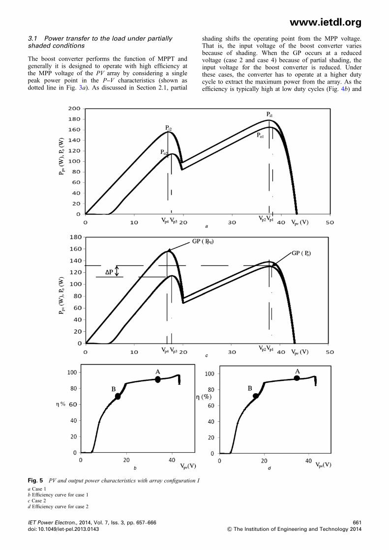
3.1 Power transfer to the load under partiallyshaded conditions
The boost converter performs the function of MPPT andgenerally it is designed to operate with high efficiency atthe MPP voltage of the PV array by considering a singlepeak power point in the P–V characteristics (shown asdotted line in Fig. 3a). As discussed in Section 2.1, partial

Fig. 5 PV and output power characteristics with array configuration I

a Case 1b Efficiency curve for case 1c Case 2d Efficiency curve for case 2


shading shifts the operating point from the MPP voltage.That is, the input voltage of the boost converter variesbecause of shading. When the GP occurs at a reducedvoltage (case 2 and case 4) because of partial shading, theinput voltage for the boost converter is reduced. Underthese cases, the converter has to operate at a higher dutycycle to extract the maximum power from the array. As theefficiency is typically high at low duty cycles (Fig. 4b) and


www.ietdl.org
decreases at high duty cycles [20], the power delivered to theload under partial shading conditions needs to be investigated.The power to the load (converter output power) is
calculated as

Po = hVpvI pv (5)

The efficiency of the converter is a function of PV operatingpoint which is defined by Vmpp and Impp which in turn arefunctions of solar irradiance, temperature and the shadingpattern. The power delivered to the load is determined forthe four shading patterns reported in Section 2.1.A boost converter with the following specifications is

taken up for study. L = 10 mH, RL = 0.4 Ω, VD = 1.8 V,RD = 0.24 Ω, Vsw = 1 V and RON = 0.2 Ω. It is ensured thatefficiency of the converter is 95% at the MPP voltage ofthe array. For the P–V characteristics shown in Fig. 3, theduty cycle is calculated by solving (2) for various operatingpoints and the power delivered to the load in each case isdetermined.

3.1.1 Case 1: group 1 receives 700 W/m2 and group 2receives 350 W/m2: The P–V characteristics for this caseshown in Fig. 3a have two peaks Pi1 and Pi2. This output ofPV array is fed as input to the boost converter and the powerdelivered to the load at each operating point is calculatedusing (5). Fig. 5a shows the input and the correspondingoutput power characteristics. It is observed that two peaksPo1 (170.2 W) and Po2 (112 W) exist on the output powercurve at 37.64 and 17.5 V, respectively. The efficiency ofthe converter at each operating point is calculated using (4)and is plotted in Fig. 5b. The efficiencies corresponding tothe peaks Pi1 and Pi2 are 95.8% (point A) and 72% (pointB), respectively. This shows the dependence of efficiencyof the converter on the output voltage (Vpv) of the PV array(i.e. input voltage of the converter).An important observation from Fig. 5a is that the peak Pi1

of PV curve (converter input power curve) occurs at Vp2,whereas peak Po1 of converter output power curve occurs atVp1. Similarly, Pi2 occurs at Vp4, whereas Po2 occurs at Vp3.This difference in voltage between the peaks indicates thatthe peak point in converter output curve is displaced fromthe peak of converter input power curve. In other words,the MPP of load is different from the MPP of the array.The above observation is verified analytically as given below.The converter output power can be written as

Po = Ppv − PLS (6)

where PLS corresponds to losses.

Table 2 Comparative study of power delivered to the load

Case PV power, W Output po

Pi1 Pi2 Pi3 Pi4 Po1 Po2

1 (Fig. 3a) 177.9 155.6 — — 170.2 1122 (Fig. 3b) 138.27 155.8 — — 133.68 112.2

3 (Fig. 3c) 157.69 139.1 104.2 66.67 147.4 126.74 (Fig. 3d ) 125.57 117.8 135.7 66.7 117.9 108.2


Differentiating (6) w.r.t to Vpv

dPo

dVpv= dPpv

dVpv− dPLS

dVpv(7)

At maximum power point of PV, dPpv/dVpv = 0Therefore

dPo

dVpv= 0− dPLS

dVpv= 0 (8)

The above equation clearly states that at MPP voltage of PVarray, the derivative of the output power with respect to PVvoltage is not equal to zero. Therefore it is evident thatmaximum power point of Po is displaced from maximumpower point of Ppv. Hence tracking of GP in converter inputpower curve does not guarantee delivering of maximumpower to the load. When GP of converter input power curveis tracked, the power delivered to the load is 170.2 W,whereas when GP of converter output power curve istracked, the power delivered to the load is 170.5 W. The gainincurred in this case is negligible as the GP of both PV andoutput power curves occur near the MPP voltage of the array.

3.1.2 Case 2: group 1 receives 700 W/m2 and group 2receives 220 W/m2: The significance of considering theP–V characteristics shown in Fig. 3b is to study the effectof the shift in the operating point from the MPP voltage ofthe array. Similar to the P–V characteristics, two peaks Po1

(133.68 W) and Po2 (112.2 W) exists on the output powercharacteristics at 37.88 and 17.78 V, respectively. However,a major difference that can be noted from Fig. 5c is that theGP (Pi2) of PV curve occurs at 17.01 V, whereas the GP(Po1) of output power curve occurs at 37.88 V. Since theefficiency of the converter at this operating voltage (pointB) is only 72%, the power delivered to the load is 112.2 W.When the GP (Po1) of output power curve is tracked, the

power delivered to the load is 133.74 W. Fig. 5c shows thegain (ΔP) incurred by tracking the output curve. Table 2provides the comparative study of the power delivered tothe load in the conventional method of tracking PV curveand proposed method. As seen from Table 2 for case 2, thepower delivered to the load is increased by 16.09% bytracking the output power curve.

3.1.3 Case 3: 1000, 850, 550 and 450 W/m2: Theperformance of the system is studied for array configurationII shown in Fig. 2b. Similar to the PV characteristics shownin Fig. 2c, the output power characteristics (Fig. 6a) hasfour peaks Po1 (147.4 W), Po2 (126.7 W), Po3 (90.19 W)and Po4 (43.4 W). The output power characteristics has four

wer, W Power delivered to load, W Gain, W

Po3 Po4 Conventionalmethod

Proposedmethod

— — 170.2 170.5 0.3 (0.18%)— — 112.2 133.71 21.51

(16.1%)90.19 43.4 147.4 147.43 0.03 (0.02%)

112.8 41.78 112.6 117.9 5.3 (4.49%)


Fig. 6 Converter input and output P–V characteristics

a Case 3b Efficiency curve for case 3c Case 4d Efficiency curve for case 4

www.ietdl.org

peaks Po1 (147.4 W), Po2 (126.7 W), Po3 (90.19 W) and Po4

(43.4 W) as shown in Fig. 6a. The efficiency of theconverter (Fig. 6b when it is operated at points A, B, C andD are 93.6, 90.6, 84.5 and 63%, respectively. The GP (Pi1)

Fig. 7 Configuration of the PV system considered for study


in P–V curve occurs at 76.4 V, whereas the GP (Po1) ofoutput power curve occurs at 76.6 V. Table 2 shows thatwhen Pi1 is tracked the power delivered to the load is147.4 W, whereas it is 147.43 W in proposed method.


Fig. 8 Experimental waveforms

a Vpv, Ipv, Vo and Io curves by varying the duty cycle – case 1b The corresponding PV power and power at the load side – case 1c Vpv, Ipv, Vo and Io curves by varying the duty cycle – case 2d The corresponding PV power and power at the load side – case 2e Vpv, Ipv, Vo and Io curves by varying the duty cycle – case 3f The corresponding PV power and power at the load side – case 3. Scale: X-axis-time – 2 s/div, Y-axis – Vpv = 10 V/div, Ipv = 2 A/div, Vo = 20 V/div andIo = 10 V/div

www.ietdl.org

It can be observed that the gain is negligible when the GP ofboth P–V and output power curve occurs near the MPPvoltage of the array.

3.1.4 Case 4: 1000, 850, 400and 260 W/m2: From theP–V characteristics shown in Fig. 2d, it is clear that the


number of prominent peak increases with the decrease inthe insolation level on the shaded panels. The power at theload side has four peaks Po1 (117.9 W), Po2(108.2 W),Po3(112.8 W) and Po4 (41.78 W). It is observed fromFig. 6c that Po1 is the GP and occurs at 78.18 V, whereasGP (Pi3) of P–V occurs at 34.7 V. Hence, when input PV


www.ietdl.org
curve Pi3 is tracked, the converter efficiency is 84.5% (pointC) in efficiency curve (Fig. 6d ) and only 112.6 W of power isdelivered to the load. However, if the output power curve Po1
is tracked, the power transferred to the load is 117.9 W.Table 2 shows that the power delivered to the load isincreased by 4.49% when output power curve is tracked.Therefore irrespective of the shading pattern, array

configuration and converter efficiency, the maximumpower is delivered to the load, when the output powercurve is tracked. It is noted from Table 2 that when thelocation of GP of PV and output power curve are closeto each other (cases 1 and 3), the gain is notappreciable. However, as the array size increases, thegain increases. When the locations of GP of PV andoutput power curve are different as in cases 2 and 4, themaximum power is delivered to the load by tracking theoutput power curve.

4 Results and discussion

A PV system consisting of a PV array, a boost converter andthe load is considered for study with a view to validate theanalytical results through experiments in the laboratory.Two solar PV modules are connected in series and a boostconverter is used as the MPPT which interfaces the PVarray with the resistive load. Although only two modulesare connected in series, it can be considered as two groupsof modules in series. The specifications of the modules areshown in Table 1 and the parameters of the boost converterare described in Section 2.2. The load resistance is keptconstant at 200 Ω. The converter input and output voltagesand currents are sensed using Hall effect voltagetransducers LV25 P and current transducers LA55P,respectively. The control algorithm is implemented inALTERA Cyclone II FPGA board and the configuration ofthe system set up is shown in Fig. 7. Three different casesare taken up for study and in each case the input PV powerand the power transferred to the load are examined.

4.1 Case 1

In the PV array, one module receives an insolation of 540W/m2, whereas the other module is artificially shaded witha transparent sheet such that it receives 310 W/m2 ofinsolation. The duty cycle is varied in steps and thevariation in converter input voltage Vpv, input current Ipv,converter output voltage Vo and the output current Io areobserved (Fig. 8a). The corresponding power curves areplotted in Fig. 8b. It is observed that two peaks exist in thePV curve with Pi1 as GP (32 W) and Pi2 as LP (25.6 W).Similarly, two peaks Po1 (27.2 W) and Po2 (16.4 W) existin the load side power curve Po. When the PV is operatedat a point corresponding to Pi1, the power transferred to theload is 27 W. However, when Po1 is tracked, the powerdelivered to the load is 27.2 W, which is 0.73% higher than

Table 3 Comparison of proposed and conventional method

Case G1, W/m2 G2, W/m2 Converter inputpower

Pi1, W Pi2, W

1 (Fig. 8b) 540 310 32 25.62 (Fig. 8d ) 560 180 17.5 253 (Fig. 8f ) 220 480 22.8 24


the power transferred to the load by tracking the GP in theconverter input power characteristics as shown in Table 3.In this case, the gain (0.2 W) is negligible.

4.2 Case 2

In this case, the difference in insolation between the modulesis increased such that one module receives 560 W/m2,whereas the other receives 180 W/m2. Fig. 8c shows theexperimental waveforms of the Vpv, Ipv, Vo and Io when theduty cycle is varied in steps and the corresponding powercurves are plotted in Fig. 8d. It is observed from Fig. 8dthat the GP (Pi2) shifts from the MPP value and occurs at areduced voltage. When this GP on input powercharacteristics is tracked, the power delivered to the load isonly 15.7 W. This is because of the inability of theconverter to operate at the same efficiency at all theoperating points.

4.3 Case 3

The significance of tracking the output power curve isrevealed through case 3. One of the modules in the string isshaded to receive 220 W/m2, whereas the other receives480 W/m2. Fig. 8e shows the experimental waveforms ofthe Vpv, Ipv, Vo and Io obtained by varying the duty cycleand the corresponding power curves are shown in Fig. 8f.As it is observed from Fig. 8f, this shading pattern leads totwo peaks in the P–V characteristics with the Pi2 as GP (24W) and Pi1 as LP (22.8 W). When GP in the P–Vcharacteristics is tracked, the power delivered to the load is15.2 W with an efficiency of 63.2%. Interestingly, it isobserved (from Table 3) that tracking the LP with theavailable power of 22.8 W, the power delivered to the loadis 18.8 W which is 19.15% higher than the powertransferred to the load by tracking the GP in the P–Vcharacteristics. It is evident that the efficiency of theconverter and the shading pattern determines the powerdelivered to the load. Therefore it is concluded that underall the cases the power delivered to the load is maximumwhen GP in the output power curve is tracked.

5 Conclusions

This paper addresses the impact of partial shading on thepower delivered to the load. The power transferred to theload under different shading patterns is analysed and it isobserved that the MPP of the load when the converterefficiency is considered is different from the MPP of the PVarray. Therefore tracking of converter input power curvedoes not guarantee maximum power transfer to the loadunder partial shading conditions. Hence, the study proposesto track the converter output power for maximum powertransferred to the load under partial shading conditions.Simulation and experimental results are presented to

Power delivered to load, W Gain, W

Conventional method Proposed method

27 (Pi1 is tracked) 27.2 (Po1 is tracked) 0.2 (0.73%)15.7 (Pi2 is tracked) 16 (Po2 is tracked) 0.3 (1.87%)15.2 (Pi2 is tracked) 18.8 (Po1 is tracked) 3.6 (19.15%)


www.ietdl.org
demonstrate that maximum power is transferred to the load bytracking the GP in the output power curve.
6 Acknowledgment

The authors would like to thank the National Mission onPower Electronics Technology (NaMPET)-Phase II, aninitiative of Department of Information Technology,Government of India for their financial support towards thiswork.

7 References

1 Bidram, A., Davoudi, A., Balog, S.: ‘Control and circuit techniques tomitigate partial shading effects in Photovoltaic arrays’, IEEEJ. Photovolt., 2012, 2, (4), pp. 532–546

2 Mutoh, N., Ohno, M., Takayoshi, I.: ‘A method for MPPT control whilesearching for parameters corresponding to weather conditions for PVgeneration systems’, IEEE Trans. Ind. Electron., 2008, 53, (4),pp. 1055–1065

3 Masoum, A.S., Mousavi Badejani, S.M., Fuchs, E.F.:‘Microprocessor-controlled new class of optimal battery chargers forphotovoltaic applications’, IEEE Trans. Energy Convers., 2004, 19,(3), pp. 599–606

4 Gules, R., De Pellegrin Pacheco, J., Hey, H.L.: ‘A maximum powerpoint tracking system with parallel connection for PV stand-aloneapplications’, IEEE Trans. Ind. Electron., 2008, 55, (7), pp. 2674–2683

5 Walker, G.R., Sernia, C.: ‘Cascaded DC–DC converter connection ofphotovoltaic modules’, IEEE Trans. Power. Electron., 2004, 19, (4),pp. 1130–1139

6 Esram, T., Chapman, L.: ‘Comparison of photovoltaic array maximumpower point tracking techniques’, IEEE Trans. Energy Convers, 2007,22, (2), pp. 439–449

7 Sera, D., Teodorescu, R., Hantschel, J., Knoll, M.: ‘Optimizedmaximum power point tracker for fast changing environmentalconditions’, IEEE Trans. Ind. Electron., 2008, 55, (7), pp. 2629–2637

8 Gomes, M.A., Galotto Jr., L., Sampaio, L., Melo, A., Canesin, C.A.:‘Evaluation of the main MPPT techniques for photovoltaicapplications’, IEEE Trans. Ind. Electron, 2013, 60, (3), pp. 1156–1167

9 Petrone, G., Spagnuolo, G., Vitelli, M.: ‘A multivariable perturb andobserve maximum power point tracking technique applied to a singlestage photovoltaic inverter’, IEEE Trans. Ind. Electron., 2011, 58, (1),pp. 76–84

10 Femia, N., Petrone, G., Spagnuolo, G., Vitelli, M.: ‘A technique forimproving P&O MPPT performance of double-stage grid-connectedphotovoltaic systems’, IEEE Trans. Ind. Electron., 2011, 58, (11),pp. 76–84

11 Safari, A., Mekhilef, S.: ‘Simulation and hardware implementation ofincremental conductance MPPT with direct control method using cukconverter’, IEEE Trans. Ind. Electron., 2011, 58, (4), pp. 1154–1161

12 Mei, Q., Shan, M., Liuand, L., Guerrero, J.M.: ‘A novel variable stepsize incremental resistance MPPT method for PV systems’, IEEETrans. Ind. Electron., 2011, 58, (4), pp. 2427–2434

13 Noguchi, T., Togashi, S., Nakamoto, R.: ‘Short-current pulse-basedmaximum-power-point tracking method for multiplephotovoltaic-and-converter module system’, IEEE Trans. Ind.Electron., 2002, 49, (1), pp. 217–223

14 Masoum, M.A.S., Dehbonei, H., Fuchs, E.F.: ‘Theoretical andexperimental analyses of photovoltaic systems with voltage and


current-based maximum power-point tracking’, IEEE Trans. EnergyConvers., 2002, 17, (4), pp. 514–522

15 Patel, H., Agarwal, V.: ‘MATLAB based modeling to study the effectsof partial shading on PV array characteristics’, IEEE Trans. EnergyConvers., 2008, 23, (1), pp. 302–310

16 M̈aki, A., Valkealahti, S.: ‘Power losses in long string and parallelconnected short strings of series-connected silicon-based photovoltaicmodules due to partial shading conditions’, IEEE Trans. EnergyConvers., 2012, 27, (1), pp. 173–183

17 Wang, Y.-J., Hsu, P.-C.: ‘Analytical modelling of partial shading anddifferent orientation of photovoltaic modules’, IET Renew. PowerGener., 2010, 4, (3), pp. 272–282

18 Syafaruddin, R., Karatepe, E., Hiyama, T.: ‘Artificial neuralnetwork-polar coordinated fuzzy controller based maximum powerpoint tracking control under partially shaded conditions’, IET Renew.Power Gener., 2009, 3, (2), pp. 239–253

19 Young-Hyok, J., Doo-Yong, J., Chung-Yuen, W., Byoung-Kuk, L.,Jin-Wook, K.: ‘A real maximum power point tracking method formismatching compensation in PV array under partially shadedconditions’, IEEE Trans. Power Electron., 2011, 26, (4), pp. 1001–1009

20 Petrone, G., Spagnuolo, G., Teodorescu, R., Veerachary, M., Vitelli, M.:‘Reliability issues in photovoltaic power processing systems’, IEEETrans. Ind. Electron., 2008, 55, (7), pp. 2569–2580

21 Kobayashi, K., Takano, I., Sawada, Y.: ‘A study on a two stagemaximum power point tracking control of a photovoltaic system underpartially shaded isolation conditions’. Proc. IEEE Power EngineeringSociety General Meeting, 2003, pp. 2612–2617

22 Koutroulis, E., Blaabjerg, F.: ‘A new technique for tracking the globalmaximum power point of PV arrays operating under partial-shadingconditions’, IEEE J. Photovolt., 2012, 2, (2), pp. 184–190

23 Ishaque, K., Salam, Z., Amjad, M., Mekhilef, S.: ‘An improved particleswarm optimization (PSO)–based MPPT for PV with reducedsteady-state oscillation’, IEEE Trans. Power Electron., 2012, 27, (8),pp. 3627–3638

24 Miyatake, M., Inada, T., Hiratsuka, I., Zhao, H., Otsuka, H., Nakano,M.: ‘Control characteristics of a Fibonacci-search-based maximumpower point tracker when a photovoltaic array is partially shaded’.Proc. IEEE IPEMC, 2004, vol. 2, pp. 816–821

25 Ramaprabha, R., Mathur, B., Ravi, A., Aventhika, S.: ‘ModifiedFibonacci search based MPPT scheme for SPVA under partial shadedconditions’. Proc. Third Int. Conf. Emerging Trends EngineeringTechnology, 2010, pp. 379–384

26 Patel, H., Agarwal, V.: ‘Maximum power point tracking scheme for pvsystems operating under partially shaded conditions’, IEEE Trans Ind.Electron., 2008, 55, (4), pp. 1689–1698

27 Femia, N., Gianpaolo, L., Giovanni, P., Spagnuolo, G., Vitelli, M.:‘Distributed maximum power point tracking of photovoltaic arrays:novel approach and system analysis’, IEEE Trans. Ind. Electron.,2008, 55, (7), pp. 2610–2621

28 Nguyen, D., Lehman, B.: ‘An adaptive solar photovoltaic array usingmodel-based reconfiguration algorithm’, IEEE Trans. Ind. Electron.,2008, 55, (7), pp. 2644–2654

29 Velasco, G., Gispert, F., Pique-lopez, L., Roca: ‘Electrical PV arrayreconfiguration strategy for energy extraction improvement in gridconnected systems’, IEEE Trans. Ind. Electron., 2009, 56, (11),pp. 4319–31

30 Erickson, W., Maksimovic, D: ‘Fundamentals of Power Electronics’(Springer International Edition, 2000, 2nd edn.)

31 Kuo, Y.-C., Liang, T.-J., Chen, J.-F.: ‘Novel maximum-power-pointtracking controller for photovoltaic energy conversion system’, IEEETrans. Ind. Electron., 2001, 48, (3), pp. 594–601


06759699

Documents