08gnss student paper pejmank 25sep08

8/2/2019 08gnss Student Paper Pejmank 25sep08

http://slidepdf.com/reader/full/08gnss-student-paper-pejmank-25sep08 1/10

__________________________________________________________________________________________

ION GNSS 2008, Session C5, Savannah, GA, 16-19 September 2008 1/10

Optimum Digital Filters for GNSS Tracking

Loops

Pejman L. Kazemi

Position, Location And Navigation (PLAN) Group

Department of Geomatics Engineering

University of Calgary

BIOGRAPHY

Pejman L. Kazemi is a Ph.D. student in the Department of

Geomatics Engineering at the University of Calgary. He

received his BSc in Electrical Engineering, majoring in

telecommunications from the Iran University of Scienceand Technology in 2006. His research interests are in

GNSS software receiver design, spread spectrum

communication and digital signal processing.

ABSTRACT

In a traditional loop filter the product between loop noise

bandwidth and integration time (BLT) should remain well

below unity in order to ensure the stability of the loop.This constraint, required for having a stable loop,

significantly limits the maximum integration time and/or noise bandwidth.

The current methodology in designing digital tracking

loop filters mostly relies on transforming a continuous-time system into a discrete-time one. This transform, from

the S-domain to Z-domain, is done by means of Laplace

to Z-domain mappings, such as the bilinear transform. In

these cases, the digital loops will be equivalent to its

analog counterpart only if BLT is close to zero (Stephens& Thomas 1995, Lindsey & Chie 1981). As the product

BLT increases, the effective loop noise bandwidth and

closed loop pole locations deviate from the desired onesand eventually the loop becomes unstable.

By designing filters with the controlled-root method the

deficiencies of the continuous-update approximation inlarge BLT applications are avoided (Stephens & Thomas

1995). However, by using this method for the

conventional NCOs (denoted as rate-only feedback NCOs

in Stephens & Thomas 1995) which are mostly used in

software receivers, the BLT is still limited to less than 0.4for third order loops.

In this paper, by considering the effect of integration anddump in the linear model of the digital phase-locked loop

and considering rate-only feedback NCOs, loop filters are

designed totally in the Z-domain by utilizing a method

that minimizes the loop phase jitter. It is shown that, by

using these new filters, a significant improvement for high BLT can be achieved, allowing one to operate in

ranges where previous methods can not operate. As a

result, stable loops with higher bandwidths and/or longer integration time can be easily designed. The deficiencies

of previous methods are analyzed and the loop instability

for large BLT is shown by employing live GPS signals.

New loop filters are implemented in a GPS softwarereceiver and their performance for large BLT evaluated by

using live GPS signals for static tests and hardware

simulated signals for dynamic tests.

INTRODUCTION

Phase-locked loops are widely used in modern

communication systems. As a result of the rapid evolutionof digital microelectronics technologies the current trend

is to implement and design phase-locked loops in the

digital domain. Especially for software receivers this is an

inevitable choice. Much research has been done in thisfield and an excellent survey of theoretical and

experimental works accomplished in this area up to 1981

can be found in (Lindsey & Chie 1981). Most research

focuses on different methods for the design of the phase

detector and very little effort has been spent on the designof loop filters.

Since theoretical and practical aspects of continuous phase-locked loops and their performance in different

situations is well known, the typical methodology in

designing digital loop filters is based on thetransformation from the analog domain (Gardner 2005,

Stephens 2001, Best 1999, Lindsey & Chie 1981). This

technique is widely used for GNSS signal tracking loops

(Ward et al 2006, Stephens 2001, Tsui 2000, Spilker

1997). In these methods, filters are first designed in the S-



__________________________________________________________________________________________


domain and then, for the digital implementation, they are

transformed into the Z-domain. Examples of analog todigital transformation methods are the bilinear, boxcar,

impulse invariant transforms. The necessary condition for

these filters to resemble their analog counterparts is tohave a BLT near zero (Lindsey & Chie 1981). As this

product increases the filter zeros are displaced with

respect to the position originally designed in the analog

domain. Moreover, changes in the open loop gain can beobserved and the true noise bandwidth tends to be larger than the target one. These phenomena can make the

system unstable. Experimentally, it was proven that by

employing transformation method, the third order loopremain stable for BLT less than 0.55.

In the controlled-root method proposed by Stephens &Thomas (1995), loop filter constants are determined

specifically for each BLT value. In this way the

deficiencies for the loop design for different BLT are

avoided and the digital loop has exactly the desired

bandwidth, however the structure of the filter remains the

same as the one obtained with the transformation method.In this case the maximum achievable BLT for a stable

loop is limited to 0.4 for rate-only feedback NCOs

(Stephens & Thomas 1995). For most communicationapplications, this condition is satisfied since BLT remains

close to zero. However for some new GNSS applications,

such as weak signal tracking and for extremely highdynamic applications, larger BLT values are required.

Configurations with a 20 ms integration time and a 60 Hz

bandwidth (BLT = 1.2) or with a 500 ms integration time

and a 3 Hz bandwidth (BLT = 1.5) are impossible with

these conventional methods.

Another method which has been rarely treated in the

literature is the minimization method. This method wasfirst used by Gupta (1968) using Z-transform and

modified Z-transform for analog-digital phase-locked

loops. In this case the phase-locked loop is the same asthe continuous case except that the filter is replaced by a

discrete filter followed by a hold circuit (Gupta 1968). In

Kumar & Hurd (1986) this minimization method was

adopted for phase-locked loops with a substantial

computation delay (transport lag). Minimization

techniques for the design of digital tracking loops haveonly been marginally considered in the literature and

tracking loops have been essentially designed by means of

transformation methods.

The main focus of this paper is the design of digital

tracking loops directly in the Z-domain based on thelinear model of the DPLL. More specifically a

minimization technique is used to determine the filter

structure and coefficients. These parameters are

determined in order to minimize the variance of the phase

error. The effect of the integration time is considered inthe linear model to extend the operational range of the

filter to larger BLT values. Instantaneous update of the

loop filter (i. e., in the absence of a computational delay)is assumed. It is shown that the transfer function of the

optimum loop filter with the rate-only feedback NCO is

different from what is currently used for most GNSSreceivers. As a result, it becomes possible to go beyond

the 0.4 BLT limit. This minimization technique for filter

design has never been applied to GNSS receivers, thus it

represents the innovative contribution of this paper. Thedetailed filter design procedure for a ramp change in theinput frequency is given. This choice of frequency input

gives a steady state error equivalent to those achievable

with a third order continuous-time loop. Finally, the performance and stability of the designed loops are shown

by means of live GPS signals for both static and dynamic

situations. Tests are conducted for BLT values at whichconventional loops cannot operate at all.

LINEAR DPLL MODEL

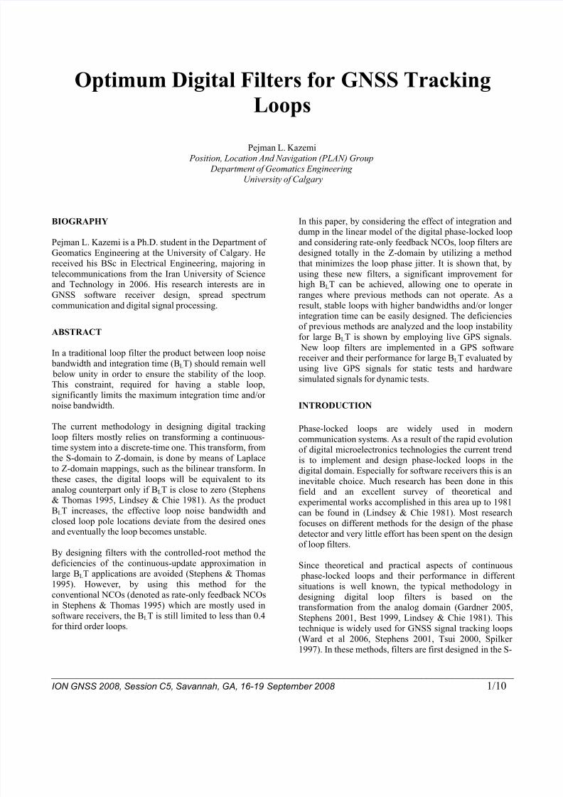
The linear model for DPLL is shown in Figure 1. The

model presented here is different form those presented inStephens (2001) and Lindsey & Chie (1981) in that the

present model explicitly accounts for the effect of the

integrate and dump blocks. Under the assumption that the phase error is small and the discriminator is operating in

its linear region, the discriminator is modeled as the

difference between the average phase of the incomingsignal and the average phase generated by the NCO in

each integration interval. F(z) represents the transfer

function of the loop filter and N(z) is the transfer function

of the NCO when the averaging effect due to the integrate

and dump block is accounted for. The input of the loop isassumed to be a phase signal affected by white Gaussian

noise with power spectral density ρ =Φiinn

. The random

component of the NCO phase, due to the input noise is

denoted by n0, and ψ represents the deterministic

component of the phase error.

in

ψ θ += on )

)( z N

-

AverageOver T

NCO

F(z)Average

Over T

θ

in

ψ θ += on )

)( z N

-

AverageOver T

NCO

F(z)Average

Over T

θ

Figure 1. Linear DPLL model.

The loop filter combines present and past values of the

residual phase, θ θ ˆ− , to obtain the estimate for the next

phase rate. In conventional NCOs (denoted as the rate-



__________________________________________________________________________________________


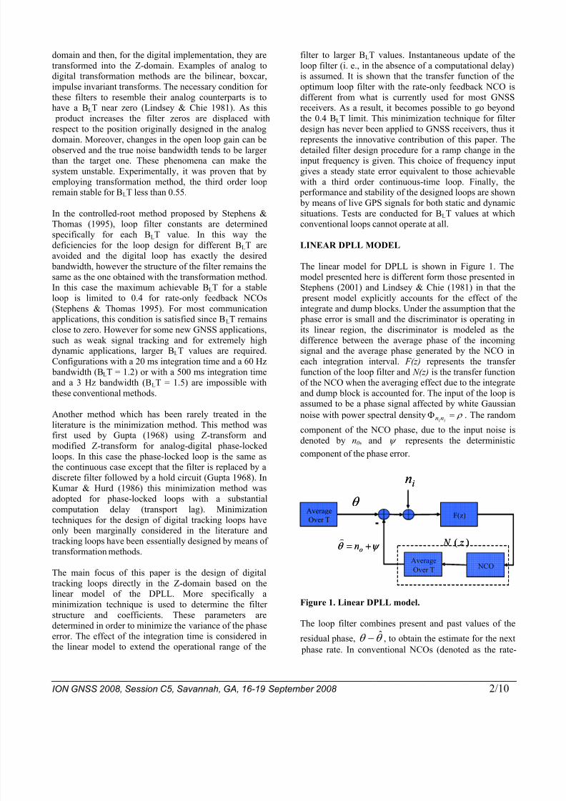
only feedback NCOs), which are the main interest of this

paper, this estimate of phase rate is used to update the NCO rate for the next integration interval. In this case,

since the phase rate is assumed to be constant over each

integration interval, the average generated phase by the NCO in each interval is equivalent to the generated phase

in the middle of the interval. As illustrated in Figure 2, the

difference equation relating the average phase on the

n+1th interval with the nth phase is given by:

)(2

11 ++ Δ+Δ+= nnnn

T ϕ ϕ ϕ ϕ (1)

where nϕ is the average generated phase, nϕ Δ is an

estimated phase rate by the loop filter and T is theintegration interval.

Nth integration interval

Time

N

C O P

h a s e

nϕ

1+nϕ

Figure 2. Schematic illustration of the NCO phase for

the rate-only feedback NCO.

Since the required parameters for generating the local

signal for the n+1 interval come from the nth

interval thereis an inherited delay in the DPLL. More specifically it is

noted that the estimated phase rate for the n+1 interval is

the loop filter output at the nth interval. By taking the Z-transform of Eq. (1) it is possible to obtain the NCO

transfer function by considering the averaging effect:

)1(2

)1()(

−

+=

z z

z T z N . (2)

From Figure 1 the close loop transfer function can be

written as:

)()(1

)()()( z N z F

z N z F z H +

= . (3)

In designing loop filters in the Z-domain, the model of the

NCO extremely impacts the transfer function of the filter

and should be accurately modeled. In the literature

different approaches have been adopted. For example, inLegrand (2001), a multi-rate model for DPLL including

the effect of integration and dump is derived. The model

will be simplified to the herein model under the valid

assumption that the predetection bandwidth is very smallas compared with the sampling frequency. In (Humphreys

et al 2005), a simple approximation is used to take into

account the effect of the integration and dump unit.Interestingly, multiplication of the Integration unit

transfer function by the NCO transfer function is also

equivalent to the model here.

Usually the NCO is modeled as1−

T (Lindsey & Chie

1981) which is not a valid model for large BLT values and

the effect of averaging should be taken into account for performance analysis in these regions.

DESIGN OF THE OPTIMUM DISCRETE FILTER

The design of the optimum digital filter is based on the

minimization of the function (Gupta 1968):

∑+=

k

k k nQ )()(22

0

ε λ (4)

where )()()( k k k ψ θ ε −= is the deterministic component

of the phase difference between incoming and generated

phase. The parameter λ is determined on the basis of noise

bandwidth considerations. The first term on the right handside of the (4) can be expressed in terms of the closed

loop transfer function H(z) as follows:

∫ ΓΦ= z

dz z

jk n nn )(

2

1)(

00

20

π (5)

where00nnΦ is the noise spectral density of 0n and is

related to the input noise spectral density by

)()()()(1

00 z z H z H z

ii nnnn Φ=Φ −. (6)

Denoting the Z transforms of )(k ε and )(k θ by E(z) and

)( z Θ , respectively, the second term of (4) can be written

as

∫

∑ ∫

Γ

−

Γ

−

Φ−−=

=

z

dz z H z H

j

z

dz z E z E

jk

k

θθ π

π ε

))(1))((1(2

1

)()(2

1)(

1

12

(7)

where:

)()( 1−ΘΘ=Φ z z θθ . (8)

From Eqs. (5) and (7) the cost function can be written as



__________________________________________________________________________________________


dz z W z W z P

z N z W z N z W j

Q

)]()()(

))()()()(1([2

1

1

11

−

−−

Γ

+

Φ−−= ∫ θθ λ π

(9)

where

)(

)()(

z N

z H z W = (10)

and

)()()]([)( 1−Φ+= z N z N z z P θθ λ ρ . (11)

By applying the standard minimization procedure to Q the

optimum solution for W(z) and thus F(z) can be found as

(Gupta 1968, Jury 1964)

)(

])(

)()([

)(

1

0 z P

z zP z z N z

z W +

+−

−

Φ

=

θθ λ

(12)

where

)()()( z P z P z P −+= . (13)

In the above )( z P + is the part of )( z P whose poles and

zeros lay inside the unit circle and +][ represents the part

of the partial fraction expansion of its argument whose

poles are inside the unit circle.

Finally from Eqs. (3), (10) and (12) the optimum digitalfilter transfer function is found as

)()(1

)()(

0

0

z N z W

z W z F

−= . (14)

The optimum filter in (14) is a function of λ and, as

mentioned earlier, this parameter is determined from

noise bandwidth considerations. More specifically thenormalized loop noise bandwidth is defined as

∫ Γ−=

z

dz z H z H

j B )()(

2

12

1

π (15)

where B is the one sided normalized loop noise

bandwidth and is related to one sided loop noise

bandwidth as

T

B B L = . (16)

The integral in (15) can be computed by expressing B interms of the coefficients of H(z). Eq. (16) shows that the

noise bandwidth is a function of the normalized noise

bandwidth and of the integration time (loop updateinterval). For instance a loop designed with a normalized

noise bandwidth of 0.5 will result in a loop noise bandwidth of 25 Hz for T=20 ms.

LOOP FILTER DESIGN FOR A FREQUENCY

RAMP INPUT

In this section the designing procedure for a filter with afrequency ramp as input is detailed. In this case the

designed loop will be equivalent to a 3rd order continuous-

time loop.

In this case, )()( 2t ut t =θ and Eq. (8) becomes

31

112

3

2

)1(

)1(

)1(

)1(

−

+⋅

−

+=Φ

−

−−

z

z z T

z

z z T θθ . (17)

The transfer function of the NCO with the averaging

effect is given by (2) and from (11), P(z) can be written as

; )1(

)1(4

))1(

14)4()44()106(

1)-(z

)44()4(4z-(

4)(

41

1234

4

234

8

234

8

5678

2

⎭⎬⎫

⎩⎨⎧

−

++++

⋅⎭⎬⎫

⎩⎨⎧

−

++++=

−

−++−+−++

++−++−++

⋅=

−

−−−−

z

edz cz bz az

z

edz cz bz az T

z

z z h z h z h

z h z h z

T z P

ρ

ρ

(18)

where

ρ

λ 4T h = . (19)

The terms in the brackets of Eq. (18) represent+

)( z P and

)( z P −

, respectively. By equating the coefficients of

equal powers of z in Eq. (18), the following set of equations are obtained:



__________________________________________________________________________________________


⎪⎪⎪

⎩

⎪⎪⎪

⎨

⎧

+=++++

−=+++

−=++

=+

−=

hed cba

habbcdced

hacbd ce

ad be

ae

610

44

4

4

1

22222

. (20)

The argument of the +][ operator in Eq. (12) can bewritten as:

3432

2351

)1)((2

)1(

)(

)()(

−++++

+=

Φ−

−

z ez dz cz bz a

z z T

z zP

z z N λ λ θθ (21)

By considering the fact that the roots of 432 ez dz cz bz a ++++ are outside the unit circle and

writing the partial fraction expansion of Eq. (21), )(0 z W

can be computed and, consequently, from Eq. (14), )( z F

is derived as:

)(

)(2

23

2

d d d d

nnn

D z C z B z AT

C z B z A z F

+++

++−= (22)

where the filter coefficients are related to coefficients in(20) and are given in the appendix. The filter structure can

be further simplified. By computing the roots of the

denominator in (22) it is found that the locations of the poles are fixed:

)1()1(

))((

2 +−

−−=

z z

z z z z z K F z z (23)

where K is the optimal gain of the filter given by

d

n

TA

A K

2−= . (24)

The zeros of Eq. (23) can be found as the roots of

nnn C z B z A ++2= 0. The structure of the proposed filter

has an extra pole and zero with respect to a conventional

third order loop filter.

In order to find the coefficients of the filter for differentnoise bandwidths, Eq. (20) should be solved for a range of

values of h. Note that, from the possible solutions of (20)

for a given h, the only acceptable one is that resulting in a

stable loop, which means that the roots of

edz cz bz az ++++ 234should lay inside the unit circle.

From these considerations the filter coefficients in Eq.

(22) or equivalently, the zeros and gain in Eq. (23) can becomputed. Finally from Eq. (3) and Eq. (15) the

normalized bandwidth is obtained.

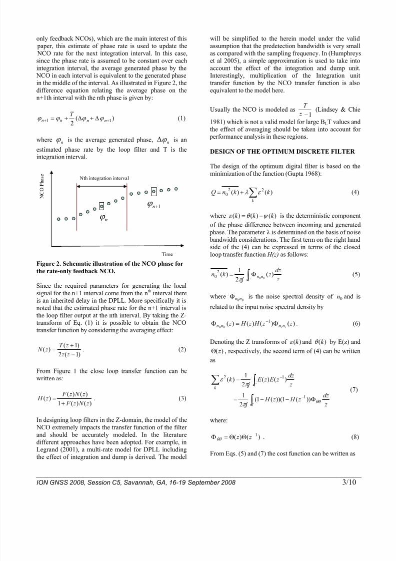
Figure 3 shows the typical value of h required to obtainthe normalized bandwidth in a large BLT region. It should

be emphasized again that all of the previous filter

structures will result in an unstable loop for a BLT larger than 0.55.

10-5

10-4

10-3

10-2

10-1

100

0

0.5

1

1.5

2

2.5

3

h Parameter

N o r m a l i z e d B a n d w i d t h ( B L

T )

Figure 3. One-sided Normalized Bandwidth versus the

h parameter.

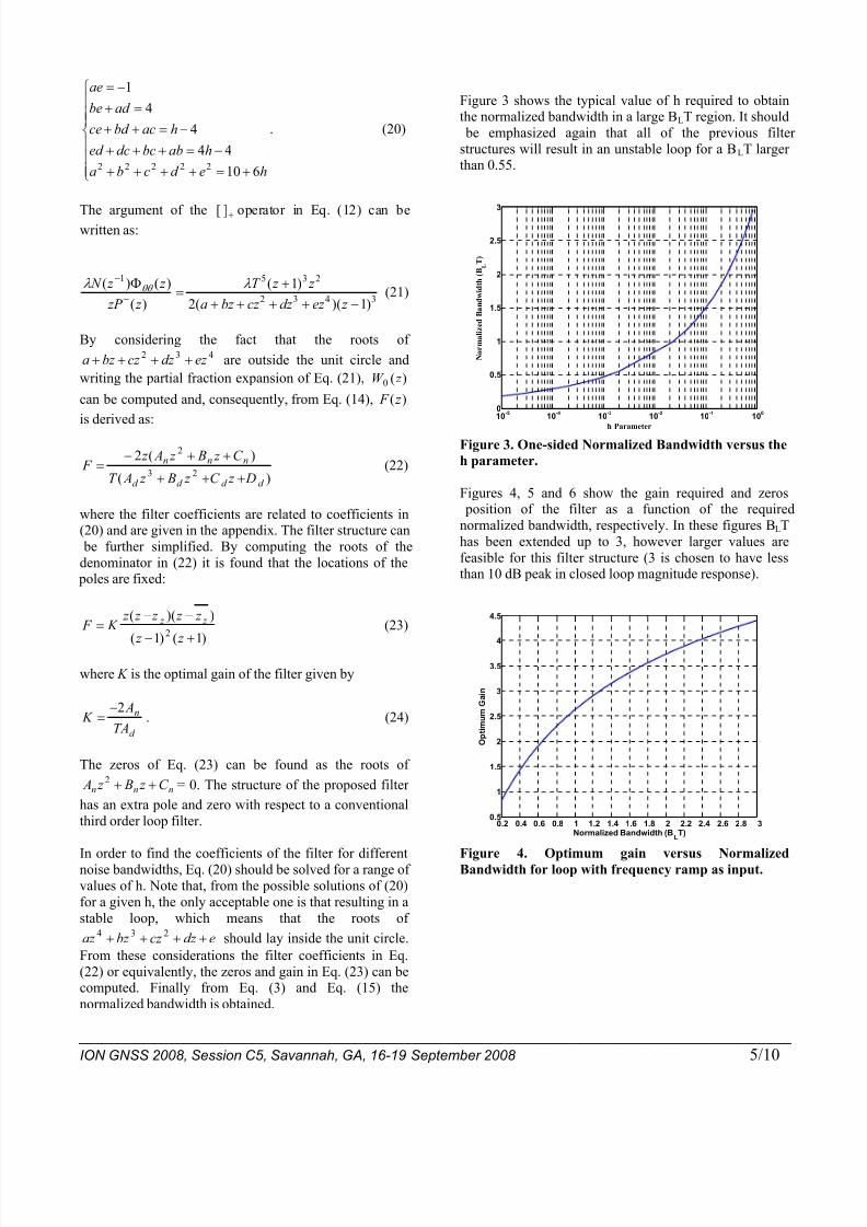
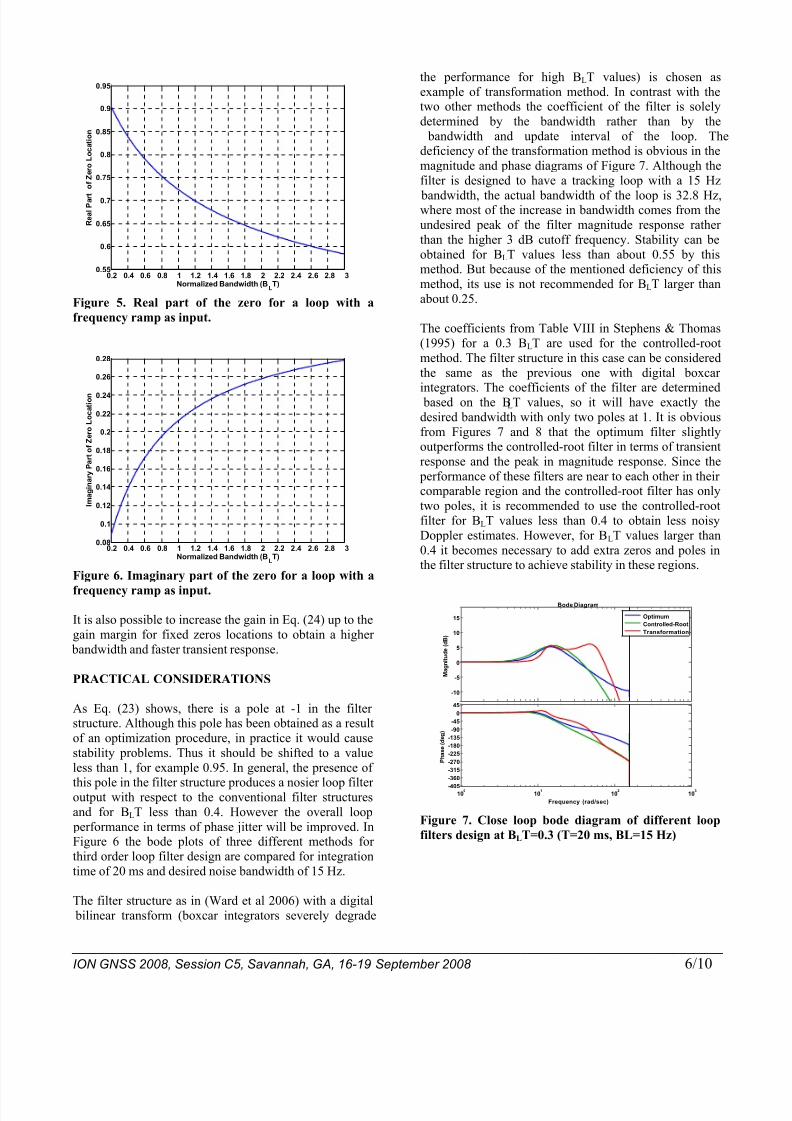
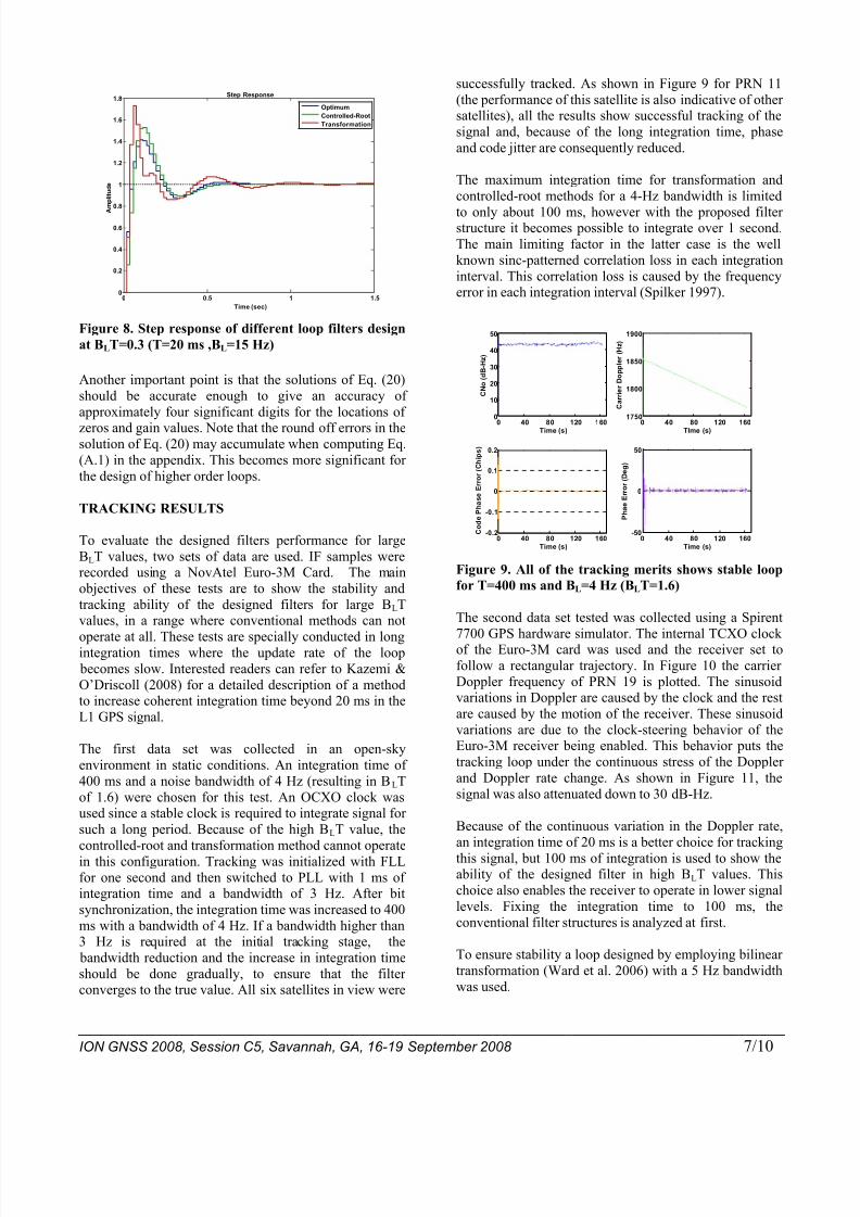
Figures 4, 5 and 6 show the gain required and zeros position of the filter as a function of the required

normalized bandwidth, respectively. In these figures BLT

has been extended up to 3, however larger values are

feasible for this filter structure (3 is chosen to have lessthan 10 dB peak in closed loop magnitude response).

0.2 0.4 0.6 0.8 1 1.2 1.4 1.6 1.8 2 2.2 2.4 2.6 2.8 30.5

1

1.5

2

2.5

3

3.5

4

4.5

Normalized Bandwidth (BLT)

O p t i m u m G a i n

Figure 4. Optimum gain versus NormalizedBandwidth for loop with frequency ramp as input.



__________________________________________________________________________________________


0.2 0.4 0.6 0.8 1 1.2 1.4 1.6 1.8 2 2.2 2.4 2.6 2.8 30.55

0.6

0.65

0.7

0.75

0.8

0.85

0.9

0.95


R e a l P a r t o f Z e r o L o c a t i o n

Figure 5. Real part of the zero for a loop with a

frequency ramp as input.

0.2 0.4 0.6 0.8 1 1.2 1.4 1.6 1.8 2 2.2 2.4 2.6 2.8 30.08

0.1

0.12

0.14

0.16

0.18

0.2

0.22

0.24

0.26

0.28


I m a g i n a r y P a r t o f Z e r o L o c a t i o n

Figure 6. Imaginary part of the zero for a loop with a

frequency ramp as input.

It is also possible to increase the gain in Eq. (24) up to the

gain margin for fixed zeros locations to obtain a higher

bandwidth and faster transient response.

PRACTICAL CONSIDERATIONS

As Eq. (23) shows, there is a pole at -1 in the filter structure. Although this pole has been obtained as a result

of an optimization procedure, in practice it would cause

stability problems. Thus it should be shifted to a value

less than 1, for example 0.95. In general, the presence of

this pole in the filter structure produces a nosier loop filter output with respect to the conventional filter structures

and for BLT less than 0.4. However the overall loop

performance in terms of phase jitter will be improved. InFigure 6 the bode plots of three different methods for

third order loop filter design are compared for integration

time of 20 ms and desired noise bandwidth of 15 Hz.

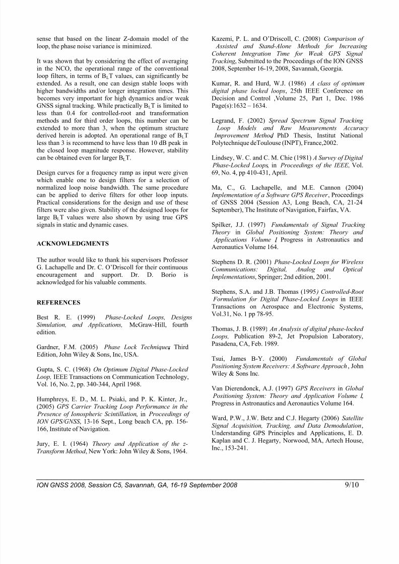
The filter structure as in (Ward et al 2006) with a digital

bilinear transform (boxcar integrators severely degrade

the performance for high BLT values) is chosen as

example of transformation method. In contrast with thetwo other methods the coefficient of the filter is solely

determined by the bandwidth rather than by the

bandwidth and update interval of the loop. Thedeficiency of the transformation method is obvious in the

magnitude and phase diagrams of Figure 7. Although the

filter is designed to have a tracking loop with a 15 Hz

bandwidth, the actual bandwidth of the loop is 32.8 Hz,where most of the increase in bandwidth comes from the

undesired peak of the filter magnitude response rather

than the higher 3 dB cutoff frequency. Stability can be

obtained for BLT values less than about 0.55 by thismethod. But because of the mentioned deficiency of this

method, its use is not recommended for BLT larger than

about 0.25.

The coefficients from Table VIII in Stephens & Thomas

(1995) for a 0.3 BLT are used for the controlled-root

method. The filter structure in this case can be considered

the same as the previous one with digital boxcar

integrators. The coefficients of the filter are determined based on the BLT values, so it will have exactly the

desired bandwidth with only two poles at 1. It is obvious

from Figures 7 and 8 that the optimum filter slightlyoutperforms the controlled-root filter in terms of transient

response and the peak in magnitude response. Since the

performance of these filters are near to each other in their comparable region and the controlled-root filter has only

two poles, it is recommended to use the controlled-root

filter for BLT values less than 0.4 to obtain less noisy

Doppler estimates. However, for BLT values larger than

0.4 it becomes necessary to add extra zeros and poles inthe filter structure to achieve stability in these regions.

-10

-5

0

5

10

15

M a g n i t u d e ( d B )

100

101

102

103

-405

-360

-315

-270

-225

-180

-135

-90

-45

0

45

P h a s e ( d e g )

Bode Diagram

Frequency (rad/sec)

Optimum

Controlled-Root

Transformation

Figure 7. Close loop bode diagram of different loop

filters design at BLT=0.3 (T=20 ms, BL=15 Hz)



__________________________________________________________________________________________


0 0.5 1 1.50

0.2

0.4

0.6

0.8

1

1.2

1.4

1.6

1.8

Step Response

Time (sec)

A m p l i t u d e

Optimum

Controlled-Root

Transformation

Figure 8. Step response of different loop filters design

at BLT=0.3 (T=20 ms ,BL=15 Hz)

Another important point is that the solutions of Eq. (20)

should be accurate enough to give an accuracy of

approximately four significant digits for the locations of

zeros and gain values. Note that the round off errors in thesolution of Eq. (20) may accumulate when computing Eq.

(A.1) in the appendix. This becomes more significant for

the design of higher order loops.

TRACKING RESULTS

To evaluate the designed filters performance for large

BLT values, two sets of data are used. IF samples wererecorded using a NovAtel Euro-3M Card. The main

objectives of these tests are to show the stability and

tracking ability of the designed filters for large BLTvalues, in a range where conventional methods can not

operate at all. These tests are specially conducted in longintegration times where the update rate of the loop

becomes slow. Interested readers can refer to Kazemi &

O’Driscoll (2008) for a detailed description of a methodto increase coherent integration time beyond 20 ms in the

L1 GPS signal.

The first data set was collected in an open-sky

environment in static conditions. An integration time of

400 ms and a noise bandwidth of 4 Hz (resulting in B LT

of 1.6) were chosen for this test. An OCXO clock wasused since a stable clock is required to integrate signal for

such a long period. Because of the high BLT value, the

controlled-root and transformation method cannot operate

in this configuration. Tracking was initialized with FLL

for one second and then switched to PLL with 1 ms of integration time and a bandwidth of 3 Hz. After bit

synchronization, the integration time was increased to 400

ms with a bandwidth of 4 Hz. If a bandwidth higher than3 Hz is required at the initial tracking stage, the

bandwidth reduction and the increase in integration time

should be done gradually, to ensure that the filter converges to the true value. All six satellites in view were

successfully tracked. As shown in Figure 9 for PRN 11

(the performance of this satellite is also indicative of other satellites), all the results show successful tracking of the

signal and, because of the long integration time, phase

and code jitter are consequently reduced.

The maximum integration time for transformation and

controlled-root methods for a 4-Hz bandwidth is limited

to only about 100 ms, however with the proposed filter structure it becomes possible to integrate over 1 second.

The main limiting factor in the latter case is the well

known sinc-patterned correlation loss in each integration

interval. This correlation loss is caused by the frequencyerror in each integration interval (Spilker 1997).

0 40 80 120 1600

10

20

30

40

50

Time (s)

C N o ( d B - H z )

0 40 80 120 160

1750

1800

1850

1900

TIme (s)

C a r r i e r D o p p l e r ( H z )

0 40 80 120 160-0.2

-0.1

0

0.1

0.2

Time (s)

C o d e P h a s e E r r o r ( C h i p s )

0 40 80 120 160

-50

0

50

Time (s)

P h a e E r r o r ( D e g )

Figure 9. All of the tracking merits shows stable loop

for T=400 ms and BL=4 Hz (BLT=1.6)

The second data set tested was collected using a Spirent

7700 GPS hardware simulator. The internal TCXO clock of the Euro-3M card was used and the receiver set to

follow a rectangular trajectory. In Figure 10 the carrier

Doppler frequency of PRN 19 is plotted. The sinusoidvariations in Doppler are caused by the clock and the rest

are caused by the motion of the receiver. These sinusoid

variations are due to the clock-steering behavior of theEuro-3M receiver being enabled. This behavior puts the

tracking loop under the continuous stress of the Doppler

and Doppler rate change. As shown in Figure 11, the

signal was also attenuated down to 30 dB-Hz.

Because of the continuous variation in the Doppler rate,

an integration time of 20 ms is a better choice for tracking

this signal, but 100 ms of integration is used to show theability of the designed filter in high BLT values. This

choice also enables the receiver to operate in lower signal

levels. Fixing the integration time to 100 ms, the

conventional filter structures is analyzed at first.

To ensure stability a loop designed by employing bilinear

transformation (Ward et al. 2006) with a 5 Hz bandwidth

was used.



__________________________________________________________________________________________


As shown in Figure 10 at around 115 seconds, because of the rapid change in the carrier Doppler frequency, the

loop was unable to track this rapid change (where the line

of sight acceleration reaches to about 0.8 G) andeventually total loss of lock occurred. Figure 11 shows

that the loss of carrier lock is followed by a loss of code

lock. As a result, a wider bandwidth is required to track

this signal successfully. However, by increasing the bandwidth from 5 Hz to 7 Hz (BLT=0.7), an instable loop

is obtained. However, the optimum filter designed from

Eq. (23) for a loop with 12 Hz bandwidth (BLT=1.2)

results in a stable loop that successfully tracks the signal.This is a significant improvement with respect to

conventional loops.

0 20 40 60 80 100 120 140 160 180-1450

-1440

-1430

-1420

-1410

-1400

-1390

-1380

-1370

-1360

Time (s)

C a r r i e r D o p p l e r ( H

z )

T=100 ms, BL=12 Hz

T=100 ms, BL=5 Hz, Trans.


Figure 10. Comparison of optimum filter carrier

Doppler estimate with conventional design.

0 20 40 60 80 100 120 140 160 180

-10

0

10

20

30

40

50

Time

C N o ( d B - H z )

T=100 ms, BL=12 Hz



Figure 11. CN0 estimate.

In DPLLs, with each update interval, the fixed locally

generated carrier frequency is correlated with the

incoming signal. The assumption of having a constantfrequency over each 100 ms is not valid in this test. The

performance is compared with an integration time of 20

ms and a bandwidth of 10 Hz. As shown in Figure 12,

changes in Doppler frequency in each 100 ms cause phase

a mismatch between the incoming and locally generatedsignals, which is correctly detected by the phase

discriminator. Epochs of the maximum mismatch exactly

correspond to the epochs with the maximum Doppler ratechange. Reducing the update interval to 20 ms could

reduce this phase mismatch, however choosing longer

update intervals becomes inevitable in very weak signal

conditions. Figure 12 shows the output of the phasediscriminator at the transition time from strong signal

power to 30 dB-Hz. It is obvious that the phase error with

100 ms remains approximately at the same level as before

(again mainly caused by the dynamics), but the phaseerror with 20 ms integration time becomes much noisier.

26 28 30 32 34-40

-30

-20

-10

0

10

20

30

40

50

Time (s)

P h a s e E r r o r ( D e g )

T=100 ms, BL=12 Hz

T=20 ms, BL=10 Hz

Figure 12. Output of the PLL discriminator.

0 20 40 60 80 100 120 140 160 180-0.25

-0.2

-0.15

-0.1

-0.05

0

0.05

0.1

0.15

0.2

Time (s)

C o d e P h a s e E r r o r ( c h i p s )

T=20 ms

T=100 ms

Figure 13. Output of the DLL discriminator.

As shown in Figure 13, the advantage of choosing 100 ms

becomes apparent in reducing code jitter since the codedoes not experience this amount of dynamics especially in

aided-DLL scheme.

CONCLUSIONS

This paper presented new filter structures for DPLLs with

rate-only feedback NCOs. Filters are optimum in the



__________________________________________________________________________________________


sense that based on the linear Z-domain model of the

loop, the phase noise variance is minimized.

It was shown that by considering the effect of averaging

in the NCO, the operational range of the conventionalloop filters, in terms of BLT values, can significantly be

extended. As a result, one can design stable loops with

higher bandwidths and/or longer integration times. This

becomes very important for high dynamics and/or weak GNSS signal tracking. While practically BLT is limited to

less than 0.4 for controlled-root and transformation

methods and for third order loops, this number can be

extended to more than 3, when the optimum structurederived herein is adopted. An operational range of BLT

less than 3 is recommend to have less than 10 dB peak in

the closed loop magnitude response. However, stabilitycan be obtained even for larger BLT.

Design curves for a frequency ramp as input were given

which enable one to design filters for a selection of

normalized loop noise bandwidth. The same procedure

can be applied to derive filters for other loop inputs.Practical considerations for the design and use of these

filters were also given. Stability of the designed loops for

large BLT values were also shown by using true GPSsignals in static and dynamic cases.

ACKNOWLEDGMENTS

The author would like to thank his supervisors Professor

G. Lachapelle and Dr. C. O’Driscoll for their continuous

encouragement and support. Dr. D. Borio is

acknowledged for his valuable comments.

REFERENCES

Best R. E. (1999) Phase-Locked Loops, Designs

Simulation, and Applications, McGraw-Hill, fourthedition.

Gardner, F.M. (2005) Phase Lock Techniques, ThirdEdition, John Wiley & Sons, Inc, USA.

Gupta, S. C. (1968) On Optimum Digital Phase-Locked Loop, IEEE Transactions on Communication Technology,Vol. 16, No. 2, pp. 340-344, April 1968.

Humphreys, E. D., M. L. Psiaki, and P. K. Kinter, Jr.,

(2005) GPS Carrier Tracking Loop Performance in the

Presence of Ionospheric Scintillation, in Proceedings of

ION GPS/GNSS , 13-16 Sept., Long beach CA, pp. 156-

166, Institute of Navigation.

Jury, E. I. (1964) Theory and Application of the z-

Transform Method , New York: John Wiley & Sons, 1964.

Kazemi, P. L. and O’Driscoll, C. (2008) Comparison of

Assisted and Stand-Alone Methods for Increasing

Coherent Integration Time for Weak GPS Signal

Tracking , Submitted to the Proceedings of the ION GNSS

2008, September 16-19, 2008, Savannah, Georgia.

Kumar, R. and Hurd, W.J. (1986) A class of optimum

digital phase locked loops, 25th IEEE Conference on

Decision and Control ,Volume 25, Part 1, Dec. 1986Page(s):1632 – 1634.

Legrand, F. (2002) Spread Spectrum Signal Tracking

Loop Models and Raw Measurements Accuracy

Improvement Method , PhD Thesis, Institut National

Polytechnique deToulouse (INPT), France,2002.

Lindsey, W. C. and C. M. Chie (1981) A Survey of Digital

Phase-Locked Loops, in Proceedings of the IEEE, Vol.

69, No. 4, pp 410-431, April.

Ma, C., G. Lachapelle, and M.E. Cannon (2004)

Implementation of a Software GPS Receiver , Proceedingsof GNSS 2004 (Session A3, Long Beach, CA, 21-24

September), The Institute of Navigation, Fairfax, VA.

Spilker, J.J. (1997) Fundamentals of Signal Tracking

Theory in Global Positioning System: Theory and

Applications Volume I , Progress in Astronautics andAeronautics Volume 164.

Stephens D. R. (2001) Phase-Locked Loops for WirelessCommunications: Digital, Analog and Optical

Implementations, Springer; 2nd edition, 2001.

Stephens, S.A. and J.B. Thomas (1995 ) Controlled-Root Formulation for Digital Phase-Locked Loops in IEEETransactions on Aerospace and Electronic Systems,

Vol.31, No. 1 pp 78-95.

Thomas, J. B. (1989) An Analysis of digital phase-locked

Loops, Publication 89-2, Jet Propulsion Laboratory,

Pasadena, CA, Feb. 1989.

Tsui, James B-Y. (2000) Fundamentals of Global

Positioning System Receivers: A Software Approach, John

Wiley & Sons Inc.

Van Dierendonck, A.J. (1997) GPS Receivers in Global

Positioning System: Theory and Application Volume I ,Progress in Astronautics and Aeronautics Volume 164.

Ward, P.W., J.W. Betz and C.J. Hegarty (2006) Satellite

Signal Acquisition, Tracking, and Data Demodulation,

Understanding GPS Principles and Applications, E. D.

Kaplan and C. J. Hegarty, Norwood, MA, Artech House,

Inc., 153-241.



__________________________________________________________________________________________


Watson, R., M.G. Petovello, G. Lachapelle and R. Klukas

(2007) Impact of Oscillator Errors on IMU-Aided GPS

Tracking Loop Performance, European Navigation

Conference, Geneva, Swizterland.

APPENDIX

In this appendix the relation between the filters

coefficients and the coefficients in Eq. (20) are given:

32be)14ce10bd

3b-9a-e-c-3d-8ab-54ae24ad(6acD

)2d2b4ac

8ad2c-4ae2e-8ab6a4ce-(4bdC)3c11ad50ae

-8ab b2ac-24ad-14bd-10ce-3e(-32beB

)8a-8ae-8ad-8ab-(-8acA

)c6ce-6ac-9e3b

24be-10bd-3d8ab46ae-24ad-9a(8deC

8ac)48ad8b

-8e-8cd96ae24ab-24a-24ce56be(24bdB

)d3c8bc19a3e

6ac24be-16ad-9b24ab10ce-42ae-(-6bdA

22222

d

22

222

d

222

22

d

2

d

222

22

n

2

22

n

2222

2

n

++

+++=

++

+++++=+++

+++=

=

++

++++=

++

++++=

++++

++++=

(A.1)

08gnss student paper pejmank 25sep08

Documents