096-31

1

Paper 096-31

Stars and Models: How to Build and Maintain Star Schemas Using SAS® Data Integration Server in SAS®9

Nancy Rausch, SAS Institute Inc., Cary, NC

ABSTRACT Star schemas are used in data warehouses as the primary storage mechanism for dimensional data that is to be queried efficiently. Star schemas are the final result of the extract, transform, and load (ETL) processes that are used in building the data warehouse. Efficiently building the star schema is important, especially as the data volumes that are required to be stored in the data warehouse increase. This paper describes how to use the SAS Data Integration Server, which is the follow-on, next generation product to the SAS ETL Server, to efficiently build and maintain star schema data structures. A number of techniques in the SAS Data Integration Server are explained. In addition, considerations for advanced data management and performance-based optimizations are discussed.

INTRODUCTION The first half of the paper presents an overview of the techniques in the SAS Data Integration Server to build and efficiently manage a data warehouse or data mart that is structured as a star schema. The paper begins with a brief explanation of the data warehouse star schema methodology, and presents the features in the SAS Data Integration Server for working with star schemas. Examples in the paper use SAS Data Integration Studio, which is the visual design component of the SAS Data Integration Server. The SAS Data Integration Server is the follow-on, next generation product to the SAS ETL Server, and SAS Data Integration Studio is the follow-on, next generation product to SAS ETL Studio. The second half of the paper provides numerous tips and techniques (including parallel processing) for improving performance, especially when working with large amounts of data. Change management and query optimization are discussed.

WHAT IS A STAR SCHEMA? A star schema is a method of organizing information in a data warehouse that enables efficient retrieval of business information. A star schema consists of a collection of tables that are logically related to each other. Using foreign key references, data is organized around a large central table, called the “fact table,” which is related to a set of typically smaller tables, called “dimension tables.” The fact table contains raw numeric items that represent relevant business facts (price, discount values, number of units that are sold, costs that are incurred, household income, and so on.). Dimension tables represent the different ways that data can be organized, such as geography, time intervals, and contact names. Data stored in a star schema is defined as being “denormalized.” Denormalized means that the data has been efficiently structured for reporting purposes. The goal of the star schema is to maintain enough information in the fact table and related dimension tables so that no more than one join level is required to answer most business-related queries.

EXAMPLE STAR SCHEMA The star schema data model used in this paper is shown in Figure 1.

Data Warehousing, Management and QualitySUGI 31

2

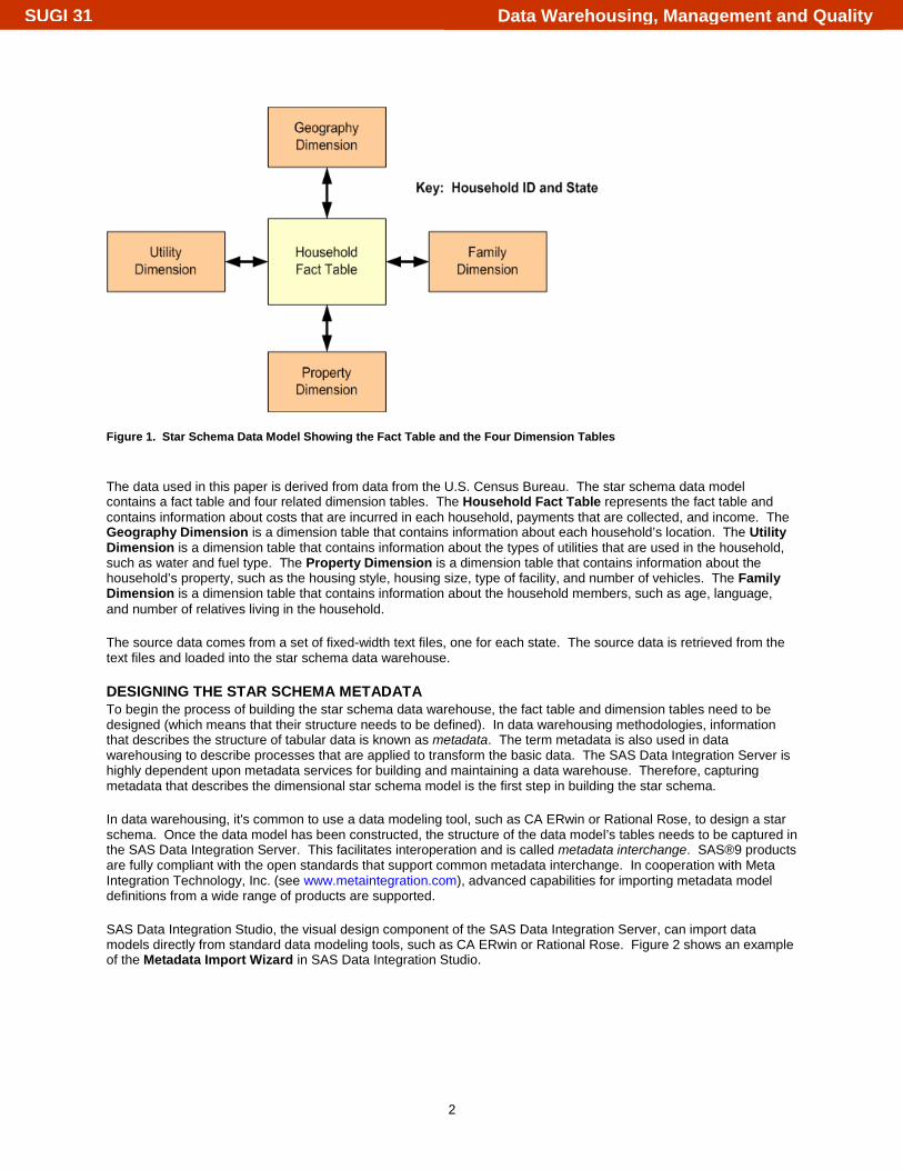
Figure 1. Star Schema Data Model Showing the Fact Table and the Four Dimension Tables The data used in this paper is derived from data from the U.S. Census Bureau. The star schema data model contains a fact table and four related dimension tables. The Household Fact Table represents the fact table and contains information about costs that are incurred in each household, payments that are collected, and income. The Geography Dimension is a dimension table that contains information about each household’s location. The Utility Dimension is a dimension table that contains information about the types of utilities that are used in the household, such as water and fuel type. The Property Dimension is a dimension table that contains information about the household’s property, such as the housing style, housing size, type of facility, and number of vehicles. The Family Dimension is a dimension table that contains information about the household members, such as age, language, and number of relatives living in the household. The source data comes from a set of fixed-width text files, one for each state. The source data is retrieved from the text files and loaded into the star schema data warehouse.

DESIGNING THE STAR SCHEMA METADATA To begin the process of building the star schema data warehouse, the fact table and dimension tables need to be designed (which means that their structure needs to be defined). In data warehousing methodologies, information that describes the structure of tabular data is known as metadata. The term metadata is also used in data warehousing to describe processes that are applied to transform the basic data. The SAS Data Integration Server is highly dependent upon metadata services for building and maintaining a data warehouse. Therefore, capturing metadata that describes the dimensional star schema model is the first step in building the star schema. In data warehousing, it's common to use a data modeling tool, such as CA ERwin or Rational Rose, to design a star schema. Once the data model has been constructed, the structure of the data model’s tables needs to be captured in the SAS Data Integration Server. This facilitates interoperation and is called metadata interchange. SAS®9 products are fully compliant with the open standards that support common metadata interchange. In cooperation with Meta Integration Technology, Inc. (see www.metaintegration.com), advanced capabilities for importing metadata model definitions from a wide range of products are supported. SAS Data Integration Studio, the visual design component of the SAS Data Integration Server, can import data models directly from standard data modeling tools, such as CA ERwin or Rational Rose. Figure 2 shows an example of the Metadata Import Wizard in SAS Data Integration Studio.


http://www.metaintegration.com

3

Figure 2. Metadata Import Wizard – Select an import format The result of the metadata import is all of the table definitions that make up the dimensional star schema. The Metadata Import Wizard transports the star schema table definitions directly from the data model design environment into the metadata. Figure 3 shows the result of the metadata that was imported from the data modelling tool. Using SAS Data Integration Studio, you can display properties of the imported tables and see their structure and/or data. The dimension tables and fact table are now ready to use when building the ETL processes to load data from the source files into the star schema tables.

Figure 3. U.S. Census Bureau Data Fact Table Structure


4

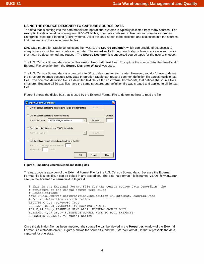
USING THE SOURCE DESIGNER TO CAPTURE SOURCE DATA The data that is coming into the data model from operational systems is typically collected from many sources. For example, the data could be coming from RDBMS tables, from data contained in files, and/or from data stored in Enterprise Resource Planning (ERP) systems. All of this data needs to be collected and coalesced into the sources that can feed into the star schema tables. SAS Data Integration Studio contains another wizard, the Source Designer, which can provide direct access to many sources to collect and coalesce the data. The wizard walks through each step of how to access a source so that it can be documented and reused. The Source Designer lists supported source types for the user to choose. The U.S. Census Bureau data source files exist in fixed-width text files. To capture the source data, the Fixed Width External File selection from the Source Designer Wizard was used. The U.S. Census Bureau data is organized into 50 text files, one for each state. However, you don't have to define the structure 50 times because SAS Data Integration Studio can reuse a common definition file across multiple text files. The common definition file is a delimited text file, called an External Format File, that defines the source file's structure. Because all 50 text files have the same structure, one definition file was created and applied to all 50 text files. Figure 4 shows the dialog box that is used by the External Format File to determine how to read the file.

Figure 4. Importing Column Definitions Dialog Box The next code is a portion of the External Format File for the U.S. Census Bureau data. Because the External Format File is a text file, it can be edited in any text editor. The External Format File is named VSAM_format1.csv, seen in the Format file name field in Figure 4.

# This is the External Format File for the census source data describing the # structure of the census source text files # Header follows Name,SASColumnType,BeginPosition,EndPosition,SASInformat,ReadFlag,Desc # Column definition records follow RECTYPE,C,1,1,,y,Record Type SERIALNO,C,2,8,,y,Serial #: Housing Unit ID PSA,C,24,26,,y,PLANNING SRVC AREA (ELDERLY SAMPLE ONLY) SUBSAMPL,C,27,28,,y,SUBSAMPLE NUMBER (USE TO PULL EXTRACTS) HOUSWGT,N,29,32,4.,y,Housing Weight ...

Once the definition file has been imported, the source file can be viewed in the Properties window of the External Format File metadata object. Figure 5 shows the source file and the External Format File that represents the data captured for one state.


5

Figure 5. Structure of a Source File after It Has Been Imported into SAS Data Integration Studio

LOADING THE DIMENSION TABLES Once the source data has been captured, the next step is to begin building the processes to load the dimension tables. You must load all of the dimension tables before you can load the fact table. The Process Designer in SAS Data Integration Studio assists in building processes to transform data. The Process Library contains a rich transformation library of pre-built processes that can be used to transform the source data into the right format to load the data model.

USING THE SCD TYPE 2 LOADER FOR SLOWLY CHANGING DIMENSIONS Although the data is not intended to change frequently in dimension tables, it will change. Households will change their addresses or phone numbers, utility costs will fluctuate, and families will grow. Changes that are made to the data stored in a dimension table are useful to track so that history about the previous state of that data record can be retained for various purposes. For example, it might be necessary to know the previous address of a customer or the previous household income. Being able to track changes that are made in a dimension table over time requires a convention to clarify which records are current and which are in the past. A common data warehousing technique used for tracking changes is called slowly changing dimensions (SCD). SCD has been discussed at length in literature, such as by Ralph Kimball (2002, 2004). The SCD technique involves saving past values in the records of a dimension. The standard approach is to add a variable to the dimension record to hold the information that indicates the status of that data record, whether it is current or in the past. The SAS Data Integration Studio SCD Type 2 Loader was designed to support this technique, has been optimized for performance, and is an efficient way to load dimension tables. The SCD Type 2 Loader supports selecting from


6

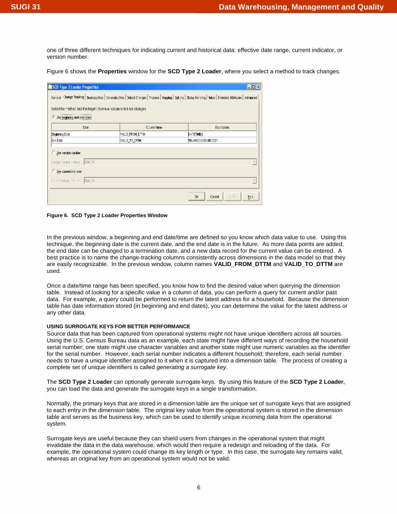
one of three different techniques for indicating current and historical data: effective date range, current indicator, or version number. Figure 6 shows the Properties window for the SCD Type 2 Loader, where you select a method to track changes.

Figure 6. SCD Type 2 Loader Properties Window In the previous window, a beginning and end date/time are defined so you know which data value to use. Using this technique, the beginning date is the current date, and the end date is in the future. As more data points are added, the end date can be changed to a termination date, and a new data record for the current value can be entered. A best practice is to name the change-tracking columns consistently across dimensions in the data model so that they are easily recognizable. In the previous window, column names VALID_FROM_DTTM and VALID_TO_DTTM are used. Once a date/time range has been specified, you know how to find the desired value when querying the dimension table. Instead of looking for a specific value in a column of data, you can perform a query for current and/or past data. For example, a query could be performed to return the latest address for a household. Because the dimension table has date information stored (in beginning and end dates), you can determine the value for the latest address or any other data.

USING SURROGATE KEYS FOR BETTER PERFORMANCE Source data that has been captured from operational systems might not have unique identifiers across all sources. Using the U.S. Census Bureau data as an example, each state might have different ways of recording the household serial number; one state might use character variables and another state might use numeric variables as the identifier for the serial number. However, each serial number indicates a different household; therefore, each serial number needs to have a unique identifier assigned to it when it is captured into a dimension table. The process of creating a complete set of unique identifiers is called generating a surrogate key. The SCD Type 2 Loader can optionally generate surrogate keys. By using this feature of the SCD Type 2 Loader, you can load the data and generate the surrogate keys in a single transformation. Normally, the primary keys that are stored in a dimension table are the unique set of surrogate keys that are assigned to each entry in the dimension table. The original key value from the operational system is stored in the dimension table and serves as the business key, which can be used to identify unique incoming data from the operational system. Surrogate keys are useful because they can shield users from changes in the operational system that might invalidate the data in the data warehouse, which would then require a redesign and reloading of the data. For example, the operational system could change its key length or type. In this case, the surrogate key remains valid, whereas an original key from an operational system would not be valid.


7

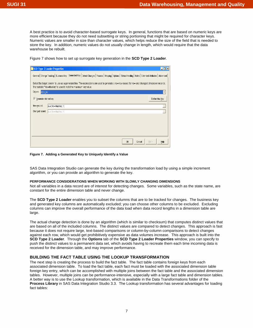
A best practice is to avoid character-based surrogate keys. In general, functions that are based on numeric keys are more efficient because they do not need subsetting or string portioning that might be required for character keys. Numeric values are smaller in size than character values, which helps reduce the size of the field that is needed to store the key. In addition, numeric values do not usually change in length, which would require that the data warehouse be rebuilt. Figure 7 shows how to set up surrogate key generation in the SCD Type 2 Loader.

Figure 7. Adding a Generated Key to Uniquely Identify a Value SAS Data Integration Studio can generate the key during the transformation load by using a simple increment algorithm, or you can provide an algorithm to generate the key.

PERFORMANCE CONSIDERATIONS WHEN WORKING WITH SLOWLY CHANGING DIMENSIONS Not all variables in a data record are of interest for detecting changes. Some variables, such as the state name, are constant for the entire dimension table and never change. The SCD Type 2 Loader enables you to subset the columns that are to be tracked for changes. The business key and generated key columns are automatically excluded; you can choose other columns to be excluded. Excluding columns can improve the overall performance of the data load when data record lengths in a dimension table are large. The actual change detection is done by an algorithm (which is similar to checksum) that computes distinct values that are based on all of the included columns. The distinct values are compared to detect changes. This approach is fast because it does not require large, text-based comparisons or column-by-column comparisons to detect changes against each row, which would get prohibitively expensive as data volumes increase. This approach is built into the SCD Type 2 Loader. Through the Options tab of the SCD Type 2 Loader Properties window, you can specify to push the distinct values to a permanent data set, which avoids having to recreate them each time incoming data is received for the dimension table, and may improve performance.

BUILDING THE FACT TABLE USING THE LOOKUP TRANSFORMATION The next step is creating the process to build the fact table. The fact table contains foreign keys from each associated dimension table. To load the fact table, each fact must be loaded with the associated dimension table foreign key entry, which can be accomplished with multiple joins between the fact table and the associated dimension tables. However, multiple joins can be performance-intensive, especially with a large fact table and dimension tables. A better way is to use the Lookup transformation, which is available in the Data Transformations folder of the Process Library in SAS Data Integration Studio 3.3. The Lookup transformation has several advantages for loading fact tables:


8

• It uses the fast-performing, DATA step hash technique as the lookup algorithm for matching source values from the fact table to the dimension tables.

• It allows multi-column key lookups and multi-column propagation into the target table. • It supports WHERE clause extracts on dimension tables for subsetting the number of data records to use in

the lookup and for subsetting the most current data records if the dimension table is using the SCD Type 2 Loader.

• It allows customizing error-handling in the data source or dimension data, such as what to do in the case of missing or invalid data values.

Figure 8 shows the process flow diagram that is used to build the fact table for the U.S. Census Bureau data.

Figure 8. The Process Flow Diagram for the U.S. Census Bureau Data The next example shows how to configure the Lookup transformation to build fact table data from associated dimension tables. The first step is to configure each lookup table in the Lookup transformation. The Source to Lookup Mapping tab is used to indicate the columns to use to match the incoming source record to the dimension table. In this case, the correct information is the surrogate key of the dimension table. In the U.S. Census Bureau data, the SERIALNO and STATE attributes represent the values that are used when matching. Because the Lookup transformation supports multi-column keys, this is easy to configure as shown in Figure 9.


9

Figure 9. Configuring the Lookup Transformation to Load the Fact Table Once the attributes to match on are defined, the next step in configuring the Lookup transformation is to identify the columns that are to be pulled out of the dimension table and propagated to the fact table. In the case of the U.S. Census Bureau data, this includes the surrogate key and any value that might be of interest to retain in the fact table. Other values worth considering are the bdate (begin date) or edate (end date) of the values that are being pulled from the dimension table. Because the Lookup transformation supports multi-column keys, any number of attributes can be pulled out of each dimension table and retained in the fact table. Using the underlying DATA step hash technique enables the Lookup transformation to scale and perform well for complex data situations, such as compound keys or multiple values that are propagated to the fact table (Figure 10).

Figure 10. Lookup Transformation Showing the Surrogate Key and End Date Propagating to the Fact Table


10

The Lookup transformation supports subsetting the lookup table via a WHERE clause. For example, you might want to perform the lookup on a subset of the data in the dimension table, so that you look up only those records that are marked as current. In that case, all other records are ignored during the lookup. In addition, the Lookup transformation supports customizing error-handling in the data source or in the dimension data. The error-handling can be customized per lookup; for example, special error-handling can be applied to the Property Dimension table that is different from what is applied to the Utility Dimension table. Customized error-handling can be useful if the data in one dimension table has a different characteristic-- for example, a lot of missing values. Multiple error-handling conditions can be specified so that multiple actions are performed when a particular error occurs. For example, an error-handling condition could specify that if a lookup value is missing, the target value should be set to “missing” and the row that contains the error should be written to an error table (Figure 11).

Figure 11. Customizable Error-Handling in the Lookup Transformation The Lookup transformation supports multiple error tables that can be generated to hold errors. An error table with a customizable format can be created to hold errors in any incoming data. An exception table with a customizable format can be created to record the conditions that generated an error (Figure 12).


11

Figure 12. Selecting Columns from the Source Data That Will Be Captured in the Error Table You can specify how to handle processes that fail. For example, a load process for a dimension table might fail, which might cause subsequent loads, such as the fact table load, to fail. If error-handling has been configured to collect errors in an error table, then the error table could get large. You can set a maximum threshold on the number of errors, so that if the threshold is reached, an action is performed, such as to abort the process or terminate the step. The error tables and exception tables are visible in the process flow diagram as registered tables (Figure 13). Separating these tables into two tables enables you to retain the format of the incoming data to fix the errors that are found in the incoming data, and then feed the data back into the process. It enables you to join the two tables into one table that describes the errors that exist in a particular record. And, it enables you to do impact analysis on both tables.

Figure 13. Optional Error Tables Are Displayed (If Selected) in the Process Flow Diagram

A MORE COMPLEX LOOKUP EXAMPLE The Lookup transformation is especially useful when the process’s complexity increases because the hash-based lookup easily handles multi-column keys and multiple lookups without sacrificing performance. For example, in the U.S. Census Bureau data, suppose that each fact table was extended so that it retained the household serial number assigned by each state, the state name, and the date the information was recorded. This information might be retained for simple historical reporting, such as growth in median household income between several census periods.


12

To add this information to the fact table, additional detail needs to be retrieved. This detail might be in the dimension tables, or it might be in a third table that is tied to the dimension table and referenced by a natural key. An example of this extended data model with the associated fields is shown in Figure 14.

Figure 14. Extended Data Model Adding the complexity to include these associated fields can degrade the performance of the process when using traditional methods, such as joins or formats. It can also increase the complexity of the code to handle the process. However, by using the Lookup transformation, the task becomes easy. An additional table can be added as another lookup entry in the Lookup transformation (Figure 15).

Figure 15. Lookup Transformation Using Multiple Tables Once the additional table has been added, the associated fields can be pulled directly from the new table (Figure 16).


13

Figure 16. The Lookup Transformation Supports Multiple Keys Pulled from the Data The code that the Lookup transformation generates is shown in the next portion of code. The composite key value is added to the hash table as another part of the lookup key, and any number of values can be pulled directly from the hash table.

/* Build hash h3 from lookup table CMAIN.Household_income */ declare hash h3(dataset:"CMAIN.Household_income"); h3.defineKey("SERIALNO", "STATE"); h3.defineData("INCOME", "YEARS"); h3.defineDone();

This example shows the simplicity and scalability of the hash-based technique in the Lookup transformation.

PERFORMANCE CONSIDERATIONS WITH LOOKUP When performing lookups, the DATA step hash technique places the dimension table into memory. When the DATA step reads the dimension table, it hashes the lookup key and creates an in-memory hash table that is accessed by the lookup key. The hash table is destroyed when the DATA step ends. Looking up a hash object is ideal for a one-time lookup step-- it builds rapidly, consumes no disk space, handles multi-column keys, and looks up fast. CPU time comparisons show that using a hash object is 33 percent to 50 percent faster than using a format. Elapsed times vary if resources are unavailable to store the hash tables in memory. Additional performance considerations when using the Lookup transformation to load the fact table are listed:

1. Make sure you have enough available RAM to hold the hash table. Adjust the MEMSIZE option to be large enough to hold the in-memory hash table and support other SAS memory needs. However, beware of increasing the MEMSIZE option far beyond the amount of available physical memory because system paging decreases job performance.

2. When running jobs in parallel, as described next, ensure that each job has enough physical RAM to hold the format or hash object because they are not shared between jobs.

3. The hash object easily supports composite keys and composite data fields.


14

The following results show the fast performance times that can be achieved using a hash object. These results were captured using a 1,000,000-row dimension table that is 512 bytes wide. Lookups from a 10,000,000-row fact table are performed against the dimension table. All fact table rows match to a dimension table row. The source code was generated using the SAS Data Integration Studio Lookup transformation.

/* Create the in-memory hash and perform the lookup. */ data lookup(keep=lookup_data lookup_key); if _N_ = 1 then do; declare hash h(dataset: "local.dimension", hashexp: 16); h.defineKey('lookup_key'); h.defineData('lookup_data'); h.defineDone(); end; set local.fact; rc = h.find(); if (rc = 0) then output; run; NOTE: The data set WORK.LOOKUP has 10000000 observations and 2 variables. NOTE: DATA statement used (Total process time): real time 30.17 seconds user cpu time 27.60 seconds system cpu time 2.52 seconds

MANAGING CHANGES AND UPDATES TO THE STAR SCHEMA Over time, the data structures used in the tables of the star schema will likely require updates. For example, the lengths of variables might need to be changed, or additional variables might need to be added or removed. Additional indexes or keys might need to be added to improve query performance. These types of updates necessitate a change to the existing data structure of the fact table and/or dimension tables in the star schema. SAS Data Integration Studio 3.3 provides useful features for understanding the impact and managing the change to the star schema tables. The features enable you to:

• Compare and contrast proposed changes to the existing and already deployed data structures. • View the impact that the changes will have on the enterprise, including the impact on tables, columns,

processes, views, information maps, and other objects in the enterprise that may be affected. • Selectively apply and merge changes to the existing data structures in a change-managed or non-change-

managed environment. • Apply changes to tables, columns, indexes, and keys.

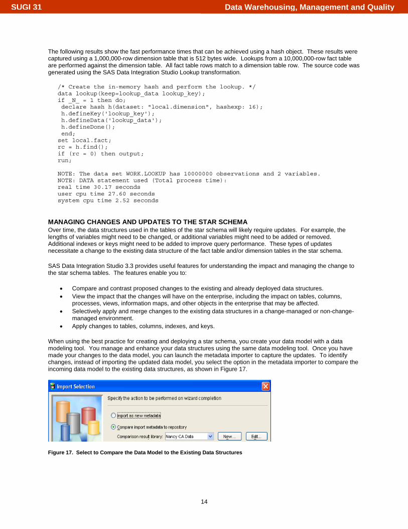
When using the best practice for creating and deploying a star schema, you create your data model with a data modeling tool. You manage and enhance your data structures using the same data modeling tool. Once you have made your changes to the data model, you can launch the metadata importer to capture the updates. To identify changes, instead of importing the updated data model, you select the option in the metadata importer to compare the incoming data model to the existing data structures, as shown in Figure 17.

Figure 17. Select to Compare the Data Model to the Existing Data Structures


15

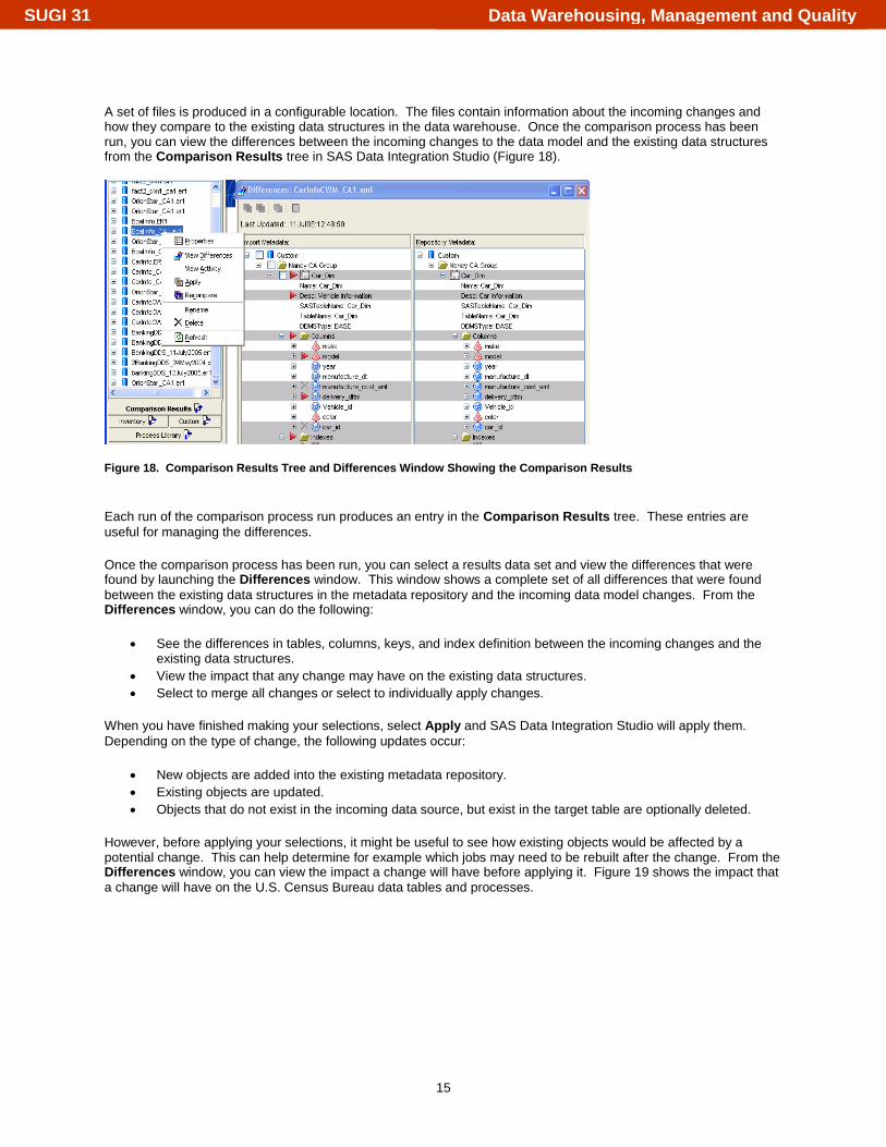
A set of files is produced in a configurable location. The files contain information about the incoming changes and how they compare to the existing data structures in the data warehouse. Once the comparison process has been run, you can view the differences between the incoming changes to the data model and the existing data structures from the Comparison Results tree in SAS Data Integration Studio (Figure 18).

Figure 18. Comparison Results Tree and Differences Window Showing the Comparison Results Each run of the comparison process run produces an entry in the Comparison Results tree. These entries are useful for managing the differences. Once the comparison process has been run, you can select a results data set and view the differences that were found by launching the Differences window. This window shows a complete set of all differences that were found between the existing data structures in the metadata repository and the incoming data model changes. From the Differences window, you can do the following:

• See the differences in tables, columns, keys, and index definition between the incoming changes and the existing data structures.

• View the impact that any change may have on the existing data structures. • Select to merge all changes or select to individually apply changes.

When you have finished making your selections, select Apply and SAS Data Integration Studio will apply them. Depending on the type of change, the following updates occur:

• New objects are added into the existing metadata repository. • Existing objects are updated. • Objects that do not exist in the incoming data source, but exist in the target table are optionally deleted.

However, before applying your selections, it might be useful to see how existing objects would be affected by a potential change. This can help determine for example which jobs may need to be rebuilt after the change. From the Differences window, you can view the impact a change will have before applying it. Figure 19 shows the impact that a change will have on the U.S. Census Bureau data tables and processes.


16

Figure 19. The Impact of a Potential Change When you work in a project repository that is under change management, the record-keeping that is involved can be useful. After you select Apply from the Differences window, SAS Data Integration Studio will check out all of the selected objects from the parent repository that need to be changed and apply the changes to the objects. Then, you can make any additional changes in the project repository. Once you have completed the changes, you check the project repository back in, which applies a change history record to all changes made in the project. Using this methodology, you retain information about the changes that are made over time to the data warehouse tables and processes.

IMPROVING PERFORMANCE WHEN WORKING WITH LARGE DATA Building efficient processes to extract data from operational systems, transform it, and then load it into the star schema data model is critical to the success of the data warehouse process. Efficiency takes on a greater importance as data volumes and complexity increase. This section describes some simple techniques that can be applied to your processes to improve their performance and efficiency. One simple technique when working with data is to minimize the number of times that the data is written to disk. Consolidate steps and use views to access the data directly. As soon as the data comes in from the operational system or files, consider dropping any columns that are not required for subsequent transformations in the flow. Make aggregations early in the flow so that extraneous detail data is not being carried between transformations in the flow. To drop columns, open the Properties window for the transformation and select the Mapping tab. Remove the extra columns from the target table area. You can turn off automatic mapping for a transformation by right-clicking the transformation in the flow, and then deselecting the Automap option in the pop-up menu. You can build your own transformation output table columns early in a flow to match as closely as possible to your ultimate target table, and map as necessary. When you perform mappings, consider the level of detail that is being retained. Ask yourself these questions.

• Is the data being processed at the right level of detail? • Can the data be aggregated in some way?


17

Aggregations and summarizations eliminate redundant information and reduce the number of records that have to be retained, processed, and loaded into the data warehouse. Ensure that the size of the variables that are being retained in the star schema are appropriate for the data length. Consider both the current use and future use of the data. Ask yourself if the columns will accommodate future growth in the data. Data volumes multiply quickly, so ensure that the variables that are being stored are the right size for the data. As data is passed from step to step in a flow, columns could be added or modified. For example, column names, lengths, or formats might be added or changed. In SAS Data Integration Studio, these modifications to a table, which are done on a transformation’s Mapping tab, often result in the generation of an intermediate SQL view step. In many situations, that intermediate SQL view step will add processing time. Avoid generating these steps. Instead of modifying and adding columns throughout many transformations in a flow, rework your flow so that you modify and add columns in fewer transformations. Avoid using unnecessary aliases; if the mapping between columns is one to one, keep the same column names. Avoid multiple mappings on the same column, such as converting a column from a numeric value to a character value in one transformation, and then converting it back in another transformation. For aggregation steps, rename columns within those transformations, rather than in subsequent transformations. Clean and deduplicate the incoming data early when building the data model tables so that extra data is eliminated quickly. This can reduce the volume of data that is sent through to the target data tables. To clean the data, consider using the Sort transformation with the NODUPKEY option, the Data Validation transformation, or use the profiling tools available in dfPower Profile. The Data Validation transformation can perform missing-value detection and invalid-value validation in a single pass of the data. It is important to eliminate extra passes over the data, so code all of these detections and validations in a single transformation. The Data Validation transformation provides deduplication capabilities and error-handling. Avoid or minimize remote data access in the context of a SAS Data Integration Studio job. When code is generated for a job, it is generated in the current context. The context includes the default SAS Application Server at the time that the code was generated for the job, the credentials of the person who generated the code, and other information. The context of a job affects the way that data is accessed when the job is executed. To minimize remote data access, you need to know the difference between local data and remote data. Local data is addressable by the SAS Application Server at the time that the code was generated for the job. Remote data is not addressable by the SAS Application Server at the time that the code was generated for the job. For example, the following data is considered local in a SAS Data Integration Studio job.

• Data that can be accessed as if it were on the same computer(s) as the SAS Workspace Server component(s) of the default SAS Application Server

• Data that is accessed with a SAS/ACCESS engine (used by the default SAS Application Server).

The following data is considered remote in a SAS Data Integration Studio job.

• Data that cannot be accessed as if it were on the same computer(s) as the SAS Workspace Server component(s) of the default SAS Application Server

• Data that exists in a different operating environment from the SAS Workspace Server component(s) of the default SAS Application Server (such as MVS data that is accessed by servers that are running under Microsoft Windows).

Remote data has to be moved because it is not addressable by the relevant components in the default SAS Application Server at the time that the code was generated. SAS Data Integration Studio uses SAS/CONNECT software and the UPLOAD and DOWNLOAD procedures to move data. It can take longer to access remote data than local data, especially for large data sets. It is important to understand where the data is located when you are using advanced techniques, such as parallel processing, because the UPLOAD and DOWNLOAD procedures run in each iteration of the parallel process.


18

In general, each step in a flow creates an output table that becomes the input of the next step in the flow. Consider what format is best for transferring this data between the steps in the flow. The choices are:

• Write the output for a step to disk (in the form of SAS data files or RDBMS tables). • Create views that process input and pass the output directly to the next step, with the intent of bypassing

some writes to disk. Some useful tips to consider are:

• If the data that is defined by a view is only referenced once in a flow, then a view is usually appropriate. If the data that is defined by a view is referenced multiple times in a flow, then putting the data into a physical table will likely improve overall performance. As a view, SAS must execute the underlying code repeatedly, each time the view is accessed.

• If the view is referenced once in a flow, but the reference is a resource-intensive procedure that performs multiple passes of the input, then consider using a physical table.

• If the view is SQL and referenced once in a flow, but the reference is another SQL view, then consider using a physical table. SAS SQL optimization can be less effective when views are nested. This is especially true if the steps involve joins or RDBMS tables.

Most of the standard transformations that are provided with SAS Data Integration Studio have a Create View option on the Options tab or a check box to configure whether the transformation creates a physical table or a view.

LOADING FACT TABLES AND DIMENSION TABLES IN PARALLEL Fact tables and dimension tables in a star schema can be loaded in parallel using the parallel code generation techniques that are available in SAS Data Integration Studio 3.3. However, the data must lend itself to a partitioning technique to be able to be loaded in parallel. Using the partitioning technique, you can greatly improve the performance of the star schema loads when working with large data. When using parallel loads, remember that the load order relationship needs to be retained between dimension tables and the fact table. All dimension table loads need to be complete prior to loading the fact table. However, if there are no relationships between the various dimension tables, which is normal in a well-designed dimensional data model, the dimension table loads can be performed in parallel. Once the dimension table loads have completed, the fact table load can begin as the last step in loading the dimensional data model. Performance can be optimized when the data that is being loaded into the star schema can be logically partitioned by some value, such as state or week. Then, multiple dimensional data models can be created and combined at a later time for the purpose of reporting, if necessary. The partitioned data can be loaded into each data model separately, in parallel; the resulting set of tables comprises the dimensional data model. In this case, two queries, at most, would be made to access the data if it is left in this form; one query would return the appropriate tables based on the logical partition, and the other query would return the fact/dimension information from the set. The output of the set of tables could be recombined by appending the resulting set of fact tables together into a larger table, or by loading the data into a database partition, such as a SAS Scalable Performance Data Server cluster partition, which retains the data separation, but allows the table to appear as a single, unified table when querying. SAS Data Integration Studio contains helpful features for parallelizing flows. These features support sequential and parallel iteration. The parallel iteration process can be run on a single multi-processor machine or on a grid system. A grid system is a web of compute resources that are logically combined into a larger shared resource. The grid system offers a resource-balancing effect by moving grid-enabled applications to computers with lower utilization, which absorbs unexpected peaks in activity. In the example used in this paper, the U.S. Census Bureau data was easily partitioned into multiple fact table and dimension table loads by partitioning the data into individual states. Benchmark performance tests were first performed using the original data, which consisted of all 50 states run together in one load. Then, after the data was partitioned, the benchmark performance tests were rerun for each state, in parallel, to create individual star schema partitions. Figure 20 shows the new flow that was run in parallel for each of the 50 states.


19

Figure 20. Parallel Processing to Run the Star Schema Load Jobs The loop transformation used in the flow enables control of the inner job, which was the original dimension table and fact table load for a single state. The loop transformation feeds substitution values into the inner job. In the U.S. Census Bureau data, each record in the table of all 50 states contains the name of the substitution values for the source state table, and the target state fact table and dimension tables. Figure 21 shows the loop transformation Properties window and some of the configuration settings that are available using the loop transformation. The loop transformation can be configured to iterate sequentially or in parallel over the inner job. The logs from each run can be collected for analysis in a user-specified location, and additional configuration settings can control how many processes should be run concurrently. The loop transformation generates SAS MP CONNECT code to manage and submit each parallel process.

Figure 21. Loop Transformation Configuration Settings The baseline performance number for processing all data sequentially in a large-scale star schema build for the U.S. Census Bureau data run across all 50 states using more than 50 gigabytes of data was 588 minutes on server class hardware. Then the same data and processes were run in parallel using the same hardware. The execution time when run in parallel was 100 minutes, representing a 5x performance improvement over the original sequential load process. The performance improvement was achieved by configuring the loop transformation settings only; no special I/O customizations were performed. However, I/O customizations could further improve the baseline performance numbers.

OPTIMIZING PERFORMANCE WHEN BUILDING SUMMARIZED DATA FROM STAR SCHEMAS Once data has been built into the star schema, the data is ready to be delivered to downstream SAS BI applications. Typically, SAS BI applications perform queries on the data. There are several techniques that SAS Data Integration


20

Studio provides to enhance performance when performing queries from a star schema. Using SAS Data Integration Studio, you can build additional summarized tables that can serve as input to other SAS BI applications. The processes that are needed to build summarized tables involve joins. SAS Data Integration Studio provides an SQL Join transformation that can be used to build summarized tables from the star schema. In this section, we describe techniques for optimizing join performance. The pains associated with joins are:

• Join performance is perceived as slow. • It’s not clear how joins, especially multi-way joins, work. • There’s an inability to influence the join algorithm that SAS SQL chooses. • There’s a higher than expected disk space consumption. • It’s hard to operate SAS SQL joins with RDBMS tables.

INITIAL CONSIDERATIONS It is common for ETL processes to perform lookups between tables. SAS Data Integration Studio provides the customizable Lookup transformation, which normally outperforms a SQL join, so consider the Lookup transformation for lookups. Joins tend to be I/O-intensive. To help minimize I/O and to improve performance, drop unneeded columns, minimize column widths (especially in RDBMS tables), and delay the inflation of column widths (this usually happens when you combine multiple columns into a single column) until the end of your flow. Consider these techniques especially when working with very large RDBMS tables.

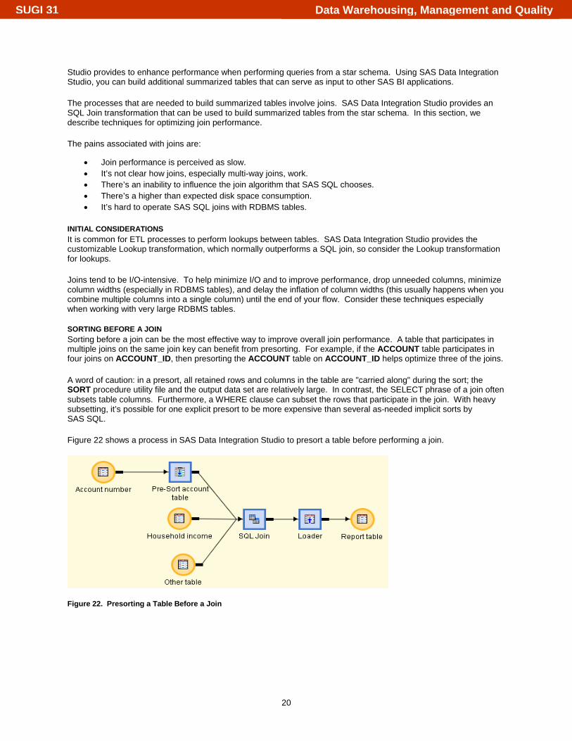
SORTING BEFORE A JOIN Sorting before a join can be the most effective way to improve overall join performance. A table that participates in multiple joins on the same join key can benefit from presorting. For example, if the ACCOUNT table participates in four joins on ACCOUNT_ID, then presorting the ACCOUNT table on ACCOUNT_ID helps optimize three of the joins. A word of caution: in a presort, all retained rows and columns in the table are "carried along" during the sort; the SORT procedure utility file and the output data set are relatively large. In contrast, the SELECT phrase of a join often subsets table columns. Furthermore, a WHERE clause can subset the rows that participate in the join. With heavy subsetting, it’s possible for one explicit presort to be more expensive than several as-needed implicit sorts by SAS SQL. Figure 22 shows a process in SAS Data Integration Studio to presort a table before performing a join.

Figure 22. Presorting a Table Before a Join


21

OPTIMIZING SELECT COLUMN ORDERING A second technique to improve join performance is to order columns in the SELECT phrase as follows:

• non-character (numeric, date, datetime) columns first • character columns last

In a join context, all non-character columns consume 8 bytes. This includes SAS short numeric columns. Ordering non-character (numeric, date, datetime) columns first perfectly aligns internal SAS SQL buffers so that the character columns, which are listed last in the SELECT phrase, are not padded. The result is minimized I/O and lower CPU consumption, particularly in the sort phase of a sort-merge join. In SAS Data Integration Studio, use a transformation’s Mapping tab to sort columns by column type, and then save the order of the columns.

DETERMINING THE JOIN ALGORITHM SAS SQL implements several well-known join algorithms-- sort-merge, index, and hash. The default technique is sort-merge. Depending on the data, index and hash joins can outperform the sort-merge join. You can influence the technique that is selected by the SAS SQL optimizer; however, if the SAS SQL optimizer cannot use a technique, it defaults to sort-merge. You can turn on tracing with:

proc sql _method ;

You can look for the keywords in the SAS log that represent the join algorithm that is chosen by the SAS SQL optimizer with:

sqxjm: sort-merge join sqxjndx: index join sqxjhsh: hash join

USING A SORT-MERGE JOIN Sort-merge is the algorithm most often selected by the SAS SQL optimizer. When an index and hash join are eliminated as choices, a sort-merge join or simple nested loop join (brute force join) is used. A sort-merge sorts one table, stores the sorted intermediate table, sorts the second table, and then merges the two tables and forms the join result. Sorting is the most resource-intensive aspect of sort-merge. You can improve sort-merge join performance by optimizing sort performance.

USING AN INDEX JOIN An index join looks up each row of the smaller table by querying an index of the larger table. The SAS SQL optimizer considers index join when:

• The join is an equi-join—tables are related by equivalence conditions on key columns. • If there are multiple conditions, they are connected by the AND operator. • The larger table has an index that is composed of all the join keys.

When chosen by the SAS SQL optimizer, index join usually outperforms sort-merge on the same data. Use an index join with IDXWHERE=YES as a data set option.

proc sql _method; select … from smalltable, largetable(idxwhere=yes) …

USING A HASH JOIN The SAS SQL optimizer considers a hash join when an index join is eliminated as a choice. With a hash join, the smaller table is reconfigured in memory as a hash table. SQL sequentially scans the larger table and row by row performs hash lookups against the smaller table to form the result set.


22

A memory-sizing formula, which is based on the PROC SQL option BUFFERSIZE, assists the SAS SQL optimizer in determining when to use a hash join. Because the BUFFERSIZE option default is 64K, especially on a memory-rich system, you should consider increasing BUFFERSIZE to improve the likelihood that a hash join will be selected for the data.

proc sql _method buffersize= 1048576;

USING A MULTI-WAY JOIN Multi-way joins, which join more than two tables, are common in star schema processing. In SAS SQL, a multi-way join is executed as a series of sub-joins between two tables. The first two tables that are sub-joined form a temporary result table. That temporary result table is sub-joined with a third table from the original join, which results in a second result table. This sub-join pattern continues until all of the tables of the multi-way join have been processed, and the final result is produced. SAS SQL joins are limited to a relatively small number of table references. It is important to note that the SQL procedure might internally reference the same table more than once, and each reference counts as one of the allowed references. SAS SQL does not release temporary tables, which reside in the SAS WORK directory, until the final result is produced. Therefore, the disk space that is needed to complete a join increases with the number of tables that participate in a multi-way join. The SAS SQL optimizer reorders join execution to favor index usage on the first sub-join that is performed. Subsequent sub-joins do not use an index unless encouraged with IDXWHERE. Based on row counts and the BUFFERSIZE value, subsequent sub-joins are executed with a hash join if they meet the optimizer formula. In all cases, a sort-merge join is used when neither an index join nor a hash join are appropriate.

QUERYING RDMBS TABLES If all tables to be joined are database tables (not SAS data sets) and all tables are from the same database instance, SAS SQL attempts to push the join to the database, which can significantly improve performance by utilizing the native join constructs available in the RDBMS. If some tables to be joined are from a single database instance, SAS SQL attempts to push a sub-join to the database. Any joins or sub-joins that are performed by a database are executed with database-specific join algorithms. To view whether the SQL that was created through SAS Data Integration Studio has been pushed to a database, include the following OPTIONS statement in the preprocess of the job that contains the join.

options sastrace=',,,d' sastraceloc=saslog no$stsuffix;

Heterogeneous joins contain references to SAS tables and database tables. SAS SQL attempts to send sub-joins between tables in the same database instance to the database. Database results become an intermediate temporary table in SAS. SAS SQL then proceeds with other sub-joins until all joins are processed. Heterogeneous joins frequently suffer an easily remedied performance problem in which undesirable hash joins occur. The workaround uses sort-merge with the MAGIC=102 option.

proc sql _method magic=102; create table new as select * from …;

CONSTRUCTING SPD SERVER STAR JOINS IN SAS DATA INTEGRATION STUDIO SAS Scalable Performance Data Server 4.2 or later supports a technique for query optimization called star join. Star joins are useful when you query information from dimensional data models that are constructed of two or more dimension tables that surround a fact table. SAS Scalable Performance Data Server star joins validate, optimize, and execute SQL queries in the SAS Scalable Performance Data Server database for best performance. If the star join is not utilized, the SQL query is processed by the SAS Scalable Performance Data Server using pair-wise joins, which require one step for each table to complete the join. When the star join is utilized, the join requires only three steps to complete the join, regardless of the number of dimension tables. This can improve performance when working with large dimension and fact tables. You can use SAS Data Integration Studio to construct star joins.


23

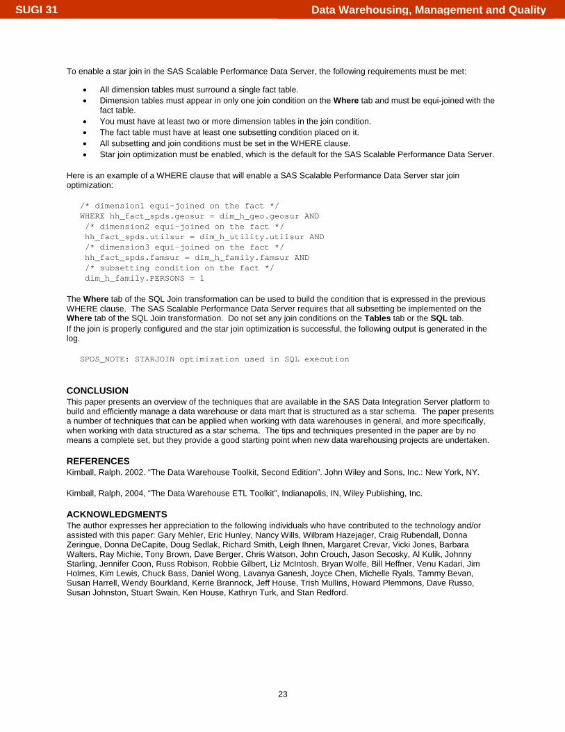
To enable a star join in the SAS Scalable Performance Data Server, the following requirements must be met:

• All dimension tables must surround a single fact table. • Dimension tables must appear in only one join condition on the Where tab and must be equi-joined with the

fact table. • You must have at least two or more dimension tables in the join condition. • The fact table must have at least one subsetting condition placed on it. • All subsetting and join conditions must be set in the WHERE clause. • Star join optimization must be enabled, which is the default for the SAS Scalable Performance Data Server.

Here is an example of a WHERE clause that will enable a SAS Scalable Performance Data Server star join optimization:

/* dimension1 equi-joined on the fact */ WHERE hh_fact_spds.geosur = dim_h_geo.geosur AND /* dimension2 equi-joined on the fact */ hh_fact_spds.utilsur = dim_h_utility.utilsur AND /* dimension3 equi-joined on the fact */ hh_fact_spds.famsur = dim_h_family.famsur AND /* subsetting condition on the fact */ dim_h_family.PERSONS = 1

The Where tab of the SQL Join transformation can be used to build the condition that is expressed in the previous WHERE clause. The SAS Scalable Performance Data Server requires that all subsetting be implemented on the Where tab of the SQL Join transformation. Do not set any join conditions on the Tables tab or the SQL tab. If the join is properly configured and the star join optimization is successful, the following output is generated in the log.

SPDS_NOTE: STARJOIN optimization used in SQL execution

CONCLUSION This paper presents an overview of the techniques that are available in the SAS Data Integration Server platform to build and efficiently manage a data warehouse or data mart that is structured as a star schema. The paper presents a number of techniques that can be applied when working with data warehouses in general, and more specifically, when working with data structured as a star schema. The tips and techniques presented in the paper are by no means a complete set, but they provide a good starting point when new data warehousing projects are undertaken.

REFERENCES Kimball, Ralph. 2002. “The Data Warehouse Toolkit, Second Edition”. John Wiley and Sons, Inc.: New York, NY. Kimball, Ralph, 2004, “The Data Warehouse ETL Toolkit”, Indianapolis, IN, Wiley Publishing, Inc.

ACKNOWLEDGMENTS The author expresses her appreciation to the following individuals who have contributed to the technology and/or assisted with this paper: Gary Mehler, Eric Hunley, Nancy Wills, Wilbram Hazejager, Craig Rubendall, Donna Zeringue, Donna DeCapite, Doug Sedlak, Richard Smith, Leigh Ihnen, Margaret Crevar, Vicki Jones, Barbara Walters, Ray Michie, Tony Brown, Dave Berger, Chris Watson, John Crouch, Jason Secosky, Al Kulik, Johnny Starling, Jennifer Coon, Russ Robison, Robbie Gilbert, Liz McIntosh, Bryan Wolfe, Bill Heffner, Venu Kadari, Jim Holmes, Kim Lewis, Chuck Bass, Daniel Wong, Lavanya Ganesh, Joyce Chen, Michelle Ryals, Tammy Bevan, Susan Harrell, Wendy Bourkland, Kerrie Brannock, Jeff House, Trish Mullins, Howard Plemmons, Dave Russo, Susan Johnston, Stuart Swain, Ken House, Kathryn Turk, and Stan Redford.


24

RESOURCES Mehler, Gary. 2005. “Best Practices in Enterprise Data Management”, Proceedings of the Thirtieth Annual SAS Users Group International Conference, Philadelphia, PA, SAS Institute Inc. Available www2.sas.com/proceedings/sugi30/098-30.pdf. SAS Institute. SAS OnlineDoc. Available support.sas.com/publishing/cdrom/index.html. SAS Institute. 2004. SAS 9.1.3 Open Metadata Architecture: Best Practices Guide, Cary, NC: SAS Institute Inc. SAS Institute. 2004. SAS 9.1 Open Metadata Interface: User’s Guide, Cary, NC: SAS Institute Inc. SAS Institute. 2004. SAS 9.1 Open Metadata Interface: Reference, Cary, NC: SAS Institute Inc. Secosky, Jason. 2004. “The DATA step in SAS®9: What’s New?.” Base SAS Community. SAS Institute Inc. Available support.sas.com/rnd/base/topics/datastep/dsv9-sugi-v3.pdf.

CONTACT INFORMATION Your comments and questions are valued and encouraged. Contact the author:

Nancy Rausch SAS Institute Inc. SAS Campus Drive Cary, NC 27513 Phone: (919) 531-8000 E-mail: [email protected] www.sas.com

SAS and all other SAS Institute Inc. product or service names are registered trademarks or trademarks of SAS Institute Inc. in the USA and other countries. ® indicates USA registration. Other brand and product names are trademarks of their respective companies.


http://www2.sas.com/proceedings/sugi30/098-30.pdf

http://support.sas.com/publishing/cdrom/index.html

http://support.sas.com/rnd/base/topics/datastep/dsv9-sugi-v3.pdf

mailto:[email protected]

http://www.sas.com

096-31

Documents