1 1 comp5331: knowledge discovery and data minig instructor: lei chen acknowledgement: slides...

11

COMP5331: Knowledge Discovery and Data

Minig

Instructor: Lei Chen

Acknowledgement: Slides modified by Dr. Lei Chen based on the slides provided by Jiawei Han, Micheline

Kamber, and Jian Pei

©2012 Han, Kamber & Pei. All rights reserved.

2

Chapter 2: Getting to Know Your Data

Data Objects and Attribute Types

Basic Statistical Descriptions of Data

Measuring Data Similarity and Dissimilarity

Summary

3

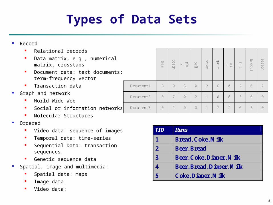
Types of Data Sets

Record Relational records Data matrix, e.g., numerical matrix,

crosstabs Document data: text documents: term-

frequency vector Transaction data

Graph and network World Wide Web Social or information networks Molecular Structures

Ordered Video data: sequence of images Temporal data: time-series Sequential Data: transaction

sequences Genetic sequence data

Spatial, image and multimedia: Spatial data: maps Image data: Video data:

Document 1

season

timeout

lost

win

game

score

ball

play

coach

team

Document 2

Document 3

3 0 5 0 2 6 0 2 0 2

0

0

7 0 2 1 0 0 3 0 0

1 0 0 1 2 2 0 3 0

TID Items

1 Bread, Coke, Milk

2 Beer, Bread

3 Beer, Coke, Diaper, Milk

4 Beer, Bread, Diaper, Milk

5 Coke, Diaper, Milk

4

Important Characteristics of Structured Data

Dimensionality Curse of dimensionality

Sparsity Only presence counts

Resolution

Patterns depend on the scale Distribution

Centrality and dispersion

5

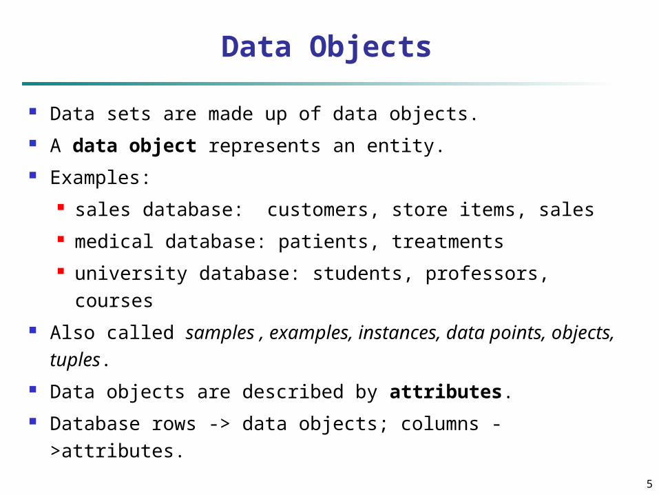
Data Objects

Data sets are made up of data objects. A data object represents an entity. Examples:

sales database: customers, store items, sales medical database: patients, treatments university database: students, professors, courses

Also called samples , examples, instances, data points, objects, tuples.

Data objects are described by attributes. Database rows -> data objects; columns -

>attributes.

6

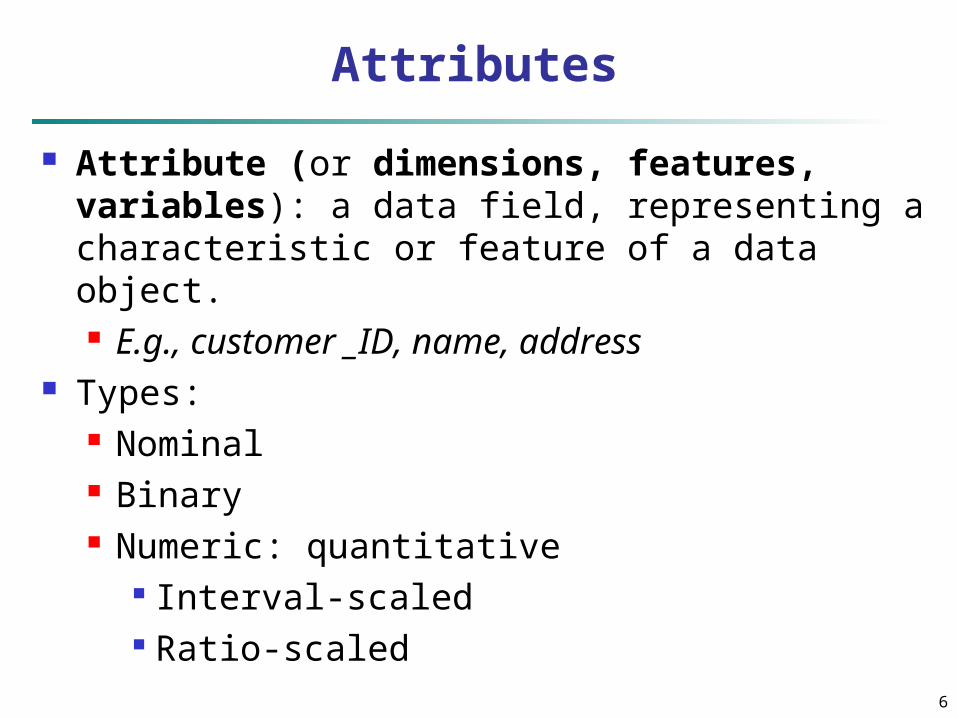
Attributes

Attribute (or dimensions, features, variables): a data field, representing a characteristic or feature of a data object. E.g., customer _ID, name, address

Types: Nominal Binary Numeric: quantitative

Interval-scaled Ratio-scaled

7

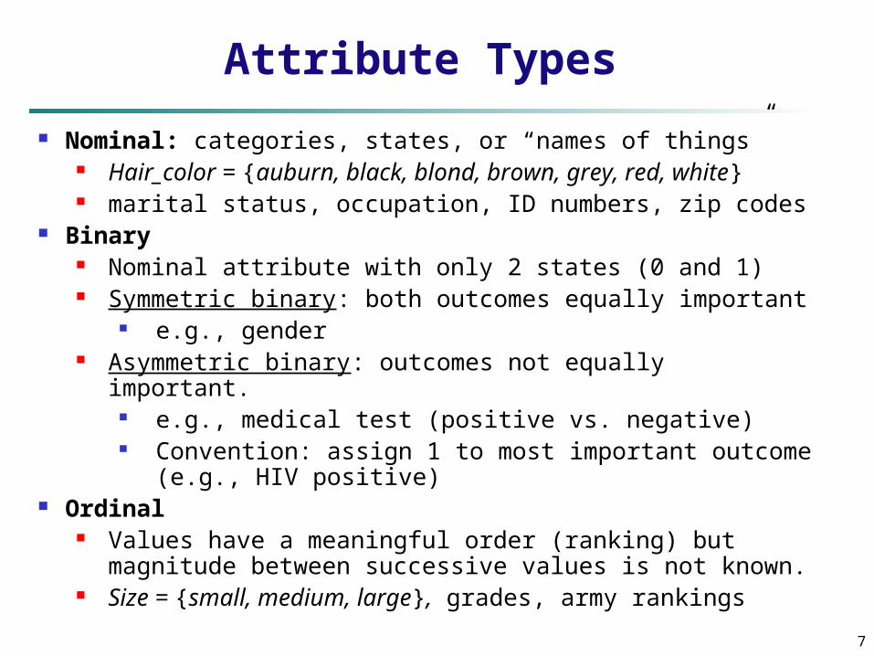
Attribute Types

Nominal: categories, states, or “names of things” Hair_color = {auburn, black, blond, brown, grey, red,

white} marital status, occupation, ID numbers, zip codes

Binary Nominal attribute with only 2 states (0 and 1) Symmetric binary: both outcomes equally important

e.g., gender Asymmetric binary: outcomes not equally important.

e.g., medical test (positive vs. negative) Convention: assign 1 to most important outcome

(e.g., HIV positive) Ordinal

Values have a meaningful order (ranking) but magnitude between successive values is not known.

Size = {small, medium, large}, grades, army rankings

8

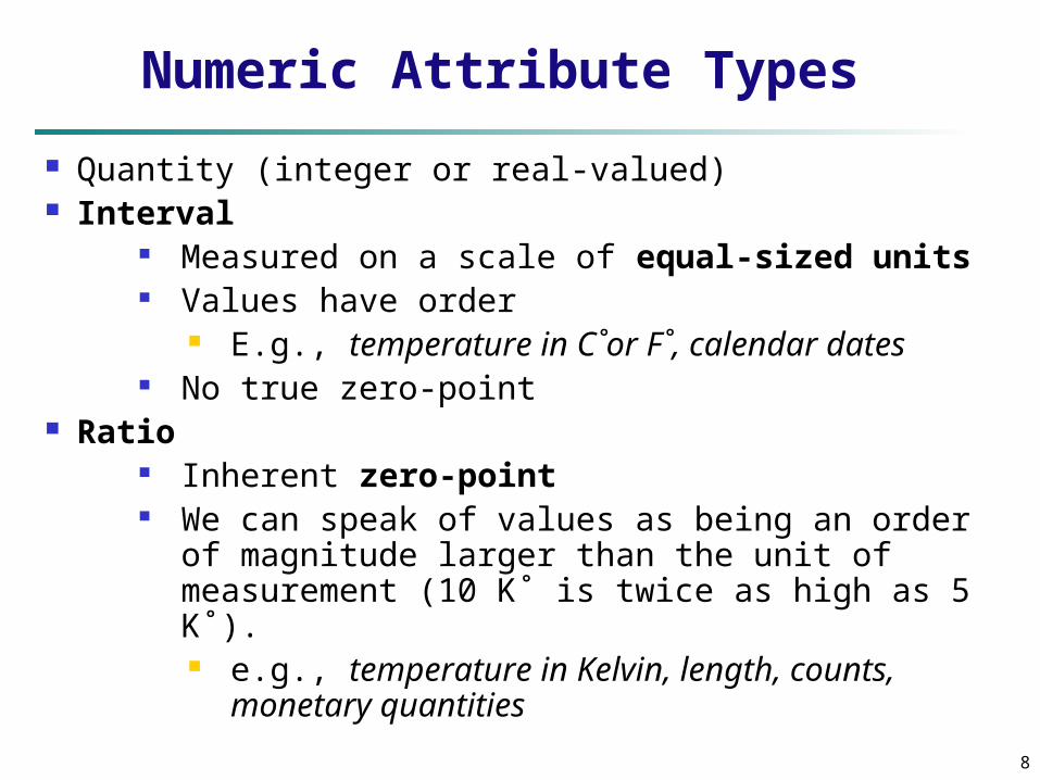
Numeric Attribute Types

Quantity (integer or real-valued) Interval

Measured on a scale of equal-sized units Values have order

E.g., temperature in C˚or F˚, calendar dates No true zero-point

Ratio Inherent zero-point We can speak of values as being an order of

magnitude larger than the unit of measurement (10 K˚ is twice as high as 5 K˚). e.g., temperature in Kelvin, length, counts,

monetary quantities

9

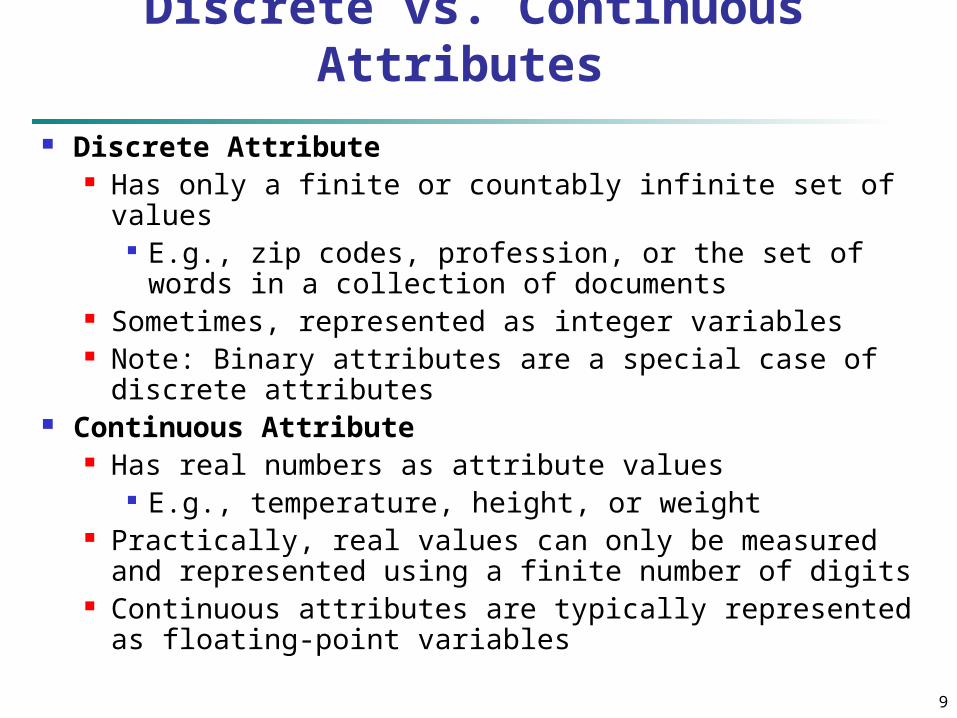
Discrete vs. Continuous Attributes

Discrete Attribute Has only a finite or countably infinite set of values

E.g., zip codes, profession, or the set of words in a collection of documents

Sometimes, represented as integer variables Note: Binary attributes are a special case of

discrete attributes Continuous Attribute

Has real numbers as attribute values E.g., temperature, height, or weight

Practically, real values can only be measured and represented using a finite number of digits

Continuous attributes are typically represented as floating-point variables

10





Summary

11


Motivation To better understand the data: central tendency,

variation and spread Data dispersion characteristics

median, max, min, quantiles, outliers, variance, etc. Numerical dimensions correspond to sorted intervals

Data dispersion: analyzed with multiple granularities of precision

Boxplot or quantile analysis on sorted intervals Dispersion analysis on computed measures

Folding measures into numerical dimensions Boxplot or quantile analysis on the transformed

cube

12

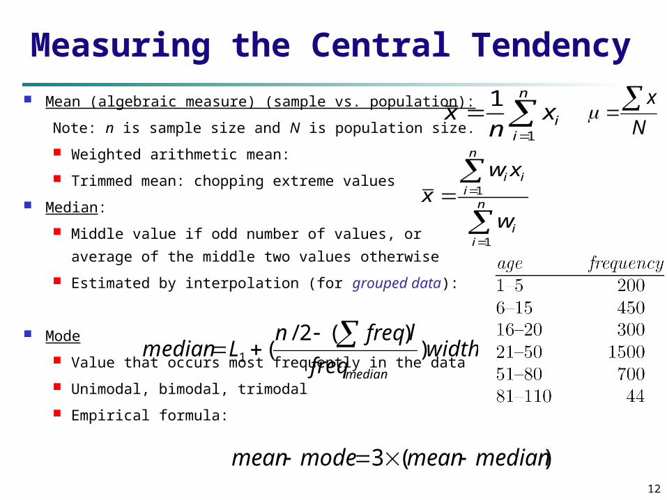
Measuring the Central Tendency

Mean (algebraic measure) (sample vs. population):

Note: n is sample size and N is population size.

Weighted arithmetic mean:

Trimmed mean: chopping extreme values

Median:

Middle value if odd number of values, or average

of the middle two values otherwise

Estimated by interpolation (for grouped data):

Mode

Value that occurs most frequently in the data

Unimodal, bimodal, trimodal

Empirical formula:

n

iix

nx

1

1

n

ii

n

iii

w

xwx

1

1

widthfreq

lfreqnLmedian

median

))(2/

(1

)(3 medianmeanmodemean

N

x

April 19, 2023 Data Mining: Concepts and Techniques 13

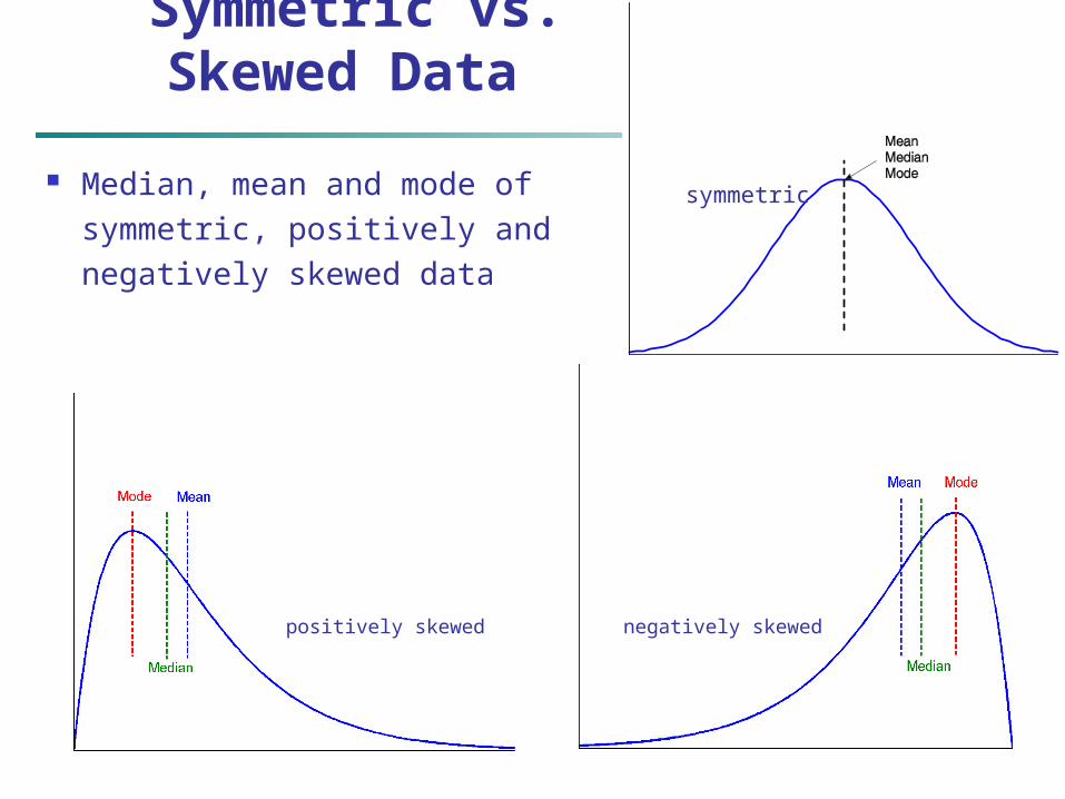
Symmetric vs. Skewed Data

Median, mean and mode of symmetric, positively and negatively skewed data

positively skewed negatively skewed

symmetric

14

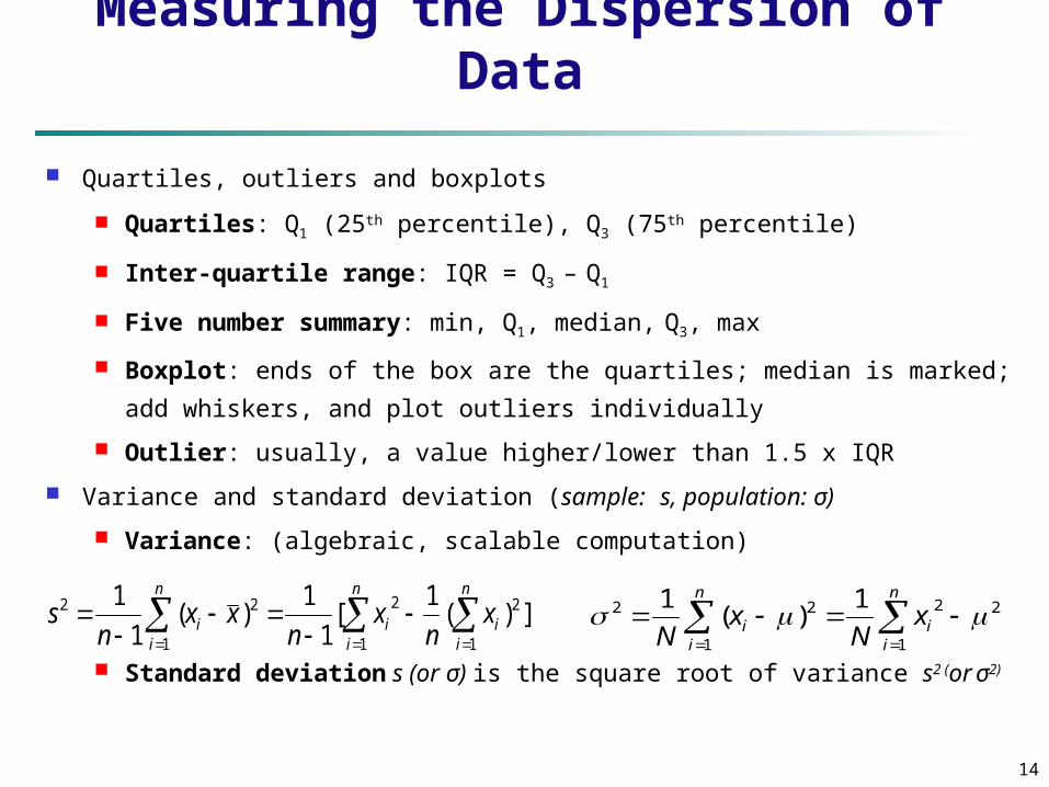
Measuring the Dispersion of Data

Quartiles, outliers and boxplots

Quartiles: Q1 (25th percentile), Q3 (75th percentile)

Inter-quartile range: IQR = Q3 – Q1

Five number summary: min, Q1, median, Q3, max

Boxplot: ends of the box are the quartiles; median is marked; add

whiskers, and plot outliers individually

Outlier: usually, a value higher/lower than 1.5 x IQR

Variance and standard deviation (sample: s, population: σ)

Variance: (algebraic, scalable computation)

Standard deviation s (or σ) is the square root of variance s2 (or σ2)

n

i

n

iii

n

ii x

nx

nxx

ns

1 1

22

1

22 ])(1

[1

1)(

1

1

n

ii

n

ii x

Nx

N 1

22

1

22 1)(

1

15

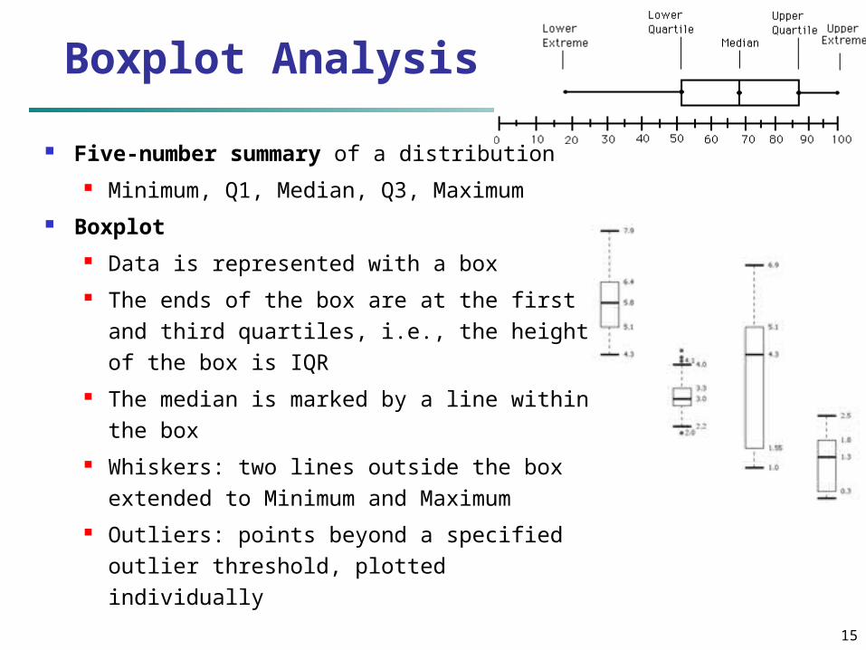
Boxplot Analysis

Five-number summary of a distribution Minimum, Q1, Median, Q3, Maximum

Boxplot Data is represented with a box The ends of the box are at the first and

third quartiles, i.e., the height of the box is IQR

The median is marked by a line within the box

Whiskers: two lines outside the box extended to Minimum and Maximum

Outliers: points beyond a specified outlier threshold, plotted individually

April 19, 2023 Data Mining: Concepts and Techniques 16

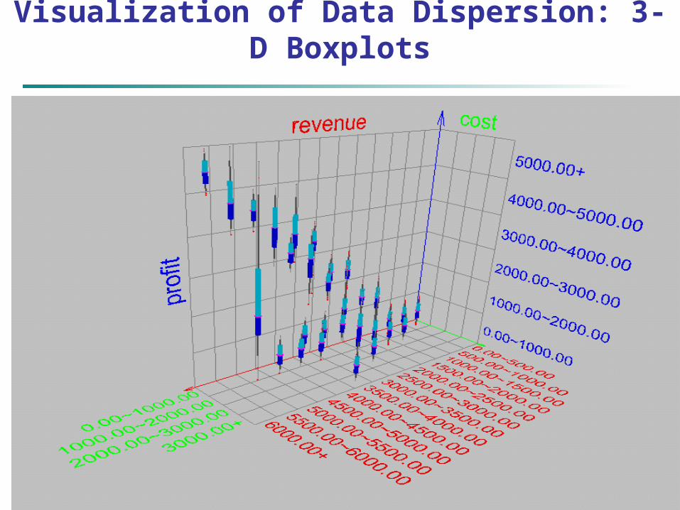
Visualization of Data Dispersion: 3-D Boxplots

17

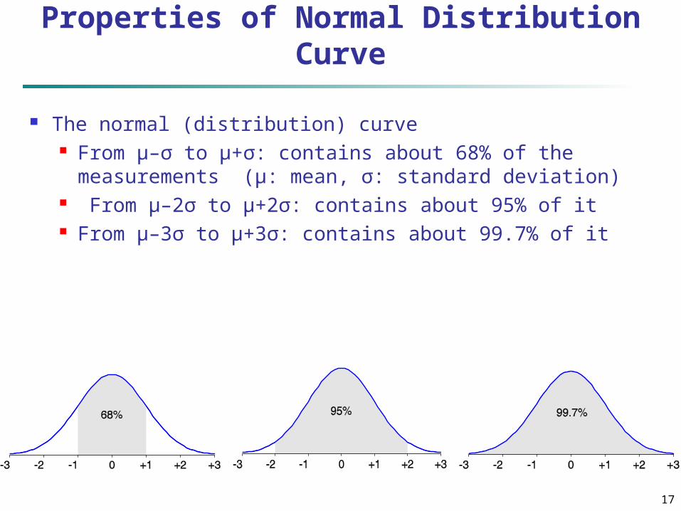
Properties of Normal Distribution Curve

The normal (distribution) curve From μ–σ to μ+σ: contains about 68% of the

measurements (μ: mean, σ: standard deviation) From μ–2σ to μ+2σ: contains about 95% of it From μ–3σ to μ+3σ: contains about 99.7% of it

18

Graphic Displays of Basic Statistical Descriptions

Boxplot: graphic display of five-number summary

Histogram: x-axis are values, y-axis repres.

frequencies

Quantile plot: each value xi is paired with fi indicating

that approximately 100 fi % of data are xi

Quantile-quantile (q-q) plot: graphs the quantiles of

one univariant distribution against the corresponding

quantiles of another

Scatter plot: each pair of values is a pair of

coordinates and plotted as points in the plane

19

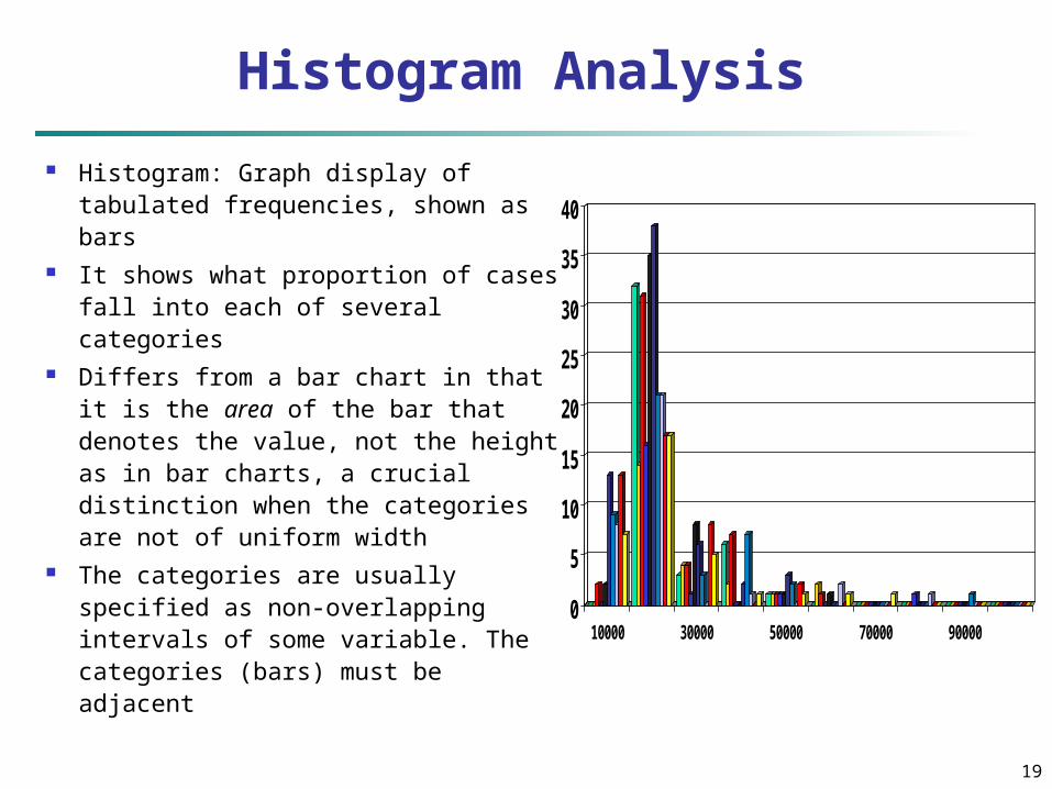
Histogram Analysis

Histogram: Graph display of tabulated frequencies, shown as bars

It shows what proportion of cases fall into each of several categories

Differs from a bar chart in that it is the area of the bar that denotes the value, not the height as in bar charts, a crucial distinction when the categories are not of uniform width

The categories are usually specified as non-overlapping intervals of some variable. The categories (bars) must be adjacent

0

5

10

15

20

25

30

35

40

10000 30000 50000 70000 90000

20

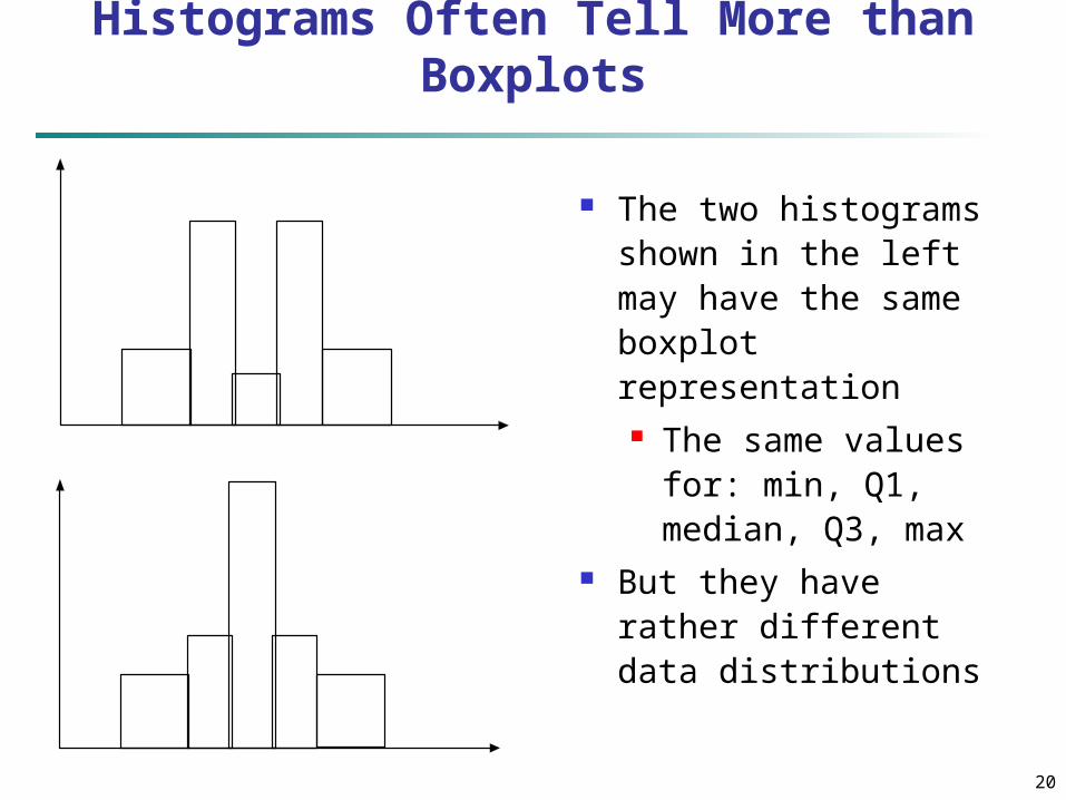
Histograms Often Tell More than Boxplots

The two histograms shown in the left may have the same boxplot representation The same values

for: min, Q1, median, Q3, max

But they have rather different data distributions

Data Mining: Concepts and Techniques 21

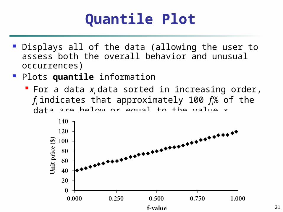
Quantile Plot

Displays all of the data (allowing the user to assess both the overall behavior and unusual occurrences)

Plots quantile information For a data xi data sorted in increasing order, fi

indicates that approximately 100 fi% of the data are below or equal to the value xi

22

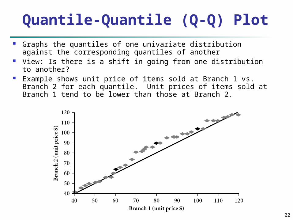
Quantile-Quantile (Q-Q) Plot Graphs the quantiles of one univariate distribution against the

corresponding quantiles of another View: Is there is a shift in going from one distribution to another? Example shows unit price of items sold at Branch 1 vs. Branch 2

for each quantile. Unit prices of items sold at Branch 1 tend to be lower than those at Branch 2.

23

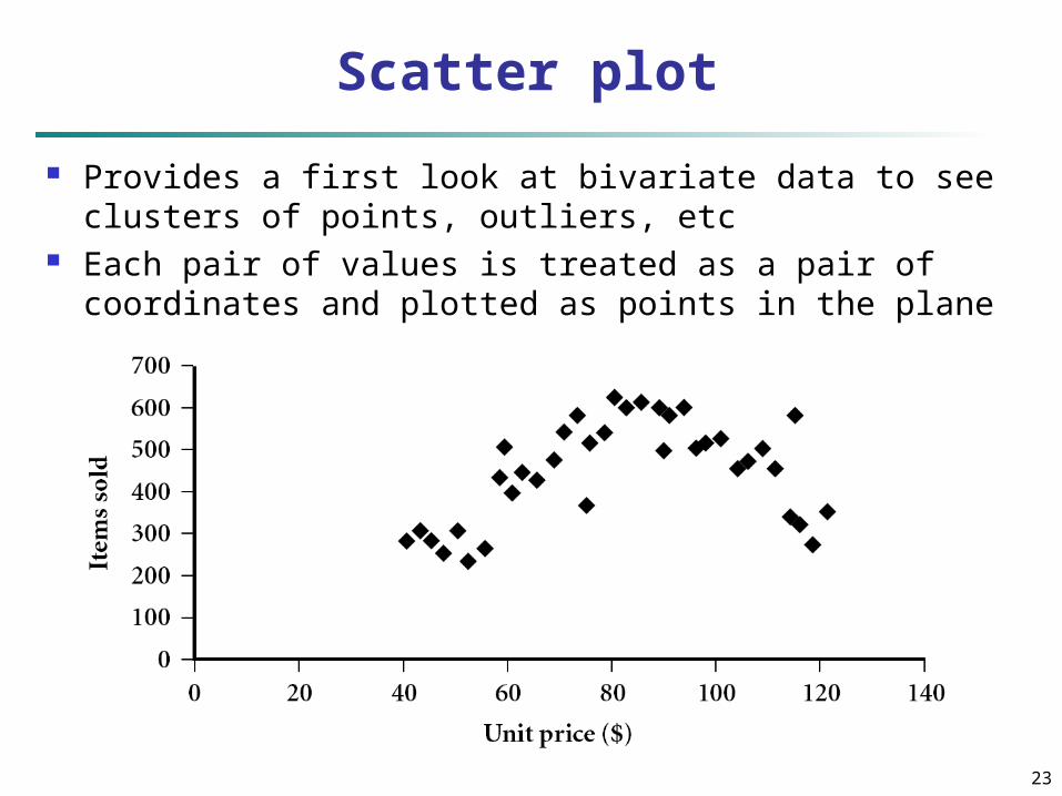
Scatter plot

Provides a first look at bivariate data to see clusters of points, outliers, etc

Each pair of values is treated as a pair of coordinates and plotted as points in the plane

24

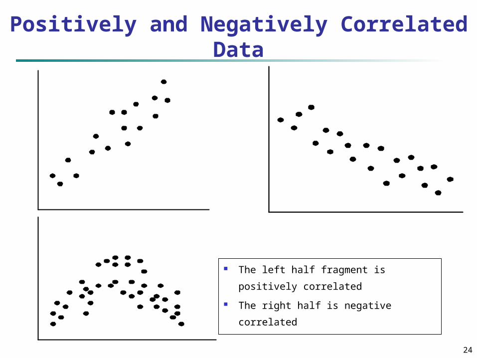
Positively and Negatively Correlated Data

The left half fragment is positively

correlated

The right half is negative correlated

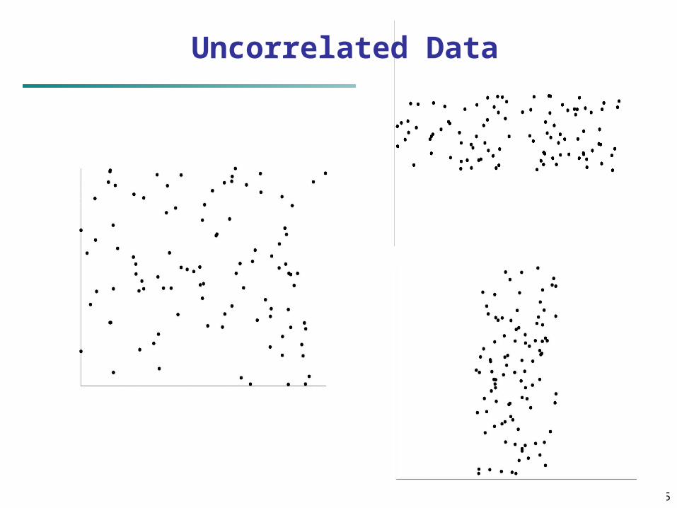
25

Uncorrelated Data

26





Summary

27

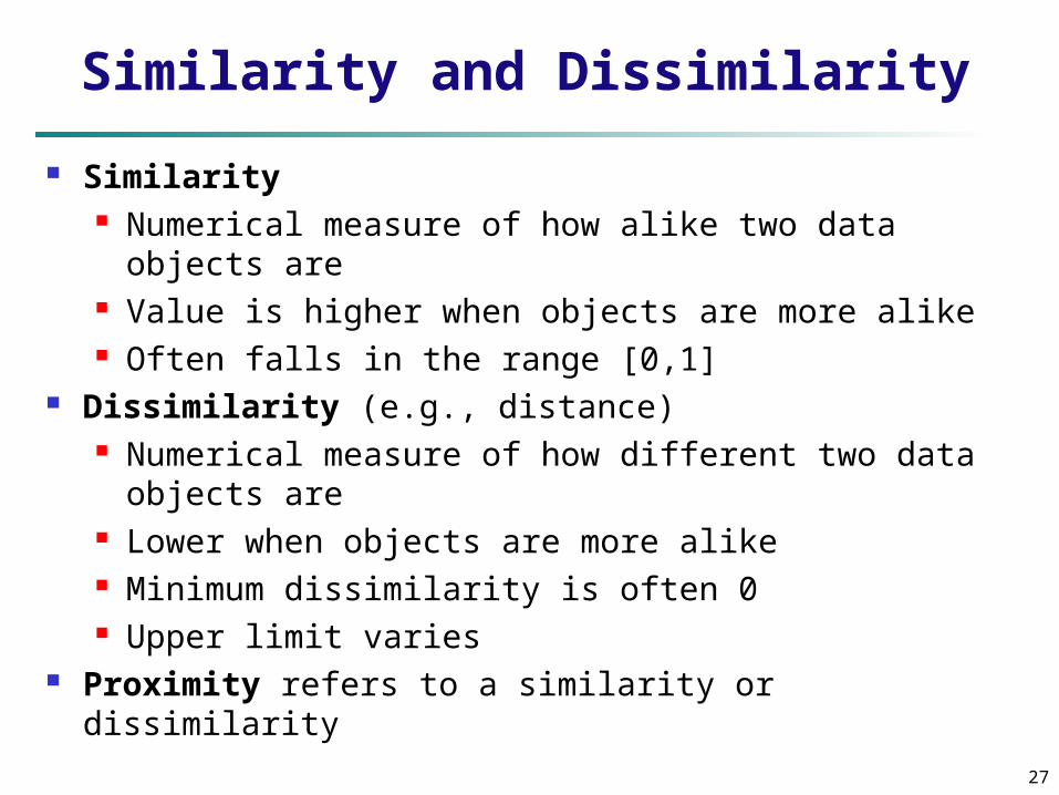
Similarity and Dissimilarity

Similarity Numerical measure of how alike two data objects

are Value is higher when objects are more alike Often falls in the range [0,1]

Dissimilarity (e.g., distance) Numerical measure of how different two data

objects are Lower when objects are more alike Minimum dissimilarity is often 0 Upper limit varies

Proximity refers to a similarity or dissimilarity

28

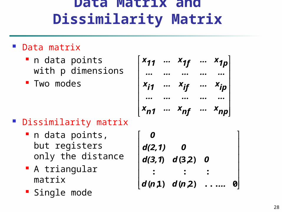
Data Matrix and Dissimilarity Matrix

Data matrix n data points with

p dimensions Two modes

Dissimilarity matrix n data points, but

registers only the distance

A triangular matrix Single mode

npx...nfx...n1x

...............ipx...ifx...i1x

...............1px...1fx...11x

0...)2,()1,(

:::

)2,3()

...ndnd

0dd(3,1

0d(2,1)

0

29

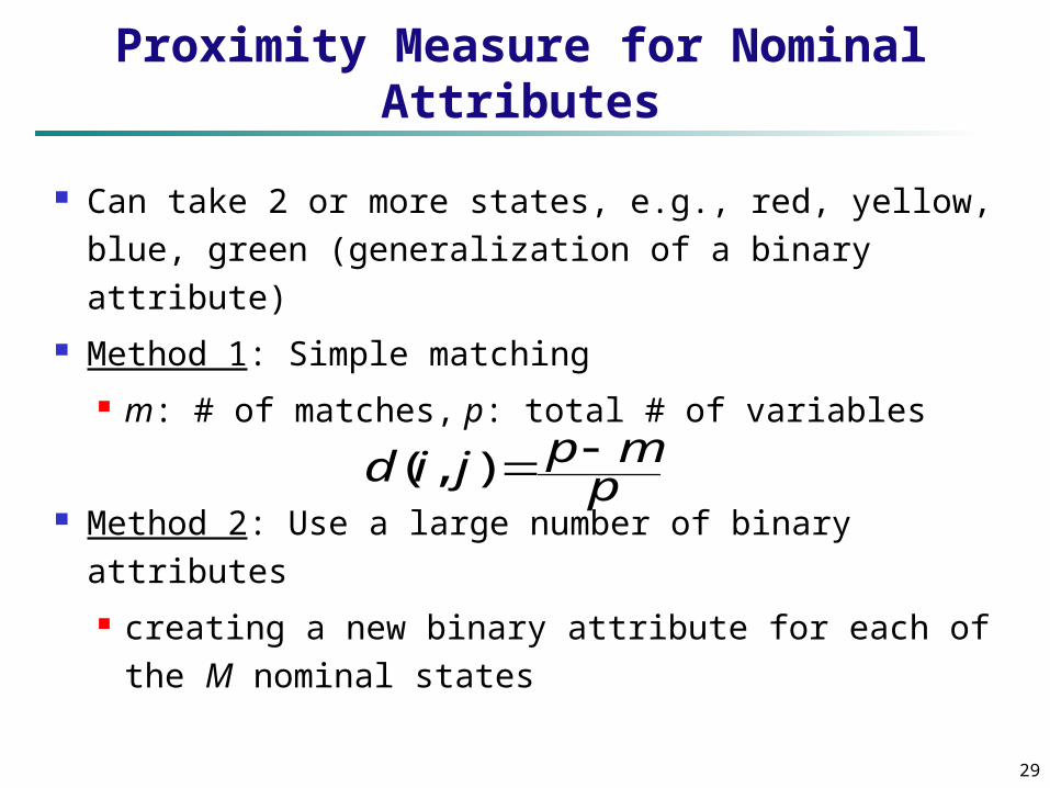
Proximity Measure for Nominal Attributes

Can take 2 or more states, e.g., red, yellow, blue, green (generalization of a binary attribute)

Method 1: Simple matching m: # of matches, p: total # of variables

Method 2: Use a large number of binary attributes creating a new binary attribute for each of the

M nominal states

pmpjid ),(

30

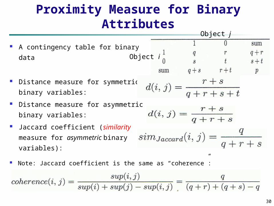
Proximity Measure for Binary Attributes

A contingency table for binary data

Distance measure for symmetric

binary variables:

Distance measure for asymmetric

binary variables:

Jaccard coefficient (similarity

measure for asymmetric binary

variables):

Note: Jaccard coefficient is the same as “coherence”:

Object i

Object j

31

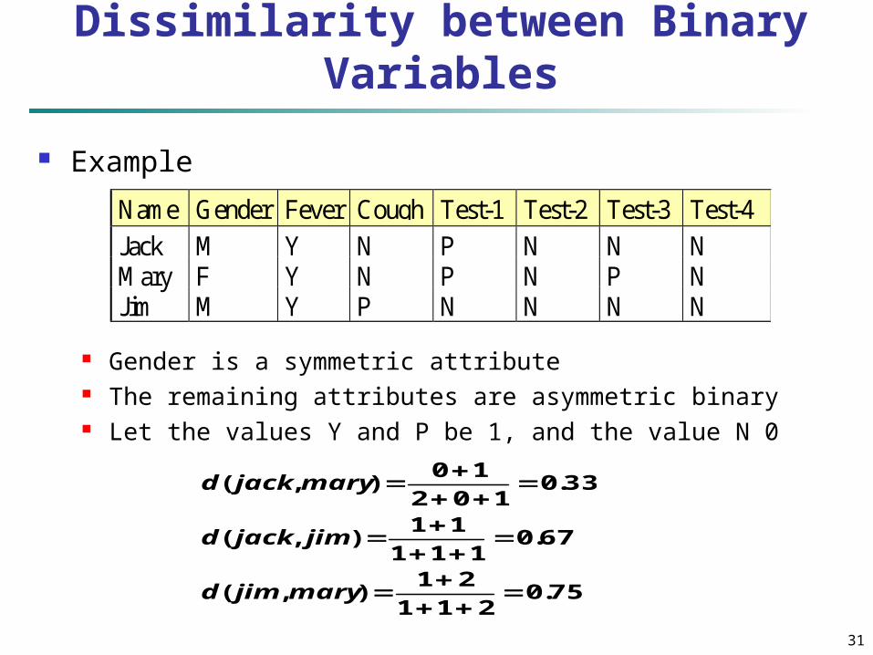
Dissimilarity between Binary Variables

Example

Gender is a symmetric attribute The remaining attributes are asymmetric binary Let the values Y and P be 1, and the value N 0

Name Gender Fever Cough Test-1 Test-2 Test-3 Test-4

Jack M Y N P N N NMary F Y N P N P NJim M Y P N N N N

75.0211

21),(

67.0111

11),(

33.0102

10),(

maryjimd

jimjackd

maryjackd

32

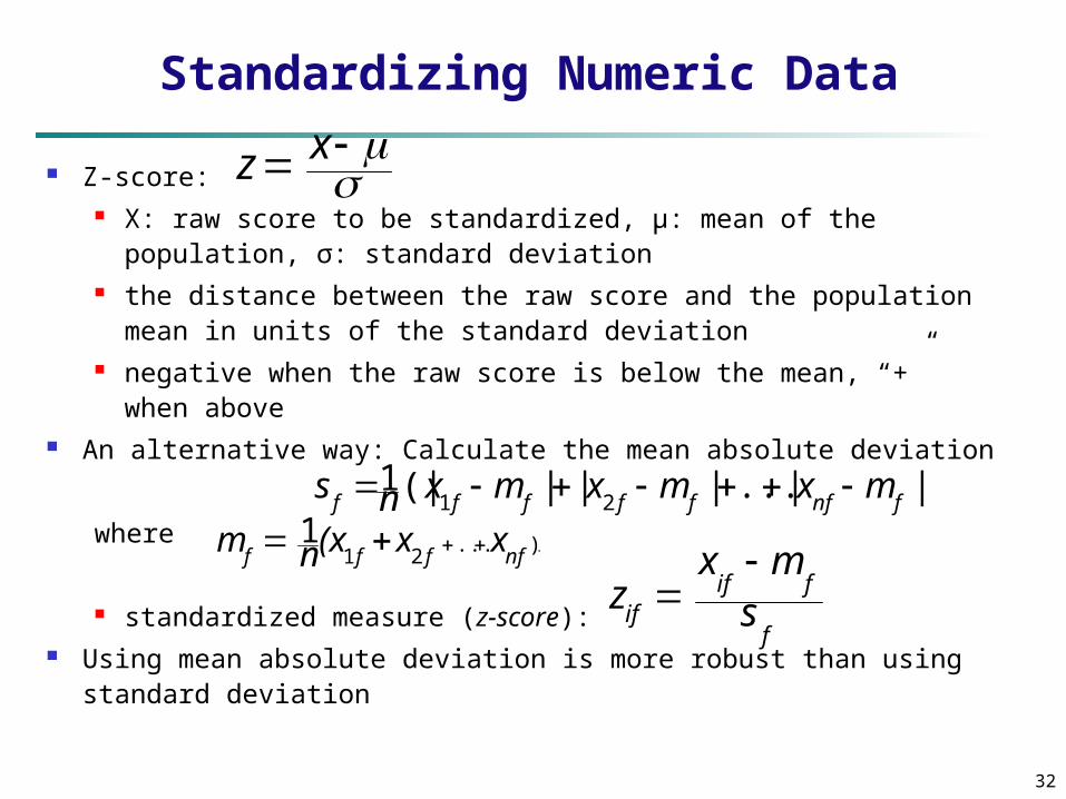
Standardizing Numeric Data

Z-score: X: raw score to be standardized, μ: mean of the

population, σ: standard deviation the distance between the raw score and the population

mean in units of the standard deviation negative when the raw score is below the mean, “+”

when above An alternative way: Calculate the mean absolute deviation

where

standardized measure (z-score): Using mean absolute deviation is more robust than using

standard deviation

.)...21

1nffff

xx(xn m |)|...|||(|1

21 fnffffffmxmxmxns

f

fifif s

mx z

x z

33

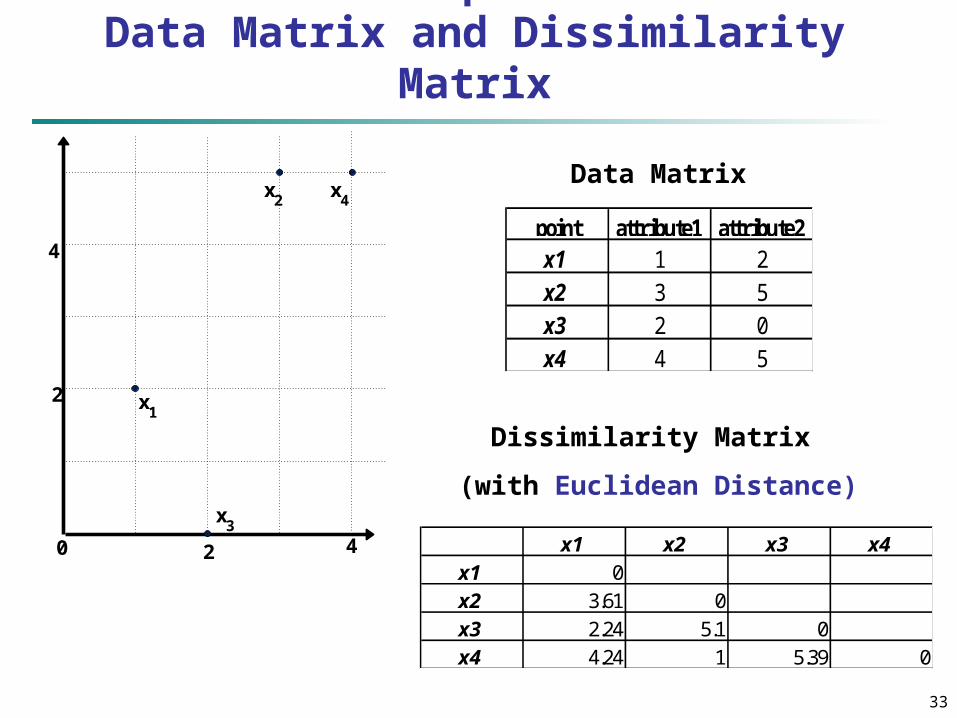
Example: Data Matrix and Dissimilarity Matrix

point attribute1 attribute2x1 1 2x2 3 5x3 2 0x4 4 5

Dissimilarity Matrix

(with Euclidean Distance)

x1 x2 x3 x4

x1 0

x2 3.61 0

x3 2.24 5.1 0

x4 4.24 1 5.39 0

Data Matrix

0 2 4

2

4

x1

x2

x3

x4

34

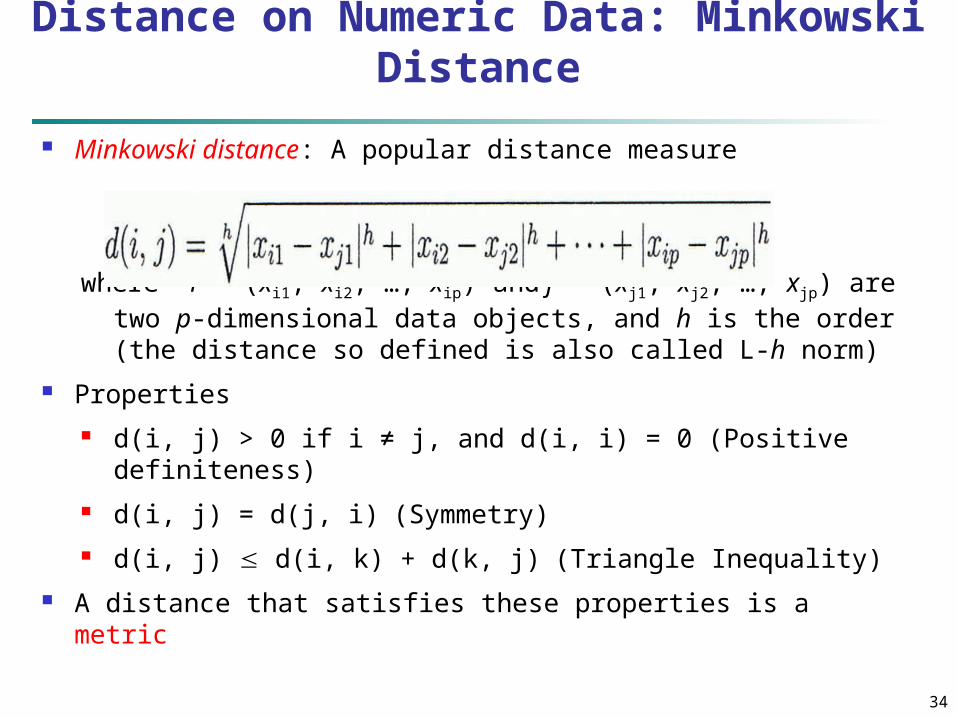
Distance on Numeric Data: Minkowski Distance

Minkowski distance: A popular distance measure

where i = (xi1, xi2, …, xip) and j = (xj1, xj2, …, xjp) are two p-dimensional data objects, and h is the order (the distance so defined is also called L-h norm)

Properties d(i, j) > 0 if i ≠ j, and d(i, i) = 0 (Positive definiteness) d(i, j) = d(j, i) (Symmetry) d(i, j) d(i, k) + d(k, j) (Triangle Inequality)

A distance that satisfies these properties is a metric

35

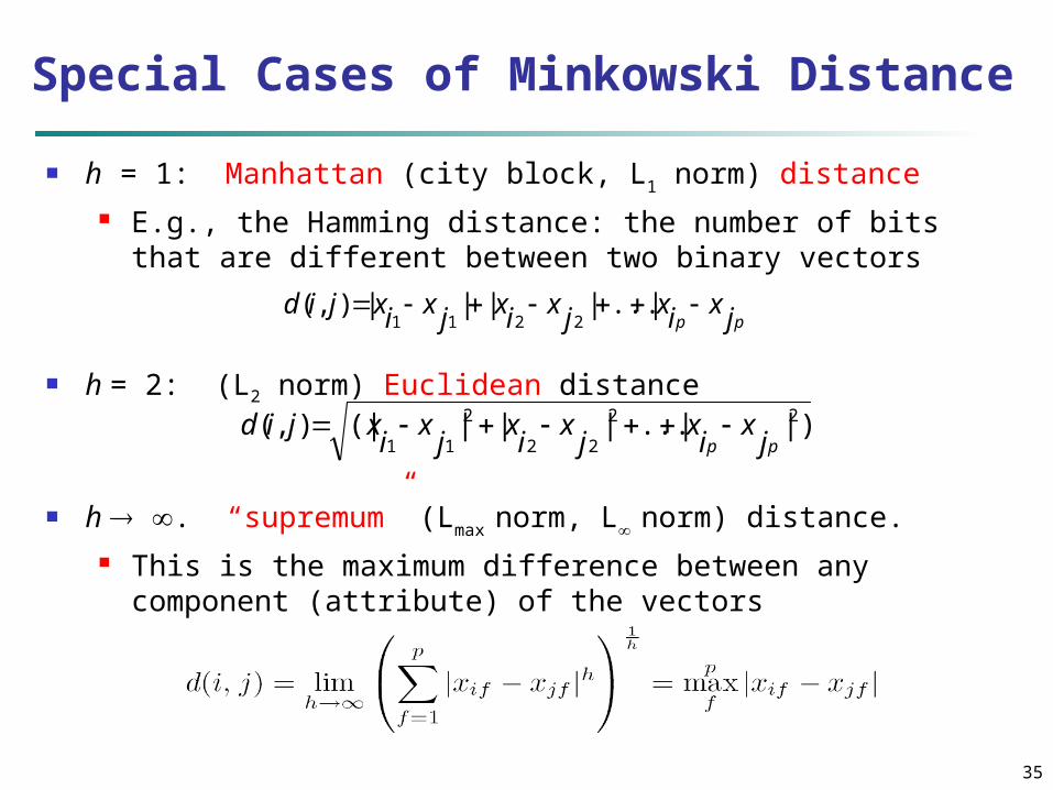
Special Cases of Minkowski Distance

h = 1: Manhattan (city block, L1 norm) distance E.g., the Hamming distance: the number of bits that are

different between two binary vectors

h = 2: (L2 norm) Euclidean distance

h . “supremum” (Lmax norm, L norm) distance. This is the maximum difference between any component

(attribute) of the vectors

)||...|||(|),( 22

22

2

11 pp jx

ix

jx

ix

jx

ixjid

||...||||),(2211 pp jxixjxixjxixjid

36

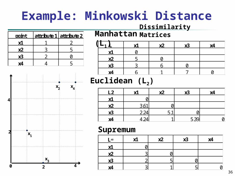
Example: Minkowski DistanceDissimilarity Matrices

point attribute 1 attribute 2x1 1 2x2 3 5x3 2 0x4 4 5

L x1 x2 x3 x4x1 0x2 5 0x3 3 6 0x4 6 1 7 0

L2 x1 x2 x3 x4x1 0x2 3.61 0x3 2.24 5.1 0x4 4.24 1 5.39 0

L x1 x2 x3 x4

x1 0x2 3 0x3 2 5 0x4 3 1 5 0

Manhattan (L1)

Euclidean (L2)

Supremum

0 2 4

2

4

x1

x2

x3

x4

37

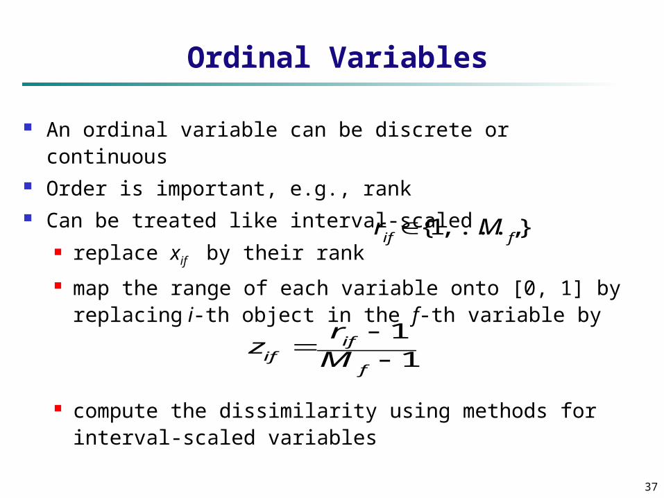
Ordinal Variables

An ordinal variable can be discrete or continuous Order is important, e.g., rank Can be treated like interval-scaled

replace xif by their rank

map the range of each variable onto [0, 1] by replacing i-th object in the f-th variable by

compute the dissimilarity using methods for interval-scaled variables

11

f

ifif M

rz

},...,1{fif

Mr

38

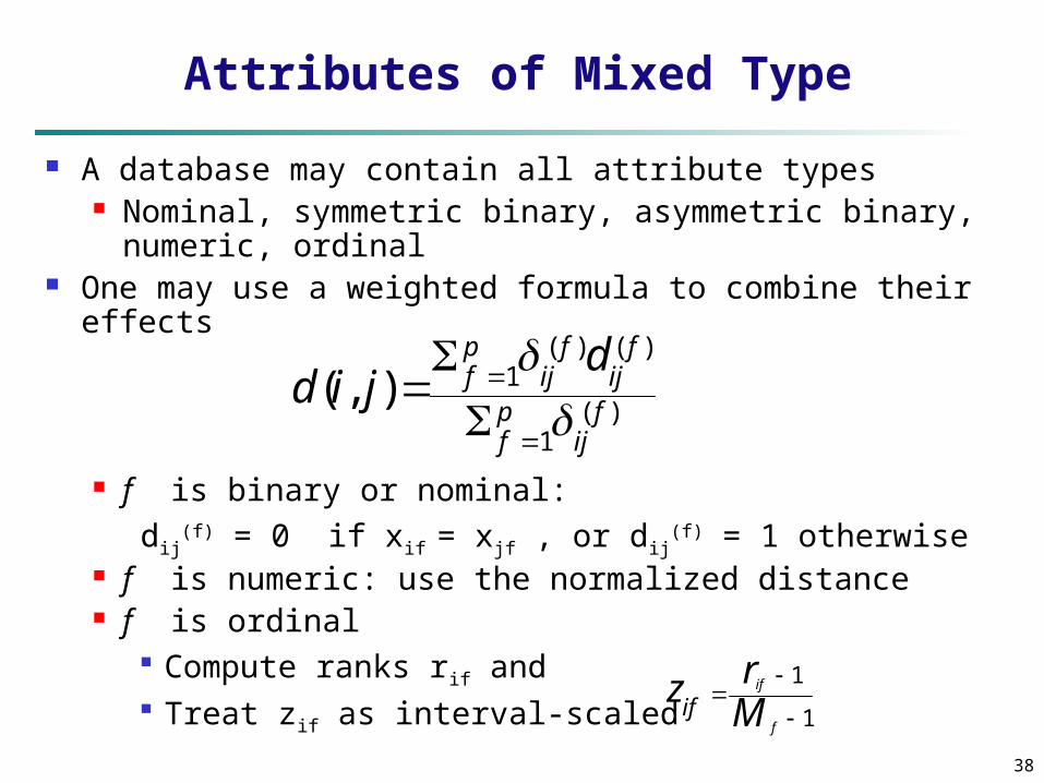
Attributes of Mixed Type

A database may contain all attribute types Nominal, symmetric binary, asymmetric binary,

numeric, ordinal One may use a weighted formula to combine their

effects

f is binary or nominal:dij

(f) = 0 if xif = xjf , or dij(f) = 1 otherwise

f is numeric: use the normalized distance f is ordinal

Compute ranks rif and Treat zif as interval-scaled

)(1

)()(1),(

fij

pf

fij

fij

pf

djid

1

1

f

if

Mrz

if

39

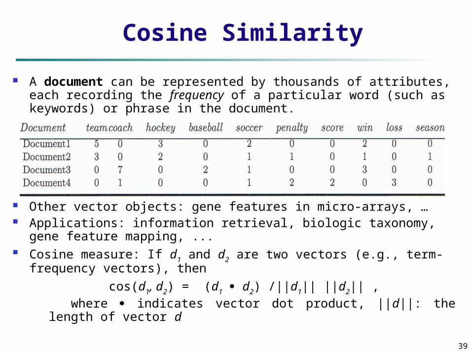
Cosine Similarity

A document can be represented by thousands of attributes, each recording the frequency of a particular word (such as keywords) or phrase in the document.

Other vector objects: gene features in micro-arrays, … Applications: information retrieval, biologic taxonomy, gene

feature mapping, ... Cosine measure: If d1 and d2 are two vectors (e.g., term-frequency

vectors), then

cos(d1, d2) = (d1 d2) /||d1|| ||d2|| , where indicates vector dot product, ||d||: the length of vector

d

40

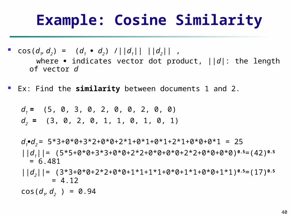
Example: Cosine Similarity

cos(d1, d2) = (d1 d2) /||d1|| ||d2|| , where indicates vector dot product, ||d|: the length of vector d

Ex: Find the similarity between documents 1 and 2.

d1 = (5, 0, 3, 0, 2, 0, 0, 2, 0, 0)

d2 = (3, 0, 2, 0, 1, 1, 0, 1, 0, 1)

d1d2 = 5*3+0*0+3*2+0*0+2*1+0*1+0*1+2*1+0*0+0*1 = 25

||d1||= (5*5+0*0+3*3+0*0+2*2+0*0+0*0+2*2+0*0+0*0)0.5=(42)0.5 = 6.481

||d2||= (3*3+0*0+2*2+0*0+1*1+1*1+0*0+1*1+0*0+1*1)0.5=(17)0.5 = 4.12

cos(d1, d2 ) = 0.94

41




Data Visualization


Summary

Summary Data attribute types: nominal, binary, ordinal, interval-scaled,

ratio-scaled Many types of data sets, e.g., numerical, text, graph, Web,

image. Gain insight into the data by:

Basic statistical data description: central tendency, dispersion, graphical displays

Data visualization: map data onto graphical primitives Measure data similarity

Above steps are the beginning of data preprocessing. Many methods have been developed but still an active area of

research.

References W. Cleveland, Visualizing Data, Hobart Press, 1993 T. Dasu and T. Johnson. Exploratory Data Mining and Data Cleaning.

John Wiley, 2003 U. Fayyad, G. Grinstein, and A. Wierse. Information Visualization in

Data Mining and Knowledge Discovery, Morgan Kaufmann, 2001 L. Kaufman and P. J. Rousseeuw. Finding Groups in Data: an

Introduction to Cluster Analysis. John Wiley & Sons, 1990. H. V. Jagadish et al., Special Issue on Data Reduction Techniques.

Bulletin of the Tech. Committee on Data Eng., 20(4), Dec. 1997 D. A. Keim. Information visualization and visual data mining, IEEE

trans. on Visualization and Computer Graphics, 8(1), 2002 D. Pyle. Data Preparation for Data Mining. Morgan Kaufmann, 1999 S. Santini and R. Jain,” Similarity measures”, IEEE Trans. on Pattern

Analysis and Machine Intelligence, 21(9), 1999 E. R. Tufte. The Visual Display of Quantitative Information, 2nd ed.,

Graphics Press, 2001 C. Yu et al., Visual data mining of multimedia data for social and

behavioral studies, Information Visualization, 8(1), 2009

1 1 comp5331: knowledge discovery and data minig instructor: lei chen acknowledgement: slides...

Documents

data data objects

data objects data sets

spatial data

video data

data field

data points

maps image data

data minig instructor