1 1 Slide

Slide

| | | | | | | | | | | |

|

|

| |

|

|

|

|

| |

|

|

|UCL

CL

LCL

Chapter 13Statistical Methods for Quality Control

Statistical Process Control Acceptance Sampling

2 2 Slide

Slide

Quality Terminology

Quality is “the totality of features and characteristics of a product or service that bears on its ability to satisfy given needs.”

Quality assurance refers to the entire system of policies, procedures, and guidelines established by an organization to achieve and maintain quality.

The objective of quality engineering is to include quality in the design of products and processes and to identify potential quality problems prior to production.

Quality control consists of making a series of inspections and measurements to determine whether quality standards are being met.

3 3 Slide

Slide

Statistical Process Control (SPC)

The goal of SPC is to determine whether the process can be continued or whether it should be adjusted to achieve a desired quality level.

If the variation in the quality of the production output is due to assignable causes (operator error, worn-out tooling, bad raw material, . . . ) the process should be adjusted or corrected as soon as possible.

If the variation in output is due to common causes (variation in materials, humidity, temperature, . . . ) which the manager cannot control, the process does not need to be adjusted.

4 4 Slide

Slide

SPC Hypotheses

SPC procedures are based on hypothesis-testing methodology.

The null hypothesis H0 is formulated in terms of the production process being in control.

The alternative hypothesis Ha is formulated in terms of the process being out of control.

As with other hypothesis-testing procedures, both a Type I error (adjusting an in-control process) and a Type II error (allowing an out-of-control process to continue) are possible.

5 5 Slide

Slide

The Outcomes of SPC

Type I and Type II Errors State of Production

Process

H0 True Ha True

Decision In Control Out of Control

Accept H0 Correct Type II

Continue Process DecisionError

Reject H0 Type I Correct

Adjust Process Error Decision

6 6 Slide

Slide

Control Charts

SPC uses graphical displays known as control charts to monitor a production process.

Control charts provide a basis for deciding whether the variation in the output is due to common causes (in control) or assignable causes (out of control).

Two important lines on a control chart are the upper control limit (UCL) and lower control limit (LCL).

These lines are chosen so that when the process is in control there will be a high probability that the sample finding will be between the two lines.

Values outside of the control limits provide strong evidence that the process is out of control.

7 7 Slide

Slide

Types of Control Charts

An x chart is used if the quality of the output is measured in terms of a variable such as length, weight, temperature, and so on.

x represents the mean value found in a sample of the output.

An R chart is used to monitor the range of the measurements in the sample.

A p chart is used to monitor the proportion defective in the sample.

An np chart is used to monitor the number of defective items in the sample.

8 8 Slide

Slide

Interpretation of Control Charts

The location and pattern of points in a control chart enable us to determine, with a small probability of error, whether a process is in statistical control.

A primary indication that a process may be out of control is a data point outside the control limits.

Certain patterns of points within the control limits can be warning signals of quality problems:• Large number of points on one side of

center line.• Six or seven points in a row that indicate

either an increasing or decreasing trend.• . . . and other patterns.

9 9 Slide

Slide

Control Limits for an x Chart

Process Mean and Standard Deviation Known

Process Mean and Standard Deviation Unknown

where:x = overall sample mean

R = average range A2 = a constant that depends on n; taken from

“Factors for Control Charts” table

UCL = 3 x

LCL = 3 x

UCL = x A R 2

LCL = x A R 2

=_

10 10 Slide

Slide

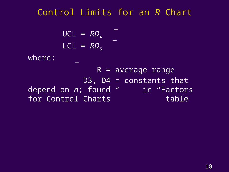
Control Limits for an R Chart

UCL = RD4

LCL = RD3

where:

R = average range D3, D4 = constants that depend on n; found in “Factors for Control Charts” table

_

_

_

11 11 Slide

Slide

Factors for x and R Control Charts

Factors Table (Partial)

n d2 A2 d3 D3 D4

. . . . . .6 2.534 0.483 0.848 0 2.0047 2.704 0.419 0.833 0.076 1.9248 2.847 0.373 0.820 0.136 1.8649 2.970 0.337 0.808 0.184 1.81610 3.078 0.308 0.797 0.223 1.777. . . . . .

12 12 Slide

Slide

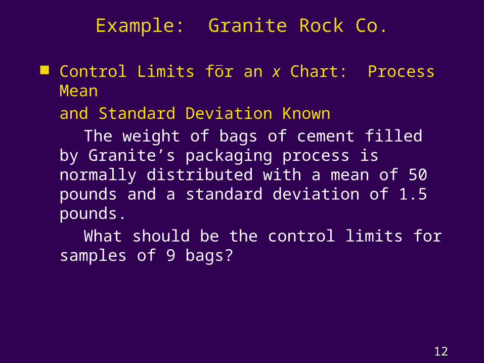
Example: Granite Rock Co.

Control Limits for an x Chart: Process Meanand Standard Deviation Known

The weight of bags of cement filled by Granite’s packaging process is normally distributed with a mean of 50 pounds and a standard deviation of 1.5 pounds.

What should be the control limits for samples of 9 bags?

13 13 Slide

Slide

Example: Granite Rock Co.

Control Limits for an x Chart: Process Meanand Standard Deviation Known

= 50, = 1.5, n = 9

UCL = 50 + 3(.5) = 51.5 LCL = 50 - 3(.5) = 48.5

x n 15

9 05. .

14 14 Slide

Slide

Example: Granite Rock Co.

Control Limits for x and R Charts: Process Meanand Standard Deviation Unknown

Suppose Granite does not know the true mean and standard deviation for its bag filling process. It wants to develop x and R charts based on forty samples of 9 bags each. The average of the sample means is 50.1 pounds and the average of the sample ranges is 3.25 pounds.

15 15 Slide

Slide

Example: Granite Rock Co.

Control Limits for x and R Charts: Process Meanand Standard Deviation Unknown

x = 50.1, R = 3.25, n = 9• R Chart

UCL = RD4 = 3.25(1.816) = 5.9

LCL = RD3 = 3.25(0.184) = 0.6• x Chart

UCL = x + A2R = 50.1 + .337(3.25) = 51.2

LCL = x - A2R = 50.1 - .337(3.25) = 49.0

=

=

_

_

_

_

=

_

16 16 Slide

Slide

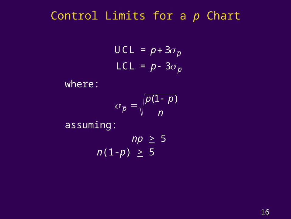
Control Limits for a p Chart

where:

assuming: np > 5 n(1-p) > 5

UCL = p p 3

LCL = p p 3

pp p

n

( )1

17 17 Slide

Slide

Control Limits for an np Chart

assuming: np > 5 n(1-p) > 5

Note: If computed LCL is negative, set LCL = 0

UCL = np np p 3 1( )

LCL = np np p 3 1( )

18 18 Slide

Slide

Acceptance Sampling

Acceptance sampling is a statistical method that enables us to base the accept-reject decision on the inspection of a sample of items from the lot.

Acceptance sampling has advantages over 100% inspection including: less expensive, less product damage, fewer people involved, . . . and more.

19 19 Slide

Slide

Acceptance Sampling Procedure

Lot received

Sample selected

Sampled itemsinspected for quality

Results compared withspecified quality characteristics

Accept the lot Reject the lot

Send to productionor customer

Decide on dispositionof the lot

Quality is not satisfactory

Quality issatisfactory

20 20 Slide

Slide

Acceptance Sampling

Acceptance sampling is based on hypothesis-testing methodology.

The hypothesis are: H0: Good-quality lot

Ha: Poor-quality lot

21 21 Slide

Slide

The Outcomes of Acceptance Sampling

Type I and Type II Errors State of the Lot

H0 True Ha True

Decision Good-Quality Lot Poor-Quality Lot

Accept H0 Correct Type II Error

Accept the Lot Decision Consumer’s Risk

Reject H0 Type I Error Correct

Reject the Lot Producer’s Risk Decision

22 22 Slide

Slide

Probability of Accepting a Lot

Binomial Probability Function for Acceptance Sampling

where:n = sample sizep = proportion of defective items in lotx = number of defective items in sample

f(x) = probability of x defective items in sample

f xn

x n xp px n x( )

!!( )!

( )( )

1

23 23 Slide

Slide

Example: Acceptance Sampling

An inspector takes a sample of 20 items from a lot.

Her policy is to accept a lot if no more than 2 defective

items are found in the sample.Assuming that 5 percent of a lot is defective, what is

the probability that she will accept a lot? Reject a lot?

n = 20, c = 2, and p = .05 P(Accept Lot) = f(0) + f(1) + f(2)

= .3585 + .3774 + .1887

= .9246 P(Reject Lot) = 1 - .9246 = .0754

24 24 Slide

Slide

Example: Acceptance Sampling

Using the Tables of Binomial Probabilities

pn x .05 .10 .15 .20 .25 .30 .35 .40 .45 .5020 0 .3585 .1216 .0388 .0115 .0032 .0008 .0002 .0000 .0000 .0000

1 .3774 .2702 .1368 .0576 .0211 .0068 .0020 .0005 .0001 .00002 .1887 .2852 .2293 .1369 .0669 .0278 .0100 .0031 .0008 .00023 .0596 .1901 .2428 .2054 .1339 .0716 .0323 .0123 .0040 .00114 .0133 .0898 .1821 .2182 .1897 .1304 .0738 .0350 .0139 .00465 .0022 .0319 .1028 .1746 .2023 .1789 .1272 .0746 .0365 .01486 .0003 .0089 .0454 .1091 .1686 .1916 .1712 .1244 .0746 .03707 .0000 .0020 .0160 .0545 .1124 .1643 .1844 .1659 .1221 .07398 .0000 .0004 .0046 .0222 .0609 .1144 .1614 .1797 .1623 .12019 .0000 .0001 .0011 .0074 .0271 .0654 .1158 .1597 .1771 .1602

25 25 Slide

Slide

Operating Characteristic Curve

.10.10

.20.20

.30.30

.40.40

.50.50

.60.60

.70.70

.80.80

.90.90

Pro

bab

ilit

y o

f A

ccep

tin

g t

he L

ot

Pro

bab

ilit

y o

f A

ccep

tin

g t

he L

ot

0 5 10 15 20 25 0 5 10 15 20 25

1.001.00

Percent Defective in the Lotp0

p1

b

(1 - a)

an = 15, c = 0

p0 = .03, p1 = .15

a = .3667, b = .0874

26 26 Slide

Slide

Multiple Sampling Plans

A multiple sampling plan uses two or more stages of sampling.

At each stage the decision possibilities are:• stop sampling and accept the lot,• stop sampling and reject the lot, or• continue sampling.

Multiple sampling plans often result in a smaller total sample size than single-sample plans with the same Type I error and Type II error probabilities.

27 27 Slide

Slide

A Two-Stage Acceptance Sampling Plan

Inspect n1 items

Find x1 defective items in this sample

Is x1 < c1 ?

Is x1 > c2 ?

Inspect n2 additional items

Acceptthe lot

Rejectthe lot

Is x1 + x2 < c3 ?

Find x2 defective items in this sample

Yes

YesNo

No

NoYes

28 28 Slide

Slide

The End of Chapter 13