1 4. advanced chemical thermodynamics. 4.0 colligative properties vapor pressure lowering:...
TRANSCRIPT
1
4. Advanced chemical thermodynamics
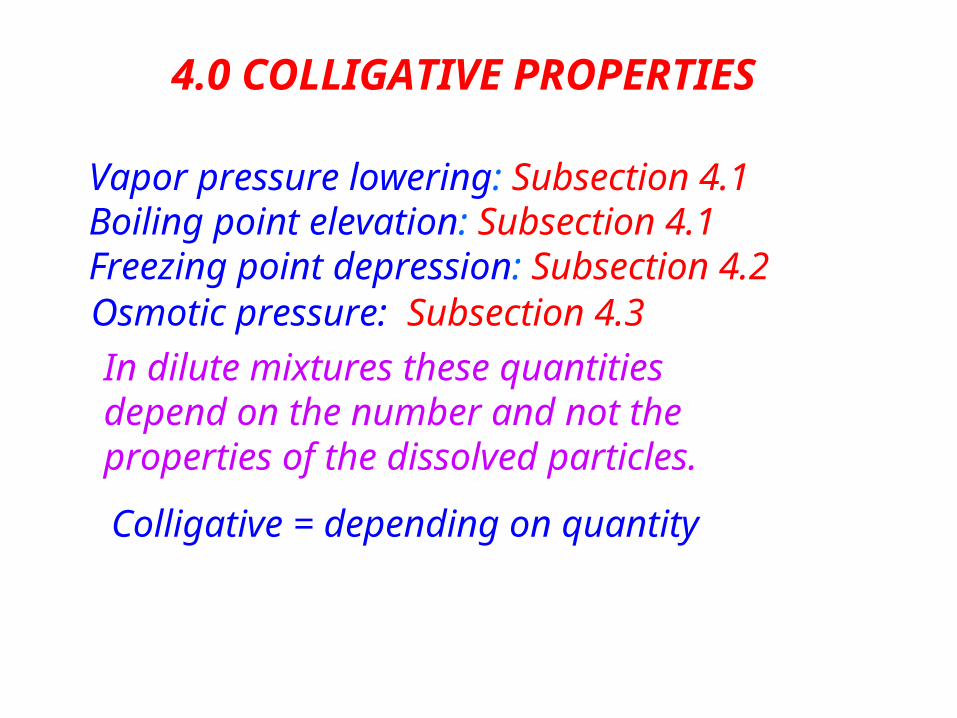
4.0 COLLIGATIVE PROPERTIES
Vapor pressure lowering: Subsection 4.1Boiling point elevation: Subsection 4.1Freezing point depression: Subsection 4.2 Osmotic pressure: Subsection 4.3
In dilute mixtures these quantities depend on the number and not the properties of the dissolved particles.
Colligative = depending on quantity
3
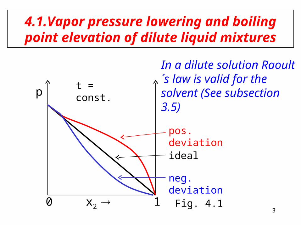
4.1.Vapor pressure lowering and boiling point elevation of dilute liquid mixtures
0
p
x2 1
t = const.
In a dilute solution Raoult´s law is valid for the solvent (See subsection 3.5)
pos. deviation
ideal
neg. deviation
Fig. 4.1
4
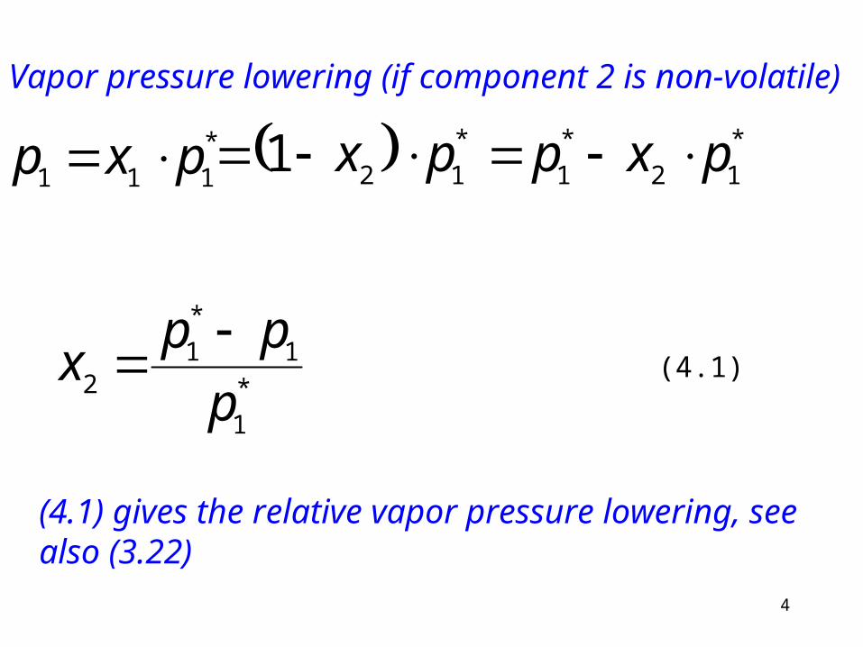
Vapor pressure lowering (if component 2 is non-volatile)
*
111 pxp *
121 px *
12
*
1 pxp
*
1
1
*
12 p
ppx
(4.1) gives the relative vapor pressure lowering, see also (3.22)
(4.1)
5
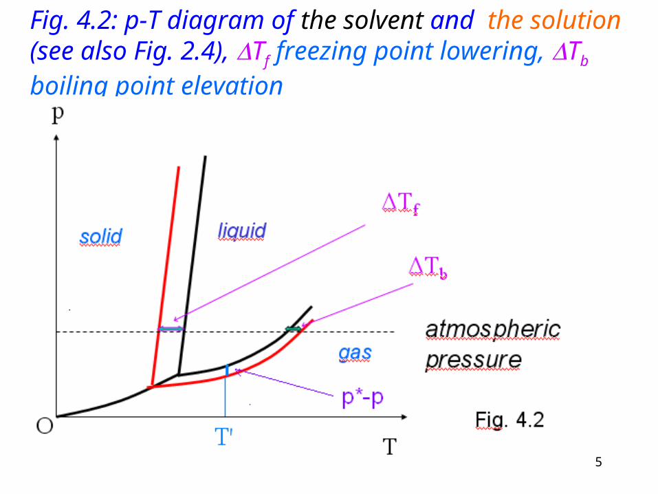
Fig. 4.2: p-T diagram of the solvent and the solution (see also Fig. 2.4), Tf freezing point lowering, Tb
boiling point elevation

6
Have a look on Fig. 4.2! There are compared the solvent (black curve) and the solution (red curve) properties in a p-T diagram.
The vapor pressure decreases in comparison of the p-T diagrams of the solvent and the solution. At a constant T’ temperature the p*-p is observable.
The boiling point increases (Tb). On the figure you can see it at atmospheric pressure.
In contrary to the behavor of the boiling point the freezing point decreases as effect of the solving (Tf).
7
1
*
1
*
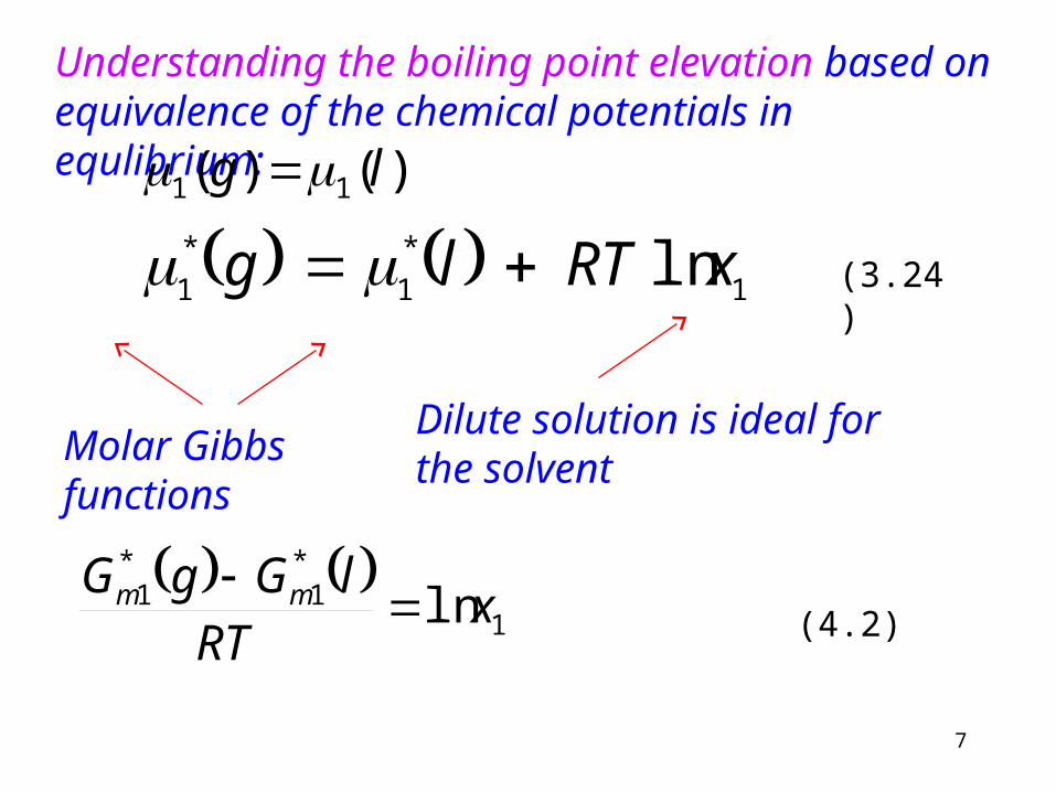
1 ln xRTlg
Molar Gibbs functions
Dilute solution is ideal for the solvent
1
*1
*1 ln x
RT
lGgG mm
Understanding the boiling point elevation based on equivalence of the chemical potentials in equlibrium:
)()( 11 lg
(3.24)
(4.2)
8
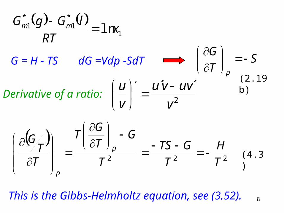
G = H - TS dG =Vdp -SdT ST
G
p
Derivative of a ratio:2
,´´
v
uvvu
v
u
222 T
H
T
GTS
T
GT
GT
TT
Gp
p
This is the Gibbs-Helmholtz equation, see (3.52).
1
*1
*1 ln x
RTlGgG mm
(2.19b)
(4.3)
9
dT
xdRT
lGgGT
mm 1*
1*
1 ln
dT
xdRT
gHlH mm 12
*1
*1 ln
211 )(ln
RTvapH
dTxd m (molar heat of
vaporization)
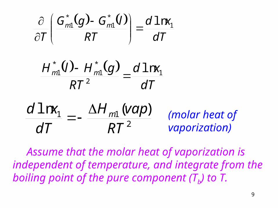
Assume that the molar heat of vaporization is independent of temperature, and integrate from the boiling point of the pure component (Tb) to T.

10
b
m
TTRvapH
x11)(
ln 11
Substitute the mole fraction of the solute: x1 = 1-x2
Take the power series of ln(1-x2), and ignore the higher terms since they are negligible (x2<<1)
...32
)1ln(ln3
2
2
2221
xxxxx
(4.4)
11
b
m
TTRvapH
x11)(1
2
2b
1m
b
b1m2 T
T
R
)vap(H
TT
TT
R
)vap(Hx
21
2
)(x
vapHRT
Tm
b
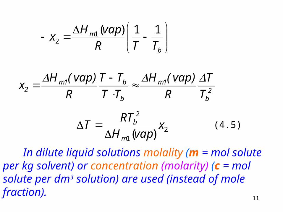
In dilute liquid solutions molality (m = mol solute per kg solvent) or concentration (molarity) (c = mol solute per dm3 solution) are used (instead of mole fraction).
(4.5)

12
1212
1
2
21
22 Mm
solventofmassMn
nn
nnn
x
m2: molality of soluteM1: molar mass of solvent
2
1
1
2
)(m
vapH
MRTT
m
b
Includes the parameters of the solvent only: Kb
2mKT b
Kb: molal boiling point elevation
With this
(4.6)
(4.7)
13
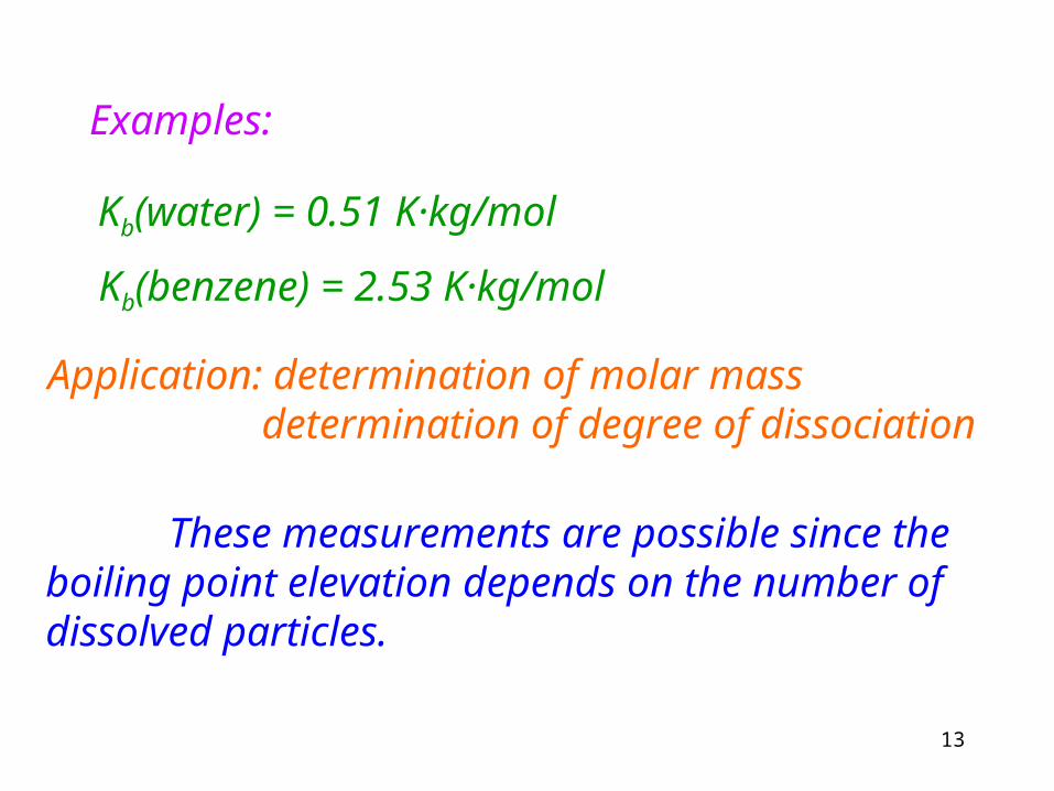
Kb(water) = 0.51 K·kg/mol
Kb(benzene) = 2.53 K·kg/mol
Application: determination of molar mass determination of degree of dissociation
These measurements are possible since the boiling point elevation depends on the number of dissolved particles.
Examples:
14
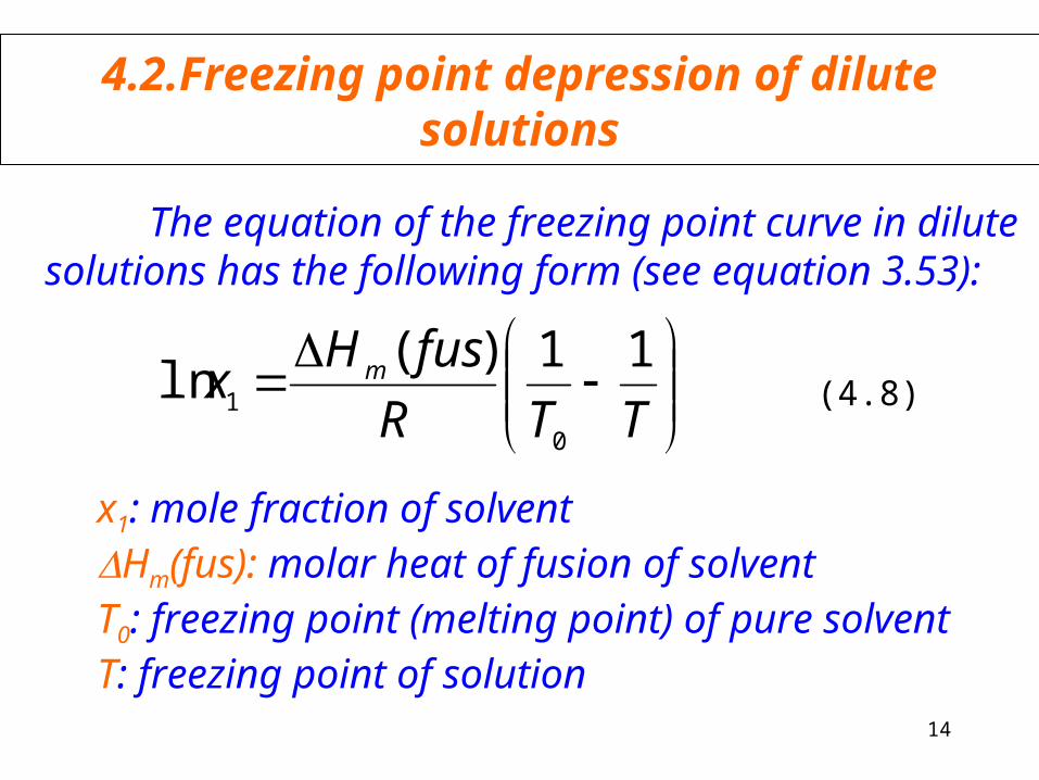
4.2.Freezing point depression of dilute solutions
TTR
fusHx m 11)(
ln0
1
The equation of the freezing point curve in dilute solutions has the following form (see equation 3.53):
x1: mole fraction of solventHm(fus): molar heat of fusion of solvent T0: freezing point (melting point) of pure solventT: freezing point of solution
(4.8)
15
221 x)x1ln(xln
0
0
02
)(11)(TTTT
RfusH
TTRfusH
x mm
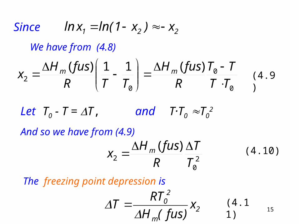
Let T0 - T = T, and T·T0 T02
20
2
)(T
TR
fusHx m
2m
20 x
)fus(H
RTT
Since
We have from (4.8)
(4.9)
And so we have from (4.9)
(4.10)
The freezing point depression is
(4.11)

16
Since x2 m2M1, we have
21
20
)(m
fusHMRT
Tm
2mKT f Kf is molal freezing point depression
Kf(water) = 1.83 K·kg/mol
Kf(benzene) = 5.12 K·kg/mol
Kf(camphor) = 40 K·kg/mol
(4.12)
This multipier (Kf) contains solvent parameters only,
(4.13)
The following examples are given in molality units
Molality unit: moles solute pro 1 kg solvent
17
Osmosis: two solutions of the same substance with different concentrations are separated by a semi-permeable membrane (a membrane permeable for the solvent but not for the solute). Then the solvent starts to go through the membrane from the more dilute solution towards the more concentrated solution.
Why ?
Because the chemical potential of the solvent is greater in the more dilute solution.
The „more dilute” solution may be a pure solvent, component 1.
4.3. Osmotic pressure

18
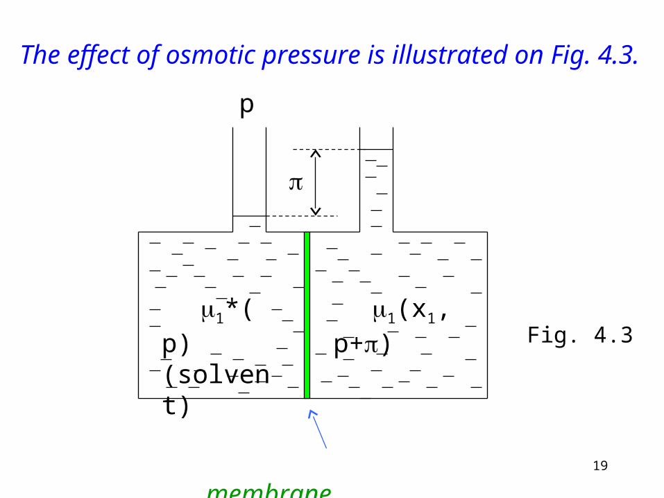
If the more concentrated solution cannot expand freely, its pressure increases, increasing the chemical potential. Sooner or later an equilibrium is attained. (The chemical potential of the solvent is equal in the two solutions.)
The measured pressure difference between the two sides of the semipermeable membrane is called osmotic pressure ().
What does osmotic pressure depend on?
van´t Hoff found (1885) for dilute solutions (solute:component 2) V = n2RT
= c2RT(4.14) is similar to the ideal gas law, see equ. (1.27)
(4.14)
(4.15)
19
1*(p) (solvent)
p
1(x1,p+)
membrane
The effect of osmotic pressure is illustrated on Fig. 4.3.
Fig. 4.3
20
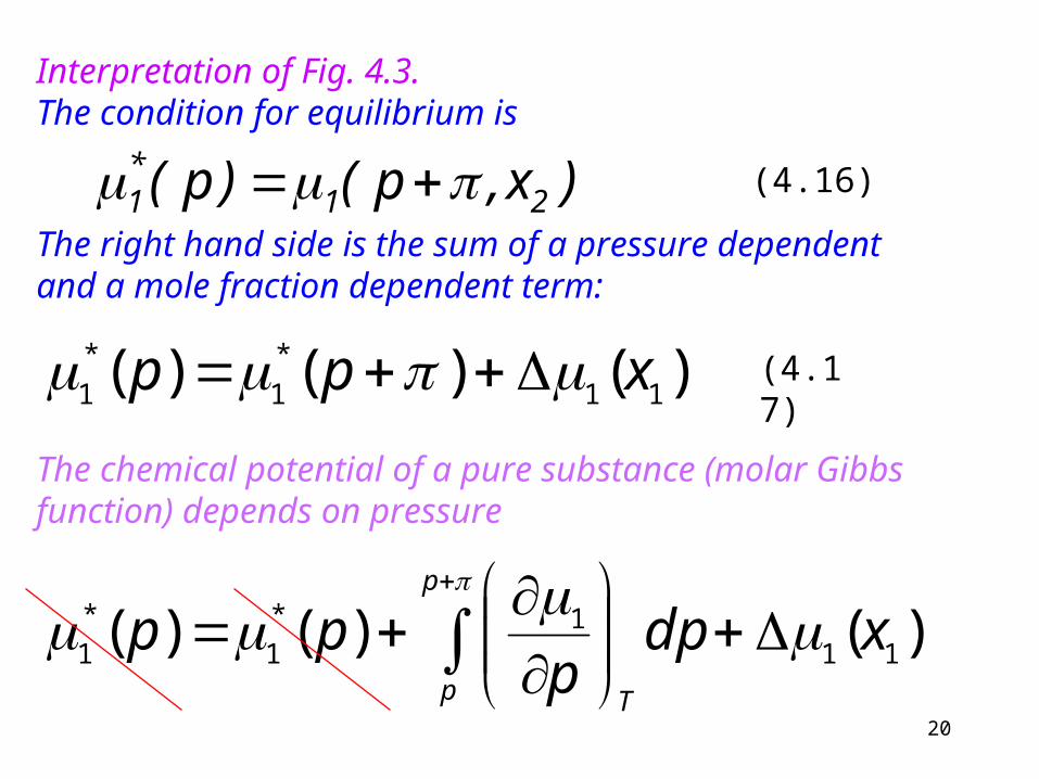
Interpretation of Fig. 4.3.The condition for equilibrium is
)x,p()p( 21*1
The right hand side is the sum of a pressure dependent and a mole fraction dependent term:
)()()( 11
*
1
*
1 xpp
The chemical potential of a pure substance (molar Gibbs function) depends on pressure
)()()( 111*
1
*
1 xdpp
ppp
p T
(4.16)
(4.17)

21
Vp
G
T
V1 is the partial molar volume (see equ. 3.5). Its pressure dependence can be neglected. (The volume of a liquid only slightly changes with pressure), so the integral is only V1. So we have
For 1
T
1 Vp
0 = V1 +1(x1)
1(x1) = -V1
This equation is good both for ideal and for real solutions. Measuring the osmotic pressure we can determine (and the activity).
see (2.19b)
Rearranged (4.18)
22
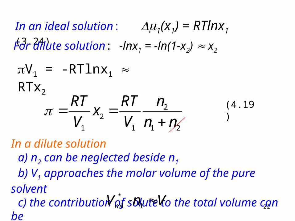
In an ideal solution: 1(x1) = RTlnx1 (3.24)
For dilute solution: -lnx1 = -ln(1-x2) x2
V1 = -RTlnx1 RTx2
21
2
1
2
1 nn
n
V
RTx
V
RT
In a dilute solution a) n2 can be neglected beside n1 b) V1 approaches the molar volume of the pure solvent c) the contribution of solute to the total volume can be neglected ( ). VnVm 1
*
1
(4.19)
23
2nV
RT
RTnV 2
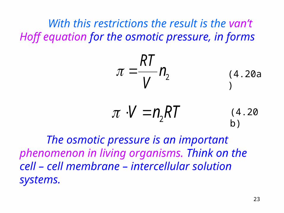
With this restrictions the result is the van’t Hoff equation for the osmotic pressure, in forms
(4.20a)
(4.20b)
The osmotic pressure is an important phenomenon in living organisms. Think on the cell – cell membrane – intercellular solution systems.
24
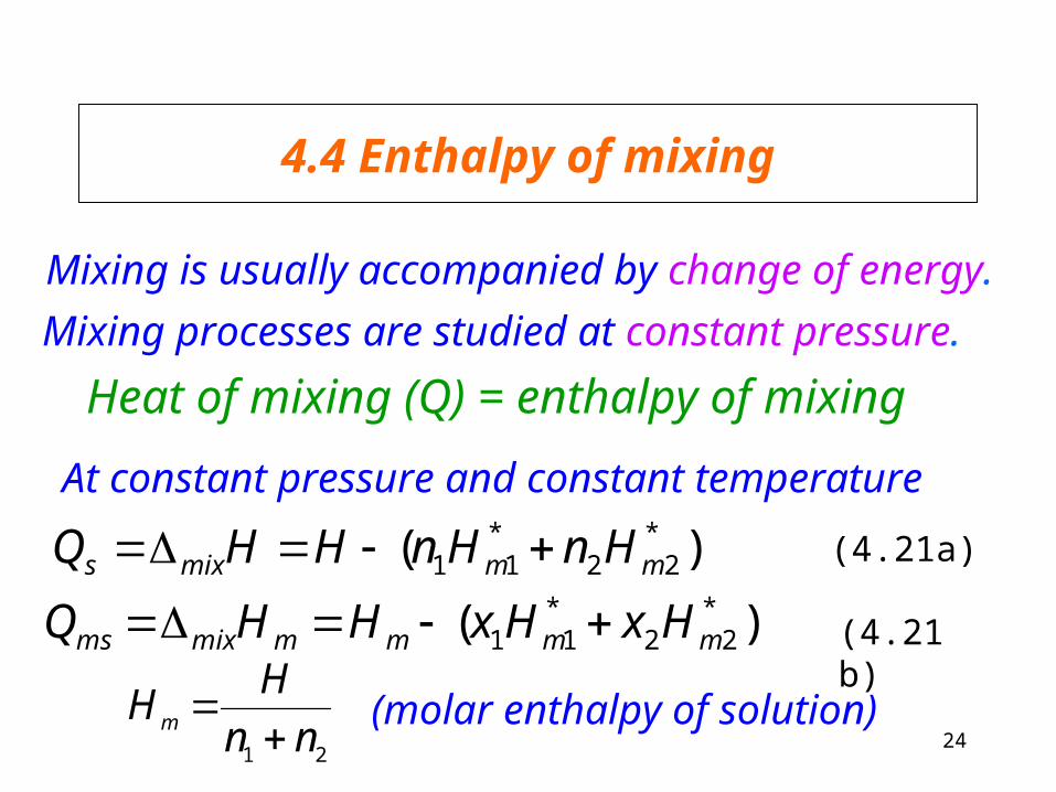
4.4 Enthalpy of mixing
Mixing is usually accompanied by change of energy.
Heat of mixing (Q) = enthalpy of mixing
Mixing processes are studied at constant pressure.
)( *22
*11 mmmixs HnHnHHQ
)( *22
*11 mmmmmixms HxHxHHQ
21 nn
HHm
(molar enthalpy of solution)
At constant pressure and constant temperature
(4.21a)
(4.21b)
25
Molar heat of mixing (called also integral heat of solution, and molar enthalpy of mixing)
is the enthalpy change when 1 mol solution is produced from the components
at constant temperature and pressure.
In case of ideal solutions the enthalpy is additive, Qms= 0, if there is no change of state.
In real solutions Qms (molar heat of fusion) is not zero. The next figures present the deviations from the ideal behavior.
26
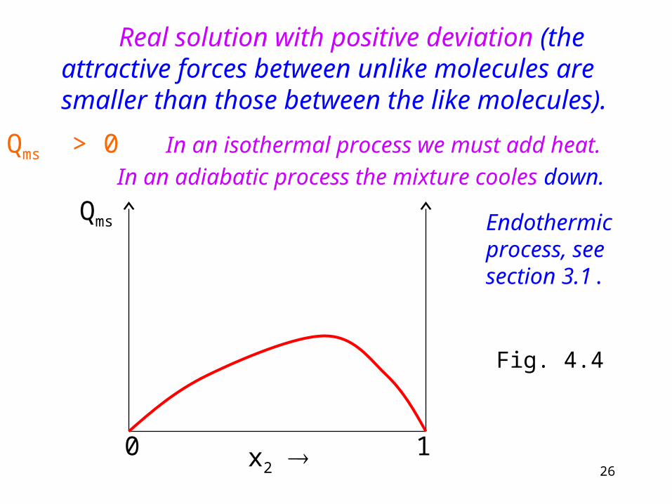
Real solution with positive deviation (the attractive forces between unlike molecules are smaller than those between the like molecules).
Qms > 0 In an isothermal process we must add heat.
In an adiabatic process the mixture cooles down.
x2 0 1
Qms Endothermic process, see section 3.1.
Fig. 4.4

27
Real solution with negative deviation (the attractive forces between unlike molecules are greater than those between the like molecules).
Qms < 0 In an isothermal process we must distract heat. In an adiabatic process the mixture warmes up.
x2 0 1
Qms
Exothermic process, see section 3.1.
Fig. 4.5.
28
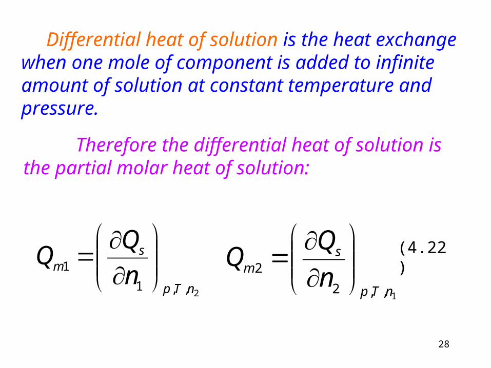
Differential heat of solution is the heat exchange when one mole of component is added to infinite amount of solution at constant temperature and pressure.
2,,1
1
nTp
sm n
1,,2
2
nTp
sm n
Therefore the differential heat of solution is the partial molar heat of solution:
(4.22)
29x2
0 1
Qms
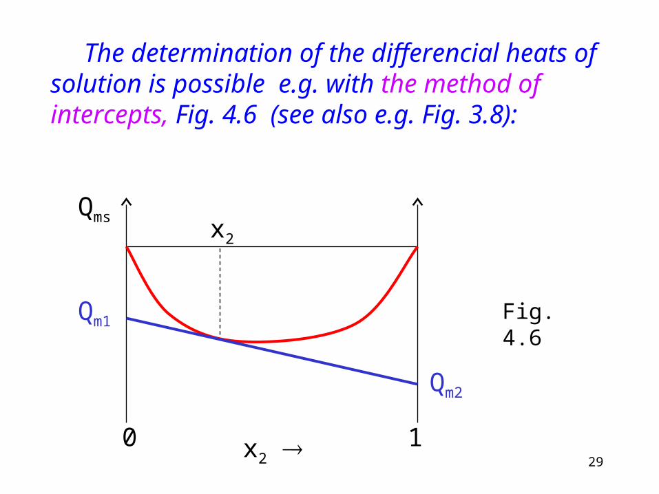
The determination of the differencial heats of solution is possible e.g. with the method of intercepts, Fig. 4.6 (see also e.g. Fig. 3.8):
x2
Qm1
Qm2
Fig. 4.6
30
)( *
22
*
11 mms HnHnHQ
)( *
22
*
11
1,,1
1
2
mm
nTp
m HnHnnn
HQ
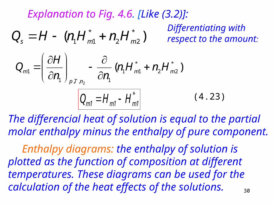
*1m1m1m HHQ
The differencial heat of solution is equal to the partial molar enthalpy minus the enthalpy of pure component.
Enthalpy diagrams: the enthalpy of solution is plotted as the function of composition at different temperatures. These diagrams can be used for the calculation of the heat effects of the solutions.
Explanation to Fig. 4.6. [Like (3.2)]:Differentiating with respect to the amount:
(4.23)
31
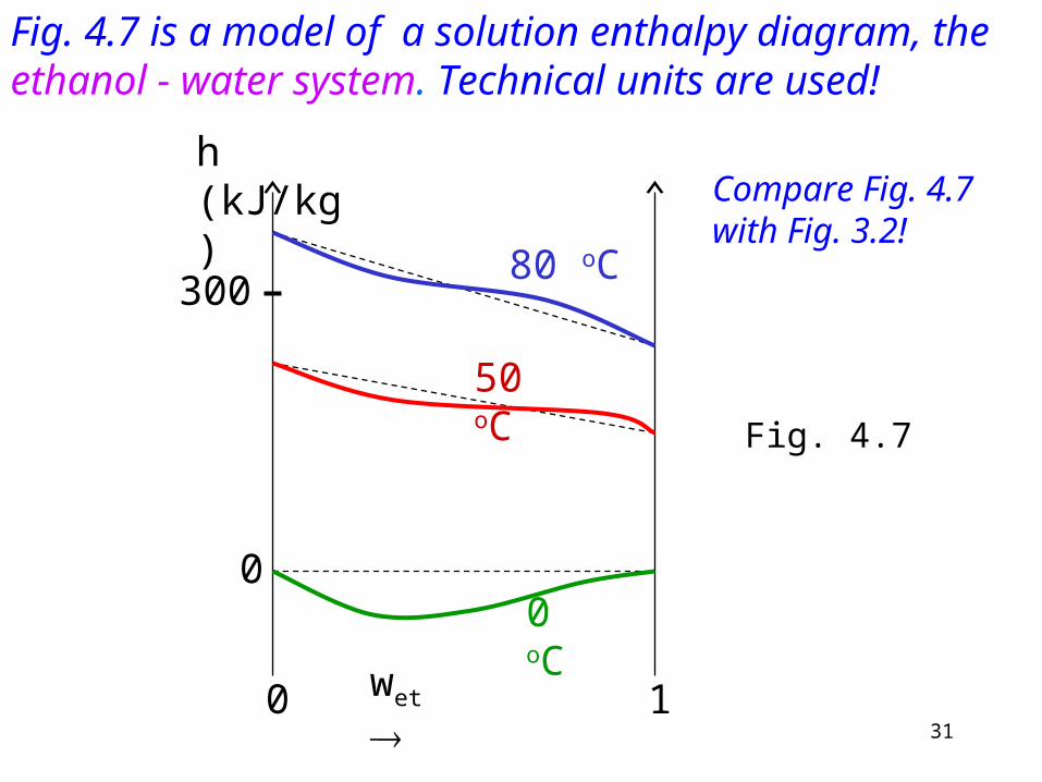
Fig. 4.7 is a model of a solution enthalpy diagram, the ethanol - water system. Technical units are used!
wet
h (kJ/kg)
300
00 oC
50 oC
80 oC
0 1
Fig. 4.7
Compare Fig. 4.7 with Fig. 3.2!
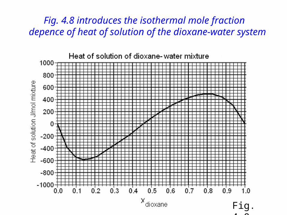
Fig. 4.8 introduces the isothermal mole fraction depence of heat of solution of the dioxane-water system
Fig. 4.8
33
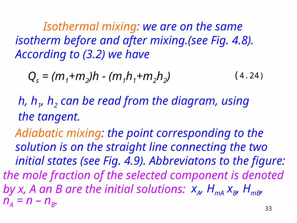
Isothermal mixing: we are on the same isotherm before and after mixing.(see Fig. 4.8). According to (3.2) we have
Qs = (m1+m2)h - (m1h1+m2h2)
h, h1, h2 can be read from the diagram, using the tangent.
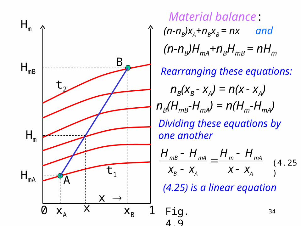
Adiabatic mixing: the point corresponding to the solution is on the straight line connecting the two initial states (see Fig. 4.9). Abbreviatons to the figure:
the mole fraction of the selected component is denoted by x, A an B are the initial solutions: xA, HmA xB, HmB, nA = n – nB.
(4.24)
34
Hm
x 10
A
B
xBxA
HmA
HmB
t1
t2
Material balance:(n-nB)xA+nBxB = nx and
(n-nB)HmA+nBHmB = nHm
nB(HmB-HmA) = n(Hm-HmA)
nB(xB - xA) = n(x - xA)
A
mAm
AB
mAmB
xx
HH
xx
HH
(4.25) is a linear equation
Hm
x Fig. 4.9
(4.25)
Rearranging these equations:
Dividing these equations by one another
35
A
AB
mAmBmAm xx
xx
HHHH
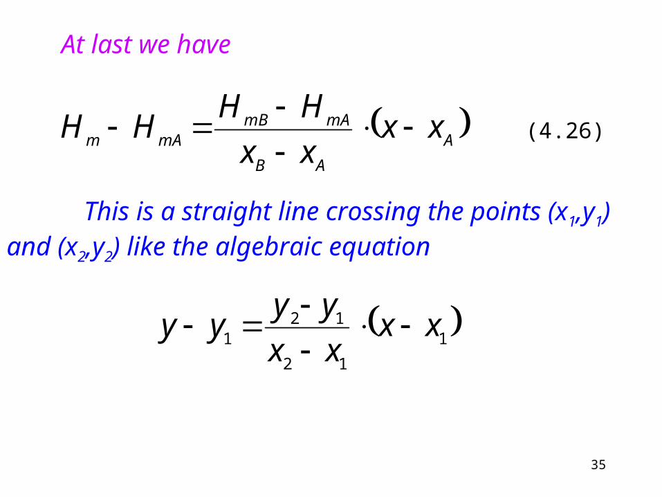
This is a straight line crossing the points (x1,y1) and (x2,y2) like the algebraic equation
1
12
121 xx
xx
yyyy
At last we have
(4.26)
36
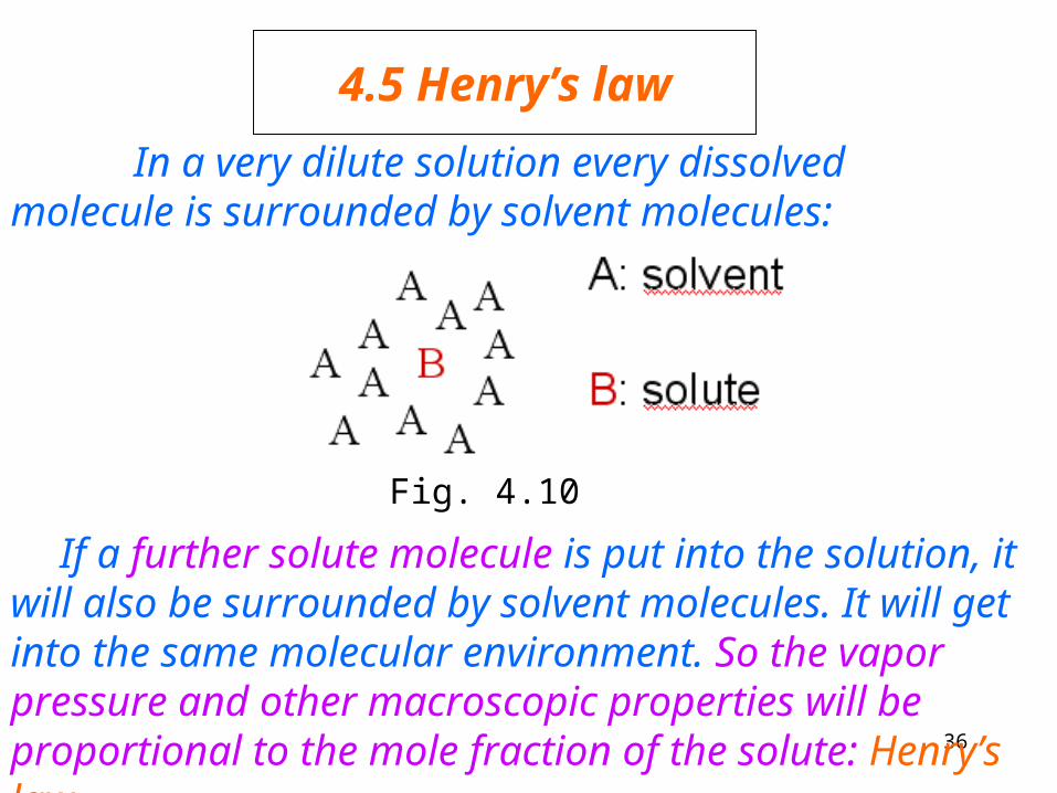
4.5 Henry’s law
In a very dilute solution every dissolved molecule is surrounded by solvent molecules:
If a further solute molecule is put into the solution, it will also be surrounded by solvent molecules. It will get into the same molecular environment. So the vapor pressure and other macroscopic properties will be proportional to the mole fraction of the solute: Henry’s law.
Fig. 4.10
37
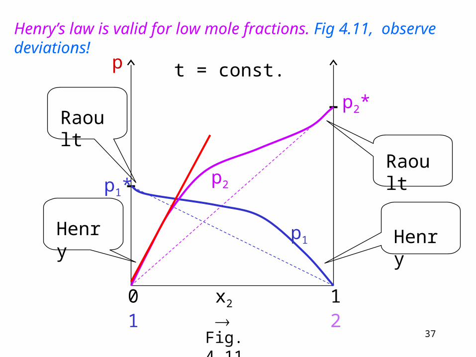
Henry’s law is valid for low mole fractions. Fig 4.11, observe deviations!
x2 0 11 2
p1*
p2*
t = const.p
p1
p2
Henry
Raoult
Raoult
Henry
Fig. 4.11

38
Where component 2 is the solute, the left hand side of Fig. 4.11):
22 xkp H kH is the Henry constant
In the same range the Raoult´s law applies to the solvent:
1*11 xpp
The two equations are similar. There is a difference in the constants. p1* has an exact physical meaning (the vapor pressure of pure substance) while kH does not have any exact meaning. In a dilute solution the Raoult´s law is valid for the solvent and Henry´s law is valid for the solute.
(4.27)
like (3.18)

39
4.6 Solubility of gases
The solution of gases in liquids are generally dilute, so we can use Henry´s law.
The partial pressure of the gas above the solution is proportional to the mole fraction in the liquid phase.
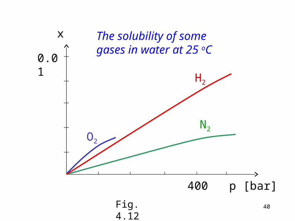
Usually the mole fraction (or other parameter expressing the composition) is plotted against the pressure. If Henry´s law applies, this function is a straight line. See e.g. the solubilty of some gases on Fig. 4.12!
40
0.01
O2
400 p [bar]
x
H2
N2
The solubility of some gases in water at 25 oC
Fig. 4.12
41
In case of N2 and H2 the function is linear up to several hundred bars (Henry´s law applies), in case of O2 the function is not linear even below 100 bar.
Temperature dependence of solubility of gases
Le Chatelier´s principle: a system in equilibrium, when subjected to a perturbation, responds in a way that tends to minimize its effect.
Solution of a gas is a change of state: gas liquid. It is usually an exothermic process. Increase of temperature: the equilibrium is shifted towards the endothermic direction desorption. The solubility of gases usually decreases with increasing the temperature.
Absorption - desorption

42
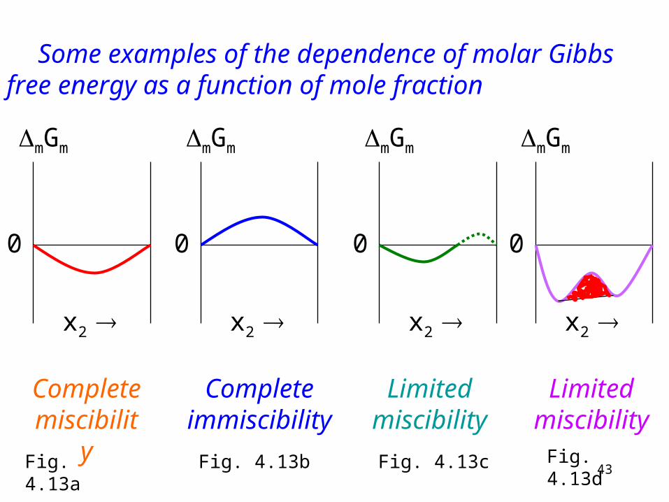
4.7 Thermodynamic stability of solutions
One requirement for the stability is the negative Gibbs function of mixing.
The negative Gibbs function of mixing does not necessary mean solubility (see Fig. 4.13d diagram of the next figure).
Other requirement: The second derivative of the Gibbs free energy of mixing with respect to composition must be positive.
43
0
mGm
x2
0
mGm
x2
0
mGm
x2
0
mGm
x2
Complete miscibility
Complete immiscibility
Limited miscibility
Limited miscibility
Some examples of the dependence of molar Gibbs free energy as a function of mole fraction
Fig. 4.13a Fig. 4.13b Fig. 4.13c Fig. 4.13d
44
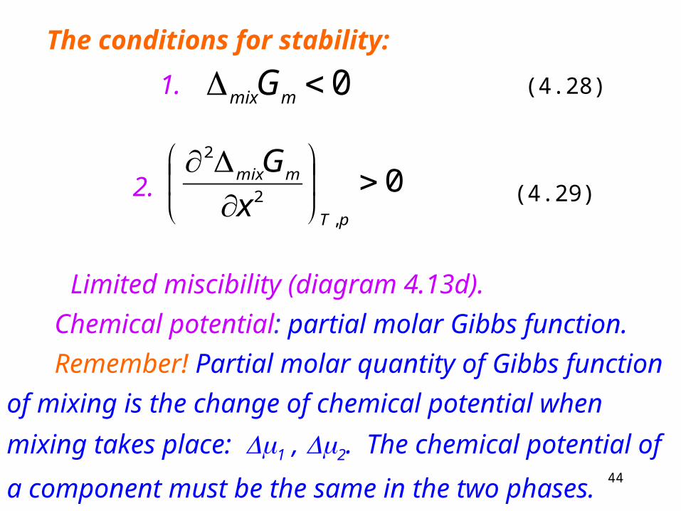
The conditions for stability:
0 mmixG1.
0,
2
2
pT
mmix
x
G2.
Limited miscibility (diagram 4.13d).
Chemical potential: partial molar Gibbs function.
Remember! Partial molar quantity of Gibbs function of
mixing is the change of chemical potential when mixing
takes place: 1 , 2. The chemical potential of a
component must be the same in the two phases.
(4.28)
(4.29)
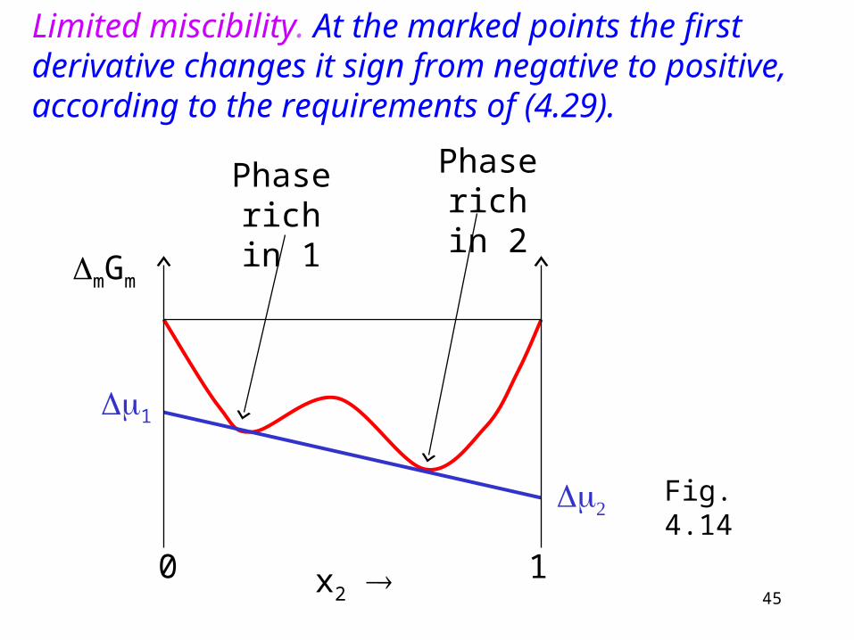
45x2
0 1
mGm
1
Phase rich in 1
Phase rich in 2
Limited miscibility. At the marked points the first derivative changes it sign from negative to positive, according to the requirements of (4.29).
Fig. 4.14
46
The common tangent of the two curves produces and (method of intercepts). Fig. 4.14.
1 must be the same in the phase rich in 1 as in the phase rich in 2 according to ther requirement of equilibrium. The same applies to .

47
4.8. Liquid - liquid phase equilibria
The mutual solubility depends on temperature. In most cases the solubility increases with increasing temperature.
n-hexane nitrobenzene
0
t [oC]
201 phase
2phases
tuc
tuc : upper critical solution temperature
u: upperIn this case the formed complex decomposes at higher temperatures.
Fig. 4.15
48
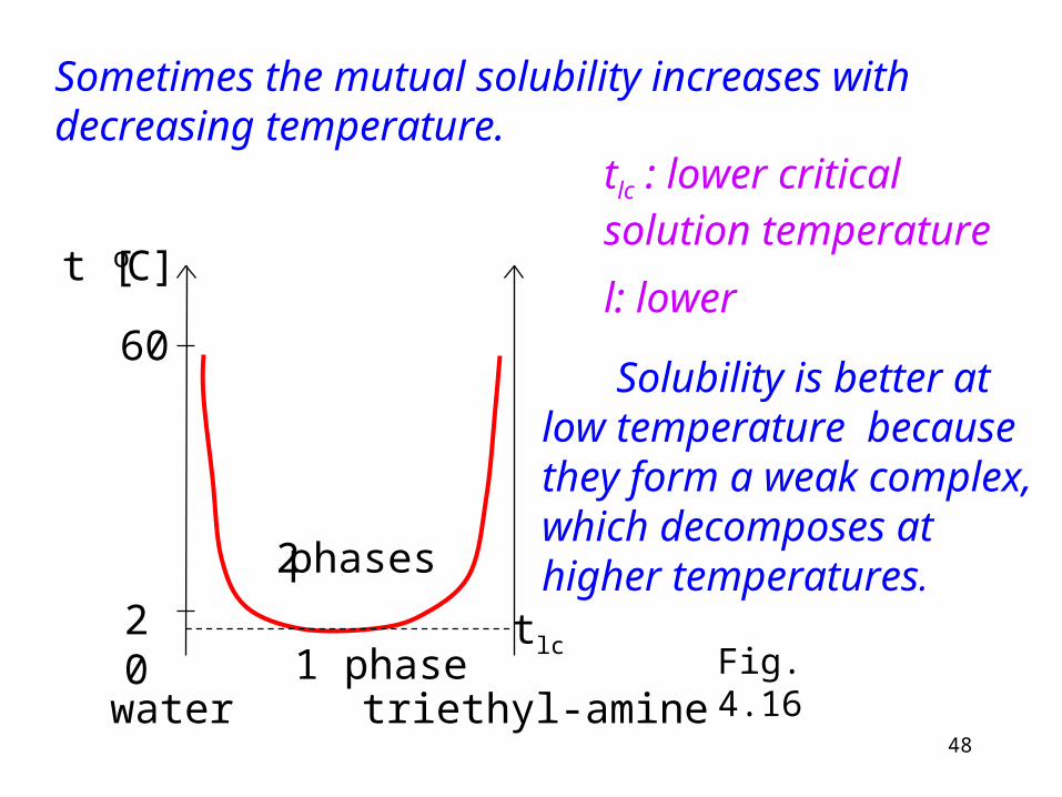
Sometimes the mutual solubility increases with decreasing temperature.
water triethyl-amine
20
t [oC]
60
1 phase
2 phases
tlc
tlc : lower critical solution temperature
l: lower
Solubility is better at low temperature because they form a weak complex, which decomposes at higher temperatures.
Fig. 4.16

49
In a special case there are both upper and lower critical solution temperatures.
Low t: weak complexesHigher t: they decompose
At even higher temperatures the thermal motion homogenizes the system.
water nicotine
60
t [oC]
200
2 phases
1 phase
tlc
tuc
1 phase
x
Fig, 4.17
50
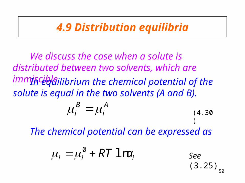
4.9 Distribution equilibria
We discuss the case when a solute is distributed between two solvents, which are immiscible.
In equilibrium the chemical potential of the solute is equal in the two solvents (A and B).
Ai
Bi
The chemical potential can be expressed as
iii aRT ln0
(4.30)
See (3.25)
51
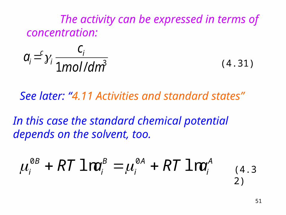
The activity can be expressed in terms of concentration:
3/1 dmmol
ca i
ic
i
See later: “4.11 Activities and standard states”
In this case the standard chemical potential depends on the solvent, too.
A
i
A
i
B
i
B
i aRTaRT lnln 00
(4.31)
(4.32)

52
RTaa
B
i
A
iA
i
B
i
00
lnln
RTa
a B
i
A
i
A
i
B
i
00
ln
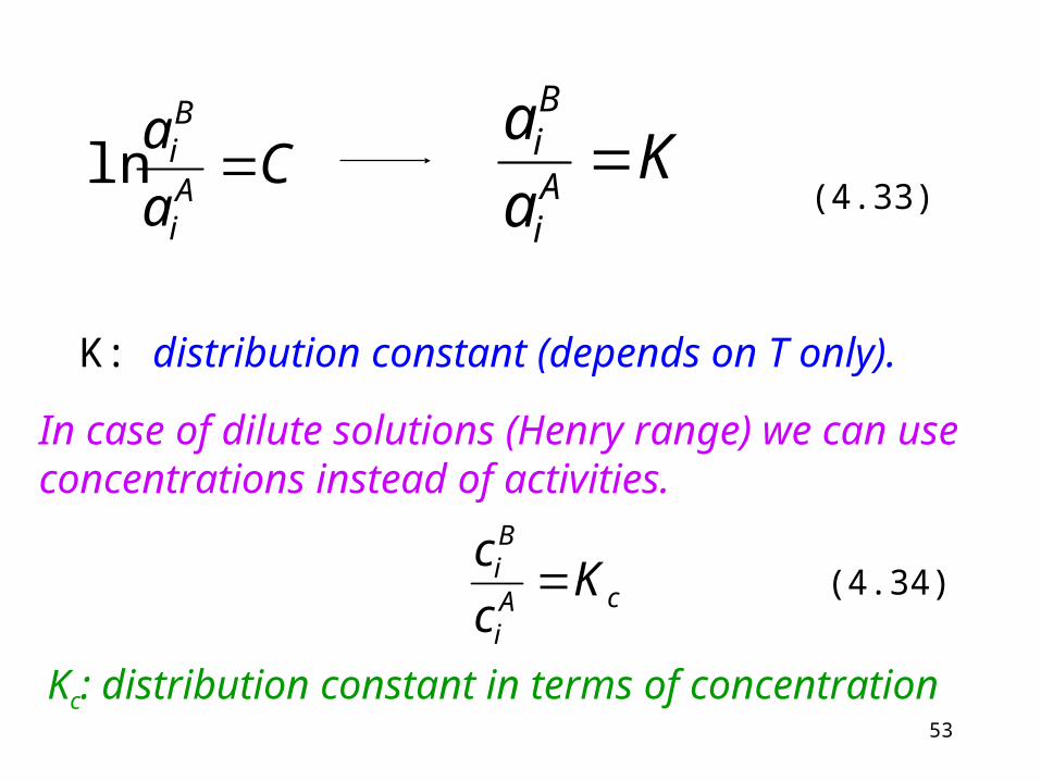
The quantities on the right hand side depend on temperature only (i.e. they do not depend on composition).
53
K: distribution constant (depends on T only).
In case of dilute solutions (Henry range) we can use concentrations instead of activities.
Kc: distribution constant in terms of concentration
Ca
aAi
Bi ln K
a
aAi
Bi
cAi
Bi K
c
c
(4.33)
(4.34)

54
Processes based on distribution are called extraction.
Calculation of the efficiency of extraction in a lab
V´ V
C0 C1
0 C1’
We assume that the solutions are dilute and their volume does not change during extraction. (The two solvents do not dissolve each other at all: Fig. 4.18).
Fig. 4.18
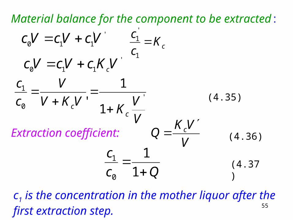
55
Material balance for the component to be extracted:''
110 VcVcVc '
110 VKcVcVc c
c1 is the concentration in the mother liquor after the first extraction step.
cKc
c
1
'1
VV
KVKV
V
c
c
cc
'0
1
1
1
'
V
VKQ c
Qc
c
1
1
0
1
Extraction coefficient:
(4.35)
(4.36)
(4.37)
56
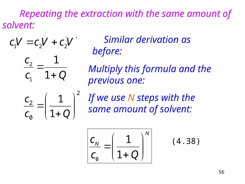
Repeating the extraction with the same amount of solvent:
''
221 VcVcVc Similar derivation as before:
Qc
c
1
1
1
2Multiply this formula and the previous one:
2
0
2
1
1
Qc
c If we use N steps with the same amount of solvent:
N
N
Qc
c
1
1
0
(4.38)
57
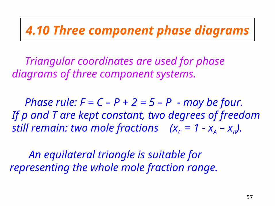
4.10 Three component phase diagrams
Triangular coordinates are used for phase diagrams of three component systems.
Phase rule: F = C – P + 2 = 5 – P - may be four.If p and T are kept constant, two degrees of freedom still remain: two mole fractions (xC = 1 - xA – xB).
An equilateral triangle is suitable for representing the whole mole fraction range.

58
A B
C
Each composition corresponds to one point.
E.g. xA = 0.2, xB = 0.5
xA
0.2
xB 0.5
The point representing the composition is the crossing point of the two lines
xC
We draw a parallel line with the line opposite the apex of the substance.
Fig. 4.19
59
A B
C
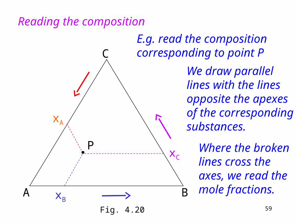
Reading the composition
xA
xB
Where the broken lines cross the axes, we read the mole fractions.
xC
We draw parallel lines with the lines opposite the apexes of the corresponding substances.
P
E.g. read the composition corresponding to point P
Fig. 4.20
60
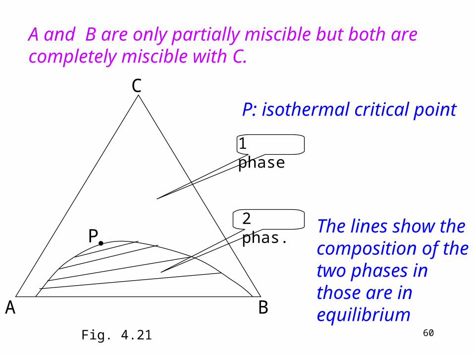
A B
C
P
1 phase
2 phas.
A and B are only partially miscible but both are completely miscible with C.
The lines show the composition of the two phases in those are in equilibrium
P: isothermal critical point
Fig. 4.21
61
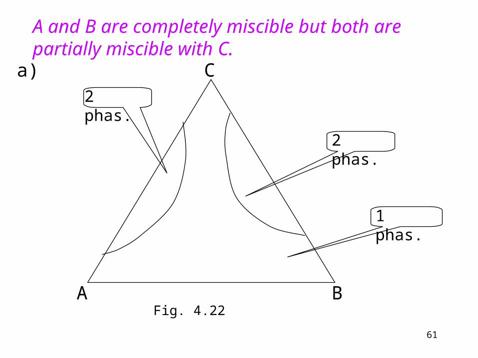
A B
C
1 phas.
2 phas.
2 phas.
a)
A and B are completely miscible but both are partially miscible with C.
Fig. 4.22
62
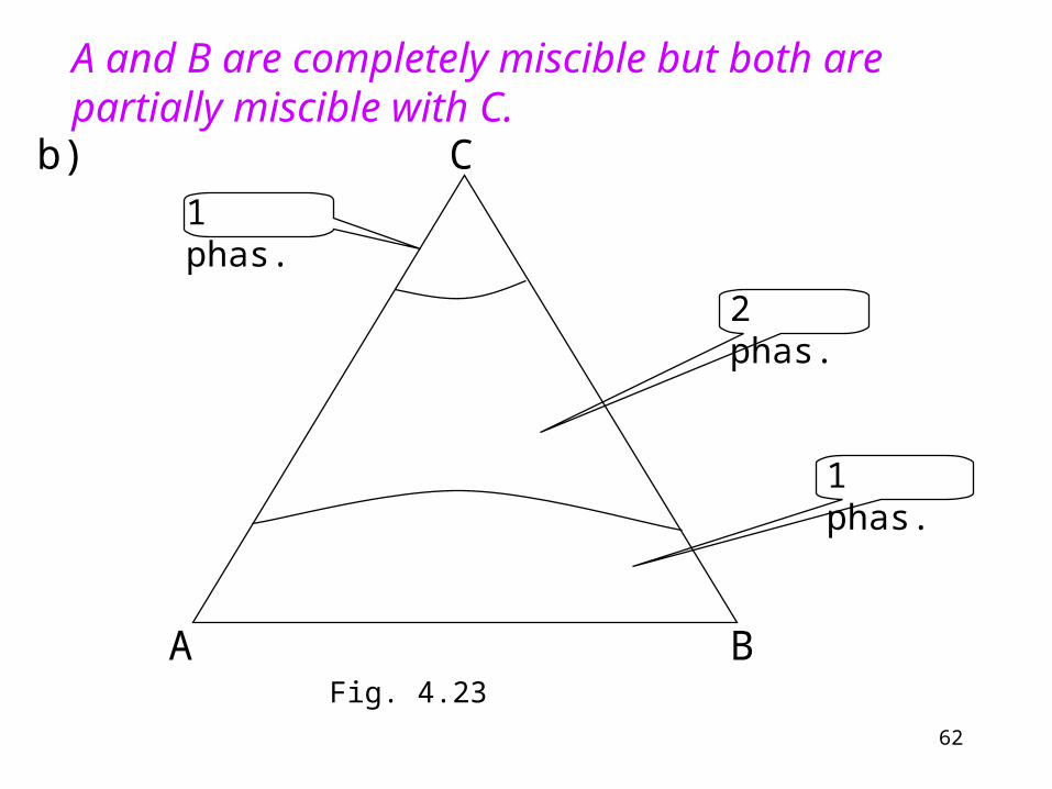
A B
C
1 phas.
2 phas.
1 phas.
b)
A and B are completely miscible but both are partially miscible with C.
Fig. 4.23
63
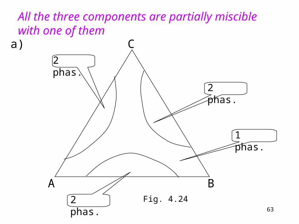
A B
C
1 phas.
2 phas.
2 phas.
2 phas.
All the three components are partially miscible with one of them
a)
Fig. 4.24
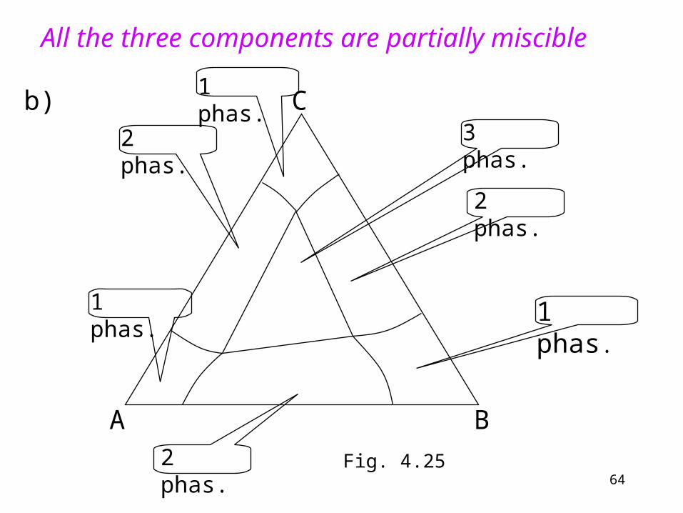
64
A B
C
1 phas.
2 phas.
2 phas.
2 phas.
All the three components are partially miscible
b)3 phas.
1 phas.
1 phas.
Fig. 4.25

65
4.11 Activities and standard states
Expression for the chemical potential:
iii aRT ln0
Standard chemical potential
activity ( always dimensionless)
1.) Ideal gases (partial pressure per standard pressure)
Standard state: p0 pressure ideal behavior
0p
pa i
i
(see 3.25)
66
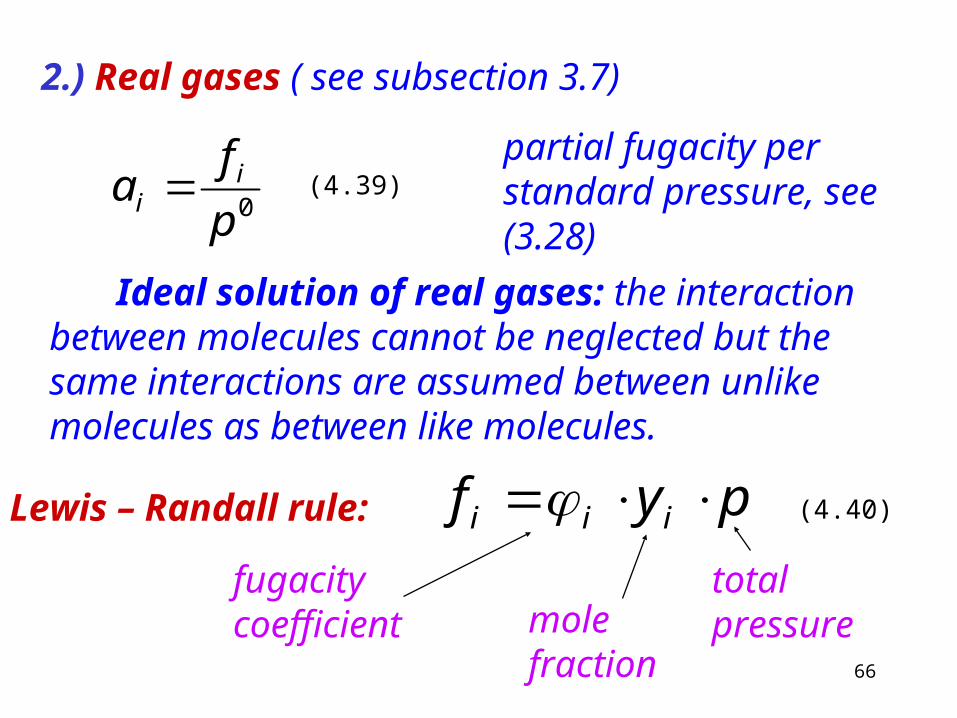
2.) Real gases ( see subsection 3.7)
Ideal solution of real gases: the interaction between molecules cannot be neglected but the same interactions are assumed between unlike molecules as between like molecules.
0p
fa i
i partial fugacity per standard pressure, see (3.28)
Lewis – Randall rule: pyf iii fugacity coefficient mole
fraction
total pressure
(4.39)
(4.40)

67
Standard stateStandard state:: p 1 bary i 1 i 1
fi 1 bar
The ideal gas state at p0 pressure (fugacity) is a fictive state.
00
00 lnln
p
pyRT
p
fRT ii
ii
ii
(4.41)
Expression of the chemical potential for real gases according to (4.40)

68
3.) Solutions1: the component is regarded as solvent. Raoult´s law is applied.
iiii xRTaRT lnln *1
*1
Standard state xi 1xi 1ai xi
This defines the pure liquid at p0 pressure
(4.42)
69
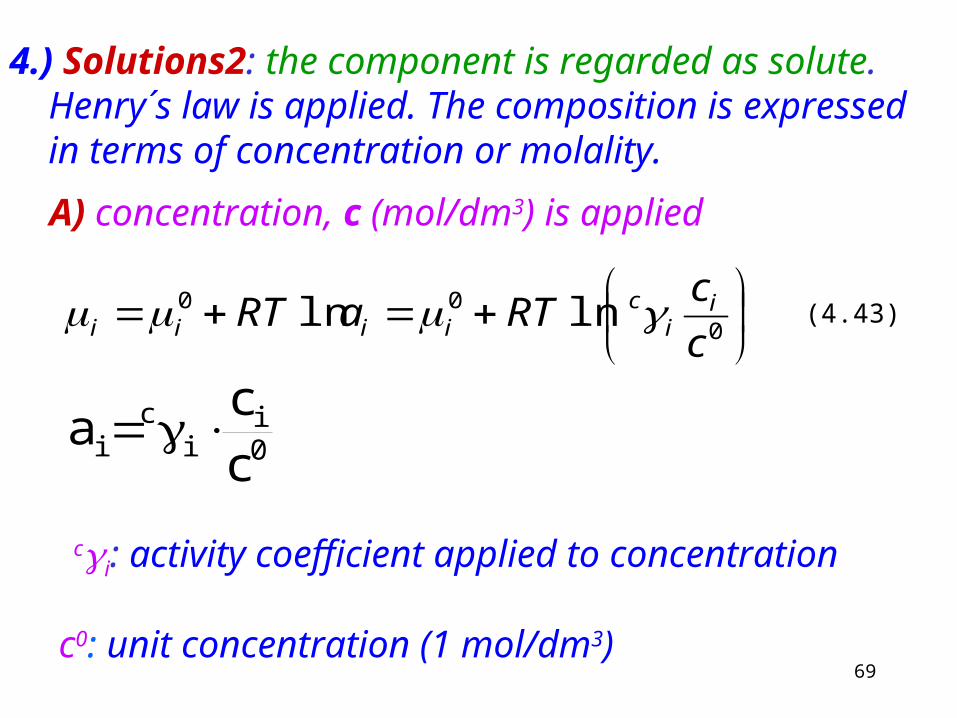
4.) Solutions2: the component is regarded as solute. Henry´s law is applied. The composition is expressed in terms of concentration or molality.
A) concentration, c (mol/dm3) is applied
000 lnln
c
cRTaRT i
ic
iiii
0i
ic
i cc
a
ci: activity coefficient applied to concentration
c0: unit concentration (1 mol/dm3)
(4.43)
70
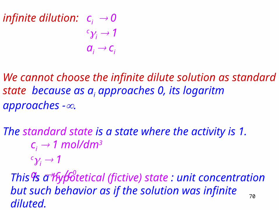
infinite dilution: ci 0ci 1ai ci
We cannot choose the infinite dilute solution as standard state because as ai approaches 0, its logaritm approaches -.
The standard state is a state where the activity is 1.ci 1 mol/dm3
ci 1ai ci /c0
This is a hypotetical (fictive) state : unit concentration but such behavior as if the solution was infinite diluted.
71
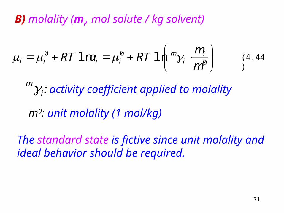
B) molality (mi, mol solute / kg solvent)
000 lnln
m
mRTaRT i
im
iiii
: activity coefficient applied to molality
m0: unit molality (1 mol/kg)
The standard state is fictive since unit molality and ideal behavior should be required.
(4.44)
im
72
4.12 The thermodynamic equilibrium constant
Chemical affinity is the electronic property by which dissimilar chemical species are capable of forming chemical compounds. The following considerations are applied.
1.) In equilibrium at a given temperature and pressure the Gibbs function of the system has a minimum. 2.)The Gibbs function can be expressed in terms of chemical potentials: G = ni i
3.) The chemical potentials depend on the composition (i = i
0 + RT ln ai). In a reaction mixture there is one composition, where the Gibbs function has its minimum. This is the equilibrium composition.
73
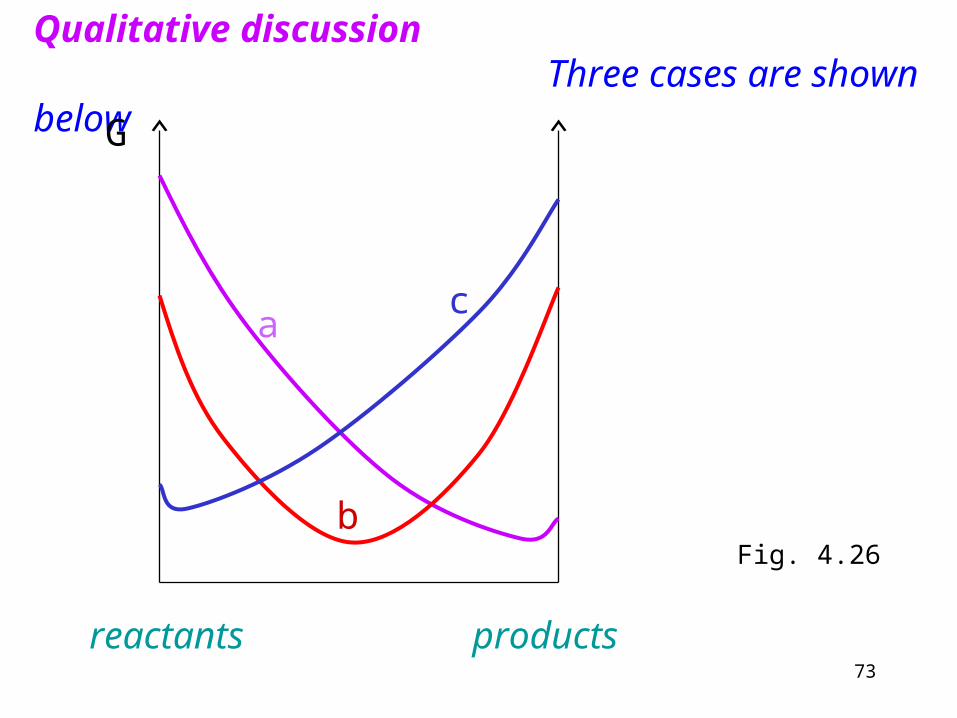
Qualitative discussion Three cases are shown below
G
reactants products
a
b
c
Fig. 4.26
74
a) The equilibrium lies close to pure products. The reaction „goes to completion”.
b) Equilibrium corresponds to reactants and products present in similar proportions.
c) Equilibrium lies close to pure reactants. The reaction „does not go”.
Conclutions:
75
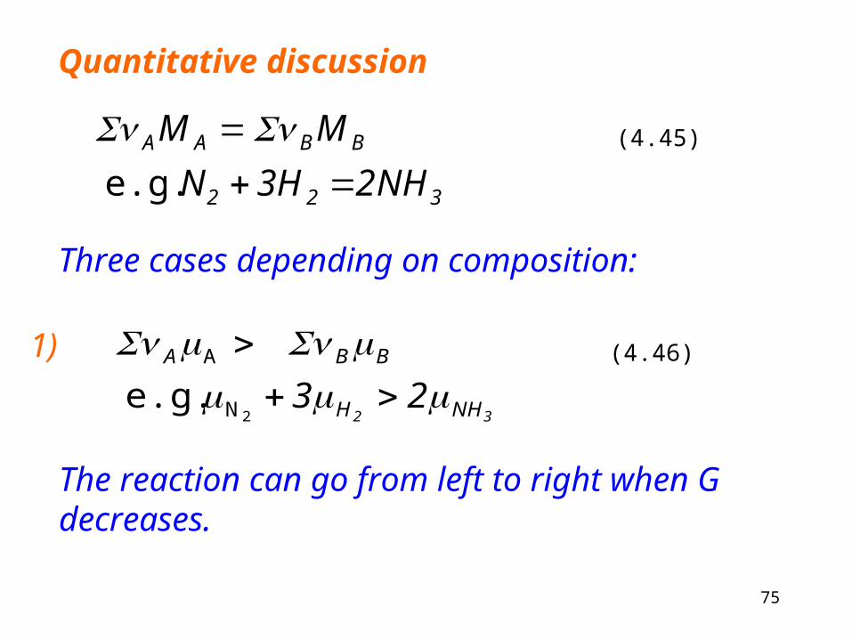
Quantitative discussion
Three cases depending on composition:
1)
The reaction can go from left to right when G decreases.
322
BBAA
NH2H3N
MM
e.g.
(4.45)
32 NHH
BBA
23
2N
A
e.g.
(4.46)
76
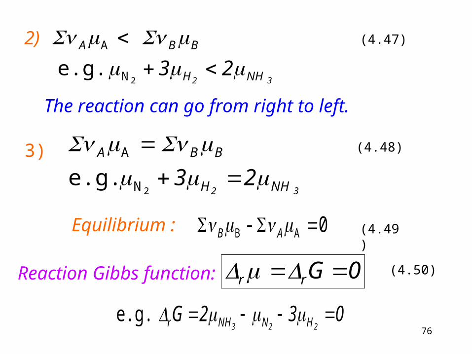
2)
The reaction can go from right to left.
3)
Equilibrium : 0 - AB AB
0Grr Reaction Gibbs function:
032G223 HNNHr e.g.
32 NHH
BBA
23
2N
A
e.g.
(4.47)
32 NHH
BBA
23
2N
A
e.g.
(4.48)
(4.49)
(4.50)
77
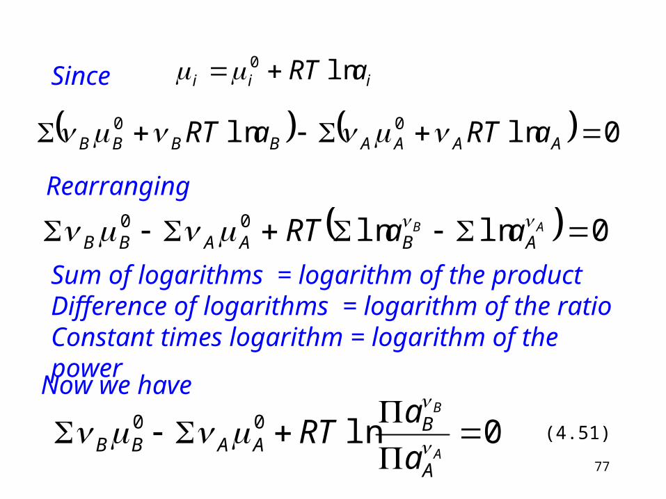
iii aRT ln0
0lnln 00 AAAABBBB aRTaRT
0lnln00 ABABAABB aaRT
Sum of logarithms = logarithm of the productDifference of logarithms = logarithm of the ratioConstant times logarithm = logarithm of the power
0ln00
A
B
A
BAABB a
aRT
Since
Rearranging
Now we have
(4.51)
78
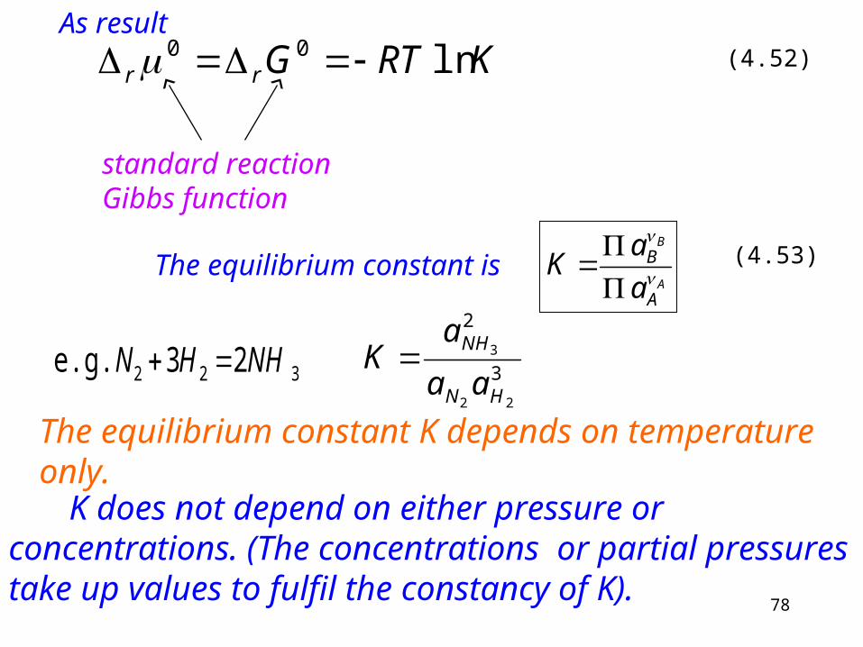
KRTGrr ln00
standard reaction Gibbs function
A
B
A
B
a
aK
3
2
22
3
HN
NH
aa
aK
322 2 3 e.g. NHHN
The equilibrium constant K depends on temperature only.
K does not depend on either pressure or concentrations. (The concentrations or partial pressures take up values to fulfil the constancy of K).
As result
The equilibrium constant is
(4.52)
(4.53)

The equilibrium constant is a very important quantity in thermodynamics that characterizes several types of equilibria of chemical reactions:
in gas, liquid, and solid-liquid phases;
in different types of reactions between
neutral and charged reactants;
The equlibrium constant can be expressed using several parameters like pressure, mole fraction, (chemical) concentration, molality.

80
4.13 Chemical equilibrium in gas phase
A
B
A
B
a
aK
Ideal gases: 0p
pa i
i
A
B
pp
pp
A
B
K
0
0
BA
A
B
pp
pK
A
B
0
0pKK p
: change in number of moleculese.g. SO2 + ½ O2 = SO3
= 1 – 0.5 – 1 = - 0.5
Applications of
Therefore
(4.54)
and(4.55)
A
B
A
Bp p
pK
(4.56)
AB
81
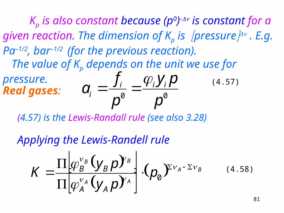
Kp is also constant because (p0)- is constant for a given reaction. The dimension of Kp is pressure . E.g. Pa–1/2, bar–1/2 (for the previous reaction). The value of Kp depends on the unit we use for pressure.Real gases: 00 p
py
p
fa iii
i
(4.57)
BA
AA
BB
ppy
pyK
AA
BB
0
Applying the Lewis-Randell rule
(4.58)
(4.57) is the Lewis-Randall rule (see also 3.28)

82
0ppy
pyK
A
B
A
B
A
B
A
B
0pKKK p
Constant, depends on T only. This is the “true” equilibrium constant.
They depend on pressure but their product does not.
or(4.59)
Extending (4.55) for real gases:
(4.60)
83
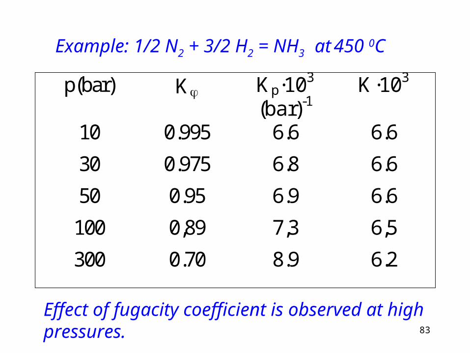
Example: 1/2 N2 + 3/2 H2 = NH3 at 450 0C
p(bar) K Kp·103 (bar)-1
K·103
10 0.995 6.6 6.6
30 0.975 6.8 6.6
50 0.95 6.9 6.6
100 0,89 7,3 6,5
300 0.70 8.9 6.2
Effect of fugacity coefficient is observed at high pressures.

84
4.14 Effect of pressure on equilibrium
The equilibrium constant is independent of pressure. On the other hand, the equilibrium composition in a gas reaction can be influenced by the pressure.
Assume that the participants are ideal gases. According to (4.54a)
A
B
pp
pp
KA
B
0
0
Dalton´s law: pi = yi·p
We express K with gas mole fractions:
85
0
0
0
p
pK
ppy
ppy
K y
A
B
A
B
AB
A
B
A
By y
yK
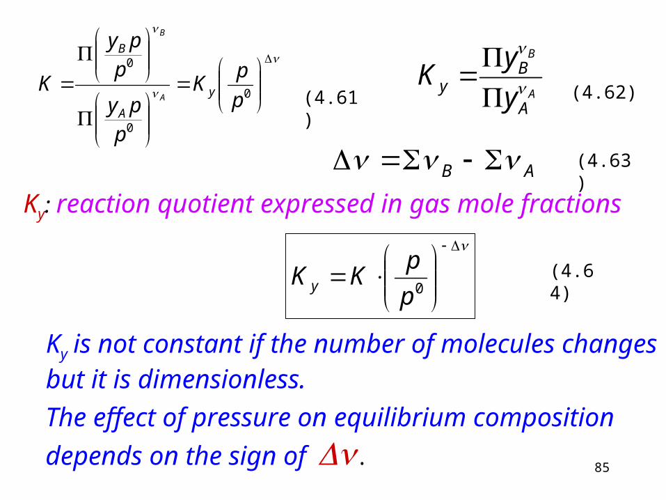
Ky: reaction quotient expressed in gas mole fractions
0p
pKK y
Ky is not constant if the number of molecules changes but it is dimensionless.
The effect of pressure on equilibrium composition
depends on the sign of .
(4.61) (4.62)
(4.63)
(4.64)
86
If 0 (the number of molecules increases), increasing the pressure, decreases Ky, that is, the equilibrium shifts towards the reactants (- is exponent!). If 0 (the number of molecules decreases), decreasing the pressure, favours the products (Ky increases).
Principle of Le Chatelier: a system at equilibrium, when subjected to a perturbation, responds in a way that tends to minimize its effect.
Equilibrium gas reaction: Increasing the pressure, the equilibrium shifts towards the direction where the number of molecules decreases.
87
Reactions where the volume decreases at constant pressure ( < 0) are to be performed at high pressure.
Reactions where the volume increases at constant pressure ( > 0) are to be performed at low pressure or in presence of an inert gas.
For exampleN2 + 3 H2 = 2NH3 = -2Several hundred bars are used.

88
4.15 Gas - solid chemical equilibrium
Heterogeneous reaction: at least one of the reactants or products is in a different phase.
Gas - solid heterogeneous reactions are very important in industry. For example:
C(s) + CO2 (g) = 2 CO (g) CaCO3(s) = CaO (s) + CO2 (g)
89
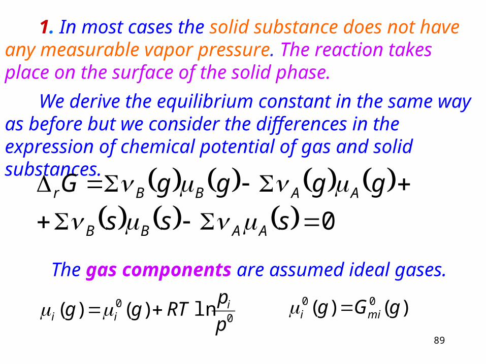
1. In most cases the solid substance does not have any measurable vapor pressure. The reaction takes place on the surface of the solid phase.
We derive the equilibrium constant in the same way as before but we consider the differences in the expression of chemical potential of gas and solid substances.
The gas components are assumed ideal gases.
00 ln)()(
p
pRTgg i
ii )()( 00 gGg mii
0
sss
ggggG
AABB
AABBr

90
The solid components are pure solids, their concentration does not change: i(s) = Gmi(s)
Assume that the molar Gibbs function of a solid does not depend on pressure.
Pressure dependence of G
dG = Vdp – SdT (see 2.19a)
m
T
m Vp
G
In case of solids the molar volume (Vm) is smallE.g. C(graphite):
mol/m1033.5mol/cm33.5cm/g25.2
mol/g12V 363
3m
(see 2.19b)
91
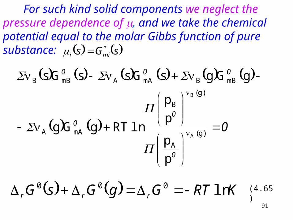
For such kind solid components we neglect the pressure dependence of , and we take the chemical potential equal to the molar Gibbs function of pure substance:
KRTGgGsG rrr ln000
0
0
00
000
)g(
A
)g(
B
mAA
mBBmAAmBB
A
B
p
p
p
p
lnRTgGg
gGgsGssGs
sGs *mii
(4.65)
92
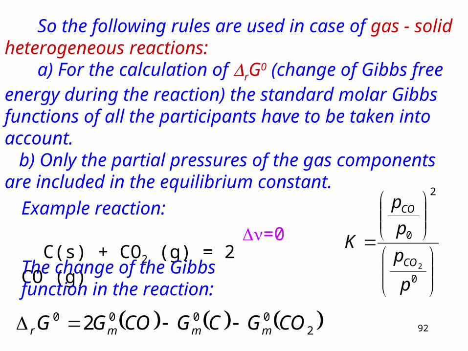
So the following rules are used in case of gas - solid heterogeneous reactions: a) For the calculation of rG0 (change of Gibbs free energy during the reaction) the standard molar Gibbs functions of all the participants have to be taken into account. b) Only the partial pressures of the gas components are included in the equilibrium constant.
Example reaction: C(s) + CO2 (g) = 2 CO (g)
20000 2 COGCGCOGG mmmr
0
2
0
2
p
p
p
p
KCO
CO
The change of the Gibbs function in the reaction:
=0
93
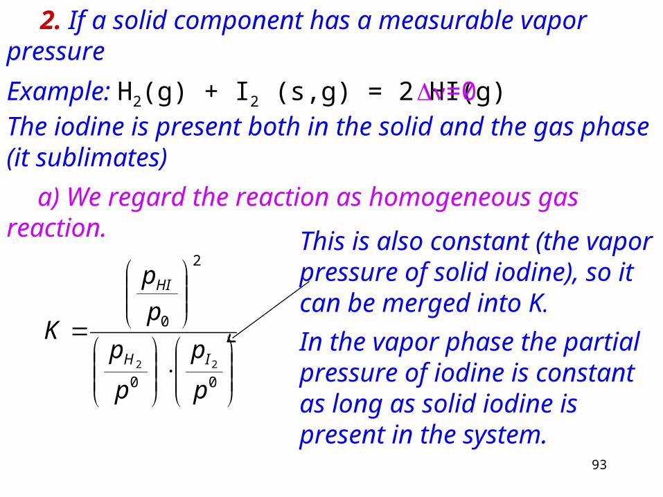
2. If a solid component has a measurable vapor pressure
Example: H2(g) + I2 (s,g) = 2 HI(g) The iodine is present both in the solid and the gas phase (it sublimates)
a) We regard the reaction as homogeneous gas reaction.
00
2
0
22
p
p
p
p
p
p
KIH
HI
This is also constant (the vapor pressure of solid iodine), so it can be merged into K.
In the vapor phase the partial pressure of iodine is constant as long as solid iodine is present in the system.
=0
94
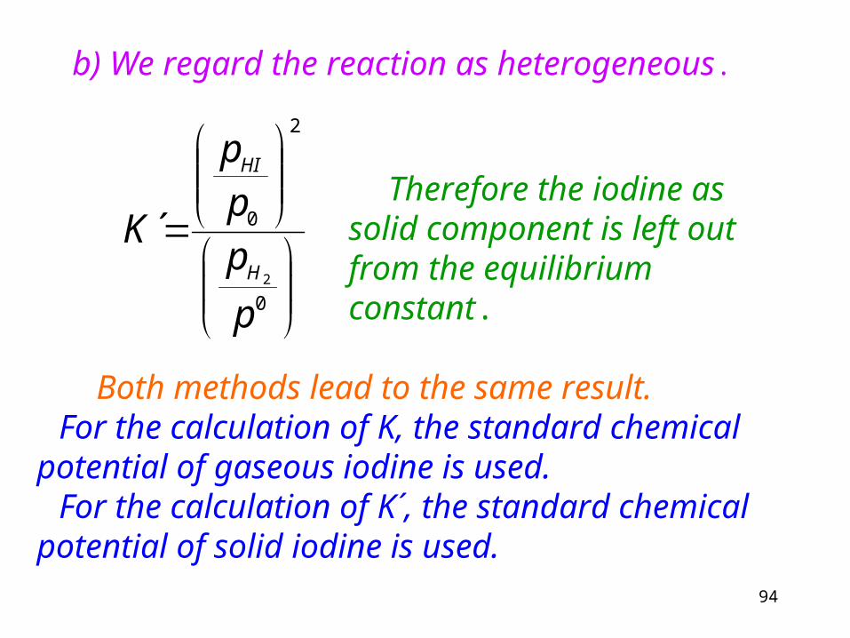
b) We regard the reaction as heterogeneous.
0
2
0
2
´
p
ppp
KH
HI
Both methods lead to the same result. For the calculation of K, the standard chemical potential of gaseous iodine is used. For the calculation of K´, the standard chemical potential of solid iodine is used.
Therefore the iodine as solid component is left out from the equilibrium constant.

95
4.16 Chemical equilibria in liquid state
We study three cases.
1.The components are present in high concentration (e.g. reactions between organic liquids). Such equilibrium reaction is the formation of esters. Equations (4.52) and (4.53):
KRTGr ln0 A
B
A
B
a
aK
The composition is expressed in terms of mole fraction.
iix
i xa A
B
A
B
a
aK
xKKK (4.66a,b,c)
96
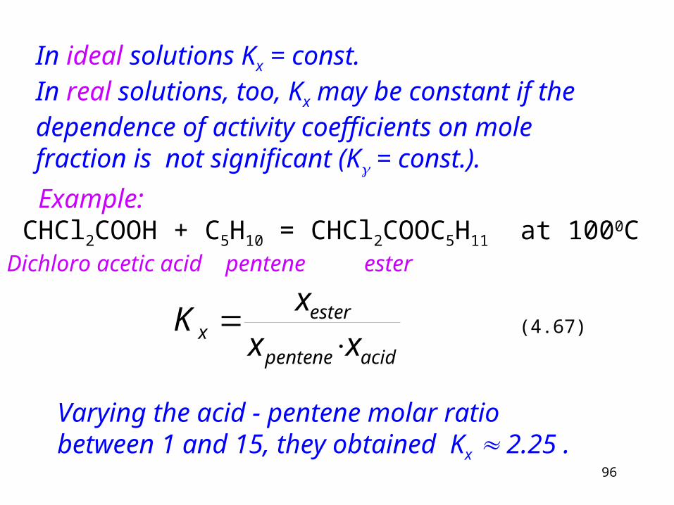
In ideal solutions Kx = const.In real solutions, too, Kx may be constant if the dependence of activity coefficients on mole fraction is not significant (K = const.).
Example: CHCl2COOH + C5H10 = CHCl2COOC5H11 at 1000CDichloro acetic acid pentene ester
acidpentene
esterx xx
xK
Varying the acid - pentene molar ratio between 1 and 15, they obtained Kx 2.25 .
(4.67)
97
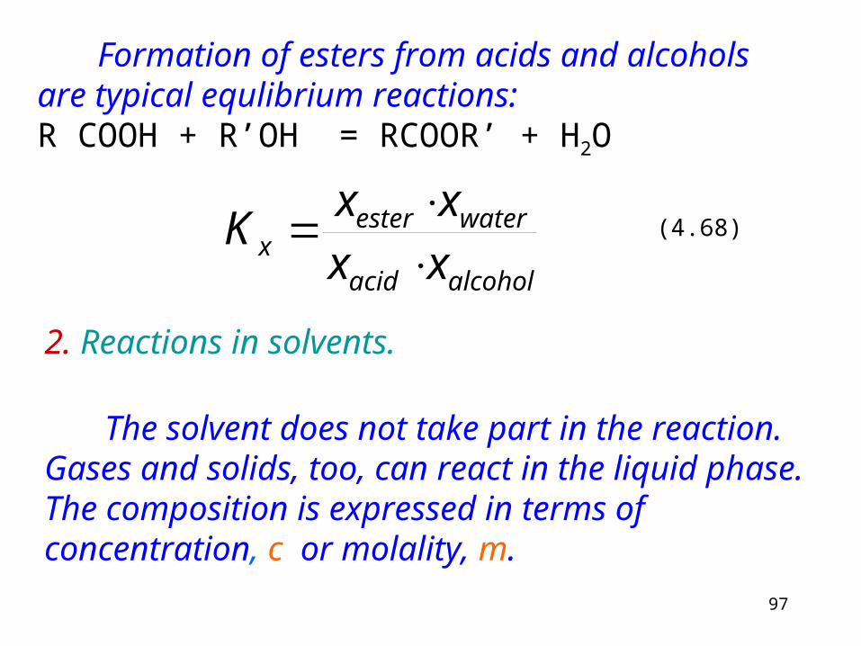
Formation of esters from acids and alcohols are typical equlibrium reactions:R COOH + R’OH = RCOOR’ + H2O
alcoholacid
wateresterx xx
xxK
2. Reactions in solvents.
The solvent does not take part in the reaction. Gases and solids, too, can react in the liquid phase. The composition is expressed in terms of concentration, c or molality, m.
(4.68)
98
00 ln
c
cRT ii
c
ii
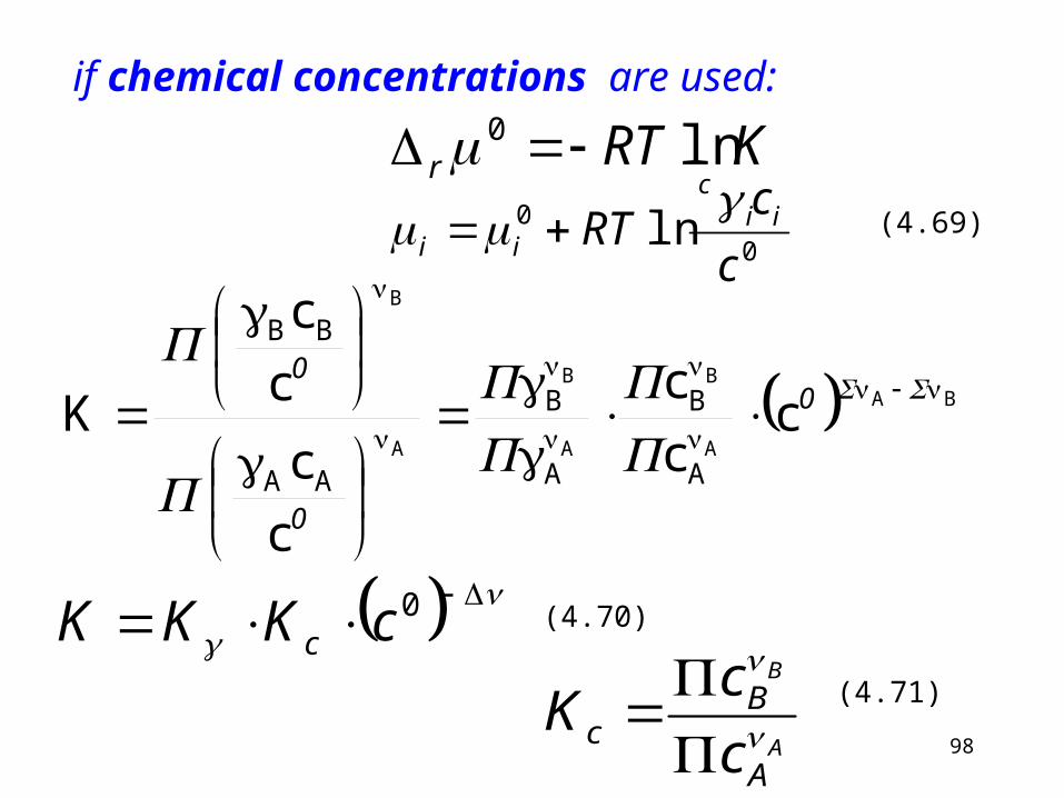
if chemical concentrations are used:
KRTr ln0
0cKKK c
A
B
A
Bc c
cK
BA
A
B
A
B
A
B
cc
c
c
c
c
c
KA
B
A
B
AA
BB
0
0
0
(4.69)
(4.70)
(4.71)
99
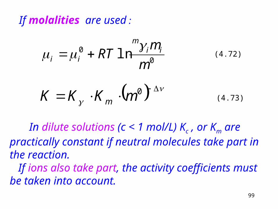
If molalities are used :
00 ln
m
mRT ii
m
ii
0mKKK m
In dilute solutions (c < 1 mol/L) Kc , or Km are practically constant if neutral molecules take part in the reaction. If ions also take part, the activity coefficients must be taken into account.
(4.72)
(4.73)

100
3. Equilibrium in electrolytes.
Even very dilute solutions cannot be regarded ideal (because of the strong electrostatic interaction between ions). Still Kc can be frequently used as equilibrium constant (it is assumed that the activity coefficients are independent of concentration, so K is taken constant).
Dissociation equilibrium
KA = K+ + A-
K+: cation A-: anion
c0(1-) c0· c0· c0 : initial concentration degree of dissociation
1
02c
Kc 0 1
(4.74)
(4.75)
101
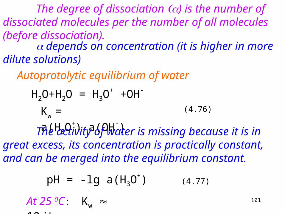
The degree of dissociation ) is the number of dissociated molecules per the number of all molecules (before dissociation). depends on concentration (it is higher in more dilute solutions)
Autoprotolytic equilibrium of water
H2O+H2O = H3O+ +OH-
Kw = a(H3O+)·a(OH-)
The activity of water is missing because it is in great excess, its concentration is practically constant, and can be merged into the equilibrium constant.
At 25 0C: Kw 10-14
pH = -lg a(H3O+)
(4.76)
(4.77)
102
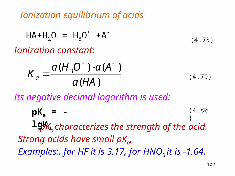
Ionization equilibrium of acids
HA+H2O = H3O+ +A-
)(
)()( 3
HAa
AaOHaKa
Ionization constant:
Its negative decimal logarithm is used:
pKa = - lgKa
pKa characterizes the strength of the acid. Strong acids have small pKa, Examples:. for HF it is 3.17, for HNO3 it is -1.64.
(4.78)
(4.79)
(4.80)
103
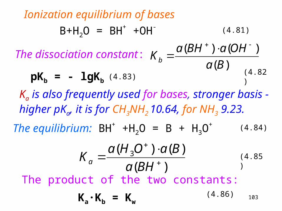
Ionization equilibrium of bases
B+H2O = BH+ +OH-
)(
)()(
Ba
OHaBHaKb
The dissociation constant:
Ka is also frequently used for bases, stronger basis - higher pKa, it is for CH3NH2 10.64, for NH3 9.23.
The equilibrium: BH+ +H2O = B + H3O+
)(
)()( 3
BHa
BaOHaKa
pKb = - lgKb
The product of the two constants:
Ka·Kb = Kw
(4.81)
(4.82)(4.83)
(4.84)
(4.85)
(4.86)

104
4.17 Temperature dependence of the equilibrium constant
The following equation shows that the equilibrium constant depends on temperature only.
KRTGr ln0
The standard chemical potentials depend on temperature only:
Derive lnK with respect to temperature
T
G
RK r
01ln
T
G
TRT
K r01ln
(see 4.52)
105
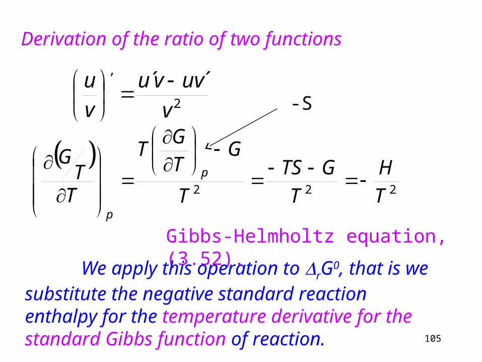
Derivation of the ratio of two functions
2
,´´
v
uvvu
v
u
222 T
H
T
GTS
T
GT
GT
TT
Gp
p
Gibbs-Helmholtz equation, (3.52).
We apply this operation to rG0, that is we substitute the negative standard reaction enthalpy for the temperature derivative for the standard Gibbs function of reaction.
-S
106
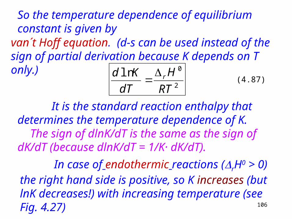
So the temperature dependence of equilibrium constant is given by
It is the standard reaction enthalpy that determines the temperature dependence of K. The sign of dlnK/dT is the same as the sign of dK/dT (because dlnK/dT = 1/K· dK/dT).
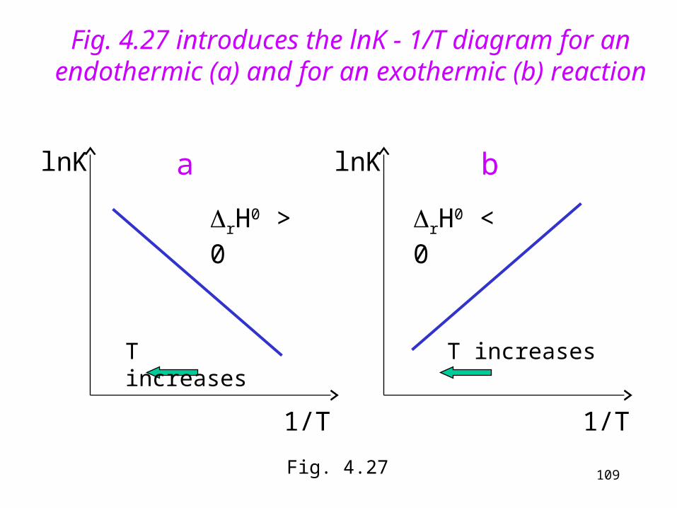
In case of endothermic reactions (rH0 > 0) the right hand side is positive, so K increases (but lnK decreases!) with increasing temperature (see Fig. 4.27)
van´t Hoff equation. (d-s can be used instead of the sign of partial derivation because K depends on T only.)
2
0ln
RT
H
dT
Kd r (4.87)
107
In case of exothermic reactions (rH0 <0) K decreases (but lnK increases!) with increasing temperature (see Fig. 4.27)
Principle of Le Chatelier: The equilibrium shifts towards the endothermic direction if the temperature is raised, and in the exothermic direction if the temperature is lowered, endothermic: heat is absorbed form the environment, exothermic: heat is transmitted to the environment.
For exothermic reactions low temperature favours the equilibrium but at too low temperatures the rate of reaction becomes very low. We must find an optimum temperature.
For exact integration of van´t Hoff equation we must know the temperature dependence of the standard enthalpy of reaction.

108
In a not too large temperature range the reaction enthalpy is assumed constant. Then integration is easy:
.ln0
constRT
HK r
If we plot the logarithm of the equilibrium constant against the reciprocal of the absolute temperature, we optain a linear function. The slope is determined by the standard reaction enthalpy.
(4.88)
109
Fig. 4.27 introduces the lnK - 1/T diagram for an endothermic (a) and for an exothermic (b) reaction
alnK
1/T
rH0 > 0
T increases
b
1/T
rH0 < 0
lnK
T increases
Fig. 4.27