1 a different view of the lattice boltzmann method for simulating fluid flow jeremy levesley robert...
TRANSCRIPT
1
A different view of the Lattice Boltzmann method for simulating fluid flow
Jeremy LevesleyRobert BrownleeAlexander Gorban
University of Leicester, UK
Supported by EPSRC
June 27th 2007 Dundee 2007 2
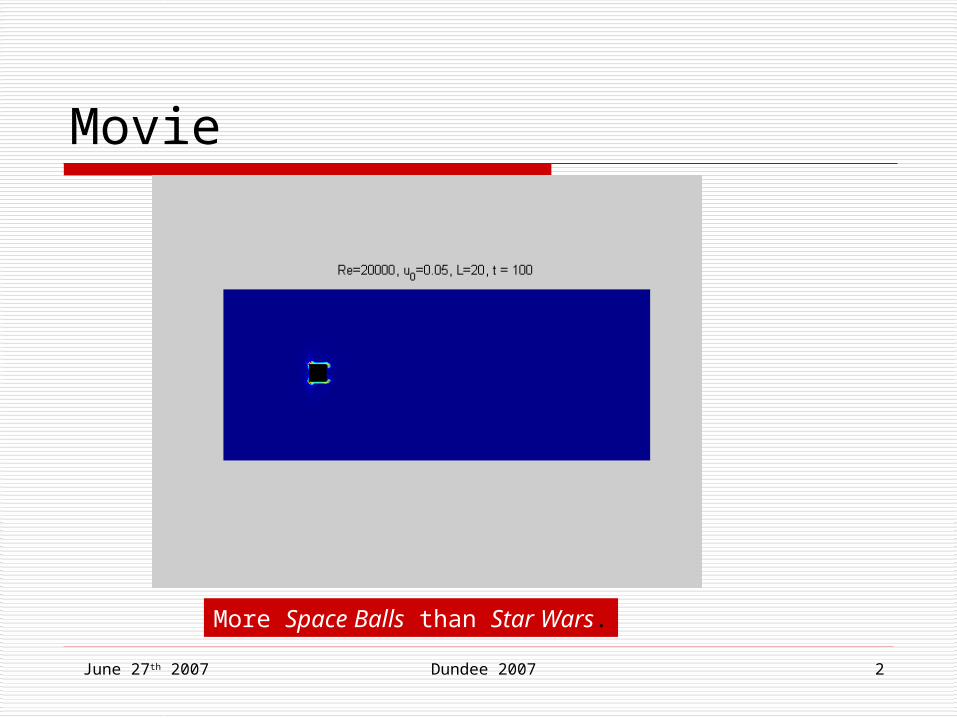
Movie
More Space Balls than Star Wars.
June 27th 2007 Dundee 2007 3
High Reynold’s Number Flow
Very low viscosity leads to complicated dynamics.
PDE model for such flows is the Navier-Stokes equation with small viscosity, the Euler equation for zero one.
Examples of shock tube, square cylinder, lid-driven cavity.
June 27th 2007 Dundee 2007 4
Talk
A new framework for looking at LBM. Not the Boltzmann equation.
It is close to the Navier-Stokes’ equations in some sense.
Stabilisation of method via targetted introduction of diffusion.
Filters and entropy limiters.
June 27th 2007 Dundee 2007 5
Fraud and hypocrite Approximation theorist
talking about “PDEs” Numerical analysis
conference – what is the order of convergence of your method?
Spot the hypocracy.
June 27th 2007 Dundee 2007 6
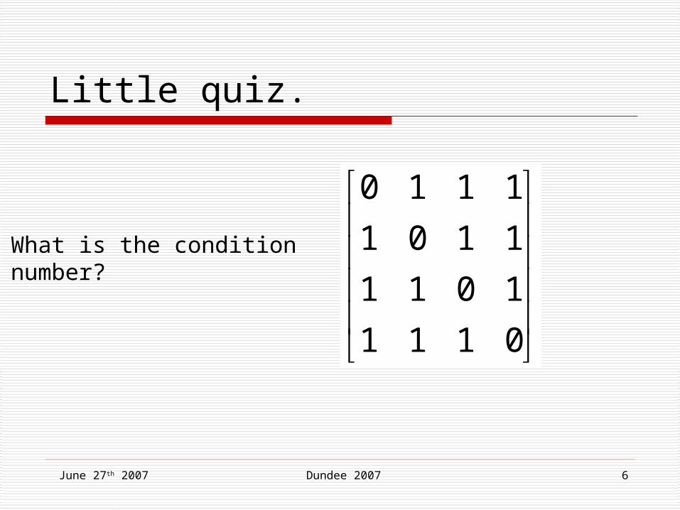
Little quiz.
0111
1011
1101
1110
What is the condition number?
June 27th 2007 Dundee 2007 7
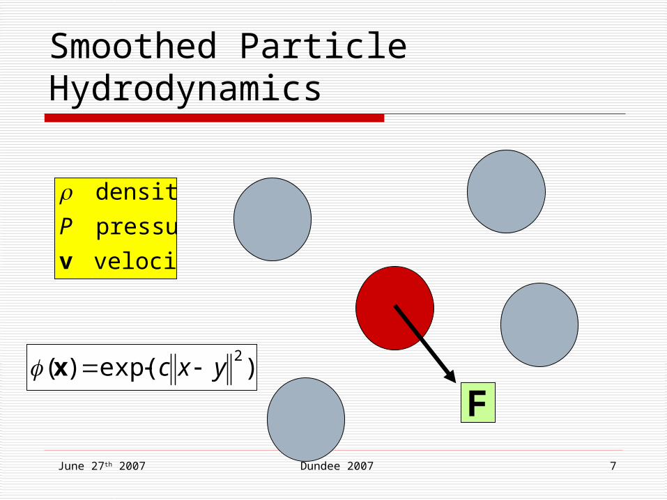
Smoothed Particle Hydrodynamics
velocity
pressure
density
v
P
F)exp()(
2yxc x
June 27th 2007 Dundee 2007 8
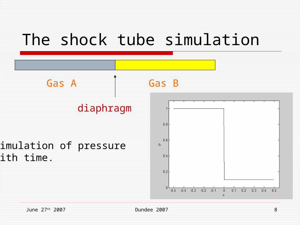
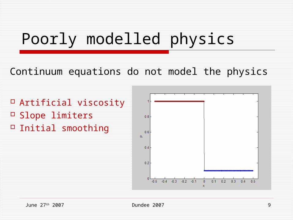
The shock tube simulation
Gas A Gas B
diaphragm
Simulation of pressurewith time.
June 27th 2007 Dundee 2007 9
Poorly modelled physics
Artificial viscosity Slope limiters Initial smoothing
Continuum equations do not model the physics
June 27th 2007 Dundee 2007 10
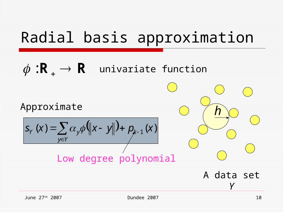
Radial basis approximation
RR : univariate function
A data set Y
Approximate
)()( 1 xpyxxs kYy
yY
Low degree polynomial
h
June 27th 2007 Dundee 2007 11
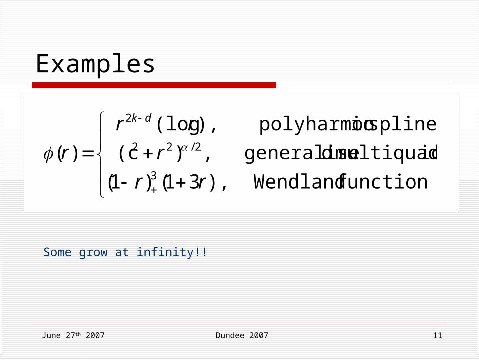
Examples
function Wendland
icmultiquadr dgeneralise
spline icpolyharmon
),31()1(
,)(c
),(log
)(3
2/22
2
rr
r
rr
r
dk
Some grow at infinity!!
June 27th 2007 Dundee 2007 12
Micchelli (1986, CA) Interpolation problem is always
solvable. In all space dimensions For any configuration of points (with
some very mild restrictions). A great challenge to find appropriate
methods for solving real high dimensional problems.
June 27th 2007 Dundee 2007 13
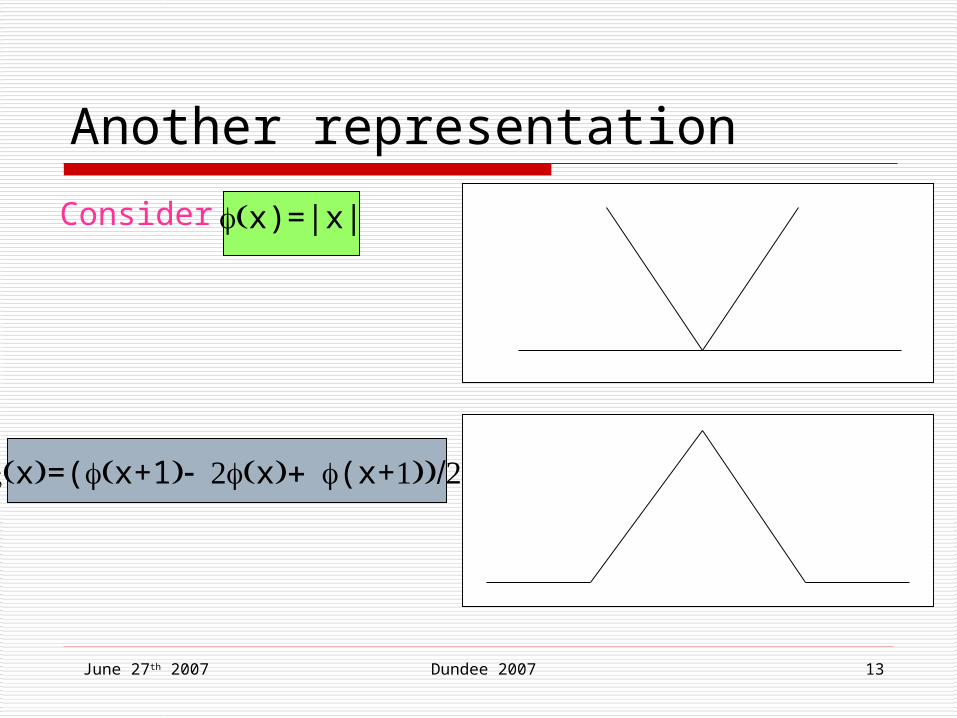
Another representation
Consider
x=(x+1x(x+
x)=|x|
June 27th 2007 Dundee 2007 14
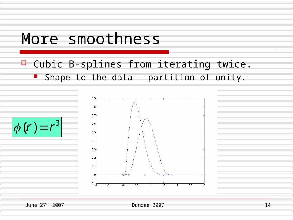
More smoothness
Cubic B-splines from iterating twice. Shape to the data – partition of unity.
3)( rr
June 27th 2007 Dundee 2007 15
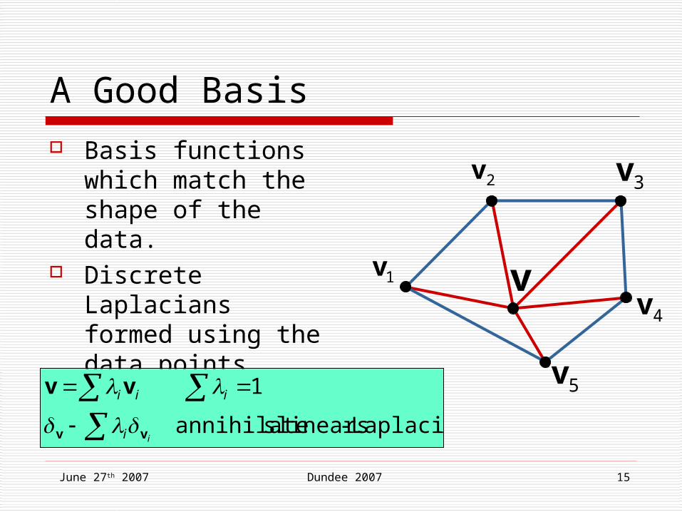
A Good Basis Basis functions
which match the shape of the data.
Discrete Laplacians formed using the data points.
2v
v1v
3v
4v
5v
Laplacian - linears sannihilate
1
ii
iii
vv
vv
June 27th 2007 Dundee 2007 16
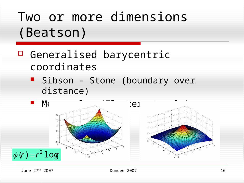
Two or more dimensions (Beatson)
Generalised barycentric coordinates Sibson – Stone (boundary over distance) Mean value (Floater et. al.)
rrr log)( 2
June 27th 2007 Dundee 2007 17
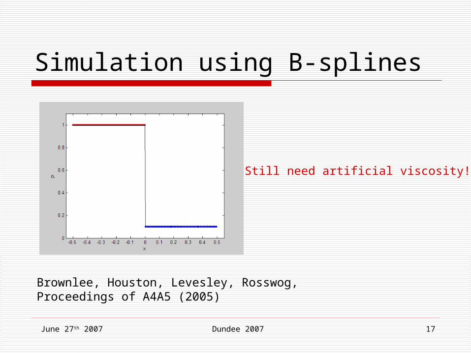
Simulation using B-splines
Still need artificial viscosity!!
Brownlee, Houston, Levesley, Rosswog, Proceedings of A4A5 (2005)
June 27th 2007 Dundee 2007 18
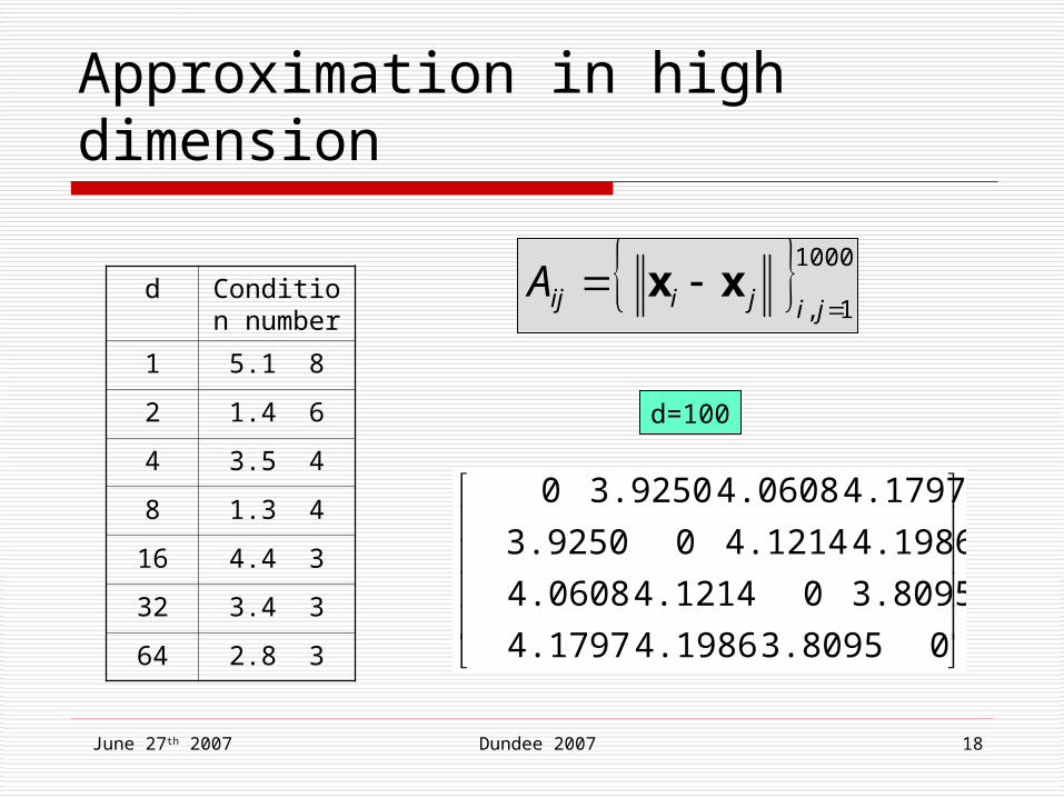
Approximation in high dimension
0 3.8095 4.1986 4.1797
3.8095 0 4.1214 4.0608
4.1986 4.1214 0 3.9250
4.1797 4.0608 3.9250 0
d Condition number
1 5.1 8
2 1.4 6
4 3.5 4
8 1.3 4
16 4.4 3
32 3.4 3
64 2.8 3
d=100
1000
1,
jijiijA xx
June 27th 2007 Dundee 2007 19
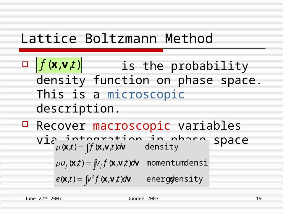
Lattice Boltzmann Method
is the probability density function on phase space. This is a microscopic description.
Recover macroscopic variables via integration in phase space
),,( tf vx
densityenergy ),,(),(
density momentum),,(),(
density),,(),(
2
vvxx
vvxx
vvxx
dtfvte
dtfvtu
dtft
jj
June 27th 2007 Dundee 2007 20
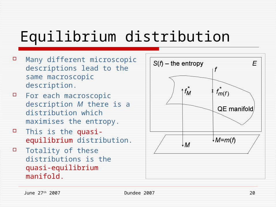
Equilibrium distribution Many different microscopic
descriptions lead to the same macroscopic description.
For each macroscopic description M there is a distribution which maximises the entropy.
This is the quasi-equilibrium distribution.
Totality of these distributions is the quasi-equilibrium manifold.
June 27th 2007 Dundee 2007 21
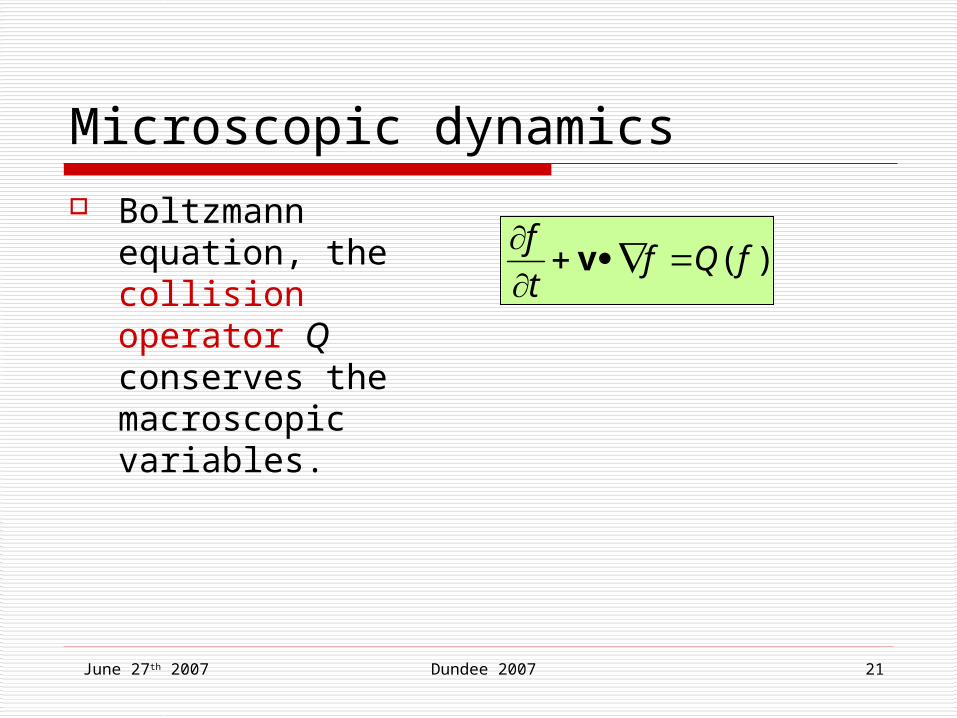
Microscopic dynamics Boltzmann
equation, the collision operator Q conserves the macroscopic variables.
)( fQft
f
v
June 27th 2007 Dundee 2007 22
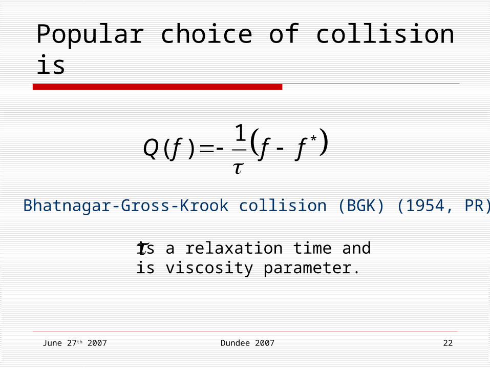
Popular choice of collision is
*1)( fffQ
Bhatnagar-Gross-Krook collision (BGK) (1954, PR)
is a relaxation time and is viscosity parameter.
June 27th 2007 Dundee 2007 23
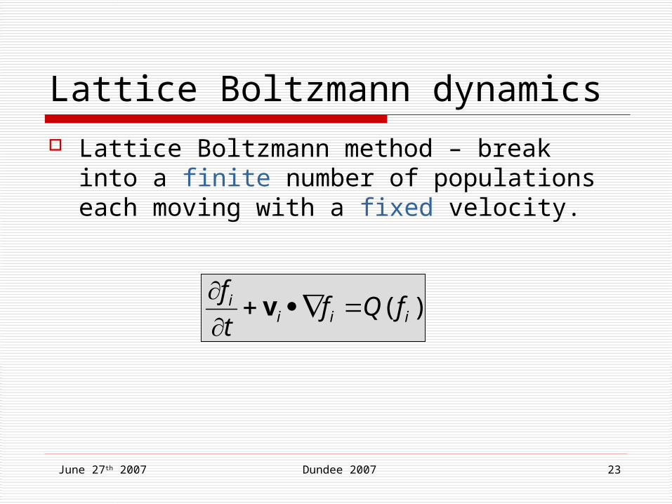
Lattice Boltzmann dynamics
Lattice Boltzmann method – break into a finite number of populations each moving with a fixed velocity.
)( iiii fQft
f
v
June 27th 2007 Dundee 2007 24
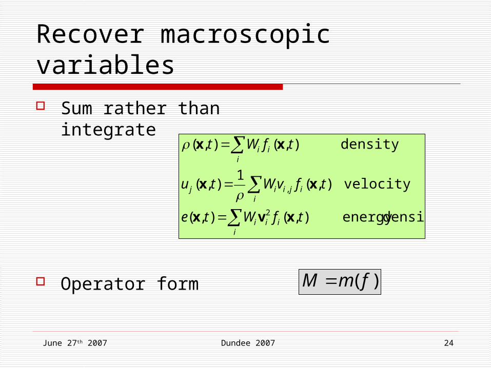
Recover macroscopic variables Sum rather than
integrate
Operator form
densityenergy ),(),(
velocity),(1
),(
density ),(),(
2
,
iiii
iijiij
iii
tfWte
tfvWtu
tfWt
xvx
xx
xx
)( fmM
June 27th 2007 Dundee 2007 25
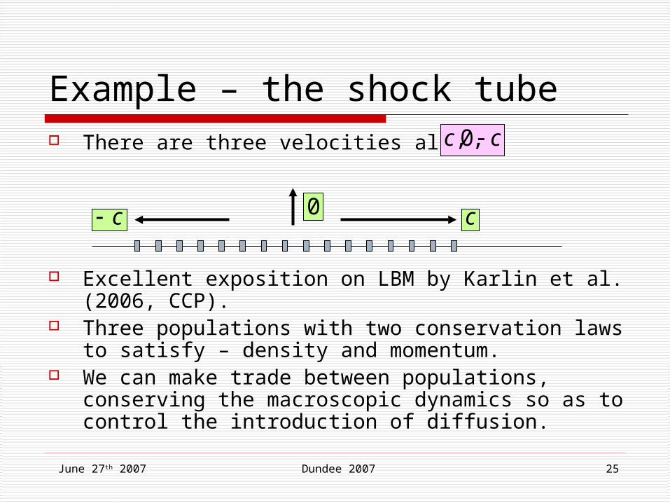
Example – the shock tube There are three velocities allowed
Excellent exposition on LBM by Karlin et al. (2006, CCP).
Three populations with two conservation laws to satisfy – density and momentum.
We can make trade between populations, conserving the macroscopic dynamics so as to control the introduction of diffusion.
cc ,0,
0c c
June 27th 2007 Dundee 2007 26
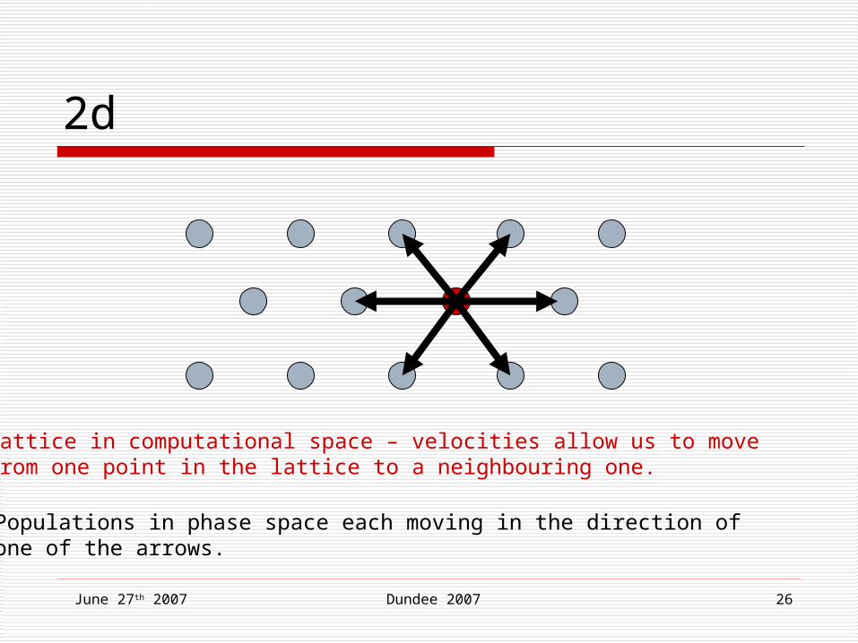
2d
Lattice in computational space – velocities allow us to movefrom one point in the lattice to a neighbouring one.
Populations in phase space each moving in the direction ofone of the arrows.

June 27th 2007 Dundee 2007 27
Numerical discretisation
)'(12
)()(2
')',()(1
),(),(
3
*
tQt
tQttQt
dttxfxftxftttvxftt
t
High Reynolds number has tending to 0.
3
1)'(
tQ
3
t
June 27th 2007 Dundee 2007 28
Either
High viscosity and we can approximate the Boltzmann equation.
Or Low viscosity and we cannot let time
step get less than without incurring huge computational cost.
Not approximating Boltzmann!!

June 27th 2007 Dundee 2007 29
New idea Simulate transport equation by
Free flying for time t Equilibration
Macroscopic variables are transported by free flight.
Microscopic variable redistributed leaving macroscopic variables locally unchanged.
Smallness parameter is t.

June 27th 2007 Dundee 2007 30
“Nonlinearity is local, non-locality is linear”
(Sauro Succi)Moreover, non-locality is linear,
exact and explicit

June 27th 2007 Dundee 2007 31
Numerically
iii
iiii
fff
tftftttf
~
),(~
2),(),( xxvx
Numerical scheme is
Free flight Equilibration
(ELBM)entropy equal
mequilibriu toreturned21
(LBGK)limit viscosityzero1

June 27th 2007 Dundee 2007 32
Stability problem is nontrivial: Entropic LBM does not solve it
ELBM
LBGK
Shock tube 1D test {-c,0,c}.

June 27th 2007 Dundee 2007 33
Coarse-graining the Ehrenfests’ way
Formal kinetic equation
Microscopic dynamics
)( fJdt
df
))((1 iti ff
ffJdt
df v)(
t

June 27th 2007 Dundee 2007 34
Macroscopic dynamics
Match the microscopic and macroscopic dynamics to order
),( tMFdt
dM
))(()( *fmtM t
2t
***
)(2
))(( PffJDmt
fJmdt
dMff
Euler Navier-Stokes

June 27th 2007 Dundee 2007 35
Summarise
Free fly for time and equilibrate populations f*
Integrate to recover macroscopic variables
Navier-Stokes’ equations to order with viscosity
t
2t2/t

June 27th 2007 Dundee 2007 36
Coupled steps – a scheme of LBM stabilization
QE manifold
Free flight steps t
Overrelaxation step
Complete relaxation(Ehrenfests’ step)
The mirror image
f0
f1
f *-(f1-f*)f *-(2β-1)(f1-f*)
f *
f2

June 27th 2007 Dundee 2007 37
Decoupled viscosity from timestep
***
)()())(( PffJDmfJmdt
dMff
Controlled viscosity

June 27th 2007 Dundee 2007 38
Shock tube 1D test {-1,0,1}
LBGK
ELBM
magicsteps

June 27th 2007 Dundee 2007 39
The Ehrenfests’ Step Potential problem near shocks where we are
too far from the quasi equilibrium.
0f
too big
1f

June 27th 2007 Dundee 2007 40
Not enough artificial dissipation LBGK and
ELBM Step back from mirror. Not enough dissipation.
Ehrenfest Introduces dissipation in a very precise and targetted way.
0f1f
mirrordissipation
0f
1f dissipation

June 27th 2007 Dundee 2007 41
Simulation looks good

June 27th 2007 Dundee 2007 42
Simulation of square cylinder

June 27th 2007 Dundee 2007 43
Relationship for Strouhal number and Reynold’s number
Okajima’s experiment (1982) ….
LBM simulations, Ansumali et. al.(2004)
Ehrenfest’s steps(2006)

June 27th 2007 Dundee 2007 44
Lid-driven cavity flow with ES(movie of vorticity)
(k,δ)=(32,10-3)

June 27th 2007 Dundee 2007 45
Flux limiters
S.K. Godunov (1959) we should choose between spurious oscillation in high order non-monotone scheme and additional dissipation in first order scheme.
Flux limiter schemes are invented as the “formulas of compromise” to combine high resolution schemes in areas with smooth fields and first-order schemes in areas with sharp gradients.
The additional dissipation control is difficult.

June 27th 2007 Dundee 2007 46
Nonequilibrium entropy limiters for LBM
Entropy is a scalar quantity Entropy trimming: we monitor local deviation of f from the
correspondent equilibrium f*, and correct most nonequilibrium states (with highest ΔS(f)=S(f*)-S(f));
0f
too big
1fEhrenfest

June 27th 2007 Dundee 2007 47
Positivity rule
f *
f
f *+(2β-1)(f*-f)
Positivity fixation
Positivity domain

June 27th 2007 Dundee 2007 48
Entropy Filtering
)))((( ** fffSffF
Ehrenfest
.,0
,,1)(
dt
dtt

June 27th 2007 Dundee 2007 49
Median Filter Choose a number of neighbouring points. Arrange the non-equilibrium entropies in order of
size. Choose middle one.
Very robust and gentle in places where signal is smooth.
Preserves edges, but reduces oscillation.

June 27th 2007 Dundee 2007 50
Lid driven cavity For Re < 7000
steady flow For Re > 8500
periodic flow Bifurcation point
between
Peng, Shiau, Hwang (2003)
(100 by 100 grid)
3007402

June 27th 2007 Dundee 2007 51
Velocity at monitor point
Reynolds’ number7375

June 27th 2007 Dundee 2007 52
Locating bifurcation point
Re=7135

June 27th 2007 Dundee 2007 53
Conclusions Navier-Stokes’ equations arise naturally via
free flight and equilibration in phase space. The viscosity, both actual and artificial can
be controlled precisely. The appropriate notion of smallness is the
free-flight time, which is a computational, not physical number.
Non-locality is exact and computable, non-linearity is local.
Reproduce statistics in some standard tests. Flux limiting can be done via control of a
scalar variable entropy.