1 a multi-relational approach to spatial classification richard frank school of computing science...
TRANSCRIPT

1
A Multi-Relational Approach to Spatial Classification
Richard FrankSchool of Computing Science Simon Fraser UniversityBurnaby BC, [email protected]
Martin EsterSchool of Computing Science Simon Fraser UniversityBurnaby BC, [email protected]
Arno KnobbeLIACS, Leiden UniversityLeiden, the [email protected]

2MOTIVATION
• Why are some malls profitable?
• Why are some houses burgled?• Good location? • Expensive neighbourhood?• Close to major roads?
• Learn classifiers given• Location• Feature values• Neighbouring locations • Features of neighbours
• Use classifier to predict label of unknown entities
Burnaby, British Columbia, Canada
Burgled Houses

3
• Spatial data seems to have multi-relational (MR) aspects• MR classification techniques cannot be applied directly to spatial data
• With MR data the relationships between the entities are explicitly given• Spatial relationships are only implied via the entity’s spatial location• Non-spatial aggregation cannot deal with spatial dependencies• Many relationships large search space
INTRODUCTION
5STEPS
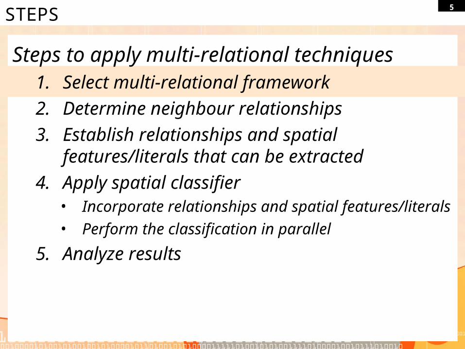
Steps to apply multi-relational techniques1. Select multi-relational framework
2. Determine neighbour relationships
3. Establish relationships and spatial features/literals that can be extracted
4. Apply spatial classifier• Incorporate relationships and spatial features/literals• Perform the classification in parallel
5. Analyze results
6MULTI-RELATIONAL CLASSIFICATION
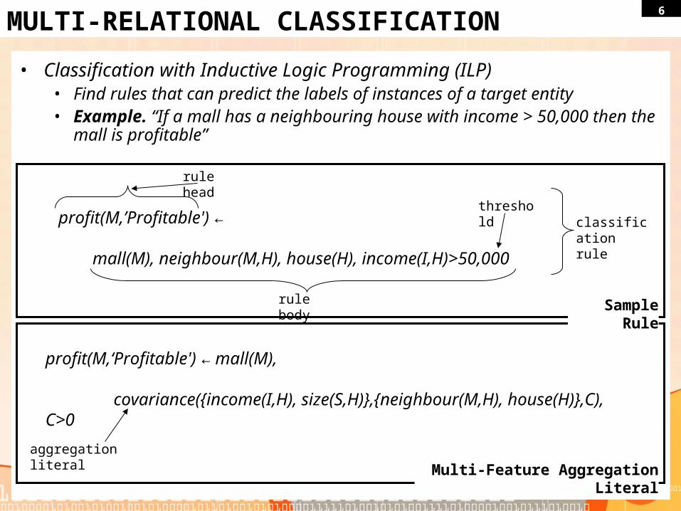
• Classification with Inductive Logic Programming (ILP)• Find rules that can predict the labels of instances of a target entity• Example. “If a mall has a neighbouring house with income > 50,000 then the
mall is profitable”
profit(M,’Profitable') ←
mall(M), neighbour(M,H), house(H), income(I,H)>50,000
rule body
threshold
rule head
classification rule
Multi-Feature Aggregation Literal
Sample Rule
profit(M,‘Profitable') ← mall(M),
covariance({income(I,H), size(S,H)},{neighbour(M,H), house(H)},C), C>0
aggregation literal

7STEPS
Steps to apply multi-relational techniques1. Select multi-relational framework
2. Determine neighbour relationships
3. Establish relationships and spatial features/literals that can be extracted
4. Apply spatial classifier• Incorporates relationships and spatial features/literals• Performs the classification in parallel
5. Analyze results
8NEIGHBOURHOOD DEFINITIONS
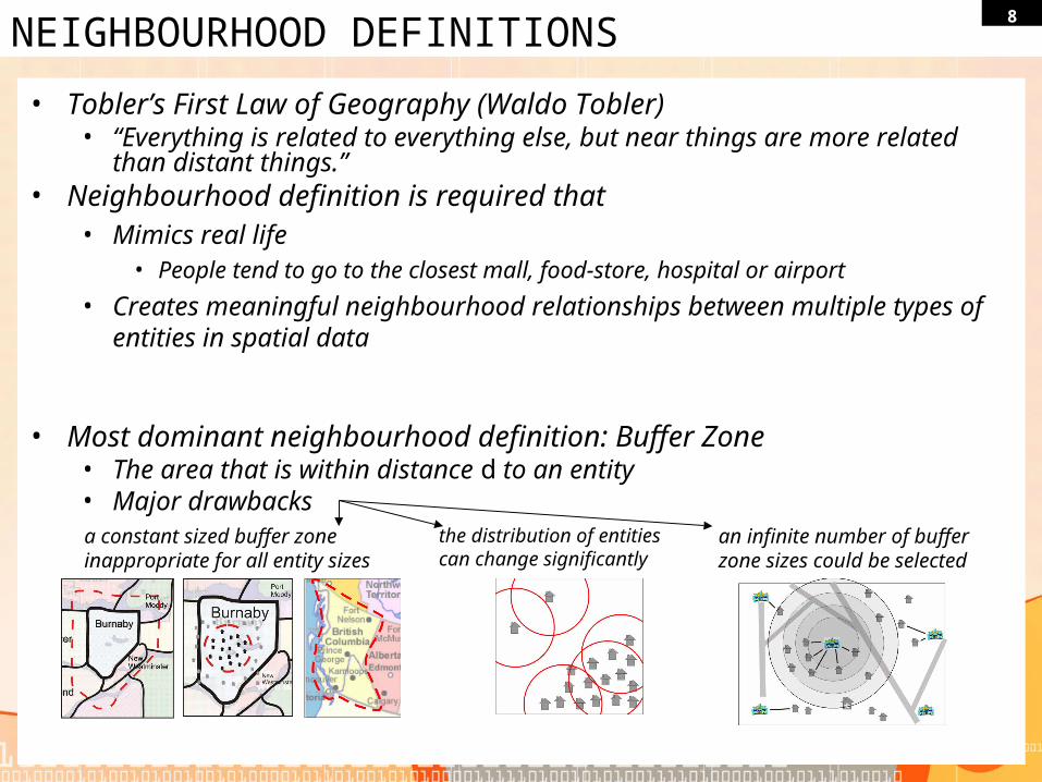
• Tobler’s First Law of Geography (Waldo Tobler)• “Everything is related to everything else, but near things are more related than
distant things.”• Neighbourhood definition is required that
• Mimics real life• People tend to go to the closest mall, food-store, hospital or airport
• Creates meaningful neighbourhood relationships between multiple types of entities in spatial data
• Most dominant neighbourhood definition: Buffer Zone• The area that is within distance d to an entity• Major drawbacks
a constant sized buffer zone inappropriate for all entity sizes
the distribution of entities can change significantly
an infinite number of buffer zone sizes could be selected

9VORONOI NEIGHBOURHOOD
• Voronoi Diagrams• Defined and Named after
Georgy Feodosevich Voronoy• Partition a plane into regions• Region contains area closest to
the entity in the Voronoi cell• Naturally represent relationships
between entities• Completely data-driven – no
user parameter
• Can be computed for • point data (e.g. houses)• segment data (e.g. roads)• areal data (e.g. lakes)
Voronoi diagram for Houses
Voronoi diagram for Malls

10
• Voronoi Neighbourhood Definition• Two entities, A and B, are neighbours iff:
• A intersects the Voronoi cell of B or B intersects the Voronoi cell of A, and A and B are of different types, or,
• the Voronoi cells of A and B are adjacent, and A and B are of the same type
Neighbourhood relationships
VORONOI NEIGHBOURHOOD
11STEPS
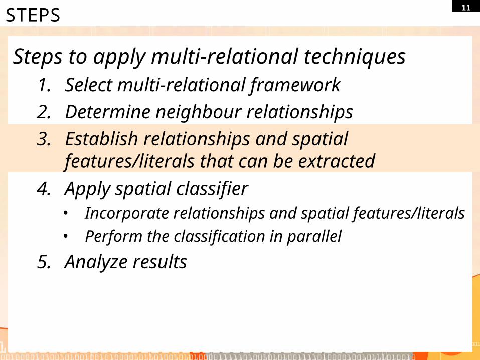
Steps to apply multi-relational techniques1. Select multi-relational framework
2. Determine neighbour relationships
3. Establish relationships and spatial features/literals that can be extracted
4. Apply spatial classifier• Incorporate relationships and spatial features/literals• Perform the classification in parallel
5. Analyze results
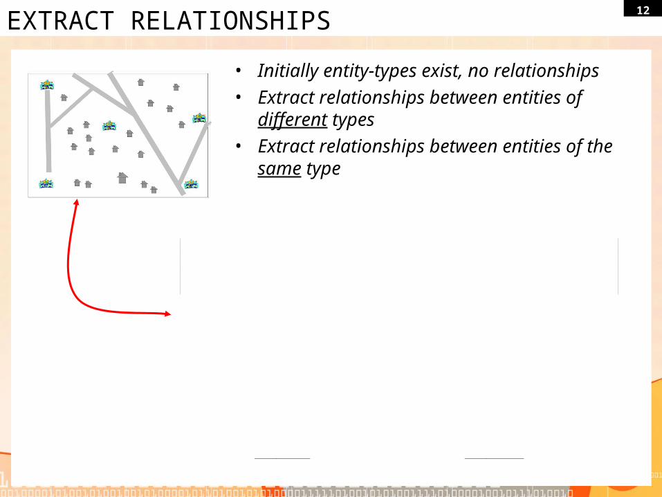
12EXTRACT RELATIONSHIPS
• Initially entity-types exist, no relationships• Extract relationships between entities of different
types• Extract relationships between entities of the
same type
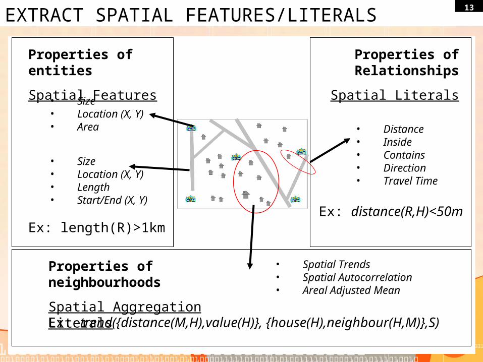
13EXTRACT SPATIAL FEATURES/LITERALS
• Size• Location (X, Y)• Area
• Size• Location (X, Y)• Length• Start/End (X, Y)
Properties of entities
Spatial Features
• Distance• Inside• Contains• Direction• Travel Time
Properties of Relationships
Spatial Literals
Ex: length(R)>1kmEx: distance(R,H)<50m
Properties of neighbourhoods
Spatial Aggregation Literals
• Spatial Trends• Spatial Autocorrelation• Areal Adjusted Mean
Ex: trend({distance(M,H),value(H)}, {house(H),neighbour(H,M)},S)

14STEPS
Steps to apply multi-relational techniques1. Select multi-relational framework
2. Determine neighbour relationships
3. Establish relationships and spatial features/literals that can be extracted
4. Apply spatial classifier• Incorporate relationships and spatial features/literals• Perform the classification in parallel
5. Analyze results

15
• Unified Multi-relational Aggregation-based Spatial Classifier (UnMASC)• Multi-relational based spatial classification algorithm• Two-class problem• Based on the idea of the sequential covering algorithm
• Sequential covering algorithm• Generate one rule at a time• Refine rule by adding literals• Start new rule when rule-termination condition applies• Once a rule is finalised
• Entities covered are removed• Another rule is started
RULE LEARNING – OVERVIEW
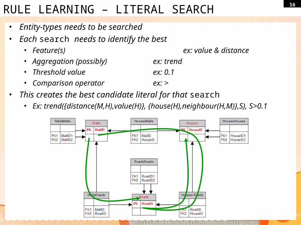
16RULE LEARNING – LITERAL SEARCH
• Entity-types needs to be searched• Each search needs to identify the best
• Feature(s) ex: value & distance
• Aggregation (possibly) ex: trend
• Threshold value ex: 0.1
• Comparison operator ex: >
• This creates the best candidate literal for that search• Ex: trend({distance(M,H),value(H)}, {house(H),neighbour(H,M)},S), S>0.1
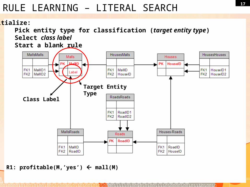
17RULE LEARNING – LITERAL SEARCH
Initialize:Pick entity type for classification (target entity type)Select class labelStart a blank rule
Class Label
Target Entity Type
R1: profitable(M,’yes’) mall(M)

18RULE LEARNING – LITERAL SEARCH
Rule 1 – Iteration 1:Search the entity-types referenced in rule for best feature Search neighbours of entity-types referenced in rule for best featureAdd best feature to the rule
R1: profitable(M,’yes’) mall(M), TREND({D, V}, {house(H), neighbour(M,H), value(H, V), distance(M,H)}, S), S > 0
R1: profitable(M,’yes’) mall(M)
size

19RULE LEARNING – LITERAL SEARCH
Rule 1 – Iteration 2:Search the entity-types referenced in rule for best feature Search neighbours of entity-types referenced in rule for best featureAdd best feature to the rule
R1: profitable(M,’yes’) mall(M), TREND({D, V}, {house(H), neighbour(M,H), value(H, V), distance(M,H)}, S), S > 0
type
, neighbour(R, H), type(R)=‘highway’

20
• Number of searches increases as rule length increases
RULE LEARNING – LITERAL SEARCH
Iteration 2{Malls}{Malls, Malls}{Malls, Houses}{Malls, Roads}{Malls, Houses, Malls}{Malls, Houses, Roads}{Malls, Houses, Houses}Searches: 7
Iteration 1{Malls}{Malls, Malls}{Malls, Houses}{Malls, Roads}Searches: 4
Iteration 3{Malls}{Malls, Malls}{Malls, Houses}{Malls, Roads}{Malls, Houses, Malls}{Malls, Houses, Roads}{Malls, Houses, Houses}{Malls, Houses, Roads, Malls}{Malls, Houses, Roads, Houses}{Malls, Houses, Roads, Roads}Searches: 10
21PARALLEL SEARCH
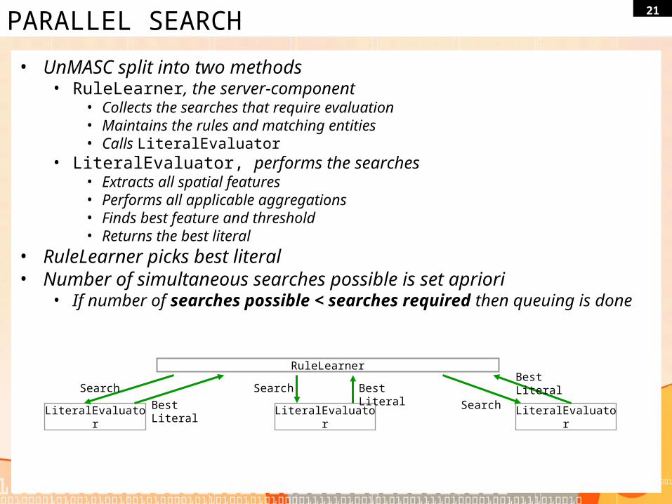
• UnMASC split into two methods• RuleLearner, the server-component
• Collects the searches that require evaluation• Maintains the rules and matching entities• Calls LiteralEvaluator
• LiteralEvaluator, performs the searches• Extracts all spatial features• Performs all applicable aggregations• Finds best feature and threshold• Returns the best literal
• RuleLearner picks best literal• Number of simultaneous searches possible is set apriori
• If number of searches possible < searches required then queuing is done
RuleLearner
LiteralEvaluator LiteralEvaluator LiteralEvaluator
Search Search
SearchBest Literal
Best LiteralBest Literal

22PARALLEL SEARCH – OPTIMIZATION
• Search sizes are different• For example
• {Malls}: expected to be small • Only a few malls in a city• No aggregations are involved
• {Malls} < {Malls, Houses}• Many houses in a city• Houses must be aggregated over their neighbouring malls
• {Malls} < {Malls, Roads} < {Malls, Houses}• Aggregation has to occur• |roads| < |houses|
• Very costly search can execute last• Estimate cost of each search based on
• Number of entities in target table• Features of entities• Number of relationships between entities used in rule
• Reprioritize queue execute costly search first
23STEPS
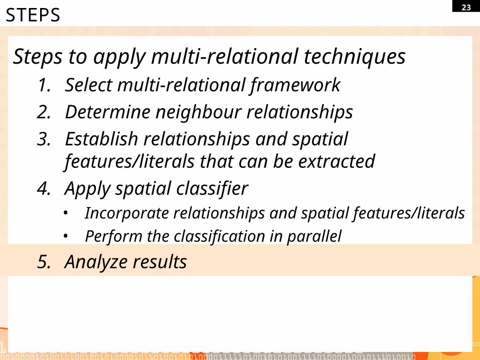
Steps to apply multi-relational techniques1. Select multi-relational framework
2. Determine neighbour relationships
3. Establish relationships and spatial features/literals that can be extracted
4. Apply spatial classifier• Incorporate relationships and spatial features/literals• Perform the classification in parallel
5. Analyze results

24EXPERIMENTS
• Dataset• Real-world crime data
• Collaboration with the Criminology Department at Simon Fraser University• For the Royal Canadian Mounted Police (RCMP) in British Columbia (BC) • Between August 1, 2001 and August 1, 2006• Location of crime• Type of crime
• British Columbia Assessment Authority (BCAA) dataset• Containing the property values of all plots of land within BC
• The city of Burnaby, BC was selected • 66,000 entities• Types of entities & counters
• Each property was labelled• Burglary exists or not

25EXPERIMENTS
• UnMASC was evaluated using three experiments
• Neighbour using Buffer zones• 2.8 million spatial relationships between entities
• Neighbour using Voronoi neighbourhoods • 3.8 million spatial relationships
• Use only the target entity type • no neighbouring entity types are evaluated
• Effectiveness of the parallelization of UnMASC• Parallel (6 threads) • Serial (1 thread)
• 5-fold cross-validation was performed
26EXPERIMENTS
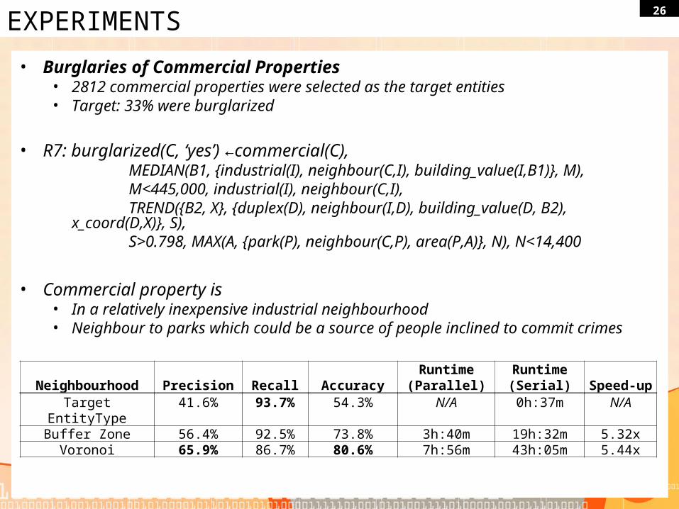
• Burglaries of Commercial Properties• 2812 commercial properties were selected as the target entities• Target: 33% were burglarized
• R7: burglarized(C, ‘yes’) ←commercial(C), MEDIAN(B1, {industrial(I), neighbour(C,I), building_value(I,B1)}, M), M<445,000, industrial(I), neighbour(C,I), TREND({B2, X}, {duplex(D), neighbour(I,D), building_value(D, B2),
x_coord(D,X)}, S), S>0.798, MAX(A, {park(P), neighbour(C,P), area(P,A)}, N),
N<14,400
• Commercial property is• In a relatively inexpensive industrial neighbourhood• Neighbour to parks which could be a source of people inclined to commit crimes
Neighbourhood Precision Recall AccuracyRuntime (Parallel)
Runtime (Serial) Speed-up
Target EntityType 41.6% 93.7% 54.3% N/A 0h:37m N/ABuffer Zone 56.4% 92.5% 73.8% 3h:40m 19h:32m 5.32x
Voronoi 65.9% 86.7% 80.6% 7h:56m 43h:05m 5.44x

27EXPERIMENTS
• Burglaries of High Rise Properties• 1036 high-rise properties were selected • 44.3% of properties were burglarized
• burglarized(H, ‘yes’) ←highrise(H), • building_value(H,V), V>2,160,000• AVG(D1, {commercial(C), neighbour(H,C), distance(H,C,D1)}, A), A<302• commercial(C), neighbour(H,C),
• MEDIAN(W, {park(P), neighbour(C,P), width(P)}, M1), M1<122• MEDIAN(X, {duplex(D), neighbour(C,D), land_value(D)}, M2), M2>351,500
• Burglarized high-rises are• Expensive • Near high-traffic areas with small parks
Neighbourhood Precision Recall AccuracyRuntime (Parallel)
Runtime (Serial) Speed-up
Target EntityType 57.1% 97.6% 66.4% N/A 0h:4m N/ABuffer Zone 83.4% 87.7% 86.3% 3h:18m 17h:06m 5.18x
Voronoi 85.2% 87.8% 87.7% 4h:31m 23h:37m 5.23x

28CONCLUSION
• Multi-relational approach to spatial classification was presented • Proposed a Voronoi-diagram based
neighbourhood definition • Introduced a formal set of additions to the First
Order Logic framework• Presented a scalable parallel implementation• Showed substantial gains in precision and
accuracy• Demonstrated the importance of selecting the
proper neighbourhood definition

29
Thank you