1 a stochastic geometry approach to the modeling of ieee
TRANSCRIPT

1
A Stochastic Geometry Approach to the
Modeling of IEEE 802.11p for Vehicular Ad
Hoc Networks
Zhen Tong1, Hongsheng Lu2, Martin Haenggi1 and Christian Poellabauer2
Abstract
IEEE 802.11p has become the standard to be used in future vehicular ad hoc networks. However,
most studies on its performance are based on simulations. In this paper, we present a novel analytical
approach based on stochastic geometry. In particular, we extend the Matern hard-core type II process
with a discrete and non-uniform distribution, which is used to derive the temporal states of back-off
counters. By doing so, concurrent transmissions from nodes within the carrier sensing ranges of each
other are taken into account, leading to a more accurate approximation to real network dynamics. A
comparison with ns2 simulations shows that our model achieves a good approximation in networks with
different densities.
Index Terms
IEEE 802.11p, Vehicular Ad Hoc Networks, Queueing Theory, Poisson Point Process, Matern Hard-
core Point Process
I. INTRODUCTION
A. Motivation
Vehicular ad hoc networks (VANETs) are an important component of intelligent transportation
systems, with the goal to improve traffic safety and efficiency. In a VANET, every node (i.e.,
1Zhen Tong and Martin Haenggi are with Department of Electrical Engineering, University of Notre Dame, Notre Dame, IN
46556, USA, E-mail: {ztong1,mhaenggi}@nd.edu2Hongsheng Lu and Christian Poellabauer are with Department of Computer Science and Engineering, University of Notre
Dame, Notre Dame, IN 46556, USA, E-mail: {hlu,cpoellab}@nd.edu
December 6, 2013 DRAFT

2
vehicle) is assumed to broadcast up to 10 safety-related messages a second, where each message
contains GPS information (i.e., a vehicle’s location, speed, and heading). Vehicles that receive
such messages are able to track the senders, which therefore helps avoid vehicular collisions.
In 2010, the IEEE 802.11p [1] amendment to the 802.11 standard was published as the first-
generation media access control and physical layer solution to future VANETs. However, it
suffers from the same problem as other CSMA-based MAC protocols, which have a sharply
decreasing performance as the number of nodes increases. In VANETs, it means a plunging
delivery ratio of safety-related messages to recipients, leading to deteriorated tracking accuracy.
Many efforts have focused on improving the performance of IEEE 802.11p, most of which
are based on simulations [2], [3]. However, the problem is that we cannot simulate every case
or combination of system parameters. A mathematical understanding is needed, to help save
computational cost and provide guidance on the design of novel solutions. Therefore, in this
paper, we use stochastic geometry to explore the modeling and analysis of IEEE 802.11p. In
particular, we would like to devise models that can accurately capture the temporal and spatial
behavior of this CSMA-based protocol for different network configurations.
B. Related Work
A rich body of literature on the performance analysis of CSMA-based networks can be found
in the research community, among which most are based on queueing theory. For example, the
performance of the carrier-sense multiple access with collision avoidance (CSMA/CA) scheme
has been analyzed in [4], [5] using a discrete Markov chain model. Since they only focused
on one-hop networks (where all the nodes are within each other’s carrier sensing range) with
saturated traffic, it was possible to obtain a clear and complete mathematical formula for packet
transmission probability and throughput. Later, researchers tried to apply the same modeling
approach to a broader set of cases [6]–[8], including different types of traffic, various lengths
of buffers, multi-hop networks (where the nodes can be out of each other’s carrier sensing
range) and so forth. In [9], [10], the authors investigated the performance of IEEE 802.11p with
enhanced distributed channel access capability where applications with different priorities are
divided into four access categories (ACs) according to their criticalities for the vehicle’s safety.
Since each AC has a separate back-off process, every AC can be viewed as a "virtual" node
competing against others within a single node and across the other nodes. The authors assumed
December 6, 2013 DRAFT

3
that all the nodes observe the same channel to compute the throughput and delay using queueing
theory, which constitutes an extension of [4], [5]. However, all the resulting models were either
more complicated or only applicable to simplified network topologies.
On the other hand, stochastic geometry, in particular point process theory, has been widely used
in the last decade to provide models and methods to analyze wireless networks, see [11], [12] and
references therein. Stochastic geometry provides a natural way of defining and computing critical
performance metrics of the networks, such as the interference distribution, outage probability and
so forth, by taking into account all potential geometrical patterns for the nodes, in the same way
queueing theory provides response times or congestion, considering all potential arrival patterns.
To our best knowledge, the first paper using stochastic geometry to model the reliability of
IEEE 802.11p protocol is [13]. However, it is limited to the analysis of dense VANETs using
ALOHA to approximate the CSMA-based MAC protocol. Similarly, [14], [15] only focus on the
performance analysis of VANETs using ALOHA as the MAC scheme. The connectivity of the
VANET in urban environment has been studied in [16]. A model based on stochastic geometry
has been developed to obtain the probability of a node to be connected to the origin and the
mean number of connected nodes for a given set of system parameters. However, the model does
not explicitly take into account the temporal dynamics specific to VANETs, which are caused
by factors like periodic traffic and the back-off process in IEEE 802.11p. The Matern hard-core
process of type II [12, Chapter 3] has been used in [17] to analyze dense IEEE 802.11 networks,
in which the nodes’ locations are drawn according to a Poisson point process and the random
back-off counter is modeled as an independent mark that is associated with each node. However,
the mark is assumed to be uniform between [0, 1] which is not the case for IEEE 802.11p since
the back-off counter takes only discrete values from 0 to W , where W is the maximum of
back-off counter (a typical value for W is 15).
C. Contributions
Our main contributions are:
1) We investigate the transmission behavior of vehicular networks using a continuous-time
Markov chain model that is based on a novel combination of queueing theory and point
process theory. We show that the location distribution of the transmitting nodes varies from
December 6, 2013 DRAFT

4
being a hard-core process to being a Cox process [12, Chapter 3] as the network density
increases.
2) A novel Matern hard-core process is proposed to capture the hard-core effect of CSMA and
concurrent transmissions occurring within the same carrier sensing range. In particular, a
modified Matern hard-core process of type II (called Matern-II-discrete process for the rest
of the paper, whereas the original Matern hard-core process of type II is henceforth called
Matern-II-continuous process) is used with a discrete and non-uniform mark distribution
to model the temporal information of the back-off counter and the spatial locations of the
transmitting nodes. In this way, nodes with the same back-off counter value can transmit
at the same time with nonzero probability even if they are within the carrier sensing range
of each other, which makes the model more realistic.
3) We validate the effectiveness of our model by comparing it to others and ns2 simulations
of IEEE 802.11p for both fading and non-fading channels. The results show that our model
can be applied to networks of different densities with good accuracy.
D. Organization
The rest of the paper is organized as follows: Section II introduces the system model. In
Section III, queueing theory and stochastic geometry are used to investigate the distribution of
the transmitting nodes and the back-off counter distribution in networks with different densities.
Section IV proposes and describes the Matern-II-discrete process in detail. The system perfor-
mance is evaluated and compared with other models in Section V. We conclude our work in
Section VI.
II. SYSTEM MODEL
A. Traffic Model
In this study, we assume that all the nodes are placed on a line according to a Poisson point
process (PPP) with intensity λ0. This set of nodes is denoted as Φ. According to IEEE 802.11p,
each node generates 10 messages every second, which is equivalent to the requirement to transmit
a message every 100 ms. A message is dropped if it has not been sent out before a new one
arrives. Since the message is beneficial for every vehicle around, broadcast is used, which means
no RTS/CTS is exchanged before transmissions. More specifically, when a message is available
December 6, 2013 DRAFT

5
at a node, if the channel is idle, the message is broadcast immediately. Otherwise, a back-off
counter in [W ] , {0, 1, · · · ,W} is drawn uniformly at random. W + 1 is called the contention
window size; it is fixed since no ACK feedback is used.
A node has to go through a back-off process if it cannot send the message immediately, i.e., if
its back-off counter is set. As shown in Fig. 1 when the channel becomes idle, the node decreases
its back-off counter value immediately by one. It keeps doing so afterwards each time a time
interval δ elapses (δ is called the slot time) until the channel becomes busy again. When the value
of back-off counter reaches zero, if the channel stays idle within the following δ time (i.e., slot
time), the node starts transmissions right after. Otherwise, the node waits and the transmission
will occur immediately after the channel turns idle next time.
B. Notation
From the above description, one can see that nodes may stay in different states (e.g., transmit-
ting, back-off, idle) at a given time. These states (equivalently, called mark in point processes)
need to be carefully understood and noted because they affect the distribution of interference
across the network which contributes to the reliability of communications. Hence, we list below
key notations used for point processes in Table I.
C. Channel Model
The power received at location y from a node located at point x, denoted by P (x, y), is given
by
P (x, y) = P · Sxy · l(x, y), (1)
Time
Busy channel
Co
unte
r V
alue
Bac
ko
ff
d
Transmitting
Figure 1: Back-off process in IEEE 802.11p.
December 6, 2013 DRAFT

6
Notation Description[W ] {0, 1, · · · ,W}Φ Entire PPP of intensity λ0
ΦB Φ ∩B,B ⊂ R. Nodes within Bsx(t) State (or mark) of node x ∈ Φ at time tS A set of states of the nodes. S = [W ] ∪ {idle} ∪ {tx}. i ∈ [W ] is the state
where the back-off counter is i and there is a packet waiting in the buffer to betransmitted. idle is the state where no packets are in the buffer. tx means thata packet is under transmission. E.g., Φtx(t) is the set of nodes that transmit attime t, Φ3(t) is the set of nodes with back off counter value 3 at time t, andΦ[W ](t) is the set of nodes having a packet waiting to be transmitted at time t.
ΦS(t) Subset of nodes with state s(t) ∈ S ⊂ SΦi↓(t) Nodes that have a packet in the buffer and reduce the back-off counter to i
from a different value by time tΦi 8 (t) Φi(t)\Φi↓(t), i ∈ [W − 1]. Nodes with a packet in the buffer that select i as
back-off counter value and have not decreased it by time t.Φ̂tx Set of concurrent transmitting nodes selected by Matern-II-discrete processΦ̃tx Set of concurrent transmitting nodes selected by Matern-II-continuous process
Table I: Notation for point processes
where
• P is the transmit power, which is assumed to be the same for each node;
• l(x, y) is the path loss between x and y. Similar to [13], it is modeled as follows:
l(x, y) = Amin{r−α0 , d(x, y)−α
},
where d(x, y) is the Euclidean distance between x and y and α is the path loss exponent;
we also use the path loss function in this form:
l(r) = Amin {r0, r}−α ,
where A =(
λ̃4πr0
)αis a dimensionless constant in the path loss law determined by the
wavelength λ̃ and the reference distance r0 for the antenna far field.
• Sxy is a random variable denoting the fading between points x and y, and ∀y, the random
variables(Sx1y , S
x2y , · · ·
)are assumed to be i.i.d. and exponentially distributed with mean
one, which means the channels are Rayleigh fading. For the non-fading case, Sxy ≡ 1. In
this paper, we consider both the fading and non-fading cases.
December 6, 2013 DRAFT

7
The neighborhood of a node x (denoted as V (x)) is defined as the random set of nodes in
its contention domain, namely the set of nodes that this node receives with a power larger than
some detection threshold P0, i.e.,
V (x) ={y ∈ Φ[W ] : PSyxl(y, x) > P0
}, x ∈ Φ[W ]. (2)
Equivalently,
V (x) ={y ∈ Φ[W ] : d(y, x) < Ry
x
}, x ∈ Φ[W ]. (3)
where
Ryx =
(PASyxP0
) 1α
(4)
is called the carrier sensing range, which is a random variable related to Syx . In the non-fading
case, R = Ryx =
(PAP0
) 1α
is deterministic.
The impact of the vehicle mobility and direction is neglected since the node is almost stationary
within one packet transmission duration, which is usually less than 1ms.
III. TEMPORAL CHARACTERISTICS OF VANETS
In this section, we will show that the VANET dynamics can be explained using queueing
theory.
A. Dense Networks
In [13], the authors claimed that when the network is dense that 1) after every busy period
a node can decrease the value of its back-off counter only by one; 2) if almost all the sections
of road are covered by transmissions, the system performance under the CSMA-based protocol
is similar to that of ALOHA. In other words, this means that the performance of such networks
at high node density can be analyzed by approximating the slotted-CSMA network as a slotted-
ALOHA network where the set of concurrently transmitting nodes Φtx in this dense scenario
follows a PPP. In [13], a slotted-CSMA model is assumed to simplify the analysis. However,
such assumption may introduce inaccuracies in the model. In the following, we will argue that
the concurrently transmitting nodes at any time can be approximated by a Cox process [12,
Chapter 3], which is a generalized PPP. The synchronization issue between the transmissions is
also discussed.
December 6, 2013 DRAFT

8
We analyze the distribution of Φtx by studying what happens after transmissions of some
nodes in Φtx finish. The assumption we make is that Φidle follows a PPP process. If a subset
of Φtx finish their transmissions at time t_, they leave sections of the road (intervals of the real
line) in which the channel is sensed idle. We pick any of the sections and call it s1. Nodes in
Φs10 (t) will start transmission immediately. Using queueing theory, we argue that Φs1
0 (t) forms
a PPP. Define Tp as the transmission time of a packet followed by two slot times (as required
by IEEE 802.11p). Φs10 (t) = Φs1
0↓(t) ∪ Φs108
(t). We claim that Φs108
(t) forms a PPP on s1 since
the packet arrivals at each node are independent and Φs108
(t) can be viewed as an independent
thinning process of Φidle((t−Tp)+) where the thinning probability is the probability that a node
has a packet arriving between (t−Tp)+ and t. However, to understand the distribution of Φs10↓(t),
we need to highlight that the back-off processes of the nodes in Φs1[W ] are synchronized. In other
words, they observe the same channel states (idle or busy) and start or cease back-off counters
simultaneously.
Figure 2: Snapshots of statuses of nodes on a section of road taken at four different times, T0, Ti, Tj and Tk withT0 < Ti < Tj < Tk where Υ denotes the (union of) carrier sensing ranges of transmitting nodes.
Synchronization cannot generally be assumed across nodes in CSMA-based multi-hop net-
works due to hidden terminals. As a consequence, we need to understand how it comes into
being for nodes in Φs1[W ]. To do so, we recorded in Fig. 2 snapshots of the nodes’ statuses on
December 6, 2013 DRAFT

9
a section of the road at different times. Initially (as shown by the snapshot at T0), we assume
none of the nodes is transmitting. When the first packet arrives, it is transmitted without back-
off process (since the channel is sensed idle). The following packets are held if their nodes are
within the carrier sensing ranges of any ongoing transmissions. For nodes within the same carrier
sensing range, they may synchronize the next transmission. Assume that xj and xk from snapshot
at Ti are two of those nodes and they are within the carrier sensing range of xi (denoted as Υi).
They both have their back-off counter values set to zero and start transmissions immediately
after xi finishes. The union of xj’s and xk’s carrier sensing ranges constitutes Υjk (shown in the
snapshot at Tj). In this way, the region on which nodes transmissions may be synchronized will
increase from Υi to Υjk. The same process happens on other sections of the road, until almost
the whole road is covered by transmissions (as shown by the snapshot at Tk).
New Arrivals
0
a
a
1
aW
W
!
( 1)
1
aW
W
"
!
1
a
W
!a
a 111
1
a
W
! 1
a
W
!
12
1W !1W-1 W 1
1
a
W
!
1
a
W
! 1
a
W
!
Nodes with no packets Nodes with packets
Figure 3: Markov chain model for the dense case where the nodes’ back-off counter values are modeled as thestates of the chain (from 0 to W ) . The transition rates labeled between the states stand for the number of nodesper second per unit length of road that are able to change their back-off counter values.
The system now reaches a point where it can be viewed as a collection of regions on which
nodes’ back-off processes are synchronized and intervals between these regions. We can think of
s1 as any one of such regions where the back-off processes of nodes in Φs1[W ], are synchronized.
December 6, 2013 DRAFT

10
As a consequence, Φs10↓(t) can be written as the union of Φs1
1↓(t− Tp) and Φs118
(t− Tp). Applying
the same logic iteratively to Φs11↓(t− Tp) yields
Φs10↓(t) =
W⋃i=1
Φs1i 8
(t− iTp). (5)
Since Φs1i 8
(t − iTp), i ∈ {1, 2, · · · ,W}, are independent PPPs on s1, Φs10↓(t), as the union of
them is also PPP [12]. However, it does not mean Φtx follows a PPP on all the sections in the
system which is assumed in [13]. Assume that after Φs10 (t) start transmitting, the transmitters in
an adjacent region to s1, named s2, finish transmissions. Although Φs20 (t2) forms a PPP where
t2 > t, there cannot be any transmitters in s1∩s2. In other words, it may have sections where the
transmitters form a PPP, interleaved with sections without transmitters. Hence the transmitters
in the dense case form a Cox process, which is a generalization of the PPP and allows for the
intensity measure itself to be random.
The above process can be approximated using queueing theory where the counter values k for
a given node can be considered as the states in a continuous-time Markov chain. As illustrated in
Fig. 3, the density of nodes with new arriving packets can be considered as the mean arrival rate
per unit length, and the density of transmitting nodes as the mean service rate per unit length.
Assume that at steady state, the mean arrival rate per unit length (denoted as λa) is equal to
the mean service rate per unit length (denoted as µa), that is, λa = µa. The system acts as if
the nodes have saturated data traffic, i.e., the nodes finishing their transmissions will generate
a new packet and join the queue that consists of the nodes with back-off counters immediately.
Define qki as the transition rate at which the nodes make a transition from counter k to counter
i. pk represents the steady-state probability where the counter value is k. By the global balance
equations for a continuous-time Markov chain [18], we have
pk
W∑i=0
qki =W∑i=0
piqik, (6)
where the non-zero transition rates are qk,k−1 = λa(1− k
W+1
)for k ∈ [W ] and q0,k = λa
W+1
for k ∈ [W ] (their values labeled in Fig. 3). Therefore, for the dense case as in [13], we can
December 6, 2013 DRAFT

11
compute the steady state probability pk as
pk =2 (W − k)
W (W + 1)(7)
using queueing theory, combining (6) and∑W
k=0 pk = 1. Expression (7) is equivalent to that in
the one-hop communication networks in [5]. The difference is that a discrete-time Markov chain
with variable slot assumption is used in [5] to obtain the steady state probability pk while our
continuous-time Markov chain model is more natural to capture the steady state in any given
time instants.
B. Sparse Networks
New Arrivals
0
a
a
a
a
1
'
1
a a
W
!
"
2 W-1 W
Nodes with no packets Nodes with packets
'
a
'
1
a a
W
!
"
'
1
a a
W
!
"
'
1
a a
W
!
"
1
'
1
a a
W
!
"
Figure 4: Markov chain model for the sparse case where the nodesŠ back-off counter values are modeled as thestates of the chain (from 0 to W ) . The transition rates labeled between the states stand for the number of nodesper second per unit length of road that are able to change their back-off counter values.
Inspired by the work in [13], we explore the distribution of Φtx in sparse networks. According
to IEEE 802.11p, a packet is transmitted immediately upon arrival if the channel is sensed idle.
In sparse networks, a limited number of nodes exist. The cumulative channel load consumes only
a small portion of the channel capacity, leaving the channel idle most of the time as observed
in [19], which implies that most nodes will send out their packets without going through any
December 6, 2013 DRAFT

12
back-off process (as indicated by λ′a in Fig. 4). Furthermore, as there is a finite number of
nodes within the same carrier sensing range and the packet arrival process is continuous, the
probability that two nodes within the carrier sensing ranges of each other have packets arrive
at exactly the same time is zero. Therefore, we will have no pairs of nodes within distance
less than carrier sensing range start transmissions at the same time, which can be modeled by
the hard-core process described in [17]. However, beyond the space dependence introduced by
the hard-core process, there is time dependence on the locations of transmitters. In fact, some
nodes may have packets arrive when the channel is sensed busy, resulting in the potential to
have concurrent transmissions within the same carrier sensing range. This affects the accuracy
of the hard-core process.
C. Networks with Intermediate Density
A relevant question is what the right model is for networks with intermediate densities. On
the one hand, compared with sparse networks, more transmissions are delayed, increasing the
probabilities of transmission collisions from synchronized back-off processes (but not as many
as in dense networks). On the other hand, the transmissions may not cover almost all the sections
of the road, leading to a distribution of transmitters different from the case of dense networks.
For example, it could happen with certain probabilities that on some sections of the road the
channel is sensed idle but no nodes have packets and thus no transmissions take place. As a
consequence, the distribution of transmitters for intermediate dense networks cannot purely be
modeled by hard-core processes or Cox processes. Instead, it should be a hybrid process between
hard-core and Cox process.
D. Observations
Based on the observations above, it is generally true that all the nodes with back-off counter at
tj have chances to participate in transmissions at ti where ti > tj if the channels turn idle before
ti. From perspective of stochastic geometry, the concurrent transmitters form a thinned process
like the Matern-II-continuous process. However, to account for the concurrent transmitters under
the same carrier sensing range, we need to discretize the marks in the Matern-II-continuous
process, and any two nodes having the same mark should not silence each other. This discrete
choice for the marks makes sense since the back-off counter in IEEE 802.11p takes finite integer
December 6, 2013 DRAFT

13
values from 0 to W and has concurrent transmissions if the counters of two nodes within each
other’s carrier sensing range hit zero simultaneously.
To obtain the discrete distribution from which marks are drawn, we sample the number of
nodes having different back-off counter values from ns2 simulations. The empirical probability
mass functions (PMFs) for scenarios with different densities λ0 are shown in Fig. 5.
A few observations can be easily made from this plot. First, the probability for the counter
to be k ∈ [W ] is not uniform. It is skewed towards small counter values. The discrete uniform
distribution can serve as a lower bound for those empirical PMFs. The upper bound is obtained
from (7).
Second, the empirical PMF for different densities can be approximated by an affine function
of k. Assume that it follows the form
pk = b− ak, (8)
where b ≥ Wa ≥ 0. Since∑W
k=0 pk = 1, we have
pk =1
W + 1+W
2a− ak. (9)
For the lower and upper bounds, a = 0 and 2W (W+1)
, respectively. a should be a function of the
density λ0. To obtain concrete results of a(λ0), we can estimate it from ns2 simulations or using
queueing theory. Here, we proceed with the former method. In the following section, we will
use it as the counter distribution or mark distribution for the Matern-II-discrete process.
IV. MATERN-II-DISCRETE PROCESS
In this section, we propose the Matern-II-discrete process to approximate the distribution of
the concurrent transmitters of IEEE 802.11p in VANETs.
A. Model Description
As mentioned in the system model, Φ[W ] is the node set that has a packet waiting to be
transmitted. Assume that it is a one-dimensional homogeneous PPP with density λ < λ0, i.e.,
an independent thinning of Φ. Denote by Φ̂tx the set of nodes selected by the CSMA-based
broadcast protocol to transmit at a given time. Φ̂tx is a dependent thinning of Φ[W ] built as
follow: each point of Φ[W ] is attributed an independent mark which is discrete non-uniformly
December 6, 2013 DRAFT

14
0 5 10 150
0.02
0.04
0.06
0.08
0.1
0.12
Counter
Est
imat
ed P
rob
Mas
s F
unct
ion
SparseMediumDenseLower BoundUpper Bound
Figure 5: Estimated probability mass function of the nodes’ back-off counter and its bounds: node density λ0 =0.033, 0.066, 0.132 for the sparse, intermediate and dense cases, respectively.
distributed in [W ]. A point x of Φ[W ] is selected in the Matern-II-continuous process if its mark
is smaller than or equal to that of any other point of Φ[W ] in its neighborhood V (x). Hence, Φ̂tx
is defined by
Φ̂tx ={x ∈ Φ[W ] : m(x) ≤ m(y) for all y ∈ V (x)
}, (10)
where m(x), denoting the mark of point x, models the back-off counter of the node and has the
PMF given in (9), i.e., P (m(x) = k) = pk.
This model captures the fact that CSMA will grant a transmission opportunity to a given node
if this node has the minimal back-off counter among all the nodes in its carrier sensing range
and the fact that a node will be kept from transmitting if another node in its carrier sensing
range already transmits. This is similar to Matern-II-continuous process. The difference is the
marks have discrete and non-uniform distribution instead of continuous and uniform distribution,
and hence this model can also include the concurrent transmissions since the probability of two
nodes with the same mark is not equal to zero, i.e., P (m(x) = m(y)) 6= 0. This is a more
accurate assumption in IEEE 802.11p for VANETs as discussed in Section III-C.
December 6, 2013 DRAFT

15
B. Retaining Probability
Let p∗ = P0{
0 ∈ Φ̂tx
}be the Palm probability of retaining the typical point of Φ[W ] in the
thinning defining Φ̂tx. p∗ can be rewritten as
p∗ =W∑k=0
Px(x ∈ Φ̂tx | m(x) = k
)pk. (11)
Similar to the argument in [17], the following theorem can be obtained:
Theorem 1. Given the probability mass function pk of the back-off counter and Rayleigh fading,
the probability for a typical node to be retained in the thinning from Φ[W ] to Φ̂tx is
p∗ =W∑k=0
exp (−λFX (k) c) pk (12)
with
FX(k) =
∑k−1
i=0 pi, if k > 0
0, if k = 0.(13)
c = 2π
∫ +∞
0
e−K max(r0,r)α
rdr, (14)
where K = P0/PA. For α = 2, c = πe−Kr20
(1K
+ r20
).
The proof is omitted since it is similar to the case with uniform and continuous counter in
[17]. The following corollaries give the retaining probability for the two special cases of the
back-off counter distribution. One is the uniform discrete distribution corresponding to the sparse
case, and the other the discrete distribution corresponding to the dense case.
Corollary 1. For pk = 1W+1
, the retaining probability is
p =1
W + 1· 1− e−λc
1− e−λc/(W+1), (15)
where c is given in (14).
Proof: Insert pk = 1W+1
into (12), and it is straightforward to obtain the result.
As λ→ 0, p→ 1, which means all nodes will transmit with probability one if the system is
extremely sparse. Also, note that as W →∞, p→ 1−e−λcλc
, which is the probability for a node to
December 6, 2013 DRAFT

16
be granted transmission in the Matern-II-continuous process [17]. Hence, our mark distribution
assumption generalizes the uniform mark distribution.
Corollary 2. For pk = 2(W−k)W (W+1)
, the retaining probability is
p̄ =W∑k=0
2(W − k)
W (W + 1)exp
(−λck (2W + 1− k)
W (W + 1)
), (16)
where c is given in (14).
Proof: Inserting pk = 2(W−k)W (W+1)
into (12), we obtain (16).
As λ→∞, p̄→ 2W+1
, which is the probability of the back-off counter to be zero. It means
that when the system is extremely dense, only the nodes with back-off counter zero have a
chance of transmitting. This is intuitive. From Theorem 1 and Corollary 1 and 2, it is easy to
see that the retaining probability is lower bounded by p and upper bounded by p̄.
V. PERFORMANCE EVALUATION
It is well accepted that a packetized transmission is considered successful if the signal-
to-interference-plus-noise ratio (SINR) is greater than some threshold [12]. So we define the
transmission success probability as follows.
Definition 1. The transmission success probability is the probability of successful transmission
from node x to node y at distance r = ‖x− y‖,
p (r, T, α) , P (SINR ≥ T ) , (17)
where SINR =P ·Sxy (r)·l(r)I(y)+N
, I(y) is the interference at the receiver y, and N is the noise power.
It is one of the most important metrics in evaluating the performance of VANETs. We
will analyze the transmission success probability for ALOHA and CSMA and compare the
transmission success probabilities for different models in the next subsection.
A. Transmission Success Probability for ALOHA
First, we define the thinning probability in the ALOHA MAC scheme. At any given time, the
probability that a node is transmitting can be computed as p = Tp/0.1s.
December 6, 2013 DRAFT

17
For comparison, the transmission success probability of ALOHA is given by the following
theorem:
Theorem 2. The transmission success probability with path loss exponent α = 2 and distance
r is
p (r, T, 2) = exp(−λ0p
√πTr
)exp
(−NTr2/PA
)(18)
in the Rayleigh fading case, and it is
p(r, T, 2) = 1− erf
λ0p√π(
1Tr2−N/PA
) (19)
in the non-fading case.
Proof: (18) is directly from [13]. For the non-fading case, the probability density function
of the interference is [13]
fI(y) =λ0p√1/PA
y−32 e−
λ20p2πPA
y . (20)
Since ∫ a
0
fI (y) dy = 1− erf
(λ0pπ
12√
a/PA
), (21)
it follows that
p (r, T, 2) = P(PA
r2≥ T (I +N)
)(22)
= 1− erf
λ0p√π(
1Tr2−N/PA
) . (23)
B. Transmission Success Probability for CSMA
Since it is difficult to derive the transmission success probability for the Matern-II-discrete
process model theoretically, an estimator similar to that in [17] is used to estimate the trans-
mission success probability of the new model. First, the locations of the nodes with packets are
sampled according to a PPP on the interval [0, L]. The density of this PPP is determined by the
density of nodes with back-off counter at any given time instant, which include those from the
December 6, 2013 DRAFT

18
previous time and the new arrivals. The fading coefficient from each transmitting node to any
other location is exponential with mean one (Rayleigh fading). The interference is evaluated as
the sum of the powers of all other concurrent transmitting nodes. The Matern-II-discrete process
Φ̂tx with discrete and non-uniform counter is simulated using (10). To get rid of the border
effect, the interval [0, L] is considered as circular. The counter distribution is given by (9) with
slope a estimated from simulation data.
The transmission success probability is calculated using the estimator
p̂a (r, T, 2) =1
2E
∑x∈Φ̂[0,L]tx
[1B + 1C ]∣∣∣Φ̂[0,L]tx
∣∣∣ | Φ̂[0,L]tx 6= ∅
, (24)
where B ={PASxx+rr
−2
I(x+r)+N≥ T
}and C =
{PASxx−rr
−2
I(x−r)+N ≥ T}
. B (or C) is the event that for a
given node x ∈ Φ̂tx the SINR at distance r right (or left) from x is greater than or equal to the
threshold T .∣∣∣Φ̂[0,L]
tx
∣∣∣ indicates the number of nodes in Φ̂tx on interval [0, L].
The Matern-II-continuous process is dependent thinning with the following definition
Φ̃tx ={x ∈ Φ[W ] : mb(x) < mb(y) for all y ∈ V (x)
}, (25)
where mb(x) is the mark of x ∈ Φ[W ], which is uniformly distributed on [0, 1] [17]. The estimator
of the transmission success probability of the Matern-II-continuous process is given in a similar
way:
p̂b (r, T, 2) =1
2E
∑x∈Φ̃[0,L]tx
[1B + 1C ]∣∣∣Φ̃[0,L]tx
∣∣∣ | Φ̃[0,L]tx 6= ∅
. (26)
C. Performance Comparison
We compare the transmission success probabilities for ALOHA, Matern-II-discrete process
and Matern-II-continuous process with the ns2 simulations. We assume a circular road with
L = 10 km and uniformly distributed nodes. All other simulation parameters are summarized in
Table II.
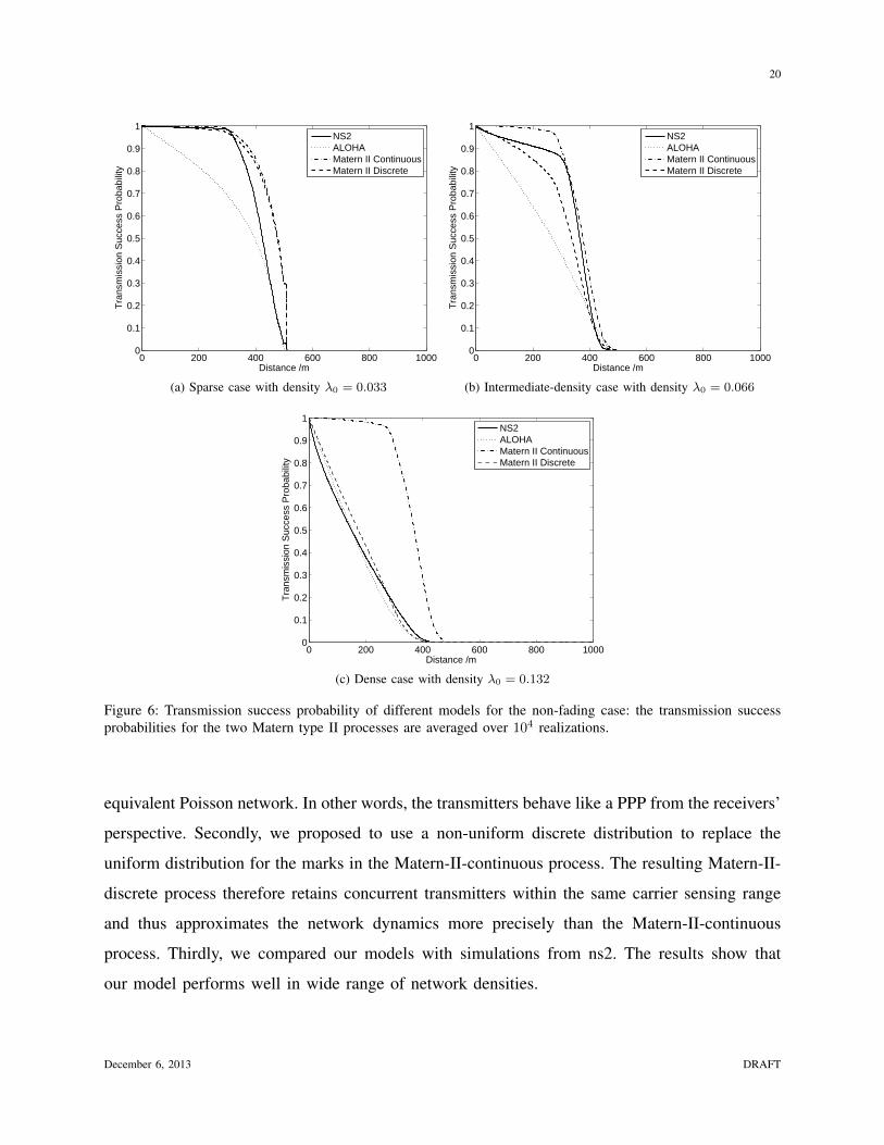
Fig. 6 shows the transmission success probabilities of the various models for the non-fading
case under different node densities λ0. Fig. 6(a) validates that the concurrent transmitters in
IEEE 802.11p form a hard-core process in the sparse case as discussed in Section III-B. For the
near distance (less than 300 m), the transmission success probability of the ns2 simulations is
December 6, 2013 DRAFT

19
very close to that of two Matern type II models. There is little difference between the Matern-II-
continuous and Matern-II-discrete processes since the probability that nodes within each other’s
carrier sensing range are transmitting simultaneously is zero in the sparse case.
For the intermediate-density case, Matern-II-discrete process produces a lower transmission
success probability than Matern-II-continuous process as it allows for nodes to have the same
marks. Although none of the three models can match ns2 simulations very well due to the
complexity of networks with intermediate densities, the Matern-II-discrete process provides the
closest approximation within 200 meters, which is the most critical range to vehicular safety.
In the dense case, the Matern-II-discrete process matches the ns2 simulation precisely. The
transmission success probability for ALOHA is also close to that of the ns2 simulation in the
dense case as claimed in [13] while it seems to be a very loose lower bound for the sparse and
intermediate cases. The transmission success probability for the Matern-II-continuous process
for the intermediate and dense cases look alike because there is saturation phenomenon in its
intensity λb, i.e., λb is upper bounded by λb,max = 12R
, where R is the carrier sensing range in
(4). For the non-fading case, R is fixed, and hence the maximum average number of retained
nodes on a road of length L from Matern-II-continuous process is upper bounded by L2R
, which
is independent of λ.
For the fading case, the performance of the Matern-II-discrete process shows the same trend
as in the non-fading case. However, ALOHA seems to have good performance as well. This can
be explained by the fact that fading randomizes the interference and therefore the actual network
is perceived as an equivalent Poisson network. A similar observation was made in [20] in the
case of cellular networks. In other words, fading dampens the hard-core effect and makes the
transmitter distribution look more like a PPP to the receivers. In addition, the lack of RTS/CTS
may further reduce the hard-core effect.
VI. CONCLUSIONS
In this paper, we explored the modeling of IEEE 802.11p for VANETs by using tools from
stochastic geometry and queueing theory. Firstly, we analyzed the distribution of transmitters for
networks with different densities. We found that without considering fading, by increasing the
network density, the transmitter distribution changes from a hard-core model to a Cox model.
With fading, the randomness of interference increases, which makes the networks appear as an
December 6, 2013 DRAFT
20
0 200 400 600 800 10000
0.1
0.2
0.3
0.4
0.5
0.6
0.7
0.8
0.9
1
Distance /m
Tra
nsm
issi
on S
ucce
ss P
roba
bilit
y
NS2ALOHAMatern II ContinuousMatern II Discrete
(a) Sparse case with density λ0 = 0.033
0 200 400 600 800 10000
0.1
0.2
0.3
0.4
0.5
0.6
0.7
0.8
0.9
1
Distance /m
Tra
nsm
issi
on S
ucce
ss P
roba
bilit
y
NS2ALOHAMatern II ContinuousMatern II Discrete
(b) Intermediate-density case with density λ0 = 0.066
0 200 400 600 800 10000
0.1
0.2
0.3
0.4
0.5
0.6
0.7
0.8
0.9
1
Distance /m
Tra
nsm
issi
on S
ucce
ss P
roba
bilit
y
NS2ALOHAMatern II ContinuousMatern II Discrete
(c) Dense case with density λ0 = 0.132
Figure 6: Transmission success probability of different models for the non-fading case: the transmission successprobabilities for the two Matern type II processes are averaged over 104 realizations.
equivalent Poisson network. In other words, the transmitters behave like a PPP from the receivers’
perspective. Secondly, we proposed to use a non-uniform discrete distribution to replace the
uniform distribution for the marks in the Matern-II-continuous process. The resulting Matern-II-
discrete process therefore retains concurrent transmitters within the same carrier sensing range
and thus approximates the network dynamics more precisely than the Matern-II-continuous
process. Thirdly, we compared our models with simulations from ns2. The results show that
our model performs well in wide range of network densities.
December 6, 2013 DRAFT

21
0 200 400 600 800 10000
0.1
0.2
0.3
0.4
0.5
0.6
0.7
0.8
0.9
1
Distance /m
Tra
nsm
issi
on S
ucce
ss P
roba
bilit
y
NS2ALOHAMatern II ContinuousMatern II Discrete
(a) Sparse case with density λ0 = 0.033
0 200 400 600 800 10000
0.1
0.2
0.3
0.4
0.5
0.6
0.7
0.8
0.9
1
Distance /m
Tra
nsm
issi
on S
ucce
ss P
roba
bilit
y
NS2ALOHAMatern II ContinuousMatern II Discrete
(b) Intermediate-density case with density λ0 = 0.066
0 200 400 600 800 10000
0.1
0.2
0.3
0.4
0.5
0.6
0.7
0.8
0.9
1
Distance /m
Tra
nsm
issi
on S
ucce
ss P
roba
bilit
y
NS2ALOHAMatern II ContinuousMatern II Discrete
(c) Dense case with density λ0 = 0.132
Figure 7: Transmission success probability of different models for the fading case: the transmission successprobabilities for the two Matern type II processes are averaged over 105 realizations.
REFERENCES
[1] IEEE standard for information technology-telecommunications and information exchange between systems-local and
metropolitan area networks-specific requirements; part 11: Wireless LAN medium access control (MAC) and physical
layer (PHY) specifications; amendment 6: Wireless access in vehicular environments, IEEE std. 802.11p. July 2010.
[2] Q. Chen, F. Schmidt-Eisenlohr, D. Jiang, M. Torrent-Moreno, L. Delgrossi, and H. Hartenstein. Overhaul of IEEE 802.11
modeling and simulation in ns-2. In the 10th International Symposium on Modeling Analysis and Simulation of Wireless
and Mobile Systems, MSWiM 2007, Chania, Crete Island, Greece, October 22–26, 2007, pages 159–168. ACM, 2007.
[3] M. Torrent-Moreno, J. Mittag, P. Santi, and H. Hartenstein. Vehicle-to-vehicle communication: Fair transmit power control
for safety-critical information. IEEE Transactions on Vehicular Technology, 58(7):3684–3703, Sept. 2009.
December 6, 2013 DRAFT

22
Parameter Valuecarrier frequency 5.9 GHz
packet size 414 Bytenoise floor −99 dBm
transmit power 10 dBmbroadcasting contention window (W + 1) 16
periodicity 100 msslot time δ 13µsmodulation BPSK
broadcast rate 6 Mbpspath loss exponent α 2path loss constant A −17.86 dBmreference distance r0 1
SINR threshold T 7 dBsimulation length L 10 km
Table II: Simulation Parameters
[4] G. Bianchi. Performance analysis of the IEEE 802.11 distributed coordination function. IEEE Journal on Selected Areas
in Communications, 18(3):535–547, March 2000.
[5] G. Bianchi, L. Fratta, and M. Oliveri. Performance evaluation and enhancement of the CSMA/CA MAC protocol for
802.11 wireless LANs. In Seventh IEEE International Symposium on Personal, Indoor and Mobile Radio Communications,
PIMRC’96, volume 2, pages 392–396, Oct 1996.
[6] F. Daneshgaran, M. Laddomada, F. Mesiti, and M. Mondin. Unsaturated throughput analysis of IEEE 802.11 in presence
of non ideal transmission channel and capture effects. IEEE Transactions on Wireless Communications, 7(4):1276–1286,
April 2008.
[7] Y.P. Fallah, C. L. Huang, R. SenGupta, and H. Krishnan. Analysis of information dissemination in vehicular ad-hoc
networks with application to cooperative vehicle safety systems. IEEE Transactions on Vehicular Technology, 60(1):233–
247, Jan. 2011.
[8] A. Tsertou and D.I. Laurenson. Revisiting the hidden terminal problem in a CSMA/CA wireless network. IEEE Transactions
on Mobile Computing, 7(7):817–831, July 2008.
[9] C. Han, M. Dianati, R. Tafazolli, R. Kernchen, and X. Shen. Analytical study of the IEEE 802.11p MAC sublayer in
vehicular networks. IEEE Transactions on Intelligent Transportation Systems, 13(2):873–886, 2012.
[10] Y. Yao, L. Rao, and X. Liu. Performance and reliability analysis of IEEE 802.11p safety communication in a highway
environment. IEEE Transactions on Vehicular Technology, 62(9):4198–4212, 2013.
[11] F. Baccelli and B. Blaszczyszyn. Stochastic Geometry and Wireless Networks, Volume II - Applications. Found. Trends
Netw., 2(1-2):1–312, 2009.
[12] M. Haenggi. Stochastic Geometry for Wireless Networks. Cambridge University Press, 2012.
[13] T. V. Nguyen, F. Baccelli, K. Zhu, S. Subramanian, and X. Z. Wu. A performance analysis of CSMA based broadcast
protocol in VANETs. In 2013 IEEE INFOCOM, pages 2805–2813, 2013.
[14] B. Błaszczyszyn, P. Muhlethaler, and Y. Toor. Maximizing throughput of linear Vehicular Ad-hoc NETworks (VANETs)
December 6, 2013 DRAFT

23
– a stochastic approach. In 2009 European Wireless Conference, pages 32–36, 2009.
[15] B. Błaszczyszyn, P. Muhlethaler, and Y. Toor. Stochastic analysis of Aloha in vehicular ad hoc networks. Annals of
Telecommunications, 68(1-2):95–106, 2013.
[16] D. H. Thuan, H. V. Cuu, and H. N. Do. VANET modelling and statistical properties of connectivity in urban environment.
REV Journal on Electronics and Communications, 3(1-2), January–June 2013.
[17] H.Q. Nguyen, F. Baccelli, and D. Kofman. A stochastic geometry analysis of dense IEEE 802.11 networks. In 2007 IEEE
INFOCOM, pages 1199–1207, May 2007.
[18] D.P. Bertsekas, R.G. Gallager, and P. Humblet. Data networks. Prentice-Hall International, 1992.
[19] G. Bansal, J.B. Kenney, and A. Weinfield. Cross-validation of DSRC radio testbed and ns-2 simulation platform for
vehicular safety communications. In 2011 IEEE Vehicular Technology Conference (VTC Fall), pages 1–5, 2011.
[20] B. Błaszczyszyn, M.K. Karray, and H.P. Keeler. Using Poisson processes to model lattice cellular networks. In 2013 IEEE
INFOCOM, pages 773–781, 2013.
December 6, 2013 DRAFT