1

Adaptive Data Fusion for Energy Efficient Routing

in Wireless Sensor Networks†

Hong Luo, Jun Luo, Yonghe Liu, and Sajal K. Das

{luo,juluo,yonghe,das}@cse.uta.edu

Dept. of Computer Science and Engineering

The University of Texas at Arlington, Arlington, TX 76019

Abstract

While in-network data fusion can reduce data redundancy and hence curtail network load, the fusion

process itself may introduce significant energy consumption for emerging wireless sensor networks with

vectorial data and/or security requirements. Through a set of experimental studies, we first demonstrate

that for certain applications, fusion costs indeed are comparable to those of communications. Therefore,

fusion-driven routing protocols for sensor networks cannot optimize over communication cost only –

fusion cost must also be accounted for. In our prior work [2], while a randomized algorithm termed

Minimum Fusion Steiner Tree (MFST)is devised towards this end, it assumes that datafusion shall be

performed at any intersection node whenever data streams encounter. Motivated by this limitation of

MFST, in this paper, we design a novel routing algorithm, calledAdaptive Fusion Steiner Tree (AFST),

for energy efficient data gathering in sensor networks. Not only does AFST jointly optimize over the

costs for both data transmission and data fusion, but also AFST evaluates the benefit and cost of data

fusion along information routes andadaptively adjusts whether fusion shall be performed at a particular

node. Analytically and experimentally, we show that AFST achieves better performance than existing

algorithms including SLT, SPT, and MFST.

Index Terms

sensor networks, data gathering, data fusion, routing

† A preliminary version of this work appeared in [1].

2

I. I NTRODUCTION

Wireless sensor networks have attracted a plethora of research efforts due to their vast potential

applications [3][4]. In particular, extensive research work has been devoted to providing energy

efficient routing algorithms for data gathering [5–19]. While some of these approaches assume

statistically independent information and have developed shortest path tree based routing strategies

[5, 6], others have considered the more realistic case of correlated data gathering [7–18]. By

exploring data correlation and employing in-network processing, redundancy among sensed data

can be curtailed and hence the network load can be reduced [8]. The objective of sensor routing

algorithms is then to jointly explore the data structure and network topology to provide the optimal

strategy for data gathering with as minimum energy as possible.

Regardless of the techniques employed, existing strategies miss one key dimension in the

optimization space for routing correlated data, namely thedata aggregation cost. Indeed, the cost

for data aggregation may not be negligible for certain applications. For example, sensor networks

monitoring field temperature may use simple average, max, or min functions which essentially are

of insignificant cost. However, other networks may require complex operations for data fusion1.

Energy consumption of beamforming algorithm for acoustic signal fusion has been shown to be

on the same order of that for data transmission [20]. Moreover, encryption and decryption at

intermediate nodes will significantly increase fusion cost in the hop-by-hop secure network since

the computational cost is on the scale ofnJ per bit [21]. In our own experimental study described

in the Appendix, we show that aggregation processes such as image fusion cost tens ofnJ per

bit, which is on the same order as the communication cost reported in the literature [7, 20].

Different from transmission cost that depends on the output of the fusion function, the fusion cost

is mainly determined by the inputs of the fusion function. Therefore, in addition to transmission

1In this paper we will consider “aggregation” and “fusion” interchangeable, denoting the data reduction process on intermediatesensor nodes.

3

cost, the fusion cost can significantly affect routing decisions when involving data aggregation.

In our prior work [2], we presented a randomized algorithm termedMinimum Fusion Steiner

Tree (MFST)that jointly optimizes over both the fusion and transmission costs to minimize

overall energy consumption. MFST is proved to achieve a routing tree that exhibits54log(n + 1)

approximation ratio to the optimal solution, wheren denotes the number of source nodes.

While MFST has been shown to outperform other routing algorithms includingShortest Path

Tree (SPT), Minimum Spanning Tree(MST), andShallow Light Tree(SLT) in various system

settings, it assumes that aggregation is performed at the intersection nodeswheneverdata streams

encounter. However, as we shall show below, such a strategy may introduce unnecessary energy

consumption. Specifically, performing fusion at certain nodes may be less efficient than simply

relaying the data directly. This observation motivates us to design an adaptive fusion strategy that

not only optimizes information routes, but also embeds the decisions as to when and where fusion

shall be performed in order to minimize the total network energy consumption.

A. Motivation

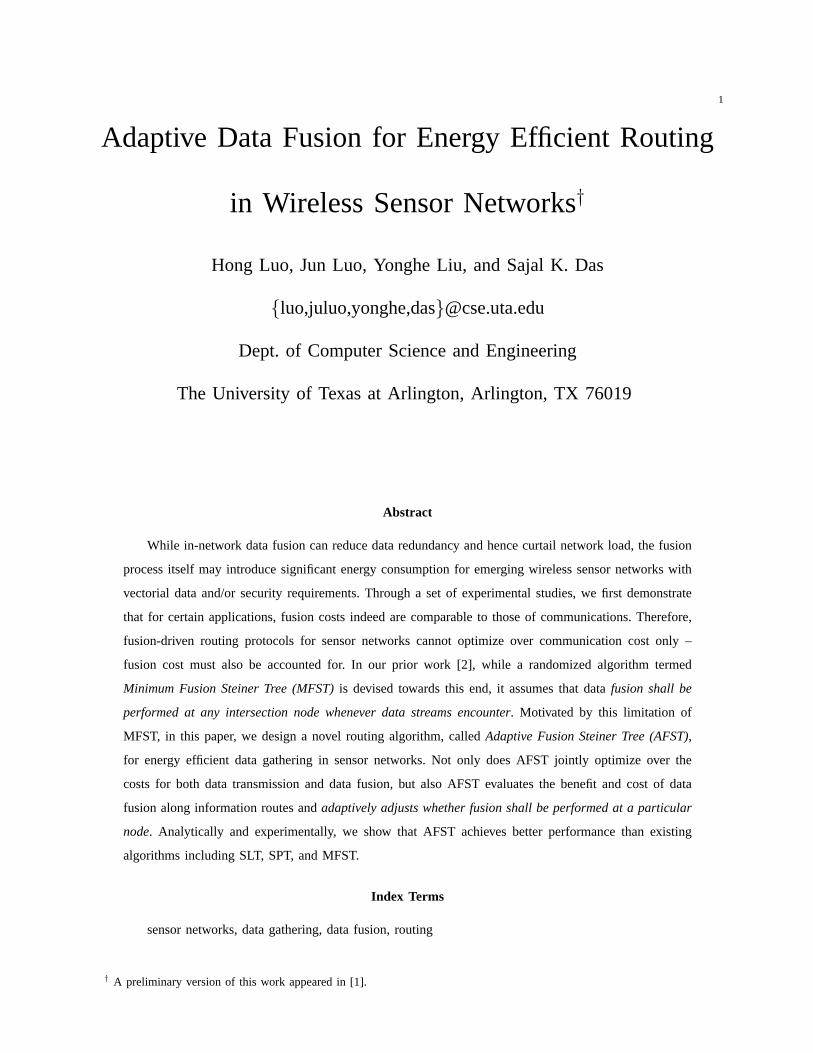
Fig. 1 depicts a sensor network where sensor nodessource

router

sink

fusion point

L h

o p s

v

s

u

t

A B

Fig. 1. Illustration of fusion benefit, or disadvantage,

in sensor networks.

are deployed on grid and sensed information of the

source nodes is to be routed to sinkt. Arrow lines form

the aggregation tree in which nodesu and v initially

aggregate data of areasA andB, respectively. As the

sink is far away,u and v further aggregate their data

at v and then send one fused data to the sink. Assume

each hop has identical unit transmission costc0, the fusion cost is linear to the total amount of

incoming data, and the unit fusion cost isq0. Let w(u) andw(v) respectively denote the amount of

data atu andv before the aggregation between them. The amount of resultant aggregated data atv

4

can be expressed as(w(u)+w(v))(1−σuv), whereσuv represents the data reduction ratio owing to

aggregation. In this scenario, ifv performs data fusion, the total energy consumption of the route

from v to t, assuming there areL hops in between, isLc0(w(u)+w(v))(1−σuv)+q0(w(u)+w(v)).

On the contrary, ifv does not perform data fusion, the total energy consumption of the same route

is simply the total relaying cost,Lc0(w(u) + w(v)). To minimize thetotal energy consumption of

the network, v should not perform data fusion as long asσuv < q0

Lc0.

This simple example reveals that to minimize total network energy consumption, the decision at

an individual node has to be based on data reduction ratio due to aggregation, its related cost, and

its effect on the communication costs at the succeeding nodes. Although the criteria can be easily

obtained for this simple example, a sensor network confronting various aggregation/communication

costs, and data/topology structures, undoubtedly will dramatically augment the difficulty of the

fusion decisions.

B. Our Contribution

In this paper, we proposeAdaptive Fusion Steiner Tree(AFST), a routing scheme that not

only optimizes over both transmission and fusion costs, but also adaptively adjusts its fusion

decisions for sensor nodes. By evaluating whether fusion is beneficial to the network based on

fusion/transmission costs and network/data structures, AFST dynamically assigns fusion decisions

to routing nodes during the route construction process. Analytically we prove that AFST out-

performs MFST. Through an extensive set of simulations, we demonstrate that AFST provides

significant energy saving over MFST (up to 70%) and other routing algorithms under a wide

range of system setups. By adapting both the routing tree and fusion decisions to various network

conditions, including fusion cost, transmission cost, and data structure, AFST provides a routing

algorithm suitable for a broad range of applications.

In particular, we prove that the routing tree resulted from AFST consists of two parts: a lower

part where aggregation is always performed, and an upper part where no aggregation occurs. The

5

result can be readily applied in designing clustering algorithms in sensor networks: based on where

fusion stops, the network can be partitioned into clusters where data aggregation is confined to

be within the clusters only.

The remainder of this paper is organized as follows. In Section II, we describe the system

model and formulate the routing problem. Section III first gives an overview of the randomized

approximation algorithm MFST, and then presents in detail the design and analysis of the proposed

algorithm AFST. In section IV we experimentally study the performance of AFST. Section V gives

the related work and section VI concludes the paper.

II. SYSTEM MODEL AND PROBLEM FORMULATION

A. Network Model

We model a sensor network as a graphG = (V, E) whereV denotes the node set andE the

edge set representing the communication links between node-pairs. We assume a setS ⊂ V of n

nodes, are data sources of interests and the sensed data needs to be sent to a special sink node

t ∈ V periodically. We refer the period of data gathering as around in this paper.

For a nodev ∈ S, we define node weightw(v) to denote the amount of information outgoing

from v in every round. An edgee ∈ E is denoted bye = (u, v), whereu is the start node andv is

the end node. The weight of edgee is equivalent to the weight of its start node, i.e.,w(e) = w(u).

Two metrics,t(e) andf(e), are associated with each edge, describing the transmission cost and

fusion cost on the edge, respectively.

Transmission cost,t(e), denotes the cost for transmittingw(e) amount of data fromu to v. we

abstract the unit cost of the link for transmitting data fromu to v asc(e) and thus the transmission

cost t(e) is

t(e) = w(e)c(e). (1)

6

Notice thatc(e) is edge-dependent and hence can accommodate various conditions per link, for

example, different distances between nodes and local congestion situations.

Fusion cost,f(e) denotes energy consumption for fusion process at theend node v. f(e)

depends on the amount of data to be fused as well as the algorithms utilized. In this paper, we

useq(e) to abstract the unit fusion cost on edgee. Since data fusion is performed by intermediate

nodes to aggregate their own data with their children’s, in order to avoid confusion, we usew(·)

to denote the temporary weight of a nodebefore current data fusion. Then the cost for fusing the

data of nodesu andv at nodev is given by

f(e) = q(e) ·(w(u) + w(v)

). (2)

Key to a sensor data routing protocol with data fusion is the data aggregation ratio. Unfortu-

nately, this ratio is heavily dependent on application scenarios. Here, we use an abstract parameter

σ to denote the data reduction ratio due to aggregation. To be more specific, if nodev is responsible

for fusing nodeu’s data (denoted byw(u)) with its own, we havew(v) = (w(u)+w(v))(1−σuv),

wherew(v) andw(v) denotes the data amount of nodev before and after fusion. Notice thatσu,v

may be different before and after the fusion process between nodeu and another node, as the

weight w(u) will change by the fusion and the data correlation between nodeu and v will be

different as well.

Due to aggregation cost, nodev may choose not to perform data aggregation in order to realize

maximum energy saving. Instead, it will simply relay the incoming data of nodeu. In this case, the

new weight of nodev is simply w(v) = (w(u) + w(v)). Jointly considering both cases described

above, we can summarize the aggregation function at nodev as

w(v) = (w(u) + w(v))(1− σuvxuv), (3)

wherexuv ∈ {0, 1} denotes whether fusion occurs on edgee = (u, v).

7

B. Problem Formulation

Given the source node setS and sinkt, our objective is to design a routing algorithm that

minimizes the energy consumption when delivering data from all source nodes inS to the sinkt.

Not only do we need to design routing paths back hauling sensed information driven by information

aggregation, but also we have to optimize over the decisions as to whether aggregation shall occur

or not on a particular node.

Mathematically, a feasible routing scheme is a connected subgraphG′ = (V ′, E ′) whereG′ ⊂ G

contains all sources (S ⊂ V ′) and the sink (t ∈ V ′). Depending on whether fusion is performed

or not, the edge setE ′ can be divided into two disjoint subsetsE ′f andE ′

n, whereE ′f = {e|e ∈

E ′, xe = 1} andE ′n = {e|e ∈ E ′, xe = 0}. Our goal is to find a feasible subgraphG∗ such that

G∗ = argminG′∑

e∈E′f

(f(e) + t(e)

)+

∑

e∈E′n

t(e) (4)

III. D ESIGN AND ANALYSIS OF AFST

While MFST [2] has provided an approximation routing algorithm that jointly optimizes over

both the transmission and fusion costs with proven performance bound, it lacks fusion decisions

in routing construction. This motivates us to designAdaptive Fusion Steiner Tree (AFST), which

achieves significantly better performance than MFST due to the incorporation of fusion decision.

In designing AFST to solve the optimization problem as presented in (4), our approach is as

follows. By exploiting certain network properties, we first propose a heuristic solution termed

Binary Fusion Steiner Tree(BFST), which is analytically shown to have better performance than

MFST. However, BFST is still constrained to the tree structure obtained from MFST. By employing

SPT rather than the structure obtained via MFST, where appropriate, we further improve BFST

to AFST. As a result, we are able to analytically show that AFST is capable of achieving better

performance than BFST.

As AFST is based on MFST, we first give a brief overview of MFST. Then we introduce fusion

8

decisions into the routing structure generated by the MFST scheme. Following that, we detail our

new solution.

A. Brief Overview of MFST

The minimum fusion steiner tree (MFST) is based on the techniques presented in [14, 22]. It

first pairs up source nodes (or source with the sink) based on defined metrics and then randomly

selects a center node from the node-pair. The weight of the non-center node will be transferred to

the center node, paying appropriate transmission and fusion costs on that edge. Subsequently, the

non-center node will be eliminated and the center node with aggregated weight will be grouped

as a new set of sources. This process will then be repeated on the new set until the sink is the

only remaining node. The algorithm is detailed below for the sake of completeness.

MFST ALGORITHM:

1) Initialize the loop indexi = 0. DefineS0 = S ∪ {t}, andE∗ = ∅. Let w0(v) for any v ∈ S

denote its original weight, and letw0(t) = 0.

2) For every pair of nodes(u, v) ∈ Si:

• Find the minimum cost path(u, v) in G according to the metric

M(e) = q(e) · (wi(u) + wi(v)) + α(wi(u), wi(v))c(e) (5)

whereα(wi(u), wi(v)) = wi(u)wi(v)(wi(u)+wi(v))

w2i (u)+w2

i (v)if (u, v) is no-sink pair andα(wi(u), wi(v)) =

wi(u) if v is just the sinkt.

• DefineKi(u, v) to be the distance under metricM(e) of this path.

3) Find minimum-cost perfect matching2 between nodes inSi. Let (ui,j, vi,j) denote thej-th

matched pair inSi, where1 ≤ j ≤ |Si|/2. If there is only one non-sink node left after

matching, match it to itself without any cost, and consider it as the last “single-node pair”

2Minimum-cost perfect matching is a matching of edges in a graph that guarantees the total cost (distance) for all pairs underM(e) is minimized. For polynomial-time algorithms for this problem, see [23].

9

in Si.

4) For each matched pair(u, v), add those edges that are on the path definingKi(u, v) to set

E∗.

5) For each pair of non-sink matched nodes(u, v), chooseu to be the center with probability

P (u = center) =w2

i (u)

w2i (u)+w2

i (v). Otherwise, nodev will be the center. For pair(u, t), choose

sink t to be the center.

6) Transport weight of non-center node to its corresponding center node. The weight of the

center satisfieswi+1(center) = (wi(u) + wi(v))(1− σuv).

7) Remove all non-center nodes fromSi, then the remaining center nodes induceSi+1.

8) If Si+1 contains only the sink, we returnG∗ = (V ∗, E∗), whereE∗ is the set of edges

we constructed andV ∗ includes the source nodes and the sink. Otherwise incrementi and

return to step 2.

In MFST, the size of the setSi is reduced half after one iteration of the algorithm. Therefore,

the process terminates afterlog(n + 1) iterations. In the remainder of this paper, we call each

iteration a “stage” of the algorithm.

MFST jointly considers both fusion and transmission costs. It has been shown that it yields

54log(n+1) approximation ratio to the optimal solution. Although extensive experiments [2] have

shown that MFST can outperform other routing algorithms including SLT, SPT, and MST, one

optimizing dimension is still missing, namely the aforementioned fusion decisions at sensor nodes.

As MFST requires fusion to be performed along a routing path whenever possible, unnecessary

energy may be wasted due to the inefficiency of fusion, for example, little information reduction

due to weak correlation and high fusion cost.

Specially, this phenomena can be magnified in the proximity of the sink itself. As aggregated

information streams are approaching the sink, their correlation decreases which will introduce

10

small data reduction owing to fusion. At the same time, directly relaying the data will not incur

high communication cost as fewer hops are needed for relaying. Naturally, in this scenario, there

is a high probability for direct relaying to outperform aggregation.

To solve this problem, we design AFST where adaptive fusion decisions will be incorporated

into the routing construction process.

B. 3-D Binary Tree Structure

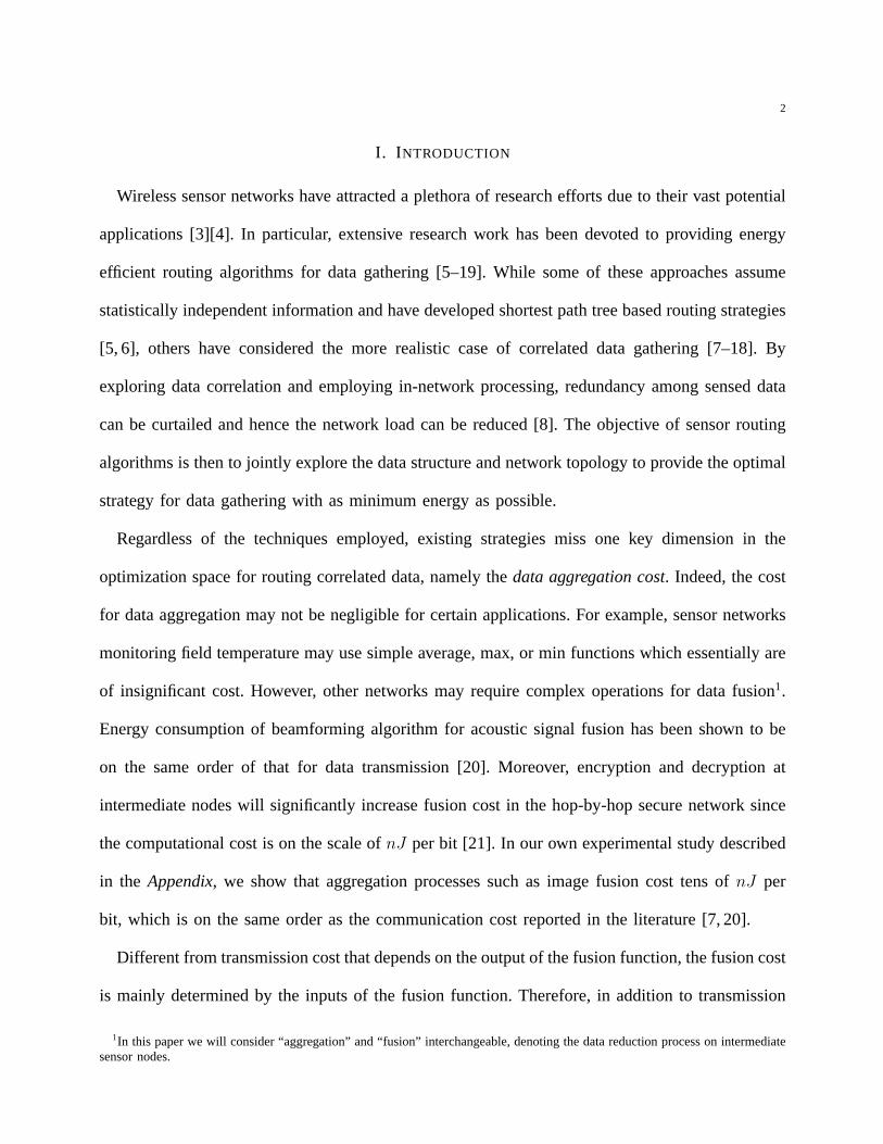
In order to make our analysis more clear, we use a 3-D binary tree structure to describe the

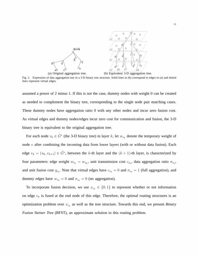
process of the hierarchical matching technique used in MFST. Fig. 2 illustrates a mapping example

of original aggregation tree and its transformation. From bottom to top, the edges between two

layers represent the result of node matching and center selection in each iteration of MFST.

Assuming there aren sources in the aggregation treeG∗ obtained via MFST, to perform the

transformation, we first cloneN = dlog(n + 1)e copies ofG∗, denoted byG1, G2, . . . , GN . For

convenience, we label the originalG∗ as G0 and arrange them into vertical layers as shown in

Fig. 2(b). For simplification, we will refer nodev’s clone in layerk asvk. Subsequently, we map

the original aggregation treeG∗ as shown in Fig. 2(a) to a new graphG∗ embedded into these

clones.G∗ is the targeted 3-D binary tree. The process is to map the result of each matching stage

k in MFST to the edges betweenGk andGk+1. If we matchu andv in stagek andv is selected

as the center node in MFST, we first add an edgee linking v’s clones inGk andGk+1 with zero

unit transmission costc(e) = 0. This edge is termed virtual edge (dotted line). Then we connect

uk to vk+1 with the same unit communication costc(e) as inG∗.

The result of this transformation is a binary tree which is rooted at the sink inGN and has all

leaves inS residing inG0. For each sourcev ∈ S, there is a path going through all clones ofG∗,

from v in G0 to the sinkt in GN , via exactlyN hops.

In order to guarantee that the resulting 3-D tree is binary, the number of source nodes is

11

a

t ( sink )

g f

e

d

c

b

(a) Original aggregation tree.a

t g f

e d

c b

t f d b

G 0

G 1

t d

G 2

t

G 3

(b) Equivalent 3-D aggregation tree.Fig. 2. Expression of data aggregation tree in a 3-D binary tree structure. Solid lines in (b) correspond to edges in (a) and dottedlines represent virtual edges.

assumed a power of 2 minus 1. If this is not the case, dummy nodes with weight 0 can be created

as needed to complement the binary tree, corresponding to the single node pair matching cases.

These dummy nodes have aggregation ratio 0 with any other nodes and incur zero fusion cost.

As virtual edges and dummy nodes/edges incur zero cost for communication and fusion, the 3-D

binary tree is equivalent to the original aggregation tree.

For each nodevk ∈ G∗ (the 3-D binary tree) in layerk, let wvkdenote the temporary weight of

nodev after combining the incoming data from lower layers (with or without data fusion). Each

edgeek = (uk, vk+1) ∈ G∗, between thek-th layer and the(k + 1)-th layer, is characterized by

four parameters: edge weightwek= wuk

, unit transmission costcek, data aggregation ratioσek

,

and unit fusion costqek. Note that virtual edges havecek

= 0 andσek= 1 (full aggregation), and

dummy edges havewek= 0 andσek

= 0 (no aggregation).

To incorporate fusion decision, we usexek∈ {0, 1} to represent whether or not information

on edgeek is fused at the end node of this edge. Therefore, the optimal routing structures is an

optimization problem overxekas well as the tree structure. Towards this end, we presentBinary

Fusion Steiner Tree(BFST), an approximate solution to this routing problem.

12

C. Binary Fusion Steiner Tree (BFST)

In BFST, we first obtain a routing tree using MFST algorithm, where fusion is performed by

any intermediate node. Subsequently, we evaluate whether fusion on individual nodes will reduce

the energy consumption of the network. If not, the fusion process on the node will be cancelled

and instead data will be directly relayed.

BFST ALGORITHM:

1) Run MFST algorithm to obtain routing tree with fusion at every node possible. Convert the

resulting aggregation tree to the 3-D binary tree as described above. For all edges in the

tree, setxek= 1.

2) From bottom to top, calculate the fusion benefit for each edge in the aggregation tree

(excluding virtual edges), which can represent the energy saving by data fusion on that

edge. Let∆uk,vk+1denote the fusion benefit of edgeek = (uk, vk+1). It is defined as

∆uk,vk+1= (wuk

+ wvk)C(vk+1, tN)−

((wuk

+ wvk)(1− σek

)C(vk+1, tN) + qek(wuk

+ wvk))

(6)

whereC(vk+1, tN) denotes the summation of unit transmission costs fromvk+1 to tN in

MFST. Setxek= 1 if ∆uk,vk+1

> 0; otherwise, setxek= 0.

3) For all edges withxuk,vk+1= 0, setxvk,vk+1

= 0 to their corresponding virtual edges.

In our analysis, we will employ the 3-D binary tree described in the previous subsection. To

simplify the analysis, we assume that in BFST, the data reduction ratioσ is non-increasing on

each path from the source to the sink while the unit fusion costq is non-decreasing, excluding

virtual edges. This assumption can be naturally justified. First, strong correlation and thus high

aggregation ratio usually are due to spatial correlation resulting from short distances between

nodes. In turn, these short distances will lead to small unit transmission cost. Based on the metric

M(e) defined in MFST (which is a combination of fusion cost and transmission cost), it will

match strongly correlated nodes before matching weakly correlated nodes. Therefore, for edges

13

on a source-sink path, the aggregation ratio for edges near the sink will not be larger than those

further away. Reflected on the 3-D binary tree, this will lead to non-increasingσ on a particular

source-sink path. The reason for skipping virtual edges is that their data aggregation ratio is set

to 1 and does not affect the actual energy consumption of the network. Second, the unit fusion

cost q is determined mainly by the complexity of the fusion algorithm and the input data set.

As the information is being routed toward the sink, the data size and complexity will naturally

increase due to aggregation on the route. Therefore, performing fusion thereon will incur more

computation and hence more energy consumption per unit data.

Based on this assumption, we first introduce Lemma 1.

Lemma 1:xe is non-increasing on each path from a source to the sink in BFST.

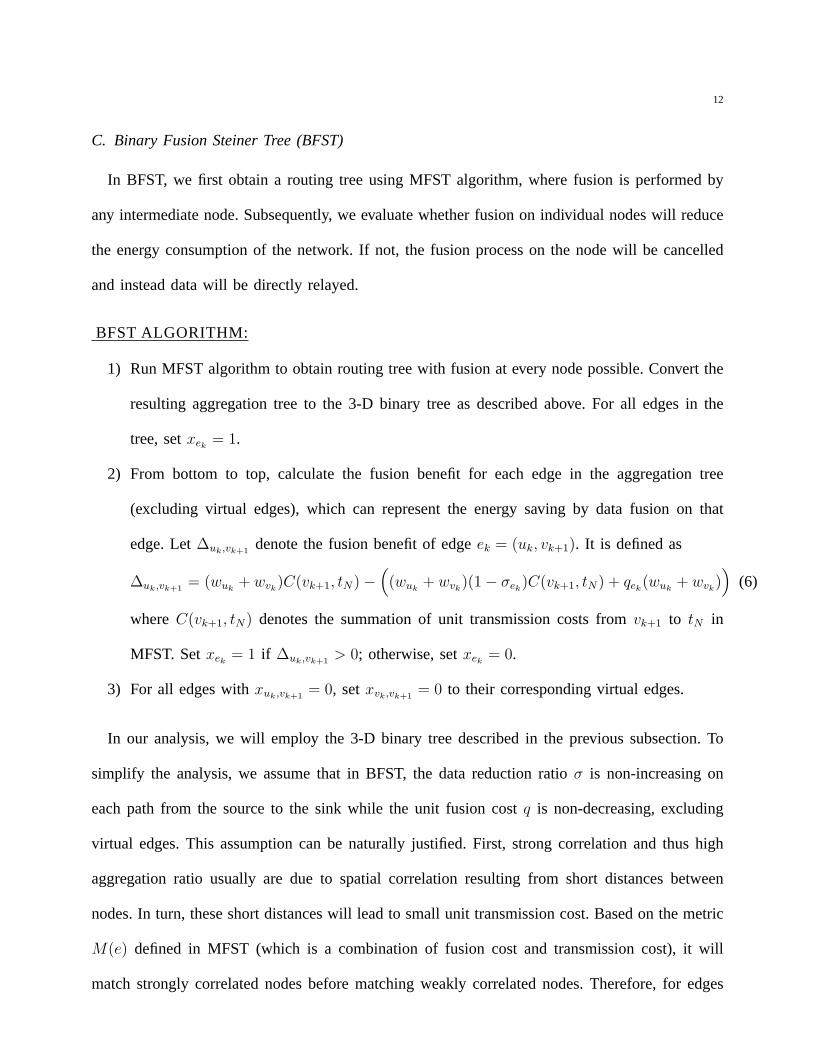
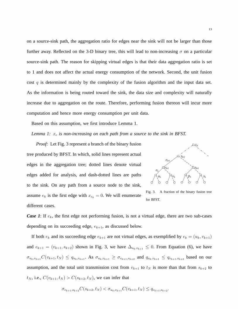
Proof: Let Fig. 3 represent a branch of the binary fusion

u k v k

v k + 1

p k s k

s k + 1

s k + 2

t N

e k + 1

e k

Fig. 3. A fraction of the binary fusion tree

for BFST.

tree produced by BFST. In which, solid lines represent actual

edges in the aggregation tree; dotted lines denote virtual

edges added for analysis, and dash-dotted lines are paths

to the sink. On any path from a source node to the sink,

assumeek is the first edge withxek= 0. We will enumerate

different cases.

Case 1: If ek, the first edge not performing fusion, is not a virtual edge, there are two sub-cases

depending on its succeeding edge,ek+1, as discussed below.

If both ek and its succeeding edgeek+1 are not virtual edges, as exemplified byek = (uk, vk+1)

and ek+1 = (vk+1, sk+2) shown in Fig. 3, we have∆uk,vk+1≤ 0. From Equation (6), we have

σuk,vk+1C(vk+1, tN) ≤ quk,vk+1

. As σuk,vk+1≥ σvk+1,sk+2

and quk,vk+1≤ qvk+1,sk+2

based on our

assumption, and the total unit transmission cost fromvk+1 to tN is more than that fromsk+2 to

tN , i.e., C(vk+1, tN) > C(sk+2, tN), we can infer that

σvk+1,sk+2C(sk+2, tN) < σuk,vk+1

C(vk+1, tN) ≤ qvk+1,sk+2.

14

This will lead to∆vk+1,sk+2< 0. Consequently, we havexvk+1,sk+2

= 0.

If ek is not a virtual edge but its succeeding edgeek+1 is, as exemplified byek = (pk, sk+1)

andek+1 = (sk+1, sk+2), the same conclusion can be obtained similarly.

Case 2:If ek is a virtual edge, as exemplified byek = (vk, vk+1), according to BFST algorithm,

its matching pair edgee′k = (uk, vk+1) must havexuk,vk+1= 0. From the result of Case 1, we also

havexvk+1,sk+2= 0.

Inductively, we can conclude that all succeeding edges of an edge that does not perform fusion

will not perform fusion either. Since the fusion decisionxek∈ {0, 1}, it is evident thatxe is

non-increasing on the path from source to sink.

Theorem 1:The total cost of BFST is no more than MFST.

Proof: Since BFST retains the same tree structure as MFST, for all edges withxek= 1, the

BFST and MFST schemes will consume the same amount of energy. For any edge withxek= 0,

owing to Lemma 1, any edgeei on the path from this edge to the sink satisfyxei= 0. This

means that all edges on the path afterek have negative effect on energy conservation. In other

words, performing fusion will introduce additional cost. Therefore, BFST is a better algorithm

than MFST by avoiding fusion when direct relaying is a better choice.

Intuitively, Lemma 1 depicts that the routing tree generated by BFST can be divided into two

parts: the lower part where data aggregation is always performed and the upper part where direct

relaying is employed. As no data aggregation is performed in the upper part of the tree, instead

of sticking to MFST, we can further improve the routing structure to reduce energy consumption.

Inspired thereby, we develop AFST.

D. Adaptive Fusion Steiner Tree (AFST)

AFST further improves BFST by introducing SPT into the routing tree. Similar to BFST, it

performs a matching process as in MFST in order to jointly optimize over both transmission

15

and fusion costs. During the matching process, it also dynamically evaluates if fusion shall be

performed or not. If it is determined at a particular point that fusion is not beneficial to the

network, as shown by the analysis of BFST, we can conclude that any succeeding nodes on the

routing path shall not perform fusion either. Consequently, we can employ SPT as the strategy

for the remainder of the route as SPT is optimal for routing information without aggregation. Our

analysis shows that AFST achieves better performance than BFST and thereon MFST.

AFST ALGORITHM:

1) Initialize the loop indexi = 0. DefineS0 = S ∪ {t}, andE∗ = ∅. Let wv0 for any v ∈ S

equal to its original weight, and letwt0 = 0.

2) For every pair of non-sink nodes(u, v) ∈ Si: find the minimum cost path(u, v) in G

according to the metric

M(e) = qui,vi+1(wui

+ wvi) + α(wui

, wvi)c(e). (7)

DefineKi(u, v) to be the distance under metricM(e) of this path.

3) Find minimum-cost perfect matching between nodes inSi. If there is only one non-sink

node left after matching, match it to itself without any cost, and consider it as the last

“single-node pair” inSi.

4) For each matched pair(u, v), calculate the fusion benefit for nodeu and v respectively

according to this new definition:

∆ui,vi+1= (wui

+ wvi)SP (vi, t)−

((wui

+ wvi)(1− σei

)SP (vi, t) + qei(wui

+ wvi)), (8)

whereSP (vi, t) denotes the summation of unit transmission cost fromvi to the sinkt using

shortest path.

We call(u, v) a non-fusion pair if there is no fusion benefit regardless which node is selected

as the center. It means that the two following inequations are satisfied

∆ui,vi+1< 0 and ∆vi,ui+1

< 0. (9)

16

Otherwise, we call them a fusion pair.

5) For each non-fusion pair(u, v),

• Add those edges that are on the shortest paths of(u, t) and (v, t) to setE∗n.

• Remove both nodesu andv from Si.

6) For each fusion pair(u, v),

• Add those edges that are on the path definingKi(u, v) to setE∗f .

• chooseu to be the center with probabilityP (u = center) =w2

ui

w2ui

+w2vi

. Otherwisev will

be the center. For pair(u, t), choose sinkt to be the center.

• Transport weight of non-center node to its corresponding center node. According to

Equation (3), the weight of the center satisfieswi+1(center) = (wui+wvi

)(1−σui,vi+1).

• Remove all non-center nodes fromSi, then the remaining center nodes induceSi+1.

7) If Si+1 is empty or contains only the sink, we returnG∗ = (V ∗, E∗) (E∗ = E∗f + E∗

n),

where E∗f and E∗

n is the set of fusion edges and non-fusion edges, respectively, andV ∗

includes source nodes and the sink. Otherwise, incrementi and return to step 2.

The size of setSi is reduced at least half after one run of the algorithm. However, the process

may terminate sooner than MFST and BFST if fusion is deemed unworthy in the early iterations.

Theorem 2:The total cost of AFST is no more than BFST.

Proof: The tree resulting from AFST also contains a lower part where aggregation is always

performed and an upper part where no aggregation occurs. The lower part of AFST is the same

as that of BFST due to their MFST based matching procedure and thus incurs the same cost as

well. The task left is then to show that for any non-fusion pair(u, v) satisfying inequality (9),

their transmission costs based on SPT in AFST is no more than the corresponding routing costs,

including fusion and transmission costs, incurred in BFST. The proof is given below.

From (9), we haveσuk,vk+1SP (vk, t) < quk,vk+1

andσvk,uk+1SP (uk, t) < qvk,uk+1

whereSP (vk, t)

17

denotes the summation of unit transmission cost fromvk to the sinkt using shortest path. Without

loss of generality, assume thatv is selected as the center in BFST, and our goal is to prove

wvkSP (vk, t) + wuk

SP (uk, t) < wukc(uk, vk+1) + quk,vk+1

(wuk+ wvk

) (10)

+(wuk+ wvk

)(1− σuk,vk+1)SP (vk+1, t).

For that, we have

wvkSP (vk, t) + wuk

SP (uk, t)

≤ wvkSP (vk+1, t) + wuk

(c(uk, vk+1) + SP (vk+1, t))

= (wuk+ wvk

)SP (vk+1, t) + wukc(uk, vk+1)

= (wuk+ wvk

)(1− σuk,vk+1+ σuk,vk+1

)SP (vk+1, t) + wukc(uk, vk+1)

≤ (wuk+ wvk

)(1− σuk,vk+1)SP (vk+1, t) + quk,vk+1

(wuk+ wvk

) + wukc(uk, vk+1)

When it is determined that the fusion benefit is positive for every node, the tree structure

obtained from AFST degenerates to the tree from MFST. However, when fusion is not always

beneficial for all nodes, AFST will stop doing nonsensical data fusion and directly deliver data

to the sink for more energy saving, as a result, it can significantly outperform MFST. From the

process of route construction, we can see that AFST can dynamically assign fusion decisions to

routing nodes during the route construction process by evaluating whether fusion is beneficial to

the network based on fusion/transmission costs and network/data structures.

E. Application in Clustering

Clustering in sensor networks is often used to group closely correlated sensor together in order

to perform local decision making, detection, or classification. To facilitate these operations, fusion

and transmission cost shall be considered due to severe resource constraints. While the concept

of clustering has been widely applied, clustering itself is often based on static techniques mainly

18

based on geographic proximity, fixed cluster number, or certain cluster sizes.

The two-layer structure of AFST naturally provides a new clustering technique for sensor

networks. Separated by the routing nodes not performing fusion, the lower part of AFST routing

tree is composed of discrete branches within which data of every member will be fused together.

These branches can be considered as clusters decided by energy consumption due to fusion and

communication. Therefore, AFST provides a clustering algorithm as a byproduct that is energy

efficient for gathering correlated data. Sensors in the same cluster will employ MFST based routing

structure while cluster heads (roots of the branches) will directly send the aggregated data to the

sink via shortest path without fusion. Since AFST is a randomized algorithm, we can rerun the

process to generate a different structure and therefore re-assign the role of cluster heads to different

nodes. Load balancing in terms of fusion is thus naturally implemented.

IV. EXPERIMENTAL STUDY

In this section, we compare the performance of AFST with other routing algorithms. In partic-

ular, we select MFST, SPT, MST, and SLT to represent the class of routing schemes where fusion

occurs on all routing nodes if possible. For routing schemes that does not perform aggregation,

we employ SPT as it is the optimal routing strategy in this class. To distinguish it from the SPT

scheme with data aggregation opportunistically occurs where information streams intersect, we

denote the SPT without performing aggregation by SPT-nf, short name for SPT-no-fusion.

We study the impact of network connectivity, correlation coefficient, and unit fusion cost on

different algorithms. Concurring with our design goal and analysis of the AFST algorithm, our

key finding of the experiments is that AFST can adapt itself to a wide range of data correlations

and fusion cost. Therefore, AFST can achieve better performance in all kinds of system setups.

19

A. Simulation Environment

In our setup, 100 sensor nodes are uniformly distributed in a region of a50m × 50m square.

We assume that each node produces one 400-byte packet as original sensed data in each round

and sends the data to the sink located at the bottom-right corner. All sensors act as both sources

and routers. We also did sets of experiments of different number of sensors and different sizes of

field, the results are similar and omitted here.

We assume the maximal communication radius of a sensor isrc, i.e, if and only if two sensor

nodes are withinrc, there exists a communication link between them, or an edge in graphG. By

varying rc, we can control the network connectivity and hence equivalently the network density.

We instantiate unit transmission cost on each edge,c(e), using the first order radio model presented

in [7]. According to this model, the transmission cost for sending one bit from one node to another

that isd distance away is given byβdγ + ε whend < rc, whereγ andβ are tunable parameters

based on the radio propagation. We setγ = 2 and β = 100pJ/bit/m2 to calculate the energy

consumption on the transmit amplifier.ε denotes energy consumption per bit on the transmitter

circuit and receiver circuit. Typical values ofε range from20 to 200nJ/bit according to [20]. We

set it to be100nJ/bit in our simulation.

We model data reduction due to aggregation based on correlation among sensed data. The

correlation model employed here is an approximated spatial model where the correlation coefficient

(denoted byρ) decreases with the distance between two nodes provided that they are within the

correlation range,rs. If two nodes are more thanrs distance apart, simply the correlation coefficient

ρ = 0. Otherwise, it is given byρ = 1− d/rs, whered denotes the distance between the nodes.

If node v is responsible for fusing nodeu’s data (denoted byw(u)) with its own, we assume that

the weight of nodev after fusion is given by

w(v) = max(w(u), w(v)) + min(w(u), w(v))(1− ρuv)

20

wherew(v) andw(v) respectively denote the data amount of nodev beforeandafter fusion.

Recall that we useσ to denote the data reduction ratio due to aggregation. From Equation (3),

w(v) = (w(u)+w(v))(1−σuv) if fusion is performed at nodev, we can get that the data reduction

ratio σuv is proportional to the correlation coefficientρ. By varying the correlation rangers, we

can control the average correlation coefficient of the network, and further control the average data

reduction after data fusion. For example, a very smallrs essentially eliminates the correlation

among sensors (ρ → 0), so that the amount of output data is equal to the summation of all input

data. While an extremely largers makes the sensed data completely redundant (ρ → 1), as a result,

the fused data size equals to the bigger data size between the two input data. In our simulation,

we useρ instead ofσ to describe the impact of data structure for ease of understanding. For the

fusion cost, we assume thatq is constant and useω to denote the average fusion cost per bit at

each node.

In the following subsections, we will study the performance of AFST and other algorithms

under various system setups, including network connectivity, correlation coefficient, and fusion

cost.

B. Impact of Network Connectivity

Since rc denotes the communication range of a node, by varyingrc, we can control the

connectivity of the network. Here we setω, the average unit fusion cost, to be80nJ/bit, which

is a typical value as demonstrated by our experimental study for fusion cost described in the

Appendix. And we setrs, the correlation range, to be50m to simulate a network with moderate

data reduction.

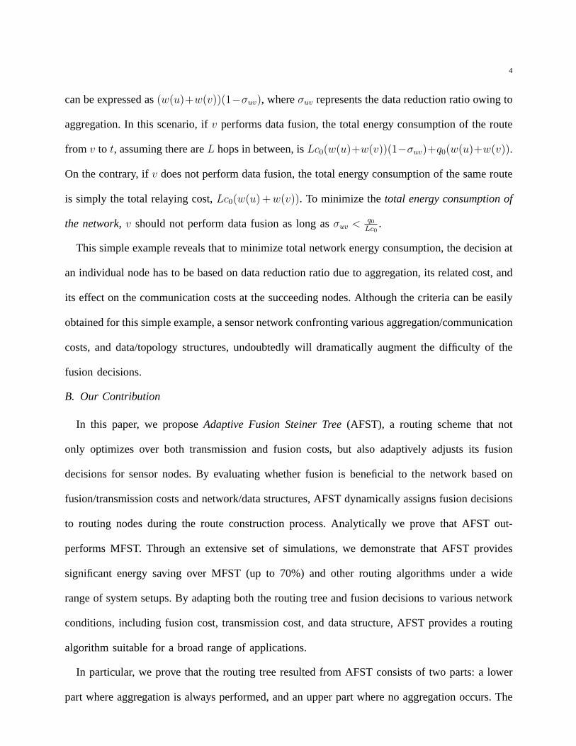
Fig. 4(a) summarizes the performance of all algorithms studied. The largerrc is, the more

strongly the network is connected. As we can see, MST wastes precious energy on data fusion at

numerous relaying nodes and hence incurs high cost when the data reduction is not high. On the

21

5 15 25 35 4570

75

80

85

90

95

100

105

110

Communication range rc (m)

Tot

al c

ost (

mJ)

MFSTAFSTSPTMSTSLT

(a) Total cost

5 15 25 35 45

1

1.05

1.1

1.15

1.2

1.25

1.3

1.35

1.4

Communication range rc(m)

Cos

t rat

io to

oth

er a

lgor

ithm

s

MFST vs. AFSTAFSTSLT vs. AFSTMST vs. AFSTSPT vs. AFST

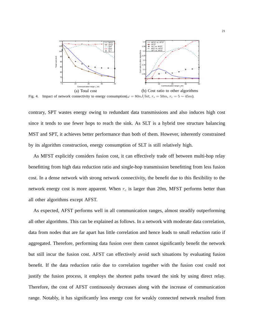
(b) Cost ratio to other algorithmsFig. 4. Impact of network connectivity to energy consumption(ω = 80nJ/bit, rs = 50m, rc = 5 ∼ 45m).

contrary, SPT wastes energy owing to redundant data transmissions and also induces high cost

since it tends to use fewer hops to reach the sink. As SLT is a hybrid tree structure balancing

MST and SPT, it achieves better performance than both of them. However, inherently constrained

by its algorithm construction, energy consumption of SLT is still relatively high.

As MFST explicitly considers fusion cost, it can effectively trade off between multi-hop relay

benefitting from high data reduction ratio and single-hop transmission benefitting from less fusion

cost. In a dense network with strong network connectivity, the benefit due to this flexibility to the

network energy cost is more apparent. Whenrc is larger than 20m, MFST performs better than

all other algorithms except AFST.

As expected, AFST performs well in all communication ranges, almost steadily outperforming

all other algorithms. This can be explained as follows. In a network with moderate data correlation,

data from nodes that are far apart has little correlation and hence leads to small reduction ratio if

aggregated. Therefore, performing data fusion over them cannot significantly benefit the network

but still incur the fusion cost. AFST can effectively avoid such situations by evaluating fusion

benefit. If the data reduction ratio due to correlation together with the fusion cost could not

justify the fusion process, it employs the shortest paths toward the sink by using direct relay.

Therefore, the cost of AFST continuously decreases along with the increase of communication

range. Notably, it has significantly less energy cost for weakly connected network resulted from

22

short communication range as well. It can be reasoned in the same way.

Fig. 4(b) illustrates the cost ratio of other algorithms to AFST. As shown in the figure, the

proposed AFST can save over40% energy compared to MST, up to35% energy to SPT, and

about 10% to SLT when connectivity degree is high. Compared with MFST, AFST can save

around 10% of energy in weakly connected environment while maintaining the same or better

performance when network is strongly connected.

C. Impact of Correlation Coefficient

Naturally, performing aggregation is futile in a network with no data redundancy (ρ = 0). Even

in a network with 100% data redundancy (ρ = 1), data fusion at all possible nodes may not bring

benefit because of the high fusion cost. In this simulation, we fix the transmission range of the

sensor nodes and study the impact of correlation coefficient to the performance of AFST. We

increase the correlation range,rs, from 0.2 to 2000m which corresponds to varyingρ from 0 to

1.

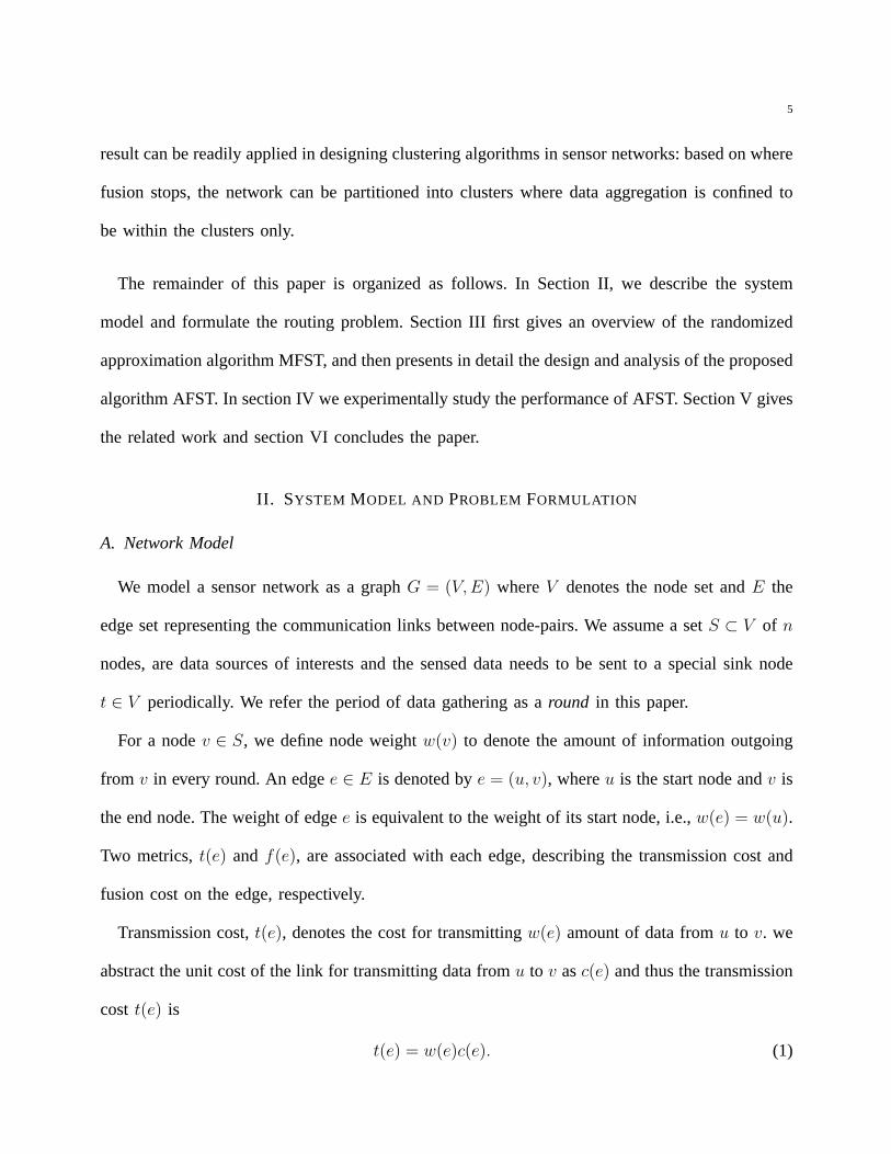
0.25 1 4 16 64 256 204850

100

150

200

Correlation range rs(m)

Tot

al c

ost (

mJ)

MFSTAFSTSPTSPT−nfSLT

(a) Low fusion cost (ω = 50nJ/bit)

0.25 1 4 16 64 256 204870

100

150

200

250

Correlation range rs(m)

Tot

al c

ost (

mJ)

MFSTAFSTSPTSPT−nfSLT

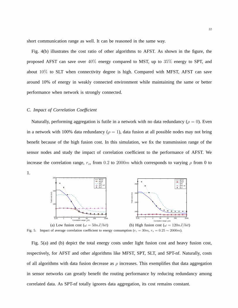
(b) High fusion cost (ω = 120nJ/bit)Fig. 5. Impact of average correlation coefficient to energy consumption (rc = 30m, rs = 0.25 ∼ 2000m).

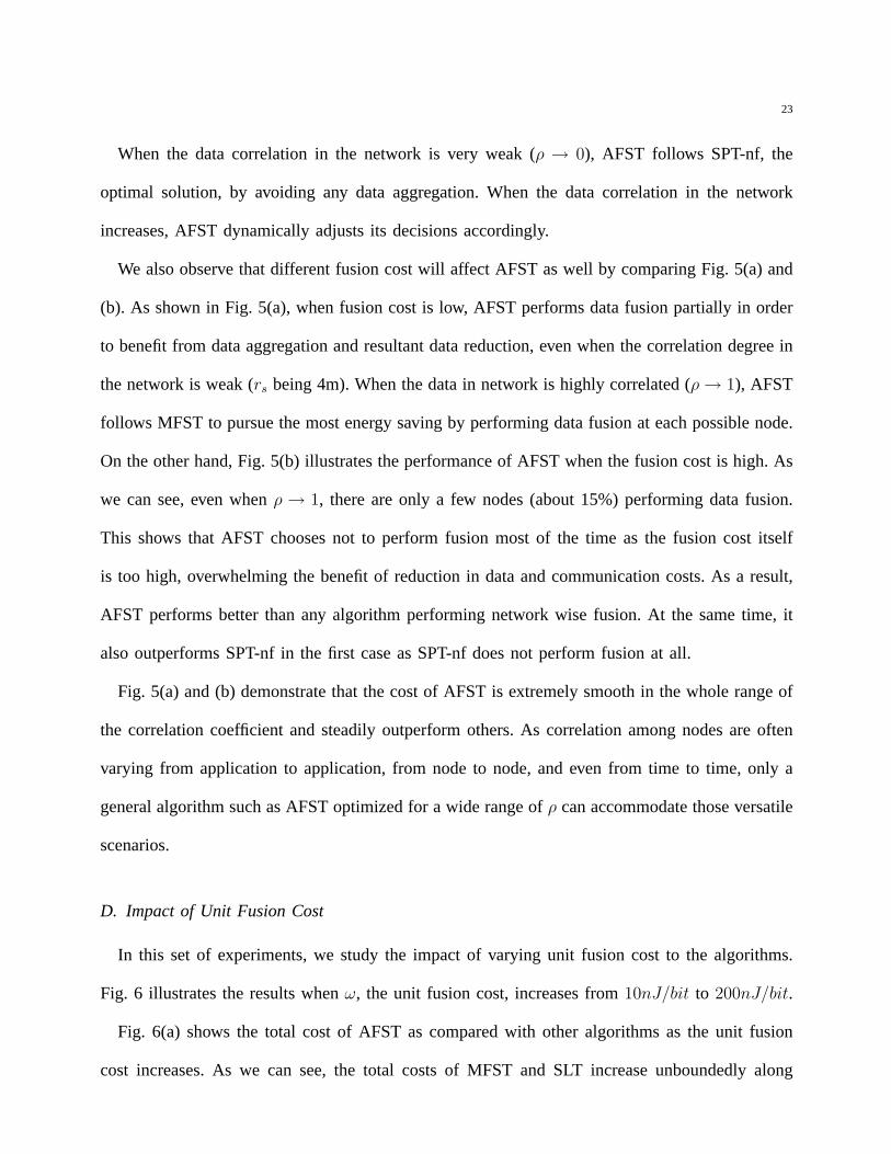
Fig. 5(a) and (b) depict the total energy costs under light fusion cost and heavy fusion cost,

respectively, for AFST and other algorithms like MFST, SPT, SLT, and SPT-nf. Naturally, costs

of all algorithms with data fusion decrease asρ increases. This exemplifies that data aggregation

in sensor networks can greatly benefit the routing performance by reducing redundancy among

correlated data. As SPT-nf totally ignores data aggregation, its cost remains constant.

23

When the data correlation in the network is very weak (ρ → 0), AFST follows SPT-nf, the

optimal solution, by avoiding any data aggregation. When the data correlation in the network

increases, AFST dynamically adjusts its decisions accordingly.

We also observe that different fusion cost will affect AFST as well by comparing Fig. 5(a) and

(b). As shown in Fig. 5(a), when fusion cost is low, AFST performs data fusion partially in order

to benefit from data aggregation and resultant data reduction, even when the correlation degree in

the network is weak (rs being 4m). When the data in network is highly correlated (ρ → 1), AFST

follows MFST to pursue the most energy saving by performing data fusion at each possible node.

On the other hand, Fig. 5(b) illustrates the performance of AFST when the fusion cost is high. As

we can see, even whenρ → 1, there are only a few nodes (about 15%) performing data fusion.

This shows that AFST chooses not to perform fusion most of the time as the fusion cost itself

is too high, overwhelming the benefit of reduction in data and communication costs. As a result,

AFST performs better than any algorithm performing network wise fusion. At the same time, it

also outperforms SPT-nf in the first case as SPT-nf does not perform fusion at all.

Fig. 5(a) and (b) demonstrate that the cost of AFST is extremely smooth in the whole range of

the correlation coefficient and steadily outperform others. As correlation among nodes are often

varying from application to application, from node to node, and even from time to time, only a

general algorithm such as AFST optimized for a wide range ofρ can accommodate those versatile

scenarios.

D. Impact of Unit Fusion Cost

In this set of experiments, we study the impact of varying unit fusion cost to the algorithms.

Fig. 6 illustrates the results whenω, the unit fusion cost, increases from10nJ/bit to 200nJ/bit.

Fig. 6(a) shows the total cost of AFST as compared with other algorithms as the unit fusion

cost increases. As we can see, the total costs of MFST and SLT increase unboundedly along

24

10 50 100 150 20040

60

80

100

120

140

160

Unit fusion cost ω (nJ/bit)

Tot

al c

ost (

mJ)

MFSTAFSTSPT−nfSLT

(a) Total cost

10 50 100 150 200

10

20

30

40

50

60

70

80

90

100

Unit fusion cost ω (nJ/bit)

Num

ber

of fu

sion

clu

ster

s

(b) Number of fusion clusters

10 50 100 150 2000

20

40

60

80

100

120

Unit fusion cost ω (nJ/bit)

Fus

ion

cost

(m

J)

MFSTAFSTSPT−nfSLT

(c) Fusion cost

10 50 100 150 20040

45

50

55

60

65

70

75

80

85

Unit fusion cost ω (nJ/bit)

Tra

nsm

issi

on c

ost (

mJ)

MFSTAFSTSPT−nfSLT

(d) Transmission costFig. 6. Impact of unit fusion cost to energy consumption(rc = 30m, rs = 20m, ω = 10 ∼ 200nJ/bit).

with the increase ofω, even though MFST has a lower slope. On the contrary, AFST follows the

performance curve of MFST first and then leans towards SPT-nf, the optimal solution when fusion

cost is high. The figure can be best explained when we jointly examine it with Fig. 6(b), which

depicts the number of clusters, the branches of the routing tree that always perform aggregation

on their nodes. All algorithms with network wise fusion are unable to stop fusion even when

fusion cost is extremely high. However, for AFST, as shown in Fig. 6(b), whenω is very small,

there are only two fusion clusters. This denotes that data fusion is performed almost on all nodes,

which takes advantage of the low fusion cost. Whenω increases, AFST increases the number of

fusion clusters and hence reduces the number of fusions due to reduced fusion benefit in order

to balance the fusion cost and transmission cost. And whenω is too large, AFST can achieve the

same constant cost as SPT-nf by completely stopping data fusion.

Fig. 6(c) and (d) provide us a closer look at the routing behaviors by breaking the total cost

into transmission and fusion costs. As both SLT and SPT-nf have fixed tree structure when the

network topology is determined, their transmission costs are fixed as well. Naturally, the fusion

cost of SLT increases linearly withω while there is no fusion cost in SPT-nf.

As MFST jointly explores the transmission and fusion costs to optimize the routes, it can

tradeoff between them. As a strategy, it can explore long one-hop transmission in order to reduce

the number of fusions and hence fusion cost. As a result, the transmission cost in MFST increases

in order to prevent the fast increase of fusion cost. Consequently, the increase of fusion cost

25

and total cost in MFST are significantly slower than SLT. However, whenω increases more and

fusion cost is dominant in the total cost, adjustment of routing tree structure will have insignificant

impact and hence MFST’s fusion cost increases almost linearly while its transmission cost remains

constant.

On the contrary, AFST can better balance the fusion and transmission costs by adjusting the

number of fusion clusters. When the unit fusion cost is insignificant, AFST effectively reduces its

transmission cost by fully exploiting data fusion. In this case, AFST’s cost is similar to that of

MFST. When the unit fusion cost continues to increase, AFST can reduce data fusion points and

employ more shortest paths for direct relaying. Therefore, while its transmission cost increases

rapidly, the fusion cost also decreases rapidly simultaneously. As a result, the total cost can be

kept low. When the unit fusion cost is extremely large, AFST simply approaches SPT-nf with no

node performing fusion and hence obtains zero fusion cost. In this case, the total cost equals to

the transmission cost and remains constant.

As described in Section II, fusion cost may vary widely from network to network, from

application to application. As an example, a temperature surveillance sensor network may have

little fusion cost to calculate the max, min, or average temperature. On the other hand, a wireless

video sensor network may incur significant fusion cost when performing image fusion. Our

experiments show that among all algorithms, AFST can adapt best to a wide range of fusion

costs and hence be applicable to a variety of applications.

E. Extreme Cases of Correlation Coefficient

In this set of experiments, we study the performance of AFST when the correlation coefficient

takes extreme values. We examine the scenario where there is no data redundancy (ρ → 0) and

the scenario of 100% data aggregation (ρ → 1). Fig. 7 summarizes the results. Two cases, with

or without fusion cost, are studied for each of the scenarios. In all cases,rc is varied from 5m to

26

45m, denoted by the x-axis. We users = 0.1m to simulate the case ofρ → 0 and rs = 2000m

to simulate the case ofρ → 1.

5 10 15 20 25 30 35 40 450

100

200

300

400

500

600

700

Conmmunication range rc(m)

Tot

al c

ost (

mJ)

MFSTAFST/SPTMSTSLT

(a) ρ → 0 without fusion cost

5 10 15 20 25 30 35 40 4530

35

40

45

50

55

60

65

Communication range rc(m)

Tot

al c

ost (

mJ)

MFST/AFSTSPTMSTSLT

(b) ρ → 1 without fusion cost

5 10 15 20 25 30 35 40 450

100

200

300

400

500

600

700

800

900

Communication range rc (m)

Tot

al c

ost (

mJ)

MFSTAFST/SPT−nfSPTSLT

(c) ρ → 0 with fusion cost

5 10 15 20 25 30 35 40 4570

72

74

76

78

80

82

84

86

Communication range rc(m)

Tot

al c

ost (

mJ)

MFSTAFSTSPTMSTSLT

(d) ρ → 1 with fusion costFig. 7. Total cost at extreme cases of data correlation (rc = 30m, ω = 80nJ/bit).

1) Without fusion cost:We first disregard fusion cost. The simulation results shown in Fig. 7(a)

and (b) concur with those described in [15]. In a weakly correlated network, SPT is the optimal

solution while MST is the worst. On the contrary, in a strongly correlated network, MST is the

optimal solution and SPT is the worst. Fig. 7(a) also shows that AFST is the same as the optimal

solution, SPT, in a weakly correlated network and has a gain factor of 3 compared with MFST.

Fig. 7(b) shows that both AFST and MFST closely approximate the optimal solution, MST. The

approximation ratio is within 5%, and they can save 10% energy compared with SLT.

2) With fusion cost:In this set of simulations, we include fusion cost and study the two extreme

scenarios again. We setω, the unit fusion cost, to be80nJ/bit.

Fig. 7(c) illustrates that AFST can achieve the optimal

0 20 40 60 80 100120140160

0.5

2

8

32

128

512

0

20

40

60

80

100

Correlation range rs (m)Unit fusion cost ω (nJ/bit)

Num

ber

of fu

sion

clu

ster

s

Fig. 8. The number of fusion clusters in AFST.

performance by avoiding data fusion completely compared

with all other algorithms with inefficient data fusion on

uncorrelated data.

When ρ → 1 as illustrated in Fig. 7(d), since the unit

fusion cost is comparable to the average of transmission

cost, AFST behaves similarly as MFST by performing

network wise data fusion, and performs better than all other algorithms.

27

F. The Number of Fusion Clusters in AFST

Fig. 8 illustrates the number of fusion clusters with varying correlation coefficient and unit

fusion cost. Whenρ → 0, the cluster number equals 100, denoting that no data fusion occurs.

When the unit fusion cost is small, the number of fusion clusters decreases rapidly with the

increase ofρ. Whenρ approaches 1, the cluster number becomes 1, meaning that all nodes will

perform fusion and the network becomes a full fusion tree. At the same time, when unit fusion cost

increases, AFST will tradeoff the fusion cost with transmission cost. As a result, the decreasing

of the cluster number slows down. For example, forω = 80nJ/bit, a unit fusion cost comparable

to the average unit transmission cost, there are 33 fusion clusters whenρ → 1. This means on

average, there are only three nodes in a cluster performing data fusion. The fused data are then

forwarded to the sink via shortest paths directly with simple relaying. Ifω keeps increasing, fewer

nodes perform fusion to avoid the high fusion cost.

V. RELATED WORK

If the complete knowledge of all data correlations is available in advance at each source,

theoretically the best routing strategy is to use a distributed source coding typified by Slepian-

Wolf coding [24]. In this technique, compression is done at the original sources in a distributed

manner to achieve the minimum entropy and hence avoid the need for data aggregation on the

intermediate nodes. An optimal rate allocation algorithm for nodes in the network is proposed in

[15] and SPT is employed as the routing scheme. However, implementation of distributed source

coding in a practical setting is still an open problem and likely to incur significant additional cost

because of the requirement on the knowledge of network wise correlation.

Routing with data aggregation can be generally classified into two categories: routing-driven and

aggregation-driven. Routing-driven algorithms [7–9, 12, 13] emphasize source compression at each

individual node and aggregation occurs opportunistically when routes intersect. On the contrary,

28

routing paths in aggregation-driven algorithms [14–16] are heavily dependent on data correlation

in order to fully benefit from information reduction resulting from data aggregation. In [15], the

authors proved that the minimum-energy data gathering problem is NP-complete by applying

reduction set-cover problem and claimed that the optimal result is between SPT and the travelling

salesman path. In [14], a hierarchical matching algorithm is proposed resulting in an aggregation

tree with a logarithmic approximation ratio to the optimal for all concave aggregation functions.

In this model, each node can theoretically obtain the joint entropy of its subtree to receive the

maximal aggregation ratio. However, aggregation only depends on the number of nodes in the

subtree rooted at the aggregation node regardless of the correlation among the data.

Indeed, the idea of embedding fusion decisions in routing has been implicitly explored in the

literature. For example, LEACH [7] is a cluster-based protocol, in which sensors directly send

data to cluster heads where data fusion is performed. Aggregated data is then delivered to the

sink through multi-hop paths. The authors of [16] proposed an optimal algorithm MEGA for

foreign-coding and an approximating algorithm LEGA for self-coding. In MEGA, each node

sends raw data to its encoding point using directed MST, and encoded data is then transmitted

to the sink through SPT. LEGA uses SLT [25, 26] as the data gathering topology, and achieves

2(1 +√

2) approximation ratio for self-coding. LEGA and MEGA implicitly assume that fusion

stops after first aggregation as encoded data cannot be recoded again. However, the decision

regarding fusions in these schemes are rather static and cannot adapt to network/data structure

changes. As demonstrated earlier, this decision shall be based on various conditions of the networks

in order to minimize energy consumption.

VI. CONCLUSION

In this paper, we propose AFST, a routing algorithm for gathering correlated data in sensor

networks. AFST not only optimizes over both the transmission and fusion costs, but also adaptively

29

adjusts fusion decisions for sensor nodes as to whether fusion shall be performed. Generalized

from MFST, an algorithm guarantees an approximation ratio of54log(n+1) to the optimal solution,

AFST is analytically shown to be a better algorithm than its ancestor. Extensive experiments show

that AFST achieves near optimal solutions under various networking conditions, including broad

scopes of fusion/transmisison costs and network/data structures.

Furthermore, our analytical result indicates that AFST partitions the routing tree into two distinct

parts based on whether aggregation is performed or not. Naturally, AFST also provides a clustering

scheme with near optimal routing performance, where fusion can be confined within the clusters

only.

As an ongoing effort, we are quantifying theoretically the performance improvement of AFST

over MFST. In our future work, we plan to develop an online algorithm based on AFST that can

be executed in a distributed manner by sensor nodes.

REFERENCES

[1] H. Luo, J. Luo, Y. Liu, and S. K. Das, “Routing correlated data with adaptive fusion in wireless sensor networks,” in

Proceedings of the 3rd ACM/SIGMOBILE International Workshop on Foundation of Mobile Computing, Cologne, Germany,

Aug. 2005.

[2] H. Luo, Y. Liu, and S. K. Das, “Routing correlated data with fusion cost in wireless sensor networks,”IEEE Transactions

on Mobile Computing, to appear.

[3] C. Chong and S. Kumar, “Sensor networks: Evolution, opportunities, and challenges,”Proceedings of the IEEE, vol. 91,

no. 8, Aug. 2003.

[4] I. Akyildiz, W. Su, Y. Sankarasubramaniam, and E. Cayirci, “A survey on sensor networks,”IEEE Communications Magazine,

vol. 40, no. 8, Aug. 2002.

[5] W. Heinzelman, J. Kulik, and H. Balakrishnan, “Adaptive protocol for information dissemination in wireless sensor networks,”

in Proceedings of ACM Mobicom, Seattle, WA, Aug. 1999.

[6] A.A. Ahmed, H. Shi, and Y. Shang, “A survey on network protocols for wireless sensor networks,” inProceedings of the

IEEE ITRE’03, Newark, NJ, Aug. 2003.

[7] W.R. Heinzelman, A. Chandrakasan, and H. Balakrishnan, “Energy-efficient communication protocol for wireless microsensor

networks,” inProceedings of the 33rd Annual Hawaii International Conference on System Sciences, Maui, HI, Jan. 2000.

[8] B. Krishnamachari, D. Estrin, and S. Wicker, “Impact of data aggregation in wireless sensor networks,” inProceedings of

the 22nd International Conference on Distributed Computing Systems, Vienna, Austria, July 2002.

[9] A. Scaglione and S. D. Servetto, “On the interdependence of routing and data compression in multi-hop sensor networks,”

in Proceedings of ACM MobiCom, Altanta, GA, Sept. 2002.

[10] S. Pattem, B. Krishnamachari, and R. Govindan, “The impact of spatial correlation on routing with compression in wireless

sensor networks,” inProceedings of IPSN’04, Berkeley, CA, Apr. 2004.

[11] W. Zhang and G. Cao, “Dctc: Dynamic convoy tree-based collaboration for target tracking in sensor networks,”IEEE

Transactions on Wireless Communication, vol. 3, no. 5, pp. 1685–1701, Sept. 2004.

30

[12] C. Intanagonwiwat, D. Estrin, R. Govindan, and J. Heidemann, “Impact of network density on data aggregation in wireless

sensor networks,” inProceedings of ICDCS’02, Vienna, Austria, July 2002.

[13] C. Intanagonwiwat, R. Govindan, D. Estrin, J. Heidemann, and F. Silva, “Directed diffusion for wireless sensor networking,”

IEEE/ACM Transactions on Networking, vol. 11, no. 1, Feb. 2003.

[14] A. Goel and D. Estrin, “Simultaneous optimization for concave costs: Single sink aggregation or single source buy-at-bulk,”

in Proceedings of ACM-SIAM Symposium on Discrete Algorithms, Baltimore, MD, Jan. 2003.

[15] R. Cristescu, B. Beferull-Lozano, and M. Vetterli, “On network correlated data gathering,” inProceedings of IEEE Infocom,

Hongkong, China, Mar. 2004.

[16] P.V. Rickenbach and R. Wattenhofer, “Gathering correlated data in sensor networks,” inProceedings of ACM DIALM-

POMC’04, Philadelphia, PA, Oct. 2004.

[17] Y. Yu, B. Krishnamachari, and V. Prasanna, “Energy-latency tradeoff for data gathering in wireless sensor networks,” in

Proceedings of IEEE Infocom, Hongkong, China, Mar. 2004.

[18] S. Lindsey and C. S. Raghavendra, “Pegasis: Power-efficient gathering in sensor information systems,” inProceedings of

IEEE Aerospace Conference, Big Sky, MT, Mar. 2002.

[19] W. Zhang and G. Cao, “Optimizing tree reconfiguration for mobile target tracking in sensor networks,” inProceedings of

IEEE Infocom, Hongkong, China, Mar. 2004.

[20] A. Wang, W. B. Heinzelman, A. Sinha, and A. P. Chandrakasan, “Energy-scalable protocols for battery-operated microsensor

networks,” Journal of VLSI Signal Processing, vol. 29, no. 3, Nov. 2001.

[21] D. W. Carman, P. S. Kruus, and B. J. Matt, “Constraints and approaches for distributed sensor network security,”NAI Labs

Technical Report 00-010, Sept. 2000.

[22] A. Meyerson, K. Munagala, and S. Plotkin, “Cost-distance: Two metric network design,” inProceedings of the 41st Annual

Symposium on Foundations of Computer Science, Redondo Beach, CA, Nov. 2000.

[23] C. Papadimitriou and K. Steiglitz,Combinatorial Optimization: Algorithms and Complexity, Dover Publications Inc, 1998.

[24] S. S. Pradhan and K. Ramchandran, “Distributed source coding using syndromes (DISCUS): Design and construction,”

IEEE Transactions on Information Theory, vol. 49, no. 3, Mar. 2003.

[25] A. Goel and K. Munagala, “Balancing steiner trees and shortest path trees online,” inProceedings of the 11th ACM-SIAM

symposium on Discrete Algorithms, San Francisco, CA, Jan. 2000.

[26] B. Raghavachari S. Khuller and N. Young, “Balancing minimum spanning and shortest path trees,” inProceedings of the

4th ACM-SIAM symposium on Discrete Algorithms, Austin, TX, Jan. 1993.

[27] “http://www.eecs.umich.edu/ panalyzer/,” .

[28] T. Austin, E. Larson, and D. Ernst, “Simplescalar: an infrastructure for computer system modeling,”Computer, vol. 35, no.

2, pp. 59, Feb. 2002.

[29] L.J. Chipman, T.M. Orr, and L.N. Graham, “Wavelets and image fusion,” inProceedings of the International Conference

on Image Processing, Washington DC, USA, Oct. 1995.

[30] W. B. Pennebaker and J. L. Mitchell,JPEG: Still Image Data Compression Standard, Van Nostrand Reinhold, 1993.

[31] J. M. Shapiro, “Embedded image coding using zerotrees of wavelet coefficients,”IEEE Transactions on Signal Processing,

vol. 41, no. 12, Dec. 1993.

APPENDIX

We have performed a series of experiments to investigate the aggregation cost in sensor net-

works. Our platform used is Sim-panalyzer [27], an extension of Simple Scalar [28] for power

analysis. Simple Scalar is a well established architectural simulator that provides cycle-level tool

sets for detailed processor-architecture study. As its extension, Sim-panalyzer provides analytical

31

power simulation models for ARM CPU and Alpha CPU. In our experiments, we choose Stron-

gARM SA-1110 as our embedded core as it is commonly used for high performance sensor node

design in academic research and industrial development.

A. Measurement Model for Data Aggregation

We first detail the model of data aggregation processInput Data Raw Data

Decompression Data Filtering

Compression

Fusion Algorithm

Transmission

Fig. 9. Measurement model for data aggregation.

used in our simulation. As illustrated in Fig. 9, we assume

that each sensor is capable of data sensing, pre-processing,

and data aggregation. A sensor node will compress its local

raw data before transmitting it on the route back to the sink.

If it receives data from another node, in a compressed form,

to perform data aggregation, the node shall decompress the

data first and perform the designated aggregation algorithm with its own raw data. The aggregated

data will then be compressed and routed to the next hop. In this model, the aggregation cost is

composed of two parts, marked in gray in Fig. 9, the cost for decompressing the input data and

the cost for performing the fusion algorithm itself. In the following, we will only focus on these

two parts.

Energy consumption of a system contains static power dissipation and dynamic power dissipa-

tion. Dynamic power dissipation denotes the application processing energy with given instruction

set and data set. Evidently, this part is the investigating target of our experiment. Equation (11)

is a model for dynamic power dissipation commonly employed in energy measurement [20].

Etotal = CtotalV2dd + Vdd(I0e

VddnVT )(

N

f). (11)

Here,N represents the number of cycles for executing the algorithm with the given data set. It is

determined by the algorithm complexity and affected by the compiling method.Ctotal denotes the

total switched capacitance during the execution of the algorithm.Ctotal is proportional toN and

32

it is also affected by the switching activity parameter.Vdd andf are the core supply voltage and

clock frequency of the CPU, respectively.VT denotes thermal voltage.I0 andn are core specific

which we assign1.196mA and 21.26 according to [20]. The SA-1110 core can be configured

to various combinations of supply voltage and system clock. In our experiment we use 100MHz

clock and 1.5V for core voltage. We have performed simulations using other configurations and

the simulation results are similar.

B. Image Fusion

One of our experiments is wavelet-based image fusion. Wavelet-based image fusion is generally

considered as the most efficient algorithm for image fusion and different approaches have been

proposed [29]. In our experiment, we simulate a simple and efficient method described in [29].

According to the measurement model illustrated in Fig. 9, a fusion node will use Discrete Wavelet

Transformation (DWT) to generate wavelet coefficients from local image. To perform fusion with

another node’s data, the node will use Zerotrees expansion to decompress the input data into

wavelet coefficients. Given the wavelet coefficients of the two input images, the averages of

these coefficients are computed as those for the fusion result. While this algorithm is simple,

it provides a lower bound on the computation cost. More complex algorithms for better fusion

result will undoubtedly incur even higher cost. Consequently, the aggregation cost is the cost of

the decompression process and the merging process.3

(a) Input image (b) Local image (c) Fused imageFig. 10. Image Fusion Example.

3The cost of the final Zerotree compression on the merged data shall not be considered as part of the fusion cost as the nodewould perform Zerotree compression on its local data even if fusion was not performed.

33

The gray scale images depicted in Fig. 10 are used in the simulation. Fig. 10(a) is the input

image representing data from another node. Notice that it has a blurred area at the top-left corner.

Fig. 10(b) is the local image at the fusion node, with a blurred area at the bottom-left corner. Fig.

10(c) is the fused image by performing the aforementioned fusion algorithm on Fig. 10(a) and

(b). Notice that in the fused image, the blurred areas are effectively eliminated.

2000 4000 6000 8000 10000 120000

1

2

3

4

5

6

7

8x 10

−3

Input data size (byte)

Ene

rgy

cost

(J)

(a) Energy cost

2000 4000 6000 8000 10000 1200020

30

40

50

60

70

80

90

100

110

120

Input data size (byte)

Ene

rgy

cost

on

per

bit (

nJ)

(b) Per bit energy costFig. 11. Wavelet image fusion cost.

Fig. 11(a) and (b) depict our experiment results. During our simulation, we scaled the image

content from64× 64 pixels to220× 220 pixels. Reflected on the X axis of the figures, it is the

total data size in byte of the two input images of the fusion algorithm. As we perform two level

DWT and apply the embedded coding scheme [30, 31] using Zerotrees, the compression ratio is

approximately 8:1. Therefore, the X axis ranges from 1 KB (corresponding to64× 64 pixels) to

12 KB (corresponding to220×220 pixels) as the summation of two image sizes. The total image

fusion energy consumption inJoule is shown in Fig. 11(a) while the per bit energy cost is shown

in Fig. 11(b). As we can see, the total image fusion cost monotonically increases with the input

data size. Fig. 11(b) shows that the per bit energy cost remains roughly constant at75nJ/bit,

comparable to per bit communication cost reported in the literature [7, 20]. The irregular variations

of per bit energy cost between consecutive measurements (image sizes) are due to the Zerotrees

encoding scheme.

We have also performed study on other fusion algorithms such as byte-wise Huffman coding.

34

The result is also on the order of tens ofnJ/bit. We omit the details here due to space limit.

From our experimental study, we can conclude that the fusion cost for certain sensor networks is

comparable to the transmission cost. Therefore, the impact of fusion cost to energy efficient data

gathering in sensor networks is an important area needed to be carefully investigated.