1 American Options

Most traded stock options and futures options are of American-type while most index optionsare of European-type.The central issue is when to exercise?From the holder point of view, the goal is to maximize holder’s profit (Note that here

the writer has no choice!)

1.1 Some General Relations (for the no dividend case)

The Call Option:

1. CA (0) ≥ (S (0)−K)+

Proof:

(1) CA (0) ≥ 0 (optionality);

(2) If CA (0) < S (0)−K (assuming S (0) > K)

buy the option at CA (0)

then, exercise immediately. This leads to

profit: S (0)−K

and

the net profit: S (0)−K − CA (0) > 0

which gives rise to an arbitrage opportunity.

Hence, the no-arbitrage argument yields

CA (0) ≥ (S (0)−K)

2. S (0) ≥ CA (0)

Proof:

If S (0) < CA (0) , buy S (0) and sell CA (0)

yielding a net profit > 0 at t = 0.

Because the possession of the stock

can always allow the deliverance of the stock

to cover the exercise if exercised,

then we are guaranteed to have a positive future profit.

Hence, an arbitrage opportunity.

1

3. CA (0) ≥ CE (0) with the same maturity T and strike K.

cf. CE (0) ≥ (S (0)−KB (0, T ))+ , ∴ CA (0) ≥ (S (0)−KB (0, T ))+

4. If the stock has no dividend payment, and the risk-free interest rate is positive, i.e.,B (0, T ) < 1 ∀T > 0, then one should never prematurely exercise the American call,i.e.,

CA (0) = CE (0)

Proof:

(1) CA (0) ≥ CE (0) ≥ (S (0)−KB (0, T ))+ – i.e., the call is "alive"

(2) If exercised now =⇒ the profit S (0)−K – i.e., the call is "dead"

Note that

S (0)−KB (0, T )| {z }alive

> S (0)−K| {z }dead

therefore, it is worth more "alive" than "dead"

Note that

(a) Question: Should one exercise the call if S (0) > K and if he believes the stockwill go down below K?

No! If exercise,(profit)1 = S (0)−K

If sell the option,(profit)2 = CA (0)

SinceCA (0) ≥ (S (0)−K)+

one should sell the option rather than exercise it!

(b) With dividend, early exercise may be optimal

2

(c) Intuition – consider paying K to get a stock now vs. paying K to get a stocklater, one gets the interest on K , therefore, the difference is

KerT −K if wait

5. For two American call options, CA (t,K, T1) and CA (t,K, T2) ,with the same strike Kon the same stock but with different maturities T1 and T2, then we have

CA (0,K, T1) ≥ CA (0,K, T2)

if T1 ≥ T2.

The Put Option:

1. PA (0) ≥ (K − S (0))+

cf. PE (0) ≥ (KB (0, T )− S (0))+

Proof:

If PA (0) < K − S (0) ,

buy PA and exercise immediately, yielding, then, the total cash flow:

−PA (0)| {z }buy put

+ (K − S (0))| {z }exercise

> 0

giving rise to an arbitrage opportunity.

2. PA (0) ≤ K

3. PA (0) ≥ PE (0)

Note that: For a put, the profit is bounded by K. This fact limits the benefit fromwaiting to exercise and its financial consequence is that one may exercise early if S (0)is very small.

3

4. Put-call parity for American options:

S (0)−K ≤ CA − PA ≤ S0 −Ke−rT

Put-call parity for American options on an non-dividend-paying stock:

(a) PA (0) + S (0)−KB (0, T ) ≥ CA (0) ;

(b) CA (0) ≥ PA (0) + S (0)−K

i.e.,S (0)−K ≤ CA (0)− PA (0) ≤ S0 −KB (0, T )

Proof:(1) PA (0) ≥ PE (0) = CE (0)− S (0) +KB (0, T )

∵ CE (0) = CA (0)

=⇒ PA (0) ≥ CA (0)− S (0) +KB (0, T )

4

(2) Consider portfolio:

long one call

short one put

short the stock

hold K dollars in cash

i.e.,CA (0)| {z }Neverexercisedearly

− PA (0)| {z }Can beexercisedearly

− S (0) +K

If the put is exercised early at t∗, our position is

CA (t∗)− [K − S (t∗)]− S (t∗) +KB (0, t∗)−1 = CA (t

∗) +K(B (0, t∗)−1 − 1) ≥ 0

=⇒ liquidated with net positive profit (note that the above inequalityholds “>” strictly if S (t∗) > 0 and t∗ = 0)

If not exercised earlier, at maturity t = T, we have

(i) If S (T ) ≤ K,

profit = 0− [K − S (T )]− S (T ) +KB (0, T )−1 = K¡B (0, T )−1 − 1¢ > 0

(ii) If S (T ) > K,

profit = (S (T )−K)− 0− S (T ) +KB (0, T )−1 = K¡B (0, T )−1 − 1¢ > 0

therefore, the payoff of the portfolio is positive or zero,

=⇒ the present value of the portfolio ≥ 0, i.e.,CA (0)− PA (0)− S (0) +K ≥ 0

Combining (1) and (2) =⇒S (0)−K ≤ CA (0)− PA (0) ≤ S0 −KB (0, T )

QED

Note that: If the stock is dividend-paying, for European options, we have

CE (0)− PE (0) = P.V. [S (T )]−KB (0, T )

5

where P.V. [S (T )] is the present value of the stock whose price at T is S (T ) , e.g., If thereis a dividend D (t1) at t1, then

P.V. [S (T )] = S (0)−D (t1)B (0, t1)

for American options, we have

CA (0)− PA (0) ≤ S0 −KB (0, T )

which is unchanged by dividend, however, in general

P.V. [S (T )]−K ≤ CA (0)− PA (0) ≤ S0 −KB (0, T )

1.2 American Calls

1.2.1 Time Value

Consider American calls on no-dividend-paying stocks:

Consider the following strategy: Exercise it at maturity no matter what (obviously,suboptimal if K > S (T )), the present value of the American call under this strategy is:

P.V. [S (T )−K] = S (0)−KB (0, T )

which is equivalent to a forward.

The time value of an American call on a stock without dividends is

T.V. (0) = CA (0)− [S (0)−KB (0, T )]

Note thatT.V. (0) ≥ 0

this is becauseCA (0) ≥ CE (0) ≥ (S (0)−KB (0, T ))+

∴ T.V. (0) ≥ 0

6

If S (0)¿ K, then T.V. is highIf S (0)À K, then there is a high probability of expiring in-the-money, therefore,

CA (0) & S (0)−KB (0, T )

i.e., T.V. ≈ 0.

1.2.2 Dividends

Result: Given interest rate r > 0, it is never optimal to exercise an American call betweenex-dividends dates or prior to maturity.

Proof:Strategy 1: Exercise immediately,

(the value)1 = S (0)−K

Strategy 2: Wait till just before the ex-dividend date, and exercise for sure (evenif out-of-money)

(the value)2 = Sc (t)−K

where Sc (t) is the cum stock price just before going ex-dividend. Therefore, the presentvalue is

S (0)−KB (0, t)

Since B (0, t) < 1,

the value of Strategy 2 > the value of Strategy 1

therefore, it is best to wait.Next question: to exercise at anytime after the exdividend date and prior to maturity?

The same argument leads to the same conclusion: best to wait.

7

Question: To exercise or not to exercise?

If exercised just prior to the ex-dividend date,

the value = S (t)−K

= Se (t) +Dt −K

If not exercised,

the value = C (t) (based on the ex-div stock price)

C (t) = Se (t)−KB (t, T ) + T.V. (t)| {z }Time value at time t

Since it should be exercised if and only if the exercised value > the value not exercised, i.e.,

Se (t) +Dt −K > Se (t)−KB (t, T ) + T.V. (t)

=⇒Dt > K (1−B (t, T )) + T.V. (t) > 0 (1)

therefore, exercise is optimal at date t iff the dividend is greater than the interest lost on thestrike price K (1−B (t, T )) plus the time-value of the call evaluated using the ex-dividendstock price.

Note that

1. If Dt = 0 (i.e., no dividend) , Eq. (1) does not hold. Hence, never exercise early.

2. Exercise is optimal iff the dividend is large enough (> interest loss + T.V.), therefore,if the dividend is small, time-to-maturity is large, it is unlikely to exercise early.

1.3 American Puts

1.3.1 Time Value (if no dividend)

T.V. (0) = PA (0)− [KB (0, T )− S (0)]| {z }the present valueof exercising

the American putfor sure at maturity

≥ 0

PA (0) ≥ PE (0) ≥ (KB (0, T )− S (0))+

8

If S (0)À K, then T.V . is large, best to waitIf S (0)¿ K, then T.V. is small

1.3.2 Dividend:

Suppose Dt is the dividend per share at time t. The present value of exercising the Americanput for sure at maturity is

P.V. [K − S (T )] = KB (0, T )− [S (0)−DtB (0, t)]

Note that the dividend leads to a stock price drop, hence, added value for the put. Thetime-value of the put is

T.V. (0) = PA (0)− {KB (0, T )− [S (0)−DtB (0, t)]}

To exercise or not to exercise?

1. if exercise: the value is K − S (0)

2. if not exercise,

PA (0) = KB (0, T )− [S (0)−DtB (0, t)] + T.V. (0)

It is optimal to exercise if and only if

K − S (0) > PA (0)

i.e.,K − S (0) > KB (0, T )− [S (0)−DtB (0, t)] + T.V. (0)

orK (1−B (0, T ))| {z }Interest earned

due to early exercise

> DtB (0, t)| {z }Dividend lostdue to exercise

+ T.V. (0) (2)

Results:

9

1. It may be optimal to exercise prematurely even if the stock pays no dividends.

Proof: If Dt = 0, Eq. (2) becomes

K (1−B (0, T )) > T.V. (0)

if T.V. (0) is small, then, early exercise.

2. Dividends tend to delay early exercise.

Proof: As Dt increases,

K (1−B (0, T )) > DtB (0, t) + T.V. (0)

may not hold. Hence, to wait.

3. It never pays to exercise just prior to an ex-dividend date.

Proof: Consider the following two strategies:

(a) Strategy 1: Exercise just before the ex-dividend date,

(value)1 = K − [Se (t) +Dt]

Strategy 2: Exercise just after the ex-dividend date,

(value)2 = K − Se (t)

Since(value)2 > (value)1

one should exercise after the ex-dividend date.

1.4 Valuation Using a Binomial Tree

Consider an American option with payoff f (ST ) :

10

u = e

³r−σ2

2

´δt+σ

√δt

d = e

³r−σ2

2

´δt−σ√δt

At the S0u-node,

The option is worth½exercise: f (S0u) , “dead”not exercise: e−rδt (qf (S0u2) + (1− q) f (S0ud)) , “alive”

Compare these two values, choose the larger one, i.e., the value is

V+ = max©f (S0u) , e

−rδt ¡qf ¡S0u2¢+ (1− q) f (S0ud)¢ª

Similarly, at the S0d-node,

V− = max

f (S0d)| {z }exercised at t=δt

, e−rδt¡qf (S0ud) + (1− q) f

¡S0d

2¢¢| {z }

not exercise at t=δt

At t = 0,

V0 = max

f (S0)| {z }exercised at t=0

, e−rδt (qV+ + (1− q)V−)| {z }not exercise at t=0

Note that, for an American call,

1. If no dividend,CA (0) = CE (0)

2. If there are dividends,

11

3. Computational complexity:

N.B. The adaptive mesh methods: a high resolution (small ∆t) tree is graftedonto a low resolution (large ∆t) tree. This yields numerical efficiency over regularbinomial or trinomial trees. In particular, for American options, there is a need forhigh resolution close to strike price and to maturity.

1.5 Valuation Using PDE

Consider an American option with an arbitrary payoff f (ST ) . V (S, t) denotes its value attime t.Portfolio:

One American option

∆ shares of the stock

therefore,Π = V −∆S

dΠ− rΠdt| {z }profit in excess of the risk-free rate

=

µVt +

1

2σ2S2VSS − r (V −∆S)

¶dt+ (VS −∆) dS

Choose

∆ =∂V

∂S

then

dΠ− rΠdt =

µVt +

1

2σ2S2VSS − r (V − VSS)

¶dt

=

µVt +

1

2σ2S2VSS + rSVS − rV

¶dt

≡ LBSV dt

12

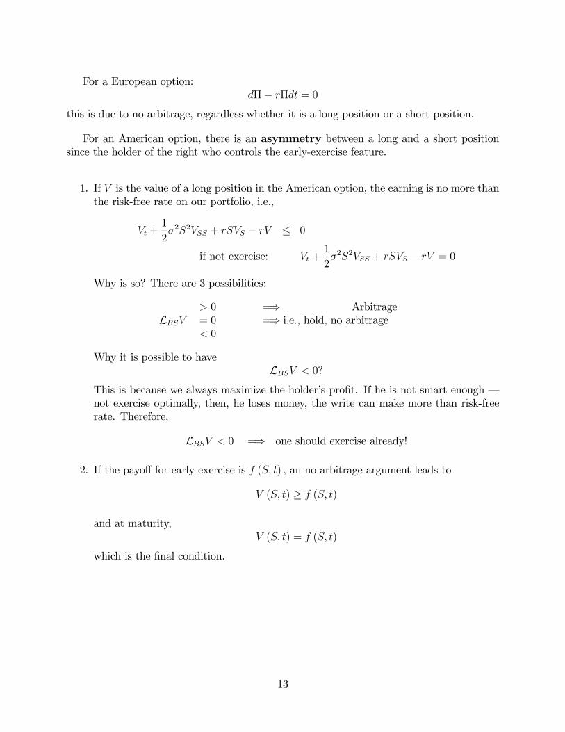
For a European option:dΠ− rΠdt = 0

this is due to no arbitrage, regardless whether it is a long position or a short position.

For an American option, there is an asymmetry between a long and a short positionsince the holder of the right who controls the early-exercise feature.

1. If V is the value of a long position in the American option, the earning is no more thanthe risk-free rate on our portfolio, i.e.,

Vt +1

2σ2S2VSS + rSVS − rV ≤ 0

if not exercise: Vt +1

2σ2S2VSS + rSVS − rV = 0

Why is so? There are 3 possibilities:

LBSV> 0 =⇒ Arbitrage= 0 =⇒ i.e., hold, no arbitrage< 0

Why it is possible to haveLBSV < 0?

This is because we always maximize the holder’s profit. If he is not smart enough –not exercise optimally, then, he loses money, the write can make more than risk-freerate. Therefore,

LBSV < 0 =⇒ one should exercise already!

2. If the payoff for early exercise is f (S, t) , an no-arbitrage argument leads to

V (S, t) ≥ f (S, t)

and at maturity,V (S, t) = f (S, t)

which is the final condition.

13

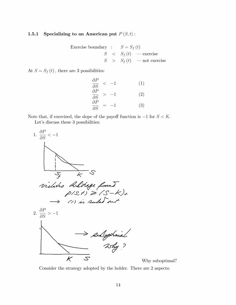
1.5.1 Specializing to an American put P (S, t) :

Exercise boundary : S = Sf (t)

S < Sf (t) – exercise

S > Sf (t) – not exercise

At S = Sf (t) , there are 3 possibilities:

∂P

∂S< −1 (1)

∂P

∂S> −1 (2)

∂P

∂S= −1 (3)

Note that, if exercised, the slope of the payoff function is −1 for S < K.Let’s discuss these 3 possibilities:

1.∂P

∂S< −1

2.∂P

∂S> −1

Why suboptimal?

Consider the strategy adopted by the holder. There are 2 aspects:

14

(a) day-to-day arbitrage-based hedging, which leads to the BS equation, i.e., "="holds,

LBSV = 0

(b) Exercise strategy: The boundary condition is

P (Sf (t) , t) = K − Sf (f)

the value of the option near S = Sf (f) can be increased by choosing a smallervalue for Sf , therefore

As P increases,∂P

∂Sdecreases

=⇒ ∂P

∂S= −1 at S = Sf (t)

which can be better justified using stochastic control theory, optimal stoppingproblems or game theory.Note that the payoff is a solution:i.e., LBSP ≤ 0 when P = K − S for S < K. This can be seen by substitutingP = K − S into

Pt +1

2σ2S2PSS + rsPS − rP

= rS × (−1)− r (K − S)

= −rK < 0

∴ LBSP ≤ 0 for P = K − S

Now the solution is specified as follows. Dividing S into 2 distinct regions:

15

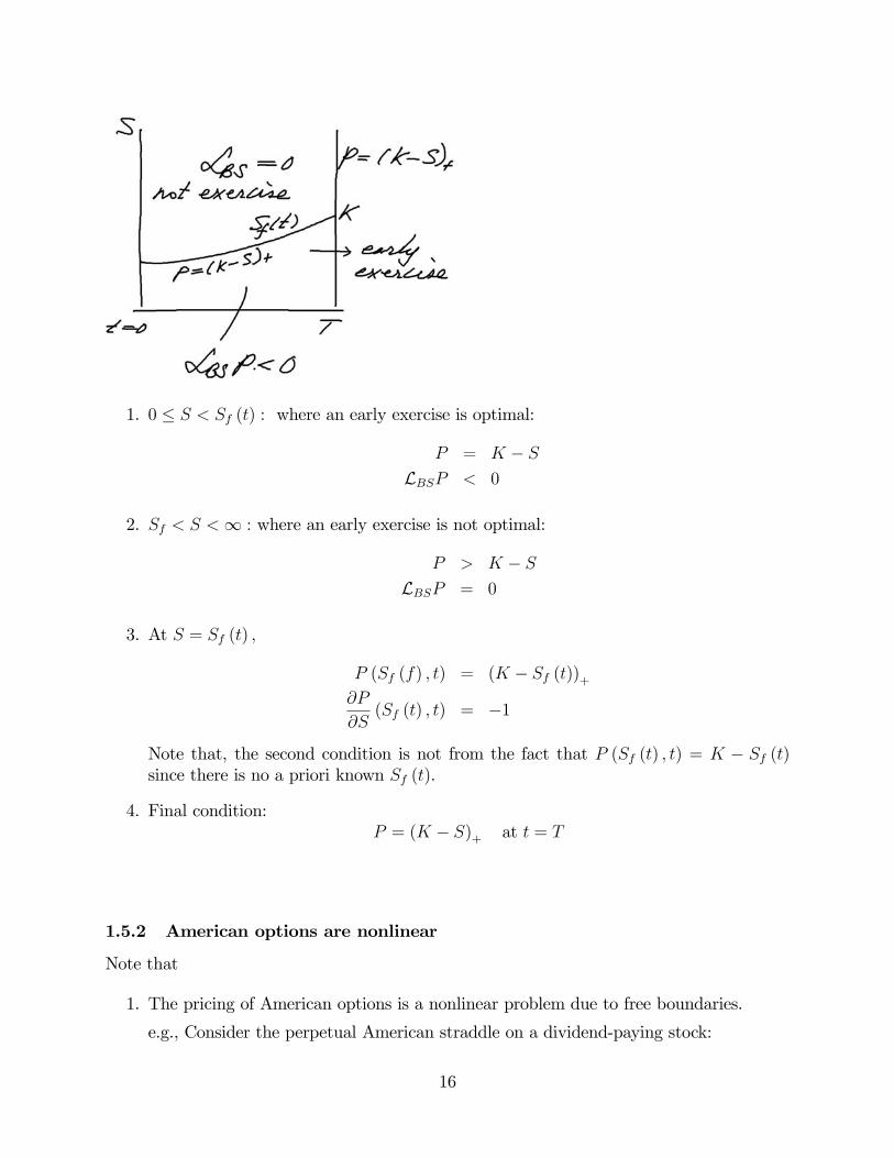
1. 0 ≤ S < Sf (t) : where an early exercise is optimal:

P = K − S

LBSP < 0

2. Sf < S <∞ : where an early exercise is not optimal:

P > K − S

LBSP = 0

3. At S = Sf (t) ,

P (Sf (f) , t) = (K − Sf (t))+∂P

∂S(Sf (t) , t) = −1

Note that, the second condition is not from the fact that P (Sf (t) , t) = K − Sf (t)since there is no a priori known Sf (t).

4. Final condition:P = (K − S)+ at t = T

1.5.2 American options are nonlinear

Note that

1. The pricing of American options is a nonlinear problem due to free boundaries.

e.g., Consider the perpetual American straddle on a dividend-paying stock:

16

If this is a single contract, then the exercise gives the payoff:

(S −K)+ + (K − S)+ = |S −K|

It is not the same as the sum of the perpetual American put and the perpetual Americancall. Note that

(a) the “single” contract has only one exercise;

(b) The two option contracts have one exercise per optionHence, the nonlinearity.

2. European-style options are linear.

3. For perpetual American straddles, there are more than one (optimal) free boundary,i.e., when the stock price is too low or too high, one should exercise.

1.6 The Perpetual American Put

1. Payoff:(K − S)+

2. No expiry (we will see that this makes its valuation easier because of time-homogeneity)

Note that:

1. The value of a perpetual American put is time-independent, i.e.,

V = V (S)

this is due to time-homogeneity – it can be shown that it satisfies time-indepdent BSPDE.

17

2. Like any American put,V ≥ (K − S)+

If not, then V < (K − S)+ .We can simply buy the option for price of V and immediatelyexercise, delivering the stock and receiving K dollars with a net profit

K − S − V > 0

– Hence, an arbitrage opportunity.

Therefore, the price V is determined by the following mathematical problem:

1

2σ2S2

d2V

dS2+ rS

dV

dS− rV = 0

the general solution of which is

V (S) = AS +BS−2rσ2

As S →∞, the put value → 0. Therefore,

A = 0

Questioin: How to determine B?

1. If S is high (e.g, S > K), not exercise;

2. If S is too low, we should immediately exercise.

Suppose the critical value for this is

S = S∗

i.e., as soon as S reaches S∗ from above, we exercise.

When S = S∗,V (S∗) = K − S∗

Note that V (S∗) < K − S∗ leads to arbitrage while V (S∗) > K − S∗ leads to no-exercise.

By continuity of V, we have

V (S∗) = B × (S∗)− 2rσ2 = K − S∗

therefore,

B = (K − S∗)µ1

S∗

¶− 2rσ2

∴ V (S) = (K − S∗)µS

S∗

¶− 2rσ2

18

Choose S∗ such that V is maximized at any time before exercise, i.e., maximizing our worth(since we can exercise anytime):

∂

∂S∗

"(K − S∗)

µS

S∗

¶− 2rσ2

#=1

S∗

µS

S∗

¶− 2rσ2µ−S∗ + 2r

σ2(K − S∗)

¶= 0

Therefore,

S∗ =K

1 +σ2

2r

Note that this choice maximizes V (S) for ∀S > S∗. Therefore,

V (S) =σ2

2r

ÃK

1 + σ2

2r

!1+ 2rσ2

· S− 2rσ2 .

Note that

∆ =dV

dS

¯̄̄̄S∗= 1 = the slope of the payoff

which is the so-called hight-contact or smooth-pasting condition. This is generally truethat the American option value is maximized by an exercise strategy that makes the optionvalue and option Delta continuous, leading to exercise the option as soon as the asset pricereaches the level at which the option price and payoff meet.

Note that

1. S∗ is the optimal exercise point.

2.

19

3.

1.7 Perpetual American Put with Dividend

Assumption: Dividend is continuously paid and has a constant dividend yield on the asset(e.g. the asset is a foreign currency)

Since it is a perpetual option, we have stationarity:

∂V

∂t= 0

therefore,1

2σ2S2

d2V

dS2+ (r −D)S

dV

dS− rV = 0

The general solution has the form:

ASα+ +BSα−

where

α± =1

2

"−µ̄±

rµ̄2 +

8r

σ2

#

µ̄ =2r

σ2

µr −D − 1

2σ2¶

Note thatα− < 0 < α+

A similar analysis gives the followings results: the perpetual American put has valueBSα− with

B = − 1

α−

µK

1− 1α−

¶1+α−and the optimal exercise point is at

S∗ =K¡

1− 1α−¢ .

20

1.8 Perpetual American Call

The solution has the form

ASα+

A =1

α+

µK

1− 1α+

¶1+α+it is optimal to exercise at

S∗ =K¡

1− 1α+

¢from below. Note that

D = 0

=⇒V = S – just like a stock

and S∗ = ∞

i.e, never optimal to exercise the American perpetual call when there is no dividend (howcurious, when do we exercise then? )

1.9 Other American Options

The feature of the option:

1. Payoff Λ (S) or Λ (S, t) .

2. Constant dividend yield.

LBSV =

µ∂

∂t+1

2σ2S2

∂2

∂S2+ (r −D)S

∂

∂S− r

¶V ≤ 0

21

when exercise is optimal:

V (S, t) = Λ (S)

LBSV < 0 with the strict inequality “<”

otherwise,

V (S, t) > Λ (S)

LBSV = 0

At the free-boundary,

V and∂V

∂Sare continuous

At maturity,V (S, T ) = Λ (S) .

1.9.1 One-touch options:

Recall the European binary option, e.g., binary call:

Payoff = $1 if ST > K

The corresponding American style of this is the so-called one-touch options: which can beexercised anytime for a fixed amount, $1, if St > K.

Note that, there is no benefit in holding the option once the level K is reached, leading toimmediate exercise as soon as the level is reached first time – hence, the term “one-touch”.Reminder: An American option should maximize its value to the holder!

The mathematical feature of the one-touch option is that, since the optimal exercise isdetermined by the fact that once K is reached for the first time, it reduces a free-boundaryproblem to a fixed boundary problem.

Solving BS PDE with

V (K, t) = 1

V (S, T ) = 0 for 0 ≤ S ≤ K

yields the solution:

V (S, t) =

µK+

S

¶ 2rσ2

N (d5) +S

K+N (d1)

d5 =1

σ√T − t

µlog

µS

K+

¶−µr +

1

2σ2¶(T − t)

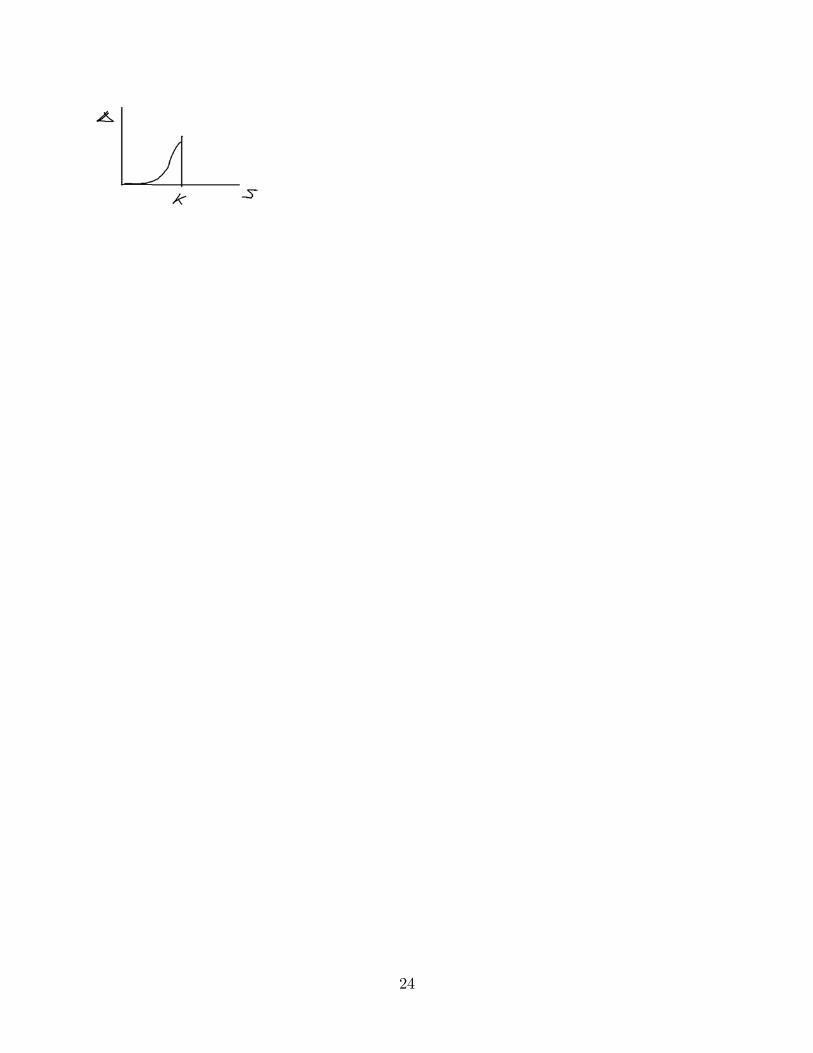
¶22

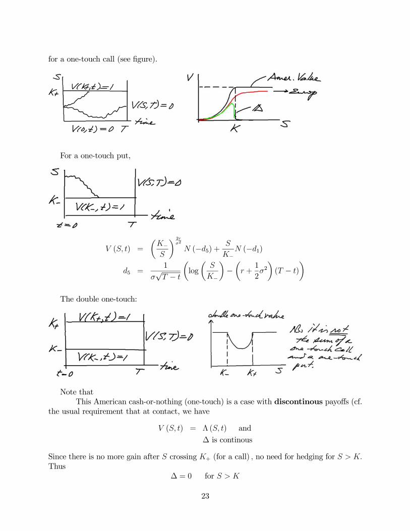
for a one-touch call (see figure).

For a one-touch put,

V (S, t) =

µK−S

¶ 2rσ2

N (−d5) + S

K−N (−d1)

d5 =1

σ√T − t

µlog

µS

K−

¶−µr +

1

2σ2¶(T − t)

¶

The double one-touch:

Note thatThis American cash-or-nothing (one-touch) is a case with discontinous payoffs (cf.

the usual requirement that at contact, we have

V (S, t) = Λ (S, t) and

∆ is continous

Since there is no more gain after S crossing K+ (for a call) , no need for hedging for S > K.Thus

∆ = 0 for S > K

23

24