Contents

1 ANOVA 21.1 Completely randomized One-Way ANOVA . . . . . . . . . . . . . . . . . . . . . . . . 21.2 The extra sum of square principle . . . . . . . . . . . . . . . . . . . . . . . . . . . . . 81.3 Testing for Equality of All Treatment Means . . . . . . . . . . . . . . . . . . . . . . . 91.4 Estimating and Testing Differences in Treatment Means . . . . . . . . . . . . . . . . . 141.5 Multiple Comparisons . . . . . . . . . . . . . . . . . . . . . . . . . . . . . . . . . . . 191.6 Residual Analysis - Checking the Assumptions . . . . . . . . . . . . . . . . . . . . . . 23

2 Extra ANOVA Example 252.1 The example . . . . . . . . . . . . . . . . . . . . . . . . . . . . . . . . . . . . . . . . . 252.2 F-test . . . . . . . . . . . . . . . . . . . . . . . . . . . . . . . . . . . . . . . . . . . . 252.3 Multiple comparison . . . . . . . . . . . . . . . . . . . . . . . . . . . . . . . . . . . . 262.4 Contrast . . . . . . . . . . . . . . . . . . . . . . . . . . . . . . . . . . . . . . . . . . . 26

1

1 ANOVA

ANOVA means ANalysis Of VAriance.The ANOVA is a tool for studying the influence of one or more qualitative variables on the mean ofa numerical variable in a population.

In ANOVA the response variable is numerical and the explanatory variables are cate-gorical.

Example: A local school board is interested in comparing test scores on a standardized reading testfor fourth–grade students in their district. They select a random sample of children from each ofthe local elementary schools. Since it is known that reading scores vary at that age from males tofemales, they use an analysis, which can tell them if there is a difference in those scores between theschools correcting for the influential factor gender.Response variable: reading score (numerical)Factor variables: gender and the elementary school the student is attending (factors are categorical).Level of gender are male/female

One possible treatment would be ”male from Rideau Park School”

We would analyze if the mean reading score depends on the categorical variables ”Sex” and ”School”.

Definition:

� The response variable(dependent variable) is the variable of interest to be measured in theexperiment.

� Factors are the variables whose effect on the response variable is studied in the experiment.

� Factor levels are the values of a factor in the experiment.

� Treatments are the possible factor level combinations in the experiment. (One factor level foreach factor is combined with factor level from other factors)

� A designed experiment is an experiment in which the researcher chooses the treatments to beanalyzed and the method for assigning individuals to treatments.

1.1 Completely randomized One-Way ANOVA

We will start with revisiting the One-Way-ANOVA model which you might have seen in the previouscourse.In Completely Randomized One-way ANOVA ”one-way” indicates that only one factor is consideredand ”completely randomized” indicates that the experimental units are assumed to be randomlyassigned to the factor levels, or have been randomly sampled within each factor level.

Example 1Where shall we stay for our trip to the mountains in Reading Week?Is the mean fee charged for one night in an AirBnB property accommodating at least 6 adults differfor Jasper, Banff and Canmore?

2

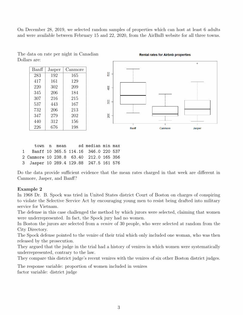
On December 28, 2019, we selected random samples of properties which can host at least 6 adultsand were available between February 15 and 22, 2020, from the AirBnB website for all three towns.

The data on rate per night in CanadianDollars are:

Banff Jasper Canmore283 192 165417 161 129220 302 209345 206 184307 216 215537 443 167732 206 213347 279 202440 312 156226 676 198

town n mean sd median min max

1 Banff 10 365.5 114.16 346.0 220 537

2 Canmore 10 238.8 63.40 212.0 165 356

3 Jasper 10 289.4 129.88 247.5 161 576

Do the data provide sufficient evidence that the mean rates charged in that week are different inCanmore, Jasper, and Banff?

Example 2In 1968 Dr. B. Spock was tried in United States district Court of Boston on charges of conspiringto violate the Selective Service Act by encouraging young men to resist being drafted into militaryservice for Vietnam.The defense in this case challenged the method by which jurors were selected, claiming that womenwere underrepresented. In fact, the Spock jury had no women.In Boston the jurors are selected from a venire of 30 people, who were selected at random from theCity Directory.The Spock defense pointed to the venire of their trial which only included one woman, who was thenreleased by the prosecution.They argued that the judge in the trial had a history of venires in which women were systematicallyunderrepresented, contrary to the law.They compare this district judge’s recent venires with the venires of six other Boston district judges.

The response variable: proportion of women included in veniresfactor variable: district judge

3

The data:judge Statistic valueA Mean 34.1200

Std. Deviation 11.94182Sample Size 5

B Mean 33.6167Std. Deviation 6.58222

Sample Size 6C Mean 29.1000

Std. Deviation 4.59293Sample Size 9

D Mean 27.0000Std. Deviation 3.81838

Sample Size 2E Mean 26.9667

Std. Deviation 9.01014Sample Size 6

F Mean 26.8000Std. Deviation 5.96888

Sample Size 9Spock Mean 14.6222

Std. Deviation 5.03879Sample Size 9

The question to be explored, if the factor variable (the treatment) has an impact on the meanresponse variable, or is the mean of the response variable different for the different treatments. (Isthe data indicating that the mean proportion of women in venires differs for the different judges).

The Model:It is assumed that the population is normally distributed, but that the means of the experimentalunits depend on the treatment.Let k be the number of different treatments (this would be 7 for the Spock data) and letxij be the j-th measurement of the response variable for treatment i, (the proportion of women onthe j-th venire for judge i) then assume that

xij = µi + eij

where µi is the mean of the response variable for experimental units with treated with treatment i,andeij is the error in this measurement, or the part in the measurement that can not be explainedthrough the treatment.It is assumed that the error is normally distributed with mean zero and standard deviation σ.(eij ∼ N (0, σ))This statement includes a very strong assumption: The standard deviation is the same for all treat-ments, which is similar to the assumption of equal standard deviation for the pooled t-test.

In this model the population is described through k potentially different means.Since we want to see if the treatment impacts the mean of the response variable, the null hypothesisof the test of interest is

4

H0 : µ1 = µ2 = . . . = µk vs. Ha: at least one of the means is different from the others.

The arguments underlying an ANOVAEvery experiment results in data, that brings in a certain amount of variability (variance).In an ANOVA the total variance is divided into portions that can be attributed to the differentfactors of interest.

The analysis of these portions will show the effect of the factors on the response.

Example:Consider data from two different populations A and B:

Set A

a a a b b b

----------------------------------------

Set B

a b a b a b

-----------------------------------------

The total variance in the two data sets is almost the same, but for set A the variability withinthe groups is much less than in set B.

Set ASince the variance in the groups in relationship to the total variance is relatively small, thetotal variance can only be explained by the variance (difference) between the groups, so that onewould conclude that the means for the groups must be different.

Set BThe variance of the groups is close to the total variance, so that the total variance is explained bythis variance. One concludes that the variance between the groups can’t be large, so that the meansin the groups might not be different.

ANOVA is based on the comparison of the variance of the sample means with the variancewithin the k samples.The calculation of the variances are all based onsum of squares.

The different sum of squares in a one way ANOVA:

TotalSS: The total variance in the experiment, is the variance of the combined k samples. It is based on

the total sum of squares

TotalSS =∑

(xij − x)2 =∑

x2ij −

(∑xij)

2

n

where x is the overall mean, from all k samples and n = n1 + n2 + . . .+ nk.

In ANOVA we analyze the total variance. In one way ANOVA part of the variance can beexplained through the use the different treatments and the leftover of the variance must thenbe due to error in the measurements (or other factors not included in the model).

5

SST : The variance explained through the treatment is based on the sum of squares for treatment(SST ), it measures the variation among the k sample means (from one sample to the others):

SST =∑

ni(xi − x)2

SSE: The variance explained through the error in the measurements is based on the sum of squaresfor error (SSE), it is also used to estimate the variation within the k samples:

SSE = (n1 − 1)s21 + (n2 − 1)s2

2 + . . .+ (nk − 1)s2k

Assuming the standard deviations in all k populations are the same, than this is an estimatefor the variation inside the populations which is the variance from the model, σ2.

It is possible to proof algebraically, that always

TotalSS = SST + SSE

Therefore, it is only necessary to calculate two of the sum of squares and find the third one with thislast identity.

Each of the sum of squares, when divided by its appropriate degrees of freedom, provides an esti-mate of the total variance in all measurements and the variances due to treatment and error in theexperiment.

dfTotal: Since TotalSS involves n squares its degrees of freedom are df = n− 1.

dfT : Since SST involves k squares its degrees of freedom are df = k − 1.

dfE: Since SSE involves (n1 − 1) + (n2 − 1) + . . .+ (nk − 1) = n− k squares its degrees of freedomare df = n− k.

Observe that also for the degrees of freedom the identity holds that

df(TotalSS) = df(SST ) + df(SSE)

Mean squares (MS) are calculated by dividing the sum of squares by their degrees of freedomMS = SS/df . All the results are displayed in an ANOVA table:

ANOVA Table for k independent Random Samples

Source df SS MS FTreatments k − 1 SST MST = SST/(k − 1) MST/MSEError n− k SSE MSE = SSE/(n− k)Total n− 1 TotalSS

With

F :=MST

MSE

6

the variation due to the Error is compared with the variation due to the treatment. If the variationdue to the treatment is much larger than the variation due to the Error (i.e. F is large), the dataindicate that the treatment has an effect on the mean response.

Continue AirBnB example:From the summary statistics obtain SSE and SST :

SSE = (n1 − 1)s21 + (n2 − 1)s2

2 + . . .+ (nk − 1)s2k

= (10− 1)114.162 + (10− 1)63.402 + (10− 1)129.882

= 305276

and

x =n1x1 + n2x2 + . . .+ nkxk

n1 + n2 + . . .+ nk=

8937

30= 297.9

That gives

SST =∑

ni(xi − x)2

= 10(365.5− 297.9)2 + 10(238.8− 297.9)2 + 10(289.4− 297.9)2

= 81348

and

TotalSS = SST + SSE = 386624

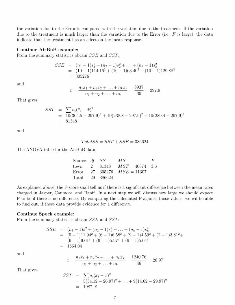
The ANOVA table for the AirBnB data:

Source df SS MS Ftown 2 81348 MST = 40674 3.6Error 27 305276 MSE = 11307Total 29 386624

As explained above, the F-score shall tell us if there is a significant difference between the mean ratescharged in Jasper, Canmore, and Banff. In a next step we will discuss how large we should expectF to be if there is no difference. By comparing the calculated F against those values, we wil be ableto find out, if these data provide evidence for a difference.

Continue Spock example:From the summary statistics obtain SSE and SST :

SSE = (n1 − 1)s21 + (n2 − 1)s2

2 + . . .+ (nk − 1)s2k

= (5− 1)11.942 + (6− 1)6.582 + (9− 1)4.592 + (2− 1)3.812+(6− 1)9.012 + (9− 1)5.972 + (9− 1)5.042

= 1864.04

and

x =n1x1 + n2x2 + . . .+ nkxk

n1 + n2 + . . .+ nk=

1240.76

46= 26.97

That givesSST =

∑ni(xi − x)2

= 5(34.12− 26.97)2 + . . .+ 9(14.62− 29.97)2

= 1987.91

7

and

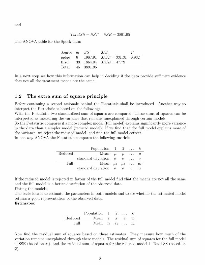
TotalSS = SST + SSE = 3891.95

The ANOVA table for the Spock data:

Source df SS MS Fjudge 6 1987.91 MST = 331.31 6.932Error 39 1864.04 MSE = 47.79Total 45 3891.95

In a next step see how this information can help in deciding if the data provide sufficient evidencethat not all the treatment means are the same.

1.2 The extra sum of square principle

Before continuing a second rationale behind the F-statistic shall be introduced. Another way tointerpret the F-statistic is based on the following:With the F statistic two standardized sum of squares are compared. These sums of squares can beinterpreted as measuring the variance that remains unexplained through certain models.So the F-statistic compares if a more complex model (full model) explains significantly more variancein the data than a simpler model (reduced model). If we find that the full model explains more ofthe variance, we reject the reduced model, and find the full model correct.In one way ANOVA the F-statistic compares the following models

Population 1 2 . . . kReduced Mean µ µ . . . µ

standard deviation σ σ . . . σFull Mean µ1 µ2 . . . µk

standard deviation σ σ . . . σ

If the reduced model is rejected in favour of the full model find that the means are not all the sameand the full model is a better description of the observed data.Fitting the models:The basic idea is to estimate the parameters in both models and to see whether the estimated modelreturns a good representation of the observed data.Estimates:

Population 1 2 . . . kReduced Mean x x x x

Full Mean x1 x2 . . . xk

Now find the residual sum of squares based on these estimates. They measure how much of thevariation remains unexplained through these models. The residual sum of squares for the full modelis SSE (based on xi), and the residual sum of squares for the reduced model is Total SS (based onx).

8

The F-statistic shows how much more variation is explained through the full model (after standard-ization) than through the reduced model,

F =(Total SS − SSE)/dfT

SSE/dfE

If F is large it indicates that the full model is significantly superior to the reduced model in describingthe observed data, and it is decided that the full model should be adopted.

As mentioned above the goal is to use a 1-way ANOVA for the analysis of the means of differentpopulations µ1, µ2, . . . , µk. In a next step we now want to use the information from the ANOVAtable, to test hypotheses and give confidence intervals concerning those population means.

1.3 Testing for Equality of All Treatment Means

The hypotheses of interest are

H0 : µ1 = µ2 = . . . = µk versus Ha : at least one of the means differs from the others

Use the following argument for developing the test:

� Remember that that the variances in the k populations are assumed to be all the same σ2. Thestatistic

MSE =SSE

n− kis a pooled estimate of σ2 (a weighted average of all k sample variances), whether or not H0 istrue.

� If H0 is true, then the variation in the sample means, measured by

MST =SSG

k − 1

also provides an unbiased estimate of σ2, this is derived from σ2x = σ2/n.

However, if H0 is false and the population means are not the same, then MST is larger thanσ2.

� The test statistic

F =MST

MSE

tends to be much larger than 1, if H0 is false. Hence, H0 can be rejected for large values of F .

What values of F have to be considered large, we learn from the distribution of F .

� If H0 is true, the statistic

F =MST

MSE

has an F distribution with df1 = (k − 1) and df2 = (n− k) degrees of freedom.

Upper tailed critical values of the F distribution can be found in Table VIII-XI

9

The ANOVA F-Test

1. The Hypotheses are

H0 : µ1 = µ2 = . . . = µk versusHa : at least one of the means differs from the others

2. Assumption: The population follows a normal distribution with means µ1, µ2, . . . , µk and equalvariance σ2. The samples are independent random samples from each population.

3. Test statistic:

F0 =MST

MSE

based on df1 = (k − 1) and df2 = (n− k).

4. P-value: P (F > F0), where F follows an F -distribution with df1 = (k − 1) and df2 = (n− k).

5. Decision:If P-value≤ α, then reject H0.If P-value> α, then do not reject H0.

6. Put into context.

Continue AirBnB example:The data on rental rates of AirBnB properties in Jasper, Banff, and Canmore resulted in the followingANOVA table

Source df SS MS Ftown 2 81348 MST = 40674 3.6Error 27 305276 MSE = 11307Total 29 386624

Use this information now to test if the data provide sufficient evidence that the mean rates in thethree towns are hot all the same during Reading Week in 2020.Conduct an ANOVA F-test:

1. Hypotheses: Let µi=mean rate charged for one night in an AirBnB property suitable for atleast 6 adults in Reading Week in town i.

H0 : µJ = µC = µB versusHa : at least one of the means differs from the others

choose α = 0.05

2. The samples can be considered random samples. The box plots all look reasonable symmetricand do not provide strong evidence against the assumption of normality. The standard devia-tions are close enough to each other to be not of concern of violating the assumption of equalvariances in the subgroups.

3. Test statistic: (from ANOVA table)

F0 = 3.6 with dfn = 2, dfd = 27

10

4. P-value: The P-value is the uppertail area for F0 = 3.6

Use the table for the F-distribution, find dfn = 2 and dfd = 27 .

F0 = 3.6 falls between critical values for α = 0.05 and α = 0.025, and we conclude that0.025 <P-value < 0.05

5. Decision: The P-value< 0.005 < 0.05 = α, we reject H0.

6. Put into context:At significance level 0.05 the data provide sufficient evidence that the mean rental rates forAirBnB properties for at least six guests in Banff, Jasper, and Canmore are not all the samein the 2020 Reading Week.

The question arising out of this answer is: Where are the (significant) differences?

Continue Spock example:The data resulted in the following ANOVA table:

Source df SS MS Fjudge 6 1987.91 MST = 331.31 6.932Error 39 1864.04 MSE = 47.79Total 45 3891.95

Conduct an ANOVA F-test:

1. Hypotheses: Let µi=mean proportion of women on a venire for judge i.

H0 : µA = µB = µC = µD = µE = µF = µSpock versusHa : at least one of the means differs from the others

choose α = 0.05

2. According to the box plot the data can be assumed to be normal (all boxes are pretty sym-metric). Only for one judge we find the standard deviation much higher than for the others,this could cause problems.

3. Test statistic:F0 = 6.932 with dfn = 6, dfd = 39

4. P-value: The P-value is the uppertail area for F0 = 6.932

Use the table for the F-distribution, find df1 = 6 and df2 = 30 (largest df in the table smallerthan 39).

6.932 is larger than the largest value in the block of values for this particular choice of df, whichis 3.95. Therefore the P-value is smaller than 0.005, the upper tail area for 3.95.

State: P-value< 0.005.

11

5. Decision: The P-value< 0.005 < 0.05 = α, we reject H0.

6. Put into context:At significance level 0.05 the data provide sufficient evidence that at least for one judge themean proportion of women on venires is different from the mean proportion of the other judges.

The test above indicates that the mean proportion of women are not the same for all judges. Thenext task would be to find out where out where the differences can be found.

Example 3Sevoflurane and Desflurane Concentration in Post-Anesthesia Care Units (PACUs).

According to Wikipedia desflurane is a highly fluorinated methyl ethyl ether used for maintenanceof general anesthesia, and sevoflurane is a sweet-smelling, nonflammable, highly fluorinated methylisopropyl ether used as an inhalational anaesthetic for induction and maintenance of general anes-thesia. Both are commonly used volatile anesthetic agents used during surgeries. Both are usuallyconsidered safe for anesthesia but are recognized as occupational hazard for health professionals. Astudy aimed to document and investigate differences in desflurane and sevoflurane concentrations inthe breath of nurses in pediatric PACUs and adult PACUs. The study also included a control groupof residents, who were not exposed to the agents in the previous 3 month.For all participants measurements indicating the concentration of desflurane and sevoflurane weretaken in the morning. Nurses were about to start a day shift (after they had worked the day beforethe same shift).Do the data indicate that there are differences in the mean concentration of desflurane concentrationin the breath between the three groups (pediatric, adult, control)?

Group n mean st.dev.Pediatric 10 1.74 0.417Adult 10 1.77 0.416Control 10 1.21 0.213

From the summary statistics obtain SSE and SST :

SSE = (n1 − 1)s21 + (n2 − 1)s2

2 + (n3 − 1)s23

= (10− 1)0.4172 + (10− 1)0.4162 + (10− 1)0.2132

= 3.5308

and

x =n1x1 + n2x2 + n3x3

n1 + n2 + n3

=47.2

30= 1.573

That givesSST =

∑ni(xi − x)2

= 10(1.74− 1.573)2 + 10(1.77− 1.573)2 + 10(1.21− 1.573)2

= 1.98467

and

TotalSS = SST + SSE = 5.51547

Producing the following ANOVA table for desflurane

12

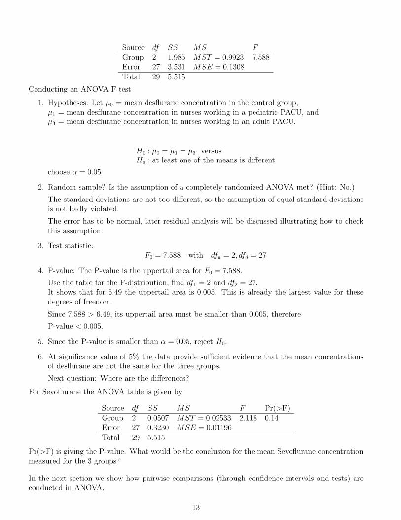
Source df SS MS FGroup 2 1.985 MST = 0.9923 7.588Error 27 3.531 MSE = 0.1308Total 29 5.515

Conducting an ANOVA F-test

1. Hypotheses: Let µ0 = mean desflurane concentration in the control group,µ1 = mean desflurane concentration in nurses working in a pediatric PACU, andµ3 = mean desflurane concentration in nurses working in an adult PACU.

H0 : µ0 = µ1 = µ3 versusHa : at least one of the means is different

choose α = 0.05

2. Random sample? Is the assumption of a completely randomized ANOVA met? (Hint: No.)

The standard deviations are not too different, so the assumption of equal standard deviationsis not badly violated.

The error has to be normal, later residual analysis will be discussed illustrating how to checkthis assumption.

3. Test statistic:F0 = 7.588 with dfn = 2, dfd = 27

4. P-value: The P-value is the uppertail area for F0 = 7.588.

Use the table for the F-distribution, find df1 = 2 and df2 = 27.It shows that for 6.49 the uppertail area is 0.005. This is already the largest value for thesedegrees of freedom.

Since 7.588 > 6.49, its uppertail area must be smaller than 0.005, therefore

P-value < 0.005.

5. Since the P-value is smaller than α = 0.05, reject H0.

6. At significance value of 5% the data provide sufficient evidence that the mean concentrationsof desflurane are not the same for the three groups.

Next question: Where are the differences?

For Sevoflurane the ANOVA table is given by

Source df SS MS F Pr(>F)Group 2 0.0507 MST = 0.02533 2.118 0.14Error 27 0.3230 MSE = 0.01196Total 29 5.515

Pr(>F) is giving the P-value. What would be the conclusion for the mean Sevoflurane concentrationmeasured for the 3 groups?

In the next section we show how pairwise comparisons (through confidence intervals and tests) areconducted in ANOVA.

13

1.4 Estimating and Testing Differences in Treatment Means

Is the ANOVA F-test significant, one can conclude at the given significance level that not all popu-lation means are the same, but through this test we can not determine where the differences occur.In order to locate the differences pairwise comparisons should be conducted, i.e. look at parametersµ1 − µ2, . . . , µ1 − µkµ2 − µ3, . . . , µ2 − µk. . .µk−1 − µk

There is a total of k(k − 1)/2 parameters for pairwise comparisons of k means.The comparisons can be done with the help of t-tests or t-CIs.

For some studies the pairwise comparisons are not the main focus, like in the Spock example; hereit is more relevant to compare µSpock with the average of all the other means

µ =µA + µB + µC + µD + µE + µF

6

The parameter of interest in that case would be

1

6µA +

1

6µB +

1

6µC +

1

6µD +

1

6µE +

1

6µF − µSpock

For the study on the concentration of volatile anesthetic agents in the breath in a control groupversus nurses working in pediatric and adult PACUs one might be really interested in comparing thetwo groups of nurses with the control group reflected in

1

2(µP + µA)− µC =

1

2µP +

1

2µA − µC

When comparing the rates payable for staying one night in an AirBnB we might be more interestedin comparing the prices between options for Banff National Park (Banff and Canmore) versus JasperNational Park (Jasper), so we compare the mean rate paid in Jasper, µJ , with the average of themean rates paid in Banff and in Canmore, 1/2(µB + µC). resulting in the contrast

γ = µJ −1

2(µB + µC) = 1 · µJ + (−1

2) · µB + (−1

2) · µC

In order to describe this family of parameters of interest we look at contrasts.

Contrasts:Linear combinations of the group means have the form

γ = C1µ1 + C2µ2 + . . .+ Ckµk

If the coefficients add to zero (C1 + C2 + . . .+ Ck = 0) the linear combination is called a contrast.

14

Example 4For pairwise comparisons the linear combinations is

γ = µ1 − µ2 = 1µ1 + (−1)µ2 + 0µ3 + . . .+ 0µk

with C1 = 1, C2 = −1, C3 = . . . = Ck = 0. Since these total to zero a pairwise comparison leads to acontrast.

The linear combination for the Spock example is

γ =1

6µA +

1

6µB +

1

6µC +

1

6µD +

1

6µE +

1

6µF − µSpock,

which gives CA = CB = . . . = CF = 1/6 and CSpock = −1, with a total CA + . . . + CF + CSpock = 0,so it is a contrast.

For the anesthesia example it would be

γ =1

2µP +

1

2µA − µC

with CP = CA = 1/2 and CC = −1, with a total CP + CA + CC = 0, so it is a contrast.

The AirBnB example results in the contrast

γ = µJ −1

2(µB + µC) = 1 · µJ + (−1

2) · µB + (−1

2) · µC

A contrast γ becomes the unknown population parameter. How can this parameter be estimatedfrom the available data?

The sample contrast estimating γ = C1µ1 + C2µ2 + . . .+ Ckµk is

c = C1x1 + C2x2 + . . .+ Ckxk

To find a confidence interval for γ, we study the distribution of c. c is based on a random sampletherefore assumes random values, it is a random variable and therefore is described by a distribution.For the distribution of c one finds

µc = γ, SE(c) = sp

√C2

1

n1

+C2

2

n2

+ . . .+C2k

nk

where sp =√MSE

So c is an unbiased estimator for γ (why?).From this we conclude

t =c− γSE(c)

has a t-distribution with df = n− k.From this we derive the

(1− α)100% Confidence Interval for γ

c± tdf1−α/2SE(c)

tdf1−α/2 is the 1− α/2 percentile of the t-distribution with df = n− k.

15

t-test for contrasts

1. Hypotheses:H0 : γ = 0 versus Ha : γ 6= 0H0 : γ ≤ 0 versus Ha : γ > 0H0 : γ ≥ 0 versus Ha : γ < 0

2. Assumption: Random samples, the response variable is normally distributed, and the standarddeviation is the same for all treatments.

3. Test Statistic:

t0 =c

SE(c), df = n− k

4. P-value:Hypotheses P-valuetwo-tailed 2P (t > abs(t0))upper-tailed P (t > t0)lower-tailed P (t < t0)

5. Decision:P-value≤ α, then reject H0 P-value> α, then do not reject H0

Application: A confidence interval for comparing two means within the ANOVA model is then:(1− α)100% Confidence interval for µi − µj:

(xi − xj)± tα/2

√√√√s2p

(1

ni+

1

nj

)

with s2p = MSE and tα/2 the (1− α/2) percentile of the t-distribution with df = n− k.

Continue AirBnB Example: Find confidence intervals for all pairwise comparisons:

1. γ = µJ − µC = 1 · µJ + (−1) · µC + 0 · µB : c = 1 · xJ + (−1) · xC + 0 · xB = xJ − xC2. γ = µJ − µB = 1 · µJ + 0 · µC + (−1) · µB : c = 1 · xJ + 0 · xC + (−1) · xB = xJ − xB3. γ = µC − µB = 0 · µJ + 1 · µC + (−1) · µB : c = 0 · xJ + 1 · xC + (−1) · xB = xC − xB

Since the sample sizes are all the same SE(c) are the same for all three confidence intervals

SE(c) = sp

√(1)2

10+

(−1)2

10,with sp =

√MSE =

√11307 = 106.33

such that SE(c) = 47.55, using the t-critical value (for a 95% confidence interval) t270.025 = 2.052 (from

the t-table), one finds that the margin of error for all confidence intervals is 2.052(47.55) = 97.58The confidence intervals are therefore:

1. (289.4− 238.8)± 97.58 : c = 50.6 : [−46.98, 148.18]2. (289.4− 365.5)± 97.58 : c = −76.11 : [−173.68, 21.48]3. (238.8− 365.5)± 97.58 : c = −126.7 : [−224.28,−29.12]

16

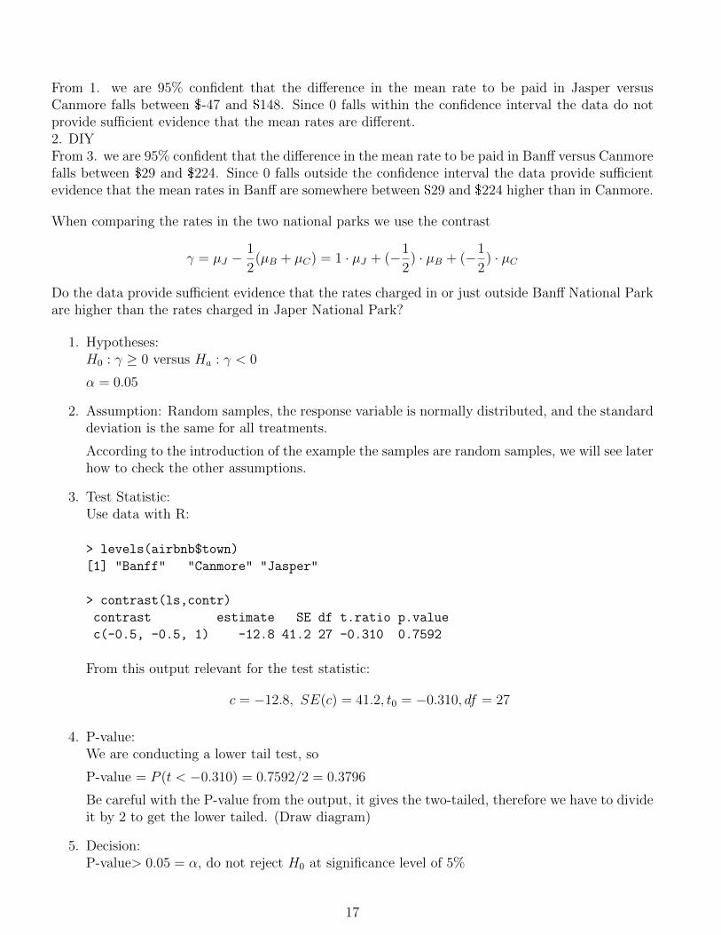
From 1. we are 95% confident that the difference in the mean rate to be paid in Jasper versusCanmore falls between $-47 and $148. Since 0 falls within the confidence interval the data do notprovide sufficient evidence that the mean rates are different.2. DIYFrom 3. we are 95% confident that the difference in the mean rate to be paid in Banff versus Canmorefalls between $29 and $224. Since 0 falls outside the confidence interval the data provide sufficientevidence that the mean rates in Banff are somewhere between $29 and $224 higher than in Canmore.

When comparing the rates in the two national parks we use the contrast

γ = µJ −1

2(µB + µC) = 1 · µJ + (−1

2) · µB + (−1

2) · µC

Do the data provide sufficient evidence that the rates charged in or just outside Banff National Parkare higher than the rates charged in Japer National Park?

1. Hypotheses:H0 : γ ≥ 0 versus Ha : γ < 0

α = 0.05

2. Assumption: Random samples, the response variable is normally distributed, and the standarddeviation is the same for all treatments.

According to the introduction of the example the samples are random samples, we will see laterhow to check the other assumptions.

3. Test Statistic:Use data with R:

> levels(airbnb$town)

[1] "Banff" "Canmore" "Jasper"

> contrast(ls,contr)

contrast estimate SE df t.ratio p.value

c(-0.5, -0.5, 1) -12.8 41.2 27 -0.310 0.7592

From this output relevant for the test statistic:

c = −12.8, SE(c) = 41.2, t0 = −0.310, df = 27

4. P-value:We are conducting a lower tail test, so

P-value = P (t < −0.310) = 0.7592/2 = 0.3796

Be careful with the P-value from the output, it gives the two-tailed, therefore we have to divideit by 2 to get the lower tailed. (Draw diagram)

5. Decision:P-value> 0.05 = α, do not reject H0 at significance level of 5%

17

6. Context:At significance level of 5% the data do not provide sufficient evidence that the mean ratecharged for AirBnB properties suitable for at least 6 people in Reading Week is significantlyhigher in Banff National Park than in Jasper National Park.

Continue Spock Example: We obtain 95% confidence intervals for µA − µSpock, µB − µSpock,µC − µSpock, µD − µSpock,µE − µSpock, and µE − µSpock, in order to figure out if the mean on µSpock issignificant different from all the other means.

µA − µSpock:For γ = µA − µSpock CA = 1, CSpock = −1 and all others are 0.

c = xA − xSpock, SE(c) = sp

√√√√(1)2

nA+

(−1)2

nSpock= sp

√1

5+

1

9

t390.975 = 2.023, so we get

(34.12− 14.62)± 2.023 · 6.89√

15

+ 19

19.5± 7.775(11.73 ; 27.27)

in the same way we get95% CI

µB − µSpock (11.5848 26.4152)µC − µSpock (7.8476 21.1124)µD − µSpock (1.3815 23.3785)µE − µSpock (4.9348 19.7652)µF − µSpock (5.5476 18.8124)

None of the confidence intervals captures zero, we are 95% confident that the mean proportion ofwomen on venires for any judge and Spock’s judge are different (95% confident for each interval).We are looking at 6 confidence interval every single CI has a 95% chance of capturing the parameterof interest. But there is also the chance that any of them does not capture the parameter we arelooking for. And when looking at the whole set of CIs, it is likely that we miss at least one ofthe parameters with the six intervals. This is an undesirable effect of conducting many differentcomparisons.The other CI we are interested in is a 95%CI for γ = 1

6µA + 1

6µB + 1

6µC + 1

6µD + 1

6µE + 1

6µF −µSpock:

(29.6− 14.62)± 2.042 · 6.89

√1

62 · 5+

1

62 · 6+

1

62 · 9+

1

62 · 2+

1

62 · 6+

1

62 · 9+

(−1)2

9

14.98± 2.042 · 6.89 · 0.382 = [9.61, 20.35]

Since zero is not included with the interval we are 95% confident, that the mean proportion of womenon venires from Spock’s judge is significant lower than the mean for all the other 6 judges.

Continue Desflurane Example:Test if the mean desflurane concentration is in the morning higher for nurses working in PACUs thanin the control group.Choose γ = 1

2(µP + µA)− µC .

t-test for contrasts

18

1. Hypotheses: H0 : γ ≤ 0 versus Ha : γ > 0

2. Assumption: Addressed these when doing the ANOVA

3. Test Statistic:c = 1

2(1.74 + 1.77)− 1.21 = 0.545, sp =

√MSE = 0.362,

SE(c) = 0.362

√0.52

10+

0.52

10+

(−1)2

10= 0.1402

and

t0 =0.545

0.1402= 3.628, df = 27

4. P-value: Upper tailed test (Ha : γ > 0), P-value = P (t > 3.628) In table IV use df=27, andfind that P-value<0.005.

5. Decision: P-value< α = 0.05, reject H0

6. At significance level of 5% the data provide sufficient evidence that the mean concentration ofdesflurane is higher for nurses working in PACUs then in the control group.

1.5 Multiple Comparisons

As mentioned above, when simultaneously conducting several comparisons (confidence intervals,tests) at significance level of α, the probability that one of the results in the overall statement iswrong can be much higher than α. The more comparisons are made the more likely it becomes thatat least one decision is wrong, i.e. the overall error probability increases with every extra comparisonincluded with the overall statement.This effect is problematic, because we already have to accept that in inferential statistics we mightmake mistakes. This was found acceptable as long as the probability for making an error was knownand could be chosen (α). This control is lost when making multiple comparisons without takingthe described effect into account. In order to counteract the effect different strategies have beendeveloped to control the overall or experiment wise (versus comparison wise) error rate in multiplecomparisons.

Different multiple comparison methods

1. Tukey-HSD (honest significant difference) procedure:Can only be used when it is required to investigate ALL pairwise comparisons of several means.Since taking advantage of this special situation the CIs are narrower than for the other methods,when it can be used.

2. Bonferroni method:Can be used in very general situation where we want to control the overall error rate of amultiple comparison, it usually low power.

For the Bonferroni method, only α for the t-CI has to be adjusted: When doing m pairwisecomparisons, then choose α∗ = α/m for each comparison.

19

3. Scheffe method:Can be used also for multiple contrasts, but will result in wider CIs than Tukey if applied topairwise comparisons.

Conducting a multiple comparison using Bonferroni’s method

1. Choose the acceptable experiment wise error rate, α.

2. Find m= the number of comparisons you want to make.

3. Calculate α∗ = α/m the comparison wise error rate

4. Rank the sample means from the samples of those populations you want to compare fromsmallest to largest

5. Determine the margin of error (ME) for each comparison (µi − µj)

MEij = tn−kα∗/2

√MSE

√1

ni+

1

nj

6. Place a bar under those pairs of treatments that differ less than the margin of error. A pair oftreatments not connected by a bar implies a difference in the population means.

The confidence level associated with all statements at once is at least (1− α).

Continue AirBnB example:

1. α = 0.05.

2. m = 3(3− 1)/2 = 3 is the number of comparisons (muJ − µB, µJ − µC , µB −muC).

3. α∗ = α/3 = 0.01666 the comparison wise error rate.

4.

xC < xJ < xB238.8 289.4 365.5

5. The margin of error (ME) is the same for all three comparisons because the sample sizes areall the same.

ME = t270.008(106.33)

√1

10+

1

10= 131.77

with t270.008 ≈ 2.771 from table IV.

6. xJ − xC = 50.6 < ME, underline xJ and xCxB − xC = 126.7 < ME, continue line to xBxB − xJ = 76.1 < ME

xC < xJ < xB238.8 289.4 365.5—————————-

20

7. At experimentwise error rate of 5% the data do not indicate any significant pairwise differencesbetween the mean rates for AirBnB properties housing at least 6 people in Reading Week 2002

This is odd, since the F-test said there is at least one difference, but this method is no sensitiveenough to detect where the difference is.

Example 5Spock’s example using the Bonferroni method

1. α = 5%

2. m = 7(6)/2 = 21

3. α∗ = 0.05/21 = 0.00238

4. the ranked means are

14.62, 26.80, 26.97, 27.00, 29.10, 33.62, 34.12

5. For the percentile find α∗/2 ≈ 0.001 for df = 39 use t390.001 = 3.31 (from online calculator - the

best we can get from the table is t390.005 = 2.708)

This gives the following margin of errors for the different comparisons

Judge/sample sizeSpock’s A B C D E F

9 5 6 9 2 6 9Spock’s 9 13.05 12.33 11.03 18.29 12.33 11.03

A 5 14.17 13.05 19.57 14.17 13.05B 6 12.33 19.11 13.51 12.33C 9 18.29 12.33 11.03D 2 19.11 18.29E 6 12.33F 9

6. If we put the bars on, we get

14.62 26.80 26.97 27.00 29.10 33.62 34.12

Spock’s F E D C B A

------- -------

----------------------------------------------------

In conclusion we find at 95% confidence that the mean proportion of women on venires is significantlydifferent for Spock’s judge and judges besides F, E, C, B and A. The mean proportion of women onvenires for judges F-A do not differ significantly.The mean proportion of women on venires from Spock’s judge and judge D do not differ significantly.But judge D is special because only two of his venires were included in the study resulting in a verylarge standard error, which in conclusion is not significantly different from any other judge.

21

Example 6Compare the mean desflurane concentration for the three groups.

1. α = 0.05.

2. m = 3(3− 1)/2 = 3 is the number of comparisons (mu0 − µ1, µ0 − µ3, µ1 −mu3).

3. α∗ = α/3 = 0.01666 the comparison wise error rate.

4.

x0 < x1 < x3

1.21 1.74 1.77

5. The margin of error (ME) is the same for all three comparisons because the sample sizes areall the same.

ME = t270.008(0.362)

√1

10+

1

10= 0.4486

with t270.008 ≈ 2.771 from table IV.

6. x3 − x0 = 0.56 > MEx3 − x1 = 0.03 < ME, underline x1 and x3

x1 − x0 = 0.53 > ME

x0 < x1 < x3

1.21 1.74 1.77————–

7. At experimentwise error rate of 5% the data provide sufficient evidence that the mean con-centration of desflurane in the breath in the control group is significant lower than for bothpediatric and adult PACU nurses in the morning after a shift on the day before. The analysisdid not show a significant difference when comparing the mean concentration for pediatric andadult PACU nurses.

22

1.6 Residual Analysis - Checking the Assumptions

The assumptions for all the tests in ANOVA can be written as:

1. Samples are random samples

2. The model is an appropriate description of the population

To understand what needs to be checked reconsider the one-way ANOVA model:

xij = µi + eij, eij ∼ N (0, σ)

The model implies that observations can be viewed as treatment mean plus some error, where theerror comes from a normal distribution with mean 0 and common standard deviation, σ.

In order to check this assumption we focus on the error, which we will check for normality andhomoscedasticity.To do this we first need to extract the error from the measurements which leads us to the residuals.For one way ANOVA they are:

rij = xij − xi,the difference between the measurement and the mean of all measurements taken for the sametreatment. This results in a residual for each measurement in the sample which are interpreted asmeasurements for the error.To check the assumptions we check,

1. if is reasonable to assume that the residuals are from a normal distribution (normality), and

2. if it is reasonable to assume that the standard deviations are the same for all treatments(homoscedasticity)

To check normality obtain histogram and QQ-plot for the residuals

Both graphs do not imply a strong deviation from normality, so we are not concerned about thenormality assumption being violated.

To check homoscedasticity we plot the residuals versus the treatment (judges):

23

The standard deviation for judge A seems quite a bit larger than for judge D and is beyond of beingacceptable.

In summary: We have no information if the venires were chosen at random, and this would be aproblem for the ANOVA being appropriate. We also remain concerned that the homoscedasticityassumption might be violated. This would result in inappropriate for σ, and we should for exampleredo the confidence intervals for the pairwise comparisons of means using 2-sample t-confidenceintervals.

24

2 Extra ANOVA Example

2.1 The example

A researcher wishes to try three different techniques to lower blood pressure of individuals diagnosedwith high blood pressure. The subjects are randomly assigned to the three groups; the first takesmedication, the second exercises and the third follows a certain diet.After 4 weeks the reduction in each person’s blood pressure is recorded.The data

Medication Exercise Diet10 6 512 8 99 3 1215 0 813 2 4

x1 = 11.8 x2 = 3.8 x3 = 7.6s2

1 = 5.7 s22 = 10.2 s2

3 = 10.3

2.2 F-test

First find out if the treatment has an effect on the reduction in blood pressure. This calls for anANOVA F-test.Let µ1= mean reduction in blood pressure for patients with high blood pressure treated with medi-cation, µ2, µ3 similar.

� Hypotheses:

H0 : µ1 = µ2 = µ3 versus Ha : at least one mean is different

Choose α = 0.05

� Assumptions:The samples seem to be random samples. We do not know though how the patients wererecruited. The standard deviations are close enough to each other to be of no concern.

The samples are too small to check for normality. We will do a residual analysis later.

� Test statistic:

xGM = (10 + 6 + 5 + . . .+ 4)/(5 + 5 + 5) = 7.73SSG = 5(11.8− 7.73)2 + 5(3.8− 7.73)2 + 5(7.6− 7.73)2 = 160.13MSG = 160.13/(3− 1) = 80.07SSE = (5− 1)5.7 + (5− 1)10.2 + (5− 1)10.3 = 104.8MSE = 104.8/(15− 3) = 8.73F0 = 80.07/8.73 = 9.17

Therefore F0 = 9.17 with dfn = 2 and dfd=12

25

� P-value:The test statistic is larger then the critical value for 0.005 (8.51). Therefore the P-value< 0.005

� Decision:At α = 0.05 reject H0, since P-value< α.

� Context:At significance level of 5% the data provide sufficient evidence that the mean reduction in bloodpressure is not the same for the three different treatment alternatives.

Now we know that the treatment has an effect on the reduction of the blood pressure. Which of thetreatment is the best? Are there significant differences?

2.3 Multiple comparison

We will use the Bonferroni method.

1. α = 0.05

2. m=3(2)/2=3

3. α∗ = 0.05/3 = 0.0166

4. The ranked means are

Exercise Diet Medication3.8 7.6 11.8

5. For the percentile use α∗/2 = 0.008333 ≈ 0.01, dfE = 12, use t120.01 = 2.681. Since the sample

sizes are the same for all three groups the Margin of Error is the same for all comparisons

ME = 2.681√

8.73

√2

5= 5.001

6. Result:

Exercise Diet Medication3.8 7.6 11.8—————–

——————

At experiment wise error rate of 5% the data provide sufficient evidence that the mean reductionin blood pressure for patients taking medication is significant higher than for patients whoexercise. No significant difference could be found in the mean reduction for patients who useda certain diet and the other treatment groups.

2.4 Contrast

Another question we might have if the medication results in a significant higher mean reduction inblood pressure than the conservative treatments (diet, exercise).

26

� To answer the question we could use the following contrast:

γ = 2µ1 − (µ2 + µ3)

� A point estimate is:c = 2x1 − (x2 + x3) = 12.2

We will conduct a t-test:

1. H0 : γ ≤ 0 versus Ha : γ > 0

α = 0.05

2. Assumptions: above

3. Test statistic:

t0 =c

SE(c)=

12.2

3.237= 3.769, df = n− k = 12

SE(c) =√

8.73√

22/5 + (−1)2/5 + (−1)2/5 = 3.237

4. P-value: The test statistic t0 is larger than 3.055, the 0.005 critical value with 12 df, there foreP-value<0.005.

5. Decision: P-value< α therefore reject H0.

6. Context:At significance level of 5% the data provide sufficient evidence that medication results in ahigher mean reduction in blood pressure than the more conservative treatments.

27