1 antenna array basics · antenna array basics big antennas can detect faint signals much better...
TRANSCRIPT

1
1 Antenna Array Basics
Big antennas can detect faint signals much better than small antennas. A big antenna collects a lot of electromagnetic waves just like a big bucket collects a lot of rain. The largest single aperture antenna in the world is the Arecibo Radio Telescope in Puerto Rico (Figure 1.1 ). It is 305 m wide and was build inside a giant sinkhole. Mechanically moving this refl ector is out of the question.
Another approach to collecting a lot of rain is to use many buckets rather than one large one. The advantage is that the buckets can be easily carried one at a time. Collecting electromagnetic waves works in a similar manner. Many antennas can also be used to collect electromagnetic waves. If the output from these antennas is combined to enhance the total received signal, then the antenna is known as an array. An array can be made extremely large as shown by the Square Kilometer Array radio telescope concept shown in Figure 1.2 . This array has an aperture that far exceeds any antenna ever built (hundreds of times larger than Arecibo). It will be capable of detecting extremely faint signals from far away objects.
An antenna array is much more complicated than a system of buckets to collect rain. Collecting N buckets of rain water and emptying them into a large bucket results in a volume of water equal to the sum of the volumes of the N buckets (assuming that none is spilled). Since electromagnetic waves have a phase in addition to an amplitude, they must be combined coherently (all the same phase) or the sum of the signals will be much less than the maximum possible. As a result, not only are the individual antenna elements of an array important, but the combination of the signals through a feed network is also equally important.
An array has many advantages over a single element. Weighting the signals before combining them enables enhanced performance features such as inter-ference rejection and beam steering without physically moving the aperture. It is even possible to create an antenna array that can adapt its performance to suit its environment. The price paid for these attractive features is increased complexity and cost.
This chapter introduces arrays through a short historical development. Next, a quick overview of electromagnetic theory is given. Some basic antenna
Antenna Arrays: A Computational Approach, by Randy L. Haupt Copyright © 2010 John Wiley & Sons, Inc.
COPYRIG
HTED M
ATERIAL

2 ANTENNA ARRAY BASICS
Figure 1.1. Arecibo Radio Telescope (courtesy of the NAIC — Arecibo Observatory, a facility of the NSF) .
150 Km
Figure 1.2. Square kilometer array concept. (Courtesy of Xilostudios.)
HISTORY OF ANTENNA ARRAYS 3
defi nitions are then presented ends before a discussion of some system con-siderations for arrays. Many terms and ideas that will be used throughout the book are presented here.
1.1. HISTORY OF ANTENNA ARRAYS
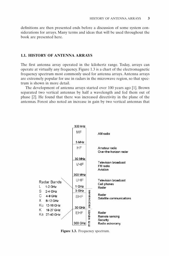
The fi rst antenna array operated in the kilohertz range. Today, arrays can operate at virtually any frequency. Figure 1.3 is a chart of the electromagnetic frequency spectrum most commonly used for antenna arrays. Antenna arrays are extremely popular for use in radars in the microwave region, so that spec-trum is shown in more detail.
The development of antenna arrays started over 100 years ago [1] . Brown separated two vertical antennas by half a wavelength and fed them out of phase [2] . He found that there was increased directivity in the plane of the antennas. Forest also noted an increase in gain by two vertical antennas that
Figure 1.3. Frequency spectrum.
4 ANTENNA ARRAY BASICS
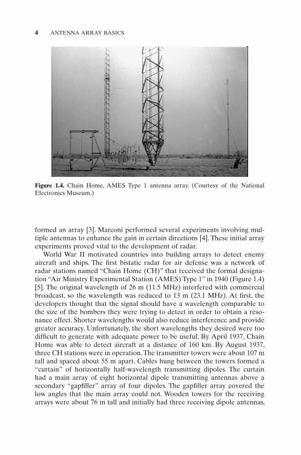
Figure 1.4. Chain Home, AMES Type 1 antenna array. (Courtesy of the National Electronics Museum.)
formed an array [3] . Marconi performed several experiments involving mul-tiple antennas to enhance the gain in certain directions [4] . These initial array experiments proved vital to the development of radar.
World War II motivated countries into building arrays to detect enemy aircraft and ships. The fi rst bistatic radar for air defense was a network of radar stations named “ Chain Home (CH) ” that received the formal designa-tion “ Air Ministry Experimental Station (AMES) Type 1 ” in 1940 (Figure 1.4 ) [5] . The original wavelength of 26 m (11.5 MHz) interfered with commercial broadcast, so the wavelength was reduced to 13 m (23.1 MHz). At fi rst, the developers thought that the signal should have a wavelength comparable to the size of the bombers they were trying to detect in order to obtain a reso-nance effect. Shorter wavelengths would also reduce interference and provide greater accuracy. Unfortunately, the short wavelengths they desired were too diffi cult to generate with adequate power to be useful. By April 1937, Chain Home was able to detect aircraft at a distance of 160 km. By August 1937, three CH stations were in operation. The transmitter towers were about 107 m tall and spaced about 55 m apart. Cables hung between the towers formed a “ curtain ” of horizontally half - wavelength transmitting dipoles. The curtain had a main array of eight horizontal dipole transmitting antennas above a secondary “ gapfi ller ” array of four dipoles. The gapfi ller array covered the low angles that the main array could not. Wooden towers for the receiving arrays were about 76 m tall and initially had three receiving dipole antennas,

HISTORY OF ANTENNA ARRAYS 5
vertically spaced on the tower. As the war progressed, better radars were needed. A new radar called the SCR - 270 (Figure 1.5 ) was available in Hawaii and detected the Japanese formation attacking Pearl Harbor. Unlike Chain Home, it could be mechanically rotated in azimuth 360 degrees in order to steer the beam and operated at a much higher frequency. It had 4 rows of 8 horizontally oriented dipoles and operates at 110 MHz [6] .
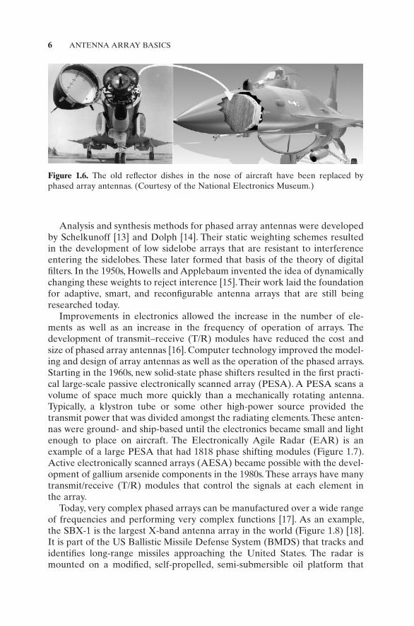
After World War II, the idea of moving the main beam of the array by changing the phase of the signals to the elements in the array (originally tried by F. Braun [7] ) was pursued. Friis presented the theory behind the antenna pattern for a two element array of loop antennas and experimental results that validated his theory [8] . Two elements were also used for fi nding the direction of incidence of an electromagnetic wave [9] . Mutual coupling between ele-ments in an array was recognized to be very important in array design at a very early date [10] . A phased array in which the main beam was steered using adjustable phase shifters was reported in 1937 [11] . The fi rst volume scanning array (azimuth and elevation) was presented by Spradley [12] . The ability to scan without moving is invaluable to military applications that require extremely high speed scans as in an aircraft. As such, the parabolic dish anten-nas that were once common in the nose of aircraft have been replaced by phased array antennas (Figure 1.6 ).
Figure 1.5. SCR - 270 antenna array. (Courtesy of the National Electronics Museum.)
6 ANTENNA ARRAY BASICS
Figure 1.6. The old refl ector dishes in the nose of aircraft have been replaced by phased array antennas. (Courtesy of the National Electronics Museum.)
Analysis and synthesis methods for phased array antennas were developed by Schelkunoff [13] and Dolph [14] . Their static weighting schemes resulted in the development of low sidelobe arrays that are resistant to interference entering the sidelobes. These later formed that basis of the theory of digital fi lters. In the 1950s, Howells and Applebaum invented the idea of dynamically changing these weights to reject interence [15] . Their work laid the foundation for adaptive, smart, and reconfi gurable antenna arrays that are still being researched today.
Improvements in electronics allowed the increase in the number of ele-ments as well as an increase in the frequency of operation of arrays. The development of transmit – receive (T/R) modules have reduced the cost and size of phased array antennas [16] . Computer technology improved the model-ing and design of array antennas as well as the operation of the phased arrays. Starting in the 1960s, new solid - state phase shifters resulted in the fi rst practi-cal large - scale passive electronically scanned array (PESA). A PESA scans a volume of space much more quickly than a mechanically rotating antenna. Typically, a klystron tube or some other high - power source provided the transmit power that was divided amongst the radiating elements. These anten-nas were ground - and ship - based until the electronics became small and light enough to place on aircraft. The Electronically Agile Radar (EAR) is an example of a large PESA that had 1818 phase shifting modules (Figure 1.7 ). Active electronically scanned arrays (AESA) became possible with the devel-opment of gallium arsenide components in the 1980s. These arrays have many transmit/receive (T/R) modules that control the signals at each element in the array.
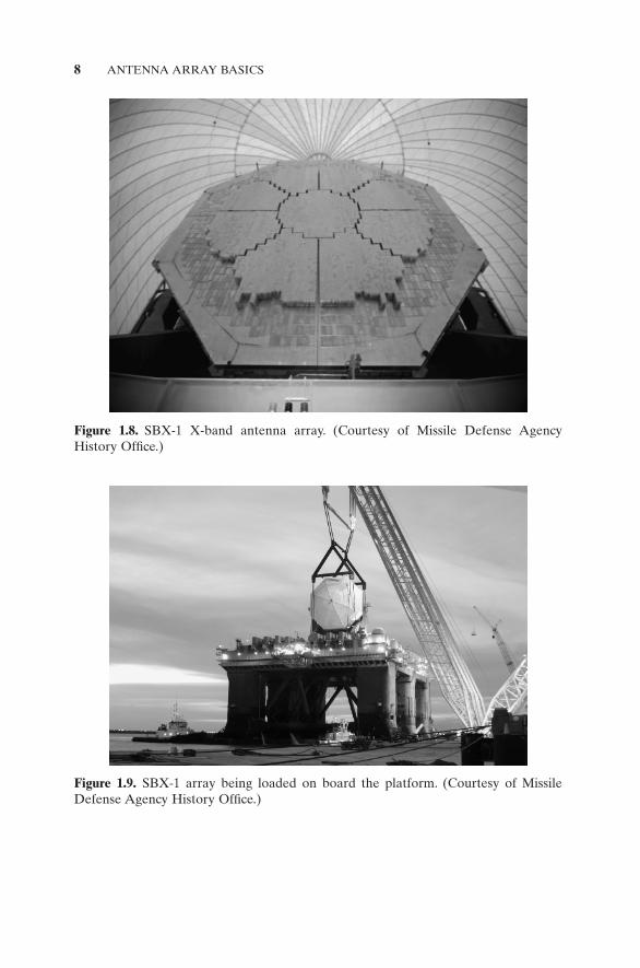
Today, very complex phased arrays can be manufactured over a wide range of frequencies and performing very complex functions [17] . As an example, the SBX - 1 is the largest X - band antenna array in the world (Figure 1.8 ) [18] . It is part of the US Ballistic Missile Defense System (BMDS) that tracks and identifi es long - range missiles approaching the United States. The radar is mounted on a modifi ed, self - propelled, semi - submersible oil platform that

ELECTROMAGNETICS FOR ARRAY ANALYSIS 7
Figure 1.7. EAR array. (Courtesy of the National Electronics Museum.)
travels at knots and is designed to be stable in high winds and rough seas. Through mechanical and electronic scanning, the radar can cover 360 ° in azimuth and almost 90 ° in elevation. There are 45,000 GaAs transmit/receive modules that make up the 284 - m 2 active aperture. Figure 1.9 shows the array being placed on the modifi ed oil platform. A radome is placed over the array to protect it from the elements (Figure 1.10 ).
1.2. ELECTROMAGNETICS FOR ARRAY ANALYSIS
Before delving into the theory of antenna arrays, a review of some basic elec-tromagnetic theory is in order. The frequency of an electromagnetic wave depends on the acceleration of charges in the source. Accelerating charges produce time - varying electromagnetic waves and vice versa. The radiated waves are a function of time and space. Assume that the electromagnetic fi elds are linear and time harmonic (vary sinusoidally with time). The total electro-magnetic fi eld at a point is the superposition of all the time harmonic fi elds at that point. If the fi eld is periodic in time, the temporal part of the wave has a complex Fourier series expansion of the form
E t a en
j nf t
n
( ) ==−∞
∞
∑ 2 0π
(1.1)
where a f E t en
j ntff= ( ) −∫02
0
100 π = Fourier coeffi cients and f 0 is the fundamental
frequency. The fundamental frequency determines where the wave is centered
8 ANTENNA ARRAY BASICS
Figure 1.8. SBX - 1 X - band antenna array. (Courtesy of Missile Defense Agency History Offi ce.)
Figure 1.9. SBX - 1 array being loaded on board the platform. (Courtesy of Missile Defense Agency History Offi ce.)

ELECTROMAGNETICS FOR ARRAY ANALYSIS 9
on the frequency spectrum in Figure 1.3 . If the electromagnetic fi eld is periodic or aperiodic, it has the following temporal Fourier transform pair:
E t E f e dfj ft( ) = ( ) −
−∞
∞
∫ 2π
(1.2)
E f E t e dtj ft( ) = ( )
−∞
∞
∫ 2π
(1.3)
Equations (1.1) , (1.2) and (1.3) illustrate how any time - varying electromag-netic fi eld may be represented by a spectrum of its frequency components. E ( t ) is the superposition of properly weighted fi elds at the appropriate fre-quencies. Superimposing and weighting the fi elds of the individual frequencies comprising the waveform. Traditional electromagnetics analysis examines a single - frequency component, and then it assumes that more complex waves are generated by a weighted superposition of many frequencies.
Equations (1.1) , (1.2) and (1.3) do not take the vector nature of the fi elds into account. A single - frequency electromagnetic fi eld (Fourier component) is represented in rectangular coordinates as
�E t xE ft yE ft zE ftx y y z z( ) = ( ) + +( ) + +( )ˆ cos ˆ cos ˆ cos2 2 2π π ψ π ψ (1.4)
Figure 1.10. SBX - 1 deployed inside a radome. (Courtesy of Missile Defense Agency History Offi ce.)
10 ANTENNA ARRAY BASICS
where x , y , and z are the unit vectors in the x , y , and z directions; E x , E y , and E z are the magnitudes of the electric fi elds in the x , y , and z directions; and ψ y and ψ z are the phases of the y and z components relative to the x compo-nent. Using Euler ’ s identity, (1.4) may also be written as
�E t e j ft( ) = { }Re E 2π
(1.5)
where E represents the complex steady - state phasor (time independent) of the electric fi eld and is written as
E = + +ˆ ˆ ˆxE yE e zE ex yj
zjy zψ ψ
(1.6)
and E x , E y , and E z are functions of x , y , and z and are not a function of t . Maxwell ’ s equations in differential and integral form are shown in Table
1.1 . Note that the e j ω t time factor is omitted, because it is common to all com-ponents. Variables in these equations are defi ned as follows:
E electric fi eld strength (volts/m) D electric fl ux density (coulombs/m 2 ) H magnetic fi eld strength (amperes/m) B magnetic fl ux density (webers/m 2 ) J electric current density (amperes/m 2 ) ρ ev electric charge density (coulombs/m 3 ) J m magnetic current density (volts/m 2 ) ρ mv magnetic charge density (webers/m 3 ) Q e total electric charge contained in S (coulombs) Q m total magnetic charge contained in S (coulombs) S closed surface (m 2 ) C closed contour line (m)
Electric sources are due to charge. Magnetic sources are fi ctional but are often useful in representing fi elds in slots and apertures.
Each of the equations in Table 1.1 is a set of three scalar equations. There are too many unknowns to solve these equations, so additional information is necessary and comes in the form of constitutive parameters that are a function of the material properties. The constitutive relations for a linear, isotropic, homogeneous medium provide the remaining necessary equations to solve for the unknown fi eld quantities.
D E= ε (1.7)
B H= μ (1.8)
J E= σ (1.9)

ELECTROMAGNETICS FOR ARRAY ANALYSIS 11
where the constitutive parameters describe the material properties and are defi ned as follows:
μ permeability (henries/m) ε permittivity or dielectric constant (farads/m) σ conductivity (siemens/m)
Assuming the constant to be scalars is an over simplifi cation. In today ’ s world, antenna designers must take into account materials with special properties, such as
• Composites • Semiconductors • Superconducting materials • Ferroelectrics • Ferromagnetic materials • Ferrites • Smart materials • Chiral materials • Conducting polymers • Ceramics • Electromagnetic bandgap (EBG) materials
Antenna design relies upon a complex repitroire of different materials that will provide the desired performance characteristics.
Spatial differential equations have only general solutions until boundary conditions are specifi ed. If these equations still had the time dependence factor, then initial conditions would also have to be specifi ed. The boundary
TABLE 1.1. Maxwell ’ s Equations in Differential and Integral Form
Law Differential Integral
Faraday ∇ × E = − j ω B − J m
Ampere ∇ × H = j ω D + J
Gauss electric ∇ · D = ρ ev
Gauss magnetic ∇ · B = ρ mv
E l B s J sm⋅ = − ⋅ − ⋅∫ ∫∫ ∫∫d j d dC S S� ω
H l D s J s⋅ = ⋅ + ⋅∫ ∫∫ ∫∫d j d dC S S� ω
D s⋅ =∫∫ d QS
e�
B s⋅ =∫∫ d QS
m�
12 ANTENNA ARRAY BASICS
conditions for the fi eld components at the interface between two media are given by
• The tangential electric fi eld:
n E E Jm× −( ) = −1 2 (1.10)
• The normal magnetic fl ux density:
n B B⋅ −( ) =1 2 ρms (1.11)
• The tangential magnetic fi eld:
n H H Js× −( ) =1 2 (1.12)
• The normal electric fl ux density:
n D D⋅ −( ) =1 2 ρes (1.13)
where subscripts 1 and 2 refer to the two different media, ρ ms is the magnetic surface charge density (coulombs/m 2 ), and ρ es is the electric surface charge density (webers/m 2 ).
Maxwell ’ s equations in conjunction with the constitutive parameters and boundary conditions allow us to fi nd quantitative values of the fi eld quantities.
Power is an important antenna quantity and has units of watts or volts times amps. Multiplying the electric fi eld and the magnetic fi eld produces units of W/m 2 or power density. The complex Poynting vector describes the power fl ow of the fi elds via
S E H= ×{ }1
2Re *
(1.14)
Note that the direction of propagation (direction that S points) is perpendicu-lar to the plane containing the E and H vectors. S is the power fl ux density, so ∇ · S is the volume power density leaving a point. A conservation of energy equation can be derived in the form of
E H ds E J
E H× ⋅ = − ⋅ − +⎛⎝⎜
⎞⎠⎟∫∫ ∫∫∫ ∫∫∫* *dv j dvω ε μ2 2
2 2 (1.15)
The terms 122ε E and 12
2μ H are the electric and magnetic energy densities, respectively. Finally, E · J * represents the power density dissipated.
SOLVING FOR ELECTROMAGNETIC FIELDS 13
1.3. SOLVING FOR ELECTROMAGNETIC FIELDS
The sources that generated the current on the antenna or the voltage across the terminal of the antenna must be known in order to calculate the fi elds radiated by the antenna. There is an analytical approach to fi nding fi elds for some very simple antennas in which the current on the antenna is postulated. In most practical cases, however, the fi elds must be found using numerical methods. This section presents an approach for analytically fi nding fi elds for simple antennas that also forms the basis for some numerical approaches in the frequency domain.
1.3.1. The Wave Equation
A time - varying current on an antenna is the input to a linear system called free space. The output is the radiated electromagnetic fi eld. The simplest conceivable antenna is called an isotropic point source, and it radiates equally in all directions. At a constant distance from the source (the surface of an imaginary sphere), the amplitude and phase of the electromagnetic fi eld radiated by the point source is the same at a given instant in time. Point sources don ’ t really exist. However, certain radiating objects, such as stars, behave as though they were point sources when the observer is far away. If a point source is modeled as a spatial impulse, then an impulse response must exist for free space. Once the impulse response is known, then the output is found by convolving an input with the impulse response. This approach to fi nding the fi elds radiated by an antenna is identical to fi nding the impulse response of a fi lter.
The quest for the impulse response of free space (also called the free - space Green function) begins with the vector wave equation for the electric fi eld with only electric sources. It is derived by taking the curl of Faraday ’ s law and substituting Ampere ’ s law into the right - hand side.
∇ × ∇ × = − ∇ × = − +( ) = −E H E J E Jj j j k jωμ ωμ ωε ωμ2
(1.16)
The left - hand side of this equation may be converted to a more convenient form using the vector identity ∇ × ∇ × E = ∇ ( ∇ · E ) − ∇ 2 E and substituting Gauss ’ law.
∇ + = + ∇2 2 1
E E Jk j evωμσε
ρ
(1.17)
This equation is very useful when there are no sources, because E is easy to fi nd. Unfortunately, the sources are in terms of both J and ρ ev . Thus, in order to calculate the fi elds radiated by an antenna or scattering object, both J and ρ ev must be known.

14 ANTENNA ARRAY BASICS
Our goal is to have one vector quantity on the left - hand side of the equa-tion and one source quantity on the right - hand side. In order to achieve this goal, a wave equation is found for the magnetic vector potential A . Then, E and H are found from A . The derivation of the wave equation for the vector magnetic potential starts by defi ning A from Gauss ’ law, ∇ · B = 0, and the vector identity ∇ · ∇ × A = 0.
B A= ∇ × (1.18)
Substituting (1.18) into Faraday ’ s law gives
∇ × +( ) =E Ajω 0 (1.19)
Recognizing that (1.19) fi ts the form of the vector identity ∇ × ∇ V = 0, E is defi ned as
−∇ = +V jE Aω (1.20)
or
E A= − − ∇j Vω (1.21)
where V is an arbitrary scalar potential. The next step is to substitute (1.18) and (1.21) into Ampere ’ s law to get
1μ
ωε ω∇ × ∇ × = − − ∇( ) +A A Jj j V
(1.22)
which may be rewritten as
∇ + = − + ∇ ∇⋅ +( )2 2A A J Ak j Vμ ωμε (1.23)
by using the vector identity ∇ × ∇ × A = ∇ ( ∇ · A ) − ∇ 2 A , defi ning k 2 = ω 2 μ ε , and rearranging the terms. Since V and A are arbitrary (we took them from some vector identities), we can defi ne our own relationship between them. Looking at (1.23), the choice for relating V and A that would greatly simplify the equation is
∇⋅ + =A j Vωεμ 0 (1.24)
This relationship between A and V is known as the Lorentz condition. Using the Lorenz condition in (1.23) yields the wave equation.
∇ + = −2 2A A Jk μ (1.25)
SOLVING FOR ELECTROMAGNETIC FIELDS 15
A similar derivation for magnetic sources yields another wave equation.
∇ + = −2 2F F Jmk ε (1.26)
where F is the electric vector potential for the fi ctional magnetic current.
1.3.2. Point Sources
If the source in (1.25) is an impulse function or a point source, then it is rep-resented in rectangular coordinates as
J x y z J r x y z′ ′ ′( ) = ′( ) = ′( ) ′( ) ′( ), , δ δ δ (1.27)
The fi eld characteristics of a point source are most simply defi ned in terms of θ and φ . The z - component of (1.25) outside the origin.becomes
10
22 2
r rr
Ar
k Azz
∂∂
∂∂
+ =
(1.28)
The θ and φ variations are zero, so the wave equation is only a function of r , the distance from the origin to the point of observation. The impulse response of free space, G ( r ), is found by substituting A z = G ( r )/ r into (1.28) to get
d rdr
k r2
22 0
GG
( ) + ( ) =
(1.29)
where r = r r = x x + y y + z z and r = | r |. Solving this equation for G ( r ) results in two solutions. Since the assumed time dependence is e j ω t , the fi rst solution represents waves traveling away from the point source (transmit antenna)
G r
er
jkr
( ) =−
4π
(1.30)
and the second solution represents waves traveling toward the point source (receive antenna)
G r
er
jkr
( ) =4π
(1.31)
Theoretically, real antennas consist of a collection of point sources. Their far - fi eld patterns are a convolution of the current on the antenna ( J ) with G . An antenna may be thought to consist of point sources distributed throughout space. When a point source is at ( x ′ , y ′ , z ′ ) instead of at the origin, it is repre-sented as

16 ANTENNA ARRAY BASICS
J R x x y y z z
rr r
( ) = − ′( ) − ′( ) − ′( )
=′
− ′( ) − ′( ) − ′( )
δ δ δ
πδ δ θ θ δ φ φ1
4 2
(1.32)
If the point source is at the origin, then
J r
rr′( ) =
′′( )1
4 2πδ
(1.33)
and the free - space Green function is
G r r
eR
jkR
′( ) =−
4π (1.34)
where r ′ = x ′ x + y ′ y + z ′ z , r ′ = | r ′ |, and R = | r − r ′ |. To summarize, the electromagnetic fi elds radiated by an antenna may be
found by the following steps:
1. Postulate the current on the antenna ( J ). This may be done experimen-tally, analytically, numerically, or a reasonable guess.
2. Calculate A by convolving the J and or F by convolving the J m with G for each vector component:
A J= ′( ) ′
−
′∫∫∫μ
πr
eR
dvjkR
v 4 (1.35)
F Jm= ′( ) ′
−
′∫∫∫ε
πr
eR
dvjkR
v 4 (1.36)
3. Calculate H :
H A F F= ∇ × − − ∇ ∇( )1 1
μω
ωμεj j i
(1.37)
4. Calculate E from Ampere ’ s law:
E H F= ∇ × − ∇ ×1 1
jωε ε (1.38)
The next two subsections demonstrate this procedure on simple antennas.

SOLVING FOR ELECTROMAGNETIC FIELDS 17
1.3.3. Hertzian Dipole
A Hertzian dipole is a straight - wire antenna that is 2a long and is very small compared to a wavelength (2 a << λ ). We follow the steps of the previous section to fi nd the radiated fi elds. If the antenna lies along the z axis, then it can be modeled as a line of point sources from z = − a to z = a (Figure 1.11 ). Since the antenna is so small, the current is approximately a constant, J = z I 0 δ ( x ′ ) δ ( y ′ ) along the length of the wire. The magnetic vector potential is given by
A I x y
er z
dx dy dzz a
ajk r z
= ′( ) ′( )− ′
′ ′ ′− −∞
∞
−∞
∞− − ′
∫ ∫ ∫μ δ δπ0
4 (1.39)
This integral simplifi es to
A
a I er
z
jkr
= ( ) −μπ
24
0
(1.40)
given the following assumptions:
R r z r= − ′ �
2a� λ
2a R�
I z I′( ) =is a constant 0
This solution has a variable r that is one of the dimensions of a spherical coordinate system yet has a vector component that is in a rectangular
Figure 1.11. Hertzian dipole along the z axis.

18 ANTENNA ARRAY BASICS
coordinate system. In order to put everything in one coordinate system, the z component is converted to spherical coordinates.
A r= −( )−2
40a I
re jkrμ
πθ θˆ cos ˆ sinq
(1.41)
The electric and magnetic fi elds are derived from (1.35) and (1.36):
E r= +⎛
⎝⎞⎠ − − − +⎛
⎝⎜⎞⎠⎟
⎡⎣
24
21 10
2 3
2
2 3
a I Zk
jkr r
kr
jkr r
μπ
θ θcos sinˆ q⎢⎢⎤⎦⎥
−e jkr
(1.42)
H = +⎛
⎝⎞⎠
−24
102
a I jkr r
e jkrμ θπsin j
(1.43)
where Z is the impedance given by
Z = μ
ε (1.44)
A short distance from the antenna, the 1/ r 2 and 1/ r 3 terms quickly become negligible compared to the 1/ r term:
E =
−
j aZI ke
r
jkr
24
0 sinθπ
q
(1.45)
H =
−
j aZI ke
r
jkr
24
0 sinθπ
j
(1.46)
Equations (1.45) and (1.46) are far - fi eld equations because the electric and magnetic fi elds are orthogonal to each other and to the direction of propaga-tion. Another property of the far fi eld evident from these equations is that the electric and magnetic fi elds are related by
E r H= − ×Zˆ (1.47)
H r E= ×1
Zˆ
(1.48)
The power fl ow is shown to be in the radial direction by calculating the complex Poynting vector given by
12 8
02
02 2 2
2 2E H r× =* ˆ sinI Z a k
rθ
π (1.49)
Thus, the power radiated is a function of 1/ r 2 , which is the same as an indi-vidual point source. Unlike the isotropic point source, the Hertzian dipole has

SOLVING FOR ELECTROMAGNETIC FIELDS 19
preferred directions of radiation and reception as given by the sin θ term. It is also polarized: The electric fi eld is described by a vector.
1.3.4. Small Loop
Point sources may also be placed side - by - side to form a loop as shown in Figure 1.12 . Assume the loop is so small that the current is constant on the loop and is given by
I
r ar
aφ δ θ δ φ λ( ) = − °( ) −( )90 ˆ, �
(1.50)
The magnetic vector potential is found from
A = ′( )
′ ′ ′ ′ ′∞
−∫∫∫ ˆ sinj000
22
4
ππ μ φπ
θ θ φIR
e r dr d djkR
(1.51)
where R is given by
R r r r r r r r r r r
r a ar
= − ′ = − ′( )⋅ − ′( ) = + ′ − ⋅ ′
= + − ′ −
2 2
2 2
2
2 sin cos cos sθ φ φ iin sinφ φ′( ){ } (1.52)
The observation distance is assumed to be much greater than the loop diam-eter ( r >> a ). Factor r out of the radical, then the a 2 / r 2 inside the radical is very small and can be ignored. Since a / r is also very small, the binomial expansion for the square root gives an accurate approximation:
Rr
y
z
x
a
Figure 1.12. Small loop model.

20 ANTENNA ARRAY BASICS
R r a� − ′ + ′( )sin cos sin sinθ φ φ φ (1.53)
The second term contributes little to the amplitude of the magnetic vector potential, because its maximum value is a . For instance, if r is 100 m and a is 1 m, then the amplitude of A decreases by about 1%. Thus, R � r in the denominator. However, the same 1% increase in R produces a 180 ° phase shift at a frequency of 600 MHz, and (1.53) must be used in the phase term. Making the proper substitutions into (1.51) yields
A = ′ − °( ) ′ −( ) − − ′+ ′( )[ ]μ
πδ θ δ θ φ φ φ φI r a e
r
jk r a0
490 sin cos cos sin sin
′′ ′ ′ ′ ′∫∫∫∞
r dr d d2
0
2
00
sinθ θ φππ
j
(1.54)
Integrating over θ ′ and r ′ , substituting the rectangular representation of φ ′ , and making the small phase angle approximation e jx � 1 + jx reduces the equation to
A = − ′ + ′( ) + ′ +
−μπ
φ φ θ φ φ φβI ae
rx y jka
j r0
41ˆ sin ˆ cos sin cos cos sin sin ′′( )[ ] ′∫ φ φ
π
d j0
2
(1.55)
After performing the fi nal integration and substituting ˆ ˆ sin ˆ cosj = − +x yφ φ ,
then
A =
−j k a I er
jkrμ π θπ
20
4sin j
(1.56)
The magnetic fi eld is
H A= ∇ × = − ∂
∂( ) = − −1 1
4
2
μ μθ
πφr r
rAMk
re jkrˆ sin ˆq q
(1.57)
where M = π a 2 I 0 is the dipole moment of the small current loop. The electric fi eld is given by
E r H= − × = − −Z
MZkr
e jkrˆ sin ˆ2
4θ
πq
(1.58)
These equations have a form similar to those for the Hertzian dipole and are called dual formulations. The analysis of larger loops is more complicated because one cannot assume that a is small compared to λ , so the current is not constant in amplitude and phase around the loop.

SOLVING FOR ELECTROMAGNETIC FIELDS 21
1.3.5. Plane Waves
A plane wave is a transverse electromagnetic (TEM) wave having constant amplitude and phase in an infi nite plane in space at an instant in time. A TEM wave has the electric and magnetic fi elds orthogonal to the direction of propa-gation. The plane wave travels in the direction orthogonal to the plane. Thus, a plane wave is described by a vector or an angle of propagation and magni-tude and phase of the fi eld in the plane. The propagation vector points in the direction of propagation and is written as
k = + +k x k y k zx y zˆ ˆ ˆ (1.59)
where the propagation constants in the x , y , and z directions are given by
k kx
x
= =2πλ
θ φsin cos
k ky
y
= =2πλ
θ φsin sin
k kz
z
= =2πλ
θcos
and the projections of the wavelength onto the x , y , and z directions are given by λ x , λ y , and λ z .
Even though the point source and plane wave are mathematical and con-ceptual models, we relate them in a very practical way, because we are often only interested in a portion of the angular extent of the fi eld. When the spheri-cal wave of a transmit antenna impinges on the receive antenna, how spherical does it look? As the distance between the antennas increases, the incident wave looks less curved. At some distance R the incident wave can be said to be a plane wave relative to the receive antenna or over a local extent. This approximation is extremely important in antenna measurements. As a rule of thumb (and IEEE defi nition [19] ), a receive antenna is in the far fi eld of a point source when the maximum phase deviation across the aperture is less than λ /16 or π /8 radians. Figure 1.13 shows the simple trigonometric derivation for the far - fi eld formula given by
R
D= 2 2
λ (1.60)
where R is the distance from the point source to the receive antenna and D is the largest dimension of the receive antenna. For high - performance (low - sidelobe) antennas, a stricter error tolerance may be needed, and the far fi eld will be a greater distance from the antenna.

22 ANTENNA ARRAY BASICS
Figure 1.13. Derivation of the defi nition of far fi eld.
1.4. ANTENNA MODELS
Antennas transmit and/or receive signals. From a circuit point of view, the antenna appears as a load on a transmission line. An antenna is matched when the signal from the transmission line is radiated and not refl ected back to the transmitter. Determining the impedance of this load and matching it to the feed line is important. An antenna may also be considered a fi lter. The fi lter passes electromagnetic waves with desirable frequency, directional, and polar-ization attributes. These models are widely used in antenna design and are described in the next sections.
1.4.1. An Antenna as a Circuit Element
A radiating system consists of an oscillating source to generate a signal, a transmission line or waveguide, and an antenna to transform that signal to an electromagnetic wave. Not all the power generated by the transmitter goes to the antenna. Transmission lines and connectors between the source and antenna become potential sources for degradation due to mismatches, radia-tion loss, and heat loss. A guided wave traveling along a transmission line refl ects from any discontinuity, or point in the transmission path where the impedance changes. These refl ections set up a standing wave in the line which
ANTENNA MODELS 23
stores energy and reduces the amount of power delivered to the intended load (antenna). The standing wave ratio (SWR) is the ratio of the maximum to minimum value of the voltage standing wave established by the refl ections. SWR is a common measure used in matching guided wave components and is calculated by
SWR = = +
−VV
L
L
max
min
11
ΓΓ
(1.61)
where Γ L is the refl ection coeffi cient at the discontinuity. An SWR of 1 indi-cates a perfect match. The refl ection coeffi cient is the ratio of the refl ected to incident voltages at the discontinuity
ΓL
L
L
VV
Z ZZ Z
= = −+
reflected
incident
0
0 (1.62)
where Z 0 is the transmission line impedance and Z L is the discontinuity imped-ance. Frequently, Γ L is also called s 11 from the s parameters. Impedances are a function of frequency, so SWR is often used to establish the frequency range or bandwidth in which an antenna can be used. In most cases, an SWR < 2 or s 11 < − 10 dB defi ne the bandwidth limits. One needs to be careful comparing the bandwidth of two antennas. Sometimes, for receive antennas, the band-width is defi ned over the frequency range when VSWR ≤ 3. It is more impor-tant to have a low VSWR for a transmit antenna, because the refl ected power can be high enough to damage circuits.
Signal power escapes from the circuit through radiation or heating. Radiation losses occur when the signal leaks from the transmission path by way of connectors or the open sides of microstrip lines. Thermal losses result when resistance in the transmission line converts part of the signal to heat. Resistance comes from the imperfect conductors and dielectrics that make up the transmission line. The reduced power delivered to the antenna terminals is given by
P Pt h r L= −( )δ δ 1 2Γ TR
(1.63)
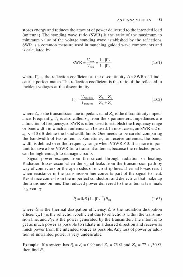
where δ h is the thermal dissipation effi ciency, δ r is the radiation dissipation effi ciency, Γ L is the refl ection coeffi cient due to refl ections within the transmis-sion line, and P TR is the power generated by the transmitter. The intent is to get as much power as possible to radiate in a desired direction and receive as much power from the intended source as possible. Any loss of power or addi-tion of unwanted power is very undesirable.
Example. If a system has δ h = δ r = 0.99 and Z 0 = 75 Ω and Z L = 77 + j 30 Ω , then fi nd P t .

24 ANTENNA ARRAY BASICS
ΓL
jj
jj
= + −+ +
= ++
77 30 7577 30 75
2 30152 30
The resulting transmitted power is
P Wt = −( ) ⇒ =. . % . %99 1 19 10 94 32 2 transmitted
1.4.2. An Antenna as a Spatial Filter
Antennas do not radiate power isotropically (equally in all directions). Instead, an antenna is a spatial fi lter which concentrates power in certain directions at the expense of decreasing the power radiated in other directions. The power density (W/m 2 ) radiated by an antenna is given by
S
rE Er = +( )1
2 22 2
η θ φ
(1.64)
Directivity compares the power density in a designated direction to the average power density. Unless otherwise specifi ed, directivity implies that the maximum value of directivity is given by
DS
S d dr
r
=∫∫
4
00
2
πθ θ φππ
max
sin
(1.65)
The gain of the antenna is the ratio of the power radiated in a particular direction to power delivered to the antenna. Gain differs from directivity because gain includes losses.
Directivity is always greater than or equal to gain. The denominator in (1.65) can be replaced by power delivered to the antenna, thus avoiding the double integration. Gain and directivity are related through the radiation effi ciency, δ e , the ratio of the power radiated by the antenna to the power input to the antenna
G Deθ φ δ θ φ, ,( ) = ( ) (1.66)
The realized gain includes the losses due to the mismatch of the antenna input impedance to a specifi ed impedance. Realized gain is frequently used by engi-neers when integrating the antenna into the system. When gain is written without any angular dependence, G , it implies the maximum gain of the antenna. Since G is a power ratio, it is often expressed in decibels
G G GdB = =10 1010log log (1.67)
Figure 1.14 shows a three - dimensional plot in cylindrical coordinates of a relative antenna radiation pattern far from the antenna as a function of θ and

ANTENNA MODELS 25
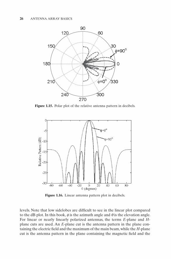
φ , where θ is measured in the radial direction, φ is in the horizontal plane, and the pattern amplitude in the vertical direction. Relative means that no abso-lute units of power are associated with the pattern, but the power between two different angles are of the correct ratio. A relative antenna pattern means that the maximum value is normalized to 1 or 0 dB. The direction of maximum gain is at the center of a large lobe called the main beam, while smaller lobes are called sidelobes, and the zero - crossings are called nulls. Bigger lobes in some directions indicate greater gain in those directions.
Three - dimensional antenna patterns (Figure 1.14 ) provide an overall quali-tative evaluation of the antenna ’ s spatial response. Accurately determining sidelobe levels, null locations, and beamwidth require the use of two - dimensional cuts, however. An antenna pattern cut is the two - dimensional antenna pattern measured on a great circle around the antenna. Figure 1.15 shows two orthogonal polar magnitude plots of the three - dimensional pattern in Figure 1.14 ( φ = 0 ° and φ = 90 ° ). These same patterns appear as rectangular plots in Figure 1.16 (dB) and in Figure 1.17 (linear). The polar plot is useful for appreciating the angular layout of the pattern. The rectangular plots are used to precisely locate nulls, determine beamwidth, and establish sidelobe
f
Figure 1.14. Three - dimensional antenna pattern.
26 ANTENNA ARRAY BASICS
Figure 1.15. Polar plot of the relative antenna pattern in decibels.
Figure 1.16. Linear antenna pattern plot in decibels.
levels. Note that low sidelobes are diffi cult to see in the linear plot compared to the dB plot. In this book, φ is the azimuth angle and θ is the elevation angle. For linear or nearly linearly polarized antennas, the terms E - plane and H - plane cuts are used. An E - plane cut is the antenna pattern in the plane con-taining the electric fi eld and the maximum of the main beam, while the H - plane cut is the antenna pattern in the plane containing the magnetic fi eld and the

ANTENNA MODELS 27
maximum of the main beam. Antenna patterns are often normalized to the peak of the main beam.
The beamwidth of an antenna may mean either (a) the angular separation between the half - power (3 dB) points on either side of the peak of the main beam (most common engineering defi nition) or (b) the angular separation between the fi rst nulls on either side of the main beam (defi nition often used in optics and physics). If the antenna pattern is not symmetrical, then the beamwidth must be specifi ed in the plane of the antenna pattern cut. Usually the beamwidth is specifi ed in two orthogonal antenna pattern cuts.
Another important antenna gain characteristic is effective (or equivalent) isotropically radiated power (EIRP). EIRP is the gain of the transmitting antenna multiplied by the power delivered to its input.
EIRP = PGt (1.68)
It is the transmitter – antenna combination that determines the transmitted power of a system. EIRP is especially important for satellite antennas where power and antenna size are at a premium.
1.4.3. An Antenna as a Frequency Filter
Antennas transmit and receive certain frequencies better than other frequen-cies, making the antenna a frequency fi lter. Antennas that respond to a very small range of frequencies are known as narrowband or resonant antennas, and those that respond over a wide range of frequencies are known as broad-band antennas. Usually, a narrowband antenna is quite simple in shape, like
Figure 1.17. Linear rectangular antenna pattern.

28 ANTENNA ARRAY BASICS
a dipole. The simplicity allows the current to resonate over a well - defi ned region. On the other hand, broadband antennas have a more complex shape, like a helix or spiral. The complex shape gives the antenna the ability to reso-nate at many different adjacent frequencies.
The bandwidth is usually stated in one of three ways:
• Percent of center frequency
BW hi lo
center
= − ×f ff
100
(1.69)
• Ratio of high and low frequencies
BW hi
lo
= ff
(1.70)
• Range of frequencies
BW hi lo= −f f (1.71)
Broadband implies that the antenna has a 10% or higher bandwidth, or it operates over at least an octave ( f hi / f lo = 2). The term ultra - wide band (UWB) refers to antennas that have very broad bandwidths [20] . The Defense Advanced Research Projects Agency (DARPA) defi nes UWB as BW ≥ 25% and the Federal Communications Commission (FCC) defi nes UWB as BW ≥ 20%.
Defi ning the values of f hi and f lo are not easy. Some ways this is done include:
• A function of antenna gain. f center is the frequency of the highest antenna gain, f hi is the highest frequency at which the gain has not fallen below − 3 dB, and f lo is the lowest frequency at which the gain has not fallen below − 3 dB.
• A function of SWR. f center is the frequency at which the antenna is best matched, f hi is the highest frequency at which the SWR is still less than 2, and f lo is the lowest frequency at which the SWR is still less than 2. An equivalent defi nition is the refl ection coeffi cient ( s 11 ) is less than 1/3 or − 10 dB. Sometimes receive antennas may be specifi ed using a VSWR > 2.
• A function of some important antenna performance feature. f hi and f lo defi ne the bandwidth over which the performance indicator lies within acceptable bounds.
The bandwidth can refer to either the instantaneous bandwidth or opera-tional bandwidth. Instantaneous bandwith is the bandwidth of the signal at

ANTENNA MODELS 29
the antenna. The operational bandwidth is the bandwidth of the antenna and is greater than the instantaneous bandwidth.
Example. Is an antenna that has a bandwidth over the AM broadcast fre-quencies a broadband antenna? f hi = 1600 kHz and f lo = 540 kHz ⇒ f center = 1070 kHz BW = f hi − f lo = 1060 kHz, BW = f hi − f lo / f center × 100 = 1060/1070 × 100 = 99.065%, and BW = f hi / f lo = 1600/540 = 2.963. This antenna would be broadband.
1.4.4. An Antenna as a Collector
As mentioned previously, an antenna collects electromagnetic waves in a similar manner that a bucket collects rain. A time - varying electromagnetic fi eld incident on an antenna causes charges in the receiving antenna to oscil-late. If the charges oscillate at the same rate as the incident fi eld, some of the electromagnetic wave re - radiates as a wave at the same frequency as the inci-dent wave. The remainder of the wave converts into heat or is delivered to a load such as a radio receiver. The amount of current induced by an incident wave may be represented by a current density distributed over an area called the collecting aperture ( A c ). The areas over which the collected energy is coupled to a receiver, scattered, and dissipated are represented respectively by the effect aperture ( A e ), the scattering aperture ( A s ), and the loss aperture ( A L ) [21] .
A A A Ac e s L= + + (1.72)
All the aperture terms have units of area, but they are not necessarily related to the projected area of the antenna. The effective aperture represents that part of the incident power density delivered to the receiving system, while the scattering and loss apertures represent those parts of the incident power density that are scattered and dissipated as heat.
The power delivered to the output of a receiving antenna is the same as the incident power density multiplied by the effective aperture.
P S Ar i e= (1.73)
Equation (1.73) is very similar to EIRP, as we would expect from a reciprocal device. The effective aperture is related to gain by
G
Ae= 42
πλ
(1.74)
Effective aperture is a term reserved for receive antennas, whereas gain describes both transmitting and receiving antennas.

30 ANTENNA ARRAY BASICS
Example. Find the gain of a 50 - m - diameter radio telescope parabolic refl ector antenna at 1 GHz. Assume that A c = A e = area of the refl ector aperture.
Ae = π252
Then
G =× ×( )
=4 25
3 10 1 1054 4
2 2
8 9 2
π. dB
1.4.5. An Antenna as a Polarization Filter
Polarization of an electromagnetic wave describes how the magnitude and orientation of the electric fi eld vector changes as a function of time at a given point in space. The polarization of an antenna is defi ned as the polarization of the wave transmitted by the antenna. The orientation of the time - varying electric fi eld is important because it determines the orientation of the current induced in an object. Remember that the current fl ows in the same direction as the electric fi eld. Thus, a time - varying electric fi eld with z - directed polariza-tion will produce a time - varying current in a wire parallel to the fi eld, no current in a wire perpendicular to the z direction, and some time - varying current in a wire oriented between parallel and perpendicular. The orientation of a transmitting antenna, receiving antenna, and any scatterer in between affects the amount of power received.
If we assume that the electric fi eld vector is a plane wave traveling in the z direction, the electric fi eld lies in the x – y plane. The time harmonic repre-sentation of a single frequency electric fi eld is
�E t E t kz E t kzx y y( ) = −( ) + − +( )0 0cos cosω ωˆ ˆx yΨ (1.75)
We may examine the vector at a point in space ( z = 0):
E x y= +E Ex yˆ ˆ (1.76)
Equating (1.75) to (1.76) results in these defi nitions:
E E tx x= ( )0 cos ω (1.77)
E E ty y y= +( )0 cos ω Ψ (1.78)
Solving for cos( ω t) produces
cos ωt
EE
x
x
( ) =0
(1.79)

ANTENNA MODELS 31
Using trigonometry, (1.79) can be written as
sin ωt
EE
x
x
( ) = − ⎛⎝⎜
⎞⎠⎟1
0
2
(1.80)
With a little manipulation, the following equation describes the orthogonal components of the propagating plane wave:
aE bE E cEx x y y2 2 1− + = (1.81)
where
a
Eb
E Ec
Ex y
y
x y y y y
= = =1 2 1
02 2
0 02
02 2cos
,sin
cos,
cosΨΨ
Ψ Ψ (1.82)
This equation for an ellipse tells us that at any point in space, the tip of the electric fi eld vector traces an ellipse over a period of time. Conversely, if a wave is frozen in time, the tip of the E vector along the propagation path traces out the same ellipse. For this reason, we say that the wave is elliptically polarized.
The electric fi eld vector rotates either clockwise or counterclockwise. If you place your right thumb in the direction of wave propagation, and your fi ngers curve in the direction of the E fi eld trajectory, the wave is said to be right - hand polarized (RHP). On the other hand (literally), if the trajectory is such that the thumb of the left hand can be pointed in the direction of wave propaga-tion, and the fi ngers curve in the direction of the E fi eld trajectory, the wave is left - hand polarized (LHP). The relative phase determines the handedness of the wave. For 0 ° < Ψ y < 180 ° the wave is LHP, and for 180 ° < Ψ y < 360 ° the wave is RHP. Figure 1.18 shows the electric fi eld rotation for left - hand and right - hand elliptical polarization.
Figure 1.18. Rotation of the electric fi eld for right - hand and left - hand polarization.
32 ANTENNA ARRAY BASICS
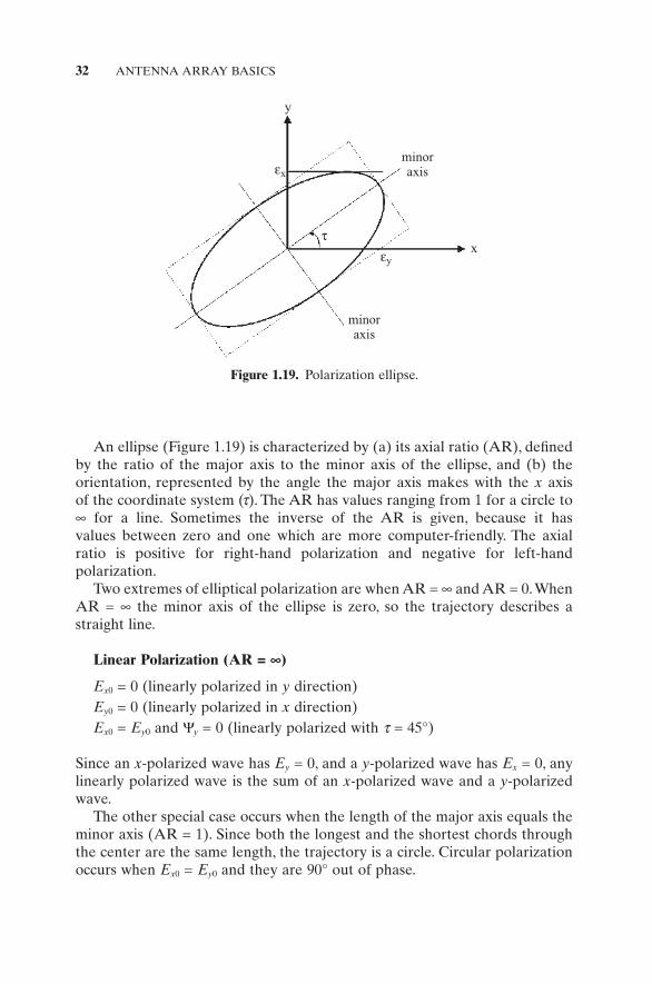
An ellipse (Figure 1.19 ) is characterized by (a) its axial ratio (AR), defi ned by the ratio of the major axis to the minor axis of the ellipse, and (b) the orientation, represented by the angle the major axis makes with the x axis of the coordinate system ( τ ). The AR has values ranging from 1 for a circle to ∞ for a line. Sometimes the inverse of the AR is given, because it has values between zero and one which are more computer - friendly. The axial ratio is positive for right - hand polarization and negative for left - hand polarization.
Two extremes of elliptical polarization are when AR = ∞ and AR = 0. When AR = ∞ the minor axis of the ellipse is zero, so the trajectory describes a straight line.
Linear Polarization (AR = ∞ )
E x 0 = 0 (linearly polarized in y direction) E y 0 = 0 (linearly polarized in x direction) E x 0 = E y 0 and Ψ y = 0 (linearly polarized with τ = 45 ° )
Since an x - polarized wave has E y = 0, and a y - polarized wave has E x = 0, any linearly polarized wave is the sum of an x - polarized wave and a y - polarized wave.
The other special case occurs when the length of the major axis equals the minor axis (AR = 1). Since both the longest and the shortest chords through the center are the same length, the trajectory is a circle. Circular polarization occurs when E x 0 = E y 0 and they are 90 ° out of phase.
minoraxis
minoraxis
y
xey
ex
t
Figure 1.19. Polarization ellipse.

ANTENNA MODELS 33
Circular Polarization (AR = 1)
E x 0 = E y 0 , Ψ y = +90 ° (left - circularly polarized) E x 0 = E y 0 , Ψ y = − 90 ° (right - circularly polarized)
If the receive antenna is not polarization - matched to the incoming electro-magnetic wave, then it will not receive the maximum possible power. The receive polarization of an antenna is defi ned as the polarization of an incident wave that results in maximum power at the antenna terminals. It is related to the (transmit) polarization of the antenna in the same plane of polarization by having the same
1. Axial ratio 2. Sense of polarization 3. Spatial orientation
The power received by an antenna is multiplied by a polarization effi ciency or polarization mismatch factor to account for the polarization mismatch between an incident wave and an antenna ’ s receive polarization. This polariza-tion effi ciency is calculated by taking the inner product of the incident wave polarization vector and the complex conjugate of the receive antenna polariza-tion vector.
p e ei r= ⋅ ∗ˆ ˆ (1.83)
where
ei = =polarization vector of incident wave incident
incident
EE
(1.84)
er = =polarization vector of receive antenna antenna
antenna
EE
(1.85)
The received power is given by
P pA Sr e= (1.86)
If the receive antenna has the same polarization as the transmit antenna, then there is a perfect match.
Example. Given the following values of E x , E y , and Ψ y , what is the polariza-tion of the fi eld?
34 ANTENNA ARRAY BASICS
E x E y Ψ y Answer
1 0 45 ° x linear 0.707 0.707 0 ° linear 45 ° from x axis 0.707 0.707 90 ° LHP circular 0.867 0.5 180 ° linear 60 ° from x axis 0.867 0.5 90 ° elliptical
1.5. ANTENNA ARRAY APPLICATIONS
Antenna arrays fi nd applications over a wide range of frequencies. Some common types of systems that depend on arrays are described in this section.
1.5.1. Communications System
A communications system sends information from one point to another. For the receiver to detect the signal, the signal must be strong enough to be dis-tinguished from noise. Radio receivers are typically rated by the minimum detectable ratio of received power to noise power, also known as the signal - to - noise ratio (SNR).
Average power density at a distance R from an isotropic radiator is the total radiated power divided by the surface area of a sphere, P t /4 π R 2 . Increasing R to 2R reduces the average power density on the new imaginary sphere by one forth. The transmitter power density incident on an object, therefore, depends on the transmitted power, the antenna gain (which depends upon the antenna effi ciency and the directivity function of azimuth and elevation), and the range from the radiator to the target:
S
PGR
it t=
4 2π (1.87)
In reality, electromagnetic waves encounter such problems as atmospheric absorption, particulate scattering, and obstacle scattering. To account for these additional losses, a loss factor ( L < 1.0) is included in the calculation of power density.
S
PG LR
it t=
4 2π (1.88)
The power density incident on the receiving antenna is multiplied by the effec-tive aperture to get the power delivered to the output terminals of the antenna. The resulting equation is known as the Friis transmission formula (Figure 1.20 ) [22] .

ANTENNA ARRAY APPLICATIONS 35
P
PG LAR
rt t e=4 2π
(1.89)
Example. A cellular phone transmits 1 W of power at 840 MHz. Assume the phone is always between 100 m and 3 km of a base station. What is the minimum sensitivity of the receiver at the base station? The antennas are monopoles with gains of 1.5.
P
PG G L
Rr
t t r=( )
= × × × ××( )
λπ π
2
41 1 5 1 5 1 0 357
4 30002
2
2
. . .
1.5.2. Radar System
A radar system determines the characteristics of a target by radiating electro-magnetic waves toward a target and analyzing the waves re - radiated toward the radar receiver. Radar can determine up to fi ve different target parameters: angular location (azimuth and elevation), range, speed, size (in RCS terms), and identifi cation.
The angular location of a target is found from the orientation of the antenna beam. When a target is detected, the position of the antenna pattern main lobe corresponds to the target location within a beamwidth of accuracy. In order to accurately determine location, radar antennas must have narrow main beamwidths, meaning antennas with high gain or directivity, and the beams must be movable to search the space around the radar. Antenna beams are scanned by either physically moving the antenna or electronically scanning the beam.
Monopulse is a more sophisticated method of locating a target. A mono-pulse antenna simultaneously employs two beams: a sum beam and a differ-ence beam. The sum beam has a high gain in the direction of the target to determine the presence of the target. The difference beam has a sharp, deep null in the direction of the target to accurately determine its angular location. If the target is kept inside the deep null, the angular location of the target can be accurately determined. Since the difference pattern beam null is deep and narrow, it is easy to precisely locate a target.
Figure 1.20. Friis transmission formula.
36 ANTENNA ARRAY BASICS
Other target parameters are determined by characteristics of the received signal. A radar signal is an information signal; and consequently, the informa-tion extracted depends on the signal bandwidth and the type of information transmitted in the fi rst place. Different types of radar modulation provide different information. One common type of modulation is pulse modulation where the carrier is switched on and off at a particular rate (called the PRF or pulse repetition frequency) for a short period of time (or pulse width). Another method of modulating a radar signal is to sweep the frequency lin-early over a bandwidth (this is a sawtooth FM signal). Frequency and pulse modulation are combined in pulse compression radars.
The simplest method of determining target distance comes from accurately timing a radar pulse from the time it leaves the radar until it returns. The target distance is given by [23]
R
c t= Δ2
(1.90)
where c is the speed of light and Δ t the time delay between pulse transmission and reception.
The range resolution depends on the pulse width.
ΔR
c= τ2
(1.91)
where Δ R is range resolution and τ is pulse width. The maximum unambiguous range is the range beyond which a target appears closer because multiple pulses were transmitted before a return pulse is received.
R
cunamb
PRF=
2 (1.92)
where PRF is the pulse repetition frequency. When an object stands in the free - space propagation path of an electro-
magnetic wave, the wave induces current on that object. Some of the current induced on the object reradiates or scatters, but not equally in all directions. Like the effective aperture of an antenna, the radar cross section, ( σ ), has units of area (typically square meters) and is only partially related to the physical size of the scatterer. RCS is a function of the size, shape, and material composition of the target, as well as the frequency and polarization of the incident wave.
The power density incident on a scattering object is given by (1.88). The power scattered in any direction is determined by multiplying the incident power density by the area represented by the radar cross section.
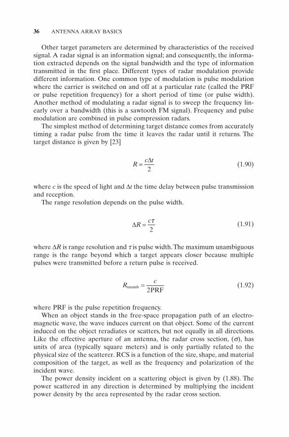
ANTENNA ARRAY APPLICATIONS 37
P
PG LR
st t t= σπ4 2
(1.93)
If the scattered power travels a distance R r to receive with a gain of G r , then the fi nal equation for the received power (Figure 1.21 ) is
P
PG L A LR R
st t t e r
t r
= σπ16 2 2 2
(1.94)
This equation is known as the bistatic radar range equation because the trans-mitter and receiver are at two different locations [24] .
Like an antenna pattern, the RCS pattern has a main lobe, sidelobes, and nulls. Also like antenna patterns, two - dimensional plots are frequently used to evaluate various properties of RCS. Since RCS has units of m 2 , when expressed in logarithmic form it is usually compared to a 1 - m 2 target. Thus, the units are dBsm or dB relative to a square meter.
When the radar uses one antenna to transmit and receive, the bistatic radar range equation reduces to the monostatic radar range equation or more simply the radar range equation. The RCS in this case represents only power scat-tered directly back to the radar (backscattering). For clarity, the path loss ( L ) has been ignored.
PPGA
R
PG
Rr
t e t=( )
=( )
σπ
λ σπ4 42 2
2 2
3 4
(1.95)
Example. An over - the - horizon radar transmits a pulse with 1 - MW average power. This waveform bounces from the ionosphere to the ocean and back to a receive station that is 300 miles away from the transmit station. If the distance from the transmitter to the ocean is 2000 km and the distance
Figure 1.21. Derivation of the bistatic radar range equation.

38 ANTENNA ARRAY BASICS
from the ocean to the receive antenna is 2400 km, then how much power arrives at the receiver. Both the transmit and receive antennas have gains of 30 dB. The bistatic RCS of the ocean at these angles is 10 m 2 . The radar operates at 10 MHz. G = 10 30/10 = 1000, λ = 3 × 10 8 /(10 × 10 6 ) = 30.0 m, A e = 30 2 (1000)/(4 π ) = 71,620.0 m 2 , P r = 1 × 10 6 (1000)(71,620)(10)/[(4 π · 2,000,000) 2 (4 π · 2,400,000) 2 ] = 1.2466 × 10 − 15 W
1.5.3. Radiometer
Communications and radar systems use both transmitting and receiving sub-systems. A radiometer, on the other hand, uses only the receiver subsystem [25] . The radiometer listens to electromagnetic waves naturally emitted by objects. All objects with a temperature above absolute zero have vibrating charges. Because accelerating charges radiate electromagnetic waves, the random thermal motion of charges in any object results in the radiation of electromagnetic waves. Temperature indicates the amount of random molecu-lar motion. At higher temperatures, more molecular collisions take place, and molecules move faster because more energy is stored in the material; there-fore, more waves will be radiated at higher frequencies. Thus, temperature and electromagnetic radiation are closely related.
A blackbody is a perfect radiator and absorber of electromagnetic energy. Planck ’ s radiation law states that a blackbody radiates uniformly in all direc-tions with a spectral brightness given by
B
hfc e
f hf k TB=
−⎛⎝
⎞⎠
2 11
3
2
(1.96)
where B f is spectral brightness, h is Planck ’ s constant, f is temporal frequency (Hz), c is the speed of light in a vacuum (3 × 10 8 m/s), k B = Boltzman ’ s constant (1.23 × 10 − 23 JK − 1 ), and T is absolute temperature (K). This power is radiated over a broad range of frequencies; but for objects with temperatures near the ambient reference temperature (300 K), most of the power is concentrated in the thermal infrared region of the electromagnetic spectrum. At microwave frequencies, although these signals are only about one - millionth as strong as the thermal infrared signal, good microwave antenna systems can detect the blackbody radiation. The brightness is found by integrating the blackbody spectral brightness over a frequency bandwidth ( f ) for a blackbody at tem-perature T . This equation is known as the Stefan – Boltzmann law:
B B df Tf
s= =∞
∫0
4σπ
(1.97)
where σ s = 5.673 × 10 − 8 Wm − 2 K − 4 is the Stefan – Boltzmann constant. No natural objects emit perfect blackbody radiation; however, all objects such as terrain, sea, or the atmosphere emit a fraction of the ideal thermal radiation. The

ANTENNA ARRAY APPLICATIONS 39
emissivity ( e ) is the ratio of the brightness of an object to the brightness of a blackbody at the same temperature.
e
BBbb
θ φ θ φ,
,( ) = ( )
(1.98)
where B( θ , φ ) represents brightness of material at temperature T and B bb represents brightness of a blackbody at temperature T . Emissivity ranges between zero for a perfect refl ector to unity for a blackbody. Emissivity varies with the material composition and the shape of the radiating object as well as with wavelength. At some frequencies, a particular body looks a lot more like a blackbody than at other frequencies.
Brightness temperature, T B , is another way to represent the thermal radia-tion emitted from a gray body. For a blackbody, the temperature equals the absolute temperature of the object. Note that the emissivity and brightness temperature vary with orientation.
T e TB θ φ θ φ, ,( ) = ( ) (1.99)
The output of an antenna receiving only thermal radiation is frequently rep-resented by an antenna temperature, T A , which is proportional to the total power resulting from the thermal radiation incident on the antenna. The antenna temperature is given by
T T G dA B= ( ) ( )∫∫
14 4π
θ φ θ φπ
, , Ω
(1.100)
where G ( θ , φ ) is the antenna gain pattern and T B ( θ , φ ) is the brightness tem-perature distribution incident on the antenna, and d Ω is the differential solid angle. The antenna temperature is therefore the spatially fi ltered sum of the radiation emitted by the bodies surrounding the antenna.
A receiving antenna generates power due to the increased thermal activity. If the antenna is modeled as a noise - generating resistor at temperature, T A , the available noise power from the antenna is given by
P k T fr B A= Δ (1.101)
where k B = 1.23 × 10 − 23 J K − 1 J (Boltzmann ’ s constant) and Δ f is the bandwidth of the receiver. A radiometer uses an antenna and receiving system to measure emission from objects. The brightness temperature distribution incident on a spaceborne microwave radiometer directed toward the earth is due both to radiation from the earth ’ s surface and its atmosphere. At microwave frequen-cies below 10 GHz, atmospheric absorption and emission is small and may be neglected. At higher frequencies, the atmospheric contributions are signifi cant and must be included.

40 ANTENNA ARRAY BASICS
Since emissivity is a characteristic of target size, shape, and composition, the brightness temperature for any aspect maps the emissivity of the observed target to a power level. The radiometer uses a highly directional antenna to scan in azimuth and elevation, and the data are recorded to produce a pixel map of the emissivity of the surface being scanned.
Example. Calculate the power received by an isotropic point source if the emissivity of the observed object is isotropic at 300 K.
First, fi nd T T d dA A: = ( )( )( )∫∫1
41 300 1
00
2
πθ θ φππ
sin and then substitute into
(1.101) to get P r = 300 × 1.23 × 10 − 23 × Δ f .
1.5.4. Electromagnetic Heating
Electromagnetic heating systems radiate electromagnetic waves for the sole purpose of heating an object. When an electromagnetic wave strikes an object, it induces both a displacement current and a conduction current. Conduction current results from the free movement of electrons in an object, while dis-placement current results from the constrained motion of electric dipoles, a polarized pair of charges. If the material has high conductivity, conduction current predominates, and the surface current density is expressed by Ohm ’ s law,
J Eσ σ= (1.102)
If the material has a large real - valued dielectric constant, most of the induced current will be a displacement current density equal to the time rate of change of the electric fl ux density ( D ).
J
Dε = ∂
∂t (1.103)
The total current density is the sum of the displacement current density and the conduction current density.
J J J
DET
t= + = ∂
∂+ε σ σ
(1.104)
Ordinarily, charged particles and dipoles are randomly distributed and oriented in a media, so the thermal activity is totally random. An electric fi eld, however, induces organized motion of charges (current). A time - varying fi eld causes free electrons, ions, and dipoles to move in a target. They collide and transfer some of their energy to other particles. Since molecular dipoles have larger mass than electrons, heating is more effective in dielectrics, where dis-
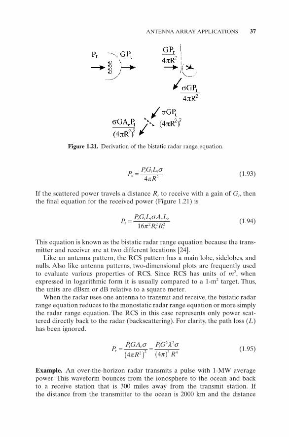
ANTENNA ARRAY APPLICATIONS 41
placement current is large. The fi eld induces a torque on the dipoles that makes each molecule attempt to rotate in order to align its dipole moment with the electric fi eld. For instance, water molecules, which are dipoles, become polarized by an applied electric fi eld (Figure 1.22 ). Due to the inertia of the molecule, it takes time for this torque to polarize the media. Energy is transferred to surrounding molecules and the dipoles rotate, thereby increas-ing the temperature. Conversely, when the electric fi eld is removed, the increased random molecular motion destroys the alignment of the dipole moments and reduces the polarization exponentially with time.
The response time of a dielectric is a measure of the rate at which the polarization decays if the electric fi eld is suddenly removed. The amount of displacement current density is time - dependent. Some of the dipole alignment energy becomes random motion (heat) every time a dipole is knocked out of alignment and then realigned. The response time indicates whether the dipole moments can keep in step with a time - varying electric fi eld. At low frequencies the electric fi elds change direction slower than the response time of the dipoles, so the dipoles orient quickly, and the media only absorbs energy for a rela-tively short period of time. If the electric fi eld changes direction faster than the response time of the dipoles, the dipoles do not rotate, no energy is absorbed, and the dielectric does not heat. When the electric fi eld changes at about the same rate that the dipoles can respond, they rotate, but the resulting
+ +_
++ _
+ +_
++ _++ _
++
_+
+_
++
_ ++
_ ++
_ ++
_
++
_+
+_
++_ ++_
no field
++ _++ _
++ _++ _
++ _++ _
++ _++ _
++ _++ _
++ _++ _
E
applied electric field
Figure 1.22. Water molecules aligning with the electric fi eld.
42 ANTENNA ARRAY BASICS
polarization lags behind the changes in the direction of the electric fi eld. This lag indicates that the dielectric absorbs energy from the fi eld and its tempera-ture increases [26] .
A microwave heating system consists of a microwave source and antenna. The source generates power at a frequency selected to correspond to the response time of the dielectric being heated. Heating of dielectrics has two familiar applications: microwave ovens and cancer therapy (induced hyper-thermia). These applications work because both food and tumors contain mostly water (a molecular dipole). The heater uses an appropriate frequency (high MHz to low GHz region) to excite the water dipoles at a rate near the response time of water, and the target absorbs the transmitted energy.
Example. If a microwave oven is placed in a room at a temperature less than 0 ° C, can the oven melt an ice cube?
Answer: As explained above, the microwave oven excites dipoles in the water. Ice is a crystal. Consequently, the ice will not melt. If there is a small amount of water on the ice, then this water will heat and the ice will melt through microwave heating of the water and heat conduction.
1.5.5. Direction Finding
Finding the direction of a signal can be done in two ways. The fi rst is to point the antenna main beam at the signal, so the direction of the signal occurs at the maximum received power. This approach requires a large antenna for accurate direction fi nding. On the other hand, nulls are precisely defi ned and have large variations in gain over a short angular sector. A small loop has a distinct null that has been used for direction fi nding since the early 1900s. Figure 1.23 shows an example of an early DF loop antenna that operated at HF.
1.6. ORGANIZATION AND OVERVIEW
This book is organized as a progression from relatively simple antenna arrays consisting of point sources to very complex digital beamforming arrays that can perform extremely complex signal processing. Most research on arrays was limited to point sources due to the computational limits of computers. The next two chapters summarize many of the developments surrounding the analysis and synthesis of these simple arrays. Real antenna arrays have real antenna elements, however. These elements are introduced in Chapter 4 . Chapter 5 extends the narrow view of an array lying in a plane to an array consisting of antenna elements that can lie anywhere on a surface or in space. Thus, an array becomes even more versatile than a single aperture antenna. Placing array elements close together results in the elements interacting with each other. Each element in the array receives signals for all the other ele-

REFERENCES 43
ments in the array. This mutual coupling can signifi cantly change the array performance and must be accounted for in the design. This complicated mutual coupling concept is described in Chapter 6 . Coherently combining the signals in an array or beamforming is addressed in Chapter 7 . Finally, the array has the potential to change its ability to receive and transmit signals based upon the environment and feedback. These adaptive arrays can reject interfer-ence, form multiple beams, and change performance characteristics. An emphasis is placed upon computational aspects of antenna arrays.
REFERENCES
1. J. A. Fleming , The Principles of Electric Wave Telegraphy and Telephony , 3rd ed ., New York : Longmans, Green, and Co. , 1916 .
2. S. G. Brown , British Patent No. 14,449 , 1899 . 3. L. De Forest , Wireless - signaling apparatus, U.S. Patent 749,131 , January 5, 1904 . 4. G. Marconi , On methods whereby the radiation of electic waves may be mainly
confi ned to certain directions, and whereby the receptivity of a receiver may be
Figure 1.23. Early DF loop antenna. (Courtesy of the National Electronics Museum.)
44 ANTENNA ARRAY BASICS
restricted to electric waves emanating from certain directions , Proc. R. Soc. Lond. Ser. A, Vol. 77 , 1906 , p. 413 .
5. G. Goebel , The British invention of radar , v2.0.3 / chapter 1 of 12 / 01 may 09 / greg goebel / public domain , http://www.vectorsite.net/ttwiz_01.html#m2 .
6. S. N. Stitzer , The SCR - 270 radar , IEEE Microwave Mag. , Vol. 8 , No. 3 , June 2007 , pp. 88 – 98 .
7. F. Braun , Directed wireless telegraphy , The Electrician , Vol. 57 , May 25, p. 222 . 8. H. T. Friis , A new directional receiving system , IRE Proc. , Vol. 13 , No. 6 , December
1925 , pp. 685 – 707 . 9. H. T. Friis , C. B. Feldman , and W. M. Sharpless , The determination of the direc-
tion of arrival of short radio waves , IRE Proc. , Vol. 22 , No. 1 , January 1934 , pp. 47 – 77 .
10. G. H. Brown , Directional antennas , IRE Proc. , Vol. 25 , No. 1 , Part 1, January 1937 , pp. 78 – 145 .
11. H. T. Friis and C. B. Feldman , A multiple unit steerable antenna for short - wave reception , IRE Proc . , Vol. 25 , No. 7 , July 1937 , pp. 841 – 917 .
12. J. L. Spradley , A volumetric electrically scanned two - dimensional microwave antenna array , IRE Int. Convention Record , Vol. 6 , Part 1, March 1958 , pp. 204 – 212 .
13. S. A. Schelkunoff , A mathematical theory of linear arrays , Bell Syst. Tech. J. , Vol. 22 , 1943 , pp. 80 – 107 .
14. C. L. Dolph , A current distribution for broadside arrays which optimizes the rela-tionship between bream width and side - lobe level , Proc. IRE , Vol. 34 , June 1946 , pp. 335 – 348 .
15. S. P. Applebaum , Adaptive arrays , Syracuse University Research Corporation Report SPL TR 66 - 1, August 1966 .
16. R. J. Mallioux , A history of phased array antennas , in History of Wireless , T. K. Sarkar et al., ed., New York : John Wiley & Sons , 2006 , pp. 567 – 604 .
17. E. Brookner , Phased - array radars: Pase, astounding breakthroughs and future trends , Microwave J. , Vol. 51 , No. 1 , January 2008 , pp. 30 – 50 .
18. A brief history of the sea - based X - band radar - 1 , Missile Defense Agency History Offi ce, May 1, 2008 .
19. IEEE standard defi nitions of terms for antennas , IEEE AP Trans . , AP - 31, No. 6, November 1993 .
20. H. Schantz , Ultrawideband Antennas , Norwood, MA : Artech House , 2005 . 21. J. D. Kraus , Antennas , 2nd ed ., McGraw - Hill , New York , 1988 . 22. H. T. Friis , A note on a simple transmission formula , IRE Proc . , Vol. 33 , No. 2 ,
May 1946 , pp. 254 – 256 . 23. G. W. Stimson , Introduction to Airborne Radar , Hughes Aircraft Co. , El Segundo,
CA , 1983 . 24. M. I. Skolnik , Introduction to Radar Systems , New York : McGraw - Hill , 2002 . 25. F. T. Ulaby , R. K. Moore , and A. K. Fung , Microwave Remote Sensing: Active and
Passive , Vol. II , Reading, MA : Addison - Wesley , 1982 . 26. J. Walker , The secret of a microwave oven ’ s rapid cooking action is disclosed , Sci.
Am. , February 1987 , pp. 134 – 138 .