1

Binary Image B(r,c)

2

0 represents the background 1 represents the foreground

000100100010000001111000100000010010001000

Binary Image Analysis is used in a number of

practical applications, e.g.

3

• Part inspection

• Shape analysis

• Enhancement

• Document processing

What kinds of operations?

4

Separate objects from background and from one another

Aggregate pixels for each object

Compute features for each object

Example: red blood cell image Many blood cells are

separate objects Many touch – bad! Salt and pepper

noise from thresholding

How useable is this data?

5

Results of analysis 63 separate

objects detected

Single cells have area about 50

Noise spots Gobs of cells

6

Binary Image Operations

7

1. Thresholding a gray-tone image2. Convolution3. Morphology4. Feature extractions (area, centroid) 5. Connected components analysis

1. Thresholding

8

•Convert gray level or color image into binary image•Use histogram•Definition: The Histogram of a gray-level image I is defined as

H(m) = { (r,c) : I(r,c) =m) }

Where m spans the gray values

Histogram-Directed Thresholding

9

How can we use a histogram to separate animage into 2 (or several) different regions?

Is there a single clear threshold? 2? 3?

Histogram

Background is black Healthy cherry is bright Bruise is medium dark Histogram shows two

cherry regions (black background has been removed)

10

gray-tone values

pixelcounts

0 256

Automatic Thresholding: Otsu’s Method

11

Assumption: the histogram is bimodal

t

Method: find the threshold t that minimizesthe weighted sum of within-group variancesfor the two groups that result from separatingthe gray tones at value t.

Grp 1 Grp 2

Thresholding Example

12

original gray tone image binary thresholded image

2. Convolution Given a gray level image I(r,c) and a mask m(r,c)

convolution is

I(r,c)*m(r,c)= ΣΣ I(k,l) . m(r-k,m-l)

13

Masks

SMOOTHING MASKS

Convolution of an İmage with a Mask

15

Image Enhancement WITH AVERAGING AND THRESHOLDING

Image Enhancement WITH AVERAGING AND THRESHOLDING

3. Mathematical Morphology Morphology: Study of forms of animals

and plants Mathematical Morphology: Study of

shapes Similar to convolution Arithmetic operations Set Operations

18

Need to define Image as a Set Given a binary image I (r,c), assume 1

correspond to object 0 correspond to backround.

Define a set with elements to the coordinates of the object

X = { (r1,c1), (r2,c2),….}

19

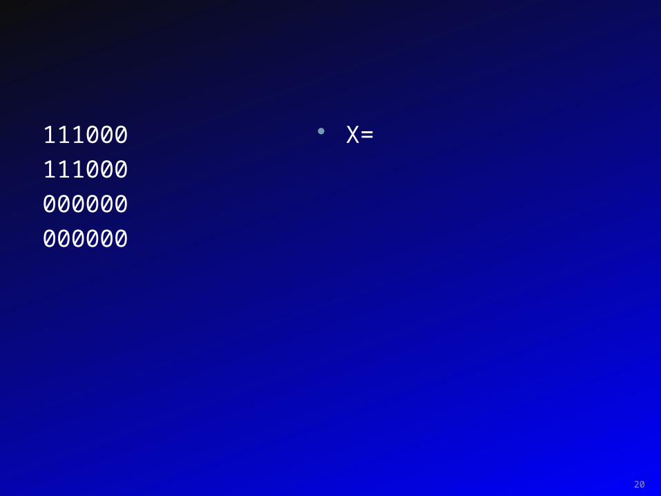
111000

111000

000000

000000

X=

20

Set OperationsSet Operations

Set Operations on ImagesSet Operations on ImagesAND, ORAND, OR

Set Operations on ImagesSet Operations on ImagesAND, ORAND, OR

TRANSLATION REFLECTIONTRANSLATION REFLECTIONTRANSLATION REFLECTIONTRANSLATION REFLECTION

Set OperationsSet Operations

Morphologic Operations

25

Binary mathematical morphology consists of twobasic operations

dilation and erosion

and several composite relations

closing and opening

Dilation:

26

Dilation expands the connected sets of 1s of a binary image.

It can be used for

1. growing regions

2. filling holes and gaps

Structuring Elements

27

A structuring element is a shape mask used inthe basic morphological operations.

They can be any shape and size that isdigitally representable, and each has an origin.

boxhexagon disk

something

box(length,width) disk(diameter)

Dilation with Structuring Element S: ={ Z: (Sz)∩ B≠ Φ}

28

The arguments to dilation and erosion are

1. a binary image B2. a structuring element S

dilate(B,S) takes binary image B, places the originof structuring element S over each 1-pixel, and ORsthe structuring element S into the output image atthe corresponding position.

0 0 0 00 1 1 00 0 0 0

11 1

0 1 1 00 1 1 10 0 0 0

originBS

dilate

B S

B S

DILATIONDILATION

DILATIONDILATION

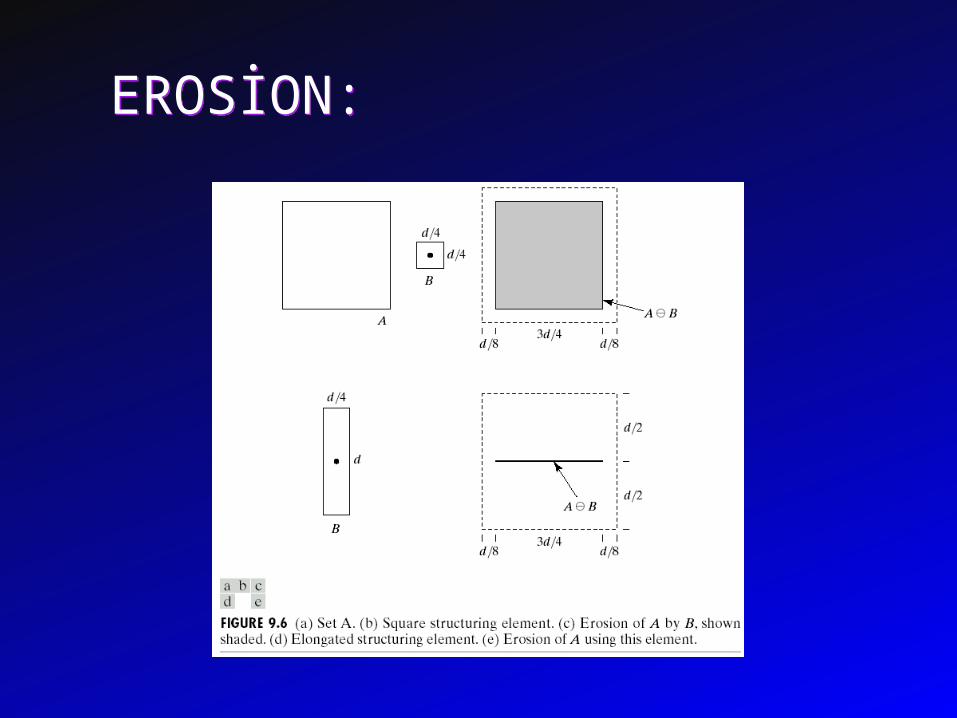
Erosion BΘS ={ Z: (Sz) B}

31

Erosion shrinks the connected sets of 1s of a binary image.

It can be used for

1. shrinking features

2. Removing bridges, branches and small protrusions

Erosion with Structuring Elements

32

erode(B,S) takes a binary image B, places the origin of structuring element S over every pixel position, andORs a binary 1 into that position of the output image only ifevery position of S (with a 1) covers a 1 in B.

0 0 1 1 00 0 1 1 00 0 1 1 01 1 1 1 1

111

0 0 0 0 00 0 1 1 00 0 1 1 00 0 0 0 0

B S

origin

erode

B S

EROSİON:EROSİON:

IMAGE ENHANCEMENT WİTH MORPHOLOGYIMAGE ENHANCEMENT WİTH MORPHOLOGY

Example to Try

35

0 0 1 0 0 1 0 0 0 0 1 1 1 1 1 0 1 1 1 1 1 1 0 01 1 1 1 1 1 1 10 0 1 1 1 1 0 0 0 0 1 1 1 1 0 0 0 0 1 1 1 1 0 0

1 1 11 1 11 1 1

erode

dilate with same structuring element

SB

Opening and Closing

36

• Closing is the compound operation of dilation followed by erosion (with the same structuring element)

• Opening is the compound operation of erosion followed by dilation (with the same structuring element)

Use of Opening

37

Original Opening Corners

1. What kind of structuring element was used in the opening?

2. How did we get the corners?

OPENİNG AND CLOSİNGOPENİNG AND CLOSİNGOPENİNG AND CLOSİNGOPENİNG AND CLOSİNG

FINGERPRİNT RECOGNİTİONFINGERPRİNT RECOGNİTİON

HOW DO YOU REMOVE THE HOLESHole: A closed backround region surrounded by object pixels

HOW DO YOU REMOVE THE HOLESHole: A closed backround region surrounded by object pixels

41

Erode with hole ring and dilate with hole mask

Morphological Analysis for Bone detectionMorphological Analysis for Bone detection

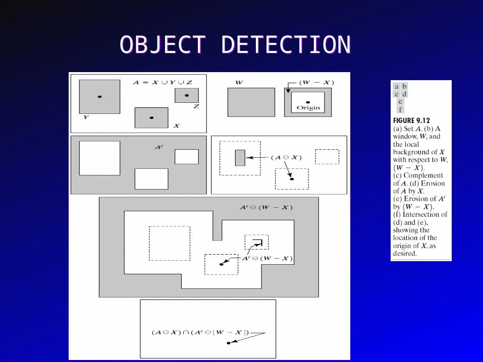
OBJECT DETECTIONOBJECT DETECTION

BOUNDARY EXTRACTİONBoundary: A set of one-pixel-wide

connected pixels which has at least one neighbor outside the object

BOUNDARY EXTRACTİONBoundary: A set of one-pixel-wide

connected pixels which has at least one neighbor outside the object

BOUNDARY EXTRACTİONBOUNDARY EXTRACTİON

Skeleton FindingSkeleton: Set of one-pixel wide connected pixels which

are at equal distance from at least two boundary pixels

Skeleton FindingSkeleton: Set of one-pixel wide connected pixels which

are at equal distance from at least two boundary pixels

Morphological Image ProcessingMorphological Image Processing

Morphological OperationsMorphological Operations

Morphological OperationsMorphological Operations

Skeleton finding:Skeleton: Set of one-pixel wide connected pixels which

are at equal distance from at least two boundary pixels

Skeleton finding:Skeleton: Set of one-pixel wide connected pixels which

are at equal distance from at least two boundary pixels

Gear Tooth Inspection

52

originalbinary image

detecteddefects

How didthey do it?

Some Details

53

Region Properties-Features

54

Properties of the regions can be used to recognize objects.

• geometric properties (Ch 3)

• gray-tone properties

• color properties

• texture properties

• shape properties (a few in Ch 3)

• motion properties

• relationship properties (1 in Ch 3)

Geometric and Shape Properties

55

• area:

• centroid:

• perimeter :

• perimeter length:

• circularity:

• elongation• mean and standard deviation of radial

distance• bounding box• extremal axis length from bounding

box• second order moments (row, column,

mixed)• lengths and orientations of axes of

best-fit ellipse

56

4. Connected Components Labeling

57

Once you have a binary image, you can identify and then analyze each connected set of pixels.

The connected components operation takes in a binary image and produces a labeled image in which each pixel has the integer label of either the background (0) or a component.

binary image after morphology connected components

Methods for CC Analysis

58

1. Recursive Tracking (almost never used)

2. Parallel Growing (needs parallel hardware)

3. Row-by-Row (most common)

• Classical Algorithm (see text)

• Efficient Run-Length Algorithm (developed for speed in real industrial applications)

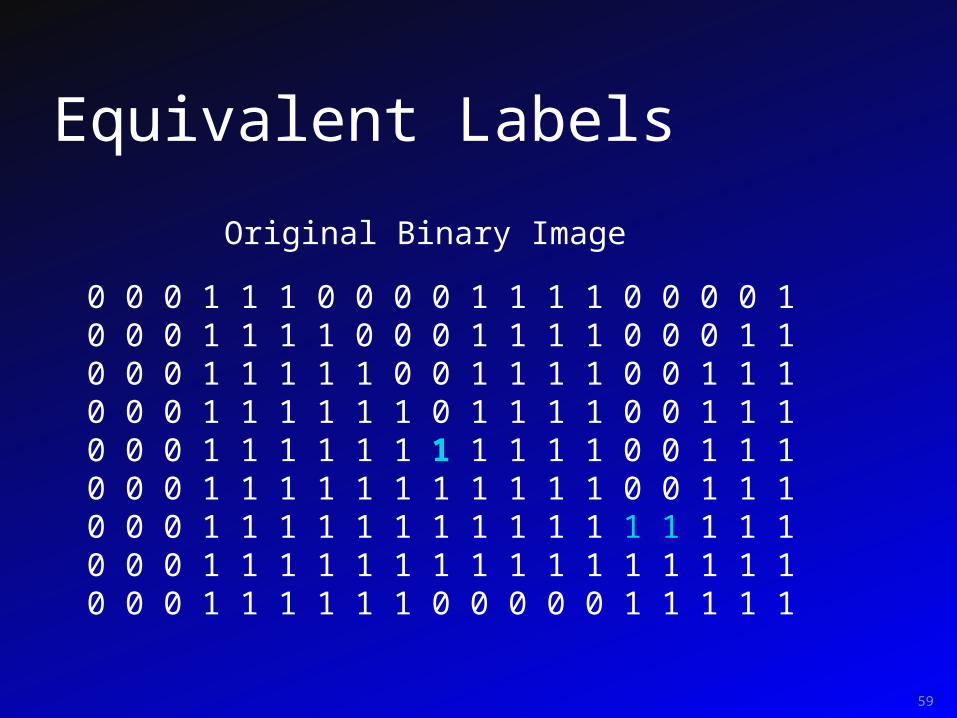
Equivalent Labels

59

0 0 0 1 1 1 0 0 0 0 1 1 1 1 0 0 0 0 10 0 0 1 1 1 1 0 0 0 1 1 1 1 0 0 0 1 10 0 0 1 1 1 1 1 0 0 1 1 1 1 0 0 1 1 10 0 0 1 1 1 1 1 1 0 1 1 1 1 0 0 1 1 10 0 0 1 1 1 1 1 1 1 1 1 1 1 0 0 1 1 10 0 0 1 1 1 1 1 1 1 1 1 1 1 0 0 1 1 10 0 0 1 1 1 1 1 1 1 1 1 1 1 1 1 1 1 10 0 0 1 1 1 1 1 1 1 1 1 1 1 1 1 1 1 10 0 0 1 1 1 1 1 1 0 0 0 0 0 1 1 1 1 1

Original Binary Image

Equivalent Labels

60

0 0 0 1 1 1 0 0 0 0 2 2 2 2 0 0 0 0 30 0 0 1 1 1 1 0 0 0 2 2 2 2 0 0 0 3 30 0 0 1 1 1 1 1 0 0 2 2 2 2 0 0 3 3 30 0 0 1 1 1 1 1 1 0 2 2 2 2 0 0 3 3 30 0 0 1 1 1 1 1 1 1 1 1 1 1 0 0 3 3 30 0 0 1 1 1 1 1 1 1 1 1 1 1 0 0 3 3 30 0 0 1 1 1 1 1 1 1 1 1 1 1 1 1 1 1 10 0 0 1 1 1 1 1 1 1 1 1 1 1 1 1 1 1 10 0 0 1 1 1 1 1 1 0 0 0 0 0 1 1 1 1 1

The Labeling Process

1 21 3

Run-Length Data Structure

61

1 1 1 11 1 11 1 1 1

1 1 1 1

0 1 2 3 401234

U N U S E D 00 0 1 00 3 4 01 0 1 01 4 4 02 0 2 02 4 4 04 1 4 0

row scol ecol label

01234567

Rstart Rend

1 23 45 60 07 7

01234 Runs

Row Index

BinaryImage

Run-Length Algorithm

62

Procedure run_length_classical { initialize Run-Length and Union-Find data structures count <- 0

/* Pass 1 (by rows) */

for each current row and its previous row { move pointer P along the runs of current row move pointer Q along the runs of previous row

Case 1: No Overlap

63

|/////| |/////| |////|

|///| |///| |/////|

Q

P

Q

P

/* new label */ count <- count + 1 label(P) <- count P <- P + 1

/* check Q’s next run */Q <- Q + 1

Case 2: Overlap

64

Subcase 1: P’s run has no label yet

|///////| |/////| |/////////////|

Subcase 2:P’s run has a label that isdifferent from Q’s run

|///////| |/////| |/////////////|

QQ

P P

label(P) <- label(Q)move pointer(s)

union(label(P),label(Q))move pointer(s)

}

Pass 2 (by runs)

65

/* Relabel each run with the name of the equivalence class of its label */For each run M { label(M) <- find(label(M)) }

}

where union and find refer to the operations of theUnion-Find data structure, which keeps track of setsof equivalent labels.

Labeling shown as Pseudo-Color

66

connectedcomponentsof 1’s fromthresholdedimage

connectedcomponentsof clusterlabels

Region Adjacency Graph

67

A region adjacency graph (RAG) is a graph in whicheach node represents a region of the image and an edgeconnects two nodes if the regions are adjacent.

1

2

34

1 2

34