1

Biological Sequence Analysis

BioInfoSummer@ANU, Dec 2 2003

Terry SpeedUniversity of California at Berkeley

& WEHI Melbourne

2

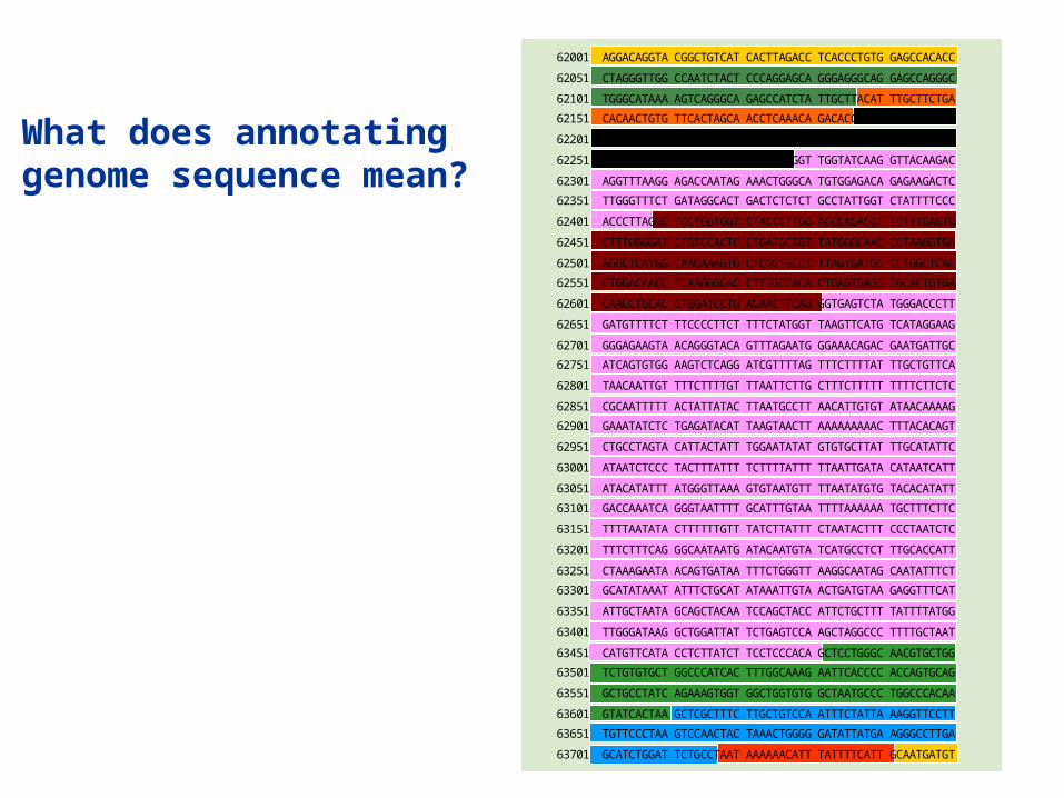
Annotating Genome Sequence

This is one of the most challenging and interesting

problems in computational biology at the moment.

3

62001 AGGACAGGTA CGGCTGTCAT CACTTAGACC TCACCCTGTG GAGCCACACC

62051 CTAGGGTTGG CCAATCTACT CCCAGGAGCA GGGAGGGCAG GAGCCAGGGC

62101 TGGGCATAAA AGTCAGGGCA GAGCCATCTA TTGCTTACAT TTGCTTCTGA

62151 CACAACTGTG TTCACTAGCA ACCTCAAACA GACACCATGG TGCACCTGAC

62201 TCCTGAGGAG AAGTCTGCCG TTACTGCCCT GTGGGGCAAG GTGAACGTGG

62251 ATGAAGTTGG TGGTGAGGCC CTGGGCAGGT TGGTATCAAG GTTACAAGAC

62301 AGGTTTAAGG AGACCAATAG AAACTGGGCA TGTGGAGACA GAGAAGACTC

62351 TTGGGTTTCT GATAGGCACT GACTCTCTCT GCCTATTGGT CTATTTTCCC

62401 ACCCTTAGGC TGCTGGTGGT CTACCCTTGG ACCCAGAGGT TCTTTGAGTC

62451 CTTTGGGGAT CTGTCCACTC CTGATGCTGT TATGGGCAAC CCTAAGGTGA

62501 AGGCTCATGG CAAGAAAGTG CTCGGTGCCT TTAGTGATGG CCTGGCTCAC

62551 CTGGACAACC TCAAGGGCAC CTTTGCCACA CTGAGTGAGC TGCACTGTGA

62601 CAAGCTGCAC GTGGATCCTG AGAACTTCAG GGTGAGTCTA TGGGACCCTT

62651 GATGTTTTCT TTCCCCTTCT TTTCTATGGT TAAGTTCATG TCATAGGAAG

62701 GGGAGAAGTA ACAGGGTACA GTTTAGAATG GGAAACAGAC GAATGATTGC

62751 ATCAGTGTGG AAGTCTCAGG ATCGTTTTAG TTTCTTTTAT TTGCTGTTCA

62801 TAACAATTGT TTTCTTTTGT TTAATTCTTG CTTTCTTTTT TTTTCTTCTC

62851 CGCAATTTTT ACTATTATAC TTAATGCCTT AACATTGTGT ATAACAAAAG

62901 GAAATATCTC TGAGATACAT TAAGTAACTT AAAAAAAAAC TTTACACAGT

62951 CTGCCTAGTA CATTACTATT TGGAATATAT GTGTGCTTAT TTGCATATTC

63001 ATAATCTCCC TACTTTATTT TCTTTTATTT TTAATTGATA CATAATCATT

63051 ATACATATTT ATGGGTTAAA GTGTAATGTT TTAATATGTG TACACATATT

63101 GACCAAATCA GGGTAATTTT GCATTTGTAA TTTTAAAAAA TGCTTTCTTC

63151 TTTTAATATA CTTTTTTGTT TATCTTATTT CTAATACTTT CCCTAATCTC

63201 TTTCTTTCAG GGCAATAATG ATACAATGTA TCATGCCTCT TTGCACCATT

63251 CTAAAGAATA ACAGTGATAA TTTCTGGGTT AAGGCAATAG CAATATTTCT

63301 GCATATAAAT ATTTCTGCAT ATAAATTGTA ACTGATGTAA GAGGTTTCAT

63351 ATTGCTAATA GCAGCTACAA TCCAGCTACC ATTCTGCTTT TATTTTATGG

63401 TTGGGATAAG GCTGGATTAT TCTGAGTCCA AGCTAGGCCC TTTTGCTAAT

63451 CATGTTCATA CCTCTTATCT TCCTCCCACA GCTCCTGGGC AACGTGCTGG

63501 TCTGTGTGCT GGCCCATCAC TTTGGCAAAG AATTCACCCC ACCAGTGCAG

63551 GCTGCCTATC AGAAAGTGGT GGCTGGTGTG GCTAATGCCC TGGCCCACAA

63601 GTATCACTAA GCTCGCTTTC TTGCTGTCCA ATTTCTATTA AAGGTTCCTT

63651 TGTTCCCTAA GTCCAACTAC TAAACTGGGG GATATTATGA AGGGCCTTGA

63701 GCATCTGGAT TCTGCCTAAT AAAAAACATT TATTTTCATT GCAATGATGT

What does annotating genome sequence mean?

4

Synopsis

Some biological backgroundA progression of modelsAcknowledgementsReferences

5

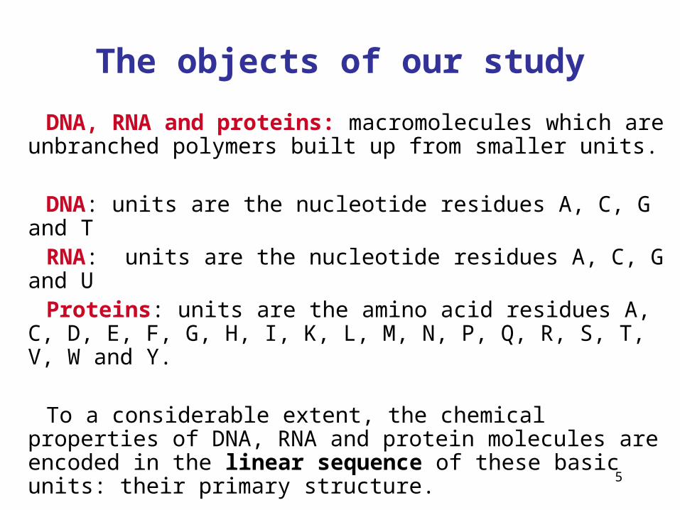
The objects of our study

DNA, RNA and proteins: macromolecules which are unbranched polymers built up from smaller units.

DNA: units are the nucleotide residues A, C, G and T RNA: units are the nucleotide residues A, C, G and U Proteins: units are the amino acid residues A, C, D, E,

F, G, H, I, K, L, M, N, P, Q, R, S, T, V, W and Y.

To a considerable extent, the chemical properties of DNA, RNA and protein molecules are encoded in the linear sequence of these basic units: their primary structure.

6

The central dogma

Protein

mRNA

DNA

transcription

translation

CCTGAGCCAACTATTGATGAA

PEPTIDE

CCUGAGCCAACUAUUGAUGAA

7

A protein-coding gene

8

Motifs - Sites - Signals - Domains

For this talk, I’ll use these terms interchangeably to describe recurring elements of interest to us.

In PROTEINS we have: transmembrane domains, coiled-coil domains, EGF-like domains, signal peptides, phosphorylation sites, antigenic determinants, ...

In DNA / RNA we have: enhancers, promoters, terminators, splicing signals, translation initiation sites, centromeres, ...

9

Motifs and models

Motifs typically represent regions of structural significance with specific biological function.

Are generalisations from known examples.

The models can be highly specific.

Multiple models can be used to give higher sensitivity & specificity in their detection.

Can sometimes be generated automatically from examples or multiple alignments.

10

The use of stochastic models for motifs

Can be descriptive, predictive or everything else in between…..almost business as usual.

However, stochastic mechanisms should never be taken literally, but nevertheless they can be amazingly useful.

Care is always needed: a model or method can break down at any time without notice.

Biological confirmation of predictions is almost always necessary.

11

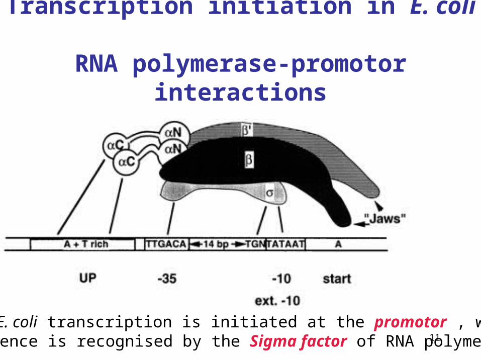
Transcription initiation in E. coli RNA polymerase-promotor interactions

In E. coli transcription is initiated at the promotor , whose sequence is recognised by the Sigma factor of RNA polymerase.

12

Transcription initiation in E. coli, cont.

..YKFSTYATWWIRQAITR..

13

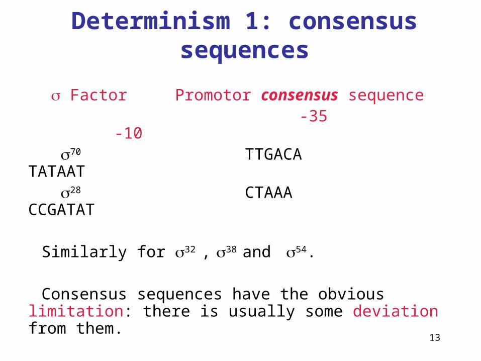
Determinism 1: consensus sequences

Factor Promotor consensus sequence -35 -10 70 TTGACA TATAAT 28 CTAAA CCGATAT Similarly for 32 , 38 and 54. Consensus sequences have the obvious limitation:

there is usually some deviation from them.

14

has 3 Cys-Cys-His-His zinc finger DNA binding domains

The human transcription factor Sp1

15

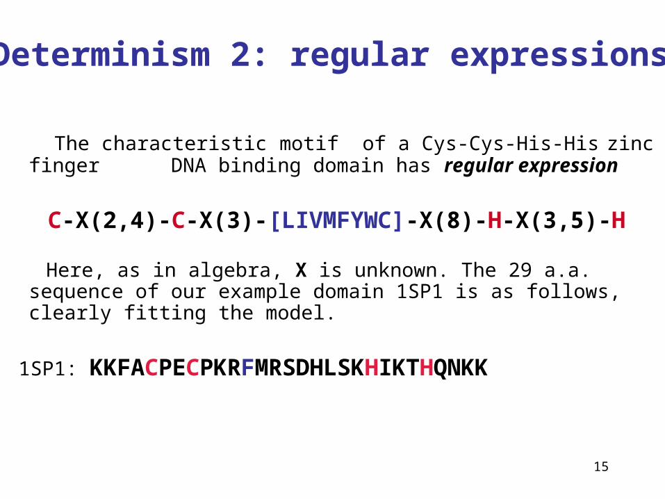
Determinism 2: regular expressions

The characteristic motif of a Cys-Cys-His-His zinc finger DNA binding domain has regular expression

C-X(2,4)-C-X(3)-[LIVMFYWC]-X(8)-H-X(3,5)-H

Here, as in algebra, X is unknown. The 29 a.a. sequence of our example domain 1SP1 is as follows, clearly fitting the model.

1SP1: KKFACPECPKRFMRSDHLSKHIKTHQNKK

16

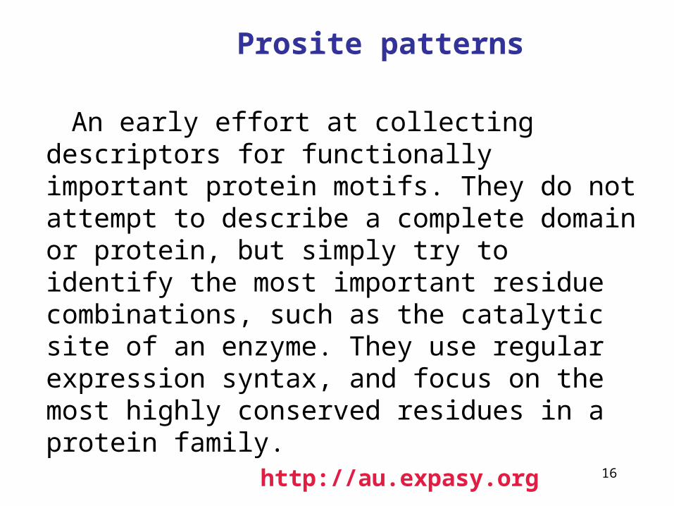
Prosite patterns

An early effort at collecting descriptors for functionally important protein motifs. They do not attempt to describe a complete domain or protein, but simply try to identify the most important residue combinations, such as the catalytic site of an enzyme. They use regular expression syntax, and focus on the most highly conserved residues in a protein family.

http://au.expasy.org

17

More on Prosite patterns

This pattern, which must be in the N-terminal of the sequence (‘<'), means: <A - x - [ST] (2) - x(0,1) - V - {LI} Ala-any- [Ser or Thr]-[Ser or Thr] - (any or none)-Val-(any but Leu, Ile)

18

http://www.isrec.isb-sib.ch/software/PATFND_form.htmlc.{2,4}c...[livmfywc]........h.{3,5}h

PatternFind output[ISREC-Server] Date: Wed Aug 22 13:00:41 MET 2001 ...gp|AF234161|7188808|01AEB01ABAC4F945 nuclear

protein NP94b [Homo sapiens] Occurences: 2 Position : 514 CYICKASCSSQQEFQDHMSEPQH Position : 606 CTVCNRYFKTPRKFVEHVKSQGH........

Searching with regular expressions

19

Regular expressions can be limiting

The regular expression syntax is still too rigid to represent many highly divergent protein motifs.

Also, short patterns are sometimes insufficient with today’s large databases. Even requiring perfect matches you might find many false positives. On the other site some real sites might not be perfect matches.

We need to go beyond apparently equally likely alternatives, and ranges for gaps. We deal with the former first, having a distribution at each position.

20

Cys-Cys-His-His profile: sequence logo form

A sequence logo is a scaled position-specific a.a.distribution. Scaling is by a measure of a position’s information content.

21

Weight matrix model (WMM) = Stochastic consensus sequence

0.04 0.88 0.26 0.59 0.49 0.03

0.09 0.03 0.11 0.13 0.21 0.05

0.07 0.01 0.12 0.16 0.12 0.02

0.80 0.08 0.51 0.13 0.18 0.89

9 214 63 142 118 8

22 7 26 31 52 13

18 2 29 38 29 5

193 19 124 31 43 216

A

C

G

T

A

C

G

T

-38 19 1 12 10 -48

-15 -38 -8 -10 -3 -32

-13 -48 -6 -7 -10 -40

17 -32 8 -9 -6 19

A

C

G

T

2

1

01 2 3 4 5 6

Counts from 242 known 70 sites Relative frequencies: fbl

10log2fbl/pb Informativeness:2+bpbllog2pbl

22

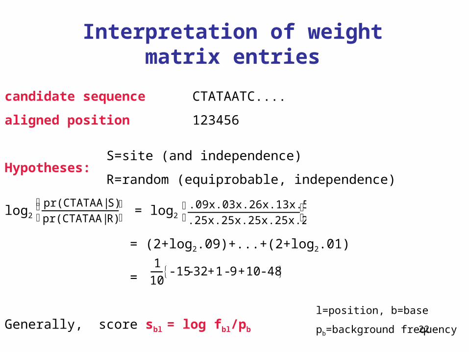
Interpretation of weight matrix entries

candidate sequence CTATAATC....

aligned position 123456

Hypotheses:S=site (and independence)

R=random (equiprobable, independence)

log2 = log2

= (2+log2.09)+...+(2+log2.01)

=

Generally, score sbl = log fbl/pb

pr(CTATAA | S)

pr(CTATAA | R)

⎛ ⎝ ⎜ ⎞

⎠.09x.03x.26x.13x.51x.01

.25x.25x.25x.25x.25x.25 ⎛ ⎝

⎞ ⎠

1

10-15 - 32 +1 - 9 +10 - 48{ }

l=position, b=base

pb=background frequency

23

Use of the matrix to find sites C T A T A A T C

-38 19 1 12 10 -48

-15 -38 -8 -10 -3 -32

-13 -48 -6 -7 -10 -40

17 -32 8 -9 -6 19

A

C

G

T

-38 19 1 12 10 -48

-15 -38 -8 -10 -3 -32

-13 -48 -6 -7 -10 -40

17 -32 8 -9 -6 19

A

C

G

T

-38 19 1 12 10 -48

-15 -38 -8 -10 -3 -32

-13 -48 -6 -7 -10 -40

17 -32 8 -9 -6 19

A

C

G

T

sum

-93

+85

-95

Move the matrixalong the sequenceand score each window.

Peaks should occur at the true sites.

Of course in general any threshold will have some false positive and false negative rate.

24

Transcription Factor Binding Sites

Not much to go on here, see later.

25

Profiles

Are a variation of the position specific scoring matrix approach just described. Profiles are calculated slightly differently to reflect amino acid substitutions, and the possibility of gaps, but are used in the same way.

In general a profile entry Mla for location l and amino acid a is calculated by

Mla = ∑bwlbSab

where b ranges over amino acids, wlb is a weight (e.g. the observed frequency of a.a. b in position l) and Sab is the (a,b)-entry of a substitution matrix (e.g. PAM or BLOSUM) calculated as a likelihood ratio.

Position specific gap penalties can also be included.

26

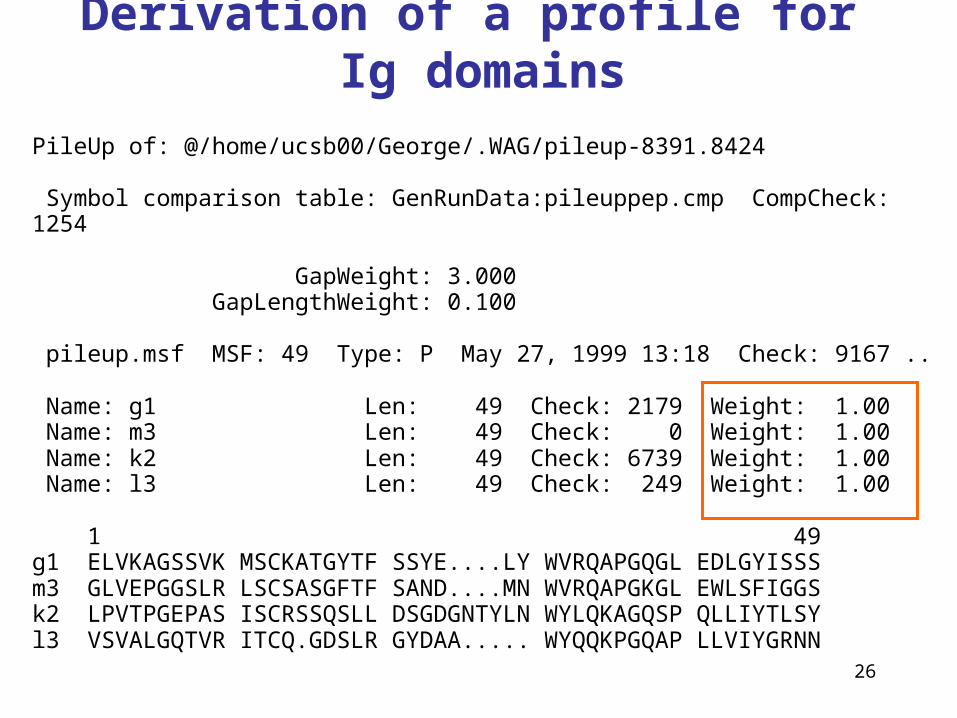
Derivation of a profile for Ig domains

PileUp of: @/home/ucsb00/George/.WAG/pileup-8391.8424

Symbol comparison table: GenRunData:pileuppep.cmp CompCheck:1254

GapWeight: 3.000 GapLengthWeight: 0.100

pileup.msf MSF: 49 Type: P May 27, 1999 13:18 Check: 9167 ..

Name: g1 Len: 49 Check: 2179 Weight: 1.00 Name: m3 Len: 49 Check: 0 Weight: 1.00 Name: k2 Len: 49 Check: 6739 Weight: 1.00 Name: l3 Len: 49 Check: 249 Weight: 1.00

1 49g1 ELVKAGSSVK MSCKATGYTF SSYE....LY WVRQAPGQGL EDLGYISSSm3 GLVEPGGSLR LSCSASGFTF SAND....MN WVRQAPGKGL EWLSFIGGSk2 LPVTPGEPAS ISCRSSQSLL DSGDGNTYLN WYLQKAGQSP QLLIYTLSYl3 VSVALGQTVR ITCQ.GDSLR GYDAA..... WYQQKPGQAP LLVIYGRNN

27

Cons A B C D E F G H I K L M N P Q R S T V W Y Z Gap Len .. V 15 8 -14 14 21 1 24 -4 19 -4 21 19 3 3 8 -14 4 10 32 -33 -14 14 100 100 L 9 -10 -14 -12 -5 24 -3 -6 21 -5 38 34 -9 17 0 -7 14 5 25 9 -7 -4 100 100 V 20 -20 20 -20 -20 20 20 -30 110 -20 80 60 -30 10 -20 -30 -10 20 150 -80 -10 -20 100 100 T 31 21 -10 25 32 -31 21 4 -3 28 -11 0 18 14 17 6 15 32 0 -33 -24 25 100 100 P 35 -1 -4 0 3 -13 12 2 5 -1 10 12 -3 50 11 0 13 14 17 -30 -25 6 100 100 G 70 60 20 70 50 -60 150 -20 -30 -10 -50 -30 40 30 20 -30 60 40 20 -100 -70 30 100 100 E 22 29 -4 36 40 -33 39 10 -12 11 -18 -11 22 15 32 3 31 11 -4 -32 -31 35 100 100 S 25 14 26 11 11 -23 29 -5 -3 11 -18 -12 12 38 0 6 57 34 1 -10 -28 4 100 100 V 26 -11 -1 -9 -6 16 9 -14 46 -11 45 37 -12 6 -5 -19 -3 11 61 -30 -3 -6 100 100 R -4 13 -8 7 7 -30 -3 14 -14 49 -22 5 13 16 17 60 27 4 -14 50 -33 12 100 100! 11 I -1 -17 -13 -19 -13 46 -21 -16 67 -8 64 58 -19 -13 -11 -12 -13 5 54 -13 6 -11 100 100 S 28 20 43 14 14 -21 40 -13 -3 14 -24 -17 20 27 -7 4 90 38 -3 9 -27 1 100 100 C 30 -40 150 -50 -60 -10 20 -10 20 -60 -80 -60 -30 10 -60 -30 70 20 20 -120 100 -60 100 100 K 4 18 -11 17 17 -32 6 15 -12 40 -17 1 17 15 31 39 24 4 -11 18 -31 24 100 100 A 53 11 19 12 12 -20 31 -6 -1 3 -9 -4 11 21 5 -8 33 17 5 -21 -15 6 30 30 S 28 21 28 19 16 -22 45 -11 -5 8 -21 -14 18 21 -2 -2 60 36 2 -13 -27 6 100 100 G 29 41 -9 53 39 -44 60 9 -16 7 -24 -15 28 15 37 -4 20 14 1 -54 -37 37 100 100 W 2 -4 35 -14 -10 31 1 -4 8 -12 8 -4 1 -8 -23 -12 38 1 -2 43 28 -18 100 100 L 10 -10 -19 -10 -3 29 -3 -10 32 -3 44 41 -6 0 -6 -16 -3 44 32 -3 0 -3 100 100 W -21 -28 -18 -39 -26 57 -30 1 29 -15 53 37 -20 -22 -21 -1 -14 -12 13 68 40 -22 100 100! 21 S 27 33 18 37 27 -32 50 -4 -10 9 -27 -19 25 18 9 -1 59 18 -3 -20 -29 17 100 100 S 29 8 40 4 4 3 19 -4 -2 -2 -10 -11 11 9 -9 -9 48 11 -2 14 4 -6 100 100 B 12 35 6 33 21 -10 26 14 -10 0 -15 -15 35 -6 10 -11 10 7 -6 -18 3 14 100 100 D 34 47 -20 66 57 -48 39 17 -9 14 -21 -15 32 11 35 -4 15 15 -6 -61 -27 47 100 100 A 31 11 7 14 11 -15 31 -4 -4 -1 -8 -4 8 11 6 -8 14 11 6 -25 -14 7 21 21 N 3 15 -4 10 7 -7 6 7 -4 6 -6 -4 21 0 6 1 4 3 -4 -4 -1 6 21 21 T 6 3 3 3 3 -4 6 -1 3 3 -1 0 3 4 -1 -1 4 21 3 -8 -4 1 21 21 Y -4 -4 14 -7 -7 19 -10 4 1 -8 4 -1 -1 -11 -8 -8 -6 -4 -1 15 21 -8 21 21 L -3 -20 -34 -21 -12 45 -20 -11 34 -7 66 62 -17 -12 -3 -10 -17 -3 34 12 8 -8 21 21 N 2 31 4 15 9 4 3 20 -8 4 -9 -11 46 -11 4 -5 4 2 -11 6 18 4 21 21! 31 W -80 -70 -120 -110 -110 130 -100 -10 -50 10 50 -30 -30 -80 -50 140 30 -60 -80 150 110 -80 100 100 F -3 -16 38 -22 -22 51 -16 0 38 -25 35 16 -13 -22 -25 -29 -16 -3 44 10 44 -25 100 100 R -8 3 -29 3 6 -10 -14 23 -3 27 7 24 3 10 32 48 -4 -6 -1 44 -23 19 100 100 Q 20 50 -60 70 70 -80 20 70 -30 40 -10 0 40 30 150 40 -10 -10 -20 -50 -60 110 100 100 A 48 19 -10 19 19 -38 19 0 -6 48 -13 6 19 19 19 16 19 19 0 -22 -29 19 100 100 P 49 8 10 10 10 -47 27 10 -11 6 -18 -11 3 92 20 13 28 23 8 -57 -50 14 100 100 G 70 60 20 70 50 -60 150 -20 -30 -10 -50 -30 40 30 20 -30 60 40 20 -100 -70 30 100 100 Q 11 34 -42 44 44 -55 10 41 -20 44 -10 3 28 18 91 34 -3 -3 -14 -27 -42 68 100 100 G 49 26 20 29 23 -30 66 -11 -11 0 -23 -14 20 22 8 -12 45 22 8 -39 -32 12 100 100 L 13 -13 -22 -13 -6 16 -6 0 19 -6 38 35 -13 38 6 -3 0 6 29 -10 -16 0 100 100! 41 E 11 22 -38 35 53 -17 12 20 1 11 10 12 16 3 42 0 -1 4 2 -35 -20 47 100 100 L -10 -10 -49 -10 -11 42 -20 -2 16 -4 48 32 -7 -19 0 7 -6 -9 12 21 18 -5 100 100 L -3 -31 -43 -31 -20 71 -26 -16 61 -20 96 82 -27 -16 -8 -27 -24 -3 66 17 16 -14 100 100 I 15 6 19 6 3 10 20 -15 42 -5 13 11 0 3 -8 -12 26 16 36 -26 -12 -2 100 100 Y -24 -27 56 -42 -38 101 -48 16 15 -44 34 1 -13 -55 -45 -41 -27 -21 -3 81 105 -44 100 100 I 15 5 12 6 3 10 17 -14 46 -5 17 15 -1 2 -8 -15 9 33 40 -38 -11 -1 100 100 S 10 7 -3 6 6 -3 18 -1 1 8 3 12 6 10 6 12 25 7 8 17 -19 4 100 100 S 25 33 21 26 20 -25 45 -2 -11 11 -25 -18 36 17 5 0 60 18 -5 -9 -24 10 100 100 S 11 21 32 9 6 3 15 5 -6 4 -14 -15 29 2 -6 -4 46 8 -9 21 7 -3 100 100 * 12 0 4 6 6 4 22 0 6 6 21 2 6 9 12 7 25 8 10 5 11 0

28

Cons A B C D E ... Gap Len 13C 30 -40 150 -50 -60 100 10014K 4 18 -11 17 17 100 10015A 53 11 19 12 12 30 3016S 28 21 28 19 16 100 100

g1 ELVKAGSSVK MSCKATGYTF SSYE....LY WVm3 GLVEPGGSLR LSCSASGFTF SAND....MN WVk2 LPVTPGEPAS ISCRSSQSLL DSGDGNTYLN WYl3 VSVALGQTVR ITCQ.GDSLR GYDAA..... WY

We search with a profile in the same way as we did before.

These days profiles of this kind have been largely replaced by Hidden Markov Models for sequence searching and alignment.

29

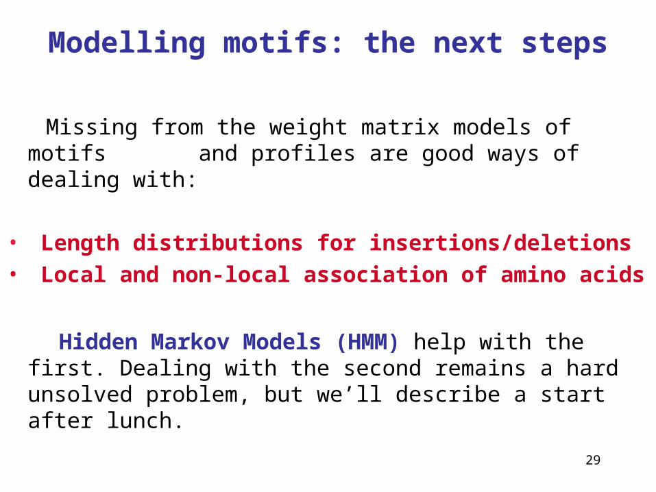
Modelling motifs: the next steps

Missing from the weight matrix models of motifs and profiles are good ways of dealing with:

• Length distributions for insertions/deletions• Local and non-local association of amino acids

Hidden Markov Models (HMM) help with the first. Dealing with the second remains a hard unsolved problem, but we’ll describe a start after lunch.

30

Hidden Markov Models

Processes {(St, Ot), t=1,…}, where St is the hidden

state and Ot the observation at time t, such that

pr(St | St-1, Ot-1,St-2 , Ot-2 …) = pr(St | St-1)

pr(Ot | St ,St-1, Ot-1,St-2 , Ot-2 …) = pr(Ot | St, St-1)

The basics of HMM were laid bare in a series of beautiful papers by L E Baum and colleagues around 1970, and their formulation has been used almost unchanged to this day.

31

A simple HMM (Churchill, 1989)

. . . . . .

. . . . . .A T C A A G G C G A T

A 0.4C 0.1G 0.1T 0.4

A 0.05C 0.4G 0.5T 0.05

O.O1O.9

O.1

O.99

hidden states

observations

32

Hidden Markov Models:extensions

Many variants are now used. For example, the distribution of O may depend only on previous S, or also on previous O values,

pr(Ot | St , St-1 , Ot-1 ,.. ) = pr(Ot | St ), or

pr(Ot | St , St-1 , Ot-1 ,.. ) = pr(Ot | St , St-1 ,Ot-1) .

Most importantly for us, the times of S and O may be

decoupled, permitting the Observation corresponding to State time t to be a string whose length and composition depends on St (and possibly St-1 and part or all of the previous Observations). This is called a hidden semi-Markov or generalized hidden Markov model, see later.

Some current applications of HMM to biology mapping chromosomes

aligning biological sequences

predicting sequence structure

inferring evolutionary relationships

finding genes in DNA sequence

Some early applications of HMM finance, but we never saw them

speech recognition

modelling ion channels

In the mid-late 1980s HMMs entered genetics and molecular biology, and they are now firmly entrenched.

34

The algorithms

As the name suggests, with an HMM the series O = (O1,O2 ,O3 ,……., OT) is observed, while the states S = (S1 ,S2 ,S3 ,……., ST) are not.

There are elegant algorithms for calculating pr(O|), arg max pr(O|) in certain special cases, and arg maxS pr(S|O,).

Here are the parameters of the model, e.g. transition and observation probabilities.

35

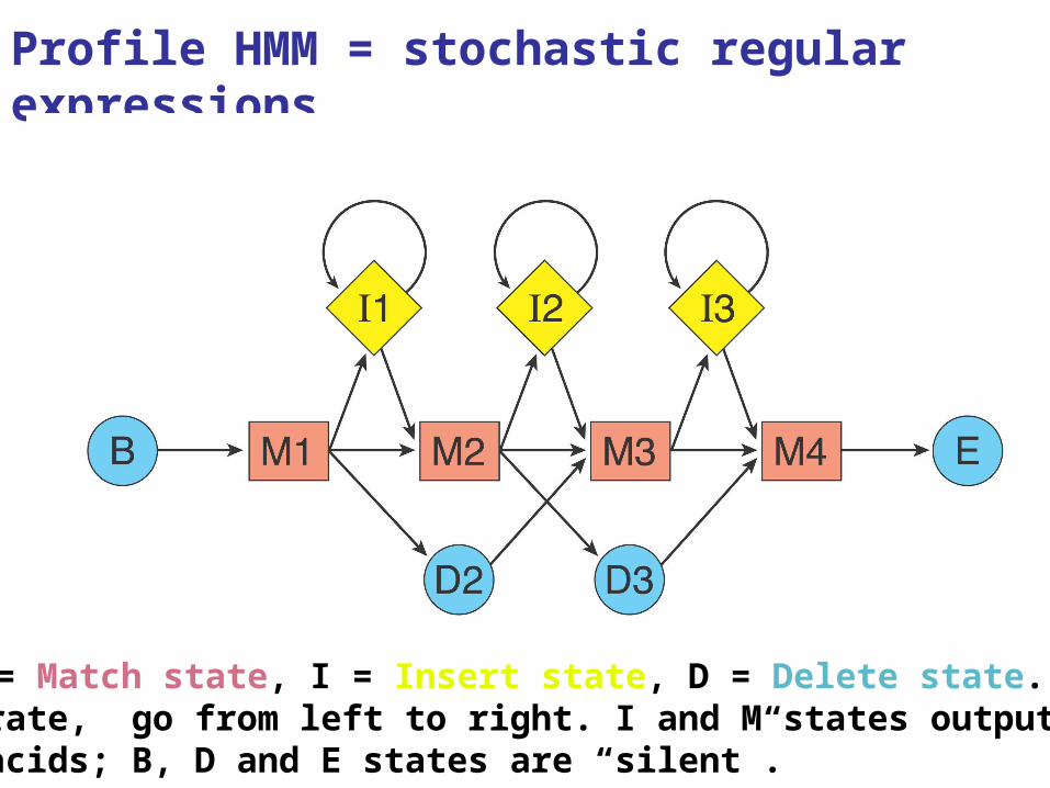
Profile HMM = stochastic regular expressions

M = Match state, I = Insert state, D = Delete state. To operate, go from left to right. I and M states output amino acids; B, D and E states are “silent”.

36

How profile HMM are used

Instances of the motif are identified by calculating log{pr(sequence | M)/pr(sequence | B)}, where M and B are the motif and background HMM.Alignments of instances of the motif to the HMM are

found by calculating

arg maxstates pr(states | instance, M).Estimation of HMM parameters is by calculating

arg maxparameterspr(sequences | M, parameters).

In all cases, we use the efficient HMM algorithms.

37

Pfam domain-HMM

Pfam is a library of models of recurrent protein domains. They are constructed semi-automatically using profile hidden Markov models.

Pfam families have permanent accession numbers and contain functional annotation and cross-references to other databases, while Pfam-B families are re-generated at each release and are unannotated.

See http://pfam.wustl.edu/

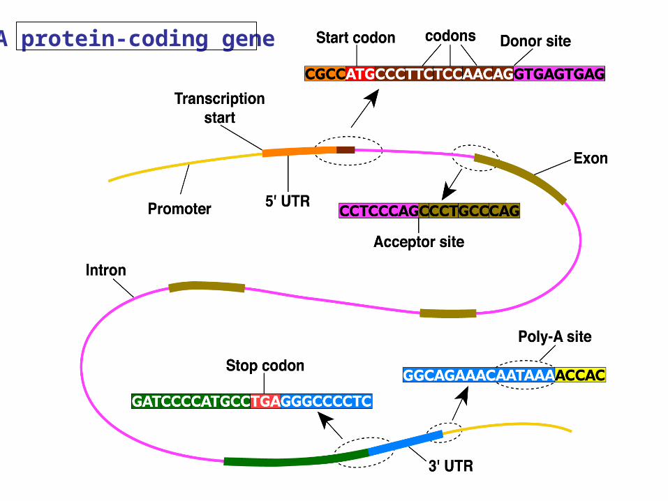
38

A protein-coding gene

39

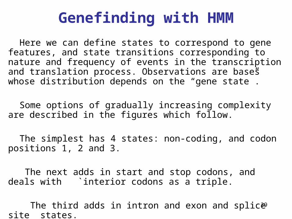
Genefinding with HMM

Here we can define states to correspond to gene features, and state transitions corresponding to nature and frequency of events in the transcription and translation process. Observations are bases whose distribution depends on the “gene state”.

Some options of gradually increasing complexity are described in the figures which follow.

The simplest has 4 states: non-coding, and codon positions 1, 2 and 3.

The next adds in start and stop codons, and deals with `interior codons as a triple.

The third adds in intron and exon and splice site states.

40

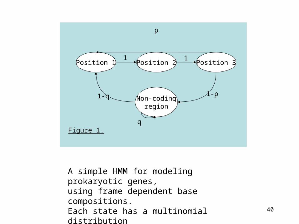
Position 1 Position 2 Position 3

Non-codingregion

p

1-q 1-p

q

1 1

Figure 1.

A simple HMM for modeling prokaryotic genes, using frame dependent base compositions.Each state has a multinomial distribution over {A, C, G, T} associated with it.

41

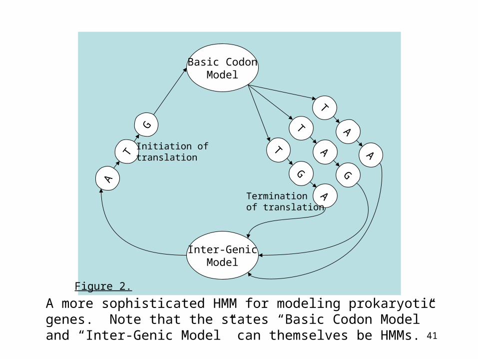
TT

G

AG

A

T

T

A

A

A

G

Basic CodonModel

Inter-GenicModel

Initiation oftranslation

Termination of translation

Figure 2.

A more sophisticated HMM for modeling prokaryoticgenes. Note that the states “Basic Codon Model” and “Inter-Genic Model” can themselves be HMMs.

42

Start Codon

Upstream Downstream

Stop CodonExon

3’ Splice Site 5’ Splice Site

Intron

Figure 3.

An simple hypothetical HMM for modeling eukaryotic genes, allowing for exon/intron structure. Each ofthe states can be an HMM or some other statistical model.

43

Generalized HMM

A drawback with ordinary HMM for genefinding is the tight coupling of state with observation. This leads to geometricduration distributions in each state, and this is not very close to what is observed in many cases.

Accordingly, Haussler and colleagues, and later Burge & Karlin moved to Generalized HMMs (GHMM), also called Hidden Semi-Markov Models, in which the state and the observation are decoupled : as we move from state to state, we output a DNA string of variable length, not just one base per one state transition. The length distribution can then be matched to the observed duration distribution in that state.

Increased computational complexity is the price we must pay.

44

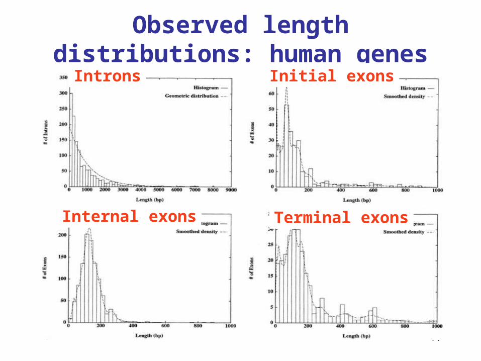
Observed length distributions: human genes

Introns Initial exons

Internal exons Terminal exons

45

Other approaches

There are a host of other approaches to genefinding which I am passing over in my effort to get quickly to the best current genefinders. Some of these are discussed in a disorganized way in Mount’s book, which is part of the reason that chapter is a mess.

Historically important was Grail, a genefinder based on neural networks, and a variety of ones using some form of discriminant analysis. All non-HMM approaches met the problem of weighting and combining the different pieces of information into an overall gene propensity score. This is dealt with naturally and elegantly by the Viterbi phase of HMM.

46

The idea behind a GHMM genefinder

States represent standard gene features: intergenic region, exon, intron, perhaps more (promotor, 5’UTR, 3’UTR, Poly-A,..).

Observations embody state-dependent base composition, dependence, and signal features.

In a GHMM, duration must be included as well. Finally, reading frames and both strands must

be dealt with.

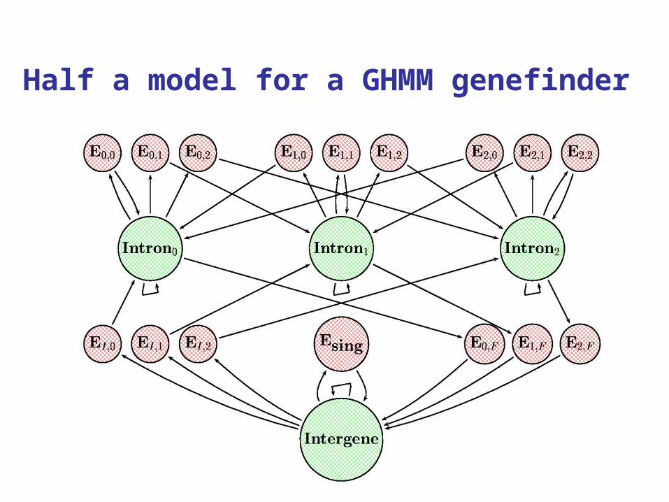
47

Half a model for a GHMM genefinder

48

Splice sites can be included in the exons

49

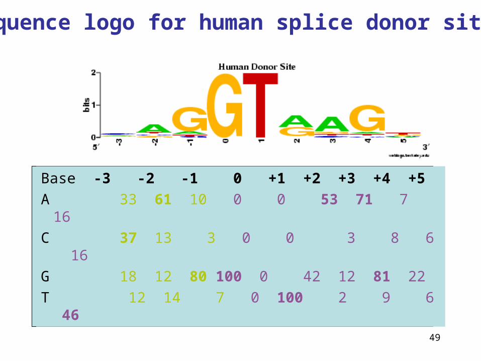
Base -3 -2 -1 0 +1 +2 +3 +4 +5

A 33 61 10 0 0 53 71 7 16

C 37 13 3 0 0 3 8 6 16

G 18 12 80 100 0 42 12 81 22

T 12 14 7 0 100 2 9 6 46

Sequence logo for human splice donor sites

50

Beyond position-specific distributions

The bases in splice sites exhibit dependence, and not simply of the nearest neighbor kind.

High-order (non-stationary) Markov models would be one option, but the number of parameters in relation to the amount of data rules them out.

The class of variable length Markov models (VLMMs) deriving from early research by Rissanen prove to be valuable in this context, see after lunch.

51

How gene GHMMs work: in brief

Instances of genes are identified by calculating log{pr(sequence | M)/pr(sequence | B)}, where M and B are the model and background HMMs. Alignments of instances to the gene HMM are found

by calculating

arg maxstates pr(states | instance, M). This gives the “best” gene annotation. Suboptimal

ones are also of interest. Estimation of HMM parameters is by calculating

arg max parameters pr(sequences | M, parameters). In all cases, we use the efficient HMM algorithms.

52

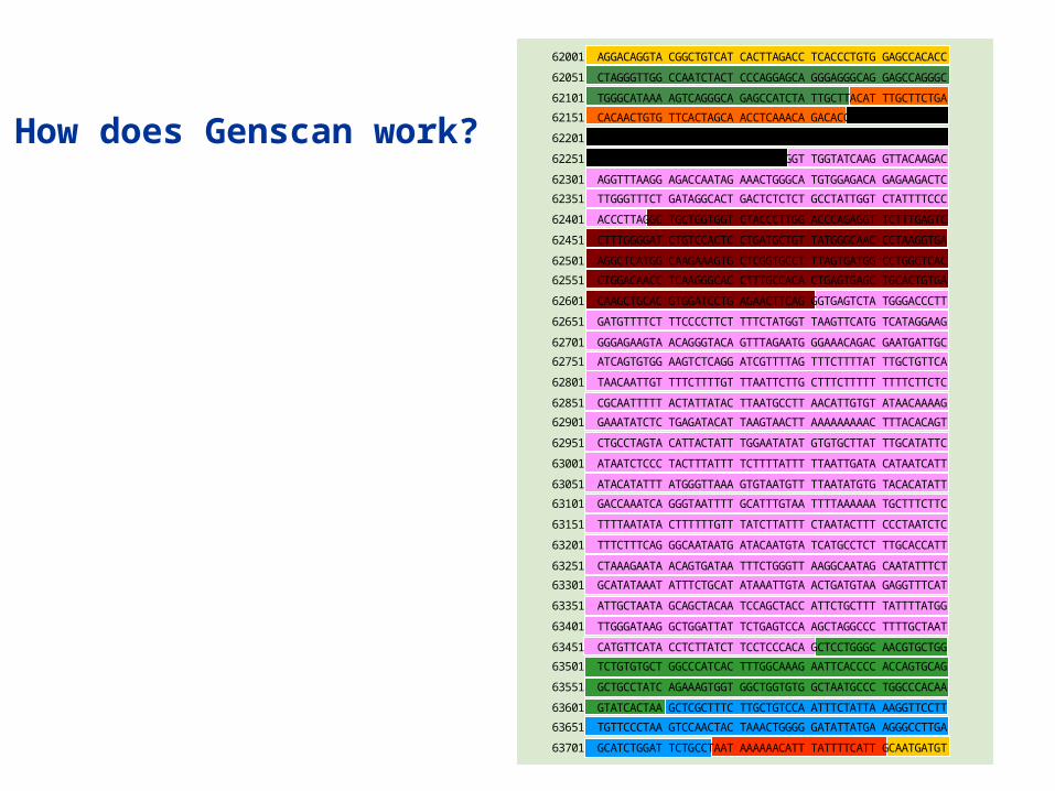
62001 AGGACAGGTA CGGCTGTCAT CACTTAGACC TCACCCTGTG GAGCCACACC

62051 CTAGGGTTGG CCAATCTACT CCCAGGAGCA GGGAGGGCAG GAGCCAGGGC

62101 TGGGCATAAA AGTCAGGGCA GAGCCATCTA TTGCTTACAT TTGCTTCTGA

62151 CACAACTGTG TTCACTAGCA ACCTCAAACA GACACCATGG TGCACCTGAC

62201 TCCTGAGGAG AAGTCTGCCG TTACTGCCCT GTGGGGCAAG GTGAACGTGG

62251 ATGAAGTTGG TGGTGAGGCC CTGGGCAGGT TGGTATCAAG GTTACAAGAC

62301 AGGTTTAAGG AGACCAATAG AAACTGGGCA TGTGGAGACA GAGAAGACTC

62351 TTGGGTTTCT GATAGGCACT GACTCTCTCT GCCTATTGGT CTATTTTCCC

62401 ACCCTTAGGC TGCTGGTGGT CTACCCTTGG ACCCAGAGGT TCTTTGAGTC

62451 CTTTGGGGAT CTGTCCACTC CTGATGCTGT TATGGGCAAC CCTAAGGTGA

62501 AGGCTCATGG CAAGAAAGTG CTCGGTGCCT TTAGTGATGG CCTGGCTCAC

62551 CTGGACAACC TCAAGGGCAC CTTTGCCACA CTGAGTGAGC TGCACTGTGA

62601 CAAGCTGCAC GTGGATCCTG AGAACTTCAG GGTGAGTCTA TGGGACCCTT

62651 GATGTTTTCT TTCCCCTTCT TTTCTATGGT TAAGTTCATG TCATAGGAAG

62701 GGGAGAAGTA ACAGGGTACA GTTTAGAATG GGAAACAGAC GAATGATTGC

62751 ATCAGTGTGG AAGTCTCAGG ATCGTTTTAG TTTCTTTTAT TTGCTGTTCA

62801 TAACAATTGT TTTCTTTTGT TTAATTCTTG CTTTCTTTTT TTTTCTTCTC

62851 CGCAATTTTT ACTATTATAC TTAATGCCTT AACATTGTGT ATAACAAAAG

62901 GAAATATCTC TGAGATACAT TAAGTAACTT AAAAAAAAAC TTTACACAGT

62951 CTGCCTAGTA CATTACTATT TGGAATATAT GTGTGCTTAT TTGCATATTC

63001 ATAATCTCCC TACTTTATTT TCTTTTATTT TTAATTGATA CATAATCATT

63051 ATACATATTT ATGGGTTAAA GTGTAATGTT TTAATATGTG TACACATATT

63101 GACCAAATCA GGGTAATTTT GCATTTGTAA TTTTAAAAAA TGCTTTCTTC

63151 TTTTAATATA CTTTTTTGTT TATCTTATTT CTAATACTTT CCCTAATCTC

63201 TTTCTTTCAG GGCAATAATG ATACAATGTA TCATGCCTCT TTGCACCATT

63251 CTAAAGAATA ACAGTGATAA TTTCTGGGTT AAGGCAATAG CAATATTTCT

63301 GCATATAAAT ATTTCTGCAT ATAAATTGTA ACTGATGTAA GAGGTTTCAT

63351 ATTGCTAATA GCAGCTACAA TCCAGCTACC ATTCTGCTTT TATTTTATGG

63401 TTGGGATAAG GCTGGATTAT TCTGAGTCCA AGCTAGGCCC TTTTGCTAAT

63451 CATGTTCATA CCTCTTATCT TCCTCCCACA GCTCCTGGGC AACGTGCTGG

63501 TCTGTGTGCT GGCCCATCAC TTTGGCAAAG AATTCACCCC ACCAGTGCAG

63551 GCTGCCTATC AGAAAGTGGT GGCTGGTGTG GCTAATGCCC TGGCCCACAA

63601 GTATCACTAA GCTCGCTTTC TTGCTGTCCA ATTTCTATTA AAGGTTCCTT

63651 TGTTCCCTAA GTCCAACTAC TAAACTGGGG GATATTATGA AGGGCCTTGA

63701 GCATCTGGAT TCTGCCTAAT AAAAAACATT TATTTTCATT GCAATGATGT

How does Genscan work?

53

Acknowledgements

Xiaoyue Zhao, UCB

Mauro Delorenzi (ISREC)

Sourav Chatterji, UCB

The SLAM team:

Simon Cawley, Affymetrix

Lior Pachter, UCB

Marina Alexandersson, FCC

54

ReferencesBiological Sequence AnalysisR Durbin, S Eddy, A Krogh and G MitchisonCambridge University Press, 1998.

Bioinformatics The machine learning approach

P Baldi and S BrunakThe MIT Press, 1998

Post-Genome InformaticsM KanehisaOxford University Press, 2000